ME 513 VEHICLE DYNAMICS

Term Project:

ROAD VEHICLE RIDE SIMULATION AND

ANIMATION

Gönenç Gürsoy

Eren Kahraman

Anna Prach

Larasmoyo Nugroho

Middle East Technical University

Ankara, Turkey

June 2012

2

List of Symbols

� - sprung mass

��,�� -unsprung masses

�� - moment of inertia about roll axis

� - moment of inertia about pitch axis

- effective vertical stiffness of a suspension

� - effective damping constant of adamper

� - tire spring coefficient

Subscripts:

� – front left

� – front right

�� – rear left

�� – rear right

3

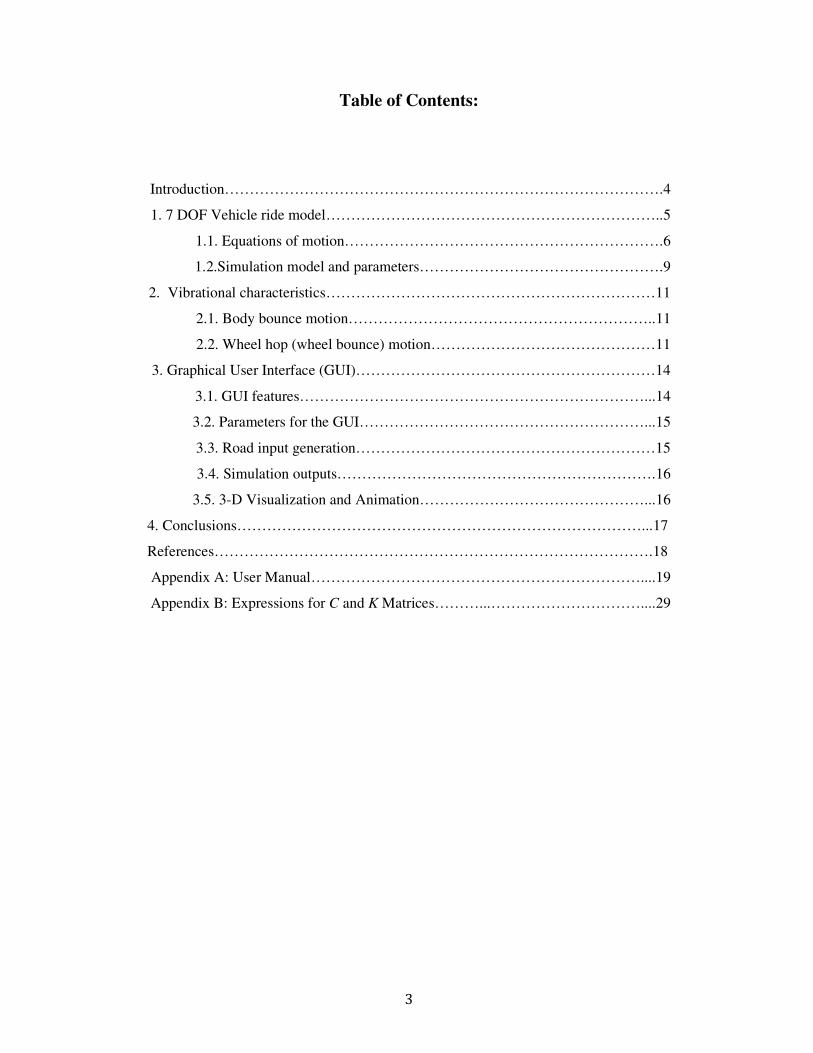
Table of Contents:

Introduction…………………………………………………………………………….4

1. 7 DOF Vehicle ride model…………………………………………………………..5

1.1. Equations of motion……………………………………………………….6

1.2.Simulation model and parameters………………………………………….9

2. Vibrational characteristics…………………………………………………………11

2.1. Body bounce motion……………………………………………………..11

2.2. Wheel hop (wheel bounce) motion………………………………………11

3. Graphical User Interface (GUI)……………………………………………………14

3.1. GUI features……………………………………………………………...14

3.2. Parameters for the GUI…………………………………………………...15

3.3. Road input generation……………………………………………………15

3.4. Simulation outputs……………………………………………………….16

3.5. 3-D Visualization and Animation………………………………………...16

4. Conclusions………………………………………………………………………...17

References…………………………………………………………………………….18

Appendix A: User Manual…………………………………………………………....19

Appendix B: Expressions for C and K Matrices………...…………………………....29

4

Introduction

This project focuses on development of the MATLAB based Graphical User

Interface (GUI) for a road vehicle ride simulation and animation.

A road vehicle simulation model is one of the important elements to be

developed while designing the GUI. The most simple road vehicle model is

represented by two degrees of freedom quarter car model [Ref. 1]. Half-car models

are developed with four degrees of freedom and, in general, represent vehicle

longitudinal dynamics and vertical dynamics of front and rear wheels, or can be used

to analyze lateral dynamics of a vehicle together with the vertical motion of right and

left wheels [Ref. 2]. Three-dimensional full-vehicle models have at least six degrees of

freedom, which may increase up to hundreds [Ref.3]. The complexity of the vehicle

model depends of the number of components included in the model, fidelity,

assumptions used.

While studying the vehicle ride, another important issue is the excitation

sources, which are the inputs to the simulation model. There are multiple sources of

vehicle ride vibrations excitations, and the most general are classified as road

irregularities and on-board sources. Effect of road roughness on the vehicle motion is

of the scope of this project. Road roughness is described by the elevation profile along

the wheel tracks over which the vehicle passes [Ref. 4]. The GUI developed such that

a user will model the road inputs, enabling to specify the road roughness and bumps

on the road surface.

5

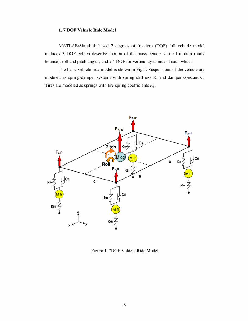
1. 7 DOF Vehicle Ride Model

MATLAB/Simulink based 7 degrees of freedom (DOF) full vehicle model

includes 3 DOF, which describe motion of the mass center: vertical motion (body

bounce), roll and pitch angles, and a 4 DOF for vertical dynamics of each wheel.

The basic vehicle ride model is shown in Fig.1. Suspensions of the vehicle are

modeled as spring-damper systems with spring stiffness K, and damper constant C.

Tires are modeled as springs with tire spring coefficients �.

Figure 1. 7DOF Vehicle Ride Model

Pitch

a

b

c

6

1.1. Equations of Motion

The dynamic vehicle ride model is developed using Newton’s Second Law.

Equations of motion that describe a vehicle 7 DOF ride model are the following.

Force equation along z-axis:

for sprung mass:

��� = ��,�� + ��,�� + ��,�� + ��,��

for unsprung masses:

������� = ��_�,�� ������� = ��_�,��

������� = ��_�,�� ������� = ��_�,��

Moment equations about x and y axis:

���� = ���,�� − ���,�� + ���,�� − ���,��

��� = −���,�� − ���,�� + ��,�� + ��,��

Assuming small pitch and roll angles, and using assumptions !"#� ≈ � ,

!"#� ≈ � expressions for the vertical forces acting on sprung mass can be written as:

��,�� = %−� − �� − �� + ���&�� + %−�' − ��' − ��' + �'��&��� ��,�� = %−� − �� + �� + ���&�� + %−�' − ��' + ��' + �'��&���

��,�� = (−� + � − �� + ���)�� + %−�' + �' − ��' + �'��&��� ��,�� = (−� + � + �� + ���)�� + %−�' + �' + ��' + �'��&���

Forces, acting on unsprung masses are given by following expressions:

��_�,�� = (� + �� + ��)�� + %�' + ��' + ��' − �'��&��� − ���%�� + ���& + *����� ��_�,�� = (� + �� − ��)�� + %�' + ��' − ��' − �'��&��� − ���%�� + ���& + *�����

��_�,�� = (� − � + ��)�� + %�' − �' + ��' − �'��&��� − ���(�� + ���) + *����� ��_�,�� = (� − � − ��)�� + %�' − �' − ��' − �'��&��� − ���(�� + ���) + *�����

7

Where *�� , *�� , *�� , *�� are the road displacement inputs acting on the

corresponding wheels, ��� , ��� , ��� , ��� - tire spring coefficients of the

corresponding wheels, and

��� , ��� , ��� , ��� - wheels vertical displacements (vertical displacements of

unsprung masses).

In the matrix form equations of motion describing the 7 DOF vehicle ride

model can be written as:

+M-.� = +C-.' + +K-. + +F-*

where state vector is defined as follows:

. = 2�, �, �, ���, ���, ��� , ���34

and the input vector is gives as:

* = 2*��, *��, *�� , *��34.

Expressions for matrices in the state space equation above are:

+M- =56666667�0000000�� 0000000�0000000���0000000���0000000��� 0000000���9:

:::::;

� = 2���3<×<

where

�>> = −��� − ��� − ��� − ���

�>? = −�%��� + ���& + �%��� + ���&

�>@ = −�%��� + ���& + (��� + ���) �>A = ��� �>B = ���

�>C = ��� �>< = ���

�?> = −�%��� + ���& + �%��� + ���&

�?? = −�?%��� + ��� + ��� + ���&

�?@ = ��%��� − ���& + � (��� − ���)

�?A = ���� �?B = −����

�?C = ���� �?< = −����

�@> = −�%��� + ���& + (��� + ���) �@? = ��%��� − ���& + � (��� − ���) �@@ = −�?%��� + ���& − ?(��� + ���) �@A = ���� �@B = ����

�@C = − ���

8

�@< = − ���

�A> = ��� �A? = ���� �A@ = ���� �AA = −��� �AB = �AC = �A< = 0

�B> = ���

�B? = −����

�B@ = ����

�BB = −���

�BA = �BC = �B< = 0

�C> = ��� �C? = ���� �C@ = − ��� �CC = −��� �CA = �CB = �C< = 0

�<> = ���

�<? = −����

�<@ = − ���

�<< = −���

�<A = �<B = �<C = 0

+- = +-<×<

where

>> = −�� − �� − �� − ��

>? = −�%�� + ��& + �%�� + ��&

>@ = −�%�� + ��& + (�� + ��) >A = �� >B = ��

>C = �� >< = ��

?> = −�%�� + ��& + �%�� + ��&

?? = −�?%�� + �� +�� +��&

?@ = ��%�� − ��& + � (�� − ��) ?A = ��� ?B = −���

?C = ��� ?< = −���

@> = −�%�� + ��& + (�� + ��) @? = ��%�� − ��& + � (�� − ��) @@ = −�?%�� + ��& − ?(�� + ��) @A = ���

@B = ���

@C = − �� @< = − ��

A> = �� A? = ��� A@ = ��� AA = −(�� + ���) AB = AC = A< = 0

B> = ��

B? = −���

B@ = ���

BB = −(�� + ���) BA = BC = B< = 0

C> = �� C? = ��� C@ = − �� CC = −(�� + ���) CA = CB = C< = 0

<> = ��

9

<? = −���

<@ = − ��

<< = −(�� + ���) <A = <B = <C = 0

+F- =5666667 000000000000���0000���0000���0000���9:

::::;

1.2.Simulation Model and Parameters

The 7 DOF vehicle ride model was developed in MATLAB/Simulink, and its

Simulink block diagram is illustrated in the Fig.2.

Figure 2. MATLAB/Simulink Block Diagram of 7 DOF Model

Vehicle and suspension parameters used for the model were obtained from Ref.

5, and are given in the Tables 1- 3.

Angle convension:

positive pitch is nose up

positive roll is rolling right

positive height is upwards

7DOF Model:Body bounce, roll angle, pitch angle, wheel hop

Road inputs

7

z_rr

6

z_rl

5

z_fr

4

z_fl

3

theta

2

phi

1

BodyBounce

-K-

-K-

b

a

c_fl

c_fr

c_rl

c_rr

k_fl

m

k_tfl

k_tfr

k_trl

k_trr

k_fr

0

0

0

0

Iy

Ix

M

c

k_rl

k_rr

ki

kt

ci

geom

mass

input_v ec

input_dot_v ec

q_v ec

output_v ecfcn

Ride_Model

1

s

Integrator1

1

s

Integrator

4

qFL

3

qFR

2

qRL

1

qRR

10

Table 1.

Mass, Inertia and Geometry Parameters Value

Vehicle body mass sprung mass (M) 1355 kg

Vehicle body inertia about x-axis (Ix) 1920 kg⋅m^2

about y-axis (Iy) 1000 kg⋅m^2

Distance from vehicle C.G to front wheels (a) 1.179 m

rear wheels (b) 1.541 m

Wheel track/2 front (c) 0.7 m

rear (c) 0.7 m

Table 2.

Suspension Parameters Value

Suspension Stiffness

front right (k_fr) 45000 N/m

front left (k_fl) 45000 N/m

rear right (k_rr) 34615 N/m

rear left (k_rl) 34615 N/m

Suspension Damping

front right (c_fr) 4500 N·s/m

front left (c_fl) 4500 N·s/m

rear right (c_rr) 4500 N·s/m

rear left (c_rl) 4500 N·s/m

Table 3.

Wheel Parameters Value

Wheel mass unsprung mass (m) 40 kg

Wheel radius (tire_radius) 0.3 m

Tire spring constant

front right (k_tfr) 200000N/m

front left (k_tfl) 200000N/m

rear right (k_trr) 200000N/m

rear left (k_trl) 200000N/m

11

2. Vibrational Characteristics

Vibrational characteristics of a road vehicle include characteristics of vehicle

vibrations at frequencies from 40 to 400 Hz, which are caused by road irregularities,

and vibrations at frequency range of 1000 - 2000 Hz, caused by machinery whines,

gears, etc.

Effect of road roughness on the vehicle ride is analyzed in this project.

2.1. BodyBounce Motion

Body bounce is the vertical motion of the sprung mass on the suspension

spring. Approximate value of the body bounce frequency can be calculated using the

following formula:

DEE = FGH�

whereGH is the total suspension stiffness, which is equal to the sum of stiffness

coefficients of individual suspensions.

For the given vehicle and suspension parameters, the value of the body bounce

frequency is obtained to be equal to DEE = 1.72M�.

2.2. Wheel Hop (Wheel Bounce) Motion

All individually sprung wheels have a vertical motion (wheel hop) mode,

which is excited by the road inputs. Wheel hop frequencies are much higher than the

body bounce frequencies, so the sprung mass tends to stay stationary during wheel

hop. Approximate value of the wheel hop frequency can be calculated using a quarter

car model:

DNO = FGH + G��

For the given vehicle, suspension stiffness is different for the front and rear

suspensions, therefore, wheel hop frequencies for front and rear wheels are calculated

separately, and are equal to: DNO_��PQ� = 12.46M�, DNO_�TU� = 12.19M�.

12

To show the frequency separation of the body bounce and wheel hop modes,

simulation is performed for the case when vehicle wheels are being excited with the

sinusoidal signal with frequency equal to the wheel hop frequency. The input signal

and vehicle responses in terms of the body bounce and wheel hop motions are

illustrated in Fig.3-6 below. The input magnitude is 0.05m, and input frequency is

equal to the approximate value of the wheel hop frequency.

Figure 3. Road Input

Figure 4. Body Bounce Motion

0 1 2 3 4 5 6 7 8 9 10-0.06

-0.04

-0.02

0

0.02

0.04

0.06

Time, s

Magnitude, m

13

Figure 5. Wheel Hop Motion of Front Wheels

Figure 6. Wheel Hop Motion of Rear Wheels

14

3. Graphical User Interface (GUI)

Graphical User Interface (GUI) for the full vehicle ride model was developed in

MATLAB and is targeted for use on Windows platform. The main interface window is

shown in Fig. 7.

Figure 7. Graphical User Interface for Vehicle Ride Model

3.1. GUI Features

GUI for the full vehicle ride model enables:

• Enter/load/save vehicle parameters;

• Enter vehicle average velocity;

• Enter travel distance;

15

• Specify road input in terms of road roughness and bumps;

• Simulate the 7 DOF full vehicle ride model;

• Plot the variables of interest, zoom and save plots;

• 3-D animation of the ground vehicle motion;

In addition to input data save/load options, Project Load and Project Save

option is available in GUI, which allows user to save the vehicle parameters, road

configuration and simulation responses to a new folder, and loaded again when

needed.

3.2. Parameters for the GUI

GUI uses a 7 DOF vehicle ride model, and therefore, a set of parameters is

needed to be entered/loaded before starting the simulation. These parameters include

mass, inertia and geometric characteristics, suspension parameters and wheels/tires

characteristics. Tables 1- 3 include the list of the parameters required. Default set of

parameters is taken from the Ref. [5]. GUI allows user to enter parameters, save them,

and load the existing data.

3.3. Road Input Generation

Road input generation algorithm enables to specify the road inputs used in the

vehicle ride model simulation. The road input (road surface profile) can be selected as:

• Flat road;

• Sinusoidal input is specified by its magnitude and the wave number (# ).

Excitation frequency is computed taking into account the vehicle speed (V):

= W# [Hz]; the value of excitation frequency is displayed in GUI. The

excitation frequency is the frequency of the sine wave road input to the vehicle;

• Random signal, given by its standard deviation;

• Bumps on the road surface can be set by specifying location with respect to the

travel distance and height for each bump. Bumps can be generated as

symmetric (for both wheels) and asymmetric (for left or right wheel only).

16

Once the road surface profile configuration is being generated, GUI allows user to

save the road configuration, and load it when desired.

3.4. Simulation Outputs

After running the simulation, plots of the following variables are displayed in

the GUI window:

• Body bounce;

• Vertical acceleration;

• Pitch angle;

• Roll angle;

• Vertical displacement for each wheel.

Each plot can be zoomed, edited and saved as a figure file.

3.5. 3-D Animation

The animation of ground vehicle dynamic model in the virtual reality

environment is performed by the Simulink 3D Animation. After starting the

simulation, a virtual world opens in the Simulink 3D Animation viewer by default. A

simulation starts running, and the virtual world is animated using signal data from the

simulation model. The following data are required as an input to the animation block

set: body bounce motion, pitch and roll angles, wheels displacements. User can set

positions and properties of VRML object (camera location, zoom in/out). The snapshot

of the vehicle’s animated motion is shown in Fig.8.

17

Figure 8. 3-D Visualization of the Vehicle Motion

4. Conclusions

A MATLAB based Graphical User Interface is developed for the full vehicle

ride model. The GUI allows simulation of the 7 DOF full vehicle ride model for

specified road inputs, visualization of the vehicle motion, and plots of the output

variables, which include body bounce, pitch and roll angles, and wheels vertical

motion. User is allowed to enter, load and save vehicle parameters, and also select the

desired road inputs by specifying road surface profile (flat road, sinusoidal or random

signal), and bumps in the desired locations on the road surface. GUI allows saving and

loading the generated road input. 3-D animation of the road vehicle motion is provided

by the Simulink 3-D Animation.

Appendix A includes the User Manual for the full vehicle ride simulation and

animation GUI.

18

References

1. Thompson, A.G. The effect of tire damping on the performance of vibration

absorbers in an active suspension. Journal of Sound and Vibration, 1989, 133(3), 457-

465.

2. Campos, J., Davis, L., Lewis, F.L., Ikenaga, S., Scully, S. and Evans, M. Active

SuspensionControl of Ground Vehicle Heave and Pitch Motions. Proceedings of the

7th Mediterranean Conference on Control and Automation (MED99)Haifa, Israel,

1999).

3. Stone, M.R. and Demetriou, M.A. Modeling and Simulation of Vehicle Ride and

Handling Performance. Proceedings of the 15th IEEE International Symposium on

Intelligent Control (ISIC2000)Rio, Patras, Greece, 2000).

4. T. D. Gillespie, Fundamentals of Vehicle Dynamics,Warrendale, PA : Society of

Automotive Engineers, c1992. 01/01/1992 xxii, 495 p.

5. S. Roy and Z. Liu, "Road Vehicle Suspension and Performance Evaluation using a

Two Dimensional Vehicle Model", Int. J. of Vehicle Systems Modeling and Testing,

3(1/2), 68-93, 2008.

6. http://www.mathworks.com/

19

APPENDIX A

User Manual

In this section, “how GUI can be used” is explained step by step by illustrating simple

simulation examples.

Since the GUI is developed using MATLAB, make sure that MATLAB is installed in

the computer. Also, the folder which includes all project files should be chosen as the

“working directory” in MATLAB. In Figure A.1, a picture of Matlab environment is

shown. Here, the folder, GUI_05302012, which includes all project files are chosen as

working directory. Once the working directory is chosen properly, we can start.

Figure A.1

20

Opening the GUI Window:

To open the GUI, the M-file “RideModelSimilator.m” needs to be run. The following

GUI window will appear on the screen.

Figure A.2

Loading Vehicle Parameters:

On the left upper part of the GUI, Figure A.2, vehicle parameters can be seen.

Parameters should be loaded using the “Load Vehicle Parameters” button. When it is

pressed the following window is shown on the screen.

Figure A.3

21

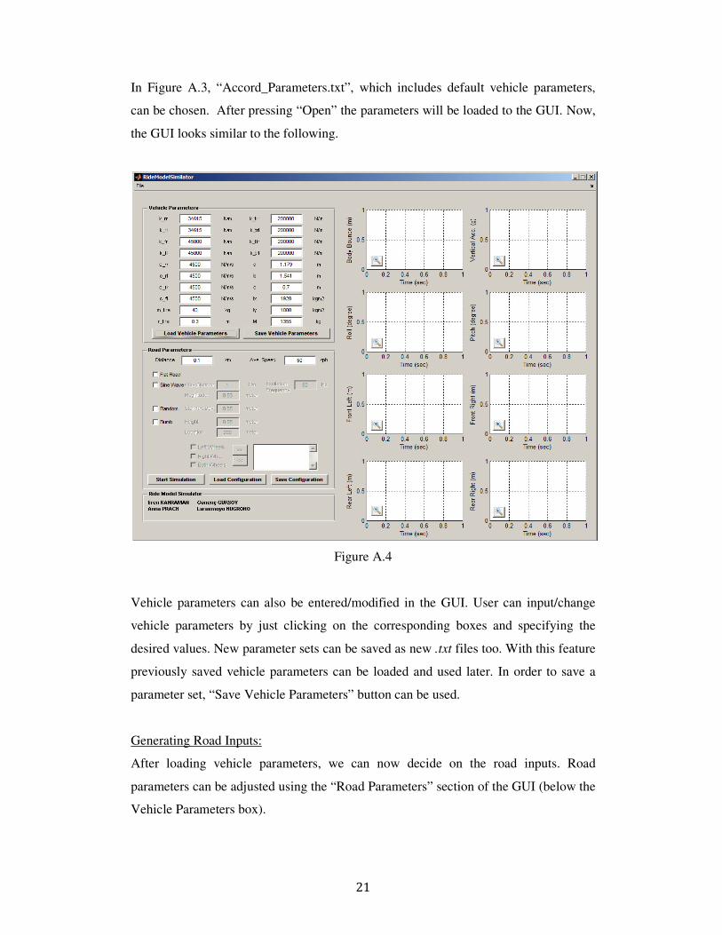
In Figure A.3, “Accord_Parameters.txt”, which includes default vehicle parameters,

can be chosen. After pressing “Open” the parameters will be loaded to the GUI. Now,

the GUI looks similar to the following.

Figure A.4

Vehicle parameters can also be entered/modified in the GUI. User can input/change

vehicle parameters by just clicking on the corresponding boxes and specifying the

desired values. New parameter sets can be saved as new .txt files too. With this feature

previously saved vehicle parameters can be loaded and used later. In order to save a

parameter set, “Save Vehicle Parameters” button can be used.

Generating Road Inputs:

After loading vehicle parameters, we can now decide on the road inputs. Road

parameters can be adjusted using the “Road Parameters” section of the GUI (below the

Vehicle Parameters box).

22

In that section, the distance to be travelled and the average speed of travel should be

entered by the user. Let’s enter these inputs as 0.4 km and 30 kph into the boxes called

“Distance” and “Ave. Speed”. Then choose the “Flat Road” as the road type. And

click on the “Start Simulation” button. A simulation window illustrated in Figure A.5

will appear on the screen.

Figure A.5

When the simulation ends simulation results can be viewed by the corresponding plots

in the right side of the GUI window (Figure A.6). In this example, since the road is

chosen as flat, no input is given to the vehicle during the simulation. Body bounce,

vertical acceleration, roll and pitch angles and deflections of wheels are shown in the

right side of the GUI. All simulation results are zero since no input is given.

23

Figure A.6

Now, let us illustrate how to run simulations for different road inputs.

Simulations Using Sine Wave Input:

Now click on the “Sine Wave” check box in order to give a sine wave input to the

vehicle. When the “Sine Wave” road profile is chosen, “Wave Number”, “Magnitude”

and “Excitation Frequency” boxes will be activated. Here user should enter the wave

number and the magnitude of the sine wave input into the “Wave Number” and

“Magnitude” boxes. After entering these inputs the corresponding excitation frequency

is calculated automatically and its value will appear in the “Excitation Frequency”

box.

Now let us enter wave number and magnitude of the oscillations as 1.5 and 0.03, then

the excitation frequency will automatically appear as 12.5 Hz. Note that this excitation

frequency is the wheel-hop frequency of that car model. GUI window is illustrated in

Figure A.7. Then pressing “Start Simulation” button, simulation will start and the

24

visualization window will appear. When the simulation ends GUI will appear as

shown in Figure A.8.

The Sine wave road input can be deactivated by a single click on a “Sine Wave” check

box.

Figure A.7

25

Figure A.8

Simulations Using Bumps and Random Inputs

Single click on the “Bump” box will activate a bump input option for the road profile

generation. Bumps can be specified by entering their heights and locations (location is

specified with respect to the travel distance) into the boxes “Height” and “Location”.

Let’s enter height as 0.05 (as default) and the location as 20 (which implies that a

bump is given as an input at the 20th

meter of the ride). Note that bump location cannot

be greater than the travel distance. Now, if we want to specify this bump as an input to

the left wheel, a single click on the check box “Left Wheels” followed by pressing the

right arrow button will add the specified bump to the box on the right (Figure A.9).

Now change the location as 50 and make it an input to the right wheels by clicking the

check box called “Right Wheels”, second by pressing the right arrow button to

generate it in the box. We may also use random inputs at the same time. Press

“Random” check box. Press “Start Simulation” button will run the simulation. GUI

window is shown in Figure A.10.

26

Figure A.9

Note that bumps as road input types can be given simultaneously for right and left

wheels. This option is activated by a single click on the “Both Wheels” check box.

A generated road profile can be saved using “Save Configuration” button and a pre-

saved configuration can be loaded using “Load Configuration” button located in the

“Road Parameters” section of the GUI.

27

Figure A.10

About Stopping The Simulations

If the simulation time becomes too long due to a large input of the travel distance or

travel velocity is very slow, the simulation can be stopped. In order to stop the

simulation the following steps should be performed: single click on the “Simulation”

button located in the visualization window, and then click on the “Stop” button will

stop the simulation.

Adjusting Different View Points

User can adjust the view points by using the up/down and left/right arrows on the

keyboard. This way angular view can be adjusted. By using up/down buttons while

holding the “SHIFT” button, it becomes possible to zoom in/out the vehicle. By using

up/down buttons while holding “ALT” button, camera gains altitude or descents. Also

by using left/right buttons while holding “ALT” button, camera is translated to the left

or right. A different views can be seen Figure A.11.

28

Figure A.11

APPENDIX B

C and K Matrices