BINARY-DIFFUSION COEFFICIENTS

FOR LIQUIDS

w; ABBAS • AUZADEH

BSc.Tech; MSc; DIG

Department of Chemical Engineering and Chemical Technology

IMPERIAL COLLEGE

University of London

December 1981

A thesis submitted for the degree of Doctor of Philosophy

of the University of London

T 0 :

The man who once told me

"We come and go with sufferings,

and in between, experience a few

real happy moments. ..

Nothing we have remains, but our

knowledge, ideas and thoughts.

Them, can never be lost or taken

away from us,

and them, what better than

to leave behind".

M.H. ALIZADEH ESQ. - ray father

A B S T R A C T

In view of the scarcity of reliable thermophysical property data, in

particular, of liquid-phase diffusion coefficients, this thesis describes

the design, construction and use of an apparatus which enables the measure-

ment of the binary diffusion coefficients of liquids with an accuracy of

±1%, A complete analysis of the theory of the instrument based upon the

phenomenon of Taylor dispersion is presented. An instrument has been

designed such that it operates very nearly in accordance with the simplest

mathematical description of the dispersion of a solute pulse in a fluid

in laminar flow within a long, straight circular cross-section tube. The

small departures of the instrument from its ideal model are evaluated as

corrections which include the effects of non-zero volumes of the injected

pulse and the concentration monitor, the coiling of the diffusion tube,

its non-uniformity and non-circularity of the cross-section and the varia-

tion of the fluid properties with composition. Owing to the instrument

design and under the selected experimental conditions, the effect of such

corrections are found to be either negligible or less than one percent.

Experimental results are persented which confirm that the instrument does

indeed operate in accordance with the theory of it.

Experimental data for the binary diffusion coefficients of three binary

liquid mixtures, n-hexane + n-heptane, n-hexane + n-octane and n-heptane +

n-octane, of various compositions in the temperature range 20°C to 70°C

and at a pressure of 1 bar are reported. The accuracy and precision of

these measurements are estimated to be ±1% and ±0.5% respectively. The

experimental data have been used to assess the validity of the theoretical

descriptions of diffusion in liquid mixtures, as well as testing several

estimation procedures, which are in current use.

ACKNOWLEDGEMENTS

The author is forever indebted and grateful to his supervisor.

Dr. W.A. Wakeham for his continuous encouragement, excellent counsel and

guidance during the course of this work.

The author wishes to express his sincere gratitude to his previous

supervisor Professor D.L. Trimm (U.N.S.W., Australia) who, together with

Dr. Hall and Mr. W. Watkins (ESSO Research Centre, Abingdon) have been a

great help in the early stages of the present work. The industrial

scholarship awarded to the author by ESSO Research Centre at Abingdon in

order to cover the equipment expenditure is gratefully appreciated.

Special thanks are due to the author's laboratory colleagues, Drs. J.

Menashe and V. Vesovic, and, in particular. Professor C.A. Nieto de Castro

(IST, Lisbon) whose friendship and continuous assistance and guidance

in fruitful discussions are deeply appreciated.

The author extends his thanks to Messrs. W.D. Geal, R. Wood and M.J. Dix

who have helped in the construction of the equipment; to Mr. S. Ranson,

the Technical Director of SPECAC for his assistance in modifying the

injection valve5 to Miss M. McNeile for her skillful typing of this

thesis; to Mr. I. Drummond of Analytical Services, and to Miss P. Browett

and Mrs. C. Fletcher, the two excellent and most helpful Departmental

Librarians.

Finally, the author wishes to express his deepest gratitude and appreciation

to his parents for their care and concern, trust and encouragement, as well

as their moral and financial support, not only during the course of this

work, but also throughout the author's education. Without them it would

have been impossible to carry out this work.

C O N T E N T S

Abstract

Acknowledgements

INTRODUCTION 1

CHAPTER 1 - Isothermal Diffusion and Diffusion Coefficients 5

1.1 - Basic Concepts and Definitions 5

1.1.1 - Isothermal Diffusion 5

1.1.2 - Diffusion Coefficient 6

1.1.3 - Unidirectional Diffusion 7

1.1. M- - Binary Systems 8

1.1.5 - Binary Diffusion Coefficient 9

1.1.6 - Binary-, Self-, and Tracer-Diffusion Coefficients 10

1.1.7 - Chemical Potential Driving Force 13

1.1.8 - The Phenomenological Equation of Diffusion in

Irreversible Thermodynamics 14-

1.2 - Models for Diffusion in Liquids 18

1.2.1 - The Hydrodynamic Model for Diffusion 19 1.2.2 - Kinetic Models of Diffusion 23

1.2.3 - The van der Waals' Model 28

1.3 - The Rigorous Theory of the Transport Properties of Dense Fluids 34

1.3.1 - Statistical Mechanical Theory 35

1.3.2 - The Rice-Allnat Theory 37

1.3.3 - Method of Time Correlation Functions 39

1.3.4 - The Technique of Molecular Dynamics Simulation 40

1.4 - Experimental Methods of Measuring Binary-Diffusion Coefficients For Liquids 46

1.4.1 - Free Diffusion Methods 47

1.4.2 - Steady-State Diffusion - The Diaphragm-Cell Technique 56

1.4.3 - Restricted Diffusion - The Conductance Method 59

1.4.4 - Taylor Dispersion Technique 60

1.4.5 - Other Important Methods 64

CHAPTER 2 - The Theory of the Experimental Method 66

2. - Introduction 66

2.1 - The Principle of the Experimental Method 66

2.2 - Practical Considerations 74

2.3 - Concentration Distribution Determination 75

2.3.1 - Temporal Moments 75

2.3.2 - Zeroth-Order Approximation 76

2.3.3 - First-Order Approximation 77

2.3.4 - The Concentration Monitor 79

2.3.5 - A Section of the Diffusion Tube 79

2.3.6 - A Small Volume at the Tube Exit 82

2.4 - Sample Introduction 86

2.5 - Diffusion Tube Geometry 87

2.5.1 - Helical Diffusion Tube 88

2.5.2 - The Connecting Tube 91

2.5.3 - Non-Uniform Diffusion Tube 94

2.5.4 - Non-Circular Cross-Section 101

2.6 - Concentration-Dependent Fluid Properties 102

2.6.1 - Concentration-Dependent Diffusion Coefficient 103

2.6.2 - Concentration-Dependent Density 105

2.7 - Summary of the Theoretical Analysis 107

CHAPTER 3 - Apparatus and Experimental Procedure 112

3. - Introduction 112

3.1 - Apparatus Design 112

3.2 - The Diffusion Tube 114

3.2.1 - Material of the Tube 114

3.2.2 - Design Study For Optimum Geometry of the Diffusion

Tube 124

3.2.3 - Summary of the Final Design Criteria and Constraints 127

3.2.4 - The Design Calculations 128

3.2.5 - The Results of the Design Calculations 129

3.2.6 - Conclusions of the Design Study 139

3.2.7 - The Apparatus Constants 139

3.3 - The Injection Valve 140

3.4- The Gravity Feed Reservoir 142

3.5 - The Temperature Measuring Device 142

3.6 - The Refractive Index Detector 144

3.7 - Working Equations 144

3.7.1 - Density of the Liquid Mixture 144

3.7.2 - The Reference Composition 145

3.7.3 - Ideal Moments of the Distribution and the Diffusion

Coefficients of Liquids 146

3.8 - Analysis of the Eluted Distributions 147

3.8.1 - Data Analysis: Problems and Their Solutions 148

3.8.2 - Algorithm for Data Analysis 151

3.9 - Experimental Procedure 152

3.1Q - Performance of the Equipment 156

3.10.1 - Departures From the Ideal Model 156

3.10.2 - Linearity of the Detector 159

3.10.3 - The Reference Composition 159

3.10.4 - Reproducibility of the Results and Precision 160

3.10.5 - Accuracy of the Results 161

CHAPTER 4 - Results 168

4. - Introduction 168

CHAPTER 5 - Discussion 195

5. - Introduction 195

5.1 - Data for the Properties of the Pure Components and Their Mixtures 195

5.2 - The Molecular Dynamics Approach to the Interpretation of

Binary Diffusion Coefficients in n-Alkanes 198

5.3 - Validity of Simple Models of Diffusion 206

5.4 - Schemes for Predicting the Liquid-Phase Diffusivities 206

CONCLUSIONS 217

REFERENCES 218

LIST OF SYMBOLS 2 32

I N T R O D U C T I O N

The transport properties of fluids associated with the transfer of mass,

momentum and heat are the diffusion coefficient, viscosity and thermal

conductivity. An accurate knowledge of these quantities is required to

improve the existing statistical mechanical theories of fluids (Sections

1.2 and 1.3; QL, 2^) whilst being highly significant for process plant

design [3~C1 • the absence of an exact theory the transport properties

of many fluids are estimated by methods which are based upon simple

models (Sections 1.2 and 1.3; ) and hence the generated data are

necessarily burdened with large uncertainties which could affect the

overall technical design of equipment and increase the capital cost of

items of plant. Investigators have shown [s, ^ that such expenditure

would be considerably reduced by more reliable estimation procedures

based on accurate experimental data for transport properties.

The process of molecular diffusion in liquids, reviewed extensively by

several workers [lO-i:^ , is often the rate limiting factor in chemical

engineering operations involving mass transfer such as absorption, liquid-

liquid extraction [l l and heterogeneous chemical reactions [iS-l"^ .

In addition, it is the combined effect of molecular diffusion and

advection that give rise to the longitudinal dispersion of material

flowing through a circular tube, a phenomenon known as the Taylor dis-

persion (Section 1 . 4 . 4 ) . In general, longitudinal dispersion is,of

theoretical and considerable practical importance and arises frequently

in industrial processes. It is common practice to use a single pipe-

line to convey different materials over long distances by introducing

them consecutively. Since it is not generally economical to clean the

line after each operation", it is desirable to know the extent of mixing

and how much contaminated material must be rejected. In tubular chemical

reactors the mixing of reactants and products, caused by diffusion and

advection, usually has an adverse effect on the degree of conversion and

hence a larger reactor is required than would be the case if no dis-

persion took place. Furthermore kinetic studies interpreted on the

assumption of plug flow in the absence of diffusion may lead to erroneous

reaction mechanism.

The primary application of diffusion coefficients in chemical engineering

calculations is in the Schmidt number, v/D, which is generally used to

correlate mass transfer properties. More directly, mass transfer equa-

tions (Pick's equations) may be integrated to solve such practical

problems as the rate of diffusion and the local concentration of water

diffusing into hydrocarbons in a storage tank. The equations are used

in reaction rate calculations for which the rate of diffusion to a

catalyst is important. Hence, accurate values of diffusion coefficients

are required not only for their primary direct application in the field

of mass transfer, but also for the molecular theories of liquid behaviour.

Unfortunately, accurate values of diffusion coefficients are scarce

[I8-21] and most of the available diffusivity data, particularly in the

liquid phase, carry uncertainties of high order (10-50%; [2^). Con-

sequently, the correlations that are developed from such data neces-

sarily reflect these uncertainties. It is therefore regrettable that

there have been few reliable, systematic studies of molecular diffusion

coefficients in the liquid phase. There are three main reasons, well

documented, for this lack of measurements [9, 11, 18, 2(^ . Firstly, the

fact that the liquid phase diffusion is a slow process, thus requiring

experiments of several days' duration to obtain a single datum.

Secondly, the experimental methods for diffusion coefficient measure-

ments either depart significantly from their principle ideal models, or,

thirdly, they are somewhat limited in the range of thermodynamic states

to which they may be applied.

In the last few years, new methods for the measurement of diffusion coef-

ficients in the liquid phase have been developed [l8, 21, 23-25^ .

Amongst them, the Taylor dispersion technique has recently received a

new stimulus owing to its relative simplicity and wide range of appli-

cation as well as the relatively short duration of the measurements [^1,

23, 27-2^. The method has been unjustly neglected [so] , but the

development of sensitive detectors, such as the refractive index detector

for liquid chromatography, and of computer techniques has created the

conditions for fast and accurate measurements of the diffusion coefficients

for liquids by this technique.

The objective of the work undertaken for this thesis has been to develop

the apparatus and,where necessary, the theory of the Taylor dispersion

technique, so as to enable the accurate measurement of binary diffusion

coefficients for liquids at elevated temperatures and atmospheric pressure.

It is hoped that the measurements reported here, as well as those which

could be obtained for other liquid systems from this apparatus, will be

used both to examine liquid phase diffusivity theories which have been

developed or will be developed in future and also for direct application

in predicting the diffusion coefficients for liquids.

The first chapter of this thesis begins with the basic concepts and

definitions in the isothermal molecular transport of mass which are

essential in defining the binary diffusion, and diffusion coefficients,

of fluids. This is followed by a description of the simple models for

diffusion in liquids, namely the hydrodynamic, kinetic and van der Waals

models, which establishes the need for the development of a satisfactory

theory of the liquid structure and hence a theory of the liquid phase

diffusion that can precisely describe this transport phenomenon. The

statistical mechanical and computer simulation studies which seem very

promising in the development of theories of the liquid-state are then

briefly discussed. The last section of the chapter is dedicated to a

review of the experimental methods fo measuring binary diffusion coef-

ficients for liquids, revealing the advantages of the "Taylor dispersion

technique" whose precision has been made comparable with that of the other

methods.

In the second chapter, a more complete treatment of the theory of "Taylor

dispersion technique" for accurate liquid diffusivity measurements is

provided so as to obtain a set of working equations for an instrument

operating on this principle. It will be shown that by means of these

equations, the accuracy of the results of measurements with this method

can be assessed and made comparable with that of other techniques. In

the subsequent chapter, the apparatus design, the experimental procedure

and the performance of the equipment are described. Chapter Four contains

the results of the measurements for binary mixtures of n-hexane, n-heptane

and n-octane liquids in the temperature range 20°C - 70°C.

Finally, the discussion of the experimental results and the conclusions

drawn from this work are included in Chapter Five.

C H A P T E R 1

ISOTHERMAL DIFFUSION AND DIFFUSION COEFFICIENTS

1.1 BASIC CONCEPTS AND DEFINITIONS

1.1.1 Isothermal Diffusion

Diffusion of mass under isothermal and isobaric conditions is the dis-

sipation of a concentration (Section 1.1.2), or chemical potential

(Section 1.1.8), gradient by molecular transport without overall mass

flow. For example, consider an isothermal system of two fluid phases

a and B (solvents) in which a substance i, whose chemical potential

is is distributed. The transport of substance i from phase g

to phase a takes place by molecular diffusion according to the equation

&ia - ^ ° (I'l)

derived by Denbeigh [^l], where dN^^ is the number of moles of substance

i which pass from phase 6 into phase a. From equation (1.1) it follows

that the sign of is opposite to thatofdNl^g. Consequently,

if dN^g is a positive transfer from 3 to a, then the chemical potential

of substance i must be less in the phase a than in 6. At equilibrium,

there is no difference in the chemical potential of i in the two phases

so that = ^ig' Differences of chemical potential may thus be

regarded as the origin of all processes of diffusion. Strictly speaking,

it is erroneous to regard diffusion as necessarily taking place in the

direction of decreasing concentration [3]] . However, in physical

situations where there is no discontinuity of the medium, the direction

of decreasing chemical potential usually coincides with that of decrea-

sing concentration. In this case, in a homogeneous material system

consisting of two or :more components, a chemical substance is trans-

ported from regions where its concentration is higher towards those of

lower concentration or - in non-ideal mixtures - of lower activity.

The diffusion rate of the substance (known as the flux of the sub-

stance) is considered to be proportional to either its concentration

gradient, by the experimentalists, or, by the theoreticians, to its

gradient of chemical potential which is the driving force of diffusion.

The diffusion defined above occurs in a single-phase fluid mixture and

is usually referred to as Fickian, ordinary or isothermal diffusion.

It is thus distinguished from thermal diffusion which is due to a

temperature gradient, or pressure diffusion due to a pressure gradient,

or from forced diffusion caused by an external force such as that of an

electric field which leads to "mass conductivity" by ionic migration

[l7, 32] . Isothermal diffusion is a macroscopic concept and an irre-

versible process. Thus it can either be described through irreversible

thermodynamics (i.e. in terms of dissipation of chemical potential

gradient) or by Pick's law (i.e. in terms of dissipation of concentra-

tion gradient). The significance of each description is established

in the following sections.

1.1.2 Diffusion Coefficient

The diffusion coefficient, or diffusivity, is the proportionality factor

between the diffusion rate and the concentration gradient causing dif-

fusion and is generally defined by Pick's first law [l3a, 17, 33, 34]

- >

= "CLVc^ = -ELc^Vx^ (1.2)

Here we have written = molar flux of the i^^ component in the mixture,

i.e. moles of i diffusing across a unit cross-section perpendicular to

the direction of the current. = the ordinary diffusion coefficient

of the i"*" component whose concentration gradient, in the mixture of

concentration Crp, is Vc^ and whose mole fraction is x^.

The negative sign in equation (1.2) indicates that the material is

transported in the direction of decreasing concentration. In practice,

it is important to consider the changes of concentration with respect

to time at a given point of the system due to diffusion. The description

of the rate of change of concentration, based on equation (1.2) and for

a constant diffusion coefficient, is given by Pick's second law |j.3b, iv]

^ = D.V^c. = (1.3)

When the diffusion coefficient depends upon the concentration [l3b, 33,

3 ^ , equation (1.3) becomes

9c.

- ~ = V . (CLVc.) (1.4)

1.1.3 Unidirectional Diffusion

Although under real conditions, substances usually diffuse in all direc-

tions by virtue of their concentration gradients, the essential features

of the transport phenomenon can satisfactorily be revealed by considering

the mass transport taking place in one direction. In this case, the

diffusion process becomes unidirectional and hence simpler to analyse.

This is desirable for experimentalists who often aim at one-!dimensional

changes of concentration in the design of equipment to measure diffusion

rates or diffusion coefficients. Thus the diffusion equations (1.2) -

(1.4)- are written in unidirectional form as

9c. 9x. • 1 = - " i - i r = - V T - s t (I'S)

2 2 9c. 9c. 9 X .

9t

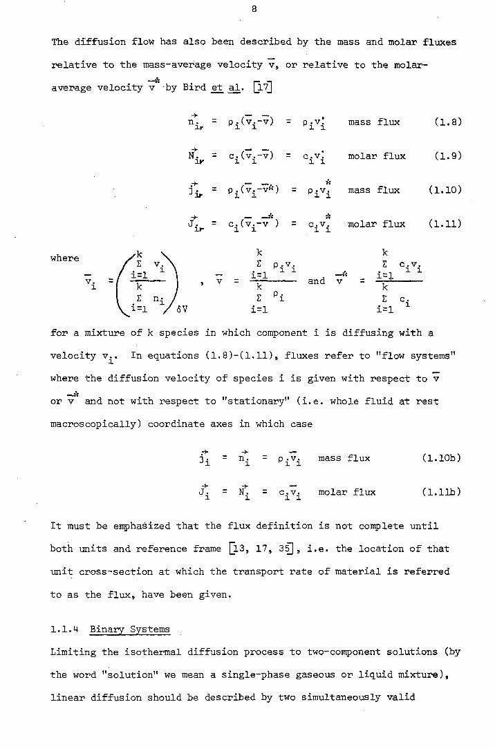
The diffusion flow has also been described by the mass and molar fluxes

relative to the mass-average velocity v, or relative to the molar-

average velocity v by Bird

n^^ = p^(v^-v) = p^v^ mass flux (1.8)

= c^(v^-v) = c^v^ molar flux (1.9)

= Pj,(v^-v«) = p^v^ mass flux (1.10)

— •! .3% A = c^(v^-v ) = molar flux (1.11)

where /!: \ z p .v. J o.v.

V . =1 ^ I . V = and v' =

z ^i S c. SV i=l i=l

for a mixture of k species in which component i is diffusing with a

velocity v^. In equations (1.8)-(l.11), fluxes refer to "flow systems"

where the diffusion velocity of species i is given with respect to v

or V and not with respect to "stationary" (i.e. whole fluid at rest

macroscopically) coordinate axes in which case

= n^ = p^v^ mass flux (l.lOb)

= c^v^ molar flux (1.11b)

It must be emphasized that the flux definition is not conplete until

both units and reference frame [l3, 17, 3^, i.e. the location of that

unit cross-section at which the transport rate of material is referred

to as the flux, have been given.

1.1.4 Binary Systems

Limiting the isothermal diffusion process to two-component solutions (by

the word "solution" we mean a single-phase gaseous or liquid mixture),

linear diffusion should be described by two simultaneously valid

equations, regarding the flow of the two components in opposite

directions:

^1 = -»i inr (1-12)

" 2 = "^2 T T • (1-13)

where the subscripts 1 and 2 in the flux, concentration and diffusion

coefficient refer to the first and second component respectively.

The discussion of diffusion is simplest, hence very important to the

experimentalist, when the reference plane is defined so as to make the

two diffusion coefficients identical with each other [13, 35-3?].

This can be achieved by referring the diffusion flow to that plane where

the change in volume due to the two-directional mass flow crossing the

plane compensate each other, i.e. across this plane there is iw 'transport

of volume'. If the partial molar volumes of the two components are

and Vg and and are the fluxes measured with respect to the 'volume

frame of reference', we have:

+ JgVg = 0 (1.14)

Introducing the fluxes from equations (1.12) and (1.13) and denoting

the diffusion coefficients related to this reference frame by and

Dg, we obtain:

1.1.5 Binary Diffusion Coefficient

According to the definition of the molar volume:

V^c^ + VgCg = 1 (1.16)

and c^6V^ + CgGVg = 0 (1.17)

10

It therefore follows that:

V ^ l VgdCg = 0 (1.18)

Taking this into account, it follows from equation (1.15), that the two

diffusion coefficients must be equal

= Dg = D^2 (1.19)

and thus the subscripts and superscripts in (1.19) may be deleted since

a binary system may be described by a single "mutual-", "inter-" or

"binary-" diffusion coefficient This is often practically equal

to the diffusion coefficient determined experimentally by performing a

diffusion process in which two dilute solutions of different concentra-

tion diffuse towards each other through an initially sharp horizontal

boundary |j-3^ •

1.1.6 Binary-, Self-, and Tracer-Diffusion Coefficients

As indicated earlier, the diffusion coefficient termed mutual or

binary diffusion coefficient and refers to the diffusion of one consti-

tuent in a binary system. A similar coefficient, would imply the

diffusivity of component 1 in a mixture [l7, 36-3^. Experiments

indicate that Pick's first law is not always sufficient to describe

the solute flows in multicomponent systems. Hence, more generalized

diffusion equations have been developed by Onsager [ll]£l , Kirkwood and

Dunlop et al', [36-39]]. Their analyses led to equations and correlations

Involving various diffusivities, namely binary-, self- and tracer-dif-

fusion coefficients.

Tracer-diffusion coefficients (also referred to as intra-diffusion coef-

ficients) relate to^ the diffusion of a labelled component within a homo-

geneous mixture. That is, the component present in traces in the solution

11

has a concentration gradient, while the concentration gradient of all the

other components of high concentration in comparison with the former is

zero. In general, the tracer-diffusion coefficient of a pure liquid is

obtained by adding a small number of radioactively-labelled molecules of

the same substance and allowing them to diffuse into a sample with a

lower concentration of the labelled species. If the molarity of the

labelled species at any point is c?% then it follows from equation (1.6)

A that the tracer-diffusion coefficient D" is defined

^ (1.20)

similarly, the diffusion of labelled molecules or of ions in a solution

of the same, unlabelled, species can be followed and a tracer-diffusion

coefficient, defined by equation (1.20), measured. The smaller the dif-

ference in properties between the labelled and unlabelled species the

closer the experimental tracer-diffusivity approximates to the true

self-diffusion coefficient [isQ. Like binary-diffusion coefficient

(D^g), tracer-diff us ivity (D"') can depend on the concentration [6, 13a,

32] .

The tracer-diffusivity in a pure fluid represents the closest practical

approach to the measurement of the self-diffusivity of the fluid. The

self-diffusion coefficient, is the transport property characteristic of

the hypothetical process in which molecules of one species diffuse

through themselves (i.e. interdiffusion of identical molecules). Evi-

dently, this quantity can never be measured experimentally. Conse-

quently it has sometimes been assumed that the tracer-diffusion coef-

ficient is identical with the self-diffuion coefficient. Such an assum-

ption is not justified and gives rise to the so-called isotope effect

which describes the dependence of the tracer-diffusivity on the particular

12

isotope used for its measurement [32, 40-4^. Tracer-, and self-

diffusion coefficients may also be defined for mixtures of fluids.

In a binary mixture, there are two tracer-, and two self-diffusion

coefficients, one each for the two species. The two tracer-diffusion

coefficients correspond to measurements of the diffusion of one

labelled species in the mixture.

The various diffusion coefficients described above are shown by

Fig. 1.1 which refers to the experimental results for n-octane (.1)/

n-dodecane (2) at 60°C, due to Van Geet et .

Fig. 1.1 - Binary-, self-, and tracer-diffusion coefficients D22 and Dg respectively

Diffusion Coefficient

1 •

0 X2, mole fraction of n-dodecane 1.0

In this case, the binary diffusion coefficient, D22 decreases as the

mixture becomes richer in n-dodecane (2). As Xg ^ 1.0, ~ ^21 ^12

the limiting diffusion coefficient (or intrinsic diffusivity D^) when

the mixture essentially consists of n-dodecane, i.e. n-octane (1)

13

molecules diffusing through almost pure n-dodecane. Similarly,

is the diffusivity of n-dodecane in essentially pure n-octane. It is

useful to note that as Xg 0, i.e. 1.0, the intra-diffusion coef-

o

ficient (Dg) tends to the limiting inter-diffusion coefficient

When Xg ^ 1.0, Dg Dgg, i.e. the tracer diffusion coefficient tends

to the self-diffusion coefficient of pure n-dodecane.

1.1.7 Chemical Potential Driving Force

The 'driving force' of diffusion is the chemical potential gradient Vii .

However, the changes in chemical potential are determined by the changes

in concentration in ideal mixtures

( U i ) 0 - = RT £n X. (1,20a)

But, for real mixtures, the changes in activity a^ must be applied

- ^^i^T,P ^ . = RT &n a^ = RT Hn yY x. (1.21)

" . th where is the activity coefficient of the i component at a given

point in the mixture. In real mixtures, the activity coefficient depends

on the nature and concentration of all of the components. In multi-

component systems, it can occur that the direction of the activity

gradient of a component does not coincide with that of its concentration

gradient and so the component will diffuse from regions of lower con-

centration towards those of higher ones. This often happens in the

course of diffusion through an interface of different phases in hetero-

geneous systems, since the requirement of equilibrium between different

phases containing a given substance is its identical activity (or

identical y). Thus, solutes often diffuse through interfaces towards

points of higher concentration and an example of this is the diffusion

14

of iodine, at the interface of chlorofbmnand water, into the chloroform

solution of higher concentration. In this respect, there is apparently

an essential difference between diffusion and heat conduction although

they are rather similar in a phenomenological sense. Thermal energy

is always transported in the direction of decreasing temperature, and

this applies to its transport through interfaces too. In each case the

requirement for equilibrium is the identical temperature at every point

of the system. As for diffusion, the concentrations are usually dif-

ferent at the two sides of the interface even after reaching the equilib-

rium state.

In diffusion, the gradient of chemical potential and not that of concen-

tration is the analogue of temperature gradient in heat conduction.

However, since there is no instrument which directly measures the

chemical potential or the absolute value of activity, attention is

focussed upon concentration gradients for all practical purposes.

In binary systems where the chemical potential is related to activity

by equation (1.21), all modem theories of diffusion [T] lead to an

activity-corrected diffusion coefficient ^2'

[(9 £n a )/(9 £n )] (1.22)

T,P

where -^2 often less sensitive to composition than ]%] .

1.1.8 The Phenomenological Equation of Diffusion in Irreversible Thermo-dynamics

Because of the irreversibility of the transport phenomena, their

relationships cannot be deduced from classical thermodynamics which

only deals with equilibria and reversible processes. The thermodynamics

of irreversible processes has shown a marked development, initiated by

Onsager, De Groot and Prigogine [lib, 13, 4: , in the last fifty years.

It is now well-known that the rate of entropy production of component i.

15

dSj^/dt, arising from irreversible processes within a system can be

written in the form of a sum of products of generalized fluxes j\ with

generalized forces giving rise to flows

ds. ^ <!> = T J. X. (1.23)

Here represents the dissipation function [l3^.

According to the phenomenological laws of Fourier (for heat conduction).

Ohm (for electrical conduction) and Fick (for diffusion), the correlation

between the fluxes (J^) of heat, electricity or mass and the forces (X\)

giving rise to them is linear. This is shown experimentally to be true

when a system is close to equilibrium, otherwise the correlation is a

power series in X^. The linear relationship is basically the so-called

Onsager linear law (verified by the Bearman-Kirkwood statistical mecha-

nical theory of transport process {44, 4-^), given by the phenomeno-

logical equation

^i " -^i i (1.24)

where it is assumed that X^ is the only force acting on the i^^ component

->• A

to cause the flow J^. In this equation, is the phenomenological coef-

ficient of flow [1^. In an isothermal non-electrolytic system, the

thermodynamic force X^ resulting in diffusion of the i"*" component is

the gradient of chemical potential [lib, 43^.

Hence equation (1.24) becomes:

X^ = - V (1.25)

(i = 1, 2, 3 ...)

= - lit V (1.26)

Equations (1.23) and (1.26) clearly indicate that the rate of entropy

production of species i depends on the dissipation of the chemical

16

potential gradient of i. The comparison bf equation (1.26) with (1.2)

shows that the diffusion flux can be related to either the dissipation

of a concentration, or chemical, potential gradient.

In general, if several other thermodynamic forces X^, ... (e.g.

gradients of temperature, electrical charge, etc.) simultaneously

influence the i^^ component of a thermodynamic system, then the transport

of i due to its chemical potential gradient would be affected by such

forces, referred to as the 'hross-effects" [l3]] , and its flux will be

given by

^ ^ A J. = Z L X, (1.27) ^ k=l

The phenomenological coefficients of the cross-effects are "symmetrical"

according to the Onasger reciprocity theory

This theory can be easily understood by a simple example. Consider a

binary solution in which there is temperature and composition varia-• —

tions. The fluxes J of mass flow and J, of heat flow are determined m h

by the chemical potential gradient X^ and the temperature gradient Xg

s imultaneously.

4- A A , . J = L X + L , X, mass (1.29) m mm m mh n

f = l'V X, + l'' X heat (1.30) h hh h hm m

it A

where and are the phenomenological coefficients corresponding

to the effect of chemical potential gradient on mass transport in dif-

fusion and that of temperature gradient on heat transport, respectively. :V

Of the cross-effects, is the phenomenological coefficient corres-

ponding to the effect of the temperature gradient on mass transport.

1 7

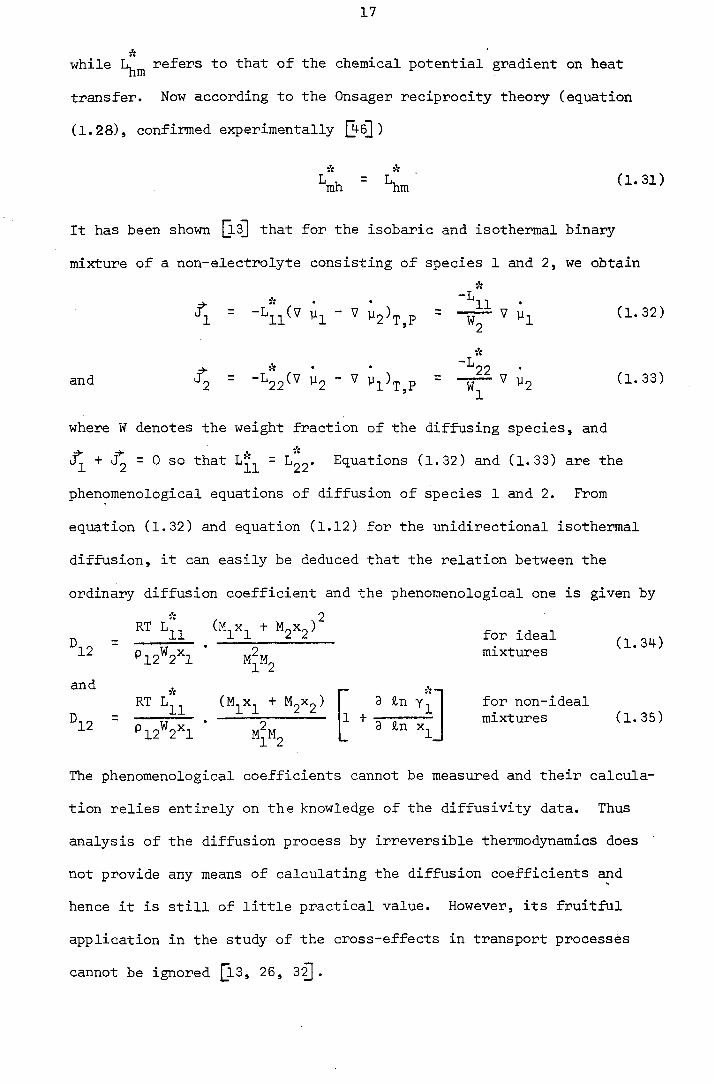
while refers to that of the chemical potential gradient on heat

transfer. Now according to the Onsager reciprocity theory (equation

(1.28), confirmed experimentally [4^)

4 = C It has been shown Q.3 that for the isobaric and isothermal binary

mixture of a non-electrolyte consisting of species 1 and 2, we obtain

A

JJ_ - - V ^ 2 ^ T , P ~ ~ W ^ ^ ^ 1 ( 1 . 3 2 )

l'

and ^2 " " 22'' 2 ~ ^ ^l^T P ~ ~ W ^ ^ ^2 (1.33)

where W denotes the weight fraction of the diffusing species, and

+ >^ = 0 so that = ^22' Equations (1.32) and (1.33) are the

phenomenological equations of diffusion of species 1 and 2. From

equation (1.32) and equation (1.12) for the unidirectional isothermal

diffusion, it can easily be deduced that the relation between the

ordinary diffusion coefficient and the phenomenological one is given by

D = ideal 12 P12^2^1 mixtures

and a RT (M^x^ + MgXg)

12 P12^2^1

9 &n

^ ^ 9 &n x^

for non-ideal mixtures (1.35)

The phenomenological coefficients cannot be measured and their calcula-

tion relies entirely on the knowledge of the diffusivity data. Thus

analysis of the diffusion process by irreversible thermodynamics does

not provide any means of calculating the diffusion coefficients and

hence it is still of little practical value. However, its fruitful

application in the study of the cross-effects in transport processes

cannot be ignored [l3, 26, 3^ .

18

1.2 MODELS FOR DIFFUSION IN LIQUIDS

In principle, the theory of statistical mechanics of liquids [4'^ should

enable any process in liquids, including the transport processes, to

be described in terms of the motion and properties of the atoms and

molecules which make up the liquid. But in practice, this approach has

so far not been developed to the point where the diffusion coefficient

may be calculated for a real fluid without further approximations.

Frequently these approximations take the form of a model of the liquid

and the motion of its molecules. Recently it has become possible to

assess the validity of some of these models of liquids by means of

molecular dynamics simulations and they have often been found to be

unsatisfactory [4^• Nevertheless, the approximate theories are often

all that is available for the calculation and correlation of diffusion

coefficients of liquids so that there is little doubt that they will be

in common use for some time to come. In some cases, the approximate

theories yield relationships between diffusion coefficients and the

properties of a system with considerable value for estimation purposes.

For these reasons we consider here first the approximate models of dif-

fusion in liquids and postpone a discussion of the current state of

the rigorous statistical mechanical theory until later.

In general, the models for diffusion in liquids can be classified into

three groups:

(1) Hydrodynamic models - based on the Stokes-Einstein analysis.

(2) Kinetic models - due to Eyring and other investigators.

(3) The van der Waals model.

19

1,2.1 The Hydrodynamic Model for Diffusion

The hydrodynamic model of diffusion Q.a, 13a, 32, 4 ^ considers the

liquid as a continuum in which the transport of a component is deter-

mined by the resultant of the driving force and the frictional resis-

tance force acting upon it. As mentioned in our earlier discussions, the

gradient of chemical potential is the driving force. (In old theories,

due to Sutherland and Einstein [49, 5( , the gradient of osmotic pres-

sure was considered as the driving force). If species 1 dissolves in

liquid 2 and an ideal mixture is formed on dissolving, then from

equation (l.20a), we have

5 1 9 an c 9c

-jt -- --

where is the chemical potential gradient of the solute (the

measure of the driving force of diffusion) in the z direction. If f^

is the frictional force of resistance of the solute per molecule (i.e.

Nf per mole), the average velocity of one-dimensional diffusion is

According to hydrodynamic considerations and from equations (1.5) and

(1.11b), the binary diffusion coefficient is therefore given by

= eAl. KT (1.38) s

where is the mobility of the solute particles (i.e. their velocity

gained as a result of unit force). This is the so-called "Nernst-

Einstein equation" [l" . The most difficult, and still not reliably

solved, problem which arises in the hydrodynamic theory is the calcula-

tion of the frictional resistance from other properties of solutions.

This is due to our inadequate knowledge of the liquid structure. Con-

20

sequently, the diffusion coefficient calculated from other properties

of a solution is not accurate since the assumptions applied in evaluating

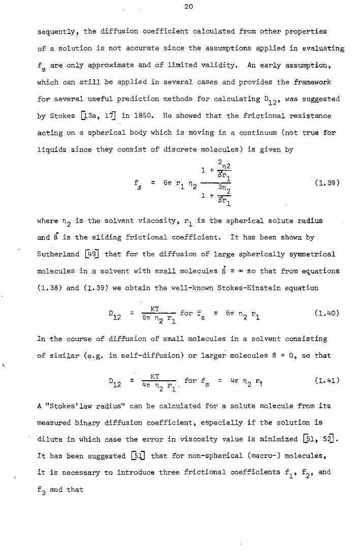
fg are only approximate and of limited validity. An early assumption,

which can still be applied in several cases and provides the framework

for several useful prediction methods for calculating was suggested

by Stokes [l3a, ifj in 1850. He showed that the frictional resistance

acting on a spherical body which is moving in a continuum (not true for

liquids since they consist of discrete molecules) is given by

= S" "2 a T (1-39)

where rig is the solvent viscosity, r^ is the spherical solute radius

and 3 is the sliding frictional coefficient. It has been shown by

Sutherland Qt- that for the diffusion of large spherically symmetrical

molecules in a solvent with small molecules B = <» so that from equations

(1.38) and (1.39) we obtain the well-known Stokes-Einstein equation

KT

"l2 = 6, ng "2 ''l

In the course of diffusion of small molecules in a solvent consisting

of similar (e.g. in self-diffusion) or larger molecules 3 - 0, so that

KT ®12 = '1

A "Stokes'law radius" can be calculated for a solute molecule from its

measured binary diffusion coefficient, especially if the solution is

dilute in which case the error in viscosity value is minimized [si, 5^.

It has been suggested [si] that for non-spherical (macro-) molecules,

it is necessary to introduce three frictional coefficients f^, f^, and

f2 and that

21

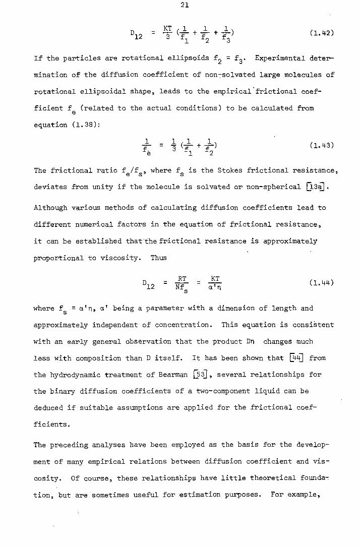
°12 = (1.42)

If the particles are rotational ellipsoids f^ = f^. Experimental deter-

mination of the diffusion coefficient of non-solvated large molecules of

rotational ellipsoidal shape, leads to the empirical frictional coef-

ficient f (related to the actual conditions) to be calculated from

e

equation (1.38):

^ = I ( ^ + ) (1.43)

^e ^1 ^2

The frictional ratio f^/f^, where f^ is the Stokes frictional resistance,

deviates from unity if the molecule is solvated or non-spherical [l3^.

Although various methods of calculating diffusion coefficients lead to

different numerical factors in the equation of frictional resistance,

it can be established that the frictional resistance is approximately

proportional to viscosity. Thus

"12 = ^ ^

where f^ = a'n, oi' being a parameter with a dimension of length and

approximately independent of concentration. This equation is consistent

with an early general observation that the product Dn changes much

less with composition than D itself. It has been shown that [4'+] from

the hydrodynamic treatment of Bearman , several relationships for

the binary diffusion coefficients of a two-component liquid can be

deduced if suitable assumptions are applied for the frictional coef-

ficients.

The preceding analyses have been employed as the basis for the develop-

ment of many empirical relations between diffusion coefficient and vis-

cosity. Of course, these relationships have little theoretical founda-

tion, but are sometimes useful for estimation purposes. For example,

22

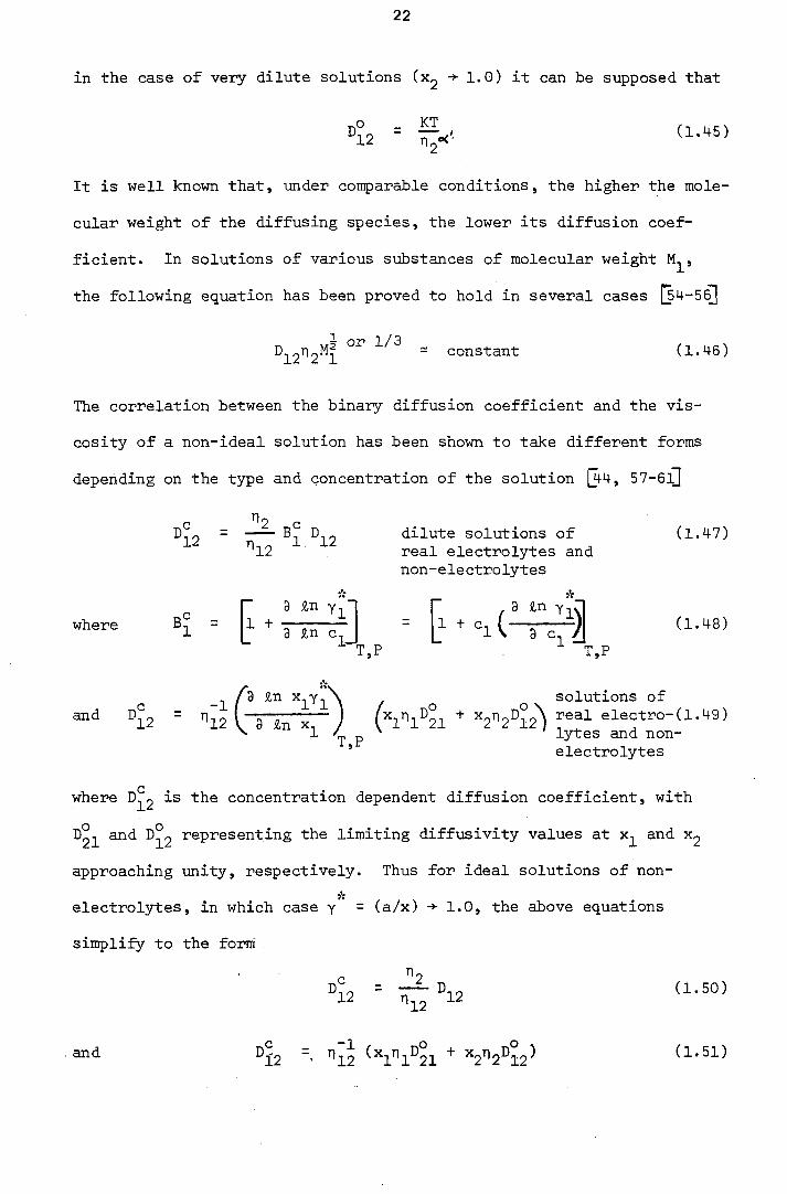
in the case of very dilute solutions (x^ 1.0) it can be supposed that

It is well known that, under comparable conditions, the higher the mole-

cular weight of the diffusing species, the lower its diffusion coef-

ficient. In solutions of various substances of molecular weight

the following equation has been proved to hold in several cases [^4-5^

^12^2^1 - constant (1.4-6)

The correlation between the binary diffusion coefficient and the vis-

cosity of a non-ideal solution has been shown to take different forms

depending on the type and concentration of the solution [44, 57-6l]

c ^2 c , D^2 - dilute solutions of (1.47)

^12 real electrolytes and non-electrolytes

where

T,P T,P

-1 ** *lYl' I *2^2^12) T . P

electrolytes

r / 9 Jin Yi \ f solutions of

"12 = "12 i 3 to K., J (*l"lD21 + real electro-(1.49) \ T P lytes and non-

where is the concentration dependent diffusion coefficient, with

D°2 and representing the limiting diffusivity values at and Xg

approaching unity, respectively. Thus for ideal solutions of non-

electrolytes, in which case y = (a/x) -> 1.0, the above equations

simplify to the form

D12 = ^ " 1 2 (I'SO)

and D^2 ^^^1^1^21 ^2^2^12) (l'5l)

23

where ^2 and ri 2 all the above equations denote the viscosities

of the pure solute, pure solvent and the solution respectively. A

number of similar correlations have been recorded in the literature

[3J 13a, . However, the experimental results of Van Geet et al.

( [3^ ; n-ocante/n-dodecane mixture) and King et a2. ( ; glycol/water

mixture) can provide a way of determining the validity of any such cor-

relations. According to their empirical findings

~ ^1^21 ^ ^2^t2 Van Geet et al.(1.52)

( 12 12 \ i f(T) King et al. (1.53) = f(c)

Equation (1.52) has been varified empirically by a number of investi-

gators [58, 121^ .

1.2.2 Kinetic Models of Diffusion

Although certain relationships have been revealed by various treatments

of the hydrodynamic model of diffusion, none of the analyses provide a

deeper understanding of the molecular mechanism of the phenomenon. This

is because they regard the liquid as a continuum and neglect its mole-

cular structure. The kinetic statistical models, such as that of Eyring

et [63-65]] assume a molecular mechanism of diffusion. The particular

model of molecular motion embodied in the Eyring theory has recently

been shown to be incorrect [48, 66^. Nevertheless, its widespread use

makes it necessary to discuss it and many of its qualitative predictions

are in reasonably good agreement with experimental observations [62]] .

The theory is based upon a relatively simple model of the liquid state

(i.e. spherically symmetric, monatomic, molecules such as those of

liquefied rare gases and alkali metals) and leads to the derivation of

an expression for the diffusion coefficient by applying the theory of

24

absolute reaction rates. It assumes that the diffusion can be described

in a similar fashion to the rate processes of mono-molecular reactions,

involving a temporary configuration of the species which can be con-

sidered as an intermediate activated state. The mechanism of diffusion

is, in many respects, similar to that of viscous flow, except that

unlike molecules are involved in the former process. In solution,

diffusion requires the slipping of the solute and solvent molecules past

one another. In the course of their movement, solute molecules should

cross the potential barrier (free enthalpy barrier) separating two

adjacent equilibrium positions in the liquid structure. If \ is the

distance between the two equilibrium positions, then the molecules

cover this distance in each jump in the direction of decreasing con-

centration. Because the standard free enthalpy of ideal solutions is

identical in all equilibrium positions occupied by the diffusing mole-

cules, then, assuming a symmetrical energy barrier, the free enthalpy

of activation of the process in the direction of decreasing concent-

ration must be identical to that in the opposite direction. In other

words, the forward (diffusional) and backward (thermal) rates of mole-

cular transport are equal. Consequently, the specific rate constants of

the process in the two directions are equal to each other (k^ = k^ = k).

It can easily be shown [32 that the actual rate of one-dimensional

diffusion (i.e. the resultant velocity of the solute molecules) is given

by

— — — c\r . V = v^ - Vy = -NX k (1.54)

dc = -DN according to

Pick's law

and hence by comparison

*2 D = X k (1.55)

25

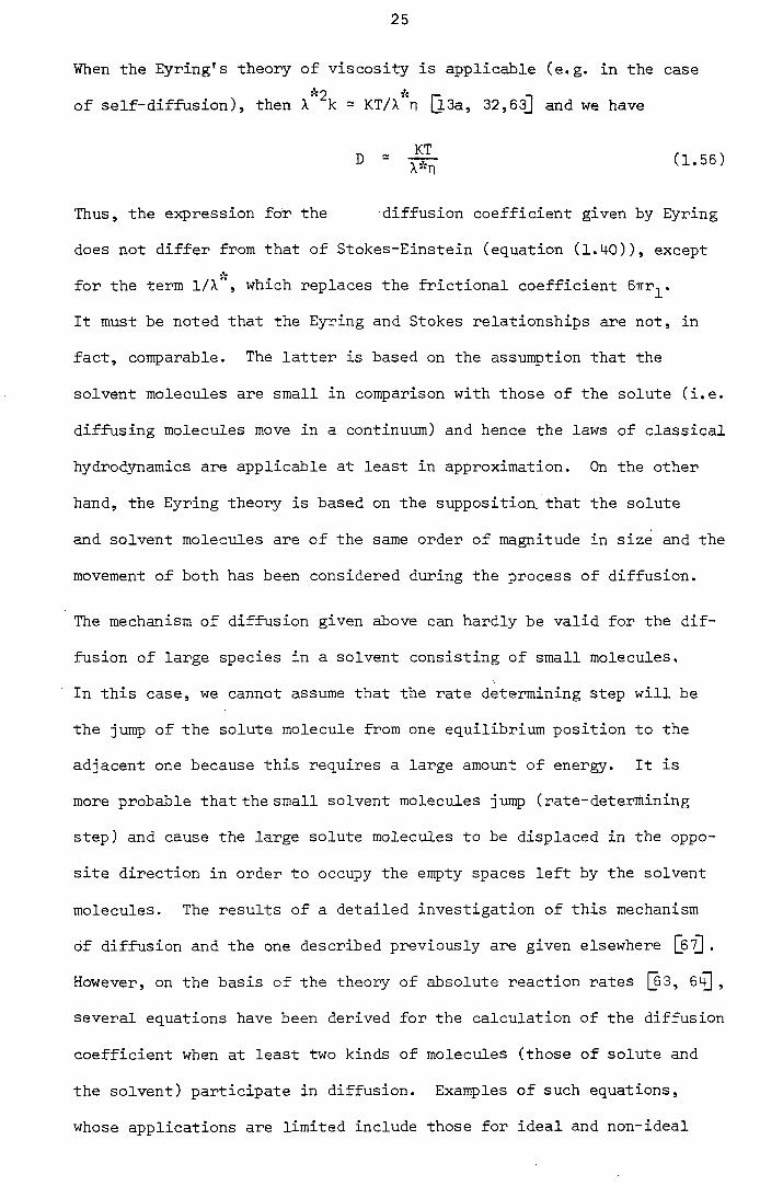
When the Eyring's theory of viscosity is applicable (e.g. in the case

of self-diffusion), then X = KT/X n [l3a, 32,63j and we have

KT D • ^ (1.56)

Thus, the expression for the diffusion coefficient given by Eyring

does not differ from that of Stokes-Einstein (equation (l.i+O)), except

for the term 1/X , which replaces the frictional coefficient Gnr^.

It must be noted that the Eyring and Stokes relationships are not, in

fact, comparable. The latter is based on the assumption that the

solvent molecules are small in comparison with those of the solute (i.e.

diffusing molecules move in a continuum) and hence the laws of classical

hydrodynamics are applicable at least in approximation. On the other

hand, the Eyring theory is based on the supposition., that the solute

and solvent molecules are of the same order of magnitude in size and the

movement of both has been considered during the process of diffusion.

The mechanism of diffusion given above can hardly be valid for the dif-

fusion of large species in a solvent consisting of small molecules.

In this case, we cannot assume that the rate determining step will be

the jump of the solute molecule from one equilibrium position to the

adjacent one because this requires a large amount of energy. It is

more probable that the small solvent molecules jump (rate-determining

step) and cause the large solute molecules to be displaced in the oppo-

site direction in order to occupy the empty spaces left by the solvent

molecules. The results of a detailed investigation of this mechanism

of diffusion and the one described previously are given elsewhere [6?].

However, on the basis of the theory of absolute reaction rates [63, ,

several equations have been derived for the calculation of the diffusion

coefficient when at least two kinds of molecules (those of solute and

the solvent) participate in diffusion. Examples of such equations,

whose applications are limited include those for ideal and non-ideal

26

binary solutions [32, 6 ^

D = 1/3 2irm

ideal solution

(1.57)

where is the liquid-free volume [6^ and m - /m^+mg is the

reduced mass of two types of molecules,

A , X

D solute

'r73. 75l

solution

/a 2n ^

• Y in xj. solute

or Dn

^ d In a\ \Jb &n X j

= A KT (1.58)

3 Jin X

This equation is in good agreement with the experimental results for

the chloroform-ether mixture [S^ as shown in Fig. 1.2.

Fig. 1.2 - Variation of Dn and Dn/O &n a/3 £n x) with concentration

in chloroform-ether mixture

2,0 -

1-5 .

10

Vc

ckUrofai irm 5oZ etktr

27

Thus J according to equation (1.58), the product Dn has a maximum in

agreement with the experimental data. Similar results have been obtained

for other mixtures whose activities could be determined by measuring

the partial vapour pressures proportional to the activities.

In view of the fact that the Eyring theory has now been discredited

[48, 6 ^ , it is not surprising that marked deviations can be observed

between the calculated and measured values of some properties such as -

the diffusion coefficient [ 32, 48, 6^. This is because the theory in

its details is based on very simple assumptions, and more or less,

reliable conclusions could be drawn from it only for the main features

of diffusion. The theory has been extended and modified to eliminate

its deficiencies by several workers [e.g. 6^. In addition, several

other molecular theories such as the theory of transfer diffusion [j( ,

(based on the assumption that diffusion is due to a molecular exchange

of reactions as well as migration to lower concentration regions),

Panchenkov theory [jl], (based on van der Waals/Maxwell analyses - a

molecule will diffuse (a) if it has gained sufficient kinetic energy

to break the van der Waals bonds with its neighbours (b) if adjacent

molecules are sufficiently far apart for the diffusing molecule to pass

between them), Frenkel et ad. theory [j^ , (the onset of diffusion is

considered to be the rotational and vibrational motion due to collisions

in a liquid containing dipole molecules) and the theory of Jensen et al.

[jd , (based on time-dependent correlation functions, the diffusion

coefficient and viscosity are correlated through such functions) have

been proposed. Unfortunately, all such attempts have failed to produce

a satisfactory theory of diffusion.

28

1.2.3 The van der Waals' Model

Although the van der Waals' model has proved to be of great value for

calculation of density dependence of self-diffusion coefficients, it

has not so far been of great value to the description of the temperature

and concentration dependence of binary diffusion coefficients.

Conguter simulation studies by the method of molecular dynamics (Section

1.3.4) have now discredited the Eyring activation energy model for dif-

fusion in liquids. The studies also reveal that the effect of the attrac-

tive part of the intermolecular potential energy function is far less

significant than is postulated in the Brownian motion approximation

(Section 1.3.2). Indeed, they prove that the van der Waals' model is

a better approximation even under ordinary liquid conditions. The

findings of this model and molecular dynamics simulations are often

similar and very valuable in the study of the transport properites and

hence attaching a significant importance upon the model and the results

described here, even though they are limited to pure fluids. In fact,

it will be seen later on that recent efforts, based on molecular

dynamics simulations, to extend the rough hard sphere theory for pure

fluids to binary systems depend on the transport property data for the

pure fluids.

The van der Waal^ model of a fluid considers the molecules to have an

intermolecular potential made up of a hard core surrounded by a weak,

long-range attractive component [j4-, 75 . For a system of such mole-

cules, the well-known van der Waal^ equation of state is rigorously

obeyed . For real fluids the intermolecular potential does possess

a steep repulsive wall, although not infinitely steep, and the range

of the attractive forces is large relative to the intermolecular spacing

at densities higher than the critical density. Furthermore, the attrac-

29

tive potential may be considered weak relative to the kinetic energy

whenever the temperature is greater than the well-depth (or =0.7 times

the critical temperature). As a result for relatively high temperatures

and densities, real fluids obey the van der Waals' equation of state

quite well , provided that the core size is allowed to decrease as

the temperature increases to reflect the finite steepness of the

repulsive wall of the potential .

From the point of view of the transport properties of dense fluids, the

van der Waals' model is consistent with the findings of molecular dynamics

simulations (see Section 1.3.4) in that the molecules move very nearly in

straight lines between hard core collisions; because at high densities

the attractive potential forms a uniform surface Qs]. The description

of the van der Waals' model indicates that it should be most accurate

at high densities and high temperatures, i.e. at the very dense gas

region. But it has also been successfully applied to liquids, and even

extended to lower densities where perturbation theory may be used to

account for the increasing influence of attractive forces [79 . Under

conditions of high density and temperature, the van der Waals'model

allows the transport properties of monatomic fluids to be described by

the Enskog smooth rigid sphere theory which has been treated in detail

by Chapman e^ a_l. [soj . Basically, the assumption is made that the

fluid consists of hard spheres and behaves like a low-density hard

sphere (Boltzmann analysis) system except that all events occur at a

faster rate due to the higher rate of collision [81, 82] . The transport

coefficients for the dense fluid may thus be written in terms of their

dilute gas values. For example, the ratio of the self-diffusion coef-

ficient Dg, valid at high number density n",to that at low density n^,

denoted by is given by [ Cl

n*Dp ^ (1-59) o o

30

where is the radial distribution function [lb,c,d] at contact for

spheres of diameter and depends on the co-volume b. In oi?der to

employ equation (1.59) for the calculation of the diffusion coefficients

it is necessary only to find gfa^) and a suitable value for the co-

volume b. In the original application of this method b was obtained

by fitting the PVT data for the noble gases to the van der Waals' equation

of state and g(Op) was taken from the results of computer simulations

[74]. It was found that the calculated high density transport coef-

ficients differed by less than 10% from the experimental values.

However, the Enskog theory neglects all correlations of molecular velo-

cities in the evaluation of the transport coefficients (e.g. the

Enskog expression for dense fluid diffusion based on the molecular chaos

approximation). Because the computer simulations indicate their exis-

tence and the van der Waals' model allows them, an improved calculation of

the transport properties is possible when they are included [7^.

Molecular dynamics simulations, of the type described in Section 1.3.4,

have been employed to deduce the corrections to the Enskog theory which

arises from velocity correlations for smooth hard spheres [79]]. For

instance, the correction for self-diffusivity, in the form of ratios of

the exact hard sphere, result to the Enskog result, may be written as

0 0 o E

is related to the number density at temperature T by

where m is the mass per molecule. It has been found that the correction

is largest for self-diffusivity and it amounts to an increase of about

35% at densities 1.5 to 2 times the critical density, but to a decrease

of about 40% as solidification is approached. On the other hand.

31

thermal conductivity corrections show a weak dependency upon the

density, never exceeding 10%.

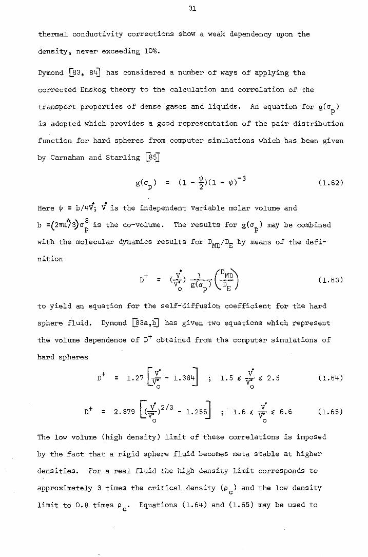
Dymond [83, 8^ has considered a number of ways of applying the

corrected Enskog theory to the calculation and correlation of the

transport properties of dense gases and liquids. An equation for gCa^)

is adopted which provides a good representation of the pair distribution

function for hard spheres from computer simulations which has been given

by Camahan and Starling [sCI

g(cJp) = (1 - 0(1 - (1.62)

Here ^ = b/M-V; V is the independent variable molar volume and

b =^2Tm7^o^ is the co-volume. The results for gCo^) may be combined

with the molecular dynamics results for by means of the defi-

nition

to yield an equation for the self-diffusion coefficient for the hard

sphere fluid. Dymond [ [ 8 3 a h a s given two equations which represent

the volume dependence of obtained from the computer simulations of

hard spheres

D+ = 1.27-^-1.384] ; 1 . 5 ^ - ^ ^ 2 . 5 (1.64) ^ o —' o

. 379 - 1.256^ ; 1.6 ^ ^ 6.6 (1.65) D"*" = 2

The low volume (high density) limit of these correlations is imposed

by the fact that a rigid sphere fluid becomes meta stable at higher

densities. For a real fluid the high density limit corresponds to

approximately 3 times the critical density (p^) and the low density

limit to 0.8 times p^. Equations (1.64) and (1.65) may be used to

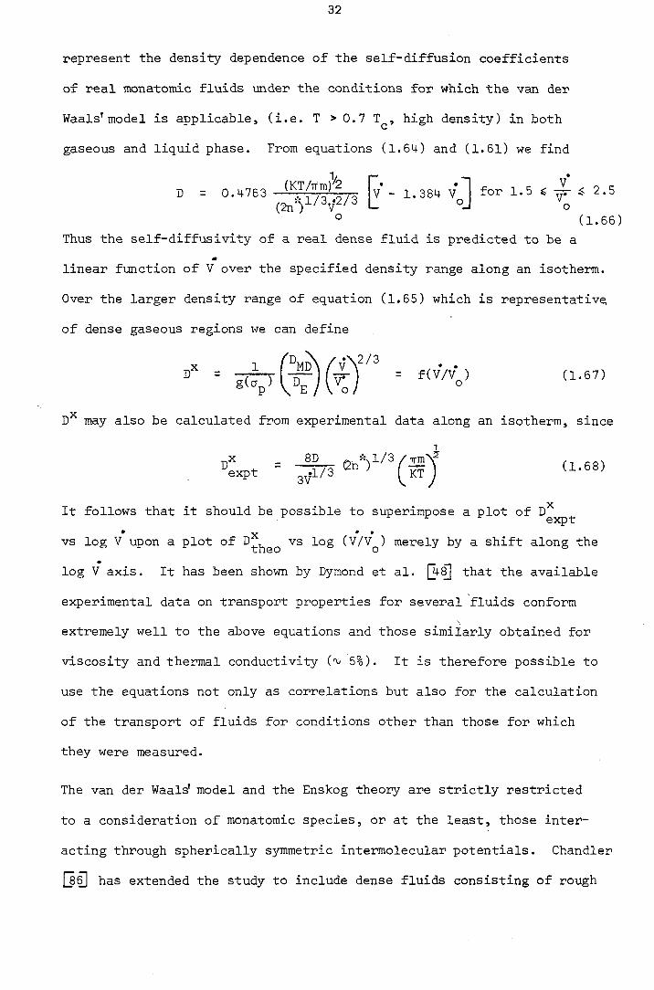
32

represent the density dependence of the self-diffusion coefficients

of real monatomic fluids under the conditions for which the van der

Waals'model is applicable, (i.e. T >0.7 T^, high density) in both

gaseous and liquid phase. From equations (1.64) and (1.61) we find

" = "o] t ° (1.66)

Thus the self-diffusivity of a real dense fluid is predicted to be a

linear function of V over the specified density range along an isotherm.

Over the larger density range of equation (1.65) which is representative^

of dense gaseous regions we can define

may also be calculated from experimental data along an isotherm, since

"Lpt - # 7 3 j (1.S8,

It follows that it should be possible to superimpose a plot of

• X * *

vs log V upon a plot of vs log (V/V^) merely by a shift along the

log V axis. It has been shown by Dymond et al. Qt- that the available

experimental data on transport properties for several fluids conform

extremely well to the above equations and those similarly obtained for

viscosity and thermal conductivity ('\> 5%). It is therefore possible to

use the equations not only as correlations but also for the calculation

of the transport of fluids for conditions other than those for which

they were measured.

The van der Waals' model and the Enskog theory are strictly restricted

to a consideration of monatomic species, or at the least, those inter-

acting through spherically symmetric intermolecular potentials. Chandler

[jCl has extended the study to include dense fluids consisting of rough

33

hard spheres, model for a system in which there is translational"internal

energy coupling through non-spherically symmetrical force fields. He has

shown that [86b] for a rough hard sphere fluid at densities greater than

twice the critical density

^RHS ~ ^ ^SHS (1.69)

where A represents a translational-rotational coupling factor less than

unity which is assumed to be independent of temperature and density.

Thus for the non-spherically symmetric molecules equation (1.66) is

expected to reform to

D = (V _ 1.384 vL) (1.70) y--/ --Vl / .1 V Mill t O

SO that A and may be determined from experimental data-

The rough hard sphere theory of Chandler [vs] Dymond [78, 83(^ for

pure fluids have been extended to binary mixtures by Anderson al.

[^7^ and Bertucci al. [SB] . It has been assumed that the kinetic

diffusion coefficient of a real two-component fluid is given by [89]

" ! >

where is the kinetic binary diffusion coefficient derived by Enskog

for a mixture of hard spheres at the same temperature as the real fluid

and function F depends on the packing factor (J), the appropriate mass

and molecular diameter ratios and the mole fraction of the solvent.

Calado and Castro [s^ have shown that it is possible to obtain the

values of the translational-rotational coupling factor A and the hard

core volumes from the viscosity and self-diffusion data.

34

1.3 THE RIGOROUS THEORY OF THE TRANSPORT PROPERTIES OF DENSE FLUIDS

From the macroscopic point of view the transport properties of a fluid

are those coefficients which give a measure of its tendency to produce

entropy when perturbed from an equilibrium state [l3, 32 . From the

microscopic point of view the entropy production, and hence the values of

the transport coefficients, are a manifestation of the motion of the

molecules which make up the fluid as well as the exchange of energy and

momentum among them. For this reason the transport coefficients are

closely related to molecular motion, to the mechanism of molecular encoun-

ters and thereby to the intermolecular force field. The rigorous molecular

theory of fluids seeks to establish the formal connection between these

microscopic events and the observable transport coefficients. First,

such a connection enables a knowledge of the details of molecular encoun-

ters to be employed to evaluate the transport coefficients. Secondly,

a precise knowledge of the transport coefficients from experiment can be

applied to the verification of the molecular theory itself and of hypotheses

and statements made about the intermolecular potential. Finally, the

molecular theory may reveal relationships among different transport coef-

ficients or between transport coefficients and the parameters of the

thermodynamic state of the fluid Qj-M-, 45, 53, 9( which considerably

reduce the experimental effort required to determine all of the coefficients

over a wide range of states.

So far, one of the most successful theories of this kind has been the

well-known kinetic theory of gases [91-94] which has its origins in the

works of Bernoulli, Clausius, Maxwell and Boltzmann QCl • The simplest

fluid and that for which the kinetic theory is most secure is a dilute

gas composed of identical, monatomic molecules interacting through a

35

spherically—symmetric force field and obeying the laws of classical

mechanics. In view of the difficulties which surround the theory even

in this simple case, it is not surprising that as the system becomes

progressively more complicated, either by virtue of increasing complexity

of the molecules or increasing density, its theoretical description

becomes less secure. For dense gases and liquids, the formal theory is

not yet fully developed and their treatment has proved to be exceedingly

difficult. Thus, although a formal statistical mechanical theory for the

transport coefficients exists [92, 9 ^ , its implementation for calculations

for real fluids has only been accomplished by means of approximations.

These approximations are based on still further models of molecular

motion whose physical basis is uncertain.

1.3.1 Statistical Mechanical Theory

The most complete statistical mechanical description of the behaviour

of a fluid is given by the Liouville equation [lb,c,d, 9l]. This

equation describes the evolution of the N-particle distribution function

f^ in the 6N-dimensional phase space for a fluid of Np particles. The

changes in this distribution function occur because of free molecular

motion and interactions among allN^ particles. The Liouville equation

is based upon classical mechanics and is therefore reversible in time.

This means that if at some instant of time the velocities of all the

particles in the system were reversed, then the particles would retrace

their trajectories in phase space so that all earlier states of the

system in phase space would be recovered.

According to the usual statistical mechanical hypothesis the value of

any macroscopic quantity, a, for a fluid is given by the average of

the corresponding microscopic quantity a(ri^)over the relevant phase

space

36

a(r, t) = /a(rj )fj (r ; t)dr_ (1.72) P P P P

where represents a point in SN-dimensional phase space. With the aid

of the Liouville equation it is then possible to obtain the equations

of change for any quantity a(r\ t), such as the mass, momentum and

energy, in terms of integrals over the N-particle distribution function

[sjQ . These equations represent the statistical mechanical analogues of

the equations of motion for the fluid in terms of the N-particle distri-

bution function. Thus if f^^the distribution function were known, the

equations of motion could be evaluated and the coefficients of the

gradients of the macroscopic variables identified with the transport

coefficients and expressed in terms of the microscopic properties of the

molecules of the fluid.

There are two difficulties encountered in carrying out this programme.

First, a kinetic theory must be established for the function fj^which

involves, in principle, the solution of a dynamic problem involving

particles (the so-called "many-body problem"). Secondly, because the

Liouville equation is reversible it is necessary to somehow introduce

irreversibility into the theory in order that it agrees with practical

experience. In the case of dilute gas the first difficulty is overcome

by simply the rarity of many-body events, whereas the irreversibility

is introduced by the molecular chaos assumption [id, 95]. But for dense

fluids neither of these difficulties has been fully resolved so that it

has been necessary to develop approximate theories [93, 9^. Generally

such theories employ a contracted description of the fluid in terms of

the single-particle and two-particle distribution functions. The intro-

duction of Irreversibility into the theory is then accomplished by a

statistical assumption concerning the lack of correlation in molecular

motion on some macroscopic time scale. In the particular case of the

37

dilute gas the appropriate time scale is the duration of a single

collision, t^^^, but in a dense fluid it may be significantly larger.

1.3.2 The Rice-Allnat Theory

The Rice-Allnat theory [91-9^^ is based upon a model of the fluid for

which it is possible to discern two microscopic time scales. In the

first instance, the theory is applied to spherically symmetric monatomic

species interacting through pairwise additive intermolecular pair

potentials. The model replaces the true intermolecular pair potential by

a rigid repulsive core of diameter surrounded by an arbitrary attrac-

tive potential. In the dense fluid state, the attractive potential is

assumed to contribute to a weak fluctuating background force acting on the

particles. The first time scale of the theory is then associated with

the large momentum and energy transfer which occurs when the hard cores

of two molecules interact. The second time scale corresponds to the

frequent, but small, energy and momentum transfers which occur during

the Brownian-type motion caused by the weak attractive force field. The

hard core collisions are supposed to occur in a time short enough that

no more than binary encounters of this kind need be considered.

The first essential simplification that results from this model is that

the hard core collisions may be treated in the same way as for the;dilute

gas. That is, the Brownian motion between such collisions is supposed

to randomize the velocities of the particles following one hard sphere

collision so that they are uncorrelated before the next. Thus the

changes in the single particle distribution function, f^, which occur

because of hard sphere collisions may be represented by the collision

term of the original Boltzmann equation [le, 9^. The changes in the

single-particle distribution function caused by the Brownian motion

are then treated in an additive fashion. Thus the changes in f^ by

38

virtue of collision are written as [9l]

• ( % •

where the first term is the Chapman-Enskog collision term of the dilute

gas and the second, Fokker-Planck term describes the effects of the

Brownian motion [Tc, 9]] . The separation of the two components in this

equation enables a solution to be obtained for f^ (and also for f^) which

can be used in the statistical mechanical equations of motion to obtain

explicit equations for transport coefficients. The simplest example of

this is the self-diffusion coefficient

D = (1.74)

where f - "3 n"a^gCa^) (irmKTis an effective friction coefficient for

the hard sphere interactions and fg is a friction coefficient for the

Brownian motion. If the Brownian motion is neglected, equation (1.74)

reduces to the Enskog result for a dilute gas of hard spheres undergoing

uncorrelated collisions. In the more general case, the determination of

fg requires a calculation based on molecular statistical dynamics for

which a further model must be introduced. Of all the models suggested

for this purpose none is satisfactory [91, 92^.

The model of molecular motion upon which the Rice-Allnat theory is based

has been challenged by the results of molecular dynamics simulations of

liquids (Section 1.3.4; [66, 92, 97, 98]). In these calculations, the

classical equations of motion for an assembly of particles are solved

numerically so that it is possible to follow the motion of individual

molecules and groups of molecules in the simulated liquid. These

computer simulations show that the soft and hard collisions occur in

roughly equal proportions [66] and hence there is not a large majority

39

of soft collisions as implied by the Rice-Allnat model. Calculations of

transport coefficients of liquefied noble gases based on this model have

generally been in poor agreement with experimental results ^1, 9^] , It

has not yet been established whether this is due to incorrect modelling

of the molecular motion or poor radial distribution functions and inter-

molecular potentials for the liquid.

1.3.3 Method of Time Correlation Functions

An alternative method of formulating the transport coefficients of dense

fluids is provided by the fluctuation dispersion theorem Qi, 43^.

This theorem relates a correlation function for spontaneous fluctuations

in a system in stationary state to the dissipation (or, in thermodynamics

terms, entropy production) of the system under the influence of time

dependent driving forces. If the time dependent driving forces are the

concentration (chemical potential in thermodynamics terms), flow velocity

or temperature, it is possible to express the corresponding transport

coefficients in terms of auto-correlation functions of microscopic

fluxes [lb, <r] . Thus the self-diffusion coefficient of a fluid is written

in terms of the- velocity auto-correlation function as [99, 10(^

1 " D = - / <v.(0) . v.(T)>dT (1.75)

3 Q -1 -1

where v^(0) and V^(T) are the velocities of the molecule i at time zero

and some later time x, respectively. The angle brackets denote an

ensemble average of the quantity, using an N-particle distribution function

for the unperturbed system.

The expression of the transport coefficients in terms of time correlation

functions does not immediately represent an advance over other formula-

tions. This is because in order to evaluate such functions it is neces-

40

sary to find the time dependence of the microscopic variables involved,

which in turn, requires a solution of the Liouville equation that does

not exist. Nevertheless, the correlation function formulation does have

two advantages which have proved of great value in the development of

the theories of dense fluids. First, it can provide a method for the

description of phenomena in liquids such as absorption and scattering

of electromagnetic radiation which yield information about the details

of molecular motion [9^. Secondly, it enables the calculation of the

transport coefficients of a hypothetical dense fluid by means of a

molecular dynamics simulation on a computer.

1.3.4 The Technique of Molecular Dynamics Simulation

Molecular dynamics simulation is a computational technique whereby the

positions and velocities ofN^ particles contained in a cell are followed

over a period of time by the numerical solution of Newton's laws of

motion. Thus it readily allows the study of time dependent phenomena

such as diffusion (a transport process tackled by non-equilibrium

thermodynamics [l3]] ).

Evidently, for even a small number of particles = 100) over even

quite a short time, the computational effort required to carry out such

a programme is enormous [lb, c]. Consequently, it was not until the

advent of fast digital computers that such calculations became feasible

[lOO, 101^. Since their introduction, molecular dynamics simulations

have given considerable insight into the nature of molecular motion and

brought to light novel effects not previously considered. Although

such techniques have occasionally been misused, there seems no doubt

that they will have a large part to play in the development of theories

of the fluid state in the future.

41

In the basic molecular dynamics method [lb, c, 92b, a three-dimen-

sional cell is established in the computer which contains molecules

with specified positions and velocities so that the total energy (i.e.

kinetic + potential) is defined. The form of the potential energy

of interaction between the molecules is specified by the investigator.

Usually it is chosen to be of a relatively simple form and assumed to

be pairwise additive, although neither condition is necessary. In

order to minimize surface effects and to simulate more closely the

properties of an infinite system, a periodic boundary condition is

almost invariably imposed. The way in which the boundary condition works

in a two-dimensional system is illustrated in Fig. 1.3.

Fig. 1.3 - Periodic boundary conditions used in MDS

"7—

I ,

A

" 7 \

"The Assembly"

42

The molecules of interest lie in the central cell of the "assembly",

and this basic unit is surrounded on all sides by periodically repeating

replicas of itself, each image cell containing molecules in the same

relative position. When a molecule enters or leaves through one face

of the basic cell, the move is balanced by an image of that particle

leaving or entering a neighbouring cell through the opposite face. It

is often advantageous to choose and the shape of the cells in such a way

that the periodic boundary generates a perfect lattice appropriate to

the physical system under study when the particles are arranged in a

suitably ordered manner. For example, in the case of liquid argon a

cubic lattice w i t h = 4n3 (n being an integer) is chosen since it

crystallizes in a face-centred cubic lattice. This explains the use of

samples containing = 4, 32, 108, 500, ... etc. particles.

The positions and velocities of the molecules are then followed from

the initial state by numerical integration of the equations of motion

for all of the molecules. The integration time step, t\^^, is chosen to

be small compared with the time between molecular collisions and the

entire process is followed for several thousands of such steps (e.g.

liquid argon, t^^^ = 10 s and 10^ - 10^ steps). For each step, the

force on any molecule is evaluated as the resultant of the forces due

to all other molecules (Kirkwood's hypothesis; jj-d]). In this calcu-

lation, the distance between any pair of molecules i and j in the cell

is compared with that between i and all images of j in the surrounding

cells. The force between the pair is then evaluated for the shortest

distance encountered. As mentioned earlier if, during the course of

integration of the equations of motion, one molecule moves through the

wall of the central cell, a molecule enters through the opposite face

of the cell to maintain the total number of the molecules in the cell

43

constant. By means of these periodic boundary conditions, the central

cell simulates just part of a larger volume of gas [lO^.

The molecular dynamics method represents the behaviour of the molecules

of a fluid with the microscopic properties specified by the investigator.

It is therefore possible to determine the motion of the molecules in

the fluid essentially exactly and to calculate the transport properties

of the fluid from the time correlation function. For this reason a

molecular dynamics simulation is sometimes thought of as a "quasi-

experimental technique" for determination of the properties of a hypo-

thetical fluid. Of course, if the intermolecular potential selected

were exactly that of a real fluid, the method should yield the observable

properties of the real fluid. Thus, in principle, the simulation method

provides a means whereby intermolecular potentials proposed for a fluid

may be examined, although the computational effort necessary often

inhibits the systematic investigation required [921^ .

There are a number of difficulties which arise in "computer experiments"

such as molecular dynamics simulations. The most obvious one being the

fact that by microscopic standards the size of sample which can be studied

3

economically is extremely small (^jnax ~ ) - There is no general solution

to the problem of choosing a small periodic system whose properties are

truly representative of the macroscopic system which the model is

designed to simulate. Only in a number of cases the dependence of

properties of periodic systems is known exactly [%0^. But in general,

it is true to say that the bulk properties are weakly dependent on size for N ) 100 and such errors as exist are for the most part no larger than

P

the inevitable statistical errors. An exception must be made for critical

point phenomena because the large scale density fluctuations which charac-

terize the critical region are suppressed by the use of a periodic boun-

44

dary condition. Another difficulty which is particularly severe for

small systems is the so-called quasi-ergodic problem Q.0^. By this is

meant that the system may become locked for an extended period of time

in a small region of phase space. Eventually, escape may be possible,

but it would require calculations of unreasonable length. Near the

melting temperature (i.e. near the transition from solid to liquid state

at the triple point), for example, an initial lattice type arrangement

of particles will generally persist for a very long time unless the den-

sity is some ten percent below the melting density of the model. In

situations such as this, it is clear that the system may remain in a

metastable state indefinitely and care is needed if fallacious results

are to be avoided. Generally speaking, it is not possible to say what

time must elapse before a system evolving from some arbitrary chosen

initial conditions reaches the region of phase space which is of interest.

This can be judged only in an empirical way and much can be learned

by carefully monitoring the calculated bulk properties of the system and

the way these fluctuate in the course of a calculation.

Among the early results from molecular dynamics studies of dense fluids

was the clear demonstration of the breakdown of the "molecular chaos"

assumption of the dilute gas [92b, 100, 101l7[. It was found that at

high densities there is a higher than random probability that a molecule

will have its direction of travel reversed by being scattered back by

the surrounding particles. This has the effect that the self-diffusion

coefficient of the fluid is smaller than the value predicted on the

basis of uncorrelated motions. At moderate densities a positive type

of correlated motion was observed extending over as many as ten mean

free times, contributing to an enhanced diffusion coefficient. Some of

these observations raised fundamental issues concerning the relationship

45

between statistical mechanics and continuum hydrodynamics which are

discussed elsewhere [98, 101]£|. Here we describe some of the applica-

tions of the results of molecular dynamics simulations which have led

to the establishment of reliable correlation procedures for the transport

properties of fluids.

One important application of molecular dynamics results has been the

assessment of the validity of statistical mechanical theories and the

models which they employ. First, the details of the molecular motion

obtained from a molecular dynamics calculation enable simple models of

it to be examined. Secondly, the calculations provide "experimental

data" for the transport coefficient of a gas whose intermolecular

potential energy function is known. Thus, when statistical mechanical

theories are applied to the evaluation of the transport coefficients for

the same fluid, one source of discrepancy in the comparison is removed

leaving only the theory itself.

It is the first type of test which has cast doubt on the activation

energy theory of liquid transport (e.g. Eyring's model. Section 1.2)

as well as upon the Rice-Allnat theory (Section 1.3.2). In the acti-

vation energy theory (Section 1.2; [6^) a molecule is envisaged to make

a large number of oscillations about an equilibrium position in a cell

formed by its immediate neighbours, with occasional, but large jumps to

a new equilibrium position. An examination of the mean free path distri-

bution in a molecular dynamics simulation indicates that, as it has already

been pointed out, this is not a significant contribution to molecular

motion in liquids [lOi+] . Instead, the computer simulations indicate that

the motion of the molecules is close to that of van der Waals' model of

a fluid in which the molecules travel essentially unperturbed between

a succession of hard-core collisions . The same behaviour represents

46

the opposite extreme from that of the Rice-Allnat hypothesis [91, 92,

10^. The reason is that the van der Waals' model allows correlated

hard-core collisions, whereas the Rice-Allnat theory contains completely

uncorrelated hard-core collision by virtue of the Brownian motion assump-

tion. Reality must lie somewhere between these two extremes and the

quantitative consequences of the difference in the two models may not

be large. Nevertheless, the similarity of the molecular dynamics results

to those of the van der Waals' model has encouraged the development of the

successful method of, correlating the transport properties of liquids based

upon it (Section 1.2.3).

Thus it seems certain that such computer simulation techniques will be

increasingly used in the development of the liquid-state theories.

1.4 EXPERIMENTAL METHODS OF MEASURING BINARY DIFFUSION COEFFICIENTS

FOR LIQUIDS

Accurate measurement of the binary diffusion coefficients has proved a

formidable task facing the experimentalist [l3^. Even small changes in

temperature, or a minute alteration of the flow patterns by the induced

pulsating and secondary flows, or a slight mechanical vibration trans-

mitted to the diffusion cell can all cause a much more rapid mixing of

the diffusing substance than the diffusion process itself. Consequently,

a large number of techniques of measuring the diffusivities have been

discarded. Moreover, methods based on principles that deviate seriously

from the reality, for instance, one which assumes a "diffusion constant"

completely independent of concentration or ignores the possible importance

of the frame of reference, have led to erroneous results and hence become

obsolete. With reference to the excellent reviews given by Tyrrell al.

47

[iSa, 24, 2 ^ and Dunlop et a2. , here we describe the methods

which are most widely used for measurements of binary diffusion coef-

ficients for liquid mixtures of two non-reacting components. Such

methods may conveniently be grouped into five categories, depending on

the nature of the diffusion process occurring:

(1) Free Diffusion - Optical Interferometric Methods (Gouy/Rayleigh).

(2) Steady State or Stationary Diffusion - The Diaphragm Cell Technique

(Northrop and Anson).

(3) Restricted Diffusion - The Conductance Method (Hamed).

(4) Dynamic Diffusion - The Taylor Dispersion Technique.

(5) Other Important Methods.

1.4.1. Free Diffusion Methods

In experiments of this kind a diffusion boundary, which is initially

sharp, is formed between two solutions or a solution and the pure solvent

within a vertical diffusion cell. The boundary is horizontal and the

denser medium lies below it. Mutual diffusion takes place across the

boundary and the region over which the concentration changes occur

becomes more extensive with time. In the early stages, the concentra-

tions at each end of the diffusion cell will retain their initial values

and the observation period is confined to this phase during which the

diffusion process can be described as free diffusion.

Changes in concentration of a solution are reflected in refractive index

changes and the most sensitive methods of following these are based upon

optical interference phenomena and fall into two broad classes:

(a) Those methods, based on Gouy interferometry, which effectively

measure refractive index gradients as a function of time and of distance

from the initial diffusion boundary;

48

(b) Those, based on Rayleigh's interferometric method, which effec-

tively measure refractive index, relative to some constant reference

medium, as a function of cell position and time.

Almost all the methods for studying transport as described in Sections

1.1.2 - 1.1.6 employ the optical technique (a) or (b) to yield time-

dependent patterns that can be photographed and then analyzed to yield

the binary diffusion coefficients.

(a) Gouy Interference Method

When a beam of light is passed through the diffusion cell it is bent

through an angle proportional to the refractive index gradient in the

cell. The angular deflection will therefore be a function of the height

at which the light beam passes through the cell, and will vary with time.

Measurements of the deflection of the beam give the refractive index

gradient in the cell as a function of cell height and time. As well as

being deflected by different amounts at different levels in the cell,

the exit beam is not uniform in phase. Thus for a symmetrical diffusion

boundary it is possible to produce time-dependent patterns of horizontal

interference fringes (known as Gouy fringes) from which the diffusion

coefficients can be deduced. Atlhough in 1880 Gouy [lO^ predicted that

the interference fringes might be useful for studying diffusion, 75 years

elapsed before Longworth [lO"^ published a photograph of a Gouy fringe

pattern and suggested that a quantitative treatment of the phenomenon

would probably lead to greater precision in the measurement of diffusion

coefficients.

In 1947 Longsworth [lO'^ reported some preliminary tests of the wave

optical theory of the Gouy interference method provided by Kegeles and

Gosting [lOS] in a companion paper. Two years later, Morris and Gosting

et al. [l09, 11(^ described the construction of a Gouy diffusiometer of

49

high sensitivity and reported some experimental results (on sucrose

solutions and by using green light from an Hg lamp) with the apparatus,

and refined |j_l(0 the original wave optical treatment [lOS] . At a later

stage. Costing and Onsager [llj] published a more general theoretical

treatment of the entire method. Since the appearance of these important

developments, the Gouy diffusiometer has been much improved to measure

the binary diffusion coefficients with a high precision 0.2%).

Although the optical system itself is quite elementary, the refined

wave optical theory of the Gouy interference method is quite complex.

Figure 1.4 is a schematic diagram of the single-lens Gouy diffusiometer

apparatus. A monochromatic light source is used to illuminate the hori-

zontal source slit S, which is focussed by means of the lens L onto the

photographic plate P. A mercury vapour lamp with a condenser lens and

an optical filter provides illumination of sufficient intensity to give

reasonably short exposure times. The diffusion cell C is placed between

the lens and the photographic plate and with the windows of the cell at

right angles to the optic axis of the system.

Fig. 1.4 - Optical system due to Costing for the single-lens Gouy

diffusiometer [3*

In performing a diffusion experiment, a sharp boundary is formed between

two solutions of different concentrations and the solutions are then

50

allowed to mix. Light passing through regions of the diffusion cell

where there is refractive index gradient is deflected downward and

then focussed by the lens at a position below the optic axis on the

photographic plate. Light passing through regions of constant compo-

sition, above and below the boundary region, remains in focus on the

optic axis to give an intense undeviated image of the source slit. The

light rays passing through the boundary are deflected downward a distance

Y according to the relation

, dbo ^ ^ ^ "dT (1.76)

Here a is the cell thickness parallel to the optic axis and b is the A.

optical lever arm for the convergent light equal to E — where I. is "DL ^

the distance along the optic axis in each medium i of refractive index

n ^ relative to air as unity. Interference fringes occur at the photo-

graphic plate because two light rays, r ^ and r2, say, which originate

at the light source and then co-focus at the photographic plate, follow

different optical paths both in the diffusion cell and in the air before

reaching the plate.

Calculation of the binary diffusion coefficient _

The solute distribution in a free diffusion experiment in which is

independent of concentration and a solution of concentration Cg diffuses

upwards into another solution of concentration Crp, is obtained by

solving Pick's second law, i.e. equation (1.6) which is the unidirectional

form of equation (1.3), subject to the initial conditions for t = 0,

C = for z < 0,

C = Cg for z > 0,

and for the boundary conditions for t > 0,

51

C as z ->• -00,

C ->• Cg as z -> +00.

According to Dunlop et a^. [37]] the solution yields both the concentra-

tion gradient distribution

and the concentration distribution

z/2/Di2t — AC 9 I z o C = C + -^ . -7= / exp(-z^)dz (1.78)

where AC = Cg - Crp and C = (Cg + 0,^/2. In many systems the refractive

index n^ is a linear function of C over the concentration range used in

an experiment. From the results of Dunlop and Fugita [j7, 11!^

ng = noCc) + ( % r ) _ (C - C) (1.79) ^ ^T,P,C

Thus equations (1.77) and (1.78) may be combined with (1.79) to give

"D - ^^(C) + / exp(-:^)d.z (1.80)

(1.81)

12'

where Ang is the total difference in refractive index across the initial

boundary. At'this point it is convenient to introduce an important

experimental quantity Q defined by

Qfa = (1.82)

V V i r M-irt

V dZ ,

\ /max

which is known as the reduced height-area ratio and used to calculate

binary diffusion coefficients from the experimental data obtainable

with a particular optical system. Of course, for the binary systems

52

considered here, i.e. when is constant and n^ is a linear function

of C, we have

Q = D (1.83) ra lc

Systems in which depends on concentration and n^ is not a linear

function of C are also discussed in the literature [37, 112^.

Two other experimental quantities are also required in order to calculate

D^2' They are the maximum displacement of light predicted by ray optics

defined by

^ 'max

and the total number of interference fringes j in the Gouy patterns

j = (1.85)

where X is the wavelength of the monochromatic light. The quantities j

(seldom an integer) and are determined by methods described in the

literature [iSa, 3' .

Equations (1.82)-(l.85) may now be used to obtain the value of

The advanced Gouy interferometric technique has permitted the determina-

tion of D^2 with a precision of 0.1-0.2% [42, 112-115].

(b) Rayleigh Interference Method

It is also possible to devise interferometric methods which measure the

differences in refractive index in corresponding planes of two similar

cells, one of which contains a diffusion boundary and the other a homo-

geneous liquid (integral fringe methods). Thus several optical systems

have been used to produce interference fringes with a shape that is pro-

53

portional to the refractive index distribution in a diffusion cell.

Data obtained from photographs of these Rayleigh or integral fringes

may be analyzed to give binary diffusion coefficients with a precision

of about 0.1% [pZ] •

Recently a group of optical methods based on the Rayleigh interference

phenomenon have become important. The exact arrangement of the optical

components vary to some extent, but Fig. 1.5 shows one suitable arrangement.

Fig. 1.5 - Plan view of optical system for Rayleigh fringes [l3^

Reference I cell

V h -

/ / / / / / , LI / / / / / / , B

. C M Diffusion

cell

Monochromatic light from theilluminated vertical source slit S is focussed

and rendered parallel by the lens L^. This passes through a vertical

double slit M and then through the double diffusion cell C (consisting

of two identical .cells A and B). The second convex lens images S

in a horizontal plane at P while the cylindrical lens Lg is used to focus

the double cell at the photographic plate P. When cells A and B both

contain liquids with the same refractive index, the charcteristics of

the interference pattern at P are solely determined by the double slit.

This pattern is produced by the superposition of the diffraction envelopes

generated by the slits. In this way, equally-spaced interference fringes

are produced within the defraction envelope. When one cell (say B)

contains a refractive index gradient and the other (A) the solvent

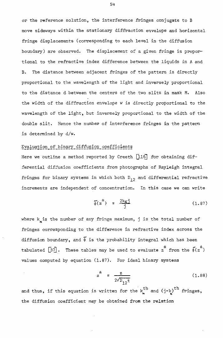
54

or the reference solution, the interference fringes conjugate to B

move sideways within the stationary diffraction envelope and horizontal

fringe displacements (corresponding to each level in the diffusion

boundary) are observed. The displacement of a given fringe is propor-

tional to the refractive index difference between the liquids in A and

B. The distance between adjacent fringes of the pattern is directly

proportional to the wavelength of the light and inversely proportional

to the distance d between the centers of the two slits in mask M. Also

the width of the diffraction envelope w is directly proportional to the

wavelength of the light, but inversely proportional to the width of the

double slit. Hence the number of interference fringes in the pattern

is determined by d/w.

Evaluation of binary diffusion coefficients

Here we outline a method reported by Creeth [ll^ for obtaining dif-

ferential diffusion coefficients from photographs of Rayleigh integral

fringes for binary systems in which both and differential refractive

increments are independent of concentration. In this case we can write

*(z") = (1.87)

where k is the number of any fringe maximum, j is the total number of Y\

fringes corresponding to the difference in refractive index across the

diffusion boundary, and (j) is the probability integral which has been

tabulated |_37j . These tables may be used to evaluate z from the <j)(z )

values computed by equation (1.87). For ideal binary systems

z = (1.88) 2/D-f

and thus, if this equation is written for the k^^ and (j-k)^^ fringes,

the diffusion coefficient may be obtained from the relation

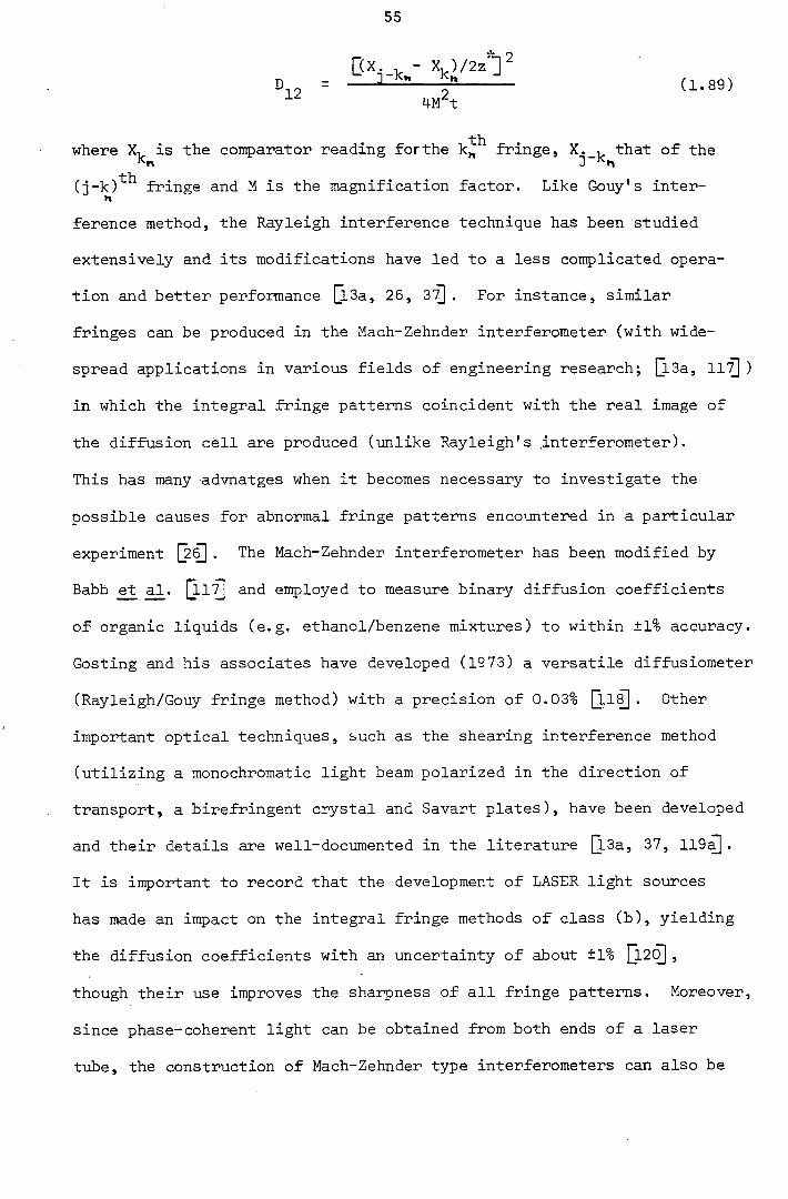
55

4M t

where X, is the comparator reading for the fringe, X._, that of the ] K-h

(j-k)"*" fringe and M is the magnification factor. Like Gouy's inter-

ference method, the Rayleigh interference technique has been studied

extensively and its modifications have led to a less complicated opera-

tion and better performance Q-Sa, 26, 3"^. For instance, similar

fringes can be produced in the Mach-Zehnder interferometer (with wide-

spread applications in various fields of engineering research; [l3a, 11'^ )

in which the integral fringe patterns coincident with the real image of

the diffusion cell are produced (unlike Rayleigh's interferometer).

This has many advnatges when it becomes necessary to investigate the

possible causes for abnormal fringe patterns encountered in a particular

experiment [2^ . The Mach-Zehnder interferometer has been modified by

Babb e_t al. [ll"^ and employed to measure binary diffusion coefficients

of organic liquids (e.g. ethanol/benzene mixtures) to within ±1% accuracy.

Costing and his associates have developed (1973) a versatile diffusiometer

(Rayleigh/Gouy fringe method) with a precision of 0.03% Q-l^. Other

important optical techniques, such as the shearing interference method

(utilizing a monochromatic light beam polarized in the direction of

transport, a birefringent crystal and Savart plates), have been developed

and their details are well-documented in the literature Q_3a, 37, 119^.

It is important to record that the development of LASER light sources

has made an impact on the integral fringe methods of class (b), yielding

the diffusion coefficients with an uncertainty of about ±1% [l2(^ ,

though their use improves the sharpness of all fringe patterns. Moreover,

since phase-coherent light can be obtained from both ends of a laser

tube, the construction of Mach-Zehnder type interferometers can also be

56

greatly simplified Q.21, 122]] . Perhaps the greatest achievement pro-

vided by laser sources has been the development of a relatively simple

and cheap technique namely that of holographic interferometry which,

unlike the previous methods, can be applied to very dilute solutions

[26, 12M-, 12^. In general, it must be realized that in order to enhance

the precision of the diffusivity measurements the resolution of the

optical method used must be increased and the influence of the concentra-

tion dependence decreased. This is the fundamental difficulty of the

limitation of the optical resolution [llCl •

1.4.2 Steady-State Diffusion - The Diaphragm-Cell Technique

The diaphragm-cell technique is one of the relatively simple and most

widely used methods for obtaining differential diffusion coefficients

for liquid systems of two and three components [37; Ch. 4, refs. 179-215].

First devised in 1928 by Northrop and Anson [l26j it was developed more

than twenty years later into a precision method, mainly by Stokes [l27,

12^, and it has proved particularly useful for the measurement of intra-

diffusion coefficients [l2^. All the experimental details of this

technique can easily be found in a number of publications [7, 13a, 127,

13C^ . In one of the simpler and more popular designs, a porous diaphragm

(glass, stainless steel or nylon) is used in a glass cell to separate

two solutions of different concentrations. Both solutions are mechanically

stirred so that, if the less dense (top) solution is separated from the

denser (bottom) solution by a horizontal diaphgram of essentially constant

thickness, then all concentration gradients are in the diaphragm. Hence

if it is assumed that the diaphragm is in a steady-state, then there

would be no accumulation of material in the diaphragm during the time

that transport by diffusion is taking place. Thus at a particular time

the flux of each component across any plane parallel to the horizontal

57

direction is independent of diaphragm thickness £, But due to the solute

conservation in the cell, each is time-dependent so that in the

following treatment for obtaining the differential diffusion coefficients,

based essentially on the works of Barnes [iSjTj, Gordon [l3:^ and Stokes

[l2'f], it is convenient to write J^(t).

Let the positive direction of z coordinate be in upward direction and

consider the changes in solute concentration taking place in the bottom

and top cell compartments of volume Vg and V^, respectively. In the

bottom compartment

dC = -J(t) (1.90)

B

and in the top compartment

dC ^ W = (1.91)

where Cg and are the solute concentrations in the bottom and top

compartments and Ap is the effective cross-section of the pores in the

diaphragm. Combining these two relations and denoting (Cg-Crj,) by AC

we obtain

^ ^ (1.92)

It is convenient to define the average value of the differential diffusion

coefficient over the concentration range Cg to C,p by the time-

dependent integral diffusion coefficient, D(t), using equation (1.13)

C_ , I ^ If = - A / D^^(|i)dz = M M (1,93)

Z—u

Thus, combining this equation with (1.92)

• ^ 4 ^ = -- (1-94)

where 3^ (typically 0.07 - 0.2; [l3^) is the cell constant. Integrating

58

this equation over the experimental duration t yields

Ac" t _ in = 8 / D(t)dt (1.95)

AC c Q

and _ 1 AC*' D = ^ ^ (1.96)

I f Acf-

where D = (L/t)/^ D(t)dt is the time average of the diffusion coefficient

D(t) and AC° and AC^ are the initial and final concentration differences

of the solute, each for the top and bottom compartments. For the special

case that the diffusion coefficient is independent of concentration,

equation (1.96) obviously gives the differential diffusion coefficient

directly. If and D t f(C), then D is the differential diffusion

coefficient at the average concentration of the two compartments. Equation

(1.96) may also be used to obtain intradiffusion coefficients, when com-

position of the system is essentially identical in both sides of the

diaphragm cell. If, however, D = f(C), Gordon |j.3^ has shown that (to

approximately 0.02%)

"c , D = — D dC (1.97)

AC 12

where , . + _ c; + gt ___ _ _

Cg = = -i-2—- and AC = Cg - (1.98)

In order to compute differential diffusion coefficients at particular

concentrations from the integral values, an analytical expression with

arbitrary coefficients is usually assumed for ~ f(C)], and these

coefficients determined from the measured values of D, Cg and C^ by,

for example, a least-squares procedure.

Since the development of the diaphragm cell by Stokes, many changes have

been proposed in the materials used for the diaphragm [128, 134, 13^ in

the cell geometry [39, 135-13^ and stirring method [j9, 133], and in the

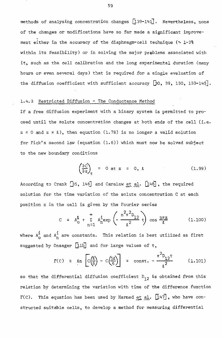
59

methods of analysing concentration changes [l39-m-lj. Nevertheless, none

of the changes or modifications have so far made a significant improve-

ment either in the accuracy of the diaphragm-cell technique 1-2%

within its feasibility) or in solving the major problems associated with

it, such as the cell calibration and the long experimental duration (many

hours or even several days) that is required for a single evaluation of

the diffusion coefficient with sufficient accuracy (3o, 39, 130, 133-145].

1.4.3 Restricted Diffusion - The Conductance Method

If a free diffusion experiment with a binary system is permitted to pro-

ceed until the solute concentration changes at both ends of the cell (i.e.

z = 0 and z = £), then equation (1.78) is no longer a valid solution

for Pick's second law (equation (1.6)) which must now be solved subject

to the new boundary conditions

(fi) = 0 at z = 0, & (1.99)

According to Crank [35, 14^ and Carslaw _et a2. [l4^ , the required

solution for the time variation of the solute concentration C at each

position z in the cell is given by the Fourier series

/ n TT D \ C = A* + Z A^exp ( tj cos (1.100)

n=l \ / *

where A^ and A^ are constants. This relation is best utilized as first o n

suggested by Onsager [lib] and for large values of t,

F(C) 5 &n - <f const. — (1.101) Z

so that the differential diffusion coefficient is obtained from this

relation by determining the variation with time of the difference function

F(C). This equation has been used by Hamed et [l47] , who have con-

structed suitable cells, to develop a method for measuring differential

60

diffusion coefficients for dilute binary electrolyte solutions [l3a, 3"^ .

At large values of t the function F(C) was found to be directly propor-

tional to the same function of the reciprocal resistance of the electrolyte

solution. Thus determination of the absolute values of the electrolyte

concentrations were unnecessary. Using the literature data, it was

verified that for dilute KCS, solutions negligible error is introduced

by assuming the difference in concentration to be proportional to the

difference in reciprocal resistance, a relationship which subsequently

has been applied to many other systems. Hence in this method, the

reciprocal resistances at the two fixed positions in the cell are deter-

mined as a function of time (= F(C) as f(t)), and the diffusion coef-

ficient is obtained as previously described. An experiment may take over

a week to yield a single diffusion coefficient with a precision of about

0.3%.

1.4-.4 Taylor Dispersion Technique

This is a flow method ideally based on the study of the dispersion of

a delta function pillse of a solution, injected at time zero into a stream

of liquid flowing in a laminar regime through a long straight tube with

a uniform circular cross-section. The technique is also referred to as

the "chromatographic method" and has been described in detail elsewhere

(Chapter 2 and |j.8, 21, 23, 24] ).

In 1953, Taylor [l4^ first showed that the injected pulse is dispersed

(as observed initially by Griffiths in 1911; [24]) by the combined

action of the laminar velocity profile and molecular diffusion (essen-

tially in radial direction). Hence after an initial transient period

(t^) the injected material is distributed normally about an origin moving

at the mean velocity (U^) of the stream. Physically, the reasoning can

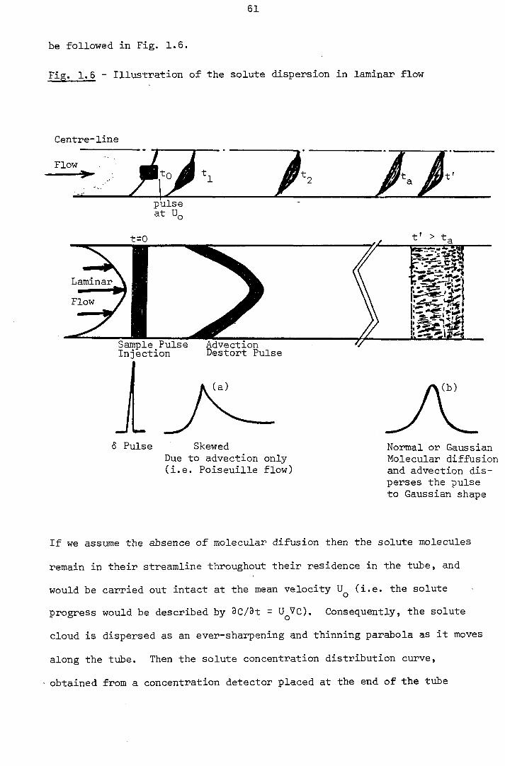
61

be followed in Fig. 1.6.

Fig. 1.6 - Illustration of the solute dispersion in laminar flow

Centre-line

Flow a pulse at

t=0

Laminar

Flow

Sample Pulse Advection Injection Destort Pulse

t' > t-a m

(a)

6 Pulse Skewed Due to advection only (i.e. Poiseuille flow)

(b)

Normal or Gaussian Molecular diffusion and advection dis-perses the pulse to Gaussian shape

If we assume the absence of molecular difusion then the solute molecules

remain in their streamline throughout their residence in the tube, and

would be carried out intact at the mean velocity (i.e. the solute

progress would be described by 3C/3t = U^VC). Consequently, the solute

cloud is dispersed as an ever-sharpening and thinning parabola as it moves

along the tube. Then the solute concentration distribution curve,

obtained from a concentration detector placed at the end of the tube

62

(Chapters 2 and 3), will be highly skewed as shown by Fig. 1.6(a).

However, this assumption of no molecular diffusivity is far from reality

in liquids and cannot be verified experimentally. The experimentally

observed shape of the curve is almost Gaussian as shown by Fig. 1.6(b).

This is because the solute molecules at the tip of the parabola (i.e.

at the centre line) diffuse towards the tube wall into a streamline of

lower velocity, while those near the wall (parabola tail) diffuse towards

the centre line into a higher streamline velocity. This phenomenon

minimizes the stretching of the parabola through a recirculating motion

of the solute cloud, as if stirred by a molecular stirrer, with a speed

that depends on the molecular difusivity, flow rate and tube diameter.

If the cross-section averaged concentration of the injected material is

observed as a function of time at some distance (L) downstream from the

point of injection, the moelcular diffusion coefficient can be obtained

from the moments of the eluted solute distribution (see Chapter 2 and

[l8, 21, 23, 2 ^ for binary-, self-, and intra-diffusion coefficient

measurements). It is important to note that the theoretical analysis of

the dispersion process given originally by Taylor , and later more

exactly by Aris [l4^, was not intended to form the foundation of a

technique for diffusivity measurements, but rather to predict solute

dispersion in pipelines. Consequently, the use of this theoretical

description of the dispersion process without modification for the par-

ticular application of diffusivity measurements has, in the past, been

justified on.the basis of empirical observations. Such procedures

inevitably degrade the accuracy of the experimental data obtained, and

for this reason: the method has been termed one of moderate accuracy

[2^. In Chapter 2 we provide a more complete treatment of the theory

of the Taylor dispersion technique for diffusivity measurements in order

63

to obtain a set of working equations for an instrument operating on this

principle. In turn, these equations permit us to assess the accuracy of

the results of measurements with this method, and to show that it can

be made comparable with that of other techniques. Measurements of the

binary diffusion coefficients reported in Chapter 4 support this con-

tention.

Most of the reliable diffusivity data for liquids have been obtained

through the use of highly sophisticated but relatively expensive and

painfully slow experimental techniques, usually involving the use of free

or porous diaphragm diffusion cells. One of the difficulties encountered

in a free diffusion technique is in establishing an initially sharp

boundary between the pure solvent and the solution. Maintaining an

undisturbed medium (minimizing vibration) throughout the experiment has

also been a major problem. Although the porous diaphragm diffusion cell

method minimizes most of the problems that arise in a free diffusion

method, it has some drawbacks of its own. Since it requires a porous

membrane, with some resistance to the transport of the solute, the

technique does not yield diffusion coefficients directly and needs to

be calibrated with a known standard. Other problems related to the use

of the porous diaphragm such as adsorption of solute on the surface of

the porous membrane, bulk streaming and semi-permeability due to

improper selection of diaphragm porosity can also occur. The method

cannot easily be employed as a continuous observation type and requires

a relatively long period of time (two or more days) to complete a single

diffusion measurement. All of these problems are reduced if diffusion

experiments are conducted by the Taylor dispersion technique.

In addition to being relatively fast (a few hours at the most to complete

the measurement), the Taylor dispersion technique requires only microgram

64

sized samples instead of the gram amounts needed by the free or steady-

state diffusion methods. It is also versatile (gaseous/liquid mixtures;

[23, 27, 2 ^ ) and easily adaptable to extremes of temperature and pressure

(high pressure increases solubility which in turn makes the detection

of the dispersion peak easier). Nevertheless, it is true that measure-

ments with the highest precision are obtained by optical methods, but

they cannot be employed over a wide temperature range because it is only

near room temperature that sufficient temperature stability and uniformity

can be maintained. Thus the Taylor dispersion method represents a reason-

able compromise between the precision and the extent of the temperature

range which can be investigated for a system.

When the technique is fully refined (see Chapters 2 and 3) it enables the

measurement of diffusion coefficients with an accuracy of ±1%. It is

an absolute method and hence does not involve the uncertainties associated

with calibration using systems of known diffusivity, which is inherent

in the porous disc (or frit [l5l]) and diaphragm cell methods .

Furthermore, when the technique is applied to gas/liquid mixtures it

does not require precise solubility data as is the case in absorption

methods Q , ^ and accurate chemical analysis of the liquid phase is

unnecessary.

1.4.5 Other Important Methods

The methods described above are the only ones which have yielded a large

body of data over a wide range of conditions with high precision. There

are a number of methods which have been employed with some success to par-

ticular types of liquid systems such as polymers in liquids. However,

for mixtures of simple liquids used techniques have not yet been developed

to the point where accurate measurements can be made. Such techniques

include the n.m.r. Spin-Echo (observing the effect of diffusion on the

65

decay of n.m.r. signals; precision ~2-5%) and the Light Scattering

methods ("light-beating spectroscopy"-,central to photon correlation

spectroscopy, or "line broadening" - precision ~l-4%) which have been

described in the literature (^4, 26, 152, 15^.

65

C H A P T E R

THE THEORY OF THE EXPERIMENTAL METHOD

2. 'Introduction

The need for accurate measurements of the transport properties of fluids

and, in particular, the diffusion coefficient in mixtures was emphasized

in the introduction of this thesis. As has been indicated, and illust-

rated in Chapter 1, the lack of accurate experimental data for diffusion

coefficients in liquids,arises from a combination of the inherent slow-

ness of the diffusion process and the failure to develop reliable theories

of some techniques for their measurement [7-9,11,18-20,30]. The Taylor

dispersion technique [ch. 1, Section 1.4.4] employed for the measurements desc

ribed in this thesis offers the opportunity for rapid diffusion coeffi-

cient measurements which may also be made accurately, provided a suitable

theory of the method is available. The present chapter is dedicated to

providing this theory in the form of a set of working equations combined

with a full set of corrections.

2.1 The Principle of the Experimental Method

We consider first the simplest mathematical model of an instrument to

measure liquid phase diffusivities using Taylor dispersion. This mathe-

matical model refers to an idealized experiment, which cannot be

realized in practice. Nevertheless, it will be-shown that a practical

instrument can be designed such that its departures from the ideal are

small and so that they may be evaluated with the aid of a proper analysis,

Figure 2.1 shows the ideal experimental arrangement and defines the

geometry of the.apparatus. For generality, we consider a homogeneous

liquid mixture of species 1 and 2 flowing in laminar flow through an

67

infinitely long, isothermal, straight tube of uniform, circular cross-

section, radius R^, with impermeable walls. We denote the molar concent-

rations of the species in the flowing mixture by and respectively.

The mean velocity of the liquid mixture in the tube is denoted by U^.

At time t = 0, a sample of liquid mixture of the same two components but

of a different composition is introduced into the tube by injection as

a "5 pulse" at z = 0.

Fig. 2.1 - The ideal Taylor dispersion experiment 6 pulse dispersed by the combined effects of the laminar velocity profile and molecular diffusion —

t.o t.t

" 4-

g -PulsA input GiaussCan owctpwt

fkrctijolit 2=0

The molar concentrations of the two components in the sample are

and respectively and its mass density is supposed to be the same as

that of the flowing stream. The sample fills the cross-section of the

tube at z = 0 completely, it is of uniform composition over this cross-

section and is supposed to extend infinitesimally in the axial direction.

Therefore the only perturbation of the flowing stream arises from the

change in the concentration of component 1 at z - 0 which may be represen-

ted by a delta-function, 6(z), which is normalized so that

68

ttR^ f 6(z)lc^^ - Cjdz = (2.1)

where 6(z) = 0 for z ^ 0, and represents the number of moles of

component 1 in excess of those present in the same volume of the flowing

stream.

The concentration gradient established by the introduction of this sample,

together with the action of the parabolic velocity profile of laminar

flow results in dispersion of the pulse. The process of molecular dif-

fusion involved is clearly that of mutual or interdiffusion and, in the

present analysis, the appropriate diffusion coefficient, is sup-

posed to be independent of the composition of the liquid mixture.

If we denote the perturbation to the flowing stream composition caused

by the pulse by AC^(r, 6, z, t), then the differential equation for AC^,

describing the dispersion, is

5 1 - 2 ( ^ ) o

9(AC^) ,

3z ( 2 . 2 )

and the conditions for its solutions are, at t = 0,

AC^(r, 6, 0, 0) = 6(z)(C^i - C^^) , (2. 3)

6(z) 0 for z = 0

and 9(AC^)

= 0 at r R for all t o (2.4)

together with sufficient conditions on AC ^ for z = ±<».

In his original analysis, Taylor [l4^ introduced an approximation con-

cerning the relative magnitudes of axial and radial dispersion so as to

render the solution of equation (2.2) practicable. But in this work we

prefer to follow the analysis of Aris [iM-G f, and to seek solutions for

various spatial moments of the concentration distribution, since these

turn out to be sufficient for the analysis of the experiment.

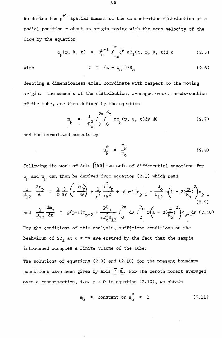
69

We define the spatial moment of the concentration distribution at a

radial position r about an origin moving with the mean velocity of the

flow by the equation

00

c (r, 0, t) = f AC^(C, r, 0, t)d C (2.5)

with G = (z - U^t)/R^ (2.6)

denoting a dimensionless axial coordinate with respect to the moving

origin. The moments of the distribution, averaged over a cross-section

of the tube, are then defined by the equation

2-n ^o m^ = —^ f f rc (r, 0, t)dr d0 (2.7) P . nR 0 0 P

o

and the normalized moments by

A % "p = (2-8)

Following the work of Aris [iM- two sets of differential equations for

c and m can then be derived from equation (2.1) which read p p

9c , . / 3c\ , 9^c U , 2\

^ ; 3? - a f ) + + P ' P - D V 2 " ^ " ' ' f y p - i

(2.9) dm pU 2tt Rq / 2\

and = p(p-l)m 2 + — o / d0 / r(l - 2(-^) p fir (2.10) 12 ^ P trR D 0 0 \ o / ^

For the conditions of this analysis, sufficient conditions on the

beahviour of AC^ at ? = i"*" are ensured by the fact that the sample

introduced occupies a finite volume of the tube.

The solutions of equations (2.9) and (2.10) for the present boundary

conditions have been given by Aris jl4^. For the zeroth moment averaged

over a cross-section, i.e. p = 0 in equation (2.10), we obtain

A m^ = constant or = 1 (2.11)

70

which merely states that the total quantity of the injection sample is

constant. Furthermore,

= 0 = (2.12)

which expresses the fact that the mean of the distribution, averaged over

a cross-section, travels in the tube with the mean velocity of the flow.

The solution of equation (2.9) for period 2ir in 0 and with the boundary

conditions

(2.13) Cp(r, e , 0) = Cpo(r, 0)

9c

^ = 0 at r = (2.14)

gives the mean of the distribution, as a function of radial position in

the tube as

- R : -

(2.15)

th with representing the n zero of dJg(z)/d^, where is the zeroth-

order Bessel function of the first kind. It is useful to record that the

original expressions for c^ and given by Aris were found to be incor-

rect in the sign as indicated by Tillman [l4-9''i]

The cross-section averaaged second moment, may also be derived, and

is given by the expression

o o 12 48D

12

/ R V \ <» t - 128 ( ) E a

D 12 /n=l on

1 - exp " ^ 1

R^ (2.16)

O / _J

It has been shown by Aris that the longitudinal distribution of concent-

ration approaches that of a normal distribution as t The expression

for the skewness of the cross-section averaged distribution is

(%t)' Sk = (2.17)

(Wg)

71

which is given asyn^totically by the relation

i+9U R®

" ^ . - 4 : -m v . 4 8 D 1 2 /

indicating that the approach to normality occurs as t

Equations (2.12) and (2.16) yield the fundamental working equations for

the analysis of the ideal experiment. It is clear that the exponential tran-

sient term in equation (2.16) can be made to decay arbitrarily rapidly

by the choice of suitable conditions. Thus for

°12 t > 0.6 (2.19)

R o

the transient term contributes less than 0.01% to the second term of

equation (2.16). Hence if condition (2.19) is satisfied, equation (2.16)

may be written as

R^U^X 128 R^U^ ^2 = 2(Dl2 + t - --^2-2-°

(3.8317)® (7.0156)® (2.20)

Because the mean velocity of the flow can be chosen independently of the

time tj we note that if

"o ^ (2.21)

then equation (2.20) reduces to the form

with an associated error of less than 0.01% which we regard as negligible.

In this equation, we have written

00 K = E a"® = 2.1701 ... x 10~^ (2.23) = n=2

for convenience. Condition (2.21) is easily satisfied for measurements

in liquids while maintaining the fluid flow in the laminar regime.

t > 700

72

Equation (2.22) could evidently form the fundamental working equation

for the ideal experiment, since the binary diffusion coefficient 0^2

could be derived from experimental measurements of the second moment,

with the aid of it. For later use, it is more convenient to employ

a limiting form of this equation. Since the duration, t, of the measure-

ment may be chosen arbitrarily, the time-independent term in equation

(2.22) may be made negligible (less than 0.01%) by choosing

(2.24)

This selection automatically ensures that the transient term in equation

(2.15) is even smaller than that corresponding to condition (2.19). In

this case, equation (2.22) reduces to the very simple form

where the subcript s implies that conditions (2.21) and (2.24) are

satisfied in the experiment. Furthermore, by virtue of equation (2.12),

the fluid mean velocity may be determined from the first moment of

the distribution with respect to the fixed origin z = 0., Denoting the

first moment by z, it follows that

U = % (2.26) O "t

so that the final working equation for the ideal diffusion experiment becomes

= - 4 r - (2.27)

Hence a diffusion coefficient determination may be performed by measuring

just the first and second spatial moments of the cross-section averaged

concentration distribution of the injected sample, after flowing for a

time t through a tube of known radius.

73

If condition (2.24) is not satisfied, the second moment required in

A '2 = equation (2.27) can still be derived from the measured moment, by

application of the correction in the form

A * & ^2s = ^2 + " 2 (2.28)

where

Provided that

u. 2 128KR

6y" = (2.29) °12

t > 20 (2.30)

A the correction amounts to no more than 0.3% (0.06% under selected

sV

conditions for the measurements of this work) of so may be

calculated with sufficient accuracy using an estimate for

Finally, in this section, we record for future use that if conditions

(2.21) and (2.22) are satisfied, then the absolute skewness of the spatial

• • ~ 8 •

distribution is less than 5 x 10 , so that for all practical purposes

the distribution may be regarded as normal. Furthermore, it follows

that the Taylor dispersion process under the conditions specified may

be equally well-described by the one-dimensional differential equation

[148, 14^.

where E is an effective diffusivity given by

and is the concentration perturbation averaged over a cross-section.

This one-dimensional representation is equivalent to the process of

plug flow plus axial diffusion with a diffusivity E. The moments of

the solution of equation (2.31) are identical to those for the solution

of the full diffusion equation under the above conditions.

74

2.2 Practical Considerations

The ideal experimental method outlined in the previous section is not

practicable for measurements of diffusion coefficients. Furthermore,

even if it were, it would not be possible to construct an apparatus

which excactly conforms with the ideal. In order to perform such

measurements using the same principle, it is therefore necessary to

make changes to the experimental method and to examine the ways in which

a practical instrument departs from the ideal. Such departures may be

classified under four headings:

1. Concentration Distribution Determination.

2. Sample Introduction.

3. Diffusion Tube Geometry.

4. Concentration Dependent Fluid Properties.

We shall examine each of these in turn in the following sections and,

where it is appropriate, express the effect of the.departure from the

ideal instrument as a small correction to the ideal working equations.

In some cases, it will be possible to render the corrections negligible

by proper design. In other cases, the correction can only be made

small by design, but then it can be estimated with sufficient accuracy

to make the contribution to the overall uncertainty in the diffusion

coefficient measurements negligible.

In the following sections of this chapter, we examine the consequences

of the above considerations for the design of an apparatus and the working

equations for the analysis of the experimental data. In this examina-

tion, we shall presume that all the corrections due to the non-ideal

model are small, so that they may all be treated as first-order pertur-

bations. In this case, we may further assume that the interaction bet-

ween any two or more of these first-order effects is negligible so that

75

each perturbation can be treated independ.ently. The conditions under

which such assumptions are valid will, of course, emerge from the

analysis and form the basis of the design criteria.'

2.3 Concentration Distribution Determination

2.3.1 Temporal moments

It is much more convenient experimentally to observe the concentration

distribution at a particular cross-section in the tube as a function

of time, rather than to observe it at one instant of time as a function

of axial position. Therefore we consider the diffusion process des-

cribed earlier in the ideal apparatus again, but now we suppose that

we can determine the cross-section averaged perturbation of the concen-

tration of component 1, denoted by AC^^, at an axial position z = L, in

an infinitesimally small length of the diffusion tube. Then, in order

to relate the temporal moments of the distribution observed in this way

to the spatial moments of the previous section, we use the result

derived there that the spatial distribution is essentially normal.

For such distribution we can write [14^

N, AC exp

(z-Ugt)' — —

L_ _J

(2.33)

For an observation carried out in the cross-section at the axial position

z = L, we define

A

and ; = 2U Lt o

Equation (2.33) can then be rewritten as

AC Im

N _ i — (w s T) 5 exp

2mR^L o

(1-T)'

4 C T (2.34)

76

The normalized temporal moments of this distribution, for a measurement

carried out in the idealized apparatus, are then defined by

the equation T P T.

( A , ; TP dT

= 53 ( 2. 35)

; ACim dT 0

In general, the quantity C is time-dependent, due to the definition of

A

^2 in equation (2.22), and the analytic evaluation of equation (2.35)

is impossible. Consequently, we seek approximate solutions for the

temporal moments. Because the time-dependent part of t, is generally

small (less than 0.6% if condition (2.30) is satisfied), these approxi-

mations will prove sufficiently accurate.

2.3.2 Zeroth-order approximation

If both conditions (2.21) and (2.22) are satisfied, then with negligible

error,

y" RV ^ ~ ^o " 2U Lt ~ 48LD (2.3,6)

O _Lz

which is time-independent. The evaluation of the first raw temporal

moment, leads to the result of Pratt and Wakeham [2^

tid = IT ^ (2-37) o

/ ,

Under the same conditions, the second raw temporal moment,- (y2^id'

been evaluated by Levenspiel and Smith [jssj as

2 S ' i d = rT r " ) (2-38)

2 so that the temporal variance of the distribution, denoted by may

be written

" Ij^l^i^ = (rr) + 25^) (2.39a)

77

'"8? + 2C o o

(2.39b)

Here the subscript (id) denotes that the various moments refer to measure-

ments in the ideal diffusion apparatus of the previous section. Equation

(2.39) can be solved exactly for to yield

2a id-tid+ (2.40)

Finally, from equations (2.37) and (2.25), we note that

/ 1 °12

48tid

so that using equation (2.40) in (2.41), we obtain the final working

equation for the experiment in the form

(2.41)

R D 12

2^^id

1 + -LT ^id

+ 3

(2.42) o I o -

With this equation the diffusion coefficient can be determined from

measurements of the first two temporal moments of the concentration dis-

tribution at a particular cross-section of the tube.

2.3.3 First-order approximation

If condition (2.21) is satisfied, but the measurement time, t, is such

that'condition (2.24) is not satisfied, it is still possible to obtain

an analytic working equation provided that condition (2.30) on the dif-

fusion time is met. In this case we can write

where 5; =

•6tKR'*U c o o

78

The major contribution to the integrals in equation (2.35) arises from

near t = 1. Thus we may employ a quasi-steady state approximation to

evaluate the small correction 6?, i.e. we evaluate 6^ at t = , o

6; = -

4 2 64KR U

c o o

and so 6? within this approximation can be treated as time-independent.

If now the procedures of the zeroth-order analysis are carried through

again, using in place of the final working equation becomes

12

R^ 1 o ) ['•«

2

+ 3

24tid ] + &(1 - 6 J (2.43)

where

5 = (768) KC a CO

Again, the working equation relates the diffusion coefficient to the first

two temporal moments of the distribution observed in the diffusion tube.

Provided that condition (2.30) is satisfied, the term 5^ contributes at

most 0.6% to the measured diffusion coefficient, so that the foregoing

analysis for its estimation is sufficiently accurate. Hence equation

(2.43) constitutes the fundamental working equation for the evaluation of

diffusion coefficients from temporal moment measurements in this work.

Finally, we note that if D^gt/Rg ) 20, (c.f. ^ 50/(3.8)^ an

empirical result obtained by Pratt and Wakeham [l^ in order to satisfy

Taylor/Aris criterion), so that condition (2.30) is satisfied, then

^ 10 o

-3 (2.44)

and hence from equations (2.25) and (2.38) we can write (with an error

of no more than 0.2%)

79

So = (2-45)

This equation and condition (2.44) will only be used as a design criterion

-3

and constraint later on. For the condition < 10 , equations (2.39)

and (2.4-1) may be linearized with respect to as it has been done by

other workers^2sj- In this case, the approximate working equation (with

an error of less than 1%) which is found useful later, becomes

D,. = . (2.46)

2.3.4 The concentration monitor

The preceding analysis were based upon the assumption that the average

concentration in a cross-section of the diffusion tube could be deter-

mined at a particular axial position. In practice, such a measurement

is not possible and some average concentration in a finite length of the

tube must be determiend instead. There are two ways in which this may

be accomplished, both of them being considered in the following sections.

2.3.5 A section of the diffusion tube

Figure 2.2 represents a schematic diagram of the concentration monitor

as a section of the diffusion tube. In this concentration monitor, we

assume that it is possible to determine the average perturbation to the

concentration of the flowing stream in a small length 6L of the .tube

itself, beginning at z = L. We denote this average concentration pertur-

bation by AC^, defined by the equation

L+6L R 2ir AC, (L, t) = — 5 — / / ° / AC^(r, 6, z, t)d8 r dr dz (2.47)

ttR SL L 0 0 o

A composition monitor of this type can be used when one of the components

of the perturbing pulse is radioactive [28,15oJ. The detector would then

consist of a test section of the diffusion tube within the field of view

of a suitable activity monitor which would define the length 6L observed.

80

Fig. 2.2 - The concentration monitor as a finite length of the"diffusion tube

This might be employed for measurements of self-diffusion coefficients

of liquids. Clearly, because of the non-zero volume of the detector

the temporal moments of AC^ will not be identical to those of

Introducing again the cross-section averaged composition perturbation

AC^^, equation (2.47) can be written in the form

L+6L AC^ (L, t)

6L / AC. dz

Im

Assuming that all of our previous conditions are satisfied in the

experiment, then we can use equation (2.33) for AC^^ so that AC^(L, t)

becomes

N,

'"1 ~ 3 sV 1 2

L+6L f exp

(z-Ugt)

2u 2s

dz (2.48)

setting y!!! = yZ for the present purposes. Evaluating the integral in '2 " 23

equation (2.48), we obtain

N AC,

2itR 6L o

erf (1-T) ^ SL/L

(4; t)2 (4; T)2 l_ o o _1

erf (1-T)

J ' + V J

(2.49)

with T and being defined earlier in Section 2.3.1.

According to the approach outlined earlier in Section 2.2, we can now

suppose that 6L/L is small; in particular that

81

<< T)* L o

In this case the error function in equation (2.49) may be expanded by

a Taylor series in the form

N, AC^CL, t) =

2TTR L o

— (n^gT) ^exp (1-T)' 4; T

l_ o _J

1 _ ilcll (SL) + L 3(4C^T)

2(1-t)^ (1+C x) - 1 ( , .... (2.50)

This result allows the computation of the normalized temporal moments

of the distribution AC^(L, t), defined in the standard manner. After some

laborious algebra, it can be shown that the first moment is given by

- = i (1 . . % ) = I = t,, . i ( ^ )

o o (2,51)

and the variance by

5L, 1 o' L' 12' L

(2.52)

correct to the order of ( ~ ) • We use suffix (expt) to denote the

measured or experimental moments.

Comparison of equations (2.51) and (2.52) with those for the ideal

moments, equations (2.37) and (2.39), reveals the form of a correction

to be applied to each measured moment to recover the ideal moments.

Thus

and

Here

t.j = t . - 5t id expt o

0?, = - 6a^ id expt o

6t, 6L 2U

(2.53)

(2.54)

(2.55)

and r- R 6a = 6L

o + 6L

48D12U0 120= o

(2.56)

82

Therefore both corrections may be calculated from a knowledge of the

mean velocity of the flow and an estimate of the diffusion coefficient.

For the purpose of design, we may assume that = L/t^^ and ) 20

-3 (i.e. X, ^ 10 ). With these approximations we find

^ «L

^ 6L 2 " L

°id

J + 40 xJ so that for 6L/L ^ 0.01, the corrections to either moment become 30.9%

indicating that the method proposed for their estimation must be satis-

factory.

2.3.6 A small volume at the tube exit

The most commonly used concentration monitor consists of a small sampling

volume V^, placed at the exit of the diffusion tube. The concentration

of the effluent from the tube in this volume is usually measured with a

refractive index detector [l^,19,23,27,30] an instrument which has been

employed in the measurements reported in this thesis. The differences

between the moments observed with this type of detector and the ideal

ones are difficult to -analyse because the flow pattern and geometry of

the sample volume are not well known. Consequently, we examine two

extreme cases to set bounds on the effect and to provide guidance for

the design of an instrument.

First we consider that within the sample volume the dispersion process

proceeds unaltered and that the refractive index detector determines

the average concentration of the dispersing material within it. In

this case, the analysis is identical to that given above, and, in terms

of the detector volume, the corrections to the moments are

83

and 6a la

U I 2 o V 2ITR L

Q

TTR L

(2.57)

(2.58)

An alternative model of the detector is one that behaves as a perfectly

mixed volume in which the composition is uniform. This model, which is

probably closer to reality, is illustrated schematically in Fig. 2.3

below.

Fig. 2.3 - The concentration monitor as a perfectly mixed volume, V^, at the exit of the diffusion tube

oLctftctdr wfume

bWfosufttj E

Plwgtww

Per-ftcty tnixtd region

ac a

4 A

The presence of the perfectly mixed region implies that there exists now

a boundary condition for the diffusion equation at the exit from the

diffusion tube, and not at infinity, as described previously.

In order to analyse this problem, we first make use of the result given

earlier. That is the description of Taylor's dispersion process, for the

present condition j_2 ' o > means of the one-dimensional diffusion

equation (2.31) to a very good approximation. For the model of the dif-

fusion tube and detector shown in Fig. 2.3 above, the boundary conditions

for the solution of this equation are:

at z = 0

and at z = L

^^im " C^^) (2.59)

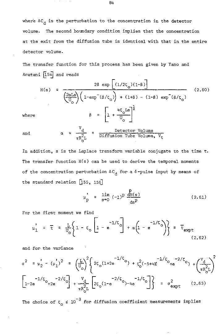
84

where AC^ is the perturbation to the concentration in the detector

volume. The second boundary condition implies that the concentration

at the exit from the diffusion tube is identical with that in the entire

detector volume.

The transfer function for this process has been given by Yano and

Aratani {l5^ and reads

26 exp [(1/2^^)(1-B)] H(s) =

/2aLs\ l-exp + (1+B) - (1-3) exp (6/?^)

(2.60)

where

and

8 = 1 + U

a = Detector Volume ^^2^ Diffusion Tube Volume, V^

o

In addition, s is the Laplace transform variable conjugate to the time t.

The transfer function H(s) can be used to derive the temporal moments

of the concentration perturbation AC^ for a 6-pulse input by means of

the standard relation [l55, 15^

Vi p s-»-0

For the first moment we find

L

' _ lim ^_^jp dH(s) (2.61) ds^

^1 = t = 1 - So -1/C.

1 - e -1/5.

+ a 1 - e = t expt

( 2 . 6 2 )

and for the variance

2 ' , \2

t -

-1/G_ -2/G

2e +2e

-3

-2/c -1/C (1-e °)-4e ° O ^ (2.53)

expt

The choice of $ 10 for diffusion coefficient measurements implies

85

that the exponential terms in equations (2.62) and (2.63) are entirely

negligible, and we obtain sinply

'expt L U 1 - So + 2

irR L_ o

r V = tid + U"

o #: - (2.64)

and

expt TTR L TTR L

irR L

TTR L " o

= tid + (U

(2.65)

The corrections to be applied to the experimental moments observed with

this detector in order to recover those of the ideal experiment can then

be obtained by comparison with equations (2.37) and (2.39a). That is,

and

where

'id

" L

" texpt -

= °expt - ' " L

and 6a lb

o V TTR L

t tR L

( 2 . 6 6 )

(2.67)

In both of these corrections, the last terms arise from the modifications

of the diffusion process caused by the perfectly mixed region, whereas

the remaining terms are due to the non-zero volume of the detector. These

latter terms are naturally somewhat larger than those for an unmixed

detector of the same volume given in equations (2.57) and (2.58). In a

practical instrument, if it is known which type of model detector repre-

sents the reality most closely, then the appropriate corrections given

above should be applied. However, it is most likely that a practical

detector will have a behaviour intermediate between these two extremes.

86

Therefore, it is best to design the instrument so that the corrections

evaluated for either model are negligible. Irrespective of the possible

external constraints dictating the detector volume V^, the relative

errors due to all the corrections can be made arbitrarily small by the

selection of the length of the diffusion tube, L, for a fixed fluid

velocity and diffusivity.

2. Sample Introduction

So far, we have been concerned with the evaluation of the temporal

moments of the concentration distribution based upon a delta function

injection of a sample at z = 0, which is uniform across the diffusion

tube cross-section. In this section, we recognize that it is impossible

to provide such a 6-function pulse in practice, and suggest an alter-

native. It is relatively straightforward to introduce an approximately

rectangular pulse of a sample into the tube at z = 0, which is uniform

across the diffusion tube cross-section.

Therefore, we now consider the temporal moments of the concentration

distribution detected in a cross-section at an axial distance z = L, as

a result of an exactly rectangular pulse input. For this input, the

original boundary conditions of equation (2.3) at z = 0 is modified to read

AC^(r, e, 0, t) = (C^^ - 0 < t ( ±1

AC^(r, 9, 0, t) = 0 otherwise (2.68)

2

The injection time t ^ is equal to V /TTR^U , where is the volume of

the sample injected. Instead of solving the complete Taylor dispersion

problem subject to this new boundary condition, it is much simpler to

use the approximation that the dispersion process can be described by

the one-dimensional equation (2.31) as the effect of rectangular pulse

87

injection is expected to be small. In this case, the problem is a

standard one and its solution is obtained by the transfer function method

described in Section 2.3.6. The results for the first raw moment and

the variance observed at a fixed cross-section in the tube are Q.54]

'expt tr o

and

expt

2TrR L

(2.69)

(2.70)

+ 8(2 + J .

TTR L

2 - 1

Thus

with TTR L

TTR L

(2.71)

(2.72)

As for the non-zero volume of the detector, the corrections are made

smaller by increasing the diffusion tube volume for a fixed injection

volume. Provided that the corrections can be made sufficiently small,

departures from a true rectangular pulse will have an insignificant

effect upon the observed moments.

2.5 Diffusion Tube Geometry

The analysis of the ideal experiment presumes that the diffusion tube

is straight, and of uniform, circular cross-section. We have already

88

established in Sections 2.3.4 and 2.4 that in order to minimise the

corrections arising from the concentration distribution and sample

introduction, the tube must be as long as possible for a fixed mean

velocity of the flow. Since there is a practical lower limit to the

flow velocity that can be held constant, a tube of about 10 m long is

required [lB,2^. Such a tube cannot be conveniently maintained at a

constant temperature if it is straight. So it is wound in the form of

a helix as described in the proceeding chapter. Furthermore, in order

to satisfy condition (2.30), it is necessary to use a tube with very

small internal diameter (about one millimetre; |l8,2^J. Consequently,

the uniformity of the bore in manufacture becomes difficult to achieve

and the exact circularity of the cross-section cannot be assured.

Finally, it is often necessary to connect the diffusion tube to the

refractometer by coupling the former with a short connecting tube of a

different bore (see Chapter 3, Section 3.2.2).

In this section, we consider the implications of each of these effects

for the first and second spatial moments of the concentration distribu-

tion in the diffusion tube, and hence for the diffusion coefficient

measurements.

2.5.1 Helical diffusion tube

In Chapter 3, we describe how the diffusion tube of internal radius

is wound into a helical coil of radius R^. In this case, the varying

path lengths traversed by the fluid at different radial positions in the

tube and the secondary flows present in the main flow contribute to the

dispersion process. This topic has been extensively studied [18,23,29,157-164

in view of its significance in physiological problems [l65] and in

many engineering applications. Consequently, it is sufficient for the

present purpose to make use of these earlier studies. Basically, it

89

has been shown that two competing mechanisms exist in curved tubes.

Curvature increases the variation in residence time across the flow in

comparison with the straight tube and this in turn enhances the dis-

persion. On the other hand, the secondary flows create a transverse

mixing which diminish the process of dispersion. The results of Nunge,

Lin and Gill [iB^ demonstrate that the relative importance of these two

effects change with the Reynolds number. As the Reynolds number is

increased, the dispersion is first enhanced, but diminishes later on.

However, none of the studies of the tube curvature effects [l8, 157-164, 16^

provides a description of the dispersion process in a closed form.

Nevertheless, within the range of conditions of interest here (i.e.

2 2 De .Sc $ 20; D^gt/R^ > 20), all the treatments lead to essentially

identical results. Also, the approximate nature of the analyses implies

that it is satisfactory to employ the results to establish conditions

under which the tube curvature effects become negligible Qq, 16"^.

This is more prudent than to use the results to obtain corrections to

spatial moments observed in a curved tube in order to correct the moments

to those for a straight tube. For this purpose, we employ the results

of Nunge, Lin and Gill (l6( to examine the fractional difference between

the spatial variance of the concentration distribution in a curved

tube and that in a straight tube for the same mean velocity.

Among the parameters that characterize the dispersion process in helical

tubes, we consider

R The Radius Ratio (2.73)

o

2R U The Reynolds Number Re = — ( 2 . 7 4 )

The Schmidt Number Sc = -jr— (2.75) 12

90

-1 and the Dean Number De = Re.to ^ (2.76)

Because of the assumptions of the theoretical analysis, the first

moments are necessarily identical. The second spatial moment difference

may be written as

^2s ^2c = f(Re, Sc, cj) (2.77)

"23 _

" ai s where Mgg) defined by equation (2.25), an% are the second spatial

moments for the straight and curved tubes respectively. For the purpose

of this work, and with sufficient accuracy [23a, 16^,

f(Re, Sc, W) = 192W 4

575^ X 160

-2569 o 2 ^ 109 be +

15,840 43,200

2 2Re

576 X 144

[ i + A i i (2-78)

I— -I |_Re . Sc J J

For the range of values of w of interest here, 100 $ « ^ 500, the function

f(Re, Sc, CO) is essentially dependent upon the single dimensionless

group ^e^.Si^ as indicated by Janssen [l6l] . Consequently, in Fig. 3.9

in Chapter 3 we make use of this fact to provide a convenient represen-

tation of the behaviour of f(Re, Sc, w) for the apparatus design and

operation. The plot, represented here by Fig. 2.4, indicates that for

any value of w in the prescribed range, a choice of conditions such that

De^.Sc g 20 (2.79)

with 100 ^ (0 500 (2.80)

will ensure that coiling of the diffusion tube has an effect on the

second central moment (i.e. variance) of the distribution no greater

than ±0.05%. It must be emphasized, however, that it will still be

essential to examine the effect of the diffusion tube curvature on the

second moment experimentally for a particular instrument. This is

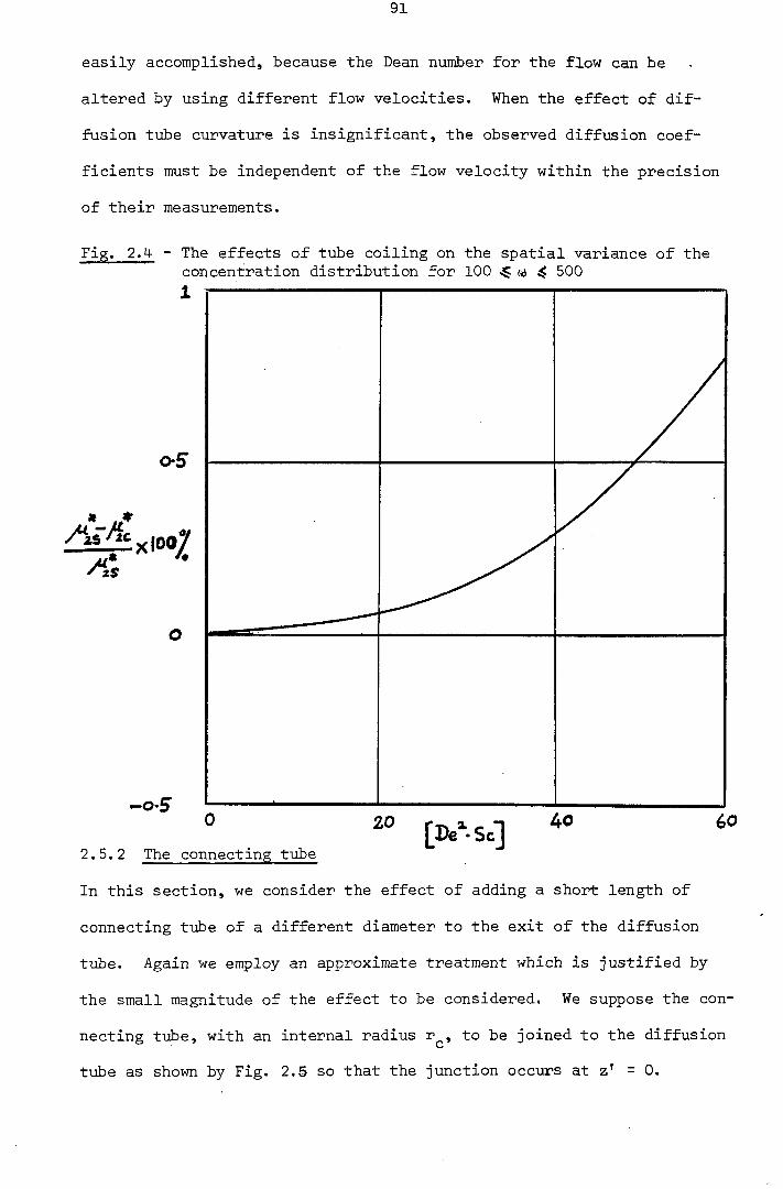
91

easily accomplished, because the Dean number for the flow can be

altered by using different flow velocities. When the effect of dif-

fusion tube curvature is insignificant, the observed diffusion coef-

ficients must be independent of the flow velocity within the precision

of their measurements.

Fig. 2.4 - The effects of tube coiling on the spatial variance of the concentration distribution for 100 w 4 500

o5

zS

0 20 40 60

2.5.2 The connecting tube

In this section, we consider the effect of adding a short length of

connecting tube of a different diameter to the exit of the diffusion

tube. Again we employ an approximate treatment which is justified by

the small magnitude of the effect to be considered. We suppose the con-

necting tube, with an internal radius r^, to be joined to the diffusion

tube as shown by Fig. 2.5 so that the junction occurs at z' = 0.

92

Fig. 2.5 - The connecting tube between the diffusion tube and the refractometer

We assume that there is a sharp transition in the flow pattern in the

tube from the fully-developed profile of laminar flow in the diffusion

tube to that fully-developed profile characteristic of the connecting

tube. From the continuity equation we have

2 ^c^o

where u^ is the mean flow velocity in the connecting tube. It is

further assumed that the diffusion tube and the connecting tube extend

to infinity in either direction about z' = 0 , and that the concentration

distribution resulting mainly from dispersion in the diffusion tube is

observed as a cross-section average at z' = Si, In order to obtain the

concentration distribution observed at z' = £, as a result of a sample

injection into the diffusion tube, again we use the Taylor approximation.

That is, in each tube the diffusion process may be described by the

one-dimensional equation (2.31). Hence we ignore any transient effects

in the entrance region to the connecting tube. In particular, we define

the effective diffusion coefficient by

r^u? _ C O

48D 12

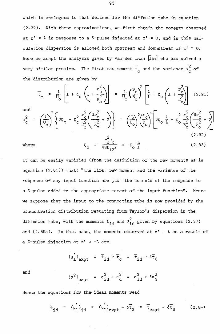
93

which is analogous to that defined for the diffusion tube in equation

(2.32). With these approximations, we first obtain the moments observed

at z' = & in response to a 6-pulse injected at z' = 0, and in this cal-

culation dispersion is allowed both upstream and downstream of z' =0.

Here we adapt the analysis given by Van der Laan [l6^ who has solved a

— _ 2 very similar problem. The first raw moment t^ and the variance of

the distribution are given by

U •

2 r

and

2

o \ o

where 480^2*

(2.81)

_ o \ o

(2.82)

(2.83)

It can be easily varified (from the definition of the raw moments as in

equation (2.61)) that: "the first raw moment and the variance of the

response of any input function are just the moments of the response to

a (S-pulse added to the appropriate moment of the input function". Hence

we suppose that the input to the connecting tube is now provided by the

concentration distribution resulting from Taylor's dispersion in the

diffusion tube, with the moments t^^ and given by equations (2.37)

and (2.39a). In this case, the moments observed at z' = & as a result of

a 6-pulse injection at z' = -L are

^^l?expt *id + = tld + '^3

and (a2)

expt "L 'I "Id + '"l Hence the equations for the ideal moments read

tid = '"I'ld = - " 3 texpt - (2.84)

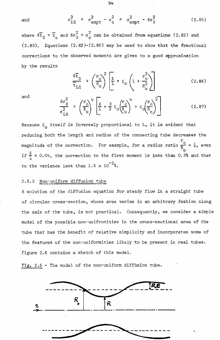
9^•

and 2 _ 2 2 _ 2 - 2

^id ^expt ^expt ^3 (2.85)

where 5tg = and 60^ = can be obtained from equations (2.82) and

(2.83). Equations (2.82)-(2.85) may be used to show that the fractional

corrections to the observed moments are given to a good approximation

by the results

-id R

( 2 . 8 6 )

and

! l 3 2

' id I + I ^o F (2.87)

Because itself is inversely proportional to L, it is evident that

reducing both the length and radius of the connecting tube decreases the r

magnitude of the correction. For example, for a radius ratio — = q, even Z . °

if Y = 0.04, the correction to the first moment is less than 0.3% and that

to the variance less than 1.5 x 10 -2g.

2.5.3 Non-uniform diffusion tube

A solution of the diffusion equation for steady flow in a straight tube

of circular cross-section, whose area varies in an arbitrary fashion along

the axis of the tube, is not practical. Consequently, we consider a simple

model of the possible non-unifromities in the cross-sectional area of the

tube that has the benefit of relative simplicity and incorporates some of

the features of the non-uniformities likely to be present in real tubes.

Figure 2.6 contains a sketch of this model.

Fig. 2.6 - The model of the non-uniform diffusion tube.

95

The radius of the cross-section of the tube is assumed to vary sinusoi-

dally according to the equation

R(z) = ^ + e sin (2.88)

We presume that the amplitude of the oscillations is small,

g « 1

the wavelength is large compared to the radius,

X » R

but it is much smaller than the tube length L,

X « L

In line with our earlier arguments, we seek to analyse the diffusion

process in this non-uniform tube in an approximate manner. So our aim

is to obtain the moments of the concentration distribution in the tube as

a perturbation to those in a uniform tube with a constant radius R^ for

the same volumetric flow rate. Accordingly, we restrict our discussion

to flows for which the lubrication approximation is valid, i.e.

^ « 1. These flows are usually employed for the measurements in

order to ensure laminar flow and satisfaction of condition (2.30). In

Re

this case, the Navier-Stokes equations reduce to the form ]j.60

E = " H ^ and

3U

where cylindrical symmetry has been used and U and U represent the axial

96

and radial components of the fluid velocity respectively. Since

< 3^U^/3r^ by a factor of order (R^/X)^, we may neglect the

former term completely for the conditions specified above. In this

case we easily obtain the solutions for the two velocity components,

correct to order eR^/A, as

(r, z) = - ^ \l - I (2.89) irR

and 4QR E rr,-r.\ Up (r, z) = 2 (jT"' I ~ I (2.90)

where Q is the constant volumetric flow rate through the tube.

Anticipating that the concentration distribution in the tube is cylin-

drically symmetric, as it was for the uniform tube, the diffusion

equation now takes the form

, 3(AC, ) , . / 3AC,"\ 3^WC. ) 340, SAC,

The boundary conditions are, at t = 0,

AC^(r, 0, 0) = 6(z)(C^^ - C^^)

3(AC^) and — ^ — = 0 at r = R(z) for all t (2.92)

where 3/3v indicates differentiation along the normal with respect to

the tube wall. We now write the velocity components and the concentration

distribution for the non-uniform tube as perturbations to those for the

uniform tube, so that

U^(r, z) = U^(r) + eU^ (2.93)

U^(r, z) = eU^ (2.94)

and AC^ = AC° + ec' (2.95)

where the subscript or superscript 'o' denotes the concentration distri-

9 7

bution in the uniform tube. Expansion of equations (2.89) and (2.90)

then shows that

2" U = -4U sin z o (¥)

and U

4U R o o

" ( x

1 - 2

R I— o

R

3 - 1

o / —I

(2.96)

(2.97)

where is the mean flow velocity in the uniform tube. For the condi-

tions of interest, the contribution of axial molecular diffusion to the

dispersion process is considered negligible as before. Consequently,

9 9

following Taylor [l4^ we neglect the term 3 (ACj_)/9z in equation (2.91),

Making use of the fact, to a very good approximation [l48, 23J , that

9(AC^)/3z is independent of r. Hence the diffusion equation (2.91) for

a uniform tube (i.e. to zeroth order in E) is just that given by

Taylor [l4^. The temporal moments of the solution of this equation,

averaged over a cross-section, are therefore the ideal moments given by

equations (2.37) and (2.39a). To obtain the moments of the solution to

first order in e, we employ equations (2.93)-(2.95) in the diffusion

equation (2.91). Again we neglect the longitudinal molecular diffusion

term. Collecting terms of e, we find the following equation for the T

concentration distribution perturbation c in the non-uniform tube:

. . . . , 3(AC°) , 3(AC°)

If- - ".(r) 1 ^ t UJr) t 0^ = D 12 r 9r 9r J

(2.98)

To the same order in e, the boundary condition of no molecular flux

through the tube wall can be shown to be equivalent to

3(AC^)

9r = 0 (2.99)

This is because the curvature of the wall, to first order, depends

linearly on the product of e with R^/X. But R^/X itself is presumed

small so that the curvature is essentially only a second-order effect.

98

Now because 8(AC°)/3r is small and U^/U^ = 0(R^/X) then 3(AC°)/3r <<

3(AC°)/9z. This justifies the neglect of the first of these terms

in diffusion equation (2.98) for the concentration distribution pertur-

bation c'. Averaging equation (2.98) over a cross-section of the tube,

and making use of boundary condition (2.99), we obtain

3c' f , 3(AC°)\ 3c'

--3;--^;+ Uo(r) BE- = 0 (2-100)

where subscript 'm' denotes a concentration averaged over a cross-section.

In order to evaluate the remaining cross-section averages, again we make

use of the Taylor approximation ^48]that 3(AC°)/9z is indistinguishable

from (3AC°^/3z), where AC°^ is the cross-section averaged concentration in

the uniform tube. The same approximation is made for 3c'/9z so that we

obtain the final differential equation as

3c —, / 9AC ^ /3c \

Here, v^ is the mean velocity in the diffusion tube, and U (z) is the

first-order perturbation to it in the non-uniform tube. Averaging the

equation (2.89) over a cross-section yields

u ' = -2v s i n ( 2 . 1 0 2 )

Z O A

which is identical to the result found by Thorsness .

Now taking Laplace transform of equation (2.101), we obtain t —I

It now follows from equation (2.95) and the definition of the temporal

moments of a distribution that, to first order in e, the raw moments in

the non-uniform tube are related to those in the uniform tube by the

expression

99

where is proportional to e and represents the perturbation to the

ideal moments of the uniform tube. Using the results [iS^ that

, d^c'

we can employ equation (2.103) to construct differential equations for the

perturbation to each moment. Differentiating equation (2.103) once with

respect to s, reversing the order of differentiation, and taking the limit

as s 0, we obtain for the first moment

f

(Id) = ° (2.105)

and after two differentiations of equation (2.103), we obtain in the

limit s 0,

i (^2)id - *^l,4 = ° (2.106)

Equation (2.105) is readily integrated using equation (2.102) for U ,

and equation (2.37) for t^^ to yield the perturbation to the first

moment at z = L as

eX r f: 1 - COS I-

. V L I 2TTL\

L' I ^ o

(2.107);

where the boundary conditions reveal that 6y^ ^ = 0 at z = 0, a fact

which we have used. Equation (2.106) can be integrated using equation

(2.38) for (W2)id yield at z = L

' \ r /o-An (2.108)

' V TTV 8ttD _v \ o 12 o

/2ttL 1 - cos I—-—

The first temporal raw moment observed in the non-uniform tube is therefore

100

o 1 +

2nL, £X(l-cos )

X

TTL(1 + 2Gg) (2.109)

and this result together with equations (2.104) and (2.108), and the

2 ' ' 2 definition of the veiriance (a )^^ = ^^2^nu ~ ^^l^nu' he used to

determine this central moment to first-order in e as

(.2) nu = (1)' 8C^ + 2C

eX(l-cos

1 + TTL(1 + 4;^)

(2.110)

so that

6a, 2eAC L

TT 1 - cos (¥ (2.111)

From equations (2.109) and (2.110) it is clear that under practical

conditions, 5^ « 1, the correction to both moments is of order e .

Because e << 1 and << 1 for the most likely practical situations, the

corrections to both moments are small. For example, if the non-uniformity

X

of the tube bore is 1% and = 0.1 then the correction to neither

moment exceeds 0.06%. It was shown earlier that, to a very good approxi-

mation, equation (2.46) may be used to determine the value of For

the non-uniform tube, this equation becomes

12 (2.112)

by virtue of smallness of That is, to first order in e, the effect

of the non-uniformity of the diffusion tube bore upon the moments of the

concentration distribution in the evaluation of the diffusion coefficients

only occurs in small terms (~ 1%) in the complete working equation (2.43).

Furthermore, these effects are themselves very small under the con-

ditions of interest in this work. Hence the overall contribution of

non-uniformity to the evaluation of the diffusion coefficient from the

observed moments is negligible. A final point of significance arising

from the non-uniformity of the diffusion tube concerns the determination

101

of its internal radius R^. It can easily be shown that for the present

model of the non—uniform tube, the volume of the tube to first-order

in £ is given by

eX Vt = Acfj 1 + .L 1 - cos (2.113)

2 where is the tube cross-section area which can be determined

from a measurement of the tube volume and its length. The maximum error

2 . . . A

in the value of R^ calculated in this way is of the order of e -jj, which

in practice can be made negligible by selection of tubing of a suitable

quality (see Section 3.2.1).

2.5.4 Non-circular cross-section

As in the case of the preceding section, we consider the effects of the

non-circular cross-section of the tube by means of a particular model.

We assume that the tube has an elliptical cross-section with major and

minor semi-axes a^ and a^ respectively. The eccentricity e is given by

t-eTT (2.114)

Taylor dispersion in such a tube has been studied by Aris [l4^. From

his work it can be shown that in such a situation the simplified

working equation (2.46) for circular tubes must be replaced by the equation

ry \ 2 ' f(e)a y

D = (2.115) 24a

e ' 2

where and are the first raw temporal moment and the variance

observed in the elliptical tube respectively, and

f(e) = ~ (2.116) 24 - 12e

In practice, it is not convenient to determine the ellipticity of a tube

or the semi-axes directly. But it is possible to measure the tube volume

and its length so as to determine its cross-sectional area A^ where

102

Ag = IT = IT a^(l - e (2.117)

Therefore we consider the result of evaluating the diffusion coefficient

» 2

from experimentally determined moments and 0^ in an elliptical tube

by means of the equation

e A %ie D®2 = 2 (2.118)

24ir a e

The ratio of the diffusion coefficient calculated for the elliptical

tube, to true value, is

Expanding the ratio in powers of the eccentricity, e, we find that

^ = 1 - ir + ... (2.120) ^12

which indicates that for small eccentricities, we can equate D^2 to D^2

without introducing any significant error. Numerical evaluation of the D a

ratio through equation (2.120) shows that when e = 0.2 ( — = 0.98) °12

the ratio departs only by 0.01% from unity. Therefore, as long as the

tube cross-sectional area is determined experimentally, we can use

equation (2.118) to interpret the experimental data even if the diffusion

tube has an elliptical cross-section.

2.6 Concentration-Dependent Fluid Properties

In all of our analyses so far, we have assumed that the properties of

the fluid mixtures involved are independent of composition. In this

section, we examine the consequences of the fact that both the diffusion

coefficient to be measured and the mixture density depend upon composition.

Because the injected sample is necessarily of a different composition from

103

that of the flowing stream, the density of the mixture will vary from

point to point in the diffusion tube. This may possibly cause natural

convective flows. Besides, the composition dependence of iirplies

that we should re-examine our solution of the diffusion equation for

this case.

2.6.1 Concentration-dependent diffusion coefficient

Because it is not possible to solve the dispersion equation (2.2) for the

case when is a function of C^, we consider instead an approximate

analysis based upon that originally given by Taylor [l4^ . That is, we

again recognise that to a very good approximation, under the present

conditions of interest, the dispersion process may be described by a

one-dimensional diffusion equation. An equation which describes the

evolution of the cross-section averaged composition which is characterized

by the effective diffusivity

^ ~ (2.121)

which is now supposed a function of C^, is proposed. Following Taylor

[iM-S]] we can then write the diffusion equation in the form

9t 9C\

where ^ is the axial distance with respect to the moving origin defined

by equation (2.6). The initial condition for the solution is the

injection of a 5-function pulse at z = 0 at time t = 0.

Suppose that the composition dependency of can, over a suitably

small composition range, be represented by the equation

where is the diffusion coefficient at the composition of the flowing

104

stream. Thus we have

E(iC^^) = E (1 + X 4Cj_^) (2.124)

where E is the effective diffusivity at the composition of the flowing

stream. A perturbation solution of equation (2.122) with E given by

equation (2.124) has been given by Hopkins . The first-order per-

turbation solution reads

ACim(X' t)

N X

^ 1 + .. 3 / 2 , _ o 1 4TT

exp

g/lT

(E"t)2

/ »2\

4E°t yj

2(E°t)2 T erf

.2(E°t)2

(2.125)

Here, is the solution when E = E° is a constant, i.e.

N. AC

Im (2*3/2(Eot)lR2

exp 4E°t

(2.126)

where N^, as defined by equation (2.1), represents the number of moles

of species 1 in the injected sample in excess of those present in the

same volume of the flowing stream. The first and second spatial

moments of this perturbed distribution can readily be evaluated with

respect to the moving origin to lead to the results that

0

and

y''' = 2E°t 1 t N

1 + i" ^

nR^(2E°t)2 o

(2.127)

which can be written as

(2.128)

where

E(Clr) 1 + X — : — r nRg(2E°t)2

(2.129)

105

so that E(C^^) is the value of E at a composition

" aT?' 'ir = 'if '

From equations (2.121), definition of E, and (2.128) we have

^2 ~ 24D^^TC^ (2.131)

which has exactly the same form as that of the working equation (2.25)

derived for the case of constant diffusivity. Hence we conclude that if

we employ equation (2.25) or its equivalent in terms of temporal moments

(equation (2.4-3)), the diffusion coefficient obtained should be referred

to the composition given by equation (2.130) and not to the flowing

stream composition. But because modern composition monitors, such as

the refractive index detector, are extremely sensitive to composition

changes, can usually be made very small. In this case, the departure

of the reference composition from that of the flowing will be insignificant.

2.6.2 Concentration-dependent density

We now consider the consequences of the fact that the density of the

liquid sample mixture injected into the flowing stream necessarily differs

from that of the flowing stream. Assuming that the concentration dif-

ferences are small, the density p at any point in the tube may be con-

sidered to be a linear function of the concentration. So we can write

p = pf(l + Y AC^) (2.132)

where p^ is the flowing stream density. The occurence of density dif-

ferences in the diffusion tube introduces two new effects in the dis-

persion process. First, the longitudinal density gradients lead to

longitudinal pressure gradients which modify the velocity distribution in

the flow. Second, due to radial density gradients, buoyancy forces are

106

induced which drive a secondary flow. An exact analysis of the equations

of fluid mechanics which govern this situation is not available. But

Erdogan and Chatwin [l5^ give an approximate treatment based upon the

assumption of small density changes. Their analysis is restricted to

the region where the Taylor dispersion process becomes one-dimensional.

Under these conditions, they found that the evolution of the cross-section

averaged concentration in the tube was controlled by the equation

3-1 3AC

Im at 480^2 95

9C

s r - •'"2

'3AC Im^

35 (2.133)

Here depends on the Peclet number, Pe, where

Pe = R U o o D

(2.134) 12

and the Schmidt number defined by equation (2.75)

, 1 -.2 ^2 ^288Cr

Sc

Pe _

(2.135)

The parameter <j) is defined in terms of the coefficient y by the equation

2

(j)' r Y g Rq

2 n _i

(2.136)

where g is the acceleration due to gravity and n is the fluid viscosity.

Approximate solutions of equation (2.133), based on one-dimensional Taylor

dispersion, have been obtained by Barton [1723 and Smith [i7:^ . They have

used the results to derive expressions for the spatial variance of the

concentration distribution. Smith's expression reads

"2 - 2W^ 2 "IT ^3r6U233/2^ o o

(2.137)

where is the variance at the end of a transient period when the

asymptotic solution becomes valid. This transient region has never been

analysed and hence equation (2.137), which is itself approximate, cannot

1 0 7

be used to provide the corrections to the observed moments. Also it

does not give any guidance as to when buoyancy effects may be neglected.

However, it does provide means of deciding whether or not buoyancy

effects are significant in particular measurements. That is, if we use

equation (2.27), the working equation for the ideal experiment, to

determine the diffusion coefficients from experimentally measured spatial

moments under significant buoyancy effects, then equation (2.137) shows

that the resulting apparent diffusion coefficient (D^^)^ , will differ

from its true value „,

_ — I -1

1 , ^ ^°12^p " °12

R^U^t TT^RVa^^^t^ o o o o

(2.138)

Therefore, the apparent diffusion coefficient would depend upon the flow

velocity U^, time of measurement t, the excess number of moles N^, injection

and the magnitude of the initial concentration perturbation. On the

other hand, if such dependencies are absent in the measurements, it

implies that the experimental data are free from errors due to buoyancy

effects. In order to ensure that the buoyancy effects are eliminated

from our experiments, we must carry out measurements over a wide range

of flow velocities and injection concentrations. Because buoyancy

effects are minimized as the difference between the injection and flowing

stream concentrations diminish, we,must always use injection samples with

concentrations as near as possible to that of the flowing stream.

2.7 Summary of the Theoretical Analysis

The foregoing analysis has shown how, under the appropriate conditions,

it is possible to design an apparatus to measure liquid phase diffusion

coefficients that departs only in small respects from its ideal model.

Some of the departures from the ideal can be rendered so small as to be

108

negligible. Other effects, although not negligible, may be made suitably

small by the design so that corrections may be applied to account for them

with confidence. We conclude this chapter by summarizing the results

for the convenience in the design and use of such an apparatus.

Among the effects that can be rendered negligible are those which arise

from the coiling of the diffusion tube and non-uniformity. In order to

eliminate coiling effects, conditions must be chosen such that

[pe^.Sc) $ 20

and that 100 $ w = I j $ 500

The non-uniformities of the diffusion tube bore are insignificant pro-

vided that the amplitude of the radius fluctuations, eR^, and the length

scale of their fluctuations are such that

4 < 1°"'

In view of both non-uniformities of the cross-section and its possible

non-circularity, the effective cross-sectional area of the tube, A^,

should be determined by measuring its length and volume. This measure-

ment then renders effects due to any ellipticity in the cross-section

negligible, provided that 2 i

e = ['-©] • -Buoyancy effects have not been accounted for exactly in the discussion,

although an experimental method of checking and eliminating their con-

tribution to the dispersion process has" ibeen proposed.

In addition, provided that conditions are chosen to satisfy the require-

ments of laminar flow,

2R U Re = — — < 2000

109

and the additional constraints

in which case

and

t ) 20

10 - 3

I "o ^

the working equation for the determination of the diffusion coefficient is

12 24*t.

5 + J(1 - 5^) ']

where

6^ = (768)^K$Q

K = 2.1701 ... X 10 -5

and

4 d -

In these expressions, and are the temporal first raw moment and

the variance (equal to second central moment) in an ideal experiment.

They may be obtained from measurements of the same moments in a real

— 2 experiment, t^^^^ and by application of the equations

"•id 'expt - Z 61__ n n

and •

2 " id expt

- S 6a' n n

110

where 6t and 6CT are small corrections due to the departures from the n n ^

ideal, and for the present, they include

1. The corrections due to the Refractive Index Detector used to monitor

the concentration distribution at the exit of the diffusion tube

r/v. 6t.

60' U

t tR L

TTR L

2. The corrections due to the Sample Introduction by Rectangular Pulse

Injection

'K'ol \ o /

2

) 3. The corrections due to the Connecting Tube between the diffusion tube

and the refractive index detector

12 VU irR L

'^3 = ( -0/ v^o

do! " 4 ) • ' • ft) ft • "

In addition, the molar concentration of species 1 in the mixture to which

the measured diffusion coefficient refers is C^^, given by the equation

= Clf "

where 6Cj is a further correction to the flowing stream concentration C^^

and may be obtained from

SC ^ l ^ l l " 8 ^ )

r

for an extra number of moles, N^, of species 1 injected.

Ill

Finally, it is important to record that the use of a laboratory metering

pump may appear to be a convenient choice for maintaining the

constant flow rates through the diffusion tube. But such metering

pumps can result in severe short time pulsations which could affect the

laminar dispersion significantly. It has been found [l67] that the effec-

tive diffusion coefficient under pulsating flow conditions could be

higher, equal to, or less than, that for non-pulsating flow, depending

on the experimental conditions. Therefore, the use of a gravity feed

supply (see Section 3.4) to maintain the constant fluid flow rates

through the diffusion tube will eliminate any errors introduced into

the measurements due to this effect.

It will be shown in the proceeding chapter how the sometimes conflicting

conditions for a suitable design can all be satisfied in a practical

apparatus. It will also be verified that the residual systematic errors

in the application of the Taylor Dispersion Method have been reduced to

a level below that of the random errors of measurement.

112

C H A P T E R S

APPARATUS AND EXPERIMENTAL PROCEDURE

3. Introduction

The theoretical analysis of the previous chapter has been employed for

the design and operation of the equipment used in this work. The

instrument has been designed to operate in a wide temperature range,

10 - 200°C, at atmospheric pressure. The general features of the

apparatus and the experimental procedure adopted are described below

and subsequently individual items are discussed in more detail.

3.1 Apparatus Design

The function of the apparatus design was to determine the conditions of

the experiment and dimensions of the instrument so that the departures

from ideality, mentioned in the preceding chapters, contribute as little

as possible to the measured diffusion coefficients. The geometric, mecha-

nical, thermal and electrical characteristics of the equipment were there-

fore selected following a careful design study based upon the previous

theoretical analysis. As a result of this study, an instrument has been

designed which satisfies all the necessary conditions arising from the

theory of the method and whose precision is one of ±0.5%. To attain this

precision, all of the corrections for the first moment and the variance

of a distribution have been constrained to be less than ±0.6% of the

ideal moments. Because these corrections may be estimated to within ±5%,

the residual uncertainty arising from each correction is therefore no

more than ±0.03%. The design of the instrument together with the theory

of its operation, ensure that systematic errors are negligible. Including

errors in the measurement of the geometry of the diffusion tube, the

accuracy of the diffusion coefficient is estimated to be one of ±1.0%.

113

Figure 3.1 shows a schematic diagram of the diffusion equipment whose

flow diagram, Fig. 3.2, is presented later.

The diffusion tube, 1, whose length is 13.219 metres is made from 0.8198

millimetre internal diameter stainless steel tubing (Phase Separations,

Ltd.) wound on a copper former, 2, by means of four equidistant copper

pillars and embedded in lead, 3, to provide thermal stability. The tube

is carefully wound round the pillars such that a smooth coil is obtained

without any indentations or sharp comers. A modified liquid chromato-

graph injection valve, 4, Figs. 3.4-3.7, (Analytical Accessories, Ltd.)

and the tube are contained in a copper isothermal enclosure. Fig. 3.8,

fitted with q—inch I.D. bifilar copper pipes, 5, for the circulation of

a heating fluid. An ultra thermostat circulating bath (Lauda - model

NB-S 15/12 with universal relay unit R2 electronics) is employed for this

purpose. The outer surface of the block with pipes is coated with a thick

layer of lead, it is then jacketed by a highly insulating material, 2.5

inches thick (ICI). Thermal equilibrium is reached throughout the block

after several hours of circulation of the heat exchange fluid. The tem-

perature of the diffusion tube is measured with the aid of four iron-

constantan thermocouples, 6, inserted into the lead support through the

four equidistant copper pillars. An extra thermocouple measures the tem-

perature of the injection valve to ensure that it is at the same tempera-

ture as the diffusion tube. All thermocouple junctions are electrically

insulated by 'shellac' coating so as to prevent metal-to-metal contact.

The temperature stability and uniformity is approximately ±0.05 °K over

a period of several hours.

The fluid flow through the diffusion tube is maintained by a gravity

feed, 7, from a reservoir, 7 , which is designed and arranged so that

the liquid level change during the course of a single measurement is

negligible, hence the flow velocity remains constant during a particular

114

run (Section 3.4). The liquid flows from the reservoir, Y, to the

injection valve through a preheater, 8, fourteen turns of tubing iden-

tical to the diffusion tube wound on a copper rod, to ensure thermal

equilibrium before injection of the solute sample^lO'The effluent from

the diffusion tube is fed to a differential refractometer, 9, (Waters

Associates Inc.) employed for the detection of the eluted distribution.

More details about :the design or specifications of various parts of the

equipment and its operation and performance are contained in the follow-

ing sections.

3.2 The Diffusion Tube

The diffusion tube is the most important part of the equipment and

therefore requires special consideration both in the selection of the

material, and in the selection of its dimensions.

3.2.1 Material of the tube

The material from which the tube is constructed must be inert so as to

ensure that chemisorption and physisorption of the species do not occur,

even though the liquid alkanes used are saturated hydrocarbons and inert

themselves. A relatively high thermal conductivity is essential for the

rapid and efficient transfer of heat to the liquids flowing through it,

without any phsyical or chemical deformation of the tube at high tempera-

tures. The theory of the method indicates that a smooth, straight tube

of several metres with circular cross-section is required. However, for

reasons of practicality, such a long tube must be coiled in a helix of as

large as possible radius with negligible variation of cross-section along

its entire length.

In order to meet all the requirements mentioned above, drawn 316 stain-

less steel tubing was chosen (Phase Separations Ltd.).

115

Fig. 3.1 - Schematic diagram of the diffusion equipment

-I -: (2)

r r m

\ \ \ \ \ \ N

116

Fig. 3.2 - Flow diagram of the diffusion experiment

5P w K

w II Z

HS

r-MEr

I

Va

D yyyyyA

Vb

7ZZZZ

4 3 = M a

\2zz T 7 x E ? x r . .

t t t 7ZZZZ2ZZZZZZ2^

II w

L / V

-r- t w w © Q © — J —

i w

© o

© © © - T "

M

Fig. 3.3 - Schematic diagram of the injection value operation

FILL POSITION

solute loop

solute from B in f

out

INJECT POSITION

solute loop

solute solvent from from B

A in » solvent from A

to the diffusion tube

out to the diffusion

tube

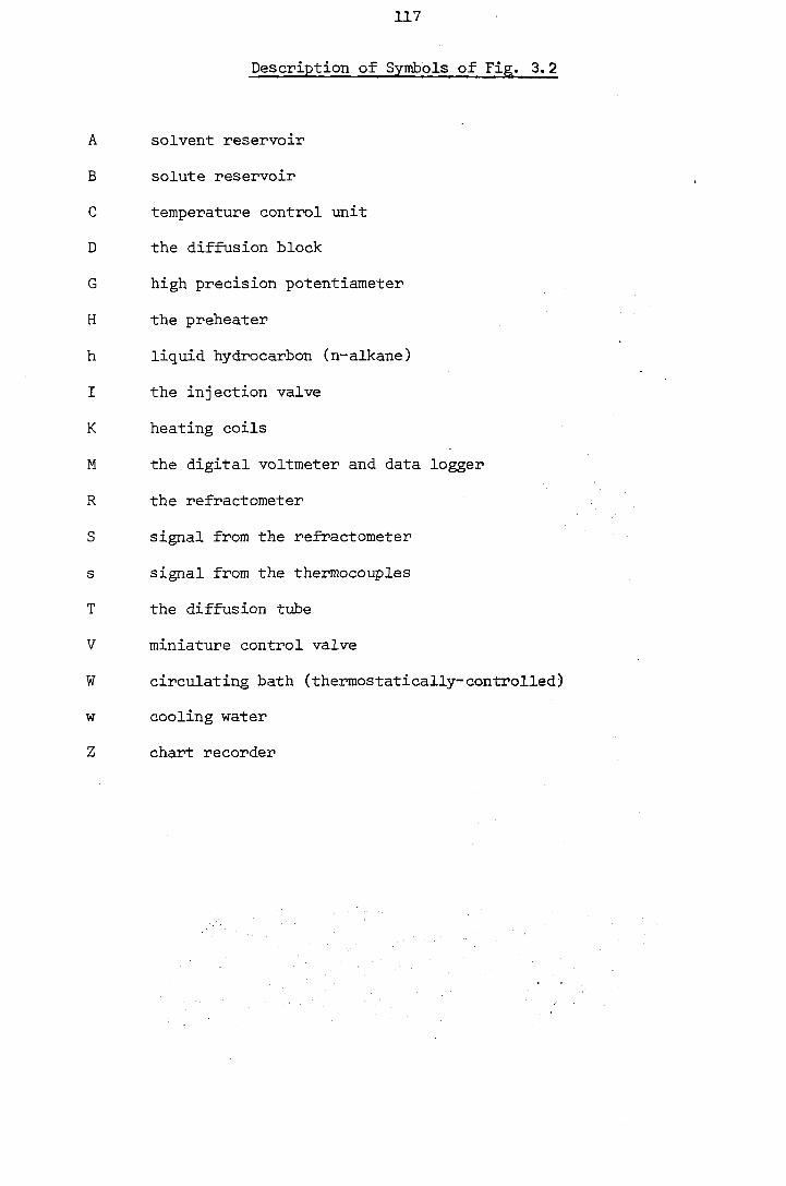
117

Description of Symbols of Fig. 3. 2

A solvent reservoir

B solute reservoir

C temperature control unit

D the diffusion block

G high precision potentiameter

H the preheater

h liquid hydrocarbon (n-alkane)

I the injection valve

K heating coils

M the digital voltmeter and data logger

R the refractometer

S signal from the refractometer

s signal from the thermocouples

T the diffusion tube

V miniature control valve

W circulating bath (thermostatically-controlled)

w cooling water

Z chart recorder

0 4 . 2 5

QC)

00 O

Osl @ l

3 5

s i

IMS

0 6 - 5

0 9 - 5

00

Fig. 3.H - The injection valve

(all dimensions to scale in mm)

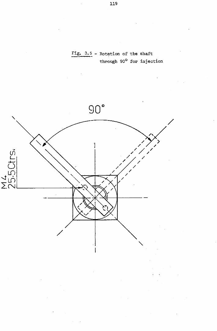
119

Fig. 3.5 - Rotation of the shaft

through 90° for injection

90

\

s. ' \

V V

/

Fig. 3.6 - The injection valve with the sample loop

10 microlitre sample loop

y — y k 1 — 14 •«

Vr. i

L l i

Fig. 3.7 - The conical rotor

rviro

lO

0 Z . - 7 5

122

Fig. 3.8 - The isothermal diffusion block

(all dimensions in inches - not to scale)

123

Description of Symbols of Fig. 3.8

A copper screw cap

B Teflon conical seal

C copper bracket

D copper pillar

E port for solvent and solute tubes and thermocouples

F bifilar copper tubes for heat exchange

I copper block isothermal enclosure

L diffusion tube assembly

F solvent preheater

R diffusion tube exit port

T diffusion tube

V injection valve

124

3.2.2 Design study for optimum geometry of the diffusion tube

As indicated earlier, the object of the design study is to choose opera-

ting conditions such that the departures of the real apparatus from the

ideal are either rendered negligible or small and amenable to calculation.

Considering the theoretical analysis in Chapter 2, various criteria must

be applied to the mathematical model for diffusion, i.e. to the working

equation (2.46)in order to ascertain the appropriate conditions for opera-

tion. Because various requirements are often conflicting, it is neces-

sary to search for the optimum dimensions of the diffusion tube subject

to these constraints. The important constraints are:

(l) Time of measurement

(a) Immediately following the injection of a pulse of material into the

flowing stream, there is a period of transient behaviour as shown by

eqns*(2»15—16)-The time 't^',which must elapse before the transient contri-

butes a negligible amount to the final eluted concentration profile is

given by Taylor/Aris criterion [l8, 148, 14^

2 lOR

•'a >

<='" 10"'

This criterion satisfies c o n d i t i o n w h i c h makes the transient terms

of eqns^2-15'^6)unimportant. Thus, in order to operate in a region where

the initial transient diffusion process is negligible, i.e. Taylor's

region, the time of measurement should exceed the value 't^' which is

a lower time limit in a given diffusion tube with a fixed diffusivity.

(b) On the other hand, for reasons of experimental convenience, and

to achieve the necessary temperature stability, a measurement time should

not be allowed to exceed four hours (14 Ks).

125

It has already been mentioned that the diffusion tube is several metres

long. Thus it cannot be kept straight and thermostatted satisfactorily

and must be coiled. This coiling is a cause of secondary dispersion effects

[21, 29, 158, 16(^ , but these can be kept within the desired limits '

by an appropriate choice of flow velocity. The diffusion peak must be

attained within a few hours so that the measurement may be performed in

a reasonable time. These latter points are significant, but cannot be

allowed to dictate the design since, in principle, the tube coiling may

be made of any necessary radius to render secondary dispersion negligible

and the experiment duration can, if necessary, be extended.

(2) Reynolds Number 'Re' of the flow

In order to ensure that the flow velocity profile in the diffusion tube

is parabolic as required for the laminar flow, conditions must be chosen

to satisfy this requirement, i.e.

2R U Re = — — < 2000

V

(3) Dean's Number 'De' of the flow

The Dean's Number of the flow for the diffusion experiment is defined as

. a De = Re

In order to eliminate the coiling effects, conditions must be chosen so

that

2 [be .S^ ^ 20

and that rR'

100 ^ 1 $ 500 o

Thus it is desirable to work with a Reynolds Number which is as low as

possible. The results of the design calculations in Section 3.2.5 show

that a suitable criterion is

Re 3 6

126

(4) Magnitude of the corrections of the experimental moments

The ideal moments of the solute distribution are determined by correc-

ting the experimental moments as shown in the previous Chapter. The

relative corrections to the first moment are due to the injection volume

V^, the detector volume V^, and the connecting tube volume V^. They

become insignificant if

Vi 3 0.01

2ITR^L O

V, g 0.01

2 irR L

o

V ° 3 0.01

TTR^L o

The corrections to the second and higher moments depend upon the square

and greater powers of those for the first moment. Consequently, the

corrections to these higher moments become negligible (less than 0.01%)

when the corrections to the first moments are less than ±1% and c; is

less than 10

As explained in the previous Chapter, it is only possible to connect the

diffusion tube to the refractometer by coupling the former with a con-

necting tube. This is a 316-stainless steel tube of 0.2 mm nominal

internal diameter and 35 cm long, coupled with the diffusion tube by means

of a zero dead-volume union. It is fixed to the refractometer and connec-

ted to the entrance of the sample cell internally which makes it diffi-

cult to handle. Corrections due to this effect will not introduce sig-

nificant error if

irr i V = - f - = ^ 0.01

ttR L TTR L o o

for r = 10 ^ m, & = 0.35 m and Z $ 10 c o

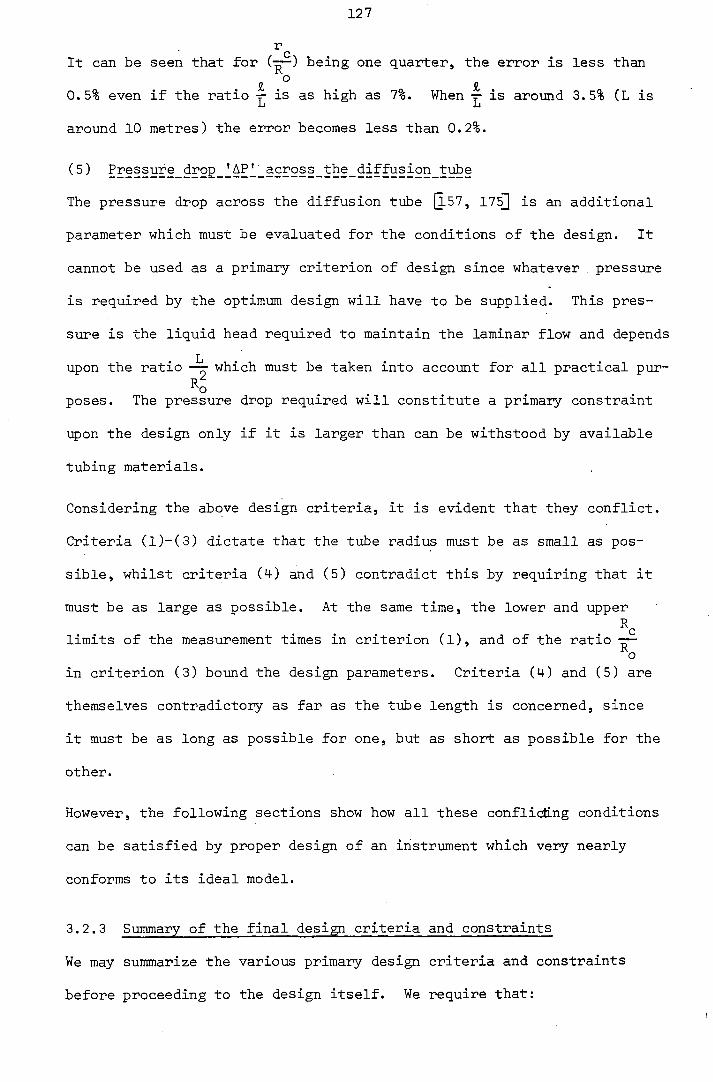
127

It can be seen that for ( — ) being one quarter, the error is less than & ° &

0.5% even if the ratio is as high as 7%. When is around 3.5% (L is

around 10 metres) the error becomes less than 0.2%.

(5) Pressure drop 'AP' across the diffusion tube

The pressure drop across the diffusion tube [157, 175^ is an additional

parameter which must be evaluated for the conditions of the design. It

cannot be used as a primary criterion of design since whatever pressure

is required by the optimum design will have to be supplied. This pres-

sure is the liquid head required to maintain the laminar flow and depends

upon the ratio which must be taken into account for all practical pur-

poses. The pressure drop required will constitute a primary constraint

upon the design only if it is larger than can be withstood by available

tubing materials.

Considering the above design criteria, it is evident that they conflict.

Criteria (l)-(3) dictate that the tube radius must be as small as pos-

sible, whilst criteria (4) and (5) contradict this by requiring that it

must be as large as possible. At the same time, the lower and upper

limits of the measurement times in criterion (l), and of the ratio — o

in criterion (3) bound the design parameters. Criteria (4) and (5) are

themselves contradictory as far as the tube length is concerned, since

it must be as long as possible for one, but as short as possible for the

other.

However, the following sections show how all these conflicting conditions

can be satisfied by proper design of an instrument which very nearly

conforms to its ideal model.

3.2.3 Summary of the final design criteria and constraints

We may summarize the various primary design criteria and constraints

before proceeding to the design itself. We require that:

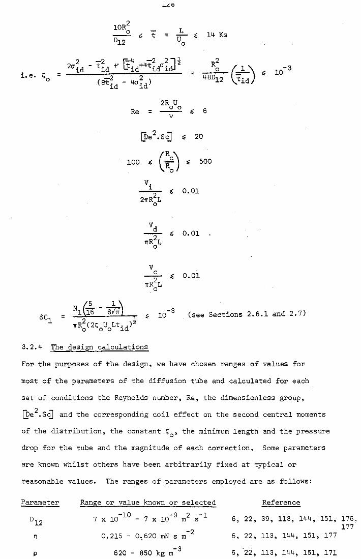
xzo

lORo _ L

2* id - t L ^ ^

^ ( 4 a - - L ) " "

2R U Re = — 2 - ^ $ 6

[be^.Sc] € 20

12 GD' S 10"^

ft)-100 < ( 1 g 500

V. 1

2ITR^L o

_2i_

irR L o

V c 2

TTR L o

$ 0.01

$ 0.01

$ 0.01

QQ - I^IS ^ S 10 ^ (see Sections 2.6.1 and 2.7)

^ "Ro"^o"o"id>^

3.2.4 The design calculations

For the purposes of the design, we have chosen ranges of values for

most of the parameters of the diffusion tube and calculated for each

set of conditions the Reynolds number. Re, the dimensionless group,

[j)e .S( and the corresponding coil effect on the second central moments

of the distribution, the constant the minimum length and the pressure

drop for the tube and the magnitude of each correction. Some parameters

are known whilst others have been arbitrarily fixed at typical or

reasonable values. The ranges of parameters employed are as follows:

Parameter Range or value known or selected Reference

-in _q 9 -1 7 X 10 - 7 X 10 m^ S ^ 6, 22, 39, 113, 144, 151, 175.

_9 177 n 0.215 - 0,620 mN s m 6, 22, 113, 144, 151, 177

p 620 - 850 kg m~^ 6, 22, 113, 144, 151, 171

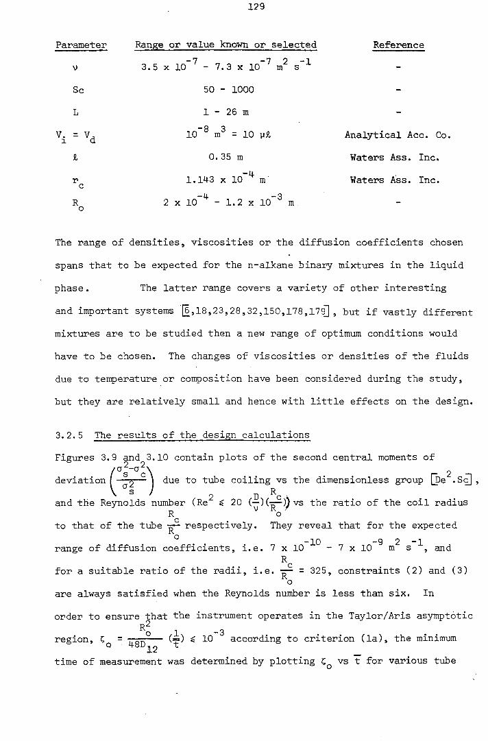
129

Parameter Range or value known or selected Reference

-7 -7 2 -1 V 3.5 X 10 - 7.3 X 10 m s

Sc 50 - 1000

L 1 - 26 m

10 ^ m^ = 10 y5, Analytical Acc. Co.

£ 0.35 m Waters Ass. Inc.

— L|. r 1.143 X 10 m Waters Ass. Inc. c

R 2 X lO"^ - 1.2 X 10~^ m o

The range of densities, viscosities or the diffusion coefficients chosen

spans that to be expected for the n-alkane binary mixtures in the liquid

phase. The latter range covers a variety of other interesting

and important systems [6,18,23,28,32,150,178,179]], but if vastly different

mixtures are to be studied then a new range of optimum conditions would

have to be chosen. The changes of viscosities or densities of the fluids

due to temperature or composition have been considered during the study,

but they are relatively small and hence with little effects on the design.

3.2.5 The results of the design calculations

Figures 3.9 and 3.10 contain plots of the second central moments of

deviation j due to tube coiling vs the dimensionless group [be . S( ,

and the Reynolds number (Re^ ^ 20 (—)(-^)^vs the ratio of the coil radius

R o to that of the tube — respectively. They reveal that for the expected

° . . -10 -9 2 -1 range of diffusion coefficients, i.e. 7 x 10 - 7 x 10 m s , and

R for a suitable ratio of the radii, i.e. — = 325, constraints (2) and (3)

^o are always satisfied when the Reynolds number is less than six. In

order to ensure that the instrument operates in the Taylor/Aris asymptotic

* o 1 - 3

region, C = (=) 10 according to criterion (la), the minimum ° 12

time of measurement was determined by plotting vs t for various tube

130

radii (2 x 10 ^ - 1.2 x 10 ^ m) as shown by Figs. 3.11 and 3.12. From

these two Figures it is clear that the tube with a radius greater than

6 X 10 m would inevitably result in measurement times in excess of

14 Ks disobeying constraint (lb). Figure 3.13 contains the result of

similar calculations for an average tube radius of 4 x 10 m covering

the whole diffusivity range. The minimum time of measurement for each

case corresponds to a minimum length of the diffusion tube which was then

calculated. The result is presented by Fig. 3.14 which, together with the

two previous Figures, give the possible range of the tube radii as

1.5 x 10 ^ m $ ^ 6 X 10 ^ m.

A plot of the total corrections, as in constraint (4), against the tube

radius for three tube lengths of 6 m, 13 m and 20 m is contained in Fig.

3.15. It indicates that the corrections become less than 1% for the

-4

shortest tube only if ) 4 x 10 m, whilst the longer tubes introduce

corrections of less than ±0.5% for the same radius. The difference of the

corrections for the latter tubes become insignificant (less than 0.05%)

for R 5 4 X 10 m and so the shorter tube (13 m) is a better choice. o

Finally, Fig. 3.16, referring to constraint (5), contains the result of

calculations of the pressure drop across various tubes, i.e. L = 6 m,

13 m and 20 m, R^ = 0.2 mm, 0.4 mm and 0.6 mm, at various times of - 1 0 2 - 1

measurement and for the most viscous fluid mixture (D]_2 = 7 x 10 m s ,

-7 2 -1-

V = 7.3 X 10 m s ) considered in this work. It is evident from this

plot that for measurement times in the range 2.5 - 14 Ks, and for the two

tubes whose dimensions are L = 20 m, R^ = 0.6 mm and L = 13 m, R^ = 0.4 mm,

the maximum pressure drop required is 0.23 m of the liquid which is easily

achieved. Due to the material cost and convenience (R^ = 325 R^), the

smaller tube is preferred.

131

Fig. - 3.9 - The effect of tube coiling on the variance of solute

distribution. Constraints (2) and (3).

= variance of the straight tube

a = variance of the coiled tube c

De = Dean's No.

Sc = Schmidt No.

1.0

0. 5

Deviation

r 2 ^ 'a -a s c X 100%

-0. 5

/

Wor Reg

king ion

iLLUH'

20 40

[be^.Scl

60 80

132

R Fig. 3.10 - Reynolds No. vs Ratio ( ~ )

Constraints (2) and (3)

Re = Reynolds No,

R = Ratio of the coil radius to tube radius

Re

R

500

133

Fig. 3.11 - Taylor/Aris criterion for various tube radii

and 0^2 = 7 X 10 ^ s Constraint (l).

1.5 X 10 -3

5 X 10

-9 2 -1 = 7 X 10 m s

vyy/yy/yyyyyy/y///y/////////y'/

Region where Taylor/Aris solution and eqn. (40) apply

t(Ks)

134

Fig. 3.12 - Taylor/Aris criterion for various tube radii -10 9 -1

and 0^2 = 7 x 10 m s . Constraint (1).

1.5 X 10 -3

10 -3

— ij. 5 X 10 H

10 - 6

-10 9 -1 0^2 = 7 X 10 m s

Region where Taylor/Aris ^solution and eqn. (40)

T" 6

— r 10

-r-12 14

t(Ks)

135

Fig. 3.13 - Taylor/Aris criterion for 0.4 mm tube *~10 —Q 2 —1

and = ? x 10 - 7 x 10 m s .

Constraint (1)

1.5 X 10 -3

R = 0.4 mm o

10 - 6

- r 2

Region for Taylor/ Aris solution and eqn. (40)

5 X 10 ,

12 = 7 X 10-9 ^-1

T 6 10

"T"

12 14

t(Ks)

136

Fig. 3. IM- - Minimim tube length required vs tube radius

Constraint (1)

m m

(mm)

137

Fig. 3.15 - Total % correction for tubes of different geometry-

Constraint (4)

1.0

% correction

Vn

0.5-

RQ X 104 (m)

138

Fig. 3.16 - Pressure drop across the tube vs flow time

Constraint (6)

R = 0.2 mm o

R = 0.4 mm o

R = 0.6 mm o

0. 6

AP (m of alkane)

0.3 .J

\ \ \

T(Ks )

139

3.2.6 Conclusions of the design study

-10 -9 2 - 1

For diffusion coefficients in the range 7 x 1 0 - 7 x 1 0 i n s ,

the optimum working design parameters for the diffusion apparatus are:

(1) Length of the diffusion tube - 13 m;

-14. (2) Radius of the diffusion tube - 4 x 10 m;

- g 3 (3) Injection volume - 10 m ;

-8 3 (1+) Connecting tube volume - 1.43 x 10 m ;

- g 3

(5) Detector volume - 10 m ;

(5) Coil radius - 0.13 m;

(7) Measurement times 3.5 - 14 Ks (1- 4 hours). i

Calculations of the effect of tube coiling have been carried out for

C the conditions selected above (Fig. 3.9). They indicate that for a coil

radius of 0.13 m the error introduced into the diffusion coefficient

-10 2 -1

is no more than ±0.05% for a diffusion coefficient of 7 x 10 m s

with a flow time of 7 Ks. Clearly for other diffusivities a flow time

can always be found for which the effect is negligible, with higher

diffusion coefficients requiring shorter flow times, while still satis-

fying the other constraints.

3.2.7 The apparatus constants

The following Table contains the dimensions of the diffusion tube and

other elements of the apparatus.

The length of the diffusion tube (316 annealed stainless steel, 1/16"

nominal O.D.) employed for this work was determined in several indepen-

dent measurements; it was then coiled very carefully round a copper

former into a helix of known diameter. Its volume was determined gravi-

metrically by filling the tube with distilled water several times and

weighing. The average cross-sectional area of the tube was then found

from which the average tube radius was calculated. The geometry of the

140

diffusion tube was such that the computed errors due to non-imiformity

and ellipticity (Sections 2.6.2 and 2.6.3) were found to be negligible

(< ±0.01%).

Tube length L (m) 13.219 ± 0.038%

Tube radius R (m) o 4.099 X 10~^ ± 0.24%

2 Cross-section area A^(m ) 5.278 X 10~^ ± 0.47%

Coil radius R (m) c

13.175 X 10~^ ± 0.04%

3 Injection volume (m ) 1 X 10~®

3 Detector volume (m ) 1 X 10~®

3 Connecting tube volume (m ) 1.430 X lO"® ± 0.5%

3.3 The Injection Valve

This is a six-port chromatography valve (modified P/N 30.100 - Analy-

tical Accessories Ltd.) which is bracket-mounted to the copper former

panel as shown by Fig. 3.8. It is constructed from the highest grade

material for corrosion resistance and inertness. The body and connec-

tions are made from EN58J (316) stainless steel and the rotating conical

insert from an inert fluoropolymer. The conical insert is spring-

loaded to compensate for changes in ambient temperature. Figures 3.4 -

3.7 are diagrams of the modified value with the necessary dimensions and

a schematic diagram of its operation is given by Fig. 3.3.

Although the value was recommended for operations up to 250°C at atmos-

pheric pressure, it failed to operate satisfactorily at temperatures

around 40°C. Bubbles were detected by the refractometer and shown as

spikes on the chart recorder only during the elution of a peak which was

thereby distorted. After a long investigation, it was found that the

formation of bubbles was due to valve leakage, liquid degassing, possible

141

surface tension effects and temperature/pressure changes during

injection. The flow is disturbed only for a few seconds when the valve

is switched from fill to the inject position (Fig. 3.3). Various tests

with sample loops of 10 - 500 showed that even a small change in the

liquid temperature or pressure during injection was sufficient to pro-

duce bubbles particularly at elevated temperatures. Therefore the valve

was modified and tested for satisfactory operation in the desired tem-

perature range of 20 - 70°C.

The modifications made in the valve design (Figs. 3.4 - 3.7) and its

operation which proved to eliminate the above effects, and hence bubble

formation, are as follows:

(i) All "special" tube fittings connected to the solvent and solute

ports were replaced by identical fittings with the same I.D. as the dif-

fusion tube.

- g 3

(ii) A 10 (10 m ) sample loop made from the same tube as (i) was

used.

(iii) The valve internal ports were carefully redrilled to suit the

"special" tube fittings described in (i).

(iv) The normal rotating conical insert (Rulon - glass filled teflon)

was replaced with a stainless steel/ceramic reinforced fluoropolymer

conical insert whose liquid ports (grooves) had the same volume as before

but were cut deeper into the insert (Fig. 3.7).

(v) Both the solvent and the solute were degassed, filtered and pre-

heated before entering the valve by gravity flow.

(vi) The sample loop is filled by gravity feed supply as shown by

Figs. 3.1 - 3.3, which indicate that the loop is always under the same

liquid head irrespective of the valve position.

142

When the modified injection valve was operated in" the desired temperature

range, normally distributed peaks with steady lines were obtained.

3.4 The Gravity Feed Reservoir

The gravity feed reservoir is a driving head device designed to be

constant to within ±0.1% in order to maintain the flow velocity constant

to within this value during the course of a single measurement. It can

easily be shown that a suitable cylindrical reservoir, similar to an

aspirator, can be used for this purpose. The change in the driving head,

6h, is then given by

• m 5h = (3.1)

where, in this work,

-LL -2 Rg = 4 X 10 m; L = 13 m; h = 1-2 m liquid head and d = 12 x 10 m

diameter of the 2.5 litre reservoir.

Therefore the flow velocity is constant to within ±0.06% during a single

measurement.

3.5 The Temperature Measuring Device

The diffusion tube temperature is measured by means of the four thermo-

couples described in Section 3.1. The thermocouples, with a common

reference junction (the ice point), were connected through a rotary

selector switch to the instrument by means of a Zone Box [l8C^ . Each

thermocouple could then be connected to the precision vernier potentia-

meter (type 7568 Pye S Co. Ltd.) through the rotary multi-switch (type

651858 Cambridge Instrument Co. Ltd-). The potentiameter (4 V D.C.,

1.01860 V standard cell), in conjunction with a D.C. power supply

(Harrison 62B9A, Hewlett Packard), thermal compensator and photocell

amplifier (type 5214, Tinsley Co. Ltd.) and a scalamp galvanometer (Pye

& Co. Ltd), was used to measure the E.M.F. values correct to ±0.5 micro-

143

volts. The uncertainty in the temperatures measured is therefore

estimated as ±0.01 K. The diffusion tube temperature stability and

uniformity was found to be approximately ±0.05 K over a period of

several hours.

The thermocouples (iron/constantan) were calibrated against a standard

N.P.L. calibrated platinum resistance thermometer (± 1 mK). The thermo-

meter was shielded by a copper tube and immersed in a well-stirred

thermostat bath. Each thermocouple was inserted into the copper shield

and for a particular bath temperature "0g" the corresponding E.M.F.

generated and the resistance of the thermometer "R^" were recorded by

means of a Smith Double Bridge (No. 3, type 41623/fl.ll, Tinsley & Co,

Ltd.). The bath temperature was computed from a correlation for pure

platinum recommended by the International Practical Temperature Scale

[Isi, 182 ] which reads

0g(°C) = 0.42682*3 ^ 8.39235*2 ^ 232.7017W - 241.82095 (3.2)

where K W

" = (3-3)

R (n) = 25.7507

such that for Qg = 100°C, (0) = 1.3927.

The resistance of the thermometer varied from 270 to 390 for a bath

temperature variation of 10°C to 150°C, the corresponding generated

E.M.F.'s being in the range 0 , 5 - 8 mV.

With the aid of a least square analysis, it was found that the data

obtained as a result of thermocouple calibration, i.e. the E.M.F.

generated at a particular temperature "0", fits the quadratic equation

E.M.F. = 2.04938005 x lO'^O^ + 5.195329338 x 1O~^0 - 1.800460368 x 10~^

(3.4)

144

with a standard deviation s.d. = ±0.001. Thus the E.M.F. of each thermo-

couple could be read at any time from the potentiameter and the corres-

ponding temperature (in degrees centigrade) was easily computed from

the above equation. Under isothermal conditions, the mean of the com-

puted values (GJJJ) was taken to be the mean temperature of the liquid

flowing through the diffusion tube. This procedure was repeated over

different time intervals during each measurement so as to ensure the

temperature stability and uniformity.

3.6 The Refractive Index Detector

Detection of the dispersed solute was achieved by means of a refractive

index detector (Model R403 Waters Associates) capable of detecting

- 8

refractive index changes as small as 10 . A metering piston pump

(type 196-0042-055 Milton Roy) was used to provide high flow rates

through the diffusion tube and the refractometer when it was necessary

to clean the system. Due care was being taken to ensure the linearity

of the detector which is verified later in Section 3.102-The signal from

the differential refractometer (maximum 10 mV) was recorded on a

variable speed chart recorder and also on a magnetic cassette tape with

the aid of a digital voltmeter (DYMEC). Data recorded by the latter

method was processed by a PDPll computer for the calculation of the

diffusion coefficients with a higher accuracy than their graphical

values obtained by the former method [l8, 27^].

3.7 Working Equations

3.7.1 Density of the liquid mixture

From the theoretical analysis in Chapter 2 it is evident that accurate

calculation of the reference composition, i.e. equation (2.130) for

x^^ composition to which a measured diffusivity refers, accurate know-

ledge of density of the injection sample "p^" and of the flowing stream

145

"p^" are essential. Due to the scarcity of such data, particularly in

a wide temperature/composition range, densities of the binary mixtures

used in this work were calculated from the literature values for the

pure components [6, 22, 15l] and a known correlation. It has been

shown [39] that the density of a binary mixture of pure liquids 1 and 2,

both under the same condition, is given by

1 W W -

— ^ = — + — + w^w^(6V) (3.5) "1.2 "2 ^ ^

where p, w and 6V denote the density, weight fraction and change in

volume of the liquid mixture respectively. For binary liquid mixtures

of n-hexane to n-dodecane, the value of (SV is relatively negligible [39]

and equation (3.5) reduces to

^ — (3.6) ^1,2 ' 1 ^2

Substituting for "w" in terms of mole fraction "x" and molecular weight

"M", equation (3.6) becomes

^1,2

Therefore' the densities of the injection sample and the flowing stream,

(p^ 2^i (p^ 2^f respectively, may be accurately calculated [3 from

equation (3.7) for known temperatures and compositions.

3.7.2 The reference composition

It can easily be shown from equations (2.130) and (3.7) that the reference

composition for a diffusion coefficient is given by

Pl"2*2f ^2^1^^!:^ "ir = ''if +

5/16 - 8 ^

TrR^(2E t ) 2 _ o o _|

Pl^2^2i ''' "^2^1^11 ( 3 . 8 )

Equation (3.8) was used in order to compute the values of x^^ for the

measured diffusivities and compare them with x^^, x^^, the compositions

of the injection sample and flowing stream respectively

146

3.7.3 Ideal moments of the distribution and the diffusion coefficients of liquids

The results of Chapter 2 show that the moments of the observed distri-

bution of injected solute differ from those of theddeal distribution.

We can, therefore, identify the experimental moments of the distribution

with the ideal values plus three correction terms, all the others being

comparatively insignificant. The three correction terms arise from the

non-zero volumes of the injected pulse, detector and the connecting

tube. The observed experimental moments are given by

(3.,)

where and represent the first raw moment and the second central

moment of the distribution. Similarly, the-higher moments can be deter-

mined from which the skewness "Sk" and kurtosis "Ku" are calculated.

Sk = ^ = -J (3.11)

(Wg) *

Ku = J - 3 = - 3 (3.12) (^2) c

Thus we can write

' " i'ld = ' • ' 1 W -- ^id =

and

with

(Wz'id = <''2'expt - \ " 4 d = °expt " V "n ^ n=l ^ n=l

o \TTR L ] ^ o '

147

Stg = 6 gCyp = ^ (1+2?Q) ( j o \

+ C, (3.17)

so that for < 10

n l l ^ \

-3

nil 'n'Mj)

'"i'ld

where

=

TTR^U o o

V. + 2(V^+Vj)

2iiR L o

2

irr £

o o

t. + 2(t^+t^)

2t (3.18)

and with

6a^ = 6a j = dCwg) =

• m '

V.

TTR^L 1_\ o

T T R ^ U o o

+ 2K, t tR L

o r \ - "^o

(3.19)

GOg = 62(^2) = 12 Kty V. '

1

T T R ^ L L. O —'

4*3 = 43(^2) •(« (3.21)

Hence the experimental moments were corrected in this way so that the

working equations for the ideal case could be used to evaluate the dif-

fusion coefficient from equation (2.43) which reads

Ar '12 24ntia

o _o 1 (l+4aT ,/tT,)2 + 3

id id 5 + 3(1-6^)5

# 11 i> 4/

The Reynolds number Re and the Dean's number De for the flow were

computed from equations

Re 2 R L o

and De = Rei

tid

e I

(3.22)

(3.23)

3.8 Analysis of the Eluted Distributions

In this section, we present a concise description of analysis of the

eluted distributions by outlining the problems involved and their approp-

riate solutions. An algorithm describing a computer program written to

148

carry out the analysis of the recorded experimental data (250-350

points per experimental run) is included.

3.8.1 Data analysis: problems and their solutions

(1) The recorded data from the digital voltmeter was in binary decimal

code which had to be decoded, i.e. translated into its octal equivalent

suitable for PDPll FORTRAN processing.

(2) Characters including "D" for the delay time, plus or minus signs,

and the signal output (1 yV - 10 mV) were considered acceptable and

stored in an array of integers. The maximum of the signal was then

found by the conventional method of comparing the recorded points.

Hence coarse errors (e.g. an unreasonably high or low voltage value due

to a momentary disturbance, the existence of more than one maximum,

etc.) were detected and dealt with such that if the recorded data of an

experimental run was seriously in error (e.g. more than one maximum)

then that run was totally rejected for analysis.

(3) Because, in practice, it is impossible to zero the output from

the refractometer exactly, the baseline of the recorded signal is not

identically zero. Furthermore, it is occasionally possible for the

baseline to drift slightly during the course of a measurement because

of very small temperature or pressure changes. For these reasons, the

raw data have been adjusted to obtain a zero baseline on either side

of the eluted peak. For this purpose, the baseline has been assumed

linear between arbitrary points some distance on either side of the

peak, and recorded signal adjusted to zero according to the equation

^^n^true ~ ""unrecorded y

where C denotes the D.V.M. readings in mV at time t in seconds and

(Cg-Cg/tg-tg) is the slope of the recorded baseline deviating from the

horizontal zero baseline as illustrated below.

M

(4) The moments of the eluted distribution can be determined by

numerical quadrature (e.g. Simpson's Rule) from the recorded data.

However, this procedure is of only moderate accuracy ( ; ±5% in

this work) because the contributions to the integrals from the wings

of the distribution are large, and the relative uncertainty in the

recorded voltage is also large in these regions. Furthermore, because

the integrations extend to infinity, it becomes practically necessary

to introduce arbitrary finite upper and lower limits to the integration.

The choice of these limits can lead to gross errors in the computed

moments of the distributions. Therefore, the most crucial task in data

analysis was to find a new method of calculating the variance of dist-

ributions, hence the corresponding diffusion coefficients, to a high

level of accuracy (g 0.5%). This was achieved by means of three sub-

routines contained in the main computer program.

First Subroutine: Simpson's Rule for numerical quadrature was used to

compute the first four moments and hence the skewness and kurtosis of the

resulting peaks from equations (3.9)-(3.12). It is worthwhile recording

that the Gaussian nature of the dispersion peak is confirmed by zero

skewness and the detector's linearity is assured by zero kurtosis. Thus

if their computed values were close to zero (within the precision of the

2 D.V.M.) the run was accepted and the calculated values of "t" and "a "

2 were retained to be used as the initial values "t^" and (a^) in the next

±OVJ

routine. Otherwise the experimental run was totally rejected.

Second and Third Subroutines. The refined data was smoothed by "non-

linear regression" so as to fit the normal distribution function in the

following way

F(t) = A^exp (t-t)^

L- 2a^ - I = (3.24)

The distribution function F(t) is evaluated for selected values of "A^,

"t" and "a^" and conpared with the refined experimental values by calcu-

lating the deviation

^^n^expt (^n^calc nil n

= f(t) (3.25)

The third subroutine is called in order to minimise function f(t) by itera-

tion, choosing new values of "A^, "t", and Because the procedure is

iterative it requires a starting value of which is determined by

taking the values of "t" and "a^" from the first routine described above

as an initial guess. Evaluations of f(t) are continued until "A ', "t"

2

and "cr " are within the tolerance required. For high accuracy, many

function evaluations may be required but the procedure ensures that even-

ual convergence is obtained. Precautions are taken to prevent convergence

to a local, and therefore spurious minimum, and to prevent an excessive

step being taken. Since the procedure is based on minimising the least —- 2

square function f(t), dependent on three variables "A| , "t" and "a " by

non-linear regression, it is identical to that of determining the minimum

of a curved surface. Once this minimum is found, the function evaluation

is terminated and the corresponding "t" and "cr " are the required experi-

mental moments of the eluted distribution.

Essentially no difference was observed (~ ±0.2%) in the value of "t",

the dispersion time, when determined experimentally by volumetric flow

rate measurements and computed by the "non-linear regression" method.

The variances of the eluted distributions have been calculated with a

reproducibility of ±0.5% leading to the experimental results given in

Chapter 4. Also the result of the test measurement described in Section

3.10.4 shows that the calculated value of the diffusivity for octane-

151

dodecane mixture is practically identical (± 1%) to the literature value|39j-

We can therefore conclude that the "non-linear regression" method is

correct and very accurate as well as being fast and direct.

3.8.2 Algorithm for data analysis

In order to present a concise summary of the analysis of the experimental

data, we include in this section an algorithm describing a computer pro-

gram written to carry it out.

1. Decode the recorded data for FORTRAN processing.

2. Detect coarse errors. If the error is serious, reject the experimen-

tal run completely, otherwise discard and proceed to the next step.

3. Refine the recorded experimental data by carrying out the baseline

correction.

4. Compute the first four moments and hence the skewness and kuortosis

of the resulting distribution from equations (3.9H3.12) by using

Simpson's Rule for numerical quadrature.

5. If the values of skewness/kuortosis are not close to zero (i.e. not

within the DVM precision) reject the experimental run. Otherwise use

the "non-linear regression" technique, taking t and from step 4 as an

initial guess, in order to determine the values of ( t a n d

for the resulting distribution.

6. Calculate an approximate binary diffusion coefficient D^^ of the

liquid mixture by substituting ^^xpt ^^^^expt and

in equation (2.43) respectively.

7. Compute the ideal moments Ct)^^ and (o^)^^ of the resulting distri-

bution from equations (3.13)-(3.21).

8. Calculate the true binary diffusion coefficient 0^2 of the liquid

mixture from equation (2.43).

152

9. Calculate the Reynolds number "Re" and the Dean's number "De" for

the flow from equations (3.22) and (3.23) respectively.

10. Compute "G^", the mean temperature of the liquid mixture flowing

through the diffusion tube, from equation (3.4).

3.9 Experimental Procedure

The liquids, n-hexane, n-heptane and n-octane, were supplied by BDH

with a minimum purity of 99 - 99.5%. They were degassed and purified

[Id )184-,183 before use, by alternate freezing and pumping to high vacuum

followed by batch rectification (Fig. 3.17), until they showed a purity

better than 99.9% when standardised against a reference 99.99% pure.

The mixtures for the flowing stream and the samples for injection were

prepared gravimetrically and the mole fractions were computed with a

typical associated uncertainty of ±0.0005. The samples for injection

usually differed in mole fraction from the composition of the flowing

stream by 0.1. The density and viscosity of the liquids were obtained

from the experimental data [22, 151, 18^.

Figure 3.2 presents a flow diagram of the experimental arrangements made

for the diffusion process. The temperature controller (C) which consists

of a contact thermometer connected to a universal relay electronics unit,

is set to the desired value. The controller is capable of maintaining

the bath temperature constant to within ±0.01 K. Water bath (W) circu-

lates the heat exchange water through the fitted copper pipes round the

diffusion block (D) continuously. Thermal equilibrium was reached over-

night by the water circulation which maintained the block isothermal for

the whole day. The emf readings of the four thermocouples (t) inserted

into the diffusion tube assembly (T) did not vary by more than ±0.1%

(± 0.05 K). They were recorded continuously by means of a high precision

potentiameter (M) with an accuracy of ±0.5 yV. Hence the corresponding

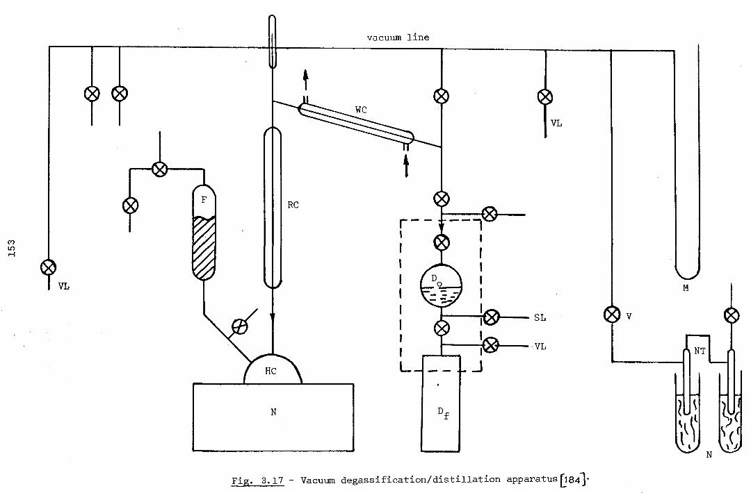
vacuum line

CO i n i

V

M

0

r n fS NT

I I I

N a

Fig. 3.17 - Vacuum degassification/distillation apparatus|j84)"

154

temperatures were computed and their mean was taken as the diffusion

tube temperature with an associated uncertainty of ±0.01°C.

The system was purged thoroughly by pumping the solvent through until a

steady baseline was observed on the chart recorder and the thermocouples'

readings indicated the isothermal condition. At this stage, valves

V^, and were the only ones open. Then Vp and the reference flow

control valve were shut, the pump was switched off and the gravity

flow control value was opened. The solvent feed from a well-stirred

and thermally-controlled reservoir (A) was then flowing through the dif-

fusion tube under gravity. Pumping of the fluid was avoided during

measurements since it imposes pulsations and disturbances upon the flow

which make the process experimentally complicated and theoretically dif-

ficult to handle {j66,J6 . Any change in the concentration, flow rate or the

temperature of.the flowing stream was observed by a change in the position

of the baseline on the chart recorder (Z) and by an offset of the zero

reading of the digital voltmeter (G). Flowrate measurements at the exit

of the diffusion tube ensured that the liquid was flowing through the

injection valve at constant velocity (Fig. 3.18). When the system was

under steady state condition, indicated by a steady baseline and zero

signal on the digital voltmeter, valves and were opened. The

solute from reservoir (B) identical to (A) was then flowing through the

sample loop, the injection valve being in the fill position (Fig. 3.3).

The DVM settings for the baseline zero output signal, the magnetic tape

recorder switch "on", the integration time (0.1 s), the time delay

(3.5 Ks) and the time intervals (5 s) were checked.

The solute was then injected into the flowing stream (i.e. by rotating

the injection valve shaft through 90°) and the time delay switch on the

DVM was set to the "on" position instantly. The solute flow control

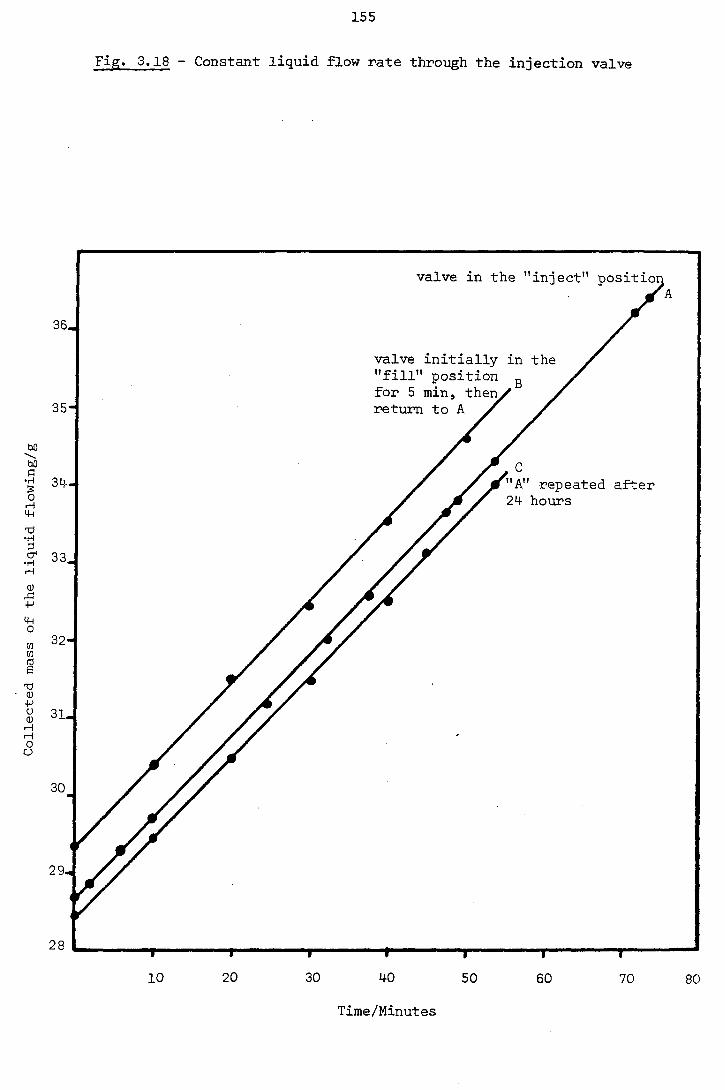
155

Fig. 3.18 - Constant liquid flow rate through the injection valve

36,

valve in the "inject" positior

valve initially in the "fill" position for 5 min, then^ return to A

"A" repeated after 24 hours

28 T —

10

—r-

20

T —

30 40

Time/Minutes

I

50 60 70 80

156

valve was closed and the thermocouples' readings were recorded.

The temperature of the diffusion tube was measured several times during

an experimental run which usually extended over a period of at least

one hour. The analog output signal of the differential refractoraeter

was digitized by the DVM and recorded on magnetic tape at five-second

intervals during the course of a single measurement. Each measurement

has been repeated at least three times. The recorded data were subse-

quently analysed to determine the moments of the effluent distribution

and hence the mean value of the diffusion coefficient.

3.10 Performance of the Equipment

3.10.1 Departures from the ideal model

The apparatus has been constructed according to the design specifications

resulting from the conclusions of the design study in Section 3.2.6.

Evidently, all the design criteria and constraints (Sections 3.2.2 -

3.2.6) are met so that the instrument does not depart from its ideal model

significantly. Computation of the effects of these departures shows that

some are negligible (i.e. less than ±0.04%) and others amount to no

more than ± 0.7%,

3 3 ^ 6 (y') ^ iS (a )

i.e. ^ ± 0.45% and " „ ^ ± 0.7%

Figure 3.19 contains the typical experimental results for hexane-heptane

mixtures at 45.8°C (pure hexane flowing). It shows the instrument's

working region where the effect of coiling the diffusion tube is neglig-

ible (less than 0.05%) for a dispersion time t > 3.3 Ks. The figure also

contains the prediction of equation (2.77) which has been calculated for

^c

our experimental arrangement, X = = 321.4, with the aid of the approp-

riate viscosity and density data [22,151,18^ and the measured diffusion

coefficient. The theoretical prediction is in good agreement with the

Deviation

,ob 1^2 -DI2\

j X 100%

I f ^ /

-5

Fig. 3.19 - Experimental determination of the coil effect

• - experimental data

- prediction by equation (2.77)

Working region

• # m ^

10

t, measurement time/Ks

158

experimental observation indicating that the effect of tube curvature is

negligible for t i 3.3 Ks. The experimental results contained in

Fig. 3.19 confirm the insignificance of coil effect by showing that the

observed diffusion coefficients are independent of the flow velocity to

within ±0.5% for such measurement times.

The agreement between the theoretical and experimental results, i.e.

Figs. 3.9 and 3.19, is remarkable particularly since no adjustable para-

meters have been used in comparison. We can therefore use the evident

agreement to support the use of Figs. 3.9 and 3.19 or equations (2.77-78) and

(2. 4-3 or 2.4-6) as a means of estimating the effect of tube curvature on our

measured diffusion coefficient. For the conditions employed in our

measurements, equations (2.77478) and (2.43 or 2.46) and Fig. 3.9 (workingregn)

2

revealed that even in the worst case (i.e. De .Sc = 18) for hexane-

octane mixtures around 70°C) the error incurred by the neglect of the

effects of tube coiling amounts to less than ±0.05%.

It must be pointed out that the mole fractions of the injection and

flowing stream did not differ by more than 0.1 throughout the measure-

ments. Consequently, errors due to composition and buoyancy effects

mentioned in the previous chapter were eliminated. Analysis of samples

of the solvent at the entrance and exit of the diffusion tube led to

the result of their compositions being identical, suggesting the

absence of any adsorption. The skewness and kurtosis of all eluted

peaks were found to be zero within the precision of the digital volt-

meter indicating that no perturbing effects arose from non-linearity of

the detector or adsorption of the injected species on the tube wall.

However, the adsorption of fully-saturated n-alkanes such as hexane,

heptane and octane (inert) on the stainless steel surface (inert) is

highly unlikely. From the experimental results of the"energetics of

159

adsorption of n-hexane and n-octane on. solid surfaces it can

be deduced that their adsorption on stainless steel is negligible.

3.10.2 Linearity of the detector

The determination of the diffusion coefficient from the characteristics

of the eluted distribution is dependent on the linearity of the response

of the refractive index detector. That is, the signal from the refracto-

meter should be directly proportional to the concentration difference of

the eluted species between the sample and reference sides of the cell.

In order to confirm this linearity for the present detector, measurements

of the zeroth moment (the peak area) for various known amounts of solute

injected, have been performed for the hexane-heptane mixture at 45.8°C.

Provided that the detector response is linear, the zeroth moment of the

eluted distribution should be directly proportional to the concentration

of the injected solute. Figure 3.20 shows the experimental results of

this test and indicates that only for large composition differences (i.e.

large refractive index n^ differences) between the injection sample and

flowing stream is the detector's response non-linear. This non-linearity

was expected due to the high sensitivity of the refractometer even at

- 8

extremely low composition differences (Gn^ g 10 ). Hence the samples

for injection were made such that they always differed in mole fraction

from the composition of the flowing stream by no more than 0.1 which is

well within the linearity range of the detector as shown by Fig. 3.20.

As mentioned earlier on, the skewness and kurtosis of all the eluted

peaks were found to be zero, confirming the detector's linear response

throughout this work.

3.10.3 The reference composition

Binary diffusion coefficients for the typical hexane-heptane mixture

(around 30°C) measured at various compositions of the flowing stream

and injection are included in Figs. 3.21 and 3.22. Also included in

160

these Figures are the reference compositions to which the measured

diffusivities should refer according to the theoretical analysis of

Chapter 2. Equation (3.8) was used to compute the reference composition

for a measured diffusion coefficient. The experimental and theoretical

results contained in Figs. 3.21 and 3.22 confirm the validity of

equations (2.180) and (3.8), showing that under the experimental con-

ditions employed throughout this work

°12 (*lr) = °12

where x^^ and x^^ are the reference and flowing stream mole fractions of

species 1 respectively.

3.10.4 Reproducibility of the results and precision

°12 -°12 Figure 3.23 plots — = , deviations of the measured diffusion coef-

Di2 ficients from their mean for the hexane-octane mixture f ~ O-G,

X, . = 0.7) at 50°C, against the measurement times t. It can be hex. 1

seen that for t ^ 3.5 Ks the results are reproducible to within ±0.45%.

Similarly for the mixture hexane-heptane (x^g^ ^ = 0.3, x^^^ ^ = 0.4)

at 27.8°C, the reproducibility of six repeated experimental runs each

taking around 4 Ks was found to be ±0.48% as shown by Fig. 3.24. The

deviations of the eluted distributions from normality under the conditions

of our experiments were insignificant as shown by Fig. 3.25, which is

typical for the hexane-heptane mixture.

It is not possible to perform the conventional analysis of random experi-

mental errors for these measurements to estimate their precision because

the diffusion coefficient is determined from the entire distribution

function of the eluted sample, and not a number of discrete measurements.

Consequently, the alternative strategy has been adopted whereby the

reproducibility of the measurements under nominally ,,identical thermo-

161

dynamic conditions is taken as a measure of the precision. On this

basis it is concluded that the precision of our experimental data is one

of ±0.5%. The graphical method proved to have an inferior precision

(2-5%) and hence it was discarded for the purpose of calculating the

results.

Furthermore, the diffusion coefficient for octane-dodecane mixture

^^oct f ~ I'O) at 24.95°C was measured and compared with its published

value [3^ determined at 25°C by the diaphragm cell method. It was found

-9 2 - 1 -9

that the two values, 1.699 x 10 (m s ) measured and 1.718 x 10 ± 1 %

(m^ s published, differed by only 1.0%.

The above results, together with the experimental results of the pro-

ceeding chapter, present a conclusive evidence for the correct operation

of our equipment.

3.10.5 Accuracy of the results

The largest single source of error in the measured diffusion coefficients

arises from the determination of the variance of the dispersion peak which

contributes an uncertainty of ±0.5%. The uncertainty in the determination

of the diffusion time and the possible systematic errors due to the cor-

rections discussed above amount to no more than ±0.2%. The only other

source of random error is the measurement of the tube radius and this

contributes ±0.24%. Thus the overall accuracy of the reported dissusion

coefficient values is believed to be ±1%.

Fig. 3.20 - Linearity of the refractometer

3.0

2 . 0 -

Zeroth moment

(arbitrary units)

1.0_

Working region

Pure hexane flowing.

Re = 3, t = 4 Ks

o> lO

'0.4 Tq. 6

^hep i' Mole fraction of injected heptane

3. 2X — Diffusion coefficient vs m o l e f r a c t i o n f o r h e x a n e — h e p t a n e m i x t u r e at 30 C

3. 88

3. 80

°12

(m^ s

3.70

3. 58

~ ^ 1 2 ± 0 . 1 %

cr> w

Mole fraction of heptane in the flowing stream,

Fig. 3.22 - Hexane-Heptane mixture at 29 C, xgf = 1 . 0

Measured diffusion coefficient vs mole

fraction of heptane injected.

+ expt Dl2(Xir) = * O'l'

^12^^1r^' eqns. (3.8) and (2.43)

3. 880

D X 10 12

3.837

-9

(m^ s ^) 3. 800

0

3.700

+ D ^ 12 +

*

T 0. 3% linear region J[

>

^ nonlinear N. region

1

cn •P

0. 8 1.0

x^., mole fraction of heptane injected

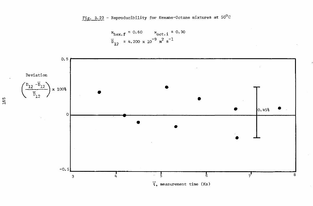
Fig. 3.23 - Reproducibility for Hexane-Octane mixtures at 50 C

*hex.f - O'GO *oct.i " —- —9 2 —* 1 D^2 = 4.200 x 10 m s

Deviation

^12 "^12 X 100%

12

0.45%

t, measurement time (Ks)

Fig. 3.24 - Reproducibility for hexane-heptane mixtures at 27. 8°C

t = * Ks; *hex.f = 0-3; *hex.l = O'"*

— — Q O — 1 D^2 = 3.553 X 10 m s

0. 5

UD H

"l? -»12

D 12

X 100% 0. M-8'6

Run No.

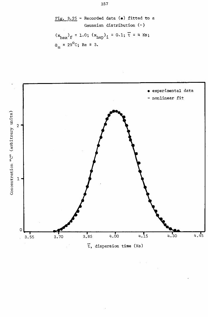
167

Fig. 3.25 - Recorded data (•) fitted to a

Gaussian distribution (-)

K e x ' f = '''hep'l = O'l; t = t Ife;

8^ = 29 C; Re = 3.

• experimental data

- nonlinear fit

m §

g •H

to

o

B •H % u §

I

H

3.70 3.85 4.00 4.15

t, dispersion time (Ks)

4.30 4.45

168

C H A P T E R 4

RESULTS

4 Introduction

The previous chapters have presented the theory behind the Taylor dis-

persion technique and described how the apparatus employed in this work

has been designed and used to perform accurate measurements of the liquid-

phase diffusion coefficients. Using this apparatus and the Taylor dis-

persion method, the binary diffusion coefficients for n-hexane-n-heptane,

n-hexane-n-octane and n-heptane-n-octane binary mixtures of various com-

positions were measured within the temperature range 20-70°C and at

atmospheric pressure. The time of measurements varied from about 4 Ks

to 8 Ks with the Reynolds Number for the flow being in the range 3 - 6.

In this chapter, we present the results of the measurements, with a repro-

ducibility of ±0.5% and an estimated overall accuracy of ±1%, and delay

the discussion and usage of these results until the next chapter.

The n-alkanes under investigation, n-C^H^^ (refractive index n^ = 1.3740 -

1.3760), n-C^H^g (n^ = 1.3880 - 1.3885) and n-CgH^g (n^ = 1.3970 - 1.3980),

were each at least 99.9% pure (see Chapter 3, Section 3.9). The stated

purity was supported by means of independent measurements of the refrac-

tive index of samples of the n-alkanes and through tests on a gas chroma-

tograph. The characteristics of the diffusion tube (Section 3.2.7) and

the method of evaluating the experimental results (Sections 3.5 - 3.8)

included in this chapter have been previously described in Chapter 3.

Tables 4.1 - 4.15 list the entire body of our experimental results for

the three n-alkane binary systems, each at five different compositions,

for a pressure of 1 bar (10^ Pa). Figures 4.1 - 4.15 display the binary

diffusion coefficient, as a function of temperature, 9^, at a constant

169

composition, for several mixtures.

For the purposes of correlating the experimental results and interpolating

the data within the range of measurements, the data were fitted to poly-

nomials, of the form Y = A^X^, by means of a least-squares comp"uter

program. As can be seen from Figs. 4.1 - 4.15 the data fitted the regres-

sion straight lines, of the form = A^ + A G , and the fitted

data agreed with the experimental ones with a maximum deviation of less

than 1%.

The values of constants A^ and A^ for the several mixtures of each binary

system are contained in Table 4.16 and the corresponding lines are disp-

layed by Figs. 4.16a - 4.16c. These Figures,which show the variation

of D^2 with 0^ along the constant composition lines, reveal that for each

binary system such lines are parallel, with a maximum slope deviation of

1% (typical of the C^-Cg system) according to the regression results

listed in Table 4.16.

In Figs. 4.17a - 4.17c the isotherms for the binary diffusion coefficient

as a function of composition, for each binary system, are shown. In

constructing these regression lines, of the form [Pjolg = A^ + A^x^^

k k . . with constants A^ and A^ being given for each case in Table 4.17, the

data has been employed at nominal temperatures computed from the earlier

regression results given in Table 4.16. The data fit these lines with

a maximum deviation of 0.5%.

All the isotherms of each binary system display similar behaviour and are

parallel with a maximum slope deviation of 3% (typical of the Cg-C^

and Cy-Cg systems). Thus variations of the binary diffusion coefficient,

with temperature and composition, within the range of measurements,

are linear to within a maximum deviation of 1% and 0.5% as shown by

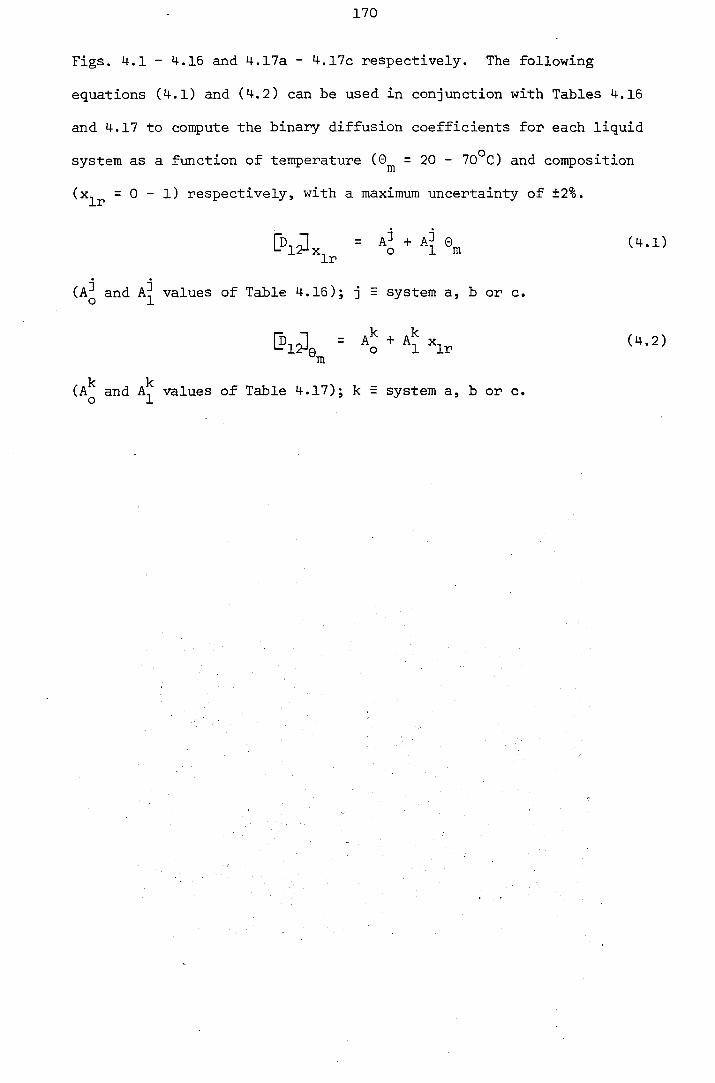
170

Figs. 4.1 - 4.16 and 4.17a - 4.17c respectively. The following

equations (4.1) and (4.2) can be used in conjunction with Tables 4.16

and 4.17 to compute the binary diffusion coefficients for each liquid

system as a function of temperature (8^ = 20 - 70°C) and composition

(x^p = 0 - 1 ) respectively, with a maximum uncertainty of ±2%.

[ j ' j K , = ''o + 4 Ir

(A^ and values of Table 4.16); j = system a, b or c.

B J a = Ao + *lr "••2)

k k (A^ and A^ values of Table 4.17); k = system a, b or c.

The binary diffusion coefficient, D22, as a function of temperature, 0^,

for the system hexane-heptane at fixed mole fractions of heptane, x^^,

and 1 bar pressure.

Table 4.1 e m

(°C) 2 9 (m^s X 10

26.375 3.7010

34.940 4.1180

42.751 4.5040

49.964 4.8500

50.989 4.9170

56.375 5.1710

D 12 9

(m^s X 10

5.0 -

4.0-

3.5.

3.0

Fig. 4.1

20

X, = 0.015 Ir

values obtained experimentally

values obtained by regression

T 30

T 40

T 50

T 60 70

Table 4.2

172

0m

(°C)

°12

(m^s~^) X 10^

27.388 3.6750

32.999 3.9370

40.375 4.3103

46.242 4.5950

55.762 5.0775

Fig. 4.2

°12

(m^s"^) X 10^

X. = 0.3015 Ir

• values obtained experimentally

values obtained by regression

5.0

4.5

4.0

3. 5

3.0

20 30 T 40 50

m

(°C)

T 60 70

173

Table 4.3

0 m

(°C)

^12

X 10^

28.661 3.6440

30.338 3.7560

34.485 3.9500

40.140 4.2165

45.638 4.4925

50.816 4.7530

58.000 5.0900

Fig. 4.3 = 0.4985

^12

(m^s X 10^

values obtained experimentally

values obtained by regression

5.0

4.5

4.0 -

3.5 -

3.0

20

1 —

30

-T"

40 m

(°C)

T "

50

1 —

60 70

174

Table 4.4

®Tn

(°C)

°12

X 10^

25.229 3.4475

36.239 3.9633

46.488 4.4445

54.116 4.8590

59.006 5.0635

Fig. 4.4 = 0.69 85

f 2 -1. 12 9 (m s ) X 10

• values obtained experimentally

values obtained by regression

5.0

4.5

4.0

3.5.

3.0 20 40

®m

(°C)

60 70

175

Table 4.5

e m Dl2

( ° c ) (m^s~^) X 10^

20 .010 3 .1010

29 .996 3 .5685

33 .253 3 .7360

39.068 4 .0050

41 .217 4 .1415

49 .630 4 .5500

54 .817 4 .8230

60 .008 5 .0515

Fig. 4.5 ^Ir - 0.9985

®12

X 10^

5.0 -

3.0 20

values obtained experimentally

values obtained by regression

I 30

—r-40

"T" 50

G 60 70

m

(°C)

176

The binary diffusion coefficient, 3_2' ^ function of temperature, G,

for the system hexane-octane at fixed mole fractions of octane,

and 1 bar pressure

Table 4.6 ( ° c ) 2 -1^2 9 (m s ) x 10

23.004 3.3035

29.853 3.6203

36.110 3.9137

43.968 4.2590

47.901 4.4816

54.000 4.7500

Fig. 4.8 ir 0 . 0 2 0 0

(nfs X 10^

4. 3

values obtained experi-. J mentally

values obtained by regression

3.8

3.3.

2 .8 .

2.3

20 I 30

T 40

(°C)

T 50 60 70

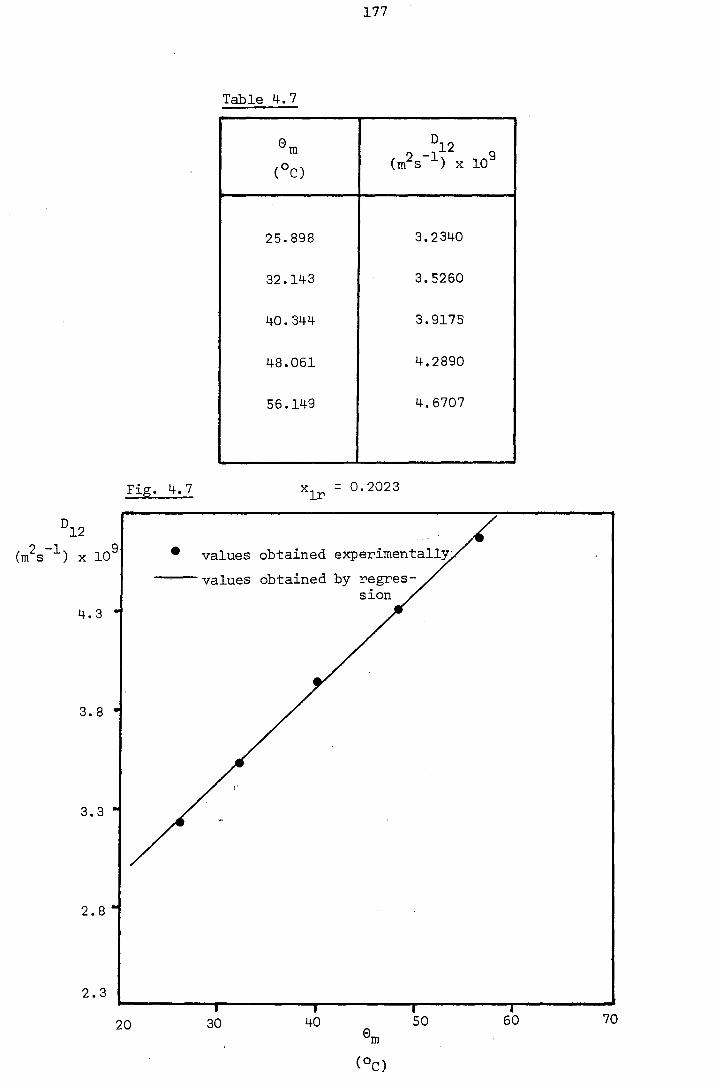
177

Table 4.7

Gm

( ° c ) 2 - I p 9

(mfs X 10^

25.898 3.2340

32.143 3.5260

40.344 3.9175

48.061 4.2890

56.149 4.6707

X = 0.2023

12

(m s X lO"

4.3

3.8 •

3.3

2 . 8

values obtained experimentalise

values obtained by regres-sion

2.3

20 — r 30

— r 40

%

(°C)

50 -T" 60 70

178

Table 4.8

(°c) 2 - i f 9 (m s ) x 10

25.888 2.9985

34.201 3.3740

41.673 3.7300

47.569 4.0000

54.139 4.3340

Fig. 4. X, = 0.4987 Ir

D 12

( m ^ s X 10"

• values obtained experimentally

values obtained by regression

4.3

3. 8

3. 3

2.8

2.3 20

T 30

T 40

m

(°C)

T 50

T 60 70

179

Table 4.9

(°C) 2 -lis 9

(m s X 10

23.001 2.6510

30.107 3.0010

41.619 3.5340

50.404 3.9300

60.299 4.4085

Fig. 4.9 X Ir

0.7038

2 9 (mis X 10

4. 3-

3. 8.

3.3.

2 . 8 -

values obtained experimentally

values obtained by regression

2.3 "I— 30 50

"T" 60 20

- r -40

m

(°C)

70

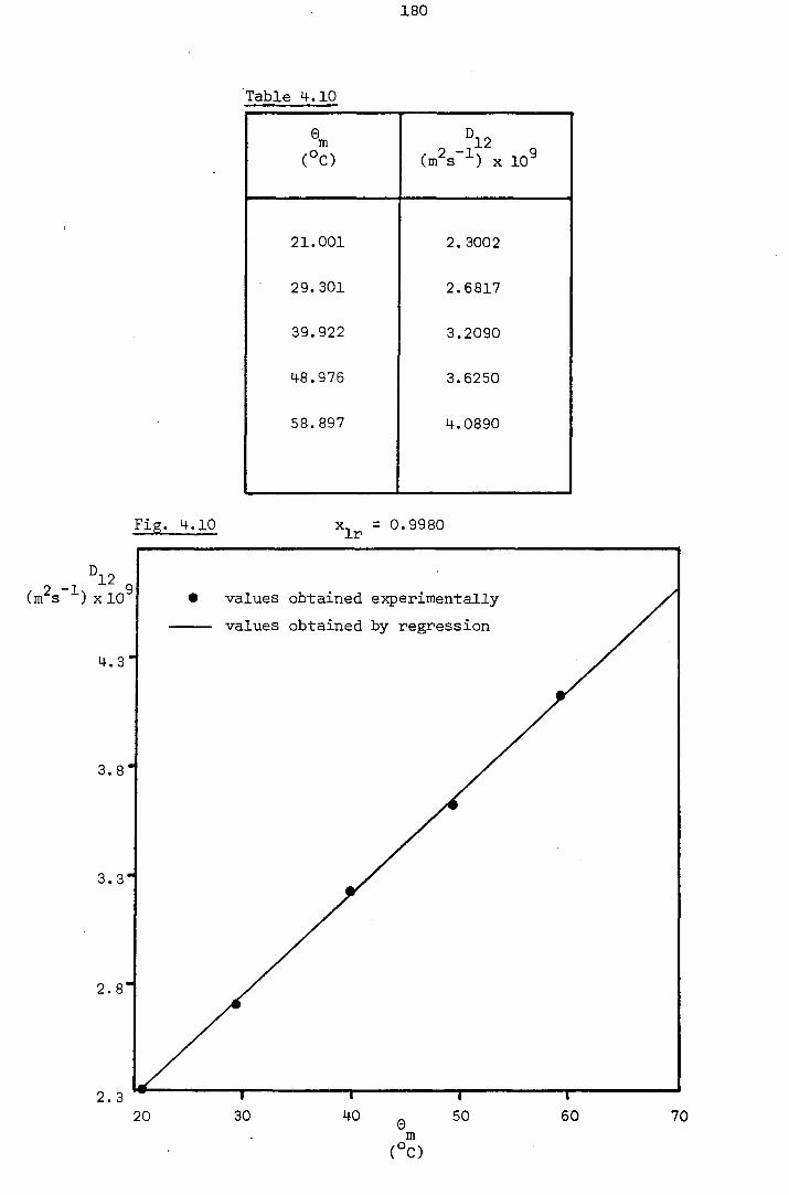
180

Table 4.10

®Tn ( ° c ) 2 - l " 9 (mi s •'•) X 10^

21.001 2.3002

29.301 2.6817

39.922 3.2090

48.975 3.6250

58.897 4.0890

Fig. 4.10 = 0.9980 Ir

2 - 1 9 (m s ) X 10

4.3

3.8

3.3'

2 . 8'

2.3

values obtained experimentally

values obtained by regression

1—

60 70

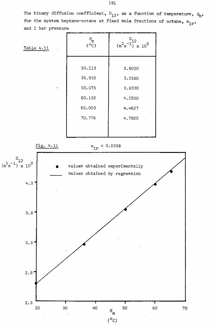
181

The binary diffusion coefficient, as a function of temperature,

for the system hep1

and 1 bar pressure

for the system heptane-octane at fixed mole fractions of octane,

, 2 -1^12 9 (m s ) X 10

4 . 3

3.8

3. 3

2 . 3

Table 4.11 (°c)

, 2 - ^ 2 9 (m s X 10

20.113 2.6020

35.932 3. 2580

- 50.075 3.8330

60.152 4.2500

65.003 4.4627

70.776 4.7820

Fig. 4.11 .0298

values obtained experimentally

values obtained by regression

20

I

30

—r-

40 - r 50

-T-

60 m

(°C)

70

182

Table 4.12

(°c) 2 - l " 9 (m s X 10

21.065 2.5490

32.211 3.0220

42.120 3.4100

59.371 4.1100

58.044 4.5220

Fig. 4.12

°12

X 10^

X = 0.2513

values obtained experimentally

values obtained by regression

4.3

3.8"

3 . 3

2.8'

2 . 3 20

T 30

T 40

m

(°C)

60 70

183

Table 4.13

0 m

(OC) 2 9 (m s X 10.

20.403 2.4361

35.029 3.0600

50.340 3.6565

59.615 4.0600

69.921 4.5369

Fig. 4.13 X, = 0.4988 Ir

2 -1 9 (m s X 10

4.3

3. 8

3. 3

2 . 8 ,

2.3

• values obtained experimentally

values obtained by regression

Table 4.14

184

Qm (°C)

^12 (m^s X 10^

22.489 2.4301

32.750 2.8560

46.047 3.4210

61.250 4.0400

68.752 4.3875

Fis. 4.14 ^Ir - 0.7488

2_-l 12

(m s ) X 10'

4.3

3. 8

3.3"

2 . 8

2. 3

values obtained experimentally

values obtained by regression

(°C)

Table 4.15

185

0 m

(°C) 2 -1^2 9 (in s • ) x 10

21.756 2.3125

29.548 2.6500

40.012 3.0930

53.128 3.6000

58.551 3.8320

63.644 4.0535

69.769 4.3622

Fig. 4.15 X = 0.9990

(mfs l)xlO^

4.3

3. 8

3. 3

2.8'

2.3

values obtained experimentally

values obtained by regression

60

(°C)

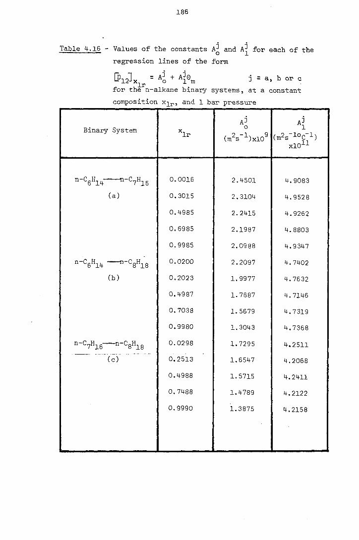
186

Table 4.16 - Values of the constants and for each of the

regression lines of the form

1 ^ 1 2 ^ = ^o + ^l®m j = a, b or c

for the n-alkane binary systems, at a constant

composition x^r, and 1 bar pressure

Binary System Xlr

A] o

(m^s~^)xl0^

4

(mfs-loc-l)

xlO^l

0.0016 2.4501 4.9083

(a) 0.3015 2.3104 4.9528

0.4985 2.2415 4.9262

0.6985 2.1987 4.8803

0.9985 2.0988 4.9347

""^6^14 ""^8^18 0.0200 2.2097 4.7402

(b) 0.2023 1.9977 4.7632

0.1+987 1.7687 4.7146

0.7038 1.5679 4.7319

0.9980 1.3043 4.7368

""^7^16 ^"^8^18 0.0298 1.7295 4.2511

(c) 0.2513 1.6547 4.2068

0.4988 1.5715 4.2411

0.7488 1.4789 4.2122

0.9990 1.3875 4.2158

187 _LO /

Fig. 16a - The binary diffusion coefficient, as a function

of teTrperature, 8^, for the system hexane-heptane at 5 different

mole fractions of heptane, and 1 bar pressure. 1 2 3 4 5

2 -1°^^ 9 (m s ) X 10

5.0

4.5

4.0-

3.5-

3.0

0016

4985

Fig. 16b - The binary diffusion coefficient, as a function

of temperature, 8 for the system hexane-octane at

5 different mole fractions of octane, at 1 bar

pressure

2 9 (m s X 10

4.3,

3.8,

3. 3.

2.8-

2 . 3

0200

9980

Gm (°C)

xoa

Fig. 16c - The binary diffusion coefficient, DQ_2j as a function of

temperature, G^, for the system heptane-octane at 5

different mole fractions of octane, and 1 bar pressure.

1 2 3 4

(m^s X icf

4.3

1: ^ir

0. 0298

2: ^ir = 0. 2513

3: ^ir

0. 4988

4: ^ir = 0. 7488

5: ^ r = 0. 999

3.8

3.3.

2 . 8 -

2 . 3

8 (°C) m

190

k k Table 4.17 - Values of the constants and A^ for each of the

regression isotherms of the form

t i j s = Ac + Xlr m

for the n-alkane binary systems at 1 bar pressure.

Binary System e m

(°c)

A^ •

(m^s"^) X 10^ (mfs'l) xl0^°

""^6^14 ""^7*16 20 3.3869 -3.0418

(a) 30 3.8804 -3.0614

40 4.3740 -3.0832

50 4.8676 -3.1057

60 5.3612 -3.1259

^"^6*14 ^"^8^18 20 3.1591 -9.1221

(b) 30 3.6337 -9.1388

40 4.1083 -9.1571

50 4.5828 -9.1738

60 5.0574 -9.1905

""^7^16 ^"^8^18 20 2.5906 -3.5838

(c) 30 3.0145 -3.6099

40 3.4383 -3.5356

50 3,8622 -3.6617

60 4.2861 -3.6878

70 4. 7100 -3.7150

Fig. 4.17a - Isotherms for the binary diffusion coefficient, D22, of hexane-heptane mixtures as a; function of heptane mole fraction, 1 ^ , at five different temperatures and 1 bar pressure.

2 - 1 ! " 9 (01 s • ) x 10^

5.0 _

4.5-

12

4.0-

D' 12

3.5-

D 12

3.0

values obtained experimentally

values obtained by regression

40°C

30°C

20°C

0 . 2 0.4 0.6 0. 8 1.0 X Ir

Fig. 4.17b - Isotherms for the binary diffusion coefficient, DJ_2j of hexane-octane mixtures as a function of octane mole fraction, x^^, at five different temperatures and 1 bar pressure.

2 -1\^^ 9 (mis - ) X 10* A values obtained experimentally

values obtained by regression

5,0 D 12

60^

4.0 -50"C

40°^

30^

3.0 12

2 0 ° C '

2.0

0.2 0.4 0.6 0. 8 1.0

Ir

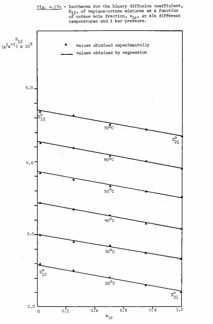
Fig. 4.17c - Isotherms for the binary diffusion coefficient, ^12» heptane-octane mixtures as a function of octane mole fraction, at six different temperatures and 1 bar pressure.

2 9 (m s ) X 10 ^ values obtained experimentally

values obtained by regression

5.0 -

_D 12

4.0'

12

2.0

70°C

50°C

50°C

40°C

30°C

20°C

0 0.'4 0.6 O!8 1.0

X Ir

195

C H A P T E R

DISCUSSION

5. Introduction

The present experimental data may be used for three purposes. First,

the measurements stand alone as definitive values for binary (or mutual)

diffusion coefficients for the three systems: n-hexane + n-heptane,

n-hexane + n-octane, and n-heptane + n-octane. Secondly, they can be

employed to assess the validity of the theoretical descriptions of dif-

fusion processes in liquid mixtures such as those discussed in Chapter 1.

Finally, they provide a test of the various empirical prediction schemes

for liquid-phase diffusion coefficients. In this Chapter, we consider

the last two of these uses in some detail.

5.1 Data for the properties of the pure components and their mixtures

In order to proceed with the above investigations, further relatively

accurate data (around ±1%) for the n-alkane mixtures, for example, density,

molecular size parameters, viscosity and other properties, are required.

Surprisingly, such data for the relatively simple liquid mixtures studied

here, particularly in the temperature and composition ranges needed,

were difficult to find and in many cases unobtainable. However, with

the aid of several publications [6, 39, 113, 151, 187, 188^ and insti-

tutions [22 , 177]] we have managed to gather the accurate data (±3% maximum)

for the pure components contained in Tables 5.1 and 5.2.

The densities of the mixtures were evaluated using equation (3.7) whilst

the corresponding kinematic viscosities were obtained by analogy with the

diffusivity results of Chapter 4, That is, from Figs. 4.17(a)-(c), a

196

TABLE 5.1 - Properties of the pure components [6, 18"^

Component Molecular Weight

M

Critical Volume"

/ V (ml)

Normal Boiling Point, T]3

(OK)

A A

xioi«

(m)

n-Hexane 86.178 370 341.9 5.77 (a)

n-Heptane 100.205 432 371.6 6.05 (b)

n-Octane 114.232 492 398.8 6.28

TABLE 5 AAA

.2

6

(°C) ' hex

(C.P)

' hep (C.P.)

^oct (C.P.)

' hex (g/ml)

^hep (g/ml)

' oct (g/ml)

20

(a) 0.312 0.414 0.549 0.659 0.684 0.703

30 0.282 0.371 0,486 0.650 0.675 0.695

40 0.254 0.336 0.434 0.641 0.666 0.687

50 0.234 0.304 0.390 0.631 0.658 0.678

60

(b) 0.215 0.267 0.333 0.622 0.649 0.671

70 0.187 0.231 0.284 0.613 0.641 0.663

•k • , • . 1. Ql+S Molar volume at = 0.28 (V^) [6]

Mean molecular diameters (a) 20-60°C; (b) 20-70°C [iS"^

Data accurate to (a) ±1%; (b) ±3% [22, 177^

1 9 7

correlation for the present experimental diffusion coefficients (equation

(4.2)) may be written in the form

1^12^ 8 " *1^21 ^2^12 (5.1)

which is identical to the empirical equation (1.52). Here,

D°^ = Lim D 2 ; D° = Lim D (5.2)

. Xg-K) x ^ ^

Thus, by analogy with equation (5.1), the kinematic viscosity, v, is

obtained from the equation

~ ' l l •*" =2^2 (5.3)

Since v = n/p, where n and p denote the dynamic viscosity and density

respectively, from equations (3.7) and (5.3) and Tables 5.1 and 5.2 it is

possible to write a correlating equation for the composition dependence

of the dynamic viscosity in the form

^12^8 ~ ^1^ 1 ^ ^2^ 2 (5.4-)

which reproduces the available experimental data with a maximum deviation

of ±0.5%.. Finally, it is useful to record that the absolute viscosity

data contained in Table 5.2 fitted the regression lines

^hex ~ 0. 355 8 - 2.m x 10 ^8 for pure n-hexane (5.5)

(8 = 20 - 50°C) ; in m Pa-s

^hept ~ 0.4845 - 3.662 x 10 ^8 for pure n-heptane (5.6)

(8 = 20 - 70°C)

-3 and ^oct ~ (0.6495 - 5.279 x 10 8 for pure n-octane (5.7)

(8 = 20 - 70°C)

with a maximum deviation of ±2.5%. These equations are similar to our

198

general empirical equation (H-.l) which gives the variation of the binary

diffusion coefficients with temperature, G, in the range 20 - 70°C.

5.2 The molecular dynamics approach to the interpretation of binary diffusion coefficients in n-alkanes

The molecular dynamics simulation based on the rough hard sphere theory

(Sections 1.2.3 and 1.3.4), formerly developed by Chandler and

Dymond [j8, 8 ^ for pure fluids, has been extended by Czworniak, Anderson

and Pecora [87 and Bertucci _et al. [ 8]] and employed to investigate the

composition dependence of the binary diffusion coefficients of several

two-component solutions. They arrived at the conclusion that for ideal

solutions (e.g. binary solutions of n-alkanes, or benzene, chlorobenzene,

bromobenzene and toluene), the calculated diffusion coefficients were

in 'excellent' agreement (with a mean deviation of ±1% to ±6%) with

experiment. But the recent results of Castro and Calado [^9, 18' ] indicate

that this is only true for self-diffusion coefficients and binary diffusion

coefficients of n-alkanes of close carbon numbers. Nevertheless, we now

employ the theoretical analysis described by Czworniak [sf] in

order to predict the temperature and composition dependence of the binary

diffusion coefficients for the n-alkane mixtures studied here and compare

the results with those of the present work.

The kinetic diffusion coefficient, based on the theory of irrever-

sible thermodynamics and discussed in Chapter 1, Section 1.2.3. is,

under isothermal and isobaric conditions, given by

„expt

where is the experimental binary diffusion coefficient and 6^ is

the non-ideality thermodynamic factor

9 Jin a.

^ ^ ^ 9 £n X .

199

For the present systems [39, 14^ the factor may be expressed as

= 1 + 0.002(n^ - ^2)^X2*2 '

so that for the present purposes, it may be taken as unity with negli-

gible error. Czwomiak et [ST] and Bertucci et [sCI assume

that 0^2^ of a real binary fluid is equal to that of a two-component

mixture of rough hard spheres at the same temperature and with the same

number density and mole fraction as the real fluid, the masses of hard

spheres being equal to those of the corresponding molecules. In this

case, the theoretical, or kinetic, binary diffusion coefficient is given

by equation (1.71) which may be rewritten as

^

k 1 Ti The Enskog kinetic diffusivity, at an absolute temperature T, is

obtainable from

pkin \ CT ' / 1 \

A . where n is the total number density, defined by

N p

(5.10)

so that n^ = n x^ (5.12)

O1+O2 and 0^2 - — 0 — particle (or molecular) size parameter (5.13)

23 -1 N = 6.022 X 10 mole (Avagadro's number)

K = 1.381 X 10 J °K ^ (Boltzman's constant)

If the last bracket term of equation (5.10) is excluded, the equation

becomes identical to that for a dilute, binary gas mixture. In addition.

200

and nig represent the molecular masses of the diffusing species and

®12^'^l2^ the pair distribution function for unlike species at contact.

The factor F accounts for the deviations of the diffusion coefficient

from the Enskog value arising from molecular velocity correlations.

The symbol A represents translational-rotational coupling constant

introduced by Chandler which is supposed to depend just upon the

molecular species involved and is, in particular, independent of compo-

sition and temperature.

In the present analysis, we presume that equation (5.9) is valid and

have employed our experimental data to determine the translational-

rotational coupling constant A for each system at two representative

temperatures 20°C and 70°C. For this purpose, we have calculated the

pair distribution function 522^"^12^ according to the method proposed by

Czworniak ^ [ST] . In their approach the pair distribution function

is written as

= gpy<''l2>[?cs - " J

where Spy('^22 the Percus-Yevick pair distribution function for

unlike hard spheres. In addition, is the Percus-Yevick [isf] com-

pressivity factor and that for the Carnahan-Starling [ss]] equation

of state for hard-sphere systems. All of the quantities Spys and

Zpy may be expressed as analytic functions of the packing fractions of

individual species, in a hard-sphere mixture,

• i =

and the total packing fraction

<l> = + *2 (5.15b)

201

The factor F, which expresses the- deviations of the diffusion coefficient

of a real hard-sphere fluid mixture from that of an Enskog fluid, has been

obtained from a correlation of the results of molecular dynamics simu-

lations of self-diffusion in fluid mixtures [79, 8" . The simulations

were carried out for a trace of one species in another and for mass

and size ratios near unity, and so yield the factor F at limiting con-

centrations F(<j), m^/mg, 1) or F(^, m^/mg, a^/a2, 0). Czwomiak

et al. [sv] have suggested that the value of F appropriate to any mixture

of the same two components may be obtained by a simple linear combination

of these results so that

F($, m^/mg, = x^F(0, m^/mg,, 1)

+ XgFC*, m^/mg, G^/Og, 0) (5.16)

The correlations for F(^, m^/mg, o^/Og, 0) have been adapted here with-

out change.

In order to make use of these results we have employed the rigid sphere

diameters of the n-hexane, n-heptane and n-octane determined by Castro

and Calado which permit the evaluation of §22(^12^ and F for each

binary system at each temperature. Subsequently, the value of the tran-

slation-rotation coupling constant A for each system has been determined

by a least-square fit to the present experimental data for each tempera-

ture. It should be noted that the determination of A in this manner does

not affect the composition dependence of the diffusion coefficient obtai-

ned theoretically, but merely serves to scale the results.

Figures 5.1 - 5.3 contain plots of the experimental diffusion coefficients

together with the least squares representation of them according to

equations (5.9) and (5.10). Table 5.1 includes the values of the rigid

202

FIG. 5.1 - Binary diffusion coefficient, D12, of the hexane-heptane mixture as a function of composition, at 20°C and 50°C and 1 bar, determined experimentally and by Molecular Dynamics Simulation

X 10

n-CgH^^+n-CyH^c at 60 C

0.978

4.5

4.0 _

3.5 _

3 . 0

=

6.05 X 10 1° m - 1 0

5.77 X 10 m

values obtained experimentally

( i.e.

•values obtained by M.D. computer simulations

(i.e. D theory 12

)

i A = 0.930

m

max

^1 = Or, =

1%

= 2.5%

6.05 x 10~^° m

5.77 X 10~^° m

at 20°C

0 . 2 0.4 0.6 0 . 8 1.0 Mole Fraction of Heptane xj_

2Ub

FIG- 5.2 - Binary diffusion coefficient, D12, of the heptane-octane mixture as a function of composition, at 20°C and 70°C and 1 bar, determined experimentally and by Molecular Dynamics Simulation

D^2 X 10

(m^ s-1)

4.8-

4.4 -

4.0

3.6 —

3.2 -

2 . 8 -

2.4 -

2.0

values obtained experimentally

(i.e.

values obtained by M.D. computer simulation

(i.e. Dthsory)

n-C^H^g + n-CgH^g at 70^C

0.911

o. =

— 1 Q 6.28 X 10 m

-10 6.05 X 10 m

5%J

A =

^m =

\ = max cr, =

=

0.876

2%

2.5% -10

6.28 X 10 m - 1 0

6.05 X 10 m

n-CyH^g + CgH^g at 20°C

I I I 0,2 0.4 0.6

Mole Fraction of Octane 0.8

FIG. 5.3 - Binary diffusion coefficient, DJ_2J of the hexane-octane mixture as a function of compo-sition, at 20°C and 60°C and 1 bar, determined experimentally and by Molecular Dynamics Simulation

4.8

4.4'

4.0'

3.6'

3.2"

2.8"

2.4-

2.0

A = 0.797

A = m

max = 7%

values obtained experimentally

( i.e.

values obtained by M.D. computer simu-lation

theory (i.e. D 12

)

"'^6^14 + n-CgH^g at 60 C

—10 a, = 6.28 X 10 m

-10 02 = 5.77 X 10 m

A = 0.733

A =1.7% m

- 2%

10%

n-CgH^^ + n-CgH^g at 20 C

0.2 0.4 0.6

Mole Fraction of Octane x^

0.8 1.0

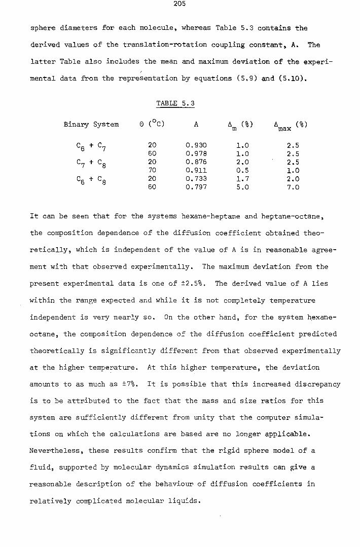
20 0.930 1.0 2.5 60 0.978 1.0 2.5 20 0.876 2.0 2.5 70 0.911 0.5 1.0 20 0.733 1.7 2.0 60 0.797 5.0 7.0

205

sphere diameters for each molecule, whereas Table 5.3 contains the

derived values of the translation-rotation coupling constant, A. The

latter Table also includes the mean and maximum deviation of the experi-

mental data from the representation by equations (5.9) and (5.10).

TABLE 5.3

Binary System 0(°C) A A ( % ) A (%)

in IT18X

Cg +

+ Cg S ^8

It can be seen that for the systems hexane-heptane and heptane-octane,

the composition dependence of the diffusion coefficient obtained theo-

retically, which is independent of the value of A is in reasonable agree-

ment with that observed experimentally. The maximum deviation from the

present experimental data is one of ±2.5%. The derived value of A lies

within the range expected and while it is not completely temperature

independent is very nearly so. On the other hand, for the system hexane-

octane, the composition dependence of the diffusion coefficient predicted

theoretically is significantly different from that observed experimentally

at the higher temperature. At this higher temperature, the deviation

amounts to as much as ±7%. It is possible that this increased discrepancy

is to be attributed to the fact that the mass and size ratios for this

system are sufficiently different from unity that the computer simula-

tions on which the calculations are based are no longer applicable.

Nevertheless, these results confirm that the rigid sphere model of a

fluid, supported by molecular dynamics simulation results can give a

reasonable description of the behaviour of diffusion coefficients in

relatively complicated molecular liquids.

206

5.3 Validity of simple models of diffusion

The simple models of diffusion discussed in Chapter 1, Section 1.2,

such as Eyring's activation energy [63, 65j and Stokes-Einstein models

[l3, 17, 12"^ suggest that the group [KT/D^^n] should be temperature

independent. Thus the applicability of such models may be assessed by

an examination of the constancy of the experimental values of the group

[kT/D°2il] for the liquids investigated in this work. Accordingly,

Fig. 5.4 displays plots of this group as a function of absolute tempera-

ture, which have been constructed with the aid of our diffusivity data

for the extremely dilute solutions (i.e. the limiting values) and

the viscosities contained in Table 5.2. It is evident that the group

[KT/D^^n] increases as the temperature is increased beyond 313 °K. In

particular, for the hexane-heptane system, the value of the group at 333 °K

lies some 8% above that at 293 °K, whereas for the heptane-octane system

the discrepancy at 343 °K is 12%. Thus, on this basis, and because the

mixtures considered here are very nearly ideal, we must conclude that

neither the Eyring nor the Stokes-Einstein model, or other similar models,

are entirely adequate to describe the diffusion processes in liquids.

5.4 Schemes for predicting the liquid-phase diffusivities

There exist a large number of empirical prediction and correlation schemes

for the binary diffusion coefficient in liquid mixtures, relying to a

varying extent on simplified theories (Chapter 1). Because it is impos-

sible to carry out measurements on all possible systems over a wide range

of conditions, it is certain that such schemes will continue to be used

for engineering design purposes for some time to come. Now we employ the

present experimental data in order to assess the validity of some of the

prediction schemes in frequent use.

207

FIG. 5.4 - The group [KT/D^gn] for two n-alkane binary

systems at infinite dilution

p ^ 1 X 10-

4 . 0 -

3.8 —

3.6 —

3 •

3.2.

3.0

n-heptane + n-octane

*hept ^

n-heptane + n-hexane

Xhept 1

293 303 313 323

4%

333 343

T (°K)

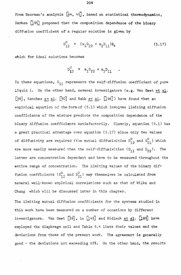
208

From Bearman's analysis [44, M-s]], based on statistical thermodynamics.

Darken [l9^ proposed that the composition dependence of the binary

diffusion coefficient of a regular solution is given by

°12 ~ (xi°22 ^2°ll^^t (5.17)

which for ideal solutions becomes

°12 ~ *1°22 ^2^11

In these equations, represents the self-diffusion coefficient of pure

liquid i. On the other hand, several investigators (e.g. Van Geet et al.

[39] , Sanchez ejt [so] and Babb _et [196] ) have found that an

empirical equation of the form of (5.1) which involves limiting diffusion

coefficients of the mixture predicts the composition dependence of the

binary diffusion coefficients satisfactorily. Clearly, equation (5.1) has

a great practical advantage over equation (5.17) since only two values

of diffusivity are required (the mutual diffusivities 0°^ and 0°^) which

are more easily measured than the self-diffusivities (D^^ and Dgg)- The

latter are concentration dependent and have to be measured throughout the

entire range of concentration.. The limiting values of the binary dif-

fusion coefficients (D°2 ^21^ may themselves be calculated from

several well-known empirical correlations such as that of Wilke and

Chang which will be discussed later in this chapter..

The limiting mutual diffusion coefficients for the systems studied in

this work have been measured on a number of occasions by different

investigators. Van Geet [39], Lo [l45]] and Bidlack £t 0-8^ have

employed the diaphragm cell and Table 5.4- lists their values and the

deviations from those of the present work. The agreement is generally

good - the deviations not exceeding ±2%. On the other hand, the results

209

of Moore and Wellek [iSOj obtained with a porous frit apparatus deviate

considerably from the present data as shown in Table 5.4 and Figs. 5.5 .

and 5.6. In the worst case, the deviation amounts to 11%. These devia-

tions, com lined with the non-physical behaviour displayed by Moore and

Wellek's results confirm that the porous frits method of measurement is

not reliable [3' .

A semi-empirical expression for the composition dependence of the binary

diffusion coefficients of ideal liquid mixtures has been deduced by

Hartley and Crank [l8, 27, 5^ which may be written as

KT

= c + mx (Bearman [l8, 2l\)

where is a constant proportional to the molecular diameter, a^, of the

diffusing species. It is useful to note that at either end of composition

range x^ = 0-1, this equation reduces to the familiar Stokes-Einstein

relation (Chapter 1).

The present data for the diffusion coefficients, together with the avail-

able viscosity data (Table 5.2 and equation (5.4)) may be employed to

test the applicability of this relationship. Figure 5.7 contains a plot

of the group [^22^12^'^ as a function of the mole fraction for the

hexane-heptane system at three temperatures - which is linear as expected

on the basis of equation (5.18). This linearity allows us to determine

the values of and from the intercept and slope of the line.

Assuming that ot' = ira , the values of (for n-heptane) and (for

-10

n-hexane) derived were = (6.07, 6.10 and 6.30) x 10 m and (5.95,

5.88 and 6.10) x 10 m for T = 293, 313 and 333 °K respectively. The

mean values for each species are therefore = 6.16 x 10 m and

210

- 1 0

Og = 5.97 X 10 m which are in quite good accord with those obtained

in other ways (Table 5.1).

For the remaining systems. Fig. 5.8 shows that equation (5.18) is not

obeyed, which casts considerable doubt on the general validity of equation

(5.18).

Finally, Tables 5.4 and 5.5 compare the present results with those

obtained from several commonly used correlations for predicting the

limiting diffusivities of binary liquid mixtures. In particular, we

include the Wilke-Chang equation [l90] which requires the viscosity of

the solvent and the molar volume of the solute (V^)^ at the normal

boiling point of the solvent. It can be seen that this correlation leads

to deviations of as much as 14% from the present results. It has been

found that a modest improvement in the predictions of this scheme may

be achieved if (V^)^ is replaced by (V^)^, the molar volume of the

solute at the temperature at which the diffusion coefficient is to be

calculated (see Tables 5,4 and 5.5).

The other methods of prediction which have been examined include those

due to Lusis-Ratcliff [l9ij, Otherm-Thakar [l9^ , Scheibel [s] and

Reddy-Doraiswamy [l94]. Table 5.4 demonstrates that among these, only

the Lusis-Ratcliff method leads to generally good results. Over the

entire body of the present experimental data only the modified Wilke-

Change method or the Lusis-Ratcliff scheme provide acceptable predictions

of the diffusion coefficients with a maximum deviation of ±6% (Tables

5.4 and 5.5).

Thus, in conclusion, three important facts have emerged as a result of the

data presented in Chapter 4. First, the simple models describing dif-

fusion in liquid mixtures on the basis of Stokes-Einstein's or Eyring's

211

treatment are generally inaccurate. Secondly, the interpretation of

temperature and concentration dependence of the binary diffusion coef-

ficients by the rough hard-sphere model is in excellent agreement with

our experimental results for n-hexane t n-heptane, and n-heptane +

n-octane mixtures, but for the n-hexane + n-octane mixture the agreement

deteriorates. This suggests that only for the binary mixtures in which

molecular mass ratios of the diffusing species are close to unity is

the present scheme appropriate. Finally, we have found that the con-

centration dependence of the binary diffusion coefficients of the n-alkanes

studied here is given very accurately (±2%) by the empirical correlation

1^21^0 " *1°21 ^2° 12

TABLE 5.4 - Comparison of the literature values of the limiting diffusion coefficient D°2 with those obtained in this work, for three different binary mixtures at 25°C and 1 bar.

Solute 1

Solvent 2

< 2

( M ^ S X 1 0 ^

Data Reference % Deviation From Present

Work

n-C^H^g 3.71 (l) Present work 0 n-C^H^g

3.75

3 . 7 8

3 . 2 7

3.74

3.63

(2) Lo 1145] (Diaphragm cell)

(3) Bidlack et al. [IsgJ (Diaphragm cell (4) Wilke-Chang |l9^ (original; at (5) Wilke-Chang (modified in this

work; at (VJL)Q) (6) Lusis-Ratcliff

[191] (7) Othmer-Thakar

[192] (8) Scheibel [l9^

-1

-2

12

-1

2

3.64

(2) Lo 1145] (Diaphragm cell)

(3) Bidlack et al. [IsgJ (Diaphragm cell (4) Wilke-Chang |l9^ (original; at (5) Wilke-Chang (modified in this

work; at (VJL)Q) (6) Lusis-Ratcliff

[191] (7) Othmer-Thakar

[192] (8) Scheibel [l9^

2

3.58

(2) Lo 1145] (Diaphragm cell)

(3) Bidlack et al. [IsgJ (Diaphragm cell (4) Wilke-Chang |l9^ (original; at (5) Wilke-Chang (modified in this

work; at (VJL)Q) (6) Lusis-Ratcliff

[191] (7) Othmer-Thakar

[192] (8) Scheibel [l9^ 3.5

3 . 3 2 (9) Reddy-Doraiswamy [194]

10

N - C G H ^ G " - 2 6 * 1 4

3.46

3,46

(1)

( 2 )

0

0

3.47 (3) -0.3

2 . 9 8 (4) 14

3 . 2 5 (5) 6

3 . 3 2 ( 6 ) 4

3.56 (7) -3

3.34 ( 8 ) 3.5

3.17 ( 9 ) 8

N - C S H L B n-C^H^g 2.85

2.84

(1)

(2)

0

0.3

2. 88 (3) -1

2.45 (4) 14

2.70 (5) 5

2.70 (6) 5

2.26 (7) 2 0

3.16 ( 8 ) -10

2.61 (9) 8

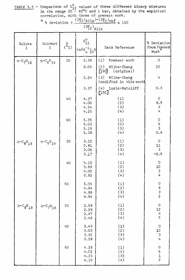
TABLE 5.5 - Comparison of values of three different binary mixtures in the range 20 - 50°C and 1 bar, obtained by the empirical correlation, with those of present work.

(D22)Aliz)-(D22)ref deviation X 100

^^12^Aliz

Solute 1

Solvent 2

0 ( ° C )

"12 Data Reference

% Deviation From Fr^sert Work '

n C^H^g 20

40

60

n CgH^g 20

40

60

n C^H^g 20

40

60

3 . 3 8

3 . 0 5

3.24

3.37

(1) Present work

(2) Wilke-Chang [l9( (original)

(3) Wilke-Chang (modified in this work)

(4) Lusis-Ratcliff [191]

4.37 (1) 4.00 (2) 4.24 ( 3 )

4.25 (4)

5.35 (1) 5.03 (2) 5.19 (3) 5 . 3 8 (4)

3.15 (1) 2.81 (2) 3.06 (3) 3.17 (4)

4.10 (1) 3.69 (2) 4.00 (3) 3 . 9 2 (4)

5.05 (1) 4.64 (2) 4.88 (3) 4.94 (4)

2.58 (1) 2.28 (2) 2.47 (3) 2.45 (4)

3.43 (1) 3.03 (2) 3 . 3 2 (3) 3 . 2 8 (4)

4.28 (1) 4 . 0 2 (2) 4,23 (3) 4.19 (4)

0

10

0.3

0

8.5 3 4

0 6 3

0.6

0 11 3

-0.6

0 10 2

4

3 2

0 12 4 5

0 12 '3 4

0 6 1 2

Fin. 5.5 - Comparison of the limiting diffusion coefficients for the heptane-octane mixtures at different temperatures and 1 bar, obtained by Moore and Wellek |1.5l], with those determined in the present work. .o D 12

3.0

2 . 8

2 . 6

2.4 -

2 . 2

Lim (D.g) ' *1 heptane mole fraction

values obtained in this work

values obtained by Moore & Wellek Eisi]

0 (°C)

FIG. 5.6 - Percentage deviation of the values obtained by Moore and Wellek, (0°2^MW those obtained in this work, (^i2^Alis

10-

% deviation

5"

-5"

-15

© ©

© ©

^°12^Aliz"^°12W ..

'•°l2^Aliz

20 25 30 G (OC)

"i+T

ZJ.0

FIG. 5.7 - Stokes-Einstin group, ' for the hexane-heptane mixture at 1 bar, against heptane mole fraction x.

T - 1 N °K xlO^ 4; 25

4.15_

4.05.

3.95-

3.85-

3.75-

3.65-

3.55-

3.45'

FIG. 5.8 - Stokes-Einstein group, [Pi2 12' ' for hexane-octane

and heptane-octane binary mixtures at 293 °K and 333 °K and 1 bar, against octane mole fraction x .

L T J

N °K~^ X 10 ^ 5

4.1 -

4.0 -

3.9 -

3.8 -

3.7 -

3.6 -

3.5 -

3.4 -

3.3

Calculated values for:

217

C O N C L U S I O N S

The work described in this thesis has demonstrated that the Taylor

Dispersion Technique has now been developed to a point where it permits

accurate measurements of diffusion coefficients of liquid mixtures over

a moderate range of temperatures. Because the technique is rapid and

simple it is now possible to use the technique to accumulate a large body

of data on a wide variety of well-chosen systems in the same temperature

range. The technique also lends itself to operation at elevated pres-

sures and over a wider range of temperatures. It is therefore suggested that

these are two directions for future work.

The experimental data obtained in this work are of sufficient accuracy

that they provide a stringent test of available molecular theories and

prediction procedures. Although none of the theories examined is capable

of describing the experimental data within their uncertainty, the

rough hard-sphere theory which makes use of molecular dynamics simulation

results is the most promising. Nevertheless, it seems that molecular

dynamics simulation of diffusion for molecular models more similar to

the alkanes such as spherocylinders would be useful.

218

R E F E R E N C E S

[1] (a) R.K. Ghai, H. Ertl and F.A.L. Dullien, AIChE J. 3^, 881

(1973); 20 , 1 (1974).

(b) I.R. McDonald and J.P. Hansen, "Theory of Simple Liquids",

Academic Press, 1976.

(c) J.A. Pryde, "The Liquid State", Hutchinson Pub., 1966.

(d) H.N.V. Temperley and D.H. Trevena, "Liquids and Their Proper-

ties", Ellis Harwood, 1978.

(e) J.O. Hirschfelder, C.F. Curtiss and R.B. Bird, "Molecular

Theory of Gases and Liquids", John Wiley & Sons, N.Y., 1954.

[2] S.A. Rice and J.P. Boon, "Comments on the experimental and theoreti-

cal study of transport properties in simple liquids", a review

prepared exclusively for the Chemistry Department of ISM of Chicago

University, Chicago, Illinois (1980).

U.S. Department of Commerce and National Bureau of Standards, "The

Technological Importance of Accurate Thermophysical Property Infor-

mation", N.B.S. Special Publication No. 590, Washington (Oct. 1980).

[4] M. Assael, C.A. Nieto de Castro and W.A. Wakeham, Proc. of Chempor 78,

Braga, Portugal, 1978.

[53 E.G. Scheibel, J. Ind. Eng. Chem. No. 8, 1569 (1954)*

[X] R.C. Reid, T.K. Sherwood and J.M. Prausznitz, "The Properties of

Gases and Liquids", 3rd ed., McGraw Hill, 435-469, 566-601.(1977^'

[73 D.M. Himmelblau, Chem. Rev. 527 (1964).

[sj J.F. Davidson and E.J. Cullen, Trans. Inst. Chem. Engrs. J_5, 51 (1957),

219

[g] A. Alizadeh, C.A. Nieto de Castro and W.A. Wakeham, 3rd Nat.

Meeting on Chemistry, Portugal, Centro de Quimica Estrutural, IST,

Lisbon, 1980.

[10] J.W. Williams and L.C. Cady, Chem. Rev. 1^, 171 (1934).

[11] (a) L.G. Longsworth, Annals. New York Acad. Sci. 46, 211; (b) L.

Onsager, 241 (1945).

[123 (a) E.A. Mason and T.R, Merrero, "Advances in Atomic and Molecular

Physics", Bates and Eastermann Eds., 155, Academic Press, N.Y.,

1970; (b) J. Phys. Chem. Ref. Data 1 , 3 (1972).

[1^ (a) H.J.V. Tyrrell, "Diffusion and Heat Flow in Liquids", Butter-

worth, London, 1961; (b) "Diffusion Processes", J.N. Sherwood et al.,

eds., 1 , Ch. 2, Gordon and Breach, N.Y., 1971.

[143 R.F. Treyball, "Mass Transfer Operations", 2nd ed., McGraw-Hill, 1968,

[153 (a) J.M. Thomas and W.J. Thomas, "Principles of Heterogeneous

Catalysis", Academic Press, 1967; (b) J.J. Carberry, "Chemical

Catalytic Reaction" _9, McGraw-Hill, 1976.

[163 H.J.V. Tyrrell and M. Mitchell, J. Chem. Soc. Faraday Trans. II,

358 (1971).

[l"^ R.B. Bird, W.E. Stewart andE.N. Lightfoot, "Transport Phenomena",

Wiley Intn. Ed., Chs. 16-19, 1960.

(j. K.C. Pratt and W.A. Wakeham, Proc. Roy. Soc. Lond. A336, 393 (1974).

A.C. Ouano, Ind. Eng. Fun dam. IJ., No. 2, 268 (1972).

[20] A.C. Ouano and J.A. Crothers, J. Phys. Chem. _7§.J No. 13, 1314 (1975).

220

[2]J A. Alizadeh, C.A. Nieto de Castro and W.A. Wakeham, Int. J.

Thermophys. 243 (1980).

[2; Amer. Petrol. Inst. Petrol. Refin. Tech. Data Book Nos. A4220-B4220

(1964-72); National Engineering Laboratory, Glasgow - private com-

munication through Dr. Isdale.

[23 (a) K.C. Pratt and W.A. Wakeham, Proc. Roy. Soc. Lond. A3M-2, 401

(1975); (b) J. Chem. Soc. Faraday Trans. II, 7^, 977 (1977).

[243 H.J.V. Tyrrell and P.J. Watkiss, Ann. Rep. Chem. Soc. A 35 (1976).

[2^ E.R. Pike, "Photon Correlation Light Beating Spectroscopy". H.Z.

Cummins and E.R. Pike, eds., NATO Adv. Study Institute Series,

Plenum, London, 5 (1974).

[26] H.J.V. Tyrrell and A.W. Ellis, Symp. on Transport Props. Fluids,

N.E.L., Glasgow, April 1979.

[2" (a) W.A. Wakeham and D.H. Slater, J. Phys. B: Atom. Mol. Phys. 6_,

886 (1973); (b) ibid. 1_, 297 (1974).

[28]] Confidential Report on "The Chloride Ion Diffusivities", prepared

at Imperial College by W.A. Wakeham ^ for the ICI Mond Division

(1979).

[2^ B. Anderson and T. Berglin, Proc. Roy. Soc. Lond. A377, 251 (1981).

]3o] V. Hancil, V. Rod and M. Rosenbaum, Chem. Eng. Commun. _3, 155 (1979).

[siTl K.G. Denbigh, "The Principles of Chemical Equilibrium", 2nd ed.,

Cambridge University Press, 86 (1968).

I3C! T.E. Gruz, "Transport Phenomena in Aqueous Solutions", Ch. 3, Adam

Hilger , 1974.

221

[33] H.J.V. Tyrrell, J. Chem. Educ. 41, 397 (1964).

[34] A. Pick, Pogg. Annalen _94, 59 (1855).

J. Crank, "The Mathematics of Diffsuion", 2nd ed. Oxford Univer-

sity Press, 1975.

[36j J.G. Kirkwood, P.J. Dunlop, R.L. Bladwin, L.J. Costing and G. Kegeles,

J. Chem. Phys. 1505 (1960).

[37] P.J. Dunlop, B.J. Steel and J.E. Lane, "Physical Methods of Chemistry",

A. Weissberger and B.W. Rossiter, ed., _1, Part IV, 205, Interscience,

1972".

[3CI P.J" Dunlop, K.R. Harris and C.K.N. Pua, J. Phys. Chem. _74, 3518 (1970),

[3CI A.L. Van Geet and A.W. Adamson, J. Phys. Chem. 68_, 238 (1964); A.L.

Van Geet, PhD Thesis, University of Southern California, Los

Angeles, 1961.

M M.J. Pikal, J. Phys. Chem. 76, 3038 (1972).

[41] A. Gassman and J. Sedlacek, Z. Phys. Chem. 240, 26 (1969).

[4^ P.J. Dunlop and I.R. Shankland, J. Phys. Chem. _7§.> 1319 (1975).

[4^ (a) S.R. de Groot, "The Thermodynamics of Irreversible Processes",

Amsterdam, 1963; (b) I. Prigogine, "Introduction to the Thermodynamics

of Irreversible Processes", Oxford University Press, 1968.

[44] T. Loflin and E. McLaughlin, J. Phys. Chem. _73, 186 (1969).

[4^ R.J. Bearman and J.G. Kirkwood, J. Chem. Phys. 2^, 136 (1958).

[4^ A.S, Cukrowsky and B. Baranowski, Z. Phys. Chem. 240, 167, 253 (1969).

222

S.A. Rice and P. Gray, "The Statistical Mechanics of Simple

II Liquids, Interscience, N.Y., 1965.

J.H. Dymond and T.A. Brawn, Sump, on Transp. Props. Fluids, No. 3.4,

N.E.L., Glasgow, 1979.

(49] W. Southerland, Phil. Mag. 9_, 781 (1905).

[50J A. Einstein, Ann. Phys. 1^, 289 (1906);^, 591 (1911).

[51I F. Perrin, J. Phys. Radium, _7, 1 (1936).

[5^ R.O. Herzog, R. Illig and H. Kudar, Z. Phys. Chem. 167, 329 (1933).

13C] R.J. Bearman, J. Chem. Phys. _32, 1308 (1960).

[51 P. Walden, Z. Electrokem. ]^, 77 (1906).

[5^ L.G. Longsworth, J. Amer. Chem. Soc. _7 , 5705 (1953).

[jeJ A. Poison, J. Phys. Chem. 649 (1950).

[57] A.R. Gordon, J. Chem. Phys. _5, 522 (1937).

[5 1 J.H. Wang, J. Phys. Chem. 686 (1954).

[59] G.S. Hartley and J. Crank, Trans. Faraday Soc. 4^, 801 (1949).

[6Q] C. Carman and L.S. Stein, Trans. Faraday Soc. 619 (1956).

[enT] H.S. Hamed, Disc. Faraday Soc. 2^, 7 (1957).

[eCl C.J. King and C.H. Byers, J. Phys. Chem. _70, 2499 (1966).

[53] H. Eyring, S. Glasstone and K.J. Laidler, "The Theory of Rate

Processes", McGraw-Hill, 1941.

223

[64] H. Eyring, J.F. Kincaid and A.E. Steam, Chem. Rev. 28, 301 (1941).

[es] J. Frenkel, "Kinetic Theory of Liquids", Dover, N.Y., 1955.

[663 T. Einwohner and B.J. Alder, J. Chem. Phys. 49, 1458 (1968).

[67] S. Nir and W.D. Stein, J. Chem. Phys. 55, 1958 (1971).

[es] J. Hirschfelder and H. Eyring, J. Phys. Chem. 41, 249 (1937).

[e^ J.C.M. Li and P. Chang, J. Chem. Phys. 23, 518 (1955).

[70l I. Ruff and V. Friedrich, J. Phys. Chem. 25, 3297 (1971).

[71] G.M. Panchenkov, Zh. Fiz. Khim. _24, 1390 (1950).

[72] D. Frenkel, G.H. Wegdam and J. Van der Elsken, J. Chem. Phys. 57,

2691 (1972).

[73Q S.J.K. Jensen, D. Kivelson and M.K. Ahn, J. Phys. Chem. 2940

(1972).

[71 J.H. Dymond and B.J. Alder, J. Chem. Phys. 2061 (1966).

[7^ D. Tabor, "Gases, Liquids and Solids", Penguin, 1970.

[7^ P.C. Hemmer, M. Kac and G.E. Uhlenbeck, J. Math. Phys. 60 (1964),

[jt] E.B. Smith and B.J. Alder, J. Chem. Phys. 1190 (1959).

[7^ J.H. Dymond, Physica 75, 100 (1974).

[7^ B.J. Alder, D.M. Gass and T.E. Wainwright, J. Chem. Phys. 5_3, 3813

(1970).

[8(^ S. Chapman and T.G. Cowling, "The Mathematical Theory of Non-

Uniform Gases", Camb. Univ. Press, 1939.

224

[s] B.J. Alder, "Prediction of Transport Properties of Dense Gases and

Liquids", UCRL 14891 T, Univ. Calif. Berkeley, U.S.A. (1966).

[823 B.J. Alder and J.H. Dymond, "Van der Waals' Theory of Transport in

Dense Fluids", UCRL 14870 T, Univ. Calif. Berkeley, U.S.A. (1966).

[83j (a) J.H. Dymond, J. Chem. Soc. Faraday Trans. II, 1789 (1972);

(b) J. Chem. Phys. 969 (1974); (c) 1J_, 101, 175 (1976);

(d) Proc. 6th Symp. Therraophys. Props. ASME 143, New York (1973).

[84] J.H. Dymond and T. Brown, Proc. 7th Symp. Thermophys. Props. ASME

660, New York, (1977).

[ss]] N.F. Camahan and K.E. Starling, J. Chem. Phys. 51 , 635 (1969).

[sCI (a) D. Chandler, J. Chem. Phys. 3500, 3508 (1974); (b) 62,

1358 (1975).

[373 K.J. Czwomiak, H.C. Anderson and R. Pecora, Chem. Phys. 11, 451

(1975).

[s^ J.J. Bertucci and W.H. Flygare, J. Chem. Phys. _63, 1 (1975).

C.A. Nieto de Castro and J.C.G. Calado, Chem. Soc. Symp. Transport

Props. Polyatom. Fluids, Statistical Mechanics & Thermodynamics

Group, Imperial College, London (April 1980).

[9( V. Sanchez and M. Clifton, Ind. Eng. Chem. Fundam. 2^, 318 (1977).

[9]] S.A. Rice and P. Gray, "The Statistical Mechanics of Simple Liquids",

Interscience, N.Y., 1965.

0 ^ (a) P. Gray; (b) B.J. Alder and W.G. Hoover; (c) W.W. Wood,

"Physics of Simple Liquids", H.N.V. Temperley, J.8.. Rowlinson and

G.S. Rushbrook eds.. North Holland, Amsterdam, 1968.

225

S.A. Rice, J.P. Boon and H.T. Davis, "Simple Dense Fluids",

Academic Press, N.Y., 1968.

[g'i] G.H.A. Cole, "The Statistical Theory of Simple Dense Fluids",

Pergamon Press, Oxford, 1967.

£9^ J. Jeans, "An Introduction to the Kinetic Theory of Gases", Camb.

Univ. Press, 1967.

{9^ F.C. Collins and M. Raffel, J. Chem. Phys. 2_9, 699 (1958).

[973 B.J. Alder and T.E. Wainwright, Phys. Rev. Lett. 18, 988 (1967).

[9^ B.J. Alder, AIP Conf. Proc. n , 1 (1973).

[9^ W.A. Steel, "Transport Phenomena in Fluids", Marcel Dekker, N.Y.,

1969.

[lO(£l B.J. Alder and T.E. Wainwright, "Transport Processes in Statistical

Mechanics", Interscience, 1958.

[lO]] (a) W.W. Wood and J.E. Erpenbeck; (b) J.R. Dorfman et al.,

"Statistical Mechanics" B: Time Dependent Processes (Plenum, N.Y.,

1977).

{10^ W.G. Hoover and M. Ross, Contemp. Phys. 3^, 339 (1971).

[103] W.W. Wood and F.R. Park,er J. Chem. Phys. 27 , 720 (1957).

[104] B.J. Alder and T. Einwohner, J. Chem. Phys. 43, 3399 (1965).

[10^ S.A. Rice and A.R. Allnatt, J. Chem. Phys. 409 (1961).

[10^ G.L. Gouy, Compt. Rend. Acad. Sci. Paris 90, 307 (1880).

226

[lO'fJ L.G. Longsworth, J. Amer. Chem. Soc. 2516 (194-7).

[lO^ G. Kegeles and L.J. Costing, J. Amer. Chem. Soc. 2516 (1947).

Q.0^ L.J. Costing,, E.M. Hanson, C. Kegeles and M.S. Morris, Rev. Sci.

Instr. 20, 209 (1949).

[ll(^ L.J. Costing and M.S. Morris, J. Amer. Chem. Soc. _71, 1998 (1949)

[lliQ L.J, Costing and L. Onsager, J. Amer. Chem. Soc. J74, 6066 (1952).

Q-l^ L.J. Costing and H. Fugita, J. Amer. Chem. Soc. 79_, 1359 (1957).

[lis] J.C. Shieh and P.A. Lyons, J. PHys. Chem. _73, 3258 (1969).

[llf] H.J.V. Tyrrell and C.J. Dudley, J. Chem. Soc. Faraday Trans. I.

6^, 2200 (1973).

|3lC] T.A. Renner and P.A. Lyons, J. Phys. Chem. 2_8, 2050 (1974).

[llf] J.M. Creeth, J. Amer. Chem. Soc. 77, 6428 (1955).

[ll'3 A.L. Babb, J.R. Hall and C.S. Caldwell, Rev. Sci. Instr. 28_, 816

(1957).

]%1^ L.J. Costing and H. Kim al. , Rev. Sci. Instr. 1602 (1973).

[ll^ (a) 0. Bryngdahl, Acta. Chemica. Scand. 3J., 1017 (1957); (b)

U , 684 (1958).

{l2(^ T.C. Amu, Doctoral Thesis, Faculty of Science, Upsala Univ.

Sweden, 1978.

|12]2 J.C. Albright and D.C. Miller, J. Phys. Chem. 26, 1853 (1972).

[l2^ K.W. Beach, R.H. Muller and C.W. Tobias, Rev. Sci. Instr. 40,

1248 (1969).

227

^ 2 ^ F.R. McLarnon, R.H. Muller and C.W. Tobias, Applied Optics 14,

2468 (1975).

[l2^ D. Gabor, Proc. Roy. Soc. A197, 545 (1949).

[l2^ L.O. SundelBf, Arkiv f8r Kemi 2_5, 1 (1965); idem. Chem. Scripta.

6, 55 (1974).

[12^ J.N. Northrop and M.L. Anson, J. Gen. Physiol. 543 (1928).

[127] R.H. Stokes, J. Amer. Chem. Soc. 72, 763, 2243 (1950).

[12^ R. Mills and L.A. Woolf, "The Diaphragm Cell", Austral. Nat. Univ.

Press, Canberra, 1968.

[120 H.J.V. Tyrrell and G.J. Dudley, J. Chem. Soc. Faraday Trans. I 69,

2188 (1973).

[l3(^ G. Wedlake and F.A.L. Dullien, J. Chem. Eng. Data 19, 230 (1974).

[131] C. Bamas, J. Appl. Phys. _5, 4 (1934).

[1323 A.R. Gordon, Ann. N.Y. Acad. Sci. 285 (1945).

[133] J.B. Lewiss, J. Appl, Chem. 228 (1955).

[134] R.D. Walker, K.E. Gubbins and R.N. Bhatia, Trans. Faraday Soc.

2091 (1968).

[l3^ W.H. Hayduk and S.I. Oakimidis, J. Chem. Eng. Data 21, 255 (1976).

jl36] J.T. Holms. Rev. Sci. Instr. 36, 831 (1965); Holms al•j J.

Phys. Chem. £7, 1409 (1963).

[137] J.O.L. Wendt and G.C. Fraizer, Ind. Eng. Fundam. 12, 239 (1973).

228

[l38] M.T.- lyn and W.F. Calus, J. Chem. Eng. Data 2^, 310 (1975).

[iS^I C.J.D. Fell and H.P. Hutchinson, Ind. Eng. Chem. Fundam. 10,

303 (1971).

[l4(^ R.W. Laity and M.P. Miller, J. Phys. Chem. 68, 2145 (1964).

[l4iQ A.F. Collings, D.C. Hall, R. Mills and L.A. Woolf, J. Phys. E.

425 (1971).

[142] R.R. Irani and A.W. Adamson, J. Phys. Chem. 62 , 1517 (1958).

[143] R.L. Robinson, W.C. Edmister and F.A.L. Dullein, J. Phys. Chem.

258 (1965).

[144] S.A. Sanni, C.J.D. Fell and H.P. Hutchinson, J. Chem. Eng. Data

13, 424 (1971).

[14^ H.Y. Lo, J. Chem. Eng. Data 1^, 236 (1974).

Q.4^ H.S. Carslaw and J.C. Jaeger, "Conduction of Heat in Solids", 2nd

edn., Oxford Univ. Press, 1959; J. Crank, "The Mathematics of

Diffusion", 2nd edn., Oxford Univ. Press, 1975.

[14'^ (a) H.S. Hamed and D.F. French, Ann. N.Y. Acad. Sci. 267 (1945);

(b) H.S. Harned and R.M. Hudson, J. Amer. Chem. Soc. _7 , 5880 (1951).

[14^ G.I. Taylor, Proc. Roy. Soc. London A219, 186 (1953); A223, 446;

A225, 473 (1954).

[l4^ A.R. Aris, Proc. Roy. Soc. London A235, 67 (1956);*F.R. Tillman,

PhD Thesis, Texas University, U.S.A., _9, 108 (1966).

[l5(^ W.A. Wakeham and C.A. Nieto de Castro, Symp. 2nd Encontro Nat. de

Quimica OPORTO, Portugal, January 1979.

229

|j 5l] J.W. Moore and R.M. Wellek, J. Chem. Eng. Data 19, 136 (1974).

[iS:^ D.W. McCall and D.C. Douglass, J. Phys. Chem. 71, 987 (1967).

[l53] K.J. Packer, C. Rees and D.J. Tomlinson, Mol. Phys. ]^, 421 (1970);

R.J. Hyward and K.J. Packer, ibid. 23, 1083 (1972); ibid. 26,

1533 (1973).

[l5i£j T. Uano and T. Aratani, Seigyo Kogaku, ]^, 18 (1968).

[l55|] 0. Levenspiel and K.B. Bischoff, Adv. Chem. Eng. J4, 105 (1963);

0. Levenspiel and W.K. Smith, Chem. Eng. Sci. _6, 227 (1957).

1^56^ C.Y. Wen and L.T. Fan, "Models for Flow Systems and Chemical

Reactors", Marcel Dekker, N.Y., 1975).

[isf) S. Goldstein, "Modem Developments in Fluids Dynamics" 313,

Dover, N.Y., 1965.

[j.5^ M.E. Erdogan and P.C. Chatwin, J. Fluid Mech. _2£, 465 (1967).

[l5^ D.J. McConalogue, Proc. Roy. Soc. London A315, 99 (1970).

[l6^ R.J. Nunge, T.S. Lin and W.N. Gill, J. Fluid Mech. 363 (1972).

[l6l] L.A.M. Janssen, Chem. Eng. Sci. Jl, 215 (1976).

Il62] W.R. Dean, Phil. Mag. 5, 673 (1928).

[led H.C. Topakoglue, J. Math. Mech. 1^, 1321 (1969).

[164] D.J. McConalogue and R.S. Srivastava, Proc. Roy. Soc. London

A307, 37 (1968).

[165] J.S. Ultman and H.S. Blatman, AIChE J 2^, 169 (1977).

2 3 0

[l6^ R.N. Trivedi and K. Vasudeva, Chem. Eng. Sci. 2j9: 2291 (1974).

[iS"^ K.D.P. Nigam and K. Vasudeva, Chem. Eng. Sci. 835 (1976).

[l6^ E. Th. Van der Laan, Chem. Eng. Sci. _7, 187 (1958).

{l6^ H. Schlichting, "Boundary Layer Theory", 6th edn., McGraw-Hill,

N.Y., 1968.

[l7C^ C.B. Thorsness, PhD Thesis, Illinois University, Urbana, USA, 1975.

[l7jQ M.R. Hopkins, Proc. Phys. Soc. _M, 703 (1938).

[17^ N.G. Barton, J. Fluid Mech. 74, 81 96 (1976);.

[173] R. Smith, J. Fluid Mech. 88, 323 (1978).

[174] R.D. Patel, J.J. McFeeley and K.R. Jolls, AIChE J. 21, 259 (1975);

B.N. Wood, A.W. Seed and M.R. Nerem, J. Fluid Mech. 52, 137 (1972).

[l75|] J.M. Kay, "An Introduction to Heat Transfer", 2nd edn., 6.2, 66,

Cambridge Univ. Press, 1968.

Q.7^ D.L. Bidlack and D.K. Anderson, J. Phys. Chem. 6_8, 206, 3790 (1964).

[l7^ Engineering and Science Data Unit London - Private communication and

item no. 79027, viscosity (alkanes).

[l7^ P. Eisenklam and L.F. Flint, Cand. J. Chem. Eng. J£7, 101 (1969).

[l7^ P. Eisenklam and L.F. Flint, Proc. Roy. Soc. London A315, 519

(1970); "Oil Recovery", Private communication with Dr. P.

Eisenklam, Chem. Eng. Dept., Imperial College, London.

[l8(^ Amer. Inst. Phys., "Temperature and Its Measurements in Science

and Industry", 199 (1945).

2 3 1

[isi] International Practical Temperature Scale of 1976, N.P.L., Revised

edn., H.M.S.O., London (1976).

[l8^ M. Assael, PhD Thesis, Imperial College, London, (1980).

[isf] B.D.H. Chemicals Laboratory (Middx), Private communication.

[l8'+] C.A. Nieto de Castro, PhD Thesis, Institute Superior Tecnico,

Lisboa (1977).

[isCl H.C. Van Ness and M.M. Abbott, Ind. Eng. Chem. Fundam. 17, 66 (1978).

[l86] A.V. Kiselev, Q. Rev. XV. 99 (1961).

J.C.J. Calado and C.A. Nieto de Castro, J. Chem. Soc. Faraday

Trans, (to be published).

[i88] E.L. Heric and J.G. Brewer, J. Chem. Eng. Data 574 (1967).

[l8^ D.L. Bidlack, T.K. Kett, C.M. Kelly and D.K. Anderson, J. Chem.

Eng. Data 1^, 342 (1969).

[l9^ C.R. Wilke and P. Chang, AIChE J. 1, 264 (1955).

[l.9l] M.A. Lusis and G.A. Ratcliff, Can. J. Chem. Eng. 40, 385 (1968).

0^92] P.P. Othmer and M.S. Thakar, Ind. Eng. Chem. 589 (1953).

[193] E.G. Scheibel, Ind. Eng. Chem. _W, 2007 (1954).

[I9I£| K . A . Reddy and L . K . Doraiswamy, Ind. Eng. Chem. Fun dam. 7 7 ( 1 9 6 7 ) .

[19^ L.S. Darken, Trans. Amer. Inst. Mining Met. Eng. 175, 184 (1948).

[l9^ A.L. Babb and C.S. Caldwell, J. Phys. Chem. 6£, 51 (1956).

[19"^ G.A. Mansoori, N.F. Camahan, K.E. Starling and T.W. Leland, Jr.,

J. Chem. Phys. 54, 1523 (1971).

232

L I S T O F S Y M B O L S

A Translational-rotational coupling constant

A Cross-sectional area of the diffusion tube 0

A Elliptical cross-section area A®, A^ Constants (n = 0, 1, 2 ... , m = i, j, k ...)

A Effective cross-sectional area of the pores P

a^, ^2 Major and minor axes of the elliptical cross-section of the non-uniform tube

a^ The activity of species i

a' Cell thickness

B , B™ Constants (n = 0, 1, 2 ... , m = i, j, k ...)

c . 3 in B^ The thermodynamic factor for solute 1 = 1 + ^ ^

, rpv n 2mn" 3 ^ b The co-volume = — r — a d p

b' The optical lever arm for the convergent light in the diffusiometer

C, C° Fluid concentrations, in general and (molar) in the uniform tube respectively

C°, C° C^j C^ Top and bottom cells concentrations at times zero and 1 D , i D , . _

t respectively

^If ""li' ""Ir Molar concentrations of species i in the flowing and injection streams and that of the reference respectively

C^, ]_m' ^1 Perturbation to the flowing stream composition, its mean and that of the uniform tube

AC^ Average concentration perturbation

AC, Perturbation to the concentration in the detector d

6C^ Correction to the flowing stream concentration

C-, Cp, C„ Recorded concentrations (end and beginning) n -tj -ti

c, c^, c^ Molar concentrations in general^ that of species i and the total respectively

c' Perturbation to the concentration distribution

*

Concentration of the labelled species i

Cp The p"*" spatial moments of the concentration distribution (p = 0-4)

233

Diffusivities of species i in general and based on volume frame of reference respectively.

D..J D.., D? Binary-, self-, and Tracer-Diffusion coefficients of the ^species (i = integer, j = integer; i ?! j)

D, D"*", D^, Dg, D^, D^g Diffusion coefficients, general, hard-sphere fluid, dense gas, due to Dymond and Enskog at high and low densi-ties and that calculated by molecular dynamics simulations respec-tively

D^2 Concentration dependent binary diffusion coefficient

D°2 5 The limiting values of D^^ at and Xg ^ 0 respectively

D(t), D Integral diffusion coefficient and its average respectively

^12' ^12 Binary diffusivitiesof a coiled and elliptical cross-section tube respectively

D^2 Binary diffusion coefficient at the flowing stream composition tubes respectively

^12' ^^12^p Concentration and density dependent binary diffusivities,

^SH' Diffusivities derived by the smooth-, and rough-hard sphere models respectively

^12^' Kinetic binary diffusiviity and thatof Enskog respectively

^12^^' ^12^theory Experimental (= D^^ values in Chapter 4- Tables)

and theoretical binary diffusion coefficients °12

Activity dependent binary diffusion coefficient = /dZnx

R ^ c

d Diameter of the liquid reservoir

De Dean' s number = Re. (rg—) ' K

C

E or En, E Effective diffusivities of the diffusion J and ^r^u^ \ ^ """IZ

. RoUo")

V

connecting — j tubes respectively

E° E at the flowing stream composition

e Eccentricity Q (l-(-g^)^)^

F Correction due to the correlated motion of the particles

f^ N -particle distribution function P P

fg, fy Effective friction coefficients for the Brownian and the hard-sphere motions respectively

fg, Frictional force of resistance of each spherical and non- • spherical solute molecule

fg Empirical values of f^

234

gCOp) The radial distribution function at contact for two like spheres

^12 (^12^ The radial distribution function at contact for two unlike" spheres

H(s) Transfer function

AH The latent heat of evaporation evap

h The driving head for the liquid flow

6h Change in h

j\ Molar flux of species i with respect to stationary coordinates

relative to molar average velocity

m' " h Mass and heat fluxes in general

jY Jj, with respect to the volume frame of reference

J Bessel function - zeroth order of the first kind o

T- Mass fluxes of species i relative to stationary or moving coordinates respectively

j Total number of fringes

K Boltzmann's constant = 1.381 x 10 J °K ^ ,

Constant = 2.1701 ... x 10 ^ (eqn. (2.23))

Ky Kliprtosis = ( — ) - 3 a

k: , k^ Rate constants for the backward and forward reactions respectively

k^ Number of any fringe maximum

L Length of the diffusion tube

6L Small length of the tube A

Phenomenological coefficients

5*: A A • L , L,, L. corresponding to the effects of Vy and V9J on mass and heat mm' nh ^ i

transport of species i respectively

A A L , L, The cross coefficients, i.e. effects of Vy and 38: on heat and mh' hm ^

mass transport respectively

i Length of the connecting tube

a Distances - axial (optics) and vertical (diaphragm cell) respectively

M^ Molecular weight of species i

CWJ Mobility - velocity gradient as a result of unit force

235

Mass of a sphere or particle (molecular atom) i (i = integer)

m Reduced mass =

m^ Cross-section averaged c^

23 -1 N Avagadro's number = 6.022 x 10 (mol )

Molar flux of species i relative to the mass average velocity

Number of moles of species- i (in the injection) in excess of those having an equal volume in the flowing stream

N. Number of moles of species i in phase 6 ip

dN^g Number of moles of species i leaving phase B

Np Number of particles (atoms, spheres, molecules, etc.)

n, n^ Number of molecules, and that of species i

n^, n^^ Refractive index, and that of species i

n" Number density of a fluid system (pure or binary mixture)

5*C , A n^ Number density of the n-alkane i = n

n^ Number density for a dilute gas

^ir Mass flux of species i relative to the mass average velocity

P, p Pressures - in general and that of the fluids in the tube

Pe Peclet number ''12

AP Pressure drop across the diffusion tube

Q Volumetric flowrate

Qg Quantity defined by equation (2.135); f(Pe, Sc)

Q Reduced height-area ratio • ~ 1 O " 1

R The universal gas constant = 8.314 J mol K

R Internal radius of the diffusion tube o

R Coil radius c

R(z) Internal radius of the non-unifOrm tube 2R U

Re Reynolds number = — - —

Rg(S2), R^(U) Resistances of the iron-cons tantan therraoc cuples (latter = 2§.7507f2)

r^ Internal radius of the connecting tube

236

T Radial distance (polar coordinate)

r^, r^^ Radii of spheres and particles i

Sc Schmidt number = ~ — 12

Entropy of the system i A ^3 T" 3

Sk Skewness of the eluted distribution = —r or U p

s Laplace transform variable

T Absolute temperature

T^, Boiling and critical temperatures respectively

t Time in general

t Measurement time = o

tg Taylor-Aris minimum time criterion

t , tJ Correction times contributed by the connection tube and detector C O. ^ . _

respectively

§t The small correction to t detector respectively due to the non-^ idealities (n = 0, 1, 2, ...)

UQ Mean velocity of the flow through the diffusion tube

U^, Axial and radial velocity components

U^, u^ Velocity perturbation components (non-uniform tube)

UQ Mean velocity of the flow through the connecting tube

V Volume in general

V^, V , V,, V^ Volumes of the diffusion tube, connecting tube, detector and the injected sample respectively

V^ Molar volume of hard-sphere i

V^^ Molar volume of the particles i in a binary liquid mixture

V^, V^ Molar volumes of the n-alkanes at T^ and T^ respectively

(V )j , (V^)Q Molar volumes of the solute at the boiling point of solvent and at the solution temperature

A small or negligible change in volume

Free volume of the liquid

Molecular velocity of i^^ component (the former is time-depende

Mass and molar relative velocities of component i respectively

V" , V o

6V

^f

V- , v. —i' 1

v! , A

V . i' 1

237

v., V, V Molar average velocities defined by equations (l.8)-(l.ll) ^ and (1.54)

W The ratio RQ(S^)/R u o

W., w. Weight fractions of the i^^ component and that of the n-alkane ^ ^ (i = 1, 2, 3 ...)

Generalized driving forces to transport species i

XQ X. due to temperature gradient U 1

Mole fraction of species i

x^^, X. Mole fractions of i in the flowing and injection streams ^and %Eat of reference respectively (i = 1, 2, 3 ...)

Y Distance through which light rays are deflected

Camahan-Starling compressibility factor

Zpy Percus-Yevick compressibility factor

z Axial distance (Cartesian coordinate)

z z The quantity defined by equation (1.88); =

2/DtI '12

V The vector differential operator

2

V Laplace operator

a Constant = —

a, a(r^ ) A macroscopic quantity and its corresponding microscopic value

^ th a The n zero of d J (z)/dz on o

'a', a'. Spherical particle size parameters " 4? Ls~15 B Parameter = |1 + —Q—-I

3' The sliding frictional coefficient

3^ Diaphragm cell constant

Y Density coefficient

y. Activity coefficient of species i (i = 1, 2, 3, ...)

A Finite difference - % deviation = -r— x 100 (in practice)

A , A Maximum and mean deviations of theoretical data from experimetal max m

ones

6(z) Delta function (pulse)

6 A small or infinitesimal change

238

(S Constant = (768)^

E Amplitude of oscillations

n Itynamic viscosity

Dynamic viscosity of pure i^^ component (i = 1, 2)

nSo Concentration dependent dynamic viscosity of the binary mixture

0 Temperature (°C)

0 Mean temperature of the fluid (measured °C) m

0g Bath temperature (°C}

9 Angular polar coordinate

X Wave length (e.g. that of wavy surface; light)

X Distance between two equilibrium positions or potential barriers

ict' Chemical potentials of species i in phases a and 3 respectively

Chemical potential driving force to transport i

lip, y p" ^ temporal and spatial central moments respectively (p = Oj 1, 2..)

» »!'s th

Vip, IJp p temporal and spatial raw moments respectively

y , V p normalized moment (= — ) and y under conditions (2.21) and P PS(2.24) "o P ^^l^id' ^^l^exp ideal and experimental (= -j^) first raw moments

y^^ The first moments of the non-uniform (elliptical cross-section) tube

(y ) , (yi ) The moments of the non-uniform cross-section tube p nu' p nu ''c "P th

y , y The n moments of the perturbed distributions due to concent-'ration and density dependence of 0^2 respectively (n =0, 1, 2 ...)

' ^ "th 6y^, G^^y^) Small corrections to the n raw moments

6y The m^^ correction to the n^^ moment nm

V. Kinematic viscosity of pure species i = -— 1 .

Concentration dependent kinematic viscosity of the binary mixtures

R RQ C, Co Dimensionless groups = — ^ — - and respectively

^^12^ ^SD^gt C Dimensionless axial distance with respect to the moving origin

(z-U^t)

^o A point in 6N-dimensional phase space

239

p Composition dependent density = (1 + y AC^)

Density at the flowing stream composition

Density of the pure component i ( i = l , 2)

p^2 Density of the binary mixture

o2 Temporal variance (2nd central moment) of the eluted

The spatial variance *2

2 2 • o ^id' ^expt Ideal and experimental a2

n Variance at the end of a transient period

2 2 ' # a , (0 ) Variances of the elliptical and variable cross-section tubes e' nu

respectively

2 2 Og, Variances of the straight and coiled tubes respectively

2 2 "th . p 6a^5 ) The n small corrections to a

a a.. Molecular diameters for the hard spheres and the effective ^^bina^y one (= a,+a^/2) respectively.

U^t T Dimensionless time = ~f7"' also time referring to v.

dS. ^ The dissipation function (= T

1 A 3 (j) Packing fraction of hard spheres i = -g- IT n

A

(j)2 The effective binary packing fraction = (x^o^ + XgOg)

(()' Parameter defined by equation (2.136)

^ The probability integral

ip Parameter =

X Coefficient for the composition dependence of

Rc w The ratio