JOULE-THOMSON COEFFICIENTS OF

PROPANE AND N-BUTANE

Thesis by

Ronald Lee Smith

In Partial Fulfillment of the Requirements

For the Degree of

Doctor of Philosophy

California Institute of Technology

Pasadena, California

1970

(Submitted May 7, 1970)

-ii-

ACKNOWLEDGMENTS

I wish to express my sincere appreciation to Professor B. H.

Sage, my research advisor, for the guidance, interest and encourage­

ment which he provided to me throughout the course of this study.

Special thanks go to Professor W. H. Corcoran who assisted me during

the later stages of this study. Thanks are also due to many other

faculty members at the California Institute of Technology, especially

those of the Department of Chemical Engineering~

of my classmates are also acknowledged.

The contributions

I am greatly indebted to the several sources of financial

support which I received during the course of my graduate study: to

the Standard Oil of California and to the California Institute of

Technology for teaching and research assistantships.

Finally, I am grateful to my wife, Judy, for her patience

and understanding during the time of research for and preparation of

this thesis.

-iii-

ABSTRACT

Experimental Joule-Thomson measurements were made on gaseous pro­

pane at temperatures from 100 to 280°F and at pressures from 8 to 66 psia.

Joule-Thomson measurements were also made on gaseous n-butane at tempera-

tures from 100 to 280°F and at pressures from 8 to 42 psia. For propane,

0 0 the values of these measurements ranged from 0.07986 F/psi at 280 F and

8.01 psia to 0.19685°F/psi at l00°F and 66.15 psia. For n-butane, the

values ranged from 0.11031°F/psi at 280°F and 9.36 psia to 0.30141°F/ps i

at l00°F and 41.02 psia. The experimental values have a maximum error

of 1. 5 percent.

For n-butane, the measurements of this study did not agree with

previous Joule-Thomson measurements made in the Laboratory in 1935.

The application of a thermal-transfer correction to the previous experi-

mental measurements would cause the two sets of data to agree.

Calculated values of the Joule-Thomson coefficient from other types of

p-v-t data did agree with the present measurements for n-butane.

The apparatus used to measure the experimental Joule-Thomson

coefficients had a radial-flow porous thimble and was operated at pre s-

sure changes between 2.3 and 8.6 psi. The major difference between this

and other Joule-Thomson apparatus was its larger weight rates of flow

(up to 6 pounds per hour) at atmospheric pressure. The flow rate was

shown to have an appreciable effect on non-isenthalpic Joule-Thomson

measurements.

Photographic materials on pages 79-81 are essential and will not

reproduce clearly on Xerox copies. Photographic copies should be ordered.

-iv-

TABLE OF CONTENTS

Acknowledgments

Abstract

List of Tables

List of Figures

Part

I Introduction

II Literature

III Experimental

IV Experimental

v Thermodynamic

VI Calculations

Title

Apparatus

Procedure

Analysis

VII Error Analysis

VIII Results

IX Conclusions

x Future Work

XI References

XII Notation

XIII Tables

XIV Figures

xv Appendices

XVI Propositions

iii

v

vi

1

4

6

17

21

32

36

39

47

49

50

55

58

77

91

101

Table

l

2

3

4

5

6

7

8

9

10

11

12

-v-

LIST OF TABLES

Description

Experimental Joule-Thomson Values for Propane

Corrected Joule-Thomson Values for Propane by Least-Squares Fit

Experimental Joule-Thomson Values for n-Butane

Corrected Differential Joule-Thomson Values for n-Butane by Least-Squares Fit

Equations for Isotherms

Calculated Values of the Joule-Thomson Coeffi­cient at Zero Pressure from the Equation of Francis and Luckhurst

Calculated values of the Joule-Thomson Coeff i­cient from the Benedict-Webb-Rubin Equation

Laboratory Instruments

Results of Thermocouple Calibration

Platinum-Resistance Thermometer Calibration

Results of Chromatographic Analysis

Comparison of Joule-Thomson Values of Previous Study Corrected for Thermal Transfer with Values of this Study for n-Butane

58

60

62

64

67

68

69

70

71

73

75

76

Number

l

2

3

4

5

6

7

8

9

10

11

12

13

14

-vi-

LIST OF FIGURES

Schematic Diagram of Apparatus

Full-Scale Drawing of Calorimeter

Photograph of Calorimeter

Photograph of Calorimeter

Photograph of Calorimeter

Dimensionless-Temperature Profile of Porous Thimble Mounting Disc

Joule-Thomson Coefficients versus Pressure at Constant Temperatures: Propane

Joule-Thomson Coefficients versus Temperature at Constant Pressures: Propane

Joule-Thomson Coefficients of n-Butane versus Pressure at Constant Temperatures

Joule-Thomson Coefficients of n-Butane versus Temperature at Constant Pressures

Comparison of Experimental Joule-Thomson Coef­ficients for Propane with Equation of Francis and Luckhurst at Zero Pressure

Comparison of Experimental Joule-Thomson Coef­ficients for n-Butane with Equation of Francis and Luckhurst at Zero Pressure

Measurement of Joule-Thomson Coefficient During Approach to Steady-State

Comparison of the Joule-Thomson Values of the Previous Study Corrected for Thermal Transfer with those of this Study for n-Butane

77

78

79

80

81

82

83

84

85

86

87

88

89

90

-1-

I. INTRODUCTION

In the past ten years considerable interest, stimulated by the

availability of high-speed computers, has arisen in relating macrosco-

pie thermodynamic data to fundamental molecular properties [l].

Increasing knowledge of these relationships has generated the need for

accurate and extensive thermodynamic measurements.

The Joule-Thomson coefficient is a thermodynamic quantity which

can be used to increase the understanding of intermolecular forces

[2,3,4,5). It is defined as the differential change in temperature of

a fluid with pressure at constant enthalpy and composition and is

mathematically expressed:

µ (1)

By partial differentiation of the enthalpy when considered as a func-

tion of temperature and pressure, the Joule-Thomson coefficient can be

expressed:

where C is the heat capacity at constant pressure. p

(2)

Several advantages of the Joule-Thomson coefficient are apparent

from the above equations. Equation (1) indicates that only measure-

ments of temperature and pressure are required to determine the Joule-

Thomson coefficient for a constant enthalpy process. Since temperature

and pressure can be measured with greater accuracy than volume, the

Joule-Thomson coefficient offers a source of data of high accuracy. It

-2-

is the most useful thennodynamic quantity which requires no measure­

ments of derived extensive properties in its determination.

From Equation (2) it can be shown that the Joule-Thomson

coefficient is zero at all temperatures and pressures for an i<laal gas.

Therefore this coefficient is a direct measure of the non-id(!al

b e havior of real fluids. When equations of state for real fluids, such

as the virial equation [6], are inserted into Equation (2), the empiri­

cal constants which they contain can be determined from Joule-Thomson

data [7,8]. If these constants have been previously related to micro­

scopic properties, then the Joule-Thomson coefficient is related to the

microscopic properties.

Although the Joule-Thomson coefficient can relate macroscopic

measurements to microscopic properties, only fluids with the simplest

molecular structures give consistent results. The lack of experimental

measurements, especially at low pressures, has contributed to this

inconsistency. More experimental measurements are needed on substances

with complex molecular structures, especially the hydrocarbons and

their mixtures. In the paraffin series where molecular similarity is

evident and the cost of high-purity materials is not prohibitive, the

amount of data is limited. A recent collective reference [9] indicated

most measurements of the paraffin hydrocarbons were made prior to 1940

and included no molecular weights higher than pentane. Some regions of

temperature and pressure are totally excluded . and the duplication of

experimental measurements is almost non-existent. No measurements of

the Joule-Thomson coefficient for any substance were found below

atmos~heric pressure.

-3-

The sparseness of data is emphasized by the lack of correlation

between present theory and experimental measurements. Manning and

Canjar (10] showed that Joule-Thomson coefficients calculated from

equations of state such as the virial and Benedict-Webb-Rubin [11]

equations deviate from experimental measurements by an unexplainable

amount. Francis and Luckhurst [12] showed the data on nonnal paraffin

hydrocarbons with molecular weight higher than ethane do not conform

to their equation relating to the corresponding states theory within

experimental and theoretical uncertainties. Present theories or

experimental Joule-Thomson values must be improved for molecules with

complicated structures. More experimental measurements are required

for either alternative.

This particular research program was undertaken to build an

apparatus for measuring the Joule-Thomson coefficients of the paraffin

hydrocarbons. Measurements were taken on propane and n-butane at

pressures below 75 psia. Many measurements were made below atmospheric

pressure. This region is of important theoretical interest.

-4-

II . LITERATURE

The classic experiments of Joule and Thomson [13,14] concerning

the temperature change resulting from the free expansion of gases werP

perfonned between the years 1852 and 1862. Since their classic

experiments, progress has been slow and irregular. The decades prior

to 1920 produced data which were generally limited in scope and lacking

in experimental precision [15,16,17]. Measurements were made on only

the most common gases such as water vapor, nitrogen, carbon dioxide and

air. One significant contribution of this period, even though neglected

until the 1920's, was the change in the method of throttling from

orifices, valves and axial flow porous materials to radial flow porous

thimbles [15,16].

During the next twenty years, emphasis was placed on experimental

measurements of the Joule-Thomson effect and on empirical equations of

state to express the data. Two very active experimental groups during

this period were Roebuck and co-workers [19 through 27] at the Univer­

sity of Wisconsi n on inorganic gases, and Sage and co-workers at the

California Institute of Technology on hydrocarbons. This latter group

obtained data [28 through 35] on methane, ethane, propane, n-butane,

n-pentane and mixtures of methane-ethane, methane-n-butane and methane­

propane.

Just prior to the 1940's interest began to wane because of World

War II. A publication by Hirschfelder and co-workers [2] in 1938 set

the stage for later r enewed interest. This paper pointed out that

Joule -Thomson coefficients can make a significant contribution to the

understanding of intennolecular forces.

-5-

The development of the computer, in conjunction with statistical

mechanics and the more complicated equations of state, has made this

relationship between intermolecular forces and Joule-Thomson coefficie nts

more important (3,4,5). As indicated in a brief summary of rece nt

Joule-Thomson studies by Potter (1), present-day interests are along the

lines of improved Joule-Thomson measurements through improved equipment

and techniques, more extensive measurements including mixtures, and

better correlation of experimental data with fundamental molecular

properties. Up to now, only gases with the simplest molecular struc­

tures and correspondingly small Joule-Thomson effects give good agree­

ment between experiment and theory. In general, the higher molecular

weight materials with more complicated force structures give poor

agreement, either due to the model used or accuracy of the experimental

data .

-6-

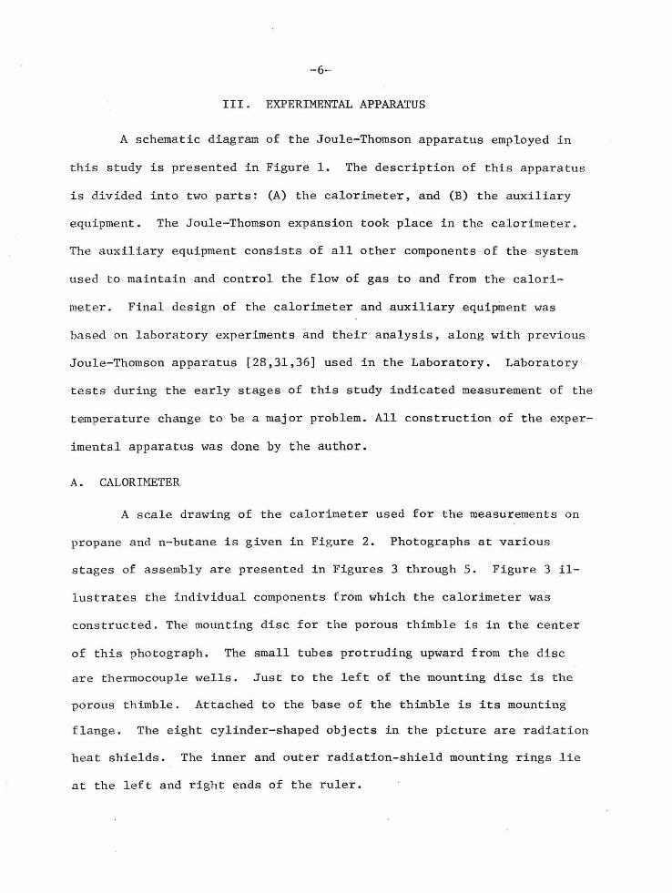
III. EXPERIMENTAL APPARATUS

A schematic diagram of the Joule-Thomson apparatus employed in

this study is presented in Figure 1. The description of this apparatus

is divided into two parts: (A) the calorimeter, and (B) the auxiliary

equipment. The Joule-Thomson expansion took place in the calorimeter.

The auxiliary equipment consists of all other components of the system

used to maintain and control the flow of gas to and from the calori­

meter. Final design of the calorimeter and auxiliary equipinent was

based on laboratory experiments and their analysis, along with previous

Joule-Thomson apparatus (28,31,36) used in the Laboratory. Laboratory

tests during the early stages of this study indicated measurement of the

temperature change to be a major problem. All construction of the exper­

imental apparatus was done by the author.

A. CALORIMETER

A scale drawing of the calorimeter used for the measurements on

propane a nd n-butane is given in Figure 2. Photographs at various

stage s of assembly are presented in Figures 3 through 5. Figure 3 il­

lustrates the individual components from which the calorimeter was

constructed. The mounting disc for the porous thimble is in the center

of this photograph. The small tubes protruding upward from the disc

are thermocouple wells. Just to the left of the mounting disc is the

porous thimble. Attached to the base of the thimble is its mounting

flange. The eight cylinder-shaped objects in the picture are radiation

heat shields. The inner and outer radiation-shield mounting rings lie

at the left and right ends of the ruler.

-7-

All parts of the calorimeter were easily assembled and

disassembled. Stainless-steel screws were used to hold the thimble and

mounting rings in place . The ease of assembly and disassembly permitted

the measurement of Joule-Thomson coefficients with different arrange­

ments of the radiation shields. Nitrogen and carbon dioxide were used

as test gases. These gases could be exhausted to the atmosphere . At

room temperature and atmospheric pressure, the values of their Joule­

Thomson coefficients were sufficiently different that they spanned the

anticipated range of the hydrocarbon measurements.

The mounting disc for the porous thimble was machined from a

linen-base, phenolic plastic. This plastic has excellent high­

temperature and chemical-resistance properties. It is easy to machine

and is also a good thermal insulator. The diameter and thickness of

the disc were limited by the size of the cavity in the pressure vessel

designed for measurements from 50 to 5000 psia. Since all unwanted

heat transfer occurred through this disc, it was made as thick as prac­

ticable. A Teflon mounting disc was also tested but the difficulty in

attaching thermocouple wells and exhaust tubing eliminated it from

consideration. After the gas passed through the thimble, it exited

from the calorimeter through the 0.814-inch hole in the center of the

mounting disc .

. Twelve 0.020-inch stainless-steel tubes protrude from the mount­

ing disc. They served as thermocouple wells for two separate thermo­

couple ne tworks. Three tubes with an angular spacing of 120° were

mounted at each of the four radial distances indicated for thermocouples

in Fi gure 2. With the calorimeter assembled, each thermocouple network

-8-

had three tubes inside the thimble and three outside. The ext ermtl

t lwrmocouple network consisted o.f three tubes at both the largest and

s mallest radial distance. The i.nternal network was compose d of the

remaining tuhes. 0 The external network was displaced by 60 angular

rotation to the internal network.

Thermocouples were easily removed from the thermocouple wells

without damage. The networks were also interchangable. This feature

eliminated early doubts as to whether different thermocouple readings

were due to differences in the networks or to temperature gradients

inside the thimble . The different lengths of the thermocouple wells

were due, in part, to the different heights of the radiation shields

which enclosed them. Measurement of the temperature change was made as

far away from the thimble mounting disc as practical. This reduced the

effects of any thermal gradients in the mounting disc. The thermo-

couple tubes were small in diameter to insure rapid response. In early

prot~types the thermocouple wells were open and the thermocouples were

epoxied in place . An erratic temperature in an early test was blamed

on gas leaking past the epoxy and jetting on the thermocouple junction.

Closed thermocouple wells prevented this problem with only a minor loss

in response time. The use of three thermocouples in series for each

thermoc ouple network was based on prior experiences in the Laboratory

and no other combination was tested.

Both thermocouple networks had copper-constantan junctions. All

thermocouple wire was 0.005-inch diameter and Teflon coated. Selection

of copper-constantan junctions was based on the greatest response to

temperature changes. Both thermocouple networks measured the

-9-

temperature of the gas after passing through the thimble relative to

the gas temperature before expansion. Therefore the measured t empera­

ture change was almost independent of the inlet or exit gas temperature

measurements.

The porous thimble used in this project was obtained from Coors '

Porcelain Company in Golden, Colorado. It was made from a fine-grained

alundum material. This thimble was machined on both its inside and

outside surfaces after receipt from Coors. Permeability tests on the

uncut thimble indicated that a wall thickness of 0.040 inch would

give a flow rate of 125 standard cubic feet of nitrogen per hour with a

pressure change from two to one atmospheres absolute. Machining of the

wall surfaces also improved the uniformity of the porous thimble,

thereby reducing the mixing problem. A small rim was left at the base

of the thimble for the flange mounting ring. The end of the thimble

was machined flat and then polished for a better seal at the thimble

mounting disc. A groove in the mounting disc centered the thimble and

confined the Teflon gasket used for the mounting seal.

Four thimbles, three alundum and one gold-platinum, were tested

in one or more of the four test calorimeters during the design stage.

All of the thimbles remained from the Joule-Thomson study on steam [36].

The shape of the porous surf ace was not tested as all of the thimbles

had the same basic shape. One attempt to test a spherical porous sur­

face ended in failure due to mechanical problems. A spherical porous

surface with a high ratio of porous surface to mounting surface is

theoretically a better design.

-10-

Tests with the alundum thimbles consisted of changing the w<ill

thickness and reducing the flow area by using an impervious coating.

The gold-platinum thimble was tested in three different conditions: as

received with its eighteen 0.006-inch diameter holes partially clogged ,

all eighteen holes opened, and all eighteen holes increased to 0.008-1

inch diameter. Test results with the gold-platinum thimble were

similar to the alundum thimbles except for larger fluctuations in the

measured temperature change. The larger fluctuations were contributed

to the mixing of the expanded gas. Two thermocouple networks, similar

to those previously described, measured the results of all tests.

At low flow rates both thermocouple networks indicated tempera-

ture changes smaller than anticipated. Agreement of nitrogen and carbon

dioxide with published values [9] improved with increasing flow rates .

An explanation of this result is explained later (see Thermodynamics

Analysis). In addition, the two thermocouple networks did not give

identical results when the calculated Reynolds number in the annular

region between radiation shields was in the laminar region (below

2000). The Reynolds number at a particular weight rate of flow of the

gas was change d by increasing or decreasing the number of radi ation

shields. At low Reynolds numbers , the interior thermocouple network

indicated a smaller temperature change than the external network . I f

this difference had been caused by thermal transfer, the external net-

work would have indicated the smaller change. The difference in values

was credited to poor mixing of the expanded gas. At flow rates with ·

Reynolds numbers above 2500, the difference was negligible and the gas

was assumed to be mixed.

/

-11-

The eight radiation-heat shie lds used in the calorimeter were

made of 0 . 001-inch brass shim stock. Five of the shields were nested

concentrically around the thimble . The other three were located con­

centrically within the thimble. The cylindrical shape of each

radiation shield was maintained by a small brass ring at one end of

the shield and the plastic mounting ring at the other end. The brass

ring had cross-sectional dimensions of 0.050 by 0.050-inch. All seams

were s olde red. A two-mil gold plating, both inside and out, was used

to prevent corrosion in future anticipated measurements. Primary

purpose of the radiation shields was to increase the turbulence of the

gas and to direct the flow past the thermocouples. The final design

and arrangement of the radiation shields were determined by several

factors . Le ngth of the radiation shields was limited by the dimen­

sions of the thimble and by the cavity of the high-pressure vessel .

The numbe r of s hields used was a compromise. Increasing the number of

shields between the thimble and the rmocouples reduced the fluctuations

i n thermocouple r eadings. De creasing the number of shields reduced

t he kinetic en erg y change. Two shields between the thimble and ther­

mocouples on each side of the thimble was the best arrangement tested .

Each radiation s hie ld was individually removable and electri­

cally insulated from the othe r shields. Removable shields made

possible a l arger number of tests. Electrically insulated shields

reduce d the possibility of the rmocouple shorts. The shields were

attached to the mounting rings by a press-fit and the n pinned to pre­

vent a ny slippage that might occur at the h igh e r temperatures of t he

tnvc s li.gat l.on. The gas f lowe d between shields in a n uxial direct.ion

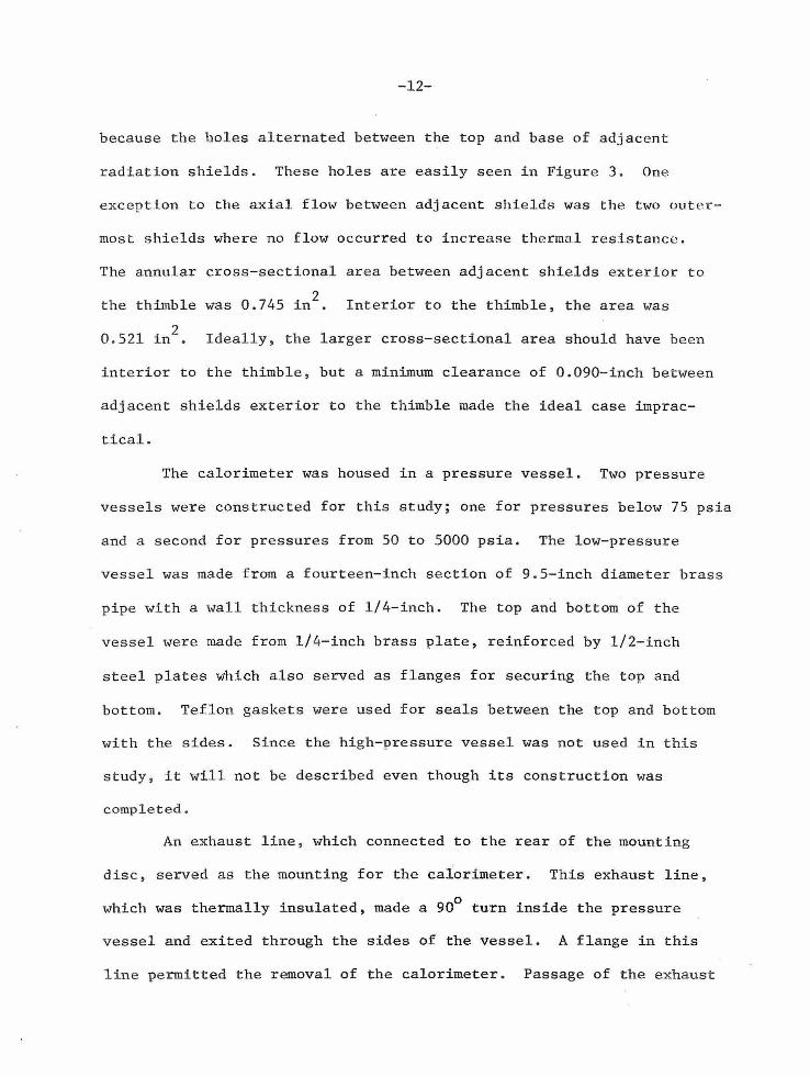
-12-

because the boles alternated between the top and base of adjacent

radiation shields. These holes are easily seen in Figure 3. One

except.ion to the axial flow between adjacent shields was the two outer-

most shields where no flow occurred to increase thermal resi.stance.

The annular cross-sectional area between adjacent shields exterior to

the thimble was 0.745 in2

• Interior to the thimble, the area was

2 0 .521 in • Ideally, the larger cross-sectional area should have been

interior to the thimble, but a minimum clearance of 0.090-inch between

adjacent shields exterior to the thimble made the ideal case imprac-

tical.

The calorimeter was housed in a pressure vessel. Two pressure

vessels were constructed for this study; one for pressures below 75 psia

and a second for pressures from 50 to 5000 psia. The low-pressure

vessel was made from a fourteen-inch section of 9.5-inch diameter brass

pipe with a wall thickness of 1/4-inch. The top and bottom of the

vessel were made from 1/4-inch brass plate, reinforced by 1/2-inch

steel plates which also served as flanges for securing the top and

bottom. Teflon gaskets were used for seals between the top and bottom

with the sides . Since the high-pressure vessel was not used in this

study, it will not be described even though its construction was

completed.

An exhaust line , which connected to the rear of the mounting

disc, served as the mounting for the calorimeter. This exhaust line,

which was thermally insulated, made a 90° turn inside the pressure

vessel and exited through the sides of the vessel. A flange in this

line permitted the removal of the calorimeter . Passage of the exhaust

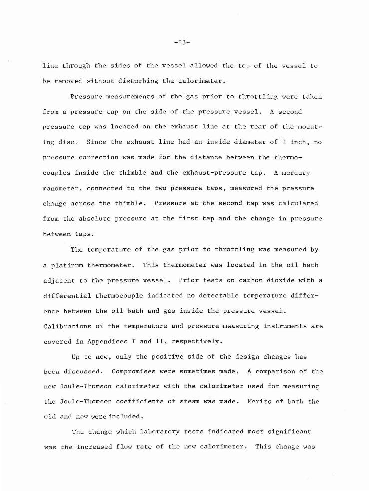
-13-

line through the sides of the vessel allowed the top of the vessel to

be removed without disturbing the calorimeter.

Pressure measurements of the gas prior to throttling were taken

from a pressure tap on the side of the pressure vessel . A second

pressure tap was located on the exhaust line at the rear of the mount~

i ng disc. Since the exhaust line had an inside diameter of 1 inch, no

pressure correction was made for the distance between the thermo­

couples inside the thimble and the exhaust-pressure tap. A mercury

manometer, connected to the two pressure taps, measured the pressure

change across the thimble . Pressure at the second tap was calculated

from the absolute pressure at the first tap and the change in pressure

between taps .

The temperature of the gas prior to throttling was measured by

a platinum thermometer. This thermometer was located in the oil bath

adjacent to the pressure vessel. Prior tests on carbon dioxide with a

differential thermocouple indicated no detectable temperature differ­

ence between the oil bath and gas inside the pressure vessel.

Calibrations of the temperature and pressure-measuring instruments are

covered in Appendices I and II, respectively.

Up to now, only the positive side of the design changes has

been discussed . Compromises were sometimes made. A comparison of the

new Joule-Thomson calorimeter with the calorimeter used for measuring

the Joule-Thomson coefficients of steam was made. Merits of both the

old and new were included.

The change which laboratory tests indicated most significant

wa s t h e increased f l ow rate of the new calorimeter . This change was

-14-

i ncorporated by reducing the wall thickness of the porous thimble from

0 . 125-inch to 0 .040-inch and by operating the equipment at p r essure

changes up to 8.6 psi. The increased flow rate through the calorimeter

made other changes necessary. These changes were primarily the result

of the increased volumetric flow rate, especially at low pressures .

The increased flow rate decreased the thermal-transfer correction ( see

Thermodynamics Analysis), response time, and mixing problems. On the

other hand, problems with kinetic energy changes, equipment size and

auxiliary-flow equipment resulted from the increased flow rate. To

reduce the kinetic energy change, a pressure vessel with large passages

and restricted for use at low pressures was necessary. This caused the

construction of a second pressure vessel with smaller passages to

reduce structural stresses at high pressure s. The changing of equip­

me nt in the middle of an investigation is not desirable .

Another change was the use of 0 . 001-inch brass radiation shields

in place of the 0.010-inch brass or 0.020-inch gold shields of the

steam calorimeter. The increased flow rates of the gas and smaller

mass of the radiation shields reduced the time to attain steady state

from days to hours. The smaller mass did not dampen temperature fluc­

tuations as well and this placed more stringent requirements on

pressure regulation. The use of equal annular areas between adjacent

radiation shields rather than equal radial distances improved the

accuracy of the kinetic energy calculations but complicated construc­

tion. The use of plastic instead of stainless-steel for the mounting

disc reduced thermal transfer and also the maximum operating temperature

of the calorimeter .

-15-

R. AUXILIARY EQUIPMENT

The components of the Joule-Thomson apparatus making up the

auxiliary equipment are shown in Figure 1. The auxiliary equipment

is described in the same order that the experimental fluid followed

as it flowed through the different components. The hydrocarbon gas was

stored as a liquid in one of the two high-pressure storage cyl-ln<lcrs.

Each cylinder held about 20 pounds of liquid hydrocarbon. The equip­

ment was arranged so that either cylinder could be removed or replaced

during an experiment without affecting the measurements. Each

cylinder was wrapped with an 800- watt tape heater. These heaters were

used to increase the vapor pressure of the liquid hydrocarbon . Vapor

pressure was the source of pressure for all experimental measurements.

Pressure gauges on each storage cylinder recorded the vapor pressure.

The output of the heaters was controlled manually by Variacs.

A l/4-inch copper tuhe connected the hydrocarbon cylinder

manifold to a vaporizer. The vaporizer consisted of about thirty f eet

of 1/4-inch copper tubing coiled around a twelve-inch length of 2-inch

o.d. brass pipe . Inside the pipe were about fifty feet of nichrome

heating wire coiled on a ceramic tube~ The vaporizer was installed

with the pipe i n a vertical position. A 1/4-inch copper tube connected

the vaporizer to a pressure regulator which was located about eighteen

inches above it. Additional 1/4-inch tubing connected the regulator

to a valve panel. This panel consisted of five valves and two

rotameters . The arrangement of this panel can be seen in Figure 1.

The rotameters were to determine the composition of gas mixtures.

-16-

The next component in the flow path was a Cartesian manostat

which regulated the pressure to the nearest 0.1 mm Hg. After passing

the manostat, the. gas entered a second electrical heater si.milar to

the va porizer and designated as a preconditioning he ate r. The gas

the n flowed through fifty feet of 1/4-i.nch copper tubing wl1ich was

submerr.~ed in the oil bath. After passing through the conditioning

tubing, the gas flowed into the pressure vessel which was also located

in the oil bath . The gas then flowed through the calorimeter and

passed from the pressure vessel through the exhaust line.

The oil bath and thyratron temperature modulator were of the

standard design used in the Laboratory.

After passing from the pressure vessel by a 1-1/4-inch o . d.

heavy-wall brass pipe , the gas flowed through a large throttle valve .

After the throttle valve, it flowed into one of two high-pressure

cylinders which were submerged in a dry ice - trichloroethylene mix­

ture. It was possible to remove and replace the receiving cylinders

during a measurement without disturbing the steady state. A vacuum

pump could be connected to the receiving cylinder manifold .

-17-

IV. EXPERIMENTAL PROCEDURE

The equipment used for the Joule-Thomson measurements has been

previously described (see Experimental Apparatus) . Measurements bega n

by setting the controls on the constant-temperature oil bath, which

contained t he Joule-Thomson calorimeter, for the desired temperature .

Usually four to eight hours elapsed until the i nterior of the calori­

meter came to thermal equilibrium with the oil bath . This elapsed time

could be reduced by a small flow of gas through the calorimeter. A

zero temperature change across the porous thimble was used as an i ndi­

cation of equilibrium. The liquid hydrocarbon was warmed by the

heaters on the high-pressure storage cylinders as the bath and calori­

meter were brought to temperature. Due to various line, valve , and

regulator pressure losses, the vapor pressure for any measurement was

norma lly 25 to 50 psi higher than the pressure at the inlet of the

calorimeter.

The hydrocarbon cylinde rs were inverted so that liquid rather

than vapor left the cylinder . This was necessary because the h eat of

vaporization at the liquid-gas interface was large . In tests with

carbon dioxide where the liquid-gas interface was inside the cylinder ,

large quantities of heat were required to maintain a constant cylinder

temperature . Temperature regulation was very difficult due to the

delay in response to changes in heater settings . Maintaining a con­

s t ant t emperature and vapor pressure inside the heavy-walled cylinder

improved pressure regulation.

-18-

When li.quid was removed from the cylinder, the li.qu l.d·-g11s

interface was outside the storage cylinder. The vaporizer with i ts

more efficient heat exchanger and faster response vaporized the liquid

and superheated the vapor. This latter feature was particularly

desirable. It prevented condensation of the gas cooled by the Joule­

Thomson expansion upon passing through the pressure regulator . During

start-up the superheat helped to heat the copper tubing between the

vaporizer and pressure r~gulator. The vertical position of the

vaporizer allowed any condensation to drain back to the liquid-gas

interface. The poor thermal conductivity of gases relative to liquids

aided temperature regulation at the vaporizer.

After passing from the vaporizer, the superheated gas entered

the pressure regulator used to maintain a pressure of about 10 psi

higher than that desired for the particular measurement . This extra

10 psi was removed by throttling the gas at the valve panel.

Throttling was necessary for the proper operation of the Cartesian

manostat located after the valve panel in the direction of flow. The

manostat controlled the pressure to 0.1 rmn Hg by bleeding off the

excess . The throttle valve reduced the volume of gas l ost at the

manostat . The amount was determined by bubbling through a beaker of

water. The optimum volume was the lowest that constantly bubbled

through the water . It amounted to a few cubic centimeters of gas per

hour .

After passing the manostat, the gas entered the preconditioning

heater which adjusted the gas temperature to that of the oil bath. A

-19-

mercury thermometer was used to de termine the init:i.al lieat..:~r s e t:t I ngH .

Final adjustments were determined by the automatic feature of the

thyratron temperature controller on the oil bath. If the gas tempera­

ture was too low after leaving the preconditioning heater and upon

entering the conditioning coil submerged in the oil bath, the bath

required more power to maintain a constant temperature than it did just

p r ior to the start of the gas flow. When the gas departed the precon­

ditioning heater at the proper temperature, the automatic controller

r eturned to its original setting. The conditioning coil in the oil

bath made the final temperature adjustment to the gas before entering

the calorimeter pressure vessel also submerge~ in the oil bath.

After entering the pressure vessel, the gas flowed into the

calorimeter and through the porous thimble. The pressure change and

the temperature change of the throttling process were measured in the

calorimeter . The exhaust pressure of the calorimeter was regulate d by

a large throttle val ve located approximately six feet downstream from

the calorimeter . When the throttle valve was completed closed ther e

was no pressure change across the thimble. By slowly opening this

valve, the desired pressur e change across the thimble could be obtaine d .

Remember that the upstream pressur e was controlled by the regulato r­

manostat and essent i ally independent of the downstream pressure . During

start-up this valve was always closed to prevent an excessive pressur e

c hange across the por ous thimbl e.

After passing through the large throttle valve , the gas entered

one of two high-pressure receivi ng cylinders. These cylinders wer e

evacuated prior to each experiment and submerged in a dry ice -

- 20-

trichloroethylene bath. The hydrocarbon gas recondensed and the vapor

pressure reduced to a few centimeters of mercury. This low pressure

extended hack to the large throttle valve in the exhaust line from the

calorimeter. The large pressure drop across this valve caused a sonic

velocity through it which eliminated the effects of any pressure fluc­

tuations in the receiving cylinders. Proof of this sonic velocity was

determined by adjusting valves on the receiving cylinder manifold

without disturbing the Joule-Thomson measurement. The condensation

process also acted as a leak detector for the measurements below atmos­

pheric pressure. Had any non-condensables leaked into the apparatus , it

would have would have i ncreased the pressure inside the receiving

cylinders .

Since both the storage and receiving cylinders could be replaced

during an experiment, the initial amount of liquid in the storage

cylinders was not a limiting factor. No run used more than 40 pounds of

hydrocarbon .

-21-

V. THERMODYNAMIC ANALYSIS

The Joule- Thomson coefficient of a fluid is defined as its

differential change in temperature with pressure at constant enthalpy

and composition. All apparatus for measuring Joule-Thomson coeffi­

cients as functions of temperature and pressure are basically similar.

A fluid maintained at a constant temperature and pressure is throttle d

unde r steady-flow conditions into a region of lower pressure. Only

measurements of temperature and pressure are required with the ideal

conditions of constant enthalpy and composition. However, a Joule­

Thomson expansion at constant enthalpy is most difficult due to thermal

transfer and kinetic energy changes within the experimental system .

Mathematical relationships to analyze the effects of non-constant

enthalpy on the Joule-Thomson coefficients are derived from thermodyn­

amics. Unlike the ideal case, the equations emphasize the effects of

the flow rate through the porous thimble on experimental measurements.

The model represents the limiting case for thermal transfer and was

used to evaluate the design and ope ration of the Joule-Thomson

apparatus . It was also used to analyze two methods of measuring Joule ­

Thomson coefficients and to correct previous Joule-Thomson measurement

for thermal transfer (see Resul ts).

To develop the mathematical relationships, an extension of the

Gibbs pha se r ule [27] was used as the starting point. The state of a

homogene ous f l uid of constant composition is a unique function of two

intens i ve variables. The temperature was considered a function of

pre ssure and enthalpy:

-22-

T f(P,H)

The total derivative of the temperature with .respect to pressure is

(dT/dP) tl pa i (()T/aP)H + ( ()T/()H)p (dH/dP) l . · pati (l)

The "path" is the course which the fluid takes as it flows between the

temperature and pressure-measuring devices in the throttling calori-

meter. Notice that the measured change in temperature with pressure is

path dependent, even though the Joule-Thomson coefficient, (()T/oP)H ,

is independent of the path. For small changes in pressure, Equation

(1) can be expressed as

(l:iT/l:iP)path (oT/oP)H + (l/C ) (l:iH/l:iP) h p pat (2)

where Cp is defined as (3H/3T)p .

The law of conservation of energy for a steady flow process was

used to evaluate l:iH . This law can be expressed

Q' - W' s

l:iH + l:i(P.E.) + l:i(K.E.)

where Q' and W' represent the thermal transfer and shaft work per s

pound of fluid. If the potential energy change is small and no shaft

work is performed, the above equation reduces to

Q' L\H + L\(K.E.) (3)

Solving for l:iH in Equation (3) and substituting the results into

Equation (2)

(6T/6P)path (3T/3P)H + (l/C ) {[QI - Ll(K.E.)] I L\P} h • p pat (4)

-23-

To calculate a value for the thermal transfer, Q' , it is neces­

sary to understand the mechanics of the throttling process . Thermal

transfer results from the temperature change of the expansion. Heat

is either added to or lost from the throttled fluid, according to

whether the fluid is cooled or heated upon expansion. Since the

expanded fluid is in contact with both the interior surf ace of the

porous thimble and the surface of the mounting disc enclosed by the

porous thimble, heat can be transferred through either surface. For

simplicity in calculation, thermal transfer through the walls of the

thimble and through the mounting disc were handled separately by

alternately assuming the other to be a perfect thermal insulator.

In the first case, the mounting disc for the porous thimble was

assumed a perfect thermal insulator, while the fluid and porous thimble

were treated as thermal conductors. The fluid, prior to passing

through the porous thimble, had a temperature and pressure of T1

and

P1

. The temperature and pressure of the fluid after passing through

the thimble were T2

and P2

• The fluid was assumed to have a

positive Joule-Thomson coefficient. Therefore T2

and P2

are lower

in value than T1

and P1

• Since the walls of the thimble and fluid

have finite thermal conductivities, a heat flux in the direction of

the fluid flow occurred across the thimble due to the temperature

change . No heat was lost by conduction through the mounting disc

since it was assumed a perfect thermal insulator. Therefore the source

of the heat transmitted by thermal conduction through the walls of the

thimble was from the fluid prior to passing through the thimble. The

-24-

fluid which released this heat was then cooler than T1 prior to being

throttled. However, all heat conducted through the walls of the

thimble must be returned to the expanded gas since no heat accumulated

in the walls and no heat was conducted through the mounting disc. The

expansion is isenthalpic and therefore the state of the throttled fluid

was uniquely determined by P2

and H2

• The net result was no change

to the Joule-Thomson measurements because of thermal transfer throug h

the walls of the thimble. Therefore a gold thimble would give the same

results as one of low thermal conductivity. A temperature gradient in

the fluid adjacent to the thimble was possible. Turbulence of the

fluid, aided by the radiation shields, reduced the effects of this

gradient on the experimental measurements to a non-detectable amount .

Thermal transfer through the mounting disc for the porous thimble

occurred because the expanded gas inside the thimble was cooler than

the inlet gas which was in contact with the external surfaces of the

mounting disc . If the temperatures of all surface areas of the thimble

mounting disc were known, it would be theoretically possible to calcu­

late the. thermal transfer through that part of the mounting disc

surface enclosed by the porous thimble. The amount of thermal transfer

would be calculated in BTU's per hour since no quantity used in the

calculation is relate d to the flow rate. The temperature change which

caused the thermal transfer is primarily a function of the pressure

change and Joule-Thomson coefficient of the fluid and almost indepe~dent

of the permeability of the porous thimble. Since "Q"' in Equation (4)

was given in BTU's per pound of fluid, it is related to the thermal

transfer calculated from the surface temperatures of the mounting disc

-25-

in BTU's per hour through the flow rate. This relation can be expressed

mathematically as

Q' QI;. (5)

. whe re Q is the thermal transfer in BTU's per hour and m the flow

rate in pounds per hour.

Substituting Equation (5) into Equation (4), the following rela-

tion was found:

(6T/6P) h = (ClT/ClP)H + (l/C ) {[(Q/;.) - 6(K.E.)] I 6P} pat p (6)

It is evident at this point that experimental measurements of the

Joule-Thomson coefficient are dependent on the flow rate due to non-

isenthalpic conditions. Rearranging Equation (6), one obtains:

(/1T//1P) h = caT/aP)H + Q/~c t:iP - !1(K.E.) / c 6P pat p p (7)

To aid in subsequent analysis, the last two terms on the right-

hand-side of Equation (7) will be designated by

c . Q

Q/{nc /1P p

c = 6 ( K . E.) I c /J.P /J.(K.E.) p

(8)

(9)

In the a bove equations, /J.P represents P2

- P1

and is negative.

Therefore the thermal-energy correction subtracts from the true value

of the Joule-Thomson coefficient and the kinetic energy correction

adds to the true value.

Before using Equation (7) to calculate numerical values of the

thermal a nd kinetic energy corrections for the apparatus used in this

-26-

study, the equation will be used to analyze two methods of mnasuring

Joule-Thomson coefficients.

One successful method of measuring Joule-Thomson coef fi c ·t c11 ts

has heen through the use of large pressure chang1.~s. These changL's

usually range from 300 to 1000 psi. Using large changes reduces the

percent error caused by instrumentation inaccuracies. It does not

reduce the thermal-transfer correction because the pressure change

appears in the denominator. As ~P is increased, ~T increases some­

what proportionally. The amount of thermal transfer increases with the

increase in ~T • However, the flow rate through the thimble also

increases and it is not off set by any term in t he numerator of Equation

(8) . The increased flow rate reduces the error in Joule-Thomson

coefficients measured with large pressure changes since the thermal­

energy correction is normally neglected due to the difficulty in

calculating values for the thermal transfer. Unfortunately the

resulting Joule-Thomson coefficients are integral values, and the dif­

ferential coefficients must be calculated. The calculations introduce

errors to the differential coefficient, thereby reducing a part of the

advantage of the method. A major disadvantage is that measurements

nea r zero pressure are not possible.

A second successful method of measuring Joule-Thomson coeffici­

ents has been to use small pressure changes of less than one atmosphere .

It is assume d that the differential Joule-Thomson coefficient is

uwasure d direc tly by this method. Small pressure changes are usually

accompanied by small volumetric-flow rates . Small volumetric-flow

rates result in even smaller weight-flow rates at low pressures. As

-27-

the weight-flow rate approaches zero, the correction due to thermal­

energy transfer approaches infinity if the pressure change remains

constant. This result can be detennined from Equation (8). Therefore

the method of small pressure changes is subject to large. errors at low

pressures.

This particular study used the method of small pressure changes

but incorporated one feature of the large pressure change method. The

por ous thimble had very thin walls so large flow rates could be

obtained at low pressures. Flow rates up to five pounds per hour were

obtainable below atmospheric pressure. Several problems occurred as a

result of the high flow rates. Large passages in the calorimeter were

required to reduce kinetic energy changes. These large passages made

necessary the construction of a second pressure vessel with small

passages for high pressures. Pumping large volumes of low density

gases caused many problems. This was solved by a single-pass evapora­

tion-condensation pumping system . Other than mechanical problems,

the method of small pressure changes combined with large flow rates

has no major disadvantages. Its most important feature was its high

accuracy in the low pressure region where the other methods are not

possible or are subject to large inaccuracies.

As the correction factors for thermal transfer and kinetic

ener gy changes are path dependent, the following numerical calculations

apply only to the equipment used in this study. The principle is

applicable to most Joule-Thomson apparatus. The first correction to be

inspected will be that due to kinetic energy changes.

-28-

Kinetic energy changes were caused pr:f.marLly by changfls :l.n thC'

specific volume of the gas resul ting from the pressure change . SJncc

the slope of the specific volume versus pressure curve of a gas

increases with decreasing pressure, the largest changes in volume

occurred at the lowest pressure for a particular !J.P • This result

can be seen from the ideal gas law:

d(V)/dP d(RT/P)/dP

Some of the larger pressure changes in this study occurred at the

lower pressures to increase the weight-flow rate through the thjmble .

Three assumptions were used in the correction for the kinetic

energy change: the ideal gas law is applicable, average velocities can

be used , and the temperature change due to the throttling can be

neglected . At low pressures and small temperature changes, all three

assumptions are reasonable . The gas flowed in the annular space

between the radiation shields before and after the Joule-Thomson

expansion. The cross-sectional area between adjacent shields exterior

to the thimble was 0.745 in2

• Interior to the thimble it was 0.521 in2 .

Changes in kinetic energy per pound of fluid can be expressed

in terms of average velocities by

!J. (K.E.)

·where and are the velocities of the gas before and after

throttling, and gc is the gravitational constant. Substituting

Equation (10) into Equation (9), one obtains

(10)

2 C = (u2 Li(K.E.)

-29-

2 u

1) I 2g C LiP

c p

Incorporating geometrical factors of the calorimeter and using the ideal

gas law, it results that

The maximum kinetic energy corre ction occurred in a propane experiment

where P1

= 12.30 psia, P2

= 3. 72 psia, T = 740°R and

C 0 . 522 BTU/lb 0 R . U i th 1 th 1 ti t E t ' s ng e se va ues , e so u on o •qua 1on

n

( 11) is

. 2 -5 0 Cli(K.E.) = - 5.89 m x 10 R/psi

Since the flow rates at the above conditions was 3.31 pounds per hour ,

the kinetic energy change correction was 6.4 x 10-4 0

R/psi or about

0.8% of the measured coefficient. (Propane at 280°F and 8.01 psia

has a Joule-Thomson coefficient of 0.07986°F/psi). At 15.38 psia and

280°F, the kinetic energy correction decreased to approximately 0 . 38%

of the measured coefficient even though the flow rate was increase d

to 7 pounds per hour .

. An exact calculation of the therma l transfer, Q , is virtually

impossible but an estimate of the upper limit was made. Four assump-

tions were necessary: (1) the throttled fluid was assumed to be in

thermal equilibrium with the surface of t he mounting disc enclosed by

the porous thimble, (2) all other surfaces of the mounting disc were

at the t emperature of the inlet gas, (3) the expanded gas was perfectly

mlxed and (4) the cylindrical mounting disc could b e approximated by a

-30-

bar of the same cross-sectional profile and equivalent heat-transfer

areas on the top and bottom . Using these assumptions, the temperature

profile of the mounting disc was determined nume rically using a relaxa-

tion me thod described by Dusinberre [38). A one-eighth inch square

grid was used in the calculations . A solution was determi ned for a

dimensionless temperature defined by

The resulting temperature profile for a radial cross-section of the

mounting disc is given in Figure 6. A value of (t:,0/t:,y) was found Yo

to be -0.888/inch where y is the coordinate direction perpendicular

to the lower surface of the mounting disc and y0

represents the lower

surface.

The thermal transfer into the interior of the thimble was calcu-

lated from the equation:

Q -kA (dT/dy) o yo

kA 6T (N/J/ t:,y) o Yo

(12)

where 6T Substituting Equation (12) into Equation (8)

CQ· = [kA (t:,0/t:,y) ](l/C )(l/~)(t:,T/t:,p) o yo P

(13)

The term in the brackets is constant for any particular apparatus

since it depends only on the materials of construction and shape of the

heat transfer surface . It was calculated for the case where

A 0

1. 885 in2

, -3 0 k = 8.5 x 10 BTU/hr-in- F, and

-0.888/inch. The result of this calculation was

..-Jl-

c· = ~-0.014(1/C )(l/~)(~T/~P) 0~/psi Q p

The percent of the Joule-Thomson coefficients given by the thermal-

energy correction is

(14)

Equation (14) implies that a gas with a C = 0.5 BTU/lb-°F and flow­p

ing through the thimble at a rate of 1 pound per hour would result in

a Joule-Thomson coefficient that is too small by 2.8%. Between 100

0 and 280 F, the constant pressure heat capacity of both propane and n-

butane at zero pressure range between 0.4125 and 0.5225 BTU/lb-°F ,

according to Rossini [39) .

Returning to the same example used in the kinetic energy correc-

tion (propane at 280°F and 8.01 psia with C = 0.522 BTU/lb-°F p

and

m = 3.31 pounds per hour), the thermal energy correction is

-4 0 -6.45 x 10 F/psi or -0.81% • At 15.38 psia, the thermal energy

correction reduces to -0.383% . Since the thermal energy correction is

approximately equal to the kinetic energy correction in the region

where the corrections are large, it was assumed that the correcti ons

cancelled each other and were not applied to the experimental data

points. The experimental apparatus was deliberately operated so that

the corrections would cancel each other in the low pressure region. The

flow rates ranged between 3.31 and 11 .5 pounds per hour.

-32-

VI. CALCULATIONS

The Joule-Thomson coefficients,(~T/~P)H, were computed by

approximating the differential changes in temperature and pressure

with small finite changes. These changes were limited to a maximum of

0 1.5 F and 8.6 psi and they were measured directly. Changes in tempera-

ture were measured by differential thermocouples and changes in

pressure were measured by a differential mercury manometer .

The temperature and pressure of each Joule-Thomson coefficient

was determined by the arithmetical mean of the inlet and exhaust values.

The temperature of the gas at the inlet of the calorimeter was measured

by a platinum-resistance thermometer. The inlet pressure was measured

by a mercury manometer when below three atmospheres absolute. The

laboratory pressure balance [40] was used to measure the inlet pressure

when above three atmospheres. The exhaust temperature and pressure of

the gas were computed from the inlet values minus the change in value

due to throttling. Calibration and corrections to the temperature-

measuring devices are covered in Appendix I. Pressure information is

given in Appendix II.

Corrections to the measured Joule-Thomson coefficients due to

thermal transfer and kinetic energy changes were calculated previously

(see Thermodynamic Analysis). These corrections were found to be less

than 0 . 8 percent and essentially equal in magnitude. Neither correction

was applied to the measurements since they tended to cancel each othe r .

Therefore all Joule·-Thomson coefficients were calculated by dividing

the measured temperature change by the measured pressure change .

-33-

Unfortunately the e ase of calculating a single Joule -Thomson

coeff i c ien t was complic a t ed by r e lating several coeffici.ents to t he

same isotherm. The temperatu r e of each coefficient was related t o t h e

measured temperature change . This change could only be estimated for

a particular pressure change prior to the measurement . It was not

fea sible to constantly adjust the temperature and pressure to obtain

the desi red values since the equipment was operated with a single pass

of the gas . Therefore the resulting temperature of the coeffici ent

never fell on a parti cular isotherm but only in the c l ose vicinity. A

sma ll temperature correction was necessary to place a data point on

the nearest isotherm . 0

This correction was usually less than 0 . 2 F.

I t was obtained graphically from a rough temperature versus Joule-

Thomson coeffic ient plot.

Since the l00°F isotherm for n-butane did not plot as a str aight

line , a correction was made for the difference between the e x per ime nt-

ally measured integral and the desired differential Joule- Thomson

c oeffic ient resul ting from the finite pressure change . The e x p e ri-

me ntal da ta points we r e fitted to an e quation of the form ,

µ = a ' + b'P + c ' P2

( 15)

where t he constants a ' , b ' and c' wer e dete rmine d by a least -square s

f it and p 2

f udP

p l '1T/'1P (16) µ -

f 2 dP

p l

-34-

Results of the curve-flt are given in Table 3 and numerical values

of a', h' and c' are gi.ven in Table 5.

It was assumed that the desired l00°:F i.sotherm of differentlal

coeffici.ents would fit an equation similar to Equation (15):

a + bP + cP 2 • (17)

Upon substituting µ of Equation (17) into Equation (16) and inte-

grating between the inlet pressure P1 and the exhaust pressure P2

,

the following relationship for µ was found

p2

f (a + bP + cP2

) dP

µ pl

dP

(18)

Since the pressure of µ was the arithmetical mean of P1

and

P2

, the differential Joule-Thomson coefficient was determined for

this mean pressure by Equation (17):

(19)

Using Equations (18) and (19) to determine the difference between µ

and µ ,

For a first approximation of c , the value of c' determined from the

-35-

integral data points was used. Differential coefficients were then

calculated for each integral coefficient in the l00°F isotherm by the

relationship

µ = µ (µ - µ)

The calculated differential coefficients were then fitted to Equation

(17) and a new value of c was determined. The new value of c was

-5 1.090614 x 10 and it compared favorably with the value of c' which

- 5 was 1.092818 x 10 ; therefore no further iterations were made. The

calculated values of µ and numerical values of a, b, and c are

given in Tables 3 and 5, respectively.

-36-

VII. ERROR ANALYSIS

Error in the values of the Joule-Thomson coefficients was

directly related to the accuracy of the temperature and pressure

measurements . Equipment limitations and non-isenthalpic conditions

were the primary cause of error in both the absolute value and relative

change in temperature and pressure values .

In Appendix I, error in the measurement of the Joule-Thomson

t emperature due to instrumentation inaccuracies was calculated to be

l ess than 0.052°F. A change of 0.052°F in the temperature of the

coefficient could result in a difference of 0.03 percent in the Joule­

Thomson value . Error in the thermocouple readings used in the calcu­

lation of the temperature change of the Joule-Thomson expansion was

found to be less than 0.30 microvolt. Since the smallest thermocouple

r eading was larger than 40 microvolts, the error in thermocouple

measurements would cause an error of less than 0.7 percent in the

Joule-Thomson values.

In Appendix II, errors in the absolute pressure and the pressure

char ge used in the calculation of the Joule-Thomson coefficients were

es timated to be less than 0.1 psi and 0 . 05 mm Hg, respectively. A

pressure error of 0 .1 psi would cause a maximum difference of 0.03 per­

cent in the Joule-Thomson coefficients. Since the smallest pressure

change was 125 mm Hg, an error of 0.05 nun Hg would result in a maximum

error of 0 . 04 percent in the Joule-Thomson values.

Fluctuations in the pressure and pressure change due to the

controlling manostat were less than 0.1 mm Hg. A pre ssure-change fluc­

tuation of 0 .1 mm Hg could result in an error of 0.08 percent of the

-37-

Joule-Thomson value. Since these fluctuations could cause a Joule

effect of the same magnitude to be superimposed on the Joule-Thomson

fluctuation, the 0 . 1 nun Hg pressure fluctuation might induce an error

of 0.16 percent of the Joule-Thomson coefficient.

The e rrors in the Joule-Thomson coefficient due to thermal

transfer and kinetic energy changes were previously calculated (see

Thermodynamic Analysj_s) to be less than 0.8 percent of the Joule­

Thomson values. They were approximately equal in value and tended to

cancel each other. An error of less than 0.4 percent was assumed by

cancelling the thermal transfer with the kinetic energy change.

Impurities in the propane and n-butane used in this study were

determined by chromatographic analysis and listed in Table 9. The

purity of the propane and n-butane was found to be 99.91 and 99.66 mol

percent, respectively. Closely related hydrocarbons composed the major

i mpurities . Rased on the results of the Joule-Thomson coefficient of

mixtures of methane-ethane and methane-n-butane by Sage [32,331 and

nitrogen-ethane by Stockett and Wenzel [41], an error of less than

0.1 percent of the Joule-Thomson value was attributed to impurities.

The weight rat e of flow through the porous thimble was determined

by weighing the storage cylinders before and after each experimental

measurement. The esti mated error in the weights was approximately five

percent. Since the thermal transfer and kinetic energy change which

used the weight flow rate were assumed to cancel each other, no addi­

tional error was attributed to error in the flow rate through the

thimble.

-38-

The maximum error in the Joule-Thomson coefficients was deter­

mined by adding the individual errors which were:

Source

Temperature

Temperature change

Pressure

Pressure change

Pressure fluctuations

Non-isenthalpic conditions

Impurities

Total

% Error

0.03

0.70

0.03

0.04

0.16

0.40

0.10

1.46

Therefore the maximum error was less than 1.5 percent of the measured

Joule-Thomson coefficient.

-39-

VIII. RESULTS

Joule-Thomson measurements were made on gaseous propane at tern-

0 peratures from 100 to 280 F and at pressures from 8 to 66 psfa.

Joule -Thomson measurements were also made on gaseous n-hutane at tem-

0 peratures from 100 to 280 F and at pressures from 8 to 42 psia.

Results of these measurements are given for propane in Table 1 and for

n-butane in Table 3 . Corrected values of the coefficients, determined

by a l east-squares fit of the experimental points, are included in

these tables. The results are also given in graphical fonn in Figures

7 through 10. For propane, Figure 7 indicates the relationship between

the Joule-Thomson coefficient and pressure at constant temperatures.

Figure 8 indicates the Joule-Thomson coefficient versus temperature at

constant pressures for propane . For n-butane, Figures 9 and 10 show

similar relationships. A temperature interval of 60°F was used

between isotherms. The pressure interval between experimental points

varied but usually ranged from 10 to 20 psi.

A differential Joule-Thomson coefficient was assumed to have

been measured directly, since small finite changes in temperature and

pressure were used. (Other types of Joule-Thomson coefficients are

"integral" and "isothermal" which is defined as (aH/ClP)T .) Tempera­

o ture changes of 1.0 F and pressure changes from 3 to 8 psi were

typical . The pressure listed for each coefficient was the aritlunetical

mean of the inlet and exhaust pressures of the calorimeter. For

example, a Joule-Thomson coefficient listed at 8 psia might have been

measured with an inlet pressure of 12 psia and an exhaust pressure of

-40-

4 psia . Each isothe rm of Joule-Thomson coefficients in Figures 7 ancl

9 is experi mentally valid from the lowe st exhaust pressure to the

highest inlet pressure. The limits of the experimental range are

indicated by the solid lines in the above f igures .

All of the measured Joule-Thoms on coefficie nts were positive

and increase d in value with increasing pressure and mole cular weight.

The coeffi cients decreased in value with increasing temperature . Each

liste d Joule-Thomson coefficient in Tables 1 and 3 is the result of

approx imately 10 i ndividual points taken during the approach to steady

state over a time period ranging from 4 to 10 hours. Most of the

points during the approach to steady state were taken at thirty-minute

intervals starting about two hours aft e r the start of the throttling

process. Figure 13 indicates the individual points from which one

point in Table 3 is composed. An experimental measurement was ter­

minat e d when the difference in the ratio of ~T to ~p for five

consecutive points was l e ss than 0.3 percent.

Previous calculations (see Error Analysis) indicated the meas­

urements to have a maximum error of less than 1 . 5 percent. No point ,

after bei ng corrected for temperature , deviated from its isotherm by

more than 1.04 percent. Figures 7 and 9 compare the results of this

study with previous measure me nts for propane [28 ) and n-huta n e [29],

respectively. For propane, the agreement was within 5 percent ove r

the duplicated range. The results for n-butane disagree d to a l a rger

but varying extent. The greatest difference occurred when extrapolat­

ing the data to z e ro pressure. Values of the zero pressure Joule­

Thomson coefficient for the present and pre vious studies for n-butane

-41-

on the l00°F isotherm were 0.2563°F/psi and 0.1952°F/psi, respect ively.

This is a difference of approximately 26 perce nt. A very definite

trend was detectable between the present and previous n-b11tane coeffi-

cients. Agreement improved with increasing temperature and pressure .

This trend is a possible clue as to the reason for the discrepancy.

In the earlier study, a constant-volume cam pump was used as

the pressure source for all measurements. This pump had a small weight

rate of flow near atmospheric pressure and no correction was made to

the data for thermal transfer. It was previously shown (see Thermo-

dynamic Analysis) that the error in experimental Joule-Thomson

coefficients resulting from thermal transfer can be expressed by

C· Q

Q/(~C liP) p

(8)

where K = kA (lir/J/ liy) . 1 o y

0

Application of this correction for thermal

transfer to the n-butane data of the previous study would improve the

agreement with the present study. However, the lack of flow rate data

from the previous study prevented the straightforward use of Equation

(8). An estimate of the heat transfer correction was obtained in the

following manner. It was observed in the laboratory logbook that all

the previous data were measured at a pressure change of approximately

1.0 psi . A pressure change of 1.0 psi would result in a certain

volumetric flow rate which is almost i ndependent of the fluid density .

This is evident from Darcy ' s law [42) which can be expressed

V' - £ A(liP/lix)

where V' is the volumetric flow rate, £ the permeability of the

-42-

porous material and LiP/Lix the pressure gradient. Therefore it was

assumed t l;at the volumetric flow rate was constant for all previous

n-butane measurements.

For an ideal gas, the relation between the mass and volumetric

flow rate is

m V'p V'P/RT (20)

where p is the gas density and R the gas constant. Subt:; tituting

Equation (20) into Equation (8), the following relationship was ob-

ta.ined:

C· Q

(21)

To further simplify Equation (21) , changes in gas properties due to

thermal effects were assumed to change in a constant ratio. Therefore

Equation (21) can be expressed by

To obtain a value for c1

it was further assumed the primary

reason for the differences between the Joule-Thomson coefficients for

n-butane of the two studies was thermal energy transfer. In particular

a value of c1

was chosen to cause perfect agreement between the

J oule-Thomson coefficients of the two studies at 160°F and 14.7 psia.

The value calculated for c1

was 1.79 psi . Using this value, a

correction was made to all n-butane values. Results of these

-43-

corrections are given in Table 12 and Figure 14. All of the corrected

0 Joule-Thomson values, except those of the 220 F isotherm, then agree d

with the present study. If the experimental values of the 220°F were

multiplied by 1.105 prior to the application of the correction, excel-

lent agreement with thi.s isotherm would have been obtained. This

additional correction of 1.105 could have been caused by an error in

the pressure change of exactly 0.100 psi or a bath temperature of

120.00°F instead of 220°F. Anything which would affect the 6T/6P by

1.105 is possible. No single correction which might result from

experimental error was found that would correct the 220°F isotherm

without using the thermal-transfer correction.

A similar correction was not applied to the previous propane

values because the original data points were observed at considerably

higher pressures. The two-phase region for n-butane at l00°F starts

at 51. 4 psia. Therefore all experimental points were taken between

14.8 and 50 psia. For propane, twelve of the fifteen original data

points were taken between 50 and 550 psia. Since the smoothed data

reflected the influence of the higher pressure s where the thermal-

transfer correction would be small, a correction was not attempted.

It was observed that if the previous propane data were extrapolated

from the high-pressure region towards zero pressure by a straight line,

better agreement between the two studies would be obtained.

Since no other experimentally measured values of the Joule-

Thomso n coefficient for propane or n-butane were found, values were

calculated from other p-v-t data. One value of the Joule-Thomson

-44-

coefficient for prooane at 50 psia and 200°F was calculated from an

experimental isothermal throttling coefficient and heat capacity give n

in a recent paper [43]. This value was compared to an equtval~nt

value from this study and also the previous propane study. The results

of this comparison were 0.1154, 0.1158 and O.ll65°F/psi, respectively .

Joule-Thomson coefficients were calculated from the Benedict­

Webb-Rubin equation [11] with its original coefficients. Derivation

of the equation used to calculate the coefficients is given by Ahlert

and Wenzel [44] and consisted of the straightforward but lengthy proce­

dure of substituting the B-W-R equation into Equation (2). Results of

the calculations for propane and n-butane are listed in Table 7. A

comparison of the calculated coefficients with the coefficients of

this study and also the previous study are given in Figures 7 and 9.

The calculated coefficients from the B-W-R equation were larger in

value than the equivalent coefficients of this study. All isotherms

of the Joule-Thomson coefficients for both propane and n-butane,

except the 220°F n-butane isotherm of the previous study, indicated

the same general trends. This 220°F isotherm was lower in value than

anticipated for all pressures.

Since the greatest difference in the Joule-Thomson coefficients

of the experimental studies occurred when extrapolated to zero pres­

sure, a comparison with other p-v-t data was made at attenuation.

McGlashan and Potter [45] experimentally measured the second virial

coefficients of six alkanes from propane to n-octane. They expressed

their results by the following empirical equation:

Il/V c

-45-

0.430 - 0 .886(T /T) - 0.694(T /T)2

-0.0375(n-l)(T /·o 4·

5 c c c

(20)

where B is the second virial coefficient, V the critical volume, c

T the critical temperature and n the number of carbon atoms. Second c

virial coefficients calculated from this equation were compared with

second virial coefficients calculated from experimental p-v-t data on

methane through n-octane of numerous authors. For propane and n-butane

the p-v-t data of seve n different studies were used [46,47,48,49,50 , 51,

52]. The results of this comparison were given in graphical form by

McGlashan and Potter [45] . Unfortunately no tabular results were given

but a visual inspection of the graphs indicated the empirical equation

to yield values of the second virial coefficients which favorably agreed

with those calculated from the p-v-t data. 0 In the 100 to 280 F range

second virial coefficients calculated from the p-v-t data were slightly

larger (smaller negative values) than those calculated from the

empirical equation. The deviation increased with molecular weight from

about one percent for propane to approximately ten percent for n-hexane.

For n-butane, second virial coeff i cients calculated from the empirical

equation were too small by approximately two percent .

At low pressures the second virial coefficient is related to the

Joule-Thomson coefficient by the following equation:

µ (21)

Substituting Equation (20) into Equation (21), Francis and Luckhurst

[12] obtained the following equation for calculating zero pressure

Joule-Thomson coefficients:

0 1-1

-46-

(V /C0 )(0.2063(n-l)(T /T) 4 •5 + 2.082(T /T) 2 + 1.772(T /T) - 0.430 c p c c c

where the superscript 110

11 refers to zero pressure. They compared

Joule-Thomson coefficients calculated from this equation to experimental

Joule-Thomson coefficients. The comparisons indicated the above equa-

tion yielded Joule-Thomson coefficients which agreed with other

experimentally measured Joule-Thomson coefficients, both hydrocarbon

and inorganic, except for the propane and n- butane coefficients of the

previous study. Zero pressure Joule-Thomson coefficients from this

study compared favorably with the above equation. The results of these

comparisons are given in Table 6 and Figures 11 and 12. The comparison

indicated a maximum difference of 1 . 5 percent for propane and 2.8

percent for n- butane. The differences are in the proper direction to

agree with the p-v-t data for propane and n-butane (46 through 52]

whichMcGlashan andPotter used to compare with their empirical equation.

The Joule-Thomson apparatus used in this study was built from

the experience gained from two previous Joule-Thomson studies [28,36]

and considerable laboratory testing . A detailed description of the

equipment has been given (see Experimental Apparatus). The most sig-

nificant difference between this and other Joule-Thomson apparatus was

the high weight rate of flow below atmospheric pressure. The high

flow rate reduced the error due to thermal transfer in the low pressure

region.

-47-

IX. CONCLUSIONS

The measured Joule-Thomson coefficients of this study did not

agree with previous experimental values for .n-butane, which were shown

to be in error . The disagreement increased with decreasing pressure

to a maximum of approximately twenty-six percent at zero pressure

absolute. When a thermal-transfer correction was applied to the pre­

vious values, a satisfactory agreement was obtained except for the

220° isotherm. This isotherm did not conform to the general trends of

the other isotherms when compared to the experimental values of this

study or calculated values from the Benedict-Webb-Rubin equation. The

main value of Joule-Thomson coefficients calculated from the B-W-R

equation was to point out inconsistencies in experimental values

rather than any claimed accuracy of the calculated coefficients.

If a correction were made to the ~T/~P ratio of the 220°F

isotherm of the previous study for the type of error that would be

caused by inaccuracies in the pressure change, bath temperature,

thermocouples , etc., and then the heat-transfer correction applied,

the isotherm could be made to agree with this study.

For propane, the agreement between the present and previous

studies was acceptable. The high concentration of data points above

50 psia could explain the better agreement. At pressures where the

fluid density is appreciable, the thermal transfer correction is

small.

Joule-Thomson coefficients calculated at zero pressure absolute

from the equation of Francis and Luckhurst [12] agreed within 2.8

-48-

pe rce nt for bot h propane and n-butane values of this study . The e qua-

tion was shown to represent the p-v-t data of various authors on

ethane through n-octane within a narrow error band. The excellent

a g reement at zero pressure is signific ant,for the low pressure r e gion

is the most difficult in which to measure Joule-Thomson coefficie nts .

All isothenns of the measured Joule-Thomson coefficie nts of

0 this study for both propane and n-butane, exce pt the 100 F n-butane

isotherm, are plotted as straight lines. Based on the previous Joule -

Thoms on me asurements and also the B-W-R equation, all isothenns might

have some curvature toward higher values at higher pressures. Except

f o r the l00°F isotherm for n-butane, no curvature was detected at the

pressures of this study.

Since the slopes of the isothenns of the previous Joule-Thomson

measurements are larger than those of this study, one might e xpect the

da ta to diverge at higher pressures . If the thennal-transfer corre c-

tion i s applied to the previous values, the slopes are approx imate ly

equal . There fore the data would not dive rge .

The improved values of the present study is not only due to

instrume ntation improvements s i nce 1935 but also to changes in calori-

me t er design . The mos t signifi cant improvement was the incre ase d flow

thr ough the por ous thimble at low pressures . The equations used t o

r e late errors in the values of e xperimentally measured Joule-Thomson

coeff i c i e nts to the flow rate through the thimble are unique in tha t

the J oul e-Thomson coeffic ient was previously though t to be e s sential ly

inde pend e nt o f e x t ensive mea surements [53] • •

-49-

X. FUTURE WORK

Two areas of continued study with the present equipment are

desirable. First, using the high-pressure vessel not used in this

study; an increased pressure range for propane and n-butane would

permit a comparison of measurements where all flow rates are high.

Second, an increase in the number of hydrocarbons measured would be

benef i.cial to correlations between macroscopic measurements and micro­

s copic properties. Experimental Joule-Thomson data on higher-molecular

weight-normal hydrocarbons, isomers, and mixtures are very sparse.

Present values for iso-butane [10,54) are significantly lower than the

values of n-butane. No experimental Joule-Thomson measurements for any

other hydrocarbon isomer were found .

The most beneficial change to the equipment would be to replace

the evaporation-condensation single-pass flow with a recirculating

pump. This change would permit the determination of several data points

per day rathe r than two per week. A large-capacity diaphragm pump s eems

most feasible . Several pumps in parallel might be required at low

pressures . A metallic diaphragm, or possibly one made of some new

miracle polymer material, would be necessary to prevent contamination

of the hydrocarbon at high temperatures .

-50-

XI . REFERENCES

1. J. H. Potter, "Some Recent Throttling Investigations," §~-~on!:!_ Symposium on Thermophysical Properties, Princeton, N.J., 1962, pp 83-87.

2. J. 0. Hirschfelder , R. B. Ewell and J. R. Roebuck, "Determination of Intermolecular Forces Joule-Thomson Coefficients," ~Chem . Phvs . 6, 1938, pp 177A and 205-218.

3 . M. Klein, "Determination of Intermolecular Potential Functions from Macroscopic Measurements," J. Research of NBS, A. Physics and Chemistry 70A, 1966 , pp 259-269.

4 . J. O. Hirschfelder and W. E. Roseveare, "Intermolecular Forces and the Properties of Gases," J. Phys. Chem. 43, 1939, pp 15-35.

5 . T. Ishikawa, "Application of the New Equation of State of the Joule-Thomson Effect," Bull. Chem. Soc. Japan 26, 1953, pp 529-531 .

6. J. O. Hirschfelder, C. F. Curtis and R. B. Bird, Molecular Theory of Gases and Liquids, John Wiley & Sons, 2nd Printing, 1965, pp 2-3 .

7 . J. O. Hirschfelder, C. F. Curtis and R. B. Bird, Molecular Theory of Gases and Liquids, John Wiley & Sons, 2nd Printing, 1965, pp 173-177.

8. F. F. Hung, "Determination of Virial Coefficients and Derivatives from Free Expansion Data--with Application to Nitrogen," Proc . 3rd Symp . on Thermophysical Properties, Papers., Lafayette, Ind., 1965' pp 98-103 .

9 . R.H . Perry, C.H. Chilton and S. D. Kirkpatric,Perry's Chemical Engineers' Handbook, 4th Ed . , McGraw-Hill, New York, 1963, p 3-98.

10 . F . S. Manning and L . N. Canjar, "Joule-Thomson and Second Virial Coefficients for Hydrocarbons," J . Chem. Eng . Data 6, 1961, pp 364-365.

11 . M. Benedict, G. B. Webb and L. C. Rubin, "An Empirical Equation for Thermodynamic Properties of Light Hydrocarbons and their Mixtures ; Constants for Twelve Hydrocarbons," Chem . Eng. Prog . 47, 1951, pp 419-422.

12. P. G. Francis and G. R. Luckhurst, "Joule-Thomson Coefficients and the Principle of Corresponding States," Trans. Faraday Soc . 59, 1963 , pp 667-672.

-51-

13. J. P. Joule and W. Thomson , "On the Thermal Effects of Fluids in Notion--Par t IV," _Phil. Tr. Roy. Soc . 152, Part 2, 1862, pp 579-589.

14. J. P . Joule and W. Thomson, "On the Thermal Effects Experienced by Air Rushing through Small Apertures," Phil. Mag. Ser . 4, 4, 1852, pp 481-492.

15. H. L. Johnston and D. White, "VII--A Summary of Experimental Deter­minations of Joule-Thomson Effects in Gases," Trans. Am. Soc. Mech. Engrs 70, 1948, pp 651-654.

16. F. E. Kester, "The Joule-Thomson Effect in Carbon Dioxide, I. Exper­mental," Phys. Rev . 21 , 1905 , pp 260-288.

17. L. G. Roxton, "The Joule-Thomson Effect for Air at Moderate Tempera­tures and Pressures," Phys. Rev . 13 , 1919, pp 438-479 .

18 . E. S. Burnett and J. R. Roebuck, "On a Radial Flow Porous Plug and Calorimeter," Phys. Rev. 30, 1910, pp 529-531.

19. E. S . Burnett, "Experimental Study of the Joule-Thomson Effect in Carbon Dioxide, " Phys. Rev. 22, 1923, pp 590-616.

20. J. R. Roebuck, "The Joule-Thomson Effect in Air," Proc. Am. Acad. Arts Sci. 60, 1925 , pp 537-596; ibid, Vol . 64, 1930, pp 287-334.

21. J. R. Roebuck and H. Osterberg, "Joule-Thomson Effect in Helium," Phys. Rev. 37, 1931, pp 110-111; ibid, Vol. 43, 1933, pp 60-69.

22 . J. R. Roebuck and H. Osterberg, "The Joule-Thomson Effect in Argon," Phys. Rev. 46, 1934, pp 785-790.

23 . J. R. Roebuck and H. Osterberg, "The Joule-Thomson Effect in Nitro­gen," Phys. Rev . 48, 1935, pp 450-457.

24. J. R. Roebuck and H. Osterberg, "The Joule-Thomson Effect in Mixtures of Helium and Nitrogen," J. Am. Chem. Soc. 60, 1938, pp 341-351.

25. J. R. Roebuck and T. A. Murrell, "The Joule-Thomson Effect in Carhon Dioxide," Phys. Rev. 55, 1939, p 240.

26 . J. R. Roebuck and H. Osterberg, "The Joule-Thomson Effect in Mix­tures of Helium and Argon," J. Chem. Phys. 8, 1940, pp 627-635.

27. J. R. Roebuck, T. A. Murrell and E. E. Miller, "The Joule-Thoms on Effect in Carbon Dioxide," J. Am. Chem. Soc . 64, 1942, pp 400-411.

-52-

28. B. H. Sage, E. R. Kennedy and W. N. Lacey, "Phase Equilibria in Hydrocarbon Systems; XIII. Joule-Thomson Coeffici.ents of Propane," Ind. Eng. Chem. 28, 1936, pp 601-604.

29. B. H. Sage, E. R. Kennedy and W. N. Lacey, "Phase Equilibria in Hydrocarbon Systems; XIV. Joule-Thomson Coefficients of n-Butane and n-Pentane," Ind. Eng. Chem. 28, 1936, pp 718-720.

30. B. H. Sage, D. C. Webster and W. N. Lacey, '~hase Equilibria in Hydrocarbon Systems; XVIII. Thermodynamic Properties of Ethane," ]nd. Eng. Chem. 29, 1937, pp 658-666.

31. B. H. Sage, R. A. Budenholzer and W. N. Lacey, "Phase Equilibria in Hydrocarbon Systems ; Joule-Thomson Coefficients of Methane," Ind. Eng. Chem. 31, 1939, pp 369-374.

32 . B. H. Sage, R. A. Budenholzer and W. N. Lacey, "Phase Equilibria i n Hydrocarbon Systems; Joule-Thomson Coefficient of Gaseous Mixtures of Methane and Ethane," Ind. Eng. Chem. 31, 1939, pp 1288-1292.

33. B. H. Sage, R. A. Budenholzer and W. N. Lacey, '~hase Equilibria in Hydrocarbon Systems; Joule-Thomson Coefficients for Gaseous Mixtures of Methane and n-Butane," Ind. Eng. Chem. 32, 1940, pp 384-387.

34. .B. H. Sage, R. A. Budenholzer, D. F. Botkin and W. N. Lacey, "Phase Equilibria in Hydrocarbon Systems ; Joule-Thomson Coeffi­cients in the Methane-Propane System," Ind. Eng. Chem. 34, 1942, pp 878-882 .

35. B. H. Sage, D. F. Botkin and W. N. Lacey, "Joule-Thomson Coeffi­cients for Two Natural Gases," Trans. Am. Inst. of Mining and Metallurgical Eng. 151, 1943, pp 216-220.

36. H. H. Reamer, G. N. Richter, W. M. DeWitt and B. H. Sage, "Apparatus for the Experimental Study of the Thermodynamic Properties of Water," Trans. ASME 80, 1958, pp 1004-1008.

37 . B. H. Sage and W. N. Lacey, Volumetric and Phase Behavior of Hydrocarbons, Gulf Publishing Co •. , Houston, Texas, 1949, pp 241-245.

38. G. M. Dusinberre, Numerical Analysis of Heat Flow, McGraw-Hill, New York, 1949, pp 52-59.

39. F. D. Rossini, et al., Selected Values of Physical and Thermo­dynamic Properties of Hydrocarbons and Related Compounds, Carnegie Press, Pittsburgh, Pa., 1953.

•

-53-

40. H. H. Reamer and B. H. Sage, "Experience with Piston-Cylinder Balance for Pressure Measurements," Review ~.:__J?s_~l_~st".!:..~~. 1955, pp 592-593.

41. A. L. Stockett and L. A. Wenzel, "Joul e-Thomson Effects for Nitrogen-Ethane Mixtures," ~-~~Ch. E '._~~~ : __ lQ.~ 196L1, pp 557-561.

42. M. Husk.at, The Flow of Homogeneous Fluids through Porous Media McGraw-Hill, New York, 1937, pp 55-79 .

43 . V. F. Yesavage, D. L. Katz and J. E. Powers, "Experimental Deter­minations of Some Thermal Properties of Propane: Heat Capacity, Joule-Thomson Coefficient, Isothermal Throttling Coefficient and Latent Heat of Vaporization," Proc. 4th Symp. Thermophysical Prop­erties, Papers, College Park, Maryland, 1968, pp 45-53 .

44. R. C. Ahlert and L. A. Wenzel, "Joule-Thomson Effects in Gas Mixtures: The Nitrogen-Methane System," A. I. Ch.E. Jour.15, 1969 pp 256-263.

45. M. L. McGlashan and D. J. B. Potter, "An Apparatus for the Meas­urement of the Second Virial Coefficients of Some n-Alkanes and of Some Mixtures of n-Alkanes," Proc. Roy. Soc., A, 267, 1962, pp 478-500.

46 . J , A. Beattie, W. C. Kay and J. Kaminsky, "The Compressibility of and Equation of State for Gaseous Propane," J. Amer. Chem. Soc . 59 1937 , pp 1589-1594.

47. H. W. Deschner and G. G. Brown, "P-V-T Relations for Propane," Ind. Eng. Chem . 32, 1940, pp 836-840 .

48. H. H. Reamer, B. H. Sage and W. N. Lacey, "Phase Equilibria in Hydrocarbon Systems--Volt.nnetric Behavior of Propane," Ind. Eng. Chem. 41, 1949, pp 482-484.

49. G. A. Bottomley , D. S. Massie and R. Whyt l aw-Gray, "A Comparison of the Compressibilities of Some Gases with that of Nitrogen at Pressures below One Atmosphere," Proc. Roy Soc . 200A, 1949, pp 201-218 .

50 . F . L. Casado, D. S. Massie and R. Whytlaw-Gray, "The Molecular Weight and Limiting Density of Propane, " J. Chem. Soc . 71 1949, pp 1746- 1752.

51. C. B. Kretschmer and R. Wiebe, "The Solubility of Propane and the Butanes in Ethanol," J. Amer. Chem. Soc. 73, 1951, pp 3778-3783.

-54-

S2. J. A. Beattie, G. L. Sinard and G.-J. Su, "The Compressibility of and an Equation of State for Gaseous Normal Butane," J. Amer. Chem. Soc. 61, 1939, pp 26-27.

S3. W. N. Lacey and B. H. Sage, Thermodynamics of One-Component Systems, Academic Press, New York, 19S7, p 316.

S4. B. H. Sage and W. N. Lacey, Ind. Eng. Chem. 30, 1938, pp 673-681.

SS. Amer. Inst. Physics, Temperature, Its Measurement and Control in Science and Industry, 1, 1941, Reinhold, New York, pp 171,174.

56. Amer. Inst. Physics, Temperature, Its Measurement and Control in Science and Industry, 1, 1941, Reinhold, New York, p 169.

S7. Amer. Inst. Physics, Temperature, Its Measurement and Control in Science and Industry, 1, 1941, Reinhold, New York, p 304.

S8. H. H. Reamer and B. H. Sage, "Performance of a Piston-Cylinder Balance for Pressure Measurements," Rev. Sci. Instr. 40, 1969, pp 183-184.

S9. H. H. Reamer and B. H. Sage, "High-Pressure Manometer," Rev. Sci. Instr. 31, pp 337-341.

60. J. H. Perry, Chemical Engineers' Handbook, 2nd Edition, McGraw­Hill, New York, 1941, pp 781-784.

a

a

a

a'

A 0

A 0

b

b

b

b'

B

B 0

c

c

c'

c

c 0

c p

co p

-55-

XII. NOTATION

constant in Benedict- Webb-Rubin equation

constant in manganin-coil calibration equation

constant in thermocouple calibration equation

constant in thennal transfer equation

constant in Benedict-Webb-Rubin equation

area of lower surf ace of porous thimble mounting disc enclosed by porous thimble

cross-sectional area between adjacent radiation shields exterior to thimble

cross-sectional area between adjacent radiation shields interior to thimble

constant in Benedict-Webb-Rubin equation

constant in manganin-coil calibration equation

constant in thermocouple calibration equation

constant in thermal transfer equation

second virial coefficient

constant in Benedict-Webb-Rubin equation

abbreviation for Benedict-Webb-Rubin

constant i n Benedict-Webb-Rubin equation

constant in thennocouple calibration equation

constant in thermal transfer equation

correction factor when used with K.E . or Q

constant in Benedict-Webb-Rubin equation

heat capacity at constant pressure

heat capacity at zero pressure

d( )

EMF

g

gc

H

Hg

J-T

k

I<. E.

m

NRS

mm

n

n-

p

P.E.

p-v-t

Q

Q'

R

R 0

Rt

T

t

T c

-56-

symbol for total derivative

electromotive force

gravity

gravitational constant

enthalpy

symbol for mercury

abbreviation for Joule-Thomson

thermal conductivity of thimble mounting disc

abbreviation for kinetic energy

mass (weight) f l ow rate

National Bureau of S t andards

millimeter

number of carbon atoms in hydrocarbon

n ormal or straight chain hydrocarbon

absolute pressure

potential energy

pres s ure-volume-t emperature

heat transfer in BTU's per unit of time

h eat transfer in BTU's per pound of fluid

gas cons t ant

resistan c e of platinum thermometer at ice point

resistance o f platinum thermometer at t 0 c 0

absolute temper ature, R

. oc OF t empe r ature in or

. . 1 °R cr1t1ca temperature ,

ul

u2

v

V'

v c

W' s

xi

Yo

Cl

Cl

y

8

a( )

6( )

µ

0 µ

r/J

-57-

average velocity of gas in calorimeter upstream of the porous thimble

average velocity of gas in calorimeter downstream of the porous thimble

specific volume

volumetric flow rate

critical specific volume

shaft work per pound of fluid

composition of "i" component

surface A 0

constant in platinum thermometer calibration equation

constant in Benedict-Webb-Rubin equation

constant in Benedict-Webb-Rubin equation

constant in platinum thermometer calibration equation

partial derivative

finite difference

symbol of Joule-Thomson coefficient

symbol for zero pressure Joule-Thomson coefficient

dimensionless temperature defined by (T-T1)/(T2-T1)

-58-

XIII. TABLES

Table l

EXPERIMENTAL JOULE-THOMSON VALUES FOR PROPANE

Corrected J-T Experimental Coefficient by

Pressure J-T Coefficients Least-Squares Fit Deviation (psia) (°F/psi) (°F /psi) (%)

l00°F

9.08 0.17983 0.18043 -0.33

9.18 0.17967 0.18046 -0.44

17.75 0.18257 0.18293 -0.20

17.93 0.18319 0.18298 +0.11

24.06 0.18620 0 .18472 +0.80

39.11 0.18999 0.18907 +0.49

64.93 0.19701 0.19650 +0.26

66.15 0.19550 0.19685 -0. 69

160°F

8.81 0.13281 0.13341 -0. 45

9.16 0.13306 0 . 13347 -0.31

18.14 0.13490 0 . 13501 -0.08

18 .22 0 .13593 0.13502 +0 .67

39.62 0.13940 0.13868 +0.52

66.35 0.14274 0.14325 -0.36

-59-

Table 1 - Continued

Corrected J-T Experimental Coefficient by

Pressure J-T Coefficients Least-Squares Fit Deviation (psia) (°F/psi) (°F/psi) (%)

220°F

8.26 0.10161 0.10178 -0.17

8.95 0.10198 0.10186 +0.12

28.04 0.10326 0.10393 -0.64

38.90 0.10620 0.10511 +1.04

64.35 0.10752 0.10788 -0.33

280°F

8.01 0.07958 0.07986 -0.35

15 .38 0.08074 0.08039 +0.45

40.93 0.08218 0.08225 -0.08

63.45 0.08389 0 . 08389 0.00

-60-

Table 2

CORRECTED JOULE-·THOMSON VALUES FOR PROPANE HY LEAST- SQUARES FIT

Pressure (psia)

0

10

20

30

40

50

60

70

0

10

20

30

40

50

60

70

l00°F

160°F

Correc tt~ d J -T Coefficient

(OF/psi)

0.17782

0.18070

0.18358

0.18645

0.18933

0.19220

0.19508

0.19795

0 . 13190

0.13361

0.13532

0.13704

0.13875

0.14046

0.14217

0.14388

-61-

Table 2 - Continued

Corrected J-T Pressure Coefficient .

(psia) (°F/psi)

220°F

0 0.10089

10 0.10197

20 0.10306

30 0.10415

40 0.10523

50 0.10632

60 0.10740

70 0.10849

280°F

0 0 . 07928

10 0.08000

20 0.08073

30 0.08146

40 0.08219

50 0.08291

60 0.08364

70 0.08437

-62-

Table 3

EXPERIMENTAL JOULE-THOMSON VALUES FOR n-BUTANE

Pressure (psia)

7.72

10.23

12.08

19 .29

:?. 2.51

26.89

32.76

35.73

41.02

Experimental Integral*_

J-T Coeff µ (°F /psi)

.26053

.26459

.26730

.27335

.27672

.28075

.28879

.29370

.30186

f 2 µ dP

pl * µ =

p2

I dP

pl

Corrected Integral* J-T Coeff

by L-S Fit µ (°F /psi)

.26204

.26416

.26582

. 27296

.27653

.28174

.28939

.29354

.30142

Calculated Differential J-T Coeff µ

(°F/psi)

.26049

.26454

.26726

.27332

.27670

.28074

.28878

.29369

.30186

Corrected Deviation Differential Uncorrected J-T Coeff µ to Corrected by L-S Fit Differential

(OF/psi) J-T Coeff(%)

.26199 -.57

. 26411 +.16

.26578 +.56

. 27294 +.14

.27651 +.07

.28173 .oo

.28938 -.21

.29353 +.05

.30141 +.15

-63-

Table 3 - Continued

Exper i mental Corrected Differential Differential

Pre ssure J - T Coeff J - T coeff Deviation (psia) (°F /psi) (°F /psi) ( %)

160°F

9.63 0.18880 0 .18868 + . 06

18.67 0.19346 0.19384 -.20

24 . 79 0. 19752 0 . 19734 +.09

2~ . 21 0.20002 0.19986 +.08

39.86 0.20587 0.20595 - . 04

220°F

9.16 0.14183 0.14194 -.08

19.31 0.14586 0.14567 +.13

27 . 21 0 . 14853 0 . 14856 -.02

40.59 0.15343 0.15347 -.03

280°F

9.36 0.11014 0.11031 - . 15

14 . 00 0 .11123 0.11142 -.17

18.85 0.11312 0.11258 +.54

30. 66 0 . 11529 0 . 11541 -.10

40.19 0.11763 0.11769 -.05

-64-

Table 4

CORRECTED DIFFERENTIAL JOULE-THOMSON VALUES FOR n-BUTANE BY LEAST-SQUARES FIT

Pressure J-T Coeff. (psia) (°F /psi)

100°F

0 0.25630

5 0 . 25989

10 0.26392

14.7 0.26825

15 0.26854

20 0 . 27371

25 0 . 27943

30 0.28569

35 0.29250

40 0.29985

45 0.30774

so 0 .31619

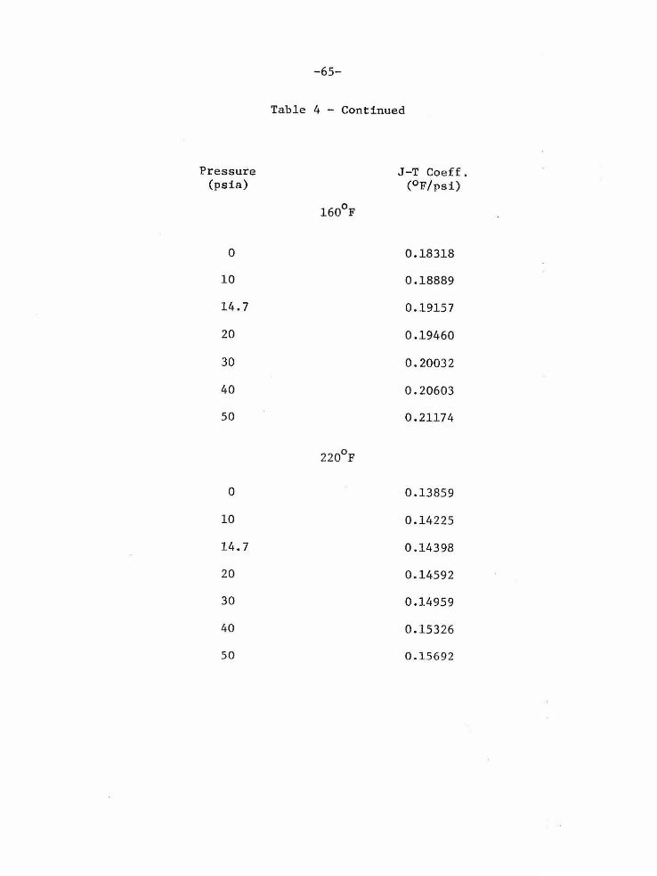
-65-

Table 4 - Continued

Pressure J-T Coeff. (psia) (OF/psi)

160°F

0 0 . 18318

10 0.18889

14.7 0.19157

20 0.19460

30 0.20032

40 0.20603

50 0.21174

220°F

0 0.13859

10 0.14225

14. 7 0 . 14398

20 0 . 14592

30 0.14959

40 0.15326

50 0.15692

-06-

Table 4 - Continued

Pressure J-T Coeff. (psia) (OF/psi)

280°F

0 0.10807

10 0.11047

14.7 0.11159

20 0 .11286

30 0.11525

40 0.11764

50 0.12003

TQmpe rature (OF)

100

160

no

280

100

100

160

220

280

µ

µ

µ

µ

µ

µ

µ

µ

µ

-67-

Table 5

EQUJ\TTONS FOR ISOTllEHMS

Equation

Propane

0.177823 + .287580 x l0-3P

0.131902 + .171090 x 10-3P

0.100888 + .108616 x l0-3P

0.079275 + . 072784 x l0-3P

n-Butane

0.256366 + .650011 x l0-3P + . 109282 x 10-4

0.256302 + . 65 2350 x l0-3P + .109061 x 10-4

0.183176 + .571298 x l0-3P

0.138586 + .366743 x l0-3P

0.108074 + .239157 x 10-3p

where µ is expressed in units of °F/psi and P in psia.

p2

p2

-68-

Table 6

CALCULATED VALUES OF THE JOULE- THOMSON COEFFICIENT AT ZERO PRESSURE FROM THE EQUATION OF FRANCIS AND LUCKHURST

Equivalent Experimental

Tc~mper at ure Cale. Value Value (OF) (°F/psi) (°F/psi)

Propane

100 0.18046 0.17782

160 0.13326 0 . 13190

220 0.10192 0 . 10089

280 0.08020 0.07928

n-Butane

100 0.26390 0 .25630

160 0.18854 0.18318

220 0.14073 0 .13859

280 0.10872 0.10807

-69-

Table 7

C.t\.LCULATED VALUES OF THE JOULE-THOMSON COEFFICIENT FROM THE BENEDICT-WEJm-RUJHN EQU.t\.TION

Pressure (psia ) 100°F 160°F 220°F

Propane

0 . 2064 .1491 .1115

10 .2079 . 1499 .1120

20 .2095 .1507 .1125

30 .2112 .1516 .1129

40 .2130 .1525 .1134

50 .2148 .1534 .1139

60 .2168 .1544 .1144

70 .2188 .1554 .1150

n -Butane

0 .2805 .2014 .1499

10 . 285 7 .2040 .1513

20 . 2913 .2069 .1529

30 . 2975 .2099 .1544

40 .3044 .2131 . 1561

50 .3120 .2166 .1579

280°F

.0859

.0862

.0865

.0867

.0870

.0873

.0876

. 0879

.1150

.1158

.1166

. 1175

.1184

.1194

-70-

Table 8

LABORATORY INSTRUMENTS

Thennocouple measurements

L&N Wenne r Potentiometer, Catalog #7559 (Ser. No. 1121093 or Chem. Eng. #20805)

L&N Galvanometer (Ser. No. 81108 or Chem. Eng. 111254)

L&N Standard Cell, Catalog #100, 1.01923 volts at 24°c (Ser. No. 768102 or Chem. Eng. #22582)

Platinum resistance thermometer measurements

Temperature measurements

Honeywell Rubicon Resistance Bridge (Ser. No. B-879 or Chem. Eng. #22687)

L&N Galvanometer, Catalog #2285-B (Ser. No. 1600861 or Chem. Eng. #22719)

L&N Platinum Resistance Thermometer, Catalog #8163 (Ser. No. 165026 or Chem. Eng. #23446)

Temperature control

L&N Resistance Bridge, Catalog #8067 (Ser. No. 1188897 or Chem. Eng. #20866)

L&N Galvanometer, Cata log #2285-B (Ser. No. 1165026 or Chem. Eng. #20845)

Caltech Platinum Resistance Thermometer (Ser. No. 1 or Chem. Eng. #1033)

Temperature calibration

L&N Platinum Resistance Thermometer, Catalog #8163 (Ser. No. 676711 or Chem. Eng. #20121)

Miscellaneous Caltech Designed Instruments

Oil Bath Chem. Eng. Drawing #27015-XL

Thyratron Modulator Chem. Eng. Drawing #26533-L

Temperature (OC)

26.286

%.259

37.716

37. 725

54.304

71. 083

71. 731

86.172

104.383

104.387

121.975

137.640

137.647

0.0

20.0

40.0

60.0

:'<

- 71-

Table 9

* Kl~Sl!LTS OF TllERMOCOlll'l.E CALlHl{J\T ION

Thermocouple A Thermocouple B (microvolts) (microvolts)

1048 . 70 1048 . 60

1062. 35 1062.50

1523 .40 1523.7()

1523.70 1523.90

2232.30 2232.40

2971.60 2971. 70

3001.00 3()01.00

3656.10 3656.10

4504.40 4504.20

4504.00 4504.90

5345. 70 5345.30

6112. 80 6112 .60

6113. 60 6113 . 10

Curve-Fit (microvolts)

1048.65

1062.44

1523.55

1523.83

2?.32.36

2971.95

3001.02

3655.90

4503.92

4504 .11

5345.61

6112. 74

6113 .12

0 .00

792.30

1692.80

2480.92

The above results must be multiplied by 3 for use with the thermo-couple ·networks of the calorimeter.

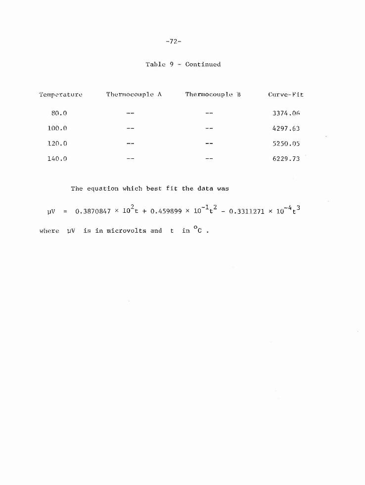
Temperature

80.0

100.0

120.0

140.0

-72-

Table 9 - Continued

Thermocouple A Thermocouple n

The equation which best fit the data was

Curve-Fit.

3371+.0h

4297.63

5250 .05

6229.73

µV 0.3870847 x 102

t + 0 . 459899 x l0-1t

2 - 0.3311271 x l0-4 t 3

where µV is in microvolts and t in °c .

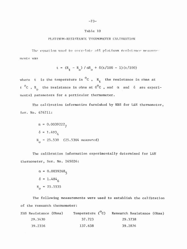
-73-

Table 10

Pl./\TINUM-Rl':SISTANl.E Tl!ERMOMETEH CAl .. TRRATION

Till' equat l\ln 11 :~ t·d l:u (:d1.·1·1• I at:,• ;1.l 1. pL1t: I lllllll rcHJ~:l ;1 111· t• 11u ·a~·: t11··· ·

mcnt:s was

t (R - R ) I a.R + cS(t/100 - 1) (t/100) t 0 0

where t is the temperature in °c , Rt the resistance in ohms at

t 0 c , R the resistance in ohms at 0°C , and a. and cS are experi­o

mental parameters for a particular thermometer.

The calibration information furnished by NBS for L&N thermometer,

Ser. No. 676711:

a. 0.00392227

cS l.493lf

R 25.530 (25.5304 measured) 0

The calibration information experimentally determined for L&N

thermometer, Ser. No. 165026:

a 0.00392685

cS 1.4846

R 25.5535 0

The following measurements were used to establish the calibration

of the r esearch thermometer:

NBS Resistance (Ohms)

29 . 3430

39.2356

T ( oC) emperature

37. 723

137.638

Research Resistance (Ohms)

29 .3738

39.2876

-74-

Table 10 - Continued

The following resistance measurements were used to check the

accuracy of the calibration:

NBS Resistance

Calculated Temperature

Research Resistance

Calculated Temperature

32.6956

71. 248259

32.7334

71. 248212

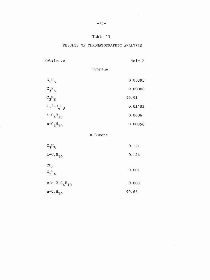
-75-

Table 11

RESULTS OF CHROMATOGRAPHIC ANALYSIS

Substance Mole '.%

Propane

C2H6 0.00395

C3H6 0.00008

C3H8 99.91

l,3-C4

H8 0.01483

i-C4Hl0 0.0606

n-C4

H10 0.00858

n-Butane

C3H8 0.191

i-C4Hl0 0.144

CH4 0.001

C2H4

cis-2-C4

H10 0.003

n-C4Hl0 99.66

-76-

Table 12

COMPARISON OF JOULE- THOMSON VALUES OF PREVIOUS STUDY CORRECTED FOR THERMAL TRANSFER WITH VALUES OF THIS STUDY

FOR n-BUTANE

The thennal-transfer correction applied was

CQ 1. 79 µ/P

where µ is the previous Joule-Thomson coefficient and P the absolute

pressure.

Pressure (psia)

14.7

20 .0

40. 0

14 .7

20.0

40.0

Previous J-T Coefficient

(°F /psi)

0.2343

0.2486

0.3012

0.1708

0 . 1772

0.1988

Thermally Corre cted J-T Coefficient

Value of this Study Deviation (°F /psi) (°F/psi) (%)

l00°F 0.2628 0.2682 -2 .00

0 .2708 0.2727 - 1.06

0.3146 0.2998 4.93

160°F

0 .1916 0.1916 0 .00

0.1931 0 . 1946 -0.87

0 . 2077 0.2060 0.82

220°F (t.T /b.P r atio uncorrected)

14.7 0 . 1173 0 .1316 0.1441 - 8 . 68

20.0 0. 1200 0 .1307 0.1459 -10.41

40.0 0 .1310 0 .1369 0 .1533 - 10.71

220°F (l:::.T/ t.P ratio corrected by a factor of 1.105)

14.7 0.1298 0. 1456 0.1441 1.ll

20 . 0 0.1327 0 . 1446 0 . 1459 -0. 88

40 .0 0.1448 0.1513 0.1533 -1.30

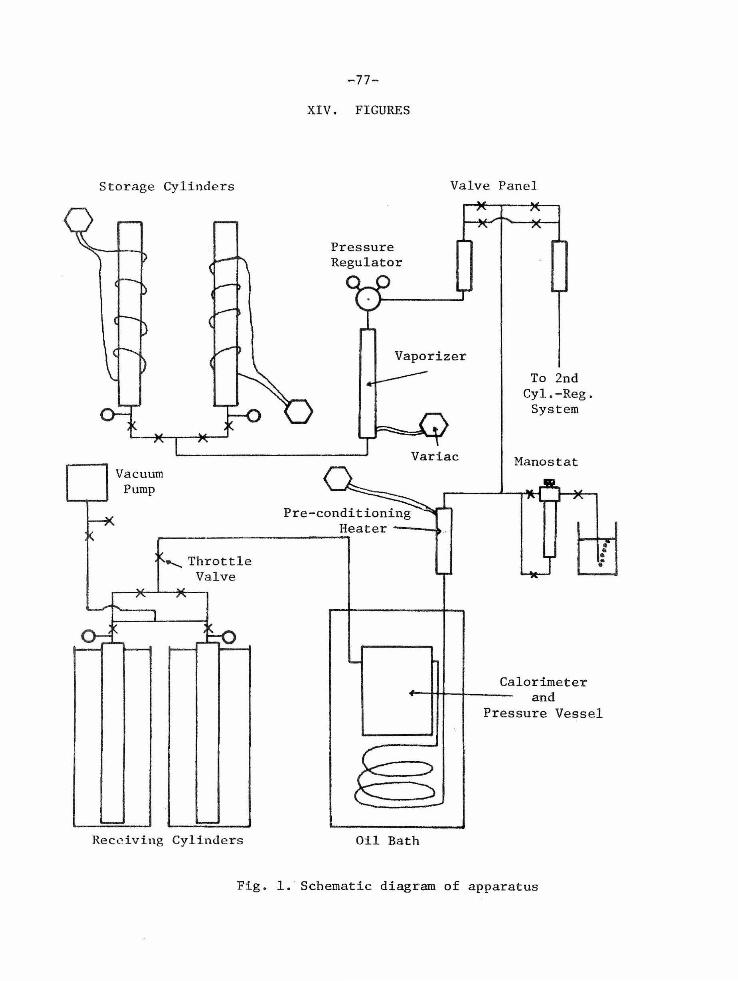
-77-

XIV. FIGURES

Storage Cylinders Valve Panel

Vacuum Pump

......_Throttle Valve

Pressure Regulator

Vaporizer

To 2nd Cyl.-Reg.

System

Manos tat

Calorimeter +--Hi+--+~~~ and

• • • .·

Pressure Vessel

Receiving Cylinders Oil Bath

Fig. 1. Schematic diagram of apparatus

Heat Shields

-78-

Thermocouples -- ·· ·;;.'I (every 120°) ·· '>-/' 4. O"--··--· - - .- · - -- ·-- 1~ - - -· . · -· ·1 ,,..-· .,,, '

,,,.,_ . f .·

'Ii I

l ' I i I

I 11 I

J :1 !1

~ ii ;1

ii 11 :I II 'I I

II

it

--·· ~ _)

I• -- 2. 8" -- - - - - ________ _.,

I l

s .s. Screws

4 . 5"

I Porous 1

Re~!:~:~c~J

Fig. 2. Full-Scale Drawing of Calorimete r

-79-

Fig. 3. Photograph of calorimeter showing all c omponents

-80-

19 I /Ii I . I" IC I" I I' •;3H:)NI \ I It I 1 / 1 1 f 1 l 1 I t 1 ! f I 1 I 1 If I I 1 I 1 1 J 1 J 11' I I . I 1 I 1 l 1 1 1+I1 I 1 I 1 I 1 l 1 I 1 1 I' I 1 Ir t ' l 1 1 • \•I 1 l 1 \ 1 I•\' L1 \ ' I•

Fig. 4. Photograph of calorimeter with porous thimble installed

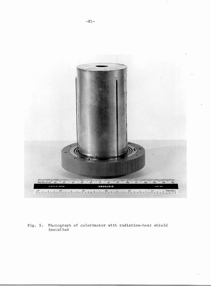
-81-

11111/1111/1111/1111/1111/lll llill// Ill II llT MCTIUCI CM 2 3 4

Fig. 5. Photograph of calorimeter with radiation-heat shield installed

Numbers represent the dimensionless-temperature, 0 = (T - T1

)/T2

- T1

)

0 0 0 0 0 0 0 . 5

Grid: 1/8-inch squares 0 I .CR] .060 .110 :llB5 .1~2 _53)0 11

0 0 0 0 0 0 0 I I I I I I ' .0$0 .1~2 .2to .340 A~O .?®o I 1

o I .EX)(f)3 .oe1 .002 .00'4 .oos -~o _QBo _ 110 _3f)o ~B 6ffio ?J:i,7 11

o I .LY'""~5 .0$2 .0$3 007 017 o-114 1'0 ~s :Wo ~o FAn fidn I 1

o I .0$1 .C~4 .008 .~7 .005 DPO .1:80 _2ffio 4Bo -~s "Alo AAA I 1

o I .0({)2 .(){)5 .ao ~o ffi5 ots r~n ~n ~~ ?ffio ~o qho 11

o 1 .utJ1 .<:Xf13 .o<p1 .Of 5 .o~o .oro .1t>O .540 .?l5 .~o .9©o .9!50 11

0 0 0 0 0 0 0 1 1 1 1

Radiation-Heat Shields ..;,. ...,.. ..,.. -"' ..r 1 Porous Thimble

Fig. 6. Dimensionless-temperature profile of the porous thimble mounting dis c

f if Exhaust

Gas

Center-Line of Exhaust Gas Exit Hole

I 00 N I

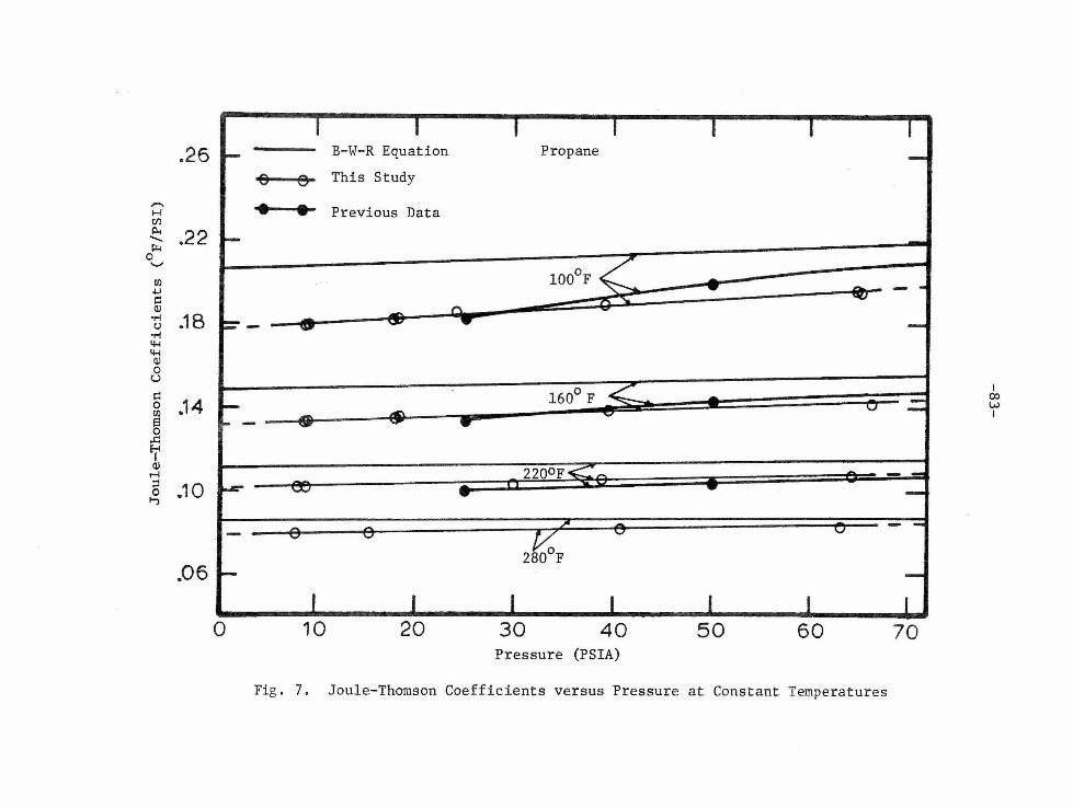
.26 t- B-W-R Equation Propane

e 0 This Study

,-... I • • H Previous Data u:i P-< .22 ........ ~

0 ...... Cl) I 100°F .µ i::: OJ

or! .18 (J

·r-i 4-{ 4-{

OJ 0 u i::: I= 160° F :;:.m =t I

.14 I 00 0 0 w Cl) - tC'I I 13 0

..c: er OJ .-l I ~ 2200F ;:l .10 0 ....,

.06

0 10 20 30 40 50 60 70 Pressure (PSIA)

Fig . 7. Joule-Thomson Coefficients versus Pressure at Constant Temperatures

,.-... ·rl

Cl) p.. -µ.,

0 .._, .µ i:: (l)

•rl (.)

-rl ~ ~ (l) 0 u i:: 0 Cl)

l::l 0 .c

E--< I (l) rl ;:J 0 .,

-84-

.20 Propane

.18

.16

,14

.10

0 0 50 Psia

• • 0 Psia

.06

.0 4

10 0 160 220 28 0 T ( OF) emperature

Fig . 8 . Joule-Thomson Coeffi cients vs Temperature at Constant Pre ssure s

.36

.32

.--.. ·ri Ill

p... .28 -µ. 0 '-'

en .IJ i:: <l)

.24 •M (.)

·M 4-1 4-1 <l)

0 u i:: .20 0 Ill s 0 .c H I

<l) r-1 .16 ::l 0 .....,

.12

.08

0

- 85-

n- Butane

160°F

B-W-R Equation

~o..,..~~o~ This Study

e e Previous Data

8 16 24

Pressure (Psia)

3 2 40 48

Fig . 9. Joule-Thomson Coefficients of n-Butane vs Pressure at Constant Temperature

-86-

' .30

n-Bu tane

.28

,,..... ·rt .24 Cl) p... -1%<

0 .._, .µ ~ .22 Q)

·rt C)

•rt 4-l 4-l Q)

0 u ~ .20 0 Cl)

s 0 .c H I Q) .18 r-1 ::l 0 .,

.16 • 40 Psia

0 20 Psia

.14 • 0 Psia

. 12

100 160 220 280 T t ( OF) empera ure

Fig. 10 . Joule- Thomson Coefficient vs Temperature at Constant Pressure

-87-

Propane

.24

,-.... •.-i Cl) p. .20 -Ii-< a '-'

.µ i:: Q)

•.-i .16 u

...... lH

~ lH Q)

~ a u i:: ~ a .12 ~ Cl)

13 a ,..c:: E-f I Q) rl

;::! .08 a .,

Eq. of Francis and Luckhurst

This Study

.04

100 160 220 280 T ( OF) emperature

Fig. 11. Comparison of Experimental Joule-Thomson Coefficients for Propane with Equation of Francis and Luckhurst at Zero Pressure

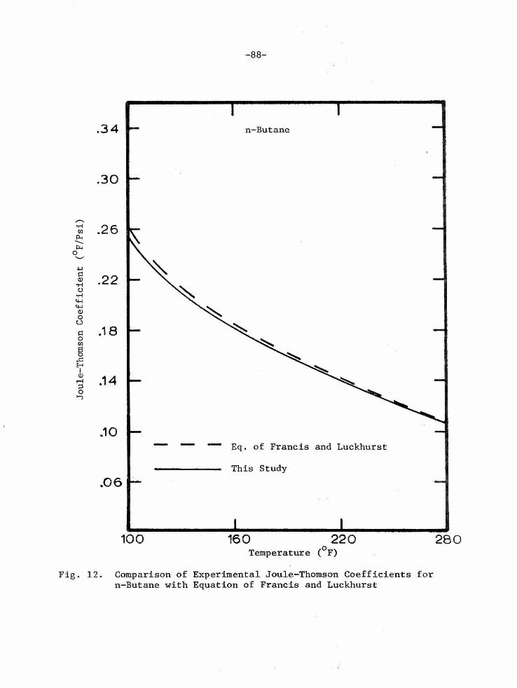
-88-

.34 n-Butane

.30

,,....._ ·rl .26 Cl) p.. -~ 0 .......,

.µ p

.22 Q) ~ (.) ~ •rl

4-4 4-4

~ Q) 0 u

~ p .18 0

~ (I)

g ~ ..c:

H ~ I

Q)

.14 ~ ::l 0 .,

.10 Eq. of Francis and Luckhurst

This Study

.06

100 160 220 T (OF) emperature

Fig. 12 . Compa rison of Experimental Joule-Thomson Coefficients for n-But ane with Equation of Francis and Luckhurst

280

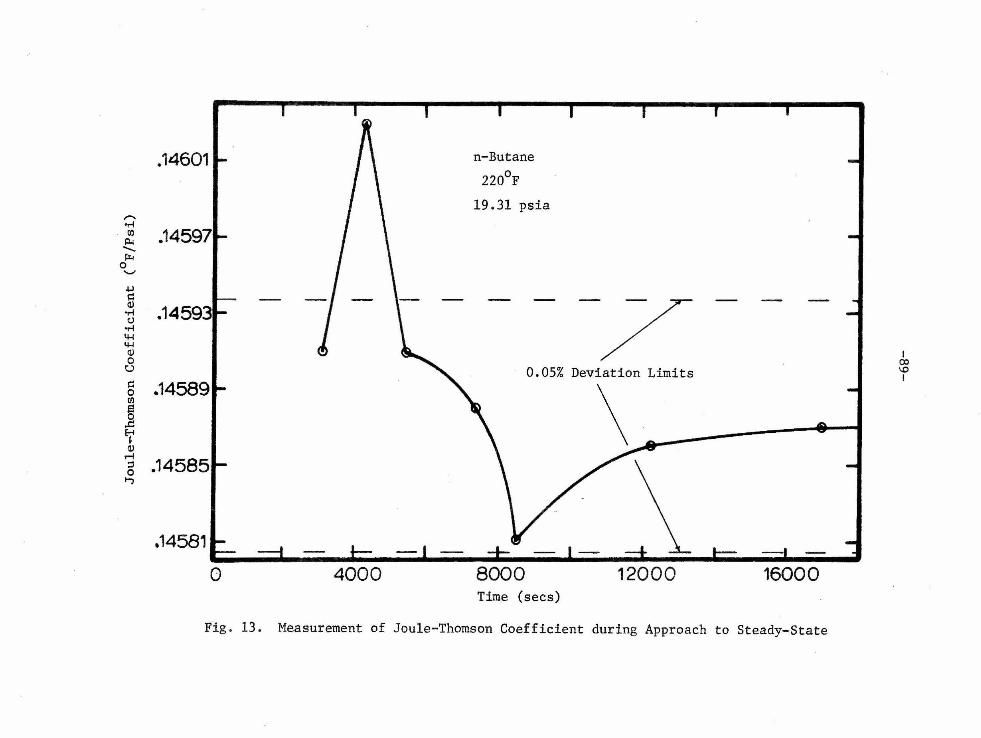
.14601 I- I \ n-Butane

220°F

19.31 psia -,..... -.-1 ti) .14597 ~ -µ:.,

0 '-'

.µ i:: Q) -

J - -

"8 . • 14593 - - - -7 -.-1

4-1 4-1 <1) 0 u I I

i:: .14589 0.05% Deviation Limits

co

0

'° ti) \

I

a ] )4 (IJ

r-f ::I .14585 0 ...,

.14581

0 4000 8000 12000 16000 Time (secs)

Fig . 13 . Measurement of Joule-Thomson Coefficient during Approach to Steady-State

-90-

.36 n-Butane

.32

0 10 20 30 40 Pressure (Psia)

Fig. 14. Compa rison of the Joule-Thomson Values of the Previ ous Study Corrected for Thermal Transfe r with Those of This Study

-91-

XV. APPENDICES

TEMPERATURE MEASUREMENT

All temperatures were measured by one or more of the following

instrwnents: mercury-in-glass thermometers, platinum-resistance ther-

mometers or thermocouples. Mercury-in-glass thermometers were used

for measurements where large errors in temperature would have a minor

effec t on the experimental results. These measurements consisted of

the room temperature, mercury-ma nome ter temperatures, resi s tance -hr i<lg<;

temperatures and barometer temperatures. Except in cases where the

thermometer was previously mounted on the equipment, the resistance

bridge for example, each mercury-in-glass thermometer was calibrated in

a water bath at 20, 25 and 30°C to the nearest 0.01°C.

A. PLATINUM-RESISTANCE THERMOMETERS

All absolute temperature measurements were taken with a platinum-

resistance thermomet e r (Chem. Eng. #23446). This thermometer was

purchased from Leeds and Northrup and calibrated for this study. Cali-

1~ration of the thermometer was based on the resistance versus tempera-

ture r e lationship of platinum as predicted by a modification of the

Callendar equation [55]. This temperature versus resistance relation-

ship was

where Rt

t ( (R - R ) I Cl.R ) + 0 (t/100 - 1) (t/100) t 0 0

and R are the resistances of the platinum resistor at 0

t 0 and o0 c, respectively. The two constants, a and o , are experi-

mental parameters for a particular platinum wire. Calibration

-92-

consisted of determining the ice-point resistance, R , plus the resis­o

tance at two additional temperatures. A second resistance thermometer

which had been calibrated by the National Bureau of Standards (Chem .

Eng. f/20121) was used to establish absolute temperatures during the

calibration. The same resistance bridge and oil bath used during the

calibration of the platinum thermometer we r e used for all measurements

of the experimental Joule-Thomson coefficient temperatures.

The procedure used to calibrate the platinum thermometer was as

follows. First, the ice points of the NBS-calibrated and the new

thermometer were measured. The thermometers were inserted into a

large Dewar flask that had been filled with distilled water and

crushed ice made from distilled water. The crushed ice extended to

the bottom of the flask and was stirred before each resistance meas-

urement . A series of resistance measurements was taken by each

thermometer with a Rubicon resistance bridge (Chem. Eng. #22687). A

plug board was used to switch from one thermometer to the other. The

ice-point resistance of each thermometer was read to the nearest

0 . 00005 ohm. The ice-point of the new thermometer was determined to

be 25.5535 ohms. The ice-point of the NBS-calibrated thermometer was

measured to be 25.5304 ohms which was in agreement with the ice-point

resistance of 25.530 ohms listed on its calibration card.

Next , both platinum-resistance thermomete rs were inserted into

the constant-temperature oil bath . A third platinum-resistance ther-

mometer (Chem . Eng. #1033) and a s e cond resist ance bridge (CheM . ~ng.

#20866), in conjunction with a thyratron modulator, were used to ma in-

tain the oil bath at the desire d t emperature during the resistance

-93-

measurements. After the bath temperature had been maintained at the

dt~ si red temperature hy the automatic feature of the thyratron modu] <Jtor

for about one hour, equ.ivalent manual settings were used and the

automatic feature was turned off. This was done to prevent fluctuatio11s

of temperature during the resistance measurements. When the oil bath

was controlled by manual settings, a slight drift usually developed.

This drift was checked and adjusted if necessary to be less than

0.0010-ohrn per hour prior to any measurement. Then a plot of resistance

versus time was made at 100 second intervals for both thermometers .

Usually a series of four to five resistances was taken with one ther-

mometer. Then the resistance bridge would be shifted to the other

thermometer and another series of resistance measurements would be

recorded. This procedure was continued until two series of resistances

were taken with the first thermometer and one series was taken with the

second. To obtain a resistance from each thermometer simultaneously,

it was necessary to extrapolate the series of resistance measurements

from one thermometer to a time corresponding to a resistance measure-

ment of the other thermometer. To minimize the extrapolation, a

common time very close to that of the switching from one thermometer

to the second was used. This procedure was used for three nominal

0 temperatures of 100, 160 and 280 F. These temperatures correspond to

those of tlw experimental measurements at each end of the measured

range and at one intermediate value. Using the measured resistances

from the NBS-calibrated thermometer, a temperature corresponding to

each measured resistance of the new thermometer was obtained. In this

manner Rt versus t°F was obtained for three temperatures. Since

-94-

there were only two unknown constants in the modifie d Callendar cqua-

tion other than the ice point which was previously measured , only two

of the three resistance measurements were needed for the calibration.

The 100 and 280°F resistance measurements were used. The t:hi.rd nwas -

urement at 160°F was used as a check on the calibratton and the

a greement was within O. OOOS°F. Other pertinent values recorded during

the cal ibration are g iven in Table 10.

At this point the relationship between temperature and resis-

tance are included to aid in the understanding of the limitations of

the me asurements . A change in r e sistance of 0.0001-ohm is approxi-

0 mat e ly equal to a temperature chan~e of 0.002 F. The resistance bridge

was r e ad directly to 0.0001-ohm and estimated to the nearest 0.00005-

ohm. The reading error was therefore 0.000025-ohm, representing a

tempe rature change of O.OOOS°F. This reading error is approximately

one-half the value normally given. The increased sensitivity of the

r esistance measurements was due, in part, to the increased distance

between the galvanometer and scale which measured the deflection. A

two-meter distance was used instead of the standard one-meter distance .

This added distance doubled the response of the galvanometer . The

reduce d light intensity required the galvanometer to be housed . All

galvanometers used in this study were operated at a two-meter distance .

Even though the calibration of the two thermometers agreed with

0 0.0005 F and the precision of the absolute temperature measurements of

0 the NBS-calibrated thermometer was better than 0.002 F, the accuracy of

the new thermometer is claimed to only 0.05°F in this study. This

discrepancy is due to the calibration of the resistance bridge . The

-95-

manufacturer of the bridge did not furnish a calibration card for the

changes in bridge-resistance readings due to changes in the bridge tern-

perature. The r esis tance coils were made of manganin. In the range

of room temperatures the resistance of manganin wire as a function of

temperature can be represented by [56)

0 0 2 R

25(1 - a(t - 25 C) - b(t - 25 C) )

The constants, a and b , in the above equation were determined from

an average of the constants of five 10-ohrn manganin coils wi t h NBS

calibrations. The values of the constants used f or this study were

a

b

The a bove resistance correction for bridge tempera ture changes was

applied to all resistance measurements. The magnitude of this c o r-

r ection ranged from 0 . 0 -ohm at 25°C to 0.0015-ohm a t 32°C and 40 ohms

total resistance. The above resistance curve compared favorably to a n

experimental curve determined for a similar resistance bridge. The

advantage o f using the above equation was in the writing of computer

programs .

Besides the resistance-bridge calibration for temperature

changes of the bridge, two other possible sources of error in the

resistance measurements were constantly checked. These sources were

the bridge zero adjustment and the bridge ratio adjustment. Bridge

temperature also affected these adjustments but the typical error was

0 u s u a lly less tha n 0.0002-ohm for a 3 to 4 C cha nge in r oom temper ature.

-96-

The platinum-resistance thermometer heating effect is a rosslblr• SOllrCl'

of error but was considered negligible due to the large volume of oil

in the bath. Therefore the claimed absolute temperature error of

O.OS°F which represents a resistance error of approximately 0.002.5-ohm

is thought to be conservative .

B. THERMOCOUPLES

Two thermocouple networks were used in this study to measure the

temperature change across the porous thimble. Each network consisted

of three thermocouples wired in series. All thermocouples used copper-

constantan junctions. (Actually "Advance" which is the Driver-Harris

Company tradename for constantan was used.) A precise calibration of

the thermocouple networks actually used in this study was not practi-

cal. The interior wires were only seven inches long and could not

reach from the oil bath to an adjacent ice bath. Therefore a segment

of wire was taken from each spool before and af ter the segment used for

the thermocouple networks. Two other thermocouples, labeled A and B ,

were made from these additional segments. The interior wires of A and

R were fourteen inches long. This additional length permitte d the

constant-temperature oil bath and platinum resistance thermometer of

the research apparatus to be used in the calibration. Using the resis-

tance thermometer to establish the temperatures, thermocouples A and B

were calibrated over the experimental range . Results of this calibra -

tion are listed in Table 9. The experimental points were fitt e d to a n

equation of the form

pV 2 3 at + bt + ct

-97-

where V is in microvolts and t in °c . Caltech Computing Center ' s

least-squares program was used to determine the constants a , b, and c .

The ;:ibove equation was recommended by NHS [57) for thl~rmocouplc calibra·­

t in11s. Both tht' I\ and B thcnnoconplt~s had essc-ntLd ly the same

standard deviation to the curve-fittc~d equation . Therefore it \./il~>

assumed that the thermocouple networks used in this study had similar

calibrations . The results listed in Table 9 are for one thermocouple

and must be multiplied by three to correspond to the networks used in

this study . The largest difference between the least-squares curve and

any experimental point was 0 . 48 microvolts in 4504 .4 total microvolts

or 0 . 012%. This difference was considered negligible, especially since

the temperature change was calculated from the slope of the calibration

curve.

On e Wenner potentiometer (Chem. Eng. 1120805) was used for all

thermocouple readings. This potentiome ter could be r ead directly to

0.1 microvolt and estimated to the nearest 0.05 microvolt. Since the

same potentiometer used in the calibration curve was also used for the

experimental measurements , any e rror resulting from the standard cell

would be reduced. The standard cell was checked by "bucking" it against

the standard cells of other potentiometers in the Laboratory . This

procedure indicated the standard cell to b e in excellent agreement wi t h

i ts calibration certificate. La borato r y records indicated the other

s t andard cells to he in agreement with their certificates.

The larg e st unknown value in the thermocouple measurements was

from parasitic EMF. No direct measurement of this EMF was obtaine d

s ince the the rmocouple networks c ould not be easily grounded. Estimate s

-98-

we r e made by the followi ng method . With no gas f lowin~~ throug h t h l'

calorimete r , thermocouple reading s were taken of the tempe rature chang e

a cross the porous thimble at the four isotherm temp e r a ture s . A zero

reading should have been measured at each temperature. Non- zero read-

ings we re attributed to para sitic EMF. In this manner the maximum

p a ras i tic EMF was determined to be less than 0.2 microvolt .

Error i n the me asurement of the temperature change used in the

calcula tion of the Joule-Thomson coefficient induce d an e rror in the

a b s olute t emperature of the coefficient, and vice versa . For ins t ance ,

the rmocouple readings from which the temperature changes were calcu-

late d had errors of up to 0 . 20 microvolt due to parasitic EMF, 0 . 05

microvolt due to inaccuracies in reading the potentiome t e r, and 0.05

microvolt due to the thermocouple calibration for a total of 0 . 30

microvolt . This 0 . 30 microvolt would correspond t o a maximum error

of 0 . 0042°F in the temperature change. An error of 0 . 0042° F in the

t empe rature change would induce an additional error of 0 . 0021°F in the

g as t empe rature. This 0 . 0021°F, when combined with the previously

esti.ma ted error of 0.05°F in the temperature due to r e sista nce the rmo-

me t e r inaccuracies , would result in a possible e rror of O. OS2°F . Since

the t empe rature of the gas was used to enter the thermocouple calibr a-

t ion cur ve , it would likewise induce an error in the me asured

temperature change . An error

cause a maximum error of only

of O.OS2°F in the gas temperatu re would

-6 0 5 x 10 F per microvol t in the t empera-

ture change. Since the largest thermocouple reading was less than

130 microvolts, this latter error was neglected .

- 99-

APPENDIX II

PRESSURE MEASUREMENTS

All pressure measurements were made with one or more of the

following instruments: mercury barometer, mercury manometer, pressure­

balance system [40,58] and high-pressure manometer [59] .

Atmospheric pressure was mea sured with a brass-tube mercury

barometer. Corrections to the barometric pressure were made for tem­

pl~rn tu rc [(iO], g ravity in Pasad t>nn, and elevation diffprc ncc!s br~ t.wer:n

t:lll' harometcr and ap paratus. Pressure measure ments were r ecorded to

the neares t 0.01 mm Hg . The accuracy of the atmospheric p r essure was

estimated to be ±0 . 1 mm Hg b e cause of reading and adjustment errors .

The pressure of the gas, prior to being throttled, was measured

either by a mercury manometer which had one leg open t o the atmosphere

or by the pressure-balance system. Both instruments relied on the

barome tric pressure for absolute values of the pressur e. The mercury

manome ter was read by a cathetometer to the neares t 0 . 01 mm Hg . necause

of mercury curvature a nd cath e tome ter inacc uracies , the accuracy of

t lie me r cury manometer readings was e stjmated to be ±0.05 nun Hg. The

pressure-bal ance system was use d when the pre ssure exceeded t wo atmos­

pheres gau g e . Pressures from t h e pressure-balance system were read to

the neares t 0 . 05 psi. Due to changes in the density of the oil line

b e t ween the mercury trap and balance, the press ure measurements were

estimat e d to have an accuracy of 0.1 psi . Therefore the maximum error

in the absolut e pressure would be a pproximately 0 . 1 psi.

-100-

The pressure change across the porous thimble was measured with

a differential mercury manometer and/or the high-pressure manometer.

The differential-mercury manometer was used for all pressure-change

measurements even though the high-pressure manometer was connected and

working. The primary advantages of the mercury manometer were its

higher accuracy (0.05 mm Hg to 0 . 3 mm Hg), speed in obtaining a pres­

sure, and constant visual indication . Its max imum working pressure

was 100 psi . All measurements of the pressure change were correc t ed

for temperature, gas densities in the manometer and Pasadena gravity .

The error in the absolute pressure induced by e rror in the

pressure change was small and therefore neglected.

-101-

P R 0 P 0 S I T I 0 N S

-102-

PROPOSITION I

The me thod of oxidation-reduction cycl:l.ng as us e d in the prep­

aration of metal powders by Czan<lerna [l] is propose d for the rcmova .1

of oxidation products and undesirable discoloration from the surf aces

of rare coins. An easily constructed reactor is described in which to

carry out the reactions.

INTRODUCTION

The present-day art of rare coin cleaning leaves much to be

desired. Corrunercial and homemade cleaners consist primarily of liquid

acids or abrasive pastes which remove a fraction of the metal surface

during the cleaning process. A uniformly-cleaned surface with these

cleane rs is difficult to obtain without the removal of an excessive

amount of metal due to crevices in the design and also lettering on a

coin. Coins cleaned in liquid acids have a tendency to corrode or

change to an abnonnal color, e.g., grey copper.

The r emoval of metal from the surface of a coin, either by

wear or chemical action, reduces its value significantly. For example,

an uncircula ted coin of a particular date is generally 25 to SO percent

more valuable than an almost uncirculated coin. An old coin with an

attractive appe arance is treasured by collectors and sold at premium

prices b y coin dealers. Since copper coins have the greatest t endency

to chemically change to an undesirable color, the oxidation-reduc tion

cycling method was tested with copper coins. The method is applicable

for all me tallic coins even though not specifically tested.

-103-

The proposed oxidation-reduction cycling method offers a metho d

of cleaning discolored coins without chemical or mechanical damage . The

me thod is more difficult and less economic al than liq11id cl e an:l.ng i f

c oi.n damag e l s not considere d. Commercial clt>ane rs rangl.' in cos l rrom

about $2.50 for one -st e p cleaners to $30.00 for a rnulti-st e p cl e aning

process consisting of six to e ight different liquids. There are many

coins valued above $2000 ( 2 ) and some have been sold at auctions at

prices up to $47,000. The slightly higher cost of the oxidation­

reduction process is not of great concern provided the method enhances

rather than decreases the value of the co i ns.

THEORY

The proposed oxidation-reduction cycling me thod consists of

repeated exposure of the coins to pure oxygen at a constant elevated

temperature, followed by chemical reduction with hydrogen at approxi-

mately the same temperature. Typical reactions which might occur

during the oxidation and reduction steps are:

Oxidation

2 Cu + 2 CuO

> n co2 + (n+l) H20

Reduction

>

The removal of undesirable surf ace colors without the removal of metal

is the primary b enefit of the oxidation-reduction cycling process.

The possibility of a spontaneous reaction between hydrogen and

oxygen was considered. If h ydrogen comes into contact with oxygen

only at room temperature and atraospheric pressure and the reactor tern-

perature is kept below 500°c, the possibility of a spontaneous

reaction is negligible. A good reference on the hydrogen-oxygen

reaction is given by Pease [3].

-105-

EQUIPMENT

The oxidation-reduction cycling reactions were carried out in

the apparatus illustrated in Figure 1. The reactor consists of a

4-foot length of Pyrex tubing with an inside-diameter of 9 mm. A

400-watt tape heater, coiled around the exterior of the Pyrex tube,

supplied the energy to increase the reaction rates . Temperature of the

reactor was manually controlled by a Variac. Giass wool surrounded the

heater to prevent excessive heat losses to che environment. Rubber

scoppers were used to seal the ends of the reactor. Hydrogen and

oxygen entered and exited the reactor by 1/ 4-inch copper tubing which

was inserted through a hole in each stopper. A mercury thermometer

with a range of -10 to 4oo0 c was placed tnside the reactor ·to measure

the reaction temperature. Glass wool, wrapped around the thermometer,

prevented direct contact between the thermometer and walls of the

reactor.

Large thermal gradients occurred in the axial direction in the ·

reactor because the temperature of the inlet gas was ~ncreased as it

flowed through the heated section. The oxidation-reductio~ reaction

was carried out at the hottest location in the reactor which was at the

downstream end of the tape heater. The bulb of the mercury thermometer

was located in the hottest section. Even when the reactor was operated

0 at a temperature of 450 C, the ends of the reactor remained near room

temperature due to the small heat capacity of the gases.

After pas sing through the reactor, the exhaust gas was bubbled

through a beaker filled with water. The bubbling process prevented

-106-

air from leaking into the reactor and helped indicate the flow rate of

the oxidizing or r educing gas. The reactor was located in the hood for

the purpose of disposing the exhausted hydrogen or oxygen. Safety

plate g lass on the front of the hood provided protec tion in the event

of an explosive reaction between hydrogen and oxygen.

High-pressure storage cylinders served as a source of the

reactant gases. Gas pressure was reduced to 10 psig at the cylinder

regulator. A flame arrester and throttle valve after the regulator

further r e duced the pressure so that the gas pressure in the reactor

was approx imately 3 inches of water above atmospheric. A rotameter in

the inlet gas line was used to me asure the flow rate .

-107-

CLEANING PROCEDURE

Prior to placing the coins into the reactor, all foreign material

not chemically attached to the surface was removed in an ultrasonic

cleaner using soapy water. The coins were then rinsed in distilled water

and air dried . Then they were placed on glass wool and inserted into

the reactor. Room temperature oxygen from the storage cylinder initially

flowed through the reactor at a rate of 20 ft3/hr to flush the air.

After a two-minute flushing period, the oxygen flow was reduced to

1 ft 3/hr and the Variac controlling the heater was set for a reactor

0 temperature of 300 C in the reaction zone. The initial oxidation cycle

lasted 30 minutes at 300°c and each subsequent oxidation cycle was

increased by an additional thirty minutes until the coins were clean.

Each oxidation cycle was followed by a hydrogen reduction cycle. The

total number of oxidation and reduction cycles depended on the original

condition of the coin. Three to four complete cycles were typical.

Following the oxidation cycle, the heater was turned off with

oxygen continuing to flow through the reactor. When the reactor tempera-

0 ture cooled to b e low 60 C, the oxygen flow was stopped and the oxygen

cylinder replaced with a hydrogen cylinder. Similarly, room temperature

3 hydrogen initially flowed through the reactor at 20 ft /hr to flush the

remaining oxygen from the reactor. Then the heater Variac was set for a

reactor temperature of 325°C. The duration of each reduction cycle was

approximately the same length of time as the preceding oxidation cycle .

Observation of the coin through the glass reactor made possible the

shortening of the reduction cycle at times. After the reduction cycle,

-108-

the heater was turned off while hydrogen continued to flow in the same

manner as the oxidation cycle. 0 Upon cooling to below 50 C, the coins

were removed from the reactor and inspected with a microscope . The

condition of the coins determined if further oxidation-reduction cycl-

ing was needed .

-109-

RESULTS AND CONCLUSIONS

Photographs illustrating the results of liquid cleaning and the

oxidation-reduction cycling method are given in Figures 2a through 2d.

All photographs were taken with 48-power magnification and show only a

small portion of the . flat surface of various copper pennies. Figure 2a

shows the typical surface of a newly-minted penny. Figure 2b illus­

trates the removal of metal by liquid cleaners when used according to

the instructions. The top half of this penny was protected from the

cleaner with grease during cleaning. Figure 2c indicates what can happen

to the surface of a coin when one tries to do a thorough job around the

lettering. The surface was highly etched. Figure 2d i llustrates the

surface of a penny after having undergone three complete oxidation­

reduction cycles . The penny was initially oxidized to the typical brown

color through normal circulation. The lines in the photograph are from

scratches due to circulation rather than the cleaning process.

The oxidation of copper coins and subsequent reduction with hot

hydrogen proved to be a successful method of removing oxidation

products from the surface without damage to the coins. · The oxidation­

reduction process is more uniform than most liquid cleaners as gases

penetrate the crevices in the design better than liquids. Unlike

liquid cleaners which remove a small amount of metal each time, the

cycling process can be used repeatedly without damage to the coin.

The proposed process ,is slower but several coins can be cleaned simul­

taneously . Disadvantages i nclude the obtaining and setting up of the

apparatus and the strict adherence to safety precautions when mixing

-110-

hydrogen and oxygen. A larger reactor would be ne cessary for coins

having a diameter larger than 9 mm.

Long range effects of the oxidation-reduction process were not

observed. Prior to cleaning any valuable coins, the tendency for

cleaned coins to corrode or reoxidize to an undesirable color should be

observed.

Coins can be ruined if the reactions take place at too high a

temperature. To prevent distortion of the coins, do not heat them

above the recrystallization temperature, which for pure metals is

approximately 40% of the absolute melting temperature [4]. The

recrystallization temperature for copper is approx imately 370°c [SJ.

One experimental cleaning cycle at 4S0°C resulted in poorly cleaned

coins with severely etched surfaces. An extremely thin layer of copper

peeled off three different pennies. A silver dime also in the reactor

became copper colored. The metallic ions apparently became highly

mobile at the higher temperature.

Another point to consider before cleaning coins by any me thod

is the desi red final color . Coins cleaned with the oxidation-reduct ion

met hod had a slight reddish- orange color rather than t he yellowish­

orange color of newly minted coins . Upon exposure to the atmosphere

for several day s , a slow change to the mint color was noticeable . Whe ther

coins over 100 years old should have the color of newly minted ones is

a matter of pe rsonal choice.

If the coin initially had an undesirable color, the oxidati on­

reduc t i on me thod would certainly improve its appearance.

-111-

REFERENCES

1. A. W. Czanderna, "Magnetic Susceptibility Changes in Silver Powders

During Oxidation-Reduction Cycling," J. Phys. Chem . 71, 1967,

pp. 770-771.

2. R. S. Yeoman, A Guide Book of United States Coins, 22nd Ed.,

Western Publishing Co., Racine, Wisconsin, 1966.

3 . R. N. Pease, B. Lewis and H. S. Taylor, Combustion Processes,

Princeton University Press, Princeton, 1956, pp. 160-174.

4. D. S. Clark and W. R. Varney, Physical Metallurgy for Engineers,

2nd Ed. , D. Van Nostrand Co., New York, 1966, p. 358.

5. W. A. Lange, Handbook of Chemistry, 10th Ed., McGraw-Hill, New

York, 1961, pp . 246-247.

Rubber Stopper

0 0 0

()Q

Beaker Filled with Water

Hg Thermometer

Tape-Heater

Glass Reactor

Variac

High-Pressure Storage Cylinder

Fig. 1. Drawing of Reactor

Rotameter

I 1--' 1--' N I

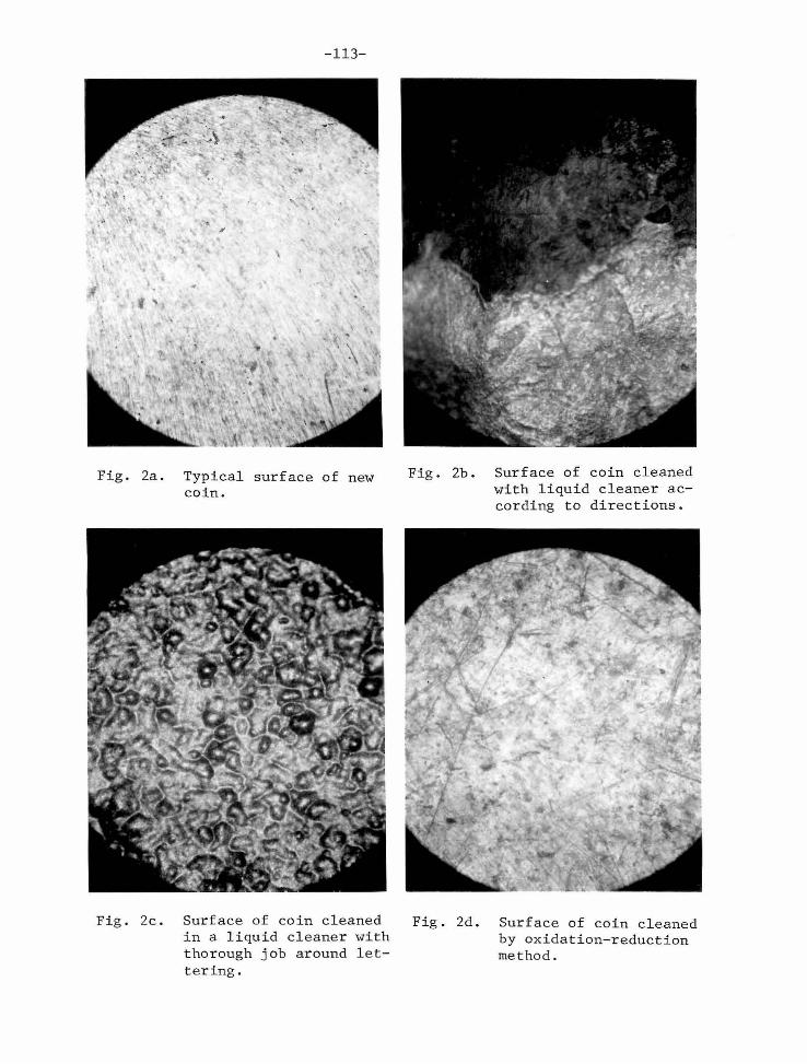
Fig. 2a.

Fig. 2c .

-113-

Typical surface of new coin.

Surface of coin cleaned in a liquid cleaner with thorough job around l et­tering.

Fig. 2b. Surface of coin cleaned with liquid cleaner ac­cording to directions.

Fig. 2d. Surface of coin cleaned by oxidation-reduction method.

-114-

PROPOSITION II

The galvanic response of a Hersch detector [l] is related to

the concentration of oxygen of a gas sample passing through it. By

varying the load-resistance of the cell, concentrations of oxygen from

0 to 50,000 ppm may be correlated with the output of a one-millivolt

recorder. An equation is proposed which relates the load-resistance

of the detector to the response of a millivolt recorder for a given

concentration of oxygen.

INTRODUCTION

A Hersch cell is a specific and sensitive detector of oxygen

which offers higher sensitivities than possible with other types of

oxygen detectors. It consists of a silver cathode and lead anode in

contact with an electrolyte containing hydroxide ions. A carrier gas

continuously flows through the cell. Oxygen in the carrier gas is

reduced at the cathode and an electric current is generated according

to the following electrode reactions:

Cathode

> 2 OH

Anode

Pb+ 3 OH - 2e-

Hersch cells are normally operated either with continuous

flow through the cel l of the gas to be analyzed, or with a "blank"

carrier gas and the oxygen-containing gas injected in pulses . For

-115-

cells operated in the continuous manner, mathematical equations relat­

ing current output to concentration of oxygen have been proposed (1,

2]. Since oxygen constantly flows through the cell, an ammeter can be

used to measure the current output.

When the Hersch cell is operated in the pulse manner; small

samples containing oxygen are injected into the carrier gas, similar

to the injection method of gas chromatography. Current output of the

cell varies according to the concentration of oxygen within the cell .

Therefore the use of an ammeter is not feasible to measure the current

output, since it would be difficult to record the maximum or average

current. To measure the current a load-resistor is placed in the cir­

cuit of the Hersch detector and a millivolt recorder is used to

measure the voltage drop across the resistor. In this manner, a per­

manent record of the output of the cell can be obtained.

Concentrations of oxygen up to 50,000 ppm can be analyzed when

small samples are injected into the carrier gas. Since millivolt

recorders are somewhat limited in range, different resistors are used

to keep the voltage drop within the limits of the recorder. The value

of the resistor which is placed in the circuit of the Hersch cell

affects the current output of the cell. The effects of a resistor are

determined by calibrating the cell using pulses of known concentrati ons

of oxygen. If several different resistors are used in the analysis of

widely-varying concentrations of oxygen, the present method of opera­

tion is to individually calibrate each resistor [3,4]. Since cell life

is difficult to determine except by actual service [5], the calibrations

-116-

are normally repeated daily and sometimes more often for very accurate

studies. The proposed equation relating the output of a Hersch detec­

tor to load-resistance for a given concentration of oxygen will reduce

the amount of calibration data required to that for a single resistor .

-117-

THEORY

The purpose of this section is to relate the effects of the load

resistance to the electrical output of a Hersch detector for a given

concentration of oxygen. It was assumed that the Hersch cell could be

represented by a current source. The internal resistance of the current

source is in parallel to the load resistor. Hersch [l] implied a simi-

lar circuit for the continuous-flow detector. In addition, it was

postulated that the cell current is proportional to the partial pressure

of the oxygen at the cathode. This relationship can be stated mathe-

matically:

i (1)

where p02 is the partial pressure of the oxygen and k is the con-

stant of proportionality. For a particular cell operated at a

specified flow rate of the carrier gas, the partial pressure of the

oxygen is proportional to the concentration of oxygen in the injected

sample:

(2)

where c0

is the concentration of oxygen. Combining Equations (1) 2

and (2) yields

i (3)

where k2 = k k1 • The current produced by the cell is equal to the

voltage of the cell divided by the total resistance of the cell and

external circuit. Therefore Equation (3) can be restated:

E/R = tot (4)

-118-

where E is the cell voltage and Rtot the total resistance of the

cell. The total resistance is related to the inte rnal resistance and

load resistor by:

(l/R + l/p) (1 + R/p) I R ( 5)

where R is the load resistor and p the internal resistance of the

cell. Combining Equations (4) and (5) yields

E = k2 co R I (1 + R/p) 2

(6)

The peak height, H , of the millivolt recorder is a linear function of

the cell voltage and this relationship can be expressed:

(7)

Combining Equations (6) and (7), the proposed equation relating the

response of a millivolt recorder to load-resistance for a g iven oxygen

concentration is obtained:

H k4

c0

RI (1 + R/p) 2

(8)

where k4 = k 2 k3 • The constant, k4 , is not a true constant, since

it is a function of the flow rate of the c,arrier gas, Hersch cell

design, and cell efficiency. For a given cell and flow rate, it does

remain constant provided the efficiency of the cell does not change.

The value of k4 is obtained by calibrating the cell with oxygen

samples of known concentration. Even when the day-to-day efficiencies

of the cell vary, new values of k4 can be obtained by r ecalibrating

the ce ll frequently.

-119-

The values of k4

and p were obtained by simultaneously

solving Equation (8) using the data of the 1 and 1000-ohm resistors

listed in Table 1. In particular, values of the slopes of the peak

he i ght versus oxygen concentration for the 1 and 1000-ohm resistors

we.re 7.03 x 10-5 and 3 . 04 x 10-2 mv/ppm, respectively. Usi ng

these data, the values of k4 and p were determined to be 7 .04 x 10-5

mv/ohm-ppm and 760 ohms, respectively. Inserting these values into

Equation (8) yields

H = 7 .04 x 10-5 c0

R/ (1 + R/760) 2

(9)

Equation (9) is applicable only for the particular cell used to obtain

the data listed in Table 1. Since the data of only two of the seven

resistors were used to obtain Equation (9), a good correlation with the

remaining five resistors would substantially support the proposed

equation.

-120-

EXPERIMENT

The data listed in Table 1 were experimentally determined by

Blakemore [6]. A Hersch cell similar to the design of Phillips [4] was

used in the measurements. The relationship between oxygen concentra­

tion and recorder output was determined for seven different resistors:

1, 3, 10, 30, 100, 300 and 1000 ohms. Eight primary gas mixtures,

ranging from 20 to 37,390 ppm of oxygen in argon, were used for the

calibration. Each of the eight primary samples were further diluted

with argon to yield a larger variation in the concentration of oxygen .

Sample volumes of 0.2 cc were injected into the argon carrier gas

which flowed through the cell at the rate of 20 cc/min. Ninety-five

percent of the data were estimated to have an error of less than 5%.

-121-

RESULTS AND CONCLUSIONS

The proposed equation which relates the load resistance of a

Hersch detector to the response of a millivolt recorder for a given

concentration of oxygen is

H k4

c0

R/(l+R/p) 2

(8)

where the constant, k4

, and internal cell resistance, p , are functions

of a particular Hersch cell. For the cell and operating conditions used

to determine the data listed in Table 1, values of k4

and p were

calculated to be -5 7.04 x 10 mv/ohm-ppm and 760 ohms , respectively .

Inserting these values into Equation (8) yields

H = 7.04 x 10-5 c0

R/ (1 + R/760) 2

(9)

Equation (9) was used to calculate the peak height of the millivolt

recorder as a function of the concentration of oxygen for the seven

different resistors listed in Table 1 . The results of these cal cula-

tions are represented by the solid lines in Figures 1 and 2 . The

experimental data listed in Table 1 were also plotted in the se figures

in order to compare the results.

The agreement between the calculated values and the experi-

mental values is well within the experimental error of the data. The

poorest agreement resulted from the data of the 3-ohm resistor. The

direction of the disagreement could be explained by a loss in cell

efficiency. Since the data of each resistor does agree wi th the

calculated values, the proposed equation would reduce the amount of

-122-

calibration data required for this particular cell. The more general

expression, Equation (8), should apply to all cells of similar con­

struction.

-123-

REFERENCES

1. P. A. Hers ch, "Trace Monitoring in Gases Using Galvanic Systems , "

Analytical Chemistry 32, 1960, pp. 1030-1040 .

2. Advances in Analytical Chemistry and Instrumentation III, Wiley,

New York, 1964, p. 219.

3. G. E . Hillman and J. Lightwood, "Determination of Small Amounts of

Oxygen Using a Hersch Cell as a Gas Chromatography Detector ,"

Analytical Chemistry 38, 1966, pp. 1430-1433;

4 . T. R. Phillips, E. G. Johnson, and H. Woodward, "The Use of a Hersch

Cell as a Detector in Gas Chromatography," Analytical Chemistry

]&_, 1964, pp. 450-452.

5 . W. J. Baker, J . F. Combs, T. L. Zinn, A. W. Wotring and R. F. Wall ,

"The Galvanic Cell Oxygen Analyzer," Industrial and Engineering

Chemistry 51, 1959, pp. 727- 730.

6 . J. E. Blakemore, personal conununications, 1970.

cc

H

i

k, k1

, etc.

mv

R

R tot

p

-124-

NOTATION

cubic centimeters

concentration of oxygen in ppm

voltage of cell

peak height of millivolt recorder in millivolts

current of cell

constants of proportionality

millivolts

partial pressure of oxygen

parts per million by volume

load-resistor in ohms

total resistance of cell

internal resistance of cell

-125-

TABLE 1

EXPERIMENTAL HERSCH-CELL DATA

Resistance Oxygen Concentration Peak Height (Ohms) (ppm) (mv)

1000 180 5 . 04

1000 138 4.26

1000 137. 5 4.37

1000 140.S 4 . 35

1000 74.7 2.55

1000 73.7 2 . 39

300 20 .311

100 117 .3 . 725

100 47.2 .319

100 135.5 .794

30 180 .386

30 117.3 .254

30 326 .656

30 398 . 717

30 172 .356

30 180 . 375

30 135.5 .274

Resistance (Ohms)

10

10

10

10

10

10

10

3

3

3

3

3

1

1

1

-126-

TABLE 1 - Continued

Oxygen Concentration (ppm)

770

540

326

940

600

398

1200

3890

3080

2520

2010

1200

8260

5620

3140

Peak Height Cmv)

. 556

.377

. 229

.653

. 412

.247

.824

.782

.626

.510

.404

.240

. 580

.395

.218

1

o~ T 1 • : I • I I 1 0 300 600 900

Oxygen Concentration (PPM)

Fig . 1 . Oxygen Concentration vs Peak-Height for Five Different Resistors

.6

.5

,-,. Cl) .µ

.4 r-1 0 >

or-f r-1 r-1 or! 13 ........ .µ

•3f I / 1 I ,.c: f-'

N bO 00 or-f I Q) • 3 ohms ::i:: ,.!<l

~ . • 2~ I /- 0 1 ohm

Calculated Values

I I / .1

OK I I I I I I I I I •

0 3000 6000 9000 Oxygen Concentration (PPM)

Fig . 2. Oxygen Concentration vs Peak-Height f or Two Resistors

-129-

PROPOSITION III

A design for a rotameter which can be used as a viscometer is

proposed. Design features significantly increase the normally unde­

sirable viscosity dependence of a standard rotameter. Mathematical

equations describe the viscosity relative to the position of the float .

INTRODUCTION

Since the 1940's rotameters have become increasingly important

in the measurement of flow rates of fluids. Design work has been pri­

marily in the area of reducing the dependence of the flow rate on

fluid properties [l,2,3]. In this study a rotameter has been designed

to take advantage of the viscosity dependence in order that it might

be used as a viscometer. Advantages of the proposed viscometer are

its ability to monitor the viscosity of continuous-flow processes while

maintaining simplicity in design.

-130-

DISCUSSION

The proposed viscometer design is illustrated in Figure 1 .

Features which separate the proposed viscometer from typical rotameters

are: (1) a streamlined float which has its wall parallel to the tapered

glass tube, and (2) a small-diameter rod which maintains the float con-

centric with the glass tube.

The equation rela ting the position of t h e float to the viscos i ty

of the fluid was derived by making a steady-state, force balance on the

float. The force balance yields:

P' A' - P' A' - f P' sin e dA' = - T A" - V (1) 2 2 1 1 s s rz l s fpfgx

A' float s

pressure drag gravity

where:

A' 2

is the cross sectional area of the top of the float

A' 1 i s the cross sectional area of the bottom of the float

P' 2

is the pressure applied to A' 2

P' 1

is the pressure applied to A' 1

P ' is the pressure applied to A' s s

A' is the surface area of the sides of the float s

A" is the surf ace area of the entire float s

z is the coordinat e-direction parallel to the taper of the float

x is the coordinate in the vertical direction

T i s the momentum flux rz

-131-

vf is the volume of the float

pf i s the density of the float

gx is the component of gravity in the x direction

e is the angle between the x and z coordinate directions

An exact solution to the above equation would be difficult . If the

taper of the glass tube is limited to a small angle, Equation (1) can

be simplified by assuming that the wall of the tube and the float form

coaxial, right-circular cylinders at each float position (See Figure 2) .

Equation (1) then becomes :

-As Trxl - Vf fgx

r=kR

(2)

where kR is the ari thmetic average of the top and bottom radii of the

float , A12 the cross-sectional area of the float using radius kR ,

A the surface area on the sides of the float, and R the inside s

radius of the tube .

Equations describing the steady, laminar, Newtonian flow of an

i ncompressible fluid in the annulus of the above geometry have been

derived [4] and the results are:

(i)

< V > x

The average velocity

. 2 (P1 - P2)R ~-8n Lf 1 -

k4

k2 1 - k

2)

Q.n(l/k) (3)

where:

-132-

(ii) The volume rate of flow

Q

(iii)

T rx

p

Lf

n

R

TI(P ~ P )R4 1 2

The momentum flux

(P1

- P2

)R (i- [ 2Lf

is defined as p + p

is the length of the

1 - k2

2 Q.n(l/k)

gx

float

is the viscosity of the fluid

. ~)

is the inside radius of the outer, coaxial cylinder .

Substituting Equations (3), (4) and (5) into Equation (2) yields:

2 - Sn L Q [k -f

(1 - k2) 2 Q.n(l/k)]

A solution to Equation (6) is difficult to obtain since P' 1

and P' 2

are affected by the acceleration and deceleration of the

fluid at the ends of the float. To obtain values for P' 1

and

(4)

(5 )

(6)

it was assumed that the pressures acting on each end of the f 1oat are

equal to the corresponding pressures at each end of the annulus. This

assumption is crude but the errors which are introduced will be

similar at each float position. Calibrating the viscometer with a

-133-

fluid of known viscosity and determining all other viscosit i es relative

to the calibration will decrease the error.

If t h e pressure s at each end of the annulus, as dete rmined by

Equa t i on (4) , are used to replace

following result is obtained

P' 1

and P' 2

in Equation (6); the

_2 ___ 8n_:_L_f_(_1 ___ k_2_)_2_ (~~; - k2 + / i~(~;) R [(l - k) - in(l/k) ] ~ )

(7)

Since Vf is equal to the product of A12 and Lf , and since Rf is

equa l to kR, the above may be rearranged to yield:

1 - k2 2 n [ 2 in(l/k)] k

4 (1 - k2) 2 (l - k ) - i n(l/k)

( 8 )

The left-hand side of Equation (8) excluding the viscosity, n , i s sole l y

a function of the float position for a given viscometer, sin ce

where Rf is the radius of the f l oat and x the distance above t he poi n t

where the radius of the float and g lass tube are e qual. Equa t i on (8) can

be expressed :

nF(x ) = (9)

wh e r e

F(x)

-134-

4 (1 - k2) 2 ((l - k )- ~n(l/k) ]

For a given viscometer, it is possible to calculate the viscosity from

the position of the float using Equation (9), provided the flow rate

and density of the fluid are known. The accuracy of the calculated vis-

cosities would depend on the validity of the assumptions used to derive

Equation (9). For greater accuracy, the viscometer can be calibrated

with a fluid or fluids of known viscosities. The calibration parameter

can be incorporated into Equation (9) by adding a coefficient to the

right-hand side. The coefficient, which is possibly a function of the

position of the float and flow rate of the fluid, would be determined

experimentally. Therefore, Equation (9) would become:

~F(x)

4 C(x,Q) TI Rf(pf - p) gx

8Q ( 10)

where C(x,Q) is the added coefficient. If C(x,Q) is first assumed

independent of the flow rate, C(x,Q) can be experimentally measured by

varying the flow rate of the calibrating fluid of known viscosity and

observi ng the changes in float height. If several fluids of known but

different viscosities are used in the calibration and the flow regulated

so as to position the float at the same height, the effects of the flow

rate on the added coefficient might be determined. Once the value of

the right-hand side of Equation (10) is known, the viscosity can be

determined from the position of the float.

-135-

To illustrate the sensitivity of the viscosity to changes in the

position of the float, sample calculations were made . The calibrating

fluid had an assumed viscosity of 1 centipoise. The flow conditions of

the assumed calibrating fluid were such that the right-hand side of

Equation (10) had a value of 100 centipoise when the observed position

of the float was 40 centimeters above the position where x = 0 . The

dimensions of the viscometer are those listed in Figure 1. Values of

the viscosity were computed for 20-centimeter incremental changes in

float height and flow conditions resulting in a value of 100 centipoise

for the right-hand side of Equation (10).

-136-

RESULTS AND CONCLUSIONS

The equation r e lating the viscosity of a fluid to the position

of the float for the proposed viscometer is:

4 - p) g C(x,Q)'ITRf(pf nF(x) x

BQ (10)

where (1 - k

2) k2

[2 .l!.n(l/k) F(x) =

[ (1 4 (1 - k2)2 - k ) - .l!.n(l/k) ]

k Rf I (Rf + x tan 8)

and

C(x,Q) is an experimentally determined coefficient.

Equation (10) is limited to a steady, laminar, Newtonian flow of an

incompressible fluid.

Sol utions to Equation (10) were computed for a viscometer with

dimensions given in Figure 1 . Results of the calculations are given in

Figure 3. These results indicate that the position of the float i s

almost proportional to the square root of the viscosity .

-137-

20 cm

40-cm level in

Figr 3

1.0 cm

Fig. 1. Proposed Viscometer Design

-138-

r-:i 1/1 I , 'I 1' ) 1.31 cm

I , I I' ... l~J1-~~~~~~~~~~~~~-

Coaxial Right Circular

Cylinders

1. 21 cm

1.01 cm

Fig. 2. Viscometer Design Assumed

20 cm

100

80

,.... 5 ........ .µ .c bO

-r-1 CJ)

::i:: .µ ro 0

...-! rx.

6 0

40

1 2

-139-

Circles represent points where calculations were made

3 4 rn (n in cp)

5

Fig. 3. Float Height vs Viscosity for Proposed Viscometer

-140-

REFERENCES

1. Foust, A. S., Wenzel , L. A., Clump, Maus L. , and Anderson, B. L. ,

Principles of Unit Operations, Wiley & Sons, New York (1960),

pp. 409-411.

2. McCabe, W. J., and Smith, J. C., Unit Operations of Chemical

Engineering, McGraw-Hill, New York (1956), pp. 117-123.

3. Schoenborn, E. M., and Colburn, A. P., Trans. Am . Inst. Chem.

Engrs. 35, (1939) p. 359.

4. Bird, R. B., Stewart, W. E., and Lightfoot, E. N., Transport

Phenomena, Wiley & Sons, New York (1960), pp. 51-54.

-141-

NOTATION

A cross sectional area of float

A s

surface area of side of float

C(x,Q) experimental correction factor

gx gravitational force in x coordinate direction

k relationship between radii of coaxial right-circular cylinders, Ri = kR nner outer

Lf length of float

t n natural logarithm

P Pressure

Q volumetric flow rate

R inside radius of outer coaxial cylinder

vf volume of float

V average velocity in annular region x

x coordinate representing vertical direction

z coordinate representing actual direction of flow in annu lar region

0 angle between the x and y coordinate directions

n viscosity of fluid

p densi ty of fluid

Pf density of float

Subscri pts

1 bottom of float

2 top of float

12 ari thmetic mean of top and bottom of float

f float

s side