Skin-friction drag reduction in the turbulent regime using random-texturedhydrophobic surfacesRahul A. Bidkar, Luc Leblanc, Ambarish J. Kulkarni, Vaibhav Bahadur, Steven L. Ceccio, and Marc Perlin Citation: Physics of Fluids 26, 085108 (2014); doi: 10.1063/1.4892902 View online: http://dx.doi.org/10.1063/1.4892902 View Table of Contents: http://scitation.aip.org/content/aip/journal/pof2/26/8?ver=pdfcov Published by the AIP Publishing Articles you may be interested in A numerical study of the effects of superhydrophobic surface on skin-friction drag in turbulent channel flow Phys. Fluids 25, 110815 (2013); 10.1063/1.4819144 Response to “Comment on ‘Experimental study of skin friction drag reduction on superhydrophobic flat plates inhigh Reynolds number boundary layer flow’” [Phys. Fluid25, 079101 (2013)] Phys. Fluids 25, 079102 (2013); 10.1063/1.4816363 Experimental study of skin friction drag reduction on superhydrophobic flat plates in high Reynolds numberboundary layer flow Phys. Fluids 25, 025103 (2013); 10.1063/1.4791602 Modeling drag reduction and meniscus stability of superhydrophobic surfaces comprised of random roughness Phys. Fluids 23, 012001 (2011); 10.1063/1.3537833 Effects of hydrophobic surface on skin-friction drag Phys. Fluids 16, L55 (2004); 10.1063/1.1755723

This article is copyrighted as indicated in the article. Reuse of AIP content is subject to the terms at: http://scitation.aip.org/termsconditions. Downloaded to IP:

141.212.194.165 On: Mon, 15 Jun 2015 10:50:21

PHYSICS OF FLUIDS 26, 085108 (2014)

Skin-friction drag reduction in the turbulent regime usingrandom-textured hydrophobic surfaces

Rahul A. Bidkar,1,a) Luc Leblanc,1 Ambarish J. Kulkarni,1 Vaibhav Bahadur,2

Steven L. Ceccio,3 and Marc Perlin3

1General Electric Global Research, Niskayuna, New York 12309, USA2Department of Mechanical Engineering, University of Texas, Austin, Texas 78712, USA3Naval Architecture and Marine Engineering Department, University of Michigan,Ann Arbor, Michigan 48109, USA

(Received 20 February 2014; accepted 1 August 2014; published online 15 August 2014)

Technologies for reducing hydrodynamic skin-friction drag have a huge potentialfor energy-savings in applications ranging from propulsion of marine vessels totransporting liquids through pipes. The majority of previous experimental studiesusing hydrophobic surfaces have successfully shown skin-friction drag reductionin the laminar and transitional flow regimes (typically Reynolds numbers less than�106 for external flows). However, this hydrophobicity induced drag reduction isknown to diminish with increasing Reynolds numbers in experiments involving wallbounded turbulent flows. Using random-textured hydrophobic surfaces (fabricatedusing large-length scalable thermal spray processes) on a flat plate geometry, wepresent water-tunnel test data with Reynolds numbers ranging from 106 to 9 × 106

that show sustained skin-friction drag reduction of 20%–30% in such turbulent flowregimes. Furthermore, we provide evidence that apart from the formation of a Cassiestate and hydrophobicity, we also need a low surface roughness and an enhancedability of the textured surface to retain trapped air, for sustained drag reduction in tur-bulent flow regimes. Specifically, for the hydrophobic test surfaces of the present andprevious studies, we show that drag reduction seen at lower Reynolds numbers dimin-ishes with increasing Reynolds number when the surface roughness of the underlyingtexture becomes comparable to the viscous sublayer thickness. Conversely, test datashow that textures with surface roughness significantly smaller than the viscous sub-layer thickness and textures with high porosity show sustained drag reduction in theturbulent flow regime. The present experiments represent a significant technologi-cal advancement and one of the very few demonstrations of skin-friction reductionin the turbulent regime using random-textured hydrophobic surfaces in an externalflow configuration. The scalability of the fabrication method, the passive nature ofthis surface technology, and the obtained results in the turbulent regime make suchhydrophobic surfaces a potentially attractive option for hydrodynamic skin-frictiondrag reduction. C© 2014 AIP Publishing LLC. [http://dx.doi.org/10.1063/1.4892902]

I. INTRODUCTION AND BACKGROUND

Technologies for reducing hydrodynamic skin-friction drag have a huge potential for energy-savings in applications ranging from propulsion of marine vessels to transporting liquids throughpipes. There exist several active, passive, and hybrid techniques for modifying the boundary layerat the fluid-solid interface to reduce hydrodynamic or aerodynamic skin-friction drag. In the past,researchers have demonstrated the use of polymer-injection,1 riblets,2 suction at the fluid-solidinterface,3 gas-injection,4, 5 and modifying the shape of the underlying solid to delay boundary

a)Electronic mail: bidkar@ge.com

1070-6631/2014/26(8)/085108/18/$30.00 C©2014 AIP Publishing LLC26, 085108-1

This article is copyrighted as indicated in the article. Reuse of AIP content is subject to the terms at: http://scitation.aip.org/termsconditions. Downloaded to IP:

141.212.194.165 On: Mon, 15 Jun 2015 10:50:21

085108-2 Bidkar et al. Phys. Fluids 26, 085108 (2014)

layer transition from laminar to turbulent regimes as techniques for skin-friction drag reduction.Using hydrophobic surfaces is a relatively new and passive technique for reducing hydrodynamicskin-friction drag. In the last decade, many researchers6–22 have experimentally demonstrated thepossibility of using hydrophobic surfaces to reduce skin-friction drag with varying degrees of success.While previous experimental efforts were successful in reducing drag in the laminar regime, theyhave been relatively less successful for drag reduction in the turbulent flow regime, especially forexternal flow configurations. In this work, we present experimental data for textured hydrophobicsurfaces in external flow configurations demonstrating hydrodynamic skin-friction drag reductionin the turbulent flow regime.

Textured hydrophobic surfaces exert a lower average shear stress at the macro liquid-solidinterface (than smooth or non-hydrophobic surfaces) presumably due to the presence of trappedair pockets at the interface between the underlying solid and flowing water. One of the essentialelements for trapping such air pockets is the formation of the Cassie state23, 24 at the liquid-solidinterface. The underlying solid surface needs to possess both texture as well as low surface energyfor the formation of the Cassie state. There exist several fabrication techniques including siliconetching,7, 10–12, 14–16, 21, 22 aerogel thin film processing,9 anodic oxidation,13 chemical corrosion,13

and thermal deposition processing18–20 for obtaining nano/micrometer length-scaled textures onthe underlying solid. Fabrication techniques like silicon etching result in patterned, dimensionallyaccurate textures but are difficult to scale-up for fabricating large surfaces. On the other hand,techniques like aerogel and thermal spray result in random textures, but are easily scalable forfabricating large surfaces needed for applications such as marine vessels. In this work, we presentrandom-textured hydrophobic surfaces fabricated using thermal spray processes, and demonstratetheir use for skin-friction drag reduction in the turbulent flow regime.

Apart from a few numerical/analytical25–31 approaches, researchers have mainly used experi-mental techniques6–13, 15–22 to study skin-friction drag reduction with hydrophobic surfaces in bothinternal and external flow configurations. For internal flows through micro-channels, Ou et al.7 andDaniello et al.15 demonstrated significant drag reduction (up to 40% and 50% reduction in pressuredrop) for laminar and turbulent flows, respectively. For external flow configurations, researchers havedemonstrated successful drag reduction in the laminar regime, but relatively modest drag reductionin the turbulent regime. Balasubramanian et al.8 demonstrated 20% drag reduction with flat platesand 10% drag reduction on ellipsoidal bodies in the laminar flow regime. Gogte et al.9 presented dragreduction data on hydrofoils with random-textured hydrophobic coatings with two different surfaceroughness values of 15 μm and 8 μm. The best results of 18% drag reduction were reported with thesurface with smaller surface roughness at low Reynolds numbers (chord length based), while thischanged to 7% drag reduction when Reynolds number increased by one order of magnitude. Henochet al.11 used patterned silicon nanograss plates in water tunnel tests that showed 50% drag reductionin the laminar regime followed by approximately 16% drag reduction in the turbulent flow regime.Using random-textured plates in water tunnel experiments, Zhao et al.13 showed drag reduction ofapproximately 9% for low Reynolds number with drag increase at larger Reynolds numbers. Aljalliset al.18, 19 and Bleecher et al.20 used tow tank experiments to show test data on two samples, onewith drag increase over all tested values of Reynolds number from 105 to 107, and a second samplewhich showed 30% drag reduction in the transition regime (Reynolds number <106), but no dragreduction in the turbulent regime. Aljallis et al.19 describe that with increasing Reynolds numbersand increasing shear rates, the trapped air pockets in their hydrophobic surfaces start depleting,thereby increasing the solid-water interface and the skin-friction drag in turbulent regimes. Morerecently, Park et al.21, 22 demonstrated up to 70% drag reduction in turbulent flow (Reynolds numbers� 2 × 105) over silicon-etched microgrates in a small-sized water tunnel. Based on these existingworks, it is clear that while the basic physics of the Cassie state (i.e., trapped air pockets) leadingto drag reduction works in the laminar regime, these advantages seem to diminish in the turbulentregime. The goal of the current work is to investigate the reasons for this diminished drag reductionin the turbulent regime. Specifically, it can be deduced from existing literature9, 11, 18–20 that twocharacteristics of the surface texture, namely (a) relatively high surface roughness of the underlyingtexture, and (b) inability of the texture to retain trapped air pockets under high shear stress arepossibly responsible for diminished drag reduction or even drag increase in certain instances in the

This article is copyrighted as indicated in the article. Reuse of AIP content is subject to the terms at: http://scitation.aip.org/termsconditions. Downloaded to IP:

141.212.194.165 On: Mon, 15 Jun 2015 10:50:21

085108-3 Bidkar et al. Phys. Fluids 26, 085108 (2014)

turbulent regime. In this work, we present test data to show that sustained drag reduction is possibleeven in the turbulent flow regime if the surface roughness and the surface’s ability to retain trappedair pockets are carefully controlled.

Herein we adopt an essentially experimental approach for studying hydrodynamic drag reductionwith textured hydrophobic surfaces. Our approach is comprised of four steps: namely (a) fabricatingrandom-textured surfaces with thermal spray processes and coating them with low surface energycoatings to make them hydrophobic, (b) surface topography and hydrophobicity characterization,(c) water-tunnel testing to measure skin-friction drag reduction, and (d) data analysis and correlationbetween surface topography and water-tunnel test data. Using this approach, our results suggest thatformation of the Cassie state at the solid-water interface although essential for drag reduction withhydrophobic surfaces, cannot alone ensure drag reduction at higher Reynolds numbers. Additionally,the surface must also have low surface roughness of the underlying texture relative to the viscoussublayer thickness for successful drag reduction in the turbulent flow regime. Furthermore, ourresults point to the potential importance of texture porosity in boosting the ability of the texture toretain trapped air, thereby sustaining drag reduction at higher shear rates even in the turbulent flowregime.

The remainder of this article is arranged in the following manner. In Sec. II, we provide asummary of the fabrication and surface characterization for the test samples used in this work. InSec. III, we describe the water-tunnel tests and present test data for skin-friction drag reductionover Reynolds number ranging from 1 × 106 to 9 × 106. In Sec. IV, we analyze the test data andcompare them with existing works to show the importance of low surface roughness and porosity insustaining drag reduction characteristics even under turbulent flow regimes. Finally, we summarizethe findings of this work in Sec. V.

II. TEST SAMPLES: FABRICATION AND SURFACE CHARACTERIZATION

In this section, we first describe the fabrication of random-textured hydrophobic test samplesused for water-tunnel tests followed by their characterization.

We fabricated test samples for the water-tunnel tests using a three-step process. In the first step,we machined several stainless steel flat plates of dimensions 0.1016 m × 0.1524 m with detailedfeatures that allowed mounting of these plates in the water-tunnel (see Sec. III for details of thewater-tunnel set-up). We denoted one of these steel plates as the baseline sample and compared thewater-tunnel skin-friction drag data for all the remaining textured samples to this baseline sample.In the second step, we used thermal spray processes to deposit a random-textured coating on thestainless steel plates. The details of the thermal spray processes including deposition materials andassociated spray process parameters are proprietary information belonging to the General ElectricCompany, and will not be described here. By varying the thermal spray process parameters, wegenerated several textured surfaces with different topographies. We started with approximately30 textures (each obtained by a different set of spray parameters) during the pre-test fabricationtrials and down-selected six representative textures for the subsequent water-tunnel tests. We usedthese six representative textures to prepare nine different thermally sprayed test samples. In thethird step, we coated six (of nine) random-textured samples with fluorosilane (FAS) using a vapor-deposition technique and two (of nine) samples with brush-coated PTFE-Teflon R© AF.32 We notethat these low surface energy coatings rendered superhydrophobic characteristics to the texturedsurfaces. One (of nine) thermally sprayed sample was intentionally left uncoated. Overall, we hadten samples including one baseline (sample #1), second sample with thermally sprayed texture butwithout any low surface energy coating (sample #2), and eight thermally sprayed samples with lowsurface energy coatings (samples #5 through #12). Note that two additional hydrophobic samples(samples #3 and #4) fabricated using silicon etching were also tested in the water-tunnel, but thoseresults are not presented here. All the samples tested in the water-tunnel are summarized below inTable I.

Apart from the water-tunnel tests, we performed three types of characterization studies on thesetest samples. First, we used a standard goniometer for measuring contact angles and comparinghydrophobicity of different samples both before and after the water-tunnel tests. Second, we used an

This article is copyrighted as indicated in the article. Reuse of AIP content is subject to the terms at: http://scitation.aip.org/termsconditions. Downloaded to IP:

141.212.194.165 On: Mon, 15 Jun 2015 10:50:21

085108-4 Bidkar et al. Phys. Fluids 26, 085108 (2014)

TABLE I. Texture, chemistry, contact angle, surface roughness Ra, and non-dimensional surface roughness k+ for all samplestested in water-tunnel. Note chemical coating symbols: FAS—fluorosilane.

Sample # Texture # Chemistry

Pre-test staticcontact angle

(Std. Dev.) (deg)

Post-test staticcontact angle

(Std. Dev.) (deg)

Surfaceroughness,Ra (μm)

Non-dimensionalsurface roughness,

k+ range

1 None None . . . . . . 0.69 0.04–0.262 #6 None . . . . . . 1.20 0.06–0.453 Si-etch FAS . . . . . . . . . . . .4 Si-etch FAS . . . . . . . . . . . .5 #1 FAS 152.5(2.0) 149.4(0.6) 7.5 0.40–2.806 #1 FAS 152.5(2.0) 149.7(1.7) 8.4–12.8 0.44–4.797 #1 Teflon 157.0(1.1) 147.1(2.6) 6.6 0.35–2.478 #2 FAS 153.7(0.8) 149.2(1.0) 8.7 0.47–3.269 #3 FAS 151.0(2.3) 153.2(2.0) 15.6 0.84–5.8310 #4 FAS 156.8(2.8) 153.9(0.5) 1.2 0.06–0.4511 #5 FAS 154.6(1.3) 154.2(0.6) 1.2 0.06–0.4512 #5 Teflon 155.0(0.4) 153.5(1.4) 1.1 0.06–0.41

optical profilometer for measuring the surface roughness Ra of the textures. Third, we used scanningelectron microscopy (SEM) to obtain images and study cross-sectional topological features of thetextures.

The contact angle data for the random-textured hydrophobic samples (samples #5 through #12)are presented in Table I. All samples exhibited superhydrophobicity (i.e., contact angle >150◦) beforethe water-tunnel tests. Based on these contact angle data, there is very little to distinguish betweenthese samples. Furthermore, the contact angles measured after the water-tunnel tests changed bya small amount from their pre-water-tunnel test measurements. This indicates that the flowingwater and associated wear caused by approximately a couple of hours of water-tunnel tests didnot significantly alter the hydrophobic characteristics of these samples. We note that contact angleinformation was not collected for sample #2 because it was hydrophilic (i.e., water wicked into thetexture) due to the lack of a low surface energy coating.

In Table I, we present the surface roughness Ra data for the random-textured samples. Thesurface roughness Ra for random-textured surfaces is defined as

Ra = (1/E)∫ E

0|Z (x) − η|dx, (1)

where E is the evaluation length, Z(x) is the measured surface profile, and η is the mean of themeasured profile Z(x). We note that textures #4, #5, and #6 resulted in about the same surfaceroughness of 1.2 μm, while textures #1, #2, and #3 resulted in relatively large surface roughness of6–15 μm. Along with the dimensional Ra values, we also present non-dimensional surface roughnessk+ values33 for these samples. Note that k+ is defined as Rau*/ν, where ν is the kinematic viscosity,u∗ = √

τ/ρ is the friction velocity, τ is the average shear stress on the test sample, and ρ is thedensity of water. Note that for each sample, we calculate a range of k+ values depending on theReynolds number such that smallest k+ corresponds to the lowest water speed and the largest k+

corresponds to the highest water speed. Also note that the k+ values in Table I are calculated usingan average shear stress τ based on the turbulent boundary layer correlations33 as described later inSec. III. We would obtain slightly different k+ values if we used the measured shear stress (from thewater-tunnel tests) instead of the computed shear stress33 because the measured shear stress differsfrom the correlation-based shear stress33 by about (2.7 ± 3.3)% to (7.8 ± 5.6)% depending on thewater speed (see Sec. III for a comparison of the measured τ and the correlation-based33 τ ).

In Figs. 1 and 2, we present the SEM images (both top-down and cross-sections) for texture #1(of sample #6) and texture #5 (of sample #12), respectively. Note that the SEM image of texture #1shown in Fig. 1 belongs to sample #6, but is representative of samples #5, #7, #8, and #9 as well.

This article is copyrighted as indicated in the article. Reuse of AIP content is subject to the terms at: http://scitation.aip.org/termsconditions. Downloaded to IP:

141.212.194.165 On: Mon, 15 Jun 2015 10:50:21

085108-5 Bidkar et al. Phys. Fluids 26, 085108 (2014)

(a)

(b)

FIG. 1. (a) A top-down SEM image of sample #6, and (b) a cross-sectional SEM image of sample #6.

(a)

(b)

FIG. 2. (a) A top-down SEM image of sample #12, and (b) a cross-sectional SEM image of sample #12. The abscissa ismarked on the cross-sectional image and the portion between 30 and 60 μm is used for constructing Fig. 3(a).

This article is copyrighted as indicated in the article. Reuse of AIP content is subject to the terms at: http://scitation.aip.org/termsconditions. Downloaded to IP:

141.212.194.165 On: Mon, 15 Jun 2015 10:50:21

085108-6 Bidkar et al. Phys. Fluids 26, 085108 (2014)

Texture boundary

Flowing water

Air pocket

Wetted surface protrusion

Water meniscus

Peak spacing

Porosity not shown

30 35 40 45 50 55 60-3

-2

-1

0

1

2

3

4

Axial Direction Location (μμ m)

Su

rfac

e p

rofi

le a

bou

t th

e m

ean

( μ m

)

(a)

(b)

FIG. 3. (a) The surface profile of sample #12 obtained after image-processing of the cross-section from Fig. 2(b) between30 and 60 μm. The curve signifies the texture profile (blue) and the thick lines (magenta) signify the peaks, and (b) across-sectional representation of the surface texture along with water meniscus formed between different peaks.

Similarly, note that the SEM image shown in Fig. 2 belongs to sample #12, but is representativeof samples #2, #10, and #11 as well. We used the cross-sectional images to estimate the porosityand the average characteristic spacing of the textures. Grey color in the SEM images (such as theones shown in Figs. 1(b) and 2(b)) represents the texture and black color represents the epoxy. Toestimate the porosity, we constructed two imaginary lines: (a) a first line separating the epoxy fromthe texture, and (b) a second line separating the texture from the underlying steel plate. We denotedthe area between the two lines as the total volume of the texture (assuming unit depth) and the areaof black-colored pixels as the volume of the epoxy filling the porous interconnections (assumingunit depth). We used the ratio of the epoxy-filled area to the total area as an estimate of the porosityof the texture. We estimated the porosity of sample #6 of Fig. 1(b) to be approximately 17%, whilethe porosity of sample #12 of Fig. 2(b) to be approximately 65%. Apart from the porosity, we alsoestimated the average characteristic spacing between the neighboring peaks for a given texture fromthe SEM images. We post-processed the SEM images (for example, Fig. 2(b)) to obtain a boundaryseparating the epoxy and the upper layer of the texture. This boundary comprises of several peaksand valleys as shown in Fig. 3(a), where we have defined the peaks as the local maxima formed atpoints or the local maxima formed over plateaus. Note that only a portion (30–60 μm) of the imageof Fig. 2(b) is presented in Fig. 3(a). The average characteristic spacing Rs between the peaks for a

This article is copyrighted as indicated in the article. Reuse of AIP content is subject to the terms at: http://scitation.aip.org/termsconditions. Downloaded to IP:

141.212.194.165 On: Mon, 15 Jun 2015 10:50:21

085108-7 Bidkar et al. Phys. Fluids 26, 085108 (2014)

texture is defined as

Rs = 1

N − 1

N−1∑1

Rsi , (2)

where N is the number of peaks in the SEM image of the texture and Rsi is the spacing betweenthe i th pair of peaks. Using this definition, we estimated Rs = 0.7–1.3 μm for sample #12, which iscomparable to the measured surface roughness Ra for this texture.

Due to the presence of trapped air pockets in the texture, such hydrophobic textures are expectedto show partial wetting. A quantitative measure of the degree of partial wetting is given by the gasfraction, i.e., the ratio of air-water interface area to the total area of the surface. In this article, thegas fraction is estimated using two different methods. In the first method, we define the gas fractionas the ratio (Rs − Rp)/Rs, where Rp is the average axial extent of the peaks or the plateaus as shownby the thick lines (magenta) in Fig. 3(a). For sample #12, the average gas fraction ranged from0.70 to 0.80 using this method based on the SEM images. In the second method,24 the gas fractionis defined as the ratio (cos(θ ) − cos(θC ))/(1 + cos(θ )), where θC is the contact angle measured onthe texture with a Cassie state (see Table I) and θ is the contact angle measured with the chemistrypresent on a plain non-textured surface. For the case of sample #12, where θC = 155.0◦, θ = 120.0◦

(for Teflon), we estimate a gas fraction of 0.81. This agrees with the SEM-based estimate of thefirst method. Finally, we point out that the surface roughness Ra (or the non-dimensional surfaceroughness k+), the porosity, the average characteristic spacing Rs, and the gas fraction calculated inthis section are used in Sec. IV of this article to understand the correlations between these coatingtexture characteristics and the measured drag reduction data.

III. WATER TUNNEL TESTS AND DRAG REDUCTION DATA

In this section, we first describe the water tunnel set-up at the University of Michigan (UM)including details on the test sample mounting, details of the load cell set-up and the calibration ofthe load cell. After this, we describe the test procedure and data acquisition details followed by thetest data. The UM water tunnel (see Fig. 4) has a square cross-section 0.2178 m × 0.2178 m with0.9214 m as the length of the test section. For the current set of experiments, flow velocities up toapproximately 10 m/s were used in the water tunnel.

The test samples (baseline and textured samples) were rectangular plates approximately0.1016 m × 0.1524 m mounted such that the longer edge was parallel to the direction of the flow.The test samples were flush-mounted relative to the top wall of water tunnel test section throughan opening in the top wall of the water tunnel. As shown in Fig. 4(d), a floating-plate sensor ar-rangement was used for mounting the test samples. The floating-plate arrangement was achieved byusing a flexure, which on one end supported the test sample and on the other end was attached toa housing mounted to the water tunnel. The connection between the load-cell flexure and the testsample was through alignment pins and machine screws that allow for leveling of the test sample.Flush mounting or leveling of the test samples relative to the water tunnel top wall was achieved byusing a machinist straight edge with light normal contact force (between the straight edge and thetest surface) along three different lines in the flow direction and along three lines perpendicular to theflow direction. Since the test sample was mounted parallel to the direction of flow and flush-mountedrelative to the water tunnel wall, it was only subjected to a shear loading (no normal loading) underflowing water conditions. The deflection of the flexure under this shear loading was measured with asemi-conductor strain gauge. This floating-plate arrangement enabled direct measurement of shearforce (skin-friction drag) acting on the test sample, thereby allowing a direct comparison of theskin-friction drag on the baseline stainless steel sample and the textured/coated samples.

The test samples were mounted such that there was at least a 38 μm gap between each of thefour edges of the floating test sample and the respective four edges of the window in the water tunnelwall. The presence of this gap was verified by passing feeler gauges between the floating test sampleand the inside perimeter of the floating plate assembly. This gap is necessary to ensure that thefloating test sample transmits the entire fluid load to the flexure and does not transmit some portion

This article is copyrighted as indicated in the article. Reuse of AIP content is subject to the terms at: http://scitation.aip.org/termsconditions. Downloaded to IP:

141.212.194.165 On: Mon, 15 Jun 2015 10:50:21

085108-8 Bidkar et al. Phys. Fluids 26, 085108 (2014)

Water Flow

(a) (b) (c)

Water FlowWater Flow

Acrylicwindow

Flow direction

Steel Window (top wall)

Floating Plate Sensor

0.22 m

Floating Plate

Load Cell

Housing

Temperature

Pressure

(d)Gravity

FIG. 4. (a) A picture of the UM water tunnel with flow from left to right, (b) a picture of the textured but non-hydrophobicsample #2 with flowing water, (c) a picture of the textured, hydrophobic sample #5 with flowing water (silver-colored layerindicative of the Cassie state formation), and (d) a schematic of the UM water tunnel with details of the floating plate sensorarrangement.

of the applied fluid load to the water tunnel wall. The stiffness of the flexure was such that the testsample displacement was less than 38 μm under the largest applied fluid load, thereby ensuring thatthe test sample did not touch the water tunnel wall even under the flowing water (loaded) condition.

A semi-conductor strain gauge was attached to the web of the load cell flexure to measure thedeflection of the flexure under applied skin-friction fluid loads. The load cell was calibrated to verysmall forces, in the range of 0–6.67 N. The signal to noise ratio for the strain gauge was improved byusing a lock-in amplifier. In situ calibration of the load cell (without water in the tunnel) was carriedout for each test sample to check the linearity and repeatability of the load cell. The basic principleof the load-cell calibration procedure was to apply a known load to the test sample floating-platearrangement and co-relate this known load with the output voltage signal of the lock-in amplifier.

During the initial shake-out tests, it was found that the load cell signal was sensitive to thewater pressure in the cavity behind the test sample and the temperature of the fluid. For all testsreported here, the pressure and temperature near the floating plate (see Fig. 4(d)) were monitored andmaintained within ±344.74 Pa and ±0.06 K, respectively. Throughout the tests, the tunnel pressurewas maintained slightly above atmospheric pressure as the load cell yielded consistent results forthis condition. Also for all tests, the temperature was recorded to be between 297 and 300 K.

The output signal from the lock-in amplifier (load cell strain gauge output voltage) was acquiredat a rate of 200 Hz. Data acquisition was initiated before starting the water flow. The data acquiredfor the first 10 s (without the water flow) were averaged and denoted as the baseline load cell voltagesignal. Next with data acquisition continuing, the water tunnel pump was ramped-up to achievethe desired water flow speed (monitored with a Pitot tube). The ramp-up procedure was completedin approximately 100–120 s because running the water tunnel for periods longer than 600 s ledto too large of a temperature drift caused by friction of the flowing water. After the initial 120 sramp-up period, the pressure of the water tunnel was controlled and monitored with valves andregulators to maintain steady-state conditions. Again the pressure and temperature were maintainedwithin ±344.74 Pa and ±0.06 K, respectively. These steady-state conditions were maintained foran additional 180 s leading to data acquisition for a cumulative period of 300 s. Data acquired in thelast 10 s of the steady-state phase were averaged and denoted as the load cell signal correspondingto the particular water speed value. The change in the load cell voltage signal from the baseline

This article is copyrighted as indicated in the article. Reuse of AIP content is subject to the terms at: http://scitation.aip.org/termsconditions. Downloaded to IP:

141.212.194.165 On: Mon, 15 Jun 2015 10:50:21

085108-9 Bidkar et al. Phys. Fluids 26, 085108 (2014)

1 2 3 4 5 6 7 8 9

x 106

2

2.5

3

3.5

4

4.5

5

5.5x 10

−3

Reynolds Number ReL

Fri

ctio

n D

rag

Co

effi

cien

t C

D

BaselineHistorical

FIG. 5. A comparison of the baseline data with the historical data. The uncertainty bars are computed by using |CD − CD |,where ( ) denotes the averaging operation over multiple test runs.

signal (when water speed was zero) multiplied by the calibration constant gave the flow-inducedskin-friction drag on the test sample. Finally, after data were acquired for 300 s, the water tunnelpump was ramped down to zero speed. There was a 300 s delay imposed at zero speed (allowing forthe water tunnel to settle) before repeating the above procedure with the same test sample but foranother water flow speed.

Next, we present the test data for the baseline stainless steel plate. We establish the repeatabilityof the test data for this baseline sample and compare these data with correlations for turbulentboundary layer flow over a flat plate. Following this, we present test data for samples #2, #6, #7, #9,#11, and #12.

In Fig. 5, we show the measured friction drag coefficient for the baseline steel plate averagedover three separate runs, plotted as a function of Reynolds number ReL (defined below). Note thatCD is defined as 2F/(ρU2A), where F is the measured force, U is the measured fluid velocity, and Ais the area of the test sample. The three separate runs of the baseline steel sample #1 correspond tothree separate assemblies of the test set-up allowing us to study the repeatability of the test resultsfor the set-up assembly as well as the repeatability of the load-cell. For each ReL, we define the

percentage uncertainty as |CD − CD|/CD × 100, where ( ) denotes the averaging operation overmultiple test runs. The uncertainty bars for each ReL are shown in Fig. 5. For all tested water speeds,the percentage uncertainty for the baseline steel sample #1 ranges between 2.7% and 9.3%. Next,we benchmark the measured baseline data with known turbulent boundary layer correlations.33 Thefriction coefficient correlation for turbulent boundary layer flow past a smooth flat plate with a sharpedge is given as33

C f (x) = 2τ (x)

ρU 2= 0.455

ln2(0.06Rex ), (3)

where Rex = ρUx/μ is the Reynolds number based on the distance x measured from the startingedge and μ is the dynamic viscosity of the fluid. The total drag force on the test sample is calculatedby integrating the shear stress τ over the area of the plate:

F = 1

2ρU 2

x=L2∫x=L1

z=b∫z=−b

0.455

ln2(0.06Rex )dxdz, (4)

where b is the half-width of the plate, L1 and L2 are the distances of the upstream and downstreamedge of the test sample measured from beginning of the water tunnel test section, i.e., the virtual

This article is copyrighted as indicated in the article. Reuse of AIP content is subject to the terms at: http://scitation.aip.org/termsconditions. Downloaded to IP:

141.212.194.165 On: Mon, 15 Jun 2015 10:50:21

085108-10 Bidkar et al. Phys. Fluids 26, 085108 (2014)

1 2 3 4 5 6 7 8 9

x 106

2

2.5

3

3.5

4

4.5

5

5.5

6

x 10−3

Reynolds Number ReL

Fri

ctio

n D

rag

Co

effi

cien

t C

D

BaselineHistoricalSample # 2Sample # 6Sample # 7Sample # 9

FIG. 6. A comparison of the baseline data and the historical data with the drag coefficients for samples #2, #6, #7, and #9.

origin for the water tunnel. In the case of this particular test set-up, the distance of the center of thetest sample measured from the virtual origin was approximately 0.843 m (which is (L1 + L2)/2),whereas the difference between L1 and L2 was only 0.1524 m. As a consequence, the integral canbe simplified to approximate Rex by ReL where L = (L1 + L2)/2 = 0.843 m. The resulting force Fcan be expressed as a drag coefficient:

CD = 2F

ρU 2 A= 0.455

ln2(0.06ReL ). (5)

The drag coefficient computed using the above expression (with kinematic viscosity of water assumedto be 10−6 m2/s) is also plotted in Fig. 5 as the historical data. Comparing the historical data fromEq. (5) with the measured baseline data, we get a percentage error ranging from (2.7 ± 3.3)% to(7.8 ± 5.6)% for different Reynolds number ReL. We note that since we measured a very small dragforce at the lowest speed, the percentage error between the historical data and the baseline samplefor the lowest speed is (21.6 ± 11.3)% due to a poor signal to noise ratio. Overall, based on the smallpercentage error between the historical data and the baseline data (except at the lowest tested waterspeed), the boundary layer flow over the baseline sample is in the turbulent regime for all testedspeeds.

The team at UM performed “blind” testing of the textured samples, i.e., performed testing of thetextured samples without any knowledge of the texture or coating on these samples. After acquiringthe resulting drag data, the UM team communicated them to the team at General Electric. Below, wepresent the measured drag coefficient for samples #2, #6, #7, #9, #11, and #12 and compare themwith the baseline and historical data. In Fig. 6, we present measured drag coefficients for samples#2, #6, #7, and #9. Sample #2 is a non-hydrophobic random-textured sample, which shows a dragincrease of (4.2 ± 7.9)% at ReL = 2.5 × 106 and a drag increase of (12.8 ± 9.0)% at ReL = 8.7 ×106 over the baseline sample. Sample #2 is non-smooth (surface roughness 1.2 μm) with k+ valuesranging from 0.06 to 0.45 over the tested speeds. Since these k+ values are smaller than k+ = 5,sample #2 behaves like a hydrodynamically smooth33 plate showing only a small increase in dragover the smooth baseline plate (k+ = 0.04–0.26).

Tests performed with hydrophobic samples showed a silver-colored layer on the sample (com-pare Figs. 4(b) and 4(c)), an optical effect created by the air trapped between the flowing waterand the hydrophobic sample. Sample #6 (in spite of its superhydrophobic characteristics) showed a(0.9 ± 5.3)% drag increase at ReL = 2.5 × 106 to a (49.2 ± 12.0)% drag increase at ReL = 8.7 × 106

over the baseline, thereby indicating an increase in drag with Reynolds numbers. Sample #7 showeda (20.0 ± 4.2)% drag reduction at ReL = 2.5 × 106 followed by a (9.1 ± 5.5)% drag reduction at

This article is copyrighted as indicated in the article. Reuse of AIP content is subject to the terms at: http://scitation.aip.org/termsconditions. Downloaded to IP:

141.212.194.165 On: Mon, 15 Jun 2015 10:50:21

085108-11 Bidkar et al. Phys. Fluids 26, 085108 (2014)

1 2 3 4 5 6 7 8 9

x 106

1.5

2

2.5

3

3.5

4

4.5

5

5.5x 10

−3

Reynolds Number ReL

Fri

ctio

n D

rag

Co

effi

cien

t C

D

BaselineHistoricalSample # 11Sample # 12, Run 1Sample # 12, Run 2Sample # 12, Run 3

FIG. 7. A comparison of the baseline data and the historical data with the drag coefficients for sample #11 and multiple runsof sample #12.

ReL = 7.7 × 106. Note that sample #6 and sample #7 have identical random-textures (i.e., fabricatedusing the same set of thermal spray process parameters), but different chemical coatings of fluo-rosilane and Teflon, respectively. Comparing samples #6 and #7, the Teflon coating of sample #7was better than fluorosilane on sample #6 in maintaining the Cassie state on the respective samples.However, both samples show drag increase with increasing speeds. This effect will be discussed inSec. IV. Finally in Fig. 6, sample #9 shows a (24.3 ± 3.9)% drag reduction at ReL = 2.5 × 106 buta (39.2 ± 11.2)% drag increase at a higher Reynolds numbers of ReL = 8.7 × 106, a trend similarto sample #6.

In Fig. 7, we present the measured drag coefficients for samples #11 and #12. We note that forsample #12, Run 1 and Run 2 were performed as repeated tests with the same set-up, while Run 3was performed after Run 2 with a complete dis-assembly and repeat assembly of the set-up. Thus, thethree runs of sample #12 indicate repeatability of the test as well as the set-up. Sample #11 shows a(25.8 ± 3.9)% drag reduction at low speed (ReL = 2.5 × 106) but only a (5.0 ± 7.6)% drag reductionat higher ReL = 8.7 × 106. On the other hand, sample #12 shows consistent drag reduction of(23.5 ± 6.4)%, (29.2 ± 6.7)%, and (21.1 ± 11.6)% for ReL = 2.5, 5.1, and 8.7 × 106, respectively.Overall, this indicates that of all the samples tested in this test series, sample #12 shows the bestresults with consistent drag reduction for all Reynolds numbers ranging from 106 to 9 × 106, whichis in the turbulent flow regime. Sample #11 and sample #12 have identical random-textures, butdifferent chemical coatings of fluorosilane and Teflon, respectively. Similar to the results observedwith samples #6 and #7, we see that Teflon coating worked better than the fluorosilane. The reasonfor the superior performance of the Teflon coating over the fluorosilane coating is beyond the scopeof this article and will not be discussed further. Nonetheless, results for both the Teflon-coatedand fluorosilane-coated textures are presented to highlight the importance of low surface energychemistry in hydrophobic drag reduction. The consistent drag reduction seen with sample #12 evenin the turbulent flow regime is discussed in Sec. IV.

IV. DISCUSSION OF RESULTS

The goal of this section is to understand the role of texture geometry and texture topologicalfeatures on the drag reduction characteristics observed in the tests. First, we will discuss texturesand test data presented in this article. After this, we will comment on how the results presented hererelate to other existing works on drag reduction.

This article is copyrighted as indicated in the article. Reuse of AIP content is subject to the terms at: http://scitation.aip.org/termsconditions. Downloaded to IP:

141.212.194.165 On: Mon, 15 Jun 2015 10:50:21

085108-12 Bidkar et al. Phys. Fluids 26, 085108 (2014)

1 2 3 4 5 6 7 8 9

x 106

0

1

2

3

4

5

6

Reynolds Number ReL

No

n−d

imen

sio

nal

y+ =

y u

* /ν

Viscous sub−layer

Sample # 9

Sample # 6

1/10 Viscous sub−layer

Sample # 12

FIG. 8. A comparison of the non-dimensional surface roughness k+ for samples #6, #9, and #12 with the non-dimensionalviscous sublayer thickness. The line that is 1/10 of the viscous sublayer is shown as a visual reference to indicate a lengthscale one order of magnitude smaller than the viscous sublayer thickness.

In Fig. 1(b), we show the cross-section of sample #6. This SEM image is also representativeof the textures of samples #7 and #9. All three samples are characterized by low porosity (less than20%) and possess relatively large values of surface roughness Ra ranging between 6 and 16 μm (k+

ranging from 0.35 to 5.83). All three samples show neutral or slightly decreased drag at low speedsfollowed by gradually deteriorating drag characteristics with increasing Reynolds numbers. On theother hand, samples #11 and #12 (see Fig. 2(b) for representative cross-section SEM image) possesshigh porosity (approximately 40%–70%) and relatively small surface roughness of 1.1–1.4 μm (k+

ranging from 0.06 to 0.45). Samples #11 and #12 show consistent drag reduction with #12 showingbetter results as discussed earlier.

Comparing the set of samples #6, #7, #9 with the set of samples #11 and #12, we see that forthe same chemical coating, samples with lower surface roughness (or lower k+) demonstrate lowerdrag. In Fig. 8, we compare the non-dimensional surface roughness k+ of samples #6, #9, and #12with the non-dimensional viscous sublayer thickness for different ReL. The turbulent boundary layercomprises of an innermost viscous sublayer (where viscous shear effects are dominant), an outer layer(where turbulent eddy shear dominates) and an overlap layer where both effects are important.33

Typically, the non-dimensional thickness of the viscous sublayer is 5, where the viscous lengthscale33 (defined as ν/u*) is used for the non-dimensionalization. The non-dimensional roughness k+

is given by33

k+ = Ra√

τ (x)/ρ

ν= Ra

√1/2C f (x)U 2

ν, (6)

where the local shear stress τ (x) and the local friction coefficient Cf(x) for turbulent boundary layerflow over a smooth flat plate are based on Eq. (3) presented earlier. For a given fixed location x = L,the k+ value increases with increasing U. As seen in Fig. 8, the non-dimensional viscous sublayerthickness remains constant for all ReL. With increasing ReL (increasing fluid velocity U), the k+

values of samples #6 and #9 become comparable to the non-dimensional viscous sublayer thickness.On the other hand, the k+ value for sample #12 is at least an order of magnitude smaller than thenon-dimensional viscous sublayer thickness for all tested speeds. Based on the data presented inFig. 8, we can say that hydrophobic textures (with air trapped between the solid and flowing water)reduce skin-friction drag as long as their inherent roughness does not substantially interfere with theviscous sublayer causing further slowing of the fluid. In other words, even though hydrophobicityand trapped air pockets reduce skin-friction drag, this advantage could be reduced or negated by theroughness inherent to such textured surfaces. The surface roughness Ra (or the non-dimensional

This article is copyrighted as indicated in the article. Reuse of AIP content is subject to the terms at: http://scitation.aip.org/termsconditions. Downloaded to IP:

141.212.194.165 On: Mon, 15 Jun 2015 10:50:21

085108-13 Bidkar et al. Phys. Fluids 26, 085108 (2014)

k+) used in this discussion is representative of the height of wetted surface protrusions (seeFig. 3(b)). These wetted surface protrusions are suspected of increasing drag (or negating theadvantage of trapped air pockets) as discussed next.

Air pockets trapped between a random-textured hydrophobic surface and the flowing water leadto a complicated air-water-solid interface as depicted in Fig. 3(b). Unlike the flat water meniscus andthe absence of wetted surface protrusions in previous numerical studies,28, 29, 31 we expect the surfacetexture peaks to protrude above the water meniscus in the case of random-textured surfaces. Suchwetted protrusions of the texture above the water meniscus are expected to inhibit flow (i.e., increasedrag) in a manner similar though not identical to the mechanism of drag increase seen in fully wettedsurfaces in rough pipes and flow over rough flat plates.34–36 The height or extent to which the wettedportion of the surface protrudes beyond the water meniscus is governed by a local equilibriumthat can be modeled using the Young-Laplace equation.12 The local equilibrium depends on thespacing and micrometer length-scale geometry of the neighboring peaks, local surface energies, andthe differential pressure at the air-water interface.12, 14 Measuring the extent of the wetted surfaceprotrusions above the water meniscus and relating these to increased drag would need further rigorousstudies of the plastron (i.e., the air layer trapped between the surface and the flowing water) thatare beyond the scope of the present work. Nonetheless, for the case of random-textured surfaceswith small profile skewness,37 the surface roughness Ra is proportional to an upper bound estimatefor these wetted surface protrusions. Consequently, a preliminary (albeit conservative) guideline forturbulent drag reduction using random-textured hydrophobic surfaces is that the surface roughnessRa needs to be small compared to the local viscous sublayer thickness. We point out that thisguideline based on the local viscous sublayer thickness only sets an upper limit on the surfaceroughness. It does not imply the need to minimize the texture roughness (or in the limit, a zeroroughness hydrophobic surface) because a certain minimum roughness of the texture is necessaryto trap air pockets and form the Cassie state. For the case of patterned structures21, 22, 28, 29, 31 or thecase of random-textured surfaces with large skewness, this guideline will need further refinementwith detailed studies of the plastron.

It is interesting to understand the drag reduction demonstrated for sample #12 in terms of aneffective slip length. The effective slip length λ for a hydrophobic surface is given by

λ = Uslip∂U∂y ‖s

, (7)

where Uslip is the average tangential water speed and ∂U∂y ‖s is the normal velocity gradient evaluated

at the hydrophobic surface. We estimate the effective slip length for sample #12 using the approachof Fukagata et al.27 The calculations for estimating the effective slip length are described in theAppendix. In Figs. 9(a) and 9(b), we show the effective slip length for sample #12 varying withthe Reynolds number. For sample #12, the ratio of effective slip length to the average characteristicspacing Rs changes from about 30 to about 10 with increasing Reynolds numbers. This trend ofdecreasing effective slip length relative to characteristic spacing of the texture generally agrees withprevious numerical simulations.31 The numerical values of the slip length to characteristic spacingratio (i.e., λ/Rs) are higher than the established models of Ybert et al.,38 but still agree with the largeslip length ratios of 20–40 reported on the Nanoturf (needle-like microstructures with 0.5–1 μmpitch) in the work of Choi and Kim.12 We suspect that the high gas fraction (about 0.70–0.80)and the multiple micro/nano length-scales resulting from the randomness of the texture led to suchlarge effective slip lengths that are several times the average characteristic spacing of sample #12.Obtaining such remarkably large slip lengths in the turbulent flow regime is a very encouragingresult that needs further investigation in future work. As shown in Fig. 9(b), the effective slip lengthis about 5 times the viscous length scale, signifying that the effective slip length is the same orderof magnitude as the viscous sublayer thickness.

Note that we have demonstrated the above result (i.e., hydrophobic surfaces with a Cassie stateneed their k+ value to be small compared with non-dimensional viscous sublayer thickness) usingan experiment with a fixed x = L and an increasing U. In this case, the k+ value increases withincreasing U leading to a certain U value above which, the surface roughness negates the advantage

This article is copyrighted as indicated in the article. Reuse of AIP content is subject to the terms at: http://scitation.aip.org/termsconditions. Downloaded to IP:

141.212.194.165 On: Mon, 15 Jun 2015 10:50:21

085108-14 Bidkar et al. Phys. Fluids 26, 085108 (2014)

2 3 4 5 6 7 8 9

x 106

0

1

2

3

4

5

6

7

8

Reynolds Number ReL

No

n-d

imen

sio

nal

y+ =

yu* / ν

2 3 4 5 6 7 8 9

x 106

0

5

10

15

20

25

30

35

Reynolds Number ReL

λ/R

s

(a)

(b)

FIG. 9. (a) The effective slip length for sample #12 non-dimensionalized with the average characteristic spacing of sample#12, and (b) the effective slip length for sample #12 non-dimensionalized by the viscous length scale. The uncertainty barsare calculated using propagation of errors based on the uncertainty in the measured values of shear stress τ for the baselinesample #1 and the hydrophobic sample #12.

of hydrophobic drag reduction. From Eq. (6), we can also deduce that for the case of a fixed U, the k+

value decreases with increasing x. This suggests that for the case of a fixed U and increasing x, thereexists a certain location x = Lcritical where the given coating will have a k+ value significantly smallerthan the viscous sublayer. Then for x = Lcritical and all locations downstream of this location, weexpect that the hydrophobic drag reduction will not be adversely affected by the surface roughnessof the texture. Next, we compare how the drag characteristics of hydrophobic surfaces are affectedby surface roughness in the works of Aljallis et al.,18, 19 Bleecher et al.,20 and Henoch et al.11

Aljallis et al.18, 19 present tow tank experiments with skin-friction drag measured for a sharp-edged flat plate moving through otherwise stationary fluid. We note that for such a configuration,the Reynolds number Rex changes from the leading edge to the trailing edge with boundary layerflow changing from the laminar to the turbulent regime. This implies that at lower speeds, only thetrailing edge of the flat plate would experience a turbulent boundary layer. With increasing speeds,more and more portions of the plate would see a turbulent boundary layer. Using flow and surfaceroughness data from Aljallis et al.18, 19 and Bleecher et al.,20 we plot the calculated k+ values andthe non-dimensional viscous sublayer thickness along the axial locations of the plate. The line thatis 1/10 of the viscous sublayer is shown as a visual reference to indicate a length scale one order ofmagnitude smaller than the viscous sublayer thickness. Note that in Fig. 10, we have plotted the k+

This article is copyrighted as indicated in the article. Reuse of AIP content is subject to the terms at: http://scitation.aip.org/termsconditions. Downloaded to IP:

141.212.194.165 On: Mon, 15 Jun 2015 10:50:21

085108-15 Bidkar et al. Phys. Fluids 26, 085108 (2014)

0 0.2 0.4 0.6 0.8 1 1.2

100

101

Axial Location from Leading edge (m)

No

n−d

imen

sio

nal

y+ =

y u

* /ν

Viscous sublayer

1/10 Viscous sublayer

ReL 4.64 x 106, Drag −5%

ReL 8.18 x 106, Drag +4%

ReL 3.34 x 106, Drag −14%

ReL 2.27 x 106, Drag −30%

ReL 1.12 x 106, Drag −25%

FIG. 10. A comparison of the non-dimensional surface roughness k+ for sample SH − 219 with the non-dimensional viscoussublayer thickness for different ReL (defined with trailing edge dimension L). Data plotted are based on Aljallis et al.19 andBleecher et al.20 The line that is 1/10 of the viscous sublayer is shown as a visual reference to indicate a length scale oneorder of magnitude smaller than the viscous sublayer thickness.

values only for those axial locations on the flat plate where Rex is greater than 5 × 105. We see that forthe lowest three ReL values (with L defined based on the trailing edge of the samples), the k+ valuesare at least an order of magnitude smaller than the non-dimensional viscous sublayer thickness. Thisresulted in successful drag reduction in the transition regime up to 3.5 × 106. However, for higherReL, the advantage gained by hydrophobicity seems to diminish and even cause drag increase whenk+ becomes comparable to the non-dimensional viscous sublayer thickness.

Performing similar calculations for the flow conditions and the silicon-etched nanograss texture(nanograss height 7 μm), we can compare the k+ values and the non-dimensional viscous sublayerthickness for the water-tunnel experiments reported in Henoch et al.11 We see that for turbulentflow conditions from ReL = 7.88 × 105 to ReL = 9.83 × 105 (L defined based on trailing edgeof hydrophobic sample), the average k+ value changes from approximately 0.32 to 0.39, which isan order of magnitude smaller than the non-dimensional viscous sublayer thickness. The reporteddrag reduction at these ReL changed from 36% reduction to 16% reduction. Unfortunately, Henochet al.11 do not give test data beyond these ReL, where it would have been interesting to see howthe drag changes when k+ becomes comparable to the non-dimensional viscous sublayer thickness.Nonetheless, the results in Henoch et al.11 are consistent with the discussion above where increasingk+ gradually negates the advantage of hydrophobicity.

We point out that although experimental results in Gogte et al.9 also show that better dragreduction is possible with a lower surface roughness, their results are for the laminar regime wheresuch calculations of viscous sublayer are not applicable.

Sample #12 shows consistent drag reduction in the turbulent regime for all tested Reynoldsnumbers, whereas previous numerical studies31 show that turbulent drag reduction is correlatedto the strength of streamwise vortices39, 40 and is enhanced (i.e., drag is lower) with increasingReynolds numbers. One possible explanation for reconciling this apparent disagreement is the highgas fraction of about 0.70–0.80 of sample #12. This agrees with the findings in Park et al.31 that thedrag reduction enhancement with Reynolds numbers is more pronounced at smaller gas fractionsthan higher gas fractions. Additionally, the surfaces tested in the present work have random-texturedgeometry and a possibly changing gas fraction with loss of air pockets. On the other hand, theprevious numerical studies of Jeffs et al.29 and Park et al.31 are for patterned hydrophobic surfacesalong with the restrictive assumptions of streamwise free slip and spanwise no-slip,31 fixed gasfractions and an assumed stable air-water interface. These differences in the texture geometry, andthe extent of realizing the assumptions made in the previous numerical studies29, 31 might be some

This article is copyrighted as indicated in the article. Reuse of AIP content is subject to the terms at: http://scitation.aip.org/termsconditions. Downloaded to IP:

141.212.194.165 On: Mon, 15 Jun 2015 10:50:21

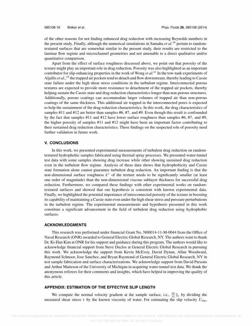
085108-16 Bidkar et al. Phys. Fluids 26, 085108 (2014)

of the other reasons for not finding enhanced drag reduction with increasing Reynolds numbers inthe present study. Finally, although the numerical simulations in Samaha et al.30 pertain to random-textured surfaces that are somewhat similar to the present study, their results are restricted to thelaminar flow regime and microchannel geometries and not amenable to a direct qualitative and/orquantitative comparison.

Apart from the effect of surface roughness discussed above, we point out that porosity of thetexture might play an important role in drag reduction. Porosity was also highlighted as an importantcontributor for slip-enhancing properties in the work of Wong et al.41 In the tow-tank experiments ofAljallis et al.,19 the trapped air pockets tend to detach and flow downstream, thereby leading to Cassiestate failure under the high shear stress conditions in the turbulent regime. Interconnected poroustextures are expected to provide more resistance to detachment of the trapped air pockets, therebyhelping sustain the Cassie state and drag reduction characteristics longer than non-porous structures.Additionally, porous coatings can accommodate larger volumes of trapped air than non-porouscoatings of the same thickness. This additional air trapped in the interconnected pores is expectedto help the sustainment of the drag reduction characteristics. In this work, the drag characteristics ofsamples #11 and #12 are better than samples #6, #7, and #9. Even though this result is confoundedby the fact that samples #11 and #12 have lower surface roughness than samples #6, #7, and #9,the higher porosity of samples #11 and #12 might have been an important factor contributing totheir sustained drag reduction characteristics. These findings on the suspected role of porosity needfurther validation in future work.

V. CONCLUSIONS

In this work, we presented experimental measurements of turbulent drag reduction on random-textured hydrophobic samples fabricated using thermal spray processes. We presented water-tunneltest data with some samples showing drag increase while other showing sustained drag reductioneven in the turbulent flow regime. Analysis of these data shows that hydrophobicity and Cassiestate formation alone cannot guarantee turbulent drag reduction. An important finding is that thenon-dimensional surface roughness k+ of the texture needs to be significantly smaller (at leastone order of magnitude) than the non-dimensional viscous sublayer thickness for successful dragreduction. Furthermore, we compared these findings with other experimental works on random-textured surfaces and showed that our hypothesis is consistent with known experimental data.Finally, we highlighted the potential importance of interconnected porosity of the texture in boostingits capability of maintaining a Cassie state even under the high shear stress and pressure perturbationsin the turbulent regime. The experimental measurements and hypothesis presented in this workconstitute a significant advancement in the field of turbulent drag reduction using hydrophobicsurfaces.

ACKNOWLEDGMENTS

This research was performed under financial Grant No. N00014-11-M-0044 from the Office ofNaval Research (ONR) awarded to General Electric Global Research, NY. The authors want to thankDr. Ki-Han Kim at ONR for his support and guidance during this program. The authors would like toacknowledge financial support from Steve Duclos at General Electric Global Research in pursuingthis work. We acknowledge the support from Kevin McEvoy, David Dynan, Allan Woodward,Raymond Schnoor, Jose Sanchez, and Bryan Raymond of General Electric Global Research, NY intest sample fabrication and surface characterizations. We acknowledge support from David Parsonsand Arthur Matteson of the University of Michigan in acquiring water-tunnel test data. We thank theanonymous referees for their comments and insights, which have helped in improving the quality ofthis article.

APPENDIX: ESTIMATION OF THE EFFECTIVE SLIP LENGTH

We compute the normal velocity gradient at the sample surface, i.e., ∂U∂y ‖s by dividing the

measured shear stress τ by the known viscosity of water. For estimating the slip velocity Uslip,

This article is copyrighted as indicated in the article. Reuse of AIP content is subject to the terms at: http://scitation.aip.org/termsconditions. Downloaded to IP:

141.212.194.165 On: Mon, 15 Jun 2015 10:50:21

085108-17 Bidkar et al. Phys. Fluids 26, 085108 (2014)

we adopt the approach of Fukagata et al.27 In particular, the slip velocity Uslip is estimatedusing

Uslip = Ub − Ube, (A1)

where Ub is the bulk mean velocity of the flow for the baseline (no-slip) case and Ube is the bulk meanvelocity of the flow for the hydrophobic sample (slip flow). We compute the bulk mean velocity Ub

for flow over a flat plate by integrating the flat plate velocity profile33 from y = 0 to the half-heighty = h of the water tunnel as follows:

Ub = 1

h

∫ δ

0

[1

κln

(yu∗

ν

)+ B + 2�

κ

(3( y

δ

)2− 2

( y

δ

)3)]

dy + 1

h

∫ h

δ

Udy, (A2)

where h = 0.1074 m is the half-height of the water tunnel, δ is the boundary layer thickness atx = 0.843 m, κ = 0.41, B = 5.0, and � = 0.45. Note that u* is based on test data for the baselineor the no-slip case and the boundary layer thickness δ is computed using the following equation:

U

u∗ = 1

κln

(δu∗

ν

)+ B + 2�

κ. (A3)

For the case of the hydrophobic sample (i.e., the slip flow case), we compute Ube using Eq. (A2)noting that u* is based on the test data from the hydrophobic sample. The boundary layer thicknessδ computed using Eq. (A3) is assumed to remain unchanged for both cases because the plate surfaceis identical for locations upstream of x = 0.843 m. Finally, the uncertainty bars shown in Figs. 9(a)and 9(b) are calculated using propagation of errors based on the uncertainty in the measured valuesof shear stress τ for the baseline sample #1 and the hydrophobic sample #12.

1 J. L. Lumley, “Drag reduction in turbulent flow by polymer additives,” J. Polym. Sci. Macromol. Rev. 7, 263–290 (1973).2 M. J. Walsh, “Riblets as a viscous drag reduction technique,” AIAA J. 21, 485–486 (1983).3 R. A. Antonia, Y. Zhu, and M. Sokolov, “Effect of concentrated wall suction on a turbulent boundary layer,” Phys. Fluids

7, 2465 (1995).4 W. C. Sanders, E. S. Winkel, D. R. Dowling, M. Perlin, and S. L. Ceccio, “Bubble friction drag reduction in a high Reynolds

number flat-plate turbulent boundary layer,” J. Fluid Mech. 552, 353–380 (2006).5 S. L. Ceccio, “Friction-drag reduction of external flows with bubble and gas injection,” Ann. Rev. Fluid Mech. 42, 183–203

(2010).6 K. Watanabe, Y. Udagawa, and H. Udagawa, “Drag reduction of newtonian fluid in a circular pipe with a highly water-

repellant wall,” J. Fluid Mech. 381, 225–238 (1999).7 J. Ou, B. Perot, and J. P. Rothstein, “Laminar drag reduction in microchannels using ultrahydrophobic surfaces,” Phys.

Fluids 16, 4635 (2004).8 A. K. Balasubramanian, A. C. Miller, and O. K. Rediniotis, “Microstructured hydrophobic skin for hydrodynamic drag

reduction,” AIAA J. 42, 411–414 (2004).9 S. Gogte, P. Vorobieff, R. Truesdell, A. Mammoli, F. Swol, P. Shah, and C. J. Brinker, “Effective slip on textured hydrophobic

surfaces,” Phys. Fluids 17, 051701 (2005).10 R. Truesdell, A. Mammoli, P. Vorobieff, F. Swol, and C. J. Brinker, “Drag reduction in a patterned superhydrophobic

surface,” Phys. Rev. Lett. 97, 044504 (2006).11 C. Henoch, T. N. Krupenkin, P. Kolodner, J. A. Taylor, M. S. Hodes, A. M. Lyons, C. Peguero, and K. Breuer, “Turbulent

drag reduction using superhydrophobic surfaces,” AIAA Paper 2006-3192, 2006.12 C. Choi and C. Kim, “Large slip of aqueous liquid flow over a nanoengineered superhydrophobic surface,” Phys. Rev. Lett.

96, 066001 (2006).13 J. Zhao, X. Du, and X. Shi, “Experimental research on friction reduction with superhydrophobic surfaces,” J. Mar. Sci.

Appl. 6, 58–61 (2007).14 C. Lee, C. Choi, and C. Kim, “Structured surfaces for a giant liquid slip,” Phys. Rev. Lett. 101, 064501 (2008).15 R. J. Daniello, N. E. Waterhouse, and J. P. Rothstein, “Drag reduction in turbulent flows over superhydrophobic surfaces,”

Phys. Fluids 21, 085103 (2009).16 B. Woolford, J. Prince, D. Maynes, and B. W. Webb, “Particle image velocimetry of turbulent channel flow with ribbed

patterned superhydrophobic walls,” Phys. Fluids 21, 085106 (2009).17 C. Peguero and K. Breuer, “On drag reduction in turbulent channel flow over superhydrophobic surfaces,” in Advances in

Turbulence XII, Springer Proceedings in Physics (Springer, 2009), Vol. 132, pp. 233–236.18 E. Aljallis, M. A. Sarshar, R. Datla, S. Hunter, J. Simpson, V. Sikka, A. Jones, and C. Choi, “Measurement of hydrodynamic

frictional drag on superhydrophobic flat plates in high reynolds number flows,” in Proceedings of ASME 2011 InternationalMechanical Engineering Conference and Exposition (IMECE2011-63272), Denver, CO, USA (ASME, 2011), pp. 77–82.

19 E. Aljallis, M. A. Sarshar, R. Datla, V. Sikka, A. Jones, and C. Choi, “Experimental study of skin friction drag reductionon superhydrophobic flat plates in high reynolds number boundary layer flows,” Phys. Fluids 25, 025103 (2013).

This article is copyrighted as indicated in the article. Reuse of AIP content is subject to the terms at: http://scitation.aip.org/termsconditions. Downloaded to IP:

141.212.194.165 On: Mon, 15 Jun 2015 10:50:21

085108-18 Bidkar et al. Phys. Fluids 26, 085108 (2014)

20 D. Bleecher, P. Harsh, M. Hurley, A. K. Jones, R. Ross, V. K. Sikka, and D. Zeike, “Highly durable superhydropho-bic, oleophobic and anti-icing coatings and methods and compositions for their preparations,” U.S. patent applicationUS2012/0045954 A1 (23 Feb 2012).

21 H. Park, G. Sun, and C. Kim, “Turbulent drag reduction on superhydrophobic surfaces confirmed by built-in shear sensing,”in Proceedings of 2013 IEEE 26th International Conference on MEMS, Taipei, Taiwan (IEEE, 2013), pp. 1183–1186.

22 H. Park, G. Sun, and C. Kim, “Superhydrophobic turbulent drag reduction as a function of surface grating parameters,” J.Fluid Mech. 747, 722–734 (2014).

23 N. A. Patankar, “On the modeling of hydrophobic contact angles on rough surfaces,” Langmuir 19, 1249–1253 (2003).24 J. P. Rothstein, “Slip on superhydrophobic surfaces,” Ann. Rev. Fluid Mech. 42, 89–109 (2010).25 E. Lauga and H. A. Stone, “Effective slip in pressure-driven stokes flow,” J. Fluid Mech. 489, 55–77 (2003).26 T. Min and J. Kim, “Effects of hydrophobic surface on skin-friction drag,” Phys. Fluids 16, L55 (2004).27 K. Fukagata, N. Kasagi, and P. Koumoutsakos, “A theoretical prediction of friction drag reduction in turbulent flow by

superhydrophobic surfaces,” Phys. Fluids 18, 051703 (2006).28 M. B. Martell, B. Perot, and J. P. Rothstein, “Direct numerical simulations of turbulent flows over superhydrophobic

surfaces,” J. Fluid Mech. 620, 31–41 (2009).29 K. Jeffs, D. Maynes, and B. W. Webb, “Prediction of turbulent channel flow with superhydrophobic walls consisting of

micro-ribs and cavities oriented parallel to the flow direction,” Int. J. Heat Mass Transfer 53, 786–796 (2010).30 M. A. Samaha, H. V. Tapreshi, and M. Gad el hak, “Modeling drag reduction and meniscus stability of superhydrophobic

surfaces comprised of random roughness,” Phys. Fluids 23, 012001 (2011).31 H. Park, H. Park, and J. Kim, “A numerical study of the effects of superhydrophobic surface on skin-friction drag in

turbulent channel flow,” Phys. Fluids 25, 110815 (2013).32 Teflon R© is a registered trademark of DuPontTM Co.33 F. M. White, Viscous Fluid Flow, 2nd ed. (McGraw Hill Inc., New York, 1991).34 L. F. Moody, “Friction factors for pipe flow,” Trans. ASME 66, 671–684 (1944).35 F. H. Clauser, “The turbulent boundary layer,” Adv. Appl. Mech. 4, 1–51 (1956).36 J. Nikuradse, “Strmungsgesetze in rauhen rohren,” Forsh. Arb. Ing.-Wes. 361, 22 (1933) [Laws of Flow in Rough Pipes,

NACA TM 1292, 1950].37 Skewness is defined as 1/(R3

q )(1/E)∫ E

0 (Z (x) − η)3dx . Rq is the rms roughness given by√

1/E∫ E

0 (Z (x) − η)2dx .38 C. Ybert, C. Barentin, C. Cottin-Bizonne, P. Joseph, and L. Bocquet, “Achieving large slip with superhydrophobic surfaces:

Scaling laws for generic geometries,” Phys. Fluids 19, 123601 (2007).39 J. Kim, P. Moin, and R. Moser, “Turbulence statistics in fully developed channel flow at low reynolds number,” J. Fluid

Mech. 177, 133–166 (1987).40 P. Orlandi and J. Jiminez, “On the generation of turbulent wall friction,” Phys. Fluids 6, 634–641 (1994).41 T. Wong, S. Kang, S. Tang, A. Grinthal, E. Smythe, B. Hatton, and J. Aizenberg, “Bioinspired self-repairing slippery

surfaces with pressure-stable omniphobicity,” Nature (London) 477, 443–447 (2011).

This article is copyrighted as indicated in the article. Reuse of AIP content is subject to the terms at: http://scitation.aip.org/termsconditions. Downloaded to IP:

141.212.194.165 On: Mon, 15 Jun 2015 10:50:21