Louisiana State UniversityLSU Digital Commons

LSU Historical Dissertations and Theses Graduate School

1994

Studies on the Diffusive Transport of HydrophobicOrganic Chemicals in Bed Sediments.Gregory John ThomaLouisiana State University and Agricultural & Mechanical College

Follow this and additional works at: https://digitalcommons.lsu.edu/gradschool_disstheses

This Dissertation is brought to you for free and open access by the Graduate School at LSU Digital Commons. It has been accepted for inclusion inLSU Historical Dissertations and Theses by an authorized administrator of LSU Digital Commons. For more information, please contactgradetd@lsu.edu.

Recommended CitationThoma, Gregory John, "Studies on the Diffusive Transport of Hydrophobic Organic Chemicals in Bed Sediments." (1994). LSUHistorical Dissertations and Theses. 5762.https://digitalcommons.lsu.edu/gradschool_disstheses/5762

INFORMATION TO USERS

This manuscript has been reproduced from the microfilm master. UMI films the text directly from the original or copy submitted. Thus, some thesis and dissertation copies are in typewriter face, while others may be from any type of computer printer.

The quality of this reproduction is dependent upon the quality of the copy submitted. Broken or indistinct print, colored or poor quality illustrations and photographs, print bleedthrough, substandard margins, and improper alignment can adversely affect reproduction.

In the unlikely event that the author did not send UMI a complete manuscript and there are missing pages, these will be noted. Also, if unauthorized copyright material had to be removed, a note will indicate the deletion.

Oversize materials (e.g., maps, drawings, charts) are reproduced by sectioning the original, beginning at the upper left-hand corner and continuing from left to right in equal sections with small overlaps. Each original is also photographed in one exposure and is included in reduced form at the back of the book.

Photographs included in the original manuscript have been reproduced xerographically in this copy. Higher quality 6" x 9" black and white photographic prints are available for any photographs or illustrations appearing in this copy for an additional charge. Contact UMI directly to order.

University Microfilms International A Bell & Howell Information Company

300 North Zeeb Road, Ann Arbor, Ml 48106-1346 USA 313/761-4700 800/521-0600

Order N um ber 9502149

Studies on the diffusive transport o f hydrophobic organic chem icals in bed sedim ents

Thom a, Gregory John, Ph.D.

The Louisiana State University and Agricultural and Mechanical Col., 1994

U M I300 N. ZeebRd.Ann Arbor, MI 48106

STUDIES ON THE DIFFUSIVE TRANSPORTOF

HYDROPHOBIC ORGANIC CHEMICALS IN BED SEDIMENTS

A Dissertation Submitted to the Graduate Faculty of the

Louisiana State University and Agricultural and Mechanical College

in partial fulfillment of the requirements for the degree of

Doctor of Philosophy

in

The Department of Chemical Engineering

byGregory John Thoma

B.S., University of Arkansas, 1980 M.S. University of Arkansas, 1986

May, 1994

Dedication

This work is dedicated to my wife, Eileen, whose love and encouragement make

it all worthwhile.

Acknowledgements

I would like to thank Drs. Thibodeaux, Reible, and Valsaraj for their guidance

during my research. I am also grateful for the many opportunities provided to me

which will prove invaluable in my career development. My research would not have

been possible without the help of many student workers and the interaction with the

other graduate students in the environmental chemical engineering group. Two student

workers, Chris Porter, who performed many of the colloid flux experiments, and Sachit

Verma, who performed the extractions required to generate the contaminant

concentration profiles both deserve special recognition because of their demonstrated

self-starting ability.

I would like to thank Dennis Timberlake of the EPA Risk Reduction Engineering

Laboratory in Cincinnati for support of my work on capping through grant number

CR820531-01-0. This capping project also received support from the EPA Hazardous

Waste and Hazardous Substance Research Centers at Louisiana State University.

Finally I wish to thank the Louisiana State Board of Regents for supporting me through

the Fellowship program. Without their financial support I would have been unable to

return to school.

Table of ContentsDedication ............................................................................................................................. ii

A cknow ledgem ents..............................................................................................................iii

A bstract ............................................................................................................................... ix

C hapter 1In tro d u c tio n ........................................................................................................................ 1

C hapter 2L iterature Review ............................................................................................................ 8

§2.1 Fate and transport mechanisms in bed sedim ents....................................... 9§2.1.1 Molecular d iffu sio n ......................................................................... 11§2.1.2 A dvection.......................................................................................... 12§2.1.3 Sorption processes............................................................................ 12§2.1.4 Biodegradation................................................................................. 14§2.1.5 Sediment transport ......................................................................... 15§2.1.6 Bioturbation .................................................................................... 16

§2.2 Colloidally facilitated contaminant transport ............................................ 17§2.2.1 Hydrophobic organic chemical partitioning to DOC ................ 19§2.2.2 Mobility/transport of co llo id s ....................................................... 21

§2.3 Capping contaminated sed im en ts ................................................................ 25§2.3.1 Gather project data ......................................................................... 28§2.3.2 Contaminated sediment characterization...................................... 28§2.3.3 Site selection considerations.......................................................... 30

§2.3.3.1 Long term integrity........................................................... 31§2.3.4 Selection and characterization of capping sed im en t.................. 32§2.3.5 Placement technique ...................................................................... 39

§2.3.5.1 Considerations fo r contaminated material placement. 39§2.3.5.2 Considerations fo r cap material placement.................. 40§2.3.5.3 Modified surface release.................................................. 41§2.3.5.4 Submerged discharge........................................................ 42§2.3.5.5 Geotextiles.......................................................................... 43§2.3.5.6 Navigation and positioning.............................................. 43

§2.3.6 Evaluate spread, mounding, consolidation, and erodability . . 44§2.3.7 Determining the required cap th ickness...................................... 45§2.3.8 Developing a monitoring p ro g ra m ............................................... 48

§2.3.8.1 Physical monitoring.......................................................... 48

iv

§2.3.8.2 Chemical monitoring......................................................... 49§2.3.8.3 Biological monitoring....................................................... 49

§2.4 Summary ........................................................................................................ 50

C hapter 3M aterials and M e th o d s ................................................................................................ 52

§3.1 Studies of contaminant release ................................................................. 52§3.1.1 Sedim ents.......................................................................................... 54

§3.1.1.1 Sediment preparation........................................................ 54§3.1.1.2 Characterization................................................................. 55

§3.1.2 Tracer s e le c tio n .............................................................................. 56§3.1.3 Partition coefficients ..................................................................... 57§3.1.4 Sediment in o cu la tio n ..................................................................... 58§3.1.5 Experimental apparatus.................................................................. 59§3.1.6 Simulator loading and operation ................................................. 60§3.1.7 Experimental design ..................................................................... 63

§3.2 Colloid transport s tu d ie s ............................................................................. 67§3.2.1 Sediments u s e d ................................................................................. 67§3.2.2 DOC partitioning ........................................................................... 68§3.2.3 Experimental apparatus.................................................................. 68§3.2.4 Experimental ap p ro ach .................................................................. 69

§3.2.4.1 DOC sediment profiles..................................................... 69§3.2.4.2 DOC flux to overlying water........................................... 71

§3.3 Colloid-facilitated contaminant transport ................................................. 72§3.3.1 Sediment p rep ara tio n ...................................................................... 72§3.3.2 Experimental apparatus.................................................................. 73§3.3.3 Simulator loading and operation ................................................. 73§3.3.4 Sediment in o cu la tio n ..................................................................... 73§3.3.5 Experimental design ..................................................................... 75

§3.4 Summary ......................................................................................................... 75

C hapter 4M athem atical M o d e lin g ................................................................................................ 77

§4.1 Modeling contaminant re le a se ..................................................................... 77§4.1.1 Development of a conceptual m o d e l........................................... 78

§4.1.1.1 Sediment-side and water-side resistances to masstransfer............................................................................. 79

v

§4.1.2 Development of mathematical m o d e ls ......................................... 83§4.1.3 Base c a s e ........................................................................................... 84§4.1.4 One-layer m o d e l............................................................................... 87§4.1.5 Two-layer model ............................................................................. 88 „§4.1.6 Sensitivity analysis .................................................................... 90

§4.2 Modeling DOC re le a s e ................................................................................. 94

§4.3 Modeling DOC facilitated transport .......................................................... 97§4.3.1 Sensitivity analysis ...................................................................... 102

§4.4 Summary ............................................................................................................105

C hapter 5Experim ental Results ......................................................................................................107

§5.1 Parameter measurement ................................................................................. 107§5.1.1 DOC partitioning ..............................................................................108§5.1.2 PAH partitioning ............................................................................... 109

§5.2 Mobility of natural D O C ..................................................................................113§5.2.1 DOC f l u x ............................................................................................ 113§5.2.2 DOC sediment p ro f ile s ....................................................................... 115

§5.2.2.1 Beaker profiles...................................................................... 115§5.2.2.2 Flow through cell profile.....................................................119

§5.3 Colloid facilitated transport ........................................................................... 121

§5.4 Capping experiments .......................................................................................121§5.4.1 Uncapped system s...............................................................................121

§5.4.1.1 Contaminant flux ................................................................126§5.4.1.2 Sediment concentration profiles......................................... 131

§5.4.2 Capped systems ..................................................................................137§5.4.2.1 Contaminant flux ...................................................................137§5.4.2.2 Sediment concentration profiles......................................... 148§5.4.2.3 Capped profiles..................................................................... 149

C hapter 6Model E v a lu a tio n ...............................................................................................................159

§6.1 Base case ...........................................................................................................160§6.1.1 Contaminant flux ...............................................................................160§6.1.2 Sediment profiles ...............................................................................162

vi

§6.2 One-layer m o d e l ................................................................................................ 164§6.2.1 Contaminant flux ..............................................................................164§6.2.2 Sediment profiles ..............................................................................166

§6.3 Two-layer m o d e l............................................................................................... 166§6.3.1 Contaminant flux ..............................................................................166§6.3.2 Sediment profiles ..............................................................................170

§6.4 DOC m o d e l........................................................................................................ 170§6.4.1 Flow through cells ............................................................................170§6.4.2 Beaker p ro file s ....................................................................................171

§6.5 DOC enhanced transport m o d e l...................................................................... 172

§6.6 Summary ............................................................................................................175

C hapter 7Conclusions and Recommendations ............................................................................177

§7.1 Conclusions........................................................................................................ 177§7.1.1 DOC mobility .....................................................................................177§7.1.2 Colloid facilitated tra n s p o r t ............................................................. 178§7.1.3 C ap p in g ................................................................................................ 178

§7.2 Recom m endations............................................................................................. 180§7.2.1 Colloid enhanced transport - experim en ta l.................... 180§7.2.2 Colloid enhanced transport - modeling .......................... 181§7.2.3 Capping - experim ental...................................................................... 181§7.2.4 Capping - m odeling ............................................................................183

B ib lio g rap h y ....................................................................................................................... 185

Appendix AQuality Assurance Objectives .................................................................................... 207

§A. 1 Data quality assessment ................................................................................. 207§A.1.1 P re c is io n .............................................................................................207§A.1.2 A ccu racy .............................................................................................210

§A. 1.2.1 Aqueous samples................................................................. 210§ A . 1.2.2 Solid samples....................................................................... 215

§A.1.3 Method detection l im it ......................................................................215§A.1.4 Representativeness ........................................................................... 216

vii

§A.2 Sampling p ro ced u res .......................................................................................216§A.2.1 Sample co llection ............................................................................. 216§A.2.2 Sample storage ................................................................................216

§A.3 Analytical procedures and calib ration .......................................................... 217§A.3.1 Analytical procedures .................................................................... 217

§ A . 3.1.1 Aqueous samples................................................................. 217§ A . 3.1.2 Solid samples....................................................................... 218§ A . 3.1.3 Determination o f partition constants................................. 218

§A.4 Calibration procedures and frequency.......................................................... 219§A.4.1 PAH analysis ...................................................................................219

§A.4.1.1 Dissolved organic carbon.................................................. 222

§A.5 Data reduction,validation, and re p o r tin g .................................................... 222§A.5.1 Data reduction .................................................................... 223

§A.5.1.1 Tracer flux ............................................................................223§ A. 5.1.2 Solids loading...................................................................... 224

§A.6 Internal quality control c h e c k s ......................................................................224§A.6.1 Aqueous s a m p le s .............................................................................. 224

§A. 6.1.1 PAH analyses.......................................................................224§A.6.1.2 Solid samples....................................................................... 226

§A.7 References to Appendix A ........................................................................... 226

Appendix BM ethod Detection Limit for Aqueous Samples ....................................................... 228

Appendix CColumn Extraction Procedure for Sediment S a m p le s ............................................232

Appendix DDerivation of the Solution to the Two Layer C a s e ..................................................235

Appendix ECom puter C o d e .................................................................................................................245

Appendix FSim ulator Cell D im ensions.............................................................................................261

Vita ..................................................................................................................................... 262

viii

Abstract

Hydrophobic chemicals have accumulated in sediments for most of the last century

as the result of industrial and municipal discharges as well as urban and agricultural

runoff to surface waters. Beginning with the Clean Water Act, these pollutant sources

have been significantly reduced resulting in the sediments becoming a source of

pollutants to the overlying water ecosystem. It is therefore important to determine the

rate at which the contaminants associated with the sediment are released to the water.

Removal or isolation of sediment-associated contaminants is often desirable. One

option for isolation of contaminated sediments from the aquatic ecosystem is capping,

the placement of clean (uncontaminated) sediment on top of the contaminated sediment.

After cap placement, molecular and Brownian colloidal diffusion will be the

dominant release mechanisms for sediment associated contaminants. Adsorbed

contaminant molecules will “piggy-back” diffusing colloids. Experimental results

demonstrating the mobility of natural colloids in diffusion controlled environments were

used to determine effective colloid diffusivities via a mathematical model. In addition,

preliminary verification of a simple mathematical model for colloid enhanced

contaminant release rate is presented. 22 mg/L of natural dissolved organic carbon

increased the flux of phenanthrene and pyrene by approximately 20% and 45%

respectively while the model predicted 10% and 35% enhancement.

Experimental and mathematical model results demonstrating the efficacy of capping

at isolating contaminated sediments are presented and discussed. Three to thirteen

millimeter caps of different sediments were used and an approximately 10 fold decrease

in the release rate through the cap compared to the release from uncapped sediments

after 50 days. Cap effectiveness was shown to be greatest immediately after placement

and to decrease with time.

The mathematical model predictions of the release dynamics compared favorably

with the observed experimental results. The modeling of capped systems provides the

basis for sound engineering design of caps as chemical containment barriers. The cap

properties found to be most significant in the chemical barrier property of a cap were

the thickness and organic carbon content. Both these properties tend to increase the

breakthrough time and to decrease the magnitude of the chemical release rate through

the cap.

x

Chapter 1 Introduction

The work presented in this dissertation was performed in the context of the

significant environmental problems which we currently face. In general the solution to

these problems requires first an understanding of the basic processes affecting the fate

of pollutants in the environment and second an application of this knowledge base to

the development of suitable remediation options. My work has addressed both of these

facets for the problem of contaminated sediments. The importance of contaminated

sediments is underscored by the estimated one-eighth to one-quarter of Superfund

National Priority List sites which include contaminated sediments (Wall, 1991).

Contaminated sediments exist because of past discharges to surface waters. These

discharges included industrial and municipal point sources as well as agricultural and

urban non-point source runoff. Often these discharges contained levels of hazardous or

toxic substances no longer regarded acceptable. Common contaminants included

nutrients, organic compounds (such as polynuclear aromatics, polychlorinated

biphenyls, and pesticides), and heavy metals. Many of these compounds are

hydrophobic, that is their aqueous solubility is low, and tend to partition to the organic

fraction of the suspended particulate and colloidal matter in streams and rivers. This

contaminated particulate load is deposited on lake and estuary bottoms becoming

incorporated into the bed sediments. Thus sediments have served as sinks for these

pollutants.

1

2

The sediment’s role is transformed from sink to source, and the pollutants will

move into the water column again, after elimination of the original source of pollution

because the water column will be rapidly flushed clean reversing the pollutant’s

chemical-potential gradient. Once the pollutant has returned to the water it may

volatilize (Southworth, 1979; Sodergren and Larsson, 1982; Thibodeaux and

Bosworth, 1990). Thus contaminated sediments may also pose an air pollution threat.

Because of the large, reversible sorptive capacity of most sediments for hydrophobic

compounds, unremediated contaminated sediments may unnecessarily increase the

incidence of disease in nearby human and wildlife communities for decades or possibly

centuries.

Some small level of contamination should be regarded as acceptable because natural

processes exist which will degrade most organic materials. It is the degradability of a

material which defines its acceptable level (concentration) in the environment.

Unfortunately, the degradability of most anthropogenic compounds is either not well

known or influenced by too many variables to be accurately predicted. Thus we must

operationally define what is acceptable. A public policy-based definition of acceptable

contamination rests on an assessment of the risk of increased disease in the local human

population attributable to exposure to a toxicant, not on nature’s capacity to detoxify

(Thibodeaux, 1990). Risk assessment relies on the identification and quantification of

two elements. First, the level of exposure of a receptor (human or animal) must be

evaluated. In the case of contaminated sediments this would include predicting or

measuring the release rate of the contaminant of concern into the water column, then

identifying all of the subsequent pathways by which the contaminant could be

transported to the receptor and estimating the cumulative exposure of the receptor. The

second element of risk assessment is associated with the toxicology of the particular

contaminant of concern, specifically, the dose-response characteristics for the receptor

must be evaluated. Knowing the exposure level and the dose-response characteristics

allows estimation of the risk. Site specific risk assessments grounded on accurate

chemical release rates serve as a primary tool for evaluating the need for and

effectiveness of remediation options. This evaluation is particularly important in light

of the great number of contaminated sites in the U.S. and the limited resource money

available for clean-up. One aspect of the work presented in this dissertation is focused

on and relevant to the first element of risk assessment: defining the release rate of

contaminants from sediments.

The first stage in assessing the contaminant release rate from sediments is to identify

the pertinent transport processes. Due to the tendency of many environmental pollutants

to sorb to the sediment phase, transport mechanisms between the sediment bed and

water column are generally the most important. The primary transport phenomena

operative within bed sediments are: adsorption-retarded diffusion, colloid-facilitated

diffusion, interstitial advection, erosion or deposition, and bioturbation (benthic

organisms circulating sediment particles and pore water). Each of these processes is

discussed in more detail in §2 .1.

Mathematical models developed with an understanding of these fundamental

environmental transport processes and used to asses a specific site will allow the most

4

cost-effective remediation. Information regarding the temporal and spatial distributions

of chemicals in the environment from these models is used to evaluate risks posed by

contaminated sites and to assess clean-up alternatives. As an example, four basic

options for remediation of contaminated sediments exist:

1) no-action (for example the contaminants are being naturally buried and areescaping to the water with insignificant effect),

2) dredging followed by upland treatment or disposal,

3) dredging followed by open water dumping and subsequent capping with cleansediment,

4) in-situ capping (when channel navigation requirements do not require removalof the contaminated sediment)

My major research effort focused on capping. Capping exploits the adsorptive

property of sediments to isolate contaminated sediments by placing a clean

(uncontaminated) sediment layer over the contaminated sediment. This should

effectively isolate the contaminants from the aquatic and benthic ecosystems, and thus

significantly reduce the associated risk. The isolation of the contaminated sediments by

a cap is effected through 1) elimination of bioturbation of pollutant laden particles, 2)

increasing the path length for diffusive and advective processes, and 3) eliminating

scour or resuspension of contaminated sediment. However, the effectiveness of this

technology has not been fully demonstrated. A primary objective my research was to

extend the scientific and engineering knowledge of the processes controlling the release

of hydrophobic pollutants from bed sediments and to quantify the degree to which

contaminated sediment may be isolated by a clean cap.

5

To further the understanding of capped contaminated sediment systems,

experiments using flow through cells containing both capped and uncapped

contaminated sediment were performed (§3.1). The effluent from the cells was

monitored for the analytes of concern (in these experiments polyaromatic hydrocarbons)

and the flux of the analyte was inferred from the effluent concentration and flowrate.

These results were compared to a mathematical model of the system (Thoma et

al. 1993a, Chapter 6). The mathematical model used to describe the contaminant

dynamics in the uncapped systems demonstrated good qualitative and quantitative

agreement with the experimental data. The model for contaminant dynamics in a capped

system exhibited the qualitative features observed in the laboratory data, but tended to

over predict the release rate by a factor of 2 to 4. These experiments are described

and discussed in Chapters 3 and 5, and the modeling is covered in Chapters 4 and 6.

After capping contaminated sediment, molecular and Brownian colloidal

diffusive processes will often be the dominant mechanisms driving the release of

contaminants from the sediment to the pelagic ecosystem. Contaminant molecules

adsorbed to colloidal particles will be “piggy-backed” with the colloid, and if the

colloid-contaminant complex crosses the sediment water interface, the contaminant flux

will be enhanced. In their review, McCarthy and Zachara (1989), point out several

studies in which aquifer colloids are thought to have been responsible for significantly

extending the range of contamination. The presence of colloidal particles in sediment

interstitial waters has been long known (Thurman, 1985; Brownawell 1986); however,

the potential for colloid enhanced transport of chemical contaminants has not been well

studied in sediment systems. Another phase of my research focused on the Brownian

diffusive transport of naturally occurring colloids and associated hydrophobic organic

contaminants. They were undertaken with the aim of defining the importance of this

contaminant transport mechanism in sediment beds and consisted of two stages outlined

below.

Prior to considering the effect of colloids on contaminant transport, a series of

experiments was conducted using flow through cells containing sediment to clarify the

transport behavior of the colloids themselves (§3.2.3). The effluent from these cells was

monitored for dissolved organic carbon (DOC) concentration (used as a surrogate

measure of the quantity of colloids) which, together with the measured flowrate, was

used to infer the release rate of colloids from the sediment. This work showed that,

in the laboratory systems used, colloids behave similarly to hydrophobic organic

compounds (HOCs) exhibiting a rapidly decreasing flux (release rate) to the overlying

water. The flux versus time profile was used to estimate an in-bed diffusivity for the

colloids through comparison of the data to a mathematical model of the process

(Valsaraj et al. 1993a). Experiments to demonstrate the effect of natural colloids on

the transport of HOC were performed using washed (colloid free) sediment in parallel

with sediment which had been frozen to increase the fraction of mobile colloids in the

sediment. Differences in the observed contaminant release rate for the two sediment

treatments was explained using a simple model for the enhancement effect of colloids.

These experiments are described and discussed in Chapters 3 and 5, and the modeling

is covered in Chapters 4 and 6.

7

This work provides a firm theoretical basis (through mathematical modeling) and

experimental verification of chemical release from sediments and the design of

contaminant containment through the use of clean cap material.

The structure of this dissertation is based on the division of the two focal areas

which are capping as a remediation alternative for contaminated sediments and colloidal

transport of contaminants. Chapter 2 presents a review of the available literature,

covering first the basic transport phenomena important in sediments and then reviewing

the overall capping procedure from an engineering perspective.

Chapter 2 Literature Review

Contaminated sediments exist as non-point pollutant sources in the natural

environment. Very little information exists which is useful in characterizing the effect

of contaminated sediments as pollutant sources. A clear understanding of the underlying

transport mechanisms responsible for pollutant movement in contaminated sediments is

necessary for this characterization as well as before rational cap design as a chemical

barrier is possible. Fate processes, specifically chemically- and biologically-mediated

degradation, must also be considered due to the long-term containment potential

afforded by a cap. The first section of the following review concentrates on the basic

transport and fate processes active in bed sediments. Special emphasis is given to the

effect of naturally occurring colloids on the transport of chemical contaminants because

of the potential importance of this mechanism in diffusion dominated systems likely to

develop after cap placement.

Action to mitigate the opportunity for human or wildlife exposure to pollutants

is usually desirable. One proposal to isolate contaminated sediments is covering them

with uncontaminated sediments. This appears to be simple proposition. However, as

the following review of the available literature will show, there are many considerations

which make this simple concept a challenge to design and execute. Twenty-one field

scale demonstrations are identified, yet most have focused on cap placement techniques

and stability. Although some chemical migration monitoring has been performed, the

monitoring design was not aimed at allowing the development of design tools, generally

using 1 cm or greater sections in cap cores without flux measurements. The laboratory

scale investigations on capping effectiveness have used (non-sorbing) nutrients as the

model compounds leaving open the question of the importance of the cap’s sorptive

capacity in mitigating chemical release.

The structure of the review of capping is directed by the engineering aspects of

designing capped contaminated sediment projects. The two primary requirements for

a successful capping operation are isolation of the ecosystem from the contaminants of

concern and maintaining the long-term integrity of the chemical seal. A review of

armoring techniques, which maintain the physical integrity of submerged structures

(e.g. caps), is available (Thoma, Reible and Timberlake, 1993b).

Recent reviews of the contaminant transport in sediments are available (Singh,

Reible and Thibodeaux, 1988; Medine and McCutcheon, 1989; Reible, Valsaraj and

Thibodeaux, 1991). The effects of colloids on the chemistry and transport of

contaminants in aquatic systems and the subsurface have been published (O’Melia,

1989; Pelizzetti and Maurino, 1990; Sigleo and Means, 1990; McCarthy and

Zachara. 1989). A review by Puls (1990) focuses on inorganic colloids and

radionuclide transport in the subsurface.

§2.1 Fate and transport mechanisms in bed sediments

Various mechanisms are responsible for the fate and transport of chemicals in

sediments. For hydrophobic chemicals these include:

10

★ Pore level processes

• Molecular and Brownian diffusion in the sediment interstitial water. These two processes are the topics of the remaining chapters.

• Advection due to hydraulic gradients in the sediment.

• Adsorption/desorption between the sediment particles and the adjacent pore-water.

• Chemical reaction and biodegradation.

★ Particle movement processes

® Sediment particle transport includes deposition, resuspension and bedload movement (shifting of the surficial sediment layer without resuspension).

• Bioturbation induced transport is a catch-all term for the effect of bottom dwelling (benthic) organisms.

Figure 2.1 is a schematic of the physico-chemical processes affecting

contaminant fate and transport from sediments to the overlying water column. Not all

of these mechanisms will be effective at each site. The most important modes in

uncapped sediments are likely to be bioturbation and resuspension since these processes

are responsible for the movement of contaminated sediment particles and are not

attenuated by sorptive processes within the sediment. While the most important after

cap placement are likely to be diffusion, colloid-enhanced diffusion, and advection. To

provide a background understanding of these processes in sediments, each is briefly

discussed below. A separate heading is devoted to the review of colloid-facilitated

transport since it is one of the two primary topics of theoretical and experimental

investigation discussed in the following chapters.

11

Air

Evaporatio]HDeposition

Water

"Mobile Bed" Type Bottom Form

0mmSuspended Sedimem A

© H ®Ripple or Dune

"Mud Flats" Type Bottom Form

Bedrock

1. Benthic Boundary Layer2. Diffusion

Molecular & Brownian (Colloids)3. Bioturbation4. Groundwater Exchange5. Localized Advection6. Particle Resuspension7. Particle Depositon8. Bed Translocation9. Biotransformadon / Degradation10. Gas Bubble Advection11. Fecal Mound

Worms

Bed Sediment

IIGround Water

Figure 2.1 Schematic of the fate and transport mechanisms in bed sediments.

§2.1.1 Molecular diffusion. Formica et al. (1988) report on the diffusion of

PCBs into bed sediments from a contaminated water layer and found that sorption to

the sediment phase significantly affected the observed sediment profiles. Di Toro, Jeris

and Ciacia (1985) performed careful studies on the partitioning and diffusion of

hexachlorobiphenyl in sediments reporting observed profiles which were described by

a sorption-diffusion model. Baron et al., (1990) studied the release of model

contaminants from (oil) drilling mud which is often disposed on the ocean floor. Often

contaminant profiles in the field exhibit a diffusion-like character (Eisenreich et a l.,

1989), showing depletion at the surface (indicative of contaminant transport out of the

12

sediment) and a long tail of decreasing concentration in the deeper sediment. Boudreau

(1986) points out that non-local mixing phenomena can also result in similar profiles,

so that the existence of these profiles does not necessarily indicate that molecular

diffusion is the cause of the profiles.

§2.1.2 Advection. Normal groundwater interactions may result in the bulk flow

of water through the interstices of a sediment bed. In addition, cyclic processes such

as tides, and local hydraulic gradients can induce pore-water flow. Thibodeaux and

Boyle (1987) has reported experimental and model results in which wake separation on

the downstream side of natural bed forms (dunes) in riverine systems caused local low

pressure which induced flow through the dune. This flow would of course impact the

transport of contaminants in those sediments, van Genuchten and Alves (1982) have

compiled many solutions to the solute advection-diffusion-reaction equation subject to

various boundary conditions.

§2.1.3 Sorption processes. The dynamic redistribution of contaminants implied by

adsorption/desorption partitioning has a significant effect on the rate of contaminant

movement through sediment beds. It is also one of the phenomena which capping relies

upon for its effectiveness. The rate of chemical transport due to both pore-water

advection and molecular diffusion is retarded by sorption between the pore-w ater and

the (stationary) sediment particles. The degree of retardation of these pore level

processes is primarily a function of the degree of hydrophobicity of the chemical in

question. A chemical’s hydrophobicity is quantified by its octanol-water partition

coefficient, Kow, which is the ratio of the octanol phase activity to the water phase

13

activity at equilibrium: Kow = y w Vwj (y0V0) where Vw and V0 are the water and

octanol molar volumes and y w and y 0 are the water and octanol activity coefficients of

the solute. Since the molar volumes are constants and the activity of many organic

solutes in octanol is small (1-10, Valsaraj et al., 1993b), Kow is a direct indicator of the

activity coefficient in water.

The partitioning behavior of an organic compound in an octanol-water system

is an excellent predictor of the chemical’s partitioning behavior between soils/sediments

and water in the environment. In soil and sediment systems the organic-carbon

normalized partition coefficient, Koc, is commonly used instead of the octanol-water

partition coefficient. The mechanism of partitioning in soils and sediments with greater

than 0.1% organic carbon is thought to be primarily through hydrophobic interaction

as it is in octanol water systems. This has led to the development of linear free energy

relationships between Koc and Kow of the form: log (Koc) = a ■ log(Kow) + b. Curtis

et al. (1986) report values for a and b of 0.92 and -0.23. Voice and Weber (1983) and

Curtis et al. (1986) have presented excellent reviews of sorption by sediments. Linear

free energy relationships are not recommended for compounds with polar functional

groups nor for sorbents with very low organic carbon contents. Because of the

importance of this quantity (Koc) and its relation to Kow, many compilations of the

values of Kow (since it is more easily measured) have been generated (Montgomery and

Welkom, 1990; Sunito et al, 1988; Mackay and Shiu, 1981; Sangster, 1989).

Lyman, Reehl and Rosenblatt (1990) present methods for estimating Knw based on group

contribution methods.

14

Hydrophobic chemicals will also partition to the organic fraction of natural

colloids present in sediment systems. This partitioning provides the basis for enhanced

contaminant transport mediated by the colloid fraction. This will be discussed in

greater detail in section §2.2.

§2.1.4 Biodegradation. A potentially significant benefit of a cap is to provide

containment of the contaminants while these fate processes degrade or detoxify them.

Many compounds once thought to be refractory are now known to degrade in the

natural environment. Reductive dechlorination of polychlorinated biphenyls (PCBs) has

been reported (Brown et al., 1984; Brown et al., 1987; Quensen, Tiedje and Boyd,

1988). Yutani (1983) reported that PCBs sorbed to sediment particles were degraded

more slowly than those in solution by comparing the degradation rate in carbon rich

sediment to that in charred (450°C 20 hr) sediment. Unterman et al. (1988) reported

on the mechanism of PCB dechlorination as mediated by microbes which involve a

dioxygenase attack on the PCB skeleton. Mills et al. (1991) have performed field

studies of the effect of white rot fungus on the biodegradation of PCB contaminated

soil. Soil concentrations were reduced from 340 and 220 ppm to 70 and 12 ppm on two

separate plots. Bauer and Capone (1988) and Mueller et al. (1991) reported on the

biodegradation of polyaromatic hydrocarbons (PAHs); however, Mueller et al. (1991)

observed little decrease in the teratogenicity or toxicity of the soil with degraded PAHs.

Sugiura (1992) showed that the degradation rate of PCBs in shaker flasks was enhanced

by the addition of an additional carbon substrate, while the apparent loss of

benzo(a)pyrene from soil amended with cow manure was unchanged compared to

unamended soil (Coover and Sims, 1987). Readman, Mantoura and Rhead (1987)

studied the PAH profiles in the Tamar estuary, U.K. and found primarily non-alkylated

parent forms indicative of pyrogenic sources. They conclude that little

biotransformation of the PAH occurs in these sediments. Although biodegradation has

received considerable attention, prediction of the degradation rates in the natural

environment are still uncertain. Clearly the design of a cap should incorporate

knowledge of the potential degradation of the contained compounds, and while this topic

is not considered in this dissertation, the need for continued study should be noted.

§2.1.5 Sediment transport. Flow induced resuspension and the subsequent

deposition of sediment particles as well as flow induced sliding or slipping of the

surficial sediment particles (bed load transport) is responsible for translocation of

contaminated areas as well as for exposing formerly buried contaminated sediment to

the water column. Lau, Oliver and Krishnappan (1989) studied contaminant transport

in the St. Clair and Detroit Rivers and found that the largest contaminant load was

associated with suspended sediment. This is in a locale which still receives large

industrial discharges, but it demonstrates that suspended sediment contaminant loads can

be important. Onishi (1981) has proposed a mathematical model which incorporates

contaminated sediment scour, deposition, and transport as well as contaminant-sediment

adsorption processes. Uncles, Stephens and Woodrow (1988) presented a contaminant-

sediment dynamics model for an idealized estuary. Savant-Malliet and Reible (1993)

reported experimental and model results showing the effect of bed load transport on

contaminant release from sediments. Bed load transport occurs when the water velocity

16

is not sufficient to resuspend sediment particles, but the drag force along the surface

is sufficient to cause rolling and sliding of surficial particles. This action was shown to

expose previously buried sediment to the sediment water interface thus allowing the

release of contaminants. Lane, Hakonson and Foster (1987) and Singh et al. (1988)

have reviewed sediment transport models in regard to contaminant transport in

watersheds and estuaries respectively.

§2.1.6 Bioturbation. Sediments harbor a great variety of life. The organisms

living in the sediment (benthos) are often very active processors of the sediment,

continually mixing the surface layers. This mixing of the sediment, known as

bioturbation, is the result of burrowing, tube building, ingestion and defecation of

sediment and other life activities of the benthos. Contaminants associated with sediment

particles are moved with the particles, and this may cause once buried contaminants to

be brought to the sediment water interface and be released to the overlying water. Root

systems and animal burrows may also provide preferential flow paths for water and

solute transport. Excellent reviews of the effect of bioturbation on contaminant transport

have been published (Aller, 1982; Lee and Schwartz, 1980).

Karickhoff and Morris (1985) estimated that pollutant flux from a freshwater

sediment was increased 4 to 6 times in the presence of worms. Renfro (1973) reported

3 to 7 fold increase in 65Zn flux from sediments in a flowing seawater microcosm

inhabited by a marine clam. Benthic infauna (animals living in the sediment) have been

shown to increase the rate of incorporation of 35S into the sediment (Lawrence and

Mitchell, 1985). Riedel, Sanders and Osman (1987) compared the flux of As from a

17

sediment bed under the influence of polychaete worms and complete episodic

resuspension and found that either of these treatments increased the flux approximately

5 times compared to controls. Cullen (1973) observed that the tracks of fiddler crabs

disappeared 12 days after the removal of the crabs from a system isolated from external

disturbances. This action was attributed to meiofauna, animals only a millimeter or less

in length, indicating that not only worms and larger animals can be effective

bioturbators. Aller and Aller (1992) have quantified the effect of meiofauna on solute

transport in marine muds.

§2.2 Colloidally facilitated contaminant transport

Situations will exist where the transport is dominated by molecular diffusion

retarded by sorption/desorption with the immobile sediment. Under these conditions

the presence of organic colloids in the pore water may enhance the flux of hydrophobic

organic compounds (HOCs) over that of simple retarded diffusion (Enfield, Bengtsson

and Lindqvist, 1989; McCarthy and Zachara, 1989). Dissolved organic compounds

originating from decaying plant and animal matter, are the primary source of colloidal

material in sediments. Colloidal particles, defined arbitrarily as particles with mean

diameters between 0.002/xm and 0.45/im (2 to 450 nanometers), are primarily

comprised of aggregates of humic and fulvic acids that are stable in low salinity

environments (Thurman, 1985). Frequently the easily measured quantity, dissolved

organic carbon (DOC) is used as a surrogate measure of the quantity of colloids

present (Brownawell and Farrington, 1986). In the remainder of this document the

18

acronym DOC will refer to this surrogate measure of the quantity of organic colloids

present. DOC concentrations from 10 to 390 mg/L for anaerobic interstitial sediment

waters have been reported (Thurman, 1985). In groundwater systems colloids also

arise from the precipitation of inorganic constituents present in the water, for example,

van der Lee, Ledoux and de Marsily (1992) discuss the transport of radionuclides

through fractured media under circumstances such that (in this case) colloidal uranium

particles are formed. This type of colloid is called an intrinsic or type I colloid. The

colloids generated from a source distinct from the compound of interest (i.e. the DOC

introduced above) are known as type II colloids. From this point forward, the term

colloid should be taken to mean type II colloids only.

Colloids have been postulated to explain the “sediment concentration effect” in

laboratory tests where the HOC sediment-water distribution coefficient has been

observed to depend on the sediment concentration in the reactor (Servos and Muir,

1989; Gschwend and Wu, 1985; Mackay and Powers, 1987). However, not all

investigators are in agreement(Di Toro et al., 1986). Similarly, in the air, colloids

have also been implicated in the enrichment of certain pesticides in fog water as

compared to what is predicted by Henry’s law partitioning (Glotfelty, Seiber and

Liljedahl, 1986; Glotfelty, Majewski and Seiber, 1990; Capel, Leuenberger and

Giger, 1991; Schomburg, Glotfelty and Seiber, 1991; Valsaraj et al., 1993b).

The mechanism of colloidal facilitation of contaminant transport in sediments is

depicted in Figure 2.2. Adsorbed HOCs will be carried piggy-back across the sediment

water interface by the Brownian movement of the colloidal particles in addition to

19

Air

Water

! Sediment.

• Pollutant Q Colloidal particle | - | Immobile sediment

Figure 2.2 Schematic of colloid facilitated contaminant transport

molecular diffusion of the solute out of the pore water. Of course, both binding of the

contaminant to the colloid and mobility of the colloid are necessary for facilitated

transport to occur. Each of these aspects will be discussed below.

§2.2.1 Hydrophobic organic chemical partitioning to DOC. A great deal of effort

has been put forth studying the partitioning of hydrophobic organic chemicals between

dissolved organic colloids and aqueous phases (e.g. Hassett and Anderson, 1979;

Means et al., 1980; Hassett and Anderson, 1982; Schellenberg, Leuenberger and

Schwarzenbach, 1984; Hassett and Millicic, 1985; Haas and Kaplan, 1985; Caron,

Suffet and Belton, 1985; Gschwend and Wu, 1985; Walters et al. , 1989; Servos and

20

Muir, 1989). Organic colloids have a large capacity to bind HOCs (Brownawell and

Farrington, 1986; Means and Wijayaratne, 1982; Hassett and Anderson, 1979).

Brownawell and Farrington (1985) measured PCB concentrations in the interstitial water

of sediments in New Bedford Harbor, MA and found that a significant fraction of the

interstitial PCBs were associated with colloidal particles. Chiou et al. (1986) reported

solubility enhancement for some pesticides and PCBs in the presence of dissolved humic

substances. Means et al. (1982) showed DOC-water partition coefficients 10 to 35 times

higher than sediment-water partition coefficients for two pesticides. Rav-Acha and

Rebhun (1992) report on experiments and modeling to describe the effect that colloids

have on the partition coefficient between water and solid phase. In some instances the

observed partition coefficient (measured without separating the colloids from the

aqueous phase) increases with the presence of colloids and sometimes it decreases.

They postulate that this is due to the partitioning of the colloid-contaminant complex.

When the complex (i.e. the colloid) to sediment partitioning is greater than the solute

to sediment partitioning, the apparent solute partition coefficient is increased. The

more common observation is that the colloids solubilize the solute (i.e. the complex is

less strongly bound than the free solute) thereby decreasing the observed solute partition

coefficient.

Koulermos (1989) reported anomalously high partition constants for naphthalene

to DOC which decreased as DOC concentration increased, leveling off at a value of

approximately 5 times the literature value for organic carbon normalized sediment-water

partition coefficient, Koc. Landrum et al. (1984) have shown a decreasing trend for

21

humic acid-water partition coefficients for several hydrophobic organic chemicals as a

function of humic acid concentration. However Herbert, Bertsch and Novak (1993)

found that the organic carbon normalized partition coefficient (Koc) of pyrene to natural

dissolved organic matter (DOM) was smaller by an order of magnitude than the value

of Koc reported for soils. They also report that the value of K()C varied depending on

the fraction of the DOM (size fractionated). Koc was larger for the more hydrophobic

DOM fraction. Murphy, Zachara and Smith (1990) observed similar behavior for clays

coated with various natural humic substances. Gauthier, Seitz and Grant (1987)

reported values of Koc for pyrene on a series of well characterized DOM from different

sources. The (log) values ranged from 4.5 to 5.5 (avg 4 .9+0.31) and increased with

increasing DOM aromaticity as indicated by I3C NMR and UV absorptivity at 272 nm.

Montgomery and Welkom (1990) report a value of logfK^) for pyrene of 4.8 + 0.2

for sorption to soils.

§2.2.2 M obility/transport of colloids. In addition to binding of pollutants, the

pollutant-colloid complex must be mobile in the porous medium before enhanced

transport will be observed. Many factors affect the mobility of colloidal particles in

aquatic systems. The two most significant are the electrical double layer (EDL) and

van der Waals (VDW) forces. The electric double layer arises in solution because ions

tend to accumulate near surfaces. The surface of a natural particle has a net charge and

to balance this local charge, counterions enshroud the particle. It is the combination

of ions on the surface and the surrounding counterions that is known as the electric

double layer. These two effects (EDL & VDW) act in opposition and together define

22

the stability of colloidal suspensions. Quantitative relationships between these forces

have been formalized in DLVO theory after Derjaguin, Landau, Vervey, and Overbeek.

The essence of the theory is to estimate the van der Waals attractive forces for some

geometry and then combine this with estimated electrical double layer repulsive forces.

Solution chemistry is an important determining factor in the development of the EDL.

Specifically, the ionic strength and valence of the counterions determine the thickness

of the EDL and thus the strength of the stabilizing repulsive force acting on the

colloids. As an example, in the case of sedimentation in estuaries, it is the increasing

ionic strength of the estuarine water (along the land-sea axis) which is partly responsible

for the deposition of river borne suspended sediment. The increasing ionic strength

causes the EDL to collapse and allows VDW forces to begin to dominate. This

ultimately causes coagulation of the particles which then settle due to gravity.

A tremendous body of literature regarding the behavior of colloidal particles

exists. O ’Melia (1989) has presented a recent review of the effects of particles in

natural systems. The topics covered include particles, pollutants, and colloidal stability;

particle pollutant reactions; humic substances and colloidal stability; and particle

passage and retention in groundwater aquifers. Most textbooks on interfacial

phenomena or the physical chemistry of surfaces provide a section on DLVO theory

(e.g. Adamson, 1990; Miller and Neogi, 1985). However, a recent paper (Ellmelech

and O ’Melia, 1990) studying the deposition of latex colloidal particles in a porous

medium (glass beads) showed that DLVO theory alone is not adequate to describe the

colloidal deposition. Thus DLVO theory is a good guide for determining what factors

23

should be considered, but is not yet complete enough to give accurate quantitative

results in complex systems.

Thoma et al. (1991) have presented a simple model of hydrophobic organic

chemical flux enhancement due to the presence of DOC in a diffusion controlled

regime. For highly hydrophobic compounds significant enhancement is predicted

compared to the case in which colloids are absent, but little or no effect is predicted for

compounds with log(Kow) less than approximately 3.5 to 4. Enfield and Bengtsson

(1988) present a model for colloidal enhancement of contaminants in a groundwater

flow regime and, for moderate levels of DOC in solution, similar enhancements to the

relative mobility of contaminants in the subsurface are predicted. Again, for log(K<,w)

less than 4, very little increase in contaminant mobility is expected.

Enfiled (1985) and Enfield et al. (1989) have investigated the mobility of

macromolecules in groundwater and shown that, under some conditions, they can move

faster than tritiated water through a soil column due to size exclusion of the

macromolecules from the smallest pores. Hydrophobic organic chemicals were shown

to sorb to the macromolecules and thus exhibited enhanced transport. Puls and Powell

(1992) studied the stability and transport of radiolabeled iron oxide particles in column

experiments. They studied the effect of ionic strength and electrolyte composition, pH,

flowrate, particle size and concentration. The highest correlation to the breakthrough

was with the particle size and the anionic composition of the electrolyte; size exclusion

was observed under some conditions. Habere and Brunner (1993) present a complex

model of the effect of colloidal particles on contaminant transport rate accompanying

24

groundwater flow through a porous medium using the generalized Taylor-Aris

dispersion scheme. These experiments and models are applicable in a flow regime.

Similar studies in a diffusion controlled regime were not found in the literature. It is

important to extend the understanding of this phenomenon to the diffusion controlled

regime for two reasons. Diffusive transport is ubiquitous and its effects should be

clearly understood in the analysis of natural systems. The second is the applied

extension of the first: contaminated sediment sites exist in which molecular diffusion

controls the release of contaminants to the ecosystem (Thibodeaux and Bosworth,

1990), and in order to assess the risk associated with these sites the source strength

must be known so that exposure estimates can be made.

Thoma et al. (1991) have presented the results of preliminary investigations into

the flux enhancement of hydrophobic organic chemicals by colloids. An (initially)

homogeneous sediment bed, prepared in a 1 L beaker, was cored and sectioned after

97 days (the overlying water was changed every 2 days), and the sections centrifuged

to obtain a pore water sample which was analyzed for DOC. A distinct DOC

concentration profile was observed, clearly indicating that the DOC diffused from the

sediment to the overlying water. A simple model of the diffusion process was used to

estimate a diffusivity for the DOC. A second experiment in which DOC were allowed

to accumulate in the overlying water yielded a second estimate of DOC diffusivity, and

the Stokes-Einstein relation applied to size fractionated DOC provided a third. The

estimated diffusivities varied over an order of magnitude for the same sediment

depending on the measurement technique. Physically the boundary conditions in these

25

experiments was poorly characterized and time varying. Thus extension of this work

was undertaken to provide a physical model which could be more appropriately

modeled with simple time-invariant boundary conditions.

In sediment interstitial waters, both the redox potential, E,,, and the pH change

with depth. Since most of the chemistry of the sediment can be described in terms of

acid-base and oxidation-reduction reactions, the Eh and pH largely determine the

chemical species which may be found at any particular location (Day et al., 1989).

Thus the ionic strength (and the stability of colloids) might be expected to vary with

depth in the sediment bed. In addition, the salinity gradient found along all estuaries

will influence the stability of colloids at various places in the estuary. Thus a

comprehensive model of colloidally enhanced pollutant flux should include these

considerations. Nevertheless, the work presented in §4.2 demonstrates that for the

systems studied, the behavior of DOC is very similar to that expected for a single,

sorbing chemical species.

§2.3 Capping contaminated sediments

Capping, as defined on p4, is the placement of uncontaminated sediment on top

of a layer of contaminated sediment. Capping is considered an appropriate contaminant

control measure for benthic effects in the Army Corps of Engineers’ dredging

regulations (33CFR 335-338) and is recognized by the London Dumping Convention

as a management technique to rapidly render harmless otherwise unsuitable materials

(Edgar and Engler, 1984). Typically contaminated sediments cover large areas and thus

26

the volume qf sediment (and water) which requires treatment is large. This fact poses

a significant problem in terms of traditional (dredge and treat) remediation options.

Additional concerns center on the disturbance of the relatively stable environment

during dredging.

There are four fundamental alternatives for remediation of contaminated

sediment sites:

1) no-action (for example the contaminants are being naturally buried and areescaping to the water with insignificant effect),

2) dredging followed by upland treatment or disposal,

3) dredging with open water dumping and subsequent capping with clean sediment,

4) in-situ capping (when channel navigation requirements do not require removalof the contaminated sediment).

In this document the term ’capping’ will be used generically to refer to either

of the last two options. Palermo (1991a) states

“Level Bottom Capping may be defined as the placement of a contaminated material on the bottom in a mounded configuration, and the subsequent covering of the mound with a clean sediment. Contained Aquatic Disposal is similar to LBC but with the additional provision of some form of lateral confinement (for example, placement in bottom depressions or behind subaqueous berms) to minimize spread of the materials on the bottom.”

Figure 2.3 shows schematics of LBC and CAD (Palermo, 1991b).

The significant advantages of capping include:

• eliminating direct bioturbation of the contaminated sediment layer, reducingboth bioavailability and contaminant release to the water column (§2.1.6),

• increasing the diffusive and advective transport lengths and providing additionalsorption capacity within the sediment (§2.1.2),

27

• LATERAL CONFINEMENT• MOUND L E S S CRITICAL

• NO LATERAL CONFINEMENT• DISCRETE MOUNO NECESSA RY

LATERAL CONFINEMENT

CONTAMINATED MATERIAL

CAPPING MATERIAL

CONTAINED AQUATIC DISPOSAL LEVEL BOTTOM CAPPING

Figure 2.3 A) Confined aquatic disposal B) Level bottom capping.

• eliminating resuspension and direct desorption of pollutants to the water column associated with dredging and ex-situ treatment (or storms, propeller wash, etc).

Capping is likely to be used only in environments where the long term physical

integrity of the cap can be guaranteed. Typically this would mean low hydrodynamic

energy environments such as estuary or lake bottoms; however, armoring techniques exist

which may make capping viable in other areas as well. It should be recognized however,

that even a cap which requires periodic maintenance to maintain the design thickness may

be more effective and economic than alternative treatment technologies.

A considerable body of literature exists on the subject of subaqueous capping.

Much of the work in this area is associated with the handling of contaminated dredged

material removed from navigation channels performed by or in cooperation with the US

Army Corps of Engineers. Bokuniewicz, Cerrato and Hirschberg (1986) present a

general discussion covering many aspects of capping including cap stability, benthic

28

general discussion covering many aspects of capping including cap stability, benthic

recolonization and contaminant containment. Averett et al. (1990) review remediation

technologies (in general) for contaminated sediments in the Great Lakes. Palermo

(1991a) has presented a concise guide applicable to all capping projects, and Shields

and Montgomery (1984) and Montgomery (1983) provide an overview of engineering

considerations for capping projects. I reproduce the design flowchart from Palermo

(1991a) as Figure 2.4, and will use the design sequence presented there as an outline

for the literature review.

§2.3.1 G ather project data. Existing data on a site should first be compiled and

evaluated for completeness and applicability to selection and design of a cap. Available

data might include information regarding the contaminated sediment (testing performed

under 404 of the CA or 103 of the Ocean Dumping Act to determine the suitability for

open water disposal), surveys of the area, and data on potential placement sites. Three

aspects of the capping project must ultimately be examined and assessed for

compatibility: characterization and placement of the contaminated sediment,

characterization and placement of the capping material, selection of placement

equipment and capping site.

§2.3.2 Contam inated sediment characterization. Physical, chemical, and

biological characterization is required; much of which may already be available (i.e.

§2.3.1). Butt, Alden, Hall and Jackman (1985) outline sampling procedures and

suggest appropriate animals for use in bioassays. The physical character (density,

cohesiveness, particle size distribution) of the sediment determines its behavior during

29

FORCONTAMINATED SEDIMENT GATHER PR O JEC T

OATA

FORCAPPING SEDIMENT

(3JEVALUATE 1 SELECT 1 LOCATE AND

CONT AMINAT EO 1 AND CHARACTERIZE 1 CHARACTERIZESEDIMENT 1 POTENTIAL 1 CAPPING

CHARACTERISTICS 1 CAPPING SITE 1 SEDIMENT

i c s i 1 + <t> ; i (61S ELE C T SELECT NAVIGATION 1 SELECT

EOUIPMENT AND POSITIONING 1 EQUIPMENTAND PLACEM ENT CONTRQLS ANO 1 AND PLACEMENT

TECHNIQUE1

EQUIPMENT 1 TECHNIQUE

RETURN TO

3 .4 .S .S

2 .3.4,5 .6,7c o m p a t i b l e

?

DETERMINE CAPPING

THICKNESS AND EXPOSURE TIME

PREDICT MIXING AND D ISPERSIO N

CONSIDER CONTROLS

ORRETURN TO

3 . 5EVALUATE

SPREAD AND MOUNDING

EVALUATE S PR E A D AND

MOUNDING

CONSIDER CAO OR

RETURN

CONSIOER CAO OR

RETURN

EVALUATE 1 'e v a l u a t eSTA BILITY , STABILITY,

ERROSION AND ERROSION ANOCONSOLIDATION

1 1 CONSOLIDATION

CONSIDER CONTROLS

ORRETURN TO

3 .S

CONSIOERCONTROLS

RETURN

DEVELOPMONITORING

PROGRAM

IMPLEMENTN OTEi ALL BRANCHES OF THE

FLOWCHART MUST BE FOLLOWED.

Figure 2.4 Design flow sheet for capping projects

30

placement at the capping site. Chemical characterization would include a chemical

inventory of the pollutants of concern and is useful for development of a monitoring

program to assess the cap effectiveness. Standard elutriate tests (Palermo, 1986;

Ludwig, Sherrard and Amende, 1988) are sometimes used to assess water column

effects during dredging and placement of the contaminated sediment. Biological

characterization might include bioaccumulation assays and water column bioassays

which are useful in determining the length of time the contaminated dredged material

might safely be left uncapped.

§2.3.3 Site selection considerations. The most important criterion for site selection

is the long term stability of the deposited material. Low energy environments, in

harbors, low flow streams or estuarine systems, are particularly well suited for capping

projects since the long-term integrity of the cap will be of less concern and less

extensive armoring (or none) will be required. In open water, deeper sites will be less

influenced by storm generated currents and are generally less prone to erosion.

Palermo (1991c) outlines the following general considerations,

"Sites in ocean waters are regulated by the Marine Protection, Research, and Sanctuaries Act (MPRSA) of 1972, also called the Ocean Dumping Act. For MPRSA sites, a formal site designation procedure will usually include a detailed evaluation of site characteristics. Any capping project in ocean waters would occur at a designated ocean site. Sites in waters of the United States (inland of the baseline of the territorial sea) are regulated by the Federal Water Pollution Control act Amendments of 1972, also called the Clean Water Act (CA). The specification of disposal sites under the CA is addressed specifically in section 404(b)(1) Guidelines. Any project in waters of the United States would occur at a specified Section 404 site."

31

The US Army Corps of Engineers (Pequwgnat, Gallway and Wright, 1990) has

prepared an ocean site designation manual.

The following factors should be considered in site selection (Truitt, 1987a;

Palermo, 1991c; Truitt, Clausner and McLellan, 1989): bathymetry and currents,

average water depths, salinity or temperature gradients, potential changes in

depositional/erosional character around disposal mound, bottom sediment physical

characteristics, operational requirements, site capacity and recolonization potential,

public acceptance of the site, and ability to control placement of the material.

Operationally, a site (for disposal of dredged material) should be nearby, but away from

shipping channels, and in a low energy environment.

§2.3.3.1 Long term integrity. A number of studies on the stability of capped

dredged material have been performed (Brannon and Poindexter-Rollins, 1990; Mansky,

1984a; O’Connor and O ’Connor, 1983; Freeland et al. , 1983; Mansky, 1984b; Morton,

1989; Teeter, 1988; Dortch et al., 1990). Morton (1989) reported that sand cap sites

at Central Long Island and the Experimental Mud Dump site remained stable for at

least eight and five years respectively. O’Connor and O ’Connor (1983) report the loss

of approximately 12% of the silt cap material at the Central Long Island site, possibly

due to high turbulence generated by a hurricane; however, a nearby sand cap was

apparently unaffected.

Sumeri et al. (1991) analyzed 11-year old cores from the Central Long Island

site and found no discernable chemical transport. Sumeri (1989a) observed sharp breaks

32

in chemical profiles at the cap/contaminated sediment interface after five years at the

Denny Way Combined Sewer Overflow, indicating negligible chemical migration.

Clausner and Abel (1987) have proposed design limits for erosion resistant

armor caps. Pankow and Trawle (1987) present a long-term monitoring program for

capped sediment in Indiana harbor. Cohesive sediments are less erodible as are coarser

sands (Semonian, 1981).

§2.3.4 Selection and characterization of capping sediment. Three classifications

of capping sediment have been proposed (Semonian, 1981): inert, chemically active,

and sealing agents (grout, etc). Virtually all projects and demonstrations to date have

used clean inert material (Table 2.4-1). Both cohesive and non-cohesive (usually sand)

sediments may be used, however, the placement of non-cohesive sediments is generally

easier. Suszkowski (1983) found fine grain material to be a better chemical barrier than

a sand cap. Sumeri (1989b) summarizes the existing and proposed capping projects in

Puget Sound.

An advantage of cohesive (silty) sediments is that the short-term chemical

containment (i.e. breakthrough time) afforded is dependent on the sorption capacity of

the material, and sandy (non-cohesive) sediments usually have low sorption capacity.

Hydrophobic organic pollutants of concern are typically strongly bound to the

organic fraction of the contaminated sediment which is largely found in the silty and

smaller particle fraction of the sediment. Fresh sorption sites in the cap will greatly

reduce the rate at which the chemicals move through the cap both during consolidation

thus its and long-term diffusive processes.

Table 2.1 Summary of existing and proposed capping projects.

Project Contaminated Material Capping Material

Location Site Volume(Date) Characteristics yd3*

Dredging Placement Volume, Thickness Methods Method yd3* (Type) of Cap, ft

PlacementMethod

PositioningMethod Data Source

Duwamish Waterway Seattle, WA (1984)

Rotterdam Harbor, The Netherlands (1981-1983)

Existing subaqueous depression —70 ft deep

Phase I: Botlek Harbor Excavated to —98 ft deep

1,100 Clamshell

1,200,000

620,000

Trailingsuctionhopper

Phase II:1st Petroleum Harbor;Excavated to ~ 80 ft deep

Hiroshima Bay, Contaminated Japan Kure area bottom sediment (1979-80) overlaid in-situ

with capping material -7 0 ft deep

New York Bight Generally flat 860,000 (1980) bottom - 80-90 ft (mounded

deep to 6 ftthick)

Scow

Pumpout-submerged

diffuser

Matchbox Pipelinesuction submerged

diffuser

Clamshell Scows

3600 (sand)

- (clay)

1-3

2-3

(clay)

(sand with shell)

2-3

1.6

1,800,000 (majority fine

sand)

Avg 3-4 Max 5-9

Sprinkling from scow

Scow, then leveled over site

Scow, then leveled over site

Conveyor to gravity-fed submerged

tremie Suction/ pumpout through

submerged spreader bar

Scow, hopper dredge

Surveying Truitt (1986); instruments Sumeri (1984)

Automated dredge and

suction head positioning equipment

Automated dredge and

suction head positioning equipment

Surveyed grid Kikegawa (1983) and Togashi (1983)

winch/anchor wires

d’Angremond et al. (1984)

d’Angremond et al. (1984)

Buoy, real­time

navigation electronics

(table continued)

Freeland et al. (1983); Mansky (1984a); O’Connor and O’Connor (1983); Suszkowski (1983) u>

Table 2.1 Summary of existing and proposed capping projects.

Project Contaminated Material Capping Material

Location(Date)

SiteCharacteristics

Volumeyd3*

Dredging Placement Methods Method

Volume, Thickness yd3* (Type) of Cap, ft

PlacementMethod

PositioningMethod Data Source

Central Long Island Sound Disposal Area (1979)

Stamford-New Haven, North Generally flat bottom -6 5 ft deep

34,000 (mounded 3-6 thick)

Clamshell Scows 65,400 (sand) up to 7-10 Hopper dredge Buoy, Loran- C coupled positioning

system

Morton et.al. (Eds.)(1984); O’Connor and O’Connor(1983)

(1979) Stamford-New Haven, South Generally flat bottom -7 0 ft deep

50,000 (mounded

4-6 ft thick)

Clamshell Scows 100,000 (cohesive silt)

up to 13 Scow Buoy, Loran- C coupled positioning

system

(1979) Norwalk Generally flat bottom -6 5 ft deep

92,000 (multiple

mound up to 8-12 ft

thick)

Clamshell Scows 370,000 (silt and sand)

up to 6-7 Scow Buoy

(1982-83) Mill-Quinnipiac Generally flat bottom —65 ft deep

40,000 Clamshell Scows 1,300,000 Multiple broad area placement. Estimated final avg.

6-10

Scow Buoy Morton et al. (1984); O’Connor and O’Connor (1983)

Central Long Island Sound Disposal Area (Continued)

Cap Site No. 1 Generally flat -6 0 ft deep

33,000 (mound 3 ft thick)

Clamshell Scows 78,000 silt Incompletecoverage

Scow Buoy, Loran- C

(1983)

(table continued)

Table 2.1 Summary of existing and proposed capping projects.

Project Contaminated Material Capping Material

Location Site Volume(Date) Characteristics yd3*

Dredging Placement Volume, Thickness Methods Method yd3* (Type) of Cap, ft

PlacementMethod

PositioningMethod Data Source

(1983) Cap Site No. 2 Generally flat — 56 ft deep

Shiga Prefecture Kihama lake (1989) center

Minami-ko

Akanoi Bay 1.2 m deep

40,000 (low

mound, 2 ft thick)

3700 m2 In-situ

3 sites

900 m2

20,000 m2 at each of two sites

New London disposal site

Massachusetts Bay Disposal sitedemonstration(1990)

22 naut. mi ENE from Boston 90 m deep

none

Clamshell Scows 40,000 sand

Thames river, CT 13,000 m3 —15 m deep

N/A N/A

0; 250; 1000 sand

250 sand

Irregular- maximum 4.5, areas as little as

0.6

0 cm;5 cm;20 cm

20 cm

5200 graded sand < 5mm 5200 graded

sand < 10mm

clean sediment 59,500 m3

(scow logs); 28,270 m3

(bathy. survey)

45,000 m3 clean sediment

20 cm; 20 cm

Scow

N/A

N/A

irregular 10 to 70 cm

scow

barge surface release

Buoy, Loran- C

N/A

backhoe hydraulic pump

sand box

N/A

surveyed grid and

winch/anchor wires

Environ. Div. (1991a); Environ. Div. (1991b); Toa Construction (1990); assess water quality changes due to isolation of nutrients

INDAS (for Science bathymetric Applications survey but International

apparently not Corporation, 1990 for cap

placement

Loran-C and Del Norte Trisponder

Randall and Palermo (1990) project with clean material to demonstrate deep water placement

(table continued)

Table 2.1 Summary of existing and proposed capping projects.

Project Contaminated Material Capping Material

Location(Date)

SiteCharacteristics

Volumeyd3*

Dredging Placement Methods Method

Volume, yd3* (Type)

Thickness of Cap, ft

PlacementMethod

PositioningMethod Data Source

Sheboygan WI (1992)

Shallow river in-situ - - N/A N/A crane with clamshell

N/A Eledar (1992)

One Tree Island Marina

Olympia, WA 4.5m deep

3900 clamshell barge 3900 m3 loose silty sand and soft sandy silt

1.2 m (specified,

not measured)

direct clamshell dredge and placement

N/A Sumeri (1989b)

Simpson Tacoma Kraft Co.

3.5 m deep in-situ 200,000 sand 2-12 ft hydraulic dredge w/

floating &submerged

pipeline to spud barge with

swinging sand box diffuser

anchor wires Sumeri (1989b) subtidal region was made to intertidal for habitat enhancement

Denny Way Combined Sewer Overflow

20 - 60 ft deep in-situ 20,000 sand 2-3 ft split-hull barge real-time computer monitor; pressure

transducers to monitor barge

draft

Sumeri (1989b); Sumeri (1991); Sumeri and Romberg (1991)

Oakland Harbor 84.1 m; 0.16m/s bottom currents

N/A clamshell bargesurfacerelease

cohesivesediment

4.5 m clamshell dredge; surface

release

N/A Palermo (1989)

Rhode Island Sound

33-35 m deep; < 0.15 m/s bottom currents

N/A N/A N/A compacted silts and sand

irregular, with some bald spots < 5.3 m

N/A N/A Bokuniewicz(1989)

(table continued) U>ON

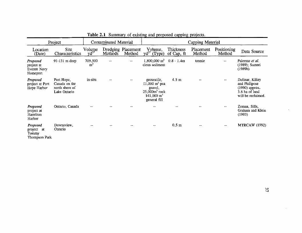
Table 2.1 Summary of existing and proposed capping projects.

Project Contaminated Material Capping Material

Location Site Volume(Date) Characteristics yd3*

Dredging Placement Volume, Thickness Methods Method yd3* (Type) of Cap, ft

PlacementMethod

PositioningMethod Data Source

Proposed project at Everett Navy Homeport

Proposed project at Port Hope Harbor

Proposed project at Hamilton Harbor

Proposed project at TommyThompson Park

91-131 m deep

Port Hope, Canada on the north shore of Lake Ontario

Ontario, Canada

Downsview,Ontario

709,500m3

in-situ

1,800,000 m3 0 . 8 -1.4m clean sediment

geotextile,11,000 m3 pea

gravel, 25,000m3 rock

141,000 m3 general fill

4.5 m

0.5 m

tremie Palermo et al.(1989); Sumeri (1989b)

Dolinar, Killey and Philipose(1990) approx.3.6 ha of land will be reclaimed.

Zeman, Sills, Graham and Klein (1993)

MTRCAW (1992)

38

The migration of metals in sediments is more complex than that for hydrophobic

organic chemicals because several additional factors affect the chemistry of

metals. Most importantly, the oxidation state influences the solubility of the metal and

affinity for the stationary sediment matrix. Thus the Eh, pH, bacterial activity, and

presence of various other nonmetallic species (sulfides, chlorides, carbonates) all

influence metal migration. Brannon, Plumb and Smith (1980) present detailed studies

of the migration of metals from 16 different sites. Due to the complexity of sediment

chemistry with regard to metal migration, the work presented in this document focuses

primarily on the containment of neutral hydrophobic organic chemicals which is

enhanced by finer, higher organic carbon content material.

A potentially significant advantage of sandy cap material, however, is that the

recolonization by the benthic infauna will be primarily suspension feeders as opposed

to burrowing organisms (Cullinane et al., 1990; Morton, 1989; Myers, 1979). This

suggests the possibility of a layered cap in cases where both chemical containment and

bioturbation are important. A lower layer of silty cap material (for chemical

containment) with a sandy layer above (to encourage suspension feeders as opposed to

burrowing animals) might be very effective as a cap.

For a cap to remain unbroken during consolidation, it must be denser than the

underlying material, and the shear stress along the interface between the sediments must

be greater than the strength of the deposit (Semonian, 1981). However, Cullinane et al.

(1990) express concern that mixing of the cap and contaminated sediment may occur

if the cap is denser or coarser than the underlying sediment. A number of

39

investigations have shown that mixing of the cap with the contaminated sediment is not

significant (Mansky, 1984a, 1984c; Bokuniewicz, 1989; Bruin, Hattem and Wijnen,

1985).

§2.3.5 Placement technique. In this subsection we discuss the placement of both

contaminated dredged material (for LBC and CAD) and clean capping material (for in-

situ capping as well as LBC and CAD). Placement procedures are driven by different

concerns for these processes, but the equipment used is the same. There exist two

basic methods for placement of either contaminated dredged material or clean capping

material (Truitt, 1987b): l)modified surface release, 2) submerged discharge.

Sanderson and McKnight (1986) and Palermo (1991b) survey equipment and

construction techniques for capping projects. Zappi and Hayes (1991) present an

overview of dredging technologies for removal of contaminated sediments. Hayes,

McLellan and Truitt (1988) report on dredging equipment demonstrations.

§2.3.5.1 Considerations fo r contaminated material placement. Control of water

column effects arising during dredging and the subsequent placement of contaminated

dredged material is important for remote capping operations as is the creation of an

easily capped configuration of the material on the bottom. In general, minimizing water

column dispersion and bottom spread is desirable. The mixing and dispersion character

of the sediment are closely related to the equipment used to dredge it. Different

techniques are suitable to different sediment types. Cohesion of the dredged material

is the principal controlling factor for water column dispersion (Bokuniewicz and

Gordon, 1980; Morton, 1983a, 1983b). In general, material dredged mechanically by

40

clamshell will maintain its cohesiveness as it falls to the bottom (Bokuniewicz and

Gordon, 1980). Two beneficial results arise: 1) less water column dispersion occurs and

2) a tighter mound configuration usually results. Thus, for the placement of

contaminated sediment clamshell methods may be the most appropriate. If other

considerations suggest that hydraulic dredging techniques are required, then analysis of

the dispersion and spreading may lead to the implementation of additional control

measures such as submerged discharge or CAD. Baldwin, Irish and Bokuniewicz (1990)

discuss the real-time remote monitoring of the mounding and spreading of dredged

material as it is deposited, (see also §2.3.6)

§2.3.5.2 Considerations fo r cap material placement. Specific considerations for

cap placement include the rate of placement, accurate positioning of the cap and

achieving the design cap thickness. Placement methods which disturb the underlying

contaminated sediment by displacement or mixing should be avoided. Large clods,

present in mechanically dredged material (clamshell) may break upon impact with the

bottom and probably would cause significant dispersal and mixing of the underlying

contaminated sediment. Normally, water column effects are not critical in considering

the placement method for the cap material. A possible exception would be potential

adverse effects of a turbidity cloud.

Several studies have shown that careful use of standard dredging equipment will

result in satisfactory cap placement without significant mixing or dispersal of the

contaminated sediment layer (Bruin et al., 1985; Mansky, 1984a; Sumeri, 1991). A

number of different placement techniques may be feasible for a given capping project.

41

If water column dispersion and bottom spread are considered acceptable, (§2.3.5.1)

conventional discharge via barge release of mechanically dredged material can be

considered. For reduction in water column dispersion and additional control in the

placement of the material, some form of submerged discharge may need to be

considered.

The accurate placement of both the dredged material and cap material is an

essential feature of any project (Palermo, 1991a). Truitt (1986) present volumetric and

mass balance estimates for the placement of cap material based on side scan sonar and

hydrographic surveys. Error analysis indicated 8-10% difference in computed values.

It is noted that in busy harbors noise pollution may affect the side scan sonar

results/interpretation. The two basic methods for cap placement are briefly discussed

below.

§2.3.5.3 Modified surface release. Conventional equipment can be used for

contaminated sediment or cap placement, often with only minor modifications.

Dredged material released at the water surface tends to descend to the bottom as a

dense jet with little mixing of water (Bokuniewicz et al. , 1978). Thus it seems an ideal

method for placement of contaminated dredged material; however, surface release of

cohesive cap material is not recommended because of the potential for displacement or

mixing of possibly soft contaminated sediment. Slow sprinkling of sand from a split-

hull barge has worked well (Kikegawa, 1983; Sumeri and Romberg, 1991; Sumeri,

1991; Sumeri, 1984; Truitt, 1986). An impingement plate or sand box may be used to

reduce the discharge energy of dredged material hydraulically discharged at the surface.

42

The dispersion of the material during descent can be modeled with the DUMP model,

which is part of the ADDAMS suite of models used to support ocean dumping

operations (US EPA, 1991)

§2.3.5.4 Submerged discharge. In this method some form of closed conduit is

used to transfer the cap material from the barge hopper to a point near the bottom

sediment. The objective of this technique is to reduce or eliminate any effect of water

current on the cap placement accuracy. This technique also reduces or eliminates water

column dispersion effects. Methods of submerged discharge include: submerged

diffuser (d’Angremond et al. , 1984; Kikegawa, 1983; Kleinbloesem and Weijde, 1983;

McLellan and Truitt, 1986; Lukjanowicz et al. , 1988; Toa Construction, 1990), gravity

downpipe (tremie) (Togashi, 1983; Palermo et al. , 1989), and hopper barge pumpdown.

The primary difference between the first two of these methods is that the diffuser

includes an expansion region and an impingement plate which are designed to reduce

the velocity of the material being placed and thus further reduce the opportunity for

mixing and dispersal of the material being covered. With hopper barge pumpdown, the

normal operation of the barge is reversed and the material is pumped out through the

dredgehead. The dredgehead should serve the same function as a diffuser; however,

the maximum placement depth is limited to the maximum dredge depth of the barge.

Another method was tested at the Rotterdam Harbor. At that site some of the

cap material was a cohesive clay. Since the contaminated sediment was hydraulically

placed and unconsolidated, the clay was dumped next to the site and dragged over the

43

contaminated sediment. This method is not recommended because of increased

resuspension of the sediment (Truitt, 1987a).

§2.3.5.5 Geotextiles. Little has been done using geotextiles as an aid to containing

the contaminated sediment during addition of the cap layer. Dolinar et al. (1990) found

that woven materials were easily clogged which would help minimize mixing of cap and

sediment materials, but could also interfere with sediment consolidation. Geotextiles

were also tested in Rotterdam harbor, but the final design did not include the use of

geotextiles (Bruin et al., 1985). Townsend et.al. (1989) also experimented with

geotextiles although their application was not subaqueous sediments.

§2.3.5.6 Navigation and positioning. In the cases where cap demonstrations were

not judged complete successes, the difficulties were traced to inaccurate positioning and

not equipment flaws (Truitt et a l , 1989). Science Applications International

Corporation (1990) report on a precision bathymetric survey conducted immediately

following cap placement and found that one location designated to receive the most cap

material in fact had less than half the intended thickness. They recommend additional

cap material be deposited, but that better navigational control be incorporated during

the cap placement. A number of navigation aids have been used to aid in the accurate

placement of both dredged material and cap material. These include real-time

computer-assisted helmsmen’s aids, taut moored buoys (Randall and Palermo, 1990),

acoustical positioning devices, and mooring barges (Palermo, 1991b). Sumeri (1991)

and Randall and Palermo (1990) describe computer monitoring of a sand sprinkling

operation using pressure transducers to aid in the determination of the rate of sand

44

discharge from a split hull barge and a shore based laser positioning system to track the

barge; the operation was deemed successful.

§2.3.6 Evaluate spread, mounding, consolidation, and erodability. The amount

of cap material required will depend on the shape of the contaminated dredged material

mound or the aerial extent of contamination for in-situ projects. A more compact

mound configuration will require less cap material. In LBC the dredged material

mound configuration is primarily dependent on the physical properties of the sediment

(§2.3.2 and §2.3.4). Johnson (1990) presents a numerical model for predicting the

initial mound configuration of a dredged material disposal mound (also included in US

EPA, 1991). Lateral spreading can be reduced by placing the contaminated dredged

material in subaqueous depressions (natural or dredged) or behind berms. This would

be considered a CAD facility.

Consolidation of both the contaminated dredged material and capping material

will lead to a more stable deposit. However, it will also result in decreased cap

thickness. Therefore estimates of the degree of consolidation are needed in order to

assure that the required cap thickness is maintained. Truitt (1986) found that 75% of

the consolidation occurred within the first week of cap placement. Poindexter-Rollins

(1990) presents a method for predicting the consolidation of subaqueous sediment

mounds. This is also part of the AD DAMS suite of models mentioned previously (US

EPA, 1991).

Consolidation and the resulting seepage of water from the contaminated sediment

layer might reduce the chemical containment afforded by the cap. If the cap had

45

significant sorptive capacity, however, the movement of the contaminants would be

highly retarded compared to the movement of the pore-water. Thibodeaux and

Bosworth (1990) estimated that Polychlorinated Biphenyls in contaminated New Bedford

Harbor sediments would penetrate only 1 millimeter into a cap with 1 % organic carbon

during primary consolidation.

An analysis of the erodability of the deposit will help determine the extent of

armoring required.

§2.3.7 Determining the required cap thickness. Chemical and biological

characteristics of the contaminated sediment and cap sediment must be considered in

designing the cap thickness. Typically, a certain thickness is required for chemical

containment and an additional layer is required to mitigate the effects of bioturbation

and reduce the potential for bioaccumulation. The bioturbation depth required for a

specific site depends entirely on the naturally occurring species which are likely to

recoIonize the cap site. If for example deep burrowing animals are present additional

cap material will be required.

The US Army Engineer Waterway Experiment Station (USACE-WES) has

developed a laboratory procedure for determining the thickness of a cap required to

chemically isolate a contaminated sediment (Sturgis and Gunnison, 1988a). It is based

on the use of small scale (22 .61) reactors. The significant advantage of this method is

in providing site specific information regarding the effect of bioturbation. Briefly, a

contaminated sediment is placed in the reactor and capped with a certain thickness of

a proposed capping sediment. Following cap addition, bioturbating organisms are

46

introduced to the system. The overlying water concentration of dissolved oxygen,

ammonium-nitrogen and orthophosphate-phosphorous is monitored as a function of time

for both capped contaminated sediment and the capping material alone. The reduction

in sediment oxygen demand or the release rate of either of the other two tracers from

the capped contaminated sediment is compared to that for the cap alone. The cap is

considered to be thick enough if no difference is noted between the control and

experimental treatment. It is important that more than one of the tracers be used in this

test since it is possible, for example, that both the cap and contaminated sediment have

the same oxygen demand and then no reduction in sediment oxygen demand would be

observed.

The reactors used for this test have also been used in a number of other studies

both with and without bioturbating organisms (Brannon et al., 1985, 1986; Brannon,

Hoeppel and Gunnison, 1987; Gunnison et al., 1980, 1987a, 1987b; Sturgis and

Gunnison, 1988b). Wang et al. (1991) have presented laboratory and simple

mathematical simulations of the time dependent rate of hydrophobic organic chemical

release through cap material. The modeling in this paper imposed strict assumptions

regarding the system conditions, specifically that the contaminated layer contaminant

concentration remain constant for all time — clearly not valid in most situations. Horie

(1987, 1991) modeled the effect of capping nutrient rich sediments, following seasonal

changes in dissolved oxygen levels.

Field, laboratory, and model analysis have suggested that the rate of bioturbation

transport is rapid compared to the transport through the underlying non-bioturbed

47

material. The effective cap thickness is generally the total cap thickness minus the

depth of penetration of significant bioturbation activity. The flux through the cap is

initially a function of the effective cap thickness and its sorptive capacity. Ultimately,

however, quasi-steady conditions are likely to exist in the cap and the flux would no

longer be influenced by sorptive capacity, but would be controlled only by the effective

cap thickness. For compounds which are degraded in the anaerobic conditions fostered

beneath a cap, the cap sorptive capacity will affect the ultimate quasi-steady release rate

due to loss of the chemical over time.

Because most contaminated sediment sites include highly hydrophobic

compounds, the design of caps for chemical containment requires an understanding of

the dynamics of these materials. The USAGE-WES reactor based method for

determining the required cap thickness uses non-sorbing tracers. My work has been

aimed at filling the knowledge gaps regarding cap effectiveness at isolating very

hydrophobic contaminants. The effects of sorption in the cap are increasingly important

for increasingly hydrophobic materials, and the extension of laboratory simulations to

include this type of compound is necessary to quantify cap effectiveness. The reactor

method for determining the required cap thickness developed at USACE-WES did not

include any theoretical treatment, and thus has no predictive or general design

capability. In §4.1.5 I have extended the initial theoretical development of Wang et al.

(1991), relaxing the imposed conditions. The advantage of coupling mathematical

design equations with the laboratory simulations is that longer term behavior of the

48

system can be simulated mathematically than is possible in the laboratory, while the

laboratory simulations provide a check on the mathematical predictions.

§2,3.8 Developing a monitoring program . Pre-construction monitoring provides

baseline information to assess the placement of the contaminated sediment and cap

material. Construction monitoring is necessary to assure accurate placement of the

sediment, to assess resuspension of contaminated sediment caused by the operation and

to provide accounting for the volumes of sediment handled (Truitt et al. , 1989; Truitt,

1987b).

A regularly scheduled long-term monitoring program is also necessary to

determine the effectiveness of the cap and should include physical, chemical and

biological monitoring. Truitt et al. (1989) present a tiered approach to monitoring.

§2.3.8.1 Physical monitoring. Techniques covering broad areas (bathymetry, side

scan sonar, subbottom profiles) are combined with direct measurements (cores, grab

samples, sediment profiling cameras, sediment traps, current meters, and reference

rods) are utilized in physical monitoring (Truitt, 1986; Truitt et al., 1989; Science

Applications International Corporation, 1990). Activities included in the long-term

monitoring are bathymetry and sediment cores to assess consolidation (Brandes, Silva

and Fredette, 1991; Brannon and Poindexter-Rollins, 1990), cap thickness and chemical

containment. Monitoring tests should also be performed following specified-threshold

storm or ship events to assess the need for maintenance of the cap. A study on the

effect of storms on cap stability indicated that no large changes occurred even

49

during a hurricane in approximately 20 m water in Central Long Island Sound

(Bokuniewicz et al., 1977).

§2.3.8.2 Chemical monitoring. Post capping cores should be analyzed for

chemical concentration profiles to aid in assessing chemical containment (Sumeri and

Romberg, 1991). Water samples can also be used to assess the chemical containment,

and form the basis for the primary design criterion for cap thickness. Atwell and

Colwell (1981) noted that dredged material associated bacteria are contained beneath

the cap. Parametrix (1990a) monitored CO and methane release from a capped

sediment deposit in Puget Sound and found no evidence of chemical transport by this

mechanism at that site.

§2.3.8.3 Biological monitoring. One aim of biological monitoring is to evaluate

the effectiveness of the cap at isolating the benthic and pelagic communities from the

contaminants of concern. (Mansky, 1984a, 1984c). A bioaccumulation study at the New

York Bight Apex was inconclusive, with the blue mussel (Mytilus edulis) exhibiting

erratic uptake (O’Connor and O ’Connor, 1983). O’Comior and O ’Connor (1983) state

"... sediments, whether capped or uncapped, in place or recently disposed, rarely cause

elevated contaminant levels in natural or implanted biota." It is thought that particle

bound or insoluble forms are simply not bioavailable. (see references in O ’Connor and

O ’Connor, 1983). The IJSEPA (1989) presents compelling evidence that the

bioavailability and associated toxicity (measured by % survival or body burden) of

sediment associated nonionic organic pollutants to benthic organisms is strongly and

directly correlated with the chemical pore-water concentration (which is related to its

50

aqueous phase chemical activity). For metals the strongest correlation is with the

divalent ion activity, [Me+2]. Recolonization of the capped deposit is also important to

monitor as a means of assessing potential breach of the cap by deep burrowing

organisms (Parametrix, 1990b). McCall (1977) presents detailed results from a

recolonization experiment in Long Island Sound.

§2.4 Summary

Review of the available literature points to incomplete understanding of the role

of natural colloids in the transport of hydrophobic chemicals in sediments. The nature

of the transport of the colloids themselves is not completely clear due to inconsistencies

in the initial experimental data (§2.2.2). While colloids have been implicated in

groundwater contaminant transport, little experimental evidence of their effect in

sediment systems is available. My work begins to answer some of the remaining

questions regarding the role of colloids in sediment contaminant transport, providing

consistent data regarding DOC transport (§5.2.1) and preliminary confirmation of a

simple enhanced transport model (§4.2).

The available information regarding capping focuses primarily on the

engineering application of this technology, and not on providing design guidance based

on an understanding of the chemical transport phenomena in sediments. The laboratory

scale work to date has demonstrated the efficacy and some limitations of capping, but,

except for the work of Wang et al.{ 1991), no modeling has been attempted. I have

extended the initial modeling by relaxation of some of the conditions and inclusion of

boundary layer effects (§4.1.1.1) and biodegradation (Appendix D). I have also

performed experiments using hydrophobic contaminants with the aim of providing data

to evaluate the mathematical models, extending the database begun with Wang et a l.,

Chapter 3 Materials and Methods

Laboratory investigations were conducted in three separate areas. These were

1) studies of diffusive transport of contaminants from sediments, both capped and

uncapped, 2) studies of the transport properties of natural DOC, and 3) experiments to

investigate the magnitude of contaminant flux enhancement due to the presence of

DOC. This chapter has been divided into three main sections each focusing on one of

these aspects.

A primary project objective was development and laboratory verification of

simple mathematical models which describe the dynamics of diffusive contaminant loss

from bed sediments, both capped and uncapped. The practical benefit of this effort will

be to enhance the ability to engineer capping layers which will provide effective

chemical containment. This chapter describes the laboratory scale experimental work

performed. The associated analytical and quality assurance procedures are presented

as Appendix A. A note on terminology: the terms analyte, tracer, contaminant, and

pollutant may be regarded as synonymous in the following discussions.

§3.1 Studies of contaminant release

The major focus of these experiments was evaluation of capping as a control

technology for contaminated sediment remediation. The overall approach was to

inoculate sediment with a surrogate contaminant, and then monitor the concentration of

the surrogate in the effluent of a flow-through cell. Uncapped cells were included as

52

53

controls to provide a basis for comparison. Experimental treatments designed to

elucidate the effect of cap properties on the release rate of chemicals from capped

contaminated sediments were performed. Important cap properties affecting the release

rate include porosity, bulk density, organic carbon content, and thickness. In addition,

the total quantity of the contaminant present in the original system should affect the

release rate. Qualitative consideration of the release through a cap can provide insight

into the anticipated effect of each of these factors. Immediately after cap placement the

release rate of a chemical from a contaminated sediment should be very small or

eliminated since some time will be required for the chemical to traverse the cap

(breakthrough time). Additionally, if the water column is continually flushed, the

chemical potential gradient will always favor transport to the water, and ultimately the

chemical should be completely removed from the sediment. At some intermediate time

then, the release rate must pass through a maximum value. The long-term rate at

which the flux approaches zero will be controlled by the depletion rate of the

contaminant from the sediment (either by degradation or loss to the water column). It

is reasonable to believe this should be manifest in the flux vs. time profile after the

maximum flux has been reached. Increasing the cap depth should increase the chemical

containment effectiveness of the cap by lengthening the breakthrough time and reducing

the maximum release rate; both these effects are the result of increased path length.

Increasing the organic carbon content of the cap should increase the breakthrough time

without affecting the long-term release rate (provided depletion of the compound is

minimal - if a significant fraction of the contaminant is ‘stored’ in the cap the long-term

54

release rate should be less). These hypotheses were experimentally tested. A number

of materials and property measurements are required for the execution and analysis of

these experiments. The following subsections present sediment selection and

characterization, physico-chemical property measurement, and the experimental setup

including data collection procedures.

§3.1.1 Sediments. Sediments from four sites and quartz sand were collected and

characterized. No effort was made to collect sediment samples characteristic of a given

source or geographical region. The sediments were collected from University Lake

(Baton Rouge, LA), Bayou Manchac (Baton Rouge), Cocodrie (Cocodrie, LA; an

estuarine sediment) and Lake Pontchartrain (Mandeville, LA). In addition quartz sand

from a local aggregate supplier was used (this stock was on hand from previous

student’s work). The sediments were chosen to represent a range of physical

properties.

These sediments were used both as uncontaminated cap sediments and inoculated

(artificial) contaminated sediments in the laboratory capping simulations and also for

the DOC transport studies. University lake sediment was used as the inoculated

sediment because of its relatively high organic carbon content.

§3.1.1.1 Sediment preparation. After collection from the field the sediments were

processed. The first step was coarse sieving (3/8" mesh) for removal of twigs, leaves,

etc; followed by fine sieving (#14 sieve: 1.41 mm openings) for removal of larger

pebbles, rocks, etc; and finally, for the first series of sediments, air drying. The air dry

sediments were stored in metal buckets with lids (not air tight).

55

§3.1.1.2 Characterization. The sediments were characterized by organic carbon

content, sand, silt and clay fractions, porosity, bulk density, particle density, and cation

exchange capacity. Standard methods were followed and are described in Appendix A.

Bulk density and porosity measurements were made for the sediments as placed in the

CSCs. The sediment properties are reported in Table 3.1.

Table 3.1 Sediment physical properties

Sediment

a.fAoc bPP

g/cm3cP b

g/cm3de %

Sand%Silt

%Clay

eCECmeq/lOOg

UL 0.041 2.5 0.886 0.65 10 76 14 3.99

PON-R1 0.008 2.5 1.35 0.46 10.4

PON-R2 0.008 2.5 1.57 0.37

QS 0.0005 2.68 1.39 0.48 0.17

ULF-Rl

0.035 2.3 0.64 0.72

ULW -Rl

0.045f 2.3 0.62 0.73

BayouManchac

0.021 2.44 1.0 0.59 29 37 34

ULF-R2

0.039 2.35 0.72 0.69

ULW-R2

0.04 2.35 0.76 0.68

a fraction organic carbon; b particle density; c bulk density; d porosity; e cation exchange capacity; f this sediment had residual dye used as a tracer in another student’s work. No analytical interference was observed, but the dye may be the cause of the higher carbon content of this sediment.

56

§3.1.2 T racer selection. I chose to use poly aromatic hydrocarbons (PAHs) as the

primary tracers in this work because of their chemical neutrality and stability and

relatively low Henry’s constants and vapor pressures. In addition, these compounds are

ubiquitous contaminants in the environment (e.g. Readman et al. , 1987; Martel et al.,

1986). The specific compounds used as tracers were dibenzofuran, phenanthrene,

fluoranthene and pyrene. Anthracene was used as a surrogate for spiking in some of the

quality assurance testing. Although dibenzofuran is not classified as a PAH, the

extraction and chromatographic methods for PAHs are very effective for this compound

as well (see Appendix B). The chemical properties of these compounds are given in

Table 3.2, and their structures are shown in Figure 3.1.

Table 3.2 PAH physico-chemical properties

Property PhenanthreneCompound

Fluoranthene Pyrene Dibenzofuran

Xmax nm Water

252 237 240 217

Solubilitymg/L

1 0.26 0.15 10

Log Koc 4.4 4.6 4.8 4±0 .1Log Kow Henry’s

4.5 5.2 5.1 4.15

Constant atm • nrVmol

Waterdiffusivity

6.0 x 10 5 1.8 x lO'2 1.0 x 10 s 7.9 x lO'5

(20°C)cm2/s

5.8 x 10‘6 5.3 x 10'6 5.5 x lO 6 6.0 x lO'6

57

Phenanthrene CAS#: 85-01-8 MW: 178.24 Formula: CJ4H 10

AnthraceneCAS#: 120-11-7 MW: 178.24 Formula: C ]4H 1Q

Dibenzofuran CAS#: 192-64-9 MW: 168.20 Formula: C H ,o

Fluoranthene CAS#: 206-44-0 MW: 202.26 Formula: C 16H 10

PyreneCAS#: 129-00-0 MW: 202.26 Formula: C ,,Hlo 10

Figure 3.1 PAH chemical structures

§3.1.3 Partition coefficients. One of the most important parameters in determining

the dynamics of hydrophobic compounds in soil/sediment systems is the partition

coefficient between the sediment and adjacent pore-water. I used a batch equilibration

method for measuring the partition coefficient of each of the tracers used in this work

to the sediments. The partitioning of pyrene to University lake was performed with

pyrene as the only tracer in the system. All of the other partition coefficients were

obtained from assays in which there were either 3 or 4 chemicals present. Two or three

grams (exact weight recorded for calculations) of air dried sediment was placed in a

100 mL crimp top vial (Supelco, Inc.) and 100 mL of water was added to suspend the

sediment. The PAHs were spiked into the system from a concentrated stock solution

58

in acetonitrile. Where possible the volume fraction of acetonitrile in the system was

kept below 0.1% (always below 0.3%) to prevent co-solvent effects from influencing

the measured partition coefficients. The vials were crimp sealed with teflon lined septa

and placed on an end over end shaker for 4 days. The vials were then opened and the

contents transferred to centrifuge bottles. Phase separation was effected by

centrifugation at 13,000 rpm for 30 minutes (IEC B20 centrifuge). An aliquot of the

supernatant was removed by pipette and extracted with hexane following the procedure

detailed in Appendix A.3.1.

§3.1.4 Sediment inoculation. The inoculation procedure required two steps. The

first was plating the tracers on the wall of an inoculation vessel (1 gallon glass jar), and

the second was tumbling the sediment in the vessel.

The tracers were plated on the inside wall of the inoculation vessel by first

dissolving the tracers in hexane and then transferring the hexane solution to the

inoculation vessel. Finally, the hexane was evaporated under a stream of ultra high

purity nitrogen while rotating the inoculation vessel. This resulted in a uniform

deposition of the tracer crystals on the vessel wall which appeared quite stable. The

sediment slurry (2 kg dry weight @ 60 %w water dosed with 400 ppm sodium azide to

eliminate bioactivity) was then placed into the inoculation vessel and tumbled (axial

rotation at a rate of 5-10 rpm) for 10-14 days (Means et al., 1980; Karickhoff and

Morris, 1985). The sediment inoculation levels, both target level and measured level,

are reported in Table 3.4.

59

After inoculation but prior to loading the sediment into the simulators, the

sediment was allowed to settle, and the excess water was removed until the consistency

was sufficient to support the cap material. Prior to or during the first days of the run,

the inoculation level (sediment loading) and pore water concentrations of the tracers

were measured by soxhlet extraction (solid samples) and liquid-liquid extraction (pore-

water). The methods are discussed in detail in Appendix A. The pore water sample

was obtained by centrifugation (15,000 rpm for 30 min) of a subsample of the

inoculated sediment in a fashion similar to that used for partition constant determination

(Appendix A .3.1.3).

§3.1.5 Experim ental apparatus. The experiments were conducted in a capping

simulator cell (CSC) designed to study sorption-retarded diffusion of chemicals from

contaminated sediment on a laboratory scale (Wang et al. , 1991).

The CSC was constructed from !4 inch aluminum. The device, shown in

Figure 3.2, was a flow cell consisting of two chambers and a removable glass lid. The

two chambers bolt together, and complete sealing was effected by silicone grease.

Silicone grease was also used to seal a glass lid onto the top of each simulator. The

lower chamber contained the inoculated sediment and the top chamber contained the cap

layer and overlying water. As shown in Figure 3.2, the exposed sediment area was

75 cm2. Each CSC required approximately 150 g of contaminated sediment and 20-50 g

for the cap depending on the cap thickness. Options for determining the thickness of

the cap and contaminated layers include a 5.8 mm thick spacer (allowing thicker caps)

and a molded insert for the bottom section (allowing thinner caps).

Sideview a

37.3mm skimmer bladeB

/

5.8 mm optional spacer

15 cm

Planview o q 5 cm

Figure 3.2 Schematic of the simulators used in this study. Dimensions for each simulator are given in Appendix F

§3.1.6 Sim ulator loading and operation. In preparation for an experimental run,

the bottom chamber was filled with contaminated sediment as a thick slurry and leveled

with a spatula. The top chamber was then bolted on. Mixing of the layers was kept

to a minimum by careful placement of the cap layer on the contaminated sediment.

Prior to cap placement stagnant water was removed by a pasteur pipette. In field

applications, there will probably be pockets of water between the cap and contaminated

sediment. However, the sediment will consolidate over a relatively short time period

(compared to the expected life of such a facility) and the water pockets will be

incorporated into the pore waters. Thus the removal of water from the sediment prior

to cap placement was an attempt to simulate the system after the initial consolidation

61

— which is the state important in determining the long term effectiveness of the

technology. The cap sediment was then spread over the contaminated sediment and

leveled using a machined skimmer. The cap thickness was determined by the use of

either a spacer between the chambers which caused the total sediment depth to be

greater for these cells (thick cap) or an insert in the bottom chamber which increased

the contaminated layer depth while keeping the entire sediment depth constant (thin cap)

in conjunction with skimmer as shown in Figure 3.2. This procedure, as opposed to

using different skimmers, minimizes the variation in the water depth above the cap,

which reduces the experimental variability introduced by water side resistances. The

tolerance for sediment depth was ± 1 mm. Cap thicknesses of approximately 3 mm

(for high organic carbon caps) and 7 and 13 mm (for low organic carbon caps) were

chosen in order to have reasonable breakthrough times (on the order of 3 to 30 days).

Continuous water flow across the CSC was provided using a ten channel

peristaltic pump (Manostat 519) with a capacity from 5 to 75 ml/hour; the actual

average flowrate for each cell in each experimental run has been given in the previous

sections. The flow was measured for each channel by timing the collection of the

effluent sample scheduled for analysis. That is, the effluent from the simulator was

collected for a measured time interval, T, from each CSC into a tared receiving bottle.

The volume collected, V, was determined by weight with the assumption that the

density of the solution was 1 g/cm3 (Ohaus 400 g +0.01 g). Flow rate was calculated

by: F = V/T. Figure 3.3 shows the experimental setup used for the capping runs.

62

Float

10 channel peristaltic pump

20 L carboy

400 ppm sodium azide

Recirculatingconstanttem perature water bath

W ater bath

Levelingtable

Collectionbottle

Figure 3.3 Experimental setup for capping experiments

During the simulation experiments, all outflow scheduled for analysis was

collected as a composite sample in a collection vessel connected to the exit of the CSC.

The connection was via glass tubing through a teflon lined septum. The only

connection to the atmosphere was a needle through the septum which allowed air to

escape as the bottle filled. In conjunction with the glass covers, this sample collection

scheme minimizes the opportunity for evaporative losses of the tracers. Evaporative

losses would cause an artificially low measured flux since the flux is inferred from the

measured water concentration in the effluent. Composite samples for tracer analysis

were collected for 6-18 hours in order to assure adequate sample volume for the

63

extraction procedure (the minimum sample volume was 50 mL). The sample initiation

and collection time and date was kept as part of the data record. Effluent samples were

collected at intervals varying from daily to weekly.

§3.1.7 Experimental design. As mentioned above, the basic measurements for

these experiments were the effluent flowrate and concentration from which the flux can

be inferred. Two runs were conducted, each consisted of ten CSCs. There were four

experimental treatments and an uncapped control. Each treatment and the control were

duplicated in each ten cell run.

The experimental conditions for each of the cap runs are presented in Tables 3.3

& 3.4. The variables which could be manipulated in this system were the sediment

contaminant load (inoculation level), water flowrate, cap thickness, and the cap material

(indirectly changes the partition coefficient). Although the flowrate was different in the

two cap runs, the effect of water side resistance to mass transfer is not expected to be

significant under most field conditions and was not an experimental focus in this study.

Nevertheless, in the laboratory, water-side resistance may be significant and therefore,

it is considered theoretically in §4.1.1.1, and water-side mass transfer coefficients were

calculated from experimental fluxes obtained from the uncapped control cells (§5.4).

The first run was designed to test the one layer model developed in §4.1.4 by

inoculating the contaminated sediment layer above its critical loading (defined in

§4.1.1). The second run included two additional tracers at inoculation levels

approximately 10% and 80% (dibenzofuran and phenanthrene resp.) of their critical

loading. The primary data collected in each run was the tracer concentration of the

64

Table 3.3 Experimental conditions for cap run 1

Sediment Inoculation: August 1991 Start of run : 4/4/92 End of run: 7/17/92

CSCs for both runs placed in a water bath at 20±°C

Cap Contaminated Avg. FlowCap3 depth layer depth (ml/hr)

Cell (cm) (cm) first 80 days final 23 daysb

A Pon 0.341 1.849 6.6+1.3 14.6+3.2

B Pon 0.301 1.849 6.3 + 1.1 13.8+3.0

C - - 2.196 6.6 + 1.2 14.6+3.2

D QS 0.715 1.476 7.2 + 1.4 15.8+3.5

E QS 0.720 1.460 6.8 + 1.3 15.0+3.3

F QS 0.722 1.468 6.9 + 1.4 15.2+3.5

G QS 0.768 1.422 6.6 + 1.3 14.3+3.3

H - - 2.191 6.5 + 1.2 14.8+3.3

I Pon 0.336 1.854 6.8 + 1.3 14.7+3.1

J Pon 0.348 1.842 6.4 + 1.2 14.3+3.2a Pon == Lake Pontchartrain sediment; QS = quartz sand.b flowrate intentionally increased

Initial tracer loading

Pore-water Sediment(ng/L) (mg/kg)

Chemical measured target measured

Pyrene 120.0 2000 2009+90(n=2)

effluent collected from the CSCs. In conjunction with the measured flowrate, this

allowed the release rate of the tracer to be calculated. This information was used to

assess mathematical models of the system dynamics (Chapter 6).

65

Table 3.4 Experimental conditions for cap run 2

Sediment Inoculation: 06/30/92 - 7/15/92 Start of run : 10/08/92 End of run: 4/28/93

CSCs for both runs placed in a water bath at 20±°C

Cell Cap3 Cap depth (cm)

Contaminated layer depth

(cm)

Avg. Flow (ml/hr)

A Pon 0.347 1.849 11.3 + 1.7

B Pon 0.301 1.849 12.2+0.3

C QS 0.733 1.463 12.0+1.0

D QS 0.715 1.476 11.9+0.4

E - - 2.18 12.1+0.3

F - - 2.19 11.9+0.3

G QS 1.382 1.422 11.7+0.3

H QS 1.308 1.463 12.0+0.6

I Pon 0.336 1.854 11.6+0.3

J Pon 0.348 1.842 11.8+0.23 Pon = Lake Pontchartrain sediment; QS = quartz sand.

Initial tracer loading

Chemical

Pore-water(ng/L)

measured target

Sediment(mg/kg)

measured(n=4)

Dibenzofuran 772.4 327 250+39

Phenanthrene 307.8 373 342 + 19

Pyrene 168.0 1045 1170+55

Post mortem coring of the sediment/cap followed by thin sectioning (2 mm) and

analysis of sediment tracer load was performed to determine the in bed concentration

66

profile (§5.4.1.2, 5.4.2.2) for the second run. Mathematical model predictions of the

concentration profile were made using parameter values fitted from the contaminant flux

data. To facilitate core removal each CSC was placed in a freezer for 20 minutes prior

to coring to stiffen the sediment (but NOT freeze minimizing disruption of the

structure) sufficiently to allow easy removal of the core from the CSC.

Sections were obtained by placing the core on a threaded post with a pitch of

2 mm shown in Figure 3.4. The core support was lowered one to five revolutions and

a section cut from the top of the extruded core. Eight to ten sections were taken per

core and up to two cores were taken for each cell. The core sections for contaminant

Stainless steel core used for removing sediment from the simulator

2 mm per revolution pitch

Core support: lowered to extrude sediment core for sectioning with knife & spatula

Position indicator

Figure 3.4 Sectioning device used to obtain sediment profile data

67

analysis were stored frozen in 20 mL screw top vials prior to extraction using the

column method described in Appendix C.

§3.2 Colloid transport studies

The experimental goal for these experiments was to elucidate the transport

properties of natural DOC independent of any effect on the transport of contaminants.

Both Brownian diffusion and advection with pore-water can transport colloids from a

sediment bed to the overlying water. The experiments reported here were undertaken

to clarify the diffusive exchange of DOC between bed sediments and the overlying

water. The experiments were designed to determine the flux of DOC from bed

sediments to overlying water and to study the effect of a sand cap in retarding DOC

release from a sediment bed. The emphasis of the laboratory experiments was on in­

bed sediment processes, since transport between sediment and water is generally

sediment-side controlled.

§3.2.1 Sediments used. The same sediments collected and used for the contaminant

flux experiments described above were used for these experiments. One exception is

that University lake sediment collected during a second ‘field trip’ was used for the

deep bed experiments. The preparation of this sediment also differed from that in the

earlier runs in that it was not air dried, but sieved only and stored in air tight plastic

buckets. The sediment used for the deep bed run was frozen and then thawed prior to

placement in the cell, but not treated with sodium azide. It was thought that freezing

the sediment might cause disruption of the clay matrix freeing occluded organic carbon,

68

thus increasing the available mobile DOC fraction (Means, 1993 personal

communication).

§3.2.2 DOC partitioning. The partition coefficient of DOC between the sediment

and adjacent pore-water is an important parameter in the model of DOC release from

sediments. The following assay was used to measure the partition coefficient. 15 g air

dried sediment was suspended in 80 ml distilled deionized water (DDW), then allowed

to settle for two days prior to removing 60 ml supernatant water for DOC*analysis. A

60 ml aliquot of water was replaced, and the sediment was resuspended by end over

end shaking for 30 to 45 seconds. This procedure was repeated. As the sediment was

washed in this manner, the DOC concentration decreased. A mass balance determined

the amount of carbon remaining in the bottle by assuming that the total sediment mass

multiplied by the fraction organic carbon gave the total organic carbon in the system.

Thus knowing the volume of water and DOC concentration removed at each step, the

quantity of carbon remaining on the sediment was calculated. Regressing the data as an

isotherm of the water vs. sediment concentration yielded the partition coefficient. This

was done for Bayou Manchac and University lake sediment, although only the results

for Bayou Manchac proved useful due to extreme scatter in the University lake data.

§3.2.3 Experim ental apparatus. A preliminary series of experiments was

conducted following the procedures given by Koulermos (1989) in one-liter beakers. A

second series of experiments used flow cells similar to those used for the cap runs

(§3.1.5). The experimental conditions for these runs are given in Table 3.5. The

sediment bed depth was 20.1 mm. One final run was performed using a modified

69

version of the flow through cells. The modification was to include a seven centimeter

lexan spacer between the two chambers (which were then connected with long threaded

rods), thus allowing approximately 10 cm deep sediment columns to be studied with a

flowing water boundary condition at the sediment water interface.

§3.2.4 Experim ental approach. Two indicators of DOC diffusion from the

sediment to the overlying water are the overlying water (effluent) DOC concentration

and the development of a concentration profile in the sediment bed itself. Experiments

designed to detect these indicators were performed.

§3.2.4.1 DOC sediment profiles. In-beaker and flow through cell assays were

performed to measure the development of in-bed DOC profiles in the interstitial water.

The beaker experiments began with approximately 1200 g air dried sediment placed in

a glass gallon jar. One liter of distilled water plus 1 g NaN3 was added to the sediment

and placed on the axial tumbler used for tracer inoculation for 48 hours. The sediment

slurry was transferred to a 1 L beaker to a depth of approximately 10 cm. Replicate

Table 3.5 Experimental conditions for DOC transport experiments

Avg. Flowrate Initial [DOC]

Run ID (mL/day) (mg/L)M592A 168 258

M592B 144 258

M892 180 330

U992 164 280

Deep Bed 253 24

70

beakers were prepared for each sediment, then placed in a 30°C water bath. 20 L of

a stock solution containing 400 ppm NaN3 was prepared and used to exchange the

overlying water every 48 hours. This exchange of the overlying water was intended

to keep the overlying DOC concentration near zero. After 90 and 180 days for

University lake and Lake Pontchartrain sediments and after 74 days for Bayou Manchac

and Cocodrie sediments, the water was completely removed. The sediment was then

cored and sectioned into 1 cm sections. Cores from the DOC beaker experiments were

taken by placing 3 core tubes in the beaker to be cored and then removing sediment

surrounding the cores with a spatula. After this sediment was removed, a flexible

plastic ruler was slid beneath the core and a slight vacuum applied to the top (using a

pipette bulb) and the core was removed and placed on the sectioning device. Each core

section was centrifuged at 15,000 rpm for 30 minutes (IEC B-20 refrigerated centrifuge)

to obtain a pore-water sample, which was filtered through a 0.4 pm filter to obtain the

DOC fraction. The water sample was analyzed on a Shimadzu TOC 500 organic

carbon analyzer (see Appendix A for details).

One run was performed using simulator cells which had been modified to hold

a ten centimeter deep sediment bed. The primary aim of this run was to collect a DOC

sediment profile in a system in which the sediment-water-interface boundary condition

was reasonably constant as opposed to the beaker assays described above. Water was

pumped (10.5 ml/hr) through the simulator for 117 days prior to taking two cores from

a single cell for analysis. For the deep cell flow through profiles, the core tubes were

placed in the simulator, and the simulator was disassembled to allow easy removal of

71

the core for sectioning. 4 mm sections were taken from each core and centrifuged as

above to obtain the pore-water sample; however, the sample volume was too small to

reliably filter. For this reason the sample was directly injected onto the organic carbon

analyzer from the centrifuge tube.

§3.2.4.2 DOC flux to overlying water. These experiments were aimed at

monitoring the release of DOC from sediment beds. For this reason the simulators were

not loaded in stages as was required for the cap runs. Loading the cells was

accomplished by dropping a glob of sediment slurry into the cell and tapping and

spreading it out with a spatula and then leveling the surface with the skimming device

used for the cap studies. In the studies where a sand cap was placed above the sediment

bed the cells were loaded and assembled as described for the cap studies above.

The entire apparatus was placed in a water bath at a temperature of 24.5 +1 °C,

and a continuous flow of water through the system was maintained using a peristaltic

pump (Scientific Industries, Bohemia, New York) (Table 3.5). The outflow from the

simulator was collected in a covered beaker. Composite samples for DOC analysis were

collected for 1/2-12 hours. Effluent samples were collected at intervals varying from

four hour to 4 day intervals for the DOC flux experiments. Sampling time was noted,

and the effluent volume was determined gravimetrically (assuming a density of 1

g/cm3). Subsamples were then filtered through a 0.4 fim PVP-free polycarbonate

membrane filter (Poretics, Livermore, CA). As mentioned previously (§2.2), dissolved

organic carbon (DOC) concentration was considered to be a surrogate measure of the

colloid concentration. The analytical method for DOC concentration determination was

72

platinum catalyzed wet oxidation at 650°C. Details are presented in Appendix A. The

observed DOC release rate is compared to mathematical model predictions in §4.2.

§3.3 Colloid-facilitated contaminant transport

It is believed that contaminant molecules “piggy-back” on natural occurring

colloids in soil and sediment systems. If this is the case then the rate of release of a

contaminant from a system free of colloids should be lower than the release rate from

a system with colloids. The ideal demonstration of this effect would be one in which

the chemical flux from two systems identical except for the level of mobile colloids

were compared. In this demonstration, direct experimental evidence should indicate the

presence or absence of enhanced chemical flux with out the need to make comparisons

through mathematical models of the system dynamics which would be required if there

were significant differences between the systems compared. An attempt, described

below, to make such an experimental comparison was made.

§3.3.1 Sediment p reparation. University lake sediment was used for the colloidal

enhancement experiments. The sediment was collected at a later time than the sediment

used in the capping and colloid transport work described above and was not air dried

after the coarse and fine sieving operations. In an attempt to produce sediments which

were similar in all respects except the available level of mobile colloids, special

preparation of the sediment used was as follows. First the sediment was frozen and

thawed twice. The sediment was then thoroughly mixed and one-half of it was placed

in a large diameter teflon column. Distilled deionized water was pumped through the

73

column for two weeks, and the DOC level in the effluent was monitored. The column

was opened every three or four days, and the sediment was mixed to minimize any

effects of channeling on the efficacy of the sediment washing. The washing was

stopped when the effluent DOC concentration had reached a plateau at a level of

approximately 1.5 ppm. It is apparent that the freezing treatment did not have the

desired effect for the second run; the reason for this is unknown (see Table 3.6).

§3.3.2 Experim ental apparatus. The flow cells used for the capping experiments

described in §3.1.5 were used unmodified for these experiments.

§3.3.3 Sim ulator loading and operation. These experiments were performed using

uncapped sediments and thus did not require that the CSC be loaded in two stages as

for the capped runs. A mound of sediment slurry was placed in the simulator and

spread out with a spatula and finally levelled using the skimming blade described

previously. Continuous flow of distilled deionized water with 400 ppm sodium azide

was maintained through the cells using a Manostat 519 ten channel peristaltic pump.

§3.3.4 Sediment inoculation. The same procedure described in §3.1.4 was used.

Special care was taken to assure that the conditions were identical in each inoculation

vessel (wide mouth 1 liter teflon lined cap jars). Specifically, the moisture content of

each sediment (i.e. washed and frozen) was measured prior to inoculation and the same

dry weight of each was added to the respective inoculation vessel. The tracer stock

solution was prepared in a 50 ml volumetric flask and 20 ml was pipetted into each

inoculation vessel to assure that the total tracer loading for each sediment would be the

same. As the results in Table 3.6 indicate, the sediment loading was nearly the same

Table 3.6 Experimental conditions for colloid enhanced flux runs

74

Run 1 Run 2

CellInitial [DOC] (mg/L)

Flowrate(mL/hr)

Initial [DOC] (mg/L)

Flowrate(mL/hr)

W1 1.5 14.3+0.2 1.8 17.2 + 1.1W2 1.5 14.0+0.2 1.8 17.1 + 1.0FI 22 14.7+0.2 2.8 17.6+0.3F2 22 14.5+0.2 2.8 16.2+0.2

Initial tracer loading - Run 1Sediment

Measured pore- (mg/kg)water

Chemical Washed(Mg/L)

Frozen(Mg/L)

Washed target measured

(n=10)

Frozenmeasured(n=10)

Dibenzofuran 349 447 194 155.5+8.6 172.7+28Phenanthrene 104 130 197 186.5 + 13 200.3 + 13.7

Pyrene 24.3 27 186 185.6 + 14 198.3+9.3

Initial tracer loading - Run 2Measured pore- Sediment

water (mg/kg)

Chemical

Washed(Mg/L)

Frozen(Mg/L)

Washedtarget measured

(n=3)

Frozenmeasured

(n=7)

Dibenzofuran 118 88.9+ 4.2 88.8+4.6PhenanthreneFluoranthene

Not Available77.780.6

62.8 + 1.8 76.2+2.3

63.1+4.577.2+3.1

Pyrene 83.2 76.9 + 1.5 78.5+3.9

in the first run and virtually identical in the second. The sediment loading and pore-

water concentrations were determined as described in §3.1.4.

75

§3.3.5 Experim ental design. The aim of these experiments was to detect

differences in contaminant flux from systems which differed only in the level of

available mobile colloids. Presumably, any difference observed, then, would be the

result of enhanced transport of the contaminant due to the presence of the colloids. Two

experimental runs with tracer inoculated sediment were performed. Each treatment was

conducted in duplicate. The experimental and initial conditions are given in Table 3.6.

The following chapter presents a theoretical development of the dynamics of the

systems studied experimentally.

§3.4 Summary

In this chapter I have presented the experimental outline of my work. There

were three areas of experimental focus. Because of the potential for cost effective

remediation of contaminated sediments through capping, the major focus was the

investigation of capped contaminated sediments. Two experimental runs using 10

simulators each were performed. The primary data collected form these runs was the

effluent chemical concentration which was used to infer the chemical release rate. Post­

mortem cores were taken from the sediment in the second run. These cores were

sectioned and extracted to obtain the sediment concentration profiles of the chemicals

used.

Because diffusion is expected to be the dominant release mechanism after

capping, additional studies on the possible effect of natural organic colloids on the

transport of hydrophobic organic chemicals in sediments were conducted. There were

76

two facets of this work: first, studies on the transport properties of the colloids

themselves, aside from any effect on hydrophobic organic chemical transport; and

second two runs using sediment prepared to enhance the availability of mobile colloids

were performed to directly assess the effect of the colloids on contaminant transport.

Chapter 4 Mathematical Modeling

In this chapter mathematical models of the dynamics of the diffusive transport

of both hydrophobic organic chemicals and naturally occurring organic colloidal

particles are developed.

The purpose of the models is to explore the diffusive transport processes

involved in hydrophobic pollutant release from bed sediments and to provide a starting

point for estimation of pollutant release rates which in turn provide the basis for

exposure and risk assessment and ultimately resource allocation as discussed in

Chapter 1.

The models show generally good agreement with the experimental observations,

indicating that the fundamental transport mechanisms are reasonably modeled. A

sensitivity analysis suggested that the key factors controlling the effectiveness of a cap

at isolating the benthic and pelagic communities from exposure to hydrophobic organic

chemical pollutants are the cap thickness and its organic carbon content. A cap

effectiveness factor is defined and plotted as a function of time and the above

parameters.

§4.1 Modeling contaminant release

Three situations are considered: a base case of uncapped contaminated sediment,

a case associated with short times or high sediment contamination levels in which the

contaminated layer pore-water concentration remains constant, and a more general case

77

78

in which the pore-water concentration of the pollutant in the contaminated sediment

layer decreases with time.

Several parameters are necessary for model implementation. These include the

porosity and bulk density of the sediments, the partition coefficient for the chemical(s)

between the pore-water and the sediment(s), and the molecular diffusivity chemical(s)

in water. Because of the number and the uncertainty associated with the measurement

or estimation of these parameters, the development of complex numerical models is not

presently warranted. The models presented here are simple analytical models based on

pollutant pore-water concentrations. Local equilibrium and linear partitioning for the

pollutant between sediment particles and the aqueous phase is assumed. Explicit

mathematical treatment of the sediment particles is not included, and kinetic effects

associated with desorption from sediment particles are not incorporated into these

models.

§4.1.1 Development of a conceptual model. The capped system is conceptualized

as two finite layers; the cap is initially contaminant free, and the underlying sediment

is uniformly contaminated. Note in the application of these models that the origin (i.e.

z = 0) and positive direction have been chosen differently for mathematical

convenience in the analysis of each case. The focus of this work is diffusive processes

in a cap/sediment system, and hence advective transport, including advective transport

during cap consolidation, is not considered. Thibodeaux and Bosworth (1990) have

estimated, for PCBs in New Bedford Harbor, the depth of chemical penetration into a

79

typical cap during primary consolidation (when the chemical is advected upward) would

be of the order of 1 mm, and should occur in a few months time (Truitt, 1986).

Due to the high sorptive capacity of most sediments in comparison to the water

solubility of many hydrophobic organic chemicals (HOC), the concepts of the solubility

limit and critical loading of contaminated sediment are important (Thibodeaux and

Bosworth, 1990). Linear partitioning of the HOC between the aqueous and sediment

phases is a ssu m e d :^ = KdpA. where ^ is the sediment loading (mg/kg), the

partition coefficient, Kd has units of L/kg and water concentration, pA, has units

mg/L. Linear partitioning can only hold until the aqueous solubility, p* , of the

chemical is reached at the critical sediment loading, = Kdp% • Above this sediment

loading the pore-water concentration remains constant at the chemical solubility.

Different boundary conditions apply at the bottom of the cap layer if > co than if

wa <<0^ as discussed below. Field conditions with co^>o)^ are common.

§4.1.1.1 Sediment-side and water-side resistances to mass transfer. The benthic

boundary layer resistance to mass transfer may be an important factor, particularly in

laboratory simulations. For the uncapped situation with the water side presents

the only mass transfer resistance (in both the field and the lab). To determine the

conditions under which water-side resistances to mass transfer should be incorporated,

first consider an uncapped, uniformly contaminated sediment layer. Comparison of the

mass transfer resistances on each side of the sediment-water interface can be

accomplished through estimates of the mass transfer coefficients.

My purpose here is to estimate the water-side mass transfer coefficient in the

laboratory simulations. It has been shown that the mass transfer coefficient for

dissolution of a (solid) solute into fully developed laminar flow is given by (Kramers

and Kreyger, 1956)

where r = dUx/d z is the velocity gradient at the solid-fluid interface, Dw is the

chemical diffusivity in water (cm2/s), and L the length of the mass transfer region.

Assuming maximum shear stress, x0 , at the solid-fluid interface and a linear decrease

of shear stress, ^ , to the free surface (z=H), the velocity profile above the sediment

surface is

where n is the fluid viscosity. The volumetric flowrate past the surface, q, can be

found from:

with W the width of the dissolving region. For a given flowrate, equations (4-2) and

(4-3) provide a relationship for the velocity gradient, r \ needed in equation (4-1),

giving finally:

(4-1)

(4-2)

(4-3)

kj = 1.165q d :

81

\ l / 3

\ H 2L W ,(4-4)

Clearly, at very short times the water-side resistance will be controlling because

no concentration gradient exists within the sediment. Thus the sediment-side resistance

will increase with time as the sediment is depleted of the chemical and the sediment-

side path length increases. A semi-infinite-domain error-function solution for the

concentration profile (Formica et a l., 1988), which should be valid during the initial

stages of contaminant depletion when any effects of an in-bed boundary will not yet

influence the release rate, can be used as the basis for estimating the sediment-side mass

transfer coefficient. Based on the error function solution, the flux,

Na = d(pA)/dx\ through the sediment-water interface (swi) is given by

Na = pQljD eRf/(iit) where NA is the chemical flux (/xg ■ cm-2 • sec-1), p0 is the initial

pore-water concentration in the contaminated sediment (/xg/cm3), s is the bed porosity

(cm3 water/cm3 total), t is time (sec), />e = Dw(e/x) = Dw e4/3 is an effective difftisivity

which corrects the molecular diffusivity of the chemical in water for the reduced area,

e , and tortuousity, x , of the sediment bed. For a saturated unconsolidated granular

4/3sediment, the tortuousity is approximately e (Millington and Quirk, 1961).

Rj. ~ s + pbKd arises from the accumulation term in the governing differential mass

balance on the immobile (sediment) phase (see §4.1.2), pb is the sediment bulk density

(g/cm3) (Formica et al., 1988). Taking the overall mass transfer resistance, 1IK0, to

82

be the sum of the water-side and sediment resistances, given by \ jk and pQ/NA

respectively yields

1IK0 = l/kt + t)l(DeRf )

A simple calculation using parameters taken from the experimental simulators

described earlier (§3.1.5) and the physico-chemical properties of 2,4,6-trichlorophenol

(Table 6.4) shows that the time for the sediment-side resistances to become equal to the

water-side resistance is a few hours. Note that more hydrophobic chemicals (large Rf)

are more likely to be water-side controlled. The same calculation for pyrene shows that

the time required for the resistances to become equal is about two months.

As t ->0 or oo, the water side controls; while as t ->oo the sediment side

controls. It may at first seem counter-intuitive that a chemical more highly retarded in

the sediment would be more likely to be water-side controlled. Consider two chemicals

with initially equal pore-water concentrations with different Rf values. The mass of

chemical present in the system will be larger for the chemical with the larger Rf , thus

the time required for depletion of the sediment and build up of sediment-side resistance

will be longer. Thus for more hydrophobic chemicals, the influence of water-side

resistance will be greater. However, once the sediment has been capped, the opposite,

and more intuitive situation will ensue, that is the transient migration of the more

hydrophobic compound will be more highly retarded through the cap.

In the case of a capped sediment, the initial resistance is entirely in the cap. The

steady state resistance to mass transfer from the cap can be estimated as

83

aj(Dwe413) = p0/NA where a is the effective cap thickness(cm). Assuming that the

contaminated sediment layer pore-water concentration remains constant provides the

minimum estimate of the sediment-side (i.e. cap) mass transfer resistance. The water­

side resistance is estimated from equation (4-4) above. For 2,4,6-trichlorophenol with

the same conditions used in the calculations above, 89% of the resistance at steady state

can be attributed to the cap layer. The actual overall sediment-side resistance will be

larger if depletion in the contaminated sediment zone occurs and during the time

required to reach steady state. In a field situation, the cap thickness will be much

greater (50 cm or more), and the water-side mass transfer coefficient would also likely

be greater. Thus in most field applications water-side resistances should not be

important after capping. However, analysis of laboratory data and possibly field scale

demonstrations with thin or no caps should consider water-side resistances.

§4.1.2 Development of mathematical models. These models are based on

contaminant mass balances in the pore-water of both the cap and contaminated sediment

layers. Equilibrium between the pore-water and sediment is assumed to be rapidly

established. The following equation is a differential mass balance for the diffusive

transport for a non-reactive (conserved) sorbing species in a porous medium (Reible

et al., 1991)

d p ,T dpA d2p, _— A1 = i = D — — (4-5)

dt f dt e dz2

Here is the total contaminant load (mg/ cm3 total) and pA is the aqueous phase

contaminant load (mg/ cm3 water). Invariance of the sediment and chemical properties

84

has been tacitly assumed by taking the factor Rf out of the differential operation in

equation (4-5). It should be noted that the factor Rf is not applicable in steady state

analyses, nor should it be applied in Fick’s first law since it arises from the

accumulation term in the transient analysis. Equation (4-5) applies to the capping layer

under all conditions considered and to the contaminated sediment layer when u ^ .

I now consider three cases: a base case with no cap, and one- and two-layer

models of a capped system. Figure 4.1 depicts a conceptual configuration of a capped

system. The base case model incorporates water-side effects while both capped models

neglect water-side resistances consistent with the preceding discussion. The one-layer

model considers the dynamics of the capped layer only since it is assumed that there

will be no change in pore-water concentration in the contaminated layer; the two-layer

model considers the dynamics in both the contaminated and cap layers.

§4.1.3 Base case. To assess the effectiveness of a cap as a chemical barrier, the

release rate in the absence of a cap must be estimated. In this case equation (4-5) is

applicable in a sediment layer subject to the following initial and boundary conditions

a) p^feQ ) = pA0; b) 9 Pa

dz= 0 (4-6)

z =0

where z = I at the sediment-water interface, z = 0 at the bottom of the contaminated

layer. These conditions state that the sediment is initially uniformly contaminated, and

that there is no downward contaminant flux at the bottom of the polluted layer.

85

Cap layer

Continuity of T and concentration-^

Contain, layer

Figure 4.1 Conceptual diagram of a capped contaminated sediment.

Now consider the boundary condition for z — I. The rate of diffusive transport

from the sediment must be equal to the rate at which the contaminant is carried away

by flushing of the overlying water (neglecting evaporative transport to the air), and it

must also be equal to the rate of transport through the benthic boundary layer. Thus

dP AD Ae dz = q p ? = m ( p ^ | ~ p?) (4-7)

i-/ ^

where q is the volumetric flowrate of water past the sediment-water interface (cm3/s),

p ~ the background concentration in the overlying water and A = WL is the exposed

sediment-water interfacial area (cm2) as shown in Figure 4.1. This boundary condition

assumes no accumulation in the overlying water as well as neglecting gradients in the

flow direction. This should be valid for conditions of low release rate and moderate to

high water velocity. Solving the right equality for p®° then substituting into the left

equality and rearranging yields

with p = q k J{D e{q +klA)\ • Equation (4-8) incorporates both the benthic boundary

layer (water-side) resistance and a statement that the mass of chemical leaving the

sediment equals the mass carried away with the overlying water flow; it assumes quasi­

steady conditions in the overlying water (accumulation is neglected). Carslaw and

Jaeger (1959) (pl22) give the solution to the equivalent heat transfer problem as

where L = p / ,T = Det/(Rf l 2) and a n are the roots of cctan(a) = L Application of

Fick’s first law to equation (4-9) yields the contaminant flux through the sediment-water

interface

This model is valid for coj4< ■ For the uncapped situation with (oA > <CA the flux will

be constant and water-side controlled with the flux given by NA = kt(pA - p “ ) The

(4-8)

(4-9)

(4-10)

87

models presented here cannot describe the transition from <0^ > a cA to as the

chemical is depleted from the system.

§4.1.4 One-layer model. Here I consider a capped case with (o^>co^ in the

contaminated sediment layer. Equation (4-5) applies only in the capping layer; the

contaminated sediment layer has constant pore-water concentration as long as the

sediment load remains above the critical loading (§4.1.1). Thus this formulation is

valid as long as the depletion of the contaminant is not sufficient to reduce the sediment

load below the critical loading. Appropriate initial and boundary conditions are

with z = a at the sediment-water interface and z = 0 at the bottom of the cap layer.

Equation 4-1 lc states that the water column concentration is zero and assumes there is

no water-side mass transfer resistance. For laboratory analysis or field conditions

where accumulation in the water column is important equation 4-1 lc should be replaced

with equation 4-8. A solution to this problem (i.e. with equation 4-8 as the boundary

condition) is also available (Carslaw and Jaeger, 1959). Carslaw and Jaeger (1959)

present the solution for the concentration profile in the cap for the equivalent heat

transfer problem as

a) PA(z,0) = 0 ; b) p^(0,f) = p i ; c) pA(a,t) = 0 (4-11)

(4-12)

88

Application of Fick’s first law to equation 4-12 yields a relation for the chemical

flux at the sediment-water interface

N aDe 9 t

a

OO

1+2E ( - 1)"exf R

2\(4-13)

This model may also be considered as a short time approximation to a

contaminated sediment layer with co^c since depletion of the contaminated sediment

layer will not significantly affect the system dynamics until longer times. It represents

an upper bound to the flux from a capped system. This model was used by Wang et al.

(1991) for analysis of breakthrough time and time to reach steady state.

§4.1.5 Two-layer model. The transient diffusive transport in both the cap and

contaminated sediment layers is considered in this model. Equation (4-5) applies in

both the cap and contaminated layers subject to the following initial and boundary

conditions:

with z = -a at the sediment-water interface, z = 0 at the contaminated sediment-cap

a) P^feO ) = 0

c) pAI(~a,t) = 0

d P A le) De l ’ dzD dpA2

z=0e2 dz

b ) PA 2 & ° ) = PAO

d) pA1(0,t) = pA2(0,t)

dp A2

(4-14)

z =0f )

dz= 0

z=i

interface, and z = I at the bottom of the contaminated sediment layer. The subscripts

1 and 2 refer to the cap and contaminated layers respectively. Equations (4-14a) and

(4-14b) state that the cap is initially free of contamination and the underlying sediment

89

is uniformly contaminated. Equation (4-14c) states that there is negligible water-side

mass transfer resistance or accumulation. Equation (4-14d) and (4-14e) state continuity

of concentration and flux at the cap-sediment interface. The no-flux boundary condition

(4-14f) at z = I describes the laboratory system used. Solving this system of equations

by the method of Laplace transformation yields,

AO

E

zp

n=1

sin(pan/)sin(a„(z+fl))^ ^(c+p COcos(a„a)sin(pan/) + (oC + hOsin(ana)cos(|ianO

(4-15)

for the cap layer concentration profile, where ocn are the roots of

( cos(aa)cos(|i/cc) -sin(fla)sin(p/a); \i =\jDelRf2/(D e2Rfl) ; C =Dei/(De2 ' The

following relation for the concentration profile in the contaminated layer is obtained.

00

=^ p j40C Y -cos(a a n)cos(q a n(z~t))€ HH

(a+p. C/)cos(an a) s in(pan/) +(aC,+pO sin(ana) cos(p anl)

(4-16)

Applying Fick’s first law at the sediment-water interface, yields the following

expression for HOC flux into the water column:

oo

Na = 2D(a *

sin( p / an) expn 2 A

~Del* n tR,yi

L j (a + C p 0 cos (a a n) sin(p / ocn) + (o £ + p /) sin(o a n) cos(p / a n)

(4-17)

90

Complete details of the solution of this set of coupled partial differential

equations are given as Appendix D.

§4.1.6 Sensitivity analysis. The results presented in this section are based on the

parameters presented in Table 4.1 for a hypothetical contaminated sediment site; I do

not purport that these simple model predictions actually describe the situation centuries

hence. The purpose of the simulations was three-fold: 1) to demonstrate that capping

can be effective for long-term chemical isolation if the cap integrity is maintained, 2)

to point out the potential trade-off of acute for chronic exposure, and 3) to highlight the

importance of the various parameters in designing a cap.

Table 4.1 Parameter values used in sensitivity analysis for two-layer model.

TCP properties

Molecular weightWater diffusivity (Wilke-Chang)Aqueous solubilityLog KowLog Koc

197.467.2 x 10'6 cm2/s 800 mg/L 3.72 3.23

Contaminated Bulk density 1.3 g/cm3sediment Porosity 0.4properties Organic carbon fraction 0.03

Bulk density 1.5 g/cm3Cap sediment Porosity 0.4properties Organic carbon fraction 0.04

Effective cap depth 35 cm

TCP concentration 5000 mg/kgPore-water concentration 98 mg/L

Contamination Contaminated depth 15 cmparameters Contaminated area 10 ha

Critical loading 40,758 mg/kgWater velocity 7.5 cm/s

91

Figure 4.2 compares the model flux as a function of time for each of the models

above. The predicted flux from the 2-layer model is completely bounded by the one-

layer model prediction, and the time to the maximum flux is approximated by the

approach to steady state in the one layer model. All real systems should have leaching

rates bounded by the one layer model since an upper bound flux is determined by a

constant contaminated sediment-cap interface concentration.

Figure 4.3 shows the TCP flux from the hypothetical site as a function of the

effective cap thickness and cap partition coefficient. As expected, increasing the value

of either parameter decreases the maximum flux and increases the time required to

8,000

7.000

P 6,000 .

5.000

"Sb 4,000B

3.000£Ph 2,000

1,0000

Hypothetical TCP flux Base case

One layer Two layer DOC 20 mg/L

0 100 200 300 400 500 600 700 800Time (yr)

Figure 4.2 Comparison of model predictions of TCP release from an hypothetical contaminated site

TCP

Flux

(m

g/m

2yr)

1,000

900

1,000

900

800

Cap Partition Coeff (L/kg) 20 80

40 100

Cap Thickness (cm)800

100700

'5x> 600Sw 500

§ 400

Fl 300

600

500

400

300200200100100

> 1-----1— I.

1,000 2,000 3,000 4,00001,000 2,000 3,000 4,0000

Time (yr)

Figure 4.3 Effect of cap thickness (left) and cap partition coefficient (right) on the flux of TCP at an hypothetical site.

reach the maximum flux. The reason that the curves intersect at long times is that the

degradation is not incorporated into the model and, since the initial TCP mass is the

same in each case, the integrated area as t-*oo under each curve must be the same.

That is, without degradation processes, the effect of a cap is to reduce the maximum

flux but increase the total time of contaminant release. The range of organic carbon

in the cap in Figure 4.3 is from 1.3 to 6.3%, which is a reasonable range for natural

sediments. It may be possible to amend natural sediments with fly ash or organic

cations (by ion exchange with natural cations) to increase the organic carbon content

of the cap thus increasing its effectiveness as a chemical barrier (Mott and Weber,

1992; Boyd, Lee and Mortland, 1988). As indicated above the observed best fit model

parameters are in reasonable agreement with predicted values.

The degree of isolation of HOCs in bed sediments afforded by a cap changes

with time as shown by the model results presented above. An appropriate comparison

for emissions from a capped system is the base case above. Normalization of cap

effectiveness is awkward since at short times the flux from a capped system will be

zero, and at long times the flux from an uncapped system approaches zero (that is all

of the HOCs will have leached from the sediment). I will define a normalized

effectiveness factor for the cap as (N ^-N ^K N ^. + Nc) where N uc and Nc are the

(hypothetical) uncapped and capped fluxes respectively. Thus at short times when the

capped flux is zero, the effectiveness factor is 1; and at long times when the

contaminant would have completely leached from an uncapped sediment, while the

delayed emissions from a capped sediment would not yet have ceased, the effectiveness

94

factor is -1. If the fluxes are equal, the effectiveness factor is zero. Figure 4.4

presents the cap effectiveness factor as a function of time, cap thickness, and cap

partition coefficient. For the range of parameters used in the simulation the

effectiveness approaches -0.9 in approximately 500 years. In other words, if no action

is taken the TCP will have nearly completely leached by this time while the capped

system will continue to release TCP to the aquatic ecosystem. This analysis assumes

that there will be no biodegradation or significant cap erosion during the project

lifetime. In fact many organics will degrade in the decades time scale of containment

and a significant benefit of capping will be realized. However, for metals and other

elemental contaminants (e.g. As) of concern, biodegradation should not be expected to

be a significant factor in reduction of the toxicity. For these contaminants and highly

refractory organics high level acute exposure is exchanged for long-term chronic

exposure. The potential for centuries of containment highlights the importance of

establishing a long-term monitoring program to assure the physical integrity of the cap

layer in the application of capping as a remediation option.

§4.2 Modeling DOC release

As a first approximation, DOC can be thought of as a single chemical species

with constant physico-chemical properties. This is of course not actually the case since

colloids are not mono-disperse, and each size fraction will have a different Stokes-

Einstein diffusivity. In addition, it is thought that different size fractions may have

different pollutant binding capacity (Karickhoff et al., 1979). The models presented here

Cap

Thic

knes

s (c

m)

100

0.9

70.70.50.3

-0.9-0.7_0*1 /-0.5 -0.3 /

0 100 200 300 400 500 600 700 800 900Time (yr)

Figure 4.4 Effectiveness factor of a cap as a function and cap partition coefficient vs. time (right). The base

100

d 7 0i s © 60 wa 50

-0.90.7

'0.5

a 30a* 20

0.3-0.9

0.1 -0.3- 0.1

100 200 300 400 500 6000

Time (yr)

cap thickness vs. time (left) se for these simulations is that

9 6

are based on a DOC mass balance in the sediment and, given the assumptions of

constant physico-chemical properties, local equilibrium and diffusion dominated

transport with an effective diffusion coefficient,Dc, it follows immediately that equation

(4-5) governs the DOC dynamics. As in §4.1.3, z= l is taken at the sediment-water

interface and z —0 at the bottom of the sediment layer. Now consider the boundary

condition for z=l. The mass lost through the sediment-water interface may be expressed

by: (1) the product of the volumetric flow past the sediment-water interface and the

water concentration, and (2) Fick’s first law. Equating these relations for the flux and

rearranging yields

= 0 (4-18)z=l

with Cc the colloid concentration and p = q/(DeA ), where q is the volumetric

flowrate of water past the sediment-water interface (cm3/s). Equation (4-18) assumes

that accumulation of DOC in the water is negligible and since water-side resistances are

negligible for DOC, that the water concentration equals that in the sediment at z=l.

With this change in the formulation of the parameter j8, equation (4-10) applies to the

transport of DOC from the sediment. This model was compared to the data obtained

from the flow cells.

The beaker profiles were modeled using a zero concentration boundary condition

at the sediment-water-interface. This condition allows the data to be fit using a single

parameter, the effective diffusivity. No information regarding the exchange rate of the

overlying water or mass transfer coefficient is necessary. In addition all of the in-bed

a c

dzH P C

97

parameters are lumped into the effective diffusivity. Carslaw and Jaeger (1959) present

the following relation for the temperature profile of the equivalent heat transfer problem

n U (2n +1) ^ 21 )(4-19)

This relationship was used to estimate Dsr from the observed concentration

profiles by minimizing the sum of residuals:

M

E K - c . y (4-20)m=0

where Cn is the observed DOC concentration in the mth core section, and

4 C,co71 H <2« +1) dz

Z’m* 1 ^m

is the depth average DOC concentration predicted by the model for the mlh section, and

zt are the depth end points of the sections.

§4.3 Modeling DOC facilitated transport

Natural DOC macromolecules are mobile in systems dominated by diffusive

transport mechanisms. Due to the demonstrated affinity for DOC of hydrophobic

organic chemicals (Means and Wijayaratne, 1982; Koulermos, 1989), facilitated

98

transport of hydrophobic organic chemicals is likely to occur. The implications of these

observations must be quantified through mathematical predictions.

Clearly the enhancement of contaminant transport over simple molecular

diffusion is related to the dynamics of the colloids themselves, this is the reason for the

work presented in §4.2. A completely rigorous treatment would require that coupled

diffusion equations for both the contaminant and the colloids be simultaneously solve.

However, a simpler approach can provide valuable insight into this phenomenon. Two

approaches to modeling colloid facilitated transport are presented in the following

section.

Figure 4.5 presents a schematic of a control volume in a sediment in which

advective and diffusive transport is occurring. Both freely dissolved and colloidally

associated contaminants are considered. The definitions presented in §4.1.1.1 are

applicable here with the following changes and additions: Dc = D ^ e 4/3> and

Ry = e + pbKd + e CcKc (eC cK c accounts for the mass load of the contaminant on the

mobile colloid fraction), < U > is the superficial mass average velocity. The only term

requiring explanation is the one describing the diffusive flux of contaminant associated

with DOC. Referring to Figure 4.6, consider the net upward flux of colloid-associated

contaminant, A, through the plane denoted y. At the macromolecular level, the flux

of colloid-associated A across the plane y is found by adding the upward (assumed

positive) contaminant mass flux due to bulk flow of colloids and the contaminant mass

flux due to random (Brownian) colloid motion crossing from below and subtracting the

contaminant mass flux due to random (Brownian) colloid motion crossing from above.

99

: U > P A Iz+iz -D

z \

Advection in fluid

<U> pA I z

^ 9 a

dz Z +6Z

3 -

Rt — ^ Accumulation 1 dt

Diffusion in fluid

-D d P A

dz

-DcKcd(Cc Pa)

dz Z+6Z

z+6z

Advection of DOC

K < v > iC cpA)

Diffusion of DOC

-DCK Cd(Cc pA)

dz

Figure 4.5 Mathematical formulation of contaminant flux through a control volume

Gradient of colloid-associated contaminant

Colloid

Sorbed contaminant ----------------► X a

Figure 4.6 Colloid facilitated transport at the macromolecular scale

100

Mathematically,

" a - C A < £ f r I, + W a U \,-k + K ^ l , (4-21)

where NA is the mass flux of colloidally associated contaminant (ng • cm"2 • sec"1), Cc is

the colloid concentration (/xg/cm3), XA is the mass loading of the contaminant on the

colloid (ng A/g colloid), < U > is the superficial mass average velocity (cm/sec), U

is the colloid speed with respect to the mass average velocity, rj is the fraction of

colloids with velocities directed such that they cross the plane y. Equation (4-21) is the

starting point for derivation of the convective-diffusive equation. Next assume a locally

linear gradient in the colloid-associated contaminant concentration (due to either or both

changing colloid or contaminant concentrations), which gives

d(Cr XA)( W U ■ K W I , - s H -

(4-22)d(Cr X .)

(CcX , ) U ' (C A > I , + a —

Assuming that Jj is independent of y, and substituting equation (4-22) in equation

(4-21) gives

_ 0 (C X.)Na = -2 t]X U — c * ■ (4-23)

A dy

If local equilibrium holds, XA = Kc pA and for constant Kc

101

n a =-d ck cd(Cc P^)

dy(4-24)

with Dc = 2r\U X ■ D c can be independently estimated from the Nernst-Einstein

equation:Dc = k T U /F a , where k is Boltzman’s constant, T is the absolute

temperature, and U/FA is the "mobility" of the colloid (Bird, Stewart and Lightfoot,

1961, p513).

Using the relations in Figure 4.5 in a mass balance on the control volume,

taking the limit as z -> 0 , using the definition of the partial derivative, and finally

expanding terms by the chain rule yields

R7dp a-LA+<U>dt

dPydz

+ Kc Cc dPydz + K c Pa -

dCr

dz

dPoD . —— + D-K,CM"C

dzJ dz A dz t dz2

(4-25)

If this relation is simplified by assuming that Cc is constant, then

r ^ A + <u>(l+Kr Cr)— = (D +Dc Kr Cr)^— ^ (4-26)f dt c ° dz e C C dz2

which shows that even in situations where there is no gradient in DOC concentration,

colloids can enhance the flux of a sorbing contaminant and that the enhancement is

directly proportional to the partition coefficient.

102

Equation (4-25) is quite complex and another possible formulation exists for the

case of quasi-steady colloid flux. In this case the terms associated with the colloid flux

in Figure 4.5 are replaced by N cKcpA and the resulting differential mass balance is

Rf— +(<U>+NCK ) — = D (4-27)f dt c c dz e dz2

In this case the brownian diffusion is incorporated in the ’advective’ term. van

Genuchten and Alves (1982) have presented numerous analytical solutions to equation

(4-27) subject to various boundary conditions.

Given a situation in which < U > = 0 , and considering relatively short times

(i.e. when any boundary condition applied at the bottom of the sediment does not yet

influence the solution), an error function solution to equation (4-26) results. This is the

situation considered by Thoma et al. (1991) in deriving the following relation for an

colloid enhancement factor

E = J(De *Dc Cc Kc) / D t < « 8 )

This model of enhanced flux does not account for the transience of the DOC

flux observed in the laboratory systems studied. The expected behavior in systems

where the DOC release rate decreases with time is that the enhancement would decrease

with time as well.

§4.3.1 Sensitivity analysis. The sensitivity of the factor E in equation (4-28) to

the parameters Cc and Kc was presented by Thoma et al. (1991). Here I present a

similar analysis for the enhancement predicted by the advective model in equation

103

(4-27). It is difficult to arrive at a suitable boundary condition at the sediment water

interface. Because of the combination of release mechanisms at that plane using a mass

transfer condition similar to that in equation (4-8) seems inadvisable due to difficulty

in defining an appropriate boundary layer mass transfer coefficient. To avoid the

complications associated with including an aqueous phase mass balance as the boundary

condition, I chose to use a zero concentration boundary condition at the sediment water

interface. This condition maximizes the diffusive flux and minimizes the advective

(colloid-associated) flux since zero concentration at the interface maximizes the

concentration gradient, but NJKcpA = 0 at the sediment water interface. For this

condition, assuming a semi-infinite uncapped sediment domain following Thoma et al.

(1991), and for the situation in which the bulk advection of the pore-water is negligible

(i.e. < U > = 0), van Genucthen and Alves give a solution for the concentration

profile which can be expressed,

V4-29)I I - I V _ I V L I V l i . / . T J *

= P a o 1 - \ \e r fcR jZ -N cKct

+ exp erfcRjZ +NcKct

\

2 l 2 DgRji i D* 2^/De^ f /

where z = 0 at the sediment water interface and is positive downward, thus for DOC

flux from the sediment Nc < 0. By applying Fick’s first law to this expression and to

the well known error function solution for diffusion from a plane sheet (subject to the

same boundary and initial conditions), and taking the ratio of the fluxes, the following

expression for the flux enhancement is obtained

104

(4-30)

Rf is taken to be e + pbKd in both cases, which is equivalent to assuming that the bulk

of the contaminant mass is associated with the stationary sediment. Clearly the

enhancement is a function of time, in fact, E increases as time increases. Thus this

analysis is not expected to be valid for analysis of the laboratory simulators in which

the DOC flux decreases with time (§5.2.1), suggesting that the enhancement should

decrease with time. This decaying enhancement is apparent in the experimental data

presented in §5.3. Nevertheless, in field situations, it is quite possible that a quasi­

steady DOC flux may exist. Valsaraj et al. (1993) estimated, via a simple model of

carbon diagenesis, a carbon return rate from the sediment to the overlying water of 18

/ug-cm'2-d ay 1. Hopkinson and Day (1977) present a model of Barataria Bay, LA in

which detrital carbon flushing from a marsh ecosystem amounts to 220 fig • cm"2 • day'1,

and Day et al. (1989) cite data suggesting 0.03 to 40 fig ■ cm"2 • day'1 carbon production

by sediment bacteria. Figure 4.7 presents a sensitivity analysis of the enhancement of

chemical flux due to advective colloid transport as indicated by equation (4-30). The

range of DOC flux presented in the figure was based on the values cited above.

Table 4.2 Parameters used in enhancement sensitivity analysis

ParameterPorosityBulk density (g/cm3) organic carbon fraction (%) time (days)

0.51.243

105

35

30

25ao>s 20

i is*£3a

W 1 0

0

DOC flux (ug/cmA2.day) 1 2

50 100

r - t — "■ i ■ r I ■

3 3.5 4 4.5 5 5.5 6 6.5 7 7.5 8 8.5 9Log (Koc)

Figure 4.7 Colloid enhanced contaminant flux vs. partition coefficient and DOC flux. Model results based on equation (4-30) with parameters from Table 4.2

Table 4.2 presents the parameters used in the sensitivity analysis. In this analysis, the

water-DOC partition coefficient was assumed to be equal to the organic carbon partition

coefficient, Koc. A time of three days was chosen to represent a situation in which

significant depletion of the sediment had not yet occurred, and the boundary condition

at infinity should not strongly influence the dynamics.

§4.4 Summary

This chapter has provided a theoretical background for the study of diffusion in

sediment systems. Diffusive release from uncapped sediments should approximate

106

exponential decay in the release rate, while in a capped system the anticipated result is

that immediately after cap placement the release rate will fall to near zero and slowly

increase till a maximum release rate is reached followed by a slow decay in the release

rate. These behaviors were observed experimentally as reported in Chapter 5.

The following chapter presents and discuses the experimental results and

provides comparison with the model predictions.

Chapter 5 Experimental Results

In this chapter I will present and discuss my experimental results. This chapter

is organized following the basic outline: Parameter measurement, which provides input

for the model analysis; Contaminant release rates and contaminant sediment

concentration profiles for uncapped sediment systems, which provide a basis for

assessing the efficacy of capping; Contaminant release rates and contaminant sediment

concentration profiles for capped sediment systems, which provide experimental

evidence for assessing the validity of mathematical models of the containment

effectiveness of a cap as well as direct experimental evidence of the potential

containment effectiveness of a cap; Colloid flux and sediment concentration profiles,

which demonstrate colloid mobility in a variety of sediments and provide data to

estimate DOC diffusivities via comparison to mathematical models; and finally studies

on colloid facilitated contaminant transport, which offer direct experimental evidence

of this effect in diffusive systems. §4.1 presented mathematical model development and

Chapter 6 presents an evaluation of the model results shown on some of the figures in

this chapter.

§5.1 Parameter measurement

Several parameters for the sediments used in this study were presented in

§3.1.7. In the following section I will present sorption isotherms for the chemicals used

as tracers on the sediments collected and prepared for the various experiments. The

107

108

partitioning of DOC to sediment was also considered and an isotherm was generated

for Bayou Manchac sediment.

§5.1.1 DOC partitioning. The dynamics of dissolved organic carbon in sediment

systems is also affected by the partitioning of the mobile fraction of the DOC with the

stationary sediment. Figure 5.1 shows the desorption isotherm for Bayou Manchac

sediments. Assays using other sediments yielded results which were so scattered that

inference of a partition coefficient was not possible. I believe that the scatter in the data

is related to the (non-zero) carbon content of the water used in the assay. Sensitivity

analysis using the DOC transport model indicated that the system behavior could be

20.98

1 20.96 S ,

-g 20.940mm

§ 20.92■O

3 20.90S1 20.88CZ5

20.865 6 7 8 9 10 11 12 13 14

Aqueous [DOC] (mg/L)

-

-9

o.9

9

-....... C

o5 O

:: c

3» 'o

[soc] =0.005>4 [DCiC] + .20.84

d- o / ' 9 o o

i i i i

jI

© €

© Q..i i i.i- 1 1 1.1. ■ i i i 1 1 1 1Ll.i_i_i_Li i i i 1 1 1 1 ■ i 11

Figure 5.1 Bayou Manchac DOC desorption isotherm.

109

adequately fit with a (narrow) range of values for the partition coefficient. The non-zero

intercept for the isotherm is associated with the organic carbon fraction which does not

participate in the equilibrium with the aqueous phase, possibly because it is occluded

by the mineral structure of the sediment particles.

§5.1.2 PAH partitioning. The partition coefficient, defined in §2.1.3, is one of

the primary determining factors affecting the dynamics of chemicals in sediment and

soil systems. Figure 5.2 and Figure 5.3 present sorption isotherms for the sediment-

tracer combinations used in this work. Table 5.1 presents the calculated values of the

organic-carbon to water partition coefficient, K^, for the chemicals used in this work.

The average values agree with those previously published in the literature (see

Table 5.1 Partition coefficients for the tracer/sediment combinations used in this study

Chemical

SedimentDibenzofuran Kd log(Koc)

Phenanthrenedlog(Koc)

Fluoranthene Kd log(Koc)

Pyrene Kd log(Koc)

UL 324a 3.9 1110a 4.4 — 5214 5.1

Washed(UL)

421 4.0 1360 4.5 5770 5.1 2450 4.8

Frozen(UL)

788 4.3 2450 4.8 12800 5.5 3780 5.0

Pon 96.2 4.1 260 4.5 685 4.2 790 5.0

Sand 16.5 4.5 16.5 4.5 __ 38 4.9

AVG 4.22 4.56 4.93 4.96

a single point measurement based on the sediment loading and pore-water concentration at the initiation of the second cap run.

Sedi

men

t loa

d (

jug/

g)

1,600

1,400

1,200

1,000

800

600

400

200

0

Dibenzofuran O Washed

421O Frozen

788

□ Pon 96.2A Sand

16.5

IX o ..

I

-

/ D . Q A ....AAA —- i ►

; S L \

I - — - P

“i i i i Mi l ■ 111A

1 1 1 M□

■ i i i Mi l l 1 1 1 1

100

50

00 0.5 1 1.5 2 2.5 3 3.5Aqueous concentration ( |ng/ml)

400

350WO*§! 300-i

250

200

150

100

50

0

&j©+■*a«B

m

Phenanthrene O Washed

1360O Frozen

2450

□ Pon 260A Sand

16.5

- 0 7 5

T- / | | A -

-

/ A | -

/ i cm _- As -i

<7rrrn.J:.........- UJJ j

1111 ii i i..B .A .......11 i 111 1111 1 II 1 1 1 1 1 1

10

8

00 0.1 0.2 0.3 0.4 0.5 0.6Aqueous concentration ( jig/ml)

Figure 5.2 Partitioning isotherms for dibenzofuran and phenanthrene

Sedi

men

t loa

d (

|ig/g

)Fluoranthene

O Washed 5770

4U0"

350

300

250

200

150

100

50

0

O Frozen■12800

□ Pon■685

-

.... ' e y e ....;..f ..- / /- j: A- 1 J \:4 *

i i i t h r . i 1 i i i 1....i i .1 1— i— i— i—

0 0.02 0.04 0.06 0.08 0.1Aqueous concentration ( |ng/ml)

Figure 5.3 Partitioning isotherms for fluoranthene and pyrene

Sedi

men

t loa

d (

jug/

g)

PyreneQ Washed

3780O Frozen

8413

□ Pon 793A Sand

37.5

5214

U

200

o / o

50

0 00 0.02 0.04 0.06 0.08 0.1Aqueous concentration ( fig/ml)

112

Table 3.2), and this indicates that competitive sorption was probably not significant for

these sediments at the experimental concentration levels.

Recall from §3.3.1 that one batch of University lake sediment was prepared in

a fashion intended to remove the mobile DOC fraction by washing the sediment.

Although the total sediment organic carbon content following this treatment was

essentially unchanged (Table 3.1), the treatment did significantly affected the sorbent

characteristics of the sediment (Figure 5.2 & Figure 5.3) with the frozen treatment

giving consistently larger partition coefficients. A possible explanation for this is that

the more labile sediment carbon was washed away. This probably represents a small

fraction of the total organic carbon load of the sediment, but since it is on or near the

particle surface, it may be responsible for much of the initial uptake of chemical from

the aqueous phase in the partitioning process. If this is true then the data presented

may not represent equilibrium conditions. If equilibrium was established, the

consequence is that the use of carbon normalized partition coefficients may be

inaccurate. In other words, not all organic carbon in a given system is equally

available for sorptiion, which may explain some of the variation found in the literature

for carbon normalized partition coefficients (e.g. Means et al., 1980). Koulermos

(1989) observed, in the partitioning of DOC between water and sediment, what

appeared to be weakly and strongly bound organic carbon. This observation is repeated

for the Bayou Manchac DOC partitioning discussed above. It is possible that a

relatively greater fraction of the carbon load of the washed sediment (as opposed to the

frozen sediment) is occluded by the mineral structure of the sediment and thus less

113

available for partitioning - leading to the lower partition coefficient observed for the

washed sediment.

§5.2 Mobility of natural DOC

The diagenetic carbon cycle in sedimentary systems is responsible for the

production of carbon containing colloids. These colloids can be quantified by the

dissolved organic carbon (DOC) concentration present in the pore-water of sediment

beds. In this section I present experimental evidence that DOCs are mobile in a system

in which the dominant transport mechanism is Brownian diffusion.

Detailed laboratory studies of DOC exchange between bed sediments and

overlying water are needed to define their transport properties accurately. Both

Brownian diffusion and advection with pore-water can transport colloids from a

sediment bed to the overlying water. The experiments reported here were undertaken

to clarify the diffusive release of DOC between bed sediments and the overlying water.

The experiments were designed to determine the flux of DOC from bed sediments to

overlying water and to study the effect of a sand cap in retarding DOC diffusion.

§5.2.1 DOC flux. Figure 5.4 shows the transient flux of DOC from uncapped bed

sediment in the flow through cells used. The fitted model was developed in §4.2. The

profile rapidly decays to low release rates and is typical of diffusive transport from bed

sediments. The initial flux in the case of University Lake sediment was

150 /xg-cm2-d ay 1 and for Bayou Manchac was 90 /xg • cm'2 • d ay 1 for run M892 and

approximately 50 /xg • cm 2 • d a y 1 for runs M592A&B. This is in accord with the higher

DOC

Flux

(m

g cm

-2 da

y-1)

160

140k-§ 120

r*100

□ M892® M892C

Sw6JDsH

55UOQ

10 126 80 2 4

70

O M592A V M592B50

30

o v20

10

00 2 4 6 8 10 12 14 16 18

Time (days) Time (days)

Figure 5.4 A) Bayou Manchac (M) sediment. B) University lake (UL) sediment and capped/uncapped Bayou Manchac (M892C/M892). The cap thickness was 20.1 mm.

115

organic carbon content and larger DOC diffusivity of the University Lake sediment.

The rate of decrease of the flux was somewhat less for the Bayou Manchac sediment

due to the larger partition coefficient of the DOC to that sediment as compared to

University lake sediment (9.4 vs. 2.5 L/kg). The data presented in Figure 5.4A

substantiates the assumption of negligible water side resistances used in the model

developed in §4.2: even though the average flowrate for each of the runs was different,

the observed fluxes were essentially identical except for the first two sampling times.

The cause of the anomalously high flux at day 13 in the M592 run is not known, but

it is presumed to be due to analytical bias.

Figure 5.4B shows the effect of a 2 cm sand cap of the flux of DOC from a

sediment bed. The cap clearly inhibits the release of DOC. This inhibition of the flux

is similar to that observed for hydrophobic chemical diffusion from sediment beds. This

behavior along with the exponential decay in the release rate shown in Figure 5.4

indicate that the assumption of a single-valued, constant physico-chemical properties for

DOC is reasonable for these systems.

§5.2.2 DOC sediment profiles. In the following subsections, I will present the

experimental results obtained from a series of experiments designed to assess the release

of natural DOC from sediments by looking at the DOC concentration profile which

develops in a sediment bed after a long period of DOC release from the sediment.

§5.2.2.1 Beaker profiles. The results shown in Figure 5.5, Figure 5.6, and

Figure 5.7 demonstrate DOC mobility in a variety of sediments. University lake is a

small somewhat eutrophic lake with a relatively high organic matter content. Lake

Pore

wat

er

[DOC

] (p

pm) UL 90 days

I Observed Model (fit)

450

UL 180 days Observed Model (fit)

Depth (cm)0-1 1-2 2-3 3-4 4-5 5-6 6-7

Depth (cm)

Figure 5.5 DOC concentration profile in University lake sediment - 90 & 180 days

Pore

w

ater

[D

OC

] (p

pm)

300PON 90 days IH Observed11 Model (fit)

250

200

150

1 0 0

50

0

300

S 250p*a— 2 0 0u0Q 1 5 0

1 100£

1 5 0

0

Depth (cm)

PON 180 days U Observed H Model (fit)

Depth (cm)

Figure 5.6 DOC concentration profile in Lake Pontchartrain sediment - 90 & 180 days

Manchac 74 days Observed Model (fit)

V * V 3 V ° <o^

Depth (cm)

H ICocodne 74 days

Observed Model (fit)

Depth (cm) N

Figure 5.7 DOC concentration profile in Bayou Manchac and Cocodrie sediments - 74 days. The vertical lines indicate the range of observed values, and the number of replicate sections is indicated on the column. 118

119

Pontchartrain sediment is from a brackish environment; Bayou Manchac is a freshwater

stream; and the sediment from Cocodrie is estuarine. In all of these sediments the

DOC are mobile as indicated by the development of the concentration profiles

presented. For the University lake and Pontchartrain sediments the time evolution of

the profile is shown in Figure 5.5 and Figure 5.6. The significantly lower values of

DOC concentration after 180 days is clear evidence of DOC depletion from the

sediment. Since these sediments had been treated with sodium azide, this depletion

indicates that DOC production between 90 and 180 days was minimal.

§5.2.2.2 Flow through cell profile. The results from this experiment using frozen

and then thawed University lake sediment provide direct evidence of DOC production

in a sediment bed. Figure 5.8 shows the pore-water DOC concentration profile

(average of two cores) in an 8 cm sediment bed. The line chart superimposed on the

profile shows the total sediment carbon content for each section. The total carbon

content is essentially constant at a value of 3.38+0.24% . The shape of the DOC

profile, increasing concentration with depth, is indicative of diffusive release to the

overlying water as seen in the contaminant and other DOC profiles. However, the

more interesting result is the elevated levels of DOC deep within the sediment,

approaching four times the initial levels measured. This seems to indicate that the

sediment associated carbon was released to the pore water during the course of the

experiment. The essentially constant value of the total sediment carbon load

demonstrates that relatively large concentrations of DOC can result from small changes

within the sediment bed. This release is almost certainly microbially mediated since

120110100 Frozen University lake 117 days

[~] Dissolved carbon 1 Total carbonB

3Uoa<5

11

1 0 H 9 S8 ca

7 Si * 36 g5 ^ /I s* 4 5 3 §2 0s1 w

0

Depth (mm)Figure 5.8 DOC profile in University lake sediment from flow through simulator after 117 days

a significant difference in the treatment of this sediment as compared to the experiments

performed in the beakers is the lack of sodium azide addition. Although the sediment

had been frozen and thawed the natural microbial population was probably not

completely killed. This observation will allow laboratory preparation of sediments with

high and somewhat controlled DOC concentrations. Experiments on colloid enhanced

transport may then be repeated using these sediments with a range of DOC

concentrations. This should provide a sound experimental basis upon which to assess

the mathematical models for enhanced transport.

121

§5.3 Colloid facilitated transport

Due to the demonstrated affinity for DOC of hydrophobic organic chemicals

(e.g. Means and Wijayaratne, 1982; Koulermos, 1989), facilitated transport of

hydrophobic organic chemicals is likely to occur. The experimental results presented

in this section for washed and frozen University lake sediment demonstrate this effect.

Two runs were conducted, and the experimental conditions and sediment preparation

are described in §§3.1.1.1, 5.2.1. Figure 5.9 to Figure 5.12 present the observed

chemical fluxes from the CSCs. Aside from noting that the significant difference in the

dibenzofuran flux between the washed and frozen treatments for the first run is largely

due to the difference in initial dibenzofuran pore-water concentration (342 vs. 447

jUg/L), discussion of these results will be deferred to §6.5.

§5.4 Capping experiments

As described in §3.1.7, two cap runs were performed. The experimental

conditions have been given in Table 3.4. Information from the experiments was

primarily in the form of release rate (contaminant flux) versus time. In addition, for

the second run, post-mortem cores were sectioned, and the sediment sections extracted

to obtain a tracer concentration profile providing additional information regarding the

efficacy of capping. Both capped and uncapped control systems were incorporated in

the studies. The following subsections present and discuss the experimental results.

§5.4.1 Uncapped systems. The uncapped systems provide a basis for evaluation

of the effectiveness of capping, and for determining when a no-action alternative for

Flux

(n

g/cm

2.da

y)

Dibenzofuran flux - run 1 O Frozen 1 1,400

1,200

£ 1,000'■s

800

% 600 »H3IOB4 400

200

0

Dibenzofuran flux - run 2 O Frozen 1V Frozen 2▼ Washed 1• Washed 2

-- c

* ....Q ▼►1 1 1

rf v v i <to

n...

....

<*

om

d...

......

: v3

j «G

!

m

;

' f a : « •5

F O v

J J-U 1111 1111 1111 i i i l 1 1 1 1-1—L1 1 III! M 11

0 2 4 6 8 10 12Time (days)

0 1 2 3 4 5 6 7 8 9 Time (days)

Figure 5.9 Dibenzofuran flux from washed and frozen sediments (run 1 on left, run 2 on right)

Flux

(n

g/cm

2.da

y)

1,000

800

600

400

200

0

Phenanthrene flux - run 1 O Frozen 1V Frozen 2▼ Washed 1• Washed 2

1 § M § o i = i i...........

; n ¥ ▼ * *

0 4 6 8Time (days)

«s

&JDfl

H3

1,000

800

600

400

200

0

10 12

v

o

w

z)

T

Phenanthrene flux - run 2 O Frozen 1V Frozen 2▼ Washed 1# Washed 2

~ e

v v i m v .....

Q O, T ~f f ° " o

I ? 8T j o

i

o V

1

01

0 2 4 6Time (days)

8

Figure 5.10 Phenanthrene flux from washed and frozen sediments (run 1 on left, run 2 on right)

Flux

(n

g/cm

2.da

y)

125

100

75

50

25

0

- © - -

v v

I

v 9v

••- V

$ •

Pyrene flux - run 1 O F ro zen 1V Frozen 2▼ Washed 1• Washed 2

Vn V

>V

i r

...... t g ® ...i

®® j o

O i V

v

®o

O

0 4 6 8Time (days)

10 12

125

_ 1 0 0

a 75o"w) sa'w 'M3ma

Pyrene flux - run 2o Frozen 1

- ........................................i.................. V Frozen 2▼ Washed 1

7 I • Washed 2

7

50

25

0

.V-;

o

o

T % i3 - V .-v-V-V

▼ ▼▼ ▼ t

1 i

on

0 2 4 6Time (days)

8

Figure 5.11 Pyrene flux from washed and frozen sediments (run 1 on left, run 2 on right)

Flux

(n

g/cm

2.da

y)

125

100

75

50

25

0

0 2 4 6 8 0 2 4 6 8Time (days) Time (days)

? V V■O

Fluoranthene flux - run 2 O Frozen 1V Frozen 2▼ Washed 1• Washed 2

O

« -

▼f .

>*se'■sMB

*BS>

50

40

30

20

10

0

DOC flux - run 2 9 Washed (avg) ▼ Frozen (avg)r

»V

▼ *

T -®.....I ... « 1'

• • • f ..... *▼• 1

........i , . .

Figure 5.12 Fluoranthene and DOC flux from washed and frozen sediments (run 2)

126

remediation may be considered. Studies with the contaminant level above and below

the critical sediment loading (defined in §4.1.1) were performed. Above the critical

loading, the pore-water concentration is expected to remain constant at the solubility of

the chemical. This allows for the evaluation of water-side mass transfer coefficients

(MTCs) through equation (4-4) developed in §4.1.1.1.

§5.4.1.1 Contaminant flux. Figure 5.13 presents the pyrene flux from inoculated

University lake sediment in the uncapped control cells. In the first run it is clear that

there is little or no depletion of the sediment load, because, although the data is quite

scattered, there is no clear decreasing trend. Note that toward the end of the run when

the flowrate was increased, there was a generally increasing trend in the flux, while

during the middle of the run when there was a decrease in the flowrate, the flux tended

to decrease. This behavior is consistent with water-side-controlled contaminant release.

The flowrate was not intentionally manipulated until near the end of the run when it

was increased. Following this run a cotter pin in the pump drive mechanism was found

to have slipped from its place. The relatively unstable flowrate during the initial phases

of this run are attributed to slippage in the drive mechanism. Note in the second run

that the flowrate is considerably more stable (Table 3.4 and Figure 5.13).

Because the sediment was loaded above its critical loading these data provide a

direct means of estimating water-side MTC via the following relation:

k( = 7y^/(p* - p ~ ) with k, the mass transfer coefficient (cm/day), NA the observed flux

(ng • cm 2 • d ay 1), p°° the overlying water concentration (taken to be the concentration

measured in the collection bottle, ng/cm3), pjf the pore-water saturation concentration

Flux

(n

g/cm

2.da

y)

o PYR Cell E - R2V PYR Cell F - R2

“ Cell E Flow

O PYR Cell C - R1V PYR Cell H - R l

-C ell C Flow

2 0200 200

14 f «1501 21 Z ~ g

S»100

150

100

50

0 01—1

0 20 40 60 80 100 120 0 50 100 150 200 250Time (days) Time (days)

Figure 5.14 Uncapped flux of Pyrene (runs 1, left, and 2, right)

to-o

Flowrate

(mL

/hr)

128

(ng/cm3). The measured values of the pore-water pyrene concentration are given in

Table 3.4. The data from each of the uncapped cells was used to calculate the value

of the constant factor in the mass transfer coefficient correlation equation (4-4). All of

the data from the first run were used in the calculations, however, in the second run

there seems to have been depletion of the pyrene in the sediment indicating that the

pore-water concentration may have been decreasing with time. This is consistent with

the lower sediment loading for pyrene in the second run. The first several data points

from the second run, during which time the flux appears was constant, were used in the

calculations. Pair-wise comparison (Student’s t-test) of the means of the calculated

equation (4-4) constant from each of the four cells showed that each cell provided a

statistically different value for the constant ( a =0.025, i.e. two-tailed 95% confidence

level), suggesting that a) equation (4-4) does not account for all the significant

parameters or b) my measurement of the input parameters was inaccurate. The

difference between the cells used may be due to variations in the water depth above the

sediment, because despite efforts to eliminate variability in this parameter, some

differences were observed. However the water depth was difficult to measure

accurately and so the differences were not quantified. A depth of 1mm was used in all

of the calculations. I will report only the overall mean value calculated for the constant

factor in equation (4-4): 0.217 ±0.089 (sd) compared to the theoretical value of 1.165.

The range of means was from 0.16 to 0.39, with lower values estimated from the first

run data.

129

The magnitude of the pyrene flux from the second run is approximately twice

that in the first run. The difference in water-side resistances (smaller MTC for first

run) in combination with the measured pore-water initial conditions of 120 and 163

/xg/L is a plausible explanation for the increase in flux for the second run. Although

it was not verified, it seems likely that the level of DOC was different in the two cases.

This might explain the difference in measured solubility given in Tables 3.3 & 3.4 (i.e.

120 and 163 /xg/L). That is the initial pore-water concentration should have been the

saturation value in both runs since the sediment loading was above the critical level in

both cases. And it is well known that the presence of DOC in the aqueous phase

increases the apparent solubility of hydrophobic chemicals (e.g. Chiou et al., 1986).

Figure 5.14 presents the uncapped fluxes for the chemicals dibenzofuran and

phenanthrene from the second run. Dibenzofuran was loaded at approximately 10% of

its critical loading and phenanthrene was loaded at approximately 80% of its critical

loading. The model predictions based on the model developed in §4.1.3 are presented

for comparison. The first day’s flux for these chemicals is considerably lower than the

next few days indicating startup problems probably associated with an unstable flowrate

as shown on Figure 5.4B. In fact the flowrate on the first day was lower than the

average flowrate for the entire run. It is of course during the first hours and days when

the water side resistance to mass transfer is greatest (see discussion §4.1.1.1), and the

effect of flowrate on the release rate is most pronounced, with a lower flowrate

correlated to a greater mass transfer resistance and thus a lower flux.

Flux

(n

g/cm

2.da

y)

1,200 l5 i!

1,000 i O DBF Cell E V DBF Cell F Model (pred) Model (fit)

800

600

400

200

0 50 100 150 200 250Time (days)

eg"S

ri*SwSHjg

700

600O PHE Cell E V PHE Cell F Model (pred) Model (fit)

500

400

300

100

0

0 50 100 150 200Time (days)

250

Figure 5.14 Uncapped flux of Dibenzofuran and Phenanthrene - run 2

131

§5.4.1.2 Sediment concentration profiles. After the second cap run the sediment

in the CSCs was cored and sectioned. The 2 mm sections obtained were extracted using

the column extraction technique developed and presented as appendix C. The sediment

phase tracer concentration profiles obtained from the uncapped control cells is presented

below. The data from several cores have been pooled for each chemical. This was

done because the sectioning procedure was relatively crude compared to the dimension

of the cap thickness. That is the process of obtaining a section caused the sediment core

to deform slightly which affected the precision and accuracy of the section dimensions.

Deformations of one- or two-tenths of a millimeter would be significant in a 3 mm cap

and particularly important in the single section which included the cap-contaminated

layer interface since there is a very large difference between the loading of the two

layers.

The sediment tracer loadings reported have been corrected for water content of

the sediment sample extracted and are presented in units of pg analyte/g dry sediment

(ppm). The modeled profiles presented in Figure 5.15 to Figure 5.17 are discussed in

Chapter 6. It should be noted that the ’fitted’ profiles were not fit to the profile data,

but were calculated using parameter values obtained from fitting the flux versus time

data presented in §5.4. The vertical lines shown on the profiles represent the range of

observed sediment loading for that particular section, and the number printed in the

center column is the number of replicate measurements for that section.

The profiles for the uncapped cells show clear indication of the loss of chemical

from the sediment with significant depletion near the sediment water interface. The

Sedi

men

t loa

d (ja

g/g)

uncapped - DBF Model (fit) Observed Model (pred)

6-8 8-10

Depth (mm)10-12 12-16 16-20

Figure 5.15 Sediment concentration profile for dibenzofuran - no cap. The vertical line denotesthe experimental range. The number of replicate sections analyzed is given for each depth range.

Sedi

men

t loa

d (j

ig/g

)400

350

300

250

200

150

100

50

0

Figure 5.16 Sediment concentration profile for phenanthrene - no cap. The vertical line denotesthe experimental range. The number of replicate sections analyzed is given for each depth range.

Uncapped - PHE Model (fit) Observed Model (pred)

8-10 10-12 ' 12-16 ' 16-20

Depth (mm)

Sedi

men

t loa

d (ju

g/g)

1,200

1,000Uncapped - Pyrene

Observed

2-4 4-6 6-8 8-10 12-16 12-16 16-20

Depth (mm)

Figure 5.17 Sediment concentration profile for pyrene - no cap. The vertical line denotes theexperimental range. The number of replicate sections analyzed is given for each depth range.

135

depth of depletion is greatest for the least hydrophobic of the tracers, dibenzofuran.

Dibenzofuran has the largest diffusivity, the smallest in-bed retardation factor, and the

lowest mass loading, so significant depletion was expected. However, for pyrene the

degree of depletion observed in the profile is much greater than anticipated. A linear

profile over the first 2 mm of the contaminated layer depleting from the initial level of

1170 mg/kg (at a depth of 2 mm) to a loading of 908 mg/kg is sufficient to account for

the cumulative mass lost calculated by integrating the flux data, 1736 /xg of pyrene (see

data presented in Figure 5.13). Table 5.2 presents a comparison of the cumulative

Table 5.2 Cumulative mass lost in micrograms from CSCs in run 2.

ChemicalNo cap

Experimental TreatmentPontchartrain Sand cap (7 cap (3 mm) mm)

Sand cap (13 mm)

Dibenzofuran 33225 /xg initially present

Flux

Profile

524015.8%

829125.0%

21686.5%

29448.9%

15404.6%

25067.5%

8842.7%

290.1%

Phenanthrene 45452 /xg initially present

Flux

Profile

32807.2%

974621.4%

9142.0%

25205.5%

5801.3%

28606.3%

3210.7%

10842.4%

Pyrene 155500 /xg initially present

Flux

Profile

17361.1%

3732024.0%

4910.3%

2055913.2%

1460.1%

145209.3%

740.0%

87735.6%

a The percentages presented beneath the mass lost are based on the mass initially present in the core taken from the uncapped cells.

136

mass lost from each experimental treatment from run 2 calculated from both the

sediment profiles and the flux to the overlying water highlighting the important result

that capping significantly mitigates the contaminant release from the sediment. The

cumulative mass lost based on the concentration profile data was calculated as( n \

, where A is the CSC surface area 75 cm2, WA0 and WAii=i

are the initial contaminated layer and final core section tracer loading respectively, C

p A ( C - « ) - E p A 6 ,

is the core depth (including the cap), a and 5, are the cap and section thicknesses

respectively, pb and pbi are the contaminated and individual section bulk densities

respectively; for the section which included both cap and contaminated sediment, a

relative thickness weighted average bulk density was computed based on the location

of the interface within the section and the measured bulk densities for each of the

sediments. The flux profile was integrated over the length of the run, then multiplied

by the exposed surface area of the CSC to calculate the amount of mass lost from the

system.

Except for the pyrene data, the two independent estimates of the mass lost agree

moderately well. The large differences between the two estimates of the total mass of

pyrene lost from the system are probably due to analytical bias. I believe that the

profile estimate is inaccurate due to poor extraction efficiency. The average of the

undepleted section pyrene loadings for all of the profiles combined is 965 mg/kg

compared to 1170 mg/kg initial loading. The other chemicals approach their respective

initial loadings deep in the cores, and therefore I do not think decreased extraction

efficiency significantly affects those results. The effect of poor extraction efficiency

137

is to artificially decrease the amount of pyrene accounted for in the post-mortem core

which in turn leads to over estimated values for the mass lost.

§5.4.2 Capped systems. Both experimental runs used the same sediments,

although the experimental conditions were different (see Table 3.3 and Table 3.4).

Studies with the contaminant level above and below the critical sediment loading

(defined in §4.1.1) were performed. Above the critical loading, the pore-water

concentration is expected to remain constant at the solubility of the chemical. This

allows for the evaluation of the one-layer model presented in §4.1.4.

§5.4.2.1 Contaminant flux. The anticipated effects of a cap on the release rate of

the tracers are apparent in the data presented in Figure 5.18 through Figure 5.25.

Comparison of the ordinate values between the uncapped and capped systems clearly

shows the capping effect, for example the uncapped flux of pyrene in the second run

(Figure 5.13) seemed to stabilize at a value of 100 ng • cm'2 • day"1 while the flux through

7 and 13 mm sand caps were only 5 and 10 ng • cm'2 • d ay 1 respectively (Figure 5.21).

This is an order of magnitude decrease in release rate. Similarly for dibenzofuran, the

uncapped flux after 50 days had dropped from over 1000 to 400 ng • cm'2 • day'1 while

the flux through a 13 mm sand cap had reached a plateau at 60 ng • cm'2 • day'1

(Figure 5.22). Phenanthrene release was also significantly retarded, its uncapped flux

dropped from 500 to 200 ng • cm'2 • day 1 in 50 days compared with a maximum flux of

about 20 ng-cm"2-d a y ‘ through the 13 mm sand cap (Figure 5.24). These results

clearly demonstrate the potential efficacy of capping as a remediation option for

isolation of contaminated sediments. If degradation of these compounds did not occur,

Flux

(ng/

cm.d

ay)

Flux

(ng/

cm^.

day)

3 mm Pon cap run 1 © Cell A

Model (fit) Model (pred)

20

15

10

0

I 3 mm Pon cap : © Cell I

run 1

(fit)(pred)

: /1 //j...... / . . . . . Q . . .

© ©

■ Model ------------Model

! /

( ©©- /.................../..

: © ©j

QT

3 W> /< y ^ >

" 7 ...... w/

. I . , i , , , , , , , ,

20

& 15t3<n ’

§ io'5b

X 5J2E

3 mm Pon cap run 1 © Cell B

Model (fit) Model (pred)

T~// ©

/ «

/ ©q- //

- //,.........

/ / / c

Q <3 © °.©.........

- <X 0—i—

Qp© Q ©

—i—i—i—i— . . . . , , , , , , , ,

0 20 40 60 80 100 120Time (days)

20

& 15T3cT

I 10'5b

X 5E

20 40 60 80Time (days)

3 mm Pon cap run 1 © Cell J

Model (fit) Model (pred)

0 20 40 60 80 100 120Time (days)

Figure 5.18 Pyrene flux through Pontchartrain cap - run 1

0 20

100 120

40 60 80 100 120Time (days)

U>00

Flux

(ng/

cm2.

day)

Flu

x (n

g/cm

^.da

y)3 mm Pon cap run2

© PYR Cell A Model (pred) Model (fit)

50

40

30

20

10

0

50 100 150 200

0 50 200

250Time (days)

603 mm Pon cap run 2

© PYR Cell I Model (pred) Model (fit)

50

40

30

20

10

0

^ 50 &

V. 40CNI 30

'5b cX

E

20

10

0

3 mm Pon cap run 2 © PYR Cell B

Model (pred)Model (fit)

50 100 150Time (days)

&T3cn‘

o'5b

xjsE

200

250100 150Time (days)

Figure 5.19 Pyrene flux through Pontchartrain cap - run 2

50 100 150Time (days)

200

250

603 mm Pon cap run 2

© PYR Cell J Model (pred) Model (fit)

50

40

30

20

10

0

250

VO

407 mm Sand cap run 1

O Cell D Model (pred)

Model (fit)

I 20

o o^ 10

0 20 40 60 80 100 120Time (days)

Figure 5.20 Pyrene flux through quartz sand cap run 1

40

30¥

cm '

I 20~5l)

IE 10

0

0 20 40 60 80 100 120Time (days)

7 mm Sand cap run 1 O Cell G

Model (pred) Model (fit)

O

o

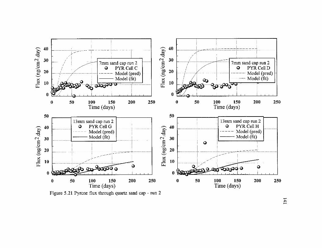
Flux

(ng/

cm2.

day)

Flux

(ng/

cm2.

day) 40

30 7mm sand cap run 2 © PYR Cell C

Model (pred) Model (fit)

20

10 n r

o

250100 150 2000 50Time (days)

9 40cd

rT 3 0ao

I p 2 0

X3E

10

5013 mm sand cap run 2

O PYR Cell G Model (pred) Model (fit)30

20

10

0 O0

200 250100 1500 50

50

s ; 40cdnd

rT 3 06o

20

xrB 10Ph

o

Time (days)Figure 5.21 Pyrene flux through quartz sand cap - run 2

7mm sand cap run 2 © PYR Cell D

Model (pred) Model (fit)

50

p a w

100 150Time (days)

200 250

13mm sa © I

nd cap run 2 >YR Cell H vlodel (pred) vlodel (fit)

--------- j--------- 1

Q

JSk

....

i i i..i.i....> ©

, , , ,3

i i i i

50 100 150 200 250Time (days)

&T50T3cT 1 100

50Ph

0

0

<P

50

i l o .

7mm sand cap Q DBF CeU C

Model (pred) Model (fit)

100 150Time (days)

200 250

ce 80

%

13mm sand cap O DBF Cell G

Model (pred) Model (fit)

50 100 150Time (days)

200 250

Figure 5.22 Dibenzofuran flux through quartz sand cap

7mm sand cap O DBF Cell D

Model (pred) Model (fit)

100 150Time (days)

200 250

«s 80

913mm sand cap

O DBF CeU H Model (pred) Model (fit)

0 50 10.0 , 150Time (days)

200 250

4

^ 200

3mm Pon cap© DBF CeU A

Model (pred) Model (fit)

300

100 150Time (days)

250

300

©y 200

TO

3mm Pon cap © DBF CeU I

Model (pred) Model (fit)

100 150Time (days)

250

200

3mm Pon cap © DBF CeU B

Model (pred) Model (fit)

E 50

100 150Time (days)

Time (days)

250

“ 200

©

3mm Pon cap © DBF CeU J

Model (pred) Model (fit)

250

Figure 5.23 Dibenzofuran flux through Pontchartrain cap

& 75T3cT

£o 5013)fl,

¥ 25

100

50

7mm sand cap Q PHE CeU C

M0del (pred) Model (fit)

O

150 100 150

Time (days)200 250

13mm sand cap @ PHE CeU G

Model (pred) Model (fit)

100 150Time (days)

200 250

Figure 5.24 Phenanthrene flux through quartz sand

Flux

(ng/

cm^.

flay

) Flu

x (ng

/cm

2. da

y)

- 7mm sand c. O PHI

Mo

ipi C eUD lei (pred) iel (fit)" I- /1~ I

Mo

jl

Orv% QGi ®

fj. . . . ' ’ i- ‘_ , , , ,

0 50 100 150 200 250Time (days)

100

13mm sand cap O PHE CeU H

Model (pred) Model (fit)

50

0 50 100 t 150 Tune (days)

200 250

►—* 4 4

>>1003mm Pon cap

© PHE Cell A Model (pred) Model (fit)

c n 80

Q-^03 q Qq

20

0 50 10.0 , , 150Time (days)

200 250

120

>>100

cn 803mm Pon cap

© PHE Cell I Model (pred)

Model (fit)

u, 20

50 100 150Time (days)

200 250

Figure 5.25 Phenanthrene flux through Pontchartrain cap

3mm Pon cap© PHE Cell B

Model (pred) Model (fit)

>>100

c n 80

0 50 100 150 200Time (days)

250

120

>>100C$c n ' 80

B^ 60E" 40

E 20

0

- 3mm Pon cap © PHE CeU J

Model (pred) Model (fit)

’a .... ............-.............1

c\.............1...............

' ^\

*©----- © V(w ! Q

91 ....

Q f - □//civS'/ICjkl i

QBi" i i i ___1_1_1_!_;_1_1_1_ i , , , , i , , ,

0 50 100 , 150 200Tune (days)

250

42*Ui

146

the uncapped flux would eventually fall below that of the capped system, and the result

of capping would be the exchange of high level acute exposure risk for low level

chronic exposure. However, as discussed in §2.1.4 long term degradation of most

compounds is likely, particularly given the potential for centuries long containment

afforded by field thickness caps (on the order of 1 meter). The effect of degradation

is discussed in Chapter 6 and a mathematical treatment is presented in Appendix D.

The effect of cap thickness and partition coefficient was also demonstrated in the

data. For example, in Figure 5.21, Figure 5.22, and Figure 5.24, the quasi-steady

(post-maximum) flux for dibenzofuran, phenanthrene, and pyrene through 7 and 13 mm

sand caps can be compared. For each chemical and for duplicate CSCs, the quasi­

steady flux is approximately 1.7 times larger through the thinner cap. This is

approximately the ratio of cap thicknesses (1.85) as one would expect in a diffusion

controlled system at steady state. Compare the quasi-steady phenanthrene flux of

approximately 35 ng • cm'2 • day'1 through the 7 mm sand cap to the 60 ng • cm'2 • day'1

flux through the 3.4 mm Pontchartrain cap. The ratio of fluxes is 1.7 and the ratio of

cap depths is 2.1, again demonstrating the effect of path length on the release rate.

This comparison also demonstrates that the cap organic carbon content (and thus the

partition coefficient), in the absence of degradation, has only a small effect on the

quasi-steady release rate through a cap. This is an anticipated result since under the

quasi-steady condition described, no transient accumulation would occur, and the

diffusion would not be retarded by sorption to the stationary sediment, leaving as the

primary resistance to mass transfer the path length.

147

Cap thickness will also affect the breakthrough time. This effect is most clearly

demonstrated in Figure 5.24. Comparing the 7 and 13 mm sand cap data, the time

required to reach the maximum flux was 7 and 13'A days respectively. Although not

strictly a breakthrough time, the time-to-maximum-flux is easier to quantify (and

visualize) in these systems and is directly proportional to the breakthrough time defined

by the first non-zero flux measurement. This is because for a particular system the

significant factors affecting the release rate do not change between breakthrough and

the maximum flux. The time ratio is nearly the same as the cap thickness ratio in this

case; however, this is not generally the case as shown in §4.1.6

In the absence of degradation, the primary effect of increasing the cap layer

partition coefficient is to increase both the breakthrough time and the time-to-maximum-

flux and to decrease the maximum flux. It is obvious why the time-to-maximum-flux

increases with the partition coefficient: it simply takes longer to fill the available

sorption sites in the cap. It is perhaps less obvious why the maximum value should

decrease as well. If the cap were to be thought of as a film with a certain resistance

to mass transfer (in the quasi-steady state), then a cap which saturates more rapidly will

have a larger concentration difference across it (i.e. less depletion of the lower layer)

and thus a larger flux through it than one which has a high sorption capacity. Of

course, for the case discussed in §4.1.4 where the concentration of the contaminant

remains constant in the contaminated layer because the loading exceeds the critical

loading, the maximum flux will not be affected by the cap layer partition coefficient.

148

The experimental design confounds the effect of cap thickness with that of

partition coefficient because there was not a treatment in which the same cap thickness

for two different sediments (with different partition coefficients) was used, therefore the

effect of lowered maximum flux due to the effect of larger cap layer partition

coefficient is not immediately obvious in the data. However, the effect of increasing

time-to-maximum-flux was demonstrated. Consider Figure 5.24 and Figure 5.25, for

the 7 mm sand cap the maximum dibenzofuran flux was reached in less than 10 days

while for the 3 mm Pontchartrain cap the maximum flux was not reached until nearly

40 days. This observed difference must be due to the deference in partition coefficient

since the difference in cap thickness for these two cells would have resulted in faster

breakthrough for the Pontchartrain cap.

§5.4.2.2 Sediment concentration profiles. After the second cap run the sediment

in the CSCs was cored and sectioned. The 2 mm sections obtained were extracted using

the column extraction technique developed and presented as Appendix C. The sediment

phase tracer concentration profiles obtained are presented below. As for the uncapped

profiles, the data from each experimental treatment have been pooled for each chemical.

The sediment tracer loadings reported have been corrected for water content of the

sediment sample extracted and are presented in units of ng analyte/g dry sediment

(ppm). The modeled profiles presented in Figure 5.26 to Figure 5.34 are discussed in

Chapter 6. It should be again noted that the ’fitted’ profiles were not fit to the profile

data, but were calculated using parameter values obtained from fitting the flux versus

time data presented in §5.4. As before the vertical lines shown on the profiles

149

represent the range of observed sediment loading for that particular section, and the

number printed in the center column is the number of replicate measurements for that

section.

§5.4.2.3 Capped profiles. The profiles clearly show the effect of the cap in

containing the contaminants. A large change in the sediment load is apparent at the cap

layer-contaminated layer interface. This is particularly noticeable with the sand cap, and

it is primarily due to the large difference in the partition coefficient for the tracers

between the two layers. Low extraction efficiency is probably the reason for the

observed difference between the model and experimental profiles for pyrene. The mass

balance calculations for these profiles were discussed in §5.4.1.2, 5.4.2.2.

The results presented in the previous sections provide experimental data against

which theoretical models of the dynamics of contaminant release can be compared. In

addition the potential of capping as a remediation option for the isolation of

contaminated sediments from the aquatic ecosystem is clearly demonstrated in both the

reduction of the contaminant release rate from the sediment after capping and the

containment evident in the contaminant profiles.

Sedi

men

t loa

d (p

g/g)

3 mm Pontchartrain Cap - DBF Model (fit)Observed Model (pred)

10-12 12-14 14-20

Depth (mm)

Figure 5.26 Sediment concentration profile for dibenzofiiran - Pontchartrain cap. The vertical line denotesthe experimental range. The number of replicate sections analyzed is given for each depth range.

Sedi

men

t loa

d (p

,g/g

)400

350

300

250

200

150

100

50

0

Figure 5.27 Sediment concentration profile for phenanthrene - Pontchartrain cap. The vertical linedenotes the experimental range. The number of replicate sections analyzed is given for each depth range.

3 mm Pontchartrain Cap - PHE

6-8

Depth (mm)8-10 ' 10-12 ' 12-14 ' 14-20

Sedi

men

t loa

d (j

ig/g

)1,400

3 mm Pontchartrain Cap - PYR Model (fit)Observed Model (pred)

6-8

Depth (mm)8-10 ' 10-12 ' 12-16 ' 16-20

Figure 5.28 Sediment concentration profile for pyrene - Pontchartrain cap. The vertical line denotes theexperimental range. The number of replicate sections analyzed is given for each depth range.

Sedi

men

t loa

d (p

g/g)

300

250

200

150

100

50

0

Figure 5.29 Sediment concentration profile for dibenzofuran - 7 mm sand cap. The vertical line denotesthe experimental range. The number of replicate sections analyzed is given for each depth range.

7 mm Sand Cap - DBF Model (fit) Observed Model (pred)

4

6-8 8-10

Depth (mm)10-12 12-16 16-20

Sedi

men

t loa

d (j

ig/g

)400

350

300

250

200

150

100

50

0

Figure 5.30 Sediment concentration profile for phenanthrene - 7 mm sand cap. The vertical line denotesthe experimental range. The number of replicate sections analyzed is given for each depth range.

7 mm Sand Cap - PHE Model (fit)Average Model (pred)

4

12-16 16-20

Depth (mm)

Sedi

men

t loa

d (p

g/g)

1.4007 mm Sand Cap -PYR

Model (fit) Observed Model (pred)

4

6-8 8-10 10-12 12-16 16-20

Depth (mm)

Figure 5.31 Sediment concentration profile for pyrene - 7 mm sand cap. The vertical line denotes theexperimental range. The number of replicate sections analyzed is given for each depth range.

Sedi

men

t Lo

ad (|J

,g/g

)300

250

200

150

100

50

0

Figure 5.32 Sediment concentration profile for dibenzofuran - 13 mm sand cap. The vertical line denotesthe experimental range. The number of replicate sections analyzed is given for each depth range.

Depth (mm)

Sedi

men

t loa

d (ja

g/g)

400mm Sand Cap - PHE Model (fit)Observed Model (pred)

350

300

250

200

150

100

0-2 2-4 4-6 6-8 8-10 10-12 12-14 14-16 16-18 18-22 22-26

Depth (mm)

Figure 5.33 Sediment concentration profile for phenanthrene - 13 mm sand cap. The vertical line denotesthe experimental range. The number of replicate sections analyzed is given for each depth range.

1,400

1,200

&D^ 1,000

'S 800

^ 600 &a:g 400

200

0

Figure 5.34 Sediment concentration profile for pyrene - 13 mm sand cap. The vertical line denotes theexperimental range. The number of replicate sections analyzed is given for each depth range.

13 mm Sand Cap - PYRModel (fit) Observed Model (pred)

1

4-6 6-8 8-10 10-12 12-14 14-16 16-18 18-22 22-26

Depth (mm)

Chapter 6 Model Evaluation

In this chapter I will compare the results of the three models developed in

Chapter 4 with the laboratory scale experimental results presented in the preceding

sections. A priori estimates or measured values for the model parameters were used for

calculating the predicted fluxes and profiles shown on the figures in this chapter. In

order to fit the model to the data certain parameters were adjusted. In the case of

uncapped flux only the water side mass transfer coefficient was adjusted, either directly

as in the case of the TCP data from Wang et al. (1991), or via adjustment of the

constant factor appearing in equation (4-4). In fitting the capped run data a maximum

of three parameters were adjusted: the water diffusivity and the cap and contaminated

layer partition coefficients. Of course in the case of pyrene, which was loaded above

the critical loading in both runs, the contaminated layer partition coefficient does not

appear in the model. These three parameters have significant roles in determining the

dynamics of the tracer release, and it was for this reason that they were chosen as the

adjustable parameters. The contaminated layer partition coefficient determines the total

tracer mass in the (model) system, the cap layer partition coefficient determines the

mass of tracer which can be held by the cap layer, and the diffusivity governs the rate

of mass transport.

The method of least squares was used to determine the best fit to the data. I

limited the range of variation in the partition coefficients to plus or minus 0.1 log unit

from the measured or published value of K()C. I limited the range of the diffusivity to

159

160

plus or minus 20% of the value predicted from the Wilke-Chang method. Deviations

from these guidelines are discussed individually in the following presentation.

Fluxes from uncapped CSCs were fit using a weighted residual. The minimum

sum of weighted residuals was used as the merit function in fitting these data. The

weighted residual was: where Y, is the observed flux at time t and y is the‘ t

V Y tmodel prediction at time t. This weighted residual was chosen because of the

exponential character of the dynamics. At short times the fluxes are high and the same

percentage difference between the observed and predicted gives a much larger

unweighted residual artificially increasing the influence of these data in the merit

function (i.e. sum of residuals squared). The result is that the initial few points are

quite close to the fitted model trace while data taken at longer times when the flux is

lower fall consistently and significantly below the model trace. The weighted residual

distributes the influence of the data more evenly in this case resulting in a more even

fit of the data.

§6.1 Base case

The data from the uncapped control cells from the two experimental capping

runs were used to evaluate the base case model derived in §4.1.3. Both the release rate

and the sediment concentration profiles were compared to the model predictions.

§6.1.1 Contam inant flux. The base case model predictions are compared to

previously published experimental data in Figure 6.1 (Wang et al., 1991). Equation

(4-4) predicts a mass transfer coefficient between 2.0 and 2.8 cm/day depending on the

overlying water depth (0.5 to 0.3 cm). The best fit (minimum unweighted sum of

squared residuals) of the model to the data is for k, = 2.55 cm/day. Note that the fit

is reasonable even without including water-side resistances which, for a moderately

soluble compound like TCP, should be expected as explained earlier (§4.1.1.1).

Figure 5.14 presented the dibenzofuran and phenanthrene fluxes for the

uncapped control cells in the second cap run. In this case equation (4-4) was used to

predict a mass transfer coefficient for the model, and the data was fit by adjusting the

constant factor in that relationship. A more precise fit to the data is possible if

additional model parameters were to be adjusted; however, I felt that the agreement

2.0e5

1.5e5 Uncapped TCP flux O Observed

kl = inf kl = 2.55 sq cm/day

C 4*

Sw1.0e5exa

15 20 25 30 35100 5Time (days)

Figure 6.1 Comparison of observed and predicted TCP flux from an uncapped CSC

162

using a single adjustable parameter was acceptable. Table 6.1 and Table 6.2 present

the fitted parameter values used in the model of the data presented in Figure 5.14. The

mass transfer coefficient found by fitting the base case model to the dibenzofuran and

phenanthrene data was 0.5 and 0.72 respectively, these values are 2-4 times larger than

the estimate made from the pyrene data in §5.4.1.1. It seems likely that the inaccuracy

of the water depth measurement again is responsible for the discrepancy in the

estimates.

§6.1.2 Sediment profiles. Post mortem sediment loads for the three tracers used

in the second capping run were presented in §5.4.1.2, 5.4.2.2. The a priori predictions

as well as the fitted predictions based on the results of the contaminant flux parameter

fits are presented. The primary difference between the a priori and fitted model

Table 6.1 Comparison of predicted and fit model parameters for cap run 2

DIBENZOFURAN

Parameter

Treatment, T Quartz sand No capr cap

Pontchartraincap

Mass transfer Predicted 1.165 — —

coefficient factor Fit 0.5 — —

Water diffusivity Predicted 0.516 0.516 0.516cm2/day Fit 0.516 0.31 0.45Cap layer Kd Predicted — 4 63L/kg Fit — 1.4 40Contaminated layer Kj Predicted 324 324 324L/kg Fit 324 290 260Residual sum of Predicted 3.86 417600 1120000squares Fit 2.25 28440 138000

163

Table 6.2 Comparison of predicted and fit model parameters for cap run 2

PHENANTHRENE

Parameter

Treatment

No cap Quartz sand cap

Pontchartraincap

Mass transfer Predicted 1.165 ------------ -----------

coefficient factor Fit 0.72 ------------ -----------

Water diffusivity Predicted 0.5 0.5 0.5cm2/day Fit 0.5 0.26 0.30Cap layer Kd Predicted — 12 220L/kg Fit — 1.6 45Contaminated layer Kd Predicted 1110 1110 1110L/kg Fit 1110 880 820Residual sum of Predicted 3.99 89700 98430squares Fit 3.08 2270 12820

concentration profiles is the difference in the contaminated layer partition coefficient.

Because the models only predict the pore water concentration, the sediment load was

inferred through the partition coefficient, thus differences in partition coefficient lead

directly to differences in the sediment phase concentration profile. The predicted values

were calculated by numerical integration of the model over the appropriate interval.

Simpson’s method was used for the integration (Press et al. , 1992). The computer code

is presented as Appendix D. The model concentration profiles are reasonably close to

the observed concentration profiles; most of the predictions fall within the range of the

experimental observations as indicated by the vertical line in the plots.

164

§6.2 One-layer model

The one layer model was used to examine the dynamics of pyrene in these

systems as described in §5.4. For both of the cap runs described in §3.1.7, the pyrene

loading on the sediment was above the critical loading, which, based on the data in

Table 3.2, is 782 mg/kg. Thus for these data, the appropriate model is one in which

the concentration at the bottom of the cap layer remains constant. Table 6.3 presents

the parameters used in and fit by the model.

§6.2.1 Contam inant flux. For the Pontchartrain cap (Figure 5.18 and Figure 5.19)

the a priori model results are in reasonable agreement with the observed fluxes. The

breakthrough time is quite accurately predicted although the magnitude of the flux is

over predicted. It is clear that the quasi-steady state expected at long times in this

system had not been reached and thus evaluation of the model remains incomplete.

Nevertheless in this case the quantitative predictions are within a factor of 2 of the

Table 6.3 Comparison of predicted and fit model parameters for cap run 2

PYRENE

Parameter

TreatmentQuartz sand cap Run 1 Run 2

Pontchartrain cap Run 1 Run 2

Water diffusivity Predicted 0.478 0.478 0.478 0.478cm2/day Fit 0.38 0.38 0.38 0.38

Cap layer Kd Predicted 38 38 790 790L/kg Fit 70 60 820 900

Residual sum of Predicted 14030 54100 13080 10680squares Fit 3240 16300 1420 2050

165

observations, and this indicates that for the higher organic carbon content cap material,

the model incorporates the major mechanisms. The fit of model to the Pontchartrain

cap data is good which is an indication that the major factors influencing the dynamics

of pyrene release are incorporated in the model.

For the sand cap, (see Figure 5.21) the rapid breakthrough and essentially

constant flux does not appear to be consistent with the model. The lower (than

predicted) steady-state flux and rapid breakthrough observed in this case are consistent

with a thicker cap having a lower partition coefficient than that measured for pyrene

(or a lower than estimated diffusivity). Another possible explanation for the rapid

breakthrough is that the cap was fractured and preferential paths for the diffusion of the

tracers existed; however, I did not observe any large deformations of the caps. In

addition, preferential paths through the cap should tend to decrease the mass transfer

resistance of the cap and presumably lead to increased flux over the model prediction -

the opposite of what was observed. The over prediction of the modeled fluxes is,

however, consistent with evaporative losses from the system. This is because the

effluent aqueous concentration was used to infer the experimental fluxes and evaporative

losses would decrease this measured value leading to artificially low experimental

fluxes. The over prediction of the model in this case is also conceivably due to

depletion in the contaminated layer, which would reduce the observed release rate, but

is not accounted for in the model since this would require modeling the transition across

the critical sediment loading concentration. Another factor which probably contributes

to the observed over prediction of the release rates is that water-side mass transfer

166

resistance was not incorporated in the cap models. A simple calculation comparing the

cap resistance at steady state given by a jD wz4/3 with the water side resistance given

by l / k w indicates that for pyrene between 10 and 30 percent of the overall mass transfer

resistance is associated with the water side. Thus experimentally an additional

resistance was present which would tend to depress the release rate and contribute to

the model over prediction.

§6.2.2 Sediment profiles. The pyrene profile for the second run shows

considerably greater depletion than expected based on the mass lost to the overlying

water as calculated from the measured release rate. It is seems likely that poor

analytical recoveries from the sediment are the source of this discrepancy as discussed

in §5.4.1.2. The concentration profile data were not used in fitting the model; the

modeled concentration profiles are presented for comparison only.

§6.3 Two-layer model

The data collected for dibenzofuran and phenanthrene in the second cap run was

used to evaluate the two-layer model. These chemicals were loaded onto the sediment

at 10% and 80% of their respective critical loading, and depletion of the chemicals

from the inoculated layer was expected to be significant.

§6.3.1 Contam inant flux. Figure 6.2 presents a comparison of the model results

to previously published experimental data and Table 6.4 presents the physico-chemical

parameters used in the model (Wang et a l., 1991). The solid line is the predicted flux

based on measured or estimated parameter values. The dotted line was fit to the data

167

Table 6.4 Experimental and fit parameters for TCP data.

Inoculation Batch IBalsam Sand Cap Tao River Cap

Predicted Fit Predicted FitDw (cm2/day) 0.62 0.85 0.62 0.72

cA

eiPj (g/cm3)

0.381.53

0.381.53

0.50.84

0.50.84

P KD1 (cm3/g) 0.98 0.98 4.6 4.6Cap depth (cm) 0.7 0.7 0.7 0.7

e2 0.45 0.45 0.45 0.45C p2 (g/cm3) 0.81 0.81 0.81 0.81oN Kd2 (cm3/g) 27.5 23.5 27.5 30

TA

Contaminated depth (cm)

1.5 1.5 1.5 1.5

M Initial [TCP] (mg/L)

150 150 150 150

Inocu ation Batch IIQuartz Sand Cap University Lake Cap

Predicted Fit Predicted | Fit

Dw (cm2/day) 0.62 0.82 0.62 1.21

C ei 0.37 0.37 0.45 0.45A p, (g/cm3) 1.61 1.61 0.81 0.81P KD1 (cm3/g) 1.79 1.79 27.5 113

Cap depth (cm) 0.6 0.6 0.7 0.7

€2 0.45 0.45 0.45 0.45C p2 (g/cm3) 0.81 0.81 0.81 0.81ON

Kd2 (cm3/g) 27.5 120 27.5 113

TA

Contaminated depth (cm) 1.5 1.5 1.5 1.5

M Initial [TCP] (mg/L) 250 250 250 250

Flux

(mg/

cm2.

day)

Flux

(mg/

cm

day) 60

<n ' 50I 4 0

a 30

30

20© Quartz sand cap Model (pred) Model (fit)

© Balsam sand cap Model (pred) Model(fit)

10^ 10

0

0 5 10 15 20 25 30 35 4020 2515100 5Time (days) Time (days)

50

30

20Balsam sand cap Model (pred) Model(fit)

10

0

20 2510 150 5

UL cap Model (pred) Model (fit)

0 10Time (days)

Figure 6.2 Comparison of observed and predicted TCP flux from capped CSCs.

15 20 25Time (days)

30 35 40

ON00

169

using only the water diffusivity and contaminated sediment partition coefficient as

adjustable parameters. The parameter values used in the model curves shown in

Figure 6.2 are presented in Table 6.4. In the experiments, the sediment used as the

contaminated sediment layer in all four runs was University lake sediment. However,

it was inoculated on two separate occasions, once for the Balsam and Tao cap runs and

later for the sand and University lake cap runs. Note from Table 6.4 that the fitted

contaminated layer partition coefficient is different for each inoculation batch. This

parameter was the most important in fitting the data, and the difference suggests some

change in sediment treatment or inoculation conditions. Literature correlations, based

on mostly pesticides and polyaromatic hydrocarbons, suggest that the partition

coefficient should fall between 2 and 70 L/kg (Lyman et al., 1990). The model

predictions are qualitatively correct, predicting both the form of the flux versus time

relation and the characteristic time to reach the maximum flux.

The data presented in §5.4 for the flux of dibenzofuran and phenanthrene

through Pontchartrain and quartz sand caps was also modeled. The parameter values

used in the model are presented in Table 6.1 and Table 6.2. In general the model

oveipredicts the observed flux. The magnitude of the over prediction is generally less

than a factor of 2. The breakthrough and approach to a maximum flux followed by slow

tailing off of the release rate are qualitatively demonstrated in the model predictions.

These observations support the modeling assumptions of sorption-retarded diffusion in

a porous medium on which these models are based.

170

§6.3.2 Sediment profiles. The concentration profiles predicted by the model (see

Figure 5.26 through Figure 5.34) are also in reasonable agreement with the observed

profiles. The general agreement with the model again supports the model assumptions

regarding the chemical dynamics in diffusive systems.

§6.4 DOC model

The simple model constructed by assuming constant physico-chemical properties

for the DOC (see §4.2) qualitatively describes the DOC release dynamics from the

laboratory simulators used in this work (Figure 5.4). Because a priori estimates of the

DOC diffusivity are not readily available, the model was used as tool to estimate the

diffusivity of the DOC used in this work. This was done by fitting the model to the

data by the method of least squares using the diffusivity as an adjustable model

parameter.

§6.4.1 Flow through cells. The three experimental runs, shown in Figure 5.4, for

Bayou Manchac were taken as a single dataset, and the model was fit to the data by

minimizing the sum (over all three runs) of the squared residuals using a single

adjustable model parameter, the water diffusivity of the DOC. All other parameters

were measured, including the partition coefficient for the DOC between the aqueous

and stationary sediment phases. The University Lake dataset was fit also fit by using

residual sum of squares as the merit function. For the UL dataset the value of the

partition coefficient (2.5 L/kg) reported by Koulermos (1989) was used although the

sediment samples were collected at different times. The fact that a single adjustable

171

parameter provides such a good quantitative description of the observed fluxes indicates

that, for the simple systems used in this study, the assumption of constant physico­

chemical properties for the DOC is reasonable. The fitted diffusivities, shown in

Table 6.5, extracted from the data agree well with previously presented values

(Koulermos, 1989). The values of the diffusivities are specific to the sediments chosen;

however, the conclusions derived from this work should be generally applicable to other

sediments as well.

§6.4.2 Beaker profiles. As shown in Figure 5.5, the modeled concentration profiles

match the experimental profiles quite reasonably. Table 6.6 presents the fitted effective

DOC diffusivities for the sediments used in the beaker experiments. These diffusivities

are of the same order of magnitude as effective diffusivities reported by Koulermos

(1989). This work demonstrates that natural DOC from a variety of sources are mobile

in a diffusion controlled regime. Additionally, for the sediments studied, the magnitude

of the effective diffusivities found are comparable, indicating that the simple approach

Table 6.5 DOC diffusivities fitted from flow cell experiments

SedimentWater Diffusivity

cm2 • d ay 1Effective Diffusivity

cm2 • d ay 1

Manchac 0.012 0.0012

University 0.09 0.032lake

172

Table 6.6 DOC diffusivities extracted from in-beaker profiles

ParameterUniversity

lakeLake

PontchartrainBayou

ManchacCocodrie

Initial [DOC]a (mg/L) 450 270 700 770

Effective diffusivity cm2/day (fit) 0.071 0.078 0.095 0.09

a Taken as the maximum observed value in the profile, except for Cocodrie where it was taken as an adjustable parameter.

to modeling DOC transport may be applicable over a range of conditions using a single

estimate for the DOC diffusivity. In addition, a relatively simple model for DOC

mediated contaminant transport should be applicable. Such a model was developed in

the §4.3.

§6.5 DOC enhanced transport model

Diffusion dominated chemical release from a semi-infinite sediment bed is the

situation considered by Thoma et al. (1991) in deriving the following relation for an

colloid enhancement factor

E = t j ( D e + D c C c K c ) / D e «-28)

This model of enhanced flux does not account for the transience of the DOC

flux observed in the laboratory systems studied. The expected behavior in these

systems is that the enhancement would decrease with time as the DOC flux falls.

However, if DOC are continuously released from the sediment as the data in §5.2.2.2

173

suggest, the DOC flux may reach a quasi-steady value in which case equation (4-27)

would be the appropriate starting point for the consideration of colloid mediated

contaminant transport. Nevertheless, it seems reasonable to estimate the initial

enhancement in the laboratory systems used here from the simple model.

Recall for these experiments two sediment treatments were used, one intended

to remove mobile colloids and a second intended to increase the quantity of available

mobile colloids. The treatments are denoted as the washed and frozen sediments

respectively. Based on equation (4-28) the expected enhancement of the frozen cells

over the washed cells at the beginning of the first run is small, ranging from 3% for

dibenzofuran to 35 % for pyrene for the first run. The above estimates were made using

22 mg/L DOC in the frozen cells, the fitted diffusivity of the DOC (§6.4.1), and

assuming that the partition coefficient to the DOC was equal to the organic carbon

normalized partition coefficient, Koc. No calculations were made for the data collected

in the second run because of the initially low level of DOC in the second run for the

frozen sediment; the expected enhancement for pyrene was 3% in the frozen cells -

within the experimental error for the measurements.

The clearest experimental evidence of enhanced flux due to the presence of

colloids is shown in Figure 5.10 for the phenanthrene data. Using the average of the

first three data points as an estimate of the initial tracer release rate yields a

phenanthrene flux of 336 ng • cm"2 • day'1 from the washed cells and 506 ng • cm"2 • day"1

from the frozen cells. The mathematical model predicting the unenhanced diffusive

chemical release rate is linear (equation (4-10)) in the initial concentration of the tracer,

174

thus one would expect that the flux from the frozen treatment to be larger in the ratio

of the initial chemical concentrations: 130 ju,g/L / 104 /xg/L = 1.25 times greater or

420 ng • cnr2 • day'1. The colloid enhancement for phenanthrene, given the specific

conditions of this run, should be about 10% during the initial period of the run, so a

rough estimate of the phenanthrene flux from the frozen cells (based solely on the data

from the washed cells) would be 1.1 -420 = 462 ng-cm"2-day'!. This is within 10%

of the observed average phenanthrene flux of 506 ng*cm'2-day_1. If the actual DOC

diffusivity or partition coefficient for phenanthrene to the DOC were only slightly larger

than the values used to make the estimate (from Table 3.6), the predicted flux would

be quite close indeed. A similar analysis of the pyrene data from run 1 (Figure 5.11)

gives the following: Initial average flux for the washed cells of 62 ng • cm'2 • day'1; and

for the frozen cells, 100 ng • cm'2 • d ay 1. The expected frozen cell flux without colloidal

enhancement would be 27/24.3 • 62 = 69 ng • cm"2 • day'1. If colloids enhanced the flux

by 35%, the frozen cell pyrene flux should be 93 ng • cm"2 • d ay 1. This is quite close

to the observed average flux from the frozen cells. These calculations are based on the

assumption that the physico-chemical properties of both the frozen and washed

sediments are identical. As can be seen from Table 3.1, this is not an unreasonable

assumption. Although these calculations seem to explain the difference between the two

treatments they do not prove that the mobile DOC were the source of the observed

difference in the initial flux. Further experiments using a range of higher DOC initial

concentrations should be performed to validate this estimate of the enhancement of

175

chemical flux. As discussed in §5.2.2.2, relatively high levels of DOC can be obtained

in the laboratory under anaerobic conditions.

§6.6 Summary

Mathematical models of physical systems must be validated by comparison to

experimental measurements. In chapter 4 1 presented several models which describe the

dynamics of colloid and contaminant release from sediment systems. I presented the

results, obtained from lab scale physical models of natural sediment systems, of the

release dynamics of colloids and contaminants in chapter 5. In this chapter the model

predictions have been assessed against the experimental data.

The models generally predict the dynamics of the systems studied quite well.

In the case of the uncapped release of hydrophobic chemicals from sediments, the a

priori model predictions based on measured or estimated parameters matched both

quantitatively and qualitatively the experimental data. In the case of the one-layer

model, valid for the case of a sediment loading above the critical loading, the data were

not collected for a long enough period to achieve steady state, and thus the evaluation

of this model remains incomplete. For the two-layer model, which incorporates the

depletion of the contaminant from the lower, inoculated sediment, the a priori model

estimates of the release rates consistently over predicted the observed fluxes of the

polyaromatic hydrocarbons. However, for the data presented by Wang et al. (1991),

the model consistently under predicted the observed fluxes.

176

The model describing the release of DOC from sediments provides a reasonable

estimate of the DOC diffusivity via least squares fit of the model to the observed DOC

flux from the laboratory simulator. The estimated diffusivities are based on the

assumption that the physico-chemical properties of the DOC are constant over all of the

size classes of the DOC. This simplification of the DOC properties seems to be

justified in the laboratory experiments performed since the DOC release dynamics are

accurately described by the model.

A simple predictor of the effect of DOC on the release rate of hydrophobic

chemicals (equation (4-28)), was validated by the experimental data collected. This

small dataset is insufficient to give complete confidence in the enhancement factor, but

does provide an experimental protocol by which to begin a systematic evaluation of the

colloid enhanced transport in sediments.

Chapter 7 Conclusions and Recommendations

§7.1 Conclusions

§7.1.1 DOC mobility. Experiments demonstrating the mobility of natural organic

colloids were performed. In simulators similar to the capping cells, DOC concentrations

measured in the effluent indicated that dissolved organic carbon was released to the

overlying water. In addition, pore-water DOC concentration profiles were obtained for

sediments taken from several different environments by periodic replacement of the

overlying water in a one-liter beaker filled with a sediment bed. The development of

these profiles from an initially homogeneous sediments showed that DOC from a variety

of sources are mobile in a diffusion controlled regime.

Under the controlled conditions of the laboratory, the dynamics of the release

of naturally occurring organic colloids from uncapped sediment was shown to closely

parallel the release of hydrophobic chemicals by exhibiting a rapidly decreasing flux to

the overlying water as a function of time. The mathematical models used to describe

hydrophobic organic chemical release dynamics also described the dynamics of the

DOC release. A simple model, in which the physico-chemical properties of the DOC

were assumed to be single-valued and invariant, was successfully fit to pore-water DOC

profiles from several sediments, from a freshwater stream and lake to brackish lake and

estuarine sediment. The diffusivity was used as the fitting parameter and the best fit

177

178

value was taken as the DOC diffusivity for that sediment. The diffusivity estimates

obtained in this fashion were in close agreement with the available literature values.

§7.1.2 Colloid facilitated transport. Experiments using sediment specially treated

to, on the one hand, increase the amount of mobile DOC, and, on the other hand, to

remove as much mobile DOC as possible, demonstrated the effect of DOC on

contaminant release rates to the overlying water from an uncapped sediment. The

chemical flux from the sediment with larger initial DOC concentration was greater than

the flux from the sediment with lower DOC concentration.

Two modeling approaches for colloid enhanced transport were discussed. One

based on an enhanced effective diffusion coefficient (previously published), and a

second which considered the DOC effect on chemical transport to be advective in

nature. The simpler (enhanced diffusivity) was compared to the experimental data from

one run and was found to predict the observed flux differences between experimental

treatments to within 10%. This result is encouraging, however it does not completely

validate the model. Suggestions for future work are made in the following section.

§7.1.3 Capping. Experimental verification of the effectiveness of capping as a

means of isolating contaminated sediment from the aquatic ecosystem was presented.

For the chemicals studied, polyaromatic hydrocarbons, even a cap as thin as 1 cm

resulted in an order of magnitude decrease in the hydrophobic organic chemical release

rate after 50 days compared to the release rate from an uncapped sediment. Greater

relative flux reductions were observed earlier in the run, while at longer times, lower

relative reductions in the flux were observed due to the continued decrease in the flux

179

from the uncapped sediment caused by the depletion of the contaminant load. The

chemical containment effect of cap was also apparent in sediment core profiles taken

after 200 days from the flow-through simulators of capped contaminated sediment. A

marked decrease in contaminant loading was observed in the cap layer compared to the

levels in the contaminated layer. Mass balance calculations also showed that the

fraction of the initial mass of contaminant lost to the overlying water was significantly

reduced by the presence of a cap.

The basis for a criterion indicating the importance of water-side mass transfer

resistances was developed. In field applications water-side resistances to mass transfer

are likely to be relatively unimportant. The exception to this is the estimation of the

base-case flux for highly hydrophobic chemicals (particularly when loaded above the

critical loading), when benthic water-side resistances should be the only important

factor affecting the chemical release to the overlying water. In laboratory analysis of

capped systems the water-side resistances may be important since the actual cap

thicknesses normally used are small compared to field placements, and the water flow

rates are also typically much lower than in the field. This may partially explain the

reason that the two-layer model over predicts the observed flux since there may have

been an additional experimental mass transfer resistance not accounted for by the cap

models. Development of lab scale tests for the effectiveness of proposed cap materials

should account for water-side effects because water-side resistance in the lab will

artificially enhance the apparent effectiveness of a cap material when compared to field

placement where water-side resistance is probably negligible.

180

Mathematical models describing the dynamics of hydrophobic organic chemical

release from sediment beds were developed, as were models for the release of

hydrophobic organic chemicals through a clean sediment cap placed upon the

contaminated sediment as a means of isolating the contaminants from the ecosystem.

The models generally give good qualitative and quantitative predictions for the chemical

release rate. The base case model correctly predicts the rapid decrease in the release

rate, while the two-layer model predicts the increase in flux through a maximum and

the following slow decline in release rate. The a priori quantitative predictions of the

models are within a factor of at most 4, and for several data sets within a factor of 2

or less of the observed chemical release rates. In conjunction with the good qualitative

description of the release rate dynamics, the match between the modeled and measured

in-bed concentration profiles supports the contention that the major transport pathways

are accounted for in the models of the laboratory system. These models provide the

first theoretical basis for the rational design of a cap as a chemical barrier. Due to the

long-term isolation in an anaerobic environment predicted by the models, the

degradation of even ‘refractory’ chemicals may occur, thus further enhancing the

effectiveness of a cap. Although not presented in the main text, the incorporation of a

first order degradation reaction is presented in Appendix D.

§7.2 Recommendations

§7.2.1 Colloid enhanced transport - experimental. The enhancem en t o f

contaminant flux due to the presence of natural DOC should be verified through further

181

experiments with sediments treated to diminish/enhance the available mobile DOC.

Larger differences in the initial DOC concentration will allow this subtle effect to be

more confidently quantified. The observation that DOC are released from the sediment

to the pore-water in laboratory systems provides a technique to provide high

concentrations of DOC in the sediment pore-water. This will allow testing the colloid

enhancement model at various levels of DOC in the sediment. This is an important

aspect of the experimental design used to ascertain the power of the model in explaining

the observed variability in the contaminant flux from differently treated cells.

§7.2.2 Colloid enhanced transport - modeling. In natural systems there is a

constant cycling of carbon. The diagenesis of detrital material results in the continual

production of DOC within the sediment bed. It is likely that some quasi-steady

production of DOC will result. Complete modeling of the effect of colloids on

contaminant transport should eventually include the dynamics of production and

Brownian diffusion of the colloids as well as the effects of sediment chemistry,

specifically the ionic strength and pH on the partitioning of contaminants to the

colloids. Changes in ionic strength and pH may cause conformational changes in the

colloids which in turn may affect the both the diffusivity and partition coefficient.

§7.2.3 Capping - experimental. Further work in the area of capping should

include investigation into the possible negative effects on the barrier performance of the

cap of random cap penetration by benthic organisms. For example deep burrowing

worms might breach even a thick cap and thus provide preferential pathways for the

release of the contaminants. Isolated scour or anchor placement might also cause a

182

local cap breach. The current understanding and models of the post cap dynamics of

contaminant release do not provide guidance in this area. Experiments using simulators

similar to those used in this study could be prepared with caps which were breached

(e.g. with a toothpick) to varying degrees to assess the effect of local cap failure on the

overall effectiveness of a cap.

As suggested in the literature review, the recolonization of the cap is affected

by the type of sediment used for the cap. Specifically, sandy caps attract suspension

feeders and silty caps attract burrowing (deposit) feeders. This suggests that composite

caps with a lower silty layer with relatively high organic carbon content covered by a

sand layer would provide an excellent chemical barrier by providing for sorption in the

lower layer while encouraging the recolonization of suspension feeders which will be

less likely to penetrate the cap. Experimental and modeling studies on the effectiveness

of composite caps of this nature should be performed.

Of the twenty-odd capping projects presented in the literature review, most have

used sand as the cap material due to the ease of placement. As this work clearly

shows, sand is not a particularly effective chemical barrier. Experiments aimed at

modification of the sand via amending with fly ash or an ionic surfactant via ion

exchange should be performed to determine whether engineered sand caps will provide

enhanced chemical containment while maintaining the advantageous placement

characteristics.

This work has focused on the release of hydrophobic organic chemicals. Many

contaminated sites exist with high levels of heavy metals. As mentioned in the

183

literature review, the sediment chemistry will play an important role in the transport of

metals due to their changing oxidation state as the local redox potential changes. The

changing oxidation state will change the metal solubility, which in turn will affect the

mobility of the ion. Metal migration in capped systems should be investigated both

experimentally and through models incorporating the changing sediment chemistry and

its effect on the metal mobility.

It is possible that sediments which have been contaminated for decades may have

different desorption properties than laboratory inoculated sediments. Specifically, the

desorption may be kinetically controlled by the intraparticle diffusion of the contaminant

molecule from the interior of a sediment particle to its surface where it enters the water

phase and ultimately diffuses to the overlying water. Experiments should be performed

which can assess this possibility. Contaminated sediment obtained from a (Superfund

or other) contaminated site should be used in conjunction with freshly inoculated (at

approximately the same level) sediment in parallel simulator cells to ascertain an effect

of sediment age. It might also be possible to inoculate a series of sediment subsamples

in the laboratory and store them for varying lengths of time before beginning an

experimental run.

§7.2.4 Capping - modeling. The agreement of the models with the experimental

capping data indicates that the transport mechanisms have been reasonably modeled.

These models thus provide a foundation upon which to construct more complex models

which will more closely match conditions likely to be found in the field. The models

which have been presented are primarily intended as tools for exploring the diffusive

184

transport mechanism operative in bed sediments and are not intended to be directly

applicable in the field. Many field conditions exist which were not incorporated.

These conditions include sediment heterogeneity (both physical properties and

contaminant distribution), biodegradation, erosion and deposition, non uniform initial

contamination (an existing pollutant profile), and diffusion into deeper sediment.

Further study of the advective transport of pollutants through sediment (which might

be induced by tidal variations, water table height variations, or salinity or thermal

gradients) is also needed so that this mechanism can be incorporated in future transport

models. In addition many sites exist in which the contaminant loading exceeds the

critical loading, this is necessarily only a temporary situation and the transition to

loadings below the critical loading should be considered.

More complex models will also be required for metals transport since the local

redox potential affects the mobility through its partitioning/solubility characteristics.

After the inclusion of metals transport, the models will provide a basis for the

evaluation of the pollutant source potential for contaminated sediment sites. Risk based

prioritization of the remediation of contaminated sediment sites will then be a realistic

goal.

Bibliography

Ariathurai, R., MacArthur, R. C., and Krone, R. B. (1977) Mathematical model of estuarine sediment transport, Technical Report D-77-12. US Army Engineer Waterways Experiment Station, Vicksburg, MS

Atwell, R. W ., and Colwell, R. R. (1981) Actinomycetes in New York Harbor sediments and dredging spoil, Marine Pollution Bulletin, 12, 351-353.

Averett, D .E ., Perry, T. and Miller J.A. (1990) Reviews of removal, containment and treatment technologies for remediation of contaminated sediment in the Great Lakes, Miscellaneous Paper EL-90-25, US Army Engineer Waterways Experiment Station, Vicksburg, MS

Baldwin, K. C., Irish, J. D ., and Bokuniewicz, H. J. (1990) "Real-time in-situ monitoring of dredge disposal sites," in Geotechnical Engineering of the Ocean. Vol. STP 1087 (pp. 76-86). ASTM: Philadelphia, PA.

Baron, J.A ., L.J. Thibodeaux, D.D. Reible, P.H. Templett, and C.B. Henry JR(1990). Laboratory simulation of diffusion in contaminated marine sediments, Estuaries, 13, 81-88.

Bauer, J.E ., and D.G. Capone (1988). Effects of co-occurring aromatic hydrocarbons on degradation of individual polycyclic aromatic hydrocarbons in marine sediment slurries, Appl. Environ. Microbiol., 54(7), 1649-1655.

Bird R.B., Stewart, W.E. and Lightfoot, E.N. (1960) Transport Phenomena. John Wiley & Sons, New York

Bokuniewicz, H ., and Gordon, R. (1980) Deposition of dredged sediment at open water sites, Estuarine and Coastal Marine Science, 10, 289-303.

Bokuniewicz, H ., Cerrato, R., and Hirschberg, D. (1986) Studies in the lower Bay of New York Harbor associated with the burial of dredged sediment in subaqueous borrow pits, State University of NY: Marine Sciences Research Center.

Bokuniewicz, H. J., Gebert, J., Gordon, R. B., Higgins, J. L., Kaminsky, P., Pilbeam, C. C ., Read, M ., and Tuttle, C. (1978) Field study of the mechanics of the placement of dredged material at open water disposal sites, DMRP Technical Report, D-78-7. US Army Engineer Waterways Experiment Station: Vicksburg, MS

185

186

Bokuniewicz, H. (1989) "Behavior of sand caps on subaqueous dredged-sediment disposal sites," In Scientific Monitoring Strategies for Ocean Waste Disposal: Ocean Processes in Marine Pollution. Vol. 4. 221-229. Kreiger Publishing.

Bokuniewicz, H ., Gebert, J., Gordon, R. B., Kaminsky, P ., Pilbean, C. C., Reed, M., and Tuttle, C. (1977) Field study of the effects of storms on the stability and fate of dredged material in subaqueous disposal areas, DMRP Technical Report, D-77-22. US Army Engineer Waterways Experiment Station: Vicksburg, MS

Boudreau, B.P. (1986). Mathematics of tracer mixing in sediments: II. Nonlocal mixing and biological conveyer-belt phenomena, American Journal o f Science, 286, 199-238.

Boyd, S., J. Lee, and M. Mortland (1988). Attenuating organic contaminant mobility by soil modification. Nature, 333, 345-347.

Brandes, H ., Silva, A., and Fredette, T. (1991) Settlement of offshore mounds of capped dredged materials, Maritimes, November, 12-14.

Brannon, J. M ., Plumb, R., and Smith, I. (1980) "Long-term release of heavy metals from sediments," In Contaminants and Sediments. R. Baker (Ed.), Vol. 2 (pp. 221-265). Ann Arbor Science Pub.: Ann Arbor, MI.

Brannon, J., and Poindexter-Rollins, M. E. (1990) Consolidation and contaminant migration in a capped dredged material deposit, Sci. Tot. Env., 91, 115-126.

Brannon, J., Sturgis, R. H. T., Smith, I., and Gunnison, D. (1986) Dredging operations technical support program effectiveness of capping in isolating Dutch Kills Sediment from Biota and Overlying Water, Miscellaneous Paper, D-86-2. US Army Engineer Waterways Experiment Station: Vicksburg, MS

Brannon, J. M ., Hoeppel, R. E., Sturgis, T. C., Smith, I., and Gunnison, D. (1985) Effectiveness of capping in isolating contaminated dredged material from biota and the overlying water, Technical Report, D-85-10. US Army Engineer Waterways Experiment Station: Vicksburg, MS

Brannon, J., Hoeppel, R., and Gunnison, D. (1987) Capping contaminated dredged material, Marine Poll. B u ll, 18, 175-179.

Broughton, J. D. (1977) Investigation of subaqueous borrow pits as potential sites for dredged material disposal, Technical Report D-77-5. US Army Engineer Waterways Experiment Station: Vicksburg, MS

187

Browman, M. G., and Chesters, G. (1977) "The solid-water interface: Transfer of organic pollutants across the solid-water interface," In I. H. Suffet (Ed.), Fate o f Pollutants in the Air and Water Environments, Part I (pp. 49-105).

Brown, J. F ., Jr., Bedard, D. L., Brennan, M. J., Carnahan, J. C., Feng, H ., and Wagner, R. E. (1987) Polychlorinated biphenyl dechlorination in aquatic sediments, Science, 236, 709-712.

Brown, J. F ., Wagner, R. E., Bedard, D. L., Brennan, M. J., Carnahan, J. C ., May, R. J., and Tofflemire, T. J. (1984) PCB transformations in Upper Hudson [River, USA] Sediments, Northeast. Environ. Sci., 3, 167-179.

Brownawell, B .J., and J.W. Farrington (1986). The biogeochemistry of PCBs in interstitial waters of a coastal marine sediment, Geochim. Cosmochim. Acta, 50, 157-169.

Brownawell, B.J., and J.W. Farrington (1985). Partitioning of PCBs in marine sediments, In Sigleo, A .C., and A. Hattori (Eds.), Marine andEstuarine Geochemistry, Vol. 7 (pp. 97-120). Lewis Publishers.

Bruin, J., Van Hattem, W. A., and Wijnen, E. J. E. (1985) "Delfshaven-Rotterdam, redevelopment of a contaminated area," In Contaminated Soil: Proceedings of the First International Conference on Contaminated Soil, P 913-915. Applied Scientific Research (TNO) and The Netherlands Ministry for Housing, Physical Planning and the Environment (VROM).

Burks, S. A., and Engler, R. M. (1978) Water quality impacts of aquatic dredged material disposal (Laboratory investigations). Technical Report, DS-78-4. US Army Engineer Waterways Experiment Station: Vicksburg, MS

Butt, A ., Alden, R., Hall, G., and Jackman, S. (1985) "Contained dredged material for open ocean disposal," In Proceedings of the Fourth Symposium Coastal and Ocean Management, Vol 1. 578-594. ASCE

Capel, P .D ., C. Leuenberger, and W. Giger (1991). Hydrophobic organic chemicals in urban fog, Atmospheric Environment, 25A, 1335-1346.

Cargill, K. W. (1985) Mathematical model of the consolidation/desiccation process in dredged material, Technical Report D-85-4, US Army Engineer Waterways Experiment Station: Vicksburg, MS

188

Caron, G., I.H. Suffet, and T. Belton (1985). Effect of dissolved organic carbon on the environmental distribution of nonpolar organic compounds, Chemosphere, 14, 993-1000.

Carslaw, H. S., and Jaeger, J. C. 11959) Conduction of Heat in Solids. Second Edition. Oxford University Press: Oxford, England.

Chiou, C .T., R.L. Malcolm, T.I. Brinton, and D.E. Kile (1986). Water solubility enhancement of some organic pollutants and pesticides by dissolved humic and fulvic acids, Environ. Sci. Technol., 20, 502-508.

Clausner, J. E., and Abel, C. E. (1987) Disposal alternatives for PCB-contaminated sediments from Indiana Harbor, Indiana; Vol II: Appendix J, Miscellaneous Paper, EL-87-9. US Army Engineer Waterways Experiment Station: Vicksburg, MS.

Cline, J. T., and Upchurch, S. B. (1973) "Mode of heavy metal migration in the upper strata of lake sediment," In Proceedings of the 16th Conference of Great Lakes Research, 349-356. International Association of Great Lakes Research.

Coover, M .P., and R.C. Sims (1987). The rate of benzo[a]pyrene apparent loss in a natural and manure amended clay loam soil, Hazard. Waste Hazard. Mater., 4, 151-15.

Cullen, D. (1973). Bioturbation of superficial marine sediments by interstitial meiobenthos, Nature, 242, 323-324.

Cullinane, M. J., Averett, D. E., Schafer, R. A., Male, J. W ., Truitt, C. L., Bradbury, M. R., and Pequegnat, W. E. (1990) Contaminated Dredged Material: Control Treatment and Disposal Practices. Noyes Data Corporation: New Jersey.

Curtis, G .P., M. Reinhard, and P.V. Roberts (1986). Sorption of hydrophobic organic compounds by sediments, Geochemical Processes at Mineral Surfaces ACS Symp. Series, Vol. 323 (pp. 191-216.)

d ’Angremond, K., de Jong, A. J., and de Waard, C. P. (1984) Dredging of polluted sediment in the First Petroleum Harbor, Rotterdam Third US/ The Netherlands Meeting on Dredging and Related Technology, US Army Engineer Waterways Experiment Station: Vicksburg, MS, 169-190.

Day, J.W ., C.A.S. Hall, W.M. Kemp, and A. Yanez-Arancibia (1989). Estuarine Ecology. Wiley Interscience:New York

189

Dayal, R., Heaton, M ., Fuhrmann, M ., and Duedall, I. (1981) A Geochemical and sedimentological study of the dredged material deposit in the New York Bight, NOAA Tech. Memo OMPA-3.

Di Toro, D .M ., J.D. Mahoney, P.R. Kirchgraber, A.L. O ’Byrne, L.R. Pasquale, and A.D.C. Piccirilli (1986). Effects of nonreversibility, particle concentration, and ionic strength on heavy metal sorption, Environ. Sci. Technol., 20, 55-61.

Di Toro, D .M ., J.S. Jeris, and D. Ciacia (1985). Diffusion and partitioning of hexachlorobiphenyl in sediments, Environ. Sci.Technol., 19, 1169-1176..

Dolinar, G ., Killey, R., and Philipose, K. (1990) "Stabilization and in-situ management of radioactive contaminated sediments of Port Hope Harbor," Advance Copy, Atomic Energy of Canada Limited, Chalk River Laboratories: Atomic Energy of Canada Limited.

Dortch, M. S., et.al. (1990) Methods of determining the long term fate of dredged material for aquatic disposal sites, Technical Report, D-90-1. US Army Engineer Waterways Experiment Station: Vicksburg, MS

Drapeau, G. (1982) Wave hindcasting for sediment transport model of capped dumpsite in New York Bight Apex, Final Report to U.S. Army Engineers, N Y District.

Duchart, P ., Calvert, S. E., and Price, N. B. (1973) Distribution of trace metals in the pore waters of shallow water marine sediments, Limnology and Oceanography, 18, 605.

Edgar, C. E., III., and Engler, R. M. (1984) "The London Dumping Convention and its role in regulating dredged material: An Update." In Dredging and Dredged Material Disposal. ASCE Specialty Conference Dredging 1984: Clearwater, FL.

Eisenreich, S.J., P.D. Capel, J.A. Robbins, andR. Bourbonniere (1989). Accumulation and diagenisis of chlorinated hydrocarbons in lacustrine sediments. Environ. Sci. Technol, 23(9), 1116-1126.

Eledar, B. (1992) Sheboygan river capping/armoring demonstration project, Presented at the Workshop on Capping Contaminated Sediments, March, 1992, Chicago, IL.

Ellmelech, M ., and C.R. O ’Melia (1990). Kinetics of deposition of colloidal particles in porous media, Environ. Sci. Technol., 24(10), 1528-1536.

Enfield, C .G ., and G. Bengtsson (1988). Macromolecular transport of hydrophobic contaminants in aqueous environments, Ground Water, 26 (1), 64-70.

190

Enfield, C .G ., G. Bengtsson, and R. Lindqvist (1989). Influence of macromolecules on chemical transport, Environ. Sci. Technol., 23 (10), 1278-1286.

Enfiled, C.G. (1985). Chemical transport facilitated by multiphase flow systems, Water Sci. Technol., 17, 1-12.

Environment Division, (1991a) Analysis of changes in lake bottom after sand placement (Interim Report), Department of Civil Life and Environment, Otsu, Japan: Shiga Prefectural Government, as cited in Zeman (1993.)

Environment Division, (1991b) The inhibitory effect that sand capping has on the release of nutrients from underlying sediment and the estimation of the sedimentation velocity of fresh deposits (Interim Report), Department of Civil Life and Environment, Otsu, Japan: Shiga Prefectural Government, as cited in Zeman (1993).

Environmental Laboratory (1985a) Interim guidance for predicting quality of effluent discharged from confined dredged material disposal areas — General, Environmental Effects o f Dredging Technical Note EEDP-04-1. US Army Engineer Waterways Experiment Station: Vicksburg, MS

Environmental Laboratory (1985b) Interim guidance for predicting quality of effluent discharged from confined dredged material disposal areas — Test procedures, Environmental Effects o f Dredging Technical Note EEDP-04-2. US Army Engineer Waterways Experiment Station: Vicksburg, MS

Environmental Laboratory (1985c) Interim guidance for predicting quality of effluent discharged from confined dredged material disposal areas — Data analysis, Environmental Effects o f Dredging Technical Note EEDP-04-3. US Army Engineer Waterways Experiment Station: Vicksburg, MS

Environmental Laboratory (1987) Disposal alternatives for PCB-contaminated sediments from Indiana Harbor, Indiana; Vol. II, Miscellaneous Paper, EL-87-9. US Army Engineer Waterways Experiment Station, Vicksburg, MS

Felmy, A. R., et.al. (1984) Project summary: Modeling the transport, speciation, and fate of heavy metals in aquatic systems EPA, 600/S3-84-033, US Environmental Protection Agency.

Fisher, J. B., Petty, R. L., and Lick, W. (1983) Release of polychlorinated biphenyls from contaminated lake sediments: Flux and apparent diffusivities of four individual PCBs, Environmental Pollution (series B), 5, 121-132.

191

Formica, S.J., J.A. Baron, L.J. Thibodeaux, and K.T. Valsaraj (1988). PCB transport into lake sediments. Conceptual model and laboratory simulation, Environ. Sci. Technol., 22(12), 1435-1440.

Francingues, N. R., Jr., et.al. (1985) Management strategy for disposal of dredged material: Contaminant testing and controls, Miscellaneous Paper D-85-1. US Army Engineer Waterways Experiment Station: Vicksburg, MS

Freeland, G. L., Young, R. A., Drapeau, G., Clarke, T. L ., and Benggio, B. L. (1983) Sediment cap stability study, New York Dredged Material Dumpsite, Final report to U.S. Army Engineers, New York District Final Report to U.S. Army Engineers, New York District.

Fulk, R., Gruber, D ., and Wullschleger, R. (1975) Laboratory study of the release of pesticide and PCB materials to the water column during dredging and disposal operations, DMRP Report, D-75-6. US Army Engineer Waterways Experiment Station: Vicksburg, MS

Gambrell, R. P., Khaled, R. A., and Patrick, W. H., Jr (1978) Disposal alternatives for contaminated dredged material as a management tool to minimize adverse environmental effects, Technical Report, DS-78-8. US Army Engineer Waterways Experiment Station: Vicksburg, MS

Gauthier, T .D ., W.R. Seitz, and C.L. Grant (1987). Effects of structural and compositional variations of dissolved humic materials on pyrene Koc values, Environ.Sci.Technol, 21, 243-248..

Glotfelty, D .E., J.N. Seiber, and L.A. Liljedahl (1986). Pesticides in fog, Nature, 325, 602-605.

Glotfelty, D .E., M.S. Majewski, and J.N. Seiber (1990). Distribution of several organophosphorus insecticides and their oxygen analogues in a foggy atmosphere, Environ. Sci. Technol., 24, 353-357.

Grahm, J.E. and Zeman, A.J. (1992) Design considerations for subaqueous capping in Hamilton Harbor, NWRI Contribution No. 92-52, National Water Research Institute, Burlington, Ontario, Canada

Grimes, D. J. (1975) Release of sediment-bound fecal coliforms by dredging, Applied Microbiology, 29, 109-111.

Gschwend, P.M ., and S. Wu (1985). On the constancy of the sediment-water partition coefficients of hydrophobic organic pollutants, Environ. Sci. Technol., 19, 90-96.

192

Gunnison, D. L., Brannon, J. M ., Sturgis, T. G., and Smith, A. I. (1987a) Disposal alternatives for PCB-contaminated sediments from Indiana Harbor: Evaluation of the effectiveness of capping in isolating contaminated dredged material: Biological and chemical aspects, Miscellaneous Paper, EL-87-9. US Army Engineer Waterways Experiment Station: Vicksburg, MS

Gunnison, D ., Brannon, J. M ., Smith, I., Burton, G. A., and Preston, K. M. (1980) A reaction chamber for study of interactions between sediments and water under conditions of static or continuous flow, Water Res., 14, 1529-1532.

Gunnison, D., Brannon, J. M ., Sturgis, T. C., and Smith, I. (1987b) Development of a simplified column test for evaluation of thickness of capping material required to isolate contaminated dredged material, Miscellaneous Paper, D-87-2. US Army Engineer Waterways Experiment Station: Vicksburg, MS

Haas, C .N ., and B.M. Kaplan (1985). Toluene-humic acid association equilibria: isopiestic measurements, Environ. Sci. Tech., 19(7), 643-645.

Haber, S., and H. Brenner (1993). Effect of entrained colloidal particles in enhancing the transport of adsorbable chemical contaminants, J. Colloid Interface Sci., 155, 226-22.

Hassett, J .P ., and M.A. Anderson (1982). Effects of dissolved organic matter on adsorption of hydrophobic organic compounds by river and sewage-borne particles, Water Res., 16, 681-686..

Hassett, J.P ., and M.A. Anderson (1979). Association of hydrophobic organic compounds with dissolved organic matter in aquatic systems, Environ. Sci. Technol., 13, 1526-1529..

Hassett, J.P ., and E. Millicic (1985). Determination of equilibrium and rate constants for binding of a polychlorinated biphenyl congener by dissolved humic substances, Environ. Sci. Tech., 19(7), 638-643.

Hayes, D .F ., McLellan, T.N. and Truitt, C.L. (1988) Demonstrations of innovative and conventional dredging equipment at Calumet Harbor, Illinois, Miscellaneous Paper EL-88-1, Environmental Laboratory, US army Engineer Waterways Experiment Station, Vicksburg, MS

Herbert, B.E., P.M . Bertsch, and J.M. Novak (1993). Pyrene sorption by water soluble organic carbon, Environ. Sci. Technol, 27, 398-403.

193

Hopkinson, C.S. and J.W. Day (1977) “A model of the Barataria Bay salt marsh ecosystem,” Ch. 10 in Ecosystem Modeling in Theory and Practice, Eds. Hall C.A.S. and J.W. Day, John Wiley & Sons.

Horie, T. (1987) Modeling for the prediction of the effects of sea bed sediment treatment on the improvements of ecological conditions and seawater quality, Report o f the Port and Harbor Research Institute, 26(5), 175-214.

Horie, T. (1991) Numerical modeling for the prediction of sedimentary improvement by sand capping over a contaminated seabed, J. Hydraul. Res., 29.

Hosokawa, Y., and Horie, T. (1981) "Water quality improvement by retardation of nutrient release. Estimation and analysis by a simplified model." In Proceedings Management of Bottom Sediments Containing Toxic Substances, Vol. 6. 81-105. WRSC: Ft. Belvoir, VA.

Isaacson, P. J., and Frink, C. R. (1984) Nonreversible sorption of phenolic compounds by sediment fractions: The role of sediment organic matter, Environ. Sci. Tech.,43-48.

Johnson, B. H. (1990) User’s guide for models of dredged material disposal in open water, Technical Report, D-90-5. US Army Engineer Waterways Experiment Station: Vicksburg, MS.

Karickhoff S. W ., D.S. Brown and T.A. Scott (1979) Sorption of hydrophobic pollutants on natural sediments, Water Res. 13 241- 248.

Karickhoff, S. W. (1981) Semi-empirical estimation of sorption of hydrophobic pollutants on natural sediments and soils, Chemosphere, 10, 833-846.

Karickhoff, S.W ., and K.R. Morris (1985). Impact of tubificid oligochaetes on pollutant transport in bottom sediments, Environ. Sci. Technol., 19, 51-56.

Kikegawa, K. (1983) "Sand overlaying for bottom sediment improvement by sand spreader," In Proceedings of the 7th US/Japan Experts Meeting, 79-103. US Army Engineer Waterways Experiment Station: Vicksburg, MS

Kleinbloesem, W. C. H., and Weijde, R. W. V. D. (1983) "A special way of dredging and disposing of heavily polluted silt in Rotterdam," In Proceedings of the World Dredging Congress 1983, Singapore, 509-525. BHRA Fluid Engineering: Cranfield, Bedford, UK.

194

Koba, H. (1983) "Dispersion of sediment resuspension caused by dredge operation," In Proceedings of 9th US/Japan Experts Meeting , Jacksonville, FL.

Koulermos, A.C. (1989). An evaluation of the physico-chemical aspects of natural colloids with reference to their role in the transport and fate of organic pollutants in aquatic systems, M.S. Thesis. Louisiana State University:Baton Rouge, LA

Kramers, H ., and P.J. Kreyger (1956). Mass transfer between a flat surface and a falling film, Chemical Engineering Science, 6, 42-48.

Kuroda, H ., and Fujita, Y. (1982) "Bottom sediment improvement effect on water quality. Effect on dredging and clean sand layover," In Proceedings of the 6th Annual US/Japan Experts Meeting, 328-360. US Army Engineer Waterways Experiment Station: Vicksburg, MS

Landrum, P .F ., S.R. Nihart, B.J. Eadie, and W.S. Gardner (1984). Reverse-phase separation method for determining pollutant binding to aldrich humic acid and dissolved organic carbon of natural waters, Environ. Sci. Technol., 18, 187-192.

Lane, L .J., T.E. Hakonson, and G.R. Foster (1987). Watershed erosion and sediment yield affecting contaminant transport, DOE Symp. Ser., 59, 193-223.

Lau, Y.L., B.G. Oliver, and B.G. Krishnappan (1989). Transport of some chlorinated contaminants by the water, suspended sediments, and bed sediments in the St. Clair and Detroit Rivers, Environ. Toxicol. Chem., 8, 293-301.

Lawrence, G.B., and M.J. Mitchell (1985). Use of sulfur-35 to determine the influence of Hexagenia on sulfur cycling in lake sediments, Hydrobiologia, 128, 91-9.

Lee, G. F. (1970) Factors affecting the transfer of material between water and sediment, Eutrophication information Program, No. 1.

Lee, G. F. et.a l.. (1975) Research study for the development of dredged material disposal criteria, Contract Report D-75-4.

Lee, H ., and R.C. Schwartz (1980). Biological processes affecting the distribution of pollutants in marine sediments. Part II. Biodeposition and bioturbation. In Baker, R.A. (Ed.), Contaminants and Sediments -volume 2, (pp. 555-606). Science Publishers, Ann Arbor, MI

Lu, C. S. J., and Chen, K. Y. (1977) Migration of trace metals in interfaces of seawater and polluted surficial sediments, Environ. Sci. Technol., 11, 174-182.

195

Ludwig, D ., Sherrard, J. H ., and Amende, R. A. (1988) An evaluation of the standard elutriate test as an estimator of contaminant release at the point of dredging, Contract Report HL-88-1 NTIS# AD A198 542.

Lukjanowicz, E ., Faris, J. R., Fuglevand, P. F ., and Hartman, G. L. (1988) Strategies and technologies for dredging and disposal of contaminated marine sediment: A case study, U.S. Navy Battlegroup Homeport Project, Everett WA.

Lyman, W. J., Reehl, W. F., and Rosenblatt, D. H. (1990) Handbook of Chemical Property Estimation Methods: Environmental Behavior of Organic Chemicals. American Chemical Society: Washington DC.

Mackay, D., and W.Y. Shiu (1981). A critical review of Henry’s law constants for chemicals of environmental interest, J.Phys. Chem.Ref. Data, 10(4), 1175-1199.

Mackay, D., and B. Powers (1987). Sorption of hydrophobic chemicals from water: a hypothesis for the mechanism of the particle concentration effect, Chemosphere, 16 (4), 745-757.

Mansky, J. (1984a) "Capping of dredged material disposal management for New York Harbor." In Proceedings 8th US/Japan Experts Meeting, 78-93. US Army Engineer Waterways Experiment Station: Vicksburg, MS.

Mansky, J. M. (1984c) Underwater capping of contaminated dredged material in New York Bight Apex, Environmental Effects o f Dredging, Information Exchange Bulletin, D-84-4. US Army Engineer Waterways Experiment Station: Vicksburg, MS.

Mansky, J. M. (1984b) "Capping and controlled disposal of contaminated dredged material." in Proceedings of a Seminar on Applications in Water Quality Control, 115-125. US Army Corps of Engineers Committee on Water Quality.

Martel, L., M.J. Gagon, R. Masse, A. Leclerc, and L. Tremblay (1986). Polycyclic aromatic hydrocarbons in sediments from the Sagurnay Fjork, Canada, Bull. Environ. Contam. Toxicol., 37, 133-140.

Matisoff, G. (1982) Mathematical models of bioturbation," Animal-Sediment Relations, P.L. McCall and M.J. Tevesz, Ed. Plenum Press, New York, Pp. 289-331.

McCall, P. L. (1977) Community patterns and adaptive strategies of the infaunal benthos of Long Island Sound, J. Marine Research, 35(2), 221-266.

McCarthy, J .F ., and J.M. Zachara (1989) Subsurface transport of contaminants, Environ. Sci. Technol., 23 (5), 496-502.

196

McLellan, T. N., and Truitt, C. L. (1986) "Demonstration of a submerged diffuser for dredged material disposal," In Proceedings of the Conference: Oceans ’86, MTS, 656-661.

Means, J.C ., and R. Wijayaratne (1982) Role of natural colloids in the transport of hydrophobic pollutants, Science, 215, 968-970.

Means, J.C ., S.G. Woods, J.J. Hassett, and W.L. Banwart (1980) Sorption of polynuclear aromatic hydrocarbons by sediments and soils, Environ. Sci. Technol., 14, 1524-1528.

Medine, A .J., and S.C. McCutcheon (1989) "Fate and transport of sediment associated contaminants," In Saxena, J. (Ed.), Hazard Assessment o f Chemicals, Vol. 6). Hemisphere Publishing.

Mehta, A. J., Hayter, E. J., Parker, W. R., and Teeter, A. M. (Eds.) (1986) "Cohesive sediment transport processes," In Proceedings, Sedimentation Control Committee, National Research Council: Washington, DC.

Miller, C .A ., and P. Neogi (1985) Interfacial Phenomena: Equilibrium and Dynamic Effects. Surfactant Science Series, Vol. 17, Marcel Decker, Inc: New York

Millington, R. J., and Quirk, J. M. (1961) Permeability of Porous Solids, Trans. Faraday Soc., 57, 1200-1207.

Mills, D .W ., T.G. Lumapas, R.D. Kearns, and C.A. Bradley (1991) Field demonstration of PCB degradation using white rot fungus, Proc., Annu. Meet. - Air Waste Manage. Assoc., 84th(Vol. 11), Paper 91/20.1, 10 pp.

Montgomery, J. H ., and Welkom, L. M. (1990) Groundwater Chemicals Desk Reference. Vol 1. Lewis Publishers, Inc., Chelsa, MI.

Montgomery, R. L. (1978) Methodology for design of fine-grained dredged material containment areas for solids retention, Technical Report, D-78-6. US Army Engineer Waterways Experiment Station: Vicksburg, MS

Montgomery, R. L. (1983) "Engineering aspects of capping dredged material," In Proceedings of the 16th Annual Dredging Seminar, Texas A&M, College Station.

Morton, R. W ., Parker, J. H. and Richmond, W. H. (1984) Disposal area monitoring system: summary of program results 1981-1984 DAMOS Contribution #46, Waltham, MA: Science Applications international Corporation to US Army Engineer Division, New England.

197

Morton, R. W. (1983a) ’’Precision bathymetric study of dredged material capping experiment in Long Island Sound," In D. R. Kester, B. H. Ketchum, I. W. Duedall, and P. K. Park (Eds.), Dredged Material Disposal in the Ocean (pp. 99-121). John Wiley & Sons: Toronto.

Morton, R. W. (1980a) Capping procedures as an alternative technique to isolate contaminated dredged material in the marine environment report to USAGE, New England Division, Newport, RI: Science Applications, Inc.

Morton, R. (1989) "Monitoring the effectiveness of capping for isolating contaminated sediments," in Symposium/workshop on Contaminated Marine Sediments, Tampa, FL, 262-279. Nat. Acad. Press: Washington DC.

Morton, R. W. (1983b) "Capping procedures as an alternative technique to isolate contaminated dredged material in the marine environment," In Proceedings of the 7th US/Japan Experts Meeting, 108-133. US Army Engineer Waterways Experiment Station: Vicksburg, MS.

Mott, V ., and W.J. Weber (1992). Sorption of low molecular weight organic contaminants by fly ash: Considerations for the enhancement of cutoff barrier performance, Environ. Sci. Technol., 26, 1234-1241.

Mueller, J.G ., D.P. Middaugh, S.E. Lantz, and P.J. Chapman (1991). Biodegradation of creosote and pentachlorophenol in contaminated groundwater: Chemical and biological assessment, Appl. Environ. Microbiol., 57, 1277-1285.

Murphy, E.M ., J.M. Zachara, and S.C. Smith (1990). Influence of mineral-bound humic substances on the sorption of hydrophobic organic chemicals, Environ. Sci. Technol, 24(10), 1507-1516.

Myers, A. C. (1979) Summer and winter burrows of a mantis shrimp, Squilla Emppusa, Estuary and Coastal Shelf Science, 8, 87-93.

Neal, R. W ., Henery, G., and Greene, S. H. (1978) Evaluation of the submerged discharge of dredged material slurry during pipeline dredge operations, Prepared by JBF Scientific Corporation for US Army Engineer Waterways Experiment Station: Vicksburg, MS

New York University Medical Center (1982) Identifying chemical signatures for disposed dredged materials, Final Report to USACE, New York District.

198

Nichols, M. M ., Thompson, G. S., and Faas, R. W. (1978) A field study of fluid mud dredged material: Its physical nature and dispersal, Technical Report D-78-40. US Army Engineer Waterways Experiment Station: Vicksburg, MS

O ’Connor, J. M ., and O ’Connor, S. G. (1983) Evaluation of the 1980 capping operations at the experimental mud dumpsite, New York Bight Apex , Technical Report, D-83-3. US Army Engineer Waterways Experiment Station: Vicksburg, MS

O ’Melia, C.R. (1989). Particle-particle interactions in aquatic systems, Colloids Surf., Volume Date 1988, 39, 255-271.

Onishi, Y. (1981). Sediment-contaminant transport model, J. Hydraulics Division, 107, 1089-1106.

Palermo, M. R. (1991b) Equipment and placement techniques for capping, Design Research Technical Notes, DRP-5-05. US Army Engineer Waterways Experiment Station: Vicksburg, MS.

Palermo, M. R. (1989) "Capping contaminated dredged material in deep water," In Proceedings Ports ’89 ASCE, ASCE: Boston, MA.

Palermo, M. R. (1986) Development of a modified elutriate test for estimating the quality of effluent from confined dredged material disposal areas, Technical Report, D-86-4. US Army Engineer Waterways Experiment Station: Vicksburg, MS.

Palermo, M. R. (1991a) Site selection considerations for capping, Dredging Research Technical Notes, DRP-5-04. to be

Palermo, M. R., Shafer, R. A., Brannon, J. M ., Truitt, C. L., Zappi, M. E., Skogerboe, J. G., Adamec, S. A., Sturgis, T. C ., Wade, R., Gunnison, D ., and Myers, T. E. (1989) Evaluation of dredged material disposal alternatives for US Navy Homeport at Everett, Washington, Technical Report, EL-89-1. US Army Engineer Waterways Experiment Station: Vicksburg, MS.

Palermo, M. R. (1991c) Design requirements for capping, Technical Note, DRP-5-03. US Army Engineer Waterways Experiment Station: Vicksburg, MS.

Pankow, W. E., and Trawle, M. J. (1987) Disposal alternatives for PCB-contaminated sediments from Indiana Harbor, Indiana, Vol II: Appendix I, Miscellaneous Paper, EL-87-9. US Army Engineer Waterways Experiment Station,Vicksburg, MS.

Parametrix, (1990a) St.Paul Waterway Remedial Action and Habitat Restoration Monitoring Report 1988-1989, Report Published for Tacoma Kraft Company.

199

Parametrix, (1990b) Gas monitoring report, Draft Report Prepared for Tacoma Kraft Company.

Pelizzetti, E., and C.M.n.V. Maurino (1990). The role of colloidal particles in the photodegradation of organic compounds of environmental concern in aquatic systems, Adv. Coll. and Int. Sci., 32, 271-316.

Pequwgnat, W. E., Gallway, B. J., and Wright, T. D. (1990) Revised procedural guide for designation surveys of ocean dredged material disposal sites, Technical Report, D-90-8. US Army Engineer Waterways Experiment Station: Vicksburg, MS.

Pierce, R. J., Wright, T., and Engler, R. (1981) "Extrapolation of laboratory data to real world conditions. Disposal of dredged material in the New York Bight: A case study," In Proceedings 2nd Annual Meeting Soc. Environ. Toxicol, and Chem. (SETAC), : Arlington, VA

Pilarczyk, K. (1984) "Filters," Chapter 2 In The Closure of Tidal Basins. W. vanAalst (Ed.) Delft University Press, Delft, The Netherlands

PIN AC (1987) Guidelines for the design and construction of flexible revetments incorporating geotextiles for inland waterways, Supplement to Bulletin No. 57, Permanent International Association of Navigation Congresses

Poindexter, M. E., Gunnison, D., Macintyre, D. F., and Goforth, G. F. (1988) Evaluation of disposal alternatives for dredged material from the New York/New Jersey Harbor Area, Technical Report, EL-88-11. US Army Engineer Waterways Experiment Station.Vicksburg, MS

Poindexter-Rollins, M. E. (1990) Methodology for analysis of subaqueous mounds Technical Report, D-90-2. US Army Engineer Waterways Experiment Station: Vicksburg, MS.

Postma, H. (1967) Sediment transport and sedimentation in the estuarine environment, Estuaries, 158-179.

Press, W .H., S.A. Teukolsky, W.T. Vetterling, and B.F. Flannery (1992). Numerical recipes in C. , (Second Edition). .

Puls, R.W. (1990). Colloidal considerations in groundwater sampling and contaminant transport predictions, Nuclear Safety, 31, 58-65.

200

Puls, R.W ., and R.M. Powell (1992). Transport of inorganic colloids through natural aquifer material: Implications for contaminant transport, Environ. Sci. Technol., 26, 614-621.

Quensen, J.F ., III, J.M. Tiedje, and S.A. Boyd (1988). Reductive dechlorination of polychlorinated biphenyls by anaerobic microorganisms from sediments. Science, 242, 752-754.

Savant-Malliet, S.A. and D.D. Reible (1993) Comparison of physical transport processes in river sediment, J. Environ. Eng. 119(1), 90-102.

Randall, R. E., and Palermo, M. R. (1990) Demonstrations of equipment and techniques for capping contaminated dredged material, Dredging Research, DRP-90-4-04, US Army Engineer Waterways Experiment Station, Vicksburg, MS

Rav-Acha, C ., and M. Rebhun (1992). Binding of organic solutes to dissolved humic substances and its effects on adsorption and transport in the aquatic environment, Water Res., 26, 1645-1654.

Readman, J.W ., R.F.C. Mantoura, and M.M. Rhead (1987). A record of polycyclic aromatic hydrocarbon (PAH) pollution obtained from accreting sediments of the Tamar Estuary, U.K.: Evidence for non-equilibrium behavior of PAH, Sci. Total Environ., 66, 73-94.

Reible, D. D., Thibodeaux, L. J., Valsaraj, K. T., Lin, F., Dikshit, M ., Popov, V., Todaro, A., and Fleeger, J. W. (1993) "Pollutant fluxes to aqueous systems via coupled biological and physico-chemical bed sediment processes," Presented at the Conference on Aquatic Sediments, Milwaukee, WI: June 14-16, 1993.

Reible, D .D ., K.T. Valsaraj, and L.J. Thibodeaux (1991). "Chemodynamic models for transport of contaminants from bed sediments," In Hutzinger, O. (Ed.), The Handbook o f Environmental Chemistry, Vol. 2 Part F (pp. 185-228). Springer-Verlag.Berlin

Renfro, W. (1973). Transfer of 65Zn from sediments by marine polychaete worms, Mar. Biol., 21, 305-316.

Riedel, G .F ., J.G. Sanders, and R.W. Osman (1987). The effect of biological and physical disturbances on the transport of arsenic from contaminated estuarine sediments, Estuarine, Coastal Shelf Sci., 25, 693-706.

Sanderson, W. H., and McKnight, A. L. (1986) Survey of equipment and construction techniques for capping dredged material, Miscellaneous Paper, D-86-6. Wilmington, NC: the Sand Hen Corporation.

201

Sangster, J. (1989). Octanol-water partition coefficients of simple organic compounds, J. Phys. Chem. Ref. Data, 18, 1111-1229.

Savant, S.A., D.D. Reible, and L.J. Thibodeaux (1987). Convective transport within stable river sediments, Water Resour. Res., 23, 1763-176.

Schellenberg, K., C. Leuenberger, and R.P. Schwarzenbach (1984). Sorption of chlorinated phenols by natural sediments and aquifer materials, Environ. Sci. Technol., 18 (9), 652-657.

Schomburg, C .J., D.E. Glotfelty, and J.N. Seiber (1991). Pesticide occurrence and distribution in fog collected near Monterey, CA., Environ. Sci. Technol., 25, 155-160.

Scientific Applications International Corporation, (1980) Precision Disposal Operations Using a Computerized Loran-C System, Report to US Army Engineers, New England Division, Newport, RI: SAI, inc.

Science Applications International Corporation, (1990) Capping Survey at the New London Disposal Site, February 3, 1989 Report No. 89/7554&C76; Contract No. DACW33-88-D-0004.

Semonian, R. C. (1981) "Studies on capping of contaminated dredged material in New England Division," In Proceedings of the 7th Annual U.S.-Japan Experts Meeting: New York, NY.

Servos, M .R., and D.C.G. Muir (1989). Effect of suspended sediment concentration on the sediment to water partition coefficient for 1,3,6,8-tetrachlorodibenzo-p-dioxin, Environ. Sci. Technol., 23, 1302-1306.

Shields, F ., and Montgomery, R. (1984) "Fundamentals of Capping Contaminated Dredged Material," In Proceedings of the Conference on Dredging ’84, 446-460. ASCE.

Shuman, M. S., Haynie, C. L., and Smock, L. A. (1978) Modes of Metal Transport Above and Below Waste Discharge on the Haw River, North Carolina, Environ. Sci. Technol. 12, 1066-1069.

Sigleo, A .C., and J.C. Means (1990) Organic and inorganic components in estuarine colloids: Implications for sorption and transport of pollutants, Reviews o f Environmental Contamination and Toxicology, 112, .

Singh, V .P., D.D. Reible, and a.L.J. Thibodeaux (1988) Mathematical modelling of fine sediment transport, Hydrology Journal o f IAH, 11 4

202

Sodergren, A., and P. Larsson (1982) Transport of PCBs in aquatic laboratory model ecosystems from sediment to the atmosphere via the surface microlayer, Ambio., 11, 41-45.

Southworth, (1979) The role of volatilization in removing polycyclic aromatic hydrocarbons from aquatic environments, Bull. Environ. Contam. Toxicol., 21, 507-514.

Standard method 505A (1990). "Analysis of Organic Carbon," Standard Methods o f Water and Wastewater Analysis, Vol. 16 .

Sturgis, C., and Gunnison, D. (1988a) New Bedford Harbor superfund project, ... Laboratory testing for subaqueous capping, Technical Report, EL-88-15. US Army Engineer Waterways Experiment Station: Vicksburg, MS.

Sturgis, T ., and Gunnison, D. (1988b) A procedure for determining cap thickness for capping subaqueous dredged material deposits, Environmental Effects o f Dredging Technical Note, EEDP-01-9. US Army Engineer Waterways Experiment Station: Vicksburg, MS.

Sugiura, K. (1992). Microbial degradation of polychlorinated biphenyls in aquatic environments, Chemosphere, 24, 881-890.

Sumeri, A. (1984) "Capped in-water disposal of contaminated dredged material," In Proceedings of the Conference Dredging ’84, Vol. 2. (Ed.) 644-655. American Society of Civil Engineers.

Sumeri, A. (1989a) Duwamish Waterway CAD of contaminated dredged material: 5 years later, US Army Engineer Waterways Experiment Station: Vicksburg, MS.

Sumeri, A. (1989b) Confined aquatic disposal and capping of contaminated bottom sediments, In Puget Sound 12th World Dredging Congress.

Sumeri, A. (1991) Capping Contaminated Bottom Sediment in Elliot Bay, Dredging Research, DRP-91-3

Sumeri, A., Fredette, J., Kullberg, P. G., Germano, J. D., Cary, D. A., and Pechko, P. (1991) Sediment chemistry profiles of capped in-situ and dredged sediment deposits, US Army Engineer Waterways Experiment Station Dredging Conference.

Sumeri, A., and Romberg, P. (1991) Contaminated Bottom Sediment Capping Demonstration in Elliot Bay, Puget Sound Research ’91 Proceedings, 2, 507-520.

203

Sunito, L .R ., W.Y. Shiu, D. Mackay, J.N. Seiber, and D. Glotfelty (1988). Critical reviews of Henry’s Law constants for pesticides, Reviews o f Environmental Contamination and Toxicology, 103, 1-59.

Suszkowski, D. J. (1983) "Studies on capping of contaminated dredged material by the New York District Corps of Engineers," In Proceedings of the 7th Annual US/Japan Experts Meeting, 134-145. US Army Engineer Waterways Experiment Station: Vicksburg, MS

Teeter, A. M. (1986) "Vertical transport in fine-grained suspension and newly-deposited sediment," In A. Mehta (Ed.), Estuarine Cohesive Sediment Dynamics. Springer-Verlag: New York, NY.

Teeter, A. M. "Deposition and erosion testing of the composite sediment sample from New Bedford, Massachusetts," Technical Report (in Preparation). US Army Engineer Waterways Experiment Station: Vicksburg, MS

Teeter, A. M. (1988) New Bedford Harbor superfund project, Acushnet River Estuary engineering feasibility study of dredging and dredged material alternatives. Report.2 Sediment and contaminant. Hydraulic transport investigation, Technical Report EL-88-15. US Army Engineer Waterways Experiment Station: Vicksburg, MS.

The Toronto Metropolitan and Regional Conservation Authority, Water Resources Division (1992) Capping proposal for Cell 1 at Tommy Thompson Park, as cited in Zeman (1993).

Thibodeaux, L. J. (1979) Chemodvnamics: Environmental Movement of Chemicals in Air. Water and Soil. Wiley & Sons: New York.

Thibodeaux, L.J. (1990). Hazardous materials management in the future, Environ. Sci. Technol., 24 (4), 456-459.

Thibodeaux, L .J., and W.S. Bosworth (1990). A theoretical evaluation of the effectiveness of capping PCB contaminated New Bedford Harbor bed sediment, Final Report. Hazardous Waste Research Center, Louisiana State University. Baton Rouge, LA

Thibodeaux, L .J., and J.D. Boyle (1987). Bedform-generated convective transport in bottom sediment, Nature, 325, 341-343.

Thoma, G .J., D.D. Reible, K.T. Valsaraj, and L.J. Thibodeaux (1993a). Efficiency of capping contaminated sediments in situ: 2. Mathematics of diffusion-adsorption in the capping layer, Environ. Sci. Technol., 27,2412-2419

204

Thoma, G .J., A.C. Koulermos, K.T. Valsaraj, D.D. Reible, and L.J. Thibodeaux(1991). The effects of pore water colloids on the transport of hydrophobic organic compounds from bed sediments, Chapter 13 In Baker, R.A. (Ed.), Organic Substances and Sediments in Water. Volume 1 Humics and Soils, Lewis Publishers: Chelsa, MI

Thoma, G .J., D.D. Reible, and D. Timberlake (1993b). Selection and design of a cap for containment of contaminated sediments, Draft document submitted to EPA.

Thurman, E.M. (1985). Organic Geochemistry of Natural Waters. Martinus Nijhof/Dr. W. Junk Publishers: Dordrecht, The Netherlands

Toa Construction, (1990) Report of sand placement, Japanese Language Report, as cited in Zeman (1993).

Togashi, H. (1983) Sand overlying for sea bottom sediment improvement, in Proceedings of the 7th Annual US/Japan Experts Meeting, US Army Engineer Waterways Experiment Station: Vicksburg, MS, 59-78.

Townsend, F ., McVay, M ., Bloomquist, D., and McClimans, S. (1989) Clay waste pond reclamation by sand/clay mix or capping, J. Geotech. Eng., 115, 1647-1666.

Treybal, R.E. (1968). Mass Transfer Operations. Second edition, McGraw-Hill:New York

Truitt, C ., Clausner, J., and McLellan, T. (1989) Considerations for capping subaqueous dredged material deposits, J. Waterway, Port, Coastal and Ocean Engineering, 115, 741-759.

Truitt, C. L. (1986) The Duwamish Waterway capping demonstration project; engineering analysis and results of physical monitoring, Technical Report D-86-2. US Army Engineer Waterways Experiment Station, Vicksburg, MS

Truitt, C. L. (1987b) Engineering considerations for capping subaqueous dredged material deposits—Design concepts and placement techniques, Environmental Effects o f Dredging Program, EEDP-01-4. US Army Engineer Waterways Experiment Station: Vicksburg, MS.

Truitt, C. L. (1987a) Engineering considerations for capping subaqueous dredged material deposits, Environmental Effects o f Dredging Technical Notes, EEDP-01-3. US Army Engineer Waterways Experiment Station: Vicksburg, MS.

Uncles, R .J., J.A. Stephens, and T.Y. Woodrow (1988) Seasoning cycling of estuarine sediment and contaminant transport. Estuaries, 11 (2), 108-116.

205

Unterman, R., D.L. Bedard, M.J. Brennan, L.H. Bopp, F.J. Mondello, J. Frank, R.E. Brooks, D.P. Mobley, J.B. McDermott, and A.C. Schwartz (1988). Biological approaches for polychlorinated biphenyl degradation, Basic Life Sci., 45, 253-269.

US Environmental Protection Agency (1991) Evaluation of dredged material disposal proposed for ocean disposal, EPA-503/8-91/001.

USEPA (1980) Guidelines for specification of disposal sites for dredged or fill material, Federal Register, 45, 85336-85358.

USEPA, (1989) Briefing report to the EPA science advisory board on the equilibrium partitioning approach to generating sediment quality criteria, EPA 440/5-89-002.

Valsaraj, K .T., G.J. Thoma, C.L. Porter, D.D. Reible, and L.J. Thibodeaux (1993a). Transport of dissolved organic carbon derived natural colloids from bed sediments: Laboratory simulations. IAWQ First Intnl specialized conference on contaminated aquatic sediments, 165-174.

Valsaraj, K .T ., G.J. Thoma, D.D. Reible, and L.J. Thibodeaux (1993b) On the enrichment of hydrophobic organic compounds in fog droplets, Atmospheric Environment, 27A, 203-210.

van der Lee, J., E. Ledoux, and G. de Marsily (1992) Modeling of colloidal uranium transport in a fractured medium, J. Hydrol., 139, 135-158.

van Genuchten, M .T., and W.J. Alves (1982) Analytical solutions of the one­dimensional convective-dispersive solute transport equation, U. S. Dept, o f Agriculture, Technical Bulletin No. 1661

Voice, T .C ., and W.J. Weber (1983) Sorption of hydrophobic compounds by sediments, soils and suspended solids. I. Theory and background, Water Res., 17(10), 1433-1441

Wall, T. (1991). Overview of management strategies for contaminated sediment, Workshop on Contaminated Sediments and the Gulf o f Mexico, August 1991, New Orleans, LA.

Walski, T. M ., and Schaeffer, T. E., Jr. (1988) Planning-level cost estimates of dredged material containment islands in New York Harbor, Miscellaneous Paper D-88-3. US Army Engineer Waterways Experiment Station: Vicksburg, MS

206

Walski, T. ML, Hayes, D. F., Pranger, S. A., and Schaeffer, T. E. (1984) Automated Dredging and Disposal Activities Management System (ADDAMS), Dredging and Dredged Material Disposal.

Walters, R.W ., Z. Yousefi, A.L. Tarleton, S.A. Ostazeski, and D.C. Barry (1989). Project summary: Assessment of the potential for transport of dioxins and codisposed materials to groundwater. EPA/600/S6-89/002, .

Wang, X .Q ., L.J. Thibodeaux, K.T. Valsaraj, and D.D. Reible (1991). The efficiency of capping contaminated bed sediments in-situ. I. Lab-scale experiments on diffusion/adsorption in the capping layer, Environ. Sci. Technol., 25 (9), 1578-1584.

Weber, W. J., Voice, T. C., Pirbazari, M., Hunt, G., and Ulanoff, D. (1983) Sorption of hydrophobic compounds by sediments, soils and suspended solids, II, Water Research, 17, 1443-1452.

Yutani, A. (1983). Bacterial degradation of PCBs in the sediment. Seitai Kagaku, 5, 3.

Zappi, P. A., and Hayes, D. F. (1991) Innovative technologies for dredging contaminated sediments, Miscellaneous Paper, EL-91-20. US Army Engineer Waterways Experiment Station: Vicksburg, MS.

Zeman, A. J., Sills, S., Graham, J. E., and Klein, K. A. (1993) Subaqueous capping of contaminated sediments: Annotated bibliography, NWRI Contribution No. 92-65, National Water Research Institute, Burlington, Ontario.

Appendix A Quality Assurance Objectives

Assuring quality of laboratory measurements is a critical factor because it is

through appropriate QA practices that confidence in the validity of data generated from

these measurements is achieved.

§A .l Data quality assessment

The quality of all measurement data generated and processed was assessed for

precision and accuracy. EPA recommended procedures were followed except where

noted (Table A. 1). "Out of control" data was defined as unusually high or low aqueous

analyte concentrations or batches for which the specific precision or accuracy QA

criteria were not met.

§A.1.1 Precision. For each sediment/cap combination duplicate CSCs were run

to ascertain experimental precision. Each of the two cap runs used 10 channels. Thus

each sampling day required analysis of ten experimental samples as well as duplicate,

spike, method blank samples and standards. Analytical precision was monitored by

splitting one sample each day. Each subsample was treated identically. Corrective

action was indicated if the relative percent difference (RPD) between the two

subsamples was greater than the QC limit defined by control charts constructed as the

QC data was acquired. The RPD was calculated from the following relation:

(C ,-C 2)100%RPD = ------------------ , where C, and C, are the measured concentrations of the

(C1+C2)/2

207

Table A .l QA Objectives for Precision, Accuracy, and Method Detection Limit

Measurements Class Method References Precision2 Accuracy3 MDL4

PAHs (aqueous) critical Liquid-liquid extraction followed by HPLC with UV-Diode Array Detector

Appendix B, and EPA Method 8310

201 50-1251 5 jug/L DBF 1 fx g /L PH E 1 /ig/LFLU 1 Mg/LPYR

PAHs (sediment) non-critical

Soxhlet extraction (ordemonstratedequivalent)

EPA Method 3540/8310 and

Appendix C

201 50-1251 0.1 mg/kg

PH non-critical

Direct-read pH meter SW-846 Method 9045

+0.025 +0.045 na

Particle size non-critical

Size fractionation Gee and Bauder (1986)

na na na

Particle density critical Pynchnometer Blake and Hartage (1986)

10 na na

Total organic carbon (sediment)

non-critical

Walkley-Black or dry combustion

Nelson and Sommers (1986)

10 na 0.5%

Dissolved organic carbon (water)

critical Wet combustion Standard Method 505A

20 50-125 0.5 mg/L

Bulk density critical Excavation Method Blake and Hartage (1986)

10 na na

208

Table A .l QA Objectives for Precision, Accuracy, and Method Detection Limit

Measurements Class Method References Precision2 Accuracy3 MDL4

Porosity critical Pynchnometer Danileson and Sutherland (11)

10 na na

Cation exchange capacity

non-critical

Ammonium acetate method

SW-846 Method 9080

10 na 10 meq/kg

Cap/contaminated sediment depth

critical Machinedskimmer/CSCdimensions

Figure 3.1 +_lmm ± lm m na

Sediment-water partition constant

critical Batch equilibration ASTM E-1195 87 30 na na

1 Determined from control charts generated as data was collected.2 As RPD of lab duplicates3 As percent recovery range of lab matrix spikes.4 See Appendix B.5 Expressed as pH units.

209

210

replicate samples. Corrective action was to (i) discard that day’s data or (ii) reanalyze

that day’s data. The choice of action depended on the availability of sample for re­

analysis. Control charts for precision and accuracy are presented in Figures A .3 to

A.6.

The precision of sediment core section analysis was monitored by performing

10% duplicate analysis and anthracene surrogate spikes. Split samples were extracted

simultaneously.

§A.1.2 Accuracy.

§ A. 1.2.1 Aqueous samples. The accuracy of aqueous sample concentration

measurements was verified by sample matrix spikes for experimental runs using

inoculated sediment. The spike was added after subsampling since the experimental

setup precluded collection of duplicate samples from the same CSC (i.e. only one

sample collected per channel and replicate treatments (channels) served to check the

within treatment precision). If the spike were added directly to the collection bottle,

there would be no sample for a background concentration measurement.

Laboratory matrix spike samples were performed for 10% of the samples - one

per sampling day. The samples were spiked by adding a concentrated solution of the

analytes (dibenzofuran, phenanthrene, and pyrene) in acetonitrile. The mass of spiked

analyte was adjusted to fall within the range of 50-150% of the expected mass of

analyte in the sample. This was estimated from the previous sample for the particular

channel to be spiked. Analysis of the spiked samples followed the same procedure

described in §A.3.1. Spike recovery was calculated as follows %R =K

Repl

icate

Pe

rcen

t D

iffer

ence

201816141210

86420

i 1....9 i....... o ............Q

E o °

E 9 1 9 O PYR

:

: 1. Q....1............: ! W O! I O C: ...O h ............!.........9 ..... ^ ...

>Q

9 Q9

- **Q Q c>

: O 1 ° o~ i i i i A i i- i q I - j l q T i T i i- j j-

Qi i i i

0 10 20 30 40 50 60Sample Number

120

& 1 0 0<o >§ 80

| 60

1 4 0&,60 20

0

0 10 20 30 40 50 60Sample Number

. 6.

»i

d3 1 O O

I 0

- o ' a

vOQ oo

Q 3

A

"q 9

-

O PYR -A LCL I -------- AVG — ¥ — UCL■ i i i i i i i

Figure A .l A) Precision control chart for pyrene analysis run 1. B) Accuracy controlchart for pyrene analysis runl

Repl

icate

Pe

rcen

t D

iffer

ence

25

20

15

10

5

0

o

OF

IflL

t oINI

O PYR —— AVG PYR

•UCL PYR

Q

oo

11 ,ugai(jioi

o

o

O

O'q T

o i11 i IvMSi I i 11 iT i i i i 11 i

0 5 10 15 20 25 30 35 40Sample Number

160

140 1 120

I 100psjta 8 0 0)

| 60

t 40CO

20

0

0 5 10 15 20 25 30 35 40Sample Number

-

-- U

.... 00

........€

Nfer-V# Vs- c&

9Q

O Q

A

1 Q

- ..... o asr^

: o pYRVG PYR

V IJCL PYR .CL PYR

Figure A .2 A) Precision control chart for pyrene analysis run 2. B) Accuracy controlchart for pyrene analysis run 2.

Repl

icate

Pe

rcen

t D

iffer

ence

1816141210

86420

o

1111.

O PHEVGPHE CL PHE

;

: ©

©

; ® G» or #.......

. © c

op

r .... co“l I 1 1

© ©r O!i

©m i . ir

0»

!.....i

&

OM M

©iCSi i

...

M . f> ©MM

0 5 10 15 20 25 30 35 40Sample Number

160

140

1*120

1 100Pi

80

| 60<ut 4000

200

"O©

..... :... ^ .......; o ©o

gPr u»

©> © © ©©

c

©© PHE

— AVGPHE■UCLPHE •LCL PHE

0 5 10 15 20 25 30 35 40Sample Number

Figure A .3 A) Precision control chart for phenanthrene analysis run 2. B) Accuracycontrol chart for phenanthrene analysis run 2.

Repl

icate

Pe

rcen

t D

iffer

ence

35

30

25

20

15

10

5

0

0 5 10 15 20 25 30 35 40Sample Number

DBF•AVG DBF “UCL DBF

10

COG

Q;q | Q I 'I O ; ; Qj !Pi i iOiO?iOi ftp, Mil QiOl

S3X.Cb

a <3 ■ GO?

I I I I 1 I I L L L L

160

140

|*120

1 100 &n 80<D

I 60<Dt 40O0

-__

-C o

:©(?

o .....cO> G

Q

i ®

O .

..

200

9 p o o

^ ol°~-

O...go

o

DBF»AVG DBF

— V — UCL DBF A LCL DBF

0 5 10 15 20 25 30 35 40Sample Number

Figure A.4 A) Precision control chart for dibenzofuran analysis run 2. B) Accuracycontrol chart for dibenzofuran analysis run 2.

215

where Ms is the analyte mass recovered from the spiked sample, M0 is the analyte mass

recovered from the background sample, and Ma is the actual mass of analyte added to

the spiked sample. The QA acceptance criteria for spike recovery was generated from

statistical control charts prepared and updated, for each analyte, as the experiment

progressed. The 3<x spike recovery range for each analyte is indicated in Figures A .3

toA.6. Corrective action was taken if two successive spikes were out of control.

§ A. 1.2.2 Solid samples. The accuracy of sediment core section analysis was

monitored by surrogate recovery and matrix spikes (when possible). Because the core

sections were only about 3g and splitting was required for moisture content

determination (to place analysis on dry weight basis) sufficient sample for matrix spike

subsamples did not exist for all samples. In this case the surrogate recovery was

assumed to provide an estimate of the analyte recovery. Anthracene was used as a

surrogate in sediment phase sample preparation. The surrogate was added to each

sample, duplicate and spike to be analyzed. In cases where sufficient sample existed for

matrix spiking, the spike was added immediately prior to the extraction of the sample.

The surrogate was added at the same point as the spike. The recovery of the surrogate

was determined by % R=100*Cm/Csu. where Crn is the measured concentration of the

surrogate and Csu is the actual concentration.

§A.1.3 M ethod detection limit. The detection limits of concentration by HPLC

were evaluated by determining the standard deviation of replicate analyses of spiked

reagent water. The spike level was near, but above the anticipated detection limit. The

MDL was calculated by the following relation:

where S = standard deviation of the replicate analyses and t(n.i,i.0(=.99)is the Student’s t

value with 99% confidence level for a standard deviation estimate with n-1 degrees of

freedom. Appendix B presents MDL analysis using the extraction and analysis

methodology presented in §A.3.1.

§A.1.4 Representativeness. No attempt was made to represent a specific

geographic locale or contaminated sediment.

§A.2 Sampling procedures

§A.2.1 Sample collection. An essential part of the investigation effort was to

control the information collection. In order to accomplish this, each sample set was

properly labelled with sample number, description, and time of collection. This

information was recorded on a preprinted sample logging/data form. The data log

section of the form was maintained as a means of tracking the status of the sample

analyses.

§A.2.2 Sample storage. Samples were normally analyzed on the same day as they

were collected. Samples requiring storage were kept in a refrigerator and extracted

217

§A.3 Analytical procedures and calibration

§A.3.1 Analytical procedures. EPA- approved methodologies were used whenever

feasible and available. A list of methods employed and the specific QA goals for each

measurement in this project are presented in Table A .I. Because the levels of the

analytes in the matrices involved in this research were fairly low (or in the case of the

sediments, not amenable to direct injection!), extraction followed concentration of the

extract (for aqueous samples) and solvent exchange to acetonitrile were required for

quantitation.

§ A . 3.1.1 Aqueous samples.

§A.3.1.1.1 PAH analysis. For all other samples the following procedure was

followed: liquid-liquid extraction was used for sample preparation prior to analysis

using a Hewlett Packard Liquid Chromatograph (HP 1090L) equipped with a UV-

visible Diode Array Detector. The extraction procedure was as follows:

1) The composite effluent sample was subsampled by pouring into a 50 (or 100) mLvolumetric flask

2) Hexane was added in a ratio of 2.5:47.5 (or 4:96) and vigorously shaken for 3minutes; if necessary, emulsions were broken by sonication in a Cole-Parmer ultrasonic water bath

3) 2 ml of the hexane was removed by pasteur pipette to a 2 mL volumetric flask

4) The hexane was exchanged to acetonitrile by evaporation under a stream of ultrahighpurity N2 to approximately 200 /xl followed by addition of acetonitrile to make a final volume of 2ml.

5) The sample was then transferred to an autosampler vial and injected onto the HPLCsystem. The HPLC conditions were isocratic elution with 70% acetonitrile:30% water. For samples containing anthracene or fluoranthene the elution was with a 65:35 ration for the mobile phase. Detection was at 240 nm which is the absorption maximum for pyrene.

218

§ A. 3.1.1.2 DOC analysis. DOC was quantified by direct injection onto a

platinum catalyst column. This was a wet combustion method (Standard method 505A)

utilizing a Shimadzu TOC 500 total organic carbon analyzer. 4 ml samples were placed

in autoinjector vials, acidified with 2 drops of 2N H2S 04 and sparged with ultra zero

air (<0.1ppm total hydrocarbons, <1 ppm C 02, < lp p m CO) to remove inorganic

carbon forms prior to injection onto the catalyst column.

§ A. 3.1.2 Solid samples. Soxhlet extraction (EPA method 3540; SW-846 3rd

edition 1986) or a column extraction method was used (Appendix C). The benefits

of the column method are: 1) significant decrease in the solvent volume required (

~ 80mL instead of 200 mL per sample) and 2) significant time savings in terms of the

number of samples which can be processed per day.

§ A. 3.1.3 Determination o f partition constants. The values of sediment-water

partition constants for the contaminants on the sediments used in this study was

determined using the ASTM standard method E-1195 87. The only deviation from the

standard method was to reduce the centrifugation time requirement such that 1 micron

rather than 0.1 micron particles are removed from suspension. An IEC B20

refrigerated centrifuge with a maximum speed of 19,500 rpm and a fixed head rotor

was used. Typical sample sizes were 100 ml of water mixed with 1 to 2 grams dry

sediment. The system was spiked with sufficient analyte to allow accurate quantification

of the water concentration after equilibration. Preliminary calculations based on

published values of K()W for the compounds to be studied were performed in an effort

to assure that the final water concentration of the analyte would fall in the range of 20

219

to 80 percent of its saturation value in water. The supernatant water sample was then

extracted by the methods of §A .3.1. The sediment concentration (and thus the partition

coefficient) was determined by mass balance from the known spike quantity.

§A.4 Calibration procedures and frequency

§A.4.1 PAH analysis. Stock solutions were prepared gravimetrically. 99% pure

pyrene, 98% pure phenanthrene, 98% pure anthracene, and 99 + % pure dibenzofuran

(Aldrich) were used in this study. Mixed standards were prepared by serial dilution

from individually prepared stock solutions. The individual stock solutions were

prepared gravimetrically by weighing (Mettler AE 50) approximately 0.05g and

dissolving in 25 mL acetonitrile. Anthracene was made to approximately Vi this

concentration because of solubility considerations. Appropriate quantities of the

individual stock solutions were combined into an approximately 20 mg/L stock standard

from which the remaining standards for external calibration were made. At each step

in the process the exact weights and volumes were recorded in a log notebook and the

exact concentrations calculated for use in generation of calibration curves.

The efficiency of the chromatographic separation (on the particular HPLC used

for this work) was enhanced with the addition of 10% hexane to the standard1. This

1 The effect of the hexane on the observed band broadening is likely related to dead volume in the system. There is approximately 1.5 feet of capillary tubing between the injector and the guard column in this system and the increase in the solvent strength of the injected sample due to the hexane is sufficient to reduce the ease of mixing with the mobile phase and thus reduce the effect of Taylor dispersion which causes band broadening.

220

was also the sample matrix after solvent exchange to acetonitrile. Therefore, during the

standard preparation, the final dilution included 10% hexane. A 5 point external

calibration (approximately 50, 150, 500, 1000, and 2000 /xg/L in each analyte) was

used to establish response factors and to correct for non-linearities, and a 3 point curve

(i.e. 3 concentration levels) was run with each sample set analyzed to verify that

significant (i.e. greater than ± 15%) deviations in response factors had not occurred.

All concentration measurements from our HPLC analysis were reported in either

/xg/L (parts per billion) or mg/L (parts per million). An example calculation for

calibration and calculation of the concentration in an unknown sample follows.

(1) Calculate the response factor (RF) for each calibration standard, according to the following equation:

RF, = A ,/C ,

where A, = response for a specific volume of the ilh calibration standard (peak area) and C, = concentration of the ith standard (mg/L).

(2) Calculate the average Response Factor, F , and the relative standard deviation(RSD), from the following equations:

RF - If; HP,"i=1

100RSD= — '

i n ___(RF.-RF)2

(» -!)& '

RF

Note that RF is in fact the slope of a plot of A-, versus C„ for the case of linear response and zero intercept. The difference between the average RF approach and linear regression is that, if the regression is forced through zero, the high

221

concentration points are artificially weighted by virtue of the necessarily larger residual resulting from the larger areas associated with the higher concentration.

(3) The acceptance criterion for initial calibration for RF was that RSD was less than or equal to 20%. The acceptance criterion for continuing calibration check was that the percent difference between the calibration check RF and initial calibration RF was less than or equal to 20%. If the percent difference was greater than 20%, a new initial calibration was run. New calibrations were performed after any significant change to the system such as column or lamp replacement as well as column flushing.

(4) Calculate the analyte concentration in the sample as follows:

C = — extnKt r f

c effluem = ( C ^ { E x tr a c t io n ratio)

where Cextract = concentration of the analyte in the extract.

A = Peak area for the analyte.

R F = Average response factor for the analyte.

The extraction ratio was 2.5/47.5 or 4/96 ( §A.3.1)

The following calibration plan was implemented:

(a) Duplicate check standards: A new 5 point calibration curve and the instrument stability was checked by obtaining the response factor with a minimum frequency of every 6 weeks and after any substantive changes to the system (i.e. installation of a new column or after extensive column flushing). A standards log book was maintained to document the preparation of all standards used in the project.

(b) Laboratory method blanks: To assess that the measurement system is in control, a laboratory pure water blank was analyzed, for every 10 experimental samples.

222

§ A. 4.1.1 Dissolved organic carbon. Standards were prepared gravimetrically as

described in Standard Method 505A. A stock solution of lg /L was prepared by

dissolving anhydrous potassium hydrogen phthalate in carbon free water (Barnstead

Nanopure or MilliQ water system). Serial dilution was used to prepare a 5 point

external calibration. Calibration standard levels were determined for each analysis

batch depending on the range of DOC expected in the batch. For low level samples the

calibration standards were approximately 2, 5, 10, 20, and 30 mg/L (in conjunction

with an appropriate range setting and sample volume). For high level samples, the

calibration standards was approximately 10, 20, 40, 60,and 80 mg/L. Calibration

procedures for DOC will parallel those for PAH analysis outlined in §A.4.1(4), except

that correction for the extraction ratio is not required.

The following calibration plan was implemented:

(a) Duplicate check standards: A new gravimetric calibration standard was prepared and the instrument stability checked by obtaining the response factor with a frequency of 6-8 weeks.

(b) Instrument stability check standard: One of every ten samples analyzed was a standard with a concentration in the mid range of the expected concentration range for the current batch. In general, the check standard was analyzed first followed by a method blank and then the samples.

§A.5 Data reduction,validation, and reporting

The principle use of the laboratory data generated by this project was to

compare and validate mathematical models of the physico-chemical processes involved

in the release of contaminants from bed sediment. These models serve, directly or

indirectly, as the basis for selection and design of caps. The models currently available

223

predict the rate of contaminant release from a sediment bed and the concentration

profile of the contaminant in the sediment bed as a function of time (given certain

starting and experimental conditions). Therefore the effluent contaminant concentration

vs. time data was transformed to release rate vs. time for direct comparison to the

model. The core section data was directly comparable to the model without further

transformation (the model was numerically integrated for comparability to the average

sediment load obtained for each core section).

§A.5.1 Data reduction. Data reduction procedures are given in the standard

methods for most of the measurements required in this project and will not be repeated

here. However, the following two sections present the relationships to be used in data

reduction for flux and sediment loading.

§A .5.1.1 Tracer flux. The tracer flux (both DOC and the PAH analytes) from the

sediment over the period of time At (day) was determined from the volume of effluent

collected AV (cm3) and the analyte concentration, C(/xg-cnr3). The flux

F (jug • cm'2 • day'1) was computed from

A V CF = c- (A-6)

A t A

where A (=75cm 2) is the exposed sediment surface area in the simulator.

For model comparison, the sample time was taken to be the middle of the

sample collection interval. Method blank information was not incorporated into the

calculation.

224

§A .5.1.2 Solids loading. The concentration of analyte on sediment was calculated

and reported on a dry weight basis. The percent moisture of each sample analyzed was

determined by gravimetric analysis after drying overnight at 105°C. The sediment

loading, S, (ptg/g) was determined from the following relation: S = C EVEDE/M s where

CE(jUg/ml),VE (ml) and DE are the extract concentration, volume, and dilution ratio

respectively, and Ms is the dry weight of the sample that was extracted (g).

§A.6 Internal quality control checks

This section describes the quality control activities scheduled as part of this

investigation. Due to the nature of the samples collected, all of the spikes and

duplicates were laboratory spikes and duplicates. The specific procedures for each

measurement matrix are described below. Table A .3 presents the corrective action

taken on an as needed basis.

§A.6.1 Aqueous samples.

§A.6.1.1 PAH analyses. Each CSC effluent collection bottle is considered to

comprise one sample. The sample volume collected was normally large enough to

subsample for both a matrix spike and a duplicate. Typical sample volumes were 175-

225 mL. Standard operating procedure was to take 3 subsamples from the sample

scheduled for duplicate/spike analysis. One of the subsamples was spiked as described

in § A. 1.2.1. The second subsample was treated as a duplicate. The average value

obtained from the duplicate analyses was used as the background level in calculation

of spike recovery. The method blank was a reagent water sample taken through the

225

Table A.3 Corrective Action Alternatives

Condition Corrective Action Alternatives

Initial calibration RSD > 20%

1) trouble shoot HPLC system; 2) prepare new standards and re-calibrate

3 point calibration check RF > 15% different from calibration RF

l)check HPLC conditions; 2) Prepare duplicate check standard; 3) Recalibrate instrument with new gravimetrically prepared standard (5 point)

Spike recovery out of QC range

(1) Check to be sure there are no errors in calculations, spike stock used, and instrument performance. (2) Recalculate the data and/or reanalyze the extract if any of the above checks reveal a problem. (3) Re-extract and reanalyze the sample if none of the above are a problem or flag the data as "estimated concentration."

Duplicate RPD out of QC range

(1) Check to be sure there are no errors in calculations, spike stock used, and instrument performance. (2) Recalculate the data and/or reanalyze the extract if any of the above checks reveal a problem. (3) Reextract and reanalyze the sample if none of the above are a problem or flag the data as "estimated concentration."

Method blank interference

1) Verify interference by repeating method blank;2) Stop all analysis until interference source eliminated

Surrogate recovery out of QC range

(1) Check to be sure there are no errors in calculations, spike stock used, and instrument performance. (2) Recalculate the data and/or reanalyze the extract if any of the above checks reveal a problem. (3) Reextract and reanalyze the sample if none of the above are a problem or flag the data as "estimated concentration."

entire analytical extraction and analysis procedure; this served to monitor for glassware

contamination.

226

§ A. 6.1.2 Solid samples. Duplicate and matrix spike samples were subsampled

from a single source (i.e. a single core section or inoculated sediment batch). Core

section analysis samples were spiked with anthracene as a surrogate.

§A.7 References to Appendix A

Edgar, C. E., III., and Engler, R. M. (1984) "The London Dumping Convention and Its Role in Regulating Dredged Material: An Update." In Dredging and Dredged Material Disposal, ASCE Specialty Conference Dredging 1984: Clearwater, FL.

Wang, X.Q., L.J. Thibodeaux, K.T. Valsaraj, and D.D. Reible, "The Efficiency of Capping Contaminated Bed Sediment In-situ. I. Lab-Scale Experiments on Diffusion/Adsorption in the Capping Layer," Environ. Sci. Technol. 25(9) 1578-1594 (1991)

Test Methods for Evaluating Solid Waste Physical/Chemical Methods, 3rd edition, U S EPA, OSWER, Washington, DC, Method 9080 September 1986.

Standard Test Method for Determining a Sorption Constant (Koc) for an Organic Chemical in Soil and Sediments, ASTM Standard Designation E 1195-87, Annual Book of ASTM Standards, ASTM, Philadelphia (1988).

Chiou C .T ., R.L. Malcolm, T.I. Brinton, and D.E. Kile, "Water Solubility Enhancement of Some Organic Pollutants and Pesticides by Dissolved Humic and Fulvic Acids," Environ. Sci. Technol. 20 (1986) 502- 508

Standard Method 505A, Standard Methods for the Examination of Water and Wastewater. Sixteenth Edition, APHA, AWWA and WPCF, Amer. Pub. Health Association, Washington, D.C. (1985).

Gee, G.W. and J.W. Baudor, "Particle Size Analysis" in Methods of Soil Analysis Part I. Physical and Mineralogical Methods, Agronomy Monograph 9(1), C.A. Black (ed.), Amer. Soc. of Agronomy, Madison, WI, pp. 383-411 (1986).

Blake, G.R. and K.H. Hartge, "Particle Density" in Methods of Soil Analysis Part I., Agronomy Monograph 9(1), C.A. Black (ed.), Amer. Soc. of Agronomy, Madison, WI, pp. 377-381 (1986).

227

Nelson, D.W. and L.E. Sommers, "Organic Carbon" in Methods of Soil Analysis, Agronomy 9(2), C.A. Black (ed.), American Society of Agronomy, Madison, WI, pp. 539-580 (1986).

Blake, G.R. and K.H. Hartge, "Bulk Density" in Methods of Soil Analysis Part I., Agronomy Monograph 9(1), C.A. Black (ed.), Amer. Soc. of Agronomy, Madison, WI, pp. 363-376 (1986).

Danielson, R.E. and P.L. Sutherland, "Porosity" in Methods of Soil Analysis, Agronomy Monograph 9(1), C.A. Black (ed.), Amer. Soc. of Agronomy, Madison, WI, pp. 443-461 (1986).

Appendix BMethod Detection Limit for Aqueous SamplesThe following tables present data regarding the method detection limit for the

analytical method described in § A. 3.1. 25 /xL of a stock solution containing lOmg/L dibenzofuran(DBF), and 5 mg/L each of phenanthrene (PHE), fluoranthene (FLU), and pyrene (PYR) was added to each of 8 volumetric flasks. This provided aqueous concentrations near to the expected MDL. The results of a calibration performed just prior to the analysis of the spiked blanks was used to calculate the MDL from the standard deviation of the 8 measured concentrations.

Table A.4 Calibration data for dibenzofuran

[DBF](mg/L)

Area RF [DBF](mg/L)

Area RF

0.4128 167180 404990 1.6512 663700 4019500.4128 172550 417999 1.6512 672100 4070370.4128 168040 407074 1.6512 674460 4084670.8256 328650 398074 1.6512 669560 4054990.8256 330220 399976 1.6512 643920 3899710.8256 327470 396645 average RF: 403426

stddev : 7353 (1.82%)

5.26 microgram DBF/liter spiked into 47.5 ml reagent water, extracted and analyzed.

Replicate ID Raw area Average area

A

B

C

D

E

F

duplicate injections03731903809029138043494435730372983598035968

18660

19045

14569

43534

18649

35974

13243397020.098498.45.2

G

H

standard deviation of average areas, SO SO * 2.998; t(7 df, 99%) = 2.998 Extract concentration @ MDL (mg/L) Extract concentration @ MDL (ug/L) Aqueous concentration @ MDL (ug/L)

0421630

21082

0

228

229

Table A.5 Calibration data for phenanthrene

[PHE] area RF [PHE] area RF(mg/L)__________________________(mg/L)0.409 527850 1290587 1.6358 2062500 12608510.409 509570 1245892 1.6358 2051300 12540040.409 507020 1239658 1.6358 2044900 12500920.8256 1007500 1220325 1.6358 2066100 12630520.8256 1004200 1216328 1.6358 2048300 12521700.8256 1011000 1224564 average RF: 1247047

std dev: 21553 (1.73%)

2.63 microgram PHE/liter spiked into 47.5 ml reagent water

Replicate ID Raw area Average area duplicate injections

A 65367 6344261516

B 69044 6109553145

C 54309 6091567521

D 68795 6278656777

E 62772 6240762042

F 59319 6358167843

G 69076 6025951442

H 68712 6268956665

1236 standard deviation of average areas, SO3705 SO * 2.998; t(7 df, 99%) = 2.9980.0030 Extract concentration @ MDL (mg/L)2.97 Extract concentration @ MDL (ug/L)0.16 Aqueous concentration @ MDL (ug/L)

230

Table A.6 Calibration data for fluoranthene

[FLU] Area RF [FLU] Area RF(mg/L)_________________________ (mg/L)0.4026 400150 993914 1.6102 1631900 10134760.4026 392140 974018 1.6102 1611200 10006210.4026 390640 970293 1.6102 1610800 10003720.8051 779030 967618 1.6102 1623100 10080110.8051 773720 961023 1.6102 1652300 10261450.8051 769540 955831 average RF: 988302

std dev: 23532(2.38%)

2.63 microgram FLU/liter spiked into 47.5 ml reagent water

ate ID Raw area Average area duplicate injections

A 49731 46999 2770 standard deviation of average areas, SO44266 8305 SO * 2.998; t(7 df, 99%) = 2.998

B 47138 42836 0.0084 Extract concentration @ MDL (mg/L)38534 8.40 Extract concentration @ MDL (ug/L)

C 3459842593

38596 0.44 Aqueous concentration @ MDL (ug/L)

D 4302440617

41821

E 4185744817

43337

F 4246944353

43411

G 4104544488

42767

H 3812238765

38444

231

Table A.7 Calibration data for pyrene

[PYR Area RF [PYR] Area RF(mg/L)__________________________(mg/L)_________ _____0.4053 682060 1682852 1.6211 2649300 16342600.4053 679600 1676782 1.6211 2650500 16350000.4053 677250 1670984 1.6211 2647000 16328410.8106 1357600 1674808 1.6211 2661900 16420330.8106 1345600 1660004 1.6211 2654400 16374060.8106 1345900 1660375 average RF: 1655213

std dev: 19365(1.17%)

2.63 microgram PYR/liter spiked into 47.5 ml reagent water

Replicate ID Raw area Average area duplicate injections

A 93044 89104 3380 Standard deviation of average areas, SO85164 10135 SO * 2.998; t(7 df, 99%) = 2.998

B 88480 86614 0.0061 Extract concentration @ MDL (mg/L)84748 6.12 Extract concentration @ MDL (ug/L)

C 7857080708

79639 0.322 Aqueous concentration @ MDL (ug/L)

D 8333679587

81461

E 7988488443

84163

F 7920582864

81034.

G 8379379641

81717

H 8003179911

79971

Appendix CColumn Extraction Procedure for Sediment Samples

In this appendix the procedure used for the column extraction of sediment samples is described and data is presented for method validation using inoculated sediment samples typical of those to be used in the experiments proposed.

Preliminary method development indicated that the flow rate of the solvent through the column should be regulated to one drop per second or less — in practice this results in a time requirement of approximately 2 to 3 hours for 20 milliliters to pass through the column. Longer contact times are of course not detrimental to the extraction efficiency.The following procedure has been adopted; a schematic of the apparatus is shown in Figure C .l:

A. 20 micron polyethylene frits (Varian Analytical Supplies) are cut into strips and packed into the luer tip of a 75 ml polypropylene syringe barrel (Varian Analytical Supplies). The flowrate through the packing is checked using a 1:1 hexane/acetone mixture. The packing density is adjusted until the desired flow (1 to 2 sec per drop) is achieved.

B. Anhydrous sodium sulfate is placed in the barrel to support a circular 20 micron frit.

C. The sediment sample is split for moisture determination and QA/QC and then a0.5 to 1.5 g wet sediment subsample is placed on the frit, and spread by tapping, to completely cover the frit surface. The sediment sample is then covered with a 3 to 4 mm thick layer of anhydrous sodium sulfate. At this point QA/QC sipikes and surrogates are added.

D. The column (syringe barrel) is connected via needle with a luer fitting to a crimp top sealed vial. A second needle pierces the septum to allow the displaced air to escape during the extract collection.

E. The sediment is extracted with 4 x 20 ml of 1:1 hexane/acetone.

F. The extract is processed and analyzed in a fashion identical to the extract from a soxhlet extraction. That is, depending on the anticipated analyte levels, the extract was subsampled, or concentrated, then exchanged to acetonitrile and analyzed by HPLC.

232

233

75 ml polyproplyene syringe barrel Varian Analytical

1:1 hexane:acetone

0.5 to 1.5 g sediment sample

~~----- 20 pm polyethylene frit, Varian

Strip cut & compressed frit material

22 guage luer needle22 guage luer needle

100 ml teflon seal crimp top vial - Supelco

Collected extract

Figure C .l Schematic of the extraction column used for thin section sediment analysis

234

Table C .l Summary statistics for verification of column extraction procedure

AVERAGE STD. DEV. RSD

AVERAGE STD. DEV. RSD

AVERAGE STD. DEV. RSD

DibenzofuranSOXHLET n = 6 157.9 mg/dry kg8.1 mg/dry kg 5.1%

PhenanthreneSOXHLET n = 6 215.0 mg/dry kg 17.96 mg/dry kg 8.4%

PyreneSOXHLET n = 6 189.8 mg/dry kg 6.2 mg/dry kg 3.3%

COLUMN n=12155.5 mg/dry kg 8.7 mg/dry kg 5.6%

COLUMN n=12186.5 mg/dry kg 13.3 mg/dry kg 7.1%

COLUMN n=12185.6 mg/dry kg14.1 mg/dry kg 7.6%

Appendix D Derivation of the Solution to the Two Layer Case

Figure D .l presents a schematic of the two layer system under consideration.

The governing partial differential equations including a first order fate process (eg.

biodegradation), initial and boundary conditions, and parameter definitions are shown

- in their respective domains. Subscripts 1 and 2 are used to denote the capping and

contaminated sediment layers respectively. The boundary conditions are: clean

overlying water without mass transfer resistance in the water, continuity of

concentration and flux at the cap-contaminated layer interface and no flux through the

bottom of the contaminated layer. The cap is initially contaminant free and the

contaminant is uniformly distributed in the contaminated layer. Note that the coordinate

system is positive downward.

I will simplify the mathematics of the problem by separating the reactive and

diffusive parts of the problem. Assume the concentration in the sediment has the

functional form pfz,t) = ffz .fye ^ where k is a first order reaction rate constant. I

wish to show that f(z ,i) satisfies the diffusion equation<D

R r\ fi dz"Taking

dt

the prescribed derivatives:

- k fM A e -» anddt dt J,K dz2 dz2

and substituting into the governing partial differential equation yields

= D ^ Z’ - . Substitution of the assumed form of the solution into the dt dz2

boundary conditions shows that the conditions on f( z ,t) are identical to those on Pi(z,t).

235

236

Thus if the solution to the diffusion equation, f(z,t) , is found, then the solution for

Pi(z,t) follows immediately.

From this point I consider only the solution for f(z ,t) , the concentration profile

for the case with no reaction. Let ty (z*s) = L{ft(z,t)} be the Laplace transform of the

concentration for each layer. Transforming the governing partial differential equations

gives

d 2§ i 2 (D -l)

and

d 2<1>2 _2j. PaqR/2

dz?~ ^2 <t>2 = D

(D-2)e2

where q. = ^sR ^jD d - The boundary conditions must also be transformed to the

Laplace domain:

(D-3)

(D-4)

Deld$ idz

De2 'Z = 0

d<S>2dz

(D-5)z = o

If the reaction rates are different in the two layers, the left side of equations D-4 and

D-5 should be multiplied by The general solution to equation D -l is

= ^cosh(<71z)+flsinh(g1.z) (D-7)

and the general solution combined with a particular solution for equation D-2 is

fy2(z j) = Ccosh(#2z) +DsirM.q2z) + —— (D-8)

Applying the condition of equation D-3 and solving for B gives

B = A coth(^j a) (D-9)

Applying the condition of equation D-4 gives immediately

A = C + — (D-10)

Applying the condition of equation D-5 and solving for D gives

D = b £ (D-11)

with £ - ° elRfI . Applying the condition of equation D-6 and solving for D gives

D = -Ctsah(q2l) (D-12)

238

Solving the system of equations D-9 to D-12 and reducing all terms to hyperbolic sines

and cosines yields the following constants of integration

A =

B =

C =

D

P a osinh(#, a)sirih(<72 0

s sinh^j a) sinh(g21) + £ co sh^ a) cosh(q2l)

PA0 cosh^j a) sinh(<?21)

s sinh^j a) sinh(#21) + £ co sh ^ a) cosh(q2l)

"P Aot cosh(<7, a) cosh(#21)

P aoZ

smh(qla)smh(q2t) + £ cosh^j a) cosh(g2/)

cosh(^j a) sinh(<?2 /)

sinli(^j a)sinh(q2l) + £ cosh(#j a) cosh(q2l)

Substituting these constants in equations D-7 & D-8 and making use of hyperbolic

formulas for sums and differences gives

4>ifos)P a o

sinhC^OsinhOjjfs +a))

sinh(^1fl)sinh(qr2/) + £ c o s h ^ a) cosh(q2l)

PA0C cosh(qp) cosh(<j2 (z - 1))

(D-14)

smh(qla)sh^i(q2l) + £ cosh(g, a) cosh(q2l)P a o

Back transformation using the theory of residues requires that the singular points of the

Laplace domain solutions (equation D-14) be found. The first is obvious, s=0. The

remainder correspond to the roots, which I shall denote sn , of the denominator of the

term in parentheses, denoted: F(s) = sinh(^a)sinh(^2/) + £ coshfa, a)cosh(^2/) (recall

239

q. = yjsRf i / D ei) - It is clear that the roots, sn, must be complex, since for real values

of s> F(s) £ £ • Now convert equation D-14 to circular functions

sin(p g I) sin(oe (z + a)) Ccos(aa)cos(|jia/) - sin(aa)sin(paO,

(D-15)"PA 0 ^ ( COS(« fl)COS(|Jl « (Z ~ I))_______ ) , PAO

s \ Ccos(aa)cos(|jioc/) - sin(an)sin(pa/)J 5

where « = sRf l /D el = iq1, p = elRfl/ D e2Rf l and I have used the identities

cosh(ir) = cos(jf); sinh(ix) = ism(x)

Note that a must not be purely imaginary since that would convert the denominator to

hyperbolic functions again where F(a(s)) has no real roots. At this point I assume that

the roots, arn, of F(oi) are real and consider a s 0 • In addition, from this point I will

only consider the solution in the cap since our aim is to develop an expression for the

flux at the sediment-water interface. <J)j(z,s) is singular at s=0. If 5 m )1( ^ ) is

analytic, then s= 0 is considered a pole of order m. Consider m = J

T • S P AOL itn -

/

5-0 ssin(p a/)sin(a(z +a))

Ccos(aa)cos(pa/) - sin(aa)sin(pa/)= 9 . = o (D-17)

which demonstrates that s= 0 is in fact a removable singularity (i.e. the residue is zero).

Now consider values sn for which F(a(sn)) = 0. If (5 -5 n)m<J)1(zvs) is analytic, then its

residue can be calculated. Consider m = l

h im(s s JPao/ sin([i a l ) s m ( a (,z + a ))

s - s n s \ £cos(oca)cos(pa/) - sin(aa)sin(|ia/)y

240

(D-18)

which has the form 0/0. I evaluate the limit by application of l ’Hopital’s Rule

pj40sin(a„ ( z +c)) sin(p a n I)L ims~s,

1d F ( a ) d a

d a d s

*oo (D-19)

where the expansion of the denominator is achieved by application of the chain rule.

Thus (si-sn)1<|)1(jcys) is analytic at s = s „ , and the roots s n (which are found by solving

F ( a ) for a n) are simple poles. Jenson and Jeffreys2 state that for the case where the

singular points are simple poles

M = £ [ r e s id u e s o f e ^ J is )] (D-20)

where f [ s ) is the Laplace transform of f ( t ) . Thus I must evaluate

R e s id u e [ e st<bx{ z ^ ) \ = ^ ( s - s ^ f e s ) (Jenson and Jeffreys l o c .c i t . ) . Applying

l’Hopital’s Rule yields

PAO

= ( d a

4 d s

sin( |i an/) sin(a n(z +a» e(o+|iC/)cos(ann)sin(pan/)+(flC + p/)sin(a/|a)cos(|ia„/)

(D-21)

2 Jenson V.G. and G.V. Jeffreys (1977), Mathematical methods in chemical engineering. Second Edition, Academic Press

It is easy to show s —n ds S=Sn

241a_JL. And thus the final relation (including the 2

degradation exponential factor) for the concentration profile in the cap layer is given

by

C O

n=1

^ Pao

/

sin(p an 1)sm(an(z +«)) exp' 1 i t

\

►(D-22)

(a+pC/)cos(ana)sin(pan/)+(aC ^ }x/)sin(a„a)cos(|ian/)

The series in equation D-22 must be uniformly convergent before term-by-term

differentiation is guaranteed to give the concentration gradient. I apply the Weirerstrass

M-test3. To apply the M-test I must show that the absolute value of each term of

equation D-22 is bounded by a corresponding term in a convergent series of non­

negative terms. Clearly, for t z t Q>0,

expRyi <

exp' -k - < » e l

R.yi(D-23)

a.

Next, consider the remaining, trigonometric part of a single term of equation D-22.

First divide by sin (p a n/) and then substitute tan(ana)/£ =cot(pa„/) since a„

corresponds to a root of F(a), giving

2 pjl0cos(ana)sin(anfe+a))

(a+H C t)cos2(ana) + ~a *- sin2(a na)(D-24)

3 Markushevich A.I. (1985) Theory of functions of a complex variable, Chelsea Publishing, New York, N.Y.

242

This fraction is bounded by a fraction with the maximum value of the numerator

divided by the minimum value of the denominator, which is given by

a + p £ / i f C<1

i f C>1(D-25)

For the case where sin(fia„l)= 0, it must be the case that cos(ana)= 0, and it can be

demonstrated that this occurs for at most one value of an, in which case the value of

the denominator of equation D-22 is given by (#£ + ^Qand the associated term of the

series equals zero. M„ given below will bound this term should it arise.

If I take m = _______ ___________" min(a + , a + \il/C)

expRfi ., then it is clear that

2p AOsm (nanl)sm (an(z+a))exp' -k- « X X

(a +pC Ocos(anfl)sin(pan/) + (a£ + iil)sm (ana)cos(ixanl)

(D-26)

for f£ f0>0- Since F(a) is periodic, the sequence a n is increasing and diverges to

infinity. Therefore, the series ^ M n is a convergent series of non-negative terms, and

the concentration profile series is uniformly convergent, guaranteeing that the term by

term differentiation of the concentration series will yield the concentration gradient.

Equation (4-15) in the main text is obtained from the term-by-term differentiation of

equation D-22 evaluated at x= -a and multiplied by the effective diffusivity at the

sediment-water interface with k —0. Mathematically equation (4-15) is first derived

243

with a negative sign indicating the flux is in the negative z direction (i.e. upward).

For clarity I have omitted the sign and described the flux as being from the sediment

into the water.

244

z = -a

Capping Layer

P a iC-oJ) = 0

D , = D z fe l w 1

Rfl = e i + P b l^ d l

Z = 0

d p A1

d t

PAI(z ,0 ) = 0

Dei] & P a i

Rf l j d z 2oII

k p A1

Dd p A1

e l 'd z

D e2 'Z = 0

9Pa: d z

Contaminated Layer

Pj4j(OjO Py42^4)

Rft. Z2 + Pb2^d2

dPA2d t

( f y &pA2- k p A2

Pa 2 z ^ ) Pao

Z = Id p A2

dz= 0

z = I

Figure D. 1 Schematic of the two layer capped system with the governing equations and boundary conditions

Appendix E Computer Code

The following programs are the computer implementations of the models developed in this work and presented in chapter 5. All of the code is written in the C language. Comments are delimited by the following symbols /* comment */

The first program is the one layer model used for calculating the concentration profiles in the sediment bed. Subroutines are called as functions with the format function name(arg list). Several of these functions are repeated in the following text since they were used for different programs. Occasionally the same function name refers to different code and this is the reason that all of the functions have not been collected in a single location.

#include < std io .h>#include < m ath .h>#define PI 3.141592654;

/* variables and functions defined below are GLOBAL and thus need not be explicitly passed to the function routines */

double b , L,XT, lt_sum(),PW();double Fun(), intv_halve(), alpha[ 102], qsimp();int max_n=999;void roots();main (){ /*

Dw =CS_porosity =

diffusivity in water porosity

bulk density partition coefficient retarded diffusivity porous media diffusivity initial pore water concentration CS thickness water side mtcwater depth over the sediment calculated flux

vol flow rate thru exptl cell

cm2/day

C S rh oC S K pC S re tD e f f = C S D eff SO bkLHltf lu xQW,L 11, u lmu,sigma,F,NFP

g/cm3cm3/g (L/kg)cm2/daycm2/day

mg/Lcmcm/day

cmmg/cm2/daycm3/day

width and length of the CSC cmlower and upper limits of integration cmare parameters needed by the model calculated from

245

246

the above information *//* variable allocation */double CS_porosity, C S rh o , C S K p , Dw;double CS_R_D,CS_Deff,sed_load;double S0,R 2,kL ,Q ,W ,ll[ll],u l[ll];double clump,time[50],H;double flux[50] ,expt[2][50],res;int n,i=0,num_sect;FILE *fileout= NULL, *filein= NULL; char inpath[25];

printf( "Enter input file name: " ); gets( inpath );if ( NULL = = (filein = fopen( inpath ,"rt"))){ printf ("error opening input file %s ", inpath);

exit();}printf( "Enter output file name: " ); gets( inpath );if ( NULL = = (fileout = fopen( inpath ,"wt"))){ printf ("error opening output file %s ",inpath);

exit();}fscanf(filein,"%u",&num_sect); /*read in number of sections*/ for (n=0; n < num sect; n + + ) fscanf(filein," %lf %lf",&ll[n],&ul[n]);/*read in expt section depths*/

fscanf(filein,"%lf %lf %lf %lf %lf",&Q,&H,&W,&L,&S0);/*Q cm3/day; H(water depth),L&W(CSC dimensions) in cm;S0 in micrograms per

cm3 (ppm)*/

fscanf(filein,"%lf %lf %lf %lf % If", &CS_porosity ,&CS_rho,&CS_Kp,&Dw ,&b); /* b in cm; rho in g/cm3; Kp in cm3/g*/

fprintf(fiIeout,"\nFlow rate:\t %10.31f",Q); fprintf(fileout," \nwater depth: \t\t % 10.3 If cm", H ); fprintf(fileout,"\nThe contaminated layer properties are:"); fprintf(fileout, "\nPorosity:\t % 10.31f" ,CS_porosity); fprintf(fileout,"\nBulk density: \t %10.31f g/mL",CS_rho); fprintf(fileout,"\nPartition K:\t %10.31f L/kg",CS_Kp); fprintf(fileout,"\nDepth:\t\t %10.31f cm",b); fprintf(fileout,"\nInitial PW [tracer]:\t % 10.31f mg/L\n\n\t”,S0);

247

printf("\nFlow rate:\t %10.31f",Q); printf("\nwater depth:\t\t %10.31f cm",H); printf("\nThe contaminated layer properties are:"); printf("\nPorosity:\t % 10.31f" ,CS_porosity); printf("\nBulk density: \t %10.3If g/mL",CS_rho); printf("\nPartition K:\t %10.31f L/kg",CS_Kp); printf("\nDepth:\t\t %10.31f cm",b); printf("\nlnitial level:\t %10.31f mg/L\n\n\t",S0);/*header finished*/

/* calculate various model parameters from measured sediment properties*/ C S D e ff = Dw*pow(CS_porosity,4.0/3);R2 = (CS_porosity + CS_rho*CS_Kp);CS_R_D = CS_Deff/R2;clump =Q*Dw*Dw/(H*H*W*L); /*Q cm3/day; Dw cm2/day; H,L,W in cm*/ kL=0.5*pow (clum p,l.0/3.0); /*kL in cm/day*//*derived from kramers and kreyger che. eng. sci. 6 42-48 1956 */

/*use the first assignment for the case with water-side resistance and the second for the case of no water side resistance*/

clump = Q*kL/(Q + kL*W*L);/* clump = Q/(W*L); */

/* scan for roots of radiation type BC see C&J p i20 */L=b*clump/CS_Deff; /* note redefinition of variable L */ roots(L);X T = CS_R_D*203.5/(b*b); /*203.5 days in cap run 2*1 for(n=0; n < num_sect; n + + )

/*limits of integration for each experimental section*/{ /*defined 0 @swi, model has z= b @swi so ingegrate from b-11 to b-ul*/

sed lo a d = 2*CS_Kp *SO*L*qsimp(PW,b-ul [n], b-11 [n])/(ul [n] -11 [n]);/*pass the function PW to be integrated and its limits of integration*/ fprintf(fileout,"\nFor section from %5.21f to %5.21fmm: %8.21f", ll[n],ul[n], sed_load); } fclose(fileout);} /*close main() *//* define function PW*/ double PW(z)

double z;{ double dum,conc=0,len; int n = l ;if (z< 0 ) return(1170); len=a;

248

do{ dum = exp( ~XT*pow(3.141592654*n,2));

cone + = dum*sin(3.141592654*n*z/len)/n; n + + ;

} while (dum > le-18);cone = 0.1633*CAP_Kp*(l - z/a - 2/3.141592654*conc);

retum(conc); /*see Carslaw and Jaeger p 100 eq 1 */}

/* routine to find roots of BtanB = L the first root will be in the interval 0 < fi < 7t/2 subsequent roots will be on (n7r) < B < (2n+l)7r/2; approximately B + it this is easily seen by plotting tanB and L/B vs. B; intersections of the two curves

will be in the intervals given above, first 50 roots only*/

void roots(h) double h;{ double x l= 0 ,x 2 ,y l,y 2 ;

int n;x2 = 0.5*PI;for (n= 0 ;n< 50 ; n + + )

{ y l = Fun(xl,h); y2 = Fun(x2-0.02,h); alpha[n] =intv_halve(xl ,x2,yl ,y2,h); x l + = PI; x2 + = PI;

} }

double Fun(x,L) double x,L;{ double F;

F = x*tan(x) - L; return (F);

}

double intv_halve(xl,x2,yl,y2,L) double x l,x2 ,y l,y2 ,L ;

{double ftol=0.0000000001 ,xtol =0.000000001; double x3,y3 = l;

while (fabs(y3) > ftol){ x3 = (xl+x2)/2 .0 ;

if( fabs(x2-x3) < xtol) return(x3);

y3 = Fun(x3,L);

249

if (y3*yl < 0) x2=x3,y2=y3;

elsex l= x 3 ,y l= y 3 ; }

return (x3); }

This program was used for fitting parameters in the ONE layer model. The program calculates the chemical flux from the sediment to the water given the specific system conditions

^include < graph.h>^include < std io .h>^include < m ath .h>^define PI 3.141592654;/* variables and functions defined below are GLOBAL and thus need not be explicitly passed to the function routines */ double b,lt_sum();double Fun(), in tvhalvef), alpha[ 102]; int max_n=999; void rootsO;

main (){ /*

DwCS_porosity C S rh o C S K p C S re tD e f f C S D eff SO bkL HfluxQW,L XT expt time res

mu,sigma,F,NFP,g=parameters needed by the model calculated from the above information

*/

diffusivity in water cm2/dayporosity

bulk density g/cm3partition coefficient cm3/g (L/kg)retarded diffusivity cm2/dayporous media diffusivity cm2/dayinitial pore water concentration mg/L CS thickness cmwater side mtc cm/daywater depth over the sediment cm calculated flux /xg/cm2/day

vol flow rate thru exptl cell cm3/day width and length of the CSC cm nondimensional time array of observed fluxes /jlg/cm2/dayarray of times assoc, with expt days sum of squared residuals; the merit function

250

double CS_porosity, CS rho, C S K p , D w, C S re tD e f f , C S D eff; double S0,dum,XT,R2,kL,Q,W,L,clump,time[50],H; double flux[50],expt[2][50],res; int n ,i= 0 ;FILE *fileout=NULL, *filein=NULL, *datfile=NULL;char name[25],inpath[25];short mode = VRES16COLOR;

printf( "Enter input file name: " ); gets( inpath );if ( NULL = = (filein = fopen( inpath ,"rt"))){ printf ("error opening input file % s ", inpath);

exit();}printf( "Enter output file name: " ); gets( inpath );if ( NULL = = (fileout = fopen( inpath ,"wt"))){ printf ("error opening output file %s ", inpath);

exit();}printf( "Enter data file name: " ); gets( inpath );if ( NULL = = (datfile = fopen( inpath ,"rt"))){ printf ("error opening input file %s ", inpath);

exit();}fscanf(datfile," %u" ,&i); /*read in number of data points*/

for ( n = 0 ;n < i;n + +){ /*read in experimental times and fluxes*/ fscanf(datfile," %lf %lf %lf',&time[n],&expt[0][n],&expt[l][n]);} fscanf(filein,"%lf %lf %lf %lf %lf",&Q,&H,&W,&L,&S0);

/*Q cm3/day; H,L,W in cm; SO in micrograms per cm3 (ppm)*/ fscanf(filein,"%lf %If %lf %lf %lf", &CS_porosity, &CS_rho,&CS_Kp,&Dw,&b);

/* b in cm; rho in g/cm3; Kp in cm3/g*/

fprintf(fileout,"\nFlow rate:\t %10.31f",Q); fprintf(fileout,"\nwater depth:\t\t %10.31f cm",H); fprintf(fileout,"\nThe contaminated layer properties are:"); fprintf(fileout, "\nPorosity:\t % 10.31f" ,CS_porosity); fprintf(fileout, "\nBulk density: \t %10.31f g/mL",CS_rho); fprintf(fileout,"\nPartitionK :\t %10.31f L/kg",CS_Kp); fprintf(fileout,"\nDepth:\t\t %10.31f cm",b); fprintf(fileout,"\nInitial PW [tracer]:\t %10.31f mg/L\n\n\t",S0);

251

printf("\nFlow rate:\t %10.31f",Q); printf(" \nwater depth: \t\t % 10.3 If cm", H ); printf("\nThe contaminated layer properties are:"); printf(" \nPorosity: \t % 10.3If'11, CSjporosity); printf("\nBulk density: \t %10.31f g/mL",CS_rho); printf("\nPartition K:\t %10.31f L/kg",CS_Kp); printf("\nDepth:\t\t %10.31f cm",b);printf(" \nlnitial level: \t % 10.3 If m g/L\n\n\t", SO); / *header finished */

/* calculate various model parameters from measured sediment properties*/ C S D e ff = Dw*pow(CS_porosity,4.0/3);R2=(CS_porosity + CS_rho*CS_Kp);C S re tD e f f = CS_Deff/R2;clump =Q*Dw*Dw/(H*H*W*L); /*Q cm3/day; Dw cm2/day; H,L,W in cm*/ kL =1.165*pow(clump,l.0/3.0); /*kL in cm/day*//*derived from kramers and kreyger che. eng. sci. 6 42-48 1956 */

/*use the first assignment for the case with water-side resistance and the second for the case of no water side resistance*/

clump = Q*kL/(Q + kL*W*L);/* clump = Q/(W*L); */

/* scan for roots of radiation type BC see C&J p i20 */ dum = b*clump/CS_Deff; roots(dum);res=0.0; /in itia lize the sum of residauls squared*/

/* begin time loop */ for (n=0; n < i; n + + )

{ if (kbhit()) {fclose(fileout),exit( 1);} /*ALLOW FOR EXIT DURING RUN*/ XT = CS_ret_Deff*time[n]/(b*b);flux[n] =2*S0*clump*lt_sum(XT,dum); /* /xg/cm2/day*/ res+=(expt[0][n] -flux[n])*(expt[0][n] -flux[n]); fprintf(fileout,"\n%5.11f %10.41f ", time [n], flux [n]); printf("\n%5.11f %10.41f ", time [n], flux [n]);

} /* end time loop*/printf("\n\n\t%10.41f %10.41f ",res,Dw);

fpr intf (fileout, "\n\n\t% 10.41f % 10.41f" ,res,Dw); getch(); /*wait for keypress*/

while( !_setvideomode( mode ) ) /*go to graphics mode and plot the model and data for visual evaluation of the fit*/

mode—;if( mode = = TEXTMONO ) exit( 1 );

252

/* Set a window using real numbers. */_setviewport(0,0,639,479);_setwindow( 1, 0.0,flux[0] + 10, time[i-lj + 2, O.O); for (n = 0 ;n < i;n + + )

_rectangle_w(_GFILLINTERIOR,time[n]-. 1 ,expt[0][n] + . 1 ,time[n] + . 1 ,expt[0][n]-. 1); _moveto_w(time [0], flux [0]); for (n= 1 ;n < i;n+ + ) _lineto_w(time[n],flux[n]);

getch();_setvideomode(_DEF AULTMODE);

/*end fit loop*/ fclose(fileout);exit(_setvideomode(_DEF AULTMODE));} /*close main() */

/* routine to find roots of 13tanJ3 = L *//* the first root will be in the interval 0 < 13 < -it/2 *//* subsequent roots will be on (n7r) < 13 < (2n+l)7r/2; approximately 13 + ir*/ /* this is easily seen by plotting tanfl and L/13 vs. 13; intersections of the

two curves will be in the intervals given above, first 50 roots only*/

void roots(h) double h;{ double x l =0,x2,yl,y2;

int n;x2 = 0.5*PI;for (n= 0 ;n< 50 ; n + + )

{y l = Fun(xl,h);y2 = Fun(x2-0.02,h);alpha [n] = intv_hal ve(x 1, x2, y 1, y 2, h);x l + = PI;x2 + = PL

}}

double Fun(x,L) double x,L;{ double F;

F = x*tan(x) - L; return (F);

}

253

double intv_halve(xl,x2,yl,y2,L) double x l,x2 ,y l,y2 ,L ;

{ double ftol=0.0000000001,xtol=0.000000001; double x3,y3 = l;

while (fabs(y3) > ftol){ x3 = (x l+x2)/2 .0 ;

if( fabs(x2-x3) < xtol) retum(x3);

y3 = Fun(x3,L); if (y3*yl < 0)

x2=x3,y2=y3; else

x l= x 3 ,y l= y 3 ;}return (x3);

}

double lt_sum(T,L) double T,L;{ int n;

double flux=0,d2;/*add up the first 50 terms of the long time solution starting with

the smallest values se eq (12) p l22 in cj59*/

for (n = 4 9 ;n > = 0;n—){ d2 = alpha[n]*alpha[n];

flux + = tan(alpha[n])*exp(-d2*T)*alpha[n]/(L*(L+l)+d2);}

retum(flux);}

one layer profile

^include < std io .h>^include < m ath .h>

/* variables and functions defined below are GLOBAL and thus * need not be explicitly passed to the function routines */

double a,CAP_Kp; double PW(), XT, qsimp();

main (){ /*

Dw = diffusivity in water cm2/dayCS_porosity = porosityCS rho = bulk density g/cm3CS Kp = partition coefficient cm3/g (L/kg)CS ret Deff = retarded diffusivity cm2/dayCS Deff = porous media diffusivity cm2/daySO = initial pore water concentration mg/Lb = CS thickness cmflux = caicualted flux ng/cm2/daymu, sigma, F,NFP,g=parameters needed by the model calculatedthe above information

*/

double CAP_porosity,CAP_rho,Dw; double C A P re tD e f f , CAP Deff; double S0,ll[10],ul[10]; double sed_load; int n,j;FILE *fileout= NULL, *filein= NULL; char name[25],inpath[25];

printf( "Enter input file name: " ); gets( inr ath );

if ( NULL = = (filein = fopen( inpath ,"rt"))) { printf ("error opening input file %s ", inpath);

exit();

255

}

printf( "Enter OUTput file name: " ); gets( inpath );if ( NULL = = (fileout = fopen( inpath ,"wt"))){ printf ("error opening output file %s ", inpath);

exit();}

fscanf(filein,"%u",&j); /*read in number of sections*/for (n = 0 ;n < j;n + + )fscanf(filein," %lf % If",&11 [n], &ul [n]);/*read in expt section depths*/

fscanf(filein,"%s %lf %lf %lf % If", name, &C AP_porosity, &C AP rho, &C AP Kp, &S0);

fscanf(filein," %lf %lf",&Dw,&a);

/* calculate various model parameters from measured sediment properties*/ C A P D eff = Dw*pow(CAP_porosity,4.0/3);CAP ret Deff = CAP_Deff/(CAP_porosity + CAP rho * CAP Kp);X T= CAP_ret_Deff*203.5/(a*a); /*run 2 length = 203.5 days*/

fo r(n = 0 ;n < j;n + + ) /*limits of integration for each experimental section*/ { /*defined 0 @swi, model has z= b @swi so ingegrate

from a-11 to a-ul*/

sed_load= qsimp(PW, a-ul [n], a-ll[n] )/(ul[n] -ll[n]); fprintf(fileout,"\nFor section from %5.21f to %5.21fmm: %8.21f",11 [n], ul [n], sed_load);

}} /*close main() */

one layer flux ^include < std io .h>^include < m ath .h>#include < graph.h>/* variables and functions defined below are GLOBAL and thus * need not be explicitly passed to the function routines */

double a[4]; double SUM(); int dataset num;

main (){ /*

Dw = diffusivity in water cm2/dayCAP_porosity = porosity CAP rho =bulk density g/cm3CAP_Kp = partition coefficient cm3/g (L/kg)CS ret Deff = retarded diffusivity cm2/dayCAP Deff = porous media diffusivity cm2/daySO = initial contaminant pore water

concentration mg/1a = cap thickness cm

flux = calculated flux mg/cm2/day

m u,sigm a,F,NFP,g= parameters needed by the model calculated from the above information

*/short mode = VRES16COLOR;

double CAPjporosity, CAP rho, CAP Kp, Dw; double CAP ret Deff, CAP Deff, max; double S0,DATA[6][100],SD,EX_T[100]; double dum l,dum 2,x,t,xstep=0.01; double flux[50],sdmin,diff; double dwlo, dwhi, dw step, kplo, kphi, kp step; int numtimepts, i = 0 , k ,j , m , numdatasets;FILE *fileout=NULL, *filein=NULL; char name[25],inpath[25];

printf( "Enter input file name: " ); gets( inpath );

257

if ( NULL = = (filein = fopen( inpath ,"rt"))){ printf ("error opening input file %s ", inpath);

exit();}

printf( "Enter OUTput file name: " ); gets( inpath );if ( NULL = = (fileout = fopen( inpath ,"wt"))) { printf ("error opening output file %s ", inpath);

exit();}

fscanf(filein,"%u %d",&numtimepts,&numdatasets);/* the number of data points to fit and set number*/ for (i= 0 ;i< num tim ep ts;i+ + )

{fscanf(filein," %lf" ,&EX_T[i]); fo r(m = 0;m < numdatasets; m + + ) fscanf(filein," %lf" ,&DATA[m] [i]);}

fscanf(filein, ”%s %If %lf %lf % If", name, &C AP_porosity, &C AP_rho, &C AP Kp, &S0);

fscanf(filein,"%lf %lf %lf %lf",&a[0],&a[l],&a[2],&a[3]);

fscanf(filein,"%lf %lf %lf %lf %lf % If", &dwlo, &dwhi, &dw_step, &kplo, &kphi, &kp_step);

fprintf(fileout,"\nThese results are for the %s cap",name); fprintf(fileout,"\nThe cap properties are:\n"); fprintf(fileout,"\nPorosity: \t %10.31f",CAP_porosity); fprintf(fileout,"\nBulkdensity: \t %10.31f g/mL",CAP_rho);

fprintf(fileout,"\nInitial PW [tracer]:\t %10.31f mg/L\n\n\t",S0);

/^header finished*//* begin loop for Dw and Cap kp */

258

sdm in=le20;

/*for (C A PK p = kplo ; CAP_Kp < kphi; C A P K p +=kp_step ) fprintf(fileout, "\t%8. Uf'\CAP_Kp);*/

for (Dw =dwlo; D w <dw hi ; Dw +=dw_step){fprintf(fileout, "\n%5.31f" ,Dw);

for (CAP Kp = kplo ; CAP Kp < kphi; CAP Kp +=kp_step ){SD =0;diff=0;

/* calculate various model parameters from measured sediment properties*/ CAP_Deff = Dw*pow(CAP_porosity,4.0/3);

CAP ret Deff = CAP_Deff/(CAP_porosity + CAP rho * CAP Kp);

for (dataset_num = 0; dataset_num< 4 ; dataset_num++ ){

m ax=0;for (j =0; j < numtimepts; j + + ) /* begin EX T loop */

{ if (kbhit()) {fclose(fileout), exit( 1);} /*ALLOW FOR EXIT DURING RUN*/

flux[j] = CAP_Deff*SO/a[dataset_num]*SUM(CAP_ret_Deff,EX_T|j]);/* ng/cm2.day for SO in ppb*/

max = (max < flux[j] ? flux[j]:max);

if ( (dum l= DATA[dataset_num](j]) != -1)/*this line skips missing data provided the dataset has -1 as a placeholder*/ SD + = (duml - flux[j])*(duml - flux[j]);

fprintf (fileout, "\n% 10.21f %10.21f",EX_T[j],flux|j]);

259

} /* end EX T loop*/

}getch();

while( !_setvideomode( mode ) ) mode—;if( mode = = TEXTMONO ) exit( 1 );

/* Set a window using real numbers. */_setviewport(0,0,639,479);_setwindow( 1, 0.0,max + 10, EX_T[i-l] + 2, 0 .0 );

for ( j= 0 ;j< i;j + + )

_rectangle_w(_GFILLINTERI OR, E X T [i] -. 1 ,DATA[3] 0] + . 1 ,EX_T[j] + . 1 ,DATA[ 3][j]-.l);

_moveto_w(EX_T[0] ,flux[0]); for (j = i ; j< i ; j + + )

_lineto_w(EX_T[j] ,flux[j]);

getch();_setvideomode(_DEF AULTMODE);

fprintf(fileout, "\t % 10.Ilf ”,SD); sdmin = ((SD < sdmin) ? SD : sdmin);printf("\n %10.51f Dw %10.51f CAP Kp %10.21f",Dw,CAP_Kp,SD);

} /* end CAPJKp loop*/} /*end Dw loop*/

fprintf(fileout, "\n SD MIN = %10.51f ",sdmin);

} /*close main() */

260

double SUM(Dsr,t) double Dsr,t;{ double dum,flux=0; int n = l ; do

{ dum = exp( -Dsr*t*pow(3.141592654*n/a[dataset_num],2)); flux + = pow(-l,n)*dum;

n + + ;} while (dum > le-12); retum (l + 2*flux);

}

Appendix F Simulator Cell Dimensions

The following table presents the dimensions of each simulator. They have been permenantly engraved with the identifying letter. The dimensions were obtained using a micrometer with an accuracy of 1/1000 inch and converted to millimeters.

Table F .l Simultor Inside Dimensions

Dimension A Dimension B Dimension C Dimension DID (mm) (mm) (mm) (mm)

A 59.2 44.58 14.63 40.64

B 58.8 44.32 14.60 40.39

C 59.2 44.63 14.63

D 59.2 44.45 14.76

E 59.1 44.58 14.60

F 59.2 44.58 14.68

G 59.2 44.88 14.22

H 59.2 44.58 14.63

I 59.2 44.58 14.63 40.64

J 59.2 44.50 14.73 40.89

261

Vita

Gregory J. Thoma was born in Ames, Iowa August 28, 1958. At the age of

seven his family moved to Fayetteville, Arkansas. He began swimming when he was

10 and swam competitively for the following eight years, competing for one year with

the University of Arkansas Varsity Swim Team. While at the University of Arkansas,

Greg completed a B.S. Chemical Engineering degree in May 1980. The following fall

he joined the Peace Corps as a volunteer. During a two year period he taught high

school math, chemistry and biology in Malaysia for two years. Upon returning to the

United states in 1983, he began studying environmental chemical engineering at the

University of Arkansas for a Master’s degree which was completed in May 1986.

During the spring and summer of 1985, Greg participated in a cultural exchange

program in Kyoto, Japan, living with a Japanese family and studying Japanese culture

and language at Kansai University of Foreign Studies.

Greg married Eileen McCourt in the spring of 1987, and began work as a

consulting engineer with McClelland Engineeers in Fayetteville. After two years of

consulting, Greg and Eileen moved to Baton Rouge and Louisiana State University to

pursue a doctorate in chemical engineering. Greg and Eileen have two children, both

were born in Baton Rouge. Alison was born in July 1990, and Stephen was born in

October 1993.

262

263

Greg and his family now live in Fayetteville, Arkansas where Greg is currently

an Assistant Professor of Chemical Engineering at the University of Arkansas. Greg’s

research activities continue to focus on the fate and transport of anthropogenic

chemicals in the natural environment.

DOCTORAL EXAMINATION AND DISSERTATION REPORT

Candidate:

Major Field:

Title of Dissertation:

Date of Examination:

Gregory John Thoma

Chemical Engineering

Studies on the Diffusive Transport of Hydrophobic Organic Chemicals in Bed Sediments

Approved:

Major p r o fe s s o r and Cha

EXAMINING COMMITTEE:

> a. . f~ ^ t ' c .

q-L ( i

March 23 , 1994