
Handling dynamics in diffusive aggregation schemes: An evaporative approach
Upload
khangminh22Category
view
0download
0
Identification and control of diffusive systems applied to charge trapping
and thermal space sensors
María Teresa Atienza García ADVERTIMENT La consulta d’aquesta tesi queda condicionada a l’acceptació de les següents condicions d'ús: La difusió d’aquesta tesi per mitjà del r e p o s i t o r i i n s t i t u c i o n a l UPCommons (http://upcommons.upc.edu/tesis) i el repositori cooperatiu TDX ( h t t p : / / w w w . t d x . c a t / ) ha estat autoritzada pels titulars dels drets de propietat intel·lectual únicament per a usos privats emmarcats en activitats d’investigació i docència. No s’autoritza la seva reproducció amb finalitats de lucre ni la seva difusió i posada a disposició des d’un lloc aliè al servei UPCommons o TDX. No s’autoritza la presentació del seu contingut en una finestra o marc aliè a UPCommons (framing). Aquesta reserva de drets afecta tant al resum de presentació de la tesi com als seus continguts. En la utilització o cita de parts de la tesi és obligat indicar el nom de la persona autora.
ADVERTENCIA La consulta de esta tesis queda condicionada a la aceptación de las siguientes condiciones de uso: La difusión de esta tesis por medio del repositorio institucional UPCommons (http://upcommons.upc.edu/tesis) y el repositorio cooperativo TDR (http://www.tdx.cat/?locale-attribute=es) ha sido autorizada por los titulares de los derechos de propiedad intelectual únicamente para usos privados enmarcados en actividades de investigación y docencia. No se autoriza su reproducción con finalidades de lucro ni su difusión y puesta a disposición desde un sitio ajeno al servicio UPCommons No se autoriza la presentación de su contenido en una ventana o marco ajeno a UPCommons (framing). Esta reserva de derechos afecta tanto al resumen de presentación de la tesis como a sus contenidos. En la utilización o cita de partes de la tesis es obligado indicar el nombre de la persona autora.
WARNING On having consulted this thesis you’re accepting the following use conditions: Spreading this thesis by the i n s t i t u t i o n a l r e p o s i t o r y UPCommons (http://upcommons.upc.edu/tesis) and the cooperative repository TDX (http://www.tdx.cat/?locale-attribute=en) has been authorized by the titular of the intellectual property rights only for private uses placed in investigation and teaching activities. Reproduction with lucrative aims is not authorized neither its spreading nor availability from a site foreign to the UPCommons service. Introducing its content in a window or frame foreign to the UPCommons service is not authorized (framing). These rights affect to the presentation summary of the thesis as well as to its contents. In the using or citation of parts of the thesis it’s obliged to indicate the name of the author.

Identification and Control ofDiffusive Systems Applied toCharge Trapping and Thermal
Space Sensors
Dissertation presented as a compendium of publicationsin partial fulfillment of the requirements for the degree of
Doctor in Electronic Engineering
María Teresa Atienza García
Co-advisors: Dr. Manuel Domínguez PumarDr. Vicente Jiménez Serres
December 2017
Electronic Engineering Department

A mis padres

Acknowledgments
Me gustaría mostrar mi más sincero agradecimiento a todas las personas que de una forma u otrahan contribuido a la realización de esta tesis.
En primer lugar, a mis directores de tesis, Manuel Domínguez Pumar y Vicente Jiménez Serres,siempre dispuestos a ayudarme en todos estos años. Sobre todo agradecer a Manuel el ayudarmea encauzar todo este trabajo en forma de tesis, ya que hasta este momento, en el que veo el final,no tenía del todo claro que esto fuera posible. Una mención especial se merece Luis Castañer, aquien le debo haber formado parte del equipo de Marte. Considero que trabajar con él ha sido unaexperiencia muy enriquecedora, y por ello le doy las gracias.
Quiero dar las gracias al departamento de Instrumentación Avanzada del Centro de Astro-biología (CSIC-INTA) de Madrid, por la oportunidad que me dieron de trabajar con ellos. Enespecial a Josefina Torres, Sara Carretero, Sara Navarro, Mercedes Marín y Javier Gómez Elvira.Realmente conseguisteis que las horas frente al túnel de viento se me pasaran volando!
Gracias también a mis compañeros del día a día: A Gema López (gracias por enseñarme atrabajar en la sala blanca!), Sergi Gorreta, Lukasz Kowalski, Chenna Bheesayagari, Eric Calle,Chen Jin, Guillermo Gerling y al resto de mis colegas del D213. También agradecer su ayuda a lostécnicos Santi Pérez y Miguel García. Gracias a todos por los buenos momentos que he pasado convosotros!
Gracias a Carmen, Elvira, Irantzu, Itxaso, Iván y Goizargi. Vuestras visitas a Barcelona hanhecho que el estar todo este tiempo fuera de casa fuera mucho más llevadero. Y sobre todo, graciasa Emma, que aunque ya no esté por aqui, ha sido mucho tiempo aguantandome fuera del trabajo.Gracias también a mis antiguos compañeros de la UPV/EHU, sobre todo a Joana Pelaz, con quiencompartí tan buenos ratos en Torrejón de Ardoz y a Virginia Rubio. Muchísimas gracias!
Dar también las gracias a mi hermano Roberto y a Laura, y en especial, quiero dar las graciasa mis padres, que siempre me han animado a que me dedicara a lo que más me gustaba. Estoysegura de que sin ellos esto no hubiera sido posible.
Y por último, y no por ello menos importante, gracias a Carlos, por tu apoyo incondicional ytu paciencia, que es mucha. Pero sobre todo, gracias por estar siempre ahí.
iii


Abstract
The work underlying this Thesis, has contributed to the main study and characterization of diffusivesystems. The research work has been focused on the analysis of two kind of systems. On the onehand, the dynamics of thermal anemometers has been deeply studied. These sensors detect thewind velocity by measuring the power dissipated of a heated element due to forced convection.The thermal dynamics of different sensor structures have been analyzed and modeled during theThesis work. On the other hand, we have dealed with microelectromechanical systems (MEMS).The dynamics of charge trapped in the dielectric layer of these systems has also been studied. It isknow, that this undesired effect has been associated to diffusion phenomena.
In this Thesis a characterization method based on the technique of Diffusive Representation(DR), for linear and nonlinear time-varying diffusive systems, is presented. This technique allows todescribe a system with an arbitrary order state-space model in the frequency domain. The changesin the dynamics of a system over time may come as a result of the own actuation over the deviceor as a result of an external disturbance. In the wind sensor case, the time variation of the modelcomes from the wind, which is an external disturbance, whereas in the MEMS case, changes in theactuation voltage generate time-variation in the model.
The state-space models obtained from DR characterization have proven to be able to reproduceand predict the behaviour of the devices under arbitrary excitations. Specifically, in the case ofwind sensors, the thermal dynamics of these sensors, under constant temperature operation, hasbeen predicted for different wind velocities using Sliding Mode Controllers. As it has been observed,these controllers also help to understand how the time response of a system, under closed loop,can be accelerated beyond the natural limit imposed by its own thermal circuit if the thermal filterassociated to the sensor structure has only one significative time constant.
The experimental corroboration of the thermal analysis is presented with various prototypes ofwind sensors for Mars atmosphere. On one side, the time-varying thermal dynamics models of twodifferent prototypes of a spherical 3-dimensional wind sensor, developed by the Micro and NanoTechnologies group of the UPC, have been obtained. On the other side, the engineering modelprototype of the wind sensor of the REMS (Rover Environmental Monitoring Station) instrumentthat it is currently on board the Curiosity rover in Mars has been characterized.
For the characterization of the dynamics of the parasitic charge trapped in the dielectric layerof a MEMS device, the experimental validation is obtained through quasi-differential capacitance
v

vi
measurements of a two-parallel plate structure contactless capacitive MEMS.


The only source of knowledgeis experience.
Albert Einstein


Contents
1 Introduction 11.1 Framework . . . . . . . . . . . . . . . . . . . . . . . . . . . . . . . . . . . . . . . . . 11.2 Objectives . . . . . . . . . . . . . . . . . . . . . . . . . . . . . . . . . . . . . . . . . . 21.3 Methodology . . . . . . . . . . . . . . . . . . . . . . . . . . . . . . . . . . . . . . . . 31.4 Document Organization . . . . . . . . . . . . . . . . . . . . . . . . . . . . . . . . . . 4
2 Thesis Background 92.1 Wind Sensing in Mars . . . . . . . . . . . . . . . . . . . . . . . . . . . . . . . . . . . 9
2.1.1 Thermal Anemometry . . . . . . . . . . . . . . . . . . . . . . . . . . . . . . . 102.1.2 Viking Wind Sensor Unit . . . . . . . . . . . . . . . . . . . . . . . . . . . . . 102.1.3 Mars Pathfinder Wind Sensor Unit . . . . . . . . . . . . . . . . . . . . . . . . 112.1.4 MSL Wind Sensor Unit . . . . . . . . . . . . . . . . . . . . . . . . . . . . . . 122.1.5 ExoMars Wind Sensor Unit . . . . . . . . . . . . . . . . . . . . . . . . . . . . 132.1.6 UPC 3-D Hot Sphere Anemometer . . . . . . . . . . . . . . . . . . . . . . . . 142.1.7 Future Missions Wind Sensor Units . . . . . . . . . . . . . . . . . . . . . . . 15
2.2 Thermal System Identification . . . . . . . . . . . . . . . . . . . . . . . . . . . . . . 162.2.1 Finite Element Analysis . . . . . . . . . . . . . . . . . . . . . . . . . . . . . . 172.2.2 Thermal Equivalent Circuit Models . . . . . . . . . . . . . . . . . . . . . . . . 182.2.3 First Principles Model Derivation . . . . . . . . . . . . . . . . . . . . . . . . . 202.2.4 Pseudo Random Binary Sequences in System Identification . . . . . . . . . . 212.2.5 Diffusive Representation . . . . . . . . . . . . . . . . . . . . . . . . . . . . . . 222.2.6 Cole-Cole Example . . . . . . . . . . . . . . . . . . . . . . . . . . . . . . . . . 28
2.3 Sliding Mode Controllers: Sigma–Delta Modulation Approach . . . . . . . . . . . . . 312.3.1 Sigma-Delta Modulation . . . . . . . . . . . . . . . . . . . . . . . . . . . . . . 322.3.2 Sliding Mode Controllers . . . . . . . . . . . . . . . . . . . . . . . . . . . . . 33
2.4 Dielectric Charging in Contactless MEMS . . . . . . . . . . . . . . . . . . . . . . . . 392.4.1 Characterization of Dielectric Charge . . . . . . . . . . . . . . . . . . . . . . 41
3 Compendium of Publications 553.1 Heat Flow Dynamics in Thermal Systems Described by Diffusive Representation . . 59
xi

xii Contents
3.2 Spherical Wind Sensor for the Atmosphere of Mars . . . . . . . . . . . . . . . . . . . 693.3 Sliding mode analysis applied to improve the dynamical response of a spherical 3D
wind sensor for Mars atmosphere . . . . . . . . . . . . . . . . . . . . . . . . . . . . . 813.4 Characterization of Dielectric Charging in MEMS Using Diffusive Representation . . 91
4 Other Thesis-related Work 974.1 Report: Dynamical Thermal Models for the REMS-TWINS Sensor . . . . . . . . . . 99
5 Conclusions and Future Work 1195.1 Conclusions . . . . . . . . . . . . . . . . . . . . . . . . . . . . . . . . . . . . . . . . . 1195.2 Future Work . . . . . . . . . . . . . . . . . . . . . . . . . . . . . . . . . . . . . . . . 120
Appendices 121
A Conferences and Workshops 123A.1 Improvement of the Dynamical Response Of a Spherical 3D Wind Sensor for Mars
Atmosphere . . . . . . . . . . . . . . . . . . . . . . . . . . . . . . . . . . . . . . . . . 125A.2 Time-Varying Thermal Dynamics Modeling of the Prototype of the REMS Wind
Sensor . . . . . . . . . . . . . . . . . . . . . . . . . . . . . . . . . . . . . . . . . . . . 127A.3 Sliding mode control of heterogeneous systems . . . . . . . . . . . . . . . . . . . . . 129

Chapter 1
Introduction
1.1 Framework
The work underlying this Thesis, has contributed to the main study and modeling of diffusivesystems. The concept of diffusion can be defined as the physical time-dependant process thatcauses the ’spread out’ of a magnitude from a point or location with high concentration of thatmagnitude to an area of low concentration.
Along the research work, the time-varying dynamics of some types of diffusive systems havebeen studied. On the one hand, we have thermal systems. For the study of these systems, we havetaken into consideration the thermal dynamics of different prototypes of wind anemometers. Tothis effect, two main types of wind sensors have been thermally characterized: different prototypesof a spherical 3-dimensional wind sensor, recently developed by the Micro and Nano Technologiesgroup of the Universitat Politècnica de Catalunya (UPC) and the engineering model prototypeof the wind sensor of the REMS (Rover Environmental Monitoring Station) instrument, which iscurrently in Mars on board the Curiosity rover [1]. The working mode of these sensors is ConstantTemperature Anemometry (CTA). Under this mode of operation, the temperature in the heatingelements of the sensor are forced to be constant and the power required at every element to keepconstant the temperature is the output signal of the sensor, from which the wind velocity is inferred[2]. In section 2.1, a full detailed description of these sensors is provided as well as the descriptionof other wind sensors used in the several missions to Mars that have included equipment to measurethe wind.
The dynamics of a wind sensor is considered time-varying due to the fact that the changesin the wind velocity generate changes is the system dynamics. Thermal characterization of thedynamics as a function of the wind applied is then of relevance for the design and operation ofthese type of sensors. Future missions to Mars will include wind sensors similars in concept to theREMS instrument wind sensor. In the TWINS (Temperature and Wind sensors for InSight mission)instrument of InSight NASA mission (expected for 2018) the temperature and wind sensors fromthe REMS instrument will be refurbished, with enhanced performance in terms of dynamic range
1

2 Chapter 1. Introduction
and resolution [3]. In turn, NASA’s Mars2020 mission will include the MEDA (Mars EnvironmentalDynamical Analyzer) device, whose working principle will be again thermal anemoemtry. Therefore,the thermal characterization of the wind sensors proposed is of great interest.
On the other hand, it is known that microelectromechanical systems (MEMS) devices sufferfrom the undesired effect of charge trapped in their dielectric layer. This slow charging processhas been associated to the diffusion phenomena [4, 5]. The analysis of the charging dynamics is animportant issue that has been widely studied [6, 7, 8]. In this Thesis, the characterization of thenet charge trapped in the dielectric layer of an electrostatic contactless MEMS for different voltageactuations is presented.
Both types of systems have been modeled using Diffusive Representation (DR). Diffusive rep-resentation is a mathematical tool that allows the description of any physical phenomena based ondiffusion using state-space models of arbitrary order in the frequency domain. In the literature,it has been used in multiple appications, such as power electronics [9], acoustics [10] or biology[11]. The methodology is suitable for fractional nature systems. (A fractional-order system is adynamical system that can be modeled by a fractional differential equation containing derivativesof non-integer order). The behavioural models obtained with diffusive representation are useful inthe analysis and prediction of the closed-loop control response, using the sliding mode analysis,which has been also studied during the work of this Thesis. The diffusive representation method isfully explained in section 2.2.5.
For these systems modeling, a type of signal with beneficial properties in system identificationhas been used: Pseudo Random Binary Sequences (PRBS). These type of signals are used through-out all the experimental measurements carried out for the study of the aforementioned systems. Adetailed description of this type of signal is presented in section 2.2.4.
As mentioned before, the theory of Sliding Mode Controllers (SMC) has also been applied for theprediction of the closed-loop dynamics of the wind sensors that have been thermally characterized.The sliding mode control technique is a state space-based discontinuous feedback control method.In this regard, no specific design of a sliding mode controller has been made, but the analysis of theresulting dynamics is made using the tools of equivalent control typical of sliding mode controllers.This analysis is of great interest since helps to understand better the dynamics of these sensors andtheoretically explains how the time response of these type of sensors can be improved.
1.2 Objectives
The main objective of this Thesis is to contribute to the modeling of diffusive behaviour systems.The objectives for the research work can be listed as following:
• Analysis and modeling of a thermal anemometer. Characterization of the thermal dynamicsof different prototypes of a 3-dimensional spherical wind sensor as a function of the windvelocity applied, by using an state-space representation approach.
• Characterization of time-varying system dynamics. Develop the Diffusive Representation

1.3. Methodology 3
theory for the time-varying case that enables the obtention of the models of the sytem fortime-changing situations from single experiments.
• Sliding mode analysis of the closed-loop dynamics of a thermal anemometer. From the slid-ing mode controllers theory and using an state-space variables representation, understandand predict the closed-loop dynamics under constant temperature operation mode of a 3-dimensional wind sensor.
• Sliding mode analysis for improving the time response of a thermal sensor. Theoreticallyexplain, with the sliding mode analysis and the study of the matched and unmatched distur-bances of a system, how the time response of a 3-dimensional spherical wind sensor can beenhanced.
• Analysis and modeling of the prototype of the REMS wind sensor. Characterization of thetime-varying thermal dynamics of the engineering model prototype of the REMS wind sensoras a function of the wind velocity applied.
• Study of the cross-coupling effects in a thermal anemometer. Characterize and understandthe self-heating and cross-heating effects between different components of a thermal windsensor.
• Dielectric charge analysis and modeling. Characterization of the charge dynamics by a state-space representation approach. Obtention of the charge evolution under different bias volt-ages.
1.3 MethodologyThe methodology employed is different whether the thermal analysis of the wind sensors or thecharacterization of the dielectric charge of the MEMS devices is being performed.
In the thermal analysis of the 3-dimensional spherical wind sensors developed by the UPC team,the necessary measurements for the characterization have been carried out at the UPC wind tunnelfacilities. This wind tunnel consists in an stainless steel hypobaric chamber with an automatic fanlocated in front of the sensor that provides the necessary wind velocities for the study. The pressurein the chamber is adjusted so that the combination of the air ambient temperature, pressure andvelocities inside are the most similar to the conditions presented in Mars atmosphere, although theuse of CO2 gas was discarded for simplicity of the system.
The operational design of one of these prototypes was also tested in Aarhus University (Dan-mark) facilities, where the wind sensor was succesfully tested in Martian like conditions. Windvelocities from 1m/s up to 13m/s, 10mBar CO2 pressure and temperatures until -18C were em-ployed in the measurements. The wind velocities in this cases were also obtained from a wind fanthat generated the necessary laminar flow of the air.
For the thermal analysis of the engineering model of the REMS wind sensor, the experimentalmeasurements were performed at the wind tunnel facilities of Centro de Astrobilogía (CAB, CSIC-INTA), located in INTA dependencies in Torrejón de Ardoz (Madrid). The operation mode of this

4 Chapter 1. Introduction
wind tunnel is different from the ones in UPC and Aarhus. Due to its linear geometry, the exactwind velocities are obtained from the sensor movement along the tunnel instead of moving the airwith a wind fan. Nevertheless, the time-varying modeling demonstranted to be also valid in thiscase.
Extensive experimental measurements have been made to extract dynamical models. In theUPC and CAB facilities experimental setups, the wind sensors were controlled with a NationalInstruments’ FPGA installed outside the wind tunnel. The FPGA, programmed in Labview en-vironment, provided both open and closed-loop operation modes for the analysis. The necessarycurrents were provided by two National Instruments current sources. In Aarhus University facilities,however, an specific measurement circuit had to be designed and implemented. In this occasion,a microcontroller programmed in C language was used for the control of the sensor. In order toprocess all these measurements and extract the models, MATLAB programming has been used.
In the charcterization of the trapped charge in the dielectric layer of a MEMS device, theexperimental setup consisted in a Keysight E4980a precision LCR meter which made capacitancemeasurements and also applied smart device actuations. The device was connected to a computer,which implemented the necessary control. The equipment used to carry out the experiments in-cluded other laboratory stuff, such as a probe station, an impedance anayzer Agilent 4294A and anambient control chamber, among others. As in the thermal analysis case, the measurements wereprocessed with MATLAB.
1.4 Document Organization
The research work done along this Thesis is presented as a compendium of publications. After thischapter, which contains an introduction to the work carried out during the Thesis, the remainingof this document is organized as follows.
• Chapter 2 describes the background of this Thesis. In this chapter it can be found themost significant contributions regarding to the four main topics of this work: wind sensing inMars, thermal system identification methods, sliding mode controllers and dielectric chargingin contactless MEMS.
• Chapter 3 contains the full text of the publications conforming the compendium. It is com-posed of four publications in JCR-indexed scientific journals.
• Chapter 4 includes other Thesis-related work. Specifically a report that contains the char-acterization of the thermal dynamics of the engineering model prototype of the REMS windsensor under different wind velocities is presented. It also contains the characterization of thecross-coupling effects between different parts of the structure of the aforementioned sensor.These are the main results obtained during a short stay in the Centro de Astrobiología (CAB,CSIC-INTA) in Madrid.
• Chapter 5 draws the main conclusions derived from the results of the Thesis work. It also

1.4. Document Organization 5
includes a future work section, which highlights potential research lines outlined from thiswork.
• Appendix A includes some workshop and conference publications related to the research workof this Thesis, and not included in the compendium.

6 Bibliography
Bibliography
[1] J. Gómez-Elvira, C. Armiens, L. Castañer, M. Domínguez, M. Genzer, F. Gómez, R. Haberle,A.-M. Harri, V. Jiménez, H. Kahanpää, L. Kowalski, A. Lepinette, J. Martín, J. Martínez-Frías,I. McEwan, L. Mora, J. Moreno, S. Navarro, M. A. de Pablo, V. Peinado, A. Peña, J. Polkko,M. Ramos, N. O. Renno, J. Ricart, M. Richardson, J. Rodríguez-Manfredi, J. Romeral, E. Se-bastián, J. Serrano, M. de la Torre Juárez, J. Torres, F. Torrero, R. Urquí, L. Vázquez,T. Velasco, J. Verdasca, M.-P. Zorzano, and J. Martín-Torres. Rems: The environmental sen-sor suite for the mars science laboratory rover. Space Science Reviews, 170(1):583–640, 2012.ISSN 1572-9672.
[2] Y. Zhu, B. Chen, M. Qin, and Q. A. Huang. 2-d micromachined thermal wind sensors: Areview. IEEE Internet of Things Journal, 1(3):216–232, June 2014. ISSN 2327-4662.
[3] T. Velasco and J. A. Rodríguez-Manfredi. The TWINS Instrument On Board Mars InsightMission. In EGU General Assembly Conference Abstracts, volume 17 of EGU General AssemblyConference Abstracts, page 2571, April 2015.
[4] R. W. Herfst, P. G. Steeneken, J. Schmitz, A. J. G. Mank, and M. van Gils. Kelvin probestudy of laterally inhomogeneous dielectric charging and charge diffusion in rf mems capacitiveswitches. In 2008 IEEE International Reliability Physics Symposium, pages 492–495, April2008.
[5] R.W. Herfst, P.G. Steeneken, and J. Schmitz. Time and voltage dependence of dielectriccharging in RF MEMS capacitive switches. In IEEE 45th Annual Int. Reliability PhysicsSymp., Phoenix, pages 417–421, 2007.
[6] R. W. Herfst, P. G. Steeneken, H. G. A. Huizing, and J. Schmitz. Center-shift method for thecharacterization of dielectric charging in rf mems capacitive switches. IEEE Transactions onSemiconductor Manufacturing, 21(2):148–153, May 2008. ISSN 0894-6507.
[7] X. Yuan, J.C.M. Hwang, D. Forehand, and C.L. Goldsmith. Modeling and characterization ofdielectric-charging effects in RF MEMS capacitive switches. In Digest of IEEE MTT-S 2005Microwave Symposium Digest, pages 753–756, 2005.
[8] U. Zaghloul, G. Papaioannou, F. Coccetti, P. Pons, and R. Plana. Dielectric charging insilicon nitride films for mems capacitive switches: Effect of film thickness and deposition con-ditions. Microelectronics Reliability, 49(9):1309 – 1314, 2009. ISSN 0026-2714. 20th EuropeanSymposium on the Reliability of Electron Devices, Failure Physics and Analysis.
[9] B. Allard, X. Jorda, P. Bidan, A. Rumeau, H. Morel, X. Perpina, M. Vellvehi, and S. M’Rad.Reduced-order thermal behavioral model based on diffusive representation. IEEE Transactionson Power Electronics, 24(12):2833–2846, Dec 2009. ISSN 0885-8993.

Bibliography 7
[10] Th. Helié and D. Matignon. Diffusive representations for the analysis and simulation of flaredacoustic pipes with visco-thermal losses. Mathematical Models and Methods in Applied Sci-ences, 16(04):503–536, 2006.
[11] C. Casenave and G. Montseny. Identification of nonlinear volterra models by means of diffusiverepresentation. IFAC Proceedings Volumes, 41(2):4024 – 4029, 2008. ISSN 1474-6670. 17thIFAC World Congress.


Chapter 2
Thesis Background
This chapter aims to be the background of the work carried out during this Thesis. The chapterfocuses in explaining the state of the art and the methodologies employed along the main topicsrelated to the research work.
The chapter will be divided in four main sections: wind sensing in Mars, thermal systemidentification, sliding mode controllers and dielectric charging in contactless MEMS. These fourtopics have been of relevance in the development of this Thesis.
2.1 Wind Sensing in Mars
The exploration of the Mars planet has been for interest for the scientific community for years.More than 40 space missions have aimed to explore the Red planet, but only half of them havebeen a success. The objective of these missions consist mostly in gathering information aboutatmospherical and geological processes and search for biological material, among others, in Mars.Wind velocity information is in the scope of such missions. It is known that Mars atmosphereis very different from the atmosphere of the Earth. Much more lighter, and mostly composed ofCO2, its pressure is 150 times lower than in Earth. In general, the pressure in Mars is in the rangeof 6-12 mBar and there is a large temperature dynamical range from 150 to 300K [1, 2]. Thesecharacteristics produce significant heat flux and radiation processes, where the wind detection isfundamental for the understanding of those meteorological processes.
Wind velocity detection in Mars started in the seventies. Most of the information availablenowadays about wind velocity in Mars comes from the successful missions that involved landers orrovers on Mars surface. Some of the missions equipped with wind detection instruments are thefollowings: Viking 1 and 2 (both landed in Mars in 1976), Mars Pathfinder (1997), Phoenix (2008)and Mars Science Laboratory (MSL) (2012). In 2016, ExoMars mission of European Space Agency(ESA) that was launched to Mars included a suite of sensors, among which was the MetWind, asensor oriented to measure wind speed and direction. However, as the landing failed, no wind datawas received.
9

10 Chapter 2. Thesis Background
Thermal anemometry is the method that has been mostly used for wind sensing in Mars. Itwas the method chosen for Viking, Pathfinder, Curiosity and also in the failed ExoMars missions.On the contrary, Phoenix lander used a wind sock [3], where the images capted from a camerawhere used for the inference of wind velocity and angle.
2.1.1 Thermal Anemometry
Thermal anemometry detects the wind velocity by measuring the power losses of a heated elementdue to forced convection [4]. This method stands out for its robustness and simplicity. Thermalanemometers can work in open or closed loop operation mode. Changes in wind velocity generatechanges in the convection heat transfer of the heated structure. For instance, if a constant poweris dissipated in the sensor, increasing wind speed will decrease the temperature in the sensor. Thisis the open-loop mode of operation CPA (Constant Power Anemometry). In order to improve thetime response of the system, though, these sensors are usually operated at constant temperature.In the closed-loop mode, a heating element is maintained at a constant temperature (over ambienttemperature) and the changes in wind speed are compensated by the temperature control loop.An increase (decrease) in wind speed requires more (less) power dissipation in the sensors. Theinjected power is then the output signal of the system. The wind velocity is calculated from thethermal conductance (ratio of the power and the temperature difference between the hot point andthe ambient) which is related to the Nusselt number (embodying the Reynolds number and hencethe wind speed). It is known that open-loop mode is slow in terms of time response, and therefore,constant temperature anemometry (CTA) mode is the most extended method for sensing windvelocity [5].
2.1.2 Viking Wind Sensor Unit
Both Viking landers (I and II) were equipped with thermal hot-film anemometers. The MSA (Mete-orological Sensor Assembly) consisted in a quadrant sensor, that gave wind direction information, ahot-film sensor array for wind velocity detection, and a reference temperature sensor for measuringthe ambient temperature. The wind speed sensors were two small cylinders covered by a thin filmof platinum (Pt) that formed a resistance. Each cylinder had a length of 10.2 mm and a diameterof 0.51 mm and was covered with a 0.635 µm thickness Pt film. These sensors were mounted at 90
with respect to each other and worked under constant temperature operation with an overheat of100C above the ambient temperature (given by the reference sensor). The wind velocity, normalto the sensor, was determined by measuring the power dissipated within the sensor element (CTAmode) [6]. The quadrant sensor provided wind direction in an independent measurement. It wasformed by a heated post and four thermocouple junctions mounted around the assembly. Thecentral post, also controlled with an overheat of 100C above the temperature reference sensor,and the opposing thermocouple junctions were connected in series so that each pair measured thetemperature difference across the sensor due to the thermal wake in the post [6].
The MSA was supported by the Meteorological Boom Assembly (MBA), which consisted in

2.1. Wind Sensing in Mars 11
Figure 2.1: Viking Meteorological Boom Assembly schema [6].
a deployable structure, called boom, which was in a stowed position during the launch, cruiseand entry portions of the mission. After landing, the boom is released and adquires an extendedposition. In Figure 2.1, an schema of the Viking MBA can be observed.
In the overall Viking mission, an extense view of Mars was achieved. Volcanos, canyons, craters,wind-formed features and evidence of surface water images were received. Besides, the temperatureat the landing site (from 155 to 250K), dust storms, surface winds and seasonal pressure changeswere also observed [7, 8].
2.1.3 Mars Pathfinder Wind Sensor Unit
The Mars Pathfinder included the Atmospheric Structure Instrument (ASI) and the MeteorologyPackage (MET) instruments. While the ASI was designed to study the atmospheric structure ofMars while descending, the MET was designed to study the meteorological conditions at the surfaceafter landing. During the entry in Mars atmosphere, the data collected allowed the reconstructionof the profiles of atmospheric density, temperature and pressure. On the ground, the MeteorologyPackage collected temperature, pressure, and wind data for use in the study and characterizationof diurnal and longer term variations of the atmosphere [9]. For this task, a meteorology mastwas deployed on the landing site. This mast of 1.1 m height, included temperature sensors and awind sensor based on hot-wire anemometry on its top. The wind velocity was also intended to bemeasured from a set of wind-socks mounted on the mast at intermediate heights.
On the one hand, the wind sensor on the top of the mast consisted of six identical hot wireelements of 0.9 platinum – 0.1 iridium alloy of 65 µm of diameter, distributed uniformly arounda circular cylinder [10]. The six elements, connected in series, were operated in CCA (ConstantCurrent Anemometry) mode (in open-loop), where a continuous current of 51.5 mA was injected and

12 Chapter 2. Thesis Background
heated the elements 40C above ambient temperature in still CO2 Martian surface pressures. Thewind velocity was detected from the overall cooling of the wires when they were exposed to wind,while the wind direction detection was based on the temperature differences between the segments.Wire temperature changes were accompanied by wire resistance changes and were measured by thevoltage drops across each segment.
To complement the measurements, three wind socks were located at various heights of the mastto determine the speed and direction of the winds at the landing site. An imaging system tookpictures of the wind socks repeatedly. From the images, the wind velocity, at three heights abovethe surface, was measured from the orientations of the wind socks in the images. This informationwas used to estimate the aerodynamic roughness of the surface in the vicinity of the lander, andto determine the variation in wind speed with height. The vertical wind profile was intended tohelp to develop and modify theories of how dust and sand particles are lifted into the martianatmosphere by winds, for example [9].
The Pathfinder ASI/MET instruments were designed for measuring wind speed to within 1m/s at low wind speeds and within 4 m/s above 20 m/s, with an accuracy of 0.25C in theoverheat measurement. The sensor was designed for wind directional variations as small as 10.However, such an accurate wind speed determination required a further calibration of the relationbetween wind velocity, air temperature and the hot-wire overheat of the sensor under Mars surfaceconditions. As all these requirements were not available, only direction data was obtained [11].
2.1.4 MSL Wind Sensor Unit
In August 2012, succesfully landed on Mars surface the Curiosity rover from the Mars ScienceLaboratory (MSL) mission. Among all the science devices, it included the REMS (Remote En-vironmental Monitoring Station) instrument, a weather monitoring system. Still operating, itprovides atmosphere pressure, humidity, ultraviolet radiation, air and ground temperatures andwind velocity and direction measurements [12, 13].
For the wind velocity and direction detection, platinum resistors, fabricated on silicon technol-ogy, were employed. These resistors were grouped in sets of four in a square configuration to achieve2-dimensional wind sensitivity. These dice-sets are called 2-D Wind Transducers (WT). To obtainthe 3-dimensional direction, three of these sets were placed at 120 with each other in a cylindricalboom. The three wind transducers form a Wind Sensor (WS) unit. A suitable combination of allwind transducers output signals provide the absolute wind speed value and direction.
The four dice of each Wind Tranduscer are based on hot film anemometry, working in CTAmode. These dice are kept at a fixed temperature difference with respect to a reference die (colddie) using an electro-thermal sigma-delta control loop which supplies power to the hot die. Thecircuit measures the power delivered to the hot die, and from the temperature difference with thereference die, the thermal conductance from the hot die to the CO2 ambient is computed. In orderto do this, additional thermal information to calculate the power lost by conduction through thesupports and the wire-bonding is required, as well as thermal ambient information to evaluateradiation losses [5, 14]. Two booms, with a Wind Sensor unit each, were incoporated in the rover

2.1. Wind Sensing in Mars 13
Figure 2.2: REMS wind sensor mast and booms[14].
UPC 2D wind transducer
A B
D CEtemperature
difference ? T
Cold point
Hot point
A B
D CEtemperature
difference ΔT
Cold point
Hot point
PCB
Hot terminals:
dice A, B, C, D
Cold terminal:
die E
Temperaturesensing
airconvection
How it works ?
Because of the dice are thermally coupled with surrounding gas due the
natural and forced convection their thermal conductance is sensible for
wind velocity and wind direction.
GthA,B,C,D=f(Windspeed, Winddirection)
Figure 2.3: REMS wind sensor WindTransducer
mast to characterize air flow near the Martian surface from breezes, dust devils, and dust storms[15]. The booms were designed to support the Wind Sensor units in order to reduce aerodynamiceffects and minimize weight. They were placed at an angle of 120, and located at 50 height ofdifference. The different locations of the booms were intended to ensure that the perturbation fromthe mast only affected one sensor unit at a time, as the wind is measured from all directions [14].In Figures 2.2 and 2.3 an schema of the booms and one dice-set can be observed respectively.
Among the characteristics of the REMS wind sensor, it can measure horizontal wind speed inthe range [0 - 70]m/s while vertical wind speed is within the range [0 - 10]m/s, both velocities withan accuracy of 0.5m/s. The wind direction is in the range [0 - 360], in the 3-dimensional fullrecovery, with a resolution of 30.
It has to be mentioned that in the landing process one of the Wind Sensor (WS) units wasdamaged, probably by a stone impact. However, thanks to the remaining Wind Sensor unit, it hasbeen possible to receive and characterize wind data from Mars.
In this Thesis, a prototype of the engineering model, developed in 2008, that lead to the flightmodel of the REMS wind sensor has been thermally characterized. The results from the analysiscan be encountered at chapter 4.
2.1.5 ExoMars Wind Sensor Unit
The main objectives of the ExoMars mission were two. One was to search for evidence of methaneand also to trace atmospheric gases that could show any biological or geological processes. Theother was to test the technologies for subsequent ESA missions to Mars.
As payload, DREAMS (Dust Characterization, Risk Assessment, and Environment Analyser onthe Martian Surface) package was included. It consisted of a suite of sensors to measure humidity,pressure, surface temperature, transparency of the atmosphere, atmospheric electrification and

14 Chapter 2. Thesis Background
wind speed and direction (MetWind) [16].The Metwind sensor consisted of a sensor head and an electronics board. The measurement
process was based on a thermal anemometry approach, similar to that used on Mars Pathfinder,and was a re-flight of the Wind Sensor of the unlucky mission Beagle 2 from ESA [17].
The sensor head included three thin-film platinum heat transfer gauges, uniformly spaced on avertical cylinder. The thermal anemometry mode designed was CCA, raising the heated elements’temperature above the ambient. The temperature of each hot film was calculated by measuringthe electrical resistance of the thin-films. The differences in heat transfer coefficients between thethree films was used to calculate a 2-dimensional wind vector perpendicular to the axis of the windsensor [16]. However, as the landing process failed, no wind information was received from thismission.
2.1.6 UPC 3-D Hot Sphere Anemometer
Although the wind sensors presented in this section do not belong to any flight mission to Mars,they are an important part of this Thesis and therefore, will be described.
Since 2008, the Micro and Nano Technologies (MNT) group from Universitat Politècncica deCatalunya (UPC) has gone on the trail of a new wind sensor for the Mars atmosphere. The goalsince then has been to present an engineering concept of a 3-dimensional (3-D) spherical wind sensorto satisfy robustness and power efficiency constraints. In recent years, several prototypes have beenfabricated to achieve these objectives. In chapter 3, section 3.3, the analysis of the improvement inthe dynamical response between two of these prototypes is presented.
Classically, 3-dimensional wind detection is achieved measuring the tangential component of thewind from several 2-dimensional anemometers, as explained in subsections 2.1.3, 2.1.4 and 2.1.5.The main disadvantage of this method is that to compute 3-dimensional wind, complex retrievalalgorithms are needed. Not to mention that they also need more sensing elements, increasingcost and complexity. However, a spherical wind sensor benefits from the inherent isotropy, axis-symmetry and an ideal wind flow geometry in the heat dissipation [18, 19].
In this subsection we will briefly explain the particularities of the two sensors described in 3.3and of interest for this Thesis. An schema and a photography of the two sensors are shown inFigures 2.4 and 2.5 respectively.
A initially designed sensor is composed of two silver hemispheres connected to two ’back toback’ PCBs (Printed Circuit Board), which provide mechanical and electrical support. In order toreduce emissivity and avoid oxidation, the hemispheres are polished and sputtered with a thin layerof gold (≈ 100 nm) on their surface. Each of the hemispheres has a mass of 1.2 g and a thickness of0.6 mm. The diameter of the sphere formed by the two hemispheres is of 10 mm. Each hemisphere,integrates a SMD (Surface Mounted Device) Pt resistor. The resistors, RA and RB , allow toheat the hemispheres and sense the temperature. In the PCBs, two more Pt resistors are attached,Rcore1 and Rcore2 , in order to heat the core of the sphere to reduce the conduction heat flux betweenthe hemispheres and the supporting structure. The resistors of this sensor are commercial surfacemounted 100 Ω platinum resistors with temperature coefficient α = 0.00385C−1 with different

2.1. Wind Sensing in Mars 15
Rcore1Rcore2
RA RB
RA
RB RC
RD
Rcore1 Rcore2
A B
Figure 2.4: Schema of two protoypes of the sphericalanemometer
Figure 2.5: Photo of two protoypes ofthe spherical anemometer
encapsulations; SMD0603 for the spherical sectors and SMD0805 for the PCB. This sensor is namedA in both Figures 2.4 and 2.5.
The last protoype designed so far, is composed of four silver sectors connected to two ’back toback’ PCBs. Now, the silver sectors (which have the same polishing and sputtering process as thetwo hemispheres prototype), form a tetrahedral sphere of 10 mm. A detailed description of thesensor structure, sectors support and sensor construction is found in chapter 3 in section 3.2. Eachsector in this case has a mass of 0.5 g and thickness 0.6 mm. Again, each sector and the PCBshave a Pt resistor integrated on them (RA, RB , RC and RD in the sectors, and Rcore1 and Rcore2
in the PCBs) which allow heating and sensing of the temperature and reducing conduction heatflux. A key design factor for improving the time response of the sensor is to ensure a good thermalconnection between heaters and sectors. To achieve this goal, non-encapsulated chip resistors withno thermal insulators were used this time. Additionaly, the electrical connections between thePCBs and the resistors are made by a wire bonding process. For this purpose, resistor chips werefabricated at Universitat Politècnica de Catalunya clean room facilities from silicon wafers. Siliconoxide (SiO2) was grown thermally for electrical isolation. On top of the SiO2, the platinum resistorswere patterned with a photolitography process. The Pt resistors of the four sectors prototype havea nominal value of 175 Ω at 0C and a temperature coefficient α = 0.0031C−1. This sensor isnamed B in both Figures 2.4 and 2.5.
2.1.7 Future Missions Wind Sensor Units
Future missions to Mars, currently in development, will include wind sensing equipment. One ofthese missions is the InSight (Interior Exploration using Seismic Investigations, Geodesy and HeatTransport) that will place a single geophysical lander on Mars to study its deep interior. It will

16 Chapter 2. Thesis Background
include environmental characterization sensors, such as a temperature sensor and a wind sensor,that will conform the TWINS (Temperaure and Wind Sensors for Insight) instrument. It will bedirectly refurbished from REMS spare hardware, with some enhanced features, such as an optimizedtemperature range, a more efficient power consumption and improved calibration [20].
On the other hand, Mars 2020 Rover mission from NASA, will place a lander on Mars surfacewith the objective of seeking ancient past habitable conditions and signs of past microbial life.It will include the MEDA (Mars Environmental Dynamics Analyzer) instrument with the aim ofmeasuring weather and monitoring the dusty environment of Mars surface. The MEDA will beconformed by a radiation/dust sensor, a pressure sensor, an air temperature sensor, a thermalinfrared sensor for measuring downward and upward thermal infrared radiation as well as surfaceskin temperature, a relative humidity sensor and two wind sensors [21].
The wind sensors will be positioned in two booms oriented at 120 degrees from each other. Thebooms will be located around a mast, where some of the other mentioned sensors will be placed.The MEDA wind sensor is an heritage from the REMS wind sensor, and therefore, the same deviceconcept, although including many significant changes in structure and number of sensors, is beingcarried out.
The MEDA wind sensor takes relevance in this Thesis due to the fact that the design, fabricationand characterization of the silicon chips that will be used as the heating elements in the flight modelwind sensor of the mission, have been developed in paralell to the work of this Thesis.
2.2 Thermal System Identification
When describing the behaviour of a system, a physical model based on the fundamental physicallaws can be built, but in many cases, due to the complex nature of many systems, these models willbe impossible to solve in reasonable time. A common approach, therefore, is to try to determine amathematical relation between the input and output measurements without going into the detailsof what is actually happening inside the system.
Finding a mathematical model from observed data is fundamental in science and engineering.From a system’s input and output measurements, system identification methodology builds a math-ematical model of a dynamic system. In a dynamic system, the values of the output signals dependon both the instantaneous values of its input signals and also on the past behaviour of the system.Models of dynamic systems are typically described by differential or difference equations, transferfunctions, state-space equations or pole-zero-gain models. These models can be represented bothin continuous-time and discrete-time form.
In this Thesis, we will thermally characterize a wind sensor based on thermal anemometry,therefore, we will focus on the existing methods for thermal systems modeling. The thermal effectson electronic systems have been widely studied. They have been studied from the semiconductorslevel [22] up to the whole system [23, 24]. Analyzing a global thermal problem in detail is of greatcomplexity due to the fact that effects such as conduction, convection and radiation heat transfersmust be taken into account. The Partial Differential Equation (PDE) heat equation allows to study
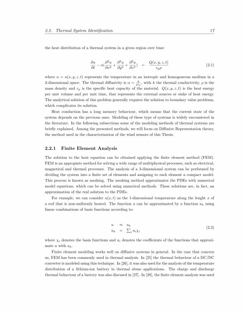
2.2. Thermal System Identification 17
the heat distribution of a thermal system in a given region over time:
∂u
∂t− α(∂
2u
∂x2 + ∂2u
∂y2 + ∂2u
∂z2 ) = Q(x, y, z, t)cpρ
(2.1)
where u = u(x, y, z, t) represents the temperature in an isotropic and homogeneous medium in a3-dimensional space. The thermal diffusivity is α = k
ρcp, with k the thermal conductivity, ρ is the
mass density and cp is the specific heat capacity of the material. Q(x, y, z, t) is the heat energyper unit volume and per unit time, that represents the external sources or sinks of heat energy.The analytical solution of this problem generally requires the solution to boundary value problems,which complicates its solution.
Heat conduction has a long memory behaviour, which means that the current state of thesystem depends on the previous ones. Modeling of these type of systems is widely encountered inthe literature. In the following subsections some of the modeling methods of thermal systems arebriefly explained. Among the presented methods, we will focus on Diffusive Representation theory,the method used in the characterization of the wind sensors of this Thesis.
2.2.1 Finite Element Analysis
The solution to the heat equation can be obtained applying the finite element method (FEM).FEM is an appropiate method for solving a wide range of multiphysical processes, such as electrical,magnetical and thermal processes. The analysis of a 3-dimensional system can be performed bydividing the system into a finite set of elements and assigning to each element a compact model.This process is known as meshing. The meshing method approximates the PDEs with numericalmodel equations, which can be solved using numerical methods. These solutions are, in fact, anapproximation of the real solution to the PDEs.
For example, we can consider u(x, t) as the 1-dimensional temperature along the lenght x ofa rod that is non-uniformly heated. The function u can be approximated by a function uh usinglinear combinations of basis functions according to:
u ≈ uh
uh =∑i uiχi
(2.2)
where χi denotes the basis functions and ui denotes the coefficients of the functions that approxi-mate u with uh.
Finite element modeling works well on diffusive systems in general. In the case that concernus, FEM has been commonly used in thermal analysis. In [25] the thermal behaviour of a DC/DCconverter is modeled using this technique. In [26], it was also used for the analysis of the temperaturedistribution of a lithium-ion battery in thermal abuse applications. The charge and dischargethermal behaviour of a battery was also discused in [27]. In [28], the finite element analysis was used

18 Chapter 2. Thesis Background
for automatically extract a compact thermal model of a test power module. Thermal wind sensor’sbehaviour has also been analyzed with 3-dimensional FEM models, as in the case of [29], where thethermal-mechanical reliability of the package of a MEMS thermal wind sensor was presented.
However, simulating a finite element model requires knowing all the thermal characteristics(specific heat, thermal conductivity, density) and to set boundary conditions of the studied ther-mal system. Hence, it requires many prior experiments for thermal characterization. In spite ofthis, non-ideal boundaries, nonlinear dynamical behaviours and exact geometries from the thermalsystem have to be taken into account in the analysis. Besides, processing is usually computerintensive due to the large modeling size.
2.2.2 Thermal Equivalent Circuit Models
For the analysis of a thermal system, an electrical analogue where temperature is alike to voltageand power is alike to current, can be used. In a thermal system, when power is injected into theheat sources, the resulting temperature variation is measured. The complex thermal impedance,Zth, is the transfer function that relates the power and temperature in the frequency domain asfollows:
Zth(ω) = T (ω)Q(ω) (2.3)
where T (ω) is the output temperature, Q(ω) is the input power and ω is the angular frequency.
Physically derived lumped parameter models
The lumped element model or lumped parameter model, simplifies the behaviour of a spatiallydistributed system into a topology of discrete entities. The PDEs of the physical system arereduced to ordinary differential equations (ODE)s with a finite number of parameters. Thesetypes of thermal equivalent circuits are designed to match the physical structure of a system.The system is considered a set of thermal homogeneous regions (or lumps) which are modeledas capacitors (akin to heat capacity). The lumps are interconnected with their neighbours usingresistors (akin to thermal resistances). The heat dissipation is modeled as a current source thatresults in heat flux (analogue to electric current) flowing through the equivalent circuit and givingrise to a temperature difference (analogue to voltage) across components [30]. The result of thismodeling is referred as a lumped parameter model. In [31], a thermal circuit anologue was presented,where an inductor for power electronic systems was modeled. In [32], the temperature estimation ofinterior permanent magnet synchronous motors was done using these thermal circuit equivalents.In the semiconductors field, in [22], the self-heating effect in MOSFETs was modeled with thelumped modeling methodology.
Equivalent circuit thermal analogues
The most typical topologies used in thermal modeling are the Cauer and Foster based networks.These networks, are mathematically identical in their one-port form [33]. Whilst the Cauer network

2.2. Thermal System Identification 19
Figure 2.6: Cauer thermal equivalent circuit [30].
is closer to the physical form of the thermal circuit form because each node represents a real tem-perature, in the Foster network, only the the overall temperature behaviours between the measuredpoints can be guaranteed [34]. Besides, Cauer networks are much more general due to the factthat Foster networks can only model self-impedance as they are an only one-port networks [30]. InFigures 2.6 and 2.7 the classical Cauer and Foster networks are shown.
The Cauer network reflects the real physical setup of the thermal device based on thermalcapacitances with intermediary thermal resistances. In order to build a model of a complete thermalsystem, the system is first divided into single material blocks, each of which is assigned a thermalresistance and capacitance. The complete system model is formed by interconnecting these blocksand inserting heat sources and ambient connections as appropriate. Typically, each single materialis modeled as a single RC element, which can also be done in 3-dimensional geometries. Thesenodes allow access to internal temperatures of layers of the material, and therefore, they havea physical significance and represent the temperature at a physical location. Foster network, incontrast, is independent of the internal structure of the material and the individual RC elements ofthe circuit do not represent any physical property, as they only represent a time constant presentin the network [30].
Figure 2.7: Foster thermal equivalent circuit [30].

20 Chapter 2. Thesis Background
Figure 2.8: Norton equivalent circuit of the thermal circuit between heat source x and measure-ment point y [36].
Although a variety of thermal networks can be used, they can all be simplified into a Nortonequivalent circuit with frequency dependant impedance. (See Figure 2.8) [35].
It can be observed that the increase of temperature at y occurs due to heat source x and it isΘy = Zthx 7−→yQx. The temperature at y due to all heat sources is calculated by superposition:
Θy =∑x
Zthx7−→yQx (2.4)
where the thermal transfer impedance Zthx7−→y is the cross-coupling between x and y. Once it isidentified, cross-coupling characteristics can be used to predict and model the temperature at eachsystem element due to the power dissipations in all the elements.
Equivalent circuit thermal analogues have been widely used. In [37] a HEV/EV battery thermalmodel using a Foster network is proposed. In [38] an electrical analogue of a voltage source convertermodule is used to estimate the junction temperatures of semiconductor devices. In [39], the Cauernetwork is proposed to obtain the nonlinear compact thermal model of power semiconductor devices.Similarly in [40], thermal impedance spectroscopy is used to assess the required number of the Cauernetwork elements to model a single material block. In [36] the thermal cross-coupling responsesbetween the multiple elements of a thermal system are obtained based on a Norton equivalentcircuit.
2.2.3 First Principles Model Derivation
From the mathematical first principles, the thermal analysis of a system can also be performed.This approach usually relies on solving the heat equation given in equation (2.1). For example,in [41], the heat equation was applied to obtain the physical model of a power electronic modulewith the intention of predicting the temperature response due to cross-coupling between devices.In [41] and [42] the thermal models based on the Fourier series are an analytical solution to the3-dimensional heat equation, where the solution uses the Fourier cosine series expansion to reducethe mathematical complexity. In [43], a 2-dimensional physical model for power bipolar devices,such as IEGT (injection-enhanced gate transistor) devices, is obtained by solving the diffusion

2.2. Thermal System Identification 21
Figure 2.9: Normalised Discrete Fourier Transform (DFT) of a PRBS sequence showing the flatregion up to the band limit[50]
equation. Although it is an effective method to model thermal effects, it can be quite complexmathematically.
2.2.4 Pseudo Random Binary Sequences in System Identification
This subsection is intended to explain a type of input signals very useful in thermal identificationanalysis.
Pseudo Random Binary Sequence (PRBS) techniques are an appropriate alternative to stepresponse testing because they have proven to be noise resilience in thermal identification problems[44, 45] thanks to the wide frequency spectrum of these type of signals. They have been usedin system identification for many decades. In [46] an in-depth analysis of the technique and itsapplication is presented. This technique has been applied to a variety of applications, includingparameter estimation in electrical generators [47], testing digital-to-analogue converters [48], andmodeling of batteries [49].
PRBSs are finite-lenght predetermined signals of pseudo aleatory ’0’s and ’1’s (or two predefined
Figure 2.10: Example of the implementation of a n = 4-bit PRBS using a linear-shift feedbackregister [49]

22 Chapter 2. Thesis Background
0 100 200 300 400 500 600 700 800 900 1000
time [s]
0
1P
RB
S
Figure 2.11: Time domain representation of 1000s of a 10-bit PRBS signal. This is the signalemployed in the simulation of the Cole-Cole model response of Figure 2.14.
levels). These signals can be synthesized using linear-shift feedback registers of length n by takingthe exclusive-NOR from several taps. For an n-bit shift register, the maximum sequence length ofthe signal is N = 2n − 1. These kinds of signals have an almost flat spectrum (see Fig. 2.9) overthe band of frequencies given by equation 2.5 [36]:
ωpN≤ ω ≤ ωp
2.3 (2.5)
where ω is the valid frequency band, ωp is the clock frequency of the PRBS and N is the numberof periods of ωP that are present in a single frequency. By applying this signal as an input powerwaveform to a thermal system and measuring the resulting temperature waveform, the system canbe characterized over the frequency band. In this way, the response of the system can be determinedover a range of frequencies simultaneously. In Figure 2.10 and example of the implementation of an = 4-bits PRBS is shown. In 2.11 an example of the time domain of this type of signals can beobserved.
2.2.5 Diffusive Representation
The Diffusive Representation (DR) was first introduced for numerical simulation of complex dy-namics in [51] and extended to a general framework in [52, 53, 54]. This dynamic representationrevealed to be convenient for analysis as well as modeling and control issues, but in particular,when long-memory dynamics are present (as in [55, 56, 57, 58]). Diffusive realization makes it welladapted to various problems, thanks to the nice properties of diffusion equations which allow theconstruction of finite-dimensional approximate state realizations simple, stable and accurate at thesame time. In this Thesis, only the discretized version of the diffusive representation is presented,which can be seen as a suitable restriction of the general theory. This version is encountered in mostof the bibliography where diffusive representation is used for system modeling [59, 60, 61, 62, 63].It is known that this mathematical tool is appropiate for for approximation of fractional-order sys-tems in practical implementations, such as thermal [62, 64, 65] or electrical [59, 66, 67] ones. Thismethod allows the description of a physical phenomena based on diffusion using state-space modelsof arbitrary order.
The main interest of this modeling method for this Thesis resides in the fact that this approach
2.2. Thermal System Identification 23
has been proven to be very suitable in thermal identification. It has been the method employed inthe thermal characterization of the sensors described in 2.1.6 and 2.1.4 and explained in chapters3 and 4. Furthermore, it has been the method employed to characterize the charge trapped in thedielectric layer of a MEMS device and described in 3.4. The theoretical grounds about diffusivereperesentation are explained below.
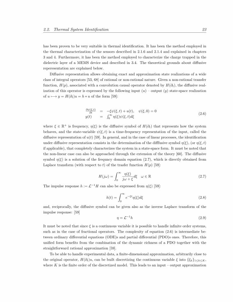
Diffusive representation allows obtaining exact and approximation state realizations of a wideclass of integral operators [53, 68] of rational or non-rational nature. Given a non-rational transferfunction, H(p), associated with a convolution causal operator denoted by H(∂t), the diffusive real-ization of this operator is expressed by the following input (u) – output (y) state-space realizationof u 7−→ y = H(∂t)u = h ∗ u of the form [59]:
∂ψ(ξ,t)∂t = −ξψ(ξ, t) + u(t), ψ(ξ, 0) = 0
y(t) =∫∞
0 η(ξ)ψ(ξ, t)dξ(2.6)
where ξ ∈ R+ is frequency, η(ξ) is the diffusive symbol of H(∂t) that represents how the systembehaves, and the state-variable ψ(ξ, t) is a time-frequency representation of the input, called thediffusive representation of u(t) [59]. In general, and in the case of linear processes, the identificationunder diffusive representation consists in the determination of the difffusive symbol η(ξ), (or η(ξ, t)if applicable), that completely characterizes the system in a state-space form. It must be noted thatthe non-linear case can also be approached through the extension of the theory [60]. The diffusivesymbol η(ξ) is a solution of the frequncy domain equation (2.7), which is directly obtained fromLaplace transform (with respect to t) of the trasfer function H(p) [59]:
H(jω) =∫ ∞
0
η(ξ)jω + ξ
dξ ω ∈ R (2.7)
The impulse response h := L−1H can also be expressed from η(ξ) [59]:
h(t) =∫ ∞
0e−ξtη(ξ)dξ (2.8)
and, reciprocally, the diffusive symbol can be given also as the inverse Laplace transform of theimpulse response: [59]
η = L−1h (2.9)
It must be noted that since ξ is a continuous variable it is possible to handle infinite order systems,such as in the case of fractional operators. The complexity of equation (2.6) is intermediate be-tween ordinary differential equations (ODE)s and partial differential (PDO)s ones. Therefore, thisunified form benefits from the combination of the dynamic richness of a PDO together with thestraightforward rational approximation [59].
To be able to handle experimental data, a finite-dimensional approximation, arbitrarily close tothe original operator, H(∂t)u, can be built discretizing the continuous variable ξ into ξk1≤k≤K ,where K is the finite order of the discretized model. This leads to an input – output approximation
24 Chapter 2. Thesis Background
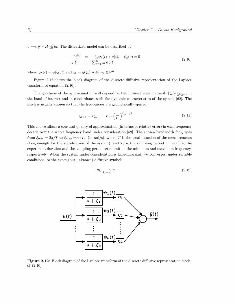
u 7−→ y ≈ H( ddt )u. The discretized model can be described by:
dψk(t)dt = −ξkψk(t) + u(t), ψk(0) = 0
y(t) =∑Kk=1 ηkψk(t)
(2.10)
where ψk(t) = ψ(ξk, t) and ηk = η(ξk) with ηk ∈ RK .
Figure 2.12 shows the block diagram of the discrete diffusive representation of the Laplacetransform of equation (2.10).
The goodness of the approximation will depend on the chosen frequency mesh ξk1≤k≤K , inthe band of interest and in concordance with the dynamic characteristics of the system [62]. Themesh is usually chosen so that the frequencies are geometrically spaced:
ξk+1 = rξk, r =(ξKξ1
)( 1K−1 ) (2.11)
This choice allows a constant quality of approximation (in terms of relative error) in each frequencydecade over the whole frequency band under consideration [59]. The chosen bandwidth for ξ goesfrom ξmin = 2π/T to ξmax = π/Ts, (in rad/s), where T is the total duration of the measurements(long enough for the stabilization of the system), and Ts is the sampling period. Therefore, theexperiment duration and the sampling period set a limit on the minimum and maximum frequency,respectively. When the system under consideration is time-invariant, ηK converges, under suitableconditions, to the exact (but unknown) diffusive symbol:
ηK −→K→∞
η (2.12)
Figure 2.12: Block diagram of the Laplace transform of the discrete diffusive representation modelof (2.10)

2.2. Thermal System Identification 25
Which means that if the frequency mesh is sufficiently dense, it is possible to describe with arbitraryaccuracy the response of any fractional system.
The inference of the diffusive symbol is done from the experimental data. Considering that themeasurement data is distributed in a temporal mesh, [tn]1≤n≤N ∈ R+, we can define the matrixA = [ψk(tn)] and the output vector of measurements as YT = [y(t0), . . . , y(tn), . . . , y(tN )]. Takingthis notation into account, the solution to the identification problem is found solving the finitedimensional least squares problem formulated by [62]:
minη∈RK
||Aη −Y||2 (2.13)
that is classically solved by the standard pseudo-inversion method:
η = [A∗A]−1A∗Y (2.14)
The identfication problem is often ill-conditioned because the matrix [A∗A] is close to a non-invertible one. This problem is usually solved by adding a small penalization term ε > 0 to theequation: [62]
η = [A∗A + εI]−1A∗Y (2.15)
where I is the identity matrix and the parameter ε is chosen as small as possible as long as ηremains quasi-insesitive to important relative variations of ε. In practice, very small values of ε aresufficient to stabilize the problem.
It has to be mentioned that when resolving numerically the integral of equation (2.6), to dealwith numerical approximations, standard quadrature methods have to be used. One method isbased on the use of linear interpolation [59]:
ηk = η(ξk)∫ +∞
0Λk(ξ)dξ = η(ξk)ξk+1 − ξk−1
2 (2.16)
with Λk the classical interpolation function defined by:
Λk(ξ) =
0, for ξ ≤ ξk−1 or ξ ≥ ξk+1ξ−ξk−1ξk−ξk−1
, for ξk−1 < ξ < ξkξk+1−ξξk+1−ξk , for ξk < ξ < ξk+1
(2.17)
where for k = 1 and k = K, fictious points are introduced: ξ0 = ξ1/r and ξK+1 = rξK , being r theratio of the geometric sequence of the mesh of ξ defined in (2.11). Regarding to the identificationproblems of this Thesis, to solve the integral from equation (2.6) a logarithmic change of variablehas been used due to the fact that ξ variable has chosen to be spaced geometrically. Specifically,ξ = 10x and dξ = ln(10)10xdx. Taking this into account, the second expression of equation (2.6)

26 Chapter 2. Thesis Background
becomes:
y(tn) =∫ x1x0η(10x)ψ(10x, t)ln(10)10xdx ≈
∑Kk=1 ηkψk(tn)λk (2.18)
Therefore, the term λk divides the inferred diffusive symbol, ηk = ηkλk
, where λk = ln(10)log(r)ξk.
For the problems proposed in the work carried out during this Thesis, we have to considerthe general case where ηk is time-varying, i.e. wind changing conditions in a wind sensor. Forthis reason, during the research work it was necessary to reformulate the discretized approch fromequation (2.10) to maintain the linearity of the model. The equations developed during the Thesisto treat the time-varying case are presented below.
ψ(n)k (t) = 0 t ∈ [t0, tn]ψ
(n)k (t) = −ξkψ(n)
k + u(t) t ∈ [tn, tn+1]ψ
(n)k (t) = −ξkψ(n)
k t > tn+1
(2.19)
y(t) =∑n,k η
(n)k ψ
(n)k (t) +
∑Kk cke
−ξk(t−t0)
where η(n)k ∈ RK is the diffusive symbol associated to the conditions of the system in the n-th
interval in t ∈ [tn, tn+1]. In this general formulation, the state of the system at the beginning ofthe measurements is taken into account thanks to ck ∈ RK that represents the initial conditionsof the system, at t = t0. The time intervals are a discretization of time for which the diffusivesymbols can be considered constant in a experiment. From an experiment, the discrete numberof diffusive symbols that will be obtained is J . For example, in the case where a wind sensoris being characterized, J will be the number of wind velocities applied in the experiment. Eachevent, ajj=1,...,J , represents the time interval of an experiment where the diffusive symbol η(n)
k isconstant.
The solution again to this identification problem is found solving the finite least squares problemfrom equation (2.13), but in this general case, matrix A is of the form shown in equation (2.20)and ηT is that of equation (2.21):
A =
∑
n:g(n)=a1
ψ(n)1 (t0) . . .
∑n:g(n)=a1
ψ(n)K
(t0), . . .∑
n:g(n)=aJ
ψ(n)1 (t0) . . .
∑n:g(n)=aJ
ψ(n)K
(t0), [1]k
.... . .
......
.... . .
......∑
n:g(n)=a1
ψ(n)1 (tF ) . . .
∑n:g(n)=a1
ψ(n)K
(tF ), . . .∑
n:g(n)=aJ
ψ(n)1 (tF )] . . .
∑n:g(n)=aJ
ψ(n)K
(tF ), [e−ξk(tF−t0)]k]
(2.20)
for a experiment with t ∈ [t0, tF ]. The function g(n) returns the aj event at every n-th time intervalin t ∈ [tn, tn+1]n=0,...,N at which η(n)
k is constant. Returning to the wind sensor example, g(n) willreturn the wind applied at every interval n. In the last column of matrix (2.20), [1]k ∈ RK is an

2.2. Thermal System Identification 27
all ones vector and [e−ξk(t−t0)]k = [e−ξ1(t−t0), . . . , e−ξK(t−t0)]. The diffusive symbol vector that isgoing to be inferred is of the form of equation (2.21):
ηT = [[ηa11 , . . . , ηa1
K ]T , . . . , [ηaJ1 , . . . , ηaJK ]T , [c1, . . . , cK ]T ] (2.21)
where [ηajk ]T is the diffusive symbol corresponding to the aj event. The measurements vector, YT ,remains as in (2.13), and the solution to the inference problem is classically given by (2.14).
In this Thesis, the time-varying thermal dynamics models of a thermal system are extractedfrom open-loop measurements using diffusive representation. From a single experiment, wherethe thermal conditions (or events) are continuously changing (i.e. in a wind sensor, the windspeed is switched between several wind velocities) the models that represent the behaviour ofthe system under that conditions can be obtained. The diffusive symbols corresponding to eachevent, aj (for j = 1 . . . J), are inferred from a single experiment, with t ∈ [t0, tF ]. These eventsare distributed in a uniformly random sequence along the experiment. Each event occurs in atime interval t ∈ [tn, tn+1]n=0,...,N , where N is the total number of events, such that, N J .(For example, in a wind sensor, J will be the number of wind velocities for which the sensor willbe characterized, and N will be the number of times the wind velocity has changed). All theevents have a short duration ∆tn = (tn+1 − tn), where ∆tn tF , for all n. In the meantime,a PRBS heating current is applied to the heat sources of the system in open-loop, with a periodTPRBS ∆tn tF , while the temperature of different components of the system is sensed with aperiod Ts. As mentioned before, in the subsection 2.2.4, PRBS signals allow to improve the qualityof the fittings in presence of noise due to their wide spectrum. The frequency mesh for the time-varying case remains geometrically spaced, but in this case the minimum frequency is set accordingto J . Now, ξmin = (2πJ) /T [in rad/s] while the maximum frequency is the same, ξmax = π/Ts.
The diffusive representation framework can be generalized to the MIMO (Multiple Input/ Mulit-ple Output) case. In this case, the couplig between several heat sources of a system can be analyzed.Taking this into account, cross-heating models can be constructed. These models reproduce theeffect of injecting a power into heat sources in parts of the structure different from the one in whichthe temperature is sensed. The linearity assumption of the models enables to build the thermalmodel by parts [62]. A detailed description of the equations governing this effect can be encounteredin chapter 4.
In practice, a small value of the model order, K, is mostly sufficient to get a good aproximation.From the literature [59, 62] and the experimentality, it has been observed that low order modelsare enough to obtain a good fitting of the experimental data and to recover the analytical diffusivesymbol. It is usually observed that increasing the model order does not improve the root meansquare error between the experimental and the fitting data beyond a certain order value [67].
The main advantage of diffusive representation is that it is possible to obtain reduced ordermodels of long-memory systems without great computational load. Besides, these state-space mod-els are very well suited to describe the behaviour of diffusive systems under nontrivial controls,such as sliding mode controllers (see section 2.3). Therefore this has been the method employedin the characterization of the systems related to the content of this Thesis. In sections 3.1 and

28 Chapter 2. Thesis Background
10-3 10-2 10-1 100 101 102 103
frequency [Hz]
0
0.05
0.1
0.15
0.2
()
Cole-Cole
Figure 2.13: Analytical diffusive symbol of Cole-Cole dielectric model for α = 0.5 and τ0 = 1.
3.3 the thermal dynamics of the UPC 3-D hot sphere anemometers, explained at 2.1.6, have beencharacterized.
2.2.6 Cole-Cole Example
As a numerical example, the Cole-Cole model is presented in this subsection. This work wasnecessary in the beginning of the research work, to help understand the diffusive modeling theoryand to find the best input signal to obtain the best quality of the thermal system identification.
The relaxation properties of a dielectric material, as polymers, can be described in the frequencydomain by the Cole-Cole equation. This model, introduced in 1941 (see [69, 70]), is still used torepresent the impedance of biological tissues, to describe relaxation properties in polymers andfor representing anomalous diffusion in disordered systems [71, 72, 73]. The empirical Cole-Cole
0 100 200 300 400 500 600 700 800 900 1000
time (s)
0
0.2
0.4
0.6
0.8
1
y(t)
step
Cole-Cole simulation
0 20[s]
0
0.5
1
0 100 200 300 400 500 600 700 800 900 1000
time (s)
0
0.2
0.4
0.6
0.8
1
y(t)
PRBS
Cole-Cole simulation
100 120(s)0
1
Figure 2.14: Simulation of Cole-Cole model response for α = 0.5 and τ0 = 1. Left: Response ofthe model with the unitary step input signal. Right: Response of the model with a PRBS inputsignal.
2.2. Thermal System Identification 29
10-3 10-2 10-1 100 101 102 103
frequency [Hz]
0
0.05
0.1
0.15
0.2(
)step
Cole-Cole analyticalCole-Cole DR step
10-3 10-2 10-1 100 101 102 103
frequency [Hz]
0
0.05
0.1
0.15
0.2
()
PRBS
Cole-Cole analyticalCole-Cole DR PRBS
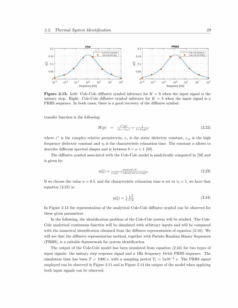
Figure 2.15: Left: Cole-Cole diffusive symbol inference for K = 8 when the input signal is theunitary step. Right: Cole-Cole diffusive symbol inference for K = 8 when the input signal is aPRBS sequence. In both cases, there is a good recovery of the diffusive symbol.
transfer function is the following:
H(p) = ε∗(p)(εs−ε∞) = 1
1+(τ0p)α (2.22)
where ε∗ is the complex relative permittivity, εs is the static dielectric constant, ε∞ is the highfrequency dielectric constant and τ0 is the characteristic relaxation time. The constant α allows todescribe different spectral shapes and is between 0 < α < 1 [59].
The diffusive symbol associated with the Cole-Cole model is analytically computed in [59] andis given by:
η(ξ) = sin(απ)/π(τ0ξ)−α+2cos(απ)+(τ0ξ)α (2.23)
If we choose the value α = 0.5, and the characteristic relaxation time is set to τ0 = 1, we have thatequation (2.23) is:
η(ξ) = 1π
√ξ
1+ξ(2.24)
In Figure 2.13 the representation of the analytical Cole-Cole diffusive symbol can be observed forthese given parameters.
In the following, the identification problem of the Cole-Cole system will be studied. The Cole-Cole analytical continuous function will be simulated with arbitrary inputs and will be comparedwith the numerical identification obtained from the diffusive representation of equation (2.10). Wewill see that the diffusive representation method, together with Pseudo Random Binary Sequences(PRBS), is a suitable framwework for system identification.
The output of the Cole-Cole model has been simulated from equation (2.24) for two types ofinput signals: the unitary step response signal and a 1Hz frequency 10-bit PRBS sequence. Thesimulation time has been T = 1000 s, with a sampling period Ts = 5x10⁻⁴ s. The PRBS signalemployed can be observed in Figure 2.11 and in Figure 2.14 the output of the model when applyingboth input signals can be observed.

30 Chapter 2. Thesis Background
0 100 200 300 400 500 600 700 800 900 1000
time [s]
0
0.2
0.4
0.6
0.8
1
y(t)
step
simulationfitting - step
0 100 200 300 400 500 600 700 800 900 1000
time [s]
0
0.2
0.4
0.6
0.8
1
y(t)
PRBS
simulationfitting - PRBS
0 20[s]
0
0.5
1
100 120[s]0
1
Figure 2.16: Left: Cole-Cole simulation data (in blue) Vs Fitting data (in red) when the inputsignal is the unitary step. Right: Cole-Cole simulation data (in blue) Vs Fitting data (in red) whenthe input signal is a PRBS sequence.
10-3 10-2 10-1 100 101 102 103
frequency [Hz]
-0.05
0
0.05
0.1
0.15
0.20.2
()
step
Cole-Cole analyticalCole-Cole DR step
10-3 10-2 10-1 100 101 102 103
frequency [Hz]
-0.05
0
0.05
0.1
0.15
0.2
()
PRBS
Cole-Cole analyticalCole-Cole DR PRBS
Figure 2.17: Cole-Cole diffusive symbol inference for K = 8 when the simulation data is addedwith gaussian noise. Left: when the input signal is the unitary step. Right: when the input signalis a PRBS sequence. There is a better recovery in the PRBS case.
From the simulation data of Figure 2.13 and the diffusive representation theory, the Cole-Colediffusive symbol has been reconstructed, using the finite representation of equation (2.10). For theinference, we choose a model order of K = 8 and set the minimum and maximum frequencies tofmin = 1/T = 1x10⁻³Hz and fmax = 1/2Ts = 1x10³ Hz respectively. In Figure 2.15 we can observethat for both input signals, the unitary step and the PRBS, the diffusive symbol is well recoveredwith 8 poles. In both cases, the fitting of the output signal is good-matched with the simulationdata (see Figure 2.16). As it can be observed, both fittings are indistinguisable from the simulationdata.
At a first glance it may seem that the fact of applying a step or a PRBS signal does not makeany difference in the system identification. However, it has to be noted that in the previous examplethe simulation data was obtained from the ideal noiseless case. If we add white gaussian noise tothe simulation data, the recovery of the diffusive symbol in the case where the input signal is theunitary step does not faithfully represent the analytical case and even has one negative value. Onthe contrary, the recovered diffusive symbol in the case where the input signal is a PRBS sequence,

2.3. Sliding Mode Controllers: Sigma–Delta Modulation Approach 31
0 100 200 300 400 500 600 700 800 900 1000
time [s]
-0.5
0
0.5
1
1.5
y(t)
step
simulationfitting - step
0 100 200 300 400 500 600 700 800 900 1000
time [s]
-0.5
0
0.5
1
1.5
y(t)
PRBS
simulationfitting - PRBS
100 120[s]0
1
0 20[s]
0
1
Figure 2.18: Fitting of the Cole-Cole output when the simulation data is added with whitegaussian noise. Letf: simulation data (in blue) Vs Fitting data (in red) when the input signal is theunitary step. Right: Cole-Cole simulation data (in blue) Vs Fitting data (in red) when the inputsignal is a PRBS sequence.
remains undisturbed. Nevertheless, in both cases (step and PRBS input signal), the fitting datahas very good agreement with the noise-added simulation data. These results are observable inFigures 2.17 and 2.18.
As mentioned before, and as deduced from Figures 2.15 and 2.17, the identification is moreresilient to noise when the input signal is a PRBS sequence. Moreover, when resolving the leastsquares problem formulated in equation (2.14), the solution is improved as the case of an ill-conditioned pseudo-inverse matrix is minimized because the input data is much more uncorrelated.For these reasons, in all the experiments carried out for system characterization of this Thesis,PRBS input signals have been employed successfully.
2.3 Sliding Mode Controllers: Sigma–Delta Modulation Ap-proach
The Sliding Mode Control (SMC) technique is, fundamentally, a state space-based discontinuousfeedback control technique. It is an efficient tool to design robust controllers for complex high-ordernonlinear dynamic systems operating under uncertainty conditions [74]. The principal advantagesof sliding mode control are order reduction, decoupling design procedures, disturbance rejection andtheir low sensitivity to systems’ parameter variation, which reduces the complexity of the feedbackdesign. This technique has been proved to be appropiate for a wide range of problems, such asrobotics, process control and vehicle and motion control [74, 75, 76, 77].
In the wind sensor system presented in section 2.1.6, a closed thermal feedback loop based onthermal sigma-delta (Σ–∆) modulation is used to keep constant the temperature in the sensor.These kinds of modulators [78] have been used for decades as analog to digital converters and alsoas closed-loop control circuit topologies for inertial or thermal sensors and actuators [5, 79].
With respect to the purpose of this Thesis, the thermal dynamics of the state variables of the

32 Chapter 2. Thesis Background
proposed wind sensors of section 2.1.6, under closed-loop control, have been analyzed with the toolsof sliding mode controllers. It must be noted that the state variables of the thermal filter followa sliding motion on the control surface determined by Temperature = constant. In this regard,no specific design of a sliding mode controller has been made, but the analysis of the resultingdynamics is made using the tools of equivalent control typical of sliding mode controllers.
2.3.1 Sigma-Delta Modulation
As it has been metioned previously, sigma-delta modulators are a class of analog to digital (A/D)converters that have been extensively studied [78]. Some of their principal advantages are thesimplicity and robustness in front of component mismatch. Noise shaping and the oversamplingof the input signal compensate the fact of using a very coarse quantization scheme. This allowsthis type of circuits to reach higher resolutions than in the case of other A/D converters, withoutthe use of high-precision components. Besides, they can be used in the control loop of sensors oractuators to keep constant a given variable. In this way, the closed-loop control of a given variableand an implicit analog-to-digital conversion of a given magnitude are achieved [5]. One of the mostused topologies is the first-order sigma-delta modulator shown in Figure 2.19
The topology of a first-order sigma-delta, takes the form of a negative feedback loop. Theoutput of the modulator, bn, is a digital pulse train. The output is substracted from the input toproduce the error signal, which is integrated over the sampling period. The intermediate signal, un,is then quantized to form the output signal bn. The main objective of the modulator is to minimizethe difference between the integrated binary output and the integrated input. As a result of thefeedback, the average value of the output will be a digital representation of the average value ofthe input signal. The equation governing the circuit of Figure 2.19 is the following:
un+1 = un + δ − sgn(un) (2.25)
where δ is the magnitude to convert, 0 ≤ δ ≤ 1, assumed constant. The convention for sgn(ρ) issgn(ρ) = 1 for ρ ≥ 0 and sgn(ρ) = 0 for ρ < 0. un is the value the integrator takes at t = nTs,with Ts being the sampling period. The solution to the above equation is the following [5]:
un = (u0 + (n− 1)δ)mod1− 1 + δ (2.26)
Figure 2.19: First-order sigma-delta modulator with constant input δ [5].
2.3. Sliding Mode Controllers: Sigma–Delta Modulation Approach 33
and the bitstream at the output of the modulator is
bn = δ + (u0 + (n− 1)δ)mod1− (u0 + nδ)mod1 (2.27)
Regarding to this Thesis, the sensors presented in 2.1.6 are made to operate under constanttemperature anemometry (CTA). To this effect, the temperature in the heating elements is forcedto be constant. To achieve that, the implemented sigma-delta modulator applies a modulatedpower to the heat sources of the sensor to maintain the temperature constant. In this discrete-timecontrol, at each sampling period, Ts, the current temperature of the structure, Tn = T (nTs), iscompared with the desired target temperature, ∆T , as follows:
• If Tn ≥ ∆T , then the heater is switched OFF during the following sampling period (Poff isdelivered into the heat sources).
• If Tn < ∆T , then the heater is switched ON during the following sampling period (Pon isdelivered into the heat sources).
where Pon > Poff. In order to be able to adapt the sensor to different flow and temperatureconditions, it is usual to have a quiescent power: Poff 6= 0.
2.3.2 Sliding Mode Controllers
Sliding mode controllers are nonlinear controllers that alter the dynamics of the system by applyinga discontinuous control signal so that under some conditions the system ’slides’ on a certain controlsurface to obtain the desired behaviour of the system [80, 81]. The controller is designed in orderto drive the state variables of the system into a particular surface in the state-space, named slidingsurface. Once the surface is reached, sliding mode control switches from one continuous structure toanother based on the current position in the state-space. Hence, sliding mode control is a variablestructure control method. These types of controls alter the dynamics of a nonlinear system byapplication of a high frequency switching control. The discontinuous control switches from onesmooth condition to another. This motion is called sliding mode. There are two main advantagesin sliding mode controllers. First is that the dynamic behaviour of the system may be adapted bythe particular choice of the sliding function. Secondly, the closed loop response becomes insensitiveto some particular uncertainties. In the following, the dynamics of this type of control will bestudied.
A dynamical model can be described as a unified state-space representation in a usual controlsystem:
x = f(x, u) (2.28)
where x ∈ Rn is a vector which represents the state and u ∈ Rm is the control input. It is assumedthat f(·) is differentiable with respect to x and absolutely continuous with respect to time. The

34 Chapter 2. Thesis Background
control u is a discontinuous function of the state such that:
u =
u+(x), if σ(x) > 0
u−(x), if σ(x) < 0(2.29)
where we can define σ = Sx(t), being S a surface in the state-space given by:
S = x : σ(x) = 0 (2.30)
An ideal sliding mode is said to take place on equation (2.30) if the states x(t) evolve with timesuch that σ(x(tr)) = 0 for some finite tr ∈ R+ and σ(x(t)) = 0 for all t > tr. The control u thatdrives the state variables x(t) to the sliding surface of (2.30) in finite time, and keeps them onthe surface thereafter, is called a sliding mode controller [82]. The main objective is to select anadmissible control law u such that the control surface σ(x) = 0 is reached in a finite time.
The closed loop dynamics of a system, under the control law of (2.29) in a discrete time interval[nTs, (n+ 1)Ts], is given by:
x = 1 + sgn(σ(nTs))2 f(x, u+(x)) + 1− sgn(σ(nTs))
2 f(x, u−(x)) (2.31)
In this section, the sign function is redefined as sgn(ρ) = +1 when ρ ≥ 0 and sgn(ρ) = −1 whenρ < 0. Under the infinite sampling approximation, when Ts tends to zero, the system of (2.31) canbe written as a switched system [81]:
x =
f0(x), if σ > 0
f1(x), if σ < 0(2.32)
If solutions starting nearby the surface are directed towards it, the switching surface is determinedas attractive, which guarantees the existance of a sliding region within the control surface. Thisoccurs if σσ < 0, [83], with σ computed over the system trajectories:
σ = Sx =
Sf0(x), if σ > 0
Sf1(x), if σ < 0(2.33)
The attractive sliding region, or sliding domain Ω, is given by [83]:
Ω := x ∈ Rn : Sf0(x) < 0 ∩ x ∈ Rn : Sf1(x) > 0 ∩ σ(x) = 0 (2.34)
Let us assume that the system defined in (2.32) undergoes over the switching surface with asliding motion, i.e., the sliding domain Ω is nonempty. The obtention of the ideal sliding dynamicsconsists in obtaining a solution in the sense of Filippov [83]. A solution in the sense of Filippov isobtained when the system is defined on the sliding surface as a convex linear combination of f0(x)

2.3. Sliding Mode Controllers: Sigma–Delta Modulation Approach 35
and f1(x), acting in the corresponding space region:
x = (α(x)f0(x) + (1− α(x))f1(x)) |σ(x)=0 (2.35)
for α(x) ∈ [0, 1]. This convex combination, will be such that the derivative will be tangent to thesliding surface (see right picture of Figure 2.20). This last condition implies that the time derivativeof σ(x), evaluated at any point such that σ(x) = 0, must be zero:
σ = 0 = Sx = (S (α(x)f0(x) + (1− α(x))f1(x))) |σ(x)=0 (2.36)
Taking this into account, we have that α(x) ∈ [0, 1] must be such that:
α(x) =(
Sf1(x)Sf1(x)−Sf0(x)
)|σ(x)=0
(2.37)
The function α(x) may be seen as the equivalent control, ueq, necessary to keep the system in thesliding surface. With this expression, the time evolution of the system once it has reached thesliding surface, this is, the sliding motion x, can be described as:
x = Sf1(x)f0(x)− Sf0(x)f1(x)Sf1(x)− Sf0(x) (2.38)
With respect to the work of this Thesis, the state-space models necessary to carry out the slidingmode analysis are provided from the diffusive representation modeling from section 2.2.5. Thesliding analysis will be undertaken considering the thermal sigma-delta control explained in section2.3.1 which is a case of a sliding mode controller. The infinite sampling frequency approximationis assumed for the obtention of the equivalent control.
In this case, under the infinite sampling approximation, the bitstream bn, output of the sigma-delta, may be seen as a continuous time variable:
bn −→Ts→0
b(t) = sgn(σ(t))2 (Pon − Poff) + 1
2(Pon + Poff) (2.39)
where σ(t) = ∆T − [H(∂t)b] (t). H(∂t) is the convolution causal operator and was defined in section
IntroductionSigma-Delta control of Multiexponential Systems
Sliding mode analysisConclusions
Mixed behaviour: predetermined & state-based switchingReaching vs. sliding phaseNumerical and experimental corroborationExternal disturbances: ionizing radiation
Sliding mode analysisI A control surface, S = σ(x , t) = 0, determines the discontinuous
control signal, u:
x = f (x , t) + B(x)u(t), u =
u+
i (x , t) if σi (x , t) > 0
u−i (x , t) if σi (x , t) < 0
I If the system reaches the surface, under some conditions, it slides on it:Filippov solution
Control
surface
S
Chattering
Reaching
phase
Control
surface
S
faC
f-C
f+C
Figure 2.20: Left: Description of the sliding motion. Right: Filippov solution representationwithin the control surface.

36 Chapter 2. Thesis Background
2.2.5. The discretized diffusive representation model now becomes:
dψk(t)dt
=
−ξkψk(t) + Pon, σ > 0
−ξkψk(t) + Poff, σ < 0(2.40)
If we define Ψ(t) = (ψ1(t), . . . , ψK(t)) ∈ RK , the control surface can be defined as:
σ(Ψ(t)) = ∆T − y(t) = ∆T −K∑k
ηk(t)ψk(t) (2.41)
for a time-varying system, and with ∆T the desired target temperature of the sigma-delta control.
A. Reachability conditions
The objective in the control is to place the system within the control surface σ(ψ(t)) = 0. In systemsworking at constant temperature mode, this condition is achieved when
∑Kk ηk(t)ψk(t) = ∆T .
This temperature level may or may not be reached depending on the maximum and minimim heatinjections, Pon and Poff. The system will reach the sliding surface σ(x) = ∆T−
∑Kk=1 ηk(t)ψk(t) = 0
in finite time from any initial condition Ψ(0) if:
Poff
K∑k
ηk(t)ξk
< ∆T (2.42)
and
Pon
K∑k
ηk(t)ξk
> ∆T (2.43)
This two conditions are achieved from the fact that the control surface σ = 0 divides in two partsthe state-space. For the side of the hyperplane where σ > 0, the system evolution is:
dψk(t)dt
= −ξkψk(t) + Pon (2.44)
which solution is given by:
ψk(t) = ψk(0)e−ξkt + Ponξk
(1− e−ξkt) for t > 0 (2.45)
This means that from any initial Ψ(0), such that σ(Ψ(0)) > 0, the control surface σ = 0 will bereached if the asymptotic point of this trajectory lies on the other side of the hyperplane, i.e. wehave condition (2.43) fullfilled. A similar analysis for σ < 0 will give us the condition of (2.42).

2.3. Sliding Mode Controllers: Sigma–Delta Modulation Approach 37
B. Attractive sliding region
The attractive sliding region is such that guarantees a sliding region within the control surface,under the condition σσ ≤ 0. First we must note that:
σ(Ψ(t)) =
∑Kk ηk(t)ξkψk(t)− PonΓ, σ(Ψ(t)) > 0∑Kk ηk(t)ξkψk(t)− PoffΓ, σ(Ψ(t)) < 0
(2.46)
where Γ =∑Kk ηk(t). This means that the attractive sliding region is given by:
Ω := Ψ(t) ∈ RK : Poff <1Γ
K∑k
ηk(t)ξkψk(t) < Pon ∩ σ(Ψ(t)) = 0 (2.47)
C. Sliding motion
The condition σ(Ψ(t)) = 0 gives the necessary equivalent control under a sliding motion to maintainthe temperature constant and for a system described by diffusive representation and consideringthe Filippov regularization, we have:
σ(t) = −∑Kk ηk(t)ψk(t) =
∑Kk ηk(t)(ξkψk(t)− ueq(t)) = 0 (2.48)
From this equation, the equivalent control, ueq, in the sense of Filippov, is obtained:
ueq(t) = Γ−1∑Kk ηk(t)ξkψk(t) (2.49)
Then, the dynamics of the system in the control surface (σ = 0) is determined when the equivalentcontrol is applied:
ψk(t) + ξkψk(t) = Γ−1∑Kl ηl(t)ξlψl(t) (2.50)
If the equilibrium point (ψk(t) = 0) is reached, the system takes the steady-state values:
ψQ(ξk) = uQξk
uQ = ∆T∑K
kηk/ξk
(2.51)
As mentioned before, the closed-loop dynamics of a wind sensor are being determined. There-fore, the changes in wind speed must be taken into account. The equivalent control to maintainthe desired target temperature can be predicted using the diffusive symbols inferred in a previousopen-loop characterization, therefore, the wind velocities for which the analysis is done must bethe same as the ones for which the wind sensor has already been characterized.
The first step to calculate the equivalent control is to obtain the point tc ∈ (t0, t1) at which thesystem reaches the control surface, σ = 0. From a zero initial condition, a constant u(t) = Pon is
38 Chapter 2. Thesis Background
applied till the control surface is reached. The intersection point of this initial trajectory with thesurface is the initial condition for the sliding movement on the control surface following expressions(2.49) and (2.50). Now, equation (2.50) can be expressed as:
ψk(t) = −D(t)ψ(t), t ≥ tc (2.52)
where D(t) collects the terms in equation (2.50). If the wind velocities applied to the sensor are keptconstant within the time intervals ∆tn = (tn+1− tn), for n = 0, . . . N , being the N time intervals ofwind applied, D(t) can be considered a piecewise constant and therefore for t ∈ [tn, tn+1] we have:
ψ(t) = e−D(n)(t−tn)ψ(tn) (2.53)
where:
D(n) = Γ−1
η
(n)1 ξ1 − Γξ1 . . . η
(n)K ξK
.... . .
...η
(n)1 ξ1 . . . η
(n)K ξK − ΓξK
with η
(n)k the diffusive symbol of the sensor working under the wind of the n-th time interval.
Replacing equation (2.53) in the equivalent control expression of equation (2.49) we reach to:
ueq(t) = H(t)ψ(tc) (2.54)
where:
H(tn) = Γ−1K∑k
ηk(t)ξke−D(n)(tn−tn−1)e−D
(n−1)(tn−1−tn−2) · · · eD(1)(t1−tc) (2.55)
where it has been assumed that t1 > tc.
D. Effect of external disturbances and model uncertainties
Model uncertainties and external disturbances in the system (i.e. wind velocity changes in thewind sensor) can be represented by an additional term, Θ(Ψ, t) = (Θ1(Ψ, t), . . . ,ΘK(Ψ, t))T . SinceΨ(0) = 0, we have that the wind sensor thermal system can be expressed as:
ψk(t) = −ξkψk(t) + ηk2 (Poff + Pon)
+ηk2 (Pon − Poff)sgn(σ(Ψ(t))) + θk(Ψ, t)
σ(Ψ(t)) = ∆T −∑Kk ψk(t)
(2.56)
Assuming the sliding region is taking place, this is σ = 0, the equivalent control is now:
ueq =∑Kk ξkψk(t)− Γ
2 (Poff + Pon)− χ(Ψ, t)Γ2 (Pon − Poff)
∈ [−1, 1] (2.57)

2.4. Dielectric Charging in Contactless MEMS 39
with χ(ψ, t) =∑k θk(ψ, t). The new dynamics in the control surface is therefore determined by:
ψk(t) = −ξkψk(t) + ηk2 (Poff + Pon) + θk(ψ, t)
+ηkΓ[∑
l ξlψl(t)−Γ2 (Pon + Poff)− χ(Ψ, t)
] (2.58)
The disturbances can be decomposed in a matched and a mismatched component [81]. Inthe case of a matched disturbance, θk(t) − ηk
Γ χ(ψ, t) = 0, the disturbance is proportional to thediffusive symbol, i.e. θk(ψ, t) = βηk for some β ∈ R. Under this condition, the control methodwill be able to handle successfully the disturbances with a fast (almost instantaneous) response,since the dynamics of the system on the control surface would remain undisturbed. However, inthe general case where a mismatched component is present, any disturbance will generate a changein the dynamics of the system on the control surface, therefore generating a slow dynamics in theequivalent control. Usually, the dynamics triggered by a mismatched component is expected to beof the same order as the one in the open-loop response, i.e., slow. One way of ensuring that any dis-turbance is a matched disturbance is the very simple case of having one state variable. This meansthat in a general case, it is very convenient to have only one significant state variable on the system.
In the literature, both tools, sliding mode controllers and diffusive representation, have been usedtogether recently in numerical applications, as in [84] where sliding mode control laws are designedfor fractional oscillators or in [85] where chaos control is given to illustrate the efficiency of the pro-posed method with first and second order sliding mode controllers. However, this Thesis presentsa practical application, as both tools have been applied together in wind sensing thermal analysis,where it has been shown that the diffusive symbols from diffusive representation modeling of section2.2.5 allow to predict the system behaviour under closed-loop operation control in the presence ofwind variations.
2.4 Dielectric Charging in Contactless MEMS
Microelectromechanical systems (MEMS) is the technology that underlies the miniaturized mechan-ical and electro-mechanical elements that are made using the techniques of microfabrication. Thesedevices are present in a great variety of applications such as communications, medicine or biotech-nology. They are widely used as sensors (for sensing magnitudes such as pressure, temperature,chemical, magenetical or inertial forces) and as actuators.
For the development of this Thesis, the charge trapped in the dielectric layer of a contactlesselectrostatically actuated MEMS has been characterized for different voltage actuations. Thesedevices, used as varactors, resonators or switches in a large set of applications, suffer from theundesired effect of parasitic charge trapped in the dielectric layers. The problems associated tothis effect go from pull-in voltage drifts, capacitance-voltage (C(V )) curve shifts, to even stictionof moveable parts.
In order to study the time evolution of the trapped charge, the generic MEMS topology of

40 Chapter 2. Thesis Background
Figure 2.21, with movable-top and fixed-bottom electrodes, can be considered. The dynamics ofthe deflection of the upper electrode, x(t), can be described by a mass-spring-damper ordinarydifferential equation [86]:
mx(t) + bx(t) + kx(t) = Fel(x, t) (2.59)
where m is the mass of the upper electrode, b is the damping factor, k is the spring coefficient andFel is the electrostatic force applied to the movable electrode described by [86]:
Fel(t) = C(t)2
2Aε0
(V − Qd
Cd
)2(2.60)
where C(t) is the total capacitance of the MEMS, Qd is the total amount of charge trapped inthe dielectric layer, ε0 is the permitivity of the air, and Cd = Aε0εd/d is the capacitance of thedielectric, with εd the relative dielectric constant of the material, A the device area and d thedielectric layer thickness. The electrostatic force, Fel, is proportional to the square of the termdefined as voltage shift: Vsh = Qd/Cd, from which the net charge, Qd, can be inferred. The C(V )characteristic of the device is a function centered at this voltage, V = Vsh, and for the operationbelow pull-in, the C − V curve can be approximated by a parabolic function [87, 88]:
C(V, t) = α(V − Vsh(t))2 + C0 (2.61)
where α is the second order coefficient of the parabola, fitted for each device, and C0 is the minimumcapacitance value of the curve. It must to be said that C0 may present slow time dependances,C0(t), due to changes in temperature, humidity or in the uniformity of charge distribution [89, 90].
In order to avoid the dependance with C0 in the C(V ) curve, the dynamics of the trappedcharge can be obtained by measuring the capacitance of the device in two consecutive and closeinstants ot time t and t+ ∆t at two points of the C(V ) curve. As a result, two capacitance values,C+(t) when V + > 0 is applied, and C−(t+∆t) when V − < 0 is applied, are obtained. Assuming αconstant and slow drifts in the charge dynamics, Vsh(t) ≈ Vsh(t+ ∆t) and C0(t) ≈ C0(t+ ∆t), the
Q1
Q2 Qd V
e0
e e0 d
Eg
Ed
g-x(t)
d
x(t)
+
-
Figure 2.21: Schematic view of an electrostatic MEMS with a movable-top electrode and adielectric layer on the fixed-bottom electrode [86].
2.4. Dielectric Charging in Contactless MEMS 41
value of Vsh and therefore of the dielectric charge, Qd, is calculated from the following equation:
∆C(t) = C+(t)− C−(t±∆t)= C(V +(t))− C(V −, t±∆t)= α
((V +)2 − (V −)2]
)− 2αVsh(t) (V + − V −)
(2.62)
The analysis of the charging dynamics is an important issue that has been studied using differentmethods and that help to the good design and operation of these systems. Therefore, measuring Vshwill allow us to determine the net dielectric charge in the dielectric layers of a contactless MEMS.
2.4.1 Characterization of Dielectric Charge
The effect of charging in the dielectric layer of a MEMS device occurs due to the accumulation,for a very long period of time, of charge induced by device polarization. Research in the physicsbehind this effect, although it is not completely understood, indicates that two are the principalprocesses that can contribute to external charge injection: trap-assisted tunnelling and Schottkyemission from the conductor directly into the dielectric [91, 92, 93, 94, 95].
To model the long-term behaviour of the the dynamics of the trapped charge into electrostaticMEMS, different phenomenological models are usually used. The techniques employed for modelingusually analyze both charging and discharging dynamics. The charging process is analyzed bymeasuring the evolution of Qd or Vshift while applying a specific stress voltage to a dischargeddevice. To analyze the discharging process, after a certain time, the bias voltage is switched to 0V .The objective of this study is to obtain a good model able to predict the charge state over time.
In the following, the more extended models to evaluate the charge evolution on a dielectriclayer are presented. The total amount of net charge trapped in the dielectric layer can be expressedas Qn(t) + Qp(t), where Qn(t) and Qp(t) are the negative and positive charges respectively. Thetime constants for each charge sign component are τn,pC and τn,pD for charge and discharge processes,respectively. This notation to express the charge accumulation has been used in [86, 96, 79, 97, 98].
Exponential dynamics modeling
The dynamics of the charge of one sign resembles an exponential function of the form Q(t) =A0 + A1e
−(t/τ), where A0 and A1 are constants found from the experimental data fitting andthe time constant τ represents the characteristic time scale of the process. The equations of theexponential model are the following:
Qn(t) =
Qnmax(1− e−t/τnC ) V > 0
Qnmaxe−t/τnD V < 0
(2.63)
Qp(t) =
Qpmaxe−t/τpD V > 0
Qpmax(1− e−t/τpC ) V < 0
(2.64)

42 Chapter 2. Thesis Background
where Qpmax and Qnmax are the saturation values of positive and negative charge, respectively. Themodel assumes that at the intial conditions, t = t0, the charging process starts from zeroQn,p(0) = 0and the discharging process starts from the maximum value Qn,p(0) = Qn,pmax. But in the generalcase, there may be any arbitrary negative and positive charges accumulated in the dielectric by thetime t0: Qd(t0) = Q0 = Qn(t0) +Qp(t0), t0 > 0.
In [99, 100], from the experimental data, the dielectric charging of RFMEMS capacitive switchesis characterized. However, this model only captures basic features, such as saturation of the chargeand the time constants for charging and discharging processes.
Multi-exponential dynamics modeling
This modeling is an extension of the exponential model presented previously. The charge is charac-terized as a superposition of exponentials where different time constants, τi, are present. In this case,the dynamics of the charge resembles a multi-exponential function of the form Q(t) =
∑iAie
−(t/τi).The model equations are the following:
Qnd (t) =
Qnmax −
∑i
ζni Qnmaxe
−t/τnCi V > 0∑i
ζni Qnmaxe
−t/τnDi V < 0(2.65)
Qpd(t) =
∑i
ζpi Qpmaxe
−t/τpDi V > 0
Qpmax −∑i
ζpi Qpmaxe
−t/τpCi V < 0
(2.66)
where ζn,pi specifies how the total charges are distributed along all the exponential. In this case,Qn,pmax =
∑i
Qn,pmax,i and ζn,pi = Qn,pmax,i/Q
n,pmax. By definition,
∑i
ζn,pi = 1.
The multi-exponential modeling has been widely used to characeterize charging and dischargingof traps in the dielectric layers of RF MEMS. In [101, 102, 103], the superposition model with onlytwo time constants shows a good agreement with experimental data for different voltage actuations.In [104] an study of the reliability and the charging effect in a RF MEMS switch is carried out.Here, the experimental results are fitted and compared with one and two time constants, observingmuch better concordance in the two time constants case.
Stretched exponential dynamics modeling
This modeling describes the charge dynamics with one strectched exponential time constant of theform: Q(t) = A0 + A1e
−(t/τ)β , where 0 < β < 1. In contrast with the previous exponential andmulti-exponential models, this modeling involves non-linear time tβ . It is usually described as:
Qnd (t) =
Qnmax(
1− e−(t/τnC)βnC
)V > 0
Qnmaxe−(t/τnD)β
nD V < 0
(2.67)

2.4. Dielectric Charging in Contactless MEMS 43
Qpd(t) =
Qpmax
(1− e−(t/τp
C)βpC
)V > 0
Qpmaxe−(t/τp
D)βpD V < 0
(2.68)
In [105, 106] the charge relaxation of a silicon nitride layer is found to follow the stretchedexponential law. In [89] the charging process is also described through stretched exponential relax-ation law, in a RF MEMS device where the temperature dependence of the C(V ) characteristic isstudied.
In [99] the single exponential, the stretch-exponential and the square root models are appliedto fit experimental data of the charging dynamics. It has to be noted that square root of the time,√t, accurately describes the voltage shift versus time. It has to be noted also that this is also the
typical response of a fractionary system. In this referenced work, a comparison among the threemethod is carried out, showing a best adjustment for the stretched exponential and the square rootmodel fittings.
Diffusive Representation modeling
The dynamics of charge trapping strongly depends on the fabrication process of the device, thedielectric type, the applied voltage, and the architecture of the system (the analysis is usuallylinked to a specific MEMS topology) [105]. However, with diffusive representation, neither thestructure or topology of the system is of relevance, as black-box state-space models of arbitraryorder are obtained.
As it has been mentioned on subsection 2.2.5, diffusive representation is very useful for long-memory systems. It is know that the charge trapping in the dielectric layer of a contactless capac-itive MEMS, generally, is a very slow process [91]. The use use of this type of model is appropiatesince diffusion processes have been associated with dielectric charging in MEMS [107, 99]. Further-more, there is a link in [108] between fractional systems and the typically observed multiexponentialor stretched-time exponential type responses [109, 106] usually found in dielectric charging.
In this Thesis, diffusive representation has been used to obtain the dynamical models of a elec-trostatically actuated contactless capacitive MEMS for arbitrary excitation voltages. This methodis able to reproduce the charge trapping dependence on the actuation voltage, which is typicallynonlinear.
The diffusive charge characterization method has been developed from the general diffusivetheory shown in subsection 2.2.5 of this Thesis. To characterize the dynamics of the charge trappedin the dielectric layer of a MEMS system, the voltage waveforms, or symbols BIT0 and BIT1,designed for charge characterization and control in [96, 79, 97, 110, 111, 98] are used. In Figure2.22 these waveforms are shown. In BIT0, a negative voltage V − is applied to the MEMS for a’long’ time (1−δ)Ts, then a positive voltage V + is applied for a ’short’ time Ts, being 0 < δ < 1, andTs the symbol duration. In BIT1, the same timing scheme but with opposite voltages is applied.During each symbol, the capacitance of the device is measured at times (1 − δ)Ts and Ts. Thisallows obtaining a sample of the quasi-differential capacitance ∆C = C(V +) − C(V −) which is
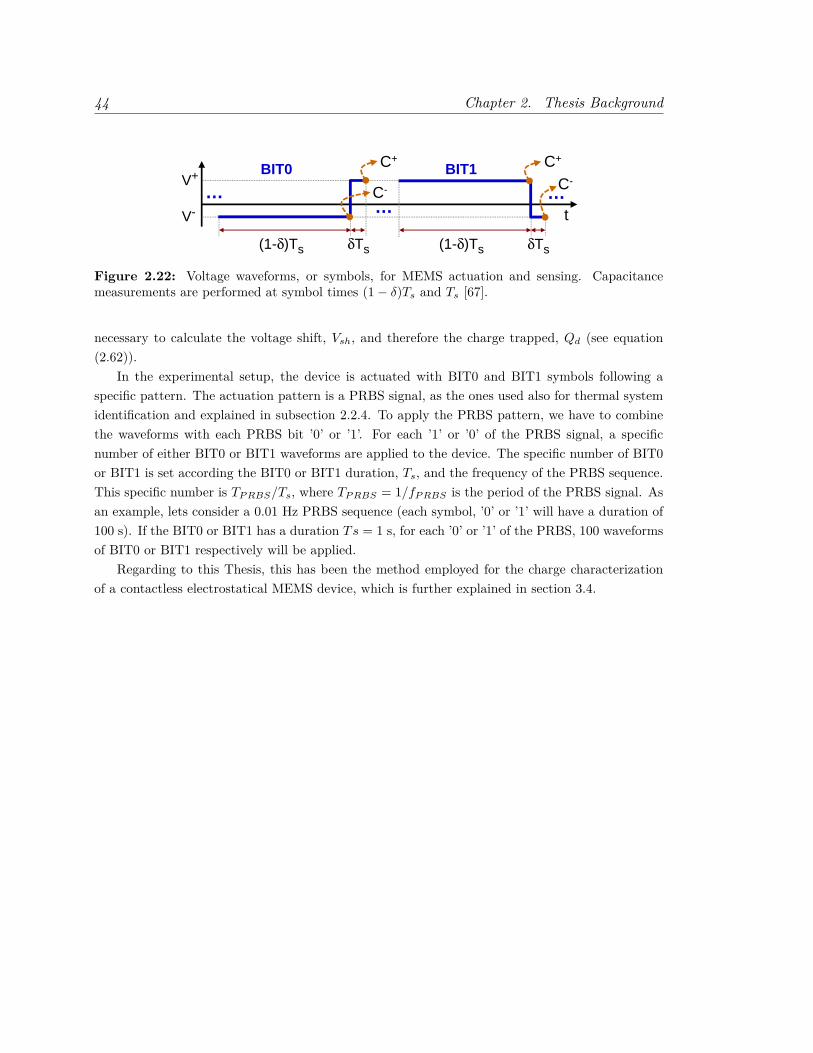
44 Chapter 2. Thesis Background
V+
V-
(1-δ)Ts
……
δTs
…BIT0 BIT1C+
C-
(1-δ)Ts δTs
C-
C+
t
Figure 2.22: Voltage waveforms, or symbols, for MEMS actuation and sensing. Capacitancemeasurements are performed at symbol times (1− δ)Ts and Ts [67].
necessary to calculate the voltage shift, Vsh, and therefore the charge trapped, Qd (see equation(2.62)).
In the experimental setup, the device is actuated with BIT0 and BIT1 symbols following aspecific pattern. The actuation pattern is a PRBS signal, as the ones used also for thermal systemidentification and explained in subsection 2.2.4. To apply the PRBS pattern, we have to combinethe waveforms with each PRBS bit ’0’ or ’1’. For each ’1’ or ’0’ of the PRBS signal, a specificnumber of either BIT0 or BIT1 waveforms are applied to the device. The specific number of BIT0or BIT1 is set according the BIT0 or BIT1 duration, Ts, and the frequency of the PRBS sequence.This specific number is TPRBS/Ts, where TPRBS = 1/fPRBS is the period of the PRBS signal. Asan example, lets consider a 0.01 Hz PRBS sequence (each symbol, ’0’ or ’1’ will have a duration of100 s). If the BIT0 or BIT1 has a duration Ts = 1 s, for each ’0’ or ’1’ of the PRBS, 100 waveformsof BIT0 or BIT1 respectively will be applied.
Regarding to this Thesis, this has been the method employed for the charge characterizationof a contactless electrostatical MEMS device, which is further explained in section 3.4.

Bibliography 45
Bibliography
[1] L. Gottesdiener. Hot wire anemometry in rarefied gas flow. Journal of Physics E: ScientificInstruments, 13(9):908, 1980.
[2] C. Holstein-Rathlou, J. Merrison, J. J. Iversen, A. B. Jakobsen, R. Nicolajsen, P. Nørnberg,K. Rasmussen, A. Merlone, G. Lopardo, T. Hudson, D. Banfield, and G. Portyankina. Anenvironmental wind tunnel facility for testing meteorological sensor systems. Journal ofAtmospheric and Oceanic Technology, 31(2):447–457, 2014.
[3] Peter A. Taylor, David C. Catling, Mike Daly, Cameron S. Dickinson, Haraldur P. Gunnlaugs-son, Ari-Matti Harri, and Carlos F. Lange. Temperature, pressure, and wind instrumentationin the phoenix meteorological package. Journal of Geophysical Research: Planets, 113(E3),2008. ISSN 2156-2202.
[4] Y. Zhu, B. Chen, M. Qin, and Q. A. Huang. 2-d micromachined thermal wind sensors: Areview. IEEE Internet of Things Journal, 1(3):216–232, June 2014. ISSN 2327-4662.
[5] M. Domínguez, V. Jiménez, J. Ricart, L. Kowalski, J. Torres, S. Navarro, J. Romeral, andL. Castañer. A hot film anemometer for the martian atmosphere. Planetary and SpaceScience, 56(8):1169 – 1179, 2008. ISSN 0032-0633.
[6] T. E. Chamberlain, H. L. Cole, R. G. Dutton, G. C. Greene, and J. E. Tillman. Atmop-spheric measurements on mars: the viking meteorology experiment. Bulletin of the AmericanMeteorological Society, 57(9):1094–1104, 1976.
[7] S. L. Hess, R. M. Henry, C. B. Leovy, J. A. Ryan, and J. E. Tillman. Meteorological resultsfrom the surface of mars: Viking 1 and 2. Journal of Geophysical Research, 82(28):4559–4574,1977. ISSN 2156-2202.
[8] James R. Murphy, Conway B. Leovy, and James E. Tillman. Observations of martian surfacewinds at the viking lander 1 site. Journal of Geophysical Research: Solid Earth, 95(B9):14555–14576, 1990. ISSN 2156-2202.
[9] NASA. Mars pathfinder web site, . URL https://mars.nasa.gov/MPF/mpf/sci_desc.html#ATMO.
[10] Alvin Seiff, James E. Tillman, James R. Murphy, John T. Schofield, David Crisp, Jeffrey R.Barnes, Clayton LaBaw, Colin Mahoney, John D. Mihalov, Gregory R. Wilson, and RobertHaberle. The atmosphere structure and meteorology instrument on the mars pathfinderlander. Journal of Geophysical Research: Planets, 102(E2):4045–4056, 1997. ISSN 2156-2202.

46 Bibliography
[11] J. T. Schofield, J. R. Barnes, D. Crisp, R. M. Haberle, S. Larsen, J. A. Magalhães, J. R.Murphy, A. Seiff, and G. Wilson. The mars pathfinder atmospheric structure investiga-tion/meteorology (asi/met) experiment. Science, 278(5344):1752–1758, 1997. ISSN 00368075,10959203.
[12] J. Gómez-Elvira, C. Armiens, L. Castañer, M. Domínguez, M. Genzer, F. Gómez, R. Haberle,A.-M. Harri, V. Jiménez, H. Kahanpää, L. Kowalski, A. Lepinette, J. Martín, J. Martínez-Frías, I. McEwan, L. Mora, J. Moreno, S. Navarro, M. A. de Pablo, V. Peinado, A. Peña,J. Polkko, M. Ramos, N. O. Renno, J. Ricart, M. Richardson, J. Rodríguez-Manfredi,J. Romeral, E. Sebastián, J. Serrano, M. de la Torre Juárez, J. Torres, F. Torrero, R. Urquí,L. Vázquez, T. Velasco, J. Verdasca, M.-P. Zorzano, and J. Martín-Torres. Rems: The envi-ronmental sensor suite for the mars science laboratory rover. Space Science Reviews, 170(1):583–640, 2012. ISSN 1572-9672.
[13] S. Rafkin, J. Pla-Garcia, C. Newman, V. Hamilton, J. Martin-Torres, M. PazZorzano, H. Ka-hanpaa, and E. Sebastian. The meteorology of gale crater determined from msl rems dataand mesoscale modeling. In Proc. 8th Int. Conf. Mars, pages 1–2, 2014.
[14] CAB (CSIC-INTA). Rover environmental monitoring station web site. URL https://cab.inta-csic.es/rems/intrument-description/wind-sensor/.
[15] NASA. Mars science laboratory web site, . URL https://mars.nasa.gov/msl/mission/instruments/environsensors/rems/.
[16] C. Bettanini, F. Esposito, S. Debei, C. Molfese, G. Colombatti, A. Aboudan, J. R. Bru-cato, F. Cortecchia, G. Di Achille, G. P. Guizzo, E. Friso, F. Ferri, L. Marty, V. Mennella,R. Molinaro, P. Schipani, S. Silvestro, R. Mugnuolo, S. Pirrotta, E. Marchetti, A. M. Harri,F. Montmessin, C. Wilson, I. A. Rodríguez, S. Abbaki, V. Apestigue, G. Bellucci, J. J. Berthe-lier, S. B. Calcutt, F. Forget, M. Genzer, P. Gilbert, H. Haukka, J. J. Jiménez, S. Jiménez,J. L. Josset, O. Karatekin, G. Landis, R. Lorenz, J. Martinez, D. Möhlmann, D. Moirin,E. Palomba, M. Pateli, J. P. Pommereau, C. I. Popa, S. Rafkin, P. Rannou, N. O. Renno,W. Schmidt, F. Simoes, A. Spiga, F. Valero, L. Vázquez, F. Vivat, and O. Witasse. Thedreams experiment flown on the exomars 2016 mission for the study of martian environ-ment during the dust storm season. In 2017 IEEE International Workshop on Metrology forAeroSpace (MetroAeroSpace), pages 249–255, June 2017.
[17] M.C. Towner, M.R. Patel, T.J. Ringrose, J.C. Zarnecki, D. Pullan, M.R. Sims, S. Haapanala,A.-M. Harri, J. Polkko, C.F. Wilson, A.P. Zent, R.C. Quinn, F.J. Grunthaner, M.H. Hecht,and J.R.C. Garry. The beagle 2 environmental sensors: science goals and instrument descrip-tion. Planetary and Space Science, 52(13):1141 – 1156, 2004. ISSN 0032-0633.
[18] Lukasz Kowalski. Contribution to Advanced Hot Wire Wind Sensing. PhD thesis, UniversitatPolitécnica de Catalunya, 2016.

Bibliography 47
[19] L. Kowalski, M. T. Atienza, S. Gorreta, V. Jiménez, M. Domínguez-Pumar, S. Silvestre, andL. M. Castañer. Spherical wind sensor for the atmosphere of mars. IEEE Sensors Journal,16(7):1887–1897, April 2016. ISSN 1530-437X.
[20] NASA. Insight mission web site, . URL https://insight.jpl.nasa.gov/home.cfm.
[21] NASA. Mars environmental dynamics analyzer web site, . URL https://mars.nasa.gov/mars2020/mission/instruments/meda/.
[22] M.N. Sabry, W. Fikry, Kh. Abdel Salam, M.M. Awad, and A.E. Nasser. A lumped transientthermal model for self-heating in mosfets. Microelectronics Journal, 32(10):847 – 853, 2001.ISSN 0026-2692.
[23] M. N. Sabry. Compact thermal models for electronic systems. IEEE Transactions on Com-ponents and Packaging Technologies, 26(1):179–185, March 2003. ISSN 1521-3331.
[24] M. Rencz and V. Szekely. Dynamic thermal multiport modeling of ic packages. IEEE Transac-tions on Components and Packaging Technologies, 24(4):596–604, Dec 2001. ISSN 1521-3331.
[25] S. Y. Lee, A. G. Pfaelzer, and J. D. van Wyk. Comparison of different designs of a 42-v/14-v dc/dc converter regarding losses and thermal aspects. IEEE Transactions on IndustryApplications, 43(2):520–530, March 2007. ISSN 0093-9994.
[26] Guifang Guo, Bo Long, Bo Cheng, Shiqiong Zhou, Peng Xu, and Binggang Cao. Three-dimensional thermal finite element modeling of lithium-ion battery in thermal abuse appli-cation. Journal of Power Sources, 195(8):2393 – 2398, 2010. ISSN 0378-7753.
[27] Dong Hyup Jeon. Numerical modeling of lithium ion battery for predicting thermal behaviorin a cylindrical cell. Current Applied Physics, 14(2):196 – 205, 2014. ISSN 1567-1739.
[28] P. L. Evans, A. Castellazzi, and C. M. Johnson. Automated fast extraction of compactthermal models for power electronic modules. IEEE Transactions on Power Electronics, 28(10):4791–4802, Oct 2013. ISSN 0885-8993.
[29] S. Gao, Z. Yi, Y. Ye, Q. A. Huang, and M. Qin. Design and optimization of thermal-mechanical reliability of a tsv 3d packaged thermal wind sensor. In 2017 18th InternationalConference on Electronic Packaging Technology (ICEPT), pages 584–587, Aug 2017.
[30] Jonathan N. Davidson. Advanced thermal modelling and management techniques to improvepower density in next generation power electronics. PhD thesis, The University of Sheffield,2015.
[31] R. Wrobel, N. McNeill, and P. H. Mellor. Performance analysis and thermal modeling of ahigh-energy-density prebiased inductor. IEEE Transactions on Industrial Electronics, 57(1):201–208, Jan 2010. ISSN 0278-0046.

48 Bibliography
[32] B. H. Lee, K. S. Kim, J. W. Jung, J. P. Hong, and Y. K. Kim. Temperature estimation ofipmsm using thermal equivalent circuit. IEEE Transactions on Magnetics, 48(11):2949–2952,Nov 2012. ISSN 0018-9464.
[33] K. Murthy and R. Bedford. Transformation between foster and cauer equivalent networks.IEEE Transactions on Circuits and Systems, 25(4):238–239, April 1978. ISSN 0098-4094.
[34] K. Ma, N. He, M. Liserre, and F. Blaabjerg. Frequency-domain thermal modeling and char-acterization of power semiconductor devices. IEEE Transactions on Power Electronics, 31(10):7183–7193, Oct 2016. ISSN 0885-8993.
[35] J. N. Davidson, D. A. Stone, M. P. Foster, and C. R. Gould. Prediction of device temperaturesin an electric vehicle battery charger system by analysis of device thermal cross-coupling. In2013 15th European Conference on Power Electronics and Applications (EPE), pages 1–9,Sept 2013.
[36] J. N. Davidson, D. A. Stone, and M. P. Foster. Real-time prediction of power electronic devicetemperatures using prbs-generated frequency-domain thermal cross coupling characteristics.IEEE Transactions on Power Electronics, 30(6):2950–2961, June 2015. ISSN 0885-8993.
[37] X. Hu, S. Lin, S. Stanton, and W. Lian. A foster network thermal model for hev/ev batterymodeling. IEEE Transactions on Industry Applications, 47(4):1692–1699, July 2011. ISSN0093-9994.
[38] T. Bruckner and S. Bernet. Estimation and measurement of junction temperatures in athree-level voltage source converter. IEEE Transactions on Power Electronics, 22(1):3–12,Jan 2007. ISSN 0885-8993.
[39] K. Gorecki and J. Zarebski. Nonlinear compact thermal model of power semiconductordevices. IEEE Transactions on Components and Packaging Technologies, 33(3):643–647,Sept 2010. ISSN 1521-3331.
[40] J. N. Davidson, D. A. Stone, and M. P. Foster. Required cauer network order for modellingof thermal transfer impedance. Electronics Letters, 50(4):260–262, February 2014. ISSN0013-5194.
[41] A. Bryant, N. A. Parker-Allotey, D. Hamilton, I. Swan, P. A. Mawby, T. Ueta, T. Nishijima,and K. Hamada. A fast loss and temperature simulation method for power converters, parti: Electrothermal modeling and validation. IEEE Transactions on Power Electronics, 27(1):248–257, Jan 2012. ISSN 0885-8993.
[42] I. Swan, A. Bryant, P. A. Mawby, T. Ueta, T. Nishijima, and K. Hamada. A fast loss andtemperature simulation method for power converters, part ii: 3-d thermal model of powermodule. IEEE Transactions on Power Electronics, 27(1):258–268, Jan 2012. ISSN 0885-8993.

Bibliography 49
[43] P. M. Igic, P. A. Mawby, M. S. Towers, and S. Batcup. New physically-based pin diodecompact model for circuit modelling applications. IEE Proceedings - Circuits, Devices andSystems, 149(4):257–263, Aug 2002. ISSN 1350-2409.
[44] J. N. Davidson, D. A. Stone, M. P. Foster, and D. T. Gladwin. Improved bandwidth and noiseresilience in thermal impedance spectroscopy by mixing prbs signals. IEEE Transactions onPower Electronics, 29(9):4817–4828, Sept 2014. ISSN 0885-8993.
[45] J. D. Gabano, T. Poinot, and H. Kanoun. Identification of a thermal system using continuouslinear parameter-varying fractional modelling. IET Control Theory Applications, 5(7):889–899, May 2011. ISSN 1751-8644.
[46] W.D.T. Davies. System Identification for Self-adaptive Control. Davies. Wiley-Interscience,1970.
[47] A.J. Saavedra-Montes, J.M. Ramirez-Scarpetta, C.A. Ramos-Paja, and O.P. Malik. Identifi-cation of excitation systems with the generator online. Electric Power Systems Research, 87(Supplement C):1 – 9, 2012. ISSN 0378-7796.
[48] M. Singh, M. Sakare, and S. Gupta. Testing of high-speed dacs using prbs generation withalternate–bit–tapping. In 2011 Design, Automation Test in Europe, pages 1–6, March 2011.
[49] A.J. Fairweather, M.P. Foster, and D.A. Stone. Battery parameter identification with pseudorandom binary sequence excitation (prbs). Journal of Power Sources, 196(22):9398 – 9406,2011. ISSN 0378-7753.
[50] J. N. Davidson, D. A. Stone, and M. P. Foster. Real-time temperature monitoring andcontrol for power electronic systems under variable active cooling by characterisation of devicethermal transfer impedance. In 7th IET International Conference on Power Electronics,Machines and Drives (PEMD 2014), pages 1–6, April 2014.
[51] G. Montseny, J. Audounet, and B. Mbodje. Optimal models of fractional integrators andapplication to systems with fading memory. In Proceedings of IEEE Systems Man and Cy-bernetics Conference - SMC, pages 65–70 vol.5, Oct 1993.
[52] Montseny, Gérard. Diffusive representation of pseudo-differential time-operators. ESAIM:Proc., 5:159–175, 1998.
[53] C. Casenave and G. Montseny. Introduction to diffusive representation. IFAC ProceedingsVolumes, 43(21):370 – 377, 2010. ISSN 1474-6670. 4th IFAC Symposium on System Structureand Control.
[54] Gerard Montseny. Representation diffusive. Lavoisier, 2005.

50 Bibliography
[55] Jacques Audounet, Vincent Giovangigli, and Jean-Michel Roquejoffre. A threshold phe-nomenon in the propagation of a point source initiated flame. Physica D: Nonlinear Phenom-ena, 121(3):295 – 316, 1998. ISSN 0167-2789.
[56] F. Levernhe, G. Montseny, and J. Audounet. Markovian diffusive representation of 1/f alpha;noises and application to fractional stochastic differential models. IEEE Transactions onSignal Processing, 49(2):414–423, Feb 2001. ISSN 1053-587X.
[57] David Levadoux and Gérard Montseny. Diffusive Realization of the Impedance Operator onCircular Boundary for 2D Wave Equation, pages 136–141. Springer Berlin Heidelberg, Berlin,Heidelberg, 2003. ISBN 978-3-642-55856-6.
[58] J. Solhusvik, F. Lavernhe, G. Montseny, and J. A. Farre. A new low-noise ccd signal acqui-sition method based on a commutable band-pass filter. IEEE Transactions on Circuits andSystems II: Analog and Digital Signal Processing, 44(3):164–173, Mar 1997. ISSN 1057-7130.
[59] L. Laudebat, P. Bidan, and G. Montseny. Modeling and optimal identification of pseudod-ifferential electrical dynamics by means of diffusive representation-part i: modeling. IEEETransactions on Circuits and Systems I: Regular Papers, 51(9):1801–1813, Sept 2004. ISSN1549-8328.
[60] Lionel Laudebat. Modélisation et identification sous repreésentation diffusive de comporte-ments dynamiques non rationnels en génie électrique. PhD thesis, Universite Toulouse III -Paul Sabatier, 2003.
[61] Emilie Blanc, Guillaume Chiavassa, and Bruno Lombard. A time-domain numerical modelingof two-dimensional wave propagation in porous media with frequency-dependent dynamicpermeability. The Journal of the Acoustical Society of America, 134(6):4610–4623, 2013.
[62] B. Allard, X. Jorda, P. Bidan, A. Rumeau, H. Morel, X. Perpina, M. Vellvehi, and S. M’Rad.Reduced-order thermal behavioral model based on diffusive representation. IEEE Transac-tions on Power Electronics, 24(12):2833–2846, Dec 2009. ISSN 0885-8993.
[63] K. B. Smida, P. Bidan, T. Lebey, F. B. Ammar, and M. Elleuch. Identification and time-domain simulation of the association inverter–cable–asynchronous machine using diffusiverepresentation. IEEE Transactions on Industrial Electronics, 56(1):257–265, Jan 2009. ISSN0278-0046.
[64] S. M’Rad, B. Allard, H. Morel, A. Ammous, and N. Masmoudi. Analytic thermal modelling ofpower electronic components: The diffusive representation. In 4th International Conferenceon Integrated Power Systems, pages 1–6, June 2006.
[65] S. Mrad, P. Lefranc, P. Dessante, P. Chiozzi, G. Blondel, M. Fakes, and P. Masson. A compacttransient electrothermal model for integrated power systems: Automotive application. In 200935th Annual Conference of IEEE Industrial Electronics, pages 3755–3760, Nov 2009.
Bibliography 51
[66] C. Restrepo, G. Garcia, J. Calvente, R. Giral, and L. Martínez-Salamero. Static and dynamiccurrent – voltage modeling of a proton exchange membrane fuel cell using an input – outputdiffusive approach. IEEE Transactions on Industrial Electronics, 63(2):1003–1015, Feb 2016.ISSN 0278-0046.
[67] M. T. Atienza, S. Gorreta, J. Pons-Nin, and M. Dominguez-Pumar. Characterization ofdielectric charging in mems using diffusive representation. IEEE Transactions on IndustrialElectronics, 64(2):1529–1533, Feb 2017. ISSN 0278-0046.
[68] G. Montseny. Simple approach to approximation and dynamical realization of pseudodiffer-ential time operators such as fractional ones. IEEE Transactions on Circuits and Systems II:Express Briefs, 51(11):613–618, Nov 2004. ISSN 1549-7747.
[69] Kenneth S. Cole and Robert H. Cole. Dispersion and absorption in dielectrics i. alternatingcurrent characteristics. The Journal of Chemical Physics, 9(4):341–351, 1941.
[70] Kenneth S. Cole and Robert H. Cole. Dispersion and absorption in dielectrics ii. direct currentcharacteristics. The Journal of Chemical Physics, 10(2):98–105, 1942.
[71] Yuri P. Kalmykov, William T. Coffey, Derrick S. F. Crothers, and Sergey V. Titov. Micro-scopic models for dielectric relaxation in disordered systems. Phys. Rev. E, 70:041103, Oct2004.
[72] Z. Lin. On the fdtd formulations for biological tissues with cole–cole dispersion. IEEEMicrowave and Wireless Components Letters, 20(5):244–246, May 2010. ISSN 1531-1309.
[73] B. Maundy and A. S. Elwakil. Extracting single dispersion cole–cole impedance model pa-rameters using an integrator setup. Analog Integrated Circuits and Signal Processing, 71(1):107–110, Apr 2012. ISSN 1573-1979.
[74] V. Utkin, J. Guldner, and M. Shijun. Sliding Mode Control in Electro-mechanical Systems.Automation and Control Engineering. Taylor & Francis, 1999. ISBN 9780748401161.
[75] Shuanghe Yu, Xinghuo Yu, Bijan Shirinzadeh, and Zhihong Man. Continuous finite-timecontrol for robotic manipulators with terminal sliding mode. Automatica, 41(11):1957 –1964, 2005. ISSN 0005-1098.
[76] Yong Feng, Xinghuo Yu, and Zhihong Man. Non-singular terminal sliding mode control ofrigid manipulators. Automatica, 38(12):2159 – 2167, 2002. ISSN 0005-1098.
[77] Oscar Camacho and Carlos A. Smith. Sliding mode control: an approach to regulate nonlinearchemical processes. ISA Transactions, 39(2):205 – 218, 2000. ISSN 0019-0578.
[78] Steven R Norsworthy, Richard Schreier, Gabor C Temes, et al. Delta-sigma data converters:theory, design, and simulation, volume 97. IEEE press New York, 1996.

52 Bibliography
[79] S. Gorreta, J. Pons-Nin, E. Blokhina, O. Feely, and M. Domínguez-Pumar. Delta-sigmacontrol of dielectric charge for contactless capacitive mems. Journal of MicroelectromechanicalSystems, 23(4):829–841, Aug 2014. ISSN 1057-7157.
[80] M. Dominguez-Pumar, S. Gorreta, and J. Pons-Nin. Sliding-mode analysis of the dynamicsof sigma-delta controls of dielectric charging. IEEE Transactions on Industrial Electronics,63(4):2320–2329, April 2016. ISSN 0278-0046.
[81] Hebertt Sira-Ramírez. Sliding Mode Control. The Delta-Sigma Modulation Approach.Birkhäuser Basel, 2015.
[82] Y. Shtessel, C. Edwards, L. Fridman, and A. Levant. Sliding Mode Control and Observation.Control Engineering. Springer New York, 2013. ISBN 9780817648930.
[83] Vadim I. Utkin. Sliding Modes in Control and Optimization. Springer-Verlag Berlin Heidel-berg, 1992.
[84] J. Yuan and B. Shi Y. Zhang, J. Liu. Sliding mode control of vibration in single-degree-of-freedom fractional oscillators. Journal of Dynamic Systems, Measurement, and Control,pages 114503–114509, July 2017. ISSN 0278-0046.
[85] Maamar Bettayeb and Said Djennoune. Design of sliding mode controllers for nonlinearfractional-order systems via diffusive representation. Nonlinear Dynamics, 84(2):593–605,Apr 2016. ISSN 1573-269X.
[86] E. Blokhina, S. Gorreta, D. Lopez, D. Molinero, O. Feely, J. Pons-Nin, and M. Dominguez-Pumar. Dielectric charge control in electrostatic mems positioners/varactors. Journal ofMicroelectromechanical Systems, 21(3):559–573, June 2012. ISSN 1057-7157.
[87] R. W. Herfst, P. G. Steeneken, H. G. A. Huizing, and J. Schmitz. Center-shift method forthe characterization of dielectric charging in rf mems capacitive switches. IEEE Transactionson Semiconductor Manufacturing, 21(2):148–153, May 2008. ISSN 0894-6507.
[88] R. W. Herfst, H. G. A. Huizing, P. G. Steeneken, and J. Schmitz. Characterization ofdielectric charging in rf mems capacitive switches. In 2006 IEEE International Conferenceon Microelectronic Test Structures, pages 133–136, March 2006.
[89] G. Papaioannou, M.N. Exarchos, V. Theonas, G. Wang, and J. Papapolymerou. Temperaturestudy of the dielectric polarization effects of capacitive RF MEMS switches. IEEE JMTT,53:3467–3473, 2005.
[90] Z. Olszewski, R. Duane, and C. O’Mahony. Effect of environment humidity on the C-V char-acteristics of RF MEMS capacitive switch. In 9th Int. Symp. on RF MEMS and Microsystems(MEMSWAVE), 29 June - 4 July 2008.

Bibliography 53
[91] S.M. Sze and K.K. Ng. Physics of Semiconductor Devices. Third Edition. Wiley, 2007.
[92] M. Razeghi. Fundamentals of Solid State Engineering. Sec. Edition. Springer, 2006.
[93] Andreas Gehring and Siegfried Selberherr. Modeling of tunneling current and gate dielectricreliability for nonvolatile memory devices. Device and Materials Reliability, IEEE Trans. on,4(3):306–319, 2004.
[94] Ankit Jain, Sambit Palit, and Muhammad Ashraful Alam. A physics-based predictive mod-eling framework for dielectric charging and creep in RF MEMS capacitive switches and var-actors. Microelectromechanical Systems, Journal of, 21(2):420–430, 2012.
[95] A. Koszewski, F. Souchon, Ch. Dieppedale, D. Bloch, and T. Ouisse. Physical model ofdielectric charging in MEMS. Journal of Micromechanics and Microengineering, 23(4):045019,2013.
[96] S. Gorreta, J. Pons-Nin, M. Dominguez-Pumar, E. Blokhina, and O. Feely. Characterizationmethod of the dynamics of the trapped charge in contactless capacitive mems. In 2014Symposium on Design, Test, Integration and Packaging of MEMS/MOEMS (DTIP), pages1–6, April 2014.
[97] Manuel Dominguez-Pumar, Sergi Gorreta, Joan Pons-Nin, Elena Blokhina, PanagiotisGiounanlis, and Orla Feely. Real-time characterization of dielectric charging in contactlesscapacitive mems. Analog Integrated Circuits and Signal Processing, 82(3):559–569, Mar 2015.ISSN 1573-1979.
[98] Sergi Gorreta. Dielectric charge control in contactless capacitive MEMS. PhD thesis, Uni-versitat Politécnica de Catalunya, 2017.
[99] R.W. Herfst, P.G. Steeneken, and J. Schmitz. Time and voltage dependence of dielectriccharging in RF MEMS capacitive switches. In IEEE 45th Annual Int. Reliability PhysicsSymp., Phoenix, pages 417–421, 2007.
[100] Mohamed Matmat, Fabio Coccetti, Antoine Marty, Robert Plana, Christophe Escriba, Jean-Yves Fourniols, and Daniel Esteve. Capacitive rf mems analytical predictive reliability andlifetime characterization. Microelectronics Reliability, 49(9):1304 – 1308, 2009. ISSN 0026-2714. 20th European Symposium on the Reliability of Electron Devices, Failure Physics andAnalysis.
[101] X. Yuan, J.C.M. Hwang, D. Forehand, and C.L. Goldsmith. Modeling and characterizationof dielectric-charging effects in RF MEMS capacitive switches. In Digest of IEEE MTT-S2005 Microwave Symposium Digest, pages 753–756, 2005.
[102] Xiaobin Yuan, Zhen Peng, J. C. M. Hwang, D. Forehand, and C. L. Goldsmith. A transientspice model for dielectric-charging effects in rf mems capacitive switches. IEEE Transactionson Electron Devices, 53(10):2640–2648, Oct 2006. ISSN 0018-9383.

54 Bibliography
[103] Z. Peng, X. Yuan, J. C. M. Hwang, D. I. Forehand, and C. L. Goldsmith. Superpositionmodel for dielectric charging of RF MEMS capacitive switches under bipolar control-voltagewaveforms. IEEE JMTT, 55:2911–2918, 2007.
[104] M. Matmat, K. Koukos, F. Coccetti, T. Idda, A. Marty, C. Escriba, J-Y. Fourniols, and D. Es-teve. Life expectancy and characterization of capacitive RF MEMS switches. MicroelectronicsReliability, 50:1692–1696, 2010.
[105] U. Zaghloul, G. Papaioannou, F. Coccetti, P. Pons, and R. Plana. Dielectric charging insilicon nitride films for mems capacitive switches: Effect of film thickness and depositionconditions. Microelectronics Reliability, 49(9):1309 – 1314, 2009. ISSN 0026-2714. 20thEuropean Symposium on the Reliability of Electron Devices, Failure Physics and Analysis.
[106] U Zaghloul, G J Papaioannou, F Coccetti, P Pons, and R Plana. A systematic reliabil-ity investigation of the dielectric charging process in electrostatically actuated mems basedon kelvin probe force microscopy. Journal of Micromechanics and Microengineering, 20(6):064016, 2010.
[107] R. W. Herfst, P. G. Steeneken, J. Schmitz, A. J. G. Mank, and M. van Gils. Kelvin probestudy of laterally inhomogeneous dielectric charging and charge diffusion in rf mems capacitiveswitches. In 2008 IEEE International Reliability Physics Symposium, pages 492–495, April2008.
[108] Hiroaki Hara and Yoshiyasu Tamura. Dynamical process of complex systems and fractionaldifferential equations. Central European Journal of Physics, 11(10):1238–1245, 2013. ISSN1644-3608.
[109] M. Kouteoureli and G. Papaioannou. The discharge current through the dielectric film inMEMS capacitive switches. In European Microwave Integrated Circuits Conference (EuMIC),pages 450–453, Oct 2011.
[110] S. Gorreta, J. Pons-Nin, E. Blokhina, and M. Dominguez. A second-order delta-sigma con-trol of dielectric charge for contactless capacitive mems. Journal of MicroelectromechanicalSystems, 24(2):259–261, April 2015. ISSN 1057-7157.
[111] S. Gorreta, J. Pons-Nin, and M. Dominguez-Pumar. Simultaneous control of dielectric chargeand device capacitance in electrostatic mems. Journal of Microelectromechanical Systems, 24(6):1684–1686, Dec 2015. ISSN 1057-7157.

Chapter 3
Compendium of Publications
This chapter describes the most important part of the research work carried out during the Thesis,
in the form of a compendium of publications. The list of publications together with the abstracts
is presented first, and after the complete publications in postprint format is presented.
ATTENTION¡¡
For copyright reasons publications must be consulted on the publisher's
website indicated in the grey box
Published:
1. Heat Flow Dynamics in Thermal Systems Described by Diffusive Representation
on page 59.
Abstract—The objective of this paper is to analyze the dynamics of heat flow in thermal
structures working under constant temperature operation. This analysis is made using the
tools of sliding mode controllers. The theory is developed considering that the thermal
system can be described using diffusive representation. The experimental corroboration has
been made with a prototype of a wind sensor for Mars atmosphere being controlled by a
thermal sigma-delta modulator. This sensor structure allows to analyze the time-varying
case experimentally since changes in wind conditions imply changes in the corresponding
thermal models. The diffusive symbols of the experimental structures have been obtained
from open-loop measurements in which pseudorandom binary sequences of heat are injected in
the sensor. With the proposed approach, it is possible to predict heat flux transientwaveforms
in systems described by any arbitrary number of poles. This allows for the first time the
analysis of lumped and distributed systems without any limitation on the number of poles
describing it.
Published in IEEE - Transactions on Industrial Electronics, vol. 64, no. 1, pp. 664–673,
Jan. 2017.
http://ieeexplore.ieee.org/document/7558240/
2. Spherical Wind Sensor for the Atmosphere of Mars on page 69.
Abstract—A novel wind speed and direction sensor designed for the atmosphere of Mars
is described. It is based on a spherical shell divided into four triangular sectors according
55

56 Chapter 3. Compendium of Publications
to the central projection of tetrahedron onto the surface of the unit sphere. Each sector
is individually controlled to be heated above the ambient temperature independently of the
wind velocity and incidence angle. A convection heat rate model of four hot spherical triangles
under forced wind has been built with finite element method thermal–fluidic simulations. The
angular sensitivity of the tetrahedral sphere structure has been theoretically determined and
compared with the tessellation of the sphere by four biangles. A 9-mm-diameter prototype
has been assembled using 3-D printing of the spherical shell housing in the interior commercial
platinum resistors connected to an extension of a custom design printed board. Measurements
in Martianlike atmosphere demonstrate sensor responsiveness to the flow in the velocity range
1–13 m/s at 10-mBar CO2 pressure. Numerical modelization of the sensor behavior allows to
devise an inverse algorithm to retrieve the wind direction data from the raw measurements
of the power delivered to each spherical sector. The functionality of the inverse algorithm is
also demonstrated.
Published in IEEE - Sensors Journal, vol. 16, no. 7, pp. 1887–1897, Apr. 2016.
http://ieeexplore.ieee.org/document/7358056/
3. Sliding mode analysis applied to improve the dynamical response of a spherical
3D wind sensor for Mars atmosphere on page 81.
Abstract—The objective of this paper is to show how the structure of a thermal wind
anemometer can be tuned to ensure a fast response when the sensor works in closed loop
configuration (constant temperature operation). If the thermal filter associated to the sensor
structure has only one significative time constant, the resulting system time response, work-
ing in closed loop, is enhanced beyond the natural limit imposed by its own thermal circuit.
This effect is theoretically explained using the theory of sliding mode controllers. Experi-
mental corroboration is presented by comparing the results obtained with two prototypes of
a spherical wind sensor for Mars atmosphere. It will be shown that in case of having only
one significant time constant, the time response in closed loop is much faster than the value
associated with that time constant. It will be experimentally shown that this effect is lost
when the thermal filter has more than one significant time constant. Diffusive representation
is used to obtain arbitrary-order models of the thermal structures of the sensors.
Published in Sensors And Actuators A: Physical, vol. 267, pp. 342–350, Sep. 2017.
https://www.sciencedirect.com/science/article/pii/S0924424717308828
4. Characterization of Dielectric Charging in MEMS Using Diffusive Representa-
tion on page 91.
Abstract—This paper introduces diffusive representation as a novel approach to characterize
the dynamics of charge trapped in the dielectric layers of microelectromechanical systems.
Diffusive representation provides a computationally efficient method to achieve an arbitrary
order statespace model of the charging dynamics. This approach is particularly well suited
to analyze the dynamics of the dielectric charge under nontrivial controls, as in the case
of sliding mode controllers. The diffusive symbol of the experimental structure has been
obtained from open-loop measurements, in which the pseudo random binary sequences are
applied to the device. The obtained model exhibits good agreement with the experimental

57
data and also allows us to model the behavior of the charge dynamics under excitation with
arbitrary binary signals.
Published in IEEE - Transactions on Industrial Electronics, vol. 64, no. 2, pp. 1529–1533,
Feb. 2017.
http://ieeexplore.ieee.org/document/7574316/

Chapter 4
Other Thesis-related Work
This chapter includes a report of the research work done in the analysis of the thermal dynamicsof the egineering model prototype of the REMS wind sensor. This work was realized in the Centrode Astrobiologia (CAB, CSIC-INTA) facilities in Madrid, during a three months stay along 2017.The results presented in this report are part of a journal paper that is actually submitted andunder review. Although it is not possible to include it in the compendium of publications, it is animportant part of the work developed during the research work of this Thesis.
The abstract of the submitted journal paper and the report containing a summary of the resultsobtained are presented.
Works:1. Thermal Dynamics Modeling of a 3D Wind Sensor Based on Hot Thin Film
Anemometry.
Abstract—The objective of this paper is to obtain time-varying models of the thermal dynam-ics of a 3D hot thin film anemometer for Mars atmosphere. To this effect, a proof of conceptprototype of the REMS wind sensor on board the Curiosity rover has been used. The selfand cross-heating effects of the thermal structures have been characterized from open-loopmeasurements using Diffusive Representation. These models have been proven to be suitablein the analysis of the thermal dynamics of the sensor under constant temperature operationemploying the tools of Sliding Mode Controllers. This analysis allows to understand the longterm heat diffusion processes in the whole structure and how they may affect the raw outputsignals.
Under minor revision.
97


1 / 19
DYNAMICAL THERMAL MODELS FOR THE REMS-TWINS SENSOR
M.T. Atienza, L. Kowalski, M. Domínguez-Pumar
SUMMARY
- Dynamical model of self-heating and cross-heating of the silicon dice at different wind velocities. These models describe how the temperature of a part of the structure (a silicon die or the boom) depends on the heat dissipated in another part of the structure (in our case the silicon die). Diffusive representation models of self-heating in the dice and heating between dice (cross-heating) have been obtained. The self-heating models depend on wind velocity and they have been made for v=0 and ±7.5m/min. Self-heating (2.1.1): the models present significant exponentials at approximately 0.2-0.3Hz. The wind dependence can be parameterized as a variable amplitude of the pole at this frequency (higher velocity values, less amplitude). Cross-heating (2.1.2): a model at 0 wind velocity has been obtained in which the temperature evolution of each die is calculated as a function of the heat dissipated in another die. No relevant and consistent changes have been observed at different wind velocities, for the wind velocities tested. It has been observed symmetry in the models so that adjacent dice are heated in the same way, whereas the die in diagonal is heated differently and with much smaller amplitude. The most significant time constant in cross-heating is at 0.1Hz. The time evolution of the temperature in a die can be calculated as the superposition of the corresponding self-heating model and the associated cross-heating models. - Boom heating (2.2) A heating of 0.6-0.7ºC of the boom has been observed as a result of a 17ºC overheat of 4 silicon dice in one of the cards. A DR model has been obtained describing the temperature evolution in the boom as a result of the total power injected in the four dice of one card (the same current is applied to all dice at any given moment). Two main time constants have been found: 2x10⁻⁴ and 2x10⁻³ Hz (5000s and 500s respectively). -Prediction of the closed loop output from self-heating model (2.3.1 and 2.3.2) From the self-heating DR model of one die, a prediction of the output of the sigma-delta for this die, working in closed loop has been made. Wind velocity has been switched between ±7.5 m/min and 0. The analytically predicted results match the experimental results. (Figure 12).
- Comments:
- We think that an automatic control of the car in the CAB wind tunnel would be very useful.
- The influence of other heat sources (ASIC, sun radiation) on the boom temperature should be analyzed.
4.1. Report: Dynamical Thermal Models for the REMS-TWINS Sensor 99

2 / 19
- Fast changes in wind temperature have not been tested. - Appendices Many other additional experiments can be found in the Appendix
a) Corroboration of boom heating coming from dice. b) Dice heating coming from power dissipated in the boom resistor (!) both in open and
closed-loop measurements. Boom heating generates drift in the sigma-delta output of the dice.
1. INTRODUCTION The contents of this document are the final results obtained from the measurements done with the REMS wind sensor prototype in the wind tunnel facilities of CAB.
The boom of REMS wind sensor is composed of three PCBs placed 120º one from each other with four dice in each one. Each die has two resistors, one for heating and another for sensing, but due to practical reasons, we have only used the heating resistor both for heating and measuring the temperature. The wind tunnel of CAB facilities is a 5-meter linear wind tunnel. The operating method consists on a car on a rail that moves to a certain velocity. Having this into account, depending of the position of the boom the signal observed at a certain velocity will be different in straight movements from position 0 to position 5m than in reverse movement from 5m to position 0m. The velocities inside the tunnel can be adjusted from 6m/min to 30m/min, that makes the car do all the way from 0 to 5m in a range from 50s to 10s, which is a very short time, taking into account the expected time constants. That is why dynamical models are needed to fully characterize the thermal response of the whole sensor system, composed of silicon dice and boom. The boom is placed horizontally inside the tunnel. PCB1 is on top of the boom, while PCB2 and PCB3 have the normal at 120º from the top and are therefore looking downwards.
Figure 1: Boom mounted inside the tunnel Figure 2: Dice structure
100 Chapter 4. Other Thesis-related Work

3 / 19
In order to build finite order thermal models approximating the dynamical response of arbitrary thermal systems we have used Diffusive Representation (See Appendix 1). This mathematical tool allows generating arbitrary order models approximating experimental responses of diffusive systems, as in the case of thermal models. The main advantage of these models is that it is not necessary to make any a priori assumptions/approximations on the physical heat flows and temperature distributions of the structures and that it is possible to describe time variant systems such as the ones needed for wind sensing. Furthermore, it has been proved that with this tool it is possible to approximate even fractional order models (the ones associated typically with Partial Derivative Equations, PDEs), i.e., associated with heat diffusion on massive structures like the boom.
2. EXPERIMENTAL RESULTS Different experiments have been carried out intended to obtain the diffusive representation models that help understanding the thermal dynamics of the wind sensor of REMS.
2.1. AUTO AND CROSSED HEATING OF DICE Due to the proximity of the dice in the PCB, when heating one die, the rest of the dice in the PCB are affected. Therefore, when all the dice are working at the same time, the temperature of each die will depend on its self-heating current, and the current of the rest of the dice. In this section, we are going to obtain the thermal models that characterize the self-heating and cross-coupled effects. The diffusive representation equations are as follows: Auto – Heating
• Heating in die A. Temperature in die A. 𝑑𝑑𝛹𝛹𝑘𝑘
𝐴𝐴(𝑡𝑡)𝑑𝑑𝑡𝑡
= −𝜁𝜁𝑘𝑘𝛹𝛹𝑘𝑘𝐴𝐴(𝑡𝑡) + ɳ𝑘𝑘
(𝐴𝐴𝐴𝐴)𝑃𝑃𝐴𝐴(𝑡𝑡) 𝛹𝛹𝑘𝑘𝐴𝐴(0) = 0 𝑘𝑘 = 1 …𝐾𝐾
𝑇𝑇𝐴𝐴(𝑡𝑡) = 𝛹𝛹𝑘𝑘𝐴𝐴(𝑡𝑡)
𝑘𝑘
• Heating in die B. Temperature in die B.
𝑑𝑑𝛹𝛹𝑘𝑘
𝐵𝐵(𝑡𝑡)𝑑𝑑𝑡𝑡
(𝑡𝑡) = −𝜁𝜁𝑘𝑘𝛹𝛹𝑘𝑘𝐵𝐵(𝑡𝑡) + ɳ𝑘𝑘
(𝐵𝐵𝐵𝐵)𝑃𝑃𝐵𝐵(𝑡𝑡) 𝛹𝛹𝑘𝑘𝐵𝐵(0) = 0 𝑘𝑘 = 1 …𝐾𝐾
𝑇𝑇𝐵𝐵(𝑡𝑡) = 𝛹𝛹𝑘𝑘𝐵𝐵
𝑘𝑘(𝑡𝑡)
• Heating in die C. Temperature in die C.
𝑑𝑑𝛹𝛹𝑘𝑘
𝐶𝐶(𝑡𝑡)𝑑𝑑𝑡𝑡
= −𝜁𝜁𝑘𝑘𝛹𝛹𝑘𝑘𝐶𝐶(𝑡𝑡) + ɳ𝑘𝑘
(𝐶𝐶𝐶𝐶)𝑃𝑃𝐶𝐶(𝑡𝑡) 𝛹𝛹𝑘𝑘𝐶𝐶(0) = 0 𝑘𝑘 = 1 …𝐾𝐾
𝑇𝑇𝐶𝐶(𝑡𝑡) = 𝛹𝛹𝑘𝑘𝐶𝐶(𝑡𝑡)
𝑘𝑘
4.1. Report: Dynamical Thermal Models for the REMS-TWINS Sensor 101

4 / 19
• Heating in die D. Temperature in die D.
𝑑𝑑𝛹𝛹𝑘𝑘𝐷𝐷(𝑡𝑡)𝑑𝑑𝑡𝑡
= −𝜁𝜁𝑘𝑘𝛹𝛹𝑘𝑘𝐵𝐵(𝑡𝑡) + ɳ𝑘𝑘(𝐷𝐷𝐷𝐷)𝑃𝑃𝐷𝐷(𝑡𝑡) 𝛹𝛹𝑘𝑘𝐷𝐷(0) = 0 𝑘𝑘 = 1 …𝐾𝐾
𝑇𝑇𝐷𝐷(𝑡𝑡) = 𝛹𝛹𝑘𝑘𝐷𝐷(𝑡𝑡)
𝑘𝑘
Where 𝑇𝑇𝑋𝑋(𝑡𝑡) is the inferred temperature in die 𝑋𝑋, and ɳ𝑘𝑘
(𝑋𝑋𝑋𝑋) is the auto-heating diffusive symbol of die 𝑋𝑋. 𝜁𝜁𝑘𝑘 is the discretized mesh of frequencies, related to the auto-heating response. As all the dice are similar among each other, we consider that the auto-heating response will be similar in all the dice, therefore we use the same frequencies and the same order 𝐾𝐾 in all the dice. Crossed-Heating
• Heating in die A. Temperature in die B,C,D. 𝑑𝑑𝜑𝜑𝑘𝑘𝐴𝐴(𝑡𝑡)𝑑𝑑𝑡𝑡
= −𝜌𝜌𝑘𝑘𝜑𝜑𝑘𝑘𝐴𝐴(𝑡𝑡) + 𝑃𝑃𝐴𝐴(𝑡𝑡) 𝜑𝜑𝑘𝑘𝐴𝐴(0) = 0 𝑘𝑘 = 1 … 𝐽𝐽
𝑇𝑇𝐵𝐵(𝑡𝑡) = ɳ𝑘𝑘(𝐴𝐴𝐵𝐵)
𝑘𝑘𝜑𝜑𝑘𝑘𝐴𝐴(𝑡𝑡)
𝑇𝑇𝐶𝐶(𝑡𝑡) = ɳ𝑘𝑘(𝐴𝐴𝐶𝐶)
𝑘𝑘𝜑𝜑𝑘𝑘𝐴𝐴(𝑡𝑡)
𝑇𝑇𝐷𝐷(𝑡𝑡) = ɳ𝑘𝑘(𝐴𝐴𝐷𝐷)
𝑘𝑘𝜑𝜑𝑘𝑘𝐴𝐴(𝑡𝑡)
• Heating in die B. Temperature in die A,C,D.
𝑑𝑑𝜑𝜑𝑘𝑘𝐵𝐵(𝑡𝑡)𝑑𝑑𝑡𝑡
= −𝜌𝜌𝑘𝑘𝜑𝜑𝑘𝑘𝐵𝐵(𝑡𝑡) + 𝑃𝑃𝐵𝐵(𝑡𝑡) 𝜑𝜑𝑘𝑘𝐵𝐵(0) = 0 𝑘𝑘 = 1 … 𝐽𝐽
𝑇𝑇𝐴𝐴(𝑡𝑡) = ɳ𝑘𝑘(𝐵𝐵𝐴𝐴)
𝑘𝑘𝜑𝜑𝑘𝑘𝐵𝐵(𝑡𝑡)
𝑇𝑇𝐶𝐶(𝑡𝑡) = ɳ𝑘𝑘(𝐵𝐵𝐶𝐶)
𝑘𝑘𝜑𝜑𝑘𝑘𝐵𝐵(𝑡𝑡)
𝑇𝑇𝐷𝐷(𝑡𝑡) = ɳ𝑘𝑘(𝐵𝐵𝐷𝐷)
𝑘𝑘𝜑𝜑𝑘𝑘𝐵𝐵(𝑡𝑡)
• Heating in die C. Temperature in die A,B,D.
𝑑𝑑𝜑𝜑𝑘𝑘𝐶𝐶(𝑡𝑡)𝑑𝑑𝑡𝑡
= −𝜌𝜌𝑘𝑘𝜑𝜑𝑘𝑘𝐶𝐶(𝑡𝑡) + 𝑃𝑃𝐶𝐶(𝑡𝑡) 𝜑𝜑𝑘𝑘𝐶𝐶(0) = 0 𝑘𝑘 = 1 … 𝐽𝐽
𝑇𝑇𝐴𝐴(𝑡𝑡) = ɳ𝑘𝑘(𝐶𝐶𝐴𝐴)
𝑘𝑘𝜑𝜑𝑘𝑘𝐶𝐶(𝑡𝑡)
𝑇𝑇𝐵𝐵(𝑡𝑡) = ɳ𝑘𝑘(𝐶𝐶𝐵𝐵)
𝑘𝑘𝜑𝜑𝑘𝑘𝐶𝐶(𝑡𝑡)
𝑇𝑇𝐷𝐷(𝑡𝑡) = ɳ𝑘𝑘(𝐶𝐶𝐷𝐷)
𝑘𝑘𝜑𝜑𝑘𝑘𝐶𝐶(𝑡𝑡)
• Heating in die D. Temperature in die A,B,C.
𝑑𝑑𝜑𝜑𝑘𝑘𝐷𝐷(𝑡𝑡)𝑑𝑑𝑡𝑡
= −𝜌𝜌𝑘𝑘𝜑𝜑𝑘𝑘𝐷𝐷(𝑡𝑡) + 𝑃𝑃𝐷𝐷(𝑡𝑡) 𝜑𝜑𝑘𝑘𝐷𝐷(0) = 0 𝑘𝑘 = 1 … 𝐽𝐽
𝑇𝑇𝐴𝐴(𝑡𝑡) = ɳ𝑘𝑘(𝐷𝐷𝐴𝐴)
𝑘𝑘𝜑𝜑𝑘𝑘𝐷𝐷(𝑡𝑡)
102 Chapter 4. Other Thesis-related Work

5 / 19
𝑇𝑇𝐵𝐵(𝑡𝑡) = ɳ𝑘𝑘(𝐷𝐷𝐵𝐵)
𝑘𝑘𝜑𝜑𝑘𝑘𝐷𝐷(𝑡𝑡)
𝑇𝑇𝐶𝐶(𝑡𝑡) = ɳ𝑘𝑘(𝐷𝐷𝐶𝐶)
𝑘𝑘𝜑𝜑𝑘𝑘𝐷𝐷(𝑡𝑡)
ɳ𝑘𝑘
(𝑌𝑌𝑋𝑋) are the diffusive symbol of the crossed effect, when applying power in die Y and inferring temperature in die X. 𝜌𝜌𝑘𝑘 is the discretized mesh of frequencies, related to the crossed-heating response. As all the dice are similar among each other, we consider that the crossed-heating response will be similar in all the dice, therefore we use the same frequencies and the same order 𝐽𝐽 in all the dice. Note that the time response of the crossed heating effect do not have to be the same as the auto-heating effect, hence, 𝜌𝜌𝑘𝑘 and 𝐽𝐽 can be different to 𝜁𝜁𝑘𝑘 and 𝐾𝐾. By superposition, when a power signal is injected into all the dice, A, B, C, D, the temperature inferred in each die will be:
𝑇𝑇𝐴𝐴(𝑡𝑡) = 𝛹𝛹𝑘𝑘𝐴𝐴
𝑘𝑘(𝑡𝑡) + ɳ𝑘𝑘
(𝐵𝐵𝐴𝐴)
𝑘𝑘𝜑𝜑𝑘𝑘𝐵𝐵(𝑡𝑡) + ɳ𝑘𝑘
(𝐶𝐶𝐴𝐴)
𝑘𝑘𝜑𝜑𝑘𝑘𝐶𝐶(𝑡𝑡) + ɳ𝑘𝑘
(𝐷𝐷𝐴𝐴)
𝑘𝑘𝜑𝜑𝑘𝑘𝐷𝐷(𝑡𝑡)
𝑇𝑇𝐵𝐵(𝑡𝑡) = ɳ𝑘𝑘(𝐴𝐴𝐵𝐵)
𝑘𝑘𝜑𝜑𝑘𝑘𝐴𝐴(𝑡𝑡) + 𝛹𝛹𝑘𝑘
𝐵𝐵(𝑡𝑡)𝑘𝑘
+ ɳ𝑘𝑘(𝐶𝐶𝐵𝐵)
𝑘𝑘𝜑𝜑𝑘𝑘𝐶𝐶(𝑡𝑡) + ɳ𝑘𝑘
(𝐷𝐷𝐵𝐵)
𝑘𝑘𝜑𝜑𝑘𝑘𝐷𝐷(𝑡𝑡)
𝑇𝑇𝐶𝐶(𝑡𝑡) = ɳ𝑘𝑘(𝐴𝐴𝐶𝐶)
𝑘𝑘𝜑𝜑𝑘𝑘𝐴𝐴(𝑡𝑡) + ɳ𝑘𝑘
(𝐵𝐵𝐶𝐶)
𝑘𝑘𝜑𝜑𝑘𝑘𝐵𝐵(𝑡𝑡) + 𝛹𝛹𝑘𝑘
𝐶𝐶(𝑡𝑡)𝑘𝑘
+ ɳ𝑘𝑘(𝐷𝐷𝐶𝐶)
𝑘𝑘𝜑𝜑𝑘𝑘𝐷𝐷(𝑡𝑡)
𝑇𝑇𝐷𝐷(𝑡𝑡) = ɳ𝑘𝑘(𝐴𝐴𝐷𝐷)
𝑘𝑘𝜑𝜑𝑘𝑘𝐴𝐴(𝑡𝑡) + ɳ𝑘𝑘
(𝐵𝐵𝐷𝐷)
𝑘𝑘𝜑𝜑𝑘𝑘𝐵𝐵(𝑡𝑡) + ɳ𝑘𝑘
(𝐶𝐶𝐷𝐷)
𝑘𝑘𝜑𝜑𝑘𝑘𝐶𝐶(𝑡𝑡) + 𝛹𝛹𝑘𝑘
𝐷𝐷(𝑡𝑡)𝑘𝑘
2.1.1. AUTO-HEATING DIFFUSIVE REPRESENTATION MODELS The dynamical model for one die of one of the PCBs is described below. To obtain each die auto-heating diffusive symbols, four experiments have been carried out. In each experiment, a PRBS is injected in only one die, while the rest are maintained passive.
2.1.1.1. AUTO-HEATING DR MODEL FOR ZERO WIND VELOCITY
Setup: The four experiments are identical.
- The car is stopped - Boom position:
o Pitch: 0º o Yaw: 0º o PCB1 is working on.
---------------------------------------------- - Temperature: T amb - Pressure = 240 mBar
--------------------------------------------- - PRBS current [1- 4] mA - PRBS frequency = 10 Hz - Sampling frequency = 20 Hz - Duration of experiment = 15 min
4.1. Report: Dynamical Thermal Models for the REMS-TWINS Sensor 103

6 / 19
In figure 3, where the four models can be observed, there is a frequency peak at 𝑓𝑓 = 0.2 𝐻𝐻𝐻𝐻. The model order chosen for the models auto-heating models is 𝐾𝐾 = 8. In figure 3, the four auto-heating models can be observed. The four are very similar to each other. This is expected due to the similarity of the four dice.
Figure 3. Auto-Heating diffusive symbols of order K = 8. As expected, the four auto-heating models are
very similar to each order because the dice are very similar.
2.1.1.2. AUTO-HEATING DR MODEL FOR V=7.5m/min WIND VELOCITY
As mentioned before, velocity of the car provides two wind velocities (straight and reverse). The chosen die to infer the model from, is die B from PCB1. The election of this die has been made based on its position on the boom, Pitch = 0º / Yaw = 45º, which ensures a good wind sensitivity both in straight and reverse movement. It must be noted that, although it has good sensitivity to both movements, the response is higher in the forward direction because the incidence of the wind in the die is more direct in this case.
Setup:
- The car moves with a 7.5m/min velocity - Time of the car to go from 0 to 5m and viceversa = 40s. - Boom position:
o Pitch: 0º o Yaw: 45º
---------------------------------------------- - Temperature: T amb ≈ 21ºC - Pressure ≈ 240 mBar - Mars equivalent velocity = 2.5m/s.
---------------------------------------------- - PRBS current [1 – 4]mA - PRBS frequency = 20 Hz. - Sampling frequency = 40 Hz. - Duration of experiment ≈ 1700 s.
104 Chapter 4. Other Thesis-related Work

7 / 19
Figure 4 shows the velocity sequence followed by the car. Figures 5 and 6 shows the experimental results from the experiment. Three diffusive symbols are obtained from the experiment: - v = 7.5 m/min from 0 to 5m. (Pitch=0; Yaw=45º) - v = - 7.5m/min from 5m to 0. (Pitch=0; Yaw_eq = 135º) - v = 0 m/min (stop) As observed in figures 5 and 6, the fitting of the measurements matches well with the experimental measurements, and the three diffusive symbols are distinguishable from each other in the unique frequency peak at approximately 0.3 Hz
Figure 4. Velocity sequence of the car inside the tunnel in the experiment for obtaining the dynamical
thermal model of a die.
Figure 5. Left: Fitting of the temperature of die B, for car speed 7.5m/min. Rigth: 8-th order diffusive
symbols, for car speed 7.5m/min
4.1. Report: Dynamical Thermal Models for the REMS-TWINS Sensor 105

8 / 19
Figure 6. Left: Zoom of the fitting of the temperature of die B, for car speed 7.5m/min. Rigth: Zoom of
the 8-th order diffusive symbols, for car speed 7.5m/min
2.1.2. CROSSED-HEATING DIFFUSIVE REPRESENTATION MODELS To obtain each die cross-heating diffusive symbols, four experiments have been carried out. In this case, in each experiment, a PRBS is injected in one of the dice, while the rest are monitored. The PRBS employed is of a lower frequency that in the case of the auto heating models, because it is known that the crossed effect has a slower response. Besides, the model is obtained at zero wind velocity because crossed models do not have dependency on wind velocity.
Setup: The four experiments are identical.
- The car is stopped - Boom position:
o Pitch: 0º o Yaw: 0º o PCB1 is working on.
---------------------------------------------- - Temperature: T amb - Pressure = 240 mBar
--------------------------------------------- - PRBS current [1 - 4]mA - PRBS frequency = 1.25 Hz - Sampling frequency = 2.5 Hz - Duration of experiment = 1 h
In Figure 7, the crossed-heating diffusive symbols are shown. First row diffusive symbols, in blue, correspond to the effect in dice B,C,D when power is injected in die A. The second row, in red, correspond to the effect of injecting current in die B. Third row, in pink, shows the crossed
106 Chapter 4. Other Thesis-related Work

9 / 19
diffusive symbols of A,B, D due to heating die C. Finally, the fourth row correspond to the diffusive symbols when current is being injected in die D. As it can be observed, the model order chosen is 𝐽𝐽 = 7, different to the model order of the auto-heating diffusive symbols. It can be observed symmetry in the diffusive symbols according to the position of the dice in the PCB. Besides, the frequency peak appears at approximately 𝑓𝑓 = 0.1 𝐻𝐻𝐻𝐻, at a frequency smaller than the one appeared in the auto-heating components.
Figure 7. Cross-Heating diffusive symbols of order 𝐽𝐽 = 7. In blue, effect in dice B,C,D when power is injected in A. In red, effect in dice A,C,D when power is injected in B. In pink, effect in A,B,D when
heating die C. Finally in green, effect in A,B,C when injecting power in D. It can be observed that the crossed diffusive symbols are symmetrical due to the position of the dice in the PCB
2.2. DIFFUSIVE REPRESENTATION MODEL OF THE BOOM From the diffusive representation theory, a model of how the boom is heated has been obtained. For this task, the input to the system is the dissipated power of all the dice when they are working under constant temperature mode and the output of the model is the temperature of the boom. We consider as input and output:
- 𝑢𝑢(𝑡𝑡) = 𝑃𝑃𝐴𝐴(𝑡𝑡) + 𝑃𝑃𝐵𝐵(𝑡𝑡) + 𝑃𝑃𝐶𝐶(𝑡𝑡) + 𝑃𝑃𝐷𝐷(𝑡𝑡) - 𝑦𝑦(𝑡𝑡) = 𝑇𝑇𝑏𝑏𝑏𝑏𝑏𝑏𝑏𝑏(𝑡𝑡) − 𝑇𝑇𝑎𝑎𝑏𝑏𝑏𝑏(𝑡𝑡)
For the experiment, the temperature set on the dice is going to change randomly among three different values: 42ºC, 47ºC and 52ºC. The temperature changes every 5 minutes along the long duration experiment. As the temperature of the dice changes so it does the power.
4.1. Report: Dynamical Thermal Models for the REMS-TWINS Sensor 107

10 / 19
Setup:
- The car is stopped - Boom position:
o Pitch: 0º o Yaw: 0º o PCB1 is working on
---------------------------------------------- - Temperature: T amb (varies during the whole experiment) - Pressure = 240 mBar - Absolute temperature is set to 42ºC, 47ºC and 52ºC.
--------------------------------------------- - Sigma-Delta currents [1-4]mA - Sampling frequency = 1Hz - Duration of experiment = 20h.
In figure 8, the fitting of the temperature heating of the boom together with the inferred diffusive symbol is observed. As it can be observed, there is a reasonable matching between the experimental measurements and the fitted data. The diffusive symbol peak is between f=2x10⁻⁴ Hz and f = 2x10⁻³Hz. In Figure 9, the evolution of the temperature of the dice along the 20h of the experiment is shown. Figure 10 shows the temperatures of the boom and of the sensors of the inside of the tunnel.
Figure 8: Top: Fitting of the difference of the temperature of the boom with the ambient temperature when a changing power is being injected in the four dice. Bottom: 6-th order diffusive symbol of the
model of heating the boom
108 Chapter 4. Other Thesis-related Work

11 / 19
Figure 9: Absolute temperatures inside the tunnel and evolution of temperature of the boom.
Figure 10: Random temperature evolution of the dice along the 20h of experiment
2.3. PREDICTION OF CLOSED LOOP POWER With Sliding Mode Analysis theory and Diffusive Representation models obtained at section 2.1.1., it is possible to predict the closed-loop behavior under different wind velocities.
2.3.1. PREDICTION OF CLOSED-LOOP FOR ZERO WIND VELOCITY The Diffusive Representation model for wind v=0m/min has to be obtained first. The auto-heating model from section 2.1.1.1. for the case of die B has been used. From the diffusive symbols, the equivalent control under constant temperature operation can be predicted. Figure 11 shows the results of predcting the equivalent control at zero wind velocity.
Setup: - The car is stopped - Boom position:
o Pitch: 0º o Yaw: 0 º
---------------------------------------------- - Temperature: T amb - Pressure ≈ 240 mBar
---------------------------------------------- - ΣΔ current [1 – 4]mA (Die B). - Sampling frequency = 10 Hz. - Duration of experiment ≈ 2600 s.
4.1. Report: Dynamical Thermal Models for the REMS-TWINS Sensor 109

12 / 19
Figure 11: Prediction of equivalent control under constant temperature operation and measured
equivalent control.
2.3.2. PREDICTION OF CLOSED-LOOP FOR V=7.5 m/min WIND VELOCITY The Diffusive Representation model for wind v=7.5m/min has to be obtained first. The auto-heating model from section 2.1.1.2. for the case of die B has been used. From the diffusive symbols, the equivalent control under constant temperature operation can be predicted. Figure 12 shows the results of predcting the equivalent control at +7.5, 0 and -7.5 wind velocities.
Setup:
- The car is moved with a sequence: +7.5 0 -7.5 0 +7.5 0 -7.5 0 - Boom position:
o Pitch: 0º o Yaw: 45 º
---------------------------------------------- - Temperature: T amb - Pressure ≈ 240 mBar - Mars equivalent velocity = 2.5m/s.
---------------------------------------------- - ΣΔ current [1 – 4] mA (Die B. Rest Off). - Sampling frequency = 10 Hz. - Duration of experiment ≈ 300 s.
Figure 12: Prediction of equivalent control under constant temperature operation for several wind
velocities and measured equivalent control.
110 Chapter 4. Other Thesis-related Work
13 / 19
3. CONCLUSIONS Thermal models for the auto-heating effect for several velocities and models for the crossed –coupled effect at zero wind velocity have been obtained for the prototype of wind sensor of REMS. To achieve it, open-loop measurements have been done inside the linear tunnel of CAB facilities. From the experimental results, it has been observed that the matching between the experimental data and the data obtained from the models is good. With the diffusive representation models obtained, a prediction of the closed-loop behavior under constant temperature control has been obtained with sliding mode analysis theory. The heating of the boom has also been demonstrated when the sensor dice are working under constant temperature mode. A model of the behavior of the heating has also been obtained with Diffusive Representation tools.
4.1. Report: Dynamical Thermal Models for the REMS-TWINS Sensor 111

14 / 19
APPENDIX
1. HEATING OF THE BOOM In this experiment, we want to know if the boom is heated while the sensor is working under constant temperature mode operation. The heating of the boom is an undesired effect that may generate small drifts in the wind velocity inference when applying the inverse algorithm. To see if the boom is heated, one of the PCBs (only one because of our system measuring limitations) is switched on and off intermittently during a long period of time. When the PCB is on, the resistors of the four dice are set to an absolute constant temperature. During the whole experiment, a Pt100 resistor of inside of the boom is measured, and the temperatures inside the tunnel are registered too.
Setup:
- The car is stopped - Boom position:
o Pitch: 0º o Yaw: 0º o PCB1 is working on
---------------------------------------------- - Temperature: T amb (varies during the whole experiment) - Pressure ≈ 240 mBar - Absolute temperature is set to 42ºC (approximately overheat of 17ºC)
- Sigma-Delta currents [1 – 4]mA - Sampling frequency = 10 Hz. - Duration of experiment ≈ 18h.
The tunnel has four temperature sensors inside the tunnel. Temp1 is located in the wall of the tunnel near position 0m, where the boom is located. Temp2 is located very near the boom and has a gap of 1ºC respect the rest of the temperature sensors. Temp3 and Temp4 are located in the walls of the tunnel in the middle and the end of the tunnel respectively. The PCB is switched on and switched off in periods of 3hours. As it can be observed, in figure 22, the ambient temperature is not constant, and the general tendency of the temperature of the boom is to go with the ambient temperature. Nevertheless it is very clear that every time the PCB is switched on, there is an increase in the temperature of the boom, and when is switched off, the temperature decreases. In figure 23, it is seen that the temperature in the boom increases approximately 0.5ºC when only a PCB is working on at an overheat respect ambient temperature of 17ºC.
112 Chapter 4. Other Thesis-related Work

15 / 19
Figure 22. Temperatures evolution during the experiment. In the temperature of the boom, the
moments when the PCB is on and off can be observed.
Figure 23. Temperatures difference between boom temperature and ambient temperature along the experiment. An overheat of 0.5ºC is observed in the boom when only one PCB is working at 17ºC overheat
2. HEATING OF THE DICE Analogously as in section 1, where the boom was heated when the dice are on, the dice of the PCB are heated by the effect of heating the boom, as expected. For the experiment, the Pt100 of the boom is set to a constant temperature, while the resistances of the four dice of a PCB are measured. The boom Pt100 is switched on and off in intervals of 2 hours.
Setup:
- The car is stopped - Boom position:
o Pitch: 0º o Yaw: 0º
4.1. Report: Dynamical Thermal Models for the REMS-TWINS Sensor 113

16 / 19
o PCB1 dice are monitorized ----------------------------------------------
- Temperature: T amb (varies during the whole experiment) - Pressure = 240 mBar - Absolute temperature in boom is set to 28.5ºC (111 Ω)
--------------------------------------------- - Sigma-Delta currents in boom [10 - 19.9]mA - Sampling frequency = 10Hz - Duration of experiment = 8h.
The dice are heated when the boom boom closed loop control is switched on and are cooled when it is off. When the boom control is off, the dice are expected to be all at the same tunel air temperature.
Figure 24. Temperature of the boom and the dice along the experiment. A heating in the dice is
observed when heating the boom.
Figure 25. Temperatures inside the tunnel and that of the boom during the experiment.
114 Chapter 4. Other Thesis-related Work

17 / 19
3. DRIFT IN DICE POWER AS AN EFFECT OF HEATING OF BOOM The effect of heating the boom in the dissipated power in the dice want to be observed. For this purpose, a slow PRBS sequence of current is injected into the Pt100 attached to the boom while the dice are set to a constant temperature (closed-loop).
Setup:
- The car is stopped - Boom position:
o Pitch: 0º o Yaw: 0º o PCB1 is working on
---------------------------------------------- - Temperature: T amb - Pressure = 240 mBar - Absolute temperature set in the dice ≈ 40ºC
--------------------------------------------- - Sigma-Delta currents in the dice [1 - 4] mA - PRBS current in the boom [8.9 - 19.9]mA - PRBS frequency = 0.0083 Hz (2 min period) - Sampling frequency = 10Hz - Duration of experiment = 1h.
In figure 26 the temperature of the Pt100 of the boom and that of the dice is observed. Figure 27, the effect of the heating of the boom in the Σ-Δ power can be observed. The ambient temperature is constantly increasing, therefore the power should be decreasing constantly in consequence. But as it can be observed there are power increments/decrements related to the moments when the current changes in the boom.
Figure 26. Top: Temperature of the boom when a slow PRBS current is being injected. Bottom:
Temperature of the dice (constant) under constant temperature control
4.1. Report: Dynamical Thermal Models for the REMS-TWINS Sensor 115

18 / 19
Figure 27. Top. Power dissipated in the dice when working under constant temperature and instants
when the PRBS current of the boom changes. Increments and decrements related to the PRBS current changes can be observed.. Bottom. Increasing temperatures inside the tunel along the experiment
4. PREDICTION OF THE TEMPERATURE IN THE DICE
Having in advance the cross-coupled and auto-heating models, it is possible to predict the temperature at each die when all the dice are working simultaneously, applying superposition as explained in section 3.5. In the experiment, four PRBS current sequences have been injected into the four dice, to validate the models obtained previously in sections 3.5.1 and 3.5.2.
Setup: - The car is stopped - Boom position:
o Pitch: 0º o Yaw: 0º o PCB1 is working on.
---------------------------------------------- - Temperature: T amb - Pressure = 240 mBar
--------------------------------------------- - PRBS current in four dice simultaneously [1 - 4]mA - PRBS frequency = 10 Hz - Sampling frequency = 20 Hz - Duration of experiment = 1 h
116 Chapter 4. Other Thesis-related Work

19 / 19
As it can be observed in Figures 28 and 29, the prediction matches relatively good to the experimental measurements. As it can be observed in Figure 31 the crossed-heating effect contributes to the temperature of a die 10 ºC
Figure 28: Prediction of the temperature at each die, applying superposition of the auto-heating and the crossed-heating effects. It can be observed a good matching between the measurement and the
prediction
Figure 29: Zoom of 10 minutes of the prediction of the temperature at each die, applying superposition
of the auto-heating and the crossed-heating effects.
4.1. Report: Dynamical Thermal Models for the REMS-TWINS Sensor 117


Chapter 5
Conclusions and Future Work
5.1 Conclusions
The goal of this Thesis was to contribute to the analysis and modeling of diffusive systems. Morespecifically, to find the models that describe the thermal dynamics of different wind sensors basedon thermal anemometry and to characterize the charge trapped in the dielectric layer of a capacitiveMEMS.
The main conclusions of the research work can be summarized as follows:
• The time-varying thermal dynamics models of different prototypes of a 3-dimensional spheri-cal wind sensor based on thermal anemometry have been obtained for different wind velocities,using the tools of Diffusive Representation.
• The closed-loop dynamics under constant temperature operation has been predicted for var-ious prototypes of a 3-dimensional spherical wind sensor. The prediction was performed fordifferent wind velocities and using the Sliding Mode Controllers theory.
• The thermal dynamics response of two different 3-dimensional spherical wind sensors hasbeen compared and studied. With the sliding mode analysis, it has been experimentallyproven that the reduction to only one significant time constant in a system will lead to afaster time response under-closed loop, where the control will almost instantaneously absorbthe changes due to external variations.
• The time-varying thermal dynamics models of the engineering model prototype of the REMSwind sensor have been obtained. The thermal cross-coupling models between differents partsof the structure of the aforementioned sensor have been experimentally obtained.
• An analysis of the self-heating and cross-heating effects of the engineering model prototypeof the REMS wind sensor has been done. It has been seen that the heating of the supportingstructure of the sensor may influence in the normal operation of the wind sensor.
119

120 Chapter 5. Conclusions and Future Work
• The charge trapped in the dielectric layer of a contactless capacitive MEMS has been char-acterized for different voltage actuations using the tools of Diffusive Representation.
As a result of this Thesis, four top ranked peer reviewed journal papers have been published.
5.2 Future WorkThe contributions of this Thesis can be seen as a first step towards the analysis of other kind ofdevices.
Concerning thermal systems:
• Extend the thermal dynamics characterization method used in the engineering model of theREMS wind sensor to the engineering model of the MEDA (Mars Dynamical EnvironmentalAnalyzer) wind sensor. The MEDA wind sensor, similar in design to the REMS wind sensor,will have a more complex structure, where the thermal cross-coupling effects could affect toa greater extent.
Concerning to dielectric charge:
• Application of the diffusive representation modeling to other devices suffering from dielectriccharge related effects, such as MOS structures.

Appendices


Appendix A
Conferences and Workshops This appendix contains the Conference and Workshops where some of the main subjects of the
research work of this Thesis have been presented.
ATTENTION¡¡
For copyright reasons publications must be consulted on the publisher's website
indicated in the grey box
Works:
1. Improvement of the Dynamical Response Of a Spherical 3D Wind Sensor for
Mars Atmosphere on page 125.
Presented in 14th International Planetary Probe Workshop, in The Hague, The Netherlands,
Jun, 2017.
https://pub-lib.jpl.nasa.gov/docushare/dsweb/View/Collection-1152
2. Time-Varying Thermal Dynamics Modeling of the Prototype of the REMS Wind
Sensor on page 127.
Presented in 31th European Space Thermal Analysis Workshop, in Noordwijk, The Nether-
lands, Oct. 2017.
https://exchange.esa.int/thermal-workshop/workshop2017/
3. Sliding mode control of heterogeneous systems on page 129.
Presented in Springer Special Issue of Research Perspectives CRM Barcelona: Nonsmooth
Dynamics, in Barcelona, Spain, Feb. 2016.
https://link.springer.com/chapter/10.1007/978-3-319-55642-0_9
123
Copyright © 2022 FDOKUMEN