Non-diffusive spatial segregation of surface reactants in corrosion simulations

Journal ofElectroanalytical

Chemistry

Journal of Electroanalytical Chemistry 571 (2004) 189–200

www.elsevier.com/locate/jelechem

Non-diffusive spatial segregation of surface reactants incorrosion simulations

P. C�ordoba-Torres a, K. Bar-Eli b, V. Fair�en a,*

a Departamento de F�ısica Matem�atica y Fluidos, Universidad Nacional de Educaci�on a Distancia (UNED), Apartado 60141, 28080 Madrid, Spainb School of Chemistry, University of Tel-Aviv, Tel-Aviv, Israel

Received 20 January 2004; received in revised form 5 May 2004; accepted 6 May 2004

Available online 2 July 2004

Abstract

A metal corrosion mechanism involves several steps with their associated intermediate reactants and rates. The mechanism

determines the time evolution of a metal atom through a sequence of states, beginning as soon as it is exposed to the electrolyte and

ending when it dissolves, and to which we can associate the idea of a time ordering. On a perfectly smooth or flat surface, this time

ordering does not generate heterogeneity in the distribution of reactants on the surface automatically. However, the random nature

of individual dissolution events precludes smooth corroding surfaces, leading instead to the development of a certain degree of

roughness. We show in this paper that when this is the case, a heterogeneous distribution of surface reactants does indeed emerge as

the result of the interplay between the kinetics, which control the time ordering of the species, and morphology, which projects this

differential aging process on a spatial dimension. This is done with the help of a 1+ 1-dimensional cellular automaton model of the

dissolving metal. We analyze several simulation settings and show that a heterogeneous distribution of reactants evolves along the

incisions, predominantly in the direction of their penetration within the metal. The peculiar feature of this surface segregation

process is that neither diffusion nor site-dependent reactivity are involved. It is also shown that the segregation phenomenon can be

well predicted from the standard macroscopic theory if its results are appropriately interpreted.

� 2004 Elsevier B.V. All rights reserved.

Keywords: Cellular automata simulation; Corrosion; Spatial segregation; Interface roughness; Kinetic model

1. Introduction

Surfaces display several specific features that differ

from those of the bulk and that affect, among others,

such properties as catalysis, corrosion or adsorption

[1,2]. One of these features is surface segregation, which

is usually understood either in terms of an enrichment of

one element at the surface in binary alloys [3] – coseg-

regation of two or more in multialloys [4] – or in terms ofthe formation of adsorbate structures [5]. Both alterna-

tives involve mobile particles and are closely related

through the adsorption-induced surface enrichment in

alloys [6]. Also, surface segregation has been found to

affect rough morphologies of interfaces [7].

* Corresponding author. Tel.: +34-91-3987124; fax: +34-91-3987628/

6697.

E-mail address: [email protected] (V. Fair�en).

0022-0728/$ - see front matter � 2004 Elsevier B.V. All rights reserved.

doi:10.1016/j.jelechem.2004.05.009

In two previous papers [8,9], a cellular automatonmodel (CA) was developed to simulate the dissolution

process occurring when a metallic surface dissolves un-

der zero current conditions. In spite of the fact that the

electrolyte composition was assumed to be perfectly

uniform and that the overall process was uniquely

controlled by surface reactions – surface and bulk dif-

fusion or lateral exchange were not considered – the

evidence pointed to an unexpected chemical heteroge-neous distribution coevolving with the emergence of a

rough morphology on the metal surface. Inasmuch as

particles stay immobile, at least until they dissolve into

the electrolyte, we are concerned with a different type of

segregation from those mentioned above; it is purely

reactive in origin. As the dissolution progresses the

surface becomes more corrugated and clusters of metal

(designated below NDC – non-dissolved cells) are de-tached from the main bulk. Reactants average coverage

mail to: [email protected]

190 P. C�ordoba-Torres et al. / Journal of Electroanalytical Chemistry 571 (2004) 189–200

fractions measured on these clusters differ from those

obtained at the surface, supporting the conclusion of an

inhomogeneous interface in which segregation of species

occurs as a result of the interplay of kinetics and mor-

phology. Results show that, depending on the reactionkinetic parameters of the model, in some cases one of the

species may concentrate at the rear parts of the corro-

sion front while in other cases that happens for some

other species. This species heterogeneity was found to be

directly related to surface roughness.

The influence of segregation on morphology can be

understood qualitatively by resorting to the concept of

cell-lifetime [9], defined for any state as the average timeelapsing for one cell in that state until it is no longer part

of the interface. Then, in a propagating interface as the

dissolution goes on, if cells located at the rear of the

front are in states with cell-lifetimes smaller than those

of cells at the forefront, they are more prone to disap-

pear earlier and this has a smoothing effect on the

morphology; on the contrary, if cells at the back edge of

the interface have associated larger cell-lifetimes thansites at the forward line, the latter tend to be very active

sites that make notches in the metal bulk, enhancing

roughness. In the first case, the process will not depart

very much from a layer-by-layer dissolution (no

roughness), while the second case leads to high levels of

irregularity. If the surface is homogeneous, all cells have

similar cell-lifetimes and dissolution proceeds in a purely

random way, generating a surface with a very charac-teristic degree of roughness. This idea can be formalized

by introducing the differential aging factor – a lumped

parameter in terms of cell lifetimes – shown to be cor-

related to interface roughness [9]. Moreover, an ap-

proximation to this differential aging factor can be

retrieved from the knowledge of the kinetic rate con-

stants alone, which means that roughness can be in-

ferred from purely macroscopic data. However, detailsof the reactants’ segregation and its relation to kinetics,

which are determinant concepts in a comprehensive

understanding of the emergence of surface roughness,

have not been duly formalized and are worth attention.

Our aim in this paper is to investigate in depth the

segregation of surface reactants along the advancing

direction of the corrosion front, and to relate this seg-

regation to the dissolution mechanism. We shall con-clude that this species heterogeneity is the consequence

of two processes working simultaneously: kinetics traps

interface metallic cells in determinate states remaining

for a long time in that state while surface evolution

leaves interface sites at the rear of the front as they age.

The paper is constructed as follows: a brief review of

the electrochemical mechanism and computational

model is given in Section 2; in Section 3, the simulationresults are shown and the preferential location of surface

reactants are described. It is shown that differentiation in

space is due to a differentiation in time. It is also shown

that segregation exerts a feedback effect on morphology,

leading to profiles with different degrees of roughness.

Finally, in Section 4, we develop a mathematical model

that predicts segregation from kinetics constants.

2. Electrochemical mechanism and simulations

The mechanism and the resulting CA will be de-

scribed briefly. For further details and arguments the

reader is referred to [8,9].

The dissolution mechanism considers a bivalent un-

identified metal and a generic cation, both leading to thepresence of two intermediate adsorbed species on the

metallic surface. The reaction scheme is given by:

M ¢k1

k�1

MðIÞads þ e� ð1Þ

MðIÞads!k2MðIIÞsol þ e� ð2Þ

Cþ þ e�!k�3Cads ð3Þ

Cþ þ Cads þ e�!k�4C2;sol ð4Þ

The CA derived from this kinetic scheme involvesfour possible occupation states: empty [/] (indexed as

0), metal [M] (indexed as 3), intermediate adsorbate

[MðIÞads] (indexed as 1) and cation adsorbate [Cads]

(indexed as 2). Transitions between states obey a set of

probabilistic rules that mimic the above electrochemical

mechanism – a complete list of transition rules can be

found in [8]. Each significant allowed transition is given

a probability of success:

R1 ¼ Probability of ½M� ! ½MðIÞads� ð5Þcorresponding to reaction (1) forward;

R2 ¼ Probability of ½MðIÞads� ! ½/� ð6Þcorresponding to reaction (2);

R3 ¼ Probability of ½MðIÞads� ! ½M� ð7Þcorresponding to reaction (1) backward;

R4 ¼ Probability of ½M� ! ½Cads� ð8Þcorresponding to reaction (3). And, finally,

R5 ¼ Probability of Cads½ � ! ½M� ð9Þ

corresponding to reaction (4).

The process is reaction-limited, diffusion from or into

the electrolyte is considered instantaneous and reactionproducts MðIIÞsol and C2;sol are immediately removed

from the interface during the simulation.

The set of rules can be summarized in the following

scheme:

Cads ¢R5

R4

M ¢R1

R3

MðIÞads!R2MðIIÞsol ð10Þ

P. C�ordoba-Torres et al. / Journal of Electroanalytical Chemistry 571 (2004) 189–200 191

Arguments that justify this scheme are cited exten-

sively in [8,9] and will not be repeated here.

Given a set of reaction probabilities, fRig, as de-

fined in (5)–(9), the corresponding simulation starts

from an initial rectangular grid-lattice of widthL0 ¼ 1000 in which all cells, except those at the top

row, are metal – in state [M]. Those in the top row

are initially in the ‘‘empty’’ state – state [/] – and

model the initial electrolyte, which is always consid-

ered structureless – empty cells – for our purpose. As

the simulation proceeds metal cells dissolve progres-

sively from top to bottom of the grid and the other

species, namely, Cads and MðIÞads, also cover thesurface. When empty rows are formed at the top,

more metal bulk rows are added at the bottom, so

the lattice depth can be considered as infinite. The

stochastic nature of the elementary transition pro-

cesses roughens the initially smooth metal surface

until, after some relaxation time T [8], the whole

process progresses in a stationary regime, character-

ized by fluctuating coverage fractions of surface re-actants around well defined mean values we call

steady-state values. From time to time, the junction

of dissolving inlets isolates clusters of non-dissolved

cells from the metal bulk. They were designated NDC

in [8] and must consistently be accounted for in the

rate equations governing the process.

Writing down the mass and charge balance equations

for our system at the steady state t > T , we obtain:

R1H3 � R2ð þ R3ÞH1 � �n1 ¼ 0; ð11Þ

R4H3 � R5H2 � �n2 ¼ 0; ð12Þ

�vR2H1 þ R5H2 þ R3H1 � R1ð þ R4ÞH3 � �n3 ¼ 0; ð13Þ

�v�

� 1�¼P3

i¼1�ni

R2H1

; ð14Þ

J ¼ R1ð � R4ÞH3 þ R2ð � R3ÞH1 � R5H2; ð15Þ

where H1, H2, H3 ¼ 1�H1 �H2, stand for the average

steady-state coverage ratios of MðIÞads, Cads and M, re-

spectively; R1 through R5 denote the reaction probabil-

ities defined above; J is the dimensionless net currentdensity, which is considered null at open circuit condi-

tions; �n1, �n2 and �n3 stand for the averaged NDC loss rate

of MðIÞads, Cads and M, respectively. Finally, �v is the

mean number of newly exposed M sites that, as a result

of a given cell dissolution, become part of the interface –

see [8] for a thorough interpretation of this descriptor.

Besides the standard electrochemical terms, (11)–(15)

include terms that result from the rough topography ofthe surface: the terms �n1 through �n3 and �vR2H1, would

not exist in a smooth metal surface.

From the above equations, one obtains the steady-

state coverage fractions of MðIÞads and Cads as follows:

H1¼R1R5

R4þR5ð Þ R2þR3ð ÞþR1R5

þ�n2R1��n1 R4þR5ð Þ


;

ð16Þ

H2¼R4 R2þR3ð Þ


þ�n1R4��n2 R1þR2þR3ð ÞR4þR5ð Þ R2þR3ð ÞþR1R5

:

ð17ÞIt is interesting to note that the first terms on the

right-hand side of Eqs. (16) and (17) are precisely those

expressions for the steady-state values derived from thestandard macroscopic rate equations for reactions (1)–

(4), provided we make a one to one correspondence

between R1, R2, R3, R4, R5 and k1, k2, k�1, k�3 and k�4,

respectively. The �n-dependent contributions to (16) and

(17) are purely mesoscopic – having no macroscopic

counterpart – and are related to NDC production.

3. Results

As described in the previous section, the computa-

tions start with a smooth metallic-electrolyte surface anda given set of probabilities fRig, and proceed according

to the cited rules. The initially flat interface moves in the

downward direction as metal cells dissolve, becoming

irregular in a typical succession of indented valleys al-

ternating with summits. After some time T the system

arrives at a steady state as far as average surface frac-

tions are concerned [8]. The steady-state values are given

by (16) and (17). On the other hand, in an infinite lattice(L0 ¼ 1), the height of the corrugated front in the

propagation direction, hmaxðL0; tÞ, given by the distance

in lattice units between the bottom and the top of the

profile, would grow indefinitely. Actually, due to

the lattice finiteness and after some further time, T � > T ,the front height reaches a steady-state value [10],

hssmaxðL0Þ, that depends on the particular set fRig. Fig. 1shows how the interface height grows from the initialflat surface until it saturates to a constant value and

fluctuates around it.

3.1. Segregation: preliminary considerations

The fractional coverage of the various species as a

function of the height is defined by

HiðhÞ ¼ niðhÞX3i¼1

niðhÞ, +*

t>T �

; i ¼ 1; 2; 3; ð18Þ

where h is the elevation, measured in number of lattice

rows, with the origin at the bottom floor of the deepest

valley of the interface profile, and niðhÞ denotes the

number of interface cells occupied by species i at a

height h. The symbol h�it>T � indicates that HiðhÞ is the

result of a time average on a simulation, for t > T �. For

0,0 2,0x105

4,0x105

6,0x105

8,0x105

1,0x106

0

20

40

60

80

100

h max

(L0, t

) /l

atti

ce r

ows

t /number of steps

Fig. 1. Time evolution of interface height, hmaxðL0; tÞ, in lattice units –

L0 ¼ 1000. The horizontal continuous line corresponds to the steady-

state value hssmaxðL0Þ ¼ 73 reached after time T �. This simulation was

carried with the following set of reaction probabilities:

R1 ¼ 1:62� 10�2, R2 ¼ 1:54� 10�2, R3 ¼ 0:0, R4 ¼ 2:0� 10�2,

R5 ¼ 1:02� 10�3.

0,0

0,1

0,2~

Θ1(t

CA(h))

0,0

0,2

0,4

0,6

0,8

~ Θ2(t

CA(h))

0 10 20 30 40 50 60 70

0,0

0,2

0,4

0,6

0,8~ Θ

3(t

CA(h))

Θ3(h)

Θ2(h)

Θ1(h)

h /lattice rows

Fig. 2. Height dependence of surface coverage of MðIÞads, Cads and M,

calculated from (18) at the steady-state regime shown in Fig. 1 (solid

points). The corresponding mean interface coverage fractions obtained

from the simulation, H1 ¼ 7:41� 10�2, H2 ¼ 8:54� 10�1 and

H3 ¼ 7:17� 10�2, are indicated with horizontal broken lines. The

continuous lines stand for the macroscopic model developed in Section

4, Eq. (27) for the same set of Rs of Fig. 1.

0 10 20 30 40 50 60 700,000

0,005

0,010

0,015

0,020

0,025

0,030

Ni(h )

h /lattice rows

N1

N2

N3

Fig. 3. Normalized number of MðIÞads cells (solid circles), Cads cells

(open circles) and M cells (triangles) vs. front height, h, corresponding

to the same simulation of Figs. 1 and 2.


the particular simulation displayed in Fig. 2, we realize

that the coverage is heterogeneous. MðIÞads has higher

than average (shown by the dotted horizontal line in the

figure) surface concentration near valley bottoms,

H1 ðlow hÞ > H1, and lower than the average around

summits, H1 ðhigh hÞ < H1. The spatial distribution is

reversed for the Cads: H2 ðhigh hÞ > H2 andH2 ðlow hÞ < H2. A similar pattern to that shown by the

MðIÞads is observed for the metal M sites.

In order to see this more clearly we show in Fig. 3 the

number (normalized) of cells occupied by the different

species as a function of the height, for the same set of Rs

of Fig. 2, evaluated according to the following equation:

NiðhÞ ¼ niðhÞXhmax

h¼0

niðhÞ !, +*

t>T �

; i ¼ 1; 2; 3: ð19Þ

It is seen that the Cads are preferentially located at

high elevations of the moving interface while both the M

and the MðIÞads cells are more prone to pack together at

low elevations. We will term this situation Cads – seg-

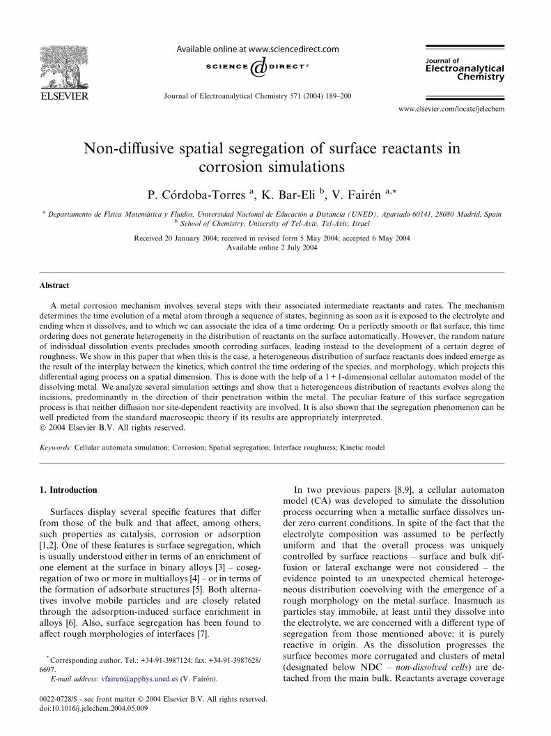
regation in contrast to the case shown in Fig. 4 that

shows the MðIÞads – segregation case, with this species

shifting preferential occupation to higher elevations.

Figs. 3 and 4 are particular examples of Cads orMðIÞads segregation, respectively. Different degrees of

segregation – including the possibility of no segregation,

i.e., homogeneous surface – are possible, depending on

the set of parameters values fRig. Metal cells (M cells)

constitute a distinct case for they always tend to accu-

mulate, on average, at low heights. It happens that at

low elevations an individual dissolution event uncovers,

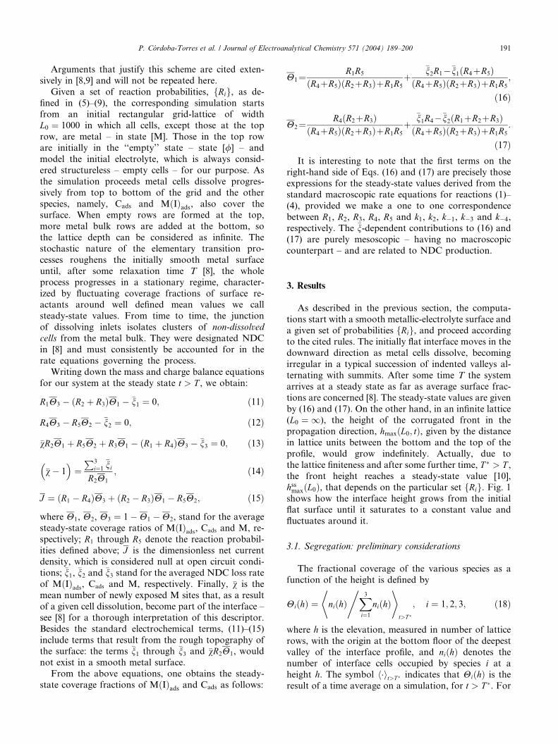
on average, more fresh new M sites than it does at highelevations, as shown in Fig. 5. �v, the average number of

newly exposed metal cells from the bulk after a disso-

lution event [8], decreases from bottom to top – the

decrease of �v with height is typical for the system and

occurs with all sets of parameters. This mechanism of

enlargement of the interface length is balanced by anNDC-stripping at interface protrusions, thus helping in

0 10 20 30 400,000

0,005

0,010

0,015

0,020

0,025

0,030

0,035

0,040

0,045

Ni(h )

h /lattice rows

N1

N2

N3

Fig. 4. Normalized number of MðIÞads cells (solid circles), Cads cells

(open circles) and M cells (triangles) vs. front height, h. This simulation

was carried with the following set of reaction probabilities:

R1 ¼ 8:94� 10�3, R2 ¼ 8:94� 10�4, R3 ¼ 0:0, R4 ¼ 8:13� 10�3,

R5 ¼ 1:48� 10�2.

0

h /lattice rows20 40 60

0

1

2

3

4

(h)χ

Fig. 5. Height dependence of �v – the average number of newly exposed

metal cells from the bulk after a dissolution event – calculated at the

steady state of simulation displayed in Figs. 1–3.

0 10 20 30 40 50 60 700

500

1000

1500

2000

tCA

(h)

h /lattice rows

Fig. 6. Averaged cellular automaton residence time, tCA, vs. front

height, h, corresponding to simulation of Figs. 1–3.


keeping the overall profile length fluctuating around aconstant value. Species segregation at these salient in-

terface parts explains why surface coverage for NDC

differs from the interface average, as is discussed further

at the end of Section 3.3.

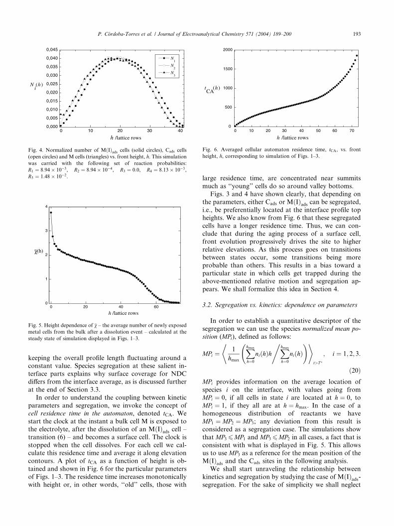
In order to understand the coupling between kinetic

parameters and segregation, we invoke the concept of

cell residence time in the automaton, denoted tCA. We

start the clock at the instant a bulk cell M is exposed tothe electrolyte, after the dissolution of an MðIÞads cell –transition (6) – and becomes a surface cell. The clock is

stopped when the cell dissolves. For each cell we cal-

culate this residence time and average it along elevation

contours. A plot of tCA as a function of height is ob-

tained and shown in Fig. 6 for the particular parameters

of Figs. 1–3. The residence time increases monotonically

with height or, in other words, ‘‘old’’ cells, those with

large residence time, are concentrated near summits

much as ‘‘young’’ cells do so around valley bottoms.

Figs. 3 and 4 have shown clearly, that depending on

the parameters, either Cads or MðIÞads can be segregated,

i.e., be preferentially located at the interface profile top

heights. We also know from Fig. 6 that these segregated

cells have a longer residence time. Thus, we can con-

clude that during the aging process of a surface cell,front evolution progressively drives the site to higher

relative elevations. As this process goes on transitions

between states occur, some transitions being more

probable than others. This results in a bias toward a

particular state in which cells get trapped during the

above-mentioned relative motion and segregation ap-

pears. We shall formalize this idea in Section 4.

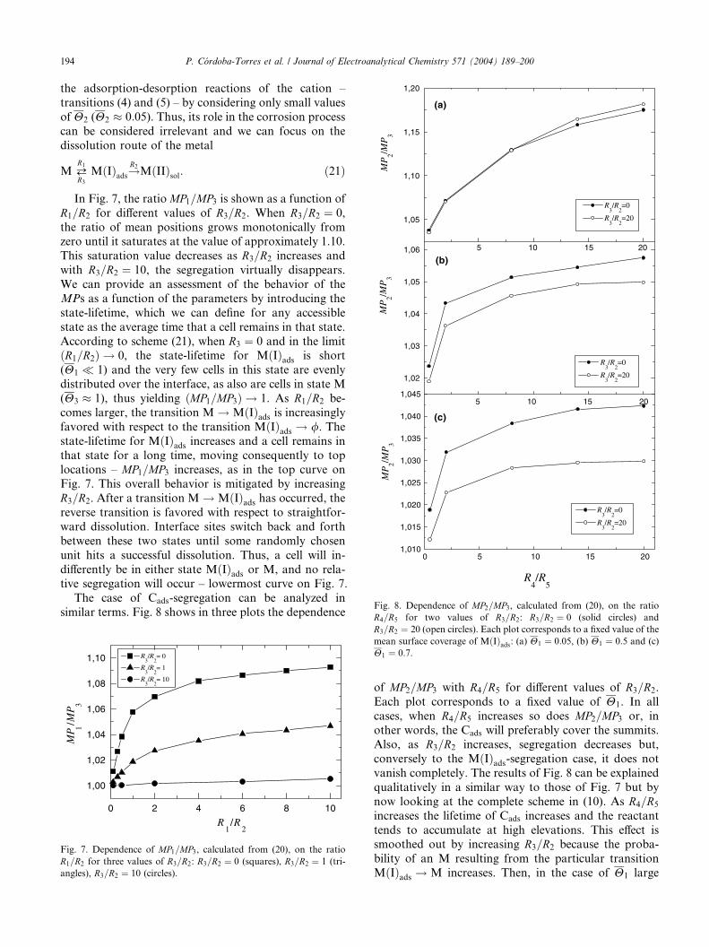
3.2. Segregation vs. kinetics: dependence on parameters

In order to establish a quantitative descriptor of the

segregation we can use the species normalized mean po-

sition (MPi), defined as follows:

MPi ¼1

hmax

Xhmax

h¼0

niðhÞhXhmax

h¼0

niðhÞ, ! +*

t>T �

; i ¼ 1; 2; 3:

ð20ÞMPi provides information on the average location of

species i on the interface, with values going from

MPi ¼ 0, if all cells in state i are located at h ¼ 0, to

MPi ¼ 1, if they all are at h ¼ hmax. In the case of a

homogeneous distribution of reactants we have

MP1 ¼ MP2 ¼ MP3; any deviation from this result isconsidered as a segregation case. The simulations show

that MP3 6MP1 and MP3 6MP2 in all cases, a fact that is

consistent with what is displayed in Fig. 5. This allows

us to use MP3 as a reference for the mean position of the

MðIÞads and the Cads sites in the following analysis.

We shall start unraveling the relationship between

kinetics and segregation by studying the case of MðIÞads-segregation. For the sake of simplicity we shall neglect

5 10 15 20

1,05

1,10

1,15

1,20

(a)

MP

2/ MP

3

5 10 15 20

1,02

1,03

1,04

1,05

1,06

R3/R

2=0

R3/R

2=20

MP

2/ MP

3

(b)

R3/R

2=0

R3/R

2=20

0 5 10 15 201,010

1,015

1,020

1,025

1,030

1,035

1,040

1,045

R3/R

2=0

R3/R

2=20

MP

2/ MP

3

(c)

R4/R

5

Fig. 8. Dependence of MP2=MP3, calculated from (20), on the ratio

R4=R5 for two values of R3=R2: R3=R2 ¼ 0 (solid circles) and


the adsorption-desorption reactions of the cation –

transitions (4) and (5) – by considering only small values

of H2 (H2 � 0:05). Thus, its role in the corrosion process

can be considered irrelevant and we can focus on the

dissolution route of the metal

M ¢R1

R3

MðIÞads!R2MðIIÞsol: ð21Þ

In Fig. 7, the ratio MP1=MP3 is shown as a function of

R1=R2 for different values of R3=R2. When R3=R2 ¼ 0,

the ratio of mean positions grows monotonically fromzero until it saturates at the value of approximately 1.10.

This saturation value decreases as R3=R2 increases and

with R3=R2 ¼ 10, the segregation virtually disappears.

We can provide an assessment of the behavior of the

MPs as a function of the parameters by introducing the

state-lifetime, which we can define for any accessible

state as the average time that a cell remains in that state.

According to scheme (21), when R3 ¼ 0 and in the limitðR1=R2Þ ! 0, the state-lifetime for MðIÞads is short

(H1 � 1) and the very few cells in this state are evenly

distributed over the interface, as also are cells in state M

(H3 � 1), thus yielding ðMP1=MP3Þ ! 1. As R1=R2 be-

comes larger, the transition M ! MðIÞads is increasinglyfavored with respect to the transition MðIÞads ! /. Thestate-lifetime for MðIÞads increases and a cell remains in

that state for a long time, moving consequently to toplocations – MP1=MP3 increases, as in the top curve on

Fig. 7. This overall behavior is mitigated by increasing

R3=R2. After a transition M ! MðIÞads has occurred, thereverse transition is favored with respect to straightfor-

ward dissolution. Interface sites switch back and forth

between these two states until some randomly chosen

unit hits a successful dissolution. Thus, a cell will in-

differently be in either state MðIÞads or M, and no rela-tive segregation will occur – lowermost curve on Fig. 7.

The case of Cads-segregation can be analyzed in

similar terms. Fig. 8 shows in three plots the dependence

0 2 4 6 8 10

1,00

1,02

1,04

1,06

1,08

1,10

MP 1

/ MP 3

R1/R

2

R3/R

2= 0

R3/R

2= 1

R3/R

2= 10

Fig. 7. Dependence of MP1=MP3, calculated from (20), on the ratio

R1=R2 for three values of R3=R2: R3=R2 ¼ 0 (squares), R3=R2 ¼ 1 (tri-

angles), R3=R2 ¼ 10 (circles).

R3=R2 ¼ 20 (open circles). Each plot corresponds to a fixed value of the

mean surface coverage of MðIÞads: (a) H1 ¼ 0:05, (b) H1 ¼ 0:5 and (c)

H1 ¼ 0:7.

of MP2=MP3 with R4=R5 for different values of R3=R2.

Each plot corresponds to a fixed value of H1. In all

cases, when R4=R5 increases so does MP2=MP3 or, inother words, the Cads will preferably cover the summits.

Also, as R3=R2 increases, segregation decreases but,

conversely to the MðIÞads-segregation case, it does not

vanish completely. The results of Fig. 8 can be explained

qualitatively in a similar way to those of Fig. 7 but by

now looking at the complete scheme in (10). As R4=R5

increases the lifetime of Cads increases and the reactant

tends to accumulate at high elevations. This effect issmoothed out by increasing R3=R2 because the proba-

bility of an M resulting from the particular transition

MðIÞads ! M increases. Then, in the case of H1 large

1,05

1,10

1,15

MP

/MP 1


(Fig. 8(c)) there are many MðIÞads cells distributed all

over the front height, meaning that more M cells will be

located at higher h. This is why MP2=MP3 decreases withrespect to the R3=R2 ¼ 0 case. The above effect resulting

from the MðIÞads ! M transition loses intensity whenH1 decreases (Fig. 8(a) and (b)) and so does the sepa-

ration between the curves.

0,95

1,00

2 4 6 8 10 12 14

L / L0

MP

/MP 2

MP

/MP 3

0,96

0,98

1,00

1,02

1,04

1,06

1,08

2 4 6 8 10 12 14

1,00

1,05

1,10

1,15

2 4 6 8 10 12 14

Fig. 9. The ratio MP=MPi vs. the roughness factor L=L0 for all the

simulations displayed in Figs. 7 and 8. Random dissolution (RD)

roughness factor value, ðL=L0ÞRD � 3:7, is represented by the vertical

dashed line.

3.3. Morphology vs. segregation

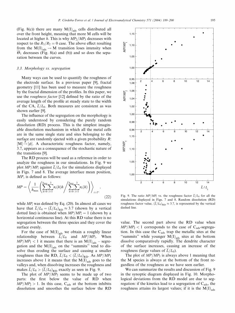
Many ways can be used to quantify the roughness of

the electrode surface. In a previous paper [9], fractal

geometry [11] has been used to measure the roughnessby the fractal dimension of the profiles. In this paper, we

use the roughness factor [12] defined by the ratio of the

average length of the profile at steady state to the width

of the CA, L=L0. Both measures are consistent as was

shown earlier [9].

The influence of the segregation on the morphology is

easily understood by considering the purely random

dissolution (RD) process. This is the simplest imagin-able dissolution mechanism in which all the metal cells

are in the same single state and sites belonging to the

surface are randomly ejected with a given probability R:

½M�!R ½/�. A characteristic roughness factor, namely,

3.7, appears as a consequence of the stochastic nature of

the transitions [9].

The RD process will be used as a reference in order to

analyze the roughness in our simulations. In Fig. 9 weplot MP=MPi against L=L0 for the simulations displayed

in Figs. 7 and 8. The average interface mean position,

MP, is defined as follows:

MP ¼ 1

hmax

Xhmax

h¼0

X3i¼1

niðhÞhXhmax

h¼0

X3i¼1

niðhÞ, ! +*

t>T �

;

ð22Þwhile MPi was defined by Eq. (20). In almost all cases we

have that L=L0 ¼ ðL=L0ÞRD � 3:7 (shown by a vertical

dotted line) is obtained when MP=MPi ¼ 1 (shown by a

horizontal continuous line). At this RD value there is no

segregation between the three species and they cover the

surface evenly.

For the case of MðIÞads we obtain a roughly linear

relationship between L=L0 and MP=MP1. WhenMP=MP1 < 1 it means that there is an MðIÞads – segre-

gation and the MðIÞads on the ‘‘summits’’ tend to dis-

solve thus eroding the surface and causing a smaller

roughness than the RD, L=L0 < ðL=L0ÞRD. As MP=MP1increases above 1 it means that the MðIÞads goes to the

valleys and, when dissolving increases the roughness and

makes L=L0 > ðL=L0ÞRD exactly as seen in Fig. 9.

The plot of MP=MP2 seems to be made up of twoparts: the first below the value of RD when

MP=MP2 > 1. In this case, Cads at the bottom inhibits

dissolution and smoothes the surface below the RD

value. The second part above the RD value when

MP=MP2 < 1 corresponds to the case of Cads-segrega-

tion. In this case the Cads trap the metallic sites at the

‘‘summits’’ while younger MðIÞads sites at the bottomdissolve comparatively rapidly. The dendrite character

of the surface increases, causing an increase of the

roughness (large values of L=L0).The plot of MP=MP3 is always above 1 meaning that

the M species is always at the bottom of the front re-

gardless of the roughness as we have seen earlier.

We can summarize the results and discussion of Fig. 9

in the synoptic diagram displayed in Fig. 10. Morpho-logical deviations from the RD model are due to seg-

regation: if the kinetics lead to a segregation of Cads, the

roughness attains its largest values; if it is the MðIÞads

M(I)ads

segregation

Cads

segregation

RD ModelRou

ghne

ss

Fig. 10. Scheme describing the relationship between the morphology of

the interface and the type of species segregation.

0,96 0,98 1,00 1,02 1,04 1,06 1,08 1,10 1,12 1,14 1,160,2

0,4

0,6

0,8

1,0

1,2

1,4

1,6

MP/MP2

Θ1N

DC /

Θ1

MP/MP1

0,96 0,98 1,00 1,02 1,04 1,06 1,08

0,0

0,2

0,4

0,6

0,8

1,0

1,2

1,4

1,6

Θ3N

DC /

Θ3

Θ2N

DC /

Θ2

0,98 1,00 1,02 1,04 1,06 1,08 1,10 1,12 1,14 1,16

0,0

0,2

0,4

0,6

0,8

1,0

MP/MP3

Fig. 11. Plots of the surface coverage of the species in the NDC, HNDC

i ,

relative to that on the interface, Hi, as a function of the species relative

mean position, MP=MPi, for all the simulations displayed in Figs. 7

and 8.


that is segregated, the profiles display a lower degree ofirregularity.

Segregation, however, does not always lead to a de-

parture from the RD model. There is a singular case of

segregation showing the same morphology as in the RD

model: the limit H1 ! 1. It is obtained when

R1=R2 ! 1 and R3=R2 ¼ 0. The interface is practically

covered by MðIÞads and MP=MP1 ! 1, but there is in-

stead a great segregation between MðIÞads and both Mand Cads (Fig. 7). We have thus MP=MP2 > 1 and

MP=MP3 > 1. The case to which we refer would corre-

spond to the limit point in the prolongation of the left

branch of the plots MP=MP2 and MP=MP3 in Fig. 9: as

R1=R2 ! 1 while R3=R2 ¼ 0, MP=MP2 and MP=MP3increase and L=L0 ! ðL=L0ÞRD.

We shall conclude the section by focusing on NDC

surface composition. As described in the introduction,the corrugated surface, formed by the dissolution pro-

cess, may break from time to time and detached clusters

of metal, designated non-dissolved cells – NDC, are

formed. It is reasonable to expect that the NDC will be

formed preferentially from the summits of the corru-

gated surface. Indeed, the plots of Fig. 11 are in agree-

ment with this expectation. The figure shows HNDC

i =Hi

as a function of MP=MPi, i.e., the average species cov-erage on the NDC, as compared to that of the interface

coverage, as a function of the species relative mean

position. The effect of the MðIÞads segregation is dis-

played in the first plot of Fig. 11: when the MðIÞadsspecies is located preferentially at the summits

(MP=MP1 < 1), the contours of NDC have more MðIÞadsthan expected, H

NDC

1 =H1 > 1. The Cads segregation case

behaves in a similar way: when MP=MP2 < 1 we observe

that HNDC

2 =H2 > 1, i.e., the NDC are covered prefer-

entially with Cads; again, our anticipation that the NDC

originate at the top is confirmed. Finally, in the last plot

of Fig. 9 we saw that MP=MP3 > 1 in all cases, showing

that the metal atoms are always located at the bottom.Therefore, one expects the NDC surface to be depleted

of the metal atoms; Fig. 11 shows that in all cases

0,25

0,30


HNDC3 =H3 < 1, i.e., there are less M cells on the surface

of NDC than on the bulk surface.

0,00

0,05

0,10

0,15

0,20

0,0

0,2

0,4

0,6

0,8

0 100 200 300 400 500 600 700

0,0

0,2

0,4

0,6

0,8

~

~

~

Θ3(t)

Θ2(t)

Θ1(t)

t

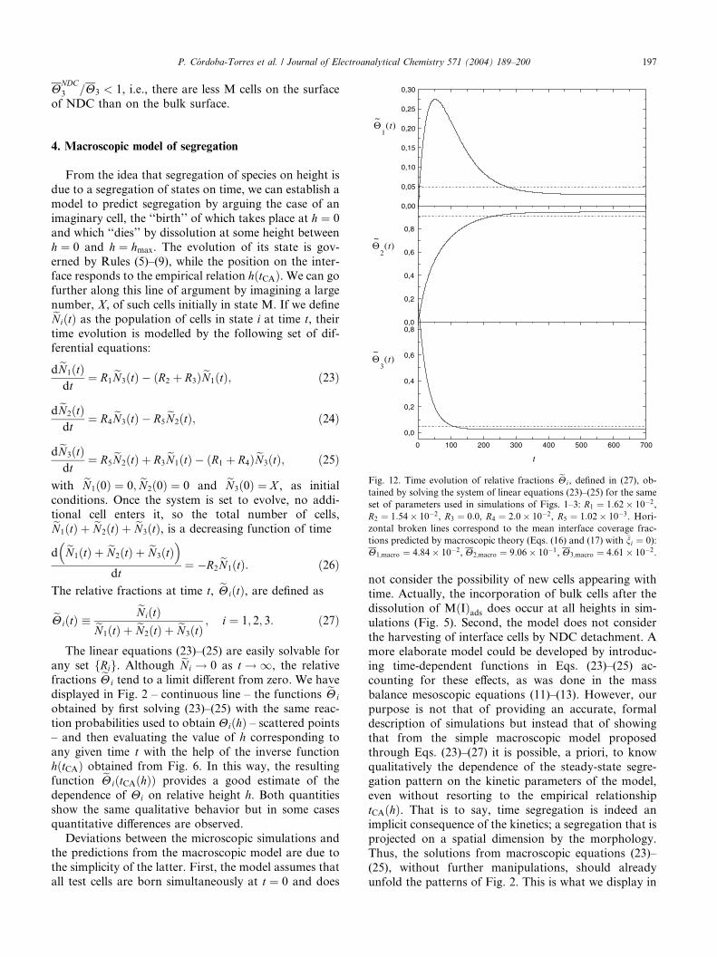
Fig. 12. Time evolution of relative fractions eHi, defined in (27), ob-

tained by solving the system of linear equations (23)–(25) for the same

set of parameters used in simulations of Figs. 1–3: R1 ¼ 1:62� 10�2,

R2 ¼ 1:54� 10�2, R3 ¼ 0:0, R4 ¼ 2:0� 10�2, R5 ¼ 1:02� 10�3. Hori-

zontal broken lines correspond to the mean interface coverage frac-

tions predicted by macroscopic theory (Eqs. (16) and (17) with �ni ¼ 0):

H1;macro ¼ 4:84� 10�2, H2;macro ¼ 9:06� 10�1, H3;macro ¼ 4:61� 10�2.

4. Macroscopic model of segregation

From the idea that segregation of species on height is

due to a segregation of states on time, we can establish a

model to predict segregation by arguing the case of an

imaginary cell, the ‘‘birth’’ of which takes place at h ¼ 0

and which ‘‘dies’’ by dissolution at some height between

h ¼ 0 and h ¼ hmax. The evolution of its state is gov-

erned by Rules (5)–(9), while the position on the inter-face responds to the empirical relation hðtCAÞ. We can go

further along this line of argument by imagining a large

number, X, of such cells initially in state M. If we defineeNiðtÞ as the population of cells in state i at time t, their

time evolution is modelled by the following set of dif-

ferential equations:

deN1ðtÞdt

¼ R1eN3ðtÞ � R2ð þ R3ÞeN1ðtÞ; ð23Þ

deN2ðtÞdt

¼ R4eN3ðtÞ � R5

eN2ðtÞ; ð24Þ

deN3ðtÞdt

¼ R5eN2ðtÞ þ R3

eN1ðtÞ � R1ð þ R4ÞeN3ðtÞ; ð25Þ

with eN1ð0Þ ¼ 0; eN2ð0Þ ¼ 0 and eN3ð0Þ ¼ X , as initial

conditions. Once the system is set to evolve, no addi-tional cell enters it, so the total number of cells,eN1ðtÞ þ eN2ðtÞ þ eN3ðtÞ, is a decreasing function of time

d eN1ðtÞ þ eN2ðtÞ þ eN3ðtÞ� �

dt¼ �R2

eN1ðtÞ: ð26Þ

The relative fractions at time t, eHiðtÞ, are defined as

eHiðtÞ �eNiðtÞeN1ðtÞ þ eN2ðtÞ þ eN3ðtÞ

; i ¼ 1; 2; 3: ð27Þ

The linear equations (23)–(25) are easily solvable for

any set fRig. Although eNi ! 0 as t ! 1, the relative

fractions eHi tend to a limit different from zero. We have

displayed in Fig. 2 – continuous line – the functions eHi

obtained by first solving (23)–(25) with the same reac-

tion probabilities used to obtain HiðhÞ – scattered points– and then evaluating the value of h corresponding to

any given time t with the help of the inverse function

hðtCAÞ obtained from Fig. 6. In this way, the resulting

function eHiðtCAðhÞÞ provides a good estimate of the

dependence of Hi on relative height h. Both quantities

show the same qualitative behavior but in some cases

quantitative differences are observed.

Deviations between the microscopic simulations andthe predictions from the macroscopic model are due to

the simplicity of the latter. First, the model assumes that

all test cells are born simultaneously at t ¼ 0 and does

not consider the possibility of new cells appearing with

time. Actually, the incorporation of bulk cells after the

dissolution of MðIÞads does occur at all heights in sim-

ulations (Fig. 5). Second, the model does not consider

the harvesting of interface cells by NDC detachment. A

more elaborate model could be developed by introduc-ing time-dependent functions in Eqs. (23)–(25) ac-

counting for these effects, as was done in the mass

balance mesoscopic equations (11)–(13). However, our

purpose is not that of providing an accurate, formal

description of simulations but instead that of showing

that from the simple macroscopic model proposed

through Eqs. (23)–(27) it is possible, a priori, to know

qualitatively the dependence of the steady-state segre-gation pattern on the kinetic parameters of the model,

even without resorting to the empirical relationship

tCAðhÞ. That is to say, time segregation is indeed an

implicit consequence of the kinetics; a segregation that is

projected on a spatial dimension by the morphology.

Thus, the solutions from macroscopic equations (23)–

(25), without further manipulations, should already

unfold the patterns of Fig. 2. This is what we display in

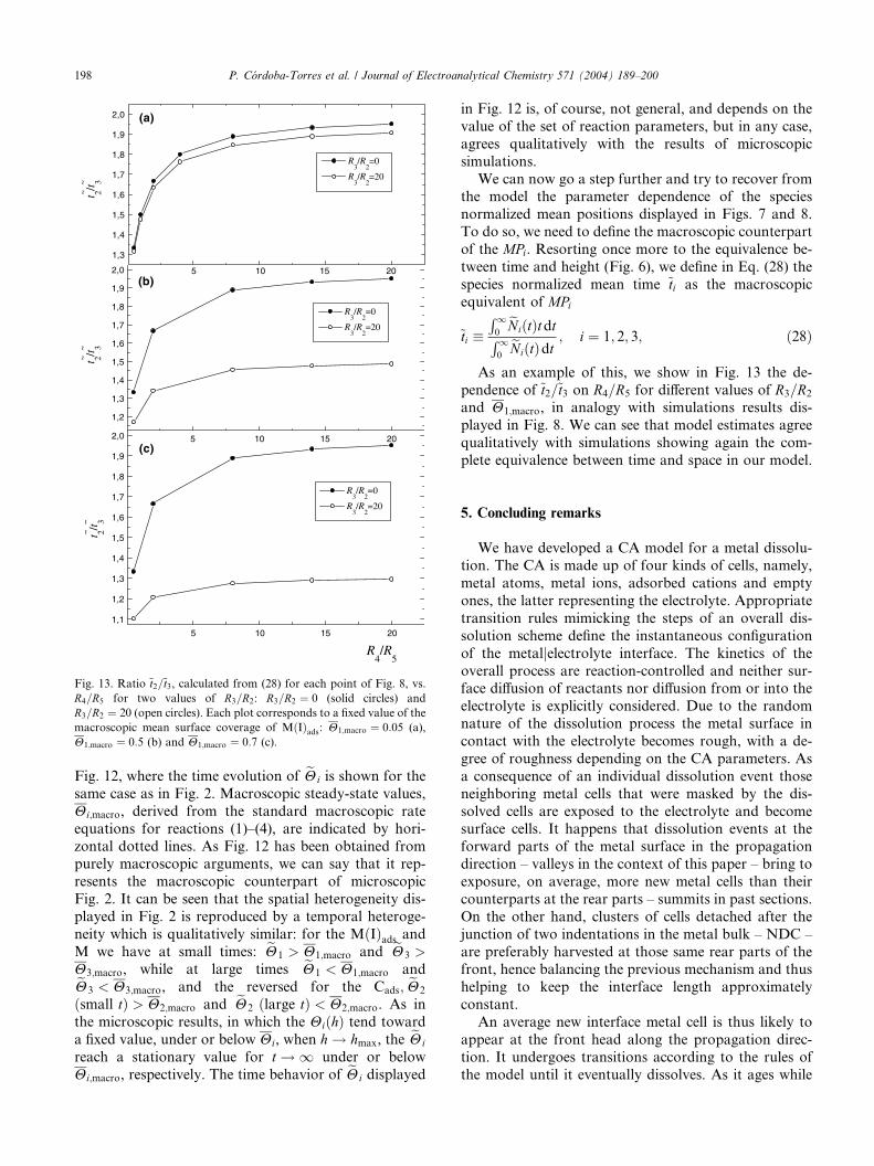
5 10 15 20

5 10 15 20

5 10 15 20

1,3

1,4

1,5

1,6

1,7

1,8

1,9

2,0

~~

t 2/ t 3

~~

t 2/ t 3

(a)

R3/R

2=0

R3/R

2=20

1,2

1,3

1,4

1,5

1,6

1,7

1,8

1,9

2,0

R3/R

2=0

R3/R

2=20

(b)

1,1

1,2

1,3

1,4

1,5

1,6

1,7

1,8

1,9

2,0

R3/R

2=0

R3/R

2=20

~~

t 2/ t 3

(c)

R4/R

5

Fig. 13. Ratio ~t2=~t3, calculated from (28) for each point of Fig. 8, vs.

R4=R5 for two values of R3=R2: R3=R2 ¼ 0 (solid circles) and

R3=R2 ¼ 20 (open circles). Each plot corresponds to a fixed value of the

macroscopic mean surface coverage of MðIÞads: H1;macro ¼ 0:05 (a),

H1;macro ¼ 0:5 (b) and H1;macro ¼ 0:7 (c).


Fig. 12, where the time evolution of eHi is shown for the

same case as in Fig. 2. Macroscopic steady-state values,

Hi;macro, derived from the standard macroscopic rate

equations for reactions (1)–(4), are indicated by hori-

zontal dotted lines. As Fig. 12 has been obtained frompurely macroscopic arguments, we can say that it rep-

resents the macroscopic counterpart of microscopic

Fig. 2. It can be seen that the spatial heterogeneity dis-

played in Fig. 2 is reproduced by a temporal heteroge-

neity which is qualitatively similar: for the MðIÞads andM we have at small times: eH1 > H1;macro and eH3 >H3;macro, while at large times eH1 < H1;macro andeH3 < H3;macro, and the reversed for the Cads; eH2

ðsmall tÞ > H2;macro and eH2 ðlarge tÞ < H2;macro. As in

the microscopic results, in which the HiðhÞ tend toward

a fixed value, under or below Hi, when h ! hmax, the eHi

reach a stationary value for t ! 1 under or below

Hi;macro, respectively. The time behavior of eHi displayed

in Fig. 12 is, of course, not general, and depends on the

value of the set of reaction parameters, but in any case,

agrees qualitatively with the results of microscopic

simulations.

We can now go a step further and try to recover fromthe model the parameter dependence of the species

normalized mean positions displayed in Figs. 7 and 8.

To do so, we need to define the macroscopic counterpart

of the MPi. Resorting once more to the equivalence be-

tween time and height (Fig. 6), we define in Eq. (28) the

species normalized mean time ~ti as the macroscopic

equivalent of MPi

~ti �R10eNiðtÞtdtR1

0eNiðtÞdt

; i ¼ 1; 2; 3; ð28Þ

As an example of this, we show in Fig. 13 the de-

pendence of ~t2=~t3 on R4=R5 for different values of R3=R2

and H1;macro, in analogy with simulations results dis-

played in Fig. 8. We can see that model estimates agree

qualitatively with simulations showing again the com-

plete equivalence between time and space in our model.

5. Concluding remarks

We have developed a CA model for a metal dissolu-

tion. The CA is made up of four kinds of cells, namely,

metal atoms, metal ions, adsorbed cations and empty

ones, the latter representing the electrolyte. Appropriate

transition rules mimicking the steps of an overall dis-

solution scheme define the instantaneous configuration

of the metaljelectrolyte interface. The kinetics of the

overall process are reaction-controlled and neither sur-face diffusion of reactants nor diffusion from or into the

electrolyte is explicitly considered. Due to the random

nature of the dissolution process the metal surface in

contact with the electrolyte becomes rough, with a de-

gree of roughness depending on the CA parameters. As

a consequence of an individual dissolution event those

neighboring metal cells that were masked by the dis-

solved cells are exposed to the electrolyte and becomesurface cells. It happens that dissolution events at the

forward parts of the metal surface in the propagation

direction – valleys in the context of this paper – bring to

exposure, on average, more new metal cells than their

counterparts at the rear parts – summits in past sections.

On the other hand, clusters of cells detached after the

junction of two indentations in the metal bulk – NDC –

are preferably harvested at those same rear parts of thefront, hence balancing the previous mechanism and thus

helping to keep the interface length approximately

constant.

An average new interface metal cell is thus likely to

appear at the front head along the propagation direc-

tion. It undergoes transitions according to the rules of

the model until it eventually dissolves. As it ages while


the metaljelectrolyte interface keeps propagating, it is

subjected to a displacement, relative to the mean posi-

tion of the front in a direction opposite to that of

propagation. Therefore, the cell positions along the

propagation direction depend monotonically on theirage and thus a space–time relationship can be estab-

lished.

By controlling the CA parameters we can define

which transition or step is slowest. The reactants par-

ticipating in the slowest will have a longer lifetime than

the other intervening species and consequently surface

cells will be trapped in that particular state. As they age

they tend to concentrate at the back of the interfacealong the propagation direction, thus unfolding a het-

erogeneous interface along that same direction. We

speak of a segregation of that particular reactant.

Here, we have dealt with two intermediate reactants:

a metal ion that takes part in the metal dissolution route

and an adsorbed cation. From a morphological point of

view this brings opposite consequences. Metal ion –

MðIÞads – segregation has a leveling effect on the surface,diminishing roughness. On the contrary, by delaying

dissolution the adsorbed cation – Cads – segregation

promotes dendrite formation as large portions of the

interface covered by cells in state Cads remain lagging

behind while dissolution proceeds within deep cuts into

the metal bulk, thus enhancing roughness.

From a kinetic point of view, the importance of the

spatial heterogeneity becomes crucial when bimolecularreactions are included in the reactive scheme. That is the

case of the Tafel reaction: Cads þ Cads ! C2;sol. It has

been shown [13] that, even in a motionless scenario, the

Tafel reaction is well described by fractional order ki-

netics in which the reaction order depends on the aver-

age local coverage of Cads around a Cads, namely, Hlocal

2 .

When this local coverage is equal to the global average,

i.e., Hlocal

2 ¼ H2, the second-order kinetics predicted bythe mean field (MF) theory – which is essentially based

on a perfect mixing of reactants – is then recovered. If,

however, we have Hlocal

2 6¼ H2, then the reaction order

differs from the value of two and the kinetics departs

from the standard macroscopic equations derived from

the MF approach. When the distribution of Cads on the

surface is heterogeneous, as in the Cads-segregation case,

we have Hlocal

2 6¼ H2 and, consequently, the kinetics arecharacterized by a fractional reaction order. If the seg-

regation is very pronounced, we may have Hlocal

2 � 1,

thus giving first-order kinetics for the Tafel reaction.

Finally, a simple macroscopic model that imitates the

CA behavior by describing the evolution of a closed

population of cells was developed and its results com-

pared to those of the CA. As such, this macroscopic

model consists of a set of ordinary differential equationsfor the time evolution of the species coverage fractions.

Once the equations were integrated and the time vari-

able projected into a space variable a good qualitative

agreement was obtained with the CA. This is not sur-

prising inasmuch as the segregation is actually an effect

of the reaction kinetics – diffusion of reactants is not

allowed – and becomes apparent if the appropriate

projection on a spatial scale is conveniently chosen.Consequently, if time and space can be mapped indif-

ferently into each other and the reaction kinetics gov-

erns the ordering in time, then segregation should be

inferable from an integration of the standard macro-

scopic equations without resorting to any spatial map-

ping: that is, reading the time axis as if it was a spatial

coordinate. As shown, this is perfectly possible. The

standard macroscopic equations can give the clue tospatial heterogeneity obtained in the simulations.

Preliminary results obtained from simulations of

more complex reactive schemes, including several routes

of dissolution or considering up to six intermediate

species for the metal, have shown that the conclusions

obtained in the present work are independent of the

model used: states corresponding to reactants partici-

pating in slow reactive steps have longer state-lifetimes,leading to a segregation pattern of those species. This

has a feedback effect on the morphology: if the segre-

gated reactant takes part in the direct dissolution route

of the metal, i.e., it is a metal anion, the resulting mor-

phology has a lower degree of irregularity than the RD

model. If, on the contrary, this is not the case and the

segregated species belongs to an alternative route of

dissolution, it may lead to a high degree of roughness.The macroscopic model developed in Section 4, when it

is properly adapted for the specific reactive scheme used,

has also proved to be very useful in the prediction and

analysis of the segregation results. These results will be

covered in a forthcoming publication.

Acknowledgements

K. Bar-Eli has enjoyed a sabbatical year from The

Ministerio de Educaci�on y Ciencia, Spain. The authors

express their thanks to R.P. Nogueira for his fruitful

discussions.

References

[1] G.A. Somorjai, Introduction to Surface Chemistry and Catalysis,

Wiley, New York, 1994.

[2] C. Stampfl, M.V. Ganduglia-Pirovano, K. Reuter, M. Scheffler,

Surf. Sci. 500 (2002) 368.

[3] M. Polak, L. Rubinovich, Surf. Sci. Rep. 38 (2000) 127.

[4] L.N. Gumen, E.P. Feldman, V.M. Yurchenko, T.N. Mel’nik,

A.A. Krokhin, Surf. Sci. 445 (2000) 526.

[5] V.P. Zhdanov, Surf. Sci. 500 (2002) 966.

[6] E. Christoffersen, P. Stoltze, J.K. Nørskov, Surf. Sci. 505 (2002)

200.

[7] B. Koiller, R.B. Capaz, H. Chacham, Phys. Rev. B 60 (1999) 1787.


[8] P. C�ordoba-Torres, R.P. Nogueira, L. de Miranda, L. Brenig, J.

Wallenborn, V. Fair�en, Electrochim. Acta 46 (2001) 2975.

[9] P. C�ordoba-Torres, R.P. Nogueira, V. Fair�en, J. Electroanal.

Chem. 529 (2002) 109.

[10] A.L. Barab�asi, H.E. Stanley, Fractal Concepts in Surface Growth,

Cambridge University Press, Cambridge, 1995.

[11] B.B. Mandelbrot, The Fractal Geometry of Nature, Freeman, San

Francisco, CA, 1997.

[12] A.J. Arvia, R.C. Salvarezza, J.M. Vara, Electrochim. Acta 37

(1992) 2155.

[13] P. C�ordoba-Torres, R.P. Nogueira, V. Fair�en, J. Electroanal.

Chem. 560 (2003) 25.

Non-diffusive spatial segregation of surface reactants in corrosion simulations

Documents

Transcript of Non-diffusive spatial segregation of surface reactants in corrosion simulations