Homeownership, Community Interactions, and Segregation

Karla Hoff Arijit Sen The World Bank Jawaharlal Nehru University

khoff@worldbank.org senarijit@vsnl.net

This revision: March 2004

Abstract

We consider a multi-community city where community quality is linked to residents’ civic efforts like

being proactive in preventing crime and in ensuring the quality of publicly provided goods. Home-

ownership increases incentives for such efforts, but credit market imperfections force the poor to rent.

Within-community externalities can lead to segregated cities − with the rich living with rich in healthy

homeowner communities, and the poor living with poor in dysfunctional renter communities. The

pattern of tenure segregation across communities in the US accords well with our prediction. We study

alternative tax-subsidy policies to alleviate inefficiencies in the housing market, and identify the winners

and losers under such policies.

Support from the MacArthur Network on Inequality and Economic Performance is gratefully acknowledged. Jyotsna Puri and Varsha Venkatesh provided valuable research assistance. We thank an anonymous referee, Roland Bénabou, Tim Besley, Avinash Dixit, Debraj Ray, and Tony Yezer for helpful comments. We have also benefited from comments by seminar participants at Boston, Brookings, Cornell, Fannie Mae, George Washington, MIT, Paris, Princeton, Toulouse, Wisconsin, and the World Bank. The views expressed in this paper are the authors’ and should not be attributed to their employers.

Pub

lic D

iscl

osur

e A

utho

rized

Pub

lic D

iscl

osur

e A

utho

rized

Pub

lic D

iscl

osur

e A

utho

rized

Pub

lic D

iscl

osur

e A

utho

rized

“New Yorkers who lived through the arson and looting that ravaged the city during the blackout of 1977 were understandably edgy when the lights went out on August 14 [2003]. But it was clear by late evening that … [t]his night did not belong to arsonists or looters. … An important difference between this blackout and the last one is the massive, publicly financed reconstruction effort that has rebuilt neighborhoods like the South Bronx from scratch. The program, begun by Mayor Edward Koch in the 80's, has produced more than 200,000 affordable apartments and houses, revitalizing burned-out communities and turning record numbers of New Yorkers into homeowners with a vested interest in keeping their areas safe.”

New York Times editorial, 8/24/2003

The nature of communities has become a central concern in every society. A large empirical literature

shows that homeownership makes a difference for civic quality (see the references below). In the US,

many cities are segregated between homeowner communities and renter communities (see the evidence

in Section 1.2); there is a high correlation between the latter and violent crime-ridden neighborhoods

(see Sampson et al. 1997); and growing up in such neighborhoods has a profound negative impact on

health, personal development, and school outcomes (see Leventhal and Brooks-Gunn 2000).

The existing theoretical literature on homeownership does not adequately explain these phenomena.

Some authors do not model the dependence of housing tenure choice on community characteristics,

treating the latter as fixed (e.g., Henderson and Ioannides 1983). Others suggest that crime in renter

communities is a simple consequence of poverty: “it is the poverty associated with poor housing, rather

than the housing per se, that causes these costly social problems” (Rosen 1985, p.378).

This paper presents a model that challenges these views. We show that households with identical

preferences and similar abilities to create healthy neighborhoods may nonetheless self-organize into

communities with starkly different characteristics. An interplay of within-community externalities and

market forces can lead to cities that are segregated by tenure and income − with the rich living with rich

in homeowner communities with well-functioning civic environments, and the poor living with poor in

dysfunctional renter communities. The predicted segregation between homeowners and renters accords

well with the actual housing tenure segregation in the US, which we document for the first time.

Our model provides a theoretical framework to evaluate alternative housing policies. The

centerpiece of US urban development policy is to expand homeownership among low-income

households (Department of Housing and Urban Development, 1991). It has been claimed that “a critical

mass of homeowners can turn around the dynamic of a distressed neighborhood” (Washington Post,

1

4/12/97), and that “if there is a silver bullet in urban redevelopment, it is homeownership” (New York

Times, 4/16/98). Recent policy initiatives have also focused on the social benefits of promoting co-

residence of homeowners and renters in a community. The Moving to Opportunity demonstration,

which has been operating in five US cities since 1994, involves moving families from the least desirable

housing projects to safer home-owning neighborhoods (see Katz et al., 2001). We use our model to

analyze both kinds of policies − housing subsidy schemes to raise homeownership rates, and policies to

encourage homeowners and renters to live together.

Our premise is that a community’s civic environment − its local institutions, the crime situation, etc.

− greatly influences the well-being of residents. Residents can expend effort to enhance the civic quality

of their homes and their community − improve security by being vigilant against crime; ensure quality

supply of publicly provided goods by participating in the running of local institutions, voting in local

elections, and demonstrating against government inaction, etc.. Such civic efforts share the following

features: individual effort generates positive spillovers for community neighbors, there are complemen-

tarities in the costs and benefits to such effort, and sustained civic efforts lead to durable improvements

in the community environment and increases in property values (see Section 1.1 for evidence).1

However, individual effort is not contractible. A household chooses its effort level in its self-

interest, given its perceived private returns from such effort. That is why ownership matters. While all

residents gain to the same extent from an improvement in civic quality, homeowners also gain from the

increase in their property value. As a result, homeowners are more likely to expend greater civic effort.

But then why don’t all community residents become homeowners? Because, given imperfections in the

credit market, the cost of borrowing to purchase a home is substantially higher for the poorer residents.2

In a city with many communities, we study the implications of these features on the effort, tenure,

and location decisions of households with different incomes, and on the community outcomes that these

1 Another important feature of most civic actions is that one has to be a community resident to take effective actions. ‘Absentee landlords’ will have much higher costs than residents of obtaining information about shocks to the home and the community, and of responding to such shocks. Further, they will not have the same incentives to take such actions since they are not directly affected by community quality but only by its effect on property values. 2 Down-payment and debt service provisions prevent a majority of renters in the US from becoming homeowners. Savage (1999) reports that in 1995, 70% of families that rented in the US were unable to purchase a $20,000 home.

2

decisions generate. Formally, we construct a ‘multi-community social interactions model’ that links

community characteristics with individual actions.3 We embed in it an agency problem that arises from

the non-contractibility of effort. The co-existence of local interaction effects and a moral hazard

problem has the following consequences for community formation and individual welfare.

First, there is a ‘wealth effect on incentives’: within a community, homeowners are richer than

renters and, since ownership contracts provide better incentives, expend greater civic effort.4 Second,

individual tenure decisions depend on the community tenure distribution since that influences the returns

to investing in a home. As a result, there exists a within-community ‘social multiplier’: when some

households switch from renting to owning, that by itself induces their neighbors to make similar

switches. This can lead to a coordination problem and generate multiple equilibria.

Third, if homeowners are willing to pay even slightly more than renters for an improvement in

community quality (which will be the case under plausible conditions), they will ‘agglomerate’ by out-

bidding renters. This will lead to tenure segregation, with homeowner communities having a better civic

environment and higher property values than renter communities. Finally, it may be the case that if one

household is richer than another, the former is willing to pay more for an improvement in community

quality than the latter. Then there will be segregation both by tenure and by income, and all residents of

a ‘better’ community will be richer than all residents of a ‘worse’ one.5

We thus provide an explanation of the co-existence ‘good’ and ‘bad’ communities that does not rely

upon differences among individuals in preferences or abilities, but upon differences among collectivities

that arise endogenously due to positive feedback effects of non-contractible effort.

3 Schelling (1971), de Bartolome (1990), Bénabou (1993, 1996), and Durlauf (1996) are seminal papers in the social interactions literature; also see the surveys by Fernandez (2001) and Durlauf (2003). 4 In this, our paper relates to agency models exhibiting wealth effects on incentives by Galor and Zeira (1993), Legros and Newman (1996), and Mookherjee and Ray (2002) among others. 5 In our ‘behavioral peer groups’ model, an agent’s utility is affected by the behavior of his neighbors (i.e., their effort choice) and not by their types (i.e., rich or poor). As a result, the forces that lead to segregation with respect to endogenous behavior (tenure segregation) are not identical to those that lead to segregation with respect to exogenous types (income segregation). In Section 4.2, we show the connections between these two dimensions of segregation.

Bénabou (1993) and Brock and Durlauf (2001) also model behavioral peer groups. In the former paper, agents behave differently in equilibrium because the technology exhibits diminishing returns to behaving in the same way as others. In the latter paper, exogenous preference differences cause behavior heterogeneity. Helsley and Strange (2000) consider a model where heterogeneous residents choose different actions with local externalities; the authors study the secession of a group of residents from a single community, and not free-mobility equilibria in a multi-community city.

3

An important consequence of this is that community equilibria need not be constrained Pareto

efficient. Specifically, there may be ‘too few’ homeowners in a city because of uncompensated

externalities from homeownership. This problem can be compounded by a coordination failure in tenure

choice. In addition, equilibrium tenure segregation may be inefficient: the agglomeration of

homeowners and renters in distinct communities can adversely affect average community quality.

We study alternative tax-subsidy policies that address each kind of inefficiency.6 We show that

housing subsidy policies can enhance efficiency by improving the city’s ‘tenure profile,’ and can do so

more cost-effectively when subsidies can be appropriately ‘targeted.’ We then present a novel tax-

subsidy scheme that can induce a ‘stable integration’ of homeowners and renters.

An important feature of such policies is that they are likely to generate both ‘winners’ and ‘losers.’

While middle class homeowners benefit from a housing subsidy scheme (especially those who become

homeowners under the scheme), low-income renters can be hurt as the scheme is likely to raise their

rents. The identities of winners and losers will be very different under a policy that integrates

communities by tenure − co-residence with homeowners can make all renters better off while all home-

owners can be worse off as property values fall. This helps understand the opposition that desegregation

schemes have generally met. For instance, in a protracted legal conflict over the right of a non-profit

organization to build low-income housing in a New Jersey community, the community would accept

low-income residents if they were homeowners, but not if they were renters (Newsday 3/7/96).

We proceed as follows. Section 1 presents the empirical evidence that motivates our study. We set

up the model in Section 2, and solve for individual tenure choices in Section 3. Community equilibria

are characterized in Section 4. In Section 5, we discuss the nature of inefficiencies in such equilibria and

study corrective policies. Section 6 contains our concluding remarks. Appendix I discusses a general

agency model of tenure contracting; proofs are presented in Appendix II; and Appendix III contains an

example of equilibria in a two-community city.

6 This complements and extends the policy analysis of Fernandez and Rogerson (1996), who study a model where households with different incomes have different preferences over locally-financed education. Their study is carried out in a simpler framework where there is no housing market, and thus there are no ‘price effects’ of relocating a household from one community to another.

4

1. Empirical Evidence

1.1 Community Interactions and Incentive Effect of Homeownership

In this section, we report the findings of existing empirical studies that document community interaction

effects, and those that demonstrate that homeowners are ‘better citizens’ than renters.

In a study of Chicago neighborhoods, Sampson et al. (1997) find that the most important influence

on a community’s crime rate is the residents’ willingness to respond to threats to community safety.

Besley and Burgess (2002) and Stromberg (2004) show that state and local governments are more

responsive in areas where information flows are more developed and political participation is greater.

These studies indicate that individual actions generate within-community spillovers. While a

household is primarily motivated by self-interest to take such actions, e.g., improve the safety of its

home, ensure adequate access to publicly provided goods, etc., its effort creates an ‘impure local public

good’ − a good that provides utility to the household and raises the market value of its home, and also

provides similar benefits to its community neighbors, albeit to a lesser degree.

Cohen and Dawson (1993) find that living in extremely poor communities, where the civic

participation of the poor is low due to their limited education and income, leads the non-poor to

politically disengage as well. This indicates the existence of complementarities between individual and

group actions. Specifically, when the aim is to improve the functioning of local institutions and/or to

deter crime, there is obvious ‘strength in numbers.’ An attempt to bring criminals to justice can be very

costly for an individual if he is working alone. In a study of the central district of a major Northeastern

US city, Merry (1981, p.142) estimates that 40% of burglaries of black families are retaliatory acts

against households that are perceived to have ‘big mouths’ (i.e., those who report crimes to the police).

A number of studies show that the benefits of civic actions persist over time and raise property

values. Pargal and Wheeler (1996) find that pressure from community residents is very effective in

long-term reduction in pollution from industrial plants, and Smith and Huang (1995) show that

reductions in air pollution are capitalized into housing prices. Buck et al. (1991) establish that decreases

in crime are strongly positively related to housing prices.

There is also substantial empirical evidence that controlling for observables, homeowners expend

5

greater civic effort than renters. Table 1 summarizes some recent studies that find that homeowners are

significantly more likely to be engaged in neighborhood activism when facing a threat to its home and

community (Cox 1982), to be involved in community organizations (Rohe and Stegman 1994), and to

vote in local elections (Verba et al. 1995, DiPasquale and Glaeser 1999).

The joint hypothesis of the incentive effect of homeownership and durable improvements in home

and community quality resulting from residents’ civic efforts predicts that property values should be

rising in the number of homeowners in a community. Controlling for the composition of a community

by race and education, Coulson et al. (2001, p.5) find that “higher rates of ownership in neighborhoods

are indeed accompanied by higher housing prices within the neighborhood.”

1.2 Tenure Segregation

We now present primary evidence that homeowners desire to co-reside with other homeowners. We

utilize the 1990 US Census data to empirically study the pattern of tenure segregation across

communities in the US. We use data on the ten largest metropolitan areas (MSAs), covering 37% of the

population. We proxy for ‘communities’ with census tracts, which are areas of between 2,500 and 8,000

people separated by boundaries such as rivers, highways, or major streets.7

We report the commonly used index of spatial segregation − the ‘dissimilarity index,’ analyzed in

Massey and Denton (1988). In our context, the index answers the question: Within an MSA, what

fraction of the population needs be relocated so that each tract has the same proportion of homeowners

and renters as that of the MSA? The index ranges from zero (when all tracts have the same ratio of

owners to renters) to one (when owners and renters do not co-reside in any tract). Since there is

evidence that race and income cause segregation (Schelling 1971, Cutler et al. 1999), we calculate the

index separately for families with different attributes. The index for households with attribute χ is:

Dissimilarity index = 2

∑ −i

ii

OHoh

RHrh

χ

χ

χ

χ

,

7 The data show that poorer families are more likely to rent; the fraction of families with children who are homeowners rises from 31% to 65% as annual income rises from the $15,000-25,000 to the $35,000-50,000 bracket.

6

where, for families with attribute χ, rhiχ (resp., ohiχ) is the number of renter (resp., owner) households in

the tract, and RHχ (resp., OHχ) is the total number of renter (resp., owner) households in the MSA.

Table 2 shows that the dissimilarity index is moderate to high for every income class and race. In

each income bracket, approximately 60% to 80% of black households would have to move for each tract

to have the same owner/renter composition as that of the MSA. The corresponding number for non-

black families with children ranges from 40% to 60%.8 This pattern of tenure segregation cannot be

explained by race or income or the presence of children, because it occurs within household groups with

similar attributes. Our analysis provides an explanation for this phenomenon.

2. The Model

Consider a city consisting of N (>1) communities, each having single-family homes of measure 1/N.

The housing units are physically identical, and are owned by a large number of infinitely-lived risk-

neutral real estate companies. A generation of households moves into the city at the beginning of every

period, and moves out at the end of the period (when the next generation moves in).9 For simplicity, we

take the number of households in every generation to be the same as the total number of homes in the

city: a continuum of measure one. In each generation, households are identical in all respects except

their current (endowed) income y, which is distributed across households according to F(.) on an interval

[y−, y+]. Each household’s (common) future income is w.

Our model is essentially static in that we focus on the behavior of a particular generation of

households. After a household has received its income y, it selects a home in one of the N communities

and negotiates a ‘tenure contract’ with the relevant real estate company. This contract is a pair {α, β}:

for an up-front payment β, the household acquires the right of residence for the period and the right to a

fraction α of the price of the home at the end of the period. The fraction α is a household’s home equity

8 The extent of tenure segregation is comparable to that of racial segregation. Cutler et al. (1999) find that for blacks and whites in all US cities in 1990, the dissimilarity index was 0.56. We find that the pattern of tenure segregation is similar across the ten MSAs, but Table 2 reports only a weighted average (with weights based on MSA population). 9 We think of a generation as composed of families who enter the city when the family is formed, reside there during the working lives of the adults, and move away when they retire. Our assumption that real estate companies own the homes simplifies the analysis without being crucial to it; see Bénabou (1996) for a similar assumption.

7

share. We will refer to a contract with a sufficiently large α (defined in (2)) as an ‘ownership

contract’.10 A contract with α = 0 is a ‘rental contract’; we let ρ denote the rent (i.e., β = ρ for α = 0).

2.1 Community Quality

A household’s utility from living in a home derives from the ‘civic quality’ of the home − its security,

the quality of publicly provided community goods, etc. − which, in turn, depends on the resident’s own

civic effort and on the efforts of his community neighbors. We assume that the initial civic quality is the

same for all homes in the city, and set its value at zero. We then study how differences in household

effort lead to heterogeneity in civic quality across communities.

After signing a tenure contract, each household decides on its level of civic effort. While there are

many dimensions to such effort, for brevity we assume that there are two actions, a ∈ {e, n}, where e is

high effort and n is negligible effort. The ‘current’ civic quality of a home is q(a, x), where x is the

fraction of community residents who expend high effort. We refer to x as the community effort level;

this is what distinguishes one community from another. While a home’s civic quality obviously rises in

resident effort, i.e., q(e, x) > q(n, x), we assume that it increases in community effort x − a ‘spillover

effect,’ and that a household’s marginal return to effort also increases in x − a ‘complementarity effect.’

ASSUMPTION 1 (Community Interaction Effects): (i) qx(a, x) > 0, and (ii) qx(e, x) > qx(n, x).11

The evolution of housing prices depends on the evolution of home quality. We take the ‘future’

civic quality of a home (i.e., its quality at the beginning of the following period) to be [γ.q(a, x)], where γ

∈ (0, 1) is the one-period depreciation factor; thus, a part of the current quality persists in the future. To

keep things simple, we take as primitive the ‘future price function’ P(γq), with P′(⋅) > 0. We let p(a, x) ≡

P(γ.q(a, x)), and assume that P(⋅) is not too concave so that a and x affect the future price of a home in

10 This is similar to the limited equity housing contracts studied in Simon (1991). Most actual tenure contracts are simpler, offering either 0 or 100% ownership (α = 0 or α = 1). Our results remain valid under such 0−1 contracts. 11 If there were a finite number of households {1, …, m, …, M} living in M homes, we would specify that the quality of home m is q(am, Σm’≠mam’), with q1 > q2 > 0, and q12 > 0. When there is a continuum of households, each household is atomistic in its contribution to community effort, and we cannot distinguish between aggregate community effort [am + Σm’≠mam’] and the effort of neighbors from household m’s point of view [Σm’≠mam’]. Given that, our specification that q depends on both a and x is intended to capture the idea that individual effort produces an impure local public good.

8

the same way that they affect its current quality: p(e, x) > p(n, x), and px(e, x) > px(n, x) > 0.

2.2 The Incentive Problem

We posit that households desire consumption smoothing. We capture this in a simple way by assuming

a minimum subsistence level for the consumption good, below which a household’s utility is

unboundedly low. For simplicity, the subsistence level is set at zero. A household chooses its equity

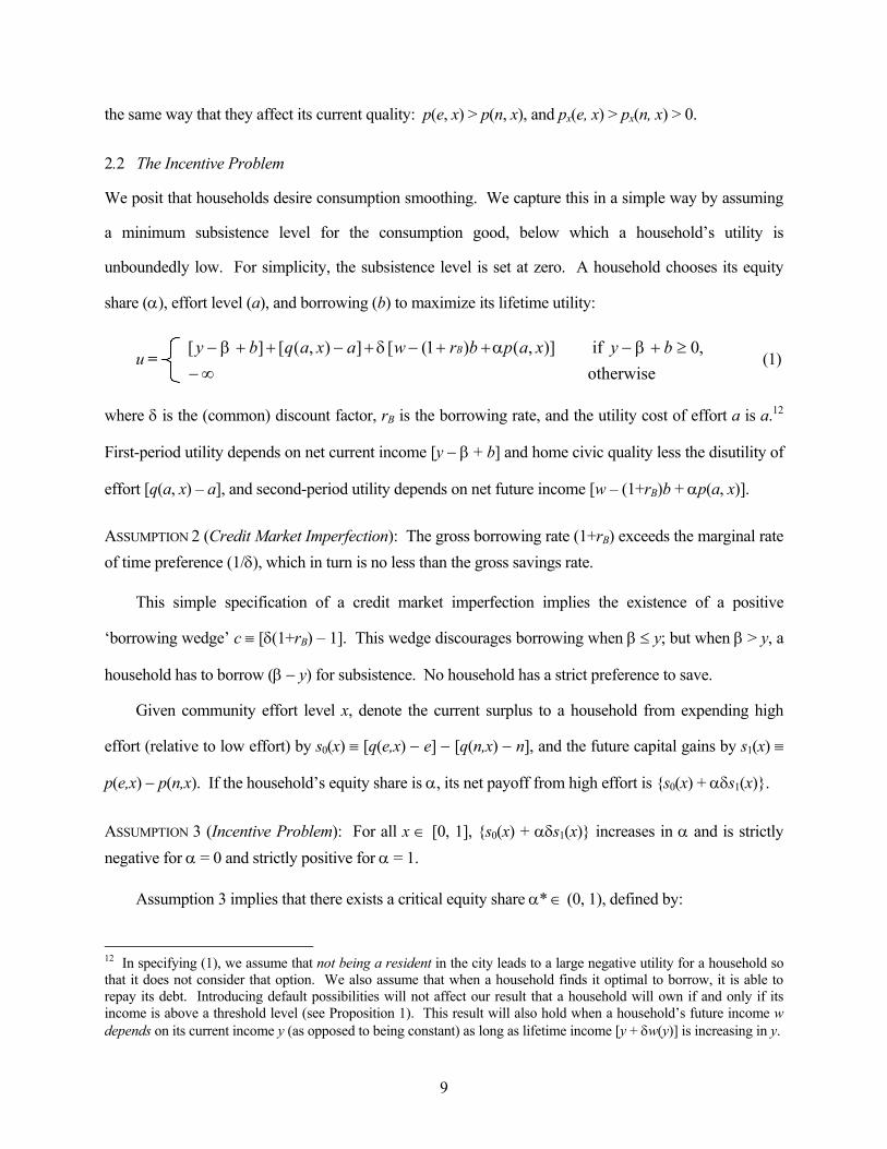
share (α), effort level (a), and borrowing (b) to maximize its lifetime utility:

u = (1) otherwise

,0 if )],()1([]),([][ ∞−

≥+−++−+−++− byxapbrwaxaqby B βαδβ

where δ is the (common) discount factor, rB is the borrowing rate, and the utility cost of effort a is a.12

First-period utility depends on net current income [y − β + b] and home civic quality less the disutility of

effort [q(a, x) – a], and second-period utility depends on net future income [w – (1+rB)b + αp(a, x)].

ASSUMPTION 2 (Credit Market Imperfection): The gross borrowing rate (1+rB) exceeds the marginal rate of time preference (1/δ), which in turn is no less than the gross savings rate.

This simple specification of a credit market imperfection implies the existence of a positive

‘borrowing wedge’ c ≡ [δ(1+rB) – 1]. This wedge discourages borrowing when β ≤ y; but when β > y, a

household has to borrow (β − y) for subsistence. No household has a strict preference to save.

Given community effort level x, denote the current surplus to a household from expending high

effort (relative to low effort) by s0(x) ≡ [q(e,x) − e] − [q(n,x) − n], and the future capital gains by s1(x) ≡

p(e,x) − p(n,x). If the household’s equity share is α, its net payoff from high effort is {s0(x) + αδs1(x)}.

ASSUMPTION 3 (Incentive Problem): For all x ∈ [0, 1], {s0(x) + αδs1(x)} increases in α and is strictly negative for α = 0 and strictly positive for α = 1.

Assumption 3 implies that there exists a critical equity share α* ∈ (0, 1), defined by:

12 In specifying (1), we assume that not being a resident in the city leads to a large negative utility for a household so that it does not consider that option. We also assume that when a household finds it optimal to borrow, it is able to repay its debt. Introducing default possibilities will not affect our result that a household will own if and only if its income is above a threshold level (see Proposition 1). This result will also hold when a household’s future income w depends on its current income y (as opposed to being constant) as long as lifetime income [y + δw(y)] is increasing in y.

9

)()(

)(*1

0

xsxs

xδ

α−

= , (2)

such that a household will expend high effort if and only if its home equity share is no less than α*.

In the next section, we determine a household’s optimal tenure choice. We show that the incentive

problem leads to a situation where the rich buy enough home equity so as to have the incentive to

expend high effort, while the poor do not. This moral hazard problem arises due to the non-

contractibility of effort (which is assumed to be unobservable to real estate companies), the households’

desire to smooth consumption, and the borrowing wedge. In Appendix I, we present a more general

agency model of tenure contracting and demonstrate the robustness of this result.

3. Tenure Choice

Consider a household residing in a community where the rental rate is ρ and the community effort level

is x. As the household is atomistic, it takes {x, ρ} as given. We model contract negotiation between the

household and a real estate company as follows: The household selects its home under the ‘default’

rental contract {0, ρ}. It can then renegotiate to a positive-equity contract {α > 0, β > ρ}. The price β of

equity share α is determined by a take-it-or-leave-it offer by the household to the real estate company,

with the status quo point of no renegotiation.

Under the rental contract {0, ρ}, a household expends negligible effort and receives utility:

un(y, x, ρ) = [y − ρ] + [q(n, x) − n] + δw, (3)

and the present value of the home is [ρ + δp(n, x)]. If the household renegotiates to buy equity share α, it

has to pay a price β(α| x,ρ) that is defined by: ρ + δp(n, x) = β(α| x,ρ) + δ(1−α)p(a0(α, x), x). The RHS

is the present value payoff to the real estate company under {α, β} given the household’s ‘sequentially

optimal’ effort a0(α, x) which equals e (resp., n) if α ≥ (resp. <) α*(x).

Let β*(x, ρ) ≡ β(α = α*(x)| x, ρ) denote the price of the critical equity share α*(x). Then:

β*(x, ρ) = ρ + α*(x)δp(n, x) − S(x), (4)

where S(x) ≡ s0(x) + δs1(x) is the ‘total surplus’ from high effort. The logic behind (4) is as follows: For

10

a household expending negligible effort, a real estate company will charge [ρ + α*δp(n,x)] for equity

share α*. But once a household buys α* both parties realize that it will put in high effort, and that leads

to the discount S(x) = s0(x) + α*δs1(x) + [1−α*]δs1(x), where s0(x) is the current cost of high effort and

α*δs1(x) is the minimal incentive payment required to elicit that effort. The remaining surplus

[1−α*]δs1(x) goes to the household as it has all the bargaining power in renegotiation.13

We refer to β*(x, ρ) as the ‘price of homeownership’: if a household invests this amount in home

equity, it obtains a large enough share of the capital gains to have the incentive to expend high effort.14

We will call a household that invests at least β* in home equity a ‘homeowner,’ and one that does not a

‘renter.’ Figure 1 depicts the set of available contracts {α, β} in community {x, ρ}.

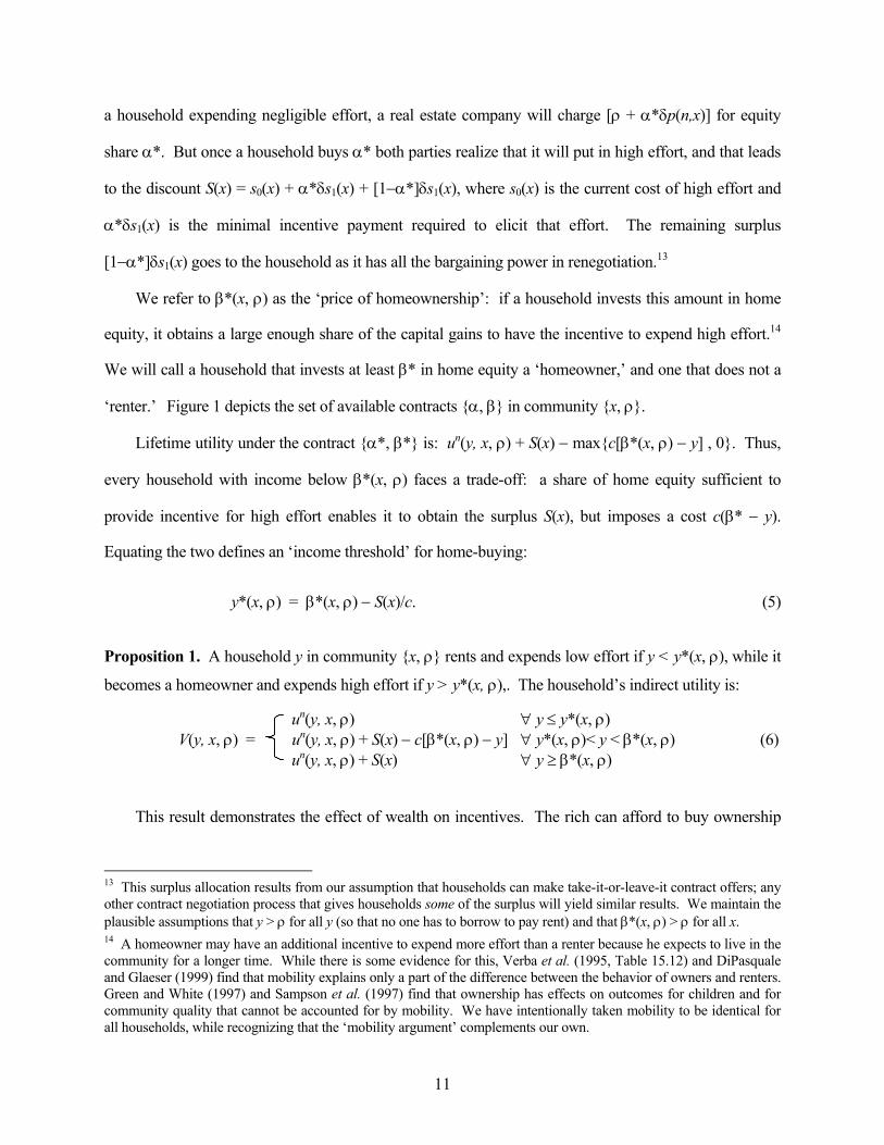
Lifetime utility under the contract {α*, β*} is: un(y, x, ρ) + S(x) − max{c[β*(x, ρ) − y] , 0}. Thus,

every household with income below β*(x, ρ) faces a trade-off: a share of home equity sufficient to

provide incentive for high effort enables it to obtain the surplus S(x), but imposes a cost c(β* − y).

Equating the two defines an ‘income threshold’ for home-buying:

y*(x, ρ) = β*(x, ρ) − S(x)/c. (5)

Proposition 1. A household y in community {x, ρ} rents and expends low effort if y < y*(x, ρ), while it

becomes a homeowner and expends high effort if y > y*(x, ρ),. The household’s indirect utility is:

un(y, x, ρ) ∀ y ≤ y*(x, ρ) V(y, x, ρ) = un(y, x, ρ) + S(x) − c[β*(x, ρ) − y] ∀ y*(x, ρ)< y < β*(x, ρ) (6) un(y, x, ρ) + S(x) ∀ y ≥ β*(x, ρ)

This result demonstrates the effect of wealth on incentives. The rich can afford to buy ownership

13 This surplus allocation results from our assumption that households can make take-it-or-leave-it contract offers; any other contract negotiation process that gives households some of the surplus will yield similar results. We maintain the plausible assumptions that y > ρ for all y (so that no one has to borrow to pay rent) and that β*(x, ρ) > ρ for all x. 14 A homeowner may have an additional incentive to expend more effort than a renter because he expects to live in the community for a longer time. While there is some evidence for this, Verba et al. (1995, Table 15.12) and DiPasquale and Glaeser (1999) find that mobility explains only a part of the difference between the behavior of owners and renters. Green and White (1997) and Sampson et al. (1997) find that ownership has effects on outcomes for children and for community quality that cannot be accounted for by mobility. We have intentionally taken mobility to be identical for all households, while recognizing that the ‘mobility argument’ complements our own.

11

contracts while the poor are stuck with rental contracts. As the former contracts impart greater residual

claim, the rich homeowners ‘solve’ the incentive problem and expend greater civic effort than renters.

However, that is only a part of our story. The magnitude of a household’s incentive problem

depends not only on its income, but also on community characteristics {x, ρ}. By the complementarity

effect, α* is a decreasing function of x. Further, when that effect is strong relative to the spillover effect,

the income threshold y* is also a decreasing function of x. Then the following condition holds:

Decreasing Threshold Condition (DT): yx*(x, ρ) < 0 ∀ x.15

Under DT, all residents in a community are better off with an increase in x (for a fixed ρ), and

homeowners gain more than renters: Vx(⋅)|y > y* > Vx(⋅)|y < y* > 0. Next, consider the marginal rate of

substitution between community effort and rent (MRSx,ρ) for the three types of households: renters,

‘mortgagees’ (i.e., homeowners that borrow), and self-financed owners. From (5) and (6), we have:

For renters: ),(* xnqdxd

xconstVyy =<

ρ

(7a)

For mortgagees: cxcyxnq

dxd xx

constVyy +

−=<< 1

),(),( *

**ρρ

β (7b)

For self-financed owners: )('),(* xSxnqdxd

xconstV

y +=<βρ

(7c)

All homeowners, because they obtain the surplus S(x), ‘take out’ more from a community than

renters. But mortgagees have a higher marginal cost of funds than the others. So, while MRSx,ρ is

always greater for self-financed owners than renters ((7c) > (7a)), that is not necessarily the case

between mortgagees and renters. To have (7b) > (7a) we need the following condition:

Single Crossing in Tenure (SCT): − yx*(x, ρ) > qx(n, x) ∀ x.

The SCT condition (which subsumes DT) holds when the complementarity effect is sufficiently

15 Note that dα*/dx = −α*(x){[(s0′(x)/−s0(x)] + [s1′(x)/s1(x)]}, which is strictly negative since s0(.) and s1(.) are strictly increasing in x by Assumption 1(ii). From (5), yx*(x, ρ) = δp(n, x)(dα*/dx) − (1+c/c)S′(x) + α*(x)δpx(n, x), where the first two terms are negative by the complementarity effect, and the last term is positive by the spillover effect.

12

stronger than the spillover effect.16 Then the indifference curves of owners and renters satisfy ‘single

crossing’: homeowners have a higher marginal willingness-to-pay for community effort than renters.

But SCT does not guarantee that a richer household is always willing to pay more for an increase in x.

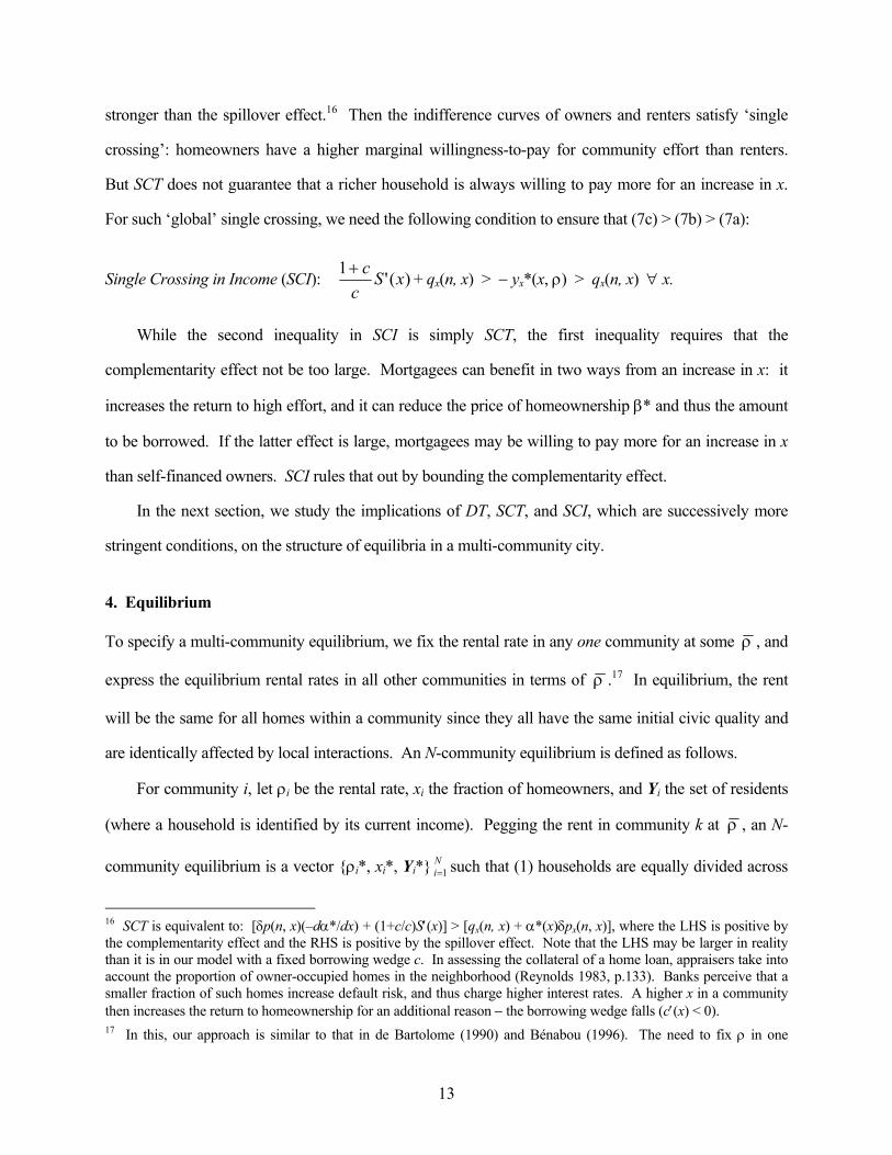
For such ‘global’ single crossing, we need the following condition to ensure that (7c) > (7b) > (7a):

Single Crossing in Income (SCI): )('1 xSc

c++ qx(n, x) > − yx*(x, ρ) > qx(n, x) ∀ x.

While the second inequality in SCI is simply SCT, the first inequality requires that the

complementarity effect not be too large. Mortgagees can benefit in two ways from an increase in x: it

increases the return to high effort, and it can reduce the price of homeownership β* and thus the amount

to be borrowed. If the latter effect is large, mortgagees may be willing to pay more for an increase in x

than self-financed owners. SCI rules that out by bounding the complementarity effect.

In the next section, we study the implications of DT, SCT, and SCI, which are successively more

stringent conditions, on the structure of equilibria in a multi-community city.

4. Equilibrium

To specify a multi-community equilibrium, we fix the rental rate in any one community at some ρ , and

express the equilibrium rental rates in all other communities in terms of ρ .17 In equilibrium, the rent

will be the same for all homes within a community since they all have the same initial civic quality and

are identically affected by local interactions. An N-community equilibrium is defined as follows.

For community i, let ρi be the rental rate, xi the fraction of homeowners, and Yi the set of residents

(where a household is identified by its current income). Pegging the rent in community k at ρ , an N-

community equilibrium is a vector {ρi*, xi*, Yi*} i such that (1) households are equally divided across N1=

16 SCT is equivalent to: [δp(n, x)(–dα*/dx) + (1+c/c)S′(x)] > [qx(n, x) + α*(x)δpx(n, x)], where the LHS is positive by the complementarity effect and the RHS is positive by the spillover effect. Note that the LHS may be larger in reality than it is in our model with a fixed borrowing wedge c. In assessing the collateral of a home loan, appraisers take into account the proportion of owner-occupied homes in the neighborhood (Reynolds 1983, p.133). Banks perceive that a smaller fraction of such homes increase default risk, and thus charge higher interest rates. A higher x in a community then increases the return to homeownership for an additional reason − the borrowing wedge falls (c′(x) < 0). 17 In this, our approach is similar to that in de Bartolome (1990) and Bénabou (1996). The need to fix ρ in one

13

the communities, (2) no household wants to relocate: V(y, xi*, ρi*) ≥ V(y, xj*, ρj*) for all y ∈ Yi*, for all

i and for all j ≠ i, and (3) there is ‘within-community equilibrium’ in every community.

A within-community equilibrium is described by the fraction of homeowners in the community, or

equivalently, by the community effort level. Consider any community i with its set of residents Yi. Let

Fi be the truncation of the income distribution function F on Yi. Given ρi and Fi, community effort xi

maps to a unique income threshold y*(xi, ρi) and thus to a set of residents who want to own. Then xi* is

a within-community equilibrium if and only if limity ↑ y*(⋅)Fi(y) ≤ 1 – xi* ≤ Fi(y*( xi, ρi)).18

4.1 Global Interactions Benchmark

Consider the following benchmark scenario. Instead of assuming that interaction effects are contained

within a community, suppose that these effects are city-wide. Then each household cares only about the

total number of city residents who expend high effort. Given F and ρ , define the set X* = {x ∈ [0,1]

limity ↑ y*(⋅) F(y) ≤ 1 − x ≤ F(y*(x, ρ ))}. Then {ρi*, xi*, Yi*} i is a ‘global interactions equilibrium’ if

and only if ρi*=

N1=

ρ for all i, Σ(xi*/N) ∈ X*, and the measure of Yi* is 1/N for all i.

Under global interactions, when the DT condition holds, household tenure choices cause a direct

externality for all other city residents − when some households switch from renting to owning, that

brings down the income threshold y* and encourages others to switch. This social multiplier effect can

generate multiple equilibria.19 Further, since Vx(.) > 0 under DT, the multiple equilibria are Pareto-

ranked: An equilibrium with a larger number of homeowners in the city Pareto-dominates one with a

smaller number. Thus, there exists a coordination problem in tenure choice.

In effect, the above analysis shows that if households are not allowed to move across communities,

then within a community, homeowners will be better citizens than renters, and a ceteris paribus increase

community arises from the fact that the aggregate demand and supply curves for homes in the city are vertical at unity. 18 The equilibrium condition allows for an atom in Fi at y*(xi, ρi): the largest measure of renters are all households with y ≤ y*(xi, ρi) (the first inequality), and all households with y > y*(xi, ρi) are homeowners (the second inequality). Standard fixed-point results guarantee the existence of an equilibrium xi* for any ρi and Fi. 19 To see this, suppose that F is continuous. Then an equilibrium x* ∈ X* is given by the intersection of the curves: y = y*(x, ρ ) and y = F−1(1−x). When these curves are downward sloping in the (x, y) space, they can have multiple intersections, and so X* can contain multiple elements. There can be multiple equilibria whenever y*x < 0 for some x.

14

in the homeownership rate will improve the welfare of all residents. But households are free to locate in

the community of their choice. When interaction effects are local, this has important consequences for

the equilibrium tenure distribution in a city and community outcomes. This is what we now turn to.

4.2 Local Interactions Equilibria

Under local interaction effects, there exist symmetric equilibria that are N-fold replications of global

interactions equilibria. Specifically, there exists a local interactions equilibrium with ρi* = ρ and xi*=

x* for all i if and only if x*∈ X*. Here, every community is a mirror-image of every other.

However, symmetric equilibria need not be ‘stable.’ Our notion of stability is analogous to that in

the multi-communities literature (see e.g., Fernandez 2001, p.7): an equilibrium is stable if, starting

from it, the relocation of a small mass of households from one community to another implies that under

the new outcomes within these communities, the relocated households prefer to return to the original

communities. [See Appendix II for a formal definition, and for the proofs of Propositions 2−5.]

Proposition 2. If DT holds, then an N-community equilibrium in which there exist two communities i and j with 0 < xi*= xj* < 1 is not stable.

Proposition 2 says that under a decreasing income threshold, a stable equilibrium under local

interactions must either have all owners (xi*=1 ∀ i) or all renters (xi*=0 ∀ i), or be asymmetric. Our

next result shows that if the complementarity effect is strong enough so that SCT holds (subsuming DT),

the asymmetry in tenure distribution in an N-community city must take a very particular form.

Proposition 3. If SCT holds, then all stable equilibria exhibit tenure segregation, where homeowners and renters co-reside in at most one community. For any pair {i, j} with xi* > xj*, the rental rate is

higher in community i, and if xj* > 0, the price of homeownership β* is also higher in community i.20

Complementarity in individual effort raises homeowners’ marginal willingness-to-pay for an

increase in community effort vis-à-vis renters’. Whenever the former exceeds the latter, even by an

If y*x > 0 for all x, then X* is a singleton set. Non-emptiness of X* is proved by standard fixed-point arguments. 20 It is also true that every tenure-segregated equilibrium in which no resident is indifferent between renting and owning within a community, is stable under SCT (the proof is available from the authors). On the other hand, if SCT

15

infinitesimal amount (that is all that SCT requires), there will be a stable agglomeration of home-

ownership, and homeowner communities will have higher property values than renter communities.

We presented evidence of tenure segregation in the US in Section 1.2. Communities in the US are

also segregated by income (see Jargowsky, 1997)). Can the two phenomena be related? Our next result

presents a sufficient condition for ‘complete segregation’, i.e., segregation by tenure and income.

Proposition 4. Suppose that SCI holds and that there exists a stable N-community equilibrium.21 Then there exists an equilibrium that is tenure-segregated and income-segregated: for any pair {i, j}, if xi* > xj* then all residents in community i are richer than those in community j.

When the global single crossing condition SCI holds, households segregate themselves by income

solely due to the relation between income and tenure choice.22 While there is a close link between the

forces that lead to tenure- and income-segregation, these forces are not identical. If mortgagees benefit

more from an increase in community effort than self-financed owners (i.e., if SCT holds but SCI does

not), then there can be an equilibrium that is segregated by tenure but not by income − where all middle-

class mortgagees come together in one community, and rich homeowners co-reside with poor renters in

another (an example is available from the authors). The general point is that when interaction effects

exist with respect to endogenous actions, the condition for segregation of agents who choose different

actions can be distinct from the condition for segregation of agents who differ in their types.

Under local interaction effects, the direct externality of tenure choice, identified in the global

interactions model, leads to a within-community social multiplier effect and can generate multiple

equilibria. We explore this issue with the help of an example, presented in Appendix III, of a two-

community city with ‘rich’, ‘middle class’, and ‘poor’ households. Figure 2 depicts three completely

segregated outcomes: the rich own homes in community 1, the poor rent in community 2, and the

middle class are ‘boundary agents’ indifferent between living in either community. In outcome A (resp.,

does not hold, there can exist stable equilibria that are not tenure-segregated (an example is available from the authors). 21 Regarding existence, we have the following result (proof available from the authors): If income is continuously distributed on [y−, y+], and if SCI holds, then there exists a stable equilibrium that is completely segregated. But a continuous income distribution is not necessary for existence; see our ‘discrete’ example in Appendix III. 22 There will obviously be additional reasons for income segregation when publicly provided goods like schools are locally financed (see, for example, Fernandez and Rogerson 1996, Bénabou 1996, and Durlauf 1996).

16

C), all middle class households are indifferent between renting (resp., owning) in either community,

while in outcome B they are indifferent between owning in community 1 and renting in community 2.

In our example, when the middle-class income is of intermediate value and there are ‘not too many’

rich and poor households, A, B, and C co-exist as stable equilibrium outcomes (see Result 1 in Appendix

III). Starting from A (resp., B), if enough middle class residents in community 1 (resp., community 2)

make a tenure switch, then all of them will do so, and B (resp., C) will be reached.

However, in contrast to the global interactions case, the multiple equilibria are not necessarily

Pareto-ranked on the basis of the total number of homeowners in the city. This is due to a ‘fiscal

externality’ in the local interactions model − a relative increase in homeownership in a community raises

its relative rental rate. Then an equilibrium E′ can have more homeowners than another equilibrium E″

and the two can be Pareto-incomparable. In our example, a move from B to C leads to an increase in the

total number of homeowners, but also raises rents in community 2 so as to make homeowners indifferent

between the two communities. Under SCT, this leaves the poor renters worse off in C than in B as their

benefit from the improvement in community 2 civic quality is more than offset by the higher rent.

While relative rent changes can be unambiguously determined across different equilibria, absolute

changes in rents cannot be so determined as they depend on the posited ‘rent normalization’ (i.e., ρk =

ρ ).23 As a result, definitive predictions about utility changes of agents across equilibria cannot be made

since utility depends on absolute rent levels. We have, however, the following result:

Proposition 5. When SCI holds, let E′ and E″ be two completely segregated equilibria with community

i outcomes {xi′, ρi′} and {xi″, ρi″} respectively, with xi′ > xi″. If a community i resident has the same

utility in E′ and E″, then all households richer (resp., poorer) than that resident are better off in E′ (resp.,

E″). If ρi′ − ρi″ ≤ [q(n, xi′) − q(n, xi″)] then all community i residents are better off in E′, and if ρi′ − ρi″

≥ [q(n, xi′) − q(n, xi″)] + [S(xi′) − S(xi″)] then all community i residents are better off in E″.

In the next section, we use the above result to identify winners and losers from a housing subsidy

policy that expands homeownership, but affects property values in the process.

23 See the discussion following Proposition I in Appendix III. The ambiguity in absolute rent changes is not caused by rent normalization. With vertical demand and supply of homes, if we do not normalize rents, there will be infinitely

17

5. Inefficiency and Policy

Given a tenure profile x = {x1, x2, … xN}, it is natural to define ‘net community quality’ for any

community i as: Q(xi) ≡ xi[q(e, xi) + δp(e, xi) − e] + (1−xi)[q(n, xi) + δp(n, xi) − n], and ‘net city quality’

as Σ i Q(xN1= i). If net city quality is greater under a tenure profile x′ than under x″, the former is more

efficient in that, if the borrowing wedge c represents profits accruing to lenders, the sum of utilities of all

agents − all city residents, real estate companies, and lenders − will be higher under x′ than under x″.24

In our model, there can be under-investment in home-buying as homeowners are not compensated

for the positive externalities that they generate. This problem may be compounded by a coordination

failure in tenure choice. For these reasons, there may be too few homeowners in equilibrium.

Further, note that Q′′(x) = 2S′(x) + {xS″(x) + qxx(n, x) + δpxx(n, x)}. While the first term is positive

by the complementarity effect (this is what causes tenure segregation), the sign of the second bracketed

term depends on the curvature of q(.) and p(.). If these functions are sufficiently concave in x, Q(.) will

be strictly concave in x. Then equilibrium tenure segregation will be ‘distributionally’ inefficient, and

net city quality will be improved by equalizing ownership rates across communities.

5.1 Housing Subsidy Schemes

The possibility of under-investment in homeownership immediately suggests a role for housing

subsidies.25 Since Q′(x) = S(x) + xS′(x) + qx(n, x) + δpx(n, x), with all terms on the RHS strictly positive,

a subsidy policy that alters the city tenure profile from x′ to x″ in a way that the latter vector-dominates

the former, will lead to an increase in net city quality and so enhance efficiency.

Consider the following subsidy scheme. Starting from a pre-subsidy equilibrium, current home-

owners and real estate companies are taxed lump sum, and current renters receive a subsidy specifically

many rent vectors for each equilibrium tenure profile. Absolute rent changes across equilibria will still be ambiguous. 24 It is obviously restrictive to think of c just as lender profits since that implies that credit market imperfections arise solely out of imperfect competition among lenders. In reality, these imperfections may arise from more fundamental information asymmetries. Even if that is the case, the sum of utilities of all city residents and real estate companies can be higher under x′ than under x″ when Σ i Q(x′i) > Σ i Q(x″i).

N1=

N1=

25 Another way to alleviate the under-investment problem is to reduce the borrowing wedge c. We implicitly assume is that the underlying reasons for credit market imperfections cannot be changed by simple policy measures.

18

for home-buying. Subsidies can be ‘uniform’ (the same for all recipients) or ‘targeted’ (conditioned on

recipient income). If a policy maker with limited information about the magnitude of local interaction

effects and income distribution implements such a scheme, will the city tenure profile necessarily

improve? Will all households necessarily gain? Will it be cheaper to give targeted subsidies?

We address these questions using our two-community example. Starting from outcome A, we

determine what can be achieved by giving increasing levels of subsidies when SCI holds and when the

tax-burden on the rich is not so large that they switch to renting. We identify the following features of

housing subsidy policies. [See Results 1−3 in Appendix III and the discussion following them.]

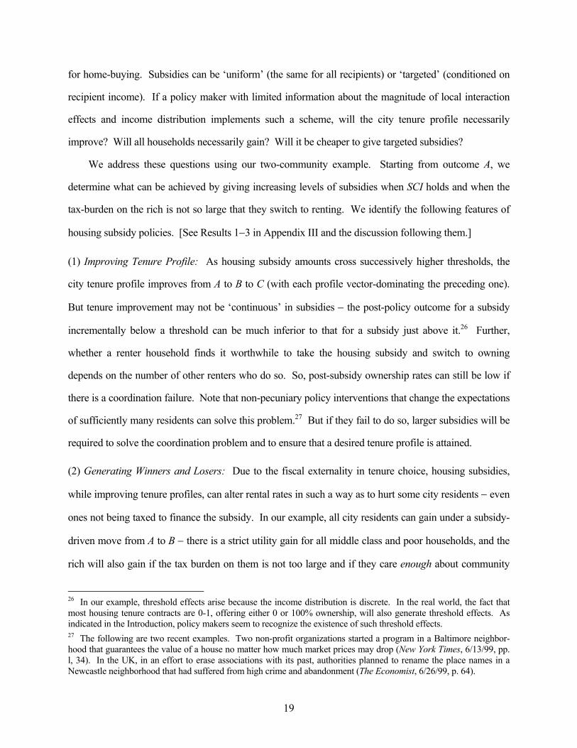
(1) Improving Tenure Profile: As housing subsidy amounts cross successively higher thresholds, the

city tenure profile improves from A to B to C (with each profile vector-dominating the preceding one).

But tenure improvement may not be ‘continuous’ in subsidies − the post-policy outcome for a subsidy

incrementally below a threshold can be much inferior to that for a subsidy just above it.26 Further,

whether a renter household finds it worthwhile to take the housing subsidy and switch to owning

depends on the number of other renters who do so. So, post-subsidy ownership rates can still be low if

there is a coordination failure. Note that non-pecuniary policy interventions that change the expectations

of sufficiently many residents can solve this problem.27 But if they fail to do so, larger subsidies will be

required to solve the coordination problem and to ensure that a desired tenure profile is attained.

(2) Generating Winners and Losers: Due to the fiscal externality in tenure choice, housing subsidies,

while improving tenure profiles, can alter rental rates in such a way as to hurt some city residents − even

ones not being taxed to finance the subsidy. In our example, all city residents can gain under a subsidy-

driven move from A to B − there is a strict utility gain for all middle class and poor households, and the

rich will also gain if the tax burden on them is not too large and if they care enough about community

26 In our example, threshold effects arise because the income distribution is discrete. In the real world, the fact that most housing tenure contracts are 0-1, offering either 0 or 100% ownership, will also generate threshold effects. As indicated in the Introduction, policy makers seem to recognize the existence of such threshold effects. 27 The following are two recent examples. Two non-profit organizations started a program in a Baltimore neighbor-hood that guarantees the value of a house no matter how much market prices may drop (New York Times, 6/13/99, pp. l, 34). In the UK, in an effort to erase associations with its past, authorities planned to rename the place names in a Newcastle neighborhood that had suffered from high crime and abandonment (The Economist, 6/26/99, p. 64).

19

quality. But if the subsidy level is increased further so that the city moves from B to C, the utility

changes are reversed − while the middle class neither gains nor loses from the move, the rich are worse

off because of the tax burden, and the poor are worse off because of the increase in rents.

Because of the fiscal externality, household utility can change non-monotonically with subsidy-

induced improvements in tenure profile. Without detailed knowledge of the ‘city parameters,’ it is not

possible to predict the precise welfare changes of city residents for any given level of subsidy. However,

Proposition 5 allows us to conclude that (apart from the welfare loss of the rich due to the tax burden):

(i) a subsidy-induced increase in property values in a community is most likely to hurt the poorest

residents, especially if they continue to rent in the post-subsidy equilibrium, and (ii) if the poorest

residents do not lose post-subsidy, then all community residents gain.

(3) Targeted Subsidies: If subsidies can be conditioned on recipients’ incomes, then a desired tenure

profile can be achieved at a lower cost. In our example, the ‘all owners {xi = 1 ∀ i}’ outcome can be

attained with a smaller aggregate subsidy bill under targeted subsidies than under uniform subsidies.

This is because a targeted subsidy scheme can utilize the within-community social multiplier. In our

example, the targeted subsidy policy pulls up the middle class into homeownership, and then gives the

minimal subsidy that is necessary to induce the poor to own as well. The scheme demonstrates that it

can be more effective to give a moderate subsidy to both middle- and low-income households than a

large one to the latter, even if the social objective function counts only the welfare of the latter.28

5.2 Desegregation Policies

When tenure segregation is inefficient, i.e., when net community quality is concave in community effort,

the aim of a corrective policy is to encourage homeowners to ‘accept’ renters as their community

neighbors. We now present a tax-subsidy scheme that can induce ‘stable desegregation.’

Let *x < 1 be the maximal element of X* (the set of global interactions equilibria), and suppose

that the tenure profile {xi = *x ∀ i} is more efficient than the ‘best’ asymmetric equilibrium tenure

28 The informational demands of targeted subsidies are more than those of a uniform subsidy scheme. To design the least-cost targeted subsidy scheme, a policy maker needs to know not only a recipient’s income class, but also the income threshold for home-buying for that income class.

20

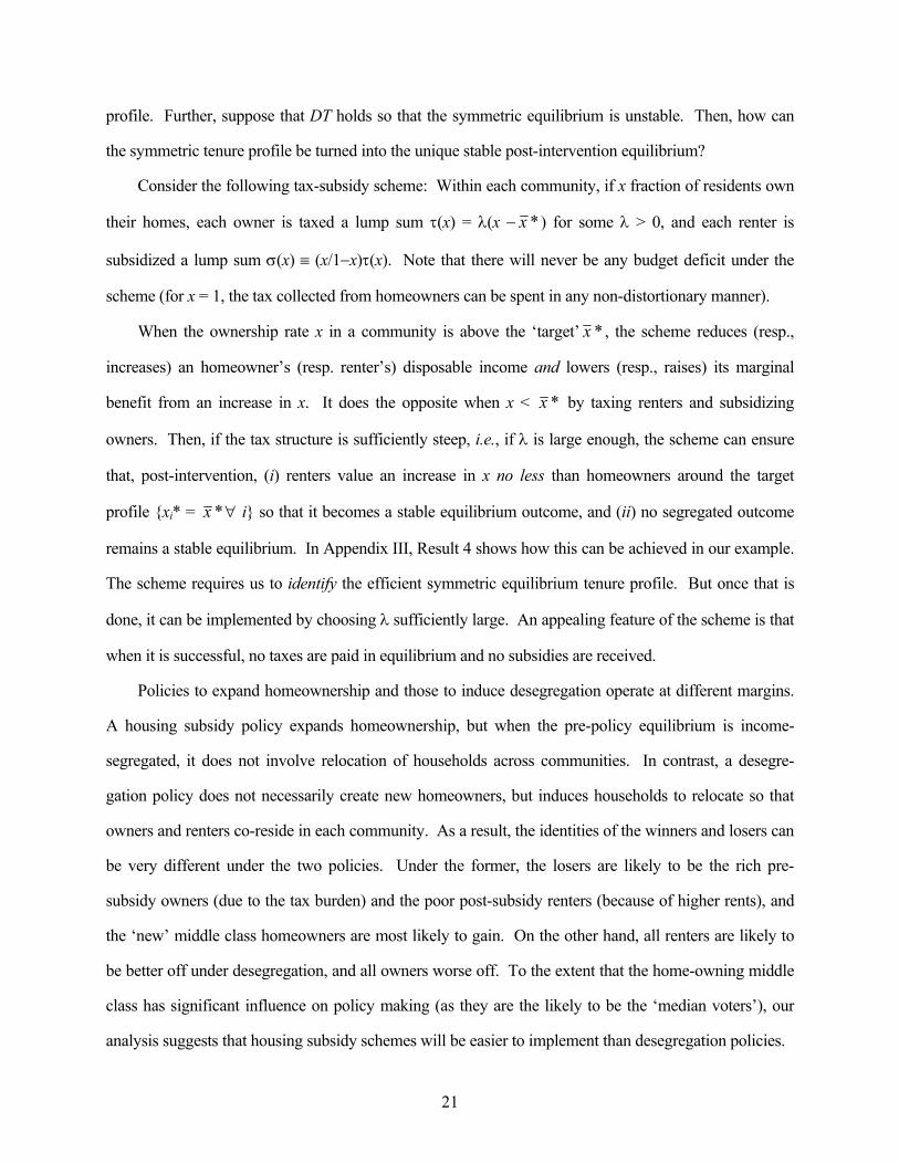
profile. Further, suppose that DT holds so that the symmetric equilibrium is unstable. Then, how can

the symmetric tenure profile be turned into the unique stable post-intervention equilibrium?

Consider the following tax-subsidy scheme: Within each community, if x fraction of residents own

their homes, each owner is taxed a lump sum τ(x) = λ(x − *x ) for some λ > 0, and each renter is

subsidized a lump sum σ(x) ≡ (x/1−x)τ(x). Note that there will never be any budget deficit under the

scheme (for x = 1, the tax collected from homeowners can be spent in any non-distortionary manner).

When the ownership rate x in a community is above the ‘target’ *x , the scheme reduces (resp.,

increases) an homeowner’s (resp. renter’s) disposable income and lowers (resp., raises) its marginal

benefit from an increase in x. It does the opposite when x < *x by taxing renters and subsidizing

owners. Then, if the tax structure is sufficiently steep, i.e., if λ is large enough, the scheme can ensure

that, post-intervention, (i) renters value an increase in x no less than homeowners around the target

profile {xi* = *x ∀ i} so that it becomes a stable equilibrium outcome, and (ii) no segregated outcome

remains a stable equilibrium. In Appendix III, Result 4 shows how this can be achieved in our example.

The scheme requires us to identify the efficient symmetric equilibrium tenure profile. But once that is

done, it can be implemented by choosing λ sufficiently large. An appealing feature of the scheme is that

when it is successful, no taxes are paid in equilibrium and no subsidies are received.

Policies to expand homeownership and those to induce desegregation operate at different margins.

A housing subsidy policy expands homeownership, but when the pre-policy equilibrium is income-

segregated, it does not involve relocation of households across communities. In contrast, a desegre-

gation policy does not necessarily create new homeowners, but induces households to relocate so that

owners and renters co-reside in each community. As a result, the identities of the winners and losers can

be very different under the two policies. Under the former, the losers are likely to be the rich pre-

subsidy owners (due to the tax burden) and the poor post-subsidy renters (because of higher rents), and

the ‘new’ middle class homeowners are most likely to gain. On the other hand, all renters are likely to

be better off under desegregation, and all owners worse off. To the extent that the home-owning middle

class has significant influence on policy making (as they are the likely to be the ‘median voters’), our

analysis suggests that housing subsidy schemes will be easier to implement than desegregation policies.

21

6. Conclusion

A key feature of a healthy community is that residents are proactive participants in community

institutions. This paper presents a community-interactions model where externalities arising from non-

contractible individual effort produce concentrations of low-income households in disadvantaged renter

communities in which residents lack the incentive to be proactive. In our model, all households desire to

be homeowners and be responsive citizens, but credit market imperfections force the poorer ones to rent.

All households also want to live near homeowners because they generate positive externalities. But

homeowners may outbid renters for land in communities with a high proportion of homeowners, leading

to tenure segregation. An interplay of within-community externalities and market forces can create

‘good’ and ‘bad’ citizens out of ex ante similar households and then clump each group together.

Our analysis explains the significant segregation of homeowners and renters across communities in

the US, and the fact that poor renter communities have much worse civic environments than rich

homeowner communities. The model also provides a framework to study policy intervention in the

housing market. We show how different tax-subsidy schemes can improve the city tenure profile and

induce co-residence of owners and renters. By determining the winners and losers under alternative tax-

subsidy policies, we identify the sources of potential political opposition to such policies.

A limitation of our work is that it is essentially static. In the real world, the process of spatial

arbitrage that we treat as instantaneous, plays out over time. Intertemporally, community interaction

effects have the potential of magnifying small changes in individual behavior and thus generating large

changes in aggregate community quality. Then a small policy intervention can achieve remarkable

results in improving a neighborhood.29 However, our framework does provide a useful starting point for

a dynamic analysis of the impact of a government-sponsored homeownership program on the time path

of housing prices, homeownership rates, and improvements in community civic environment.

29 An example of this is the turn-around of Charlotte Gardens in the South Bronx that is referred to in the New York Times editorial quoted at the beginning of our paper. In the 1970’s, the South Bronx was “the definition of blight, nearly destroyed by poverty, crime, and arson” (New York Times, 11/2/1997). With money from New York City, 89 single-family homes were built in Charlotte Gardens in the mid-1980’s, and sold for $49,500-$60,000 to low-income families who agreed not to sell their homes for ten years. Mayor Ed Koch pronounced that the new owners would “defend these houses with their lives.” By 1997, their value had risen to $185,000, private construction had increased, and property values had risen all over the South Bronx.

22

Appendix I: An Agency Model of Tenure Contracting

The contracting model presented in the text contains two critical simplifying assumptions: (i) tenure

contracts have to be linear in the observable outcome − the future price of a home, and (ii) this price is a

deterministic function of unobservable effort. In what follows, we briefly present a more general

principal-agent model of tenure contracting between a household and a real estate company.

A long-lived risk-neutral principal (real estate company) owns a durable good H (housing unit). An

agent (household) lives for two periods and benefits from consuming the flow of services from H only in

the first period. In that period, the agent can put in effort to add value to H, which benefits her and

increases the future price of H (this price goes to the principal). Both players consume a divisible

numeraire commodity in all periods, and discount the future by δ ∈ (0, 1).

The agent’s effort (a) can be high (e) or low (n). It is not observable by the principal and so cannot

be contracted upon. The agent’s current benefit from effort net of cost is [q(a) − a]. The future price of

H is a random variable P distributed on [0, ∞) according to G(p|a), where G(p|e) first-order

stochastically dominates G(p|n). A feasible contract is a pair {α(p), β}, where β ∈ ℜ is the ‘up-front

payment’ that the agent makes to the principal, and α(p) is the ‘rebate’ that the principal gives back to

the agent in the second period if the realized future price of H is p. The rebate function α(p) can be any

real-valued function, but it is required to satisfy the ‘limited liability clause’ α(p) ≥ 0 for all p. The

contract {α, β} is thus a specific ‘complete contract with limited liability’ under moral hazard.

Given {α, β}, if the agent (with current income y and future income w) chooses effort a and

borrows b, the principal’s utility is π(a;α,β) = β + δ ∫ , and the agent’s utility is: )|()]([0

apdGpp∞

−α

u(a, b; α, β | y) =

otherwise,

,0 if )|()]()1([])([][ 0

∞−

≥+−++−+−++− ∫∞

byapdGpbrwaaqby B βαδβ

where the borrowing wedge [δ(1+rB) − 1] is strictly positive.

Let effort level α*(β, α| y) and debt level b*(β, α| y) maximize u(⋅| y) under the contract {α, β}.

Assume the existence of the following incentive problem: (i) if α(p) = 0 for all p, then α* = n for all y,

and (ii) if α(p) = p for all p, then α* = e for all y. Assume further that the players have the right to the

default rental contract {α(p) = 0 ∀ p, β = ρ}. This contract pins down the players’ reservation payoffs:

23

for the principal, π0 = ρ + δ ; and for the agent, u)|(0

npdGp∫∞ 0(y) = [y − ρ] + [q(n) − n] + δw.

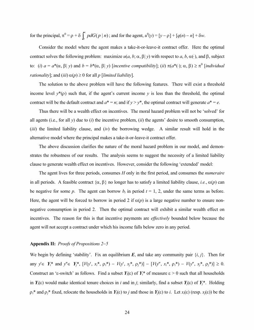
Consider the model where the agent makes a take-it-or-leave-it contract offer. Here the optimal

contract solves the following problem: maximize u(a, b; α, β| y) with respect to a, b, α(⋅), and β, subject

to: (i) a = a*(α, β| y) and b = b*(α, β| y) [incentive compatibility]; (ii) π(a*(⋅); α, β) ≥ π0 [individual

rationality]; and (iii) α(p) ≥ 0 for all p [limited liability].

The solution to the above problem will have the following features. There will exist a threshold

income level y*(ρ) such that, if the agent’s current income y is less than the threshold, the optimal

contract will be the default contract and a* = n; and if y > y*, the optimal contract will generate a* = e.

Thus there will be a wealth effect on incentives. The moral hazard problem will not be ‘solved’ for

all agents (i.e., for all y) due to (i) the incentive problem, (ii) the agents’ desire to smooth consumption,

(iii) the limited liability clause, and (iv) the borrowing wedge. A similar result will hold in the

alternative model where the principal makes a take-it-or-leave-it contract offer.

The above discussion clarifies the nature of the moral hazard problem in our model, and demon-

strates the robustness of our results. The analysis seems to suggest the necessity of a limited liability

clause to generate wealth effect on incentives. However, consider the following ‘extended’ model:

The agent lives for three periods, consumes H only in the first period, and consumes the numeraire

in all periods. A feasible contract {α, β} no longer has to satisfy a limited liability clause, i.e., α(p) can

be negative for some p. The agent can borrow bt in period t = 1, 2, under the same terms as before.

Here, the agent will be forced to borrow in period 2 if α(p) is a large negative number to ensure non-

negative consumption in period 2. Then the optimal contract will exhibit a similar wealth effect on

incentives. The reason for this is that incentive payments are effectively bounded below because the

agent will not accept a contract under which his income falls below zero in any period.

Appendix II: Proofs of Propositions 2−5

We begin by defining ‘stability’. Fix an equilibrium E, and take any community pair {i, j}. Then for

any y′∈ Yi* and y″∈ Yj*, [V(y′, xi*, ρi*) − V(y′, xj*, ρj*)] − [V(y″, xi*, ρi*) − V(y″, xj*, ρj*)] ≥ 0.

Construct an ‘ε-switch’ as follows. Find a subset Yi(ε) of Yi* of measure ε > 0 such that all households

in Yi(ε) would make identical tenure choices in i and in j; similarly, find a subset Yj(ε) of Yj*. Holding

ρi* and ρj* fixed, relocate the households in Yi(ε) to j and those in Yj(ε) to i. Let xi(ε) (resp. xj(ε)) be the

24

post-switch tenure outcome in i (resp., j) when all old residents in i (resp., j) make the same tenure

choice as before and the migrants in i (resp., j) respond optimally to (xi*, ρi*) (resp., (xj*, ρj*)). If the

condition: [V(y′, xi(ε), ρi*) − V(y′, xj(ε), ρj*)] − [V(y″, xi(ε), ρi*) − V(y″, xj(ε), ρj*)] ≥ 0 for all y′∈ Yi(ε)

and y″∈ Yj(ε), holds for all ε-switches for ε small, and for all {i, j}, then E is (locally) stable.30

Next, we establish the following claim that is used in our proofs. To simplify the notation, let yi* ≡

y*(xi*, ρi*), βi* ≡ β*(xi*, ρi*), qi* ≡ q(n, xi*), and Si* ≡ S(xi*). From (5) and (6), note that Vi(y) = un(y, xi,

ρi) for y ≤ y*(xi, ρi), and Vi(y) = un(y, xi, ρi) + min{c(y− y*(xi, ρi)), S(xi)} for y > y*(xi, ρi).

Claim. (a) When SCT holds, if xi* > xj* and ρi* − ρj* ≤ qi* − qj*, then yi* < yj*.

(b) When SCI holds, if xi* > xj* and ρi*−ρj* ≥ (qi* − qj*) + (Si* − Sj*), then βi* > βj*.

Proof: Note that yj* − yi* = −[ y(xi*, ρj*)−yj*] − [ρi*−ρj*] = [−y*∫*

*

i

j

x

xx(x, ρj*)]dx − [ρi*−ρj*]. By SCT,

this is strictly greater than [qi*−qj*] − [ρi*−ρj*], proving (a). Part (b) is proved similarly.

Proof of Proposition 2: Consider an equilibrium where there is a community pair {i, j} with 0 < xi* =

xj* < 1. Then ρi* = ρj*, and so yi* = yj*. Consider an ε-switch as described above where y′ > yi* = yj* >

y″ for all y′∈ Yi(ε) and y″∈ Yj(ε). After the switch, the migrants to i (resp., j) will rent (resp., own)

implying that xi(ε) < xi* = xj* < xj(ε). Then [V(y′, xi(ε), ρi*) − V(y′, xj(ε), ρj*)] − [V(y″, xi(ε), ρi*) − V(y″,

xj(ε), ρj*)] = − , which is strictly negative under DT for any y′∈

Y

∫ ′′−′)(

)(*)],,(*),,([

ε

ερρ

j

i

x

xixix dxxyVxyV

i(ε) and y″∈ Yj(ε) and ε > 0. Thus an equilibrium with 0 < xi* = xj* < 1 is unstable under DT.

Proof of Proposition 3: Suppose that E is a stable equilibrium that is not tenure-segregated. Then there

is a pair {i, j} with xi*∈ (0, 1) and xj*∈ (0, 1). Since SCT subsumes DT, stability implies that xi* ≠ xj*.

Suppose (w.l.o.g.) that 1 > xi* > xj* > 0. Since there are renters in i and in j, ρi* − ρj* = qi* − qj*. Then

yi* < yj* by Claim (a). This implies that for all y ∈ (yi*, yj*], Vi(y) > un(y, xi*, ρi*) = un(y, xj*, ρj*) =

Vj(y), and that for all y > yj*, Vi(y) = un(y, xi*, ρi*) + min{c(y – yi*), Si*} > un(y, xj*, ρj*) + min{c(y –

30 If there were a finite number of households, we would check for stability by relocating one household, and it would obviously make a unique tenure choice in a community. That is why we require all households in Yi(ε) to make identical tenure choices in i and in j. Further, instead of using xi(ε), we could work with xi*(ε) where xi*(ε) is a post-switch equilibrium in i given ρi*. For any given ε-switch, whether the inequality required for stability holds or not depends on the signs of [xi*(ε) − xi*] and [xj*(ε) − xj*]. If xl*(ε) is unique for l = i, j, then [xl*(ε) − xl*] will have the same sign as [xl(ε) − xl*], and so the two definitions will give the same results. Even if there are multiple post-switch equilibria, there will be at least one equilibrium in each community l where [xl*(ε)−xl*] has the same sign as [xl(ε)−xl*].

25

yj*), Sj*} = Vj(y). So, all households with income y > yi* strictly prefer to live in i (and own). Then there

can be no owners in j, contradicting our supposition that xj* > 0. So E must be tenure segregated.

Regarding housing prices in the two communities, xi* > xj* implies that ρi* > ρj*, since otherwise

the renters in j will move to i. When xj* > 0, it must be that yi* ≥ yj*, since otherwise there can be no

owners in j. By (5), xi* > xj* and yi* ≥ yj* implies that βi* > βj*, and Proposition 3 is established.

Proof of Proposition 4: Let E be a stable equilibrium, and take any {i, j} in E with xi* > xj*. Since SCI

subsumes SCT, E is tenure segregated. Then there are three cases: (i) 1 = xi* > xj* = 0, (ii) 1 > xi* > xj*

= 0, and (iii) 1 = xi* > xj* > 0. In case (i), suppose that y′ > y′′ and that y′ lives in j and y′′ in i. Then y′

must prefer to rent in j than own in i, and y′′ must prefer to own in i than rent in j, i.e., min{c(y′′−yi*),

Si*} ≥ (ρi* − ρj*) − (qi* − qj*) ≥ min{c(y′−yi*), Si*}. This inequality can be satisfied if and only if y′′ ≥

βi*, and in that case, ρi* − ρj* = qi* − qj* + Si*. But then, βi* > βj* by SCI and Claim (b), which implies

that y′ > y′′ ≥ βi* > βj*. Then y′ strictly prefers to own in j which contradicts our supposition that xj* = 0.

Thus, when xi*= 1 and xj*= 0, residents in i are richer than those in j.

In case (ii), it must be that ρi* − ρj* = qi* − qj*, yi* < yj*, and all households with y > yi* strictly

prefer to live in i. So, if y′ > y′′, and y′ lives in j while y′′ lives in i, both must rent and so be indifferent

between i and j. In case (iii), it can be proved using similar arguments that for any y′ > y′′, either it

cannot be that y′ lives in j and y′′ lives in i, or it must be that y′ and y′′ are indifferent to living in i and j.

When they are indifferent, y′ can be moved to i and y′′ can be moved to j without disturbing any

equilirium conditions. So if a stable equilibrium exists, there must be one that is completely segregated.

Proof of Proposition 5: Since E′ and E″ are completely segregated, the set of residents in i (Yi*) is the

same in both. Our first claim follows directly from SCI. Consider the poorest resident in i, who

necessarily rents in E″. When ρi′−ρi″ ≤ [q(n, xi′)−q(n, xi″)], it is better off in E′ whether it rents or owns

in E′. Then all residents in i are better off in E′. Next, consider the richest resident in i, who necessarily

owns in E′. When ρi′−ρi″ ≥ [q(n, xi′)−q(n, xi″)] + [S(xi′)−S(xi″)], it is worse off in E′ whether it owns or

rents in E″ since β*(xi′, ρi′) > β*( xi″, ρi″) under SCI. Then all residents in i are worse off in E′.

Appendix III: An Example of a Two-community City

Consider a city with two communities, each with homes of measure half. There is µH measure of ‘rich’

26

households each with income yH, the ‘middle class’ is of measure µM each with income yM, and there is

µL measure of ‘poor’ households each with income yL (with µH+µM+µL = 1). We posit that the q(.) and

the p(.) functions are such that SCI holds. Community 1 rental rate is pegged at ρ .

Let *y ≡ y*(1, ρ ) and *β ≡ β*(1, ρ ). Define ρ0(y) ≡ ρ − [q(n,1)−q(n,0)]−c[y− *y ]. Under SCI,

there exists a unique y0∈ ( *y , y(0, ρ )) such that y0 = y*(0, ρ0(y0)). Let β0 ≡ β*(0, ρ0(y0)). Then, *y <

y0 < β0 < *β . Next, define µ such that y0 = y*(2µ , ρ ). Finally, define (µ) ≡ρ ρ − [q(n,1) −

q(n,1−2µ)] − c[y*(1−2µ, (µ)) −ρ *y ]. Note that for y∈ ( *y , y0), there exists a unique ∈ (0, ½)

such that y = y*(1−2µ , ( )).

)(ˆ yµ

) ρ(ˆ y )(ˆ yµ

We assume that (i) the rich always own and the poor always rent, (ii) the middle class income is the

median income, and (iii) if a middle class household ‘buys’ a home, it has to take out a mortgage:

Parameter restriction [R]: (i) yL < *y < y*(0, ρ ) < yH, (ii) µθ ∈ (0, ½) for θ = L, H, and (iii) yM < β0.

Supposing that x1 ≥ x2 (w.l.o.g.), A, B, and C are the only completely segregated outcomes under [R].

Result 1. Under [R] and the normalization ρ1 = ρ : (i) A is a stable equilibrium outcome if and only if

yM < y*(2µH, ); (ii) B is a stable equilibrium outcome if and only if < yM < y0; and (iii) C is a

stable equilibrium outcome if and only if either {y0 < yM} or { *y < yM < y0 and µL < }. )(ˆ yµ

*yρM

Proof: Let ρi(O) be the equilibrium rental rate in i in outcome O. (i) For A to be equilibrium, yM must

be indifferent between renting in 1 and in 2, requiring that ρ1(A) − ρ2(A) = [q(n, 2µH) − q(n, 0)]. Then yM

will strictly prefer to rent if and only if yM < y*(2µH, ρ ). Here and subsequently, strict preference is

required for stability. (ii) For B to be equilibrium, yM must be indifferent between being a mortgagee in

1 and renting in 2, requiring that ρ1(B) − ρ2(B) = [q(n, 1)−q(n, 0)] + c[yM − *y ]. Then yM will strictly

prefer to own in 1 if and only if yM > *y and to rent in 2 if and only if yM < y*(0, ρ2(B)) = y0. (iii) For C

to be equilibrium, yM must be indifferent between being a mortgagee in 1 and in 2, requiring that ρ1(B) −

ρ2(B) = [q(n, 1)−q(n, 0)] + c[y*(1−2µL, (µρ L)) − *y ]. Then yM will strictly prefer to own in 1 if and

only if yM > *y and to own in 2 if and only if yM > y*(1−2µL, (µρ L)). The last condition is satisfied if

and only if either {y0 < yM} or {yM < y0 and µL < }. )(ˆ Myµ

Result 1 shows that given ρ1 = ρ , A, B, and C co-exist as stable equilibria when, in addition to [R],

27

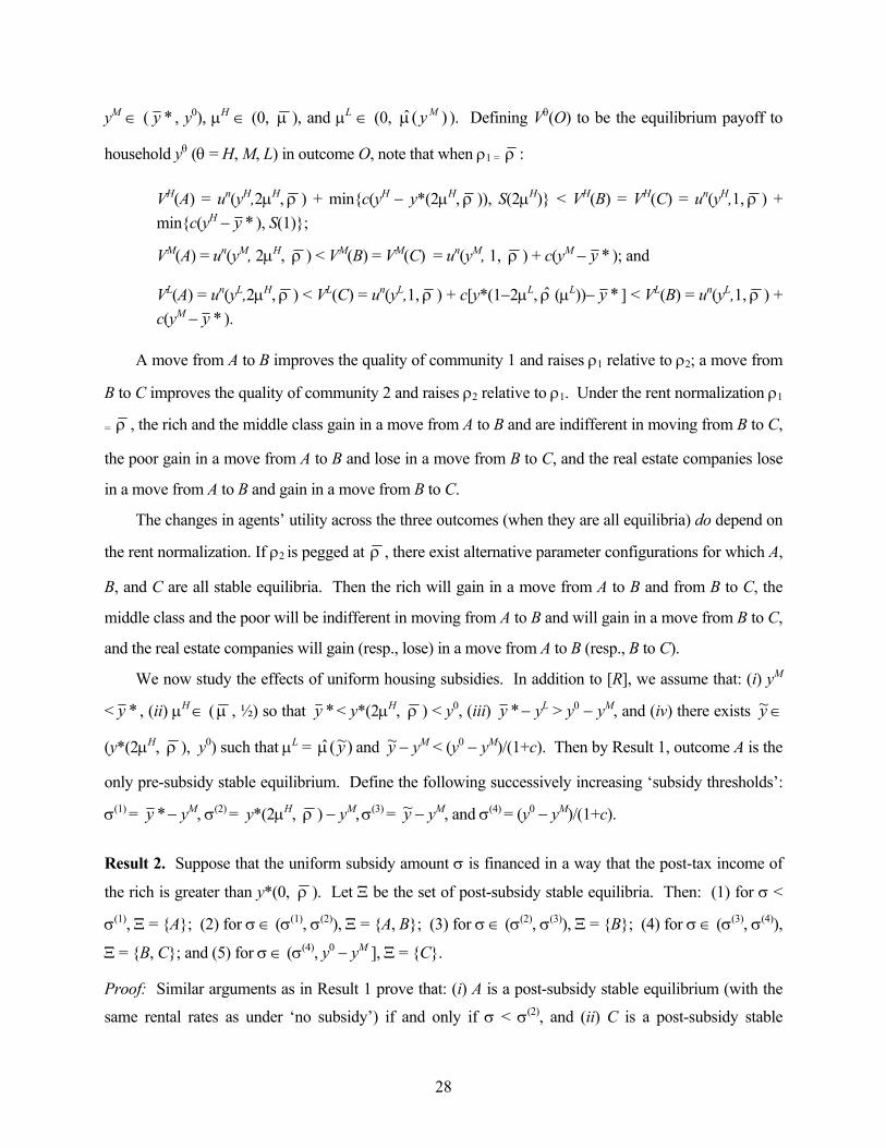
yM ∈ ( *y , y0), µH ∈ (0, µ ), and µL ∈ (0, ). Defining V)(ˆ Myµ θ(O) to be the equilibrium payoff to

household yθ (θ = H, M, L) in outcome O, note that when ρ1 = ρ :

ρ

VH(A) = un(yH,2µH, ρ ) + min{c(yH − y*(2µH, ρ )), S(2µH)} < VH(B) = VH(C) = un(yH,1, ρ ) + min{c(yH − *y ), S(1)};

VM(A) = un(yM, 2µH, ρ ) < VM(B) = VM(C) = un(yM, 1, ρ ) + c(yM − *y ); and

VL(A) = un(yL,2µH, ρ ) < VL(C) = un(yL,1, ) + c[y*(1−2µL, (µρ L))− *y ] < VL(B) = un(yL,1, ρ ) + c(yM − *y ).

A move from A to B improves the quality of community 1 and raises ρ1 relative to ρ2; a move from

B to C improves the quality of community 2 and raises ρ2 relative to ρ1. Under the rent normalization ρ1

= ρ , the rich and the middle class gain in a move from A to B and are indifferent in moving from B to C,

the poor gain in a move from A to B and lose in a move from B to C, and the real estate companies lose

in a move from A to B and gain in a move from B to C.

The changes in agents’ utility across the three outcomes (when they are all equilibria) do depend on

the rent normalization. If ρ2 is pegged at ρ , there exist alternative parameter configurations for which A,

B, and C are all stable equilibria. Then the rich will gain in a move from A to B and from B to C, the

middle class and the poor will be indifferent in moving from A to B and will gain in a move from B to C,

and the real estate companies will gain (resp., lose) in a move from A to B (resp., B to C).

We now study the effects of uniform housing subsidies. In addition to [R], we assume that: (i) yM

< *y , (ii) µH ∈ (µ , ½) so that *y < y*(2µH, ρ ) < y0, (iii) *y − yL > y0 − yM, and (iv) there exists ∈

(y*(2µ

y~

H, ρ ), y0) such that µL = and − y)~(ˆ yµ y~ M < (y0 − yM)/(1+c). Then by Result 1, outcome A is the

only pre-subsidy stable equilibrium. Define the following successively increasing ‘subsidy thresholds’:

σ(1) = *y − yM, σ(2) = y*(2µH, ρ ) − yM, σ(3) = − yy~ M, and σ(4) = (y0 − yM)/(1+c).

Result 2. Suppose that the uniform subsidy amount σ is financed in a way that the post-tax income of

the rich is greater than y*(0, ρ ). Let Ξ be the set of post-subsidy stable equilibria. Then: (1) for σ <

σ(1), Ξ = {A}; (2) for σ ∈ (σ(1), σ(2)), Ξ = {A, B}; (3) for σ ∈ (σ(2), σ(3)), Ξ = {B}; (4) for σ ∈ (σ(3), σ(4)),

Ξ = {B, C}; and (5) for σ ∈ (σ(4), y0 − yM ], Ξ = {C}.

Proof: Similar arguments as in Result 1 prove that: (i) A is a post-subsidy stable equilibrium (with the

same rental rates as under ‘no subsidy’) if and only if σ < σ(2), and (ii) C is a post-subsidy stable

28

equilibrium (with the same rental rates as under no subsidy), where all middle class households buy

homes with subsidy, if σ ∈ (σ(3), y0 − yM] and only if σ > σ(3). Now consider the post-subsidy outcome

B, where yM buys a home with subsidy in 1, and rents in 2. Then given ρ1 = ρ , indifference of yM

requires ρ2 = ρ2(B) − (1+c)σ (ρ2(B) as defined above). At these rents, yM strictly prefers to own in 1 if

and only if yM + σ > *y and strictly prefers to rent in 2 if and only if yM < y*(0, ρ2) = y0 − (1+c)σ. These

conditions are satisfied if and only if σ ∈ (σ(1), σ(4)). In B, ρ2 is lower post-subsidy than in the case of ‘no subsidies’ so as to make yM indifferent between renting in 2 and owning (with subsidy) in 1.

Thus, there are discrete improvements in the set of post-subsidy equilibria as σ crosses different

thresholds. Further, higher subsidies are needed to solve the coordination problem: when σ ∈ (σ(1),

σ(2)), while B is ‘attainable,’ the city may be stuck in A; this is solved by raising σ above σ(2).

Comparing household utility across the post-subsidy outcomes (for ρ1 = ρ ), all middle class and

poor households are strictly better off in B than in A; the middle class in community 1 gain from being

subsidy-financed homeowners, and those in community 2 gain from the post-subsidy rent decrease.

Then, if the ‘tax burden’ on the rich is not too large (i.e., a large part of the funds for subsidy can be

obtained by taxing the real estate companies), and if they care enough about civic quality (i.e., VHx(⋅) >>

VHy(⋅)), the rich are also better off in B. In contrast, no household is better off when the post-subsidy

outcome is C rather than B; while the middle class is indifferent, the rich are worse off because of the tax

burden, and the poor are worse off because of the increase in community 2 rent.

Next, we consider targeted subsidies where the middle class and the poor are given subsidies σM

and σL, respectively. Suppose that [R] holds, yM < *y , and µM ≤ µL. Then A is the only stable pre-

subsidy equilibrium. Consider the minimal subsidies needed to attain the ‘all owners {x1 = x2 = 1}’

outcome as the only post-subsidy equilibrium. It is easy to see that the middle class and the poor will be

better off under this outcome. The rich will also be better of provided the tax burden is not too large and

they care enough about civic quality. Define ≡ y*(1−2µ*y L, (µρ L)) and note that ∈ (*y *y , y0).

Result 3. Suppose that the post-tax income of the rich is always greater than y*(0, ρ ). Then, to attain

x1= x2=1 as the unique post-subsidy equilibrium, the least-cost uniform subsidy scheme (i.e., the one

with the smallest total subsidy bill) must set σ = max{y0 − yM, − y*y L}, while the least-cost targeted

subsidy scheme must set σM = y0 − yM and σL = − y*y L.

Proof: Let zM be the post-subsidy median income and zL the post-subsidy low income. If zM ≥ y0 and zL

29

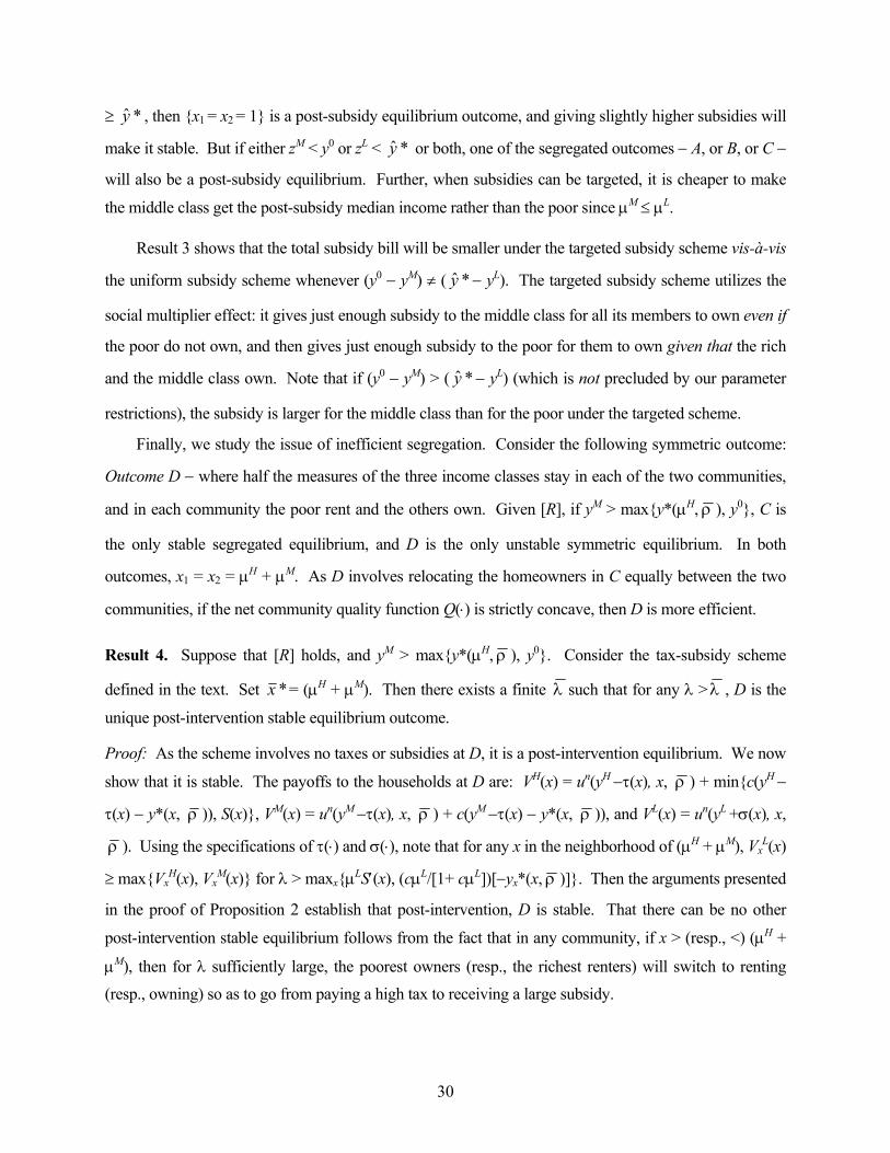
≥ , then {x*y 1 = x2 = 1} is a post-subsidy equilibrium outcome, and giving slightly higher subsidies will

make it stable. But if either zM < y0 or zL < or both, one of the segregated outcomes − A, or B, or C −

will also be a post-subsidy equilibrium. Further, when subsidies can be targeted, it is cheaper to make

the middle class get the post-subsidy median income rather than the poor since µ

*y

M ≤ µL.

Result 3 shows that the total subsidy bill will be smaller under the targeted subsidy scheme vis-à-vis

the uniform subsidy scheme whenever (y0 − yM) ≠ ( − y*y

*y

L). The targeted subsidy scheme utilizes the

social multiplier effect: it gives just enough subsidy to the middle class for all its members to own even if

the poor do not own, and then gives just enough subsidy to the poor for them to own given that the rich

and the middle class own. Note that if (y0 − yM) > ( − yL) (which is not precluded by our parameter

restrictions), the subsidy is larger for the middle class than for the poor under the targeted scheme.

Finally, we study the issue of inefficient segregation. Consider the following symmetric outcome:

Outcome D − where half the measures of the three income classes stay in each of the two communities,

and in each community the poor rent and the others own. Given [R], if yM > max{y*(µH, ρ ), y0}, C is

the only stable segregated equilibrium, and D is the only unstable symmetric equilibrium. In both

outcomes, x1 = x2 = µH + µM. As D involves relocating the homeowners in C equally between the two

communities, if the net community quality function Q(⋅) is strictly concave, then D is more efficient.

Result 4. Suppose that [R] holds, and yM > max{y*(µH, ρ ), y0}. Consider the tax-subsidy scheme

defined in the text. Set *x = (µH + µM). Then there exists a finite λ such that for any λ >λ , D is the

unique post-intervention stable equilibrium outcome.

Proof: As the scheme involves no taxes or subsidies at D, it is a post-intervention equilibrium. We now

show that it is stable. The payoffs to the households at D are: VH(x) = un(yH −τ(x), x, ρ ) + min{c(yH −

τ(x) − y*(x, ρ )), S(x)}, VM(x) = un(yM −τ(x), x, ρ ) + c(yM −τ(x) − y*(x, ρ )), and VL(x) = un(yL +σ(x), x,

ρ ). Using the specifications of τ(⋅) and σ(⋅), note that for any x in the neighborhood of (µH + µM), VxL(x)

≥ max{VxH(x), Vx

M(x)} for λ > maxx{µLS′(x), (cµL/[1+ cµL])[−yx*(x, ρ )]}. Then the arguments presented

in the proof of Proposition 2 establish that post-intervention, D is stable. That there can be no other

post-intervention stable equilibrium follows from the fact that in any community, if x > (resp., <) (µH +

µM), then for λ sufficiently large, the poorest owners (resp., the richest renters) will switch to renting (resp., owning) so as to go from paying a high tax to receiving a large subsidy.

30

References

Bénabou, Roland, “Workings of a City: Location, Education and Production,” Quarterly Journal of Economics, 1993, 103, 619-52.

——, “Equity and Efficiency in Human Capital Investment: The Local Connection,” Review of Economic Studies, 1996, 103, 619-52.

Besley, Timothy and Robin Burgess, “The Political Economy of Government Responsiveness: Theory and Evidence from India,” Quarterly Journal of Economics, 2002, 117, 1415-51.

Brock, William and Steven Durlauf, “Discrete Choice with Social Interactions,” Review of Economic Studies, 2001, 68, 235-60.

Buck, Andrew, Joseph Deutsch, Simon Hakim, Uriel Spiegel, and J. Weinblatt. “A Von Thünen Model of Crime, Casinos and Property Values in New Jersey,” Urban Studies, 1991, 28, 673-86.

Cohen, Cathy and Michael Dawson, “Neighborhood Poverty and African American Politics,” American Political Science Review, 1993, 87, 286-302.

Coulson, Edward, Seok-Joon Hwang, and Susumu Imai, “The Value of Owner-Occupation in Neighborhoods,” Pennsylvania State University, manuscript, 2001.

Cox, Kevin, “Housing Tenure and Neighborhood Activism,” Urban Affairs Quarterly, 1982, 18, 107-29.

Cutler, David, Edward Glaeser, and Jacob Vigdor, “The Rise and Decline of the American Ghetto,” Journal of Political Economy, 1999, 107, 455-506.

de Bartolome, Charles, “Equilibrium and Inefficiency in a Community Model with Peer Group Effects,” Journal of Political Economy, 1990, 98, 110-133.

Department of Housing and Urban Development, United States, The President's National Urban Policy Report, 1991, Washington DC.

DiPasquale, Denise and Edward Glaeser, “Incentives and Social Capital: Are Homeowners Better Citizens?” Journal of Urban Economics, 1999, 45, 354-84.

Durlauf, Steven, “Neighborhood Feedbacks, Endogenous Stratification, and Income Inequality,” in W. Barnett, G. Gandolfo, and C. Hillinger, eds., Proceedings of the Sixth International Symposium on Economic Theory and Econometrics, Cambridge: Cambridge University Press, 1996.

——, “Neighborhood Effects,” 2003, forthcoming in: Handbook of Regional and Urban Economics, vol. 4, J. V. Henderson and J.-F. Thisse, eds..

Fernandez, Raquel, “Sorting, Education and Inequality,” National Bureau of Economic Research, Working Paper no. 8101, 2001.

Fernandez, Raquel, and Richard Rogerson, “Income Distribution, Communities, and the Quality of Public Education,” Quarterly Journal of Economics, 1996, 111, 135-64.

Galor, Oded, and Joseph Zeira, “Income Distribution and Macroeconomics,” Review of Economic Studies, 1993, 60, 35-52.

Green, Richard, and Michelle White, “Measuring the Benefits of Home-owning on Children,” Journal of Urban Economics, 1997, 41, 441-61.

Helsley, Robert, and William Strange, “Social Interactions and the Institutions of Local Government,” American Economic Review, 2000, 90, 1477-90.

31

Henderson, J. Vernon and Yannis Ioannides, “A Model of Housing Tenure Choice,” American Economic Review, 1983, 73, 98-113.

Jargowsky, Paul, Poverty and Place: Ghettos, Barrios, and the American City, New York, Russell Sage Foundation, 1997.

Katz, Lawrence, Jeffrey Kling, and Jeffrey Liebman, “Moving to Opportunity in Boston: Early Results of a Randomized Mobility Experiment,” Quarterly Journal of Economics 2001, 116, 607-54.

Legros, Patrick, and Andrew Newman, “Wealth Effects, Distribution, and the Theory of Organization,” Journal of Economic Theory, 1996, 70, 312-41.

Leventhal, Tama and Jeanne Brooks-Gunn, “The Neighborhoods They Live in: The Effects of Neighborhood Residence on Child and Adolescent Outcomes,” Psychological Bulletin, 2000, 126, 309-37.

Massey, Douglas, and Nancy Denton, “The Dimensions of Residential Segregation,” Social Forces, 1988, 67, 281-315.

Merry, Sally Engle, Urban Danger: Life in a Neighborhood of Strangers. Philadelphia: Temple University Press, 1981.

Mookherjee, Dilip and Debraj Ray, “Contractual Structure and Wealth Accumulation,” American Economic Review, 2002, 92, 818-49.

Pargal, Sheoli, and David Wheeler, “Informal Regulation of Industrial Pollution in Developing Countries: Evidence from Indonesia,” Journal of Political Economy, 1996, 104, 1314-27.

Reynolds, A., The Appraisal of Real Estate, The Appraisal Institute, 8th Edition, 1983.

Rohe, William, and Michael Stegman, “The Impact of Homeownership on the Social and Political Involvement of Low-Income People,” Urban Affairs Quarterly, 1994, 30, 152-74.

Rosen, Harvey, “Housing Subsidies: Effect on Housing Decisions, Efficiency, and Equity,” in A. Auerbach and M. Feldstein, eds., Handbook of Public Economics, vol. I, Amsterdam: North-Holland, 1985.

Savage, Howard, “Who Could Afford to Buy a House in 1995?” US Department of Commerce, Census Bureau, 1999. http://www.census/gov/hhes/www/hsgaffrd.html.

Schelling, Thomas, “Dynamic Models of Segregation,” Journal of Mathematical Sociology, 1971, 1,2, 143-186.

Simon, William, “Social-Republican Property,” UCLA Law Review, 1991, 38, 1335-1413.

Smith, V. Kerry and Ju-Chin Huang, “Can Markets Value Air Quality? A Meta-analysis of Hedonic Property Value Models, Journal of Political Economy, 1995, 103, 209-27.

Stromberg, David, “Radio’s Impact on Public Spending,” Quarterly Journal of Economics, 2004, 119, 189-221.

Verba, Sidney, Kay Lehman Schlozman, and Henry Brady, Voice and Equality: Civic Voluntarism in American Politics. Cambridge, MA: Harvard University Press, 1995.

32

Table 1. Local civic participation in the US: Homeowners compared to renters

Source Dimensions of civic participation Effect of homeownership

Control variables

Cox 1982: Survey of 500 residents of Columbus, Ohio

Probability of neighborhood activism • when facing a community problem • in other cases

0.39** 0.27**

Number of children in household

Rohe and Stegman 1994: Longitudinal study of 226 low-income homebuyers and renters in Baltimore

Number of community organizations that a resident household belongs to

0.20**

Income, education, age, race, gender, marital status, children, dwelling type, satisfaction with neighborhood

Verba et al. 1995: Citizenship Participation Study of a cross-section of 15,000 adults in the US

Probability of local participation, e.g., voting in local elections, contacting local officials, protesting on local issues, attending local board meetings

0.09**

Years in the community, income, education, race, gender, job level, parents’ education, free time, school-aged children

OLS IV Probability of voting in local elections 0.15** 0.28*

Number of non-professional organi-zations that a household belongs to

0.25** 0.59**

DiPasquale and Glaeser 1999: US General Social Survey

Probability of knowing the identity of the school board head

0.09** 0.46**

Income, education, age, race, gender, marital status, children, city size

**significant at 1% level; *significant at 5% level.

Table 2. Dissimilarity index of homeowner-renter segregation in the ten largest US MSAs, 1990

Annual income Non-blacks with children

Non-blacks, no children

Blacks with children

Blacks, no children

< $25,000 0.624 0.450 0.676 0.619

$25,000−50,000 0.423 0.351 0.576 0.618

$50,000−75,000 0.424 0.354 0.600 0.669

$75,000−100,000 0.570 0.414 0.799 0.824

> $100,000 0.610 0.438 0.878 0.871

Data Source: 1990 US Census

33

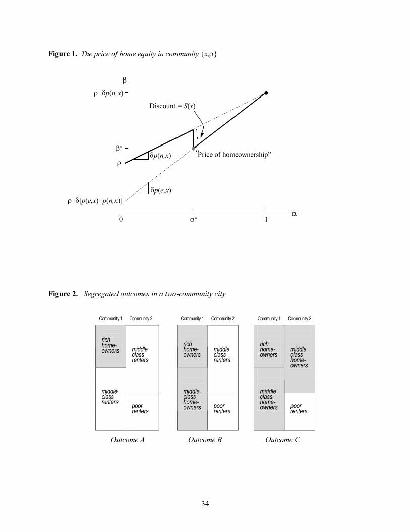
Figure 1. The price of home equity in community {x,ρ}

0 1 α ∗ α

β

β ∗

Discount = S(x)

δ p (n,x)

δ p (e,x)

“ Price of homeownership”

ρ – δ [ p (e,x) – p (n,x)]

ρ

ρ + δ p (n,x)

Figure 2. Segregated outcomes in a two-community city

Community 1 Community 2 Community 1 Community 2 Community 1 Community 2 rich home-owners

rich home-owners

rich home-owners

middle class renters

middle class renters

middle class home-owners

middle class renters

poor renters

middle class home-owners

poor renters

middle class home-owners

poor renters

Outcome A Outcome B Outcome C

34