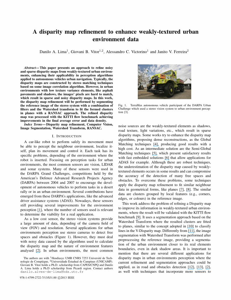
A disparity map refinement to enhance weakly-textured urban

environment data

Danilo A. Lima1, Giovani B. Vitor1,2, Alessandro C. Victorino1 and Janito V. Ferreira2

Abstract— This paper presents an approach to refine noisyand sparse disparity maps from weakly-textured urban environ-ments, enhancing their applicability in perception algorithmsapplied to autonomous vehicles urban navigation. Typically, thedisparity maps are constructed by stereo matching techniquesbased on some image correlation algorithm. However, in urbanenvironments with low texture variance elements, like asphaltpavements and shadows, the images’ pixels are hard to match,which result in sparse and noisy disparity maps. In this work,the disparity map refinement will be performed by segmentingthe reference image of the stereo system with a combination offilters and the Watershed transform to fit the formed clustersin planes with a RANSAC approach. The refined disparitymap was processed with the KITTI flow benchmark achievingimprovements in the final average error and data density.

Index Terms— Disparity map refinement, Computer Vision,Image Segmentation, Watershed Transform, RANSAC.

I. INTRODUCTION

A car-like robot to perform safely its movement must

be able to percept the neighbour environment, localize it-

self, plan its movement and control it. Each task has its

specific problems, depending of the environment where the

robot is inserted. Focusing on perception tasks for urban

environments, the most common sensors are vision, LIDAR

and sonar systems. Many of these sensors were used in

the DARPA Grand Challenges, competitions held by the

American’s Defence Advanced Research Projects Agency

(DARPA) between 2004 and 2007 to encourage the devel-

opment of autonomous vehicles to perform tasks in a desert

rally or in an urban environment. Several contributions have

emerged from these DARPA’s applications, like the advanced

driver assistance systems (ADAS). Nowadays, these sensors

still providing several improvements for the environment

perception [1], where the number of sensors used is relevant

to determine the viability for a real application.

As a low cost sensor, the stereo vision systems provide

a large amount of data, depending of the camera field of

view (FOV) and resolution. Several applications for urban

environments perception use stereo cameras to detect free

spaces and obstacles (Figure 1). However, they must deal

with noisy data caused by the algorithms used to calculate

the disparity map and the nature of environment features

analysed [2]. In urban environments, the most common

The authors are with 1Heudiasyc UMR CNRS 7253 Universite de Tech-nologie de Compiegne, 2Universidade Estadual de Campinas (UNICAMP).Giovani B. Vitor holds a Ph.D. scholarship from CAPES/CNPQ and DaniloA. Lima holds a Ph.D scholarship from Picardi region. Contact authorsdanilo.alves-de-lima@hds.utc.fr

Fig. 1. TerraMax autonomous vehicle participant of the DARPA UrbanChallenge which used a stereo vision system to urban environment percep-tion [3].

noise sources are the weakly-textured elements as shadows,

road texture, light variations, etc., which result in sparse

disparity maps. Some works try to enhance the disparity map

algorithms, proposing dense reconstructions, as the Global

Matching techniques [4], producing good results with a

high cost. As an intermediate solution are the Semi-Global

Matching techniques [5], which present satisfactory results

with fast embedded solutions [6] that allow applications for

ADAS for example. Although these are robust techniques,

the underestimation of the disparity map caused by weakly-

textured elements occurs in some results and can compromise

the accuracy of the detection of many free spaces and

obstacles. To overcome these problems, some techniques

apply the disparity map refinement to fit similar neighbour

data in geometrical forms, like planes [7], [8]. The similar

data are clusters grouped by local features (e.g., corners,

edges, or colours) in the reference image.

This work address the problem of refining a Disparity map

to improve its information in weakly-textured urban environ-

ments, where the result will be validated with the KITTI flow

benchmark [9]. It uses a segmentation approach based on the

Watershed Transform where the resulted clusters are fitted

to planes, similar to the concept adopted in [10] to classify

lines in the V-Disparity map. Differently from [11], the image

segmentation with Watershed Transform was performed after

preprocessing the reference image, providing a segmenta-

tion of the urban environment closer to its real elements

boundaries, even in dark shadow areas. It is important to

mention that there are several different applications for

disparity maps in urban environments perception where the

current refinement and segmentation approaches could be

applied, as in road and obstacles detection [12], [13], [2],

as well with techniques that incorporate more sensors to

978-1-4799-2722-7/13/$31.00 c©2013 IEEE

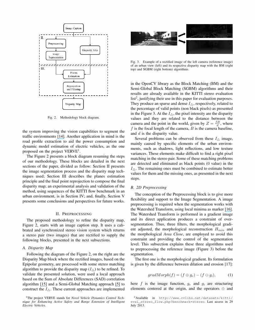
Fig. 2. Methodology block diagram.

the system improving the vision capabilities to segment the

traffic environments [14]. Another application in mind is the

road profile extraction to aid the power consumption and

dynamic model estimation of electric vehicles, as the one

proposed on the project VERVE1.

The Figure 2 presents a block diagram resuming the steps

of our methodology. These blocks are detailed in the next

sections of the paper, divided as follow: Section II presents

the image segmentation process and the disparity map tech-

niques used; Section III describes the planes estimation

principle and the final point reprojection to compose the final

disparity map; an experimental analysis and validation of the

method, using sequences of the KITTI flow benchmark in an

urban environment, is in Section IV; and, finally, Section V

presents some conclusions and perspectives for future works.

II. PREPROCESSING

The proposed methodology to refine the disparity map,

Figure 2, starts with an image caption step. It uses a cali-

brated and synchronized stereo vision system which returns

a stereo pair (two images) that are rectified to supply the

following blocks, presented in the next subsections.

A. Disparity Map

Following the diagram of the Figure 2, on the right are the

Disparity Map block where the rectified images, based on the

Epipolar geometry, are processed with some stereo matching

algorithm to provide the disparity map (I△) to be refined. To

validate the presented solution, were used a local approach

based on the Sum of Absolute Differences (SAD) correlation

algorithm [15] and a Semi-Global Matching approach [5] to

construct the I△. These current approaches are implemented

1The project VERVE stands for Novel Vehicle Dynamics Control Tech-

nique for Enhancing Active Safety and Range Extension of Intelligent

Electric Vehicles.

Fig. 3. Example of a rectified image of the left camera (reference image)of an urban view (left) and its respective disparity map with the BM (righttop) and SGBM (right bottom) algorithms.

in the OpenCV library as the Block Matching (BM) and the

Semi-Global Block Matching (SGBM) algorithms and their

results are already available in the KITTI stereo evaluation

list2, justifying their use in this paper for evaluation purposes.

They produce an sparse and dense I△, respectively, related to

the percentage of valid points (non black pixels) as presented

in the Figure 3. At the I△, the pixel intensity are the disparity

values and they are related to the distance between the

camera and the point in the world, given by Z = fBd

, where

f is the focal length of the camera, B is the camera baseline,

and d is the disparity value.

Several problems can be observed from these I△ image,

mainly caused by specific elements of the urban environ-

ments, such as shadows, light reflections, and low texture

variances. These elements make difficult to find a right pixel

matching in the stereo pair. Some of these matching problems

are detected and eliminated as black points (0 value) in the

I△. The remaining ones must be combined to estimate better

values for them and the missing ones, as presented in the next

steps.

B. 2D Preprocessing

The conception of the Preprocessing block is to give more

flexibility and support to the Image Segmentation. A image

preprocessing is required when the segmentation works with

the Watershed Transform, using local minima as marker [16].

The Watershed Transform is performed in a gradient image

and its direct application produces a constraint of over-

segmentation. Thus, three filters, the morphological gradi-

ent adjusted, the morphological reconstruction Hmin and

the morphological Area Close, are employed to avoid this

constraint and providing the control of the segmentation

level. This subsection explains these three algorithms used

to preprocessing the reference image (Figure 3) before the

segmentation.

The first one is the morphological gradient. Its formulation

is given by the difference between dilation and erosion [17]:

gradMorph(f) = (f ⊕ ge)− (f ⊖ gi), (1)

here f is the image function, ge and gi are structuring

elements centered at the origin, and the operators ⊕ and

2Available in http://www.cvlibs.net/datasets/kitti/

eval_stereo_flow.php?benchmark=stereo. Last access in 29July 2013.

(a)

(b)

(c)

Fig. 4. Enhancing the contrast of higher frequency in shadow areas. (a)Original image, (b) gradient image and (c) the gradient image with shadowarea enhanced.

⊖ are respectively dilation and erosion (see [17] for more

details).

In the early work [2], was observed that the low-contrast

of higher frequency in shadow areas of the image provides

a not correct segmentation by merging different regions. To

avoid this drawback, it is proposed an enhancement on the

areas where the shadow occur. It is performed applying a

threshold in the grayscale original image to detect the shadow

areas, where the grayscale value was set to 50 (to detect dark

regions), and after is calculated a non-linear transform at the

value of the gradient image increasing the contrast in this

detected area. This transformation is given by the equation 2,

which x represents the gradient intensity, c the constant of

normalization and γ another constant factor setted to 0.45.

These process is showed in the Figure 4.

f(x) = cxγ . (2)

After extracting higher frequencies from the reference

image by the morphological gradient filter, the next step

consists in using the Area Close to filter out pixels where

their connected component area is smaller than a given

parameter λ. Here is provided the definitions of Area Open

once Area Close is its complement [18]. The connected

component is defined as a pixels set characterized by a

relation between their neighbourhood on the binary image

M ⊂ IR2. First, the connected opening Cx(X) of a set

X ⊆ M at point x ∈ X is the connected component of

X containing x if x ∈ X and 0 otherwise. The binary area

opening is then defined on subsets of M [19].

γaλ(X) = {x ∈ X | Area(Cx(X)) ≥ λ}. (3)

The γaλ(X) denote the morphological area opening with

respect to the structure element a and the parameter λ. The

Area(.) is the number of elements in a connected component

of Cx(X). Its dual binary area closing is obtained as:

φaλ(X) = [γa

λ(Xc)]c, (4)

where Xc denotes the complement of X in M . Extending

the filter for a mapping f : M → IR, in a grayscale image,

then the area opening γaλ(f) is given by:

(γaλ(f))(x) = sup{h ≤ f(x) | x ∈ γa

λ(Th(f))}. (5)

In the Equation 5, Th(f) represents the threshold of f at

value h:

Th(f) = {x ∈ M | f(x) ≥ h}. (6)

As mentioned before, the complement of equation 5 can

be similarly extended to the conception of area closing to

mappings from M → IR.

Finally, the last algorithm applied has the function of

filter out the regional minima. It uses the morphological

reconstruction Hmin, obtained by successive geodesics dila-

tions. This principle employs two subsets of IR2, called mask

image and marker image, with the same size. Moreover, the

maskimage must have intensity values higher than or equal

to those from marker image [19]. Properly performing the

reconstruction H-maxima or Hmax, is possible to take the

H-minima or Hmin from its complement. Mathematically,

defining mask image as I and marker image as I −h, being

h the parameter to filter, the equation is given by [17]:

Hmaxah(I) = I∆a(I − h). (7)

In this definition, ∆ stands for morphological reconstruc-

tion with the structure element a. By duality, the Hmin is

defined as:

Hminah(I) = [Ic∆a(I

c − h)]c. (8)

Studying different approaches, the Watershed Transform

has different definitions at the literature, each one producing

a different solution set, presented in [20]. The definitions

are based on regional or global elements, such as influence

zones and shortest-path forests with maximum or sum of

weights of edges, or on local elements, such as the steepest

descent paths. In this work, the local condition definition

was used, called LC-WT (Local Condition Watershed Trans-

form), which is defined as the steepest descent paths, where

the neighbours information is used to create a path to the

corresponding minimum. More details are found in [16].

The principle of this disparity map refinement is to asso-

ciate the weakly-textured elements, like asphalt pavements

and shadows, to segmented regions in the reference image,

fitting a plane to each one of them, as well as, reduce the

pixel variation in all regions. As mentioned, there are several

works that use this analogy. In fact, what distinguishes this

work is the way the image is segmented. The combination

of these three filters with the Watershed Transform provides

a different methodology to determine the resulted segmenta-

tion.

To demonstrate the processing done by this two blocks,

the output of the segmentation can be seen in the Figure 5.

Notice that the main point of this approach is choose the

value of the parameters λ and h of the Preprocessing Block.

In fact, these parameters give an excellent flexibility to de-

termine the segmentation result of the Watershed Transform

which is responsible to generate the representatives samples

associated with the Disparity map.

III. REMAPPING

A. Planes Estimation

Based on the assumption that pixels in a segment are co-

planar, plane estimation is one of the most efficient ways for

disparity refinement [8]. Similarly thought by [10] which

found the navigable area by approximating small planes

in the world by lines in the V-Disparity map, this work

uses the RANSAC method to estimate plane coefficients on

segments defined on the reference image with the points of

the disparity map.

RANSAC based plane estimation is a minimization algo-

rithm that can exclude the outliers where three points are

randomly chosen to calculate the plane function during each

iteration. Its accuracy is estimated by counting the number

of points within the segment that agree with the given plane,

like consensus. In this way, the plane fitting is performed

with the points of the Disparity Map being P = (x, y, d)and Cp(s) being the set of segment points s. To each Cp(s),the plane function estimated is given by the equation (9):

n · (P − P0) = 0, (9)

where n is the nonzero vector normal to the plane, P0 is a

know point in the plane, P is a given point to determine if

it is in the plane, and (·) means a dot product.

B. Disparity Map Reprojection and Filtering

For each cluster’s fitted plane, the Disparity image (I△)

can be reprojected applying its points in the respective plane

equation. However, due to the nature of the RANSAC and

the nonlinear variation of the disparity data, the final plane is

only a estimation that can be good or not, depending of the

points used in the process. Therefore, the I△’s points must

respect the follow statements to be fit:

• The pixel disparity value is in a interval where a small

variation in its value does not represents a large change

in the Z distance, in the world (e.g., variation bigger

than 2 meters, based in the relation presented in II-A);

• The segment have enough percentage of valid points

(disparity value different of zero);

• The maximum number of interactions to fit the plane

was not reached;

• The point reprojected do not highly diverge from its

original value (which is different from zero).

The highly divergence mentioned in the last statement is

determined by the difference between the disparity value

in I△ and the reprojected disparity value. Following these

statements the Refined Disparity map I△r is acquired.

IV. EXPERIMENTAL RESULTS

In this section is presented the results for the Disparity

map refinement, demonstrating the influence of the param-

eters λ and H on the image segmentation resulted, as

well as its validation in the final result of the proposed

method. The methodology was tested with the KITTI flow

benchmark [9] acquired under a static environment, including

194 training and 195 test image pairs of diversified urban

(a)

(b)

(c)

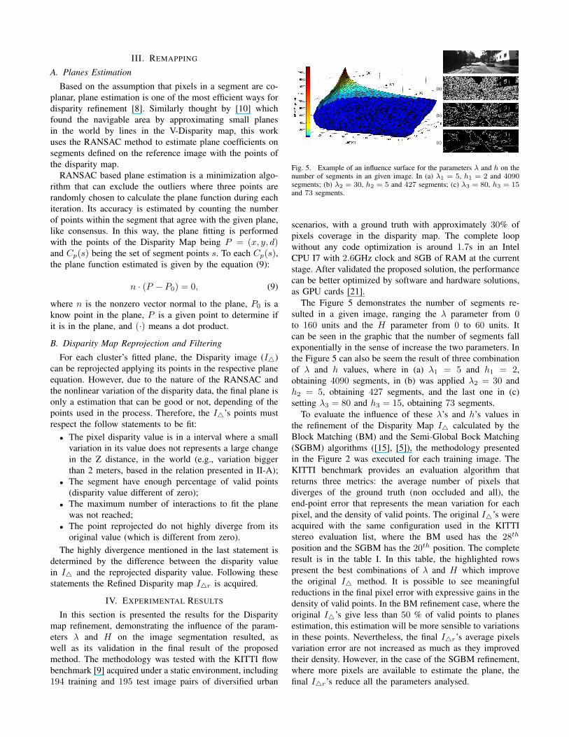
Fig. 5. Example of an influence surface for the parameters λ and h on thenumber of segments in an given image. In (a) λ1 = 5, h1 = 2 and 4090

segments; (b) λ2 = 30, h2 = 5 and 427 segments; (c) λ3 = 80, h3 = 15

and 73 segments.

scenarios, with a ground truth with approximately 30% of

pixels coverage in the disparity map. The complete loop

without any code optimization is around 1.7s in an Intel

CPU I7 with 2.6GHz clock and 8GB of RAM at the current

stage. After validated the proposed solution, the performance

can be better optimized by software and hardware solutions,

as GPU cards [21].

The Figure 5 demonstrates the number of segments re-

sulted in a given image, ranging the λ parameter from 0to 160 units and the H parameter from 0 to 60 units. It

can be seen in the graphic that the number of segments fall

exponentially in the sense of increase the two parameters. In

the Figure 5 can also be seem the result of three combination

of λ and h values, where in (a) λ1 = 5 and h1 = 2,

obtaining 4090 segments, in (b) was applied λ2 = 30 and

h2 = 5, obtaining 427 segments, and the last one in (c)

setting λ3 = 80 and h3 = 15, obtaining 73 segments.

To evaluate the influence of these λ’s and h’s values in

the refinement of the Disparity Map I△ calculated by the

Block Matching (BM) and the Semi-Global Bock Matching

(SGBM) algorithms ([15], [5]), the methodology presented

in the Figure 2 was executed for each training image. The

KITTI benchmark provides an evaluation algorithm that

returns three metrics: the average number of pixels that

diverges of the ground truth (non occluded and all), the

end-point error that represents the mean variation for each

pixel, and the density of valid points. The original I△’s were

acquired with the same configuration used in the KITTI

stereo evaluation list, where the BM used has the 28th

position and the SGBM has the 20th position. The complete

result is in the table I. In this table, the highlighted rows

present the best combinations of λ and H which improve

the original I△ method. It is possible to see meaningful

reductions in the final pixel error with expressive gains in the

density of valid points. In the BM refinement case, where the

original I△’s give less than 50 % of valid points to planes

estimation, this estimation will be more sensible to variations

in these points. Nevertheless, the final I△r’s average pixels

variation error are not increased as much as they improved

their density. However, in the case of the SGBM refinement,

where more pixels are available to estimate the plane, the

final I△r’s reduce all the parameters analysed.

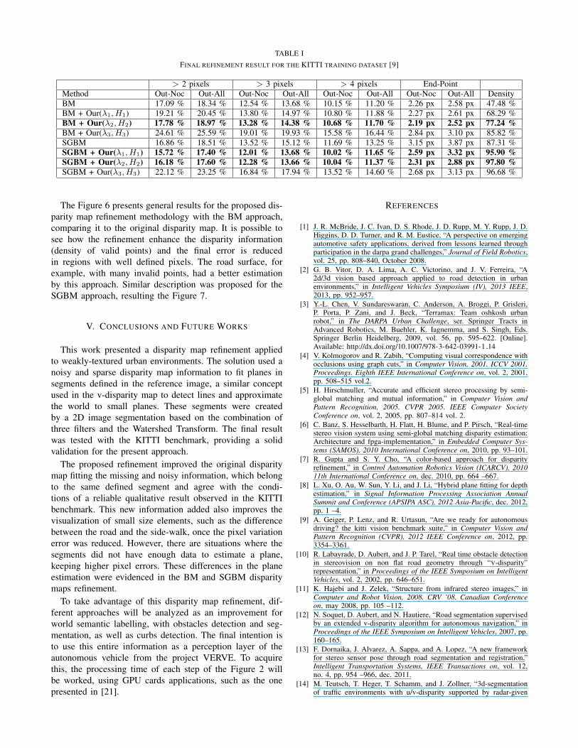
TABLE I

FINAL REFINEMENT RESULT FOR THE KITTI TRAINING DATASET [9]

> 2 pixels > 3 pixels > 4 pixels End-PointMethod Out-Noc Out-All Out-Noc Out-All Out-Noc Out-All Out-Noc Out-All DensityBM 17.09 % 18.34 % 12.54 % 13.68 % 10.15 % 11.20 % 2.26 px 2.58 px 47.48 %BM + Our(λ1, H1) 19.21 % 20.45 % 13.80 % 14.97 % 10.80 % 11.88 % 2.27 px 2.61 px 68.29 %BM + Our(λ2, H2) 17.78 % 18.97 % 13.28 % 14.38 % 10.68 % 11.70 % 2.19 px 2.52 px 77.24 %

BM + Our(λ3, H3) 24.61 % 25.59 % 19.01 % 19.93 % 15.58 % 16.44 % 2.84 px 3.10 px 85.82 %SGBM 16.86 % 18.51 % 13.52 % 15.12 % 11.69 % 13.25 % 3.15 px 3.87 px 87.31 %SGBM + Our(λ1, H1) 15.72 % 17.40 % 12.01 % 13.68 % 10.02 % 11.65 % 2.59 px 3.32 px 95.90 %

SGBM + Our(λ2, H2) 16.18 % 17.60 % 12.28 % 13.66 % 10.04 % 11.37 % 2.31 px 2.88 px 97.80 %

SGBM + Our(λ3, H3) 22.12 % 23.25 % 16.84 % 17.94 % 13.52 % 14.60 % 2.68 px 3.13 px 96.68 %

The Figure 6 presents general results for the proposed dis-

parity map refinement methodology with the BM approach,

comparing it to the original disparity map. It is possible to

see how the refinement enhance the disparity information

(density of valid points) and the final error is reduced

in regions with well defined pixels. The road surface, for

example, with many invalid points, had a better estimation

by this approach. Similar description was proposed for the

SGBM approach, resulting the Figure 7.

V. CONCLUSIONS AND FUTURE WORKS

This work presented a disparity map refinement applied

to weakly-textured urban environments. The solution used a

noisy and sparse disparity map information to fit planes in

segments defined in the reference image, a similar concept

used in the v-disparity map to detect lines and approximate

the world to small planes. These segments were created

by a 2D image segmentation based on the combination of

three filters and the Watershed Transform. The final result

was tested with the KITTI benchmark, providing a solid

validation for the present approach.

The proposed refinement improved the original disparity

map fitting the missing and noisy information, which belong

to the same defined segment and agree with the condi-

tions of a reliable qualitative result observed in the KITTI

benchmark. This new information added also improves the

visualization of small size elements, such as the difference

between the road and the side-walk, once the pixel variation

error was reduced. However, there are situations where the

segments did not have enough data to estimate a plane,

keeping higher pixel errors. These differences in the plane

estimation were evidenced in the BM and SGBM disparity

maps refinement.

To take advantage of this disparity map refinement, dif-

ferent approaches will be analyzed as an improvement for

world semantic labelling, with obstacles detection and seg-

mentation, as well as curbs detection. The final intention is

to use this entire information as a perception layer of the

autonomous vehicle from the project VERVE. To acquire

this, the processing time of each step of the Figure 2 will

be worked, using GPU cards applications, such as the one

presented in [21].

REFERENCES

[1] J. R. McBride, J. C. Ivan, D. S. Rhode, J. D. Rupp, M. Y. Rupp, J. D.Higgins, D. D. Turner, and R. M. Eustice, “A perspective on emergingautomotive safety applications, derived from lessons learned throughparticipation in the darpa grand challenges,” Journal of Field Robotics,vol. 25, pp. 808–840, October 2008.

[2] G. B. Vitor, D. A. Lima, A. C. Victorino, and J. V. Ferreira, “A2d/3d vision based approach applied to road detection in urbanenvironments,” in Intelligent Vehicles Symposium (IV), 2013 IEEE,2013, pp. 952–957.

[3] Y.-L. Chen, V. Sundareswaran, C. Anderson, A. Broggi, P. Grisleri,P. Porta, P. Zani, and J. Beck, “Terramax: Team oshkosh urbanrobot,” in The DARPA Urban Challenge, ser. Springer Tracts inAdvanced Robotics, M. Buehler, K. Iagnemma, and S. Singh, Eds.Springer Berlin Heidelberg, 2009, vol. 56, pp. 595–622. [Online].Available: http://dx.doi.org/10.1007/978-3-642-03991-1 14

[4] V. Kolmogorov and R. Zabih, “Computing visual correspondence withocclusions using graph cuts,” in Computer Vision, 2001. ICCV 2001.

Proceedings. Eighth IEEE International Conference on, vol. 2, 2001,pp. 508–515 vol.2.

[5] H. Hirschmuller, “Accurate and efficient stereo processing by semi-global matching and mutual information,” in Computer Vision and

Pattern Recognition, 2005. CVPR 2005. IEEE Computer Society

Conference on, vol. 2, 2005, pp. 807–814 vol. 2.

[6] C. Banz, S. Hesselbarth, H. Flatt, H. Blume, and P. Pirsch, “Real-timestereo vision system using semi-global matching disparity estimation:Architecture and fpga-implementation,” in Embedded Computer Sys-

tems (SAMOS), 2010 International Conference on, 2010, pp. 93–101.

[7] R. Gupta and S. Y. Cho, “A color-based approach for disparityrefinement,” in Control Automation Robotics Vision (ICARCV), 2010

11th International Conference on, dec. 2010, pp. 664 –667.

[8] L. Xu, O. Au, W. Sun, Y. Li, and J. Li, “Hybrid plane fitting for depthestimation,” in Signal Information Processing Association Annual

Summit and Conference (APSIPA ASC), 2012 Asia-Pacific, dec. 2012,pp. 1 –4.

[9] A. Geiger, P. Lenz, and R. Urtasun, “Are we ready for autonomousdriving? the kitti vision benchmark suite,” in Computer Vision and

Pattern Recognition (CVPR), 2012 IEEE Conference on, 2012, pp.3354–3361.

[10] R. Labayrade, D. Aubert, and J. P. Tarel, “Real time obstacle detectionin stereovision on non flat road geometry through “V-disparity”representation,” in Proceedings of the IEEE Symposium on Intelligent

Vehicles, vol. 2, 2002, pp. 646–651.

[11] K. Hajebi and J. Zelek, “Structure from infrared stereo images,” inComputer and Robot Vision, 2008. CRV ’08. Canadian Conference

on, may 2008, pp. 105 –112.

[12] N. Soquet, D. Aubert, and N. Hautiere, “Road segmentation supervisedby an extended v-disparity algorithm for autonomous navigation,” inProceedings of the IEEE Symposium on Intelligent Vehicles, 2007, pp.160–165.

[13] F. Dornaika, J. Alvarez, A. Sappa, and A. Lopez, “A new frameworkfor stereo sensor pose through road segmentation and registration,”Intelligent Transportation Systems, IEEE Transactions on, vol. 12,no. 4, pp. 954 –966, dec. 2011.

[14] M. Teutsch, T. Heger, T. Schamm, and J. Zollner, “3d-segmentationof traffic environments with u/v-disparity supported by radar-given

Fig. 6. Result for the Disparity map refinement of the BM method in different urban conditions.

Fig. 7. Result for the Disparity map refinement of the SGBM method in different urban conditions.

masterpoints,” in Intelligent Vehicles Symposium (IV), 2010 IEEE, june2010, pp. 787 –792.

[15] T. K. Hiroshi, H. Kano, S. Kimura, A. Yoshida, and K. Oda, “Develop-ment of a video-rate stereo machine,” in IROS ’95: Proceedings of the

International Conference on Intelligent Robots and Systems-Volume 3.Washington, DC, USA: IEEE Computer Society, 1995, p. 3095.

[16] R. Audigier and R. de Alencar Lotufo, “Relationships between somewatershed definitions and their tie-zone transforms,” Image Vision

Comput., vol. 28, no. 10, pp. 1472–1482, Oct. 2010. [Online].Available: http://dx.doi.org/10.1016/j.imavis.2009.11.002

[17] E. R. Dougherty and R. A. Lotufo, Hands-on Morphological Image

Processing (SPIE Tutorial Texts in Optical Engineering Vol. TT59).SPIE Publications, Jul. 2003.

[18] A. Meijster and M. H. F. Wilkinson, “A comparison of algorithms for

connected set openings and closings,” Pattern Analysis and Machine

Intelligence, IEEE Transactions on, vol. 24, no. 4, pp. 484–494, 2002.

[19] L. Vincent, “Morphological grayscale reconstruction in image anal-ysis: applications and efficient algorithms,” Image Processing, IEEE

Transactions on, vol. 2, no. 2, pp. 176–201, Apr.

[20] J. B. T. M. Roerdink and A. Meijster, “The watershed transform:Definitions, algorithms and parallelization strategies,” 2001.

[21] A. Korbes, G. Vitor, R. de Alencar Lotufo, and J. Ferreira, “Ad-vances on watershed processing on gpu architecture,” in Mathematical

Morphology and Its Applications to Image and Signal Processing,ser. Lecture Notes in Computer Science, P. Soille, M. Pesaresi, andG. Ouzounis, Eds. Springer Berlin / Heidelberg, 2011, vol. 6671, pp.260–271.