Efficient Sampling of Disparity Spacefor Fast And Accurate Matching

Jan Cech and Radim SaraCenter for Machine Perception

Czech Technical University, Prague, Czech Republic{cechj,sara}@cmp.felk.cvut.cz

Abstract

A simple stereo matching algorithm is proposed that vis-its only a small fraction of disparity space in order to finda semi-dense disparity map. It works by growing from asmall set of correspondence seeds. Unlike in known seed-growing algorithms, it guarantees matching accuracy andcorrectness, even in the presence of repetitive patterns. Thissuccess is based on the fact it solves a global optimizationtask. The algorithm can recover from wrong initial seeds tothe extent they can even be random. The quality of corre-spondence seeds influences computing time, not the qualityof the final disparity map. We show that the proposed al-gorithm achieves similar results as an exhaustive disparityspace search but it is two orders of magnitude faster. This isvery unlike the existing growing algorithms which are fastbut erroneous. Accurate matching on 2-megapixel imagesof complex scenes is routinely obtained in a few seconds ona common PC from a small number of seeds, without limit-ing the disparity search range.

1. IntroductionTraditional area-based dense stereoscopic matching algo-rithms perform exhaustive search of the entire disparityspace, i.e. they need to compute a correlation statistic forall putative correspondences [18]. Although efficient im-plementations for computing most of the commonly usedstatistics (SSD, SAD, NCC) are known [20], this is still oneof the most expensive phases of stereo matching.

To avoid visiting the entire disparity space, algorithmswere proposed that greedily grow corresponding patchesfrom a given set of reliable seed correspondences. Suchalgorithms assume that neighboring pixels have similar dis-parity, not exceeding disparity gradient limit [15] or a simi-lar constraint.

The principle of growing a solution from initial seedshad long been known in segmentation [6]. The first algo-

rithms using this principle in stereo were proposed in pho-togrammetric community: by Otto and Chau [14], O’Neilland Denos [13], and by Kim and Muller [7].

Later, Lhuillier and Quan [9] employed the uniquenessconstraint and proposed an algorithm both with and withoutthe epipolar constraint in which images play a symmetricrole. This work has later been used in a 3D surface recon-struction pipeline [10]. The basic idea is to grow contiguouscomponents1 in disparity space from initial correspondenceseeds sorted in decreasing value of image similarity andto stop the growth process at image pixels where unique-ness constraint would be violated. The growth occurs in theneighborhood of previous matches in disparity space. Thiscreates new seeds that are put to the priority queue. A de-cision on match acceptance is never revised. This inherentgreediness of the algorithm may cause a complete failurein the presence of repetitive texture in the scene, as will bediscussed later.

Independently, Chen and Medioni [2] proposed an alter-native scheme in which the growth is not constrained byuniqueness. The best-first strategy is not used and the seedsare taken in arbitrary order. When a match of better imagesimilarity is found at a given pixel, it overrides the previ-ous match but it does not grow further, hence the correctionis only local and there is no ability to follow a new dis-parity component of high image similarity. If the seeds inthe queue are processed in a different order, (very) differ-ent results are obtained. Moreover, images in this algorithmdo not have a symmetric role, which means the resultingmatching violates uniqueness constraint.

The disadvantage of both approaches is that the decisionon a match is local in the sense that other matches do notinfluence it (no global optimization is involved).

The following two works use variations of the abovemethods which means they suffer from the same drawbacks,especially in the presence of repeated structures. Thesemethods are interesting not because of the baseline growth

1The term disparity component has been coined in [1].

mechanism but because of improvements in other respects.The first, by Zeng et al. [22, 23] uses the best-first strat-

egy in a multi-image algorithm that replaces the small pix-elwise growth increments by an optimal choice of a wholesurface patch extending the currently found 3D segment.Final selection is done by marching cube tracing in 3Dwhich may not be able to recover from the earlier stage er-rors, especially in complex scenes.

The second, by Megyesi et al. [11] uses the Otto andChau’s algorithm with adaptive affine deformation of thedomain of image similarity statistic, where the affine param-eters are estimated from surface normals which are propa-gated within the growth process.

In stereo literature, also progressive algorithms havebeen proposed [24, 21, 3]. Earlier matches guide the sub-sequent matching by postponing ambiguous decision untilenough confidence is accumulated to resolve the ambiguity.Although this may look like a growth from seeds, it doesnot explicitly use spatial coherence: the growth does notnecessarily occur in the immediate neighborhood of previ-ously accepted matches. These algorithms never revise thedecision on match acceptance, as well. They need to visita large fraction of disparity space (satisfying a set of con-straints) before making the first decision. This is unlike thetrue growing algorithms (whose decision is online).

A problem common to all known growing algorithms istheir reliance on high-quality seeds. In dense stereo, thismeans there must be at least one seed in each true disparitycomponent, which is very hard to fulfill. To our surprise, itturned out that there is a suitable algorithm that has the abil-ity to recover from errors, which means that good-qualityinitial seeds are not needed: In fact, even quite complexscenes can be matched from a few random seed correspon-dences, as will be discussed in Sec. 3.

To overcome drawbacks of the discussed methods, wetemporarily forego uniqueness constraint and propose an al-gorithm which, under a theoretically well-grounded rule,keeps growing disparity components regardless of theiroverlap in disparity space. The rule facilitates the efficiencyof the growth process by stopping it at loci where the fi-nal, optimal result cannot be improved. As a result, it isnot necessary to visit a large fraction of disparity space toobtain optimal solution. We then solve a global optimalitytask by a fast robust matching algorithm that selects amongthe competing components in disparity space. This leads toa significant improvement in the quality of the result at onlya small computational cost and it is equivalent to the abilityto revise decisions made at the growth phase.

The paper is structured as follows: Sec. 2 formulates thedense stereoscopic matching task as a global discrete opti-mization problem and describes an efficient disparity com-ponent growth algorithm. Experimental validation com-paring the proposed algorithm with a baseline algorithm is

x

y

x′

y

y

x

x′

left image right image disparity space

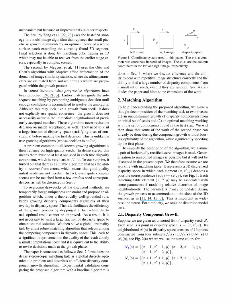
Figure 1. Coordinate system used in this paper. The y is a com-mon row coordinate in rectified images. The x, x′ are the columncoordinates in the left and right image, respectively.

done in Sec. 3, where we discuss efficiency and the abil-ity to deal with repetitive image structures correctly and theability to find a large number of disparity components froma small set of seeds, even if they are random. Sec. 4 con-cludes the paper and hints some extensions of the work.

2. Matching AlgorithmTo help understanding the proposed algorithm, we make athought decomposition of the matching task to two phases:(1) an unconstrained growth of disparity components froman initial set of seeds and (2) an optimal matching workingwith the set of components found in the first step. We willthen show that some of the work of the second phase canalready be done during the component growth without loos-ing optimality of the algorithm, while significantly speedingup the first phase.

To simplify the description of the algorithm, we assumea pair of horizontally rectified stereo images is used. Gener-alization to unrectified images is possible but it will not bediscussed in the present paper. We therefore assume we areworking with matching table. It represents a 3D discretizeddisparity space in which each element (x, x′, y) denotes apossible correspondence (x, y) ↔ (x′, y), see Fig. 1. Eachmatching table element (x, x′, y) may be associated withsome parameters θ modeling relative distortion of imageneighborhoods. The parameters θ may be updated duringthe growth process to accommodate to the slant of the 3Dsurface, as in [11, 14, 13, 7]. This is important in wide-baseline stereo. For simplicity, we omit the distortion modelhere.

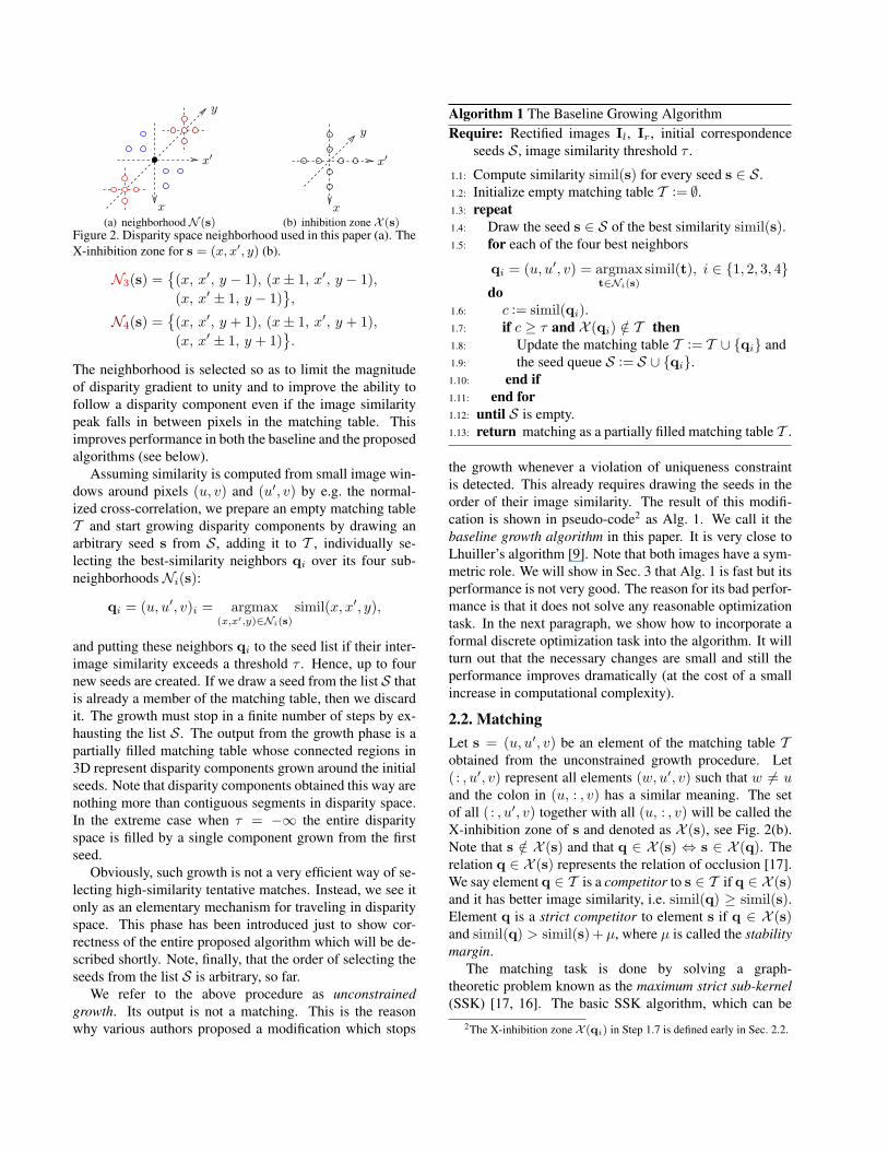
2.1. Disparity Component GrowthSuppose we are given an unsorted list of disparity seeds S.Each seed is a point in disparity space, s = (x, x′, y). Itsneighborhood N (s) in disparity space consists of 16 pointsconstructed from four sub-sets N1(s) ∪ N2(s) ∪ N3(s) ∪N4(s), see Fig. 2(a) where we use the same colors for:

N1(s) ={(x− 1, x′ − 1, y), (x− 2, x′ − 1, y),(x− 1, x′ − 2, y)

},

N2(s) ={(x + 1, x′ + 1, y), (x + 2, x′ + 1, y),(x + 1, x′ + 2, y)

},

x′

x

y

(a) neighborhoodN (s)

x′

x

y

(b) inhibition zone X (s)Figure 2. Disparity space neighborhood used in this paper (a). TheX-inhibition zone for s = (x, x′, y) (b).

N3(s) ={(x, x′, y − 1), (x± 1, x′, y − 1),(x, x′ ± 1, y − 1)

},

N4(s) ={(x, x′, y + 1), (x± 1, x′, y + 1),(x, x′ ± 1, y + 1)

}.

The neighborhood is selected so as to limit the magnitudeof disparity gradient to unity and to improve the ability tofollow a disparity component even if the image similaritypeak falls in between pixels in the matching table. Thisimproves performance in both the baseline and the proposedalgorithms (see below).

Assuming similarity is computed from small image win-dows around pixels (u, v) and (u′, v) by e.g. the normal-ized cross-correlation, we prepare an empty matching tableT and start growing disparity components by drawing anarbitrary seed s from S, adding it to T , individually se-lecting the best-similarity neighbors qi over its four sub-neighborhoods Ni(s):

qi = (u, u′, v)i = argmax(x,x′,y)∈Ni(s)

simil(x, x′, y),

and putting these neighbors qi to the seed list if their inter-image similarity exceeds a threshold τ . Hence, up to fournew seeds are created. If we draw a seed from the list S thatis already a member of the matching table, then we discardit. The growth must stop in a finite number of steps by ex-hausting the list S. The output from the growth phase is apartially filled matching table whose connected regions in3D represent disparity components grown around the initialseeds. Note that disparity components obtained this way arenothing more than contiguous segments in disparity space.In the extreme case when τ = −∞ the entire disparityspace is filled by a single component grown from the firstseed.

Obviously, such growth is not a very efficient way of se-lecting high-similarity tentative matches. Instead, we see itonly as an elementary mechanism for traveling in disparityspace. This phase has been introduced just to show cor-rectness of the entire proposed algorithm which will be de-scribed shortly. Note, finally, that the order of selecting theseeds from the list S is arbitrary, so far.

We refer to the above procedure as unconstrainedgrowth. Its output is not a matching. This is the reasonwhy various authors proposed a modification which stops

Algorithm 1 The Baseline Growing AlgorithmRequire: Rectified images Il, Ir, initial correspondence

seeds S, image similarity threshold τ .

1.1: Compute similarity simil(s) for every seed s ∈ S.1.2: Initialize empty matching table T := ∅.1.3: repeat1.4: Draw the seed s ∈ S of the best similarity simil(s).1.5: for each of the four best neighbors

qi = (u, u′, v) = argmaxt∈Ni(s)

simil(t), i ∈ {1, 2, 3, 4}do

1.6: c := simil(qi).1.7: if c ≥ τ and X (qi) /∈ T then1.8: Update the matching table T := T ∪ {qi} and1.9: the seed queue S := S ∪ {qi}.1.10: end if1.11: end for1.12: until S is empty.1.13: return matching as a partially filled matching table T .

the growth whenever a violation of uniqueness constraintis detected. This already requires drawing the seeds in theorder of their image similarity. The result of this modifi-cation is shown in pseudo-code2 as Alg. 1. We call it thebaseline growth algorithm in this paper. It is very close toLhuiller’s algorithm [9]. Note that both images have a sym-metric role. We will show in Sec. 3 that Alg. 1 is fast but itsperformance is not very good. The reason for its bad perfor-mance is that it does not solve any reasonable optimizationtask. In the next paragraph, we show how to incorporate aformal discrete optimization task into the algorithm. It willturn out that the necessary changes are small and still theperformance improves dramatically (at the cost of a smallincrease in computational complexity).

2.2. MatchingLet s = (u, u′, v) be an element of the matching table Tobtained from the unconstrained growth procedure. Let( : , u′, v) represent all elements (w, u′, v) such that w 6= uand the colon in (u, : , v) has a similar meaning. The setof all ( : , u′, v) together with all (u, : , v) will be called theX-inhibition zone of s and denoted as X (s), see Fig. 2(b).Note that s /∈ X (s) and that q ∈ X (s) ⇔ s ∈ X (q). Therelation q ∈ X (s) represents the relation of occlusion [17].We say element q ∈ T is a competitor to s ∈ T if q ∈ X (s)and it has better image similarity, i.e. simil(q) ≥ simil(s).Element q is a strict competitor to element s if q ∈ X (s)and simil(q) > simil(s) + µ, where µ is called the stabilitymargin.

The matching task is done by solving a graph-theoretic problem known as the maximum strict sub-kernel(SSK) [17, 16]. The basic SSK algorithm, which can be

2The X-inhibition zone X (qi) in Step 1.7 is defined early in Sec. 2.2.

used for our problem class and which we call the domi-nant element reduction algorithm works as follows. Givenmatching table T , partially filled with disparity componentsfrom the unconstrained growth phase, one finds a dominantelement s of the table whose image similarity satisfies

simil(s) > maxt∈X (s)

simil(t) + µ, (1)

where µ is the stability margin. If there was no dominantelement, the algorithm stops. Next, given the dominant el-ement s, one removes all elements X (s) from T . In thereduced table, new dominant element is found and the re-duction process is repeated. The procedure finishes in a fi-nite number of steps. The fully reduced table T contains aset that is the largest (i.e. maximum) one-to-one matchingthat is a SSK. It can be proved that our problem always hasat most one maximum SSK and that the above algorithm isable to find it or confirm there is none [17]. The definingquality of a SSK is its strict stability, which can be consid-ered a global ‘optimality’ property in the following sense:Let T be the set of all elements in the initial matching table.Let K be a subset of T . We say K is strictly stable if for ev-ery p,q ∈ K it holds that p /∈ X (q) (i.e. K is a one-to-onematching) and every element s ∈ K is strictly stable withrespect to K. An element s ∈ K is strictly stable wrt K ifevery competitor q ∈ T to s has a strict competitor t in K.Hence, SSK is the only set that is strictly stable. Note that aSSK can be incomplete. In the extreme case it can be emptyif there was no dominant element. Incompleteness is a nec-essary prerequisite for robustness. See [17] for a discussionof properties of SSK related to robustness.

The paper [17] formulates the SSK problem in rigor-ous graph-theoretical language and should be referred tofor necessary conditions under which the algorithm is valid(for our problem it is valid).3 The above algorithm directlyperforms guiding or the least commitment strategy, as dis-cussed in [24]: most reliable decisions are made prior tounreliable ones that wait until the set of putative solutionsbecomes more constrained.4 The accuracy of stereoscopicmatching based on the SSK is studied in [8].

Besides the dominant element reduction algorithm, thereis another algorithm for finding an SSK, which is moresuitable for our matching problem and which produces anequivalent result [16, 17]. It has two phases: The first phase

3Strict sub-kernel is a general notion valid for oriented graphs, in whichthe graph structure represents the structure of the underlying problem (thestructure of constraints) and the orientation represents evidence (data) [17].The notion of SSK is related to the well-known Stable Marriage and StableRoommates Problems [5].

4Note that the fact the above algorithm proceeds in this way is only dueto the special structure of our matching problem. In more general graphorientations, the SSK algorithm is more complex and the general problemof finding a SSK is NP-complete [17]. It can be shown that when µ = 0the SSK approximates the max-sum independent vertex set problem withina factor of two (in our problem) [17].

runs as in the dominant element reduction algorithm butwith µ = 0 and with the dominance test inequalities notsharp (in such case we are obtaining weakly dominant el-ements). We call its result a weak kernel (WK). It can beshown that maximum SSK is always a subset of a WK, ir-respective of the order of processing the weakly dominantelements [17]. In the second phase, the WK is converted toa maximum SSK as follows:

Require: The output T from unconstrained growth,the WK K ⊆ T .

1: loop2: Find an element q ∈ T , q /∈ K such that

X (q) ∩ K is empty or

simil(q) + µ ≥ maxt∈X (q)∩K

simil(t).

3: if no such q was found then4: return reduced WK K5: else6: Remove q and X (q) from T and K.7: end if8: end loop

The q in Step 2 are called the converting elements. Ob-viously, their neighbors in X (q) ∩ K violate the strong sta-bility condition. Correctness of this algorithm has beenproved [17]. A fast algorithm for simultaneous finding WKand its progressive conversion to SSK, is described in [16].

The formulation given here clearly shows what to do inthe disparity component growth procedure: Instead of stop-ping whenever the uniqueness constraint would be violatedas in Step 1.7 of Alg. 1, we have to continue the growthunless image similarities of the overlapping disparity com-ponents differ more than µ. Hereby, the components thatcannot survive the final competition are not grown further.The resulting modification of Alg. 1 is shown in pseudo-code as Alg. 2. The difference is in Step 2.7 and in someinexpensive bookkeeping in Step 2.10. The difference isseemingly subtle but it has a strong impact on the abilityto reject some of the bad matches, including some of theseeds, as will be shown in Sec. 3.

Of course, the partially filled matching table output fromAlg. 2 is not yet a matching because of the overlap of dis-parity components in matching table T which violates theuniqueness constraint. The overgrown components undergoa competition in a subsequent selection process. To this endthe output from Alg. 2 is processed by the dominant elementreduction algorithm discussed above or by the equivalentWK conversion algorithm. We use an implementation thathas been proposed for semi-dense stereo matching [16] andthat does not require a fully populated matching table. Thisfinal matching is computationally very efficient because ofthe sparsity of T . Our experiments show it takes less than15% of the overall computing time.

Algorithm 2 The Proposed Growing AlgorithmRequire: Rectified images Il, Ir, initial correspondence

seeds S, image similarity threshold τ , and margin µ.

2.1: Compute image similarity for all seeds s ∈ S.2.2: Initialize matching table T := ∅, and auxiliary arrays

Cbest( : , : ) :=−∞, C′best( : , : ) :=−∞.

2.3: repeat2.4: Draw the seed s = (x, x′, y) ∈ S of the best image

similarity simil(s).2.5: for each of the four best neighbors

qi = (u, u′, v) = argmaxt∈Ni(s)

simil(t), i ∈ {1, 2, 3, 4}

do2.6: c := simil(qi).2.7: if c ≥ τ and qi /∈ T and

c + µ ≥ min{Cbest(u, v), C′

best(u′, v)

}then

2.8: Update the matching table T := T ∪ {qi},2.9: the seed queue S := S ∪ {qi},2.10: and the best image similarities

Cbest(u, v) := max{c, Cbest(u, v)

},

C′best(u

′, v) := max{c, C′

best(u′, v)

}.

2.11: end if2.12: end for2.13: until S is empty.2.14: return table T with traced-out disparity components.

2.3. Implementation NotesThe matching table T of Alg. 1 is implemented as two 2Darrays of the input image sizes, each containing a match in-dex to the other image. The second 2D array is needed for afast check of the symmetric uniqueness constraint. The cor-relation map is stored separately. This is possible becausethere is at most one match per pixel.

In the proposed algorithm Alg. 2, the data structure forT is more complicated, since the uniqueness does not holdduring the growth process. The T is very sparse, therefore,it is implemented as a 2D array of binary search trees withdisparities as the keys. Inserting an element and the test onelement’s presence both take logarithmic time.

3. ExperimentsWe first demonstrate the principal differences between thebaseline and the proposed algorithms on synthetic data andthen compare their performance on some real data and on aground-truth dataset.

We use Moravec’s NCC [12] on 5 × 5 window as im-age similarity statistic in all experiments. The default pa-rameters of the algorithms are τ = 0.6, µ = 0.1. Unlessstated otherwise, we use a simple pre-matcher to obtain ini-tial seeds which we call Harris seeds: we take all corre-

(a) left image

(b) baseline (c) proposed

(d) baseline (e) proposed

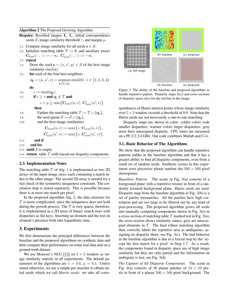
Figure 3. The ability of the baseline and proposed algorithms tohandle repetitive pattern. Disparity maps (b,c) and cross-sectionsof disparity space (d,e) for the red line in the image.

spondences of Harris interest points whose image similarityover 5×5 window exceeds a threshold of 0.9. Note that theHarris seeds are not necessarily a one-to-one matching.

Disparity maps are shown in color: colder colors codesmaller disparities, warmer colors larger disparities, grayareas have unassigned disparity. CPU times are measuredon a PC C2 2.4 GHz. Our code combines Matlab and C++.

3.1. Basic Behavior of The AlgorithmsWe show that the proposed algorithm can handle repetitivepatterns unlike in the baseline algorithm and that it has agreater ability to find all disparity components, even from asmall set of random seeds. Synthetic scenes in this exper-iment were piecewise planar random dot 500 × 500 pixelstereograms.

Repetitive Pattern. The scene in Fig. 3(a) consists of aforeground plane with a repetitive texture in front of a ran-domly textured background plane. Harris seeds are used.Disparity map from the baseline algorithm in Fig. 3(b) is aset of patchy mismatches. All the patches have high cor-relation and are too large to be filtered out by any kind ofpost-processing. The proposed algorithm grows all seedsinto mutually competing components shown in Fig. 3(e) ina cross-section of matching table T marked red in Fig. 3(a),the cross-section shows similarity values, grey are unoccu-pied elements in T . The final robust matching algorithmthen correctly labels the repetitive area as ambiguous, as-signing no disparity there, see Fig. 3(c). The bad behaviorin the baseline algorithm is due to a forced stop by the ‘ac-cept the first match for a pixel’ in Step 1.7. As a result,the components found in disparity space are of high imagesimilarity but they are only partial and the information onambiguity is lost, see Fig. 3(d).

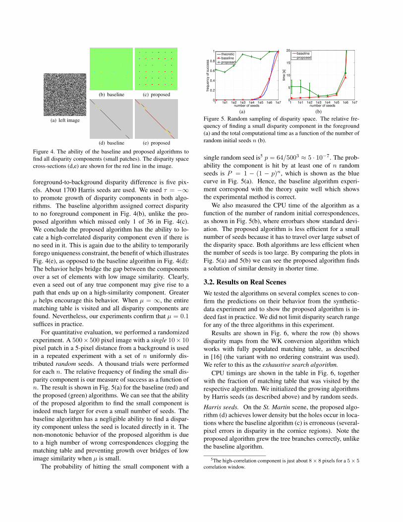
The Capture of All Disparity Components. The scene inFig. 4(a) consists of 36 planar patches of 10 × 10 pix-els in front of a planar 500 × 500 pixel background. The

(a) left image

(b) baseline (c) proposed

(d) baseline (e) proposed

Figure 4. The ability of the baseline and proposed algorithms tofind all disparity components (small patches). The disparity spacecross-sections (d,e) are shown for the red line in the image.

foreground-to-background disparity difference is five pix-els. About 1700 Harris seeds are used. We used τ = −∞to promote growth of disparity components in both algo-rithms. The baseline algorithm assigned correct disparityto no foreground component in Fig. 4(b), unlike the pro-posed algorithm which missed only 1 of 36 in Fig. 4(c).We conclude the proposed algorithm has the ability to lo-cate a high-correlated disparity component even if there isno seed in it. This is again due to the ability to temporarilyforego uniqueness constraint, the benefit of which illustratesFig. 4(e), as opposed to the baseline algorithm in Fig. 4(d):The behavior helps bridge the gap between the componentsover a set of elements with low image similarity. Clearly,even a seed out of any true component may give rise to apath that ends up on a high-similarity component. Greaterµ helps encourage this behavior. When µ = ∞, the entirematching table is visited and all disparity components arefound. Nevertheless, our experiments confirm that µ = 0.1suffices in practice.

For quantitative evaluation, we performed a randomizedexperiment. A 500× 500 pixel image with a single 10× 10pixel patch in a 5-pixel distance from a background is usedin a repeated experiment with a set of n uniformly dis-tributed random seeds. A thousand trials were performedfor each n. The relative frequency of finding the small dis-parity component is our measure of success as a function ofn. The result is shown in Fig. 5(a) for the baseline (red) andthe proposed (green) algorithms. We can see that the abilityof the proposed algorithm to find the small component isindeed much larger for even a small number of seeds. Thebaseline algorithm has a negligible ability to find a dispar-ity component unless the seed is located directly in it. Thenon-monotonic behavior of the proposed algorithm is dueto a high number of wrong correspondences clogging thematching table and preventing growth over bridges of lowimage similarity when µ is small.

The probability of hitting the small component with a

1 1e1 1e2 1e3 1e4 1e5 1e6 1e70

0.2

0.4

0.6

0.8

1

number of seeds

fre

qu

en

cy o

f su

cce

ss

theoretic

baselineproposed

(a)

1 1e1 1e2 1e3 1e4 1e5 1e6 1e70

5

10

15

20

number of seeds

tim

e [s]

baselineproposed

(b)Figure 5. Random sampling of disparity space. The relative fre-quency of finding a small disparity component in the foreground(a) and the total computational time as a function of the number ofrandom initial seeds n (b).

single random seed is5 p = 64/5003 ≈ 5 · 10−7. The prob-ability the component is hit by at least one of n randomseeds is P = 1 − (1 − p)n, which is shown as the bluecurve in Fig. 5(a). Hence, the baseline algorithm experi-ment correspond with the theory quite well which showsthe experimental method is correct.

We also measured the CPU time of the algorithm as afunction of the number of random initial correspondences,as shown in Fig. 5(b), where errorbars show standard devi-ation. The proposed algorithm is less efficient for a smallnumber of seeds because it has to travel over large subset ofthe disparity space. Both algorithms are less efficient whenthe number of seeds is too large. By comparing the plots inFig. 5(a) and 5(b) we can see the proposed algorithm findsa solution of similar density in shorter time.

3.2. Results on Real ScenesWe tested the algorithms on several complex scenes to con-firm the predictions on their behavior from the synthetic-data experiment and to show the proposed algorithm is in-deed fast in practice. We did not limit disparity search rangefor any of the three algorithms in this experiment.

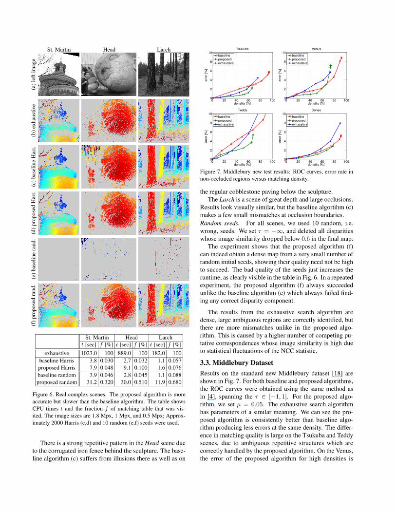
Results are shown in Fig. 6, where the row (b) showsdisparity maps from the WK conversion algorithm whichworks with fully populated matching table, as describedin [16] (the variant with no ordering constraint was used).We refer to this as the exhaustive search algorithm.

CPU timings are shown in the table in Fig. 6, togetherwith the fraction of matching table that was visited by therespective algorithm. We initialized the growing algorithmsby Harris seeds (as described above) and by random seeds.

Harris seeds. On the St. Martin scene, the proposed algo-rithm (d) achieves lower density but the holes occur in loca-tions where the baseline algorithm (c) is erroneous (several-pixel errors in disparity in the cornice regions). Note theproposed algorithm grew the tree branches correctly, unlikethe baseline algorithm.

5The high-correlation component is just about 8× 8 pixels for a 5× 5correlation window.

St. Martin Head Larch

(a)l

efti

mag

e(b

)exh

aust

ive

(c)b

asel

ine

Har

r.(d

)pro

pose

dH

arr.

(e)b

asel

ine

rand

.(f

)pro

pose

dra

nd.

St. Martin Head Larcht [sec] f [%] t [sec] f [%] t [sec] f [%]

exhaustive 1023.0 100 889.0 100 182.0 100baseline Harris 3.8 0.030 2.7 0.032 1.1 0.057proposed Harris 7.9 0.048 9.1 0.100 1.6 0.076baseline random 3.9 0.046 2.8 0.045 1.1 0.088proposed random 31.2 0.320 30.0 0.510 11.9 0.680

Figure 6. Real complex scenes. The proposed algorithm is moreaccurate but slower than the baseline algorithm. The table showsCPU times t and the fraction f of matching table that was vis-ited. The image sizes are 1.8 Mpx, 1 Mpx, and 0.5 Mpx; Approx-imately 2000 Harris (c,d) and 10 random (e,f) seeds were used.

There is a strong repetitive pattern in the Head scene dueto the corrugated iron fence behind the sculpture. The base-line algorithm (c) suffers from illusions there as well as on

0 20 40 60 80 1000

2

4

6

8

10

denstity [%]

err

or

[%]

Tsukuba

baseline

proposed

exhaustive

0 20 40 60 80 1000

2

4

6

8

10

denstity [%]

err

or

[%]

Venus

baseline

proposed

exhaustive

0 20 40 60 80 1000

2

4

6

8

10

denstity [%]

err

or

[%]

Teddy

baseline

proposed

exhaustive

0 20 40 60 80 1000

2

4

6

8

10

denstity [%]

err

or

[%]

Cones

baselineproposedexhaustive

Figure 7. Middlebury new test results: ROC curves, error rate innon-occluded regions versus matching density.

the regular cobblestone paving below the sculpture.The Larch is a scene of great depth and large occlusions.

Results look visually similar, but the baseline algortihm (c)makes a few small mismatches at occlusion boundaries.Random seeds. For all scenes, we used 10 random, i.e.wrong, seeds. We set τ = −∞, and deleted all disparitieswhose image similarity dropped below 0.6 in the final map.

The experiment shows that the proposed algorithm (f)can indeed obtain a dense map from a very small number ofrandom initial seeds, showing their quality need not be highto succeed. The bad quality of the seeds just increases theruntime, as clearly visible in the table in Fig. 6. In a repeatedexperiment, the proposed algorithm (f) always succeededunlike the baseline algorithm (e) which always failed find-ing any correct disparity component.

The results from the exhaustive search algorithm aredense, large ambiguous regions are correctly identified, butthere are more mismatches unlike in the proposed algo-rithm. This is caused by a higher number of competing pu-tative correspondences whose image similarity is high dueto statistical fluctuations of the NCC statistic.

3.3. Middlebury DatasetResults on the standard new Middlebury dataset [18] areshown in Fig. 7. For both baseline and proposed algorithms,the ROC curves were obtained using the same method asin [4], spanning the τ ∈ [−1, 1]. For the proposed algo-rithm, we set µ = 0.05. The exhaustive search algorithmhas parameters of a similar meaning. We can see the pro-posed algorithm is consistently better than baseline algo-rithm producing less errors at the same density. The differ-ence in matching quality is large on the Tsukuba and Teddyscenes, due to ambiguous repetitive structures which arecorrectly handled by the proposed algorithm. On the Venus,the error of the proposed algorithm for high densities is

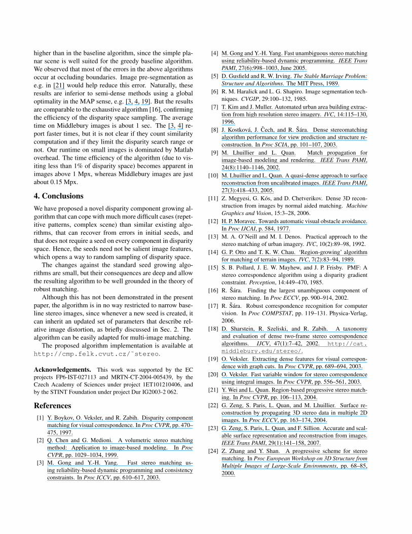
higher than in the baseline algorithm, since the simple pla-nar scene is well suited for the greedy baseline algorithm.We observed that most of the errors in the above algorithmsoccur at occluding boundaries. Image pre-segmentation ase.g. in [21] would help reduce this error. Naturally, theseresults are inferior to semi-dense methods using a globaloptimality in the MAP sense, e.g. [3, 4, 19]. But the resultsare comparable to the exhaustive algorithm [16], confirmingthe efficiency of the disparity space sampling. The averagetime on Middlebury images is about 1 sec. The [3, 4] re-port faster times, but it is not clear if they count similaritycomputation and if they limit the disparity search range ornot. Our runtime on small images is dominated by Matlaboverhead. The time efficiency of the algorithm (due to vis-iting less than 1% of disparity space) becomes apparent inimages above 1 Mpx, whereas Middlebury images are justabout 0.15 Mpx.

4. ConclusionsWe have proposed a novel disparity component growing al-gorithm that can cope with much more difficult cases (repet-itive patterns, complex scene) than similar existing algo-rithms, that can recover from errors in initial seeds, andthat does not require a seed on every component in disparityspace. Hence, the seeds need not be salient image features,which opens a way to random sampling of disparity space.

The changes against the standard seed growing algo-rithms are small, but their consequences are deep and allowthe resulting algorithm to be well grounded in the theory ofrobust matching.

Although this has not been demonstrated in the presentpaper, the algorithm is in no way restricted to narrow base-line stereo images, since whenever a new seed is created, itcan inherit an updated set of parameters that describe rel-ative image distortion, as briefly discussed in Sec. 2. Thealgorithm can be easily adapted for multi-image matching.

The proposed algorithm implementation is available athttp://cmp.felk.cvut.cz/˜stereo.

Acknowledgements. This work was supported by the ECprojects FP6-IST-027113 and MRTN-CT-2004-005439, by theCzech Academy of Sciences under project 1ET101210406, andby the STINT Foundation under project Dur IG2003-2 062.

References[1] Y. Boykov, O. Veksler, and R. Zabih. Disparity component

matching for visual correspondence. In Proc CVPR, pp. 470–475, 1997.

[2] Q. Chen and G. Medioni. A volumetric stereo matchingmethod: Application to image-based modeling. In ProcCVPR, pp. 1029–1034, 1999.

[3] M. Gong and Y.-H. Yang. Fast stereo matching us-ing reliability-based dynamic programming and consistencyconstraints. In Proc ICCV, pp. 610–617, 2003.

[4] M. Gong and Y.-H. Yang. Fast unambiguous stereo matchingusing reliability-based dynamic programming. IEEE TransPAMI, 27(6):998–1003, June 2005.

[5] D. Gusfield and R. W. Irving. The Stable Marriage Problem:Structure and Algorithms. The MIT Press, 1989.

[6] R. M. Haralick and L. G. Shapiro. Image segmentation tech-niques. CVGIP, 29:100–132, 1985.

[7] T. Kim and J. Muller. Automated urban area building extrac-tion from high resolution stereo imagery. IVC, 14:115–130,1996.

[8] J. Kostkova, J. Cech, and R. Sara. Dense stereomatchingalgorithm performance for view prediction and structure re-construction. In Proc SCIA, pp. 101–107, 2003.

[9] M. Lhuillier and L. Quan. Match propagation forimage-based modeling and rendering. IEEE Trans PAMI,24(8):1140–1146, 2002.

[10] M. Lhuillier and L. Quan. A quasi-dense approach to surfacereconstruction from uncalibrated images. IEEE Trans PAMI,27(3):418–433, 2005.

[11] Z. Megyesi, G. Kos, and D. Chetverikov. Dense 3D recon-struction from images by normal aided matching. MachineGraphics and Vision, 15:3–28, 2006.

[12] H. P. Moravec. Towards automatic visual obstacle avoidance.In Proc IJCAI, p. 584, 1977.

[13] M. A. O’Neill and M. I. Denos. Practical approach to thestereo matching of urban imagery. IVC, 10(2):89–98, 1992.

[14] G. P. Otto and T. K. W. Chau. ‘Region-growing’ algorithmfor matching of terrain images. IVC, 7(2):83–94, 1989.

[15] S. B. Pollard, J. E. W. Mayhew, and J. P. Frisby. PMF: Astereo correspondence algorithm using a disparity gradientconstraint. Perception, 14:449–470, 1985.

[16] R. Sara. Finding the largest unambiguous component ofstereo matching. In Proc ECCV, pp. 900–914, 2002.

[17] R. Sara. Robust correspondence recognition for computervision. In Proc COMPSTAT, pp. 119–131. Physica-Verlag,2006.

[18] D. Sharstein, R. Szeliski, and R. Zabih. A taxonomyand evaluation of dense two-frame stereo correspondencealgorithms. IJCV, 47(1):7–42, 2002. http://cat.middlebury.edu/stereo/.

[19] O. Veksler. Extracting dense features for visual correspon-dence with graph cuts. In Proc CVPR, pp. 689–694, 2003.

[20] O. Veksler. Fast variable window for stereo correspondenceusing integral images. In Proc CVPR, pp. 556–561, 2003.

[21] Y. Wei and L. Quan. Region-based progressive stereo match-ing. In Proc CVPR, pp. 106–113, 2004.

[22] G. Zeng, S. Paris, L. Quan, and M. Lhuillier. Surface re-construction by propagating 3D stereo data in multiple 2Dimages. In Proc ECCV, pp. 163–174, 2004.

[23] G. Zeng, S. Paris, L. Quan, and F. Sillion. Accurate and scal-able surface representation and reconstruction from images.IEEE Trans PAMI, 29(1):141–158, 2007.

[24] Z. Zhang and Y. Shan. A progressive scheme for stereomatching. In Proc European Workshop on 3D Structure fromMultiple Images of Large-Scale Environments, pp. 68–85,2000.