Speeded-up, relaxed spatial matching

Giorgos Tolias and Yannis AvrithisNational Technical University of Athens

{gtolias,iavr}@image.ntua.gr

Abstract

A wide range of properties and assumptions determinethe most appropriate spatial matching model for an ap-plication, e.g. recognition, detection, registration, or largescale image retrieval. Most notably, these include discrim-inative power, geometric invariance, rigidity constraints,mapping constraints, assumptions made on the underlyingfeatures or descriptors and, of course, computational com-plexity. Having image retrieval in mind, we present a verysimple model inspired by Hough voting in the transforma-tion space, where votes arise from single feature correspon-dences. A relaxed matching process allows for multiplematching surfaces or non-rigid objects under one-to-onemapping, yet is linear in the number of correspondences. Weapply it to geometry re-ranking in a search engine, yieldingsuperior performance with the same space requirements buta dramatic speed-up compared to the state of the art.

1. IntroductionDiscriminative local features have made sub-linear index-ing of appearance possible, but geometry indexing still ap-pears elusive if one targets invariance, global geometry ver-ification, high precision and low space requirements. Largescale image retrieval solutions typically consider geometryin a second, re-ranking phase. The latter is linear in thenumber of images to match, hence its speed is crucial.

Exploiting local shape of features (e.g. local scale, ori-entation, or affine parameters) to extrapolate relative trans-formations, it is either possible to construct RANSAC hy-potheses by single correspondences [14], or to see corre-spondences as Hough votes in a transformation space [12].In the former case one still has to count inliers, so the pro-cess is quadratic in the number of (tentative) correspon-dences. In the latter, voting is linear but further verificationwith inlier count seems unavoidable.

Flexible spatial models are more typical in recognition;these are either not invariant to geometric transformations,or use pairwise constraints to detect inliers without anyrigid motion model [11]. The latter are at least quadratic

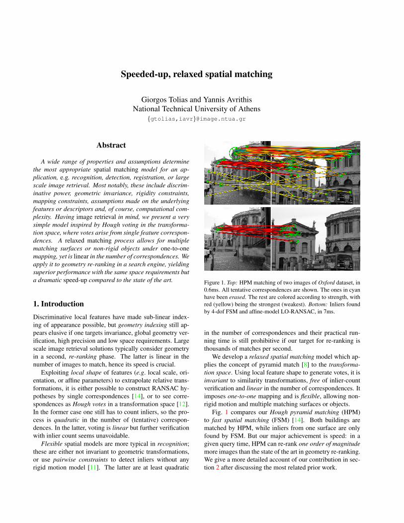
Figure 1. Top: HPM matching of two images of Oxford dataset, in0.6ms. All tentative correspondences are shown. The ones in cyanhave been erased. The rest are colored according to strength, withred (yellow) being the strongest (weakest). Bottom: Inliers foundby 4-dof FSM and affine-model LO-RANSAC, in 7ms.

in the number of correspondences and their practical run-ning time is still prohibitive if our target for re-ranking isthousands of matches per second.

We develop a relaxed spatial matching model which ap-plies the concept of pyramid match [8] to the transforma-tion space. Using local feature shape to generate votes, it isinvariant to similarity transformations, free of inlier-countverification and linear in the number of correspondences. Itimposes one-to-one mapping and is flexible, allowing non-rigid motion and multiple matching surfaces or objects.

Fig. 1 compares our Hough pyramid matching (HPM)to fast spatial matching (FSM) [14]. Both buildings arematched by HPM, while inliers from one surface are onlyfound by FSM. But our major achievement is speed: in agiven query time, HPM can re-rank one order of magnitudemore images than the state of the art in geometry re-ranking.We give a more detailed account of our contribution in sec-tion 2 after discussing the most related prior work.

2. Related work and contributionGiven a number of correspondences between a pair of im-ages, RANSAC [7] is still one of the most popular geomet-ric verification models. However, its performance is poorwhen the ratio of inliers is too low. Philbin et al. [14] gener-ate hypotheses from single correspondences exploiting lo-cal feature shape. Matching then becomes deterministic byenumerating all hypotheses. Still, this process is quadraticin the number of correspondences.

Consistent groups of correspondences may first be foundin the transformation space using the generalized Houghtransform [3]. This is carried out by Lowe [12], but onlyas a prior step to verification. Tentative correspondencesare found via fast nearest neighbor search in the descrip-tor space and used to generate votes in the transformationspace. Performance depends on the number rather than theratio of inliers. Still, multiple groups need to be verified forinliers and this may be quadratic in the worst case.

Jegou et al. use a weaker geometric model [9] wheregroups of correspondences only agree in their relativescale and—independently—orientation. Correspondencesare found using a visual codebook. Scale and orientation oflocal features are quantized and stored in the inverted file.Hence, weak geometric constraints are integrated in the fil-tering stage of the search engine. However, this model doesnot dispense with geometry re-ranking after all.

More flexible models are typically used for recogni-tion. For instance, multiple groups of consistent correspon-dences are identified with the flexible, semi-local modelof Carneiro and Jepson [5], employing pairwise relationsbetween correspondences and allowing non-rigid deforma-tions. Similarly, Leordeanu and Hebert [11] build a sparseadjacency (affinity) matrix of correspondences and greed-ily recover inliers based on its principal eigenvector. Thisspectral model can additionally incorporate different featuremapping constraints like one-to-one.

One-to-one mapping is maybe reminiscent of early cor-respondence methods on non-discriminative features, butcan be very important when codebooks are small, under thepresence of repeating structures, or e.g. with soft assign-ment models like Philbin et al. [15]. Most flexible modelsare iterative and at least quadratic in the number of corre-spondences.

Relaxed matching processes like Vedaldi and Soatto [18]offer an extremely attractive alternative in terms of com-plexity by employing distributions over hierarchical parti-tions instead of pairwise computations. The most popularis by Grauman and Darell [8], who map features to a multi-resolution histogram in the descriptor space, and then matchthem in a bottom-up process. The benefit comes mainlyfrom approximating similarities by bin size. Lazebnik etal. [10] apply the same idea to image space but in such away that geometric invariance is lost.

Contribution. While the above relaxed methods applyto two sets of features, we rather apply the same idea to oneset of correspondences (feature pairs) and aim at groupingaccording to proximity, or affinity. This problem resem-bles mode seeking [17], but our solution is a non-iterative,bottom-up grouping process that is free of any scale pa-rameter. We represent correspondences in the transforma-tion space exploiting local feature shape as in [12], butwe form correspondences using a codebook. Like pyramidmatch [8], we approximate affinity by bin size, without ac-tually enumerating correspondence pairs.

We also impose an one-to-one mapping constraint suchthat each feature in one image is mapped to at most one fea-ture in the other. Indeed, this makes our problem similarto that of [11], in the sense that we greedily select a pair-wise compatible subset of correspondences that maximize anon-negative, symmetric affinity matrix. However we allowmultiple groups (clusters) of correspondences.

To summarize, we derive a flexible spatial matchingscheme where all tentative correspondences contribute, ap-propriately weighted, to a similarity score. What is most re-markable is that no verification, model fitting or inlier countis needed as in [12], [14] or [5]. Besides significant perfor-mance gain, this yields a dramatic speed-up. Our result is avery simple algorithm that requires no learning and can beeasily integrated into any image retrieval process.

3. Problem formulation

We assume an image is represented by a set P of local fea-tures, and for each feature p ∈ P we are given its descriptor,position and local shape. We restrict discussion to scale androtation covariant features, so that the local shape and posi-tion of feature p are given by the 3× 3 matrix

F (p) =

[M(p) t(p)0T 1

], (1)

where M(p) = σ(p)R(p) and σ(p), R(p), t(p) stand forisotropic scale, orientation and position, respectively. R(p)is an orthogonal 2 × 2 matrix with detR(p) = 1, repre-sented by an angle θ(p). In effect, F (p) specifies a similar-ity transformation w.r.t. a normalized patch e.g. centered atthe origin with scale σ0 = 1 and orientation θ0 = 0.

Given two images P,Q, an assignment or correspon-dence c = (p, q) is a pair of features p ∈ P, q ∈ Q. The rel-ative transformation from p to q is again a similarity trans-formation given by

F (c) = F (q)F (p)−1 =

[M(c) t(c)0T 1

], (2)

where M(c) = σ(c)R(c), t(c) = t(q) − M(c)t(p); andσ(c) = σ(q)/σ(p), R(c) = R(q)R(p)−1 are the relative

scale and orientation respectively from p to q. This is a 4-dof transformation represented by a parameter vector

f(c) = (x(c), y(c), σ(c), θ(c)), (3)

where [x(c) y(c)]T = t(c) and θ(c) = θ(q) − θ(p). Henceassignments can be seen as points in a d-dimensional trans-formation space F with d = 4 in our case.

An initial set C of candidate or tentative correspon-dences is constructed according to proximity of features inthe descriptor space. Here we consider the simplest visualcodebook approach where two features correspond whenassigned to the same visual word:

C = {(p, q) ∈ P ×Q : u(p) = u(q)}, (4)

where u(p) is the codeword, or visual word, of p. This is amany-to-many mapping; each feature in P may have mul-tiple assignments to features in Q, and vice versa. Givenassignment c = (p, q), we define its visual word u(c) as thecommon visual word u(p) = u(q).

Each correspondence c = (p, q) ∈ C is given a weightw(c) measuring its relative importance; we typically use theinverse document frequency (idf ) of its visual word. Givena pair of assignments c, c′ ∈ C, we assume an affinity scoreα(c, c′) measures their similarity as a non-increasing func-tion of their distance in the transformation space. Finally,we say that two assignments c = (p, q), c′ = (p′, q′) arecompatible if p 6= p′ and q 6= q′, and conflicting otherwise.For instance, c, c′ are conflicting if they are mapping twofeatures of P to the same feature of Q.

Our problem is then to identify a subset of pairwise com-patible assignments that maximizes the total weighted, pair-wise affinity. This is a binary quadratic programming prob-lem and we only target a very fast, approximate solution.

4. Hough Pyramid MatchingWe assume that transformation parameters may be normal-ized or non-linearly mapped to [0, 1] (see section 5). Hencethe transformation space is F = [0, 1]d. We construct a hi-erarchical partition B = {B0, . . . , BL−1} of F into L lev-els. Each B` ∈ B partitions F into 2kd bins (hypercubes),where k = L − 1 − `. The bins are obtained by uniformlyquantizing each parameter, or partitioning each dimensioninto 2k equal intervals of length 2−k. B0 is at the finest(bottom) level; BL−1 is at the coarsest (top) level and has asingle bin. Each partition B` is a refinement of B`+1.

Starting with the set C of tentative correspondences ofimages P,Q, we distribute correspondences into bins witha histogram pyramid. Given a bin b, let

h(b) = {c ∈ C : f(c) ∈ b} (5)

be the set of correspondences with parameter vectors fallinginto b, and |h(b)| its count.

4.1. Matching process

We recursively split correspondences into bins in a top-down fashion, and then group them again recursively in abottom-up fashion. We expect to find most groups of con-sistent correspondences at the finest (bottom) levels, but wedo go all the way up the hierarchy to account for flexibil-ity. Large groups of correspondences formed at a fine levelare more likely to be true, or inliers. It follows that eachcorrespondence should contribute to the similarity score ac-cording to the size of the groups it participates in and thelevel at which these groups were formed.

In order to impose a one-to-one mapping constraint, wedetect conflicting correspondences at each level and greed-ily choose the best one to keep on our way up the hierarchy.The remaining are marked as erased. Let X` denote the setof all erased correspondences up to level `. If b ∈ B` is abin at level `, then the set of correspondences we have keptin b is h(b) = h(b) \X`. Clearly, a single correspondencein a bin does not make a group, while each correspondencelinks to m − 1 other correspondences in a group of m form > 1. Hence we define the group count of bin b as

g(b) = max{0, |h(b)| − 1}. (6)

Now, let b0 ⊆ . . . ⊆ b` be the sequence of bins con-taining a correspondence c at successive levels up to level` such that bk ∈ Bk for k = 0, . . . , `. For each k, we ap-proximate the affinity α(c, c′) of c to any other correspon-dence c′ ∈ bk by a fixed quantity. This quantity is assumeda non-negative, non-increasing level affinity function of k,say α(k). We focus here on the decreasing exponential formα(k) = 2−k, such that affinity is inversely proportional tobin size. On the other hand, there are g(bk)− g(bk−1) newcorrespondences joining c in a group at level k. Similarly to[8], this gives rise to the strength of c up to level `:

s`(c) = g(b0) +∑k=1

2−k{g(bk)− g(bk−1)}. (7)

We are now in position to define the similarity score be-tween images P,Q. Indeed, the total strength of c is simplyits strength at the top level, s(c) = sL−1(c). Then, exclud-ing all erased assignments X = XL−1 and taking weightsinto account, we define the similarity score by

s(C) =∑

c∈C\X

w(c)s(c). (8)

On the other hand, we are also in position to choose thebest correspondence in case of conflicts and impose one-to-one mapping. In particular, let c = (p, q), c′ = (p′, q′)be two conflicting assignments. By definition (4), all fourfeatures p, p′, q, q′ share the same visual word, so c, c′ areof equal weight: w(c) = w(c′). Now let b ∈ B` be the

c1

c2c3

c4c5

c6

c7

c8

c9

Level 0

c1

c2c3

c4c5

c6

c7

c8

c9

Level 1

c1

c2c3

c4c5

c6

c7

c8

c9

Level 2

Figure 2. Matching of 9 assignments on a 3-level pyramid in 2D space. Colors denote visual words, and edge strength denotes affinity. Thedotted line between c6, c9 denotes a group that is formed at level 0 and then broken up at level 2, since c6 is erased.

p q similarity score

c1 (2 + 122 + 1

42)w(c1)

c2 (2 + 122 + 1

42)w(c2)

c3 (2 + 122 + 1

42)w(c3)

c4 (1 + 123 + 1

42)w(c4)

c5 (1 + 123 + 1

42)w(c5)

c6 0

c7 0

c8146w(c8)

c9146w(c9)

Figure 3. Assignment labels, features and scores referring toFig. 2. Here vertices and edges denote features (in images P,Q)and assignments, respectively. Assignments c5, c6 are conflicting,being of the form (p, q), (p, q′). Similarly for c7, c8. Assignmentsc1, . . . , c5 join groups at level 0; c8, c9 at level 2; and c6, c7 areerased.

first (finest) bin in the hierarchy with c, c′ ∈ b. It then fol-lows from (7) and (8) that their contribution to the similarityscore may only differ up to level `−1. We therefore choosethe strongest one up to level `− 1 according to (7). In caseof equal strength, or at level 0, we pick one at random.

4.2. Examples and discussion

A toy example is illustrated in Fig. 2, 3, 4. We assume as-signments are conflicting when they share the same visualword. Fig. 2 shows three groups of assignments at level 0:{c1, c2, c3}, {c4, c5} and {c6, c9}. The first two are joinedat level 1. Assignments c7, c8 are conflicting, and c7 iserased at random. Assignments c5, c6 are also conflicting,but are only compared at level 2 where they share the samebin; according to (7), c5 is stronger as it participates in agroup of 5. Hence group {c6, c9} is broken up, c6 is erasedand c8, c9 join c1, . . . , c5 in a group of 7 at level 2.

Apart from the feature/assignment configuration in im-ages P,Q, Fig. 3 also illustrates how the similarity score

c1

c1

c2

c2

c3

c3

c4

c4

c5

c5

c8

c8

c9

c9

c6

c6

c7

c7

1

112

12

14

14

0

0

Figure 4. Affinity matrix equivalent to the strengths of Fig. 3 ac-cording to (7). Assignments have been rearranged so that groupsappear in contiguous blocks. Groups formed at levels 0, 1, 2 areassigned affinity 1, 1

2, 14

respectively. The similarity scores ofFig. 3 may be obtained by summing affinities over rows and mul-tiplying by assignment weights.

of (8) is formed from individual assignment strengths. Forinstance, assignments c1, . . . , c5 have strength contributionsfrom all 3 levels, while c8, c9 only from level 2. Fig. 4shows how these contributions are arranged in an n × naffinity matrix A. In fact, the sum over a row of A equalsthe strength of the corresponding assignment—the diago-nal is excluded due to (6). The upper triangular part of A,responsible for half the similarity score of (8), correspondsto the set of edges among assignments shown in Fig. 2, theedge strength being proportional to affinity. This reveals thepairwise nature of the approach [5][11].

Another example is that of Fig. 1, where we match tworeal images of the same scene from different viewpoints.It is clear that the strongest correspondences, contributingmost to the similarity score, are true inliers. The scene ge-ometry is such that not even a homography can capture themotion of all visible surfaces. Fig. 5 illustrates matching ofassignments in the Hough space. Observe how assignmentsget stronger by grouping according to proximity.

−1.5 −1 −0.5 0 0.5 1 1.5−1.5

−1

−0.5

0

0.5

1

1.5

horizontal translation, x

vert

ical

tran

slat

ion,y

assignmenterased

Figure 5. Correspondences of the example in Fig. 1 as votes in4D transformation space. One 2D projection is depicted, namelytranslation (x, y). Translation is normalized by maximum imagedimension. There are L = 5 levels and we are zooming into thecentral 8×8 bins. Edges represent links between assignments thatare grouped in levels 0, 1, 2 only. Level affinity α is represented bythree tones of gray with black corresponding to α(0) = 1.

4.3. The algorithm

The matching process is outlined more formally in algo-rithm 1. It follows a recursive implementation: code beforethe recursive call of line 12 is associated to the top-downsplitting process, while after that to bottom-up grouping.

Assignment of correspondences to bins is linear-time in|C| in line 11. B` partitions F for each level `, so givena correspondence c there is a unique bin b ∈ B` such thatf(c) ∈ b. We then define a constant-time mapping β` : c 7→b by quantizing parameter vector f(c) to level `. Storage inbins is sparse and linear-space in |C|; complete partitionsB` are never really constructed.

Given a set of assignments in a bin, optimal detection ofconflicts can be a hard problem. In function ERASE, we fol-low a very simple approximation whereby two assignmentsare conflicting when they share the same visual word. Thisavoids storing features; and makes sense because with a finecodebook, features are uniquely mapped to visual words(e.g. 92% in our test sets). For all assignments h(b) of bin bwe first construct the set U of common visual words. Thenwe only keep the strongest assignment of each codewordu ∈ U , erase the rest and update X .

Computation of strengths in lines 17-18 can be shown tobe equivalent to (7). It is clear that all operations in eachrecursive call on bin b are linear in |h(b)|. Since B` parti-tions F for all `, the total operations per level are linear inn = |C|. Hence the time complexity of HPM is O(nL).

Algorithm 1 Hough Pyramid Matching1: procedure HPM(assignments C, levels L)2: X ← ∅; B ← PARTITION(L) . erased; partition3: for all c ∈ C do s(c)← 0 . strengths4: HPM-REC(C,L− 1) . recurse at top5: return score

∑c∈C\X w(c)s(c) . see (8)

6: end procedure7:8: procedure HPM-REC(assignments C, level `)9: if |C| < 2 ∨ ` < 0 return

10: for all b ∈ B` do h(b)← ∅ . histogram11: for all c ∈ C do h(β`(c))← h(β`(c)) ∪ c . quantize12: for all b ∈ B` do HPM-REC(h(b), `− 1) . recurse down13: for all b ∈ B` do14: X ← X∪ ERASE(h(b))15: h(b)← h(b) \X . exclude erased16: if |h(b)| < 2 continue . exclude isolated17: if ` = L− 1 then a← 2 else a← 118: for all c ∈ h(b) do s(c)← s(c) + a2−`|h(b)| . (7)19: end for20: end procedure

5. Implementation

Indexing and re-ranking. HPM turns out to be so fastthat we use it to perform geometric re-ranking in an im-age retrieval engine. We construct an inverted file indexedby visual word and for each feature in the database we storequantized location, scale, orientation and image id. Givena query, this information is sufficient to perform filteringeither by bag of words (BoW) [16] or weak geometric con-sistency (WGC) [9]. A number of top-ranking images aremarked for re-ranking. For each query feature, we retrieveassignments from the inverted file once more, but now onlyfor marked images. For each assignment c found, we com-pute the parameter vector f(c) and store it in a collectionindexed by marked image id. We then match each markedimage to the query using HPM. Finally, we normalize scoresby marked image BoW `2 norm and re-rank.

Quantization. We treat each relative transformationparameter x, y, σ, θ separately—see (3). Translation t(c)in (2) refers to the coordinate frame of the query image,Q. If r is the maximum dimension of Q, we only keep as-signments with translation x, y ∈ [−3r, 3r]. We also filterassignments such that σ ∈ [1/σm, σm], where σm = 10 isabove the range of any feature detector. We compute log-arithmic scale, normalize all ranges to [0, 1] and quantizeparameters uniformly. We also quantize local feature pa-rameters: with 5 levels, each parameter is quantized into 16bins. Our space requirements per feature, as summarized inTable 1, are then exactly the same as in [9]. Query featureparameters are not quantized.

Orientation prior. Because most images on the webare either portrait or landscape, previous methods use prior

image id x y log σ θ total16 4 4 4 4 32

Table 1. Inverted file memory usage per local feature, in bits. Weuse run-length encoding for image id, so 2 bytes are sufficient.

knowledge for relative orientation in their model [14][9].We use the prior of WGC in our model by incorporating theweighting function of [9] in the form of additional weightsin the sum of (8).

6. ExperimentsIn this section we evaluate HPM against state of the art fastspatial matching (FSM) [14] in pairwise matching and in re-ranking in large scale search. In the latter case, we experi-ment on two filtering models, namely baseline bag-of-words(BoW) [16] and weak geometric consistency (WGC) [9].

6.1. Experimental setup

Datasets. We experiment on two publicly availabledatasets, namely Oxford Buildings [14] and Paris [15], andon our own World Cities dataset1. The latter is downloadedfrom Flickr and consists of 927 annotated photos taken inBarcelona city center and 2 million images from 38 citiesto use as a distractor set. The annotated photos are dividedinto 17 groups, each depicting the same building or scene.We have selected 5 queries from each group, making a to-tal of 85 queries for evaluation. We refer to Oxford Build-ings, Paris and our annotated dataset as test sets. Our WorldCities distractors set mostly depict urban scenes exactly likethe test sets, but from different cities.

Features and codebooks. We extract SURF featuresand descriptors [4] from each image, setting strength thresh-old to 2.0 for the detector. We build codebooks with approx-imate k-means (AKM) [14] and we mostly use a genericcodebook of size 100K constructed from a subset of the 2Mdistractors. However, we also employ specific codebooks ofdifferent sizes constructed from the test sets. Unless other-wise stated, we use the generic codebook.

6.2. Matching experiment

Enumerating all possible image pairs of World Cities testset, there are 74, 075 pairs of images depicting the samebuilding or scene. The similarity score should be high forthose pairs and low for the remaining 785, 254; we thereforeapply different thresholds to classify pairs as matching ornon-matching, and compare to the ground truth. We matchall possible pairs with RANSAC, 4-dof FSM (translation,scale, rotation) and HPM. In both RANSAC and FSM weperform a final stage of LO-RANSAC as in [14] to recover

1http://image.ntua.gr/iva/datasets/world cities

0 0.2 0.4 0.6 0.8 10

0.2

0.4

0.6

0.8

1

recall

prec

isio

n

HPMFSMRANSAC

Figure 6. Precision-recall curves on all image pairs of World Citiestest set with no distractors.

L 2 3 4 5 6pyramid 0.473 0.498 0.536 0.556 0.559

flat 0.448 0.485 0.524 0.534 0.509

Table 2. mAP for pyramid and flat matching at different levels Lon World Cities with 2M distractors. Filtering is performed withBoW and the top 1K images are re-ranked.

an affine transform, and compute the similarity score as thesum of inlier idf values. We rank pairs according to scoreand construct the precision-recall curves of Fig. 6, whereHPM clearly outperforms all methods.

6.3. Re-ranking experiments

We experiment on retrieval using BoW and WGC with `2normalization for filtering. Both are combined with HPMand 4-dof FSM for geometry re-ranking. We measure per-formance via mean Average Precision (mAP). We also com-pare re-ranking times and total query times, including filter-ing. All times are measured on a 2GHz quad core processorwith our own C++ implementations.

Levels. Quantizing local feature parameters at 6 levelsin the inverted file, we measure HPM performance versuspyramid levels L, as shown in Table 2. We also performre-ranking on the single finest level of the pyramid for eachL. We refer to the latter as flat matching. Observe that thebenefit of HPM in going from 5 to 6 levels is small, whileflat matching actually drops in performance. Our choicefor L = 5 then makes sense, apart from saving space—see section 5. For the same experiment, mAP is 0.341 and0.497 for BoW and BoW+FSM respectively. Note that eventhe flat scheme yields considerable improvement.

Distractors. Fig. 7 compares HPM to FSM and base-line, for a varying number of distractors up to 2M. BothBoW and WGC are used for the filtering stage and as base-line. HPM turns out to outperform FSM in all cases. Wealso re-rank 10K images with HPM, since this takes lesstime than 1K with FSM. This yields the best performance,especially in the presence of distractors. Interestingly, fil-tering with BoW or WGC makes no difference in this case.

103 104 105 1060.3

0.4

0.5

0.6

0.7

0.8

database size

mA

P HPM10KWGC + HPMBoW + HPMWGC + FSMBoW + FSMWGCBoW

Figure 7. mAP comparison for varying database size on WorldCities with up to 2M distractors. Filtering is performed with BoWor WGC and re-ranking top 1K with FSM or HPM, except forHPM10K where BoW and WGC curves coincide.

Method no distractors 2M distractorsno prior prior no prior prior

WGC+HPM10K – – 0.599 0.612BoW+HPM10K – – 0.601 0.613

WGC+HPM 0.832 0.851 0.573 0.599BoW+HPM 0.832 0.837 0.558 0.565WGC+FSM 0.826 0.846 0.536 0.572BoW+FSM 0.827 – 0.497 –

WGC 0.811 0.843 0.355 0.447BoW 0.808 – 0.341 –

Table 3. mAP comparison on World Cities with and without prior.Re-raking on top 1K images, except for HPM10K.

In Table 3 we summarize results for the same experimentwith orientation priors for WGC and HPM. When these areused together, prior is applied to both. Again, BoW andWGC are almost identical in the HPM10K case. Using aprior increases performance in general, but this is datasetdependent. The side effect is limited rotation invariance.

Timing. Varying the number of re-ranked images, wemeasure mAP and query time for FSM and HPM. Oncemore, we consider both BoW and WGC for filtering. Acombined plot is given in Fig. 8. HPM appears to re-rankten times more images in less time than FSM. With BoW, itsmAP is 10% higher than FSM for the same re-ranking time,on average. At the price of 7 additional seconds for filtering,FSM eventually benefits from WGC, while HPM is clearlyunaffected. Indeed, after about 3.3 seconds, mAP perfor-mance of BoW+HPM reaches saturation after re-ranking7K images, while WGC does not appear to help.

Specific codebooks. Table 4 summarizes performanceon the Oxford dataset for specific codebooks of varying

0 5 10 15

0.3

0.4

0.5

0.6

0

0.1

0.512 5 10 20

0

0.1

0.512

5 10 20

0

0.1

0.51

2 3

0

0.1

0.5 1 2 3

average time to filter and re-rank (s)

mA

P

WGC + HPMBoW + HPMWGC + FSMBoW + FSM

Figure 8. mAP and total (filtering + re-ranking) query time for avarying number of re-ranked images. The latter are shown withtext labels near markers, in thousands. Results on World Citieswith 2M distractors.

Method Codebook size100K 200K 500K 700K

BoW+HPM+P 0.640 0.683 0.701 0.690BoW+HPM 0.622 0.669 0.692 0.686BoW+FSM 0.631 0.642 0.677 0.653

BoW 0.545 0.575 0.619 0.614

Table 4. mAP comparison on Oxford dataset for specific code-books of varying size, without distractors. Filtering with BoWand re-ranking top 1K images with FSM and HPM. P = prior.

size, created from all Oxford images. HPM again has su-perior performance except for the 100K vocabulary. Ourbest score without prior (0.692) can also be compared tothe best score (0.664) achieved by 5-dof FSM and specificcodebook in [14], though the latter uses a 1M codebook anddifferent features. The higher scores achieved in Perdoch etal. [13] are also attributed to superior features rather thanthe matching process.

More datasets. Finally, we perform large scale experi-ments on Oxford and Paris datasets. We consider both goodand ok images as positive examples. Again, we also re-rank up to 10K images with HPM. Furthermore, focusingon practical query times, we limit filtering to BoW. HPMclearly outperforms FSM, while re-ranking 10K images sig-nificantly increases the performance gap at large scale. Ourbest score without prior on Oxford (0.522) can be comparedto the best score (0.460) achieved by FSM in [15] with an1M generic codebook created on the Paris dataset. Recallthat our distractor set is harder than that of [15] as it is sim-ilar in nature to the test set.

Method Oxford Paris0 2M 0 2M

BoW+HPM10K+P – 0.418 – 0.419BoW+HPM10K – 0.403 – 0.418BoW+HPM+P 0.546 0.381 0.595 0.402

BoW+HPM 0.522 0.372 0.581 0.397BoW+FSM 0.503 0.317 0.542 0.336

BoW 0.430 0.201 0.539 0.282

Table 5. mAP comparison on Oxford and Paris datasets with 100Kgeneric codebook, with and without 2M distractors. Filtering per-formed with BoW only. Re-ranking 1K images with FSM andHPM, also 10K with HPM. P = prior.

7. Discussion

Clearly, apart from geometry, there are many other ways inwhich one may improve the performance of image retrieval.For instance, query expansion [6] increases recall of popularcontent, though it takes more time to query. The latter canbe avoided by offline clustering and scene map construc-tion [1], also yielding space savings. Methods related tovisual word quantization like soft assignment [15] or ham-ming embedding [9] also increase recall, at the expense ofquery time and index space. Experiments have shown thatthe effect of such methods is additive.

We have developed a very simple spatial matching al-gorithm that can be easily integrated in any image retrievalengine. It boosts performance by allowing flexible match-ing. Following the previous discussion, this boost is ex-pected to come in addition to benefits from e.g. codebookenhancements, soft assignment or query expansion. Suchmethods are computationally more demanding than BoW;we shall investigate whether HPM can cooperate to provideeven further speed-up.

It is arguably the first time a spatial re-ranking methodreaches its saturation in as few as 3 seconds, a practicalquery time. The practice so far has been to stop re-rankingat a point such that queries do not take too long, withoutstudying further potential improvement using graphs likethose in Figure 8.

It is a very interesting question whether there is more togain from geometry indexing. Experiments on larger scaledatasets and alternative methods may provide clearer evi-dence, e.g. feature bundling [19] or our feature map hash-ing [2]. Either way, a final re-ranking stage always seemsunavoidable, and HPM can provide a valuable tool. Morecan be found at our project page2, including an online demoof our image retrieval engine using HPM on the entire 2MWorld Cities dataset.

2http://image.ntua.gr/iva/research/relaxed spatial matching

References[1] Y. Avrithis, Y. Kalantidis, G. Tolias, and E. Spyrou. Re-

trieving landmark and non-landmark images from commu-nity photo collections. In ACM Multimedia, Firenze, Italy,October 2010. 8

[2] Y. Avrithis, G. Tolias, and Y. Kalantidis. Feature map hash-ing: Sub-linear indexing of appearance and global geometry.In ACM Multimedia, Firenze, Italy, October 2010. 8

[3] D. Ballard. Generalizing the hough transform to detect arbi-trary shapes. Pattern Recognition, 1981. 2

[4] H. Bay, T. Tuytelaars, and L. Van Gool. SURF: Speeded uprobust features. In ECCV, 2006. 6

[5] G. Carneiro and A. Jepson. Flexible spatial configuration oflocal image features. PAMI, pages 2089–2104, 2007. 2, 4

[6] O. Chum, J. Philbin, J. Sivic, M. Isard, and A. Zisserman.Total recall: Automatic query expansion with a generativefeature model for object retrieval. In ICCV, 2007. 8

[7] M. Fischler and R. Bolles. Random sample consensus: Aparadigm for model fitting with applications to image analy-sis and automated cartography. Communications of the ACM,24(6):381–395, 1981. 2

[8] K. Grauman and T. Darrell. The pyramid match kernel: Ef-ficient learning with sets of features. Journal of MachineLearning Research, 8:725–760, 2007. 1, 2, 3

[9] H. Jegou, M. Douze, and C. Schmid. Improving bag-of-features for large scale image search. IJCV, 87(3):316–336,2010. 2, 5, 6, 8

[10] S. Lazebnik, C. Schmid, and J. Ponce. Beyond bags offeatures: Spatial pyramid matching for recognizing naturalscene categories. In CVPR, volume 2, page 1, 2006. 2

[11] M. Leordeanu and M. Hebert. A spectral technique for cor-respondence problems using pairwise constraints. In ICCV,volume 2, pages 1482–1489, 2005. 1, 2, 4

[12] D. Lowe. Distinctive image features from scale-invariantkeypoints. IJCV, 60(2):91–110, 2004. 1, 2

[13] M. Perdoch, O. Chum, and J. Matas. Efficient representationof local geometry for large scale object retrieval. In CVPR,2009. 7

[14] J. Philbin, O. Chum, M. Isard, J. Sivic, and A. Zisser-man. Object retrieval with large vocabularies and fast spatialmatching. In CVPR, 2007. 1, 2, 6, 7

[15] J. Philbin, O. Chum, J. Sivic, M. Isard, and A. Zisserman.Lost in quantization: Improving particular object retrieval inlarge scale image databases. In CVPR, 2008. 2, 6, 7, 8

[16] J. Sivic and A. Zisserman. Video Google: A text retrieval ap-proach to object matching in videos. In ICCV, pages 1470–1477, 2003. 5, 6

[17] A. Vedaldi and S. Soatto. Quick shift and kernel methods formode seeking. In ECCV, 2008. 2

[18] A. Vedaldi and S. Soatto. Relaxed matching kernels for ro-bust image comparison. In CVPR, 2008. 2

[19] Z. Wu, Q. Ke, M. Isard, and J. Sun. Bundling features forlarge scale partial-duplicate web image search. In CVPR,2009. 8