Theoretical foundations of the bond-orbital projection formalism
73
A new perspective on quantifying electron localization and delocalization in molecular systems Theoretical foundations of the bond-orbital projection formalism JAGIELLONIAN UNIVERSITY Department of Theoretical Chemistry Institut de Química Computacional i Catàlisi WORKSHOP GIRONA January 21st, 2016 dr Dariusz Szczepanik Updated: 2016-02-25
-
Upload
khangminh22 -
Category
Documents
-
view
1 -
download
0
Transcript of Theoretical foundations of the bond-orbital projection formalism
A new perspective on quantifying electron localization and delocalization in molecular systems
Theoretical foundations of the bond-orbital projection formalism
A new perspective on quantifying electron localization and delocalization in molecular systems
Theoretical foundations of the bond-orbital projection formalism
JAGIELLONIAN UNIVERSITYDepartment of Theoretical Chemistry
Institut de Química Computacional i Catàlisi
WORKSHOP
GIRONAJanuary 21st, 2016
dr Dariusz Szczepanik
Updated: 2016-02-25

Theoretical foundations of the bond-orbital projection formalism
1. Electron density, atoms in molecules, chemical bonds.
2. Localization and delocalization components of the electron density
3. Electron delocalization between atoms.
4. Electron delocalization between bonds.
5. The effectiveness of bond conjugation as an aromaticity criterion.
2/33
Presentation plan

I Hohenberg–Kohn theorem: the ground-state electron density (ED) uniquely determines the potential and thus all physicochemical properties of the molecular system.
Electron density, atoms in molecules, chemical bonds
What about traditional concepts such as atom and chemical bond?
Theoretical foundations of the bond-orbital projection formalism 3/33

Partitioning of the electron density into atomic contributions (charges):
Electron density, atoms in molecules, chemical bonds
● Bader's charges (QTAIM approach),
● Hirshfeld's charges,
● Politzer's charges,
● Voronoi charges,
● Coulson's charges,
● Mulliken's charges,
● Löwdin's charges,
● Weinhold's (natural) charges,
● Merz-Kollman's charges,
● Breneman's charges,
● Szigeti charges,
and many others...
A difficult choice!
Theoretical foundations of the bond-orbital projection formalism 4/33

Delocalization of atomic charges – chemical bonding analyses:
Electron density, atoms in molecules, chemical bonds
● Bond critical points (QTAIM by Bader),
● Coulson's, Wiberg's, Mayer's and Gopinathan-Jug's bond orders,
● Localized molecular orbitals (Boys, Edmiston-Ruedenberg, Pipek-Mezey schemes)
● Natural bond orbitals (NBO),
● Natural orbitals for chemical valence (NOCV),
● Localized orbitals of bond orders (LOBO),
● Iterative double-atom partitioning by orthogonal projectors (IDAP),
● Electron localization function (ELF),
● Localized orbital locator (LOL),
● Single exponential decay detector (SEDD),
● Reduced density gradient (RDG),
and many others...
A difficult choice!
Theoretical foundations of the bond-orbital projection formalism 5/33

Delocalization of chemical bonds – a multicenter electron-sharing analyses:
Electron density, atoms in molecules, chemical bonds
● Scanning for multicenter bonding within the framework of the NBO analysis,
● Adaptive natural density partitioning (AdNDP) analysis,
● Multicenter delocalization descriptors (MCI,DI,ESI),
● Bridgeman-Empson's three-center bonding analysis,
● Electron density of delocalized bonds approach (EDDB),
and others...
Is it possible to probe electron localization and delocalization within one theoretical paradigm?
Theoretical foundations of the bond-orbital projection formalism 6/33

Localization and delocalization components of the electron density
ED(r) EDLA(r) EDLB(r) EDDB(r)
ED(r)
EDLA(r)
EDLB(r)
EDDB(r)
– electron density,
– density of electrons localized on atoms,
– electron density of localized bonds,
– electron density of delocalized bonds,
EDDA(r)
EDDA(r) – density of electrons delocalized between atoms,
..
!
electrons electrons electrons
Theoretical foundations of the bond-orbital projection formalism 7/33

Electron delocalization between atoms (EDDA)
Electron density layer representing the population of electrons delocalized between atoms, EDDA(r), is crucial for the whole ED-decomposition procedure. It involves the Hilbert-space partitioning scheme and is defined through the following steps:
Definition of the matrix
1.Transformation of non-orthogonal atomic orbitals (AOs) into the represe-
ntation of natural atomic orbitals (NAOs).
2.Solving the eigenproblems of a set of Jug's matrices, representing all
possible bonds (interactions) in a molecule, to obtain two-center bond-
order orbitals (2cBO) and their occupations.
3.Projection of the 2cBO metric onto the subspace of occupied MOs.
Theoretical foundations of the bond-orbital projection formalism 8/33

Electron delocalization between atoms (EDDA)
1. The occupancy-weighted symmetric orthogonalization (OWSO) of atomic orbitals (AOs) to natural atomic orbitals (NAOs):
A). Transformation from cartesian to pure AOs.B). Partitioning and symmetrization of intra-atomic blocks of the overlap and the Coulson's density matrix (D).C). Löwdin orthogonalization of the intra-atomic blocks of the DM.D). Solving the eigenproblems for intra-atomic blocks of the DM.E). Division of eigenfunctions into the (pre-orthogonalized) natural minimal basis (NMB) and the complementary natural Rydberg's basis (NRB). F). Interatomic Gramm-Schmidt orthogonalization of NRB to NMB.G). Repeating the B,C and D steps, but only for the NRB 'orbitals'.H). A separate interatomic occupancy-weighted orthogonalization of both subsets, I). Re-orthogonalization of both subspaces by repeating the B,C and D steps.
Features of NAOs:
– The effective dimensionality of the AO space is reduced to that of the formal NMB subspace.– For isolated atoms NAOs coincide with natural orbitals (NO).– NAOs mostly retain a well-localized one-center character.– NAOs are intrinsically stable toward basis set extensions.
Theoretical foundations of the bond-orbital projection formalism 9/33

Electron delocalization between atoms (EDDA)
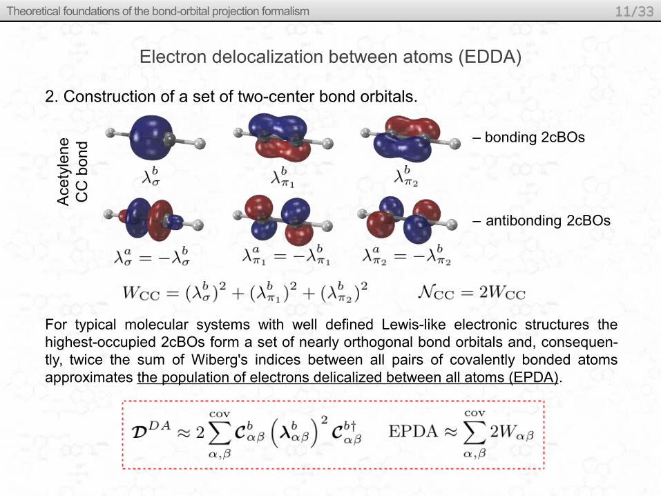
2. Construction of a set of two-center bond orbitals.
– the Jug's matrix is a (α,β)-diatomic block matrix of type: =
– for duodemponent density matrices, the Wiberg's bond-order (covalency) index reads:
– the eigenvectors of represent the two-center bond orbitals of three different types: bonding >0, non-bonding =0, and antibonding <0
, and both subsets of 2cBOs form a paired-orbital basis.
– electron density in the NAO basis reads
Theoretical foundations of the bond-orbital projection formalism 10/33
Electron delocalization between atoms (EDDA)
2. Construction of a set of two-center bond orbitals.
Ace
tyle
ne
CC
bo
nd
– bonding 2cBOs
– antibonding 2cBOs
For typical molecular systems with well defined Lewis-like electronic structures the highest-occupied 2cBOs form a set of nearly orthogonal bond orbitals and, consequen-tly, twice the sum of Wiberg's indices between all pairs of covalently bonded atoms approximates the population of electrons delicalized between all atoms (EPDA).
Theoretical foundations of the bond-orbital projection formalism 11/33

Electron delocalization between atoms (EDDA)
Obviously, for accurate calculations as well as in the case of large molecular systems with non-typical bonds and weak interactions, twice the sum of Wiberg's covalencies sometimes exceeds the exact EPDA due to nonorthogonal overcounting. In such situations we have two choices:
all = ( )n2
I. Restore orthogonality of the highest-occupied 2cBOs within the iterative double-atom partitioning procedure using orthogonal projectors or, more familiar, by transformation to the subset of bonding NBOs.
II. Remove the nonorthogonal electron overcounting by the following projection cascade:
NAO → MO(occupied) → 2cBO(bonding) → MO(occupied) → NAO ,
which is fully equivalent to the following orthogonal similarity transformation:
3. Projection of 2cBOs onto the subspace of occupied MOs
Theoretical foundations of the bond-orbital projection formalism 12/33

Electron delocalization between atoms (EDDA)
… a little too much! So where is the problem?
0
Num
ber
of π
-ele
ctro
ns
2
4
6
8
4.8
00
4.3
11
6.0
00
4.8
89
6.8
57
4.9
03
7.5
00
4.7
68
14%25%
Projections through the subspace of occupied MOs remove π-electron overcounting...
C5H
5- C
6H
6 C
7H
7+ C
8H
82+
3. Projection of 2cBOs onto the subspace of occupied MOs
Theoretical foundations of the bond-orbital projection formalism 13/33

Electron delocalization between atoms (EDDA)
Due to nonorthogonalities both bonding and antibonding 2cBOs are linear combinations of MOocc and MOvir. Therefore, the projection cascade MUST involve both 2cBO subspaces.
3. Projection of 2cBOs onto the subspace of occupied MOs
!
Theoretical foundations of the bond-orbital projection formalism 14/33
+
NAO → MO(occupied) → 2cBO(all) → MO(occupied) → NAO
c o m p l e m e n t a r y

Electron delocalization between atoms (EDDA)
0
Num
ber
of π
-ele
ctro
ns
2
4
6
814%
25%
C5H
5- C
6H
6 C
7H
7+ C
8H
82+
4.8
004
.311
5.7
60
6.0
00
4.8
89
6.0
00
6.8
57
4.9
03
5.8
77
7.5
00
4.7
68
5.6
25
3. Projection of 2cBOs onto the subspace of occupied MOs
Theoretical foundations of the bond-orbital projection formalism 15/33
NAO → MO(occupied) → 2cBO(all) → MO(occupied) → NAO
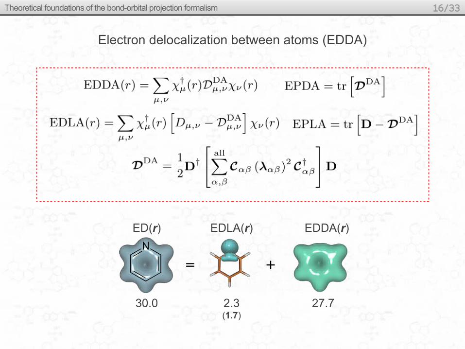
Electron delocalization between atoms (EDDA)
ED(r) EDLA(r) EDDA(r)
30.0 2.3(1.7)
27.7
Theoretical foundations of the bond-orbital projection formalism 16/33
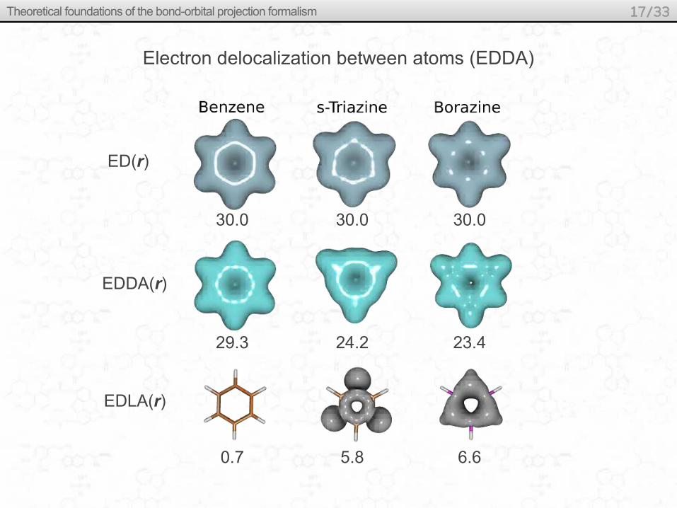
Electron delocalization between atoms (EDDA)
ED(r)
EDDA(r)
EDLA(r)
30.0 30.0 30.0
29.3 24.2 23.4
0.7 5.8 6.6
Theoretical foundations of the bond-orbital projection formalism 17/33

Electron delocalization between bonds
The EDDA component of the electron density can be further partitioned:
EDLB(r) EDDB(r)EDDA(r) = +
EDLB(r)
EDDB(r)
– electron density of localized (two-center) bonds,
– electron density of delocalized (multi-center) bonds,
EPLB
EPDB
0 – localized 2cBO
1 – delocalized 2cBO
Theoretical foundations of the bond-orbital projection formalism 18/33

Construction of the matrix
1. Forming two sets of 2cBOs for adjacent bonds Xα–X
β and X
β–X
γ, ie.
and , respectively.
2. Forming a set of three-center bond orbitals (3cBO), .
3. Expanding bonding 3cBOs in the basis of orthogonalized bonding 2cBOs.
4. Canceling of the phase-opposite 3cBOs.
5. Determining scaling factors .
6. Removing the nonorthogonal electron overcounting.
Electron delocalization between bonds
Theoretical foundations of the bond-orbital projection formalism 19/33
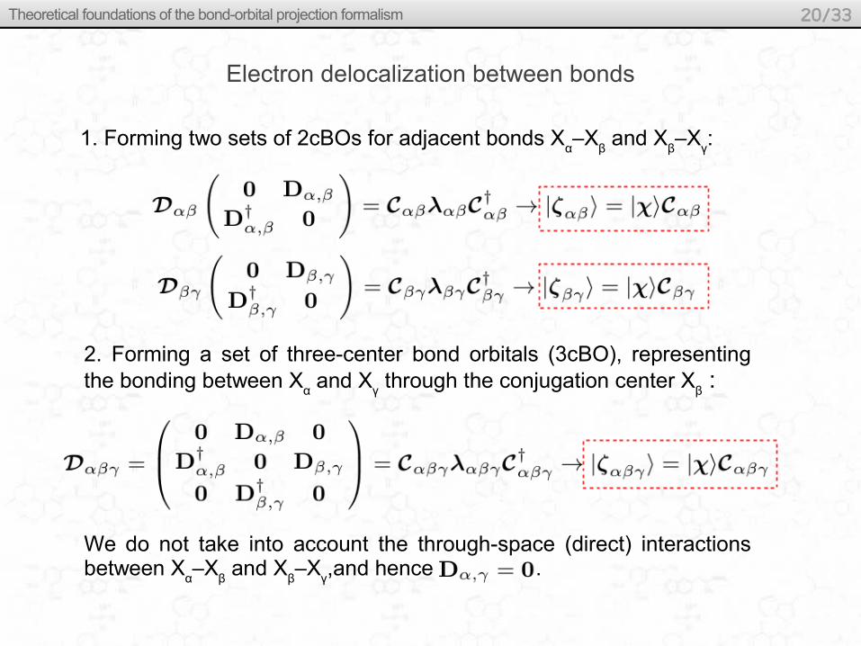
Electron delocalization between bonds
1. Forming two sets of 2cBOs for adjacent bonds Xα–X
β and X
β–X
γ:
2. Forming a set of three-center bond orbitals (3cBO), representing the bonding between X
α and X
γ through the conjugation center X
β :
We do not take into account the through-space (direct) interactions between X
α–X
β and X
β–X
γ,and hence .
Theoretical foundations of the bond-orbital projection formalism 20/33

Electron delocalization between bonds
3. Expanding bonding 3cBOs in the basis of orthogonalized bonding 2cBOs.
Orthogonalization: OW SO
= –
3cBO 2cBO 2cBO
Theoretical foundations of the bond-orbital projection formalism 21/33

Electron delocalization between bonds
4. Canceling out the phase-opposite 3cBOs.
If two linear combinations of 2cBOs are in opposite pha-ses and have nearly degenerated occupation numbers, they do not contribute to bond delocalization. Phase-opposite!If two 2cBOs do not form effectively a 3cBO they do not contribute to bond delocalization.! Effective
3cBO Effective2cBO
To determine if and to what extent both conditions are satisfied we can use an auxiliary vector with the elements defined as follows (we assume that 3cBOs are ordered from the highest to lowest occupied):
where ,
= 1 (effective 3cBO)
= –1 (effective 3cBO but in opposite phase with other 3cBO)
= 0 (effective 2cBO)
Theoretical foundations of the bond-orbital projection formalism 22/33
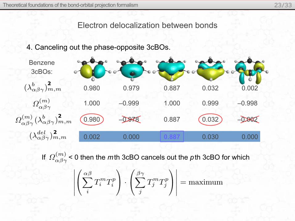
Electron delocalization between bonds
4. Canceling out the phase-opposite 3cBOs.
0.980 0.979 0.887 0.032 0.002
1.000 –0.999 1.000 0.999 –0.998
0.980 0.887 0.032 –0.002–0.978
0.002 0.000 0.887 0.030 0.000
Benzene3cBOs:
If < 0 then the m th 3cBO cancels out the p th 3cBO for which
2
2
2
Theoretical foundations of the bond-orbital projection formalism 23/33

Electron delocalization between bonds
5. Determining scaling factors .
To determine the scaling factor for the i th 2cBO of the Xα–X
β bond we have
to consider conjugations with 2cBOs of all possible adjacent bonds.
6. Removing the nonorthogonal electron overcounting.
Theoretical foundations of the bond-orbital projection formalism 24/33
*
order– reversed ,
assuming that:

Localization and delocalization components of the electron density
Theoretical foundations of the bond-orbital projection formalism 25/33

Localization and delocalization components of the electron density
Theoretical foundations of the bond-orbital projection formalism 26/33
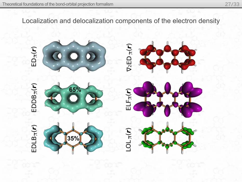
Localization and delocalization components of the electron density
65%
35%
Theoretical foundations of the bond-orbital projection formalism 27/33

The effectiveness of bond conjugation as an aromaticity criterion
GLOBAL/LOCAL AROMATICITYHÜCKEL's AROMATICITY
Theoretical foundations of the bond-orbital projection formalism 28/33
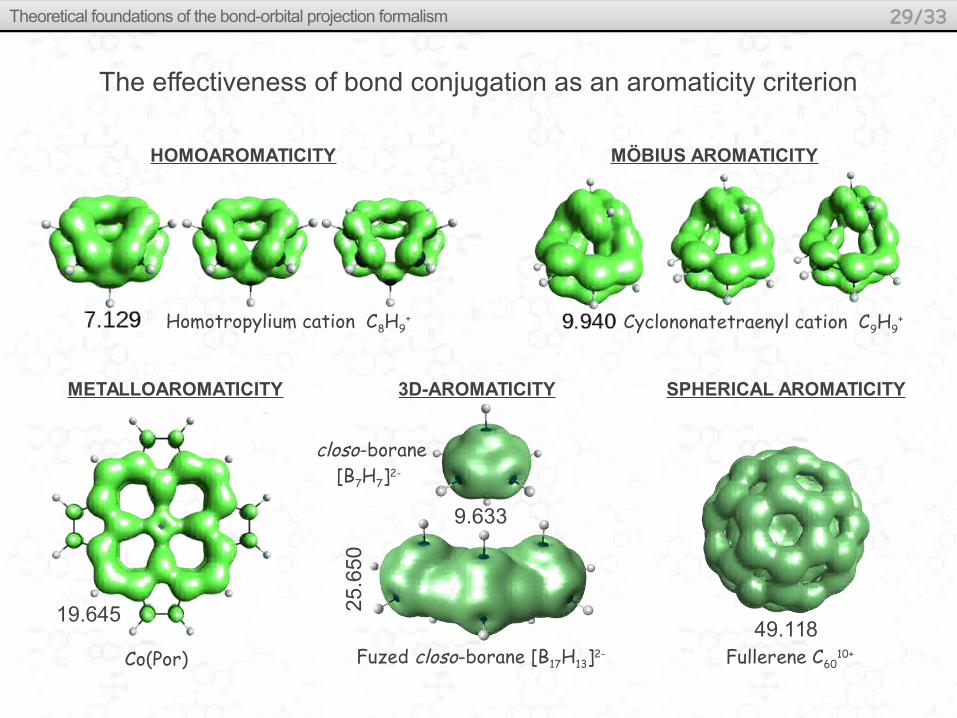
Homotropylium cation C8H9+
HOMOAROMATICITY
Cyclononatetraenyl cation C9H9+
MÖBIUS AROMATICITY
Fullerene C6010+
SPHERICAL AROMATICITY3D-AROMATICITY
closo-borane [B7H7]2-
Fuzed closo-borane [B17H13]2-
9.633
25.6
50
METALLOAROMATICITY
19.645
Co(Por)49.118
The effectiveness of bond conjugation as an aromaticity criterion
Theoretical foundations of the bond-orbital projection formalism 29/33

The effectiveness of bond conjugation as an aromaticity criterion
Theoretical foundations of the bond-orbital projection formalism 30/33
k
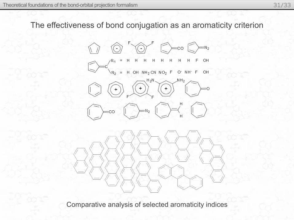
The effectiveness of bond conjugation as an aromaticity criterion
Comparative analysis of selected aromaticity indices
Theoretical foundations of the bond-orbital projection formalism 31/33

Comparative analysis of selected aromaticity indices
The effectiveness of bond conjugation as an aromaticity criterion
Theoretical foundations of the bond-orbital projection formalism 32/33
*
*By courtesy of dr Justyna Dominikowska
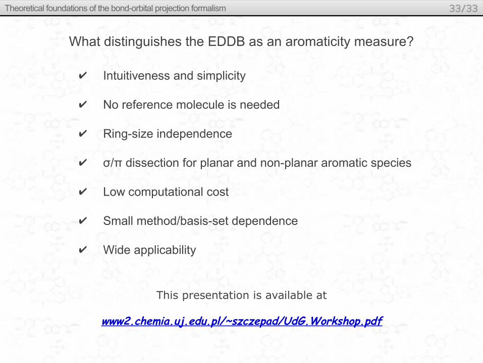
What distinguishes the EDDB as an aromaticity measure?
✔ Intuitiveness and simplicity
✔ No reference molecule is needed
✔ Ring-size independence
✔ σ/π dissection for planar and non-planar aromatic species
✔ Low computational cost
✔ Small method/basis-set dependence
✔ Wide applicability
Theoretical foundations of the bond-orbital projection formalism 33/33
This presentation is available at
www2.chemia.uj.edu.pl/~szczepad/UdG.Workshop.pdf

A new perspective on quantifying electron localization and delocalization in molecular systems
A practical guide to the use of the EDDB method
A new perspective on quantifying electron localization and delocalization in molecular systems
A practical guide to the use of the EDDB method
JAGIELLONIAN UNIVERSITYDepartment of Theoretical Chemistry
Institut de Química Computacional i Catàlisi
WORKSHOP
GIRONAJanuary 28st, 2016
dr Dariusz Szczepanik
Updated: 2016-02-25

A practical guide to the use of the EDDB method
1. Electron density of delocalized bonds.
2. Installation, configuration and execution of the RunEDDB program
3. Visualization of EDDB and related functions.
4. Selected examples:
2/40
Presentation plan
4.1. Relative aromaticity along different conjugation paths.
4.2. Multifold aromaticity in all-metal clusters.
4.3. Local and global aromaticity in polycyclic aromatic species.
5. Plans for future development.

Electron density of delocalized bonds
ED(r) EDLA(r) EDLB(r) EDDB(r)
ED(r)
EDLA(r)
EDLB(r)
EDDB(r)
– electron density,
– density of electrons localized on atoms,
– electron density of localized bonds,
– electron density of delocalized bonds.
..
A practical guide to the use of the EDDB method 3/40
arom
atic
stab
iliza
tion
!

A practical guide to the use of the EDDB method 4/40
Electron density of delocalized bonds
EPDB
– one-electron density matrix within the NAO basis
– off-diagonal (α,β)-diatomic block of
– two-center bond orbital (2cBO)
– diagonal matrix of the 2cBO occupations
– diagonal matrix of scaling factors for each 2cBO
(delocalized 2cBO)(localized 2cBO)
One
-det
erm
inan
tCl
osed
-she
ll
For
open
-she
ll sy
stem
s D
DB i
s de
fine
d as
twi
ce t
he s
um
of t
he c
orre
spon
ding
spi
n co
mpo
nent
s

A practical guide to the use of the EDDB method 5/40
✔ Intuitiveness and interpretational simplicity✔ No parametrization and reference molecule is needed✔ Ring-size independence✔ σ/π dissection for planar and non-planar aromatic species✔ Low computational cost ✔ Small method/basis-set dependence✔ Wide applicability
Electron density of delocalized bonds
What distinguishes the EDDB as an aromaticity measure?
References
(1) Electron delocalization index based on bond order orbitals D.W. Szczepanik, E. Żak, K. Dyduch, J. Mrozek, Chem. Phys. Lett. 593 (2014) 154-159.
(2) A uniform approach to the description of multicenter bonding D.W. Szczepanik, M. Andrzejak, K. Dyduch, E. Żak, M. Makowski, G. Mazur, J. Mrozek, Phys. Chem. Chem. Phys. 16 (2014) 20514-20523.
(3) A new perspective on quantifying electron localization and delocalization in molecular systems D.W. Szczepanik, Comput. Theor. Chem. 1080 (2016) 33-37.

The current version of the RunEDDB program is available for Linux systems as a script written in R, and as such it requires the R-package (www.r-project.org).An up to date version of the script can be downloaded from:
A practical guide to the use of the EDDB method 6/40
Installation, configuration and execution of the RunEDDB program
www2.chemia.uj.edu.pl/~szczepad/RunEDDB (program)
(manual)www2.chemia.uj.edu.pl/~szczepad/RunEDDBman.pdf
To generate the cube files, the original Gaussian (www.gaussian.com) cubegen utility is required as well as the dat2cube bash script available at:
www2.chemia.uj.edu.pl/~szczepad/dat2cube
The method is based on the the NAO representation, which is provided by the NBO software (http://nbo6.chem.wisc.edu). To generate the FILE.49 file (containing the AO→NAO and NAO→MO matrices), an input file to the RunEDDB program, the following NBO keywords have to be used:
$NBO SKIPBO AONAO=W49 NAOMO=W49 $END
If you already have the .chk file you can generate the .49 file using this script:
www2.chemia.uj.edu.pl/~szczepad/chk249

A practical guide to the use of the EDDB method 7/40
Installation, configuration and execution of the RunEDDB program
1. Download the RunEDDB script:
wget P $HOME www2.chemia.uj.edu.pl/~szczepad/RunEDDB
2. If necessary, edit the first line to provide correct path to the Rscript interpreter. E.g., if the R-package is installed in /aplic/R/3.0.0/ then copy and paste this command:
sed i "1s/.*/\#\!\/aplic\/R\/3.0.0\/bin\/Rscript/" $HOME/RunEDDB
3. Make the script executable:
chmod a+x $HOME/RunEDDB
4. Create an alias to the script in the .bashrc file:
echo "alias runeddb='$HOME/RunEDDB'" >> $HOME/.bashrc
5. Repeat steps 1, 3 and 4 for scripts dat2cube and chk249.
Configuration...

A practical guide to the use of the EDDB method 8/40
Installation, configuration and execution of the RunEDDB program
1. Open an interactive session, e.g. :
qlogin clear q compilar.q
2. Load the R module, e.g.:
module load R/R3.0.0_ICS11.1.072
3. To support the cube files load also the appropriate Gaussian module,e.g.:
module load g09d01_pgi10.1_NBO6
4. To get FILE.49 from the Gaussian checkpoint file run the chk249 script:
chk249 FILE.chk
Execution...
What is the general syntax of the command line options for RunEDDB?
4. To perform the EDDB analysis (e.g. benzene / RHF) simply run:
runeddb FILE.49 1:21
If the SGE queue system is used...

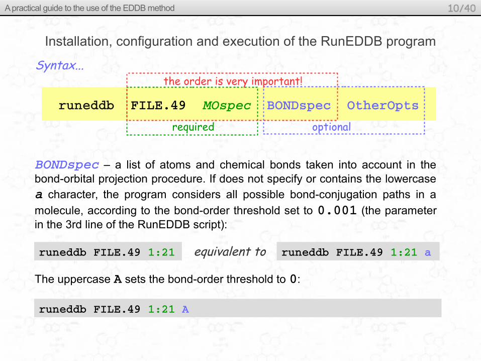
runeddb FILE.49 MOspec BONDspec OtherOpts
A practical guide to the use of the EDDB method 9/40
Installation, configuration and execution of the RunEDDB program
FILE.49 - file generated by the NBO module and containing the AO→NAO and NAO→MO transformation matrices.
required optional
MOspec – a list of occupied molecular orbitals, separated by commas; the range operator (:) is allowed (e.g. benzene / RHF, σ-MOs):
runeddb FILE.49 7:15,17,18,19
the order is very important!Syntax...
runeddb FILE.49 16,20:22 16,20
For UHF calculations MOspec lists have to be specified separately for alpha and beta molecular spinorbitals (e.g. benzene / UHF, π-MSOs):
runeddb FILE.49 MOspec BONDspec OtherOpts
A practical guide to the use of the EDDB method 10/40
Installation, configuration and execution of the RunEDDB program
BONDspec – a list of atoms and chemical bonds taken into account in the bond-orbital projection procedure. If does not specify or contains the lowercase a character, the program considers all possible bond-conjugation paths in a
molecule, according to the bond-order threshold set to 0.001 (the parameter in the 3rd line of the RunEDDB script):
required optional
runeddb FILE.49 1:21
the order is very important!Syntax...
The uppercase A sets the bond-order threshold to 0:
runeddb FILE.49 1:21 A
runeddb FILE.49 1:21 aequivalent to

runeddb FILE.49 MOspec BONDspec OtherOpts
A practical guide to the use of the EDDB method 11/40
Installation, configuration and execution of the RunEDDB program
Global aromaticity of naphthalene:(all possible bond conjugations)
required optional
the order is very important!Syntax… examples
BONDspec:
a
A
1:18
1:10,11,12,13:18
For medium/large species it is easier to specify atoms and fragments rather than bonds.
7.5e
runeddb FILE.49 MOspec BONDspec OtherOpts
A practical guide to the use of the EDDB method 12/40
Installation, configuration and execution of the RunEDDB program
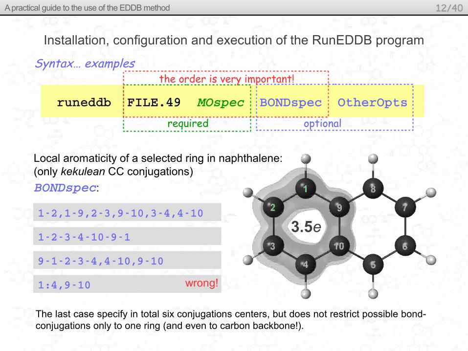
Local aromaticity of a selected ring in naphthalene:(only kekulean CC conjugations)
required optional
the order is very important!Syntax… examples
BONDspec:
12,19,23,910,34,410
12341091
91234,410,910
1:4,910
The last case specify in total six conjugations centers, but does not restrict possible bond-conjugations only to one ring (and even to carbon backbone!).
wrong!
3.5e

runeddb FILE.49 MOspec BONDspec OtherOpts
A practical guide to the use of the EDDB method 13/40
Installation, configuration and execution of the RunEDDB program
Local aromaticity of a selected ring in naphthalene:(kekulean + cross-ring CC conjugations)
required optional
the order is very important!Syntax… examples
BONDspec:
12341091,13,14,11 0,24,210,29,310,39,49
1:2:3:4:10:9
1,2,3,4,10,9 wrong!
4:1:9:2:3:10
The 3rd bond specification list is identical to the 2nd one. This notation allows one to restrict bond conjugations to particular molecular fragment only.
3.6e

A practical guide to the use of the EDDB method 14/40
runeddb FILE.49 MOspec BONDspec OtherOpts
Installation, configuration and execution of the RunEDDB program
required optional
the order is very important!Syntax…
OtherOpts:
EDED
EDLA
EDLB
EDDB
POFF – skip the orthogonal similarity transformation step.
– save the ED(r) function into the ED.dat file.
– save the EDLA(r) function into the EDLA.dat file.
– save the EDLB(r) function into the EDLB.dat file.
– save the EDDB(r) function into the EDDB.dat file.
NMB – restrict the EDDB analysis to the Natural Minimal Basis subspace only; it significantly reduces computational time.
These keywords can appear in the command line in any order.
In the case of spin-unrestric-ted open-shell calculations the corresponding spin-den-sities are saved into the SDXX.dat files in the same directory.

A practical guide to the use of the EDDB method 15/40
Installation, configuration and execution of the RunEDDB program
Results (benzene [singlet] / RHF) …
Atom ED EDLA EDLB EDDB 1 4.208 0.074 3.138 0.996 2 4.208 0.074 3.138 0.996 3 4.208 0.074 3.138 0.996 4 4.208 0.074 3.138 0.996 5 4.208 0.074 3.138 0.996 6 4.208 0.074 3.138 0.996 7 0.792 0.036 0.735 0.021 8 0.792 0.036 0.735 0.021 9 0.792 0.036 0.735 0.021 10 0.792 0.036 0.735 0.021 11 0.792 0.036 0.735 0.021 12 0.792 0.036 0.735 0.021 Total: 30.000 0.656 23.242 6.101 Computational cost: 00:00:01 (660x3cBO)
runeddb FILE.49 7:21 A
B3LYP/6-311+G(d,p)

A practical guide to the use of the EDDB method 16/40
Installation, configuration and execution of the RunEDDB program
Results (benzene [triplet] / UHF) …
Atom ED SD EDLA SDLA EDLB SDLB EDDB SDDB 1 4.264 0.178 0.232 0.014 3.390 0.074 0.642 0.091 2 4.169 0.605 0.306 0.184 3.331 0.203 0.533 0.219 3 4.169 0.605 0.306 0.184 3.331 0.203 0.533 0.218 4 4.264 0.178 0.232 0.014 3.390 0.074 0.642 0.091 5 4.169 0.605 0.306 0.184 3.331 0.203 0.533 0.218 6 4.169 0.605 0.306 0.184 3.331 0.203 0.533 0.218 7 0.789 0.004 0.036 0.001 0.731 0.005 0.021 0.000 8 0.804 0.018 0.032 0.005 0.758 0.022 0.015 0.001 9 0.804 0.018 0.032 0.005 0.758 0.022 0.015 0.001 10 0.789 0.004 0.036 0.001 0.731 0.005 0.021 0.000 11 0.804 0.018 0.032 0.005 0.758 0.022 0.015 0.001 12 0.804 0.018 0.032 0.005 0.758 0.022 0.015 0.001 Total: 30.000 2.000 1.887 0.725 24.596 0.586 3.518 0.689 Computational cost: 00:00:02 (1320x3cBO)
runeddb FILE.49 7:22 7:20 A
B3LYP/6-311+G(d,p)

A practical guide to the use of the EDDB method 17/40
dat2cube FILE.fchk EDXX.dat ngrid nproc
Visualization of EDDB and related functions
required optional
the order is very important!Syntax…
In the current implementation, the dat2cube script requires a formatted check-point file (FILE.fchk) from Gaussian and the EDXX.dat file obtained from the RunEDDB program. By default, dat2cube uses 1 CPU to generate a cube file with the number of points per side equal to 803=512k. It can be changed by specifying parameters nroc and ngrid, respectivety. E.g.
dat2cube FILE.fchk EDDB.dat 100 4
uses 4 CPUs to convert EDDB.dat into the cube file, EDDB.cube, containing 1003 points distributed evenly over a rectangular grid.
Which programs support the Gaussian cube format?
GaussView, (g)Molden, Molekel, VMD, Gabedit, Avogadro, ...

A practical guide to the use of the EDDB method 18/40
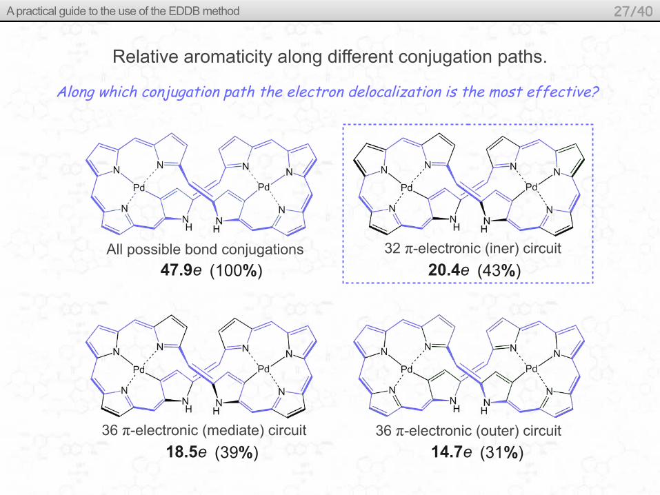
Relative aromaticity along different conjugation paths.
Bis-palladium(II) [36]octaphyrin(1.1.1.1.1.1.1.1)?
wget www2.chemia.uj.edu.pl/~szczepad/octaphyrin.tar.gz
tar xzf octaphyrin.tar.gz
qlogin clear q compilar.q
module load R/R3.0.0_ICS11.1.072
module load g09d01_pgi10.1_NBO6
B3LYP/SDD
Along which conjugation path the electron delocalization is the most effective?

A practical guide to the use of the EDDB method 19/40
Relative aromaticity along different conjugation paths.
All possible bond conjugations
runeddb FILE.49 1:178 a eddb > EDDB.all.log
dat2cube molecule.fchk EDDB.all.dat 80 1
mv EDDB.dat EDDB.all.dat

A practical guide to the use of the EDDB method 20/40
Relative aromaticity along different conjugation paths.
The conjugated 32 π-electronic (iner) circuit
runeddb FILE.49 1:178 126549101215181926242829363437384342414647495355566361656668691 eddb > EDDB.in.log
dat2cube molecule.fchk EDDB.in.dat 80 1
mv EDDB.dat EDDB.in.dat
1
2 65
49 10
1215
18
19
26
2428
2936
3437
384342
414647
4953
55
56
63
6165 66
68 69

A practical guide to the use of the EDDB method 21/40
Relative aromaticity along different conjugation paths.
The conjugated 36 π-electronic (mediate) circuit
1
2 65
410
1215
18
19
21
242829
36
3437
384342
414647
4953
55
56
58
61 65 6668 69
runeddb FILE.49 1:178 1265491012151819212224282936343738434241464749535556585961656668691 eddb > EDDB.med.log
dat2cube molecule.fchk EDDB.med.dat 80 1
mv EDDB.dat EDDB.med.dat
2259

A practical guide to the use of the EDDB method 22/40
Relative aromaticity along different conjugation paths.
The conjugated 36 π-electronic (outer) circuit
1
23
410 13
15
18
19
21
24282931
3437
3840
41464750
53
55
56
58
61 6566 71
692259
runeddb FILE.49 1:178 123491013141518192122242829313234373840414647505153555658596165667170691 eddb > EDDB.out.log
dat2cube molecule.fchk EDDB.out.dat 80 1
mv EDDB.dat EDDB.out.dat
9 14
32
51
70

A practical guide to the use of the EDDB method 23/40
Relative aromaticity along different conjugation paths.
All possible bond conjugations
Atom ED EDLA EDLB EDDB
Total: 356.000 140.207 167.939
Computational cost: 00:00:37 (23022x3cBO)
...
...
...
...
...
47.854
EDDB.all.log
EDDB.all.cube
without threshold: 00:07:45 (194472x3cBO)
48.389

A practical guide to the use of the EDDB method 24/40
Relative aromaticity along different conjugation paths.
The conjugated 32 π-electronic (iner) circuit
Atom ED EDLA EDLB EDDB
Total: 356.000 NA 68.771
Computational cost: 00:00:01 (34x3cBO)
...
...
...
...
...
20.419 (43%)
EDDB.in.log
EDDB.in.cube

A practical guide to the use of the EDDB method 25/40
Relative aromaticity along different conjugation paths.
The conjugated 36 π-electronic (mediate) circuit
Atom ED EDLA EDLB EDDB
Total: 356.000 NA 76.380
Computational cost: 00:00:01 (36x3cBO)
...
...
...
...
...
18.510 (39%)
EDDB.med.log
EDDB.med.cube

A practical guide to the use of the EDDB method 26/40
Relative aromaticity along different conjugation paths.
The conjugated 36 π-electronic (outer) circuit
Atom ED EDLA EDLB EDDB
Total: 356.000 NA 85.511
Computational cost: 00:00:01 (38x3cBO)
...
...
...
...
...
14.674 (31%)
EDDB.out.log
EDDB.out.cube
A practical guide to the use of the EDDB method 27/40
Relative aromaticity along different conjugation paths.
36 π-electronic (mediate) circuit
32 π-electronic (iner) circuit
36 π-electronic (outer) circuit
All possible bond conjugations
47.9e (100%) 20.4e (43%)
18.5e (39%) 14.7e (31%)
Along which conjugation path the electron delocalization is the most effective?

A practical guide to the use of the EDDB method 28/40
wget www2.chemia.uj.edu.pl/~szczepad/allmetaroma.tar.gz
qlogin clear q compilar.q
tar xzf allmetaroma.tar.gz
module load R/R3.0.0_ICS11.1.072
module load g09d01_pgi10.1_NBO6
B3LYP/X/Stuttgart+2f
Single,doubleortriplearomaticity?
Multifold aromaticity in all-metal clusters.
B3LYP/6-311+G(d)
Al
AlAl
Al
2-
Cu Cu
Cu
+
Y Y
Y
-
Hf Hf
Hf

A practical guide to the use of the EDDB method 29/40
runeddb Al42.49 21:27 A > Al42.all.log
Multifold aromaticity in all-metal clusters.
2-
21 22 23 24 25
runeddb Al42.49 21:26 A > Al42.sigma.log
runeddb Al42.49 27 A > Al42.pi.log
Al
AlAl
Al
26 27
A practical guide to the use of the EDDB method 30/40
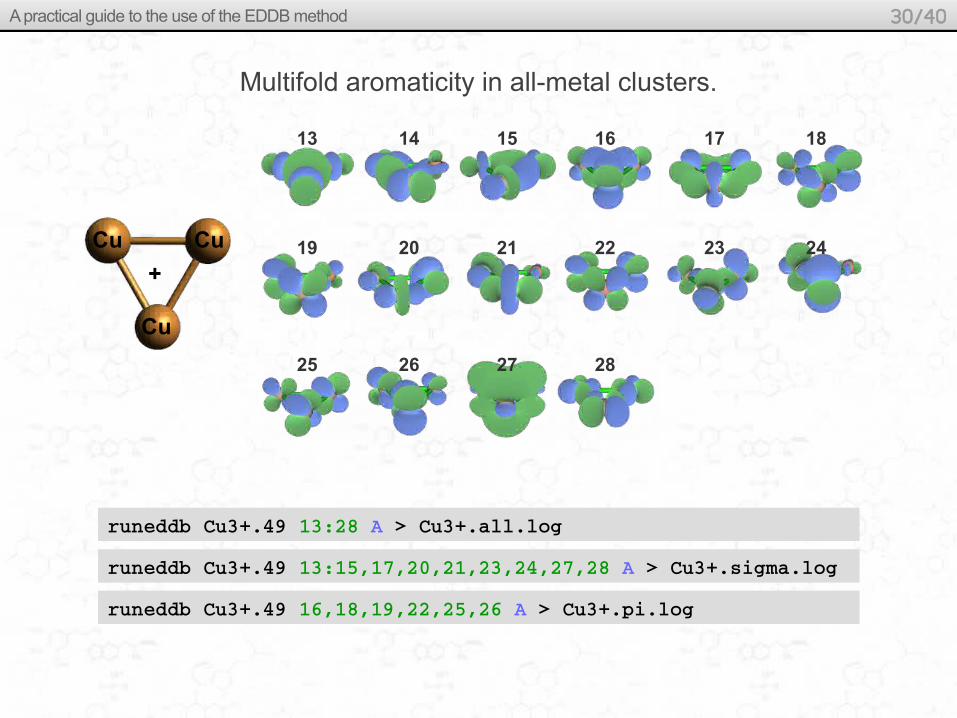
runeddb Cu3+.49 13:28 A > Cu3+.all.log
Multifold aromaticity in all-metal clusters.
Cu Cu
Cu
+
13 14 15 16 17 18
19 20 21 22 23 24
25 26 27 28
runeddb Cu3+.49 13:15,17,20,21,23,24,27,28 A > Cu3+.sigma.log
runeddb Cu3+.49 16,18,19,22,25,26 A > Cu3+.pi.log

A practical guide to the use of the EDDB method 31/40
runeddb Y3.49 13:17 A > Y3.all.log
Multifold aromaticity in all-metal clusters.
13 14 15 16 17
runeddb Y3.49 13:16 A > Y3.sigma.log
runeddb Y3.49 17 A > Y3.pi.log
Y
Y
Y -
runeddb Hf3.49 13:18 A > Hf3.all.log
13 14 15 16 17
runeddb Hf3.49 13:16 A > Hf3.sigma.log
runeddb Hf3.49 17 A > Hf3.pi.log
Hf Hf
Hf
18
runeddb Hf3.49 18 A > Hf3.delta.log
A practical guide to the use of the EDDB method 32/40
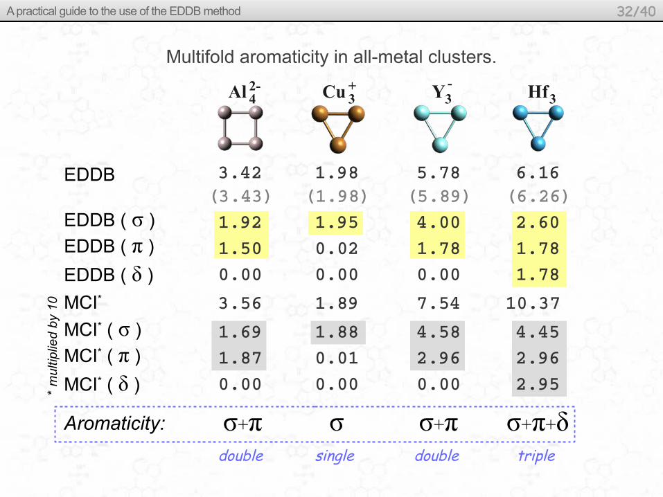
Multifold aromaticity in all-metal clusters.
Al Hf42- Cu 3
+ Y -3 3
EDDB ( σ )
EDDB ( π )
EDDB
EDDB ( δ )
3.42 (3.43) 1.92
1.50 0.00
MCI* ( σ )
MCI* ( π )
MCI* ( δ )
1.69 1.87
0.00
MCI* 3.56
Aromaticity:
1.98 (1.98) 1.95
0.02 0.00
1.88 0.01
0.00
1.89
5.78 (5.89) 4.00
1.78 0.00
4.58 2.96
0.00
7.54
6.16 (6.26) 2.60
1.78 1.78
4.45 2.96
2.95
10.37
σ+π σ σ+π σ+π+δdouble single double triple
* m
ultip
lied
by 1
0

A practical guide to the use of the EDDB method 33/40
Global and local π-aromaticity in polycyclic aromatic species.
wget www2.chemia.uj.edu.pl/~szczepad/glolocaroma.tar.gz
qlogin clear q compilar.q
tar xzf glolocaroma.tar.gz
module load R/R3.0.0_ICS11.1.072
module load g09d01_pgi10.1_NBO6
Does (and to what extent) the orthogonal similarity transformation affects local aromaticity?
B3LYP/6-311+G(d,p)
What is the influence of non-local conjugation effects on local aromaticity?

A practical guide to the use of the EDDB method 34/40
runeddb C6H6.49 17,20,21 1:2:3:4:5:6 > C6H6.global.log
Global and local π-aromaticity in polycyclic aromatic species.
runeddb C10H8.49 27,30,32:34 5:6:1:2:7:8:9:10:4:3 > C10H8.global.log
1 2
345
6
12
34
56
789
10 runeddb C10H8.49 27,30,32:34 1:2:3:4:5:6 > C10H8.local.log
Ben
zene
Nap
htha
lene

A practical guide to the use of the EDDB method 35/40
Global and local π-aromaticity in polycyclic aromatic species.
runeddb C16H10.49 39,43,46,49:53 1:2:3:4:5:6:11:12:13:14:15:16:17:18:22:23 > C16H10.global.log
1211
12
6
3 4 515
14
22 23
181716
runeddb C16H10.49 39,43,46,49:53 1:2:3:4:5:6 > C16H10.local.A.log
A
B
C
D13
runeddb C16H10.49 39,43,46,49:53 12:13:14:15:22:23 > C16H10.local.B.log
runeddb C16H10.49 39,43,46,49:53 11:12:13:14:15:16:17:18:22:23 > C16H10.local.C.log
runeddb C16H10.49 39,43,46,49:53 2:3:11:12:13 > C16H10.local.D.log
Flu
oran
then
e

A practical guide to the use of the EDDB method 36/40
Global and local π-aromaticity in polycyclic aromatic species.
6.501
3.211
3.211
5.327
11.828
3.139
0.9104.828
6.414
12.387 (+5%)
(-1%)
(-9%)
(-2%)
3.139(-2%)
Numbers inside rings stand for the (total) local EDDB populations. The outermost numbers are the (total) global EDDB populations Percentages in brackets refer to the effect of linking of benzene ring to naphthalene.
-40% compared to benzene

A practical guide to the use of the EDDB method 37/40
Global and local π-aromaticity in polycyclic aromatic species.
3.994
5.327
4.290
4.004 5.367
7.018 (+10%)
(+11%)
(+37%)
Numbers inside rings indicate the sum of the corresponding atomic contri-butions to the global EDDB population. Percentages in brackets show the effect of non-local conjugations on local aromaticity of particular ring..
4.290(+37%)
(+24%)
3.994(+24%)
(0%) +340%
The non-local conjugation effects are especially important in the cases of fused aromatic rings. But the the global EDDB populations should be used with a special caution due to overlap overcounting.
A practical guide to the use of the EDDB method 38/40
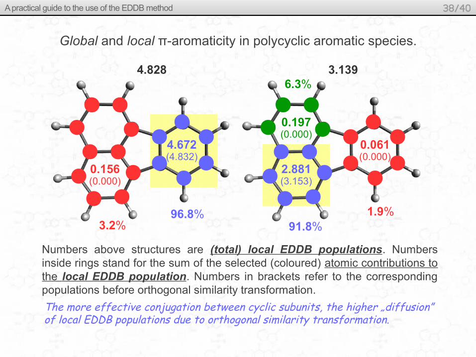
Global and local π-aromaticity in polycyclic aromatic species.
Numbers above structures are (total) local EDDB populations. Numbers inside rings stand for the sum of the selected (coloured) atomic contributions to the local EDDB population. Numbers in brackets refer to the corresponding populations before orthogonal similarity transformation.
4.672(4.832)
0.156(0.000)
96.8%3.2%
0.061(0.000)
0.197(0.000)
91.8%
6.3%
1.9%
2.881(3.153)
The more effective conjugation between cyclic subunits, the higher „diffusion” of local EDDB populations due to orthogonal similarity transformation.
4.828 3.139
A practical guide to the use of the EDDB method
Method
39/40
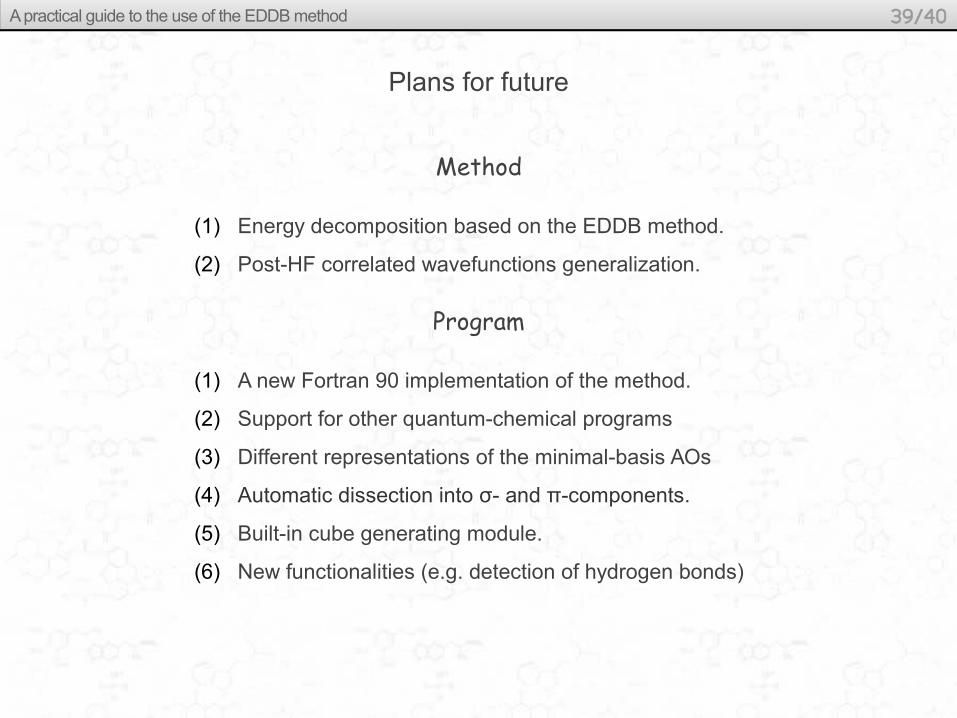
Plans for future
(1) Energy decomposition based on the EDDB method.
(2) Post-HF correlated wavefunctions generalization.
Program
(1) A new Fortran 90 implementation of the method.
(2) Support for other quantum-chemical programs
(3) Different representations of the minimal-basis AOs
(4) Automatic dissection into σ- and π-components.
(5) Built-in cube generating module.
(6) New functionalities (e.g. detection of hydrogen bonds)

A practical guide to the use of the EDDB method 40/40
A complete presentation of the EDDB method is available at
www2.chemia.uj.edu.pl/~szczepad/UdG.Workshop.pdf