Guided image filtering using signal subspace projection

Published in IET Image ProcessingReceived on 26th June 2012Revised on 31st October 2012Accepted on 20th November 2012doi: 10.1049/iet-ipr.2012.0351

ISSN 1751-9659

Guided image filtering using signal subspaceprojectionYong-Qin Zhang1,2, Yu Ding2, Jiaying Liu1, Zongming Guo1

1Institute of Computer Science and Technology, Peking University, Beijing 100871, People’s Republic of China2Paul C. Lauterbur Research Centre for Biomedical Imaging, Shenzhen Key Laboratory for MRI, Shenzhen Institutes

of Advanced Technology, Chinese Academy of Sciences, Shenzhen 518055, People’s Republic of China

E-mail: [email protected]

Abstract: There are various image filtering approaches in computer vision and image processing that are effective for some typesof noise, but they invariably make certain assumptions about the properties of the signal and/or noise which lack the generality fordiverse image noise reduction. This study describes a novel generalised guided image filtering method with the reference imagegenerated by signal subspace projection (SSP) technique. It adopts refined parallel analysis with Monte Carlo simulations to selectthe dimensionality of signal subspace in the patch-based noisy images. The noiseless image is reconstructed from the noisy imageprojected onto the significant eigenimages by component analysis. Training/test image are utilised to determine the relationshipbetween the optimal parameter value and noise deviation that maximises the output peak signal-to-noise ratio (PSNR). Theoptimal parameters of the proposed algorithm can be automatically selected using noise deviation estimation based on thesmallest singular value of the patch-based image by singular value decomposition (SVD). Finally, we present a quantitativeand qualitative comparison of the proposed algorithm with the traditional guided filter and other state-of-the-art methods withrespect to the choice of the image patch and neighbourhood window sizes.

www.ietdl.org

1 Introduction

Image denoising is still a challenging task in the procedures ofimage and video processing systems, for example acquisition,processing, coding, storage, transmission, reproduction andprinting. Whereas preserving image features such as edges,textures, and details, it refers to the recovery of a digitalimage that has been contaminated by some types of noise,for example Gaussian noise (AWGN), Rician noise, saltand pepper noise, speckle noise, impulse or Poisson noise.As far as we know, image denoising was first studied byNahi [1] and Lev et al. [2] in 1970s. Then in 1980s, Lee[3] introduced local statistics to study image enhancementand noise filtering. Donoho [4] and Simoncelli and Adelson[5] studied noise removal with wavelet transforms in late1990s. Subsequently many wavelet-based image denoisingalgorithms have appeared in these literatures [6–11].However, these methods often blur fine details and smoothout the edges.Since the non-local mean (NLM) algorithm by Buades

et al. [12] has renewed the interest into this classical inverseproblem, many more powerful denoising techniques havebeen proposed in the past several years [13–29]. However,the vast majority of image denoising algorithms haveimplicit assumptions on signal or attenuation properties,which limits the generality. The NLM algorithm [12] isbased on the image spatial self-similarity with betterperformance than traditional denoising methods, but itssimilarity measurement between the target pixel and its

270& The Institution of Engineering and Technology 2013

associated pixels is related to noise types. The discreteuniversal denoising (DUDE) method proposed byWeissman et al. [14] uses the similarity of the statisticalregion for text correction, character recognition, and imagedenoising and achieves good performance, whereas DUDEis less effective to eliminate the additive noise. In addition,it depends on the statistical probability of the pixel’sneighbourhood and the signal is limited to discrete values.The unsupervised, information-theoretic, adaptive imagefiltering (UINTA) in [15] adopted Markov nature of theinput image from different contexts to learn the conditionalprobability density function (PDF) and update the pixelvalues in order to reduce the randomness. However, UINTAemploys information entropy as decision criterion that alsodamages the details and textures of the image. TheTLS-based algorithm proposed by Hirakawa and Parks in[18], needs accurate estimation of noise parameters. Thekernel regression (KR) method with recursive iterationsproposed by Takeda et al. [22] has expensive computation,and is difficult to achieve real-time processing. Thedenoising algorithm using grey polynomial proposed byZhang et al. [23] can acquire better filtering effect of saltand pepper noise, but has poor results for additive Gaussiannoise. The guided filter approach [24] can remove imagenoise and preserve edges. However, it has poorperformance in the low SNR images. It also lacks ofreliable approach to optimally select parameters, whichseriously affects its practicality. The bilateral filter [21, 25]compares only intensity level values in a single pixel,

IET Image Process., 2013, Vol. 7, Iss. 3, pp. 270–279doi: 10.1049/iet-ipr.2012.0351

www.ietdl.org
which is not robust when these values are corrupted by highlevel noise. Nevertheless, if the assumptions contained in thedenoising techniques cannot be met, such filters will lead toblurred edges and loss of fine structures.As we know, for a single input noisy image, it is also
used as the reference image of guided image filteringmethod for weight calculation [24, 30]. Inspired by both theKarhunen–Loeve transform (KLT) filter [26] and jointbilateral filter approach [31], we develop a novel algorithmbased on local linear minimum mean-square error(LMMSE) predictors to achieve resolution enhancement fornoisy images and to improve the preservation of edgesharpness. Comparing to the existing guided filteringtechnique [24, 30], the proposed method utilises theprojection of the patch-based image onto signal subspacedetermined by improved parallel analysis with Monte Carlosimulation as the reference image. The smallest singularvalue of the patch-based image matrix is the estimate of thenoise standard deviation, and the regularisation parametersare automatically selected by polynomial fitting technique.A comparison of the proposed approach with the state ofthe arts is also presented.The rest of this paper is organised as follows. In Section 2,

we briefly review the related concepts, and the proposedscheme of single image denoising is described here. Section3 shows the simulation and experimental results of theproposed algorithm, and the comparison to the state-of-the-arts methods. Finally, we discuss the key findings andconclude our study in Section 4.

2 Proposed algorithm

In real-world digital-imaging devices, the acquired images areoften corrupted by device specific noise. Mathematically, thegoal of image denoising methods is to recover the clean imagefrom an observed noisy measurement. And the mixed noisemodel of independent additive and multiplicative types isgenerally used to describe the noisy image [18]

x = s+ n0 + n1s (1)

where x is the observed image, s is the ideal noiseless image,and n0 and n1 represent additive and multiplicative noises,respectively. Many literatures prefer working with anindependent additive noise [12, 15, 22], such as Gaussiannoise model. That is to say, a simplified noise modelinstead of (1) denoting the degradation process, is given inthe following formula

x = s+ n0 (2)

Where x and s are defined in (1). Note that (2) is a special caseof (1). Although the mathematical elegance and simplicitymakes (2) attractive for the complex task of designing adenoising algorithm and describing a natural image, thisnoise model often requires additional techniques to describethe real-world systems. The image denoising algorithmattempts to obtain the best estimate of s from x. Theoptimisation criterion can be mean-squared error(MSE)-based or perceptual quality driven, whereas theproblem of image quality assessment has not been resolved,especially in the absence of an original reference.


2.1 Formulation of stacked patches

The scene captured in data acquisition or data storage is oftena single image or multiple images deteriorated by variousnoise sources. Consequently, the image denoising hasbecome a key focus of ongoing studies in recent years.Assume that xi denotes the ith pixel in the observed imageX∈RM ×N and Y is a column stacked patch-basedrepresentation of X, that is, Y is a matrix of size L × Pwhere L =M ×N, whose each row contains the

��P

√ × ��P

√patch around the location of xi in the image X. Moreover,image patch centred at a pixel on the matrix border ispadded with mirror copies of the array elements.

2.2 Matrix decomposition of patch-based image

The singular value decomposition (SVD) operator, whichtransfers a set of correlated variables into a new set ofuncorrelated variables, has the interesting properties thatthey capture the variation of functions defined on the graphfrom the largest to the smallest singular values. Theseeigenfunctions form the basis for a real or complex matrix.We find that most of the energy of a function defined onthe graph is concentrated at several principal components.Moreover, the eigenfunctions generated from noisy data areable to capture the main characteristics of the correspondingclean signal, whereas the eigenvectors of the smallersingular values are almost all noise.By removing the mean value from each row, the difference

vectorised image from the patch-based image matrix iscomputed as

Z(i, p) = Y (i, p)− 1

L

∑Li=1

Y (i, p) (3)

where i = 1, 2,…, L, and p = 1, 2,…, P.To reduce computation time, the covariance matrix ZTZ

instead of Z is used to be factorised by this form

ZTZ = US2UT (4)

where the symbol T denotes the transpose operator, and U isthe unitary matrix of eigenvectors derived from ZTZ. Σ is aP × P diagonal matrix with its singular values λ1 ≥ λ2≥…≥ λr≥ 0 and r = rank (ZTZ).After the projection of Z onto the new basis U, the

reformed uncorrelated matrix Z is

Z = Z× U (5)

Therefore the new axes are the eigenvectors of the correlationmatrix of the original variables, which capture the similaritiesof the original variables based on how data samples projectedonto them. As we know, if the eigenvalues are very small andthe size of image patch from a single noisy image is largeenough, the removing eigenmodes of the less significancedo not lose much information. From the diagonal singularvalues, only the first K eigenvectors are chosen based ontheir eigenvalues. Since the parameter K should be not onlylarge enough enough to allow fitting the characteristics ofthe data, but also small enough to filter out the non-relevantnoise and redundancy. Therefore, the top K largest valuesare properly selected by PA with Monte Carlo simulation.


www.ietdl.org
2.3 Proposed number of factors to retain
The PA firstly introduced by Horn [32, 33], which in fact is aMonte Carlo simulation technique, compares the observedeigenvalues extracted from the correlation matrix to beanalysed with those of an artificial data set obtained fromuncorrelated normal variables. This data set is generated bydrawing samples from a multivariate normal distributionwith the dimensionality P, the same number of observationsL, and the same marginal standard deviations as the actualdata. Let λp for 1≤ p≤ P denote the singular values of thevectorised patch-based image Z sorted in descending order.Similarly, let αp denote the descendingly sorted singularvalues of the artificial data matrix. Therefore PA estimatesdata dimensionality as

K = max 1 ≤ p ≤ P|lp ≥ ap

{ }( )(6)

The intuition is that αp is a threshold for λp below which thep’th component is judged to have occurred because of chance.Currently, it is recommended to use the singular value of theartificial data that corresponds to a given percentile, such asthe 95th of the distribution of singular values derived fromthe random data.In our algorithm, without the assumption of a given

random distribution, we generate the artificial data byrandomly permuting each element of the neighbourhoodvector centered at each pixel. Let yi, p denote the p’thelement of the patch-based neighbourhood vector yi, centredat pixel position xi. For each P elements of the vector yi, arandom permutation of the index sequence p = 1, 2,…, P isgenerated by uniform distribution. Thus the mean value,maximum, minimum and random distribution of theartificial data is satisfied for each image patch-based vector.


Then the singular values α of the random artificial data arecomputed by SVDs which keeps the marginal distributionsintact whereas breaking any interdependencies betweenthem. For the L by P synthetic matrix C, after multipletimes (e.g. 50) of Monte Carlo simulations, summarystatistics (e.g. 95th percentile) can be used to extract the Psingular values and order them from largest to smallest.Then PA is applied and the intersection of the two linesdenoting singular values of the simulated data C anddifference vectorised image Z is the cutoff for determiningthe number of signal subspace dimensions present in thenoisy image. As we know, the noise variance is intimatelyrelated with the smallest singular value of simulated data[34]. From the theory and simulation, we found that thesingular values of noise matrix are different, whichapproximately linearly decrease gradually with thedimension. Therefore the increment between the smallestsingular value and the largest one from the simulated noisematrix can be used for dimensionality reduction of thenoisy image data. The our proposed approach of thecorrected singular values of the artificial data was given inthis formula

a(p) = b(p)− b(P)+ l(P)+ t(b(1)− b(P)) (7)

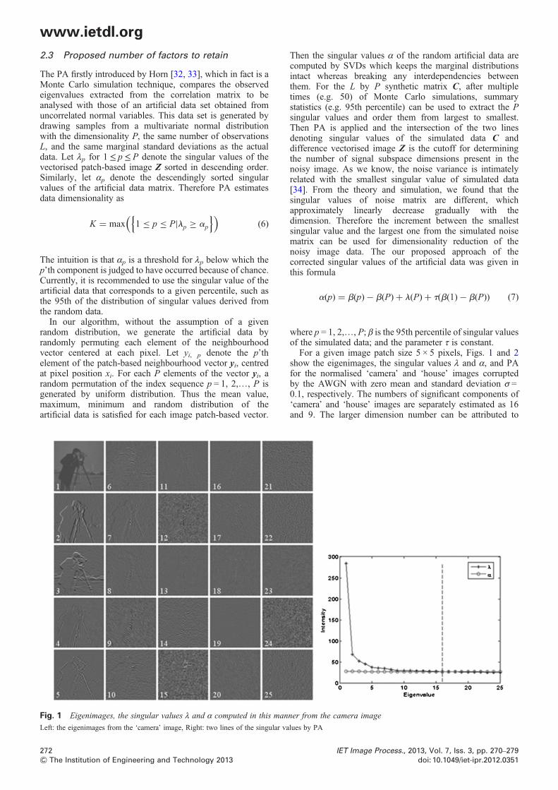
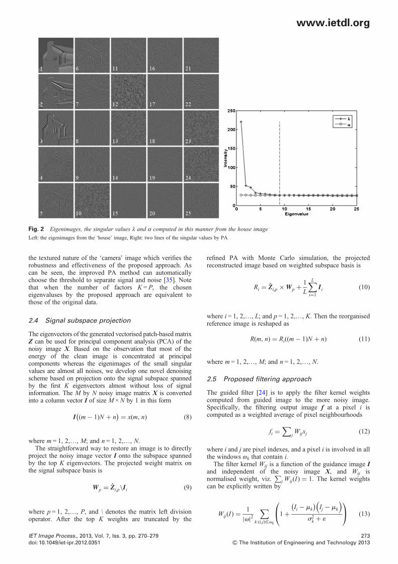
where p = 1, 2,…, P; β is the 95th percentile of singular valuesof the simulated data; and the parameter τ is constant.For a given image patch size 5 × 5 pixels, Figs. 1 and 2

show the eigenimages, the singular values λ and α, and PAfor the normalised ‘camera’ and ‘house’ images corruptedby the AWGN with zero mean and standard deviation σ =0.1, respectively. The numbers of significant components of‘camera’ and ‘house’ images are separately estimated as 16and 9. The larger dimension number can be attributed to

Fig. 1 Eigenimages, the singular values λ and α computed in this manner from the camera image

Left: the eigenimages from the ‘camera’ image, Right: two lines of the singular values by PA


www.ietdl.org

Fig. 2 Eigenimages, the singular values λ and α computed in this manner from the house image

Left: the eigenimages from the ‘house’ image, Right: two lines of the singular values by PA

the textured nature of the ‘camera’ image which verifies therobustness and effectiveness of the proposed approach. Ascan be seen, the improved PA method can automaticallychoose the threshold to separate signal and noise [35]. Notethat when the number of factors K = P, the choseneigenvaluses by the proposed approach are equivalent tothose of the original data.

2.4 Signal subspace projection

The eigenvectors of the generated vectorised patch-based matrixZ can be used for principal component analysis (PCA) of thenoisy image X. Based on the observation that most of theenergy of the clean image is concentrated at principalcomponents whereas the eigenimages of the small singularvalues are almost all noises, we develop one novel denoisingscheme based on projection onto the signal subspace spannedby the first K eigenvectors almost without loss of signalinformation. The M by N noisy image matrix X is convertedinto a column vector I of size M ×N by 1 in this form

I (m− 1)N + n( ) = x(m, n) (8)

where m = 1, 2,…, M; and n = 1, 2,…, N.The straightforward way to restore an image is to directly

project the noisy image vector I onto the subspace spannedby the top K eigenvectors. The projected weight matrix onthe signal subspace basis is

Wp = Zi,p\Ii (9)

where p = 1, 2,…, P, and \ denotes the matrix left divisionoperator. After the top K weights are truncated by the


refined PA with Monte Carlo simulation, the projectedreconstructed image based on weighted subspace basis is

Ri = Zi,p ×Wp +1

L

∑Li=1

Ii (10)

where i = 1, 2,…, L; and p = 1, 2,…, K. Then the reorganisedreference image is reshaped as

R(m, n) = Ri((m− 1)N + n) (11)

where m = 1, 2,…, M; and n = 1, 2,…, N.

2.5 Proposed filtering approach

The guided filter [24] is to apply the filter kernel weightscomputed from guided image to the more noisy image.Specifically, the filtering output image f at a pixel i iscomputed as a weighted average of pixel neighbourhoods

fi =∑

jWijxj (12)

where i and j are pixel indexes, and a pixel i is involved in allthe windows ωk that contain i.The filter kernel Wij is a function of the guidance image I

and independent of the noisy image X, and Wij isnormalised weight, viz.

∑j Wij(I ) = 1. The kernel weights

can be explicitly written by

Wij(I ) =1

|v|2∑

k:(i,j)[vk

1+Ii − mk

( )Ij − mk

( )

s2k + 1

⎛⎝

⎞⎠ (13)


www.ietdl.org
where |ω| is the total number of pixels in a window ωk; μk ands2k are the mean and variance in a window ωk of the guide
image I; and ε is a regularisation parameter.In previous literatures [24, 30], the guided image I and

input noisy image X are identical when the guided filter isused for single image denoising. However, the noiseexisting in guided image brings about distortion of therestored image, and also the parameter ε seriously affectsthe filtering results. To solve this problem, in the proposedalgorithm, we select the reconstructed reference image Reven though it still has some residual noise after signalsubspace projection (SSP) as the guided image I, andsimultaneously optimise the parameter ε under differentwindow size by noise deviation estimation for noisereduction further.For a given noisy image and a window ωk of pixel

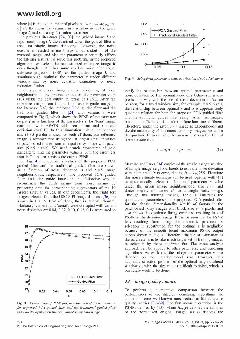
neighbourhood, the optimal choice of the parameter ε in(13) yields the best output in terms of PSNR. After thereference image from (11) is taken as the guide image inthe literature [24], the improved PCA guided filter and thetraditional guided filter in [24] with various ε werecompared in Fig. 3, which shows the PSNR of the estimatoroutput f as a function of the parameter ε for ‘lena’ imagecorrupted with AWGN with zero mean and standarddeviation σ = 0.10. In this simulation, while the windowsize (5 × 5 pixels) is used for both of them, our referenceimage is reconstructed using the 10 largest singular valuesof patch-based image from an input noisy image with patchsize (9 × 9 pixels). We used search procedures of goldstandard to find the parameter value ε with the error lessthan 10− 6 that maximises the output PSNR.In Fig. 4, the optimal ε values of the proposed PCA

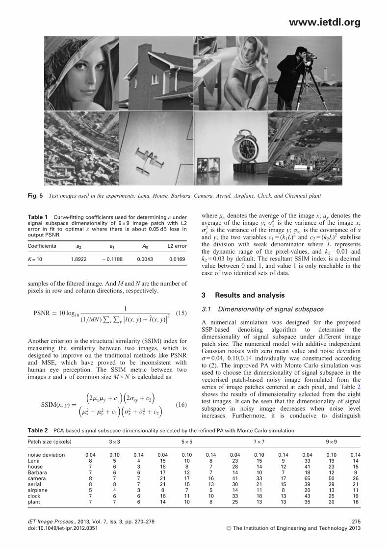
guided filter and the traditional guided filter are shownas a function of noise deviation σ and 5 × 5 imageneighbourhoods, respectively. The proposed PCA guidedfilter finds the guide image in the following way: itreconstructs the guide image from noisy image byprojecting onto the corresponding eigenvectors of the 10largest singular values. In our experiments, the eight testimages selected from the USC-SIPI Image database [36] areshown in Fig. 5. Five of them, that is, ‘Lena’, ‘house’,‘Barbara’, ‘camera’ and ‘aerial’, were corrupted with variantnoise deviation σ = 0.04, 0.07, 0.10, 0.12, 0.14 were used to

Fig. 3 Comparison of PSNR (dB) as a function of the parameter εfor improved PCA guided filter and the traditional guided filterindividually applied on the normalised noisy lena image


verify the relationship between optimal parameter ε andnoise deviation σ. The optimal value of ε behaves in a verypredictable way with the use of noise deviation σ. As canbe seen, for a fixed window size, for example, 5 × 5 pixels,the relationship between optimal ɛ and σ is approximatelyquadratic relation for both the proposed PCA guided filterand the traditional guided filter using variant test images,but the coefficients of quadratic functions are different.Therefore, under the given r × r image neighbourhoods andthe dimensionality K of factors for noisy images, we utilisethe quadratic fit to estimate the parameter ɛ as a function ofnoise deviation σ.

1 = a2s2 + a1s+ a0 (14)

Muresan and Parks [34] employed the smallest singular valueof sample image neighbourhoods to estimate noise deviationwith quite small bias error, that is, s = lP/255. Thereforethis noise estimate technique can be used together with (14)to automatically select a suboptimal parameter ε valueunder the given image neighbourhood size r × r anddimensionality of factors K for a single noisy image.Through five training images, Table 1 illustrates thequadratic fit parameters of the proposed PCA guided filterfor the chosen dimensionality K = 10 of factors in thepatch-based noisy images with block size 9 × 9 pixels, andalso shows the quadratic fitting error and resulting loss ofPSNR in the denoised image. It can be seen that the PSNRloss resulting from using the automatic parameter εselection in substitution for the optimal ε is negligiblebecause of the smooth broad maximum PSNR outputcurves shown in Fig. 3. Therefore, the robust estimation ofthe parameter ɛ is to take much larger set of training imagesto select it by these quadratic fits. The same analysisapproach can be applied to other patch size and denoisingalgorithms. As we know, the suboptimal parameter ε alsodepends on the neighbourhood size. However, thisautomatic selection problem of the optimal neighbourhoodwindow ωk with the size r × r is difficult to solve, which isour future work to be done.

2.6 Image quality metrics

To perform a quantitative comparison between theperformances of the different denoising algorithms, wecomputed some well-known noise-reduction full referencequality metrics [37–39]. The first measure criterion is thePSNR, defined by (15), where I(x, y) denotes the samplesof the normalised original image, I(x, y) denotes the

Fig. 4 Suboptimal parameterε value as a functionof noise deviationσ


www.ietdl.org

Fig. 5 Test images used in the experiments: Lena, House, Barbara, Camera, Aerial, Airplane, Clock, and Chemical plant

samples of the filtered image. AndM and N are the number ofpixels in row and column directions, respectively.

PSNR = 10 log101

(1/MN )∑

x

∑y I (x, y)− I(x, y)∣∣ ∣∣2 (15)

Another criterion is the structural similarity (SSIM) index formeasuring the similarity between two images, which isdesigned to improve on the traditional methods like PSNRand MSE, which have proved to be inconsistent withhuman eye perception. The SSIM metric between twoimages x and y of common size M ×N is calculated as

SSIM(x, y) =2mxmy + c1

( )2sxy + c2

( )

m2x + m2

y + c1

( )s2x + s2

y + c2

( ) (16)

Table 1 Curve-fitting coefficients used for determining ε undersignal subspace dimensionality of 9 × 9 image patch with L2error in fit to optimal ε where there is about 0.05 dB loss inoutput PSNR

Coefficients a2 a1 A0 L2 error

K = 10 1.8922 − 0.1188 0.0043 0.0169


where μx denotes the average of the image x; μy denotes theaverage of the image y; s2

x is the variance of the image x;s2y is the variance of the image y; σxy is the covariance of x

and y; the two variables c1 = (k1L)2 and c2 = (k2L)

2 stabilisethe division with weak denominator where L representsthe dynamic range of the pixel-values, and k1 = 0.01 andk2 = 0.03 by default. The resultant SSIM index is a decimalvalue between 0 and 1, and value 1 is only reachable in thecase of two identical sets of data.

3 Results and analysis

3.1 Dimensionality of signal subspace

A numerical simulation was designed for the proposedSSP-based denoising algorithm to determine thedimensionality of signal subspace under different imagepatch size. The numerical model with additive independentGaussian noises with zero mean value and noise deviationσ = 0.04, 0.10,0.14 individually was constructed accordingto (2). The improved PA with Monte Carlo simulation wasused to choose the dimensionality of signal subspace in thevectorised patch-based noisy image formulated from theseries of image patches centered at each pixel, and Table 2shows the results of dimensionality selected from the eighttest images. It can be seen that the dimensionality of signalsubspace in noisy image decreases when noise levelincreases. Furthermore, it is conducive to distinguish

Table 2 PCA-based signal subspace dimensionality selected by the refined PA with Monte Carlo simulation

Patch size (pixels) 3 × 3 5 × 5 7 × 7 9 × 9

noise deviation 0.04 0.10 0.14 0.04 0.10 0.14 0.04 0.10 0.14 0.04 0.10 0.14Lena 8 5 4 15 10 8 23 15 9 33 19 14house 7 6 3 18 8 7 28 14 12 41 23 15Barbara 7 6 6 17 12 7 14 10 7 18 12 9camera 8 7 7 21 17 16 41 33 17 65 50 26aerial 8 8 7 21 15 13 30 21 15 39 29 21airplane 5 4 3 8 7 5 14 11 8 20 13 11clock 7 6 6 16 11 10 33 18 13 43 25 19plant 7 7 6 14 10 8 25 13 13 35 20 16


www.ietdl.org
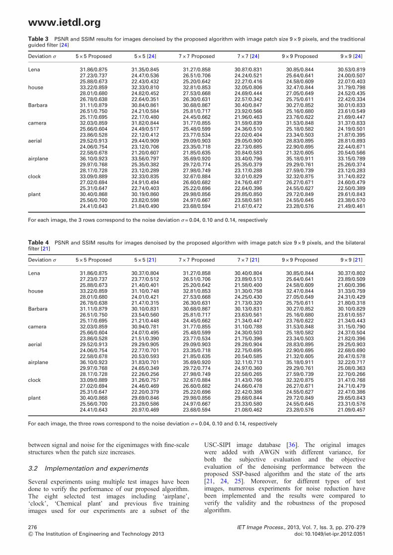
Table 3 PSNR and SSIM results for images denoised by the proposed algorithm with image patch size 9 × 9 pixels, and the traditionalguided filter [24]
Deviation σ 5 × 5 Proposed 5 × 5 [24] 7 × 7 Proposed 7 × 7 [24] 9 × 9 Proposed 9 × 9 [24]

Lena 31.86/0.875 31.35/0.845 31.27/0.858 30.87/0.831 30.85/0.844 30.53/0.81927.23/0.737 24.47/0.536 26.51/0.706 24.24/0.521 25.64/0.641 24.00/0.50725.88/0.673 22.43/0.432 25.20/0.642 22.27/0.416 24.58/0.609 22.07/0.403

house 33.22/0.859 32.33/0.810 32.81/0.853 32.05/0.806 32.47/0.844 31.79/0.79828.01/0.680 24.82/0.452 27.53/0.668 24.69/0.444 27.05/0.649 24.52/0.43526.78/0.638 22.64/0.351 26.30/0.631 22.57/0.342 25.75/0.611 22.42/0.334

Barbara 31.11/0.879 30.84/0.861 30.68/0.867 30.40/0.847 30.27/0.852 30.01/0.83326.51/0.750 24.21/0.584 25.81/0.717 23.92/0.566 25.16/0.680 23.61/0.54925.17/0.695 22.17/0.480 24.45/0.662 21.96/0.463 23.76/0.622 21.69/0.447

camera 32.03/0.859 31.82/0.844 31.77/0.855 31.59/0.839 31.53/0.848 31.37/0.83325.66/0.604 24.49/0.517 25.48/0.599 24.36/0.510 25.18/0.582 24.19/0.50123.86/0.528 22.12/0.412 23.77/0.534 22.02/0.404 23.34/0.503 21.87/0.395

aerial 29.52/0.913 29.44/0.909 29.09/0.903 29.05/0.900 28.83/0.895 28.81/0.89324.06/0.754 23.12/0.706 23.35/0.718 22.73/0.685 22.90/0.695 22.44/0.67122.58/0.678 21.20/0.607 21.85/0.635 20.84/0.583 21.32/0.605 20.54/0.566

airplane 36.10/0.923 33.56/0.797 35.69/0.920 33.40/0.796 35.18/0.911 33.15/0.78929.97/0.768 25.35/0.382 29.72/0.774 25.35/0.379 29.29/0.761 25.26/0.37428.17/0.728 23.12/0.289 27.98/0.749 23.17/0.288 27.59/0.739 23.12/0.283

clock 33.09/0.889 32.33/0.835 32.67/0.884 32.01/0.829 32.32/0.875 31.74/0.82227.02/0.694 24.91/0.494 26.60/0.682 24.76/0.487 26.27/0.671 24.60/0.47925.31/0.647 22.74/0.403 25.22/0.696 22.64/0.396 24.55/0.627 22.50/0.389

plant 30.40/0.868 30.19/0.860 29.98/0.856 29.85/0.850 29.72/0.849 29.61/0.84325.56/0.700 23.82/0.598 24.97/0.667 23.58/0.581 24.55/0.645 23.38/0.57024.41/0.643 21.84/0.490 23.68/0.594 21.67/0.472 23.28/0.576 21.49/0.461

For each image, the 3 rows correspond to the noise deviation σ = 0.04, 0.10 and 0.14, respectively

Table 4 PSNR and SSIM results for images denoised by the proposed algorithm with image patch size 9 × 9 pixels, and the bilateralfilter [21]

Deviation σ 5 × 5 Proposed 5 × 5 [21] 7 × 7 Proposed 7 × 7 [21] 9 × 9 Proposed 9 × 9 [21]

Lena 31.86/0.875 30.37/0.804 31.27/0.858 30.40/0.804 30.85/0.844 30.37/0.80227.23/0.737 23.77/0.512 26.51/0.706 23.89/0.513 25.64/0.641 23.89/0.50925.88/0.673 21.40/0.401 25.20/0.642 21.58/0.400 24.58/0.609 21.60/0.396

house 33.22/0.859 31.10/0.748 32.81/0.853 31.30/0.758 32.47/0.844 31.33/0.75928.01/0.680 24.01/0.421 27.53/0.668 24.25/0.430 27.05/0.649 24.31/0.42926.78/0.638 21.47/0.315 26.30/0.631 21.73/0.320 25.75/0.611 21.80/0.318

Barbara 31.11/0.879 30.10/0.831 30.68/0.867 30.13/0.831 30.27/0.852 30.10/0.82926.51/0.750 23.54/0.560 25.81/0.717 23.63/0.561 25.16/0.680 23.61/0.55725.17/0.695 21.21/0.448 24.45/0.662 21.34/0.447 23.76/0.622 21.34/0.443

camera 32.03/0.859 30.94/0.781 31.77/0.855 31.10/0.788 31.53/0.848 31.15/0.79025.66/0.604 24.07/0.495 25.48/0.599 24.30/0.503 25.18/0.582 24.37/0.50423.86/0.528 21.51/0.390 23.77/0.534 21.75/0.396 23.34/0.503 21.82/0.396

aerial 29.52/0.913 29.29/0.905 29.09/0.903 29.28/0.904 28.83/0.895 29.25/0.90324.06/0.754 22.77/0.701 23.35/0.718 22.75/0.695 22.90/0.695 22.68/0.69022.58/0.678 20.53/0.593 21.85/0.635 20.54/0.585 21.32/0.605 20.47/0.578

airplane 36.10/0.923 31.83/0.701 35.69/0.920 32.11/0.713 35.18/0.911 32.22/0.71729.97/0.768 24.65/0.349 29.72/0.774 24.97/0.360 29.29/0.761 25.08/0.36328.17/0.728 22.26/0.256 27.98/0.749 22.58/0.265 27.59/0.739 22.70/0.266

clock 33.09/0.889 31.26/0.757 32.67/0.884 31.43/0.766 32.32/0.875 31.47/0.76827.02/0.694 24.46/0.469 26.60/0.682 24.66/0.478 26.27/0.671 24.71/0.47925.31/0.647 22.20/0.379 25.22/0.696 22.42/0.386 24.55/0.627 22.47/0.386

plant 30.40/0.868 29.69/0.846 29.98/0.856 29.68/0.844 29.72/0.849 29.65/0.84325.56/0.700 23.28/0.586 24.97/0.667 23.33/0.580 24.55/0.645 23.31/0.57624.41/0.643 20.97/0.469 23.68/0.594 21.08/0.462 23.28/0.576 21.09/0.457

For each image, the three rows correspond to the noise deviation σ = 0.04, 0.10 and 0.14, respectively

between signal and noise for the eigenimages with fine-scalestructures when the patch size increases.

3.2 Implementation and experiments

Several experiments using multiple test images have beendone to verify the performance of our proposed algorithm.The eight selected test images including ‘airplane’,‘clock’, ‘Chemical plant’ and previous five trainingimages used for our experiments are a subset of the


USC-SIPI image database [36]. The original imageswere added with AWGN with different variance, forboth the subjective evaluation and the objectiveevaluation of the denoising performance between theproposed SSP-based algorithm and the state of the arts[21, 24, 25]. Moreover, for different types of testimages, numerous experiments for noise reduction havebeen implemented and the results were compared toverify the validity and the robustness of the proposedalgorithm.


www.ietdl.org

Experiments are performed on well-known 8-bit grey-scaletest images. We compared our work based on PSNR andSSIM, which is a method for measuring the similaritybetween two images (the original and the processed images)reportedly assessing image qualities more reliably thanPSNR [39]. In this experiment, the test images weredegraded by additive Gaussian noise with zero means anddifferent deviations σ = 0.04, 0.10 and 0.14, respectively.The performances of our developing algorithm were

Table 5 Comparison for the computation time between theproposed algorithm and the denoising methods in [21, 24],respectively

Methods [24] [21] Proposed

time, s 0.25 1.52 1.63


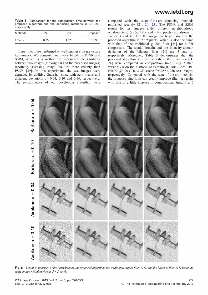
compared with the state-of-the-art denoising methodspublished recently [21, 24, 25]. The PSNR and SSIMresults for test images under different neighbourhoodwindows (e.g. 5 × 5, 7 × 7 and 9 × 9 pixels) are shown inTables 3 and 4. Here the image patch size used in theproposed algorithm is 9 × 9 pixels, which is also the samewith that of the traditional guided filter [24] for a faircomparison. The spatial-domain and the intensity-domaindeviation of the bilateral filter [21] are 3 and σ,respectively. Moreover, Table 5 demonstrates that theproposed algorithm and the methods in the literatures [21,24] were compared in computation time using Matlabversion 7.8 on the platform of Pentium(R) Dual-Core CPUE5800 @3.20 GHz 2 GB cache for 256 × 256 test images,respectively. Compared with the state-of-the-art methods,the proposed algorithm can greatly improve filtering resultswith loss of a little increase in computational time. Fig. 6

Fig. 6 Visual comparison of the noisy images, the proposed algorithm, the traditional guided filter [24], and the bilateral filter [21] using thesame image neighbourhoods 5 × 5 pixels


www.ietdl.org
shows the detailed results of noise removal for the proposedmethod, the traditional guided filter [24], and the bilateralfilter [21] for the fragments of the normalised ‘Barbara’ and‘Airplane’ images. As seen from the experimental results,the proposed algorithm, which can reach better results thanthe state-of-the-art methods on noise removal, works wellfor a wide variety of noisy images, and can remove morenoise, restore clearer images, preserve more details andsharper edges.
4 Conclusion and future work

In this paper, we presented a novel denoising algorithm whichis based on the guided filter. The reference image of theproposed algorithm is reconstructed from the noisy imageprojected onto the lower-dimensional signal subspace basedon global PCA determined by refined parallel analysiswith Monte Carlo simulation for the high-dimensionalpatch-based noisy image matrix. We have addressed theproblem of determining the dimensionality of the signalsubspace in the noisy image under certain image patch sizeand the automatic selection of the optimal parameters of theguided image filter. The smallest singular value of thepatch-based image matrix by SVD is used to estimateimage noise deviation, which is adopted to automaticallychoose the optimal parameter value of the improved guidedfilter algorithm. The relationship between noise deviationand the optimal parameter value can be established byfitting polynomial model through pre-computing the outputmaximum PSNR of test image corrupted with differentnoise level. Although the proposed algorithm isgeneralisation of the guided image filter with small loss ofcomputational efficiency, it was observed that our SSP-based denoising algorithm performs much better than thetraditional guided image filter and other state-of-the-artsmethods both visually and quantitatively. Moreover, thereconstructed image from the lower-dimensional projectionsusing the improved PA approach with Monte Carlosimulations can also be easily applied on other denoisingand filtering algorithms for weight function calculation.Finally, the automatic selection of the optimal imageneighbourhood size of the denoising algorithm and thefurther reduction of computation time are left for our futureresearch.

5 Acknowledgments

This work was supported by National Basic ResearchProgram (973 Program) of China under ContractNo. 2009CB320907, National Natural Science Foundationof China under contract No. 61101078, and Doctoral Fundof Ministry of Education of China under contractNo. 20110001120117. The authors would like to thank theeditors and reviewers gratefully for their efforts, comments,and recommendations, which have led to a substantialimprovement of the technical content and the presentationquality of this manuscript.

6 References

1 Nahi, N.E.: ‘Role of recursive estimation in statistical imageenhancement’, Proc. IEEE, 1972, 60, (7), pp. 872–877

2 Lev, A., Zucker, S.W., Rosenfeld, A.: ‘Iterative enhancement of noisyimages’, IEEE Trans. Syst., Man Cybern., 1977, 7, (6), pp. 435–442

3 Lee, J.S.: ‘Digital image enhancement and noise filtering by use of localstatistics’, IEEE Trans. Pattern Anal. Mach. Intell., 1980, 2, (2),pp. 165–168


4 Donoho, D.L.: ‘De-noising by soft-thresholding’, IEEE Trans. Inf.Theory, 1995, 41, (3), pp. 613–627

5 Simoncelli, E.P., Adelson, E.H.: ‘Noise removal via Bayesian waveletcoring’. Proc. of Third IEEE Int. Conf. on Image Processing,September 1996, pp. 379–382

6 Mihcak, M.K., Kozintsev, I., Ramchandran, K., Moulin, P.: ‘Lowcomplexity image denoising based on statistical modeling ofwavelet coefficients’, IEEE Signal Process. Lett., 1999, 6, (12), pp.300–303

7 Li, X., Orchard, M.: ‘Spatially adaptive image denoising underovercomplete expansion’, Int. Conf. on Image Processing(ICIP), 2000,3, pp. 300–303

8 Chang, S.G., Yu, B., Vetterli, M.: ‘Adaptive wavelet thresholding forimage denoising and compression’, IEEE Trans. Image Process.,2000, 9, (9), pp. 1532–1546

9 Starck, J.L., Cands, E.J., Donoho, D.L.: ‘The curvelet transform forimage denoising’, IEEE Trans. Image Process., 2002, 11, (6),pp. 670–684

10 Portilla, J., Strela, V., Wainwright, M.J., Simoncelli, E.P.: ‘Imagedenoising using scale mixtures of gaussians in the wavelet domain’,IEEE Trans. Image Process., 2003, 12, (11), pp. 1338–1351

11 Bhutada, G.G., Anand, R.S., Saxena, S.C.: ‘Image enhancement bywavelet-based thresholding neural network with adaptive learningrate’, IET Image Process., 2011, 5, (7), pp. 573–582

12 Buades, A., Coll, B., Morel, J.M.: ‘A review of image denoisingalgorithms, with a new one’, Multiscale Model. Simul., 2005, 4, (2),pp. 490–530

13 Tasdizen, T.: ‘Principal neighborhood dictionaries for non-local meansimage denoising’, IEEE Trans. Image Process., 2009, 18, (12),pp. 2649–2260

14 Weissman, T., Ordentlich, E., Seroussi, G., Verd, S., Weinberger, M.:‘Universal discrete denoising: Known channel’, IEEE Trans. Inf.Theory, 2005, 51, (1), pp. 5–28

15 Awate, S.P., Whitaker, R.T.: ‘Unsupervised, information-theoretic,adaptive image filtering for image restoration’, IEEE Trans. PatternAnal. Mach. Intell., 2006, 28, (3), pp. 364–376

16 Aharon, M., Elad, M., Bruckstein, A.M.: ‘K-SVD: An algorithm fordesigning of overcomplete dictionaries for sparse representation’,IEEE Trans. Signal Process., 2006, 54, (11), pp. 4311–4322

17 Elad, M., Aharon, M.: ‘Image denoising via sparse and redundantrepresentations over learned dictionaries’, IEEE Trans. ImageProcess., 2006, 15, (12), pp. 3736–3745

18 Hirakawa, K., Parks, T.W.: ‘Image denoising using total least squares’,IEEE Trans. Image Process., 2006, 15, (9), pp. 2730–2742

19 Foi, A., Katkovnik, V., Egiazarian, K.: ‘Pointwise shape-adaptive DCTfor high-quality denoising and deblocking of grayscale andcolor images’, IEEE Trans. Image Process., 2007, 16, (5), pp.1395–1411

20 Dabov, K., Foi, A., Katkovnik, V., Egiazarian, K.: ‘Image denoising bysparse 3D transform-domain collaborative filtering’, IEEE Trans. ImageProcess., 2007, 16, (8), pp. 2080–2095

21 Tomasi, C., Manduchi, R.: ‘Bilateral filtering for gray and colorimages’. Proc. of the Sixth Int. Conf. on Computer Vision, 1998, pp.839–846

22 Takeda, H., Farsiu, S., Milanfar, P.: ‘Kernel regression for imageprocessing and reconstruction’, IEEE Trans. Image Process., 2007,16, (2), pp. 349–366

23 Zhang, Y., Ai, Y., Dai, K., Zhang, G.: ‘Grey model via polynomial forimage denoising’, J. Grey Syst., 2010, 22, (2), pp. 117–128

24 He, K., Sun, J., Tang, X.: ‘Guided image filtering’, Comput. Vis. –ECCV 2010, Lect. Notes Comput. Sci., 2010, 6311, pp. 1–14

25 Rydell, J., Knutsson, H., Borga, M.: ‘Bilateral filtering of fMRI data’,IEEE J. Sel. Top. Signal Process., 2008, 2, (6), pp. 891–896

26 Ding, Y., Chung, Y.C., Simonetti, O.P.: ‘A method to assess spatiallyvariant noise in dynamic MR image series’, Magn. Reson. Med.,2010, 63, (3), pp. 782–789

27 Park, S.W., Kang, M.G.: ‘Image denoising filter based onpatch-based difference refinement’, Opt. Eng., 2012, 51, (6), pp.067007:1–13

28 Chul, L., Chulwoo, L., Chang-Su, K.: ‘An MMSE approach to nonlocalimage denoising: Theory and practical implementation’, J. Vis.Commun. Image Represent., 2012, 23, (3), pp. 476–490

29 Zhang, L., Li, X., Zhang, D.: ‘Image denoising and zooming under thelinear minimum mean square-error estimation framework’, IET ImageProcess., 2012, 6, (3), pp. 273–283

30 Pablo, B., Martin, E., Marcus, M.: ‘Guided image filtering for interactivehigh-quality global illumination’, Comput. Graph. Forum, 2011, 30, (4),pp. 1361–1368

31 Xiao, C., Gan, J.: ‘Fast image Dehazing using guided joint bilateralfilter’, Vis. Comput., 2012, 28, (6–8), pp. 713–721


www.ietdl.org
32 Horn, J.L.: ‘A rationale and test for the number of factors in factor
analysis’, Psychomerica, 1965, 30, (2), pp. 179–18533 Jorgensen, K.W., Hansen, L.K.: ‘Model selection for Gaussian kernel

PCA denoising’, IEEE Trans. Neural Netw. Learn. Syst., 2012, 23,(1), pp. 163–168

34 Muresan, D.D., Parks, T.W.: ‘Adaptive principal components and imagedenoising’, IEEE Int. Conf. Image Process. (ICIP), 2003, 1,pp. 101–104

35 Azzabou, N., Paragios, N., Guichard, F.: ‘Image denoising based onadapted dictionary computation’, IEEE Int. Conf. Image Process.(ICIP), 2007, 3, pp. III-109–III-112


36 Weber, A.: ‘The USC-SIPI image database’, June 1, 2012, available athttp://www.sipi.usc.edu/database/

37 Chikkerur, S., Sundaram, V., Reisslein, M., Karam, L.J.: ‘Objectivevideo quality assessment methods: a classification, review, andperformance comparison’, IEEE Trans. Broadcast., 2011, 57, (2),pp. 165–182

38 Huynh-Thu, Q., Ghanbari, M.: ‘Scope of validity of PSNR in image/video quality assessment’, Electron. Lett., 2008, 44, (13), pp. 800–801

39 Wang, Z., Bovik, A.C., Sheikh, H.R., et al.: ‘Image quality assessment:from error visibility to structural similarity’, IEEE Trans. ImageProcess., 2004, 13, (4), pp. 600–612


Guided image filtering using signal subspace projection

Documents

Transcript of Guided image filtering using signal subspace projection