
An analysis of convergence for a learning version of the subspace method
Upload
khangminh22Category
view
3download
0
1
Discriminative Linear and
Multilinear Subspace Methods
Dacheng TAO
A Thesis Submitted in Partial Fulfilment of the Requirements
for the Degree of Doctor of Philosophy
October 2006
School of Computer Science and Information Systems

2
This thesis is submitted to the School of Computer Science and Information
Systems, Birkbeck College, University of London in partial fulfilment of the
requirements for the degree of Doctor of Philosophy. I hereby declare that this
thesis is my own work and except where otherwise stated. This submission has
not been submitted for a degree to any other university or institution.
Dacheng TAO
School of Computer Science and Information Systems
Birkbeck College
University of London

3
To my family.
1
Table of Contents
Table of Contents .................................................................................................... 1
List of Figures ......................................................................................................... 1
List of Tables........................................................................................................... 7
Abstract ................................................................................................................... 9
Acknowledgement................................................................................................. 10
1. Introduction ..................................................................................................... 1
1.1 Thesis Organization............................................................................. 6
1.2 Publications ....................................................................................... 10
2. Discriminative Linear Subspace Methods..................................................... 11
2.1 Principal Component Analysis.......................................................... 14
2.2 Linear Discriminant Analysis............................................................ 17
2.3 General Averaged Divergences Analysis.......................................... 32
2.4 Geometric Mean for Subspace Selection .......................................... 38
2.5 Kullback–Leibler Divergence based Subspace Selection ................. 41
2.6 Comparison using Synthetic Data ..................................................... 50
2.7 Statistical Experiments ...................................................................... 56
2.8 Real–World Experiments .................................................................. 63
2.9 Summary ........................................................................................... 65
3. Discriminative Multilinear Subspace Method............................................... 66
3.1 Tensor Algebra .................................................................................. 70
3.2 The Relationship between LSM and MLSM .................................... 77
3.3 Tensor Rank One Analysis................................................................ 79
3.4 General Tensor Analysis ................................................................... 83
3.5 Two Dimensional Linear Discriminant Analysis.............................. 87
3.6 General Tensor Discriminant Analysis ............................................. 90
3.7 Manifold Learning using Tensor Representations ............................ 96
3.8 GTDA for Human Gait Recognition ................................................. 99
3.9 Summary ......................................................................................... 120
4. Supervised Tensor Learning........................................................................ 121
4.1 Convex Optimization based Learning............................................. 124
4.2 Supervised Tensor Learning: A Framework ................................... 129
2
4.3 Supervised Tensor Learning: Examples.......................................... 136
4.4 Iterative Feature Extraction Model based on Supervised Tensor
Learning....................................................................................................... 152
4.5 Experiments..................................................................................... 156
4.6 Summary ......................................................................................... 188
5. Thesis Conclusion ....................................................................................... 189
6. Appendices .................................................................................................. 194
6.1 Appendix for Chapter 2................................................................... 194
6.2 Appendix for Chapter 3................................................................... 205
References ........................................................................................................... 211
1
List of Figures
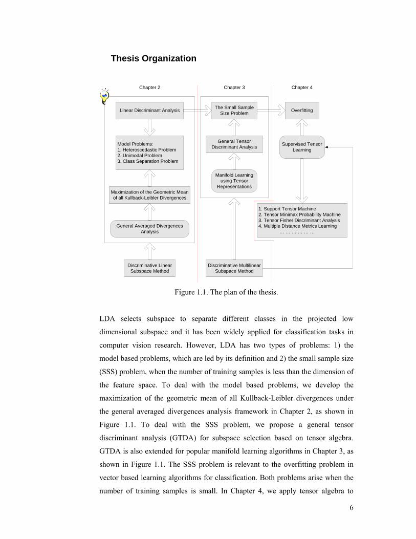
Figure 1.1. The plan of the thesis. ........................................................................... 6
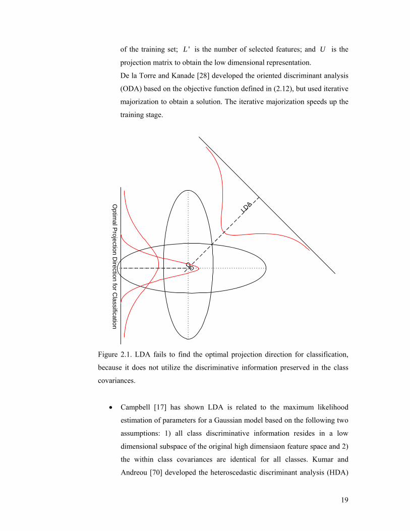
Figure 2.1. LDA fails to find the optimal projection direction for classification,
because it does not utilize the discriminative information preserved in the class
covariances. ........................................................................................................... 19
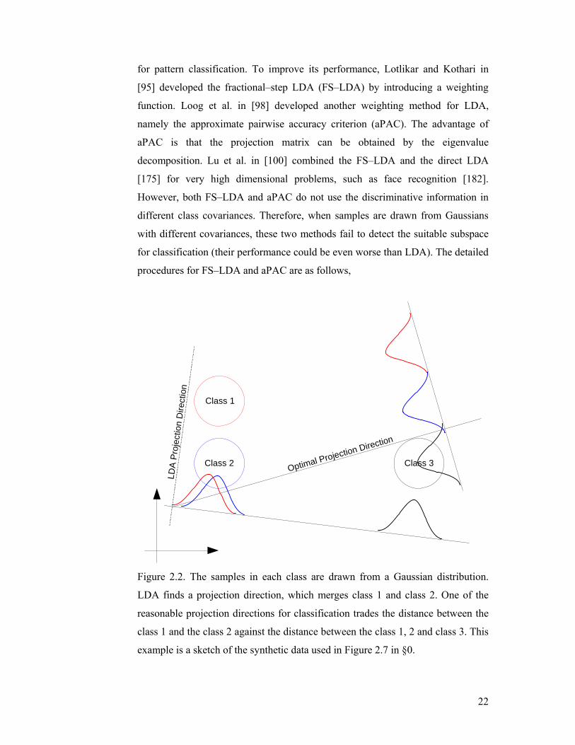
Figure 2.2. The samples in each class are drawn from a Gaussian distribution.
LDA finds a projection direction, which merges class 1 and class 2. One of the
reasonable projection directions for classification trades the distance between the
class 1 and the class 2 against the distance between the class 1, 2 and class 3. This
example is a sketch of the synthetic data used in Figure 2.7 in §2.6.3. ................ 22
Figure 2.3. The geometric setting for Bregman divergence.................................. 33
Figure 2.4. Heteroscedastic example: in this figure, from left to right, from top to
bottom, there are nine subfigures showing the projection directions (indicated by
lines in each subfigure) obtained using LDA, HDA, aPAC, WLDA, FS–LDA,
HLDA, ODA, MGMKLD(0), and MGMKLD(1). In this experiment, the linear
classifier ( ) ( )1ˆ ˆˆ ˆ lnTi i i ix m x m−− Σ − + Σ is applied as the classification method
after a subspace selection procedure, where ˆ im and ˆiΣ are the estimated ith
class mean and covariance matrix in the lower dimensional space, respectively.
The training classification errors of these methods are 0.3410, 0.2790, 0.3410,
0.3410, 0.3430, 0.2880, 0.2390, 0.2390, and 0.2390, respectively....................... 51
Figure 2.5. The maximization of the geometric mean of the normalized
divergences is not sufficient for subspace selection.............................................. 52
Figure 2.6. Multimodal problem: in this figure, from left to right, from top to
bottom, there are nine subfigures, which show the projection directions (indicated
by lines in each subfigure) by using LDA, HDA, aPAC, FS–LDA(3), FS–LDA(8),
HLDA, MODA, M–MGMKLD(0), and M–MGMKLD(1). In this experiment, the
linear classifier ( ) ( )1ˆ ˆˆ ˆ lnTi i i ix m x m−− Σ − + Σ is applied as the classification
method after a subspace selection procedure, where ˆ im and ˆiΣ are the
estimated ith class mean and covariance matrix in the lower dimensional space,
respectively. The training classification errors of these methods are 0.0917,
2
0.0167, 0.0917, 0.0917, 0.0917, 0.0167, 0.0083, 0.0083, and 0.0083, respectively.
............................................................................................................................... 53
Figure 2.7. Class separation problem: in this figure, from left to right, from top to
bottom, there are nine subfigures to describe the projection directions (indicated
by lines in each subfigure) by using LDA, HDA, aPAC, WLDA, FS–LDA,
HLDA, ODA, MGMKLD(0), and MGMKLD(5). In this experiment, the linear
classifier ( ) ( )1ˆ ˆˆ ˆ lnTi i i ix m x m−− Σ − + Σ is applied as the classification method
after a subspace selection procedure, where ˆ im and ˆiΣ are the estimated ith
class mean and covariance matrix in the lower dimensional space, respectively.
The training classification errors of these methods are 0.3100, 0.3033, 0.2900,
0.3033, 0.0567, 0.3100, 0.3100, 0.1167, and 0.0200, respectively. MGMKLD(5)
finds the best projection direction for classification. ............................................ 55
Figure 2.8. Class separation problem: in this figure, from left to right, there are
three subfigures to describe the projection directions (indicated by lines in each
subfigure) by using aPAC, FS–LDA, and MGMKLD(5). In this experiment, the
linear classifier ( ) ( )1ˆ ˆˆ ˆ lnTi i i ix m x m−− Σ − + Σ is applied as the classification
method after a subspace selection procedure, where ˆ im and ˆiΣ are the
estimated ith class mean and covariance matrix in the lower dimensional space,
respectively. The training classification errors of these methods are 0.1200,
0.1733, and 0.0267, respectively. MGMKLD(5) finds the best projection direction
for classification. ................................................................................................... 55
Figure 2.9. Data Generation Model. In this model, 1 4w = , 2 0w = , 3 4w = − ,
4 4w = , 5 4w = , 2k = , ( )1 1 201Tm km w= +r r , 2 200Tm =
r , ( )[ ]3 3 10 100 ,1 Tm km w= +r r ,
( )[ ]4 4 10 101 ,0 Tm km w= +r r , and ( )[ ]5 5 5 5 5 51 ,0 ,1 ,0 Tm km w= +
r r . .............................. 56
Figure 2.10. Initial values: From left to right, from top to bottom, the subfigures
show the mean value and the corresponding standard deviation of the KL
divergence between the class i and the class j of these 50 different initial values in
the 10th (50th, 100th, and 1000th) training iterations. Because there are 5 classes in
the training set, there are 20 KL divergences to examine. The circles in each
subfigure show the mean values of the KL divergences for 50 different initial
values. The error bars show the corresponding standard deviations. For better
visualization, the scale for showing the standard deviations is 10 times larger than
3
the vertical scale in each subfigure. The standard deviations of these 20 KL
divergences approach 0 as the number of training iterations increases. ............... 60
Figure 2.11. MGMKLD(2c) has no nest structure property.................................. 62
Figure 2.12. Samples in the USPS database [53]. ................................................. 63
Figure 3.1. A gray level face image is a second order tensor, i.e., a matrix. Two
indices are required for pixel locations. The face image comes from
http://www.merl.com/projects/images/face–rec.gif. ............................................. 66
Figure 3.2. A color image is a third order tensor, which is also a data cuboid,
because three indices are required to locate elements. Two indices are used for
pixel locations and one index is used to local the color information (e.g., R, G, and
B). .......................................................................................................................... 66
Figure 3.3. A color video shot is a fourth order tensor. Four indices are used to
locate elements. Two indices are used for pixel locations; one index is used to
locate the color information; and the other index is used for time. The video shot
comes from http://www–nlpir.nist.gov/projects/trecvid/. ..................................... 67
Figure 3.4. A third order tensor 1 2 3L L LR × ×∈X . ...................................................... 70
Figure 3.5. The mode–1, mode–2, and mode–3 matricizing of a third order tensor 3 2 2R × ×∈X . ............................................................................................................. 71
Figure 3.6. The mode–2 product of a third order tensor 1 2 3L L LR × ×∈X and a matrix 2 2L LU R ′ ×∈ results in a new tensor 1 2 3L L LR ′× ×∈Y . ................................................. 73
Figure 3.7. The HOSVD of a third order tensor 1 2 3L L LR × ×∈X .............................. 74
Figure 3.8. The best rank one approximation to a third order tensor 1 2 3L L LR × ×∈X .
............................................................................................................................... 79
Figure 3.9. The best ( )1 2 3rank , ,R R R− approximation of a third order tensor
1 2 3L L LR × ×∈X . .......................................................................................................... 83
Figure 3.10. The columns show the averaged gait images of nine different people
in the Gallery of the USF database described in §3.8.2.1. The four rows in the
figure from top to bottom are based on images taken from the Gallery, ProbeB,
ProbeH, and ProbeK, respectively. The averaged gait images in a single column
come from the same person................................................................................. 100
Figure 3.11. The real part of Gabor functions with five different scales and eight
different directions. ............................................................................................. 101

4
Figure 3.12. Gabor gait: the rows show different scales and the columns show
different directions for an averaged gait image................................................... 102
Figure 3.13. Three new methods for averaged gait image representation using
Gabor functions: GaborS, GaborD, and GaborSD. ............................................. 103
Figure 3.14. The thirteen columns are Gallery gait, ProbeA gait, ProbeB gait,
ProbeC gait, ProbeD gait, ProbeE gait, ProbeF gait, ProbeG gait, ProbeH gait,
ProbeI gait, ProbeJ gait, ProbeK gait, and ProbeL gait, respectively. From the first
row to the last row are the original gait, GaborD (from 0 to 4), GaborS (from 0 to
7), and GaborSD, respectively. The Gallery gait and ProbeA – ProbeI gaits are
described in Section 3.8.2.1................................................................................. 105
Figure 3.15. The averaged gait extraction and the dissimilarity measure. .......... 108
Figure 3.16. Recognition performance comparison for rank one evaluation. From
top–left to bottom, in each of the thirteen subfigures (Probes A, B, C, D, E, F, G,
H, I, J, K, L, and the average performance), there are eleven bars, which
correspond to the performance of HMM, IMED+LDA, LDA, LDA+Fusion,
2DLDA+LDA, GTDA+LDA(H), GTDA+LDA, Gabor+GTDA+LDA(H),
GaborD+GTDA+LDA(H), GaborS+GTDA+LDA(H), and GaborSD+GTDA+
LDA(H), respectively.......................................................................................... 116
Figure 3.17. Recognition performance comparison for rank five evaluation. From
top–left to bottom, in each of the thirteen subfigures (Probes A, B, C, D, E, F, G,
H, I, J, K, L, and the average performance), there are ten bars, which correspond
to the performance of IMED+LDA, LDA, LDA+Fusion, 2DLDA+LDA, GTDA
+LDA(H), GTDA+LDA, Gabor+GTDA+LDA(H), GaborD+GTDA+LDA(H),
GaborS+GTDA+LDA(H), and GaborSD+GTDA+LDA(H), respectively......... 118
Figure 3.18. Experimental based convergence justification for the alternating
projection method for GTDA. The x–coordinate is the number of training
iterations and the y–coordinate is the error value Err, as defined in Step 6 in Table
3.6. From left to right, these four sub–figures show how Err changes with the
increasing number of training iterations with different threshold values (88%,
90% 92% and 94%) defined in (3.37). ................................................................ 119
Figure 4.1. Tensor based learning machine vs. vector based learning machine. 122
Figure 4.2. The geometric interpretation of the optimal solution *wr in D for a
convex optimization problem defined in (4.3). ................................................... 125
5
Figure 4.3. The geometric interpretation of the optimal solution *wr in D for
LP defined in (4.5)............................................................................................... 126
Figure 4.4. The geometric interpretation of the optimal solution *wr in D for
QP defined in (4.6). ............................................................................................. 127
Figure 4.5. The third order tensor example for the alternating projection in STL.
............................................................................................................................. 133
Figure 4.6. SVM maximizes the margin between positive and negative training
samples. ............................................................................................................... 136
Figure 4.7. MPM separates positive samples from negative samples by
maximizing the probability of the correct classification for future samples. The
intersection point minimizes the maximum of the Mahalanobis distances between
positive and negative samples, i.e., it has the same Mahalanobis distances to the
mean of the positive samples and the mean of the negative samples.................. 142
Figure 4.8. FDA separates positive samples from negative samples by maximizing
the symmetric Kullback–Leibler divergence between two classes under the
assumption that the two classes share the same covariance matrix. ................... 146
Figure 4.9. DML obtains a metric, such that “k–nearest neighbors always belong
to the same class while examples from different classes are separated by a large
margin”................................................................................................................ 149
Figure 4.10. Iterative feature extraction model for third order tensors. .............. 152
Figure 4.11. Attention model for image representation. ..................................... 156
Figure 4.12. Example images from the tiger category. ....................................... 157
Figure 4.13. Example images from the leopard category.................................... 158
Figure 4.14. One hundred ROIs in the tiger category. ........................................ 159
Figure 4.15. One hundred ROIs in the leopard category..................................... 160
Figure 4.16. TMPM converges effectively. ........................................................ 162
Figure 4.17. TMPM is stable with different initial values. ................................. 163
Figure 4.18. First 10 EigenGaits (the first column), first 10 FisherGaits (the
second column), first 10 TR1AGaits (the third column), and first 10 TR1DAGaits
(the fourth column). From the figure, we can see that EigenGaits and FisherGaits
are dense, while TR1AGaits and TR1DAGaits are sparse, because they take the
structure information into account to reduce the number of unknown parameters
in discriminant learning....................................................................................... 166
6
Figure 4.19. GBL task: TR1DA performances, convergence, and parameters
(feature dimension and ς ) analysis. Detailed explanation is in §4.5.2.............. 171
Figure 4.20. GAL task: TR1DA performances, convergence, and parameters
(feature dimension and ς ) analysis. Detailed explanation is in §4.5.2.............. 173
Figure 4.21. CBL task: TR1DA performances, convergence, and parameters
(feature dimension and ς ) analysis. Detailed explanation is in §4.5.2.............. 175
Figure 4.22. CAL task: TR1DA performances, convergence, and parameters
(feature dimension and ς ) analysis. Detailed explanation is in §4.5.2.............. 177
Figure 4.23. GBBL task: TR1DA performances, convergence, and parameters
(feature dimension and ς ) analysis. Detailed explanation is in §4.5.2.............. 179
Figure 4.24. GBAL task: TR1DA performances, convergence, and parameters
(feature dimension and ς ) analysis. Detailed explanation is in §4.5.2.............. 181
Figure 4.25. CBBL task: TR1DA performances, convergence, and parameters
(feature dimension and ς ) analysis. Detailed explanation is in §4.5.2.............. 183
Figure 4.26. CBAL task: TR1DA performances, convergence, and parameters
(feature dimension and ς ) analysis. Detailed explanation is in §4.5.2.............. 185
7
List of Tables
Table 2.1. Fractional–Step Linear Discriminant Analysis .................................... 23
Table 2.2. Linear Discriminant Analysis via Generalized Singular Value
Decomposition....................................................................................................... 26
Table 2.3. Linear Discriminant Analysis via QR Decomposition......................... 28
Table 2.4. General Averaged Divergences Analysis for Subspace Selection ....... 35
Table 2.5. Optimization procedure for MGMKLD............................................... 42
Table 2.6. Optimization procedure for M–MGMKLD. ........................................ 44
Table 2.7: Averaged classification errors (the mean for 800 experiments) of LDA,
HDA, aPAC, WLDA, FS–LDA, HLDA, ODA, MGMKLD(0), and
MGMKLD(2c). (The nearest neighbour rule)....................................................... 58
Table 2.8: Standard deviations of classification errors for 800 experiments of
LDA, HDA, aPAC, WLDA, FS–LDA, HLDA, ODA, MGMKLD(0), and
MGMKLD(2c). (The nearest neighbour rule)....................................................... 58
Table 2.9: Averaged classification errors (the mean for 800 experiments) of LDA,
HDA, aPAC, WLDA, FS–LDA, HLDA, ODA, MGMKLD(0), and
MGMKLD(2c). (The linear classifier ( ) ( )1ˆ ˆˆ ˆlnT
i i i ix m x m−− Σ − + Σr r r r ) ................. 59
Table 2.10: Standard deviations of classification errors for 800 experiments of
LDA, HDA, aPAC, WLDA, FS–LDA, HLDA, ODA, MGMKLD(0), and
MGMKLD(2c). (The linear classifier ( ) ( )1ˆ ˆˆ ˆlnT
i i i ix m x m−− Σ − + Σr r r r ) ................. 59
Table 2.11. Performances (classification errors) of linear methods on the USPS
database. (The nearest neighbour rule).................................................................. 64
Table 2.12. Performances (error rates) of kernel methods on the USPS database. A
nine dimensional feature space is selected for each algorithm. (The nearest
neighbour rule) ...................................................................................................... 64
Table 3.1. Alternating Projection for the Higher–Order Singular Value
Decomposition....................................................................................................... 75
Table 3.2. Alternating Projection for the Best Rank One Approximation ............ 80
Table 3.3. Alternating Projection for the Tensor Rank One Analysis .................. 81
Table 3.4. Alternating Projection for the Best Rank– ( )1 2, , MR R RL
Approximation....................................................................................................... 84
Table 3.5. Alternating Projection for General Tensor Analysis............................ 85
8
Table 3.6. Alternating Projection for General Tensor Discriminant Analysis...... 94
Table 3.7. Computational complexities of the alternating projection method based
optimization procedure of GTDA with Gabor/GaborD/GaborS/GaborSD
representations..................................................................................................... 106
Table 3.8. Twelve probe sets for challenge experiments. ................................... 107
Table 3.9. Rank one recognition rates for human gait recognition. .................... 113
Table 3.10. Rank five recognition rates for human gait recognition................... 114
Table 4.1. Alternating Projection for the Supervised Tensor Learning .............. 131
Table 4.2. Alternating Projection for the Tensor Rank One Discriminant Analysis
............................................................................................................................. 154
Table 4.3. TMPM vs. MPM ................................................................................ 161
Table 4.4. Parameters in convergence examination for eight probes.................. 169
Table 4.5. Rank One recognition precision for eight probes............................... 169
Table 4.6. Rank five recognition precision for eight probes. .............................. 169
9
Abstract
Linear discriminant analysis (LDA) sheds light on classification tasks in computer
vision. However, classification based on LDA can perform poorly in applications
because LDA has: 1) the heteroscedastic problem, 2) the multimodal problem, 3)
the class separation problem, and 4) the small sample size (SSS) problem. In this
thesis, the first three problems are called the model based problems because they
arise from the definition of LDA. The fourth problem arises when there are too
few training samples. The SSS problem is also known as the overfitting problem.
To address the model based problems, a new criterion is proposed: maximization
of the geometric mean of the Kullback–Leibler (KL) divergences and the
normalized KL divergences for subspace selection when samples are sampled
from Gaussian mixture models. The new criterion reduces all model based
problems significantly, as shown by a large number of empirical studies.
To address the SSS problem in LDA, a general tensor discriminant analysis
(GTDA) is developed. GTDA makes better use of the structure information of the
objects in vision research. GTDA is a multilinear extension of a modified LDA. It
involves the estimation of a series of projection matrices in projecting an object in
the form of a tensor from a high dimensional feature space to a low dimensional
feature space. Experiments on human gait recognition demonstrate that GTDA
combined with LDA and nearest neighbor rule outperforms competing methods.
Based on the work above, the standard convex optimization based approach to
machine learning is generalized to the supervised tensor learning (STL)
framework, in which tensors are accepted as input. The solution to STL is
obtained in practice using an alternating projection algorithm. This generalization
reduces the overfitting problem when there are only a few training samples. An
empirical study confirms that the overfitting is reduced.

10
Acknowledgement
Professor Stephen J. Maybank is an excellent advisor and friend! During the two
years for my PhD study, I owed him a lot because I have obtained everlasting
helps from him when I was confused; I have obtained inspirations from him when
I was depressed; and I have obtained rigorous comments from him when I was not
correct on mathematics. I am anxious to have his comments, because they are my
precious stairs, which shape my research from style to content. I would like to
express my deepest gratitude to Steve.
I would like to thank my second supervisor and friend Dr. Xuelong Li for his
discussions, suggestions, and encouragements. With Xuelong’s help, I can do my
research here directly and I can become familiar with London with little effort.
I appreciate my external examiner Professor Andrew Blake at Microsoft Research
Cambridge Lab and internal examiner Professor Shaogang Gong at Queen Mary
for their time reviewing this thesis, their patience for my PhD viva, their
constructive comments to refine this thesis, and their encouragements for my
work.
I would like to thank my fantastic collaborator and friend Professor Xindong Wu
(UVM) for his valuable and interesting suggestions.
I would like to thank my fantastic collaborator and friend Professor Christos
Faloutsos (CMU) and Mr. Jimeng Sun (CMU) for an interesting collaboration
work on tensor analysis for streaming data.
I would like to thank Professor Mario Figueiredo (Instituto Superior Técnico) for
his explanation on the boundary problem in the training procedure of the Gaussian
mixture model.
I need to thank the financial support from the Overseas Research Students Award
Scheme (ORSAS), the Birkbeck College, and the School of Computer Science

11
and Information Systems. Without them, I have no chance to finish my PhD in
UK.
I would also like to thank Mr. Phil Gregg, Mr. Graham Sadler, Mr. Andrew
Watkins, and Mr. Phil Docking for their help on computing resources. Without
their help, I would not have obtained my experimental results in time. I occupied
many computers simultaneously (usually more than five) in the laboratory many
times.
I would like to thank Ms. Betty Walters and Ms. Gilda Andreani for their help in
administration during my study. I thank all members in the department for their
encouragements and suggestions.
I would like to thank my good friends, Dr. Renata Camargo (Birkbeck), Mr.
Liangliang Cao (UIUC), Dr. Yuzhong Chen (Tokyo), Dr. Jun Cheng (CUHK),
Ms. Victoria Gagova (Birkbeck), Dr. Qi Li (UDEL), Dr. Zhifeng Li (CUHK), Mr.
Wei Liu (CUHK), Ms. Ju Luan (CUHK), Mr. Bo Luo (PSU), Mr. Xiaolong Ma
(SUNY-SB), Dr. Mingli Song (ZJU), Mr. Jimeng Sun (CMU), Mr. Wei Wang
(UC-Davis), Mr. Xiaogang Wang (MIT), Dr. Yonggang Wen (MIT), Dr. Hui
Xiong (Rutgers), Dr. Dong Xu (Columbia), Mr. Jin Xu (NLPR), Mr. Tianqiang
Yuan (CUHK), Dr. Dell Zhang (Birkbeck), etc. Moreover, I especially need to
thank Mr. Xiaolong Ma for his friendly support. I also need to thank Dr. Qi Li for
useful discussions.
Finally, I owe my family a lot for many things. I thank all my family members for
their extreme understanding and infinite support of my PhD study and academic
pursuits.
1
1. Introduction
Linear subspace methods [58] have been used as an important pre–processing step
in many applications of classification for dimension reduction or subspace
selection, because of the so called curse of dimensionality [7]. The aim of the
linear subspace methods is to project the original high dimensional feature space
to a low dimensional subspace. Many methods have been proposed for selecting
the low dimensional subspace, e.g., principal component analysis (PCA) [64] and
linear discriminant analysis (LDA) [103]. PCA finds a subspace, which minimizes
reconstruction error, while LDA finds a subspace, which separates different
classes in the projected low dimensional space.
In this thesis, we mainly focus on discriminative linear subspace methods,
especially on LDA, because LDA has been widely used in classification tasks in
computer vision research, such as image segmentation [97], relevance feedback in
content based image retrieval [139][152][153][154], image database indexing
[113], video shots classification [43], medical image analysis [116], object
recognition and categorization [54], natural scene classification [156], face
recognition [158][118][34][168], gait recognition [46][78][79][166][165][142],
fingerprint recognition [59], palmprint recognition [62][179], texture
classification [133], and hand writing classification [119].
The following view of LDA is taken in this thesis: when samples are drawn from
different Gaussian distributions [60] with identical covariance matrices, LDA
maximizes the arithmetic mean of the Kullback–Leibler (KL) [21] divergences
between all pairs of distributions after projection into a subspace. From this point
of view, LDA has the following problems: 1) heteroscedastic problem
[29][28][35][70][61][81][99]: LDA ignores the discriminative information, which
is present when the covariance matrices change between classes; 2) multimodal
problem [51][28]: each class is modelled by a single Gaussian distribution; and 3)
class separation problem [103][95][96][99][146]: LDA merges classes which are
close together in the original feature space. We call these three problems model
based problems, because they are part of the limitations of the definition of LDA.
Apart from the model based problems, LDA also has the small sample size (SSS)
problem [38][49][139][123][19][175][55][173][174][180], when the number of
2
training samples is less than the dimension of the feature space. In the LDA
model, two scatter matrices are calculated. These are the between class scatter
matrix [39] and the within class scatter matrix [39]. The between class scatter
matrix measures the separation between different classes. The larger the volume
(e.g., the trace value) of the matrix is, the better the different classes are separated.
The within class scatter matrix describes the scatter of samples around their
respective class centers. The smaller the volume of the matrix is, the closer the
samples are to their respective class centers. LDA finds a subspace, which
maximizes the ratio between the trace of the projected between class scatter
matrix and the trace of the projected within class scatter matrix. The solution is
given by an eigenvalue decomposition [44] of the product of the inverse of the
within class scatter matrix and the between class scatter matrix. In many real
applications, LDA cannot be applied in this straightforward way, because the rank
of the within class scatter is deficient [47], i.e., the inverse of the matrix does not
exist.
To deal with the model based problems, it is important to develop a flexible
framework. Because LDA is equal to the maximization of the arithmetic mean of
the KL divergences when samples are obtained from different Gaussian
distributions with identical covariances, we develop a general averaged
divergences analysis framework, which extends LDA in two ways: 1)
generalizing the KL divergences to the Bregman divergence [14], which is a
general distortion measure of probability distributions and 2) generalizing the
arithmetic mean to the generalized mean [48], which includes as special cases a
large number of mean functions, e.g., the arithmetic mean, the geometric mean
[20], and the harmonic mean [1][48]. Because this framework takes different
covariance matrices into account, it can make better use of the information in
heteroscedastic data. Then we combine the Gaussian Mixture Model (GMM) [30]
with the framework to reduce the multimodal problem. In applications, LDA
tends to merge classes, which are close in the original high dimensional space.
This problem is reduced with the proposed general averaged divergences analysis
framework by using geometric mean for subspace selection. Three criteria for
subspace selection are described: 1) maximization of the geometric mean of the
divergences; 2) maximization of the geometric mean of normalized divergences;
and 3) maximization of the geometric mean of all divergences (both the
3
divergences and the normalized divergences). Experiments with computer
generated data and digitized hand writing [53] show that the combination of the
geometric mean based criteria and the KL divergence significantly reduces the
heteroscedastic problem, the multimodal problem and the class separation
problem.
To deal with the SSS problem, the following two steps are conducted:
1) the LDA criterion is replaced by the difference between the trace of the
between class scatter matrix in the projected subspace and the weighted trace
of the within class scatter matrix in the projected subspace. The new criterion
is named the differential scatter discriminant criterion (DSDC) [143][149].
The relationship between LDA and DSDC is discussed in detail in Chapter 2;
2) In computer vision research, samples are often tensors, i.e.,
multidimensional arrays. For example, the averaged gait image [45][91],
which is the feature used for gait recognition, is a matrix, or a second order
tensor; a face image, is also a matrix in face recognition [182]; a color image
[54] in object recognition is a third order tensor or a three dimensional array;
and a color video shot (a color image sequence) [43] in video retrieval is a
forth order tensor or a four dimensional array. Therefore, DSDC is
reformulated through operations in multilinear algebra [115][75] or tensor
algebra [115][75]. That is we substitute the multilinear algebra operations,
e.g., the tensor product, the tensor contraction, and the mode product, for the
linear algebra operations, e.g., the matrix product, the matrix transpose, and
the trace operation. Then we can directly replace the vectors, which are used
to represent vectorized samples, with tensors, which are used to represent the
original samples.
The combination of the two steps described above is named the general tensor
discriminant analysis (GTDA) [144][147]. By this replacement, the SSS problem
can be significantly reduced, because we need not to estimate a large projection
matrix at a time. That is we estimate a series of small projection matrices
iteratively by using the alternating projection method, which obtains each small
projection matrix with all the other fixed projection matrices in an iterative way,
i.e., an alternating projection method for optimization decouples a projection
matrix from the others. In each iteration, the number of unknown parameters (the
size of a projection matrix) in GTDA is much less than that of in LDA.
4
GTDA is motivated by the successes of the tensor rank one analysis (TR1A)
[132], general tensor analysis (GTA) [75][162][171], and the two dimensional
LDA (2DLDA) [174] for face recognition. The benefits of GTDA are: 1)
reduction of the SSS problem for subsequent classification, e.g., by LDA; 2)
preservation of discriminative information in training tensors, while PCA, TR1A,
and GTA do not guarantee this; 3) provision with stable recognition rates because
the optimization algorithm of GTDA converges, while that of 2DLDA does not;
and 4) acceptance of the general tensors as input, while 2DLDA only accepts
matrices as input.
We then apply the proposed GTDA to appearance [82] based human gait
recognition [45][46][91][92]. For appearance based gait recognition, the averaged
gait images are suited for human gait recognition, because: 1) the averaged gait
images of the same person share similar visual effects under different
circumstances; and 2) the averaged gait images of different people even under the
same circumstance are very different. Motivated by the successes of Gabor
function [32][80] based image decompositions for image understanding and
object recognition, we develop three different Gabor function based image
representations [144]: 1) the sum of Gabor functions over directions based
representation (GaborD), 2) the sum of Gabor functions over scales based
representation (GaborS), and 3) the sum of Gabor functions over scales and
directions based representation (GaborSD). These representations are applied to
recognize people from their averaged gait images. A large number of experiments
were carried out to evaluate the effectiveness (recognition rate) of gait recognition
based on the following three successive steps: 1) the Gabor/GaborD/GaborS/
GaborSD image representations, 2) GTDA to extract features from the Gabor/
GaborD/GaborS/GaborSD image representations, and 3) applying LDA for
recognition. The proposed methods achieve sound performance for gait
recognition based on the USF HumanID Database [126]. Experimental
comparisons are made with nine state of the art classification methods
[46][66][126][167][173] in gait recognition.
Finally, vector based learning1 is extended to accept tensors as input. This results
in the supervised tensor learning (STL) framework [149][150], which is the
1 Vector based learning means the traditional classification technique, which accepts vectors as input. In vector based learning, a projection vector Lw R∈
r and a bias b R∈ are learnt to
5
multilinear extension of the convex optimization [11] based learning. To obtain
the solution of an STL based learning algorithm, an alternating projection method
is designed. Based on STL and its alternating projection optimization algorithm,
we illustrate some examples. That is we extend the soft margin support vector
machine (SVM) [161][15], the nu–SVM [130][128], the least squares SVM
[137][138], the minimax probability machine (MPM) [74][135], the Fisher
discriminant analysis (FDA) [37][30][69], the distance metric learning (DML)
[169] to their tensor versions, which are the soft margin support tensor machine
(STM), the nu–STM, the least squares STM, the tensor MPM (TMPM) [150], the
tensor FDA (TFDA), and the multiple distance metrices learning (MDML),
respectively. With STL, we also introduce a method for feature extraction through
an iterative way [132] and develop the tensor rank one discriminant analysis
(TR1DA) [145][143] as an example. The experiments for image classification
demonstrate TMPM reduces the overfitting problem in MPM. The experiments
for the elapsed time problem in human gait recognition show TR1DA is more
effective than PCA, LDA, and TR1A.
determine the class label of a sample Lx R∈r according to a linear decision function
( ) sign Ty x w x b⎡ ⎤= +⎣ ⎦r r r . The wr and b are obtained based on a learning model, e.g., minimax
probability machine (MPM), which is based on N training samples associated with labels { },L
i ix R y∈r , where iy is the class label, { }1, 1iy ∈ + − , and 1 i N≤ ≤ .
6
Thesis Organization
Model Problems:1. Heteroscedastic Problem2. Unimodal Problem3. Class Separation Problem
The Small Sample Size Problem Overfitting
Supervised Tensor Learning
Discriminative Linear Subspace Method
Discriminative Multilinear Subspace Method
Maximization of the Geometric Mean of all Kullback-Leibler Divergences
Linear Discriminant Analysis
General Averaged Divergences Analysis
1. Support Tensor Machine2. Tensor Minimax Probability Machine3. Tensor Fisher Discriminant Analysis4. Multiple Distance Metrics Learning … … … … … …
Chapter 2 Chapter 3 Chapter 4
General Tensor Discriminant Analysis
Manifold Learning using Tensor
Representations
Figure 1.1. The plan of the thesis.
LDA selects subspace to separate different classes in the projected low
dimensional subspace and it has been widely applied for classification tasks in
computer vision research. However, LDA has two types of problems: 1) the
model based problems, which are led by its definition and 2) the small sample size
(SSS) problem, when the number of training samples is less than the dimension of
the feature space. To deal with the model based problems, we develop the
maximization of the geometric mean of all Kullback-Leibler divergences under
the general averaged divergences analysis framework in Chapter 2, as shown in
Figure 1.1. To deal with the SSS problem, we propose a general tensor
discriminant analysis (GTDA) for subspace selection based on tensor algebra.
GTDA is also extended for popular manifold learning algorithms in Chapter 3, as
shown in Figure 1.1. The SSS problem is relevant to the overfitting problem in
vector based learning algorithms for classification. Both problems arise when the
number of training samples is small. In Chapter 4, we apply tensor algebra to
7
extend vector based learning algorithms to accept tensors as input to reduce the
overfitting problem. A number of examples are provided in this Chapter, as shown
in Figure 1.1.
In Chapter 2, we review two important linear subspace methods [58], namely
principal component analysis (PCA) [64] and linear discriminant analysis (LDA)
[103]. We then analyze the problems of LDA and review some extensions [19]
[28][29][38][49][51][55][61][70][95][96][99][103][123][139][173][174][175][18
0] of LDA to reduce these problems. We also give a new point of view [146] on
discriminative subspace selection and develop a new framework for subspace
selection, the general averaged divergences analysis [146]. This framework allows
a range of different criteria for assessing subspaces. Based on the new framework,
we investigate geometric mean [20] for discriminative subspace selection and
develop a method for the maximization of the geometric mean of all Kullback–
Leibler (KL) [21] divergences (MGMKLD) [146] by combining the maximization
of the geometric mean of all divergences and the KL divergence for subspace
selection. A large number of experiments are conducted to demonstrate the
effectiveness of the new discriminative subspace selection method compared with
LDA and its representative extensions.
In Chapter 3, we focus on multilinear subspace methods, because the objects in
computer vision research are often tensors [75]. Firstly, tensor algebra [115][75]
is briefly introduced. It is the mathematical fundamental material of this Chapter.
After that, unsupervised learning techniques, such as TR1A [132] and GTA [75]
[162][171], are reviewed. We also give a brief introduction of 2LDA [174].
Motivated by the success of 2DLDA in face recognition, we then develop GTDA,
which includes the following parts: 1) the LDA criterion is replaced by DSDC
[143][149]. The relationship between LDA and DSDC is discussed in detail; and
2) DSDC is reformulated through operations in multilinear algebra [115][75].
Based on the reformulated DSDC, vectors can be replaced with tensors, i.e.,
retaining the original format of samples; 3) an alternating projection optimization
procedure is developed to obtain the solution of GTDA; 4) provide the
mathematical proof of the convergence of the alternating projection optimization
procedure for calculating the projection matrices; and 5) the computational
complexity is analyzed. Finally, the proposed GTDA combined with LDA and the
nearest neighbour classifier is utilized for appearance based human gait
8
recognition [45][46][91][92]. Compared with previous algorithms, the newly
presented algorithms achieve better recognition rates.
In Chapter 4, a supervised tensor learning (STL) framework [149][150] is
developed based on the similar idea to reduce the SSS problem in Chapter 3. We
first introduce convex optimization [11] and convex optimization based learning.
Then we propose the STL framework associated with the alternating projection
method for optimization. Based on STL and its alternating projection optimization
algorithm, we generalize the support vector machine (SVM) [161][15][130][128]
[137][138], the minimax probability machine (MPM) [74][135], the Fisher
discriminant analysis (FDA) [37][30] [69], and the distance metric learning
(DML) [169], as the support tensor machine, the tensor minimax probability
machine, the tensor Fisher discriminant analysis, and the multiple distance metrics
learning, respectively. We also propose an iterative feature extraction method
based on STL. As an example, we develop the tensor rank one discriminant
analysis (TR1DA). Experiments are conducted based on the tensor minimax
probability machine and TR1DA.
Chapter 5 concludes.
The main contributions of the thesis are three folds:
1. Develop a discriminative subspace selection framework, i.e., general
averaged divergences analysis. Based on this framework, a special case,
i.e., maximization of the geometric mean of all Kullback–Leibler (KL)
divergences, is given to significantly reduce the class separation problem
raised by imbalanced distributions of KL divergences between different
classes. Moreover, it is also compatible with the heteroscedastic property
of data and deals with samples drawn from mixture of Gaussians naturally.
Empirical studies demonstrate that it outperforms LDA and its
representative extensions;
2. Develop the general tensor discriminant analysis (GTDA) to reduce the
small sample size (SSS) problem. Unlike all existing tensor based
discriminative subspace selection algorithms, GTDA converges in the
training stage. Moreover, a full mathematical proof is given. To our best
knowledge, this is the first work in the world to give both a converged
algorithm and a mathematical proof. Again, this proof can be also applied
to justify whether a tensor based algorithm converges or not by checking
9
the convexity of its objective function. By applying GTDA to human gait
recognition, we achieve the state-of-the-art recognition accuracy; and
3. By applying tensor algebra to vector based learning, we finally develop a
supervised tensor learning framework. The significance of the framework
is we can conveniently generalize different vector based classifiers to
tensor based classifiers to reduce the over–fitting problem. For example,
we generalize the support vector machine to the support tensor machine
and give out the error bound; we generalize the Fisher discriminant
analysis and the minimax probability machine to the tensor Fisher
discriminant analysis and the tensor minimax probability machine,
respectively, to overcome the matrix singular problem; and we generalize
distance metric learning to multiple distance metrics learning to make it
computable for appearance based recognition tasks. Finally, an iterative
feature extraction model is given based on supervised tensor learning.
Empirical studies show the power of supervised tensor learning and the
iterative feature extraction model.
10
Publications
The research of this thesis has resulted in the following research papers:
1. D. Tao, X. Li, X. Wu, and S. J. Maybank, “General Tensor Discriminant Analysis and Gabor Features for Gait Recognition,” IEEE Transactions on Pattern Analysis and Machine Intelligence (TPAMI), 2007. [Chapter 3]
2. D. Tao, X. Li, X. Wu, and S. J. Maybank, “Tensor Rank One Discriminant Analysis,” Submitted to IEEE Transactions on Pattern Analysis and Machine Intelligence (TPAMI). (Under Major Revision) [Chapter 4]
3. D. Tao, X. Li, X. Wu, and S. J. Maybank, “General Averaged Divergences Analysis,” Submitted to IEEE Transactions on Pattern Analysis and Machine Intelligence (TPAMI). (Under Major Revision) [Chapter 2]
4. D. Tao, X. Li, and S. J. Maybank, “Negative Samples Analysis in Relevance Feedback,” IEEE Transactions on Knowledge and Data Engineering (TKDE), 2007.
5. D. Tao, X. Li, W. Hu, S. J. Maybank, and X. Wu, “Supervised Tensor Learning: A Framework,” Knowledge and Information Systems (Springer), 2007. [Chapter 4]
6. D. Tao, X. Li, X. Wu, and S. J. Maybank, “Human Carrying Status in Visual Surveillance,” IEEE Int’l Conf. on Computer Vision and Pattern Recognition (CVPR), pp. 1,670–1,677, 2006. (Acceptance rate: ~20%) [Chapter 3]
7. D. Tao, X. Li, X. Wu, and S. J. Maybank, “Elapsed Time in Human Gait Recognition: A New Approach,” IEEE Int’l Conf. on Acoustics, Speech, and Signal Processing (ICASSP), vol. 2, pp. 177–180, 2006. [Chapter 4]
8. D. Tao, X. Li, W. Hu, S. J. Maybank, and X. Wu, “Supervised Tensor Learning,” IEEE Int’l Conf. on Data Mining (ICDM), pp. 450–457, 2005. (Acceptance rate: ~11%) [Chapter 4]
9. D. Tao, X. Li, W. Hu, and S. J. Maybank, “Stable Third–Order Tensor Representation for Color Image Classification,” IEEE Int’l Conf. on Web Intelligence (WI), pp. 641–644, 2005.
11
2. Discriminative Linear Subspace Methods
The linear subspace method (LSM) [2][21][50][109][107] has been developed and
demonstrated to be a powerful tool in pattern recognition and computer vision
research fields. LSM finds a matrix 'L LU R ×∈ to transform the high dimensional
sample Lx R∈r to a low dimensional sample 'Ly R∈
r , i.e., Ty U x=r r . There are
two major categories of LSM algorithms, which are focused on either feature
selection or dimension reduction, respectively. A feature selection algorithm
selects a (very small) number of most effective features from the entire feature
pool. That is the un–selected features are not utilized. In feature selection, the
linear transformation matrix U has the following properties: 1) the entries of U
are 1 or 0; 2) the inner product of any two columns of U is 0; and 3) the sum of
all entries of any column of U is 1. A dimension reduction algorithm finds
several sets of coefficients, and with each set of coefficients the original features
are weighted and summed to produce a new feature. By this means, several (less
than the number of the original features) new low dimensional samples are
“generated” to preserve as much as possible the information (e.g., reconstructive
information or discriminative information) carried by the original high
dimensional samples. In this thesis, we focus on algorithms for dimension
reduction.
From the viewpoint of modelling, LSM can be used with a large number of
models varying from reconstructive models to discriminative models. A
reconstructive LSM minimizes ( )1
Ni i Hi
L x Uy=
−∑ r r , where we have N training
samples ixr on hand; the projection matrix is U ; iyr is the low dimensional
representation of ixr ; H
⋅ is a norm; and ( )L ⋅ is a loss function [161][128].
Principal component analysis (PCA) [64] is an example of a reconstructive model.
On the other side, discriminative models, e.g., linear discriminant analysis (LDA)
[39], are utilized for classification. A discriminative LSM maximizes an objective
function to separate different classes in the projected low dimensional subspace.
Both reconstructive and discriminative models are widely used in many real–
world applications, such as biometrics [182][68], bioinformatics [31], and
multimedia information management [24][139].
12
In this Chapter, we mainly focus on the discriminative LSM, especially LDA,
because it is the most popular algorithm in dimension reduction (or subspace
selection) for classification. If samples are sampled from Gaussian distributions
with identical covariance matrices, LDA maximizes the arithmetic mean value of
the Kullback–Leibler (KL) [21] divergences between different classes. Based on
this point of view, it is not difficult to see that LDA has the following problems:
1) Heteroscedastic problem [29][28][70][61][99]: LDA models different classes
with identical covariance matrices. Therefore, it fails to take account of any
variations in the covariance matrices between different classes;
2) Multimodal problem [51][28]: In many applications, samples in each class can
not be approximated by a single Gaussian. Instead, a Gaussian mixture model
(GMM) [39][30] is required. However, LDA models each class by a single
Gaussian distribution;
3) Class separation problem [103][95][96][99][146]: In applications, distances
between different classes are different and LDA tends to merge classes which are
close together in the original feature space.
The first two problems have been well studied in the past few years and a number
of extensions of LDA have been generated to deal with them. Although some
methods [103][95][96][99] have been proposed to reduce the third problem, it is
still not well solved. In this Chapter, to further reduce the class separation
problem, we first generalize LDA to obtain a general averaged divergences
analysis, which extends LDA from two aspects: 1) the KL divergence is replaced
by the Bregman divergence [14]; and 2) the arithmetic mean is replaced by the
generalized mean function [48]. By choosing different options in 1) and 2), a
series of subspace selection algorithms are obtained, with LDA included in as a
special case.
Under the general averaged divergences analysis, we investigate the effectiveness
of geometric mean [20] based subspace selection in solving the class separation
problem. The geometric mean amplifies the effects of small divergences and at
the same time reduces the effects of large divergences. Next, the maximization of
the geometric mean of the normalized divergences is studied. This turns out not to
be suitable for subspace selection, because there exist projection matrices which
make all divergences very small and at the same time make all normalized
divergences similar in value. We therefore propose a third criterion, maximization
13
of the geometric mean of all divergences (both the divergences and the
normalized divergences) or briefly MGMD. It is a combination of the first two.
With MGMD, it is possible to develop different subspace selection methods by
choosing different divergences. In this chapter, we select the KL divergence and
assume that the samples in each class are obtained by sampling Gaussian
distributions. This results in the maximization of a function of all KL divergences
(MGMKLD). The name MGMKLD is chosen because the function is closely
related to the geometric mean of divergences. We extend MGMKLD to the case
in which the samples in each class are sampled from a Gaussian Mixture Model
[30]. This gives the multimodal extension of MGMKLD, or M–MGMKLD.
Finally, we kernelize [104][109][128][129] MGMKLD to the kernel MGMKLD
or briefly KMGMKLD. Preliminary experiments based on synthetic data and
handwriting digital data [53] show that MGMKLD achieves much better
classification rates than LDA and its several representative extensions taken from
the literature.
The Chapter is organized as follows. In §53 and §53, PCA with its kernel
extension and LDA with its representative extensions are briefly reviewed,
respectively. In §53, the general averaged divergences analysis is proposed. In
§53, the geometric mean for subspace selection is investigated. The KL
divergence based geometric mean subspace selection is developed in §53.
synthetic data based experiments, statistical experiments, and hand writing
recognition for justifying the effectiveness of linear subspace methods are given
in §53, §53, and §53, respectively. Finally, summary of this Chapter is given in
§53. Moreover, all proofs and deductions in this Chapter are given in §53.
14
Principal Component Analysis
Although PCA [64] is a reconstructive model, it has been successfully applied for
classification tasks in computer vision. It extracts the principal eigenspace
associated with a set of training samples Lix R∈r ( 1 i n≤ ≤ ). Let
( ) ( )( )11 n T
i iiS n x m x m
== − −∑ r r r r be the covariance matrix, alternatively called the
total–class scatter matrix, of all training samples ixr , where ( ) 11 n
iim n x
== ∑r r .
One solves the eigenvalue equation i iu Suλ =r r for eigenvalues 0iλ ≥ . The
projection matrix *U is spanned by the first 'L eigenvectors with the largest
eigenvalues, '1* |Li iU u∗=⎡ ⎤= ⎣ ⎦
r . If xr is a new sample, then it is projected to
( ) ( )* Ty U x m= −r r r . The vector yr is used in place of xr for representation and
classification.
PCA has the following properties. In the following description, we assume the
training samples ixr are centralized, i.e., 0m =r .
Property 2.1: PCA maximizes the variance in the projected subspace for a given
dimension 'L , i.e.,
( ) 2
1
1arg max tr arg maxn
T Ti FroU U i
U SU U xn =
= ∑ r . (2.01)
where Fro
⋅ is the Frobenius norm.
Proof: See Appendix.
Property 2.2: The principal eigenspace U in PCA diagonalizes the covariance
matrix of the training samples.
Property 2.3: PCA minimizes the reconstruction error, i.e.,
( ) 2
1
1arg max tr arg minn
T Ti i FroU U i
U SU x UU xn =
= −∑ r r . (2.02)
Proof: See Appendix.
Property 2.4: PCA decorrelates the training samples in the projected subspace.
Proof: See Appendix.
Property 2.5: PCA maximizes the mutual information between xr and yr on
Gaussian data.
Proof: See Appendix.
15
We now study the nonlinear extension of PCA, or the kernel PCA (KPCA) [129],
which takes high order stastistics of the training samples into account. Consider a
nonlinear mapping:
( ): ,L HR R x xφ φ→r ra , (2.03)
where H n= . Then, in HR , the covariance matrix is
( )( ) ( )( )1
1 n T
i ii
S x m x mnφ φ φφ φ
=
= − −∑ r r r r , (2.04)
where ( ) ( )11 n
iim n xφ φ
== ∑r r is the mean vector of all training samples in HR .
The ( ) ( )Ti ix xφ φr r is a linear operator on the range of φ in HR . Suggested by
Schölkopf et al. [128][129], the mapping is defined as ( ) ( ) ,i ix x x xφ φr r r ra . The
next step in KPCA is to find the eigenvalue decomposition on Sφ .
v S vφλ =r r . (2.05)
Because all solutions vr with 0λ ≠ are the linear combinations of ( )ixφ r ,
1 i n≤ ≤ , we have
( ) ( ), ,i ix v x S vφλ φ φ=r r r r , for all 1 i n≤ ≤ . (2.06)
Replace vr with ( )1
ni ii
xα φ=∑ r in (2.06), we have
( ) ( )
( )( ) ( )
( ) ( ) ( )
1
1
1 1
1
,
11,
1 ,
n
j i jj
n
k kn n kj i n
j kk k j
k
x x
x xn
xn
x x xn
λ α φ φ
φ φα φ
φ φ φ
=
=
= =
=
⎛ ⎞−⎜ ⎟⎝ ⎠
=⎛ ⎞
−⎜ ⎟⎝ ⎠
∑
∑∑ ∑
∑
r r
r r
r
r r r
(2.07)
for all 1 i n≤ ≤ .
In terms of the n n× kernel Gram matrix [128][129] ( ) ( ): ,ij i jK x xφ φ= =r r
( ),i jk x xr r , (2.07) is simplified as
( )( )Ti i iK K I M I M Kλ α α= − −
r r (2.08)
where iαr is a column vector and it is the eigenvectors of ( )( )TI M I M K− − ;
iλ is the eigenvalues of K ; ( ) ( ) ( ), ,i ik x z x zφ φ=r rr r is the kernel function
[128][129]; and all entries in 1 ;
n nij i j n
M m R ×
≤ ≤⎡ ⎤= ∈⎣ ⎦ are 1 n . The projection

16
matrix Λ in HR is spanned by the first ( )' 'H H H n< = iαr with the largest
eigenvalues, i.e., [ ]1i i nα
≤ ≤Λ =
r .
After obtaining the linear combination coefficients, we can project a given sample
zr to the subspace constructed by KPCA according to
( ) ( ) ( )( ) ( ) ( )1 2, , , , , , ,
T T T
Tn
X z X z
k x z k x z k x zφ φφ φΛ = Λ
= Λ ⎡ ⎤⎣ ⎦
r r
r r rr r rL
(2.09)
where ( ) 1[ ]i i nX xφ φ ≤ ≤=r .
17
Linear Discriminant Analysis
LDA [103] finds in the feature space a low dimensional subspace where the
different classes of samples remain well separated after projection to this
subspace. The subspace is spanned by a set of vectors, which are denoted as
[ ]1 ', , LU u u=r rK . It is assumed that a training set of samples is available. The
training set is divided into c classes. The ith class contains in samples
;i jxr (1 ij n≤ ≤ ), and has a mean value ( ) ;11 in
i i i jjm n x
== ∑r r . The between class
scatter matrix bS and the within class scatter matrix wS are defined by
( )( )
( )( )1
; ;1 1
1
1 i
cT
b i i ii
nc T
w i j i i j ii j
S n m m m mn
S x m x mn
=
= =
⎧ = − −⎪⎪⎨⎪ = − −⎪⎩
∑
∑∑
r r r r
r r r r (2.10)
where c is the number of classes; 1
cii
n n=
= ∑ is the size of the training set; and
( ) ;1 11 ic n
i ji jm n x
= == ∑ ∑r r is the mean vector of all training samples. Meanwhile,
( ) ( )( ); ;1 11 i Tc n
t i j i ji jS n x m x m
= == − −∑ ∑ r r r r
b wS S= + is the covariance matrix of all
samples.
The projection matrix *U of LDA is chosen to maximize the ratio between bS
and wS in the projected subspace, i.e.,
( ) ( )( )1* arg max tr T T
w bU
U U S U U S U−
= . (2.11)
The projection matrix *U is computed from the eigenvectors of 1w bS S− , under
the assumption that wS is invertible. If c equals to 2, LDA reduces to the Fisher
discriminant analysis [37]; otherwise LDA is known as the Rao discriminant
analysis [122]. Because ( )rank 1bS c≤ − , we have ' 1L c≤ − , i.e., the maximum
dimension of the projected subspace for LDA is ( )min 1, 1c L− − .
If separate classes are sampled from Gaussian distributions, all with identical
covariance matrices, then LDA maximizes the mean value of the KL divergences
between different classes. This result will be proved in §122.
LDA encounters the following problems, which are:
18
1) Heteroscedastic problem [29][28][70][61][99]: LDA discards the
discriminative information preserved in covariance matrices of different classes;
2) Multimodal problem [51][28]: LDA models each class by a single Gaussian
distribution, so it cannot find a suitable projection for classification when samples
are sampled from complex distributions, e.g., GMM;
3) Class separation problem [103][95][96][99][146]: LDA tends to merge classes
which are close together in the original feature space.
Furthermore, when the size of the training set is smaller than the dimension of the
feature space, LDA has the small sample size (SSS) problem [19][30][38][39]
[49][55][123][139][173][174][175][180].
In the following, we review some representative solutions for these problems.
Furthermore, we mention some alternatives of LDA [39], namely the
nonparametric discriminant analysis [39][40], and the kernel extension of LDA
[104][109] [128][129].
Heteroscedastic Problem
LDA does not fully utilize the discriminative information contained in the
covariances of different classes. As a result, it cannot find a suitable projection
direction when different classes share the same mean, as shown in Figure 2.1.
In the past decades, a large number of extensions based on LDA were developed
to reduce this problem. For example,
• Decell and Mayekar [29] proposed a method to obtain a subspace to
maximize the average interclass divergence, which measures the
separations between the classes. This criterion takes into account the
discriminative information preserved in the covariances of different
classes. The projection matrix *U is calculated by maximizing,
( ) (
( )( ) ) ) ( )
1
1 1;tr
1 ',
c cT T
D i ji j j i
T
j i j i
J U S U U S
m m m m U c c L
−
= = ≠
⎡ ⎛= ⎢ ⎜
⎢ ⎝⎣⎤+ − − − −⎥⎦
∑ ∑r r r r
(2.12)
where iS is the ith class covariance matrix (1 i c≤ ≤ ); imr is the mean
vector of the samples in the ith class (1 i c≤ ≤ ); c is the number of classes
19
of the training set; 'L is the number of selected features; and U is the
projection matrix to obtain the low dimensional representation.
De la Torre and Kanade [28] developed the oriented discriminant analysis
(ODA) based on the objective function defined in (2.12), but used iterative
majorization to obtain a solution. The iterative majorization speeds up the
training stage.
Optim
al Projection D
irection for Classification
LDA
Figure 2.1. LDA fails to find the optimal projection direction for classification,
because it does not utilize the discriminative information preserved in the class
covariances.
• Campbell [17] has shown LDA is related to the maximum likelihood
estimation of parameters for a Gaussian model based on the following two
assumptions: 1) all class discriminative information resides in a low
dimensional subspace of the original high dimensiaon feature space and 2)
the within class covariances are identical for all classes. Kumar and
Andreou [70] developed the heteroscedastic discriminant analysis (HDA)
20
by dropping the identical class covariances assumption. The projection
matrix *U is calculated by maximizing,
' ' ' '1
log log 2 logc
T TK L L L L i L i L
iJ n U SU n U S U n U− −
=
= + −∑ , (2.13)
where [ ]' 'L L LU U U −= is the full transformation matrix; 'LU is the
transformation submatrix to select the discriminative subspace;
( )det⋅ ⋅ ; iS is the ith class covariance matrix (1 i c≤ ≤ ); S is the
covariance matrix of all training samples; c is the number of classes of
the training set; and 'L is the number of selected features. Furthermore,
the projection matrix *U is obtained by maximizing KJ through the
gradient steepest ascent algorithm.
• Jelinek [61] proposed a different way to deal with the heteroscedastic
problem in subspace selection by the gradient steepest ascent method to
find the projection matrix *U by maximizing,
1
log logc
T TJ b i i
i
J n U S U n U S U=
= −∑ , (2.14)
where ( )det⋅ ⋅ ; iS is the covariance matrix of the ith class; bS is the
between class scatter matrix defined in (2.10); in is the number of
samples in the ith class (1 i c≤ ≤ ); c is the number of classes of the
training set; and U is the projection matrix to obtain the low dimensional
representation.
• Loog and Duin [99] introduced the Chernoff criterion to heteroscedasticize
LDA, i.e., the heteroscedastic extension of LDA (HLDA). The projection
matrix *U in HLDA is obtained by maximizing,
( ) ( )( )(( ) ( )(
( ) ( )))
1 1 21 1 2 1 2 1 2 1 2
1 1
1 21 2 1 2 1 2 1 2 1 2
1 2 1 2 1 2 1 2 1 2
1 log
log log ,
c c T
L i j w w w ij w w i j i ji j i
w w ij w w ij wi j
i w i w j w j w w
J q q S S S S S S m m m m
S S S S S S S
S S S S S S S
π π
π π
− −− − −
= = +
−− − −
− −
= × × − −
× +
− −
∑ ∑ r r r r
(2.15)
where 1
ci i kk
q n n=
= ∑ is the prior probability of the ith class; iS is the
covariance matrix of the ith class; ( )i i i jq q qπ = + ; ( )j j i jq q qπ = + ;
ij i i j jS S Sπ π= + ; wS is the within class scatter matrix defined in (2.10);
21
in is the number of samples in the ith class (1 i c≤ ≤ ); and c is the
number of classes of the training set.
The projection matrix *U of HLDA is constructed by the eigenvectors of
the LJ corresponding to the largest eigenvalues.
Multimodal problem
The direct way to deal with the multimodal problem is to model each class by a
GMM [39][30]. Two representative works are as following,
• Hastie and Tibshirani [51] combined GMM with LDA based on the fact
that LDA is equivalent to maximum likelihood classification when each
class is modelled by a single Gaussian distribution. The extension directly
replaces the original single Gaussian in each class by a Gaussian mixture
model in Campbell’s result [17], as shown in (2.13).
• De la Torre and Kanade [28] generalized ODA defined in (2.12) for the
multimodal case as the multimodal ODA (MODA) by combining it with
GMM learnt by the normalized cut [131][177]. Each class is modelled by
a GMM. The aim of MODA is to find a projection matrix *U to
maximize
( )( )( )( )
1
;
1 1 1 1 ; ; ; ; ;
trji
T Tccc c i k
MODA Ti j k l i k j l i k j l j lj i
U S U UJ
m m m m S U
−
= = = =≠
⎛ ⎞⎜ ⎟= ⎜ ⎟× − − +⎜ ⎟⎝ ⎠
∑∑∑∑ r r r r , (2.16)
where ic is the number of subclusters of the ith class; ;i kS is the
covariance matrix of the kth subcluster of the ith class; ;i kmr is the mean
vector of the kth subcluster of the ith class; c is the number of classes of
the training set; and U is the projection matrix to obtain the low
dimensional representation.
Class separation problem
One of the most severe problems in LDA is the class separation problem, i.e.,
LDA merges classes which are close together in the original feature space. As
pointed out by McLachlan in [103], Lotlikar and Kothari in [95], Loog et al. in
[98], and Lu et al. in [100], this merging of classes significantly reduces the
recognition rate. The example in Figure 2.2 shows that LDA is not always optimal
22
for pattern classification. To improve its performance, Lotlikar and Kothari in
[95] developed the fractional–step LDA (FS–LDA) by introducing a weighting
function. Loog et al. in [98] developed another weighting method for LDA,
namely the approximate pairwise accuracy criterion (aPAC). The advantage of
aPAC is that the projection matrix can be obtained by the eigenvalue
decomposition. Lu et al. in [100] combined the FS–LDA and the direct LDA
[175] for very high dimensional problems, such as face recognition [182].
However, both FS–LDA and aPAC do not use the discriminative information in
different class covariances. Therefore, when samples are drawn from Gaussians
with different covariances, these two methods fail to detect the suitable subspace
for classification (their performance could be even worse than LDA). The detailed
procedures for FS–LDA and aPAC are as follows,
LDA
Proj
ectio
n D
irect
ion
Class 1
Class 2 Class 3Optimal Projection Direction
Figure 2.2. The samples in each class are drawn from a Gaussian distribution.
LDA finds a projection direction, which merges class 1 and class 2. One of the
reasonable projection directions for classification trades the distance between the
class 1 and the class 2 against the distance between the class 1, 2 and class 3. This
example is a sketch of the synthetic data used in Figure 2.7 in §0.
23
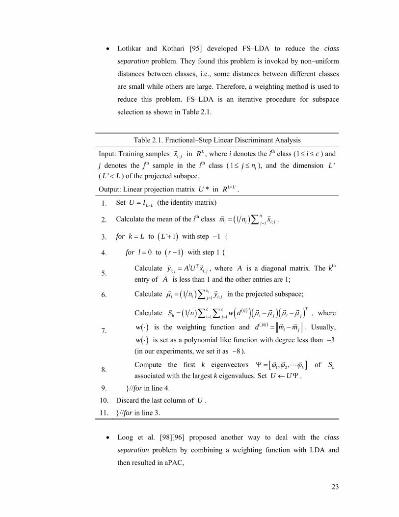
• Lotlikar and Kothari [95] developed FS–LDA to reduce the class
separation problem. They found this problem is invoked by non–uniform
distances between classes, i.e., some distances between different classes
are small while others are large. Therefore, a weighting method is used to
reduce this problem. FS–LDA is an iterative procedure for subspace
selection as shown in Table 2.1.
Table 2.1. Fractional–Step Linear Discriminant Analysis
Input: Training samples ;i jxr in LR , where i denotes the ith class (1 i c≤ ≤ ) and j denotes the jth sample in the ith class ( 1 ij n≤ ≤ ), and the dimension 'L ( 'L L< ) of the projected subapce.
Output: Linear projection matrix *U in 'L LR × .
1. Set L LU I ×= (the identity matrix)
2. Calculate the mean of the ith class ( ) ;11 in
i i i jjm n x
== ∑r r .
3. for k L= to ( )' 1L + with step 1− {
4. for 0l = to ( )1r − with step 1 {
5. Calculate ; ;
l Ti j i jy A U x=r r , where A is a diagonal matrix. The kth
entry of A is less than 1 and the other entries are 1;
6. Calculate ( ) ;11 in
i i i jjn yμ
== ∑r r in the projected subspace;
7.
Calculate ( ) ( )( )( )( )1 11
Tc c ijb i j i ji j
S n w d μ μ μ μ= =
= − −∑ ∑ r r r r , where
( )w ⋅ is the weighting function and ( )piji jd m m= −r r . Usually,
( )w ⋅ is set as a polynomial like function with degree less than 3− (in our experiments, we set it as 8− ).
8. Compute the first k eigenvectors [ ]1 2, , kϕ ϕ ϕΨ =
r r rL of bS
associated with the largest k eigenvalues. Set U U← Ψ .
9. }//for in line 4.
10. Discard the last column of U .
11. }//for in line 3.
• Loog et al. [98][96] proposed another way to deal with the class
separation problem by combining a weighting function with LDA and
then resulted in aPAC,
24
( ) ( )( )1 2 1 2
1 1
c c T
aPAC i j ij w i j i j wi j
J q q d S m m m m Sω − −
= =
= − −∑∑ r r r r , (2.17)
where ( ) ( )1T
ij i j w i jd m m S m m−= − −r r r r ;
1
ci i kk
q n n=
= ∑ is the prior
probability of the ith class; wS is the within class scatter matrix defined in
(2.10); imr is the mean vector of samples in the ith class; in is the
number of samples in the ith class (1 i c≤ ≤ ); c is the number of classes
of the training set; ( ) ( ) ( )21 2 erf 2 2x x xω = is the weighting function.
The projection matrix is 1 2* wU S −= Φ , where Φ is the matrix of leading
eigenvectors of aPACJ with the largest eigenvalues.
This combination aPACJ approximates the mean classification accuracy
(one minus Bayes error). The benefit of this method is the projection
matrix can be obtained by the eigenvalue decomposition.
The weighting function based methods are not effective for the class separation
problem, because it is not clear how to select an optimal weighting function.
Although Loog et al. [98][96] considered the Bayesian error in aPAC, it fails to
deal with the heteroscedastic problem. Even for the homoscedastic case, aPAC is
also not optimal, because it only approximats to the Bayesian error. The synthetic
data based test, shown in Figure 2.7 and Figure 2.8, demonstrates that FS–LDA
and aPAC do not often find the optimal projection direction for classification.
Small Sample Size Problem
In many practical applications, especially in biometric research, discriminant
models encounter the SSS problem [38][49][139][123][19][175][55][173][174]
[180], because the number of training samples is less than the dimension of the
feature space. To deal with this problem, a number of algorithms were proposed.
For example,
• Friedman [38] proposed the regularized discriminant analysis (RDA),
which is a classification tool to smooth out the effects of ill– or poorly–
conditioned covariance estimates due to the lack of training samples. RDA
is a combination of ridge–shrinkage [20], LDA, and quadratic discriminant
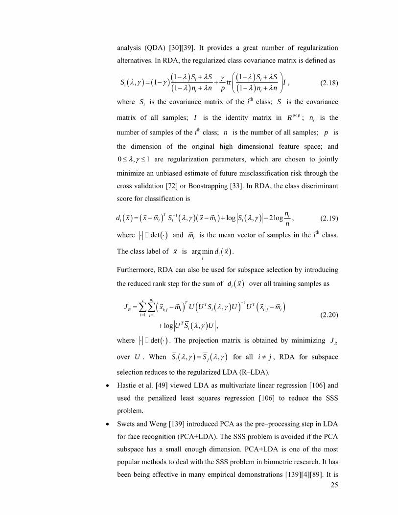
25
analysis (QDA) [30][39]. It provides a great number of regularization
alternatives. In RDA, the regularized class covariance matrix is defined as
( ) ( ) ( )( )
( )( )
1 1, 1 tr
1 1i i
ii i
S S S SS I
n n p n nλ λ λ λγλ γ γλ λ λ λ
⎛ ⎞− + − += − + ⎜ ⎟⎜ ⎟− + − +⎝ ⎠
, (2.18)
where iS is the covariance matrix of the ith class; S is the covariance
matrix of all samples; I is the identity matrix in p pR × ; in is the
number of samples of the ith class; n is the number of all samples; p is
the dimension of the original high dimensional feature space; and
0 , 1λ γ≤ ≤ are regularization parameters, which are chosen to jointly
minimize an unbiased estimate of future misclassification risk through the
cross validation [72] or Boostrapping [33]. In RDA, the class discriminant
score for classification is
( ) ( ) ( )( ) ( )1 , log , 2 logT ii i i i i
nd x x m S x m Sn
λ γ λ γ−= − − + −r r r r r , (2.19)
where ( )det⋅ ⋅ and imr is the mean vector of samples in the ith class.
The class label of xr is ( )arg min ii
d xr .
Furthermore, RDA can also be used for subspace selection by introducing
the reduced rank step for the sum of ( )id xr over all training samples as
( ) ( )( ) ( )
( )
1
; ;1 1
,
log , ,
inc T T TR i j i i i j i
i j
Ti
J x m U U S U U x m
U S U
λ γ
λ γ
−
= =
= − −
+
∑∑ r r r r
(2.20)
where ( )det⋅ ⋅ . The projection matrix is obtained by minimizing RJ
over U . When ( ) ( ), ,i jS Sλ γ λ γ= for all i j≠ , RDA for subspace
selection reduces to the regularized LDA (R–LDA).
• Hastie et al. [49] viewed LDA as multivariate linear regression [106] and
used the penalized least squares regression [106] to reduce the SSS
problem.
• Swets and Weng [139] introduced PCA as the pre–processing step in LDA
for face recognition (PCA+LDA). The SSS problem is avoided if the PCA
subspace has a small enough dimension. PCA+LDA is one of the most
popular methods to deal with the SSS problem in biometric research. It has
been being effective in many empirical demonstrations [139][4][89]. It is

26
also easy to be implemented as there are only two main steps: 1) conduct
PCA on training samples and 2) conduct LDA on the PCA pre–processed
data. PCA+LDA achieves top level performance in many applications,
such as face recognition [4][88][89], gait recognition [45][46][92], and
image retrieval [139]. The drawbacks [19][175] of this method are that the
classification performance is sensitive to the number of features selected
by PCA and PCA discards some discriminative information.
• Raudys and Duin [123] applied the pseudo–inverse [44] to the covariance
matrix in LDA as P–LDA and this utilization can reduce the SSS problem
in LDA. The projection matrix is obtained by maximizing
( ) ( )( )tr T TP w bJ U S U U S U
+= , (2.21)
where A+ means the pseudo–inversion of A , as defined in [44].
• Chen et al. [19] claimed that the most discriminative dimensions are
preserved in the null space V (the complement of the range space, i.e.,
0wS V = ) of the within class scatter matrix wS when the dimension of the
feature space is much higher than the number of training samples. First,
they project all training samples to the null space of wS . Second, PCA is
utilized on the projected samples to select the projection direction for
classification. To reduce the time complexity of this method, Cevikalp et
al. [18] developed the discriminative common vectors scheme.
• Yu and Yang [175] claimed that the null space V (or the complement of
the range space, i.e., 0bS V = ) of the between class scatter matrix bS
contains little discriminative information. Therefore, they first remove the
null space of bS and then select the projection matrix to minimize the
within class scatter matrix wS .
• Howland and Park [55] introduced the generalized singular value
decomposition (GSVD) [44] to reduce the SSS problem in LDA. The
detailed procedure is listed in Table 2.2.
Table 2.2. Linear Discriminant Analysis via Generalized Singular Value Decomposition
Input: Training samples ;i jxr in LR , where i denotes the ith class (1 i c≤ ≤ ) and
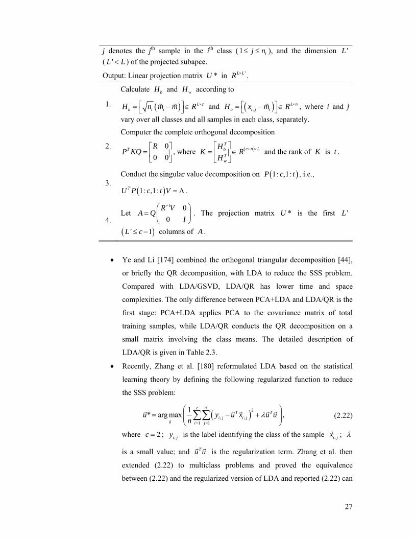
27
j denotes the jth sample in the ith class ( 1 ij n≤ ≤ ), and the dimension 'L ( 'L L< ) of the projected subapce.
Output: Linear projection matrix *U in 'L LR × .
1.
Calculate bH and wH according to
( ) L cb i iH n m m R ×⎡ ⎤= − ∈⎣ ⎦
r r and ( );L n
b i j iH x m R ×⎡ ⎤= − ∈⎣ ⎦r , where i and j
vary over all classes and all samples in each class, separately.
2.
Computer the complete orthogonal decomposition
00 0
T RP KQ
⎡ ⎤= ⎢ ⎥⎣ ⎦
, where ( )T
c n LbTw
HK R
H+ ×⎡ ⎤
= ∈⎢ ⎥⎣ ⎦
and the rank of K is t .
3. Conduct the singular value decomposition on ( )1: ,1:P c t , i.e.,
( )1: ,1:TU P c t V = Λ .
4. Let
1 00
R VA Q
I
−⎛ ⎞= ⎜ ⎟
⎝ ⎠. The projection matrix *U is the first 'L
( )' 1L c≤ − columns of A .
• Ye and Li [174] combined the orthogonal triangular decomposition [44],
or briefly the QR decomposition, with LDA to reduce the SSS problem.
Compared with LDA/GSVD, LDA/QR has lower time and space
complexities. The only difference between PCA+LDA and LDA/QR is the
first stage: PCA+LDA applies PCA to the covariance matrix of total
training samples, while LDA/QR conducts the QR decomposition on a
small matrix involving the class means. The detailed description of
LDA/QR is given in Table 2.3.
• Recently, Zhang et al. [180] reformulated LDA based on the statistical
learning theory by defining the following regularized function to reduce
the SSS problem:
( )2
; ;1 1
1* arg maxinc
T Ti j i j
u i ju y u x u u
nλ
= =
⎛ ⎞= − +⎜ ⎟
⎝ ⎠∑∑r
r r r r r , (2.22)
where 2c = ; ;i jy is the label identifying the class of the sample ;i jxr ; λ
is a small value; and Tu ur r is the regularization term. Zhang et al. then
extended (2.22) to multiclass problems and proved the equivalence
between (2.22) and the regularized version of LDA and reported (2.22) can
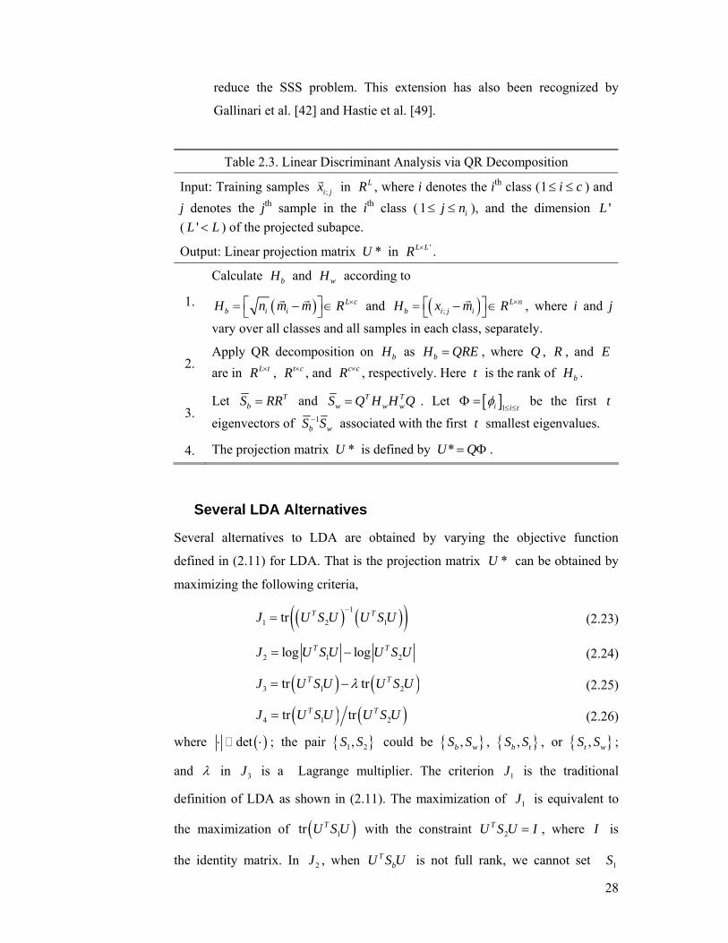
28
reduce the SSS problem. This extension has also been recognized by
Gallinari et al. [42] and Hastie et al. [49].
Table 2.3. Linear Discriminant Analysis via QR Decomposition
Input: Training samples ;i jxr in LR , where i denotes the ith class (1 i c≤ ≤ ) and j denotes the jth sample in the ith class ( 1 ij n≤ ≤ ), and the dimension 'L ( 'L L< ) of the projected subapce.
Output: Linear projection matrix *U in 'L LR × .
1.
Calculate bH and wH according to
( ) L cb i iH n m m R ×⎡ ⎤= − ∈⎣ ⎦
r r and ( );L n
b i j iH x m R ×⎡ ⎤= − ∈⎣ ⎦r , where i and j
vary over all classes and all samples in each class, separately.
2. Apply QR decomposition on bH as bH QRE= , where Q , R , and E are in L tR × , t cR × , and c cR × , respectively. Here t is the rank of bH .
3. Let T
bS RR= and T Tw w wS Q H H Q= . Let [ ]1i i t
φ≤ ≤
Φ = be the first t
eigenvectors of 1b wS S− associated with the first t smallest eigenvalues.
4. The projection matrix *U is defined by *U Q= Φ .
Several LDA Alternatives
Several alternatives to LDA are obtained by varying the objective function
defined in (2.11) for LDA. That is the projection matrix *U can be obtained by
maximizing the following criteria,
( ) ( )( )1
1 2 1tr T TJ U S U U S U−
= (2.23)
2 1 2log logT TJ U S U U S U= − (2.24)
( ) ( )3 1 2tr trT TJ U S U U S Uλ= − (2.25)
( ) ( )4 1 2tr trT TJ U S U U S U= (2.26)
where ( )det⋅ ⋅ ; the pair { }1 2,S S could be { },b wS S , { },b tS S , or { },t wS S ;
and λ in 3J is a Lagrange multiplier. The criterion 1J is the traditional
definition of LDA as shown in (2.11). The maximization of 1J is equivalent to
the maximization of ( )1tr TU S U with the constraint 2TU S U I= , where I is
the identity matrix. In 2J , when TbU S U is not full rank, we cannot set 1S
29
equal to bS , due to ( )det 0bS = . The maximization of 2J is equal to the
maximization of 1J as shown in [39].
Nonparametric Model based Discriminant Analysis
In this Section, we review some important nonparametric based discriminant
analysis algorithms.
• Hastie et al. [52] viewed LDA as a multivariate linear regression and
generalized LDA by replacing the multivariate linear regression with a
multivariate nonparametric regression. They named the nonparametric
generalization of LDA as flexible discriminant analysis. Furthermore, they
also [50] introduced GMM to the flexible discriminant analysis to model
complex distributions.
• Fukunaga and Mantock [40] extended the between class scatter matrix bS
and the within class scatter matrix wS from the parametric version to the
nonparametric version. With this extension, LDA is generalized to the
nonparametric discriminant analysis (NDA). Using this generalization,
more features can be selected for classification when 1c − features are
not enough. Meanwhile, the assumption that each class has a Gaussian
distribution is dropped.
• Buturovic [16] used the k–nearest–neighbour based Bayes error
minimization criterion to select the discriminative subspace. Lotlikar and
Kothari [94] minimized the Bayes error in the projected subspace when
each class is modelled by a hyper sphere and each class has its own mean.
By modelling each class density function via a kernel estimator, this
method can be utilized for practical applications. Liu et al. [90] used a
stochastic gradient algorithm to obtain linear representations for
classification based on a new defined optimization criterion which utilizes
the between class distance and within class distance information through a
nonparametric way.
Kernel Discriminant Analysis
30
The nonlinear extension of LDA, or the kernel LDA (KDA) [109][104][129], is to
solve the generalized eigenvalue decomposition
( ) ( )( )1* arg max tr T T
t bU
U U S U U S Uφ
φ φφ φ φ φ φ
−= (2.27)
in the higher dimensional space, where the between class scatter matrix bS and
the total class scatter matrix tS in the higher dimensional space are defined as
( )( )
( )( ) ( )( )
, ,1
; ;1 1
1
1 i
c T
b i i ii
nc T
t i j i ji j
S n m m m mn
S x m x mn
φφ φ φ φ
φφ φφ φ
=
= =
⎧ = − −⎪⎪⎨⎪ = − −⎪⎩
∑
∑∑
r r r r
r r r r (2.28)
where ( ) ( );1 11 ic n
i ji jm n xφ φ
= == ∑ ∑r r , ( ) ( ); ;1
1 ini i i jj
m n xφ φ=
= ∑r r , and 1
cii
n n=
=∑ .
Similar to KPCA, each column in Uφ is also a linear combination of all training
samples in the higher dimensional space, i.e., U Xφ φ= Λ , where Λ is a matrix
to store linear combination coefficients as it is defined in KPCA and Xφ is
defined as ( ) ( )1;1 1;2, , ,X x xφ φ φ⎡= ⎣r r
L ( ) ( )2;1 ;, ,cc nx xφ φ ⎤⎦
r rL .
By replacing Uφ in ( ) ( )( )1* arg max tr T T
t bU
U U S U U S Uφ
φ φφ φ φ φ φ
−= with XφΛ , we
have
( ) ( )( )1* arg max tr T T
t bK K−
ΛΛ = Λ Λ Λ Λ (2.29)
where bK and tK are defined as
( )( )TbK K W M W M K= − − (2.30)
( )( )TtK K I M I M K= − − . (2.31)
where ( ) ( ) ( ), , n ni j i jK k x x x x Rφ φ ×⎡ ⎤⎡ ⎤= = ∈⎣ ⎦ ⎣ ⎦r r r r is the kernel Gram matrix;
( ),k ⋅ ⋅ is a kernel function [128][129]; [ ]1n n
l l cW W R ×
≤ ≤= ∈ is a block diagonal
matrix; all entries in i in nlW R ×∈ are 1 in ; and all entries in
1 ;
n nij i j n
M m R ×
≤ ≤⎡ ⎤= ∈⎣ ⎦ are 1 n .
After obtaining the linear combination coefficients, we can project a given sample
zr to the subspace constructed by KDA through

31
( ) ( ) ( )
( ) ( ) ( )1;1 1;2 ;, , , , , , .c
T T T
Tc n
X z X z
k x z k x z k x z
φ φφ φΛ = Λ
⎡ ⎤= Λ ⎣ ⎦
r r
r r rr r rL
(2.32)
where ( ) 1[ ]i i nX xφ φ ≤ ≤=r .
32
General Averaged Divergences Analysis
If different classes are assumed to be sampled from Gaussian densities with
different expected values but identical covariances, then LDA maximizes the
mean value of the KL divergences between different pairs of densities. We
propose a framework, the General Averaged Divergences Analysis, for choosing a
discriminative subspace by: 1) generalizing the distortion measure from the KL
divergence to the Bregman divergence2, and 2) generalizing the arithmetic mean
to the generalized mean function [48]. Based on this framework, we can develop a
method to reduce the heteroscedastic problem, the unimodel problem, and the
class separation problem, simultaneously.
Bregman Divergence
Definition 2.1 (Bregman Divergence): Let :mapU S R→ be a 1C convex
function defined on a closed convex set S R+⊆ . The first derivative of mapU is
mapU ′ , which is a monotonic function. The inverse function of mapU ′ is
( ) 1
mapUξ−
′= . The probability density for the samples in ith class is
( ) ( )|ip x p x y i= =r r , where y i= means the sample xr is sampled from the ith
class. The difference, as shown in Figure 2.3, at ( )( )jp xξ r between the function
mapU and the tangent line to mapU at ( )( ) ( )( )( )( ),i map ip x U p xξ ξr r is given by:
( )( ) ( )( )( ) ( )( )( ) ( )( )( ){ }( ) ( )( ) ( )( ){ }
,
.
i j map j map i
i j i
d p x p x U p x U p x
p x p x p x
ξ ξ ξ ξ
ξ ξ
= −
− −
r r r r
r r r (2.33)
Based on (2.33), the Bregman divergence for ( )ip xr and ( )jp xr is
( ) ( )( ) ( )( ) ( )( )( )|| ,i j i jD p x p x d p x p x dξ ξ μ= ∫r r r r , (2.34)
2 There are many distortion measures, such as Bregman divergence, Amari’s α –divergence, and Csiszar’s ϕ –divergence. The Bregman divergence is selected as the distortion measure in this thesis.
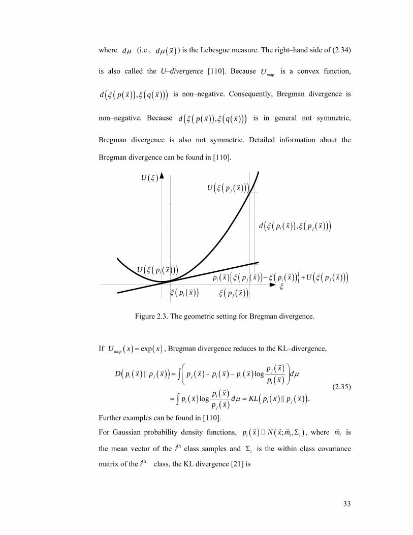
33
where dμ (i.e., ( )d xμ r ) is the Lebesgue measure. The right–hand side of (2.34)
is also called the U–divergence [110]. Because mapU is a convex function,
( )( ) ( )( )( ),d p x q xξ ξr r is non–negative. Consequently, Bregman divergence is
non–negative. Because ( )( ) ( )( )( ),d p x q xξ ξr r is in general not symmetric,
Bregman divergence is also not symmetric. Detailed information about the
Bregman divergence can be found in [110].
( )( )( )iU p xξ r
( )( )ip xξ r ( )( )jp xξ r
( )( )( )jU p xξ r
( )( ) ( )( )( ),i jd p x p xξ ξr r
( ) ( )( ) ( )( ){ } ( )( )( )i j i jp x p x p x U p xξ ξ ξ− +r r r r
ξ
( )U ξ
Figure 2.3. The geometric setting for Bregman divergence.
If ( ) ( )expmapU x x= , Bregman divergence reduces to the KL–divergence,
( ) ( )( ) ( ) ( ) ( ) ( )( )
( ) ( )( ) ( ) ( )( )
|| log
log || .
ji j j i i
i
ii i j
j
p xD p x p x p x p x p x d
p x
p xp x d KL p x p x
p x
μ
μ
⎛ ⎞= − −⎜ ⎟⎜ ⎟
⎝ ⎠
= =
∫
∫
rr r r r r
r
rr r r
r
(2.35)
Further examples can be found in [110].
For Gaussian probability density functions, ( ) ( ); ,i i ip x N x m Σr r r , where imr is
the mean vector of the ith class samples and iΣ is the within class covariance
matrix of the ith class, the KL divergence [21] is
34
( ) ( )( ) ( ) ( )( )
( ) ( )1 1
; ,|| ; , ln
; ,
ln ln tr tr ,
i ii j i i
j j
j i j i j ij
N x mKL p x p x N x m dx
N x m
D− −
Σ= Σ
Σ
= Σ − Σ + Σ Σ + Σ
∫r r
r r r r rr r
(2.36)
where ( ) ( )ij i j i jD m m m m= − ⊗ −r r r r and ( )detΣ Σ .
To simplify the notation we denote the KL divergence between the projected
densities ( )|Tp U x y i=r and ( )|Tp U x y j=r by
( ) ( ) ( )( )|| | || |T TU i jD p p D p U x y i p U x y j= =
r r . (2.37)
General Averaged Divergences Analysis
We replace the arithmetic mean by the generalized mean [48],
( )( )( )
11
1
||i j U i ji j c
m nm n c
q q D p pV U
q qϕ
ϕϕ ≤ ≠ ≤−
≤ ≠ ≤
⎡ ⎤⎢ ⎥
= ⎢ ⎥⎢ ⎥⎣ ⎦
∑∑
, (2.38)
where ( )ϕ ⋅ is a strict monotonic real–valued increasing function defined on
( )0,+∞ ; ( )1ϕ− ⋅ is the inverse function of ( )ϕ ⋅ ; iq is the prior probability of
the ith class (usually, we set i iq n n= or simply set 1iq c= ); ( )||U i jD p p is
defined in (2.37); Lx R∈r where LR is the feature space containing the training
samples; and 'L LU R ×∈ ( 'L L> ) is the projection matrix. The general averaged
divergences function measures the average of all divergences between pairs of
classes in the subspace. We obtain the projection matrix *U by maximizing the
general averaged divergences function ( )V Uϕ over U , for a fixed ( )ϕ ⋅ . The
general optimization algorithm for subspace selection based on (2.38) is given in
Table 2.4. Usually, the concavity of the averaged divergences cannot be
guaranteed. To reduce the effects of local maxima [11], we choose a number of
different initial projection matrices; carry out the separate optimizations; and then
select the best one, which has the maximal value of ( )V Uϕ .
If ( )V Uϕ depends only on the subspace of nR spanned by the columns of U
then U can be replaced by UC where C is a k k× matrix, chosen such that
the columns of UC are orthogonal.
35
On setting ( )x xϕ = , we obtain the arithmetic mean based method for choosing a
subspace,
( )1
1
||* arg max i j U i j
U i j c m nm n c
q q D p pU
q q≤ ≠ ≤≤ ≠ ≤
= ∑ ∑ ( )1
arg max ||i j U i jU i j c
q q D p p≤ ≠ ≤
= ∑ . (2.39)
Table 2.4. General Averaged Divergences Analysis for Subspace Selection
Input: Training samples ;i jxr in LR , where i denotes the ith class (1 i c≤ ≤ ) and j denotes the jth sample in the ith class (1 ij n≤ ≤ ), the dimension 'L( 'L L< ) of the projected subspace, and M is the maximum number of different initial values for the projection matrix.
Output: Optimal linear projection matrix *U in 'L LR × .
1. for 1:m M= {
2. Randomly initialize mtU ( 1t = ), i.e., all entries of 1
mU are random numbers.
3. while ( ) ( )1m mt tV U V Uϕ ϕ ε−− > ( 610ε −= ), do{
4.
Conduct the gradient steepest ascent algorithm3 to maximize the averaged divergences defined in (2.38):
( )1 1m m mt t U tU U V Uϕκ− −← + ⋅∂ . Here, κ , a small value (e.g., 0.0001),
is the learning rate.
5. 1t t← +
6. }//while in line 3
7. }//for in line 1
8. ( )* arg max mt
mU V Uϕ← .
Observation 2.1: LDA maximizes the arithmetic mean of the KL divergences
between all pairs of classes, under the assumption that the Gaussian distributions
( )ip xr for different classes all have the same covariance matrix. The optimal
3 The gradient steepest ascent algorithm can be replaced by other faster optimization methods, such as the conjugate gradient method, to reduce the number of iterations.
36
projection matrix U with respect to LDA can be obtained by maximizing a
particular ( )V Uϕ , i.e.,
( ) ( )( )1
1arg max || arg max tr T T
i j U i j w bU Ui j c
q q D p p U S U U S U−
≤ ≠ ≤
=∑ . (2.40)
Proof: See Appendix.
Example: Decell and Mayekar [29] maximized the weighted arithmetic mean of
all symmetric KL divergences between all pairs of classes in the projected
subspace. The weighting factor of the symmetric KL divergence between the ith
class and the jth class is i jq q , where iq is the prior probability of the ith
class.The symmetric KL divergence is:
( ) ( ) ( )
( ) ( )( )( )( )1 1 1 1
1 1|| || ||2 2
tr tr .
i j i j j i
T
j i i j j i i j i j
SKL p p KL p p KL p p
m m m m− − − −
= +
= Σ Σ +Σ Σ + Σ + Σ − −r r r r
(2.41)
It follows from (2.41) that Decell and Mayekar’s method also maximizes the
arithmetic mean of all KL divergences.
De la Torre and Kanade [28] developed ODA based on the objective function
(2.12) used in [29], but using the iterative majorization to quickly obtain a
solution.
How to Deal with the Multimodal Problem [50]
Up to this point it has been assumed that the samples in a given class are sampled
from a single Gaussian distribution. This assumption often fails in real–world
large data sets, such as those used for multi–view face [84] and gait [176]
recognition, natural image classification [156] or texture classification [133].
To overcome this limitation, each class can be modelled by a GMM. Many
methods for obtaining GMMs have been described in the literature. Examples
include KMeans [30], GMM with expectation–maximization (EM) [30], graph–
cut [131], and spectrum clustering. Unfortunately, these methods are not adaptive,
in that the number of subclusters must be specified, and some of them (e.g., EM
and KMeans) are sensitive to initial values. In our algorithm we use the recently
introduced GMM–EM like algorithm, proposed by Figueiredo and Jain [36],
which is named the GMM–FJ method. The reasons for choosing GMM–FJ are: it
finds the number of subclusters; it is less sensitive to the choice of initial values of
37
parameters than EM; and it avoids the boundary problem4 of the parameter space.
We assume that samples in each class are sampled from a GMM and the
projection matrix U can be obtained by maximizing the general averaged
divergences, which measure the averaged distortion between any pair of
subclusters in different classes, i.e.,
( )( )( )
1 1 11
1 1 1
||i j
i j
k l k li j U i j
i j c k C l C
s tm n
m n c s C t C
q q D p pV U
q qϕ
ϕϕ ≤ ≠ ≤ ≤ ≤ ≤ ≤−
≤ ≠ ≤ ≤ ≤ ≤ ≤
⎡ ⎤⎢ ⎥
= ⎢ ⎥⎢ ⎥⎢ ⎥⎣ ⎦
∑ ∑ ∑
∑ ∑ ∑, (2.42)
where kiq is the prior probability of the kth subcluster of the ith class; k
ip is the
sample density of the samples in the kth subcluster in the ith class; ( )||k lU i jD p p is
the divergence between the kth subcluster in the ith class and the lth subcluster in
the jth class.
4 The means of each class is equal to one of the samples and the covariances are arbitrarily close to singular. For example, we have N samples and we use N Gaussians to model these samples. The mean of each Gaussian is equivalent to a sample and the covariance of each Gaussian is singular.
38
Geometric Mean for Subspace Selection
In LDA and ODA, the arithmetic mean of the divergences is used to find a
suitable subspace into which to project the samples. The main benefit of using the
arithmetic mean in LDA is that the projection matrix can be obtained by the
generalized eigenvalue decomposition. However, LDA is not optimal for
multiclass classification [103] because of the class separation problem defined in
§103. Therefore, it is useful to investigate other choices of ϕ in (2.38) to see if
better results can be obtained.
Criterion 1: Maximization of the Geometric Mean of the Divergences
The log function is a suitable choice for ϕ because it increases the effects of
small divergences and at the same time reduces the effects of large divergences.
On setting ( ) ( )logx xϕ = in (2.38), the generalized geometric mean of the
divergences is obtained. The required subspace *U is given by,
( ) 11
* arg max ||i j
m nm n c
q q
q qU i j
U i j c
U D p p≤ ≠ ≤
≤ ≠ ≤
∑⎡ ⎤= ⎣ ⎦∏ . (2.43)
It follows from the mean inequality that the generalized geometric mean is upper
bounded by the arithmetic mean of the divergences, i.e.,
( ) ( )111
1
|| ||i j
m nm n c
q qi jq q
U i j U i ji j ci j c m n
m n c
q qD p p D p p
q q≤ ≠ ≤≤ ≠ ≤≤ ≠ ≤
≤ ≠ ≤
⎛ ⎞⎜ ⎟∑⎡ ⎤ ≤⎣ ⎦ ⎜ ⎟⎜ ⎟⎝ ⎠
∑∏ ∑. (2.44)
Proof: See Appendix.
Furthermore, (2.43) emphasizes the total volume of all divergences. For example,
in the special case i jq q= for all ,i j ,
( ) ( )11 1
arg max || arg max ||i j
i jm n
m n c
q qq q
q qU i j U i j
U Ui j c i j c
D p p D p p≤ ≠ ≤
≤ ≠ ≤ ≤ ≠ ≤
∑⎡ ⎤ ⎡ ⎤=⎣ ⎦ ⎣ ⎦∏ ∏
( )1
arg max ||U i jU i j c
D p p≤ ≠ ≤
= ∏ . (2.45)
39
Criterion 2: Maximization of the Geometric Mean of the Normalized Divergences
We can further strengthen the effects of small divergences on subspace selection,
by maximizing the geometric mean5 of all normalized divergences6 in the
projected subspace, i.e.,
( )( )
( )1
1
1 1
* arg max || arg max ||c c
U i j U i jU Ui j c i j c
U E p p E p p−
≤ ≠ ≤ ≤ ≠ ≤
⎡ ⎤= =⎢ ⎥
⎣ ⎦∏ ∏ , (2.46)
where the normalized divergence ( )||U i jE p p between the ith class and the jth
class is defined by:
( ) ( )( )
1
||||
||i j U i j
U i jm n U m n
m n c
q q D p pE p p
q q D p p≤ ≠ ≤
=∑
. (2.47)
The intuition behind (2.46) is that the product of normalized divergences is large
when the normalized divergences are similar to each other. Therefore, maximizing
the geometric mean of the normalized divergences will tend to make them as
similar as possible. The effects of the small divergences should then be
emphasized.
Criterion 3: Maximization of the Geometric Mean of all Divergences
Although criterion 2 emphasizes small divergences during optimization, direct use
of the criterion is not desirable for subspace selection. This is because
experiments in §233066540 show that there exists U for which all divergences
become small, but all normalized divergences are comparable in size. In such
case, the projection matrix U is not suitable for classification, because several
classes may be severely overlapped.
To reduce this problem, we combine criterion 2 with criterion 1 into a new one.
The new criterion maximizes the linear combination of: 1) the log of the
5 In (2.46), we use the geometric mean but not the generalized geometric mean because the weights (the prior probabilities iq ) are moved to the normalized divergences as shown in (2.47). In this form, the calculations are simplified. 6 The sum of all normalized divergences is one.
40
geometric mean of the divergences and 2) the log of the geometric mean of
normalized divergences. This criterion is named the Maximization of the
Geometric Mean of all Divergences, or briefly MGMD,
( )( )
( ) ( )
( ) ( )
1
11
1
1
1 1
log ||* arg max
1 log ||
arg max log || log || ,
i j
m nm n c
c c
U i ji j c
q qUq q
U i ji j c
U i j i j U i jU i j c i j c
E p pU
D p p
D p p q q D p p
α
α
η
≤ ≠ ≤
−
≤ ≠ ≤
≤ ≠ ≤
≤ ≠ ≤ ≤ ≠ ≤
⎧ ⎫⎡ ⎤⎪ ⎪⎢ ⎥⎪ ⎪⎪ ⎪⎣ ⎦= ⎨ ⎬
⎪ ⎪∑⎡ ⎤+ −⎪ ⎪⎣ ⎦⎪ ⎪⎩ ⎭
⎧ ⎫⎛ ⎞⎪ ⎪= −⎨ ⎬⎜ ⎟⎪ ⎪⎝ ⎠⎩ ⎭
∏
∏
∑ ∑
(2.48)
where 0 1α< < is the linear combination coefficient to integrate the criterion 1
with 2; and ( )
( )( )1
1
1
1 1
m nm n c
m nm n c
c c q q
c c q q
αη
α α≤ ≠ ≤
≤ ≠ ≤
−=
− − +
∑∑
. The supremum of η is ( )1c c −
and the infimum of η is 0. When 0α = (or 0η = ), (2.48) reduces to (2.43);
and when 1α = (or ( )1c cη = − ), (2.48) reduces to (2.46). The rational of the
combination coefficient α trades off the geometric mean of divergences of
different pairs of classes against the geometric mean of normalized divergences of
different pairs of classes. The first part emphasizes the total volume of all
divergences; increases effects of small divergences; and reduces effects of large
divergences. The second part further strengthens the effects of small divergences
and weakens theeffects of large divergences. Therefore, by tuning the parameter
α , we can balance the impacts of selected subspace on the total volume of all
divergences, the impacts of large divergences, and the impacts of small ones.
Deduction 2.1: See Appendix.
Based on (2.48) and (2.42), we directly extend MGMD to the multimodal case, as
the Multimodal extension of the Maximization of the Geometric Mean of all
Divergences (M–MGMD),
( )
( )
1 1 1
1 1 1
log ||
* arg maxlog ||
i j
i j
k lU i j
i j c k C l C
U k l k li j U i j
i j c k C l C
D p p
Uq q D p pη
≤ ≠ ≤ ≤ ≤ ≤ ≤
≤ ≠ ≤ ≤ ≤ ≤ ≤
⎧ ⎫⎪ ⎪⎪ ⎪= ⎨ ⎬⎛ ⎞⎪ ⎪− ⎜ ⎟⎜ ⎟⎪ ⎪⎝ ⎠⎩ ⎭
∑ ∑ ∑
∑ ∑ ∑. (2.49)
In the next Section, we discuss subspace selection based on the choice of the KL
divergence in (2.48) and (2.49).
41
Kullback–Leibler Divergence based Subspace Selection
In the last Section, we developed a framework MGMD/M–MGMD for subspace
selection based on the geometric mean of divergences and normalized
divergences. In this Section, we combine the KL divergence with MGMD/M–
MGMD as an example for practical applications. The multimodal problem [50] is
carefully studied and finally we kernelize the proposed subspace selection
method. Experimental studies are given in §50, §50, and §50.
MGMD and KL Divergence for Subspace Selection
By combining the KL divergence defined in (2.36) and MGMD defined in (2.48),
we obtain the Maximization of the Geometric Mean of all KL Divergences
(MGMKLD),
( )* arg maxU
U L U= , (2.50)
where ( )L U is defined by
( ) ( ) ( )1 1
log || log ||U i j i j U i ji j c i j c
L U KL p p q q KL p pη≤ ≠ ≤ ≤ ≠ ≤
⎛ ⎞= − ⎜ ⎟
⎝ ⎠∑ ∑ , (2.51)
and ( )||U i jKL p p is the KL divergence between the ith class and the jth class in
the projected subspace,
( )
( ) ( )( ) ( )( )1 1
1|| log log2
tr tr
T TU i j j i
T T T Tj i j ij
KL p p U U U U
U U U U U U U D U− −
= Σ − Σ
+ Σ Σ + Σ (2.52)
To better understand MGMKLD, we need to define the Stiefel manifold and the
Grassmann manifold.
Definition 2.2: The Stiefel manifold [10] ( ),St n r for n r≥ is defined as a set
of all n r× matrices with orthonormal columns, i.e.,
( , ) { : }n r TrSt n r U R U U I×= ∈ = . ( ),St n r is a sub–manifold of n rR × of real
dimension 22n r r× − . Two elements 1U and 2U in ( ),St n r are said to be
equivalent if their columns span the same subspace, i.e., 1 2U U Q= for some
orthogonal matrix r rQ R ×∈ .
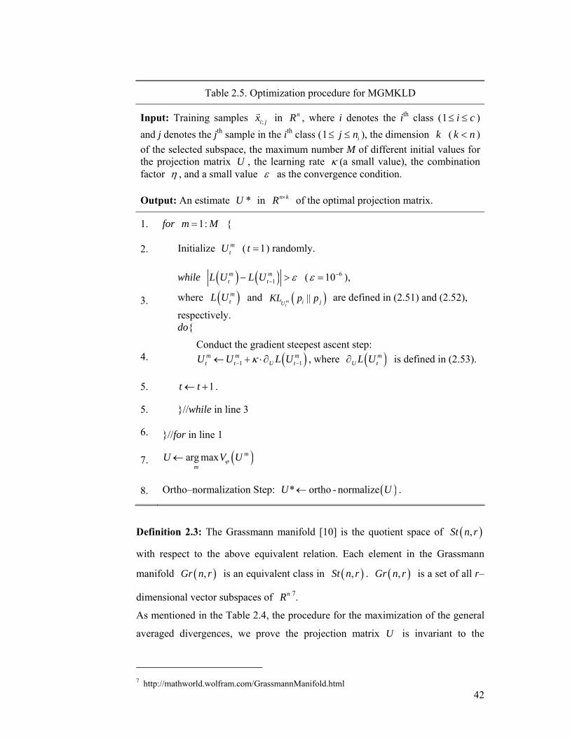
42
Table 2.5. Optimization procedure for MGMKLD
Input: Training samples ;i jxr in nR , where i denotes the ith class (1 i c≤ ≤ ) and j denotes the jth sample in the ith class (1 ij n≤ ≤ ), the dimension k ( k n< ) of the selected subspace, the maximum number M of different initial values for the projection matrix U , the learning rate κ (a small value), the combination factor η , and a small value ε as the convergence condition.
Output: An estimate *U in n kR × of the optimal projection matrix.
1. for 1:m M= {
2. Initialize mtU ( 1t = ) randomly.
3.
while ( ) ( )1m mt tL U L U ε−− > ( 610ε −= ),
where ( )mtL U and ( )||m
ti jU
KL p p are defined in (2.51) and (2.52),
respectively. do{
4. Conduct the gradient steepest ascent step:
( )1 1m m mt t U tU U L Uκ− −← + ⋅∂ , where ( )m
U tL U∂ is defined in (2.53).
5. 1t t← + .
5. }//while in line 3
6. }//for in line 1
7. ( )arg max m
mU V Uϕ←
8. Ortho–normalization Step: ( )* ortho - normalizeU U← .
Definition 2.3: The Grassmann manifold [10] is the quotient space of ( ),St n r
with respect to the above equivalent relation. Each element in the Grassmann
manifold ( ),Gr n r is an equivalent class in ( ),St n r . ( ),Gr n r is a set of all r–
dimensional vector subspaces of nR 7.
As mentioned in the Table 2.4, the procedure for the maximization of the general
averaged divergences, we prove the projection matrix U is invariant to the
7 http://mathworld.wolfram.com/GrassmannManifold.html
43
ortho–normalization operator for ( )L U , i.e., U stays in the Grassmann
manifold. In other words, ( )L U will depend only on the subspace defined by
U .
Claim 2.1: The ortho–normalization operation does not change the value of the
objective function ( )L U of MGMKLD defined in (2.51).
Proof: See Appendix.
To obtain the optimization procedure for MGMKLD based on Table 2.4, we need
the first order derivative of ( )L U ,
( )( ) ( )
( ) ( )
1
1
1
1 1
|| ||
|| || ,
U
U i j U U i ji j c
m n U m n i j U U i jm n c i j c
L U
KL p p KL p p
q q KL p p q q KL p pη
−
≤ ≠ ≤
−
≤ ≠ ≤ ≤ ≠ ≤
∂
= ∂
⎛ ⎞⎛ ⎞− ∂⎜ ⎟⎜ ⎟⎝ ⎠ ⎝ ⎠
∑
∑ ∑
(2.53)
where the first order derivative of ( )||U i jKL p p is given by
( )( ) ( ) ( ) ( )( ) ( ) ( )
1 1 1
1 1
||
.
U U i j
T T Tj j i i i ij j
T T Tj j i ij j
KL p p
U U U U U U D U U U
U U U U D U U U
− − −
− −
∂
= Σ −Σ Σ + Σ + Σ
−Σ Σ Σ + Σ
Σ (2.54)
Multimodal Extension of MGMKLD
In many situations, the distribution of each class is not Guassian. It is reasonable
to use GMMs to fit each class. The advantages of introducing GMM to
discriminative subspace selection are described in §0. In this Section, we combine
GMM with MGMKLD as the multimodal extension of MGMKLD (M–
MGMKLD). The combination, M–MGMKLD, is obtained from (2.36) and (2.49),
as
( )* arg max GMMU
U L U=
( )
( )
1 1 1
1 1 1
arg max log ||
log || .
i j
i j
k li j
U i j c k C l C
k l k li j U i j
i j c k C l C
KLU p p
q q KL p pη
≤ ≠ ≤ ≤ ≤ ≤ ≤
≤ ≠ ≤ ≤ ≤ ≤ ≤
⎡ ⎤= ⎣ ⎦
⎡ ⎤⎡ ⎤− ⎢ ⎥⎣ ⎦⎢ ⎥⎣ ⎦
∑ ∑ ∑
∑ ∑ ∑
W
(2.55)
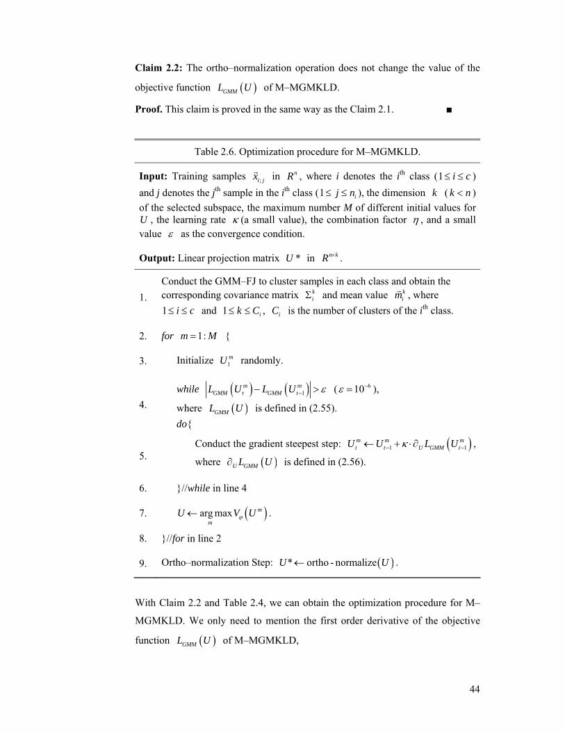
44
Claim 2.2: The ortho–normalization operation does not change the value of the
objective function ( )GMML U of M–MGMKLD.
Proof. This claim is proved in the same way as the Claim 2.1. ■
Table 2.6. Optimization procedure for M–MGMKLD.
Input: Training samples ;i jxr in nR , where i denotes the ith class (1 i c≤ ≤ ) and j denotes the jth sample in the ith class (1 ij n≤ ≤ ), the dimension k ( k n< ) of the selected subspace, the maximum number M of different initial values forU , the learning rate κ (a small value), the combination factor η , and a small value ε as the convergence condition.
Output: Linear projection matrix *U in n kR × .
1. Conduct the GMM–FJ to cluster samples in each class and obtain the corresponding covariance matrix k
iΣ and mean value kimr , where
1 i c≤ ≤ and 1 ik C≤ ≤ , iC is the number of clusters of the ith class.
2. for 1:m M= {
3. Initialize 1mU randomly.
4. while ( ) ( )1
m mGMM t GMM tL U L U ε−− > ( 610ε −= ),
where ( )GMML U is defined in (2.55). do{
5. Conduct the gradient steepest step: ( )1 1
m m mt t U GMM tU U L Uκ− −← + ⋅∂ ,
where ( )U GMML U∂ is defined in (2.56).
6. }//while in line 4
7. ( )arg max m
mU V Uϕ← .
8. }//for in line 2
9. Ortho–normalization Step: ( )* ortho - normalizeU U← .
With Claim 2.2 and Table 2.4, we can obtain the optimization procedure for M–
MGMKLD. We only need to mention the first order derivative of the objective
function ( )GMML U of M–MGMKLD,

45
( ) ( ) ( )
( )
1
1 1 1
1
1 1 1
|| ||
||
i j
i j
k l k lU GMM U i j U U i j
i j c k C l C
s t s tm n U m n
m n c s C t C
L U KL p p KL p p
q q KL p pη
−
≤ ≠ ≤ ≤ ≤ ≤ ≤
−
≤ ≠ ≤ ≤ ≤ ≤ ≤
∂ = ∂
⎛ ⎞− ⎜ ⎟⎜ ⎟
⎝ ⎠
∑ ∑ ∑
∑ ∑ ∑
( )1 1 1
|| .i j
k l k li j U U i j
i j c k C l Cq q KL p p
≤ ≠ ≤ ≤ ≤ ≤ ≤
⎛ ⎞∂⎜ ⎟⎜ ⎟
⎝ ⎠∑ ∑ ∑
(2.56)
By incorporating the merits of GMM–FJ and the proposed MGMKLD model, the
new method has the following benefits:
1. Experiments show that the new method reduces the class separation
problem;
2. The new method inherits the merits of GMM–FJ. In detail, it determines
the number of subclusters in each class automatically; it is less sensitive to
the choice of initial values of the parameters than EM; and it avoids the
boundary problem of the parameter space;
3. The new method is capable of obtaining the projection orthogonal matrix,
i.e., ( )GMML U depends only on the subspace defined by U .
Kernel Extension of MGMKLD
In this part, we study the kernel extension of MGMKLD. Because of the success
of the kernel method [129][109] in pattern classification, MGMKLD will be
generalized from the low dimensional original Hilbert space to the higher
dimensional Hilbert space. The generalized version is named the kernel
MGMKLD (KMGMKLD).
To utilize the kernel dot product trick [129][109] for MGMKLD, we need to have
the Lemma 2.1. Denote ⊕ as the direct sum.
Lemma 2.1: If U is a solution to MGMKLD and x xU U U ⊥= ⊕ , then xU is a
solution to MGMKLD. We have ( ) ( )xL U L U= . Here, the column space of xU
is spanned by the samples { } 1; 1| ij n
i j i cx ≤ ≤≤ ≤
r and the column space of xU ⊥ is the
orthogonal complement of the column space of xU .
Proof: See Appendix.
From Lemma 2.1, we know that the orthogonal complement component xU ⊥
( xU U= ) does not affect the objective function ( )L U of MGMKLD defined in
46
(2.51). Consequently, we can set 0xU ⊥ = , i.e., the column space of U is
spanned by the samples { } 1; 1| ij n
i j i cx ≤ ≤≤ ≤
r . Based on Lemma 2.1, the kernel trick can be
utilized to implement the kernel extension of MGMKLD, because ( )L U defined
in (2.51) can be fully expressed in terms of inner products with the samples
{ } 1; 1| ij n
i j i cx ≤ ≤≤ ≤
r only. Without this lemma, the kernelization of MGMKLD cannot be
implemented.
Herein, there is a mapping rule : L HR Rφ a to map MGMKLD to a higher–
dimensional space [109][104][129]. The samples xr , which are modelled by
( ),i iN m Σr , are mapped as
( ) ( ) ( )( ); ; ~ ,i j i j i ix x N mφ φ φ→ Σr r r (2.57)
( ); ;1
1 in
i i jji
m xnφ φ
=
= ∑r r (2.58)
( )( ) ( )( ); ; ; ; ;
T
i i j i i j iE x m x mφ φ φφ φ⎡ ⎤Σ = − −⎢ ⎥⎣ ⎦r r r r (2.59)
where ;imφr is the mean vector of the ith class in HR and ;iφΣ is the covariance
matrix of the ith class in HR .
Based on Lemma 2.1, we can choose the projection matrix in HR as
( ) ( ); ; ; *1 1
inc
i j i j i j n FF ni jU x xφ α φ φ ××
= =
⎡ ⎤= = Λ⎣ ⎦∑∑ r r , (2.60)
where ;i jα is the linear combination coefficient to combine the training samples
( );i jxφ r in HR .
This means each column of Uφ is a linear combination of all ( );i jxφ r by
varying i and j from all classes and samples in each class.
Therefore, the KL divergence ( )( ) ( )( )( )||U i jKL p x p xφ φr r in the feature space is
( )( ) ( )( )( )
( ) ( )( )( ); ;
1
; ; ;
||
log log12 tr
U i j
T Tj i
T Tj j ij
KL p x p x
U U U U
U U U D U
φ
φ φ φ φ φ φ
φ φ φ φ φ φ φ
φ φ
−
⎛ ⎞Σ − Σ⎜ ⎟= ⎜ ⎟+ Σ Σ +⎜ ⎟⎝ ⎠
r r
. (2.61)
Therefore, (2.51) becomes
47
( ) ( )( ) ( )( )( )
( )( ) ( )( )( )1
1
log ||
log ||
U i ji j c
m n U m nm n c
L U KL p x p x
q q KL p x p x
φ
φ
φ φ φ
η φ φ
≤ ≠ ≤
≤ ≠ ≤
⎡ ⎤= ⎣ ⎦
⎡ ⎤− ⎢ ⎥⎣ ⎦
∑
∑
r r
r r. (2.62)
The variable ijD becomes
( ) ( ) ( ) ( ); ; ; ; ;1 1 1 1
1 1 1 1j ji iTn nn n
ij i k i l i k i lk l k li j i j
D x x x xn n n nφ φ φ φ φ
= = = =
⎛ ⎞⎛ ⎞= − −⎜ ⎟⎜ ⎟⎜ ⎟⎜ ⎟⎝ ⎠⎝ ⎠∑ ∑ ∑ ∑r r r r . (2.63)
To obtain the kernel Gram matrix [129] based representation in (2.61), we need to
reformulate ( ) ;T
iU U Uφ φ φΣ by the kernel dot product trick8 as:
;
' , , , , '1 1 11 1
i i i i i i i i i i
Ti
TT Tn H C C C C C C C C C C n H
i i i
U U
K I I Kn n n
φ φ φ
× ×
Σ
⎛ ⎞⎛ ⎞= Λ − − Λ⎜ ⎟⎜ ⎟
⎝ ⎠⎝ ⎠
, (2.64)
Deduction 2.2: See Appendix.
where .; jK is the ( )1
1
thikk
n j−
=+∑ column of the kernel Gram matrix
( ) ( ); ;
T
i j i jF n F nK x xφ φ
× ×⎡ ⎤ ⎡ ⎤= ⎣ ⎦ ⎣ ⎦
r r ( ); ;,i j i jk x x⎡ ⎤= ⎣ ⎦r r , ( ); ;,i j i jk x xr r is the kernel function
[129], ,,
C Ci i
i iC CI R∈ is the identity matrix, ,,1 i i
i i
C CC C R∈ is the unit matrix,
.; 1i iC j j n
K K≤ ≤
⎡ ⎤= ⎣ ⎦ is composed of the columns in the kernel Gram matrix from the
( )1
11
thikk
n−
=+∑ column to the ( )1
thikk
n=∑ column; 'n H×Λ is the projection
matrix in HR and 'H is the number of selected features in HR .
With the kernel dot product trick we can transform ;T
ijU D Uφ φ φ into
;
' '1 1 1 11 1 1 1
i i j j i i j j
Tij
T
Tn H C C C C C C C C n H
i j i j
U D U
K K K Kn n n n
φ φ φ
× ×
⎛ ⎞⎛ ⎞= Λ − − Λ⎜ ⎟⎜ ⎟⎜ ⎟⎜ ⎟
⎝ ⎠⎝ ⎠
. (2.65)
Deduction 2.3: See Appendix.
Therefore, we can reformulate (2.61) as:
8 The kernel dot product trick is used to transform a linear algorithm (for classification, subspace selection, regression, and etc.) to a non–linear one by mapping the original samples in a low dimensional space into a higher dimensional space. Based on this mapping, the linear algorithm in the new space is equivalent to non–linear algorithm in the original space. The trick transforms a linear algorithm by replacing the dot product between two vectors with a kernel function.
48
( )
( )
' ' ' '
1
' ' ' , , '
1
' ' ' '
1 1log log
1 1tr2
1 1tr
j j i i
j j i j i j
j j i i
ij
T T T Tn H C C n H n H C C n H
j i
T T T Tn H C C n H n H C C C C n H
j
T T T Tn H C C n H n H C C n H
j i
KL U
K K K Kn n
K K L Ln
K K K Kn n
φ
× × × ×
−
× × × ×
−
× × × ×
⎛⎜ Λ Λ − Λ Λ⎜⎜⎜ ⎛ ⎞⎛ ⎞⎜ ⎜ ⎟= + Λ Λ Λ Λ⎜ ⎟⎜ ⎟⎜ ⎟⎝ ⎠⎝ ⎠
⎛ ⎞⎛ ⎞ ⎛ ⎞⎜ ⎟+ Λ Λ Λ Λ⎜ ⎟ ⎜ ⎟⎜ ⎟⎜ ⎟⎝ ⎠⎝ ⎠⎝ ⎠⎝
⎞⎟⎟⎟⎟⎟
⎜ ⎟⎜ ⎟⎜ ⎟⎜ ⎟⎜ ⎟⎜ ⎟
⎠
, (2.66)
where jCK and ,i jC CL are defined by:
, ,1 1
j j j j j jC C C C C Cj
K K In
⎛ ⎞= −⎜ ⎟⎜ ⎟
⎝ ⎠ (2.67)
,1 11 1
i j i i j jC C C C C Ci j
L K Kn n
⎛ ⎞= −⎜ ⎟⎜ ⎟⎝ ⎠
. (2.68)
For a given sample zr , the corresponding feature ( )TU zφ φr in the higher
dimensional space is given by:
( ) ( ) ( ) ( )' ; ' ; ,T TT T T
n H i j n H i jH n H nU z x z k x zφ φ φ φ× ×× ×
⎡ ⎤ ⎡ ⎤= Λ = Λ⎣ ⎦ ⎣ ⎦r rr r r , (2.69)
where ( ); ,i jk x zr r is the kernel function with entries ;i jxr and zr . There are many
typical kernel functions that could be used here, e.g., the Gaussian radial basis
kernels ( ( ) ( )( )2 2, exp 2k x x x x σ′ ′= − −r r r r ), the homogeneous polynomial kernels
( ( ), , dk x x x x′ ′=r r r r ), the inhomogeneous polynomial kernels ( ( ),k x x′ =
r r
( ),d
x x c′ +r r ), and the sigmoid kernels ( ( ) ( ), tanh ,k x x x xκ ϑ′ ′= − +
r r r r ). The
homogeneous polynomial kernels and the Gaussian radial basis kernels are widely
used in pattern classification. The homogeneous polynomial kernels are invariant
under orthogonal transformations. Liu [87] empiricially demonstrated that the
fractional powers in the homogeneous polynomial kernels perform better than
integral powers. The radial basis kernels can be written as ( ) ( )( ), ,k x x f d x x′ ′=r r r r ,
where f is a function on R+ and d is a metric function. In Gaussian radial
basis kenrles, f is an exponential function and d is the Euclidean metric. In
different applications, we can choose different f and d through the cross–
validation to achieve reasonable performances.

49
Theorem 2.1: MGMKLD followed by KPCA is equal to KMGMKLD.
Proof: See Appendix.
Theorem 2.2: M–MGMKLD followed by KPCA is equal to the multimodal
extension of KMGMKLD, or briefly M–KMGMKLD.
Proof. The result follows from the Theorem 2.1. ■
In the Theorem 2.1, we show that kernel principal component analysis (KPCA)
following MGMKLD yields kernel MGMKLD. Based on this theorem,
KMGMKLD is equivalent to first preprocessing the data using KPCA and then
applying orthogonal MGMKLD to the preprocessed data.
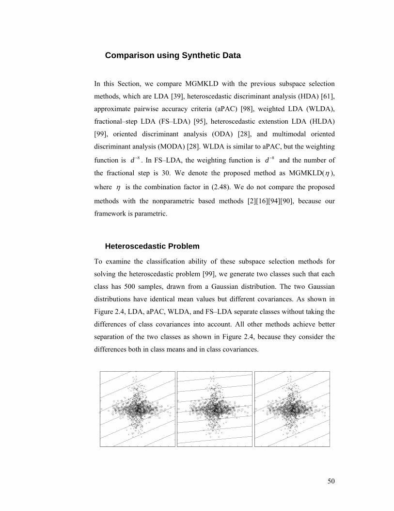
50
Comparison using Synthetic Data
In this Section, we compare MGMKLD with the previous subspace selection
methods, which are LDA [39], heteroscedastic discriminant analysis (HDA) [61],
approximate pairwise accuracy criteria (aPAC) [98], weighted LDA (WLDA),
fractional–step LDA (FS–LDA) [95], heteroscedastic extenstion LDA (HLDA)
[99], oriented discriminant analysis (ODA) [28], and multimodal oriented
discriminant analysis (MODA) [28]. WLDA is similar to aPAC, but the weighting
function is 8d − . In FS–LDA, the weighting function is 8d − and the number of
the fractional step is 30. We denote the proposed method as MGMKLD(η ),
where η is the combination factor in (2.48). We do not compare the proposed
methods with the nonparametric based methods [2][16][94][90], because our
framework is parametric.
Heteroscedastic Problem
To examine the classification ability of these subspace selection methods for
solving the heteroscedastic problem [99], we generate two classes such that each
class has 500 samples, drawn from a Gaussian distribution. The two Gaussian
distributions have identical mean values but different covariances. As shown in
Figure 2.4, LDA, aPAC, WLDA, and FS–LDA separate classes without taking the
differences of class covariances into account. All other methods achieve better
separation of the two classes as shown in Figure 2.4, because they consider the
differences both in class means and in class covariances.
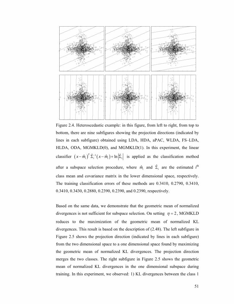
51
Figure 2.4. Heteroscedastic example: in this figure, from left to right, from top to
bottom, there are nine subfigures showing the projection directions (indicated by
lines in each subfigure) obtained using LDA, HDA, aPAC, WLDA, FS–LDA,
HLDA, ODA, MGMKLD(0), and MGMKLD(1). In this experiment, the linear
classifier ( ) ( )1ˆ ˆˆ ˆ lnTi i i ix m x m−− Σ − + Σ is applied as the classification method
after a subspace selection procedure, where ˆ im and ˆiΣ are the estimated ith
class mean and covariance matrix in the lower dimensional space, respectively.
The training classification errors of these methods are 0.3410, 0.2790, 0.3410,
0.3410, 0.3430, 0.2880, 0.2390, 0.2390, and 0.2390, respectively.
Based on the same data, we demonstrate that the geometric mean of normalized
divergences is not sufficient for subspace selection. On setting 2η = , MGMKLD
reduces to the maximization of the geometric mean of normalized KL
divergences. This result is based on the description of (2.48). The left subfigure in
Figure 2.5 shows the projection direction (indicated by lines in each subfigure)
from the two dimensional space to a one dimensional space found by maximizing
the geometric mean of normalized KL divergences. The projection direction
merges the two classes. The right subfigure in Figure 2.5 shows the geometric
mean of normalized KL divergences in the one dimensional subspace during
training. In this experiment, we observed: 1) KL divergences between the class 1
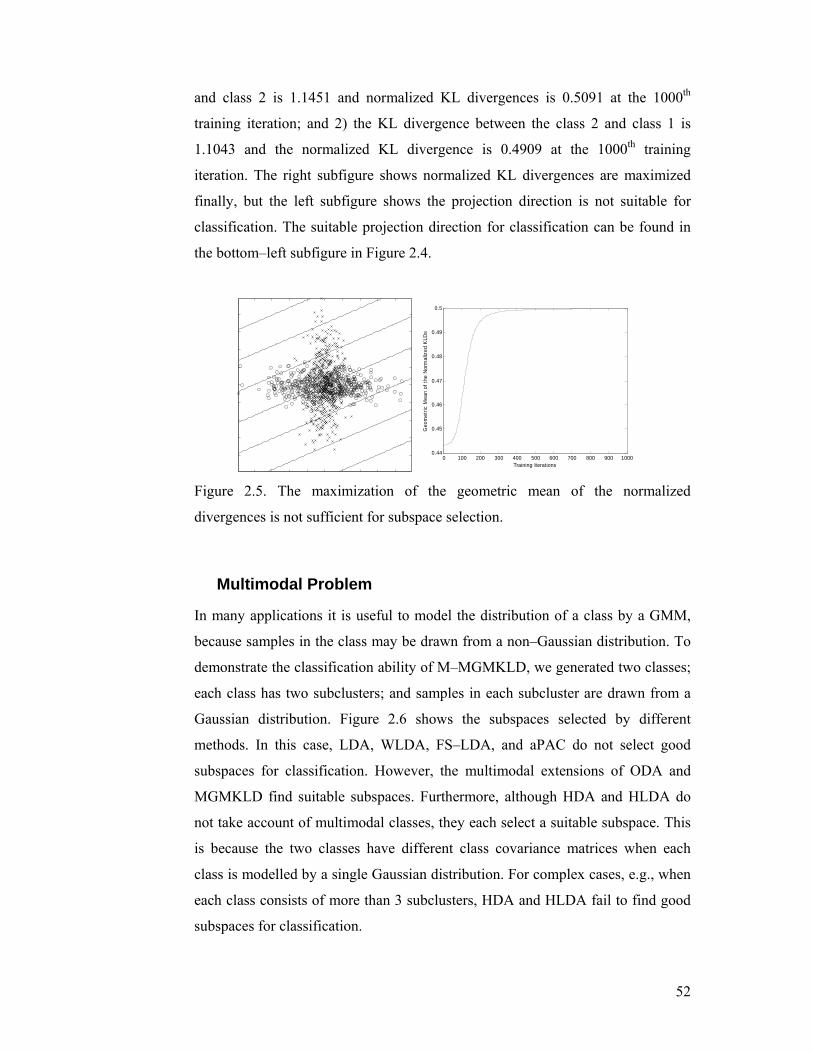
52
and class 2 is 1.1451 and normalized KL divergences is 0.5091 at the 1000th
training iteration; and 2) the KL divergence between the class 2 and class 1 is
1.1043 and the normalized KL divergence is 0.4909 at the 1000th training
iteration. The right subfigure shows normalized KL divergences are maximized
finally, but the left subfigure shows the projection direction is not suitable for
classification. The suitable projection direction for classification can be found in
the bottom–left subfigure in Figure 2.4.
0 100 200 300 400 500 600 700 800 900 10000.44
0.45
0.46
0.47
0.48
0.49
0.5
Training Iterations
Geo
met
ric M
ean
of th
e N
orm
aliz
ed K
LDs
Figure 2.5. The maximization of the geometric mean of the normalized
divergences is not sufficient for subspace selection.
Multimodal Problem
In many applications it is useful to model the distribution of a class by a GMM,
because samples in the class may be drawn from a non–Gaussian distribution. To
demonstrate the classification ability of M–MGMKLD, we generated two classes;
each class has two subclusters; and samples in each subcluster are drawn from a
Gaussian distribution. Figure 2.6 shows the subspaces selected by different
methods. In this case, LDA, WLDA, FS–LDA, and aPAC do not select good
subspaces for classification. However, the multimodal extensions of ODA and
MGMKLD find suitable subspaces. Furthermore, although HDA and HLDA do
not take account of multimodal classes, they each select a suitable subspace. This
is because the two classes have different class covariance matrices when each
class is modelled by a single Gaussian distribution. For complex cases, e.g., when
each class consists of more than 3 subclusters, HDA and HLDA fail to find good
subspaces for classification.
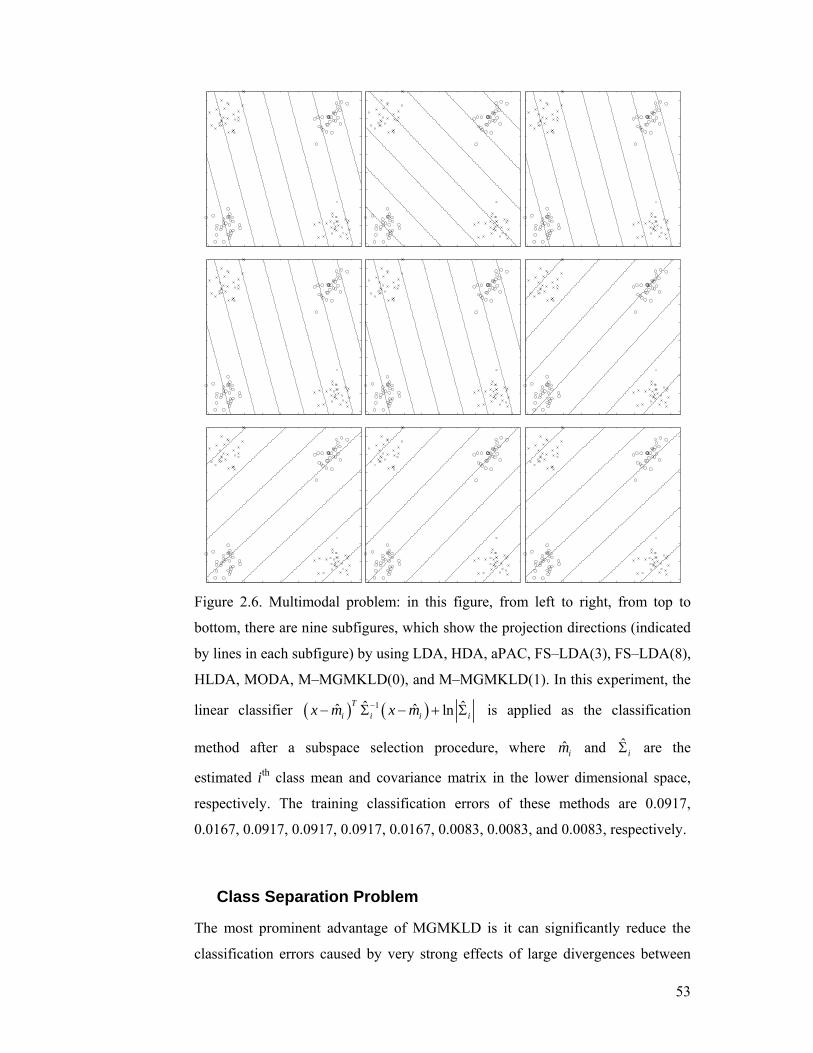
53
Figure 2.6. Multimodal problem: in this figure, from left to right, from top to
bottom, there are nine subfigures, which show the projection directions (indicated
by lines in each subfigure) by using LDA, HDA, aPAC, FS–LDA(3), FS–LDA(8),
HLDA, MODA, M–MGMKLD(0), and M–MGMKLD(1). In this experiment, the
linear classifier ( ) ( )1ˆ ˆˆ ˆ lnTi i i ix m x m−− Σ − + Σ is applied as the classification
method after a subspace selection procedure, where ˆ im and ˆiΣ are the
estimated ith class mean and covariance matrix in the lower dimensional space,
respectively. The training classification errors of these methods are 0.0917,
0.0167, 0.0917, 0.0917, 0.0917, 0.0167, 0.0083, 0.0083, and 0.0083, respectively.
Class Separation Problem
The most prominent advantage of MGMKLD is it can significantly reduce the
classification errors caused by very strong effects of large divergences between
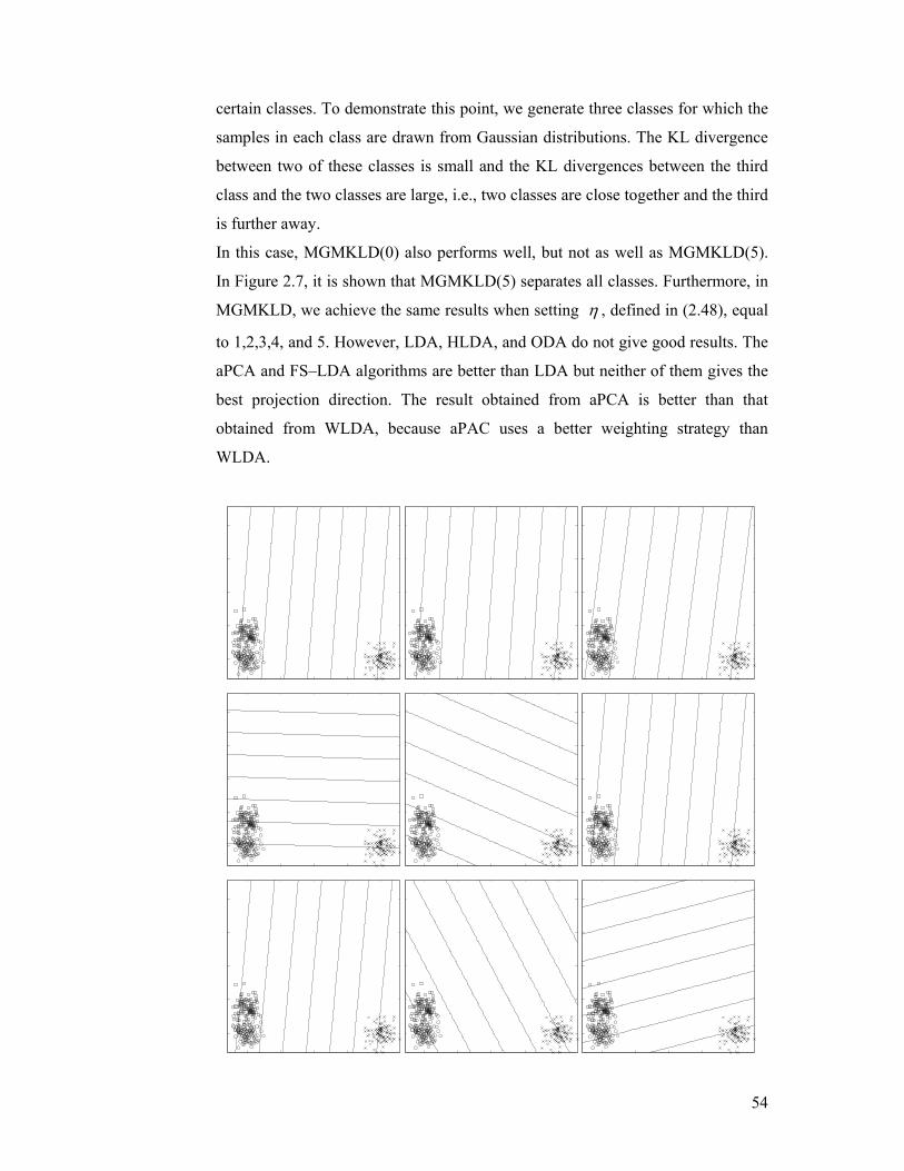
54
certain classes. To demonstrate this point, we generate three classes for which the
samples in each class are drawn from Gaussian distributions. The KL divergence
between two of these classes is small and the KL divergences between the third
class and the two classes are large, i.e., two classes are close together and the third
is further away.
In this case, MGMKLD(0) also performs well, but not as well as MGMKLD(5).
In Figure 2.7, it is shown that MGMKLD(5) separates all classes. Furthermore, in
MGMKLD, we achieve the same results when setting η , defined in (2.48), equal
to 1,2,3,4, and 5. However, LDA, HLDA, and ODA do not give good results. The
aPCA and FS–LDA algorithms are better than LDA but neither of them gives the
best projection direction. The result obtained from aPCA is better than that
obtained from WLDA, because aPAC uses a better weighting strategy than
WLDA.
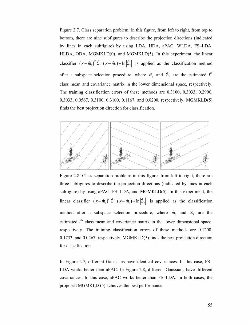
55
Figure 2.7. Class separation problem: in this figure, from left to right, from top to
bottom, there are nine subfigures to describe the projection directions (indicated
by lines in each subfigure) by using LDA, HDA, aPAC, WLDA, FS–LDA,
HLDA, ODA, MGMKLD(0), and MGMKLD(5). In this experiment, the linear
classifier ( ) ( )1ˆ ˆˆ ˆ lnTi i i ix m x m−− Σ − + Σ is applied as the classification method
after a subspace selection procedure, where ˆ im and ˆiΣ are the estimated ith
class mean and covariance matrix in the lower dimensional space, respectively.
The training classification errors of these methods are 0.3100, 0.3033, 0.2900,
0.3033, 0.0567, 0.3100, 0.3100, 0.1167, and 0.0200, respectively. MGMKLD(5)
finds the best projection direction for classification.
Figure 2.8. Class separation problem: in this figure, from left to right, there are
three subfigures to describe the projection directions (indicated by lines in each
subfigure) by using aPAC, FS–LDA, and MGMKLD(5). In this experiment, the
linear classifier ( ) ( )1ˆ ˆˆ ˆ lnTi i i ix m x m−− Σ − + Σ is applied as the classification
method after a subspace selection procedure, where ˆ im and ˆiΣ are the
estimated ith class mean and covariance matrix in the lower dimensional space,
respectively. The training classification errors of these methods are 0.1200,
0.1733, and 0.0267, respectively. MGMKLD(5) finds the best projection direction
for classification.
In Figure 2.7, different Gaussians have identical covariances. In this case, FS–
LDA works better than aPAC. In Figure 2.8, different Gaussians have different
covariances. In this case, aPAC works better than FS–LDA. In both cases, the
proposed MGMKLD (5) achieves the best performance.
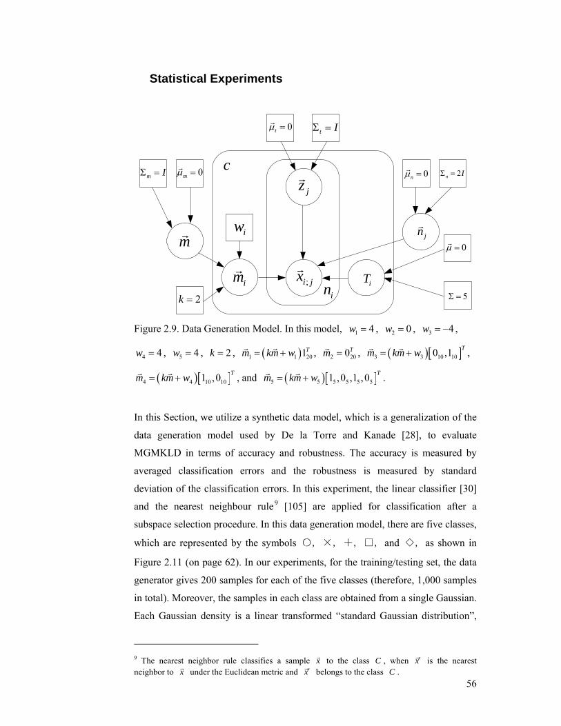
56
Statistical Experiments
jzr
iTimr
jnr
;i jxr
in
c
0tμ =r
t IΣ =
0nμ =r 2n IΣ =
iw
2k =
mr
0mμ =r
m IΣ =
0μ =r
5Σ =
Figure 2.9. Data Generation Model. In this model, 1 4w = , 2 0w = , 3 4w = − ,
4 4w = , 5 4w = , 2k = , ( )1 1 201Tm km w= +r r , 2 200Tm =
r , ( )[ ]3 3 10 100 ,1 Tm km w= +r r ,
( )[ ]4 4 10 101 ,0 Tm km w= +r r , and ( )[ ]5 5 5 5 5 51 ,0 ,1 ,0 Tm km w= +
r r .
In this Section, we utilize a synthetic data model, which is a generalization of the
data generation model used by De la Torre and Kanade [28], to evaluate
MGMKLD in terms of accuracy and robustness. The accuracy is measured by
averaged classification errors and the robustness is measured by standard
deviation of the classification errors. In this experiment, the linear classifier [30]
and the nearest neighbour rule9 [105] are applied for classification after a
subspace selection procedure. In this data generation model, there are five classes,
which are represented by the symbols ○, ×, +, □, and ◇, as shown in
Figure 2.11 (on page 62). In our experiments, for the training/testing set, the data
generator gives 200 samples for each of the five classes (therefore, 1,000 samples
in total). Moreover, the samples in each class are obtained from a single Gaussian.
Each Gaussian density is a linear transformed “standard Gaussian distribution”,
9 The nearest neighbor rule classifies a sample xr to the class C , when x′r is the nearest neighbor to xr under the Euclidean metric and x′r belongs to the class C .
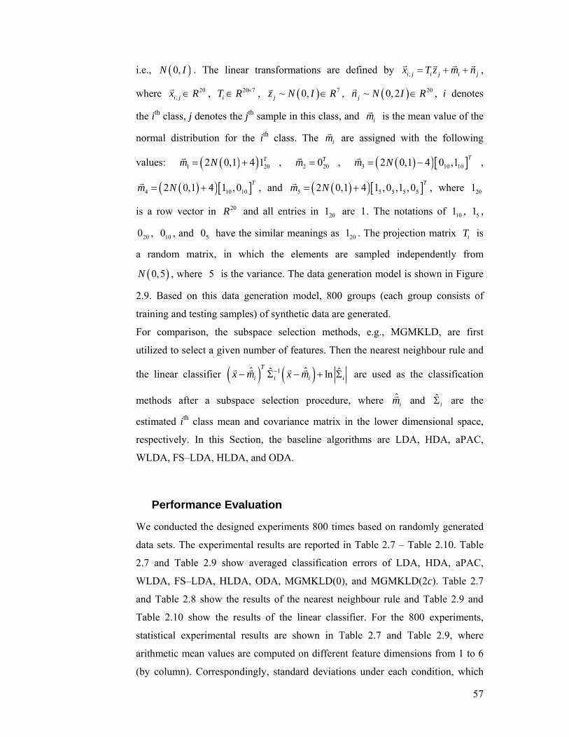
57
i.e., ( )0,N I . The linear transformations are defined by ;i j i j i jx T z m n= + +r r rr ,
where 20;i jx R∈r , 20 7
iT R ×∈ , ( ) 7~ 0,jz N I R∈r , ( ) 20~ 0,2jn N I R∈r , i denotes
the ith class, j denotes the jth sample in this class, and imr is the mean value of the
normal distribution for the ith class. The imr are assigned with the following
values: ( )( )1 202 0,1 4 1Tm N= +r , 2 200Tm =
r , ( )( )[ ]3 10 102 0,1 4 0 ,1 Tm N= −r ,
( )( )[ ]4 10 102 0,1 4 1 ,0 Tm N= +r , and ( )( )[ ]5 5 5 5 52 0,1 4 1 ,0 ,1 ,0 Tm N= +
r , where 201
is a row vector in 20R and all entries in 201 are 1. The notations of 101 , 51 ,
200 , 100 , and 50 have the similar meanings as 201 . The projection matrix iT is
a random matrix, in which the elements are sampled independently from
( )0,5N , where 5 is the variance. The data generation model is shown in Figure
2.9. Based on this data generation model, 800 groups (each group consists of
training and testing samples) of synthetic data are generated.
For comparison, the subspace selection methods, e.g., MGMKLD, are first
utilized to select a given number of features. Then the nearest neighbour rule and
the linear classifier ( ) ( )1ˆ ˆˆ ˆlnT
i i i ix m x m−− Σ − + Σr r r r are used as the classification
methods after a subspace selection procedure, where ˆimr and ˆ
iΣ are the
estimated ith class mean and covariance matrix in the lower dimensional space,
respectively. In this Section, the baseline algorithms are LDA, HDA, aPAC,
WLDA, FS–LDA, HLDA, and ODA.
Performance Evaluation
We conducted the designed experiments 800 times based on randomly generated
data sets. The experimental results are reported in Table 2.7 – Table 2.10. Table
2.7 and Table 2.9 show averaged classification errors of LDA, HDA, aPAC,
WLDA, FS–LDA, HLDA, ODA, MGMKLD(0), and MGMKLD(2c). Table 2.7
and Table 2.8 show the results of the nearest neighbour rule and Table 2.9 and
Table 2.10 show the results of the linear classifier. For the 800 experiments,
statistical experimental results are shown in Table 2.7 and Table 2.9, where
arithmetic mean values are computed on different feature dimensions from 1 to 6
(by column). Correspondingly, standard deviations under each condition, which
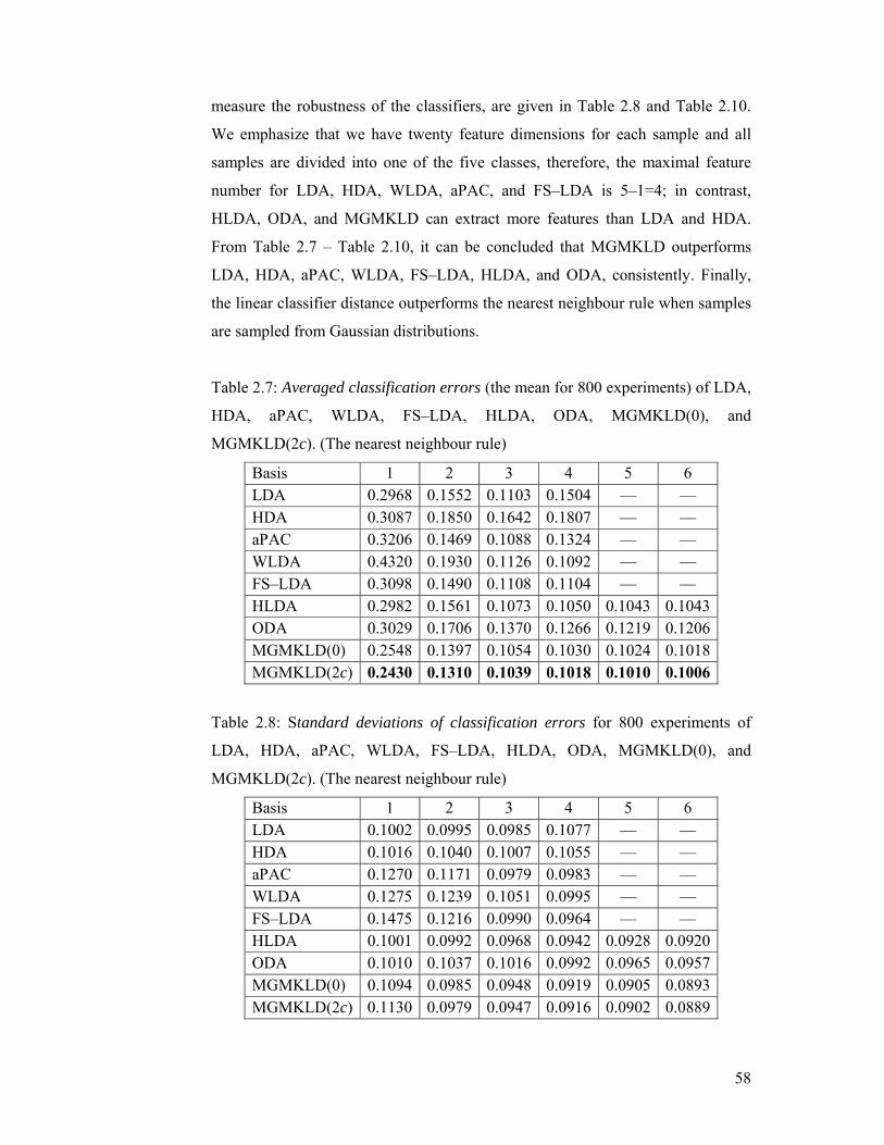
58
measure the robustness of the classifiers, are given in Table 2.8 and Table 2.10.
We emphasize that we have twenty feature dimensions for each sample and all
samples are divided into one of the five classes, therefore, the maximal feature
number for LDA, HDA, WLDA, aPAC, and FS–LDA is 5–1=4; in contrast,
HLDA, ODA, and MGMKLD can extract more features than LDA and HDA.
From Table 2.7 – Table 2.10, it can be concluded that MGMKLD outperforms
LDA, HDA, aPAC, WLDA, FS–LDA, HLDA, and ODA, consistently. Finally,
the linear classifier distance outperforms the nearest neighbour rule when samples
are sampled from Gaussian distributions.
Table 2.7: Averaged classification errors (the mean for 800 experiments) of LDA,
HDA, aPAC, WLDA, FS–LDA, HLDA, ODA, MGMKLD(0), and
MGMKLD(2c). (The nearest neighbour rule)
Basis 1 2 3 4 5 6 LDA 0.2968 0.1552 0.1103 0.1504 –– –– HDA 0.3087 0.1850 0.1642 0.1807 –– –– aPAC 0.3206 0.1469 0.1088 0.1324 –– –– WLDA 0.4320 0.1930 0.1126 0.1092 –– –– FS–LDA 0.3098 0.1490 0.1108 0.1104 –– –– HLDA 0.2982 0.1561 0.1073 0.1050 0.1043 0.1043 ODA 0.3029 0.1706 0.1370 0.1266 0.1219 0.1206 MGMKLD(0) 0.2548 0.1397 0.1054 0.1030 0.1024 0.1018 MGMKLD(2c) 0.2430 0.1310 0.1039 0.1018 0.1010 0.1006
Table 2.8: Standard deviations of classification errors for 800 experiments of
LDA, HDA, aPAC, WLDA, FS–LDA, HLDA, ODA, MGMKLD(0), and
MGMKLD(2c). (The nearest neighbour rule)
Basis 1 2 3 4 5 6 LDA 0.1002 0.0995 0.0985 0.1077 –– –– HDA 0.1016 0.1040 0.1007 0.1055 –– –– aPAC 0.1270 0.1171 0.0979 0.0983 –– –– WLDA 0.1275 0.1239 0.1051 0.0995 –– –– FS–LDA 0.1475 0.1216 0.0990 0.0964 –– –– HLDA 0.1001 0.0992 0.0968 0.0942 0.0928 0.0920 ODA 0.1010 0.1037 0.1016 0.0992 0.0965 0.0957 MGMKLD(0) 0.1094 0.0985 0.0948 0.0919 0.0905 0.0893 MGMKLD(2c) 0.1130 0.0979 0.0947 0.0916 0.0902 0.0889
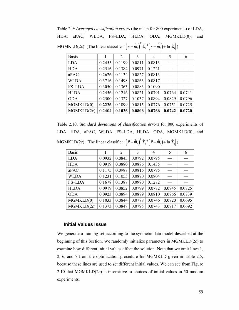
59
Table 2.9: Averaged classification errors (the mean for 800 experiments) of LDA,
HDA, aPAC, WLDA, FS–LDA, HLDA, ODA, MGMKLD(0), and
MGMKLD(2c). (The linear classifier ( ) ( )1ˆ ˆˆ ˆlnT
i i i ix m x m−− Σ − + Σr r r r )
Basis 1 2 3 4 5 6 LDA 0.2455 0.1199 0.0811 0.0813 –– –– HDA 0.2516 0.1384 0.0971 0.1221 –– –– aPAC 0.2626 0.1134 0.0827 0.0813 –– –– WLDA 0.3716 0.1498 0.0863 0.0817 –– –– FS–LDA 0.3050 0.1363 0.0883 0.1090 –– –– HLDA 0.2456 0.1216 0.0821 0.0791 0.0764 0.0741 ODA 0.2500 0.1327 0.1037 0.0894 0.0829 0.0796 MGMKLD(0) 0.2226 0.1099 0.0815 0.0776 0.0751 0.0725 MGMKLD(2c) 0.2404 0.1036 0.0806 0.0766 0.0742 0.0720
Table 2.10: Standard deviations of classification errors for 800 experiments of
LDA, HDA, aPAC, WLDA, FS–LDA, HLDA, ODA, MGMKLD(0), and
MGMKLD(2c). (The linear classifier ( ) ( )1ˆ ˆˆ ˆlnT
i i i ix m x m−− Σ − + Σr r r r )
Basis 1 2 3 4 5 6 LDA 0.0932 0.0843 0.0792 0.0795 –– –– HDA 0.0919 0.0880 0.0886 0.1435 –– –– aPAC 0.1175 0.0987 0.0816 0.0795 –– –– WLDA 0.1231 0.1055 0.0870 0.0804 –– –– FS–LDA 0.1678 0.1387 0.0980 0.1272 –– –– HLDA 0.0919 0.0852 0.0799 0.0772 0.0745 0.0725 ODA 0.0923 0.0894 0.0879 0.0810 0.0766 0.0739 MGMKLD(0) 0.1033 0.0844 0.0788 0.0746 0.0720 0.0695 MGMKLD(2c) 0.1373 0.0848 0.0795 0.0743 0.0717 0.0692
Initial Values Issue
We generate a training set according to the synthetic data model described at the
beginning of this Section. We randomly initialize parameters in MGMKLD(2c) to
examine how different initial values affect the solution. Note that we omit lines 1,
2, 6, and 7 from the optimization procedure for MGMKLD given in Table 2.5,
because these lines are used to set different initial values. We can see from Figure
2.10 that MGMKLD(2c) is insensitive to choices of initial values in 50 random
experiments.
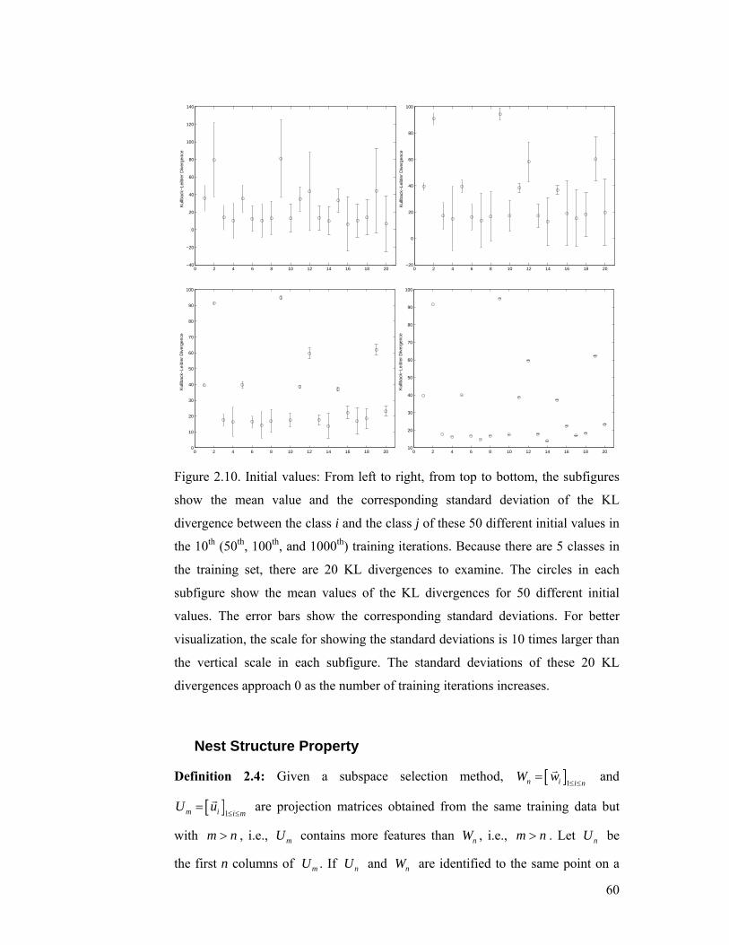
60
0 2 4 6 8 10 12 14 16 18 20−40
−20
0
20
40
60
80
100
120
140
Kul
lbac
k−Le
ible
r D
iver
genc
e
0 2 4 6 8 10 12 14 16 18 20−20
0
20
40
60
80
100
Kul
lbac
k−Le
ible
r D
iver
genc
e
0 2 4 6 8 10 12 14 16 18 200
10
20
30
40
50
60
70
80
90
100
Kul
lbac
k−Le
ible
r D
iver
genc
e
0 2 4 6 8 10 12 14 16 18 2010
20
30
40
50
60
70
80
90
100
Kul
lbac
k−Le
ible
r D
iver
genc
e
Figure 2.10. Initial values: From left to right, from top to bottom, the subfigures
show the mean value and the corresponding standard deviation of the KL
divergence between the class i and the class j of these 50 different initial values in
the 10th (50th, 100th, and 1000th) training iterations. Because there are 5 classes in
the training set, there are 20 KL divergences to examine. The circles in each
subfigure show the mean values of the KL divergences for 50 different initial
values. The error bars show the corresponding standard deviations. For better
visualization, the scale for showing the standard deviations is 10 times larger than
the vertical scale in each subfigure. The standard deviations of these 20 KL
divergences approach 0 as the number of training iterations increases.
Nest Structure Property
Definition 2.4: Given a subspace selection method, [ ]1n i i nW w
≤ ≤=
r and
[ ]1m i i mU u
≤ ≤=r are projection matrices obtained from the same training data but
with m n> , i.e., mU contains more features than nW , i.e., m n> . Let nU be
the first n columns of mU . If nU and nW are identified to the same point on a
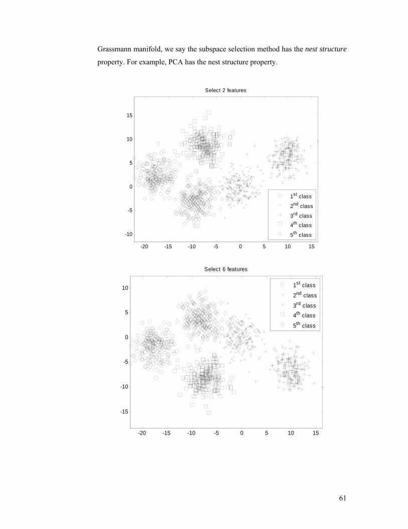
61
Grassmann manifold, we say the subspace selection method has the nest structure
property. For example, PCA has the nest structure property.
-20 -15 -10 -5 0 5 10 15
-10
-5
0
5
10
15
Select 2 features
1st class
2nd class
3rd class
4th class
5th class
-20 -15 -10 -5 0 5 10 15
-15
-10
-5
0
5
10
Select 6 features
1st class
2nd class
3rd class
4th class
5th class
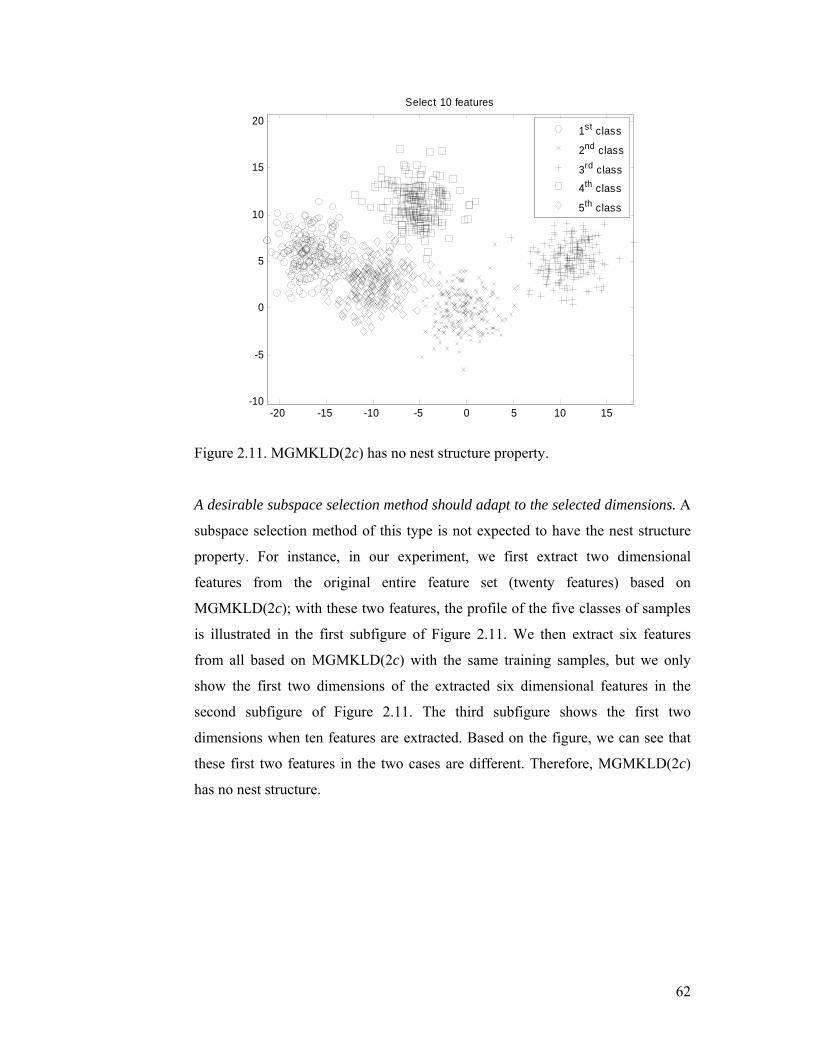
62
-20 -15 -10 -5 0 5 10 15-10
-5
0
5
10
15
20
Select 10 features
1st class
2nd class
3rd class
4th class
5th class
Figure 2.11. MGMKLD(2c) has no nest structure property.
A desirable subspace selection method should adapt to the selected dimensions. A
subspace selection method of this type is not expected to have the nest structure
property. For instance, in our experiment, we first extract two dimensional
features from the original entire feature set (twenty features) based on
MGMKLD(2c); with these two features, the profile of the five classes of samples
is illustrated in the first subfigure of Figure 2.11. We then extract six features
from all based on MGMKLD(2c) with the same training samples, but we only
show the first two dimensions of the extracted six dimensional features in the
second subfigure of Figure 2.11. The third subfigure shows the first two
dimensions when ten features are extracted. Based on the figure, we can see that
these first two features in the two cases are different. Therefore, MGMKLD(2c)
has no nest structure.
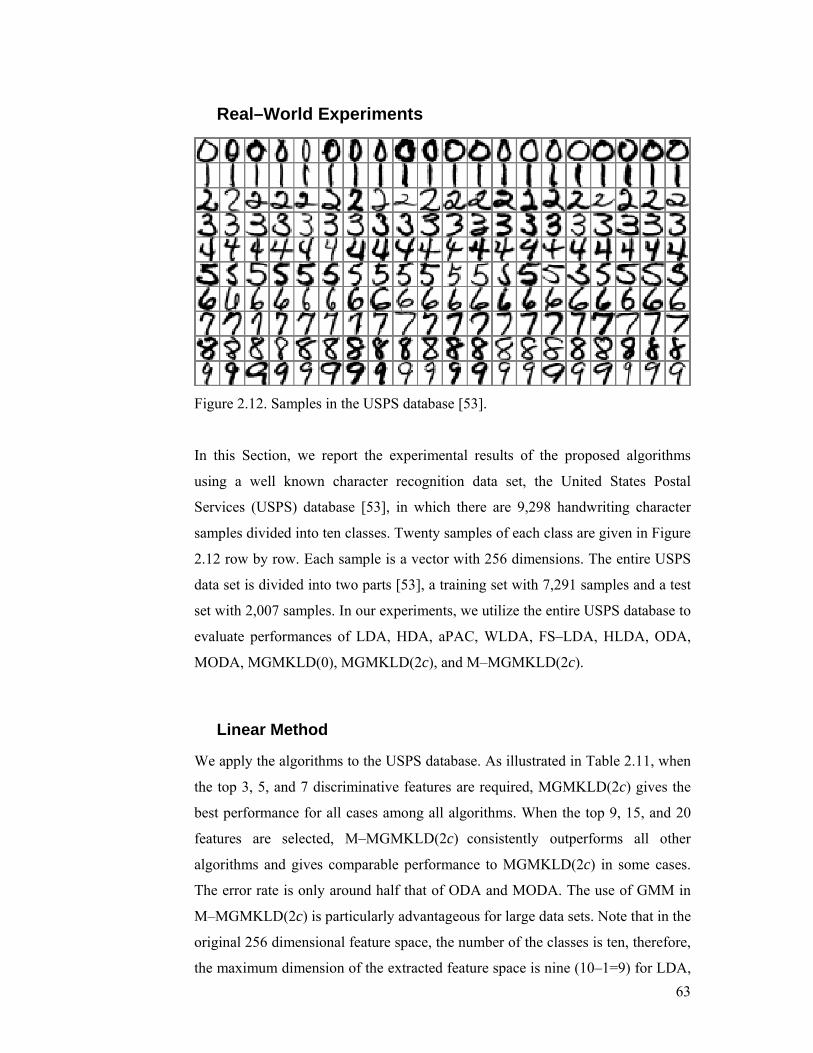
63
Real–World Experiments
Figure 2.12. Samples in the USPS database [53].
In this Section, we report the experimental results of the proposed algorithms
using a well known character recognition data set, the United States Postal
Services (USPS) database [53], in which there are 9,298 handwriting character
samples divided into ten classes. Twenty samples of each class are given in Figure
2.12 row by row. Each sample is a vector with 256 dimensions. The entire USPS
data set is divided into two parts [53], a training set with 7,291 samples and a test
set with 2,007 samples. In our experiments, we utilize the entire USPS database to
evaluate performances of LDA, HDA, aPAC, WLDA, FS–LDA, HLDA, ODA,
MODA, MGMKLD(0), MGMKLD(2c), and M–MGMKLD(2c).
Linear Method
We apply the algorithms to the USPS database. As illustrated in Table 2.11, when
the top 3, 5, and 7 discriminative features are required, MGMKLD(2c) gives the
best performance for all cases among all algorithms. When the top 9, 15, and 20
features are selected, M–MGMKLD(2c) consistently outperforms all other
algorithms and gives comparable performance to MGMKLD(2c) in some cases.
The error rate is only around half that of ODA and MODA. The use of GMM in
M–MGMKLD(2c) is particularly advantageous for large data sets. Note that in the
original 256 dimensional feature space, the number of the classes is ten, therefore,
the maximum dimension of the extracted feature space is nine (10–1=9) for LDA,
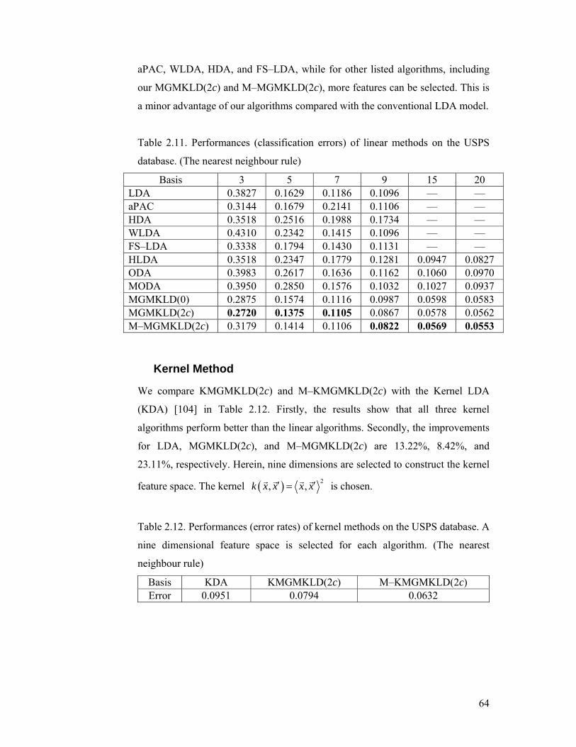
64
aPAC, WLDA, HDA, and FS–LDA, while for other listed algorithms, including
our MGMKLD(2c) and M–MGMKLD(2c), more features can be selected. This is
a minor advantage of our algorithms compared with the conventional LDA model.
Table 2.11. Performances (classification errors) of linear methods on the USPS
database. (The nearest neighbour rule)
Basis 3 5 7 9 15 20 LDA 0.3827 0.1629 0.1186 0.1096 –– –– aPAC 0.3144 0.1679 0.2141 0.1106 –– –– HDA 0.3518 0.2516 0.1988 0.1734 –– –– WLDA 0.4310 0.2342 0.1415 0.1096 –– –– FS–LDA 0.3338 0.1794 0.1430 0.1131 –– –– HLDA 0.3518 0.2347 0.1779 0.1281 0.0947 0.0827 ODA 0.3983 0.2617 0.1636 0.1162 0.1060 0.0970 MODA 0.3950 0.2850 0.1576 0.1032 0.1027 0.0937 MGMKLD(0) 0.2875 0.1574 0.1116 0.0987 0.0598 0.0583 MGMKLD(2c) 0.2720 0.1375 0.1105 0.0867 0.0578 0.0562 M–MGMKLD(2c) 0.3179 0.1414 0.1106 0.0822 0.0569 0.0553
Kernel Method
We compare KMGMKLD(2c) and M–KMGMKLD(2c) with the Kernel LDA
(KDA) [104] in Table 2.12. Firstly, the results show that all three kernel
algorithms perform better than the linear algorithms. Secondly, the improvements
for LDA, MGMKLD(2c), and M–MGMKLD(2c) are 13.22%, 8.42%, and
23.11%, respectively. Herein, nine dimensions are selected to construct the kernel
feature space. The kernel ( ) 2, ,k x x x x′ ′=r r r r is chosen.
Table 2.12. Performances (error rates) of kernel methods on the USPS database. A
nine dimensional feature space is selected for each algorithm. (The nearest
neighbour rule)
Basis KDA KMGMKLD(2c) M–KMGMKLD(2c) Error 0.0951 0.0794 0.0632

65
Summary
General averaged divergences analysis is proposed to enhance the conventional
Fisher–Rao linear discriminant analysis (LDA). LDA is one of the most important
subspace methods in pattern classification research and applications; however, it
has a tendency to merge together nearby classes when the features are projected to
a lower dimensional space. To reduce this merging, new criteria for subspace
selection are chosen. The new criteria are based on the geometric mean of the
divergences between different pairs of classes. Three new criteria are defined,
namely, 1) maximization of the geometric mean of the divergences; 2)
maximization of the geometric mean of normalized divergences; and 3)
maximization of the geometric mean of all divergences. The third criterion is a
combination of the first two criteria. Then, the multimodal extension and the
kernel extension of the maximization of the geometric mean of all divergences are
introduced as well. The divergence can be any Bregman divergence. In our
experiments we use the Kullback–Leibler divergence, which is a special case of
the Bregman divergence.
The new subspace selection methods are tested experimentally using synthetic
data and handwriting data from the USPS database [53]. The experiments show
that the third criterion, named the maximization of the geometric mean of all KL
divergences is more effective than LDA and its representatives. In the future, we
will utilize this method for other pattern classification tasks, for example
biometrics and bioinformatics.
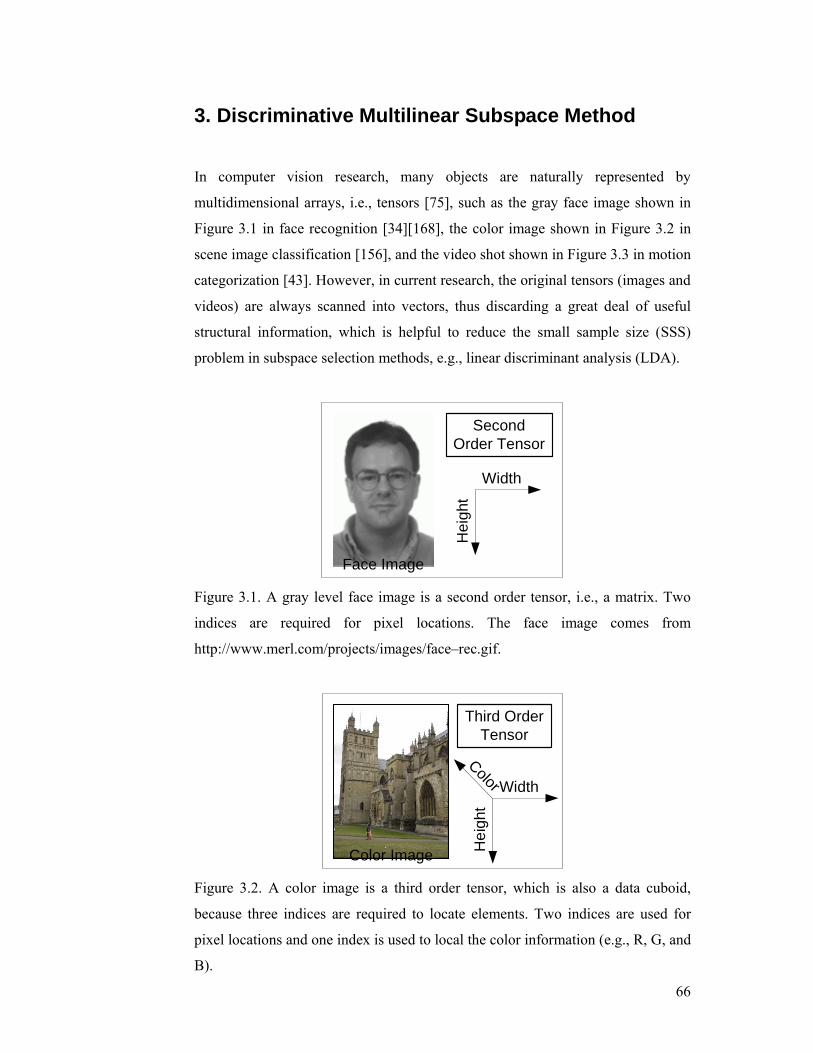
66
3. Discriminative Multilinear Subspace Method
In computer vision research, many objects are naturally represented by
multidimensional arrays, i.e., tensors [75], such as the gray face image shown in
Figure 3.1 in face recognition [34][168], the color image shown in Figure 3.2 in
scene image classification [156], and the video shot shown in Figure 3.3 in motion
categorization [43]. However, in current research, the original tensors (images and
videos) are always scanned into vectors, thus discarding a great deal of useful
structural information, which is helpful to reduce the small sample size (SSS)
problem in subspace selection methods, e.g., linear discriminant analysis (LDA).
Second Order Tensor
WidthH
eigh
t
Face Image Figure 3.1. A gray level face image is a second order tensor, i.e., a matrix. Two
indices are required for pixel locations. The face image comes from
http://www.merl.com/projects/images/face–rec.gif.
Third Order Tensor
Width
Hei
ght
Color
Color Image Figure 3.2. A color image is a third order tensor, which is also a data cuboid,
because three indices are required to locate elements. Two indices are used for
pixel locations and one index is used to local the color information (e.g., R, G, and
B).
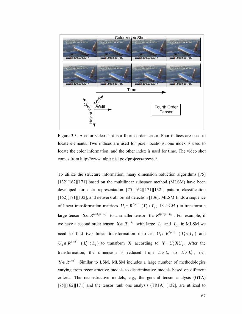
67
Fourth Order Tensor
Width
Hei
ght
Color Video Shot
Tim
eColor
Time
Figure 3.3. A color video shot is a fourth order tensor. Four indices are used to
locate elements. Two indices are used for pixel locations; one index is used to
locate the color information; and the other index is used for time. The video shot
comes from http://www–nlpir.nist.gov/projects/trecvid/.
To utilize the structure information, many dimension reduction algorithms [75]
[132][162][171] based on the multilinear subspace method (MLSM) have been
developed for data representation [75][162][171][132], pattern classification
[162][171][132], and network abnormal detection [136]. MLSM finds a sequence
of linear transformation matrices i iL LiU R ′×∈ ( i iL L′ < , 1 i M≤ ≤ ) to transform a
large tensor 1 2 ML L LR × ×∈X L to a smaller tensor 1 2 ML L LR ′ ′ ′× ×∈Y L . For example, if
we have a second order tensor 1 2L LR ×∈X with large 1L and 2L , in MLSM we
need to find two linear transformation matrices 1 11
L LU R ′×∈ ( 1 1L L′ < ) and
2 22
L LU R ′×∈ ( 2 2L L′ < ) to transform X according to 1 2TU U=Y X . After the
transformation, the dimension is reduced from 1 2L L× to 1 2L L′ ′× , i.e.,
1 2L LR ′ ′×∈Y . Similar to LSM, MLSM includes a large number of methodologies
varying from reconstructive models to discriminative models based on different
criteria. The reconstructive models, e.g., the general tensor analysis (GTA)
[75][162][171] and the tensor rank one analysis (TR1A) [132], are utilized to
68
generate low dimensional representations which preserve the original information
as much as possible. The discriminative models, e.g., the two dimensional linear
discriminant analysis (2DLDA) [173] and the general tensor discriminant analysis
(GTDA) [144][147], find low dimensional representations which preserve as
much as possible of the information required for reliable classification.
In this Chapter, we show that the SSS problem is reduced if the tensor structure of
data is retained. We also demonstrate that MLSM is a constrained version of the
linear subspace method (LSM), i.e., MLSM is equivalent to LSM combined with
constraints.
In this Chapter, we mainly focus on the discriminative MLSM, especially
2DLDA, which is a two dimensional extension of LDA. That is 2DLDA accepts
matrix type data as input while LDA accepts vector type data as input. The
effectiveness and the efficiency of 2DLDA for dimension reduction have been
demonstrated in face recognition. However, 2DLDA fails to converge during the
training stage. This nonconvergence has the following disadvantages: 1) it is
difficult to determine when to stop the training stage; and 2) different numbers of
training iterations lead to different recognition results. To solve the
nonconvergence problem in 2DLDA, we develop GTDA, which is an M
dimensional extension of LDA. That is GTDA accepts general tensors (e.g.,
vectors, matrices, data cuboids, and high dimensional arrays) as input. GTDA has
the following properties: 1) reduction of the SSS problem for subsequent
classification, e.g., by LDA; 2) preservation of the discriminative information in
training tensors; 3) provision with a converged iterative optimization algorithm,
which obtains a stable solution for GTDA; and 4) acceptance of general tensors as
input.
The organization of this Chapter is as follows. In §147, the mathematical
foundation, tensor algebra, of this thesis is briefly introduced. In §147, we
describe the relationship between the LSM algorithms and the MLSM algorithms.
In §147, the tensor rank one analysis based on the best rank one approximation is
reviewed. In §147, the general tensor analysis based on the best rank
( )1 2, , MR R RL approximation is reviewed. In §147, we analyze the
nonconvergence issue of the 2DLDA for discriminative subspace selection. In
§147, we develop GTDA and GTDA’s manifold learning extension is given in
§147. To examine the effectiveness of GTDA, it is applied for human gait

69
recognition and the performance evaluation is given in §147. Finally, the
summary of this Chapter is given in §147 and the relevant deductions and proofs
in this Chapter are given in §147.
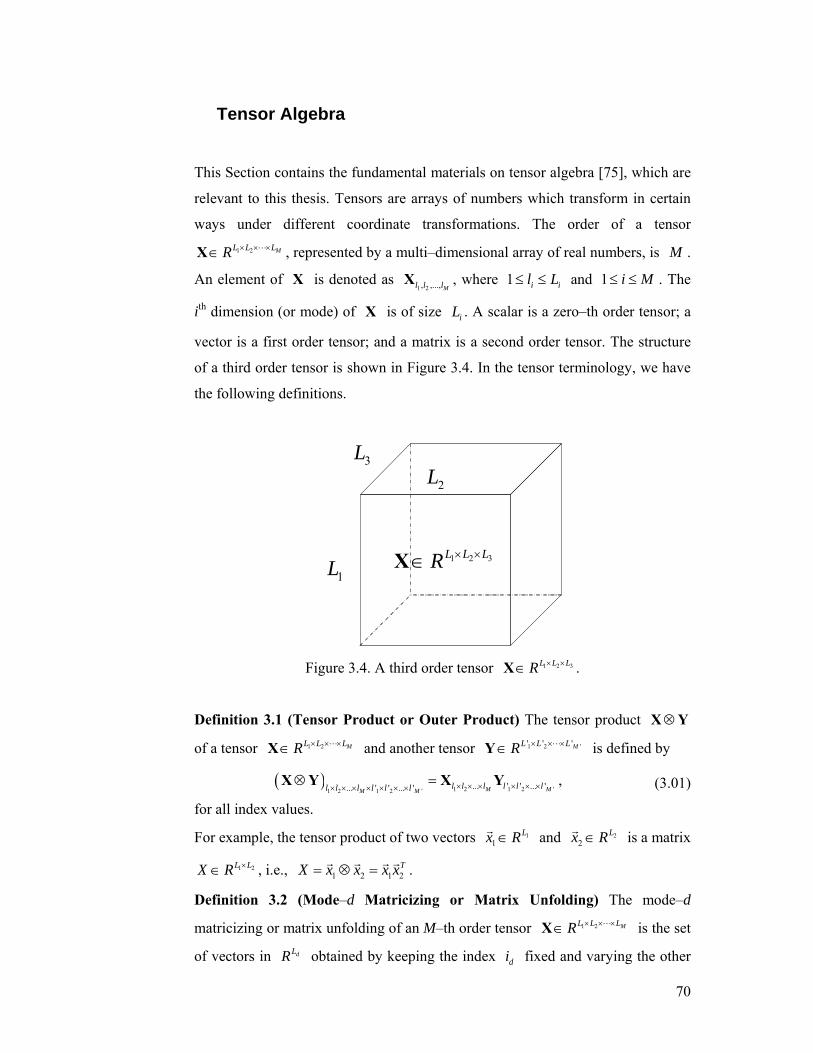
70
Tensor Algebra
This Section contains the fundamental materials on tensor algebra [75], which are
relevant to this thesis. Tensors are arrays of numbers which transform in certain
ways under different coordinate transformations. The order of a tensor 1 2 ML L LR × × ×∈X L , represented by a multi–dimensional array of real numbers, is M .
An element of X is denoted as 1 2, ,..., Ml l lX , where 1 i il L≤ ≤ and 1 i M≤ ≤ . The
ith dimension (or mode) of X is of size iL . A scalar is a zero–th order tensor; a
vector is a first order tensor; and a matrix is a second order tensor. The structure
of a third order tensor is shown in Figure 3.4. In the tensor terminology, we have
the following definitions.
1 2 3L L LR × ×∈X1L
2L3L
Figure 3.4. A third order tensor 1 2 3L L LR × ×∈X .
Definition 3.1 (Tensor Product or Outer Product) The tensor product ⊗X Y
of a tensor 1 2 ML L LR × × ×∈X L and another tensor 1 2 '' ' 'ML L LR × × ×∈Y L is defined by
( )1 2 1 2 '1 2 1 2 '
... ' ' ... '... ' ' ... ' M MM Ml l l l l ll l l l l l × × × × × ×× × × × × × ×
⊗ =X Y X Y , (3.01)
for all index values.
For example, the tensor product of two vectors 11
Lx R∈r and 2
2Lx R∈
r is a matrix
1 2L LX R ×∈ , i.e., 1 2 1 2TX x x x x= ⊗ =
r r r r .
Definition 3.2 (Mode–d Matricizing or Matrix Unfolding) The mode–d
matricizing or matrix unfolding of an M–th order tensor 1 2 ML L LR × × ×∈X L is the set
of vectors in dLR obtained by keeping the index di fixed and varying the other
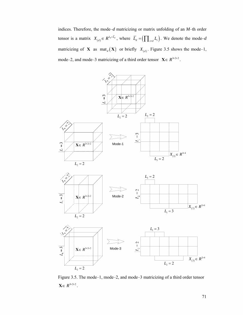
71
indices. Therefore, the mode–d matricizing or matrix unfolding of an M–th order
tensor is a matrix ( )d dL L
dX R ×∈ , where ( )d ii dL L
≠= ∏ . We denote the mode–d
matricizing of X as ( )matd X or briefly ( )dX . Figure 3.5 shows the mode–1,
mode–2, and mode–3 matricizing of a third order tensor 3 2 2R × ×∈X .
2 2L =
3 2 2R × ×∈X
2 2L =
3 2 2R × ×∈X
2 2L =
3 2 2R × ×∈X
Mode-1
Mode-2
Mode-3
2 2L =
3 2 2R × ×∈X
2 2L =
3 2L =
1 3L =
3 2L =
2 2L =
1 3L =
( )3 4
1X R ×∈
( )2 6
2X R ×∈
( )2 6
3X R ×∈
Figure 3.5. The mode–1, mode–2, and mode–3 matricizing of a third order tensor
3 2 2R × ×∈X .
72
Definition 3.3 (Tensor Contraction) The contraction of a tensor is obtained by
equating two indices and summing over all values of repeated indices. Contraction
reduces the tensor order by 2.
A suitable notation for contraction is the Einstein’s summation convention10. For
example, the tensor product of two vectors , Nx y R∈r r is Z x y= ⊗
r r ; and the
contraction of Z is TiiZ x y x y= ⋅ =
r r r r , where the repeated indices imply
summation. The value of iiZ is the inner product of xr and yr . In general, for
tensors 1 1M ML L L LR ′′ ′× × × × ×∈X L L and 1 1M ML L L LR ′′′′ ′′× × × × ×∈Y L L , the contraction on the
tensor product ⊗X Y is
( )( ) ( ) ( )1
1 1 1 11 1 1
; 1: 1:M
M M M MM
L L
l l l l l l l ll l
M M′ ′′′ ′ ′′ ′′× × × × × × × × × ×
= =
⊗ =∑ ∑X Y X YL L L L
L , (3.02)
In this thesis, when the convention is conducted on all indices except the ith index
on the tensor product of X and Y in 1 2 ML L LR × × ×L , we denote this procedure as
( )( ) ( )( )
( ) ( )
( ) ( ) ( ) ( )
1 11
1 1 1 1 1 11 1 11 1 1 1
; ; 1: 1, 1: 1: 1, 1:
mat mat ,
i i M
i i i M i i i Mi i M
L LL L
l l l l l l l l l ll l l l
T Ti i i i
i i i i M i i M
X Y
− +
− + − +− +
× × × × × × × × × × × ×= = = =
⊗ = ⊗ − + − +
=
= =
∑ ∑ ∑ ∑
X Y X Y
X Y
X Y
L L L LL L (3.03)
and ( )( ); i iL Li i R ×⊗ ∈X Y .
Definition 3.4 (Mode–d product) The mode–d product d U×X of a tensor
1 2 ... ML L LR × × ×∈X and a matrix 'd dL LU R ×∈ is an 1 2 1 1'd d dL L L L L− +× × × × × ×L
ML×L tensor defined by
( ) ( )( )( )
1 2 1 11 2 1 1
; 2 ,
d d d M d dd d d Md
d l l l l l l l ll l l l l ll
U U
U d
− +− +′× × × × × × × ×′× × × × × × ×
′
× =
= ⊗
∑X X
X
L LL L
(3.04)
for all index values. The mode–d product is a type of contraction.
Based on the definition of Mode–d product, we have
( ) ( )d t t dU V V U× × = × ×X X (3.05)
10 “When any two subscripts in a tensor expression are given the same symbol, it is implied that the convention is formed.” –––––A. Einstein, Die Grundlage der Allgemeinen Relativitatstheorie, Ann. Phys., 49:769, 1916.
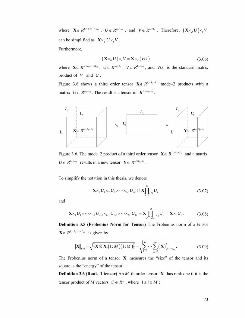
73
where 1 2 ML L LR × × ×∈X L , d dL LU R ′ ×∈ , and t tL LV R ′×∈ . Therefore, ( )d tU V× ×X
can be simplified as d tU V× ×X .
Furthermore,
( ) ( )d t dU V VU× × = ×X X (3.06)
where 1 2 ML L LR × × ×∈X L , d dL LU R ′ ×∈ , d dL LV R ′′ ′×∈ , and VU is the standard matrix
product of V and U .
Figure 3.6 shows a third order tensor 1 2 3L L LR × ×∈X mode–2 products with a
matrix 2 2L LU R ′ ×∈ . The result is a tensor in 1 2 3L L LR ′× × .
1 2 3L L LR × ×∈X1L
2L3L
2×
2L
2L′ =1 2 3L L LR ′× ×∈Y
1L
2L′3L
Figure 3.6. The mode–2 product of a third order tensor 1 2 3L L LR × ×∈X and a matrix 2 2L LU R ′ ×∈ results in a new tensor 1 2 3L L LR ′× ×∈Y .
To simplify the notation in this thesis, we denote
1 1 2 21
k
M
M M kk
U U U U×=
× × × × ∏X XL (3.07)
and
1 1 1 1 1 11;
d
M
i i i i M M d i id d i
U U U U U U− − + + ×= ≠
× × × × × × = ×∏X X XL L . (3.08)
Definition 3.5 (Frobenius Norm for Tensor) The Frobenius norm of a tensor 1 2 ML L LR × × ×∈X L is given by
( )( ) ( )1
11
2
1 1
; 1: 1: .M
MM
L L
l lFrol l
M M× ×
= =
= ⊗ = ∑ ∑X X X XL
L (3.09)
The Frobenius norm of a tensor X measures the “size” of the tensor and its
square is the “energy” of the tensor.
Definition 3.6 (Rank–1 tensor) An M–th order tensor X has rank one if it is the
tensor product of M vectors iLiu R∈r , where 1 i M≤ ≤ :
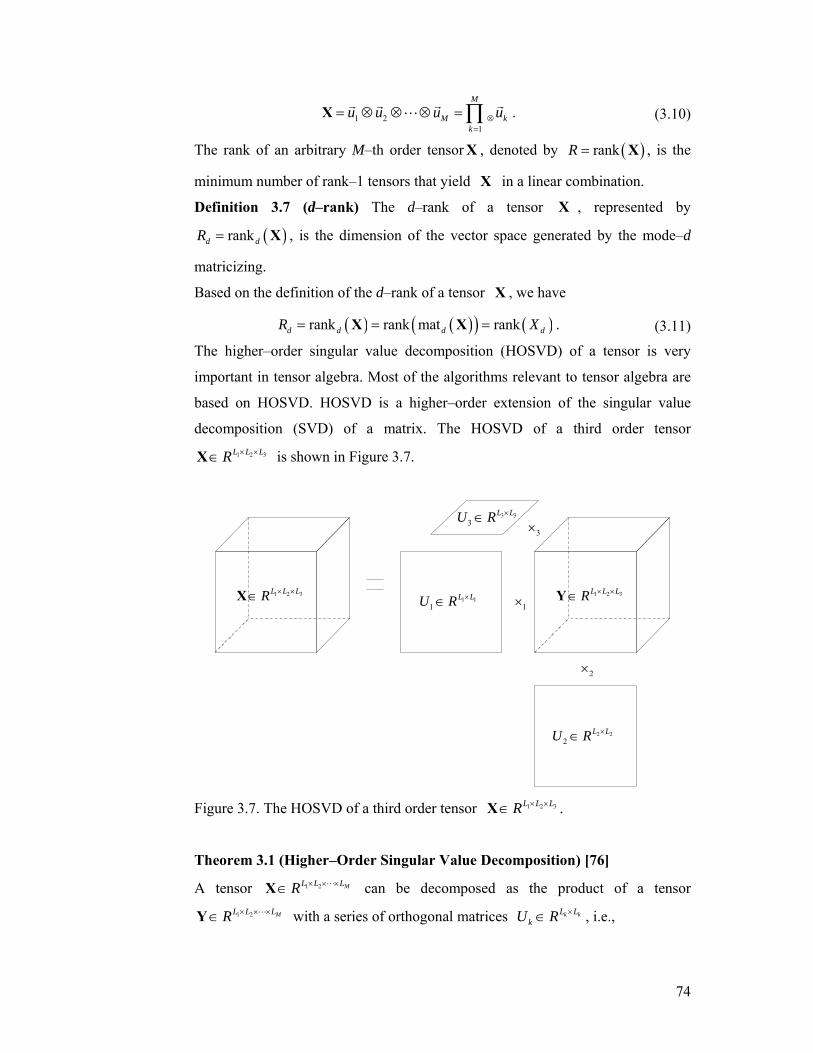
74
1 21
M
M kk
u u u u⊗=
= ⊗ ⊗ ⊗ =∏X r r r rL . (3.10)
The rank of an arbitrary M–th order tensor X , denoted by ( )rankR = X , is the
minimum number of rank–1 tensors that yield X in a linear combination.
Definition 3.7 (d–rank) The d–rank of a tensor X , represented by
( )rankd dR = X , is the dimension of the vector space generated by the mode–d
matricizing.
Based on the definition of the d–rank of a tensor X , we have
( ) ( )( ) ( )rank rank mat rankd d d dR X= = =X X . (3.11)
The higher–order singular value decomposition (HOSVD) of a tensor is very
important in tensor algebra. Most of the algorithms relevant to tensor algebra are
based on HOSVD. HOSVD is a higher–order extension of the singular value
decomposition (SVD) of a matrix. The HOSVD of a third order tensor 1 2 3L L LR × ×∈X is shown in Figure 3.7.
1 2 3L L LR × ×∈X 1 2 3L L LR × ×∈Y1 11
L LU R ×∈
2 22
L LU R ×∈
1×
2×
3 33
L LU R ×∈3×
Figure 3.7. The HOSVD of a third order tensor 1 2 3L L LR × ×∈X .
Theorem 3.1 (Higher–Order Singular Value Decomposition) [76]
A tensor 1 2 ML L LR × × ×∈X L can be decomposed as the product of a tensor 1 2 ML L LR × × ×∈Y L with a series of orthogonal matrices k kL L
kU R ×∈ , i.e.,
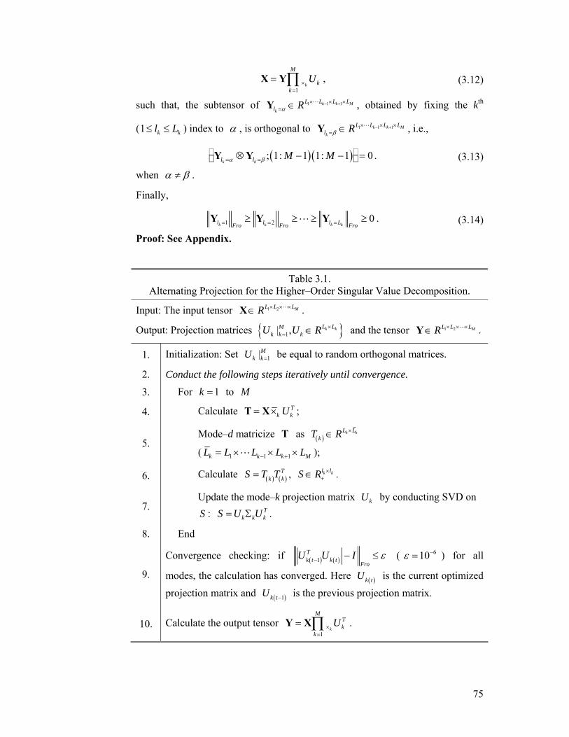
75
1k
M
kk
U×=
= ∏X Y , (3.12)
such that, the subtensor of 1 1 1k k M
k
L L L Ll Rα
− +× × ×= ∈Y L , obtained by fixing the kth
(1 k kl L≤ ≤ ) index to α , is orthogonal to 1 1 1k k M
k
L L L Ll Rβ
− +× × ×= ∈Y L , i.e.,
( )( ); 1: 1 1: 1 0k kl l M Mα β= =⊗ − − =Y Y . (3.13)
when α β≠ .
Finally,
1 2 0k k k kl l l LFro Fro Fro= = =≥ ≥ ≥ ≥Y Y YL . (3.14)
Proof: See Appendix.
Table 3.1. Alternating Projection for the Higher–Order Singular Value Decomposition.
Input: The input tensor 1 2 ML L LR × × ×∈X L .
Output: Projection matrices { }1| , k kL LMk k kU U R ×
= ∈ and the tensor 1 2 ML L LR × × ×∈Y L .
1. Initialization: Set 1|Mk kU = be equal to random orthogonal matrices.
2. Conduct the following steps iteratively until convergence.
3. For 1k = to M
4. Calculate Tk kU= ×T X ;
5. Mode–d matricize T as ( )
k kL LkT R ×∈
( 1 1 1k k k ML L L L L− += × × ×L );
6. Calculate ( ) ( )T
k kS T T= , k kl lS R ×+∈ .
7. Update the mode–k projection matrix kU by conducting SVD on S : T
k k kS U U= Σ .
8. End
9.
Convergence checking: if ( ) ( )1Tk t k t
FroU U I ε− − ≤ ( 610ε −= ) for all
modes, the calculation has converged. Here ( )k tU is the current optimized
projection matrix and ( )1k tU − is the previous projection matrix.
10. Calculate the output tensor 1
k
MTk
k
U×=
= ∏Y X .

76
There is no closed form solution for HOSVD. In this thesis, an alternating
projection method is used to obtain a solution for HOSVD, as shown in Table 3.1.
77
The Relationship between LSM and MLSM
Suppose: 1) we have a dimension reduction algorithm 1A , which finds a sequence
of linear transformation matrices i iL LiU R ′×∈ ( i iL L′ < , 1 i M≤ ≤ ) to transform a
large tensor 1 2 ML L LR × ×∈X L to a smaller tensor 1 21
ML L LR ′ ′ ′× ×∈Y L , i.e.,
1 1 1 2 2T T T
M MU U U= × × × ×Y X L ; and 2) we have another dimension reduction
algorithm 2A , which finds a linear transformation matrix L LU R ′×∈
( 1 2 ML L L L= × ×L and 1 2 ML L L L′ ′ ′ ′= × ×L ; i iL L′ < ) to transform a high
dimensional vector ( )vectx = Xr to a lower dimensional vector ( )2 2vecty = Yr ,
i.e., 2Ty U x=
r r , where ( )vect ⋅ is the vectorization operator; Lx R∈r and
2Ly R ′∈
r . According to [181], we know
( )( )
( ) ( )
1 1
1 1 2 2
1 2
vect
vect
vect .
T T TM M
TM
y
U U U
U U U
=
= × × × ×
= ⊗ ⊗ ⊗
Y
X
X
r
L
L
(3.15)
Therefore, if 1 2 MU U U U= ⊗ ⊗ ⊗L , 2 1y y=r r . That is the algorithm 1A is equal
to the algorithm 2A , if the linear transformation matrix L LU R ′×∈ in 2A is
equal to 1 2 MU U U U= ⊗ ⊗ ⊗L 11.
The tensor representation helps to reduce the number of parameters needed to
model data. In 1A , there are 1 1
Mi ii
N L L=
′= ∑ parameters. While in 2A , there are
2 1 1
M Mi ii i
N L L= =
′=∏ ∏ parameters. In statistical learning, we usually require that
the number of the training samples is larger than the number of parameters to
model these training samples for linear algorithms. In the training stage of the
MLSM based learning algorithms, we usually use the alternating projection
method to obtain a solution, i.e., the linear projection matrices are obtained
independently, so we only need about { }0 max i iiN L L′= training samples to
obtain a solution. However, 2N training samples are required to obtain a
11 In (3.15), we conduct the reshape operation on 1 2 MU U U= ⊗ ⊗ ⊗U L . That is, originally U lies in 1 1 2 2 M ML L L L L LR ′ ′ ′× × × × × ×L and after the reshape operation U is transformed to V in
( ) ( )1 2 1 2M ML L L L L LR ′ ′ ′× × × × × × ×L L . Then, we can apply the transpose operation on V .
78
solution for LSM based learning algorithms. That is the MLSM based learning
algorithms require a much smaller number of training samples than LSM based
learning algorithms, because 0 2N N . Therefore, the tensor representation helps
to reduce the small sample size (SSS) problem described in Chapter 2.
There is a long history of methods to reduce the number of parameters needed to
model the data by introducing constraints. Take the methods in Gaussian
distribution estimation as an example12: when the data consist of only a few
training samples embedded in a high dimensional space, we always add some
constraints to the covariance matrix, for example by requiring the covariance
matrix to be a diagonal matrix. Therefore, to better characterize or classify natural
data, a scheme should preserve as many as possible of the original constraints.
When the training samples are limited, these constraints help to give reasonable
solutions to classification problems.
Based on the discussions above, we have the following results:
1) when the number of the training samples is limited, the vectorization operation
always leads to the SSS problem. That is, for a small size training set, we need to
use the MLSM based learning algorithms, because the LSM based learning
algorithms will over–fit the data. The vectorization of a tensor into a vector
makes it harder to keep track of the information in spatial constraints. For
example, two 4–neighbor connected pixels in an image may be widely separated
from each other after a vectorization;
2) when the number of training samples is large, the MLSM based learning
algorithms will under–fit the data. In this case, the vectorization operation for the
data is helpful because it increases the number of parameters available to model
the data.
12 Constraints in MLSM are justified by the form of the data. However, constrains in the example are ad hoc.
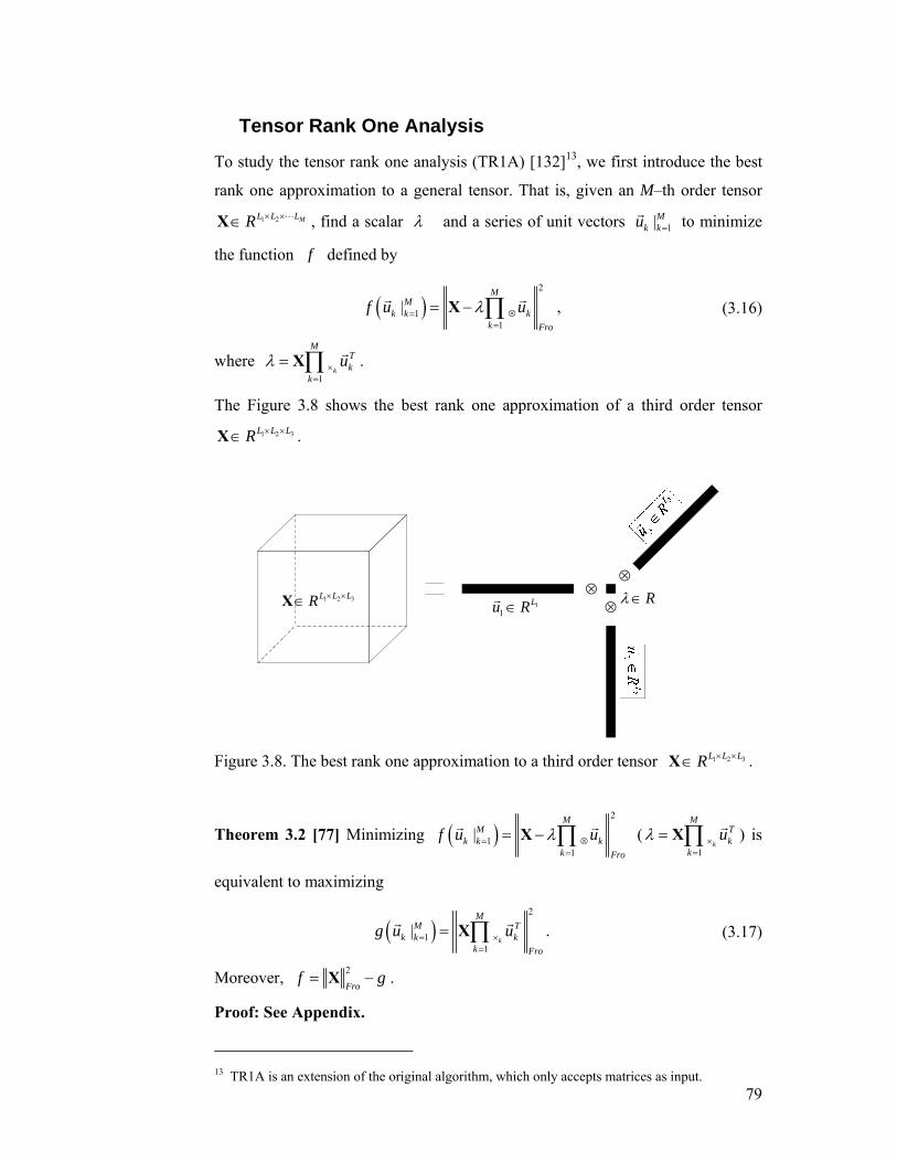
79
Tensor Rank One Analysis
To study the tensor rank one analysis (TR1A) [132]13, we first introduce the best
rank one approximation to a general tensor. That is, given an M–th order tensor 1 2 ML L LR × ×∈X L , find a scalar λ and a series of unit vectors 1|Mk ku =
r to minimize
the function f defined by
( )2
11
|M
Mk k k
k Fro
f u uλ= ⊗=
= − ∏Xr r , (3.16)
where 1
k
MTk
k
uλ ×=
= ∏X r .
The Figure 3.8 shows the best rank one approximation of a third order tensor 1 2 3L L LR × ×∈X .
1 2 3L L LR × ×∈X 11
Lu R∈r
⊗⊗
⊗Rλ∈
Figure 3.8. The best rank one approximation to a third order tensor 1 2 3L L LR × ×∈X .
Theorem 3.2 [77] Minimizing ( )2
11
|M
Mk k k
k Fro
f u uλ= ⊗=
= − ∏Xr r (1
k
MTk
k
uλ ×=
= ∏X r ) is
equivalent to maximizing
( )2
11
|k
MM T
k k kk Fro
g u u= ×=
= ∏Xr r . (3.17)
Moreover, 2
Frof g= −X .
Proof: See Appendix.
13 TR1A is an extension of the original algorithm, which only accepts matrices as input.
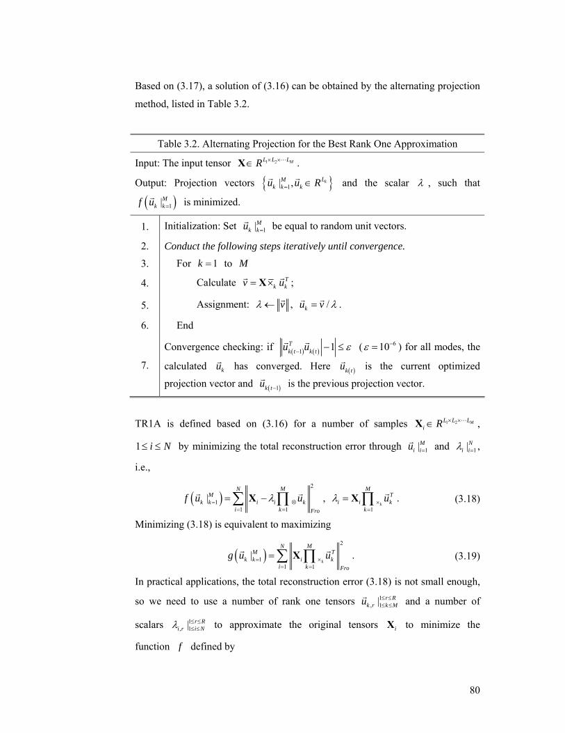
80
Based on (3.17), a solution of (3.16) can be obtained by the alternating projection
method, listed in Table 3.2.
Table 3.2. Alternating Projection for the Best Rank One Approximation
Input: The input tensor 1 2 ML L LR × ×∈X L .
Output: Projection vectors { }1| , kLMk k ku u R= ∈r r and the scalar λ , such that
( )1|Mk kf u =r is minimized.
1. Initialization: Set 1|Mk ku =r be equal to random unit vectors.
2. Conduct the following steps iteratively until convergence.
3. For 1k = to M
4. Calculate Tk kv u= ×Xr r ;
5. Assignment: vλ ←r , /ku v λ=
r r .
6. End
7.
Convergence checking: if ( ) ( )1 1Tk t k tu u ε− − ≤r r ( 610ε −= ) for all modes, the
calculated kur has converged. Here ( )k tur is the current optimized
projection vector and ( )1k tu −
r is the previous projection vector.
TR1A is defined based on (3.16) for a number of samples 1 2 ML L Li R × ×∈X L ,
1 i N≤ ≤ by minimizing the total reconstruction error through 1|Mi iu =r and 1|Ni iλ = ,
i.e.,
( )2
11 1
|MN
Mk k i i k
i k Fro
f u uλ= ⊗= =
= −∑ ∏Xr r , 1
k
MT
i i kk
uλ ×=
= ∏X r . (3.18)
Minimizing (3.18) is equivalent to maximizing
( )2
11 1
|k
MNM T
k k i ki k Fro
g u u= ×= =
=∑ ∏Xr r . (3.19)
In practical applications, the total reconstruction error (3.18) is not small enough,
so we need to use a number of rank one tensors 1, 1|
r Rk r k Mu ≤ ≤
≤ ≤r and a number of
scalars 1, 1|
r Ri r i Nλ ≤ ≤
≤ ≤ to approximate the original tensors iX to minimize the
function f defined by
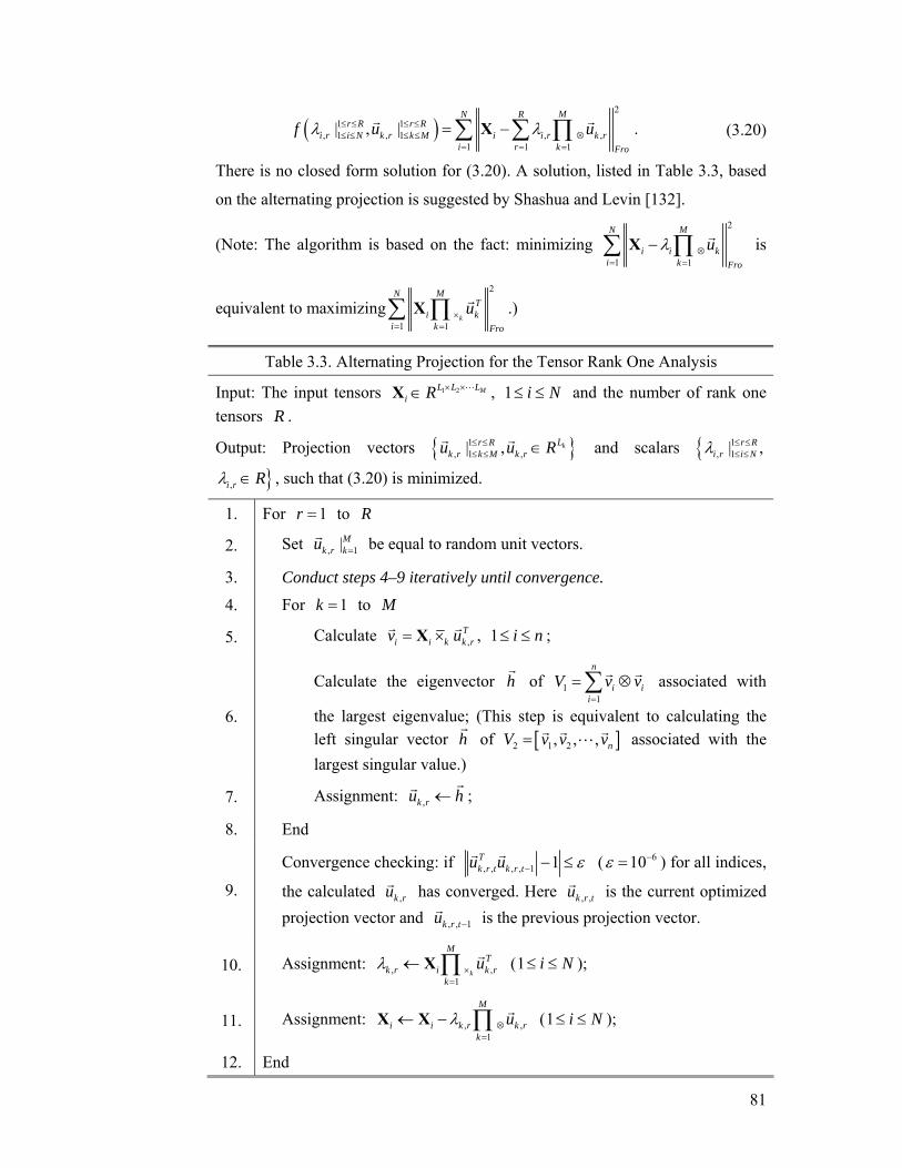
81
( )2
1 1, 1 , 1 , ,
1 1 1
| , |MN R
r R r Ri r i N k r k M i i r k r
i r k Fro
f u uλ λ≤ ≤ ≤ ≤≤ ≤ ≤ ≤ ⊗
= = =
= −∑ ∑ ∏Xr r . (3.20)
There is no closed form solution for (3.20). A solution, listed in Table 3.3, based
on the alternating projection is suggested by Shashua and Levin [132].
(Note: The algorithm is based on the fact: minimizing 2
1 1
MN
i i ki k Fro
uλ ⊗= =
−∑ ∏X r is
equivalent to maximizing2
1 1k
MNT
i ki k Fro
u×= =∑ ∏X r .)
Table 3.3. Alternating Projection for the Tensor Rank One Analysis
Input: The input tensors 1 2 ML L Li R × ×∈X L , 1 i N≤ ≤ and the number of rank one
tensors R .
Output: Projection vectors { }1, 1 ,| , kLr R
k r k M k ru u R≤ ≤≤ ≤ ∈
r r and scalars { 1, 1| ,r R
i r i Nλ ≤ ≤≤ ≤
},i r Rλ ∈ , such that (3.20) is minimized.
1. For 1r = to R
2. Set , 1|Mk r ku =r be equal to random unit vectors.
3. Conduct steps 4–9 iteratively until convergence.
4. For 1k = to M
5. Calculate ,T
i i k k rv u= ×Xr r , 1 i n≤ ≤ ;
6.
Calculate the eigenvector hr
of 11
n
i ii
V v v=
= ⊗∑ r r associated with
the largest eigenvalue; (This step is equivalent to calculating the left singular vector h
r of [ ]2 1 2, , , nV v v v=
r r rL associated with the
largest singular value.)
7. Assignment: ,k ru h←rr ;
8. End
9.
Convergence checking: if , , , , 1 1Tk r t k r tu u ε− − ≤r r ( 610ε −= ) for all indices,
the calculated ,k rur has converged. Here , ,k r tur is the current optimized projection vector and , , 1k r tu −
r is the previous projection vector.
10. Assignment: , ,1
k
MT
k r i k rk
uλ ×=
← ∏X r (1 i N≤ ≤ );
11. Assignment: , ,1
M
i i k r k rk
uλ ⊗=
← − ∏X X r (1 i N≤ ≤ );
12. End
82
Based on the procedure to obtain a solution for TR1A listed in Table 3.3, we can
calculate the scalars 1|Rr rλ = for any given tensor X through the following
iterative procedure: 1). Calculate ,1
k
MT
r k rk
uλ ×=
= ∏X r ; 2) Assign
,1
M
r k rk
uλ ⊗=
← − ∏X X r , 1 r R≤ ≤ . Based on TR1A, a general tensor is represented
by a sequence of rank one approximations.
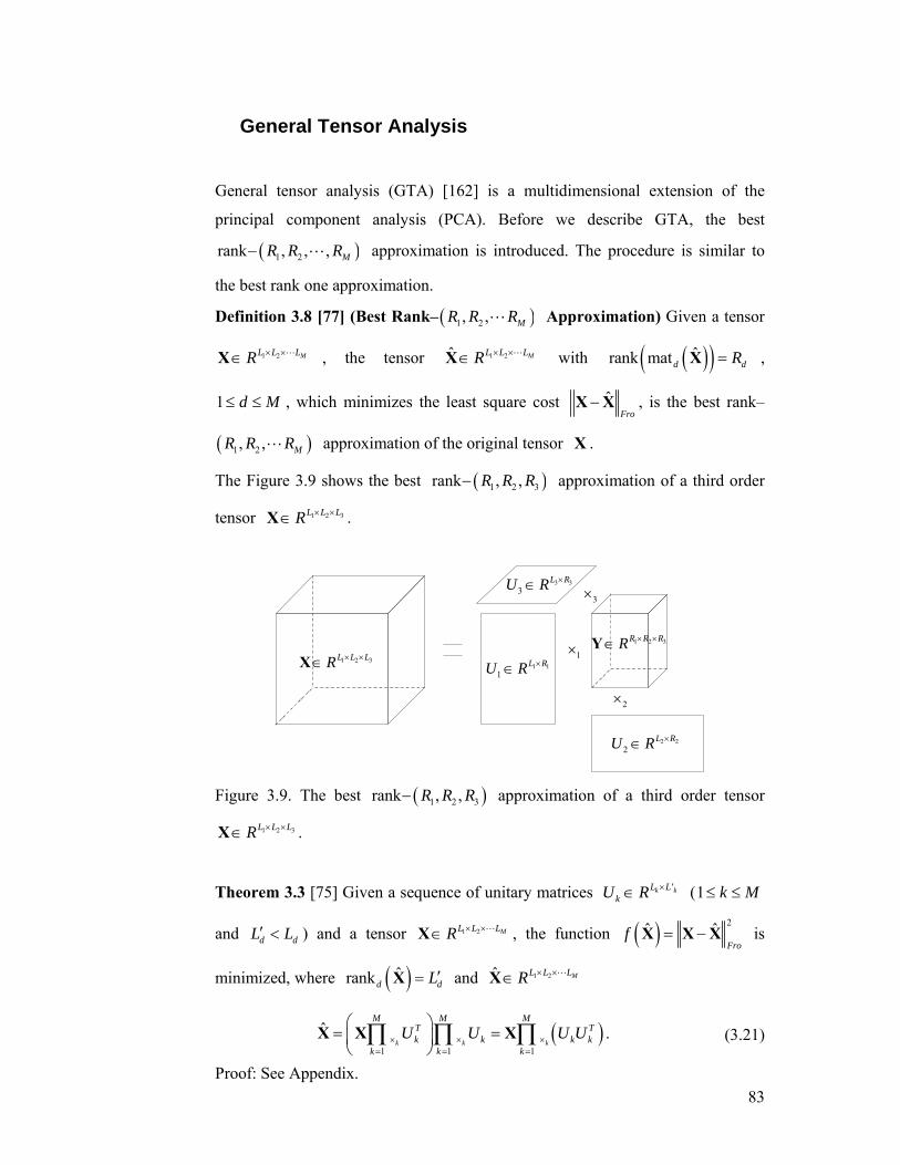
83
General Tensor Analysis
General tensor analysis (GTA) [162] is a multidimensional extension of the
principal component analysis (PCA). Before we describe GTA, the best
( )1 2rank , , , MR R R− L approximation is introduced. The procedure is similar to
the best rank one approximation.
Definition 3.8 [77] (Best Rank– ( )1 2, , MR R RL Approximation) Given a tensor
1 2 ML L LR × ×∈X L , the tensor 1 2ˆ ML L LR × ×∈X L with ( )( )ˆrank matd dR=X ,
1 d M≤ ≤ , which minimizes the least square cost ˆFro
−X X , is the best rank–
( )1 2, , MR R RL approximation of the original tensor X .
The Figure 3.9 shows the best ( )1 2 3rank , ,R R R− approximation of a third order
tensor 1 2 3L L LR × ×∈X .
1 2 3L L LR × ×∈X1 2 3R R RR × ×∈Y
1 11
L RU R ×∈
2 22
L RU R ×∈
1×
2×
3 33
L RU R ×∈3×
Figure 3.9. The best ( )1 2 3rank , ,R R R− approximation of a third order tensor
1 2 3L L LR × ×∈X .
Theorem 3.3 [75] Given a sequence of unitary matrices 'k kL LkU R ×∈ (1 k M≤ ≤
and d dL L′ < ) and a tensor 1 2 ML L LR × ×∈X L , the function ( ) 2ˆ ˆFro
f = −X X X is
minimized, where ( )ˆrankd dL′=X and 1 2ˆ ML L LR × ×∈X L
( )1 1 1
ˆk k k
M M MT Tk k k k
k k k
U U U U× × ×= = =
⎛ ⎞= =⎜ ⎟⎝ ⎠∏ ∏ ∏X X X . (3.21)
Proof: See Appendix.
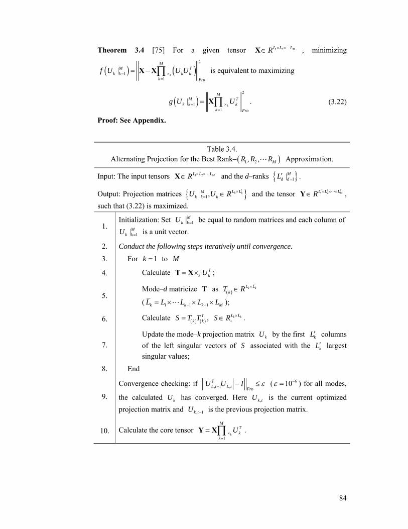
84
Theorem 3.4 [75] For a given tensor 1 2 ML L LR × ×∈X L , minimizing
( ) ( )2
11
|k
MM T
k k k kk Fro
f U U U= ×=
= − ∏X X is equivalent to maximizing
( )2
11
|k
MM T
k k kk Fro
g U U= ×=
= ∏X . (3.22)
Proof: See Appendix.
Table 3.4. Alternating Projection for the Best Rank– ( )1 2, , MR R RL Approximation.
Input: The input tensors 1 2 ML L LR × ×∈X L and the d–ranks { }1|Md dL =′ .
Output: Projection matrices { }1| , k kL LMk k kU U R ′×
= ∈ and the tensor 1 2 ML L LR ′ ′ ′× × ×∈Y L , such that (3.22) is maximized.
1. Initialization: Set 1|Mk kU = be equal to random matrices and each column of
1|Mk kU = is a unit vector.
2. Conduct the following steps iteratively until convergence.
3. For 1k = to M
4. Calculate Tk kU= ×T X ;
5. Mode–d matricize T as ( )
k kL LkT R ×∈
( 1 1 1k k k ML L L L L− += × × ×L );
6. Calculate ( ) ( )T
k kS T T= , k kL LS R ×+∈ .
7. Update the mode–k projection matrix kU by the first kL′ columns of the left singular vectors of S associated with the kL′ largest singular values;
8. End
9.
Convergence checking: if , 1 ,TL t L t Fro
U U I ε− − ≤ ( 610ε −= ) for all modes,
the calculated kU has converged. Here ,k tU is the current optimized projection matrix and , 1k tU − is the previous projection matrix.
10. Calculate the core tensor 1
k
MTk
k
U×=
= ∏Y X .
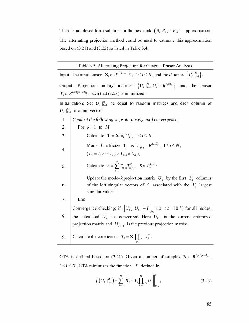
85
There is no closed form solution for the best rank– ( )1 2, , MR R RL approximation.
The alternating projection method could be used to estimate this approximation
based on (3.21) and (3.22) as listed in Table 3.4.
Table 3.5. Alternating Projection for General Tensor Analysis.
Input: The input tensor 1 2 ML L Li R × ×∈X L , 1 i N≤ ≤ , and the d–ranks { }1|Md dL =′ .
Output: Projection unitary matrices { }1| , k kL LMk k kU U R ′×
= ∈ and the tensor 1 2 ML L L
i R ′ ′ ′× × ×∈Y L , such that (3.23) is minimized.
Initialization: Set 1|Mk kU = be equal to random matrices and each column of
1|Mk kU = is a unit vector.
1. Conduct the following steps iteratively until convergence.
2. For 1k = to M
3. Calculate Ti i k kU= ×T X , 1 i N≤ ≤ ;
4. Mode–d matricize iT as ( );
k kL Li kT R ×∈ , 1 i N≤ ≤ ,
( 1 1 1k k k ML L L L L− += × × ×L );
5. Calculate ( ) ( ); ;1
NT
i k i ki
S T T=
= ∑ , k kL LS R ×+∈ .
6. Update the mode–k projection matrix kU by the first kL′ columns of the left singular vectors of S associated with the kL′ largest singular values;
7. End
8.
Convergence checking: if , 1 ,Tk t k t Fro
U U I ε− − ≤ ( 610ε −= ) for all modes,
the calculated kU has converged. Here ,k tU is the current optimized projection matrix and , 1k tU − is the previous projection matrix.
9. Calculate the core tensor 1
k
MT
i i kk
U×=
= ∏Y X .
GTA is defined based on (3.21). Given a number of samples 1 2 ML L Li R × ×∈X L ,
1 i N≤ ≤ , GTA minimizes the function f defined by
( )2
11 1
|k
MNM
k k i i ki k Fro
f U U= ×= =
= −∑ ∏X Y , (3.23)
86
where 1
k
MT
i i kk
U×=
= ∏Y X .
Based on Theorem 3.4, minimizing (3.23) is equivalent to maximizing
( )2
11 1
|k
MNM T
k k i ki k Fro
g U U= ×= =
= ∑ ∏X . (3.24)
There is no closed form solution to (3.23). A solution, listed in Table 3.5, based
on the alternating projection is similar to Table 3.3.
(Note: The algorithm is based on the fact: minimizing 2
1 1k
MN
i i ki k Fro
U×= =
−∑ ∏X Y is
equivalent to maximizing 2
1 1k
MNT
i ki k Fro
U×= =∑ ∏X .)
87
Two Dimensional Linear Discriminant Analysis
The major difference between LDA and 2DLDA is the representation of the
training samples. In LDA, the training samples are represented by vectors, while
they are represented as matrices in 2DLDA.
Suppose: the training samples are divided into C classes and the ith (1 i C≤ ≤ )
class contains Ni samples 1 2;
L Li jX R ×∈ (1 ij N≤ ≤ ). The mean matrix of all
training samples is ( ) ( );1 1 1iC N C
i j ii j iM X N
= = == ∑ ∑ ∑ and the mean matrix of the
ith class samples is ( );1iN
i i j ijM X N
== ∑ . The class structure in the high
dimensional space is defined by
( ) ( )( )
( ) ( )( )
; ;1 1
1
tr
tr ,
iNC THw i j i i j i
i j
CTH
b i i ii
D X M X M
D N M M M M
= =
=
⎛ ⎞= − −⎜ ⎟
⎝ ⎠⎛ ⎞= − −⎜ ⎟⎝ ⎠
∑∑
∑ (3.25)
The class structure in the low dimensional space is defined by
( ) ( ) ( )
( ) ( ) ( )
; ;1 1
1
tr
tr ,
iNC TL T Tw i j i i j i
i j
CTL T T
b i i ii
D U X M VV X M U
D N U M M VV M M U
= =
=
⎛ ⎞= − −⎜ ⎟
⎝ ⎠⎛ ⎞= − −⎜ ⎟⎝ ⎠
∑∑
∑ (3.26)
The 2DLDA finds two projection matrices 1 1L LU R ′×∈ and 2 2L LV R ′×∈ to
preserve the class structure of the original high dimensional space in the projected
low dimensional space by maximizing ( )( ) ( )1L Lw bD D
−. Ye et al. [173] developed
the following alternating projection method to obtain a solution of 2DLDA. The
algorithm conducts the following two steps iteratively:
Step 1: calculate U , which is the 1L′ eigenvectors of 1w bA A− associated with the
largest 1L′ eigenvalues, with the given V (it is a random matrix and each
column is a unit vector), where wA and bA are defined by
88
( ) ( )
( ) ( )
; ;1 1
1
.
iNC TTw i j i i j i
i j
CTT
b i i ii
A X M VV X M
A N M M VV M M
= =
=
= − −
= − −
∑∑
∑ (3.27)
Step 2: calculate V , which is the 2L′ eigenvectors of 1w bB B− associated with the
largest 2L′ eigenvalues, with the given U (obtained in Step 1), where wB and
bB are defined by
( ) ( )
( ) ( )
; ;1 1
1.
iNC T Tw i j i i j i
i j
CT T
b i i ii
B X M UU X M
B N M M UU M M
= =
=
= − −
= − −
∑∑
∑ (3.28)
The 2DLDA reduces the SSS problem and it is more efficient than LDA in terms
of time complexity and space complexity. The drawback of 2DLDA is the
alternating projection algorithm to obtain a solution of 2DLDA does not converge.
Therefore, the recognition accuracies are not stable over different training
iterations. For example, in the Probe A of the human gait recognition task in this
Chapter, the rank one recognition rate changes from 75% to 91% in the first 100
training iterations. This is because the projection matrices U and V do not
maximize ( )( ) ( )1L Lw bD D
−. According to steps 1 and 2, the projection matrix U is
the 1L′ eigenvectors of 1w bA A− associated with the largest 1L′ eigenvalues,
which is obtained with the given V by maximizing ( )( )1tr T T
w bU A U U A U−
while the projection matrix V is the 2L′ eigenvectors of 1w bB B− associated with
the largest 2L′ eigenvalues, which is obtained with the given U by maximizing
( )( )1tr T T
w bU B U U B U−
. The projection matrices U and V , obtained by
iteratively conducting steps 1 and 2, do not maximize ( )( ) ( )1L Lw bD D
−, because
maximizing the trace ratio between two projected matrices does not be equal to
maximizing the ratio trace between two projected matrices [103], i.e., with the
given wA and bA , the argument of maximum ( )( )1tr T T
w bU A U U A U−
by
varying U does not maximize ( ) ( )tr trT Tb wU A U U A U and with the given wB

89
and bB , the argument of maximum ( )( )1tr T T
w bV B V V B V−
by varying V does
not maximize ( ) ( )tr trT Tb wV B V V B V .
To deal with the nonconvergence problem and to accept general tensors as input
for discriminative dimension reduction, we propose GTDA in the next Section.
90
General Tensor Discriminant Analysis
Although the effectiveness and the efficiency of 2DLDA, as a preprocessing for
subsequent classification, e.g., by LDA, have been proved, 2DLDA fails to
converge in the training stage. The nonconvergence shadows the advantages of
2DLDA, because: 1) it is difficult to determine when to stop the training stage;
and 2) different numbers of training iterations will lead to different recognition
results. To solve the nonconvergence problem, we develop GTDA, which 1)
provides a converged alternating projection algorithm for training; 2) accepts
general tensors as input; 3) preserves the discriminative information for
classification; and 4) reduces the SSS problem in the subsequent classification,
e.g., by LDA. The proposed GTDA is based on the differential scatter
discriminant criterion (DCDS).
Differential Scatter Discriminant Criterion (DSDC)
The Differential Scatter Discriminant Criterion (DSDC) [39][149][143][145] is
defined by,
( ) ( )( )* arg max tr trT
T Tb w
U U IU U S U U S Uζ
== − , (3.29)
where ζ is a tuning parameter; L LU R ′×∈ ( L L′ < ) , constrained by TU U I= , is the projection matrix; and bS and wS are defined in (2.10).
According to [39] (pp. 446–447), the solution to (3.29) is equivalent to the
solution to (12) for some special ζ in (3.29). If we extract only one feature, i.e.,
U degenerates to a vector, then ( )1max w bS Sζ λ −= , which is the maximum
eigenvalue of 1w bS S− . If we want to extract L′ features simultaneously, we
estimate ζ as 1
Liiλ
′
=∑ , where 1|Li iλ ′= are the largest L′ eigenvalues of 1
w bS S− .
From [39] (pp. 446–447), it is not difficult to show that a suitable ζ in (3.29) is
( ) ( )tr trT Topt b opt opt w optU S U U S U 14. An accurate solution of (3.29) can be obtained by
14 The derivative of ( ) ( )tr trT T
b wU S U U S Uζ− with respect to U is given by b wS U S Uζ− .
To obtain a solution of (3.29), we need to set 0b wS U S Uζ− = (as we have a strict condition here,
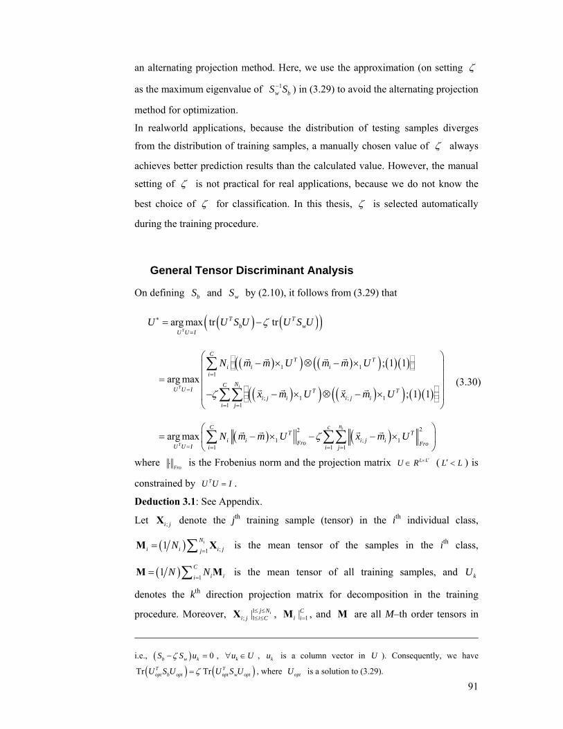
91
an alternating projection method. Here, we use the approximation (on setting ζ
as the maximum eigenvalue of 1w bS S− ) in (3.29) to avoid the alternating projection
method for optimization.
In realworld applications, because the distribution of testing samples diverges
from the distribution of training samples, a manually chosen value of ζ always
achieves better prediction results than the calculated value. However, the manual
setting of ζ is not practical for real applications, because we do not know the
best choice of ζ for classification. In this thesis, ζ is selected automatically
during the training procedure.
General Tensor Discriminant Analysis
On defining bS and wS by (2.10), it follows from (3.29) that
( ) ( )( )arg max tr trT
T Tb w
U U IU U S U U S Uζ∗
== −
( )( ) ( )( ) ( )( )
( )( ) ( )( ) ( )( )
1 11
; 1 ; 11 1
; 1 1 arg max
; 1 1iT
CT T
i i ii
NCU U I T T
i j i i j ii j
N m m U m m U
x m U x m Uζ
=
=
= =
⎛ ⎞− × ⊗ − ×⎜ ⎟⎜ ⎟=⎜ ⎟− − × ⊗ − ×⎜ ⎟⎝ ⎠
∑
∑∑
r r r r
r r r r
( ) ( ) 22
1 ; 11 1 1
arg maxi
T
nC cT T
i i i j iFro FroU U I i i jN m m U x m Uζ
= = = =
⎛ ⎞= − × − − ×⎜ ⎟
⎝ ⎠∑ ∑∑r r r r
(3.30)
where Fro
⋅ is the Frobenius norm and the projection matrix L LU R ′×∈ ( L L′ < ) is
constrained by TU U I= .
Deduction 3.1: See Appendix.
Let ;i jX denote the jth training sample (tensor) in the ith individual class,
( ) ;11 iN
i i i jjN
== ∑M X is the mean tensor of the samples in the ith class,
( ) 11 C
i iiN N
== ∑M M is the mean tensor of all training samples, and kU
denotes the kth direction projection matrix for decomposition in the training
procedure. Moreover, 1; 1| ij N
i j i C≤ ≤≤ ≤X , 1|Ci i=M , and M are all M–th order tensors in
i.e., ( ) 0b w kS S uζ− = , ku U∀ ∈ , ku is a column vector in U ). Consequently, we have
( ) ( )Tr TrT Topt b opt opt w optU S U U S Uζ= , where optU is a solution to (3.29).
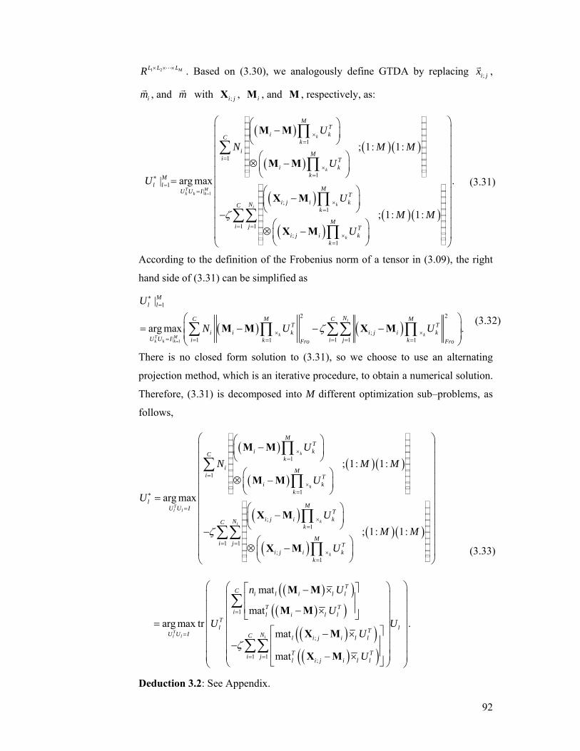
92
1 2 ML L LR × × ×L . Based on (3.30), we analogously define GTDA by replacing ;i jxr ,
imr , and mr with ;i jX , iM , and M , respectively, as:
( )
( )( )( )
( )
( )( )( )
1
1
1
11
|
;1
1 1;
1
; 1: 1:
| arg max
; 1: 1:
k
k
T Mk k k
ki
k
MT
i kCk
i Mi T
i kkM
l l MU U I Ti j i kNC
k
Mi j T
i j i kk
UN M M
UU
UM M
Uζ
=
×=
=×
=∗=
=
×=
= =×
=
⎛ ⎛ ⎞−⎜ ⎜ ⎟
⎝ ⎠⎜⎜ ⎛ ⎞⎜ ⊗ −⎜ ⎟⎜ ⎝ ⎠
= ⎜⎛ ⎞⎜ −⎜ ⎟⎜ ⎝ ⎠⎜−⎛ ⎞
⊗ −⎜ ⎟⎝ ⎠⎝
∏∑
∏
∏∑∑
∏
M M
M M
X M
X M
⎞⎟⎟⎟⎟⎟⎟⎟⎟⎟
⎜ ⎟⎜ ⎟
⎠
. (3.31)
According to the definition of the Frobenius norm of a tensor in (3.09), the right
hand side of (3.31) can be simplified as
( ) ( )1
1
2 2
;| 1 1 11 1
|
arg max .i
k kT Mk k k
Ml l
NM MC CT T
i i k i j i kU U I i i jk kFro Fro
U
N U Uζ=
∗=
× ×= = = == =
⎛ ⎞= − − −⎜ ⎟⎜ ⎟
⎝ ⎠∑ ∑∑∏ ∏M M X M
(3.32)
There is no closed form solution to (3.31), so we choose to use an alternating
projection method, which is an iterative procedure, to obtain a numerical solution.
Therefore, (3.31) is decomposed into M different optimization sub–problems, as
follows,
( )
( )( )( )
( )
( )( )( )
1
1
1
;1
1 1;
1
; 1: 1:
arg max
; 1: 1:
k
k
Tl l
ki
k
MT
i kCk
i Mi T
i kk
l MU U I Ti j i kNC
k
Mi j T
i j i kk
UN M M
UU
UM M
Uζ
×=
=×
=∗
=
×=
= =×
=
⎛ ⎞⎛ ⎞−⎜ ⎟⎜ ⎟
⎝ ⎠⎜ ⎟⎜ ⎟⎛ ⎞⎜ ⎟⊗ −⎜ ⎟⎜ ⎟⎝ ⎠
= ⎜ ⎟⎛ ⎞⎜ −⎜ ⎟⎜ ⎝ ⎠⎜−
⎜ ⎛ ⎞⊗ −⎜ ⎜ ⎟⎝ ⎠⎝ ⎠
∏∑
∏
∏∑∑
∏
M M
M M
X M
X M
⎟⎟⎟⎟⎟
( )( )( )( )
( )( )( )( )
1
;
1 1 ;
mat
mat arg max tr
mat
mat
Tl l i
TC i l i l l
T Ti l i l l
Tl lTU U I NC l i j i l l
T Ti j l i j i l l
n U
UU U
U
Uζ
=
=
= =
⎛ ⎞⎛ ⎞⎡ ⎤− ×⎜ ⎟⎜ ⎟⎢ ⎥⎜ ⎟⎜ ⎟⎢ ⎥− ×⎣ ⎦⎜ ⎟⎜ ⎟= ⎜ ⎟⎜ ⎟⎡ ⎤− ×⎜ ⎟⎜ ⎟⎢ ⎥−⎜ ⎟⎜ ⎟⎢ ⎥⎜ − × ⎟⎜ ⎟⎣ ⎦⎝ ⎠⎝ ⎠
∑
∑∑
M M
M M
X M
X M
.
(3.33)
Deduction 3.2: See Appendix.
93
To simplify (3.33), we define
( )( ) ( )( )1
mat matC
T T Tl i l i l l l i l l
iB N U U
=
⎡ ⎤= − × − ×⎣ ⎦∑ M M M M , (3.34)
and
( )( ) ( )( ); ;1 1
mat matiNC
T T Tl l i j i l l l i j i l l
i jW U U
= =
⎡ ⎤= − × − ×⎣ ⎦∑∑ X M X M . (3.35)
Therefore, (3.33) is simplified as,
( )( )1
1|
* | arg max trT Ml l l
M Tl l l l l l
U U IU U B W Uζ
=
==
= − . (3.36)
As pointed out in 0, ζ is the tuning parameter.
Table 3.6 lists the alternating projection method based optimization procedure for
GTDA with the given tuning parameter ζ to simplify the proof of the
convergence theorem. Later, we describe how to determine the tuning parameter
ζ and the dimension 1 2 ML L L′ ′ ′× ×L of the output tensors automatically. The
key steps in the alternating projection procedure are Steps 3–5, which involve
finding the lth mode projection matrix ,l tU in the tth iteration using 1, 1|lk t kU −
=
obtained in the tth iteration and , 1 1|Mk t k lU − = + obtained in the ( 1t − )th iteration. In
Steps 3 and 4, we obtain the between class scatter matrix , 1l tB − and the within
class scatter matrix , 1l tW − with 1, 1|lk t kU −
= obtained in the tth iteration and
, 1 1|Mk t k lU − = + obtained in the ( 1t − )th iteration. The singular value decomposition
(SVD) of , 1 , 1l t l tB Wζ− −− is obtained and , 1l tU − is updated using the eigenvectors
of , 1 , 1l t l tB Wζ− −− , which correspond to the largest eigenvalues of , 1 , 1l t l tB Wζ− −− .
According to the algorithm described in Table 3.6, we can obtain a solution
1| k kL LMk kU R ′×
= ∈ ( k kL L′ < ) by an iterative way. For GTDA, we use the projected
tensor 1
k
MTk
k
U×=
= ∏Y X to represent the original general tensor X . Unlike
2DLDA [173], the alternating projection method based optimization procedure for
GTDA converges, as proved in Theorem 3.5.
Theorem 3.5 The alternating projection method based optimization procedure for
GTDA converges.
Proof: See Appendix.
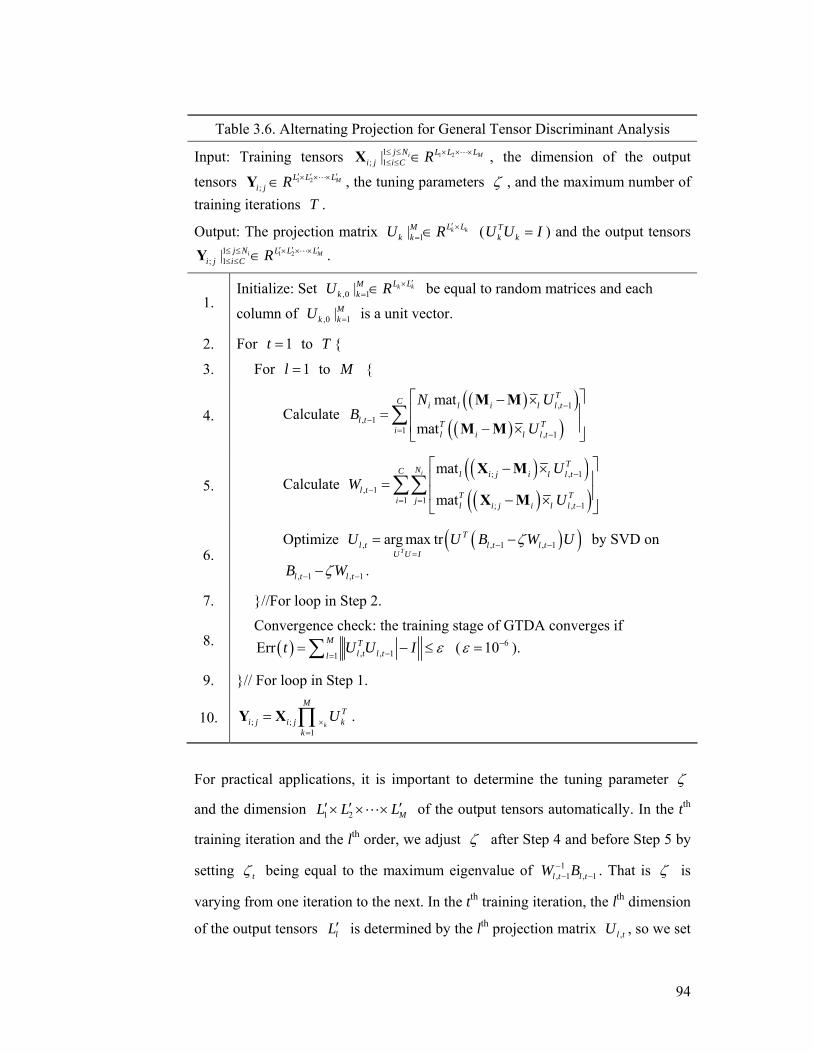
94
Table 3.6. Alternating Projection for General Tensor Discriminant Analysis
Input: Training tensors 1 21; 1| i Mj N L L L
i j i C R≤ ≤ × × ×≤ ≤ ∈X L , the dimension of the output
tensors 1 2;
ML L Li j R ′ ′ ′× × ×∈Y L , the tuning parameters ζ , and the maximum number of
training iterations T .
Output: The projection matrix 1| k kL LMk kU R ′ ×
= ∈ ( Tk kU U I= ) and the output tensors
1 21; 1| i Mj N L L L
i j i C R ′ ′ ′≤ ≤ × × ×≤ ≤ ∈Y L .
1. Initialize: Set ,0 1| k kL LM
k kU R ′×= ∈ be equal to random matrices and each
column of ,0 1|Mk kU = is a unit vector.
2. For 1t = to T {
3. For 1l = to M {
4. Calculate ( )( )
( )( ), 1
, 11 , 1
mat
mat
TC i l i l l t
l t T Ti l i l l t
N UB
U
−
−= −
⎡ ⎤− ×⎢ ⎥=⎢ ⎥− ×⎣ ⎦
∑M M
M M
5. Calculate ( )( )( )( )
; , 1
, 11 1 ; , 1
mat
mat
iT
NC l i j i l l t
l t T Ti j l i j i l l t
UW
U
−
−= =
−
⎡ ⎤− ×⎢ ⎥=⎢ ⎥− ×⎣ ⎦
∑∑X M
X M
6. Optimize ( )( ), , 1 , 1arg max tr
T
Tl t l t l t
U U IU U B W Uζ− −
== − by SVD on
, 1 , 1l t l tB Wζ− −− .
7. }//For loop in Step 2.
8. Convergence check: the training stage of GTDA converges if
( ) , , 11Err M T
l t l tlt U U I ε−== − ≤∑ ( 610ε −= ).
9. }// For loop in Step 1.
10. ; ;1
k
MT
i j i j kk
U×=
= ∏Y X .
For practical applications, it is important to determine the tuning parameter ζ
and the dimension 1 2 ML L L′ ′ ′× × ×L of the output tensors automatically. In the tth
training iteration and the lth order, we adjust ζ after Step 4 and before Step 5 by
setting tζ being equal to the maximum eigenvalue of 1, 1 , 1l t l tW B−− − . That is ζ is
varying from one iteration to the next. In the tth training iteration, the lth dimension
of the output tensors lL′ is determined by the lth projection matrix ,l tU , so we set
95
a threshold value δ to automatically determine lL′ according to the following
inequality:
,1, ,1, ,2,
, , , ,1 1
1, , , ,1 1
, , , ,1 1
, ,1
, ,1
1,
l l
l l
l l
l
l
l t l t l tL L
l j t l j tj j
L Ll i t l i ti i
L Ll j t l j tj j
Ll i ti
Ll j tj
λ λ λ
λ λ
λ λδ
λ λ
λ
λ
= =
′ ′+
= =
= =
=
=
+< <
< ≤ < <
< =
∑ ∑∑ ∑∑ ∑
∑∑
L
L . (3.37)
where , ,l i tλ is the ith eigenvalue of , 1 , 1l t t l tB Wζ− −− and , , , ,l i t l j tλ λ≥ if i j< .
Therefore, there is only one parameter, the threshold value δ , which needs to be
tuned for recognition tasks. Without this method as shown in (3.37), we have to
tune 1M + parameters, comprising of one parameter for each order of the M–th
order tensors and ζ in (3.36). This multiparameter tuning is too time consuming
when M is large.
Computational Complexity
The time complexity of LDA is ( )3
1
Mii
O L=
⎛ ⎞⎜ ⎟⎝ ⎠∏ in the training stage, where
training samples X belong to 1 2 ML L LR × × ×L . The time complexity of the
alternating projection method based optimization procedure of GTDA is
( )31
Mii
O T L=∑ , where T is the number of iterations required for GTDA to
converge. The space complexity of LDA is ( )2
1
Mii
O L=
⎛ ⎞⎜ ⎟⎝ ⎠∏ in the training stage.
The space complexity of the alternating projection method based optimization
procedure of GTDA is ( )21
Mii
O L=∑ .
96
Manifold Learning using Tensor Representations
The proposed GTDA can also be extended for manifold learning [13], which has
become popular in machine learning. Manifold learning is based on geometrical
assumptions, i.e., a data set approximately lies in a low dimensional manifold
embedded in the original high dimensional feature space. Recently, a large
number of algorithms have been developed based on different criteria. For
example, ISOMAP [155] finds the low dimensional representation for data by
preserving the geodesic distances of data pairs in the original high dimensional
space. Locally linear embedding (LLE) [124][127] produces the low dimensional
representation for locally sufficient reconstruction, i.e., a sample is reconstructed
from its neighborhood samples. Laplacian Eigenmap (LE) [5][6]reduces the data
dimension by preserving the locality character of the samples. Recently, Bengio et
al. [8] unified a number of manifold learning algorithms together and developed
the out of sample extension. Yan et al. [172] developed another framework,
named the graph embedding framework (GEF). GEF finds the projection matrix L LU R ′×∈ ( L L′ < ) to map the original high dimensional samples Lx R∈
r to the
low dimensional space LR ′ through a linear projection, i.e., Ty U x=r r and
Ly R ′∈r . The objective function of GEF is defined by
( )( )
( )
2
1 1
2
1 1
N NT
ij i j Froi jN N
Tij i j Froi j
b U x xF U
s U x x
= =
= =
−=
−
∑∑
∑∑
r r
r r, (3.38)
where ijs and ijb are predefined weighting factors and N is the number of
training samples. By varying ijs and ijb , different dimension reduction
algorithms can be obtained, e.g., LLE, ISOMAP, and LDA. The linear projection
matrix L LU R ′×∈ is obtained by maximizing ( )F U subject to the constraint
TU U I= . To extend GEF to accept general tensors as input, we reformulate
(3.38) as
97
( ) ( ) ( )
( ) ( )
( ) ( )
( )( )( )( )( )
( )( )
2 2
1 1 1 1
2
1 1
2
11 1
1
1
; 1 1
n n n nT T
ij i j ij i jFro Froi j i j
n nT
ij ij i j Froi j
n nT
ij ij i j Froi j
Ti j
ij ij Tj i j
G U b U x x s U x x
b s U x x
b s x x U
x x Ub s
x x U
ζ
ζ
ζ
ζ
= = = =
= =
= =
= − − −
= − −
= − − ×
− ×= −
⊗ − ×
∑∑ ∑∑
∑∑
∑∑
r r r r
r r
r r
r r
r r1 1
,n n
i= =∑∑
(3.39)
where ζ is a tuning parameter and the linear projection matrix U is obtained
by maximizing ( )G U constrained by TU U I= .
Based on (3.33), we analogously define tensorized GEF by replacing ixr with
iX as
( ) ( )( )
( )( )( )1
11 1
1
| ; 1: 1: ,k
k
MT
i j kN NkM
k k ij ij Mi j T
i j kk
UH U b s M M
Uζ
×=
== =
×=
⎛ ⎞−⎜ ⎟
⎝ ⎠= −⎛ ⎞
⊗ −⎜ ⎟⎝ ⎠
∏∑∑
∏
X X
X X (3.40)
where ζ is a tuning parameter and a series of linear projection matrices 1|Mk kU =
is obtained by maximizing ( )1|Mk kH U = constrained by Tk kU U I= for
1 k M≤ ≤ . According to (3.09), the tensorized GEF can be defined as
( )
( ) ( )
1
1
1 1|
2
| 1 1 1
| arg max |
arg max .
T Mk k k
kT Mk k k
M Mk k k k
U U I
MN NT
ij ij i j kU U I i j k Fro
U H U
b s Uζ
=
=
∗= =
=
×= = = =
=
⎛ ⎞= − −⎜ ⎟⎜ ⎟
⎝ ⎠∑∑ ∏X X
(3.41)
Similar to GTDA, there is no closed form solution. Therefore, (3.41) is
decomposed into M different optimization sub–problems, as follows,
( )( )
( )( )( )
( )( )( )( )( )
1
1 1
1
1 1
arg max ; 1: 1:
mat arg max tr
mat
k
Tk k
k
Tk k
MT
i j kN Nk
k ij ij MU U I i j Ti j k
k
TN N k i j k kT
k ij ij T TU U I i j k i j k k
UU b s M M
U
UU b s
U
ζ
ζ
×=∗
= = =×
=
= = =
⎛ ⎞⎛ ⎞−⎜ ⎟⎜ ⎟
⎝ ⎠⎜ ⎟= −⎜ ⎟⎛ ⎞⎜ ⎟⊗ −⎜ ⎟⎜ ⎟⎝ ⎠⎝ ⎠
⎛ ⎡ ⎤− ×⎜ ⎢ ⎥= −
⎢ ⎥− ×⎣ ⎦⎝
∏∑∑
∏
∑∑
X X
X X
X X
X X.kU
⎛ ⎞⎞⎜ ⎟⎟⎜ ⎟⎜ ⎟⎜ ⎟⎜ ⎟⎠⎝ ⎠
(3.42)

98
With (3.42), a solution to the tensorized GEF can be obtained iteratively by the
alternating projection method.
99
GTDA for Human Gait Recognition
A straightforward application of LDA to human gait recognition leads to poor
results because of the SSS problem. For this reason, principal component analysis
(PCA) [30] is conducted as a preprocessing step to reduce the SSS problem.
Unfortunately, some discriminative information is discarded by PCA.
In this Section, we apply the proposed GTDA to reduce the SSS problem in LDA
for appearance based human gait recognition [126]. Appearance [83] is the basic
stage of visual information representation and reflects the walking manner
[45][91]. In the following, we use the averaged gait image [45][91] as the
appearance model. As a representation method, the effectiveness of the averaged
gait image based recognition has been proved in [45][46][91][92].
The averaged gait image is decomposed by Gabor functions [25][26][101] and we
combine the decomposed images to give new representations for recognition.
There are three major reasons for introducing the Gabor based representation for
the averaged gait image based recognition: 1) human brains seem to have a
special function to process information in multi–resolution levels [25][26][101];
2) it is supposed that Gabor functions are similar to the receptive field profiles in
the mammalian cortical simple cells [25][101]; and 3) Gabor function based
representations have been successfully employed in many computer vision
applications, such as face recognition [87][88][89] and texture analysis [32].
Although Gabor function based representations are effective for object
recognition [25][26] and image understanding, the computational cost of the
representation is high. Therefore, three variant methods for representation are
introduced to utilize Gabor functions to reduce the computational cost in
calculating the representation and in training subsequent feature selection
algorithms by partially or fully summing over Gabor functions. The sum operation
reduces the number of functions, used for decomposing the averaged gait images.
These methods are: 1) the sum over directions of Gabor functions based
representation (GaborD), 2) the sum over scales of Gabor functions based
representation (GaborS), and 3) the sum over both scales and directions of Gabor
functions based representation (GaborSD).
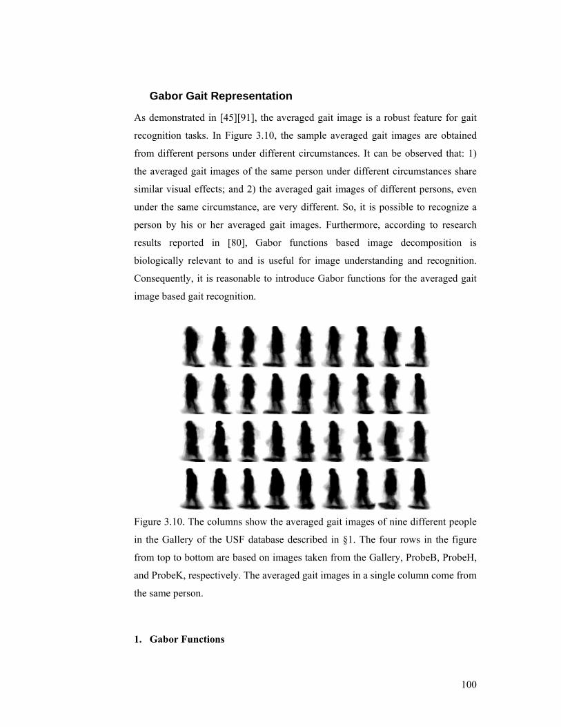
100
Gabor Gait Representation
As demonstrated in [45][91], the averaged gait image is a robust feature for gait
recognition tasks. In Figure 3.10, the sample averaged gait images are obtained
from different persons under different circumstances. It can be observed that: 1)
the averaged gait images of the same person under different circumstances share
similar visual effects; and 2) the averaged gait images of different persons, even
under the same circumstance, are very different. So, it is possible to recognize a
person by his or her averaged gait images. Furthermore, according to research
results reported in [80], Gabor functions based image decomposition is
biologically relevant to and is useful for image understanding and recognition.
Consequently, it is reasonable to introduce Gabor functions for the averaged gait
image based gait recognition.
Figure 3.10. The columns show the averaged gait images of nine different people
in the Gallery of the USF database described in §1. The four rows in the figure
from top to bottom are based on images taken from the Gallery, ProbeB, ProbeH,
and ProbeK, respectively. The averaged gait images in a single column come from
the same person.
1. Gabor Functions
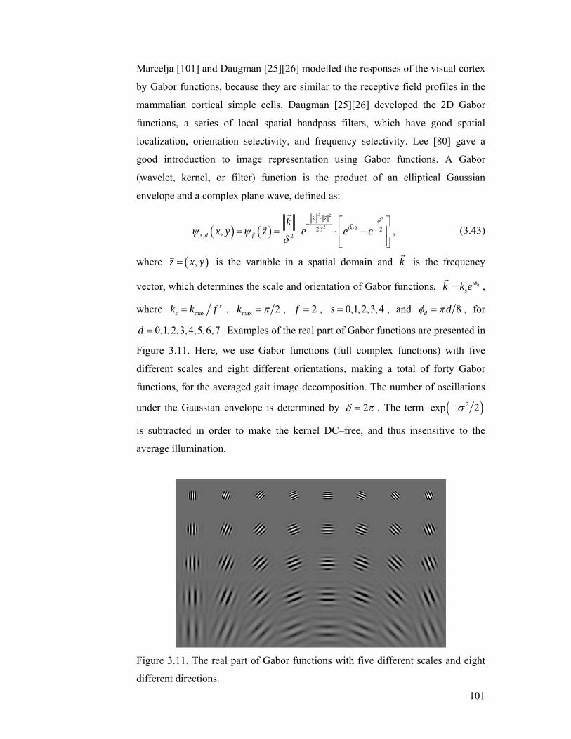
101
Marcelja [101] and Daugman [25][26] modelled the responses of the visual cortex
by Gabor functions, because they are similar to the receptive field profiles in the
mammalian cortical simple cells. Daugman [25][26] developed the 2D Gabor
functions, a series of local spatial bandpass filters, which have good spatial
localization, orientation selectivity, and frequency selectivity. Lee [80] gave a
good introduction to image representation using Gabor functions. A Gabor
(wavelet, kernel, or filter) function is the product of an elliptical Gaussian
envelope and a complex plane wave, defined as:
( ) ( )2 2
2
22 2, 2,
k zik z
s d k
kx y z e e e
δδψ ψ
δ
⋅− −⋅
⎡ ⎤= = ⋅ ⋅ −⎢ ⎥
⎢ ⎥⎣ ⎦
r r
r rr
rr , (3.43)
where ( ),z x y=r is the variable in a spatial domain and kr
is the frequency
vector, which determines the scale and orientation of Gabor functions, disk k e φ=
r,
where maxs
sk k f= , max 2k π= , 2f = , 0,1,2,3,4s = , and 8d dφ π= , for
0,1,2,3,4,5,6,7d = . Examples of the real part of Gabor functions are presented in
Figure 3.11. Here, we use Gabor functions (full complex functions) with five
different scales and eight different orientations, making a total of forty Gabor
functions, for the averaged gait image decomposition. The number of oscillations
under the Gaussian envelope is determined by 2δ π= . The term ( )2exp 2σ−
is subtracted in order to make the kernel DC–free, and thus insensitive to the
average illumination.
Figure 3.11. The real part of Gabor functions with five different scales and eight
different directions.
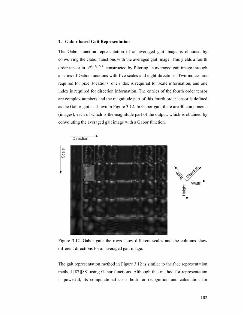
102
2. Gabor based Gait Representation
The Gabor function representation of an averaged gait image is obtained by
convolving the Gabor functions with the averaged gait image. This yields a fourth
order tensor in 1 2 5 8L LR × × × constructed by filtering an averaged gait image through
a series of Gabor functions with five scales and eight directions. Two indices are
required for pixel locations: one index is required for scale information, and one
index is required for direction information. The entries of the fourth order tensor
are complex numbers and the magnitude part of this fourth order tensor is defined
as the Gabor gait as shown in Figure 3.12. In Gabor gait, there are 40 components
(images), each of which is the magnitude part of the output, which is obtained by
convoluting the averaged gait image with a Gabor function.
Figure 3.12. Gabor gait: the rows show different scales and the columns show
different directions for an averaged gait image.
The gait representation method in Figure 3.12 is similar to the face representation
method [87][88] using Gabor functions. Although this method for representation
is powerful, its computational costs both for recognition and calculation for
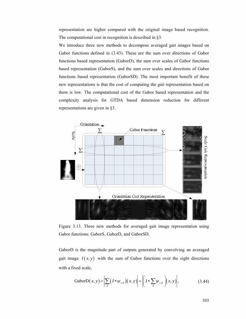
103
representation are higher compared with the original image based recognition.
The computational cost in recognition is described in §3.
We introduce three new methods to decompose averaged gait images based on
Gabor functions defined in (3.43). These are the sum over directions of Gabor
functions based representation (GaborD), the sum over scales of Gabor functions
based representation (GaborS), and the sum over scales and directions of Gabor
functions based representation (GaborSD). The most important benefit of these
new representations is that the cost of computing the gait representation based on
them is low. The computational cost of the Gabor based representation and the
complexity analysis for GTDA based dimension reduction for different
representations are given in §3.
∑∑
∑
Figure 3.13. Three new methods for averaged gait image representation using
Gabor functions: GaborS, GaborD, and GaborSD.
GaborD is the magnitude part of outputs generated by convolving an averaged
gait image ( ),I x y with the sum of Gabor functions over the eight directions
with a fixed scale,
( ) ( )( ) ( ), ,GaborD , , ,s d s dd d
x y I x y I x yψ ψ⎛ ⎞= ∗ = ∗⎜ ⎟⎝ ⎠
∑ ∑ , (3.44)
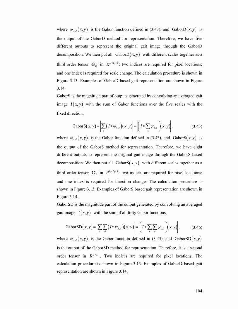
104
where ( ), ,s d x yψ is the Gabor function defined in (3.43); and ( )GaborD ,x y is
the output of the GaborD method for representation. Therefore, we have five
different outputs to represent the original gait image through the GaborD
decomposition. We then put all ( )GaborD ,x y with different scales together as a
third order tensor DG in 1 2 5L LR × × : two indices are required for pixel locations;
and one index is required for scale change. The calculation procedure is shown in
Figure 3.13. Examples of GaborD based gait representation are shown in Figure
3.14.
GaborS is the magnitude part of outputs generated by convolving an averaged gait
image ( ),I x y with the sum of Gabor functions over the five scales with the
fixed direction,
( ) ( )( ) ( ), ,GaborS , , ,s d s ds s
x y I x y I x yψ ψ⎛ ⎞= ∗ = ∗⎜ ⎟⎝ ⎠
∑ ∑ , (3.45)
where ( ), ,s d x yψ is the Gabor function defined in (3.43), and ( )GaborS ,x y is
the output of the GaborS method for representation. Therefore, we have eight
different outputs to represent the original gait image through the GaborS based
decomposition. We then put all ( )GaborS ,x y with different scales together as a
third order tensor SG in 1 2 8L LR × × : two indices are required for pixel locations;
and one index is required for direction change. The calculation procedure is
shown in Figure 3.13. Examples of GaborS based gait representation are shown in
Figure 3.14.
GaborSD is the magnitude part of the output generated by convolving an averaged
gait image ( ),I x y with the sum of all forty Gabor functions,
( ) ( )( ) ( ), ,GaborSD , , ,s d s ds d s d
x y I x y I x yψ ψ⎛ ⎞= ∗ = ∗⎜ ⎟⎝ ⎠
∑∑ ∑∑ , (3.46)
where ( ), ,s d x yψ is the Gabor function defined in (3.43), and ( )GaborSD ,x y
is the output of the GaborSD method for representation. Therefore, it is a second
order tensor in 1 2L LR × . Two indices are required for pixel locations. The
calculation procedure is shown in Figure 3.13. Examples of GaborD based gait
representation are shown in Figure 3.14.
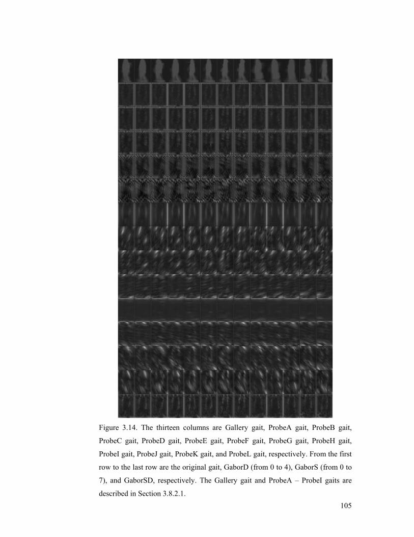
105
Figure 3.14. The thirteen columns are Gallery gait, ProbeA gait, ProbeB gait,
ProbeC gait, ProbeD gait, ProbeE gait, ProbeF gait, ProbeG gait, ProbeH gait,
ProbeI gait, ProbeJ gait, ProbeK gait, and ProbeL gait, respectively. From the first
row to the last row are the original gait, GaborD (from 0 to 4), GaborS (from 0 to
7), and GaborSD, respectively. The Gallery gait and ProbeA – ProbeI gaits are
described in Section 3.8.2.1.
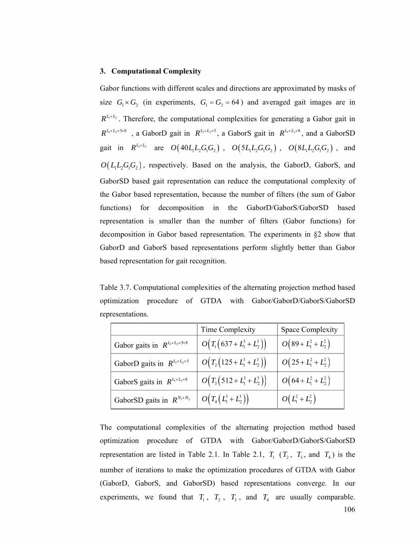
106
3. Computational Complexity
Gabor functions with different scales and directions are approximated by masks of
size 1 2G G× (in experiments, 1 2 64G G= = ) and averaged gait images are in
1 2L LR × . Therefore, the computational complexities for generating a Gabor gait in 1 2 5 8L LR × × × , a GaborD gait in 1 2 5L LR × × , a GaborS gait in 1 2 8L LR × × , and a GaborSD
gait in 1 2L LR × are ( )1 2 1 240O L L G G , ( )1 2 1 25O L L G G , ( )1 2 1 28O L L G G , and
( )1 2 1 2O L L G G , respectively. Based on the analysis, the GaborD, GaborS, and
GaborSD based gait representation can reduce the computational complexity of
the Gabor based representation, because the number of filters (the sum of Gabor
functions) for decomposition in the GaborD/GaborS/GaborSD based
representation is smaller than the number of filters (Gabor functions) for
decomposition in Gabor based representation. The experiments in §2 show that
GaborD and GaborS based representations perform slightly better than Gabor
based representation for gait recognition.
Table 3.7. Computational complexities of the alternating projection method based
optimization procedure of GTDA with Gabor/GaborD/GaborS/GaborSD
representations.
Time Complexity Space Complexity
Gabor gaits in 1 2 5 8L LR × × × ( )( )3 31 1 2637O T L L+ + ( )2 2
1 289O L L+ +
GaborD gaits in 1 2 5L LR × × ( )( )3 32 1 2125O T L L+ + ( )2 2
1 225O L L+ +
GaborS gaits in 1 2 8L LR × × ( )( )3 33 1 2512O T L L+ + ( )2 2
1 264O L L+ +
GaborSD gaits in 1 2N NR × ( )( )3 34 1 2O T L L+ ( )2 2
1 2O L L+
The computational complexities of the alternating projection method based
optimization procedure of GTDA with Gabor/GaborD/GaborS/GaborSD
representation are listed in Table 2.1. In Table 2.1, 1T ( 2T , 3T , and 4T ) is the
number of iterations to make the optimization procedures of GTDA with Gabor
(GaborD, GaborS, and GaborSD) based representations converge. In our
experiments, we found that 1T , 2T , 3T , and 4T are usually comparable.
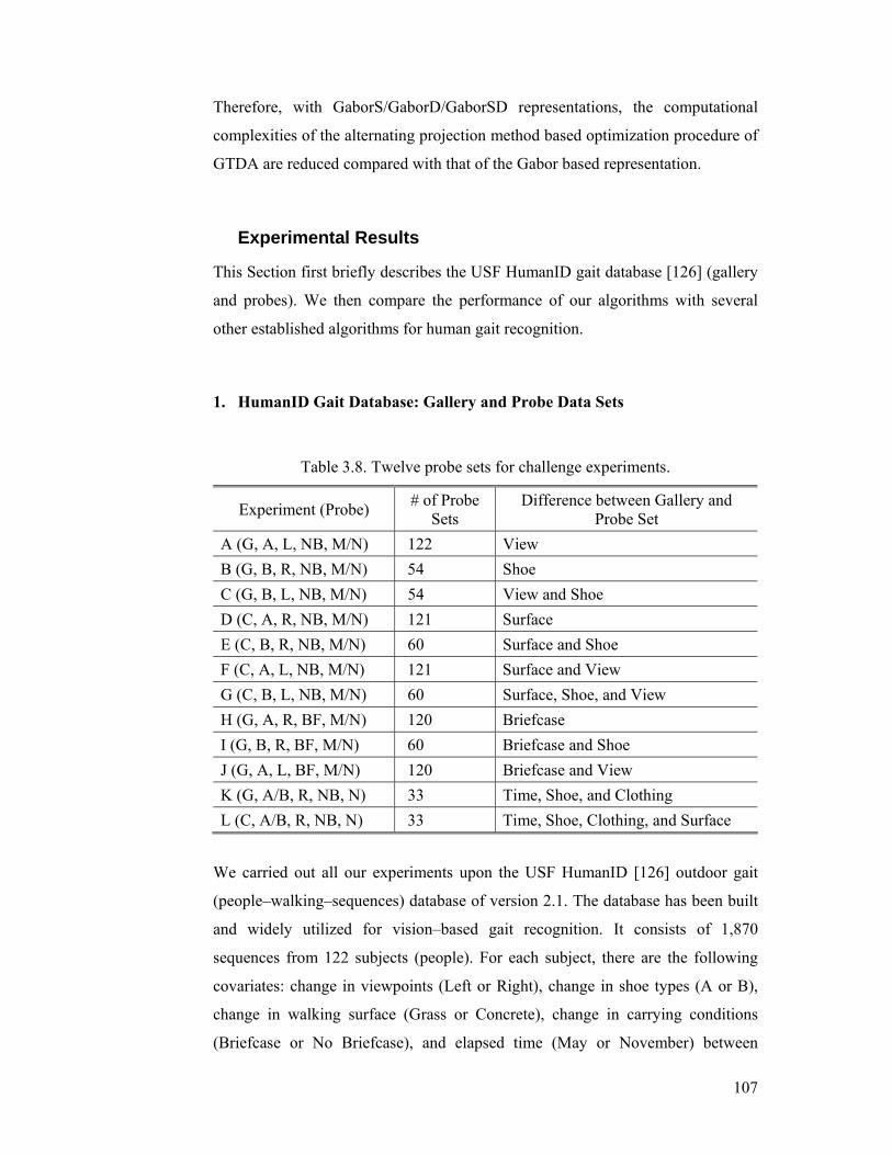
107
Therefore, with GaborS/GaborD/GaborSD representations, the computational
complexities of the alternating projection method based optimization procedure of
GTDA are reduced compared with that of the Gabor based representation.
Experimental Results
This Section first briefly describes the USF HumanID gait database [126] (gallery
and probes). We then compare the performance of our algorithms with several
other established algorithms for human gait recognition.
1. HumanID Gait Database: Gallery and Probe Data Sets
Table 3.8. Twelve probe sets for challenge experiments.
Experiment (Probe) # of Probe Sets
Difference between Gallery and Probe Set
A (G, A, L, NB, M/N) 122 View B (G, B, R, NB, M/N) 54 Shoe C (G, B, L, NB, M/N) 54 View and Shoe D (C, A, R, NB, M/N) 121 Surface E (C, B, R, NB, M/N) 60 Surface and Shoe F (C, A, L, NB, M/N) 121 Surface and View G (C, B, L, NB, M/N) 60 Surface, Shoe, and View H (G, A, R, BF, M/N) 120 Briefcase I (G, B, R, BF, M/N) 60 Briefcase and Shoe J (G, A, L, BF, M/N) 120 Briefcase and View K (G, A/B, R, NB, N) 33 Time, Shoe, and Clothing L (C, A/B, R, NB, N) 33 Time, Shoe, Clothing, and Surface
We carried out all our experiments upon the USF HumanID [126] outdoor gait
(people–walking–sequences) database of version 2.1. The database has been built
and widely utilized for vision–based gait recognition. It consists of 1,870
sequences from 122 subjects (people). For each subject, there are the following
covariates: change in viewpoints (Left or Right), change in shoe types (A or B),
change in walking surface (Grass or Concrete), change in carrying conditions
(Briefcase or No Briefcase), and elapsed time (May or November) between
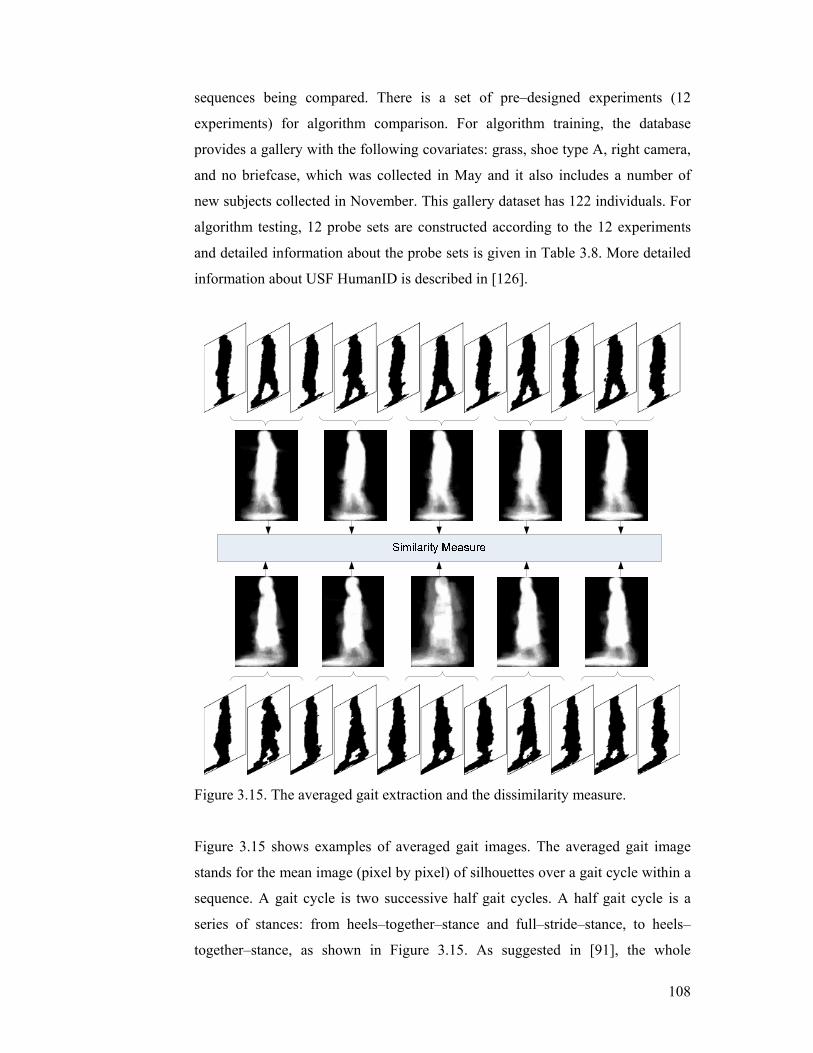
108
sequences being compared. There is a set of pre–designed experiments (12
experiments) for algorithm comparison. For algorithm training, the database
provides a gallery with the following covariates: grass, shoe type A, right camera,
and no briefcase, which was collected in May and it also includes a number of
new subjects collected in November. This gallery dataset has 122 individuals. For
algorithm testing, 12 probe sets are constructed according to the 12 experiments
and detailed information about the probe sets is given in Table 3.8. More detailed
information about USF HumanID is described in [126].
Figure 3.15. The averaged gait extraction and the dissimilarity measure.
Figure 3.15 shows examples of averaged gait images. The averaged gait image
stands for the mean image (pixel by pixel) of silhouettes over a gait cycle within a
sequence. A gait cycle is two successive half gait cycles. A half gait cycle is a
series of stances: from heels–together–stance and full–stride–stance, to heels–
together–stance, as shown in Figure 3.15. As suggested in [91], the whole
109
sequence is partitioned into a series of sub–sequences according to the gait period
(a cycle) length GaitN . Then the binary images within one cycle (a sub–sequence)
are averaged to acquire a set of averaged silhouette images iAS , i.e.
( )( )1 1
/1|
GaitGait
Gait
k i NT N
i i Gaitk iN
AS S k N= + −
⎢ ⎥⎣ ⎦=
=
⎛ ⎞= ⎜ ⎟⎜ ⎟⎝ ⎠
∑ . (3.47)
The averaged gait representation is robust against any errors in individual frames,
so we choose the averaged gait image to represent a gait cycle. One sequence
yields several averaged gait images and the number of averaged gait images
depends on the number of gait cycles in this sequence. In the following
experiments, averaged gait images are utilized as the original data for the gait
recognition problem. Some further averaged gait images from the gallery set are
also shown in Figure 3.10, which demonstrate that averaged gait images can be
used for gait recognition, because different people have different averaged gait
images.
The dissimilarity measure in gait recognition is the same as in [91]. The distance
between the gallery sequence and the probe sequence is
( )( ) ( )( )1 1
Dist ,
Median min ,p G
Method MethodP G
N N Method Methodi j P G
AS AS
AS i AS j= == − (3.48)
where ( ) 1| PNMethodP iAS i = is the ith projected AS in the probe data and
( ) 1| GNMethodG jAS j = is the jth projected AS in the gallery. The right hand side of (3.48)
is the median of the Euclidean distances between averaged silhouettes from the
probe and the gallery. It is suggested as a suitable measure for gait recognition by
Liu and Sarkar in [91].
There are only two parameters in all proposed methods, one for GTDA and the
other for LDA. In detail, one parameter is the threshold value δ for GTDA as
described in (3.37). In all experiments, we vary δ from 0.85 to 0.995 with a step
0.005. In 2DLDA, a similar strategy is used, i.e., δ is used to determine the
dimensions of the projected subspace in each order. The other parameter is the
number of selected dimensions in LDA. In all experiments relevant to LDA, we
vary the number of dimensions from 1 to 121 with a step 1. To speed up all
experiments, we down sample the original averaged gait images from 128 88× to
64 44× in all proposed methods. These are indicated by the note “H” in Table 3.9
110
and Table 3.10. We also show some experimental results based on the original
averaged gait images with the size 128 88× .
To examine the effectiveness of the automatic selection of ζ for GTDA based
recognition defined in (3.31), we also manually tune the parameters to achieve
further improvement by changing the selected dimensions for each mode and the
Lagrange multiplier ζ defined in (3.36). This is indicated by the note “M” in
Table 3.9 and Table 3.10. Although manually tuning parameters improves the
performance, it is time consuming. Moreover, the improvement is limited, so the
automatic parameter selection used in this Chapter is enough for applications.
2. Performance Evaluation
Sarkar et al. [126] evaluated the performance of the baseline algorithm on the
HumanID challenge database using the rank one/five recognition rates: 1) the rank
one recognition rate is the percentage of the number of the correct subjects in the
first place of a list of matches obtained by an algorithm and 2) the rank five
recognition rate is the percentage of the number of the correct subjects in any of
the first five places of a list of matches obtained by an algorithm. Twelve
experiments have been designed, namely experiment A to experiment L, as shown
in Table 3.8. The baseline algorithm reports the rank one recognition rates of the
twelve experiments with increasing difficulty from 78% as the easiest to 3% as
the hardest by examining the effects of the introduced five covariates (under
different combinations).
Table 3.9 and Table 3.10 report all experiments, which compare the proposed
algorithms with the existing algorithms. The item “Avg” in Table 3.9 and Table
3.10 means the averaged recognition rates of all probes (A–L), i.e., the ratio of
correctly recognized subjects to the total number of subjects in all probes. The
columns labeled A to L are exactly the same tasks as in the baseline algorithm. In
both tables, the first rows give the performance of Baseline [126], HMM [66],
IMED [167], IMED+LDA [167], LDA [45], LDA+Sync [45], LDA+Fusion [45],
2DLDA [173], and 2DLDA+LDA [173], respectively; while the performance of
the new algorithms upon the same gallery set and probe set is fully reported on all
comparison experiments, which are namely, GTDA(H), GTDA (M & H), GTDA,
Gabor+GTDA(H), GaborD+GTDA(H), GaborD+GTDA, GaborS+GTDA (H),
111
GaborS+GTDA, GaborSD+GTDA(H), GaborSD+GTDA, GTDA+LDA(H),
GTDA+LDA, Gabor+GTDA+LDA(H), GaborD+GTDA+LDA(H), GaborD+
GTDA+LDA, GaborS+GTDA+LDA(H), GaborS+GTDA+LDA, and GaborSD+
GTDA+LDA(H), respectively. Finally, the last columns of both tables report the
average performance of the corresponding algorithms on all probe sets.
From the comparison results in Table 3.9 and Table 3.10, it is clear that the
averaged recognition rate of the twelve probes, our new methods (GTDA+LDA,
Gabor+GTDA+LDA, GaborD+GTDA+LDA, and GaborS+GTDA+LDA)
outperform the previous state–of–the–art algorithms (top part in both tables), e.g.,
the HMM algorithm, which is stable in modeling the gait cycles, and the IMED
algorithm, which is demonstrated to improve the conventional LDA. Figure 3.16
and Figure 3.17 visually compare the results obtained from some important
algorithms with the results obtained from the proposed ones. Table 3.9 and Table
3.10 show that our proposed methods are not very sensitive to the changes in the
size of averaged gait images, because the recognition rates are only slightly
decreased when averaged gait images are down sampled from 128 88× to
64 44× . Manually tuning the parameter ζ in GTDA in (15) will slightly
improve the averaged recognition rate. Furthermore, performances for probes D–
G and K–L are not satisfactory. Therefore, further studies are required to make
them applicable. Finally, the performances of different methods have the
following relationship: Baseline < IMED < LDA < IMED+ LDA < 2DLDA+LDA
< LDA+Fusion < GTDA+LDA < GaborD+GTDA+LDA < Gabor+GTDA+LDA
< GaborS+GTDA+LDA.
In addition, it is worth emphasizing that the effects of the five covariates are also
reflected in experimental results. In general, the results in Table 3.9 and Table
3.10, for the proposed GaborS/GaborD+GTDA+LDA, show that:
• Viewpoint and shoe changes have little impact on the recognition rate. This
point is demonstrated by columns A–C, in which the rank one recognition
rates are around 92%;
• Apart from the viewpoint and the shoe covariates, if briefcase is also
considered, the recognition tasks become more difficult and as a result, in
columns H–J the performance is around 87% in rank one evaluation;
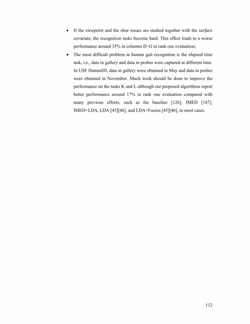
112
• If the viewpoint and the shoe issues are studied together with the surface
covariate, the recognition tasks become hard. This effect leads to a worse
performance around 35% in columns D–G in rank one evaluation;
• The most difficult problem in human gait recognition is the elapsed time
task, i.e., data in gallery and data in probes were captured at different time.
In USF HumanID, data in gallery were obtained in May and data in probes
were obtained in November. Much work should be done to improve the
performance on the tasks K and L although our proposed algorithms report
better performance around 17% in rank one evaluation compared with
many previous efforts, such as the baseline [126], IMED [167],
IMED+LDA, LDA [45][46], and LDA+Fusion [45][46], in most cases.
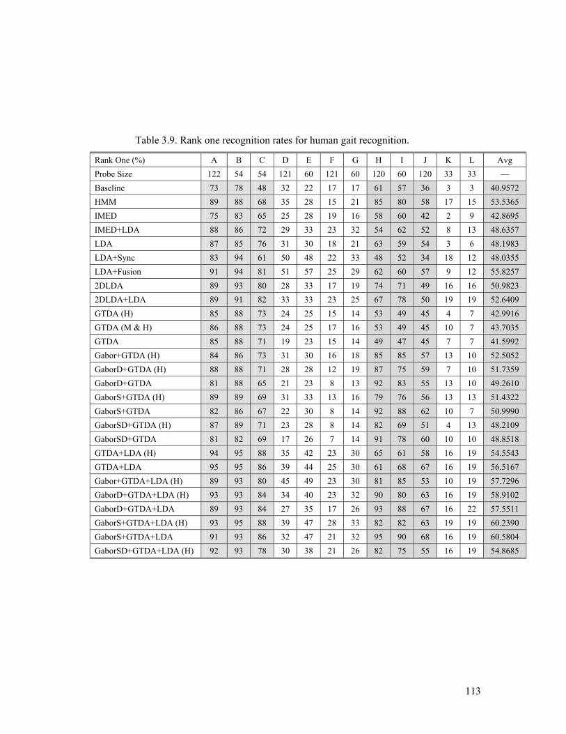
113
Table 3.9. Rank one recognition rates for human gait recognition.
Rank One (%) A B C D E F G H I J K L Avg Probe Size 122 54 54 121 60 121 60 120 60 120 33 33 –– Baseline 73 78 48 32 22 17 17 61 57 36 3 3 40.9572 HMM 89 88 68 35 28 15 21 85 80 58 17 15 53.5365 IMED 75 83 65 25 28 19 16 58 60 42 2 9 42.8695 IMED+LDA 88 86 72 29 33 23 32 54 62 52 8 13 48.6357 LDA 87 85 76 31 30 18 21 63 59 54 3 6 48.1983 LDA+Sync 83 94 61 50 48 22 33 48 52 34 18 12 48.0355 LDA+Fusion 91 94 81 51 57 25 29 62 60 57 9 12 55.8257 2DLDA 89 93 80 28 33 17 19 74 71 49 16 16 50.9823 2DLDA+LDA 89 91 82 33 33 23 25 67 78 50 19 19 52.6409 GTDA (H) 85 88 73 24 25 15 14 53 49 45 4 7 42.9916 GTDA (M & H) 86 88 73 24 25 17 16 53 49 45 10 7 43.7035 GTDA 85 88 71 19 23 15 14 49 47 45 7 7 41.5992 Gabor+GTDA (H) 84 86 73 31 30 16 18 85 85 57 13 10 52.5052 GaborD+GTDA (H) 88 88 71 28 28 12 19 87 75 59 7 10 51.7359 GaborD+GTDA 81 88 65 21 23 8 13 92 83 55 13 10 49.2610 GaborS+GTDA (H) 89 89 69 31 33 13 16 79 76 56 13 13 51.4322 GaborS+GTDA 82 86 67 22 30 8 14 92 88 62 10 7 50.9990 GaborSD+GTDA (H) 87 89 71 23 28 8 14 82 69 51 4 13 48.2109 GaborSD+GTDA 81 82 69 17 26 7 14 91 78 60 10 10 48.8518 GTDA+LDA (H) 94 95 88 35 42 23 30 65 61 58 16 19 54.5543 GTDA+LDA 95 95 86 39 44 25 30 61 68 67 16 19 56.5167 Gabor+GTDA+LDA (H) 89 93 80 45 49 23 30 81 85 53 10 19 57.7296 GaborD+GTDA+LDA (H) 93 93 84 34 40 23 32 90 80 63 16 19 58.9102 GaborD+GTDA+LDA 89 93 84 27 35 17 26 93 88 67 16 22 57.5511 GaborS+GTDA+LDA (H) 93 95 88 39 47 28 33 82 82 63 19 19 60.2390 GaborS+GTDA+LDA 91 93 86 32 47 21 32 95 90 68 16 19 60.5804 GaborSD+GTDA+LDA (H) 92 93 78 30 38 21 26 82 75 55 16 19 54.8685
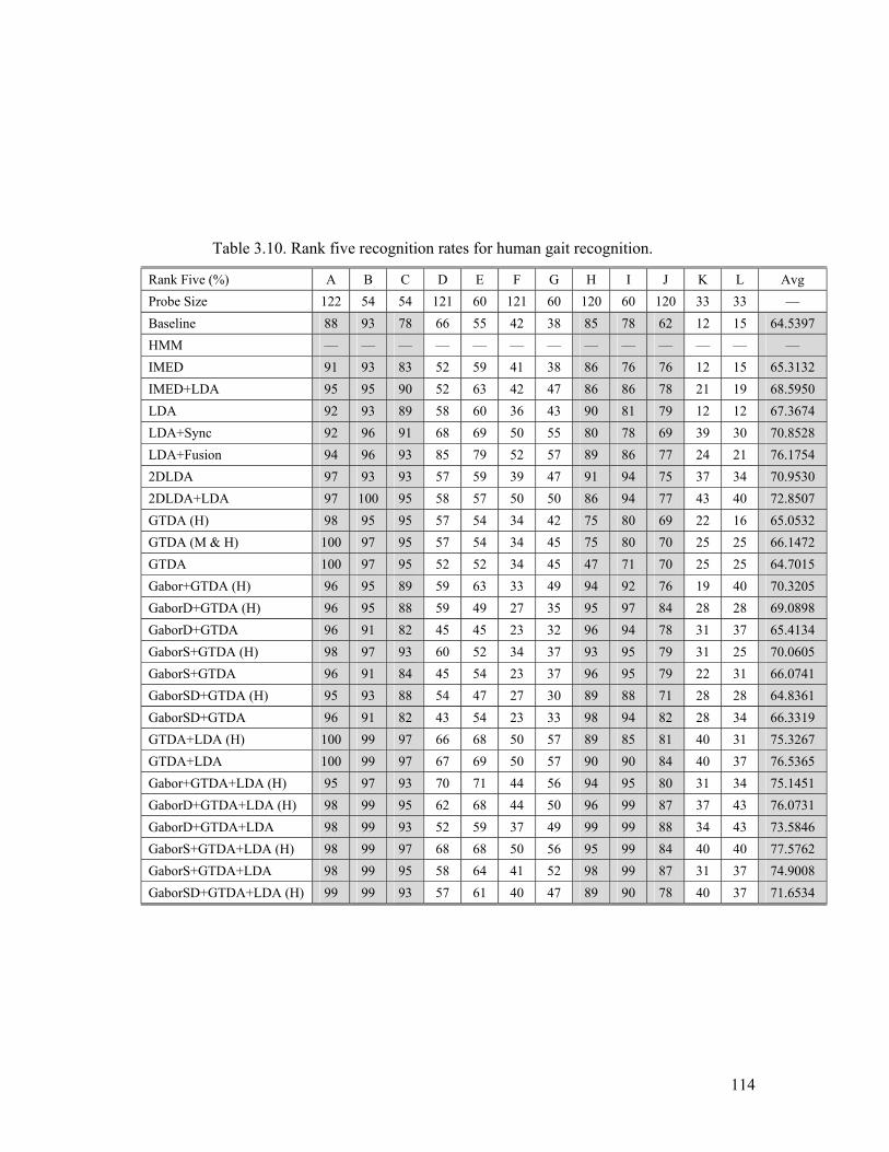
114
Table 3.10. Rank five recognition rates for human gait recognition.
Rank Five (%) A B C D E F G H I J K L Avg Probe Size 122 54 54 121 60 121 60 120 60 120 33 33 –– Baseline 88 93 78 66 55 42 38 85 78 62 12 15 64.5397 HMM –– –– –– –– –– –– –– –– –– –– –– –– –– IMED 91 93 83 52 59 41 38 86 76 76 12 15 65.3132 IMED+LDA 95 95 90 52 63 42 47 86 86 78 21 19 68.5950 LDA 92 93 89 58 60 36 43 90 81 79 12 12 67.3674 LDA+Sync 92 96 91 68 69 50 55 80 78 69 39 30 70.8528 LDA+Fusion 94 96 93 85 79 52 57 89 86 77 24 21 76.1754 2DLDA 97 93 93 57 59 39 47 91 94 75 37 34 70.9530 2DLDA+LDA 97 100 95 58 57 50 50 86 94 77 43 40 72.8507 GTDA (H) 98 95 95 57 54 34 42 75 80 69 22 16 65.0532 GTDA (M & H) 100 97 95 57 54 34 45 75 80 70 25 25 66.1472 GTDA 100 97 95 52 52 34 45 47 71 70 25 25 64.7015 Gabor+GTDA (H) 96 95 89 59 63 33 49 94 92 76 19 40 70.3205 GaborD+GTDA (H) 96 95 88 59 49 27 35 95 97 84 28 28 69.0898 GaborD+GTDA 96 91 82 45 45 23 32 96 94 78 31 37 65.4134 GaborS+GTDA (H) 98 97 93 60 52 34 37 93 95 79 31 25 70.0605 GaborS+GTDA 96 91 84 45 54 23 37 96 95 79 22 31 66.0741 GaborSD+GTDA (H) 95 93 88 54 47 27 30 89 88 71 28 28 64.8361 GaborSD+GTDA 96 91 82 43 54 23 33 98 94 82 28 34 66.3319 GTDA+LDA (H) 100 99 97 66 68 50 57 89 85 81 40 31 75.3267 GTDA+LDA 100 99 97 67 69 50 57 90 90 84 40 37 76.5365 Gabor+GTDA+LDA (H) 95 97 93 70 71 44 56 94 95 80 31 34 75.1451 GaborD+GTDA+LDA (H) 98 99 95 62 68 44 50 96 99 87 37 43 76.0731 GaborD+GTDA+LDA 98 99 93 52 59 37 49 99 99 88 34 43 73.5846 GaborS+GTDA+LDA (H) 98 99 97 68 68 50 56 95 99 84 40 40 77.5762 GaborS+GTDA+LDA 98 99 95 58 64 41 52 98 99 87 31 37 74.9008 GaborSD+GTDA+LDA (H) 99 99 93 57 61 40 47 89 90 78 40 37 71.6534
115
1 2 3 4 5 6 7 8 9 10 1182
84
86
88
90
92
94
96
98
Algorithm#
Ran
k 1
Rec
ogni
tion
Rat
e
Performance Comparison on ProbeA
1 2 3 4 5 6 7 8 9 10 1180
85
90
95
Algorithm#
Ran
k 1
Rec
ogni
tion
Rat
e
Performance Comparison on ProbeB
1 2 3 4 5 6 7 8 9 10 1165
70
75
80
85
90
Algorithm#
Ran
k 1
Rec
ogni
tion
Rat
e
Performance Comparison on ProbeC
1 2 3 4 5 6 7 8 9 10 11
30
35
40
45
50
Algorithm#R
ank
1 R
ecog
nitio
n R
ate
Performance Comparison on ProbeD
1 2 3 4 5 6 7 8 9 10 11
30
35
40
45
50
55
Algorithm#
Ran
k 1
Rec
ogni
tion
Rat
e
Performance Comparison on ProbeE
1 2 3 4 5 6 7 8 9 10 1114
16
18
20
22
24
26
28
Algorithm#
Ran
k 1
Rec
ogni
tion
Rat
ePerformance Comparison on ProbeF
1 2 3 4 5 6 7 8 9 10 11
20
22
24
26
28
30
32
34
Algorithm#
Ran
k 1
Rec
ogni
tion
Rat
e
Performance Comparison on ProbeG
1 2 3 4 5 6 7 8 9 10 11
55
60
65
70
75
80
85
90
Algorithm#
Ran
k 1
Rec
ogni
tion
Rat
e
Performance Comparison on ProbeH
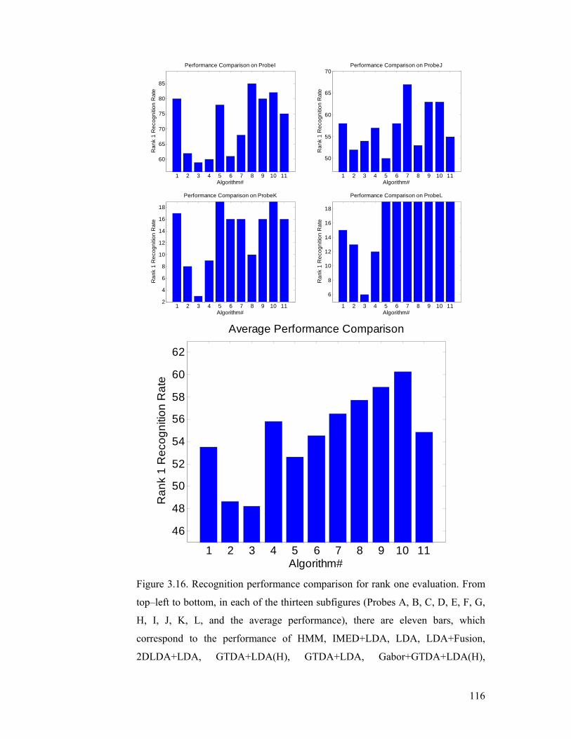
116
1 2 3 4 5 6 7 8 9 10 11
60
65
70
75
80
85
Algorithm#
Ran
k 1
Rec
ogni
tion
Rat
e
Performance Comparison on ProbeI
1 2 3 4 5 6 7 8 9 10 11
50
55
60
65
70
Algorithm#
Ran
k 1
Rec
ogni
tion
Rat
e
Performance Comparison on ProbeJ
1 2 3 4 5 6 7 8 9 10 112
4
6
8
10
12
14
16
18
Algorithm#
Ran
k 1
Rec
ogni
tion
Rat
e
Performance Comparison on ProbeK
1 2 3 4 5 6 7 8 9 10 11
6
8
10
12
14
16
18
Algorithm#R
ank
1 R
ecog
nitio
n R
ate
Performance Comparison on ProbeL
1 2 3 4 5 6 7 8 9 10 11
46
48
50
52
54
56
58
60
62
Algorithm#
Ran
k 1
Rec
ogni
tion
Rat
e
Average Performance Comparison
Figure 3.16. Recognition performance comparison for rank one evaluation. From
top–left to bottom, in each of the thirteen subfigures (Probes A, B, C, D, E, F, G,
H, I, J, K, L, and the average performance), there are eleven bars, which
correspond to the performance of HMM, IMED+LDA, LDA, LDA+Fusion,
2DLDA+LDA, GTDA+LDA(H), GTDA+LDA, Gabor+GTDA+LDA(H),
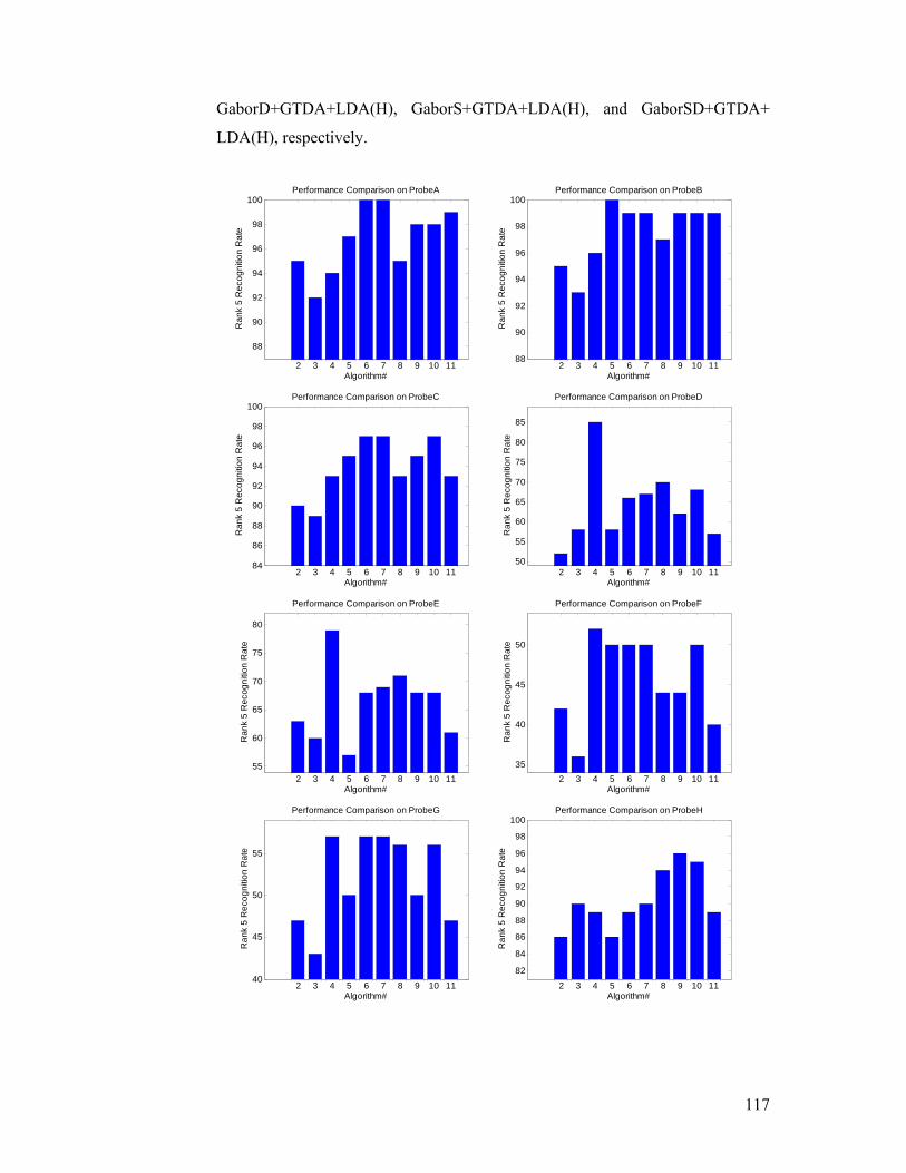
117
GaborD+GTDA+LDA(H), GaborS+GTDA+LDA(H), and GaborSD+GTDA+
LDA(H), respectively.
2 3 4 5 6 7 8 9 10 11
88
90
92
94
96
98
100
Algorithm#
Ran
k 5
Rec
ogni
tion
Rat
e
Performance Comparison on ProbeA
2 3 4 5 6 7 8 9 10 1188
90
92
94
96
98
100
Algorithm#
Ran
k 5
Rec
ogni
tion
Rat
e
Performance Comparison on ProbeB
2 3 4 5 6 7 8 9 10 1184
86
88
90
92
94
96
98
100
Algorithm#
Ran
k 5
Rec
ogni
tion
Rat
e
Performance Comparison on ProbeC
2 3 4 5 6 7 8 9 10 1150
55
60
65
70
75
80
85
Algorithm#
Ran
k 5
Rec
ogni
tion
Rat
e
Performance Comparison on ProbeD
2 3 4 5 6 7 8 9 10 1155
60
65
70
75
80
Algorithm#
Ran
k 5
Rec
ogni
tion
Rat
e
Performance Comparison on ProbeE
2 3 4 5 6 7 8 9 10 1135
40
45
50
Algorithm#
Ran
k 5
Rec
ogni
tion
Rat
e
Performance Comparison on ProbeF
2 3 4 5 6 7 8 9 10 1140
45
50
55
Algorithm#
Ran
k 5
Rec
ogni
tion
Rat
e
Performance Comparison on ProbeG
2 3 4 5 6 7 8 9 10 11
82
84
86
88
90
92
94
96
98
100
Algorithm#
Ran
k 5
Rec
ogni
tion
Rat
e
Performance Comparison on ProbeH
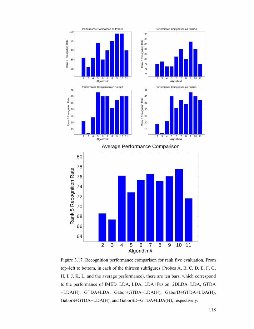
118
2 3 4 5 6 7 8 9 10 11
80
85
90
95
100
Algorithm#
Ran
k 5
Rec
ogni
tion
Rat
e
Performance Comparison on ProbeI
2 3 4 5 6 7 8 9 10 11
74
76
78
80
82
84
86
88
90
Algorithm#
Ran
k 5
Rec
ogni
tion
Rat
e
Performance Comparison on ProbeJ
2 3 4 5 6 7 8 9 10 11
15
20
25
30
35
40
45
Algorithm#
Ran
k 5
Rec
ogni
tion
Rat
e
Performance Comparison on ProbeK
2 3 4 5 6 7 8 9 10 11
15
20
25
30
35
40
45
Algorithm#R
ank
5 R
ecog
nitio
n R
ate
Performance Comparison on ProbeL
2 3 4 5 6 7 8 9 10 11
64
66
68
70
72
74
76
78
80
Algorithm#
Ran
k 5
Rec
ogni
tion
Rat
e
Average Performance Comparison
Figure 3.17. Recognition performance comparison for rank five evaluation. From
top–left to bottom, in each of the thirteen subfigures (Probes A, B, C, D, E, F, G,
H, I, J, K, L, and the average performance), there are ten bars, which correspond
to the performance of IMED+LDA, LDA, LDA+Fusion, 2DLDA+LDA, GTDA
+LDA(H), GTDA+LDA, Gabor+GTDA+LDA(H), GaborD+GTDA+LDA(H),
GaborS+GTDA+LDA(H), and GaborSD+GTDA+LDA(H), respectively.
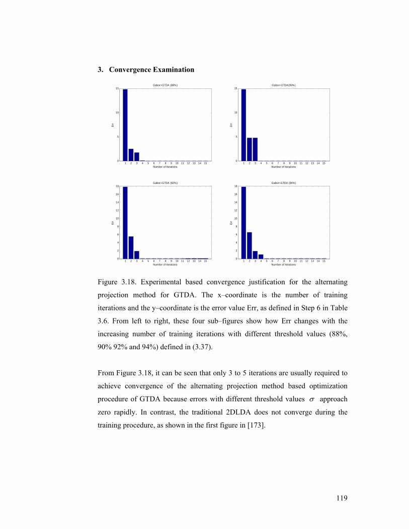
119
3. Convergence Examination
1 2 3 4 5 6 7 8 9 10 11 12 13 14 150
5
10
15
Number of Iterations
Err
Gabor+GTDA (88%)
1 2 3 4 5 6 7 8 9 10 11 12 13 14 150
5
10
15
Number of Iterations
Err
Gabor+GTDA(90%)
1 2 3 4 5 6 7 8 9 10 11 12 13 14 150
2
4
6
8
10
12
14
16
18
Number of Iterations
Err
Gabor+GTDA (92%)
1 2 3 4 5 6 7 8 9 10 11 12 13 14 150
2
4
6
8
10
12
14
16
18
Number of Iterations
Err
Gabor+GTDA (94%)
Figure 3.18. Experimental based convergence justification for the alternating
projection method for GTDA. The x–coordinate is the number of training
iterations and the y–coordinate is the error value Err, as defined in Step 6 in Table
3.6. From left to right, these four sub–figures show how Err changes with the
increasing number of training iterations with different threshold values (88%,
90% 92% and 94%) defined in (3.37).
From Figure 3.18, it can be seen that only 3 to 5 iterations are usually required to
achieve convergence of the alternating projection method based optimization
procedure of GTDA because errors with different threshold values σ approach
zero rapidly. In contrast, the traditional 2DLDA does not converge during the
training procedure, as shown in the first figure in [173].
120
Summary
Objects in computer vision research are naturally represented by general tensors.
The most popular examples are images and video shots, e.g., face images in face
recognition and video shots in video categorization. However, tensors have in the
past been reduced to the vector form, because available subspace selection
methods do not accept tensors as input. The vectorization removes the structure
information, which could reduce the number of parameters needed to model the
samples (images and video shots). To preserve the structure information, we
develop the general tensor discriminant analysis (GTDA) for discriminative
multilinear susbapce selection. This is an effective and efficient preprocessing
step for subsequent classification, e.g. by linear discriminant analysis (LDA).
Compared with existing multilinear subspace selection methods, e.g., the general
tensor analysis (GTA) and the two dimensional LDA (2DLDA), the advantages of
the proposed GTDA are: 1) the proposed alternating projection method to obtain a
solution of GTDA converges; 2) GTDA accepts general tensors as input; 3)
GTDA takes the discriminative information into account; and 4) GTDA reduces
the SSS problem of the subsequent classification, e.g., by LDA. We further
develop the manifold learning using tensor representations, which is an extension
of GTDA based on the graph embedding framework. With this new framework,
most of the popular manifold learning algorithms accept tensors as input. Finally,
we apply GTDA to human gait recognition and achieve top level performance.
121
4. Supervised Tensor Learning
In vector based learning15 [30][39], a projection vector Lw R∈r and a bias b R∈
are learnt to determine the class label of a sample Lx R∈r according to a linear
decision function ( ) sign Ty x w x b⎡ ⎤= +⎣ ⎦r r r . The wr and b are obtained based on
a learning model, e.g., minimax probability machine (MPM) [74][135], based on
N training samples associated with labels { },Li ix R y∈r , where iy is the class
label, { }1, 1iy ∈ + − , and 1 i N≤ ≤ . In this Chapter, we focus on the convex
optimization based learning, which accept vectors as input.
Supervised tensor learning (STL) [149][150] is developed to extend the vector
based learning algorithms to accept tensors as input. That is we learn a series of
projection vectors 1| kLMk kw R= ∈r and a bias b R∈ to determine the class label
{ }1, 1+ − of a sample 1 2 ML L LR × ×∈X L according to a multilinear decision function
( )1
signk
M
kk
y w b×=
⎡ ⎤= +⎢ ⎥
⎣ ⎦∏X X r . The 1|Mk kw =
r and b are obtained from a learning
model, e.g., tensor minimax probability machine (TMPM), based on N training
samples associated with labels { }1 2 ,ML L Li iR y× ×∈X L , where iy is the class label,
{ }1, 1iy ∈ + − , and 1 i N≤ ≤ .
This extension to tensor input is important, because many objects in computer
vision research are represented by general tensors in 1 2 ML L LR × ×L , as described in
Chapter 3. If we choose to use vector based learning algorithms, the vectorization
operation ( )vect ⋅ is applied to a general tensor X and form a vector
( )vect Lx R= ∈Xr , where 1 2 ML L L L= × ×L . The vectorization eliminates the
structure information of a sample in its original format. However, the information
is helpful to reduce the number of parameters in a learning model and result in
alleviating the overfitting problem. Usually, the testing error decreases with
respect to the increasing complexity of training samples. When the complexity of
training samples (partially represented by the number of training samples) is
15 We refer to the binary classification tasks.
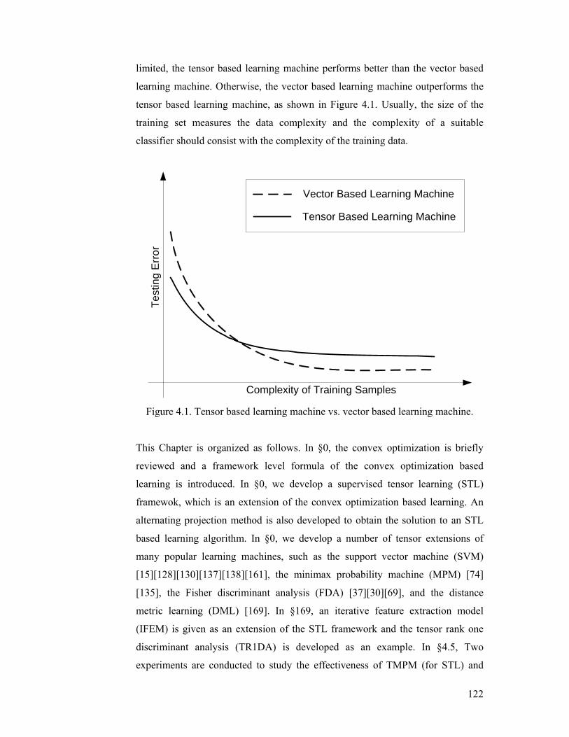
122
limited, the tensor based learning machine performs better than the vector based
learning machine. Otherwise, the vector based learning machine outperforms the
tensor based learning machine, as shown in Figure 4.1. Usually, the size of the
training set measures the data complexity and the complexity of a suitable
classifier should consist with the complexity of the training data.
Complexity of Training Samples
Test
ing
Err
or
Vector Based Learning Machine
Tensor Based Learning Machine
Figure 4.1. Tensor based learning machine vs. vector based learning machine.
This Chapter is organized as follows. In §0, the convex optimization is briefly
reviewed and a framework level formula of the convex optimization based
learning is introduced. In §0, we develop a supervised tensor learning (STL)
framewok, which is an extension of the convex optimization based learning. An
alternating projection method is also developed to obtain the solution to an STL
based learning algorithm. In §0, we develop a number of tensor extensions of
many popular learning machines, such as the support vector machine (SVM)
[15][128][130][137][138][161], the minimax probability machine (MPM) [74]
[135], the Fisher discriminant analysis (FDA) [37][30][69], and the distance
metric learning (DML) [169]. In §169, an iterative feature extraction model
(IFEM) is given as an extension of the STL framework and the tensor rank one
discriminant analysis (TR1DA) is developed as an example. In §4.5, Two
experiments are conducted to study the effectiveness of TMPM (for STL) and

123
TR1DA (for IFEM) empirically. The first experiment, for image classification,
demonstrates that TMPM reduces the overfitting problem in MPM. The second
experiment, for the elapsed time problem in human gait recognition, shows
TR1DA is more effective than PCA, LDA, and TR1A. Frinally, we summarize
this Chapter in §169.
124
Convex Optimization based Learning
Learning models are always formulated as optimization problems [170][178].
Therefore, mathematical programming [170][178] is the heart of machine learning
research [128]. In this Section, we first introduce the fundamentals of convex
optimization and then give a general formulation for convex optimization based
learning.
A mathematical programming problem [170][178][11] has the form or it can be
transformed to this form
( )( )( )
0min
0, 1s.t.
0, 1
w
i
i
f w
f w i mh w i p
⎡ ⎤⎢ ⎥⎢ ⎥≤ ≤ ≤⎢ ⎥= ≤ ≤⎣ ⎦
r
r
r
r, (4.1)
where 1 2[ , , , ]T nnw w w w R= ∈
rL is the optimization variable in (4.1); the function
0 : nf R R→ is the objective function; the functions : nif R R→ are inequality
constraint functions; and the functions : nih R R→ are equality constraint
functions. A vector *wr is a solution to the problem if 0f achieves its minimum
among all possible vectors, i.e., all vectors which satisfy the constraint equations
( 1|mi if = and 1|pi ih = ).
When the objective function ( )0f wr and the inequality constraint functions
( ) 1|mi if w =r satisfy
( ) ( ) ( )1 2 1 2
1 2
, and 1
,
i i i
n
f w w f w f wR
w w R
α β α βα β α β+
+ ≤ +
∈ + =
∈
r r r r
r (4.2)
(i.e., ( ) 0|mi if w =r are convex functions) and the equality constraint functions
( ) 1|pi ih w =r are affine (i.e., ( ) 0ih w =
r can be simplified as Ti ia w b=r r ), the
mathematical programming problem defined in (4.1) is named the convex
optimization problem. Therefore, a convex optimization problem [11] is defined
by
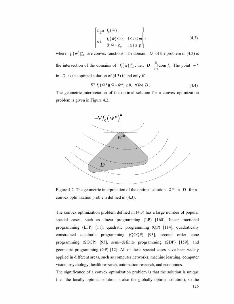
125
( )( )
0min
0, 1s.t.
, 1
w
iTi i
f w
f w i ma w b i p
⎡ ⎤⎢ ⎥⎢ ⎥≤ ≤ ≤⎢ ⎥= ≤ ≤⎣ ⎦
r
r
r
r r, (4.3)
where ( ) 0|mi if w =
r are convex functions. The domain D of the problem in (4.3) is
the intersection of the domains of ( ) 0|mi if w =r , i.e.,
0dom
m
ii
D f=
= I . The point *wr
in D is the optimal solution of (4.3) if and only if
( )( )0 * * 0, T f w w w w D∇ − ≥ ∀ ∈r r r r . (4.4)
The geometric interpretation of the optimal solution for a convex optimization
problem is given in Figure 4.2.
D
*wr
( )0 *f w−∇r
Figure 4.2. The geometric interpretation of the optimal solution *wr in D for a
convex optimization problem defined in (4.3).
The convex optimization problem defined in (4.3) has a large number of popular
special cases, such as linear programming (LP) [160], linear fractional
programming (LFP) [11], quadratic programming (QP) [114], quadratically
constrained quadratic programming (QCQP) [93], second order cone
programming (SOCP) [93], semi–definite programming (SDP) [159], and
geometric programming (GP) [12]. All of these special cases have been widely
applied in different areas, such as computer networks, machine learning, computer
vision, psychology, health research, automation research, and economics.
The significance of a convex optimization problem is that the solution is unique
(i.e., the locally optimal solution is also the globally optimal solution), so the
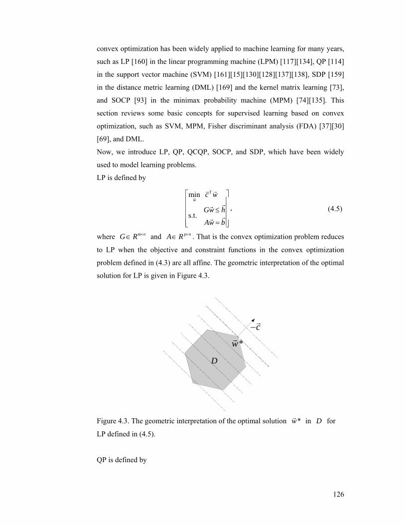
126
convex optimization has been widely applied to machine learning for many years,
such as LP [160] in the linear programming machine (LPM) [117][134], QP [114]
in the support vector machine (SVM) [161][15][130][128][137][138], SDP [159]
in the distance metric learning (DML) [169] and the kernel matrix learning [73],
and SOCP [93] in the minimax probability machine (MPM) [74][135]. This
section reviews some basic concepts for supervised learning based on convex
optimization, such as SVM, MPM, Fisher discriminant analysis (FDA) [37][30]
[69], and DML.
Now, we introduce LP, QP, QCQP, SOCP, and SDP, which have been widely
used to model learning problems.
LP is defined by
min
s.t.
T
wc w
Gw h
Aw b
⎡ ⎤⎢ ⎥⎢ ⎥≤⎢ ⎥
=⎢ ⎥⎣ ⎦
r
r r
rr
rr
, (4.5)
where m nG R ×∈ and p nA R ×∈ . That is the convex optimization problem reduces
to LP when the objective and constraint functions in the convex optimization
problem defined in (4.3) are all affine. The geometric interpretation of the optimal
solution for LP is given in Figure 4.3.
D
*wrc−r
Figure 4.3. The geometric interpretation of the optimal solution *wr in D for
LP defined in (4.5).
QP is defined by
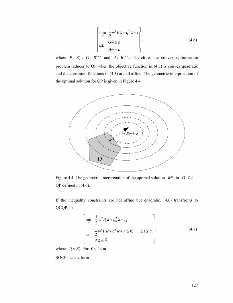
127
1min 2
s.t.
T T
ww Pw q w r
Gw h
Aw b
⎡ ⎤+ +⎢ ⎥⎢ ⎥
≤⎢ ⎥⎢ ⎥
=⎣ ⎦
r
r r r r
rr
rr
, (4.6)
where nP S+∈ , m nG R ×∈ and p nA R ×∈ . Therefore, the convex optimization
problem reduces to QP when the objective function in (4.3) is convex quadratic
and the constraint functions in (4.3) are all affine. The geometric interpretation of
the optimal solution for QP is given in Figure 4.4.
D
*wr( )Pw q− +
r r
Figure 4.4. The geometric interpretation of the optimal solution *wr in D for
QP defined in (4.6).
If the inequality constraints are not affine but quadratic, (4.6) transfroms to
QCQP, i.e.,
0 0 01min 21 0, 12s.t.
T T
w
T Ti i i
w P w q w r
w Pw q w r i m
Aw b
⎡ ⎤+ +⎢ ⎥⎢ ⎥⎢ ⎥+ + ≤ ≤ ≤⎢ ⎥⎢ ⎥
=⎣ ⎦
r
r r r r
r r r r
rr
, (4.7)
where niP S+∈ for 0 i m≤ ≤ .
SOCP has the form
128
min
, 1s.t.
T
wT
i i i iFro
f w
A w b c w d i mFw g
⎡ ⎤⎢ ⎥⎢ ⎥+ ≤ + ≤ ≤⎢ ⎥
=⎣ ⎦
r
r r
r r r
r r, (4.8)
where in niA R ×∈ , p nF R ×∈ , n
ic R∈r , pg R∈
r , inib R∈ , and id R∈ . The
constraint with the form TAw b c w d+ ≤ +r r r is called the second order cone
constraint. When 0ic =r for all 1 i m≤ ≤ , SOCP transforms to QCQP.
Recently, SDP has become an increasingly important technique in machine
learning and many SDP based learning machines have been developed. SDP
minimizes a linear function subject to a matrix semidefinite constraint
( ) 01
min c
s.t. 0
T
w
n
i ii
w
F w F w F=
⎡ ⎤⎢ ⎥⎢ ⎥
+ ≥⎢ ⎥⎣ ⎦
∑
r
r r
r , (4.9)
where miF S∈ for all 0 i n≤ ≤ and nc R∈
r .
Here, we provide a general formula for convex optimization based learning as
( )( )
, ,min , ,
s.t. , 1w b
Ti i i i
f w b
y c w x b i Nξ
ξ
ξ
⎡ ⎤⎢ ⎥⎢ ⎥+ ≥ ≤ ≤⎣ ⎦
rr
rr
r r , (4.10)
where 1: L Nf R R+ + → is a criterion (convex function) for classification;
:ic R R→ for all 1 i N≤ ≤ are convex constraint functions; Lix R∈r
(1 i N≤ ≤ ) are training samples and their class labels are given by { }1, 1iy ∈ + − ;
[ ]1 2, , , T NN Rξ ξ ξ ξ= ∈
rL are slack variables; and Lw R∈
r and b R∈ determine
a classification hyperplane, i.e., 0Tw x b+ =r r . By defining different classification
criteria f and convex constraint functions 1|Ni ic = , we can obtain a large number
of learning machines, such as SVM, MPM, FDA, and DML. We detail this in the
next Section.
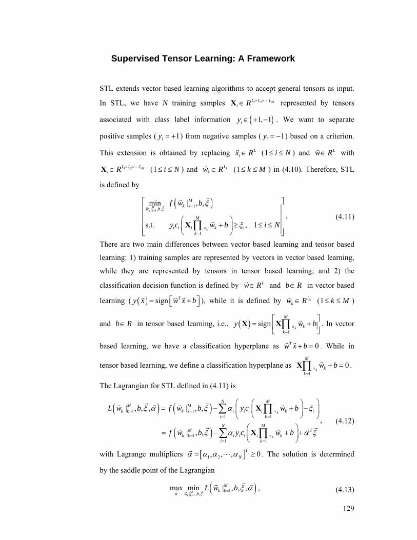
129
Supervised Tensor Learning: A Framework
STL extends vector based learning algorithms to accept general tensors as input.
In STL, we have N training samples 1 2 ML L Li R × ×∈X L represented by tensors
associated with class label information { }1, 1iy ∈ + − . We want to separate
positive samples ( 1iy = + ) from negative samples ( 1iy = − ) based on a criterion.
This extension is obtained by replacing Lix R∈r (1 i N≤ ≤ ) and Lw R∈
r with
1 2 ML L Li R × ×∈X L (1 i N≤ ≤ ) and kL
kw R∈r (1 k M≤ ≤ ) in (4.10). Therefore, STL
is defined by
( )1
1| , ,
1
min | , ,
s.t. , 1
Mk k
k
Mk k
w b
M
i i i k ik
f w b
y c w b i N
ξξ
ξ
==
×=
⎡ ⎤⎢ ⎥⎢ ⎥⎛ ⎞⎢ ⎥+ ≥ ≤ ≤⎜ ⎟⎢ ⎥⎝ ⎠⎣ ⎦
∏X
rr
rr
r. (4.11)
There are two main differences between vector based learning and tensor based
learning: 1) training samples are represented by vectors in vector based learning,
while they are represented by tensors in tensor based learning; and 2) the
classification decision function is defined by Lw R∈r and b R∈ in vector based
learning ( ( ) sign Ty x w x b⎡ ⎤= +⎣ ⎦r r r ), while it is defined by kL
kw R∈r (1 k M≤ ≤ )
and b R∈ in tensor based learning, i.e., ( )1
signk
M
kk
y w b×=
⎡ ⎤= +⎢ ⎥
⎣ ⎦∏X X r . In vector
based learning, we have a classification hyperplane as 0Tw x b+ =r r . While in
tensor based learning, we define a classification hyperplane as 1
0k
M
kk
w b×=
+ =∏X r .
The Lagrangian for STL defined in (4.11) is
( ) ( )
( )
1 11 1
11 1
| , , , | , ,
| , ,
k
k
MNM M
k k k k i i i i k ii k
MNM T
k k i i i i ki k
L w b f w b y c w b
f w b y c w b
ξ α ξ α ξ
ξ α α ξ
= = ×= =
= ×= =
⎛ ⎞⎛ ⎞= − + −⎜ ⎟⎜ ⎟
⎝ ⎠⎝ ⎠⎛ ⎞
= − + +⎜ ⎟⎝ ⎠
∑ ∏
∑ ∏
X
X
r rrr r r
r rrr r, (4.12)
with Lagrange multipliers [ ]1 2, , , 0TNα α α α= ≥
rL . The solution is determined
by the saddle point of the Lagrangian
( )1
1| , ,
max min | , , ,M
k k
Mk k
w bL w b
α ξξ α
==rr r
r rr , (4.13)
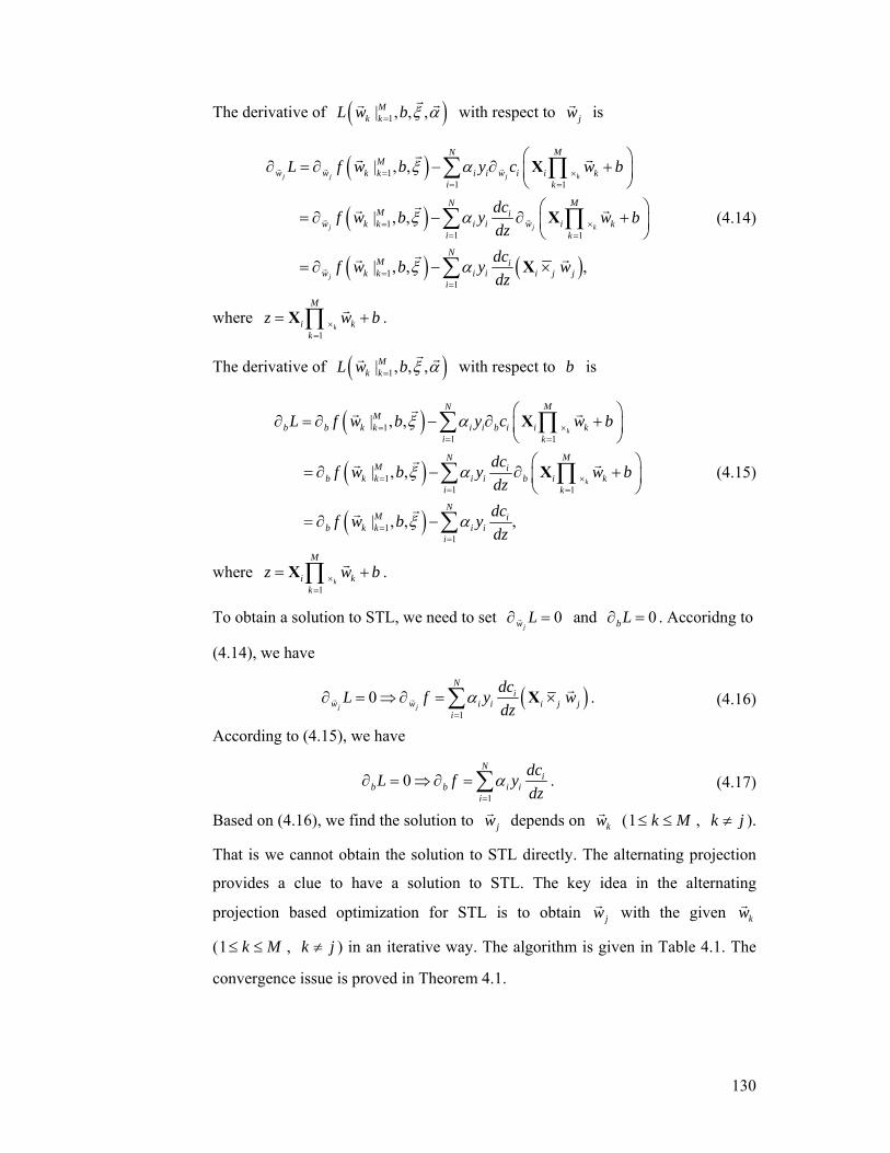
130
The derivative of ( )1| , , ,Mk kL w b ξ α=
r rr with respect to jwr is
( )
( )
( ) ( )
11 1
11 1
11
| , ,
| , ,
| , , ,
j j j k
j j k
j
MNM
w w k k i i w i i ki k
MNM i
w k k i i w i ki k
NM i
w k k i i i j ji
L f w b y c w b
dcf w b y w bdzdcf w b y wdz
ξ α
ξ α
ξ α
= ×= =
= ×= =
==
⎛ ⎞∂ = ∂ − ∂ +⎜ ⎟
⎝ ⎠⎛ ⎞
= ∂ − ∂ +⎜ ⎟⎝ ⎠
= ∂ − ×
∑ ∏
∑ ∏
∑
X
X
X
r r r
r r
r
rr r
rr r
rr r
(4.14)
where 1
k
M
i kk
z w b×=
= +∏X r .
The derivative of ( )1| , , ,Mk kL w b ξ α=
r rr with respect to b is
( )
( )
( )
11 1
11 1
11
| , ,
| , ,
| , , ,
k
k
MNM
b b k k i i b i i ki k
MNM i
b k k i i b i ki k
NM i
b k k i ii
L f w b y c w b
dcf w b y w bdzdcf w b ydz
ξ α
ξ α
ξ α
= ×= =
= ×= =
==
⎛ ⎞∂ = ∂ − ∂ +⎜ ⎟
⎝ ⎠⎛ ⎞
= ∂ − ∂ +⎜ ⎟⎝ ⎠
= ∂ −
∑ ∏
∑ ∏
∑
X
X
rr r
rr r
rr
(4.15)
where 1
k
M
i kk
z w b×=
= +∏X r .
To obtain a solution to STL, we need to set 0jw L∂ =r and 0bL∂ = . Accoridng to
(4.14), we have
( )1
0j j
Ni
w w i i i j ji
dcL f y wdz
α=
∂ = ⇒ ∂ = ×∑ Xr rr . (4.16)
According to (4.15), we have
1
0N
ib b i i
i
dcL f ydz
α=
∂ = ⇒ ∂ =∑ . (4.17)
Based on (4.16), we find the solution to jwr depends on kwr (1 k M≤ ≤ , k j≠ ).
That is we cannot obtain the solution to STL directly. The alternating projection
provides a clue to have a solution to STL. The key idea in the alternating
projection based optimization for STL is to obtain jwr with the given kwr
(1 k M≤ ≤ , k j≠ ) in an iterative way. The algorithm is given in Table 4.1. The
convergence issue is proved in Theorem 4.1.
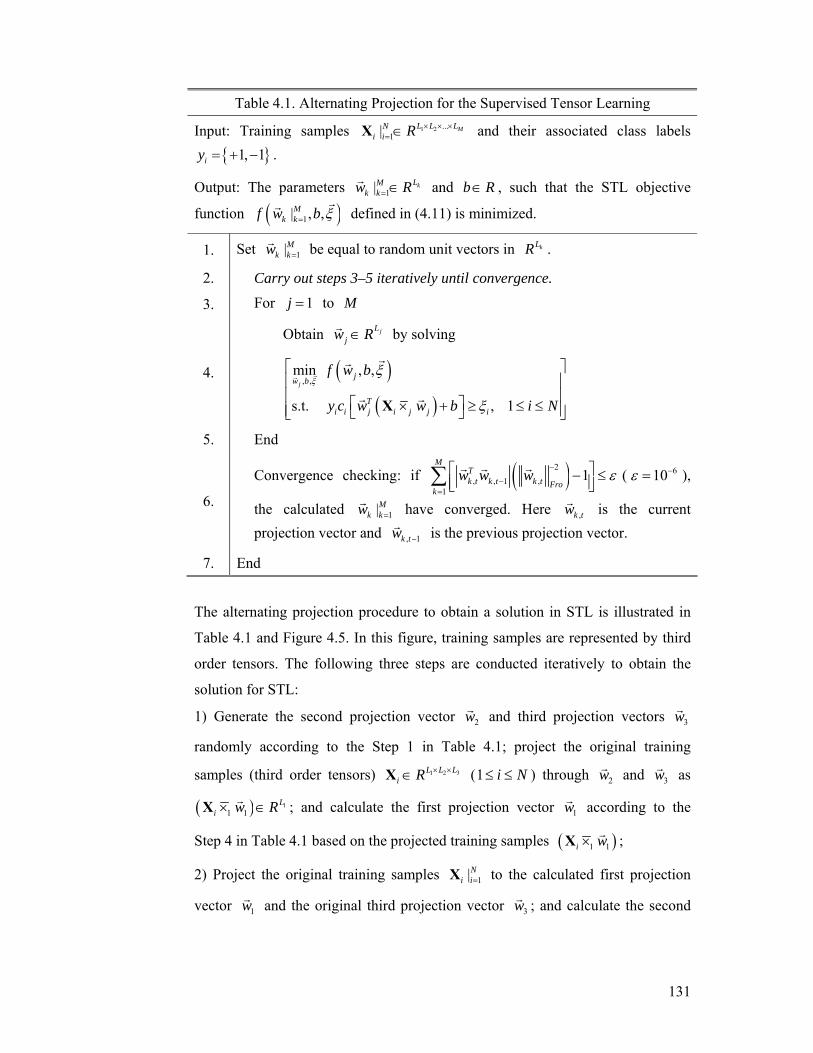
131
Table 4.1. Alternating Projection for the Supervised Tensor Learning
Input: Training samples 1 2 ...1| ML L LN
i i R × × ×= ∈X and their associated class labels
{ }1, 1iy = + − .
Output: The parameters 1| kLMk kw R= ∈r and b R∈ , such that the STL objective
function ( )1| , ,Mk kf w b ξ=
rr defined in (4.11) is minimized.
1. Set 1|Mk kw =r be equal to random unit vectors in kLR .
2. Carry out steps 3–5 iteratively until convergence.
3. For 1j = to M
4.
Obtain jLjw R∈r by solving
( )( )
, ,min , ,
s.t. , 1j
jw b
Ti i j i j j i
f w b
y c w w b i N
ξξ
ξ
⎡ ⎤⎢ ⎥⎢ ⎥⎡ ⎤× + ≥ ≤ ≤⎢ ⎥⎣ ⎦⎣ ⎦X
rr
rr
r r
5. End
6.
Convergence checking: if ( )2
, , 1 ,1
1M
Tk t k t k t Fro
k
w w w ε−
−=
⎡ ⎤− ≤⎢ ⎥⎣ ⎦∑ r r r ( 610ε −= ),
the calculated 1|Mk kw =r have converged. Here ,k twr is the current
projection vector and , 1k tw −r is the previous projection vector.
7. End
The alternating projection procedure to obtain a solution in STL is illustrated in
Table 4.1 and Figure 4.5. In this figure, training samples are represented by third
order tensors. The following three steps are conducted iteratively to obtain the
solution for STL:
1) Generate the second projection vector 2wr and third projection vectors 3wr
randomly according to the Step 1 in Table 4.1; project the original training
samples (third order tensors) 1 2 3L L Li R × ×∈X (1 i N≤ ≤ ) through 2wr and 3wr as
( ) 11 1
Li w R× ∈X r ; and calculate the first projection vector 1wr according to the
Step 4 in Table 4.1 based on the projected training samples ( )1 1i w×X r ;
2) Project the original training samples 1|Ni i=X to the calculated first projection
vector 1wr and the original third projection vector 3wr ; and calculate the second

132
projection vector 2wr according to the Step 4 in Table 4.1 based on the projected
training samples ( )2 2i w×X r ;
3) Project the original training samples 1|Ni i=X by the previous 1wr and 2wr ; and
calculate 3wr through the Step 4 in Table 4.1 based on the projected training
samples ( )3 3i w×X r .
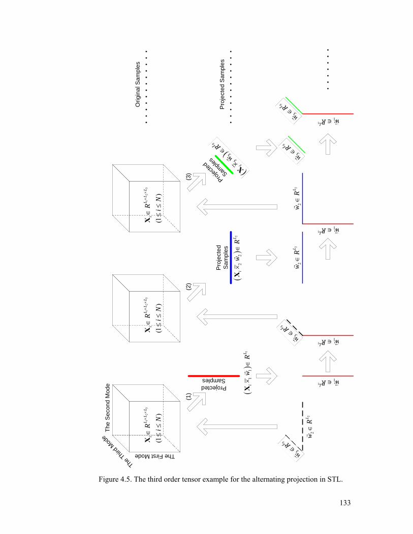
133
Figure 4.5. The third order tensor example for the alternating projection in STL.
()
11
1L
iw
R×
∈X
r
22
Lw
R∈
r
(1)
()
22
2L
iw
R×
∈X
r
22
Lw
R∈
r
12
3
(1)
LL
Li
R iN×
×∈ ≤≤
X
The First Mode
The
Sec
ond
Mod
e
The Thir
d Mod
e
12
3
(1)
LL
Li
R iN×
×∈ ≤≤
X
(2)
Projected Samples
12
3
(1)
LL
Li
R iN×
×∈ ≤≤
X
Pro
ject
ed
Sam
ples
22
Lw
R∈
r
(3)
Projec
ted
Sample
s
Orig
inal
Sam
ples
Pro
ject
ed S
ampl
es
134
Theorem 4.1 The alternating projection based optimization procedure for STL
converges.
Proof.
The alternating projection method never increases the function value
( )1| , ,Mk kf w b ξ=
rr of STL between two successive iterations, because it can be
interpreted as a type of a monotonic algorithm. We can define a continuous
function
1 2 1:
MN N
M kkf u u u R R u R R R
=× × × × × = × × × →L ,
where d dw u∈r and du is the set, which includes all possible dwr . The bias
b R∈ and the slack variables NRξ ∈r
.
With the definition, f has M different mappings:
( ) ( )( )
1, ,
11 1, ,
, , arg min | , ,
arg min , , ; | , | ,d d
d d
Md d d d du u b
d Md l l l l du u b
g w b f w b
f w b w w
ξ
ξ
ξ ξ
ξ
∗ ∗ ∗=∈
−= = +∈
=
rr
rr
r rr r
rr r r
The mapping can be calculated with the given 11|dl lw −=
r in the tth iteration and
1|Ml l dw = +r in the ( 1t − )th iteration of the for–loop in Step 4 in Table 4.1.
Given an initial d dw u∈r (1 d M≤ ≤ ), the alternating projection generates a
sequence of items { }, , ,, , ;1d t d t d tw b d Mξ∗ ∗ ∗ ≤ ≤rr via
( ) ( )1, , , , 1 , 1 1, ,, , arg min , , ; | , |
d d
d Md t d t d t d l t l l t l du u b
g w b f w b w wξ
ξ ξ∗ ∗ ∗ −= − = +∈
= rr
r rr r r r ,
with each { }1,2,d M∈ L . The sequence has the following relationship:
1,1 1,1 1,1 2,1 2,1 2,1 ,1 ,1 ,1 1,2 1,2 1,2
1, 1, 1, 2, 2, 2, 1, 1, 1, 2, 2, 2,
( , , ) ( , , ) ( , , ) ( , , )
( , , ) ( , , ) ( , , ) ( , , )
M M M
t t t t t t T T T T T T
a f w b f w b f w b f w b
f w b f w b f w b f w b
ξ ξ ξ ξ
ξ ξ ξ ξ
∗ ∗ ∗ ∗ ∗ ∗ ∗ ∗ ∗ ∗ ∗ ∗
∗ ∗ ∗ ∗ ∗ ∗ ∗ ∗ ∗ ∗ ∗ ∗
= ≥ ≥ ≥ ≥ ≥
≥ ≥ ≥ ≥ ≥ ≥
r r r rr r r rL
r r r rr r r rL L
, , , ( , , ) .M T M T M Tf w b bξ∗ ∗ ∗≥ =rr
L
where T →+∞ . Here both a and b are limited values in the R space.
The alternating projection in STL can be illustrated by a composition of M sub–
algorithms, defined as
( ) ( )1
11 1
: | , , Map , ,l l
d MM
d d d l d ll l d
w b w w b wξ ξ−
= × ×= = +
Ω ×∏ ∏r rr r r ra .

135
It follows that 1 2 1
M
M dd=Ω Ω Ω Ω = Ωo oLo o is a closed algorithm whenever all
du are compact. All sub–algorithms ( ), ,d d dg w b ξ∗ ∗ ∗rr decrease the value of f , so
it should be clear that Ω is monotonic with respect to f .
Consequently, we can say that the alternating projection method to optimize STL
defined in (4.11) converges. ■
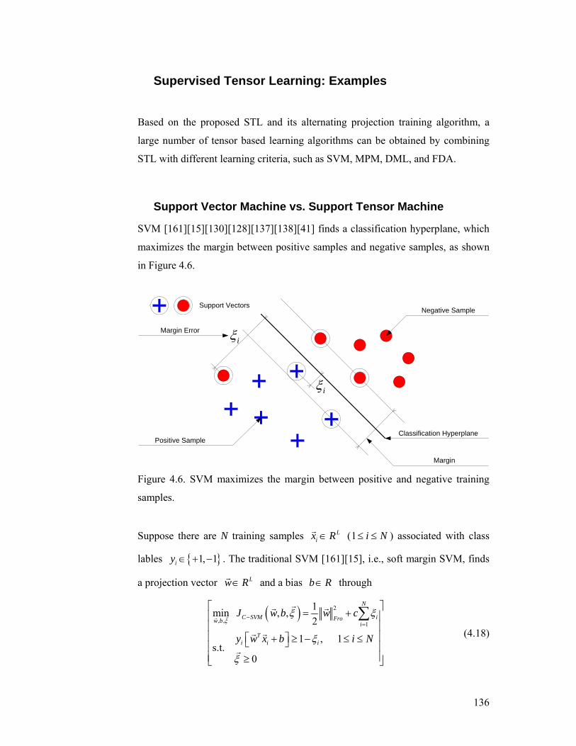
136
Supervised Tensor Learning: Examples
Based on the proposed STL and its alternating projection training algorithm, a
large number of tensor based learning algorithms can be obtained by combining
STL with different learning criteria, such as SVM, MPM, DML, and FDA.
Support Vector Machine vs. Support Tensor Machine
SVM [161][15][130][128][137][138][41] finds a classification hyperplane, which
maximizes the margin between positive samples and negative samples, as shown
in Figure 4.6.
Support Vectors
iξ
iξ
Positive Sample
Negative Sample
Classification Hyperplane
Margin
Margin Error
Figure 4.6. SVM maximizes the margin between positive and negative training
samples.
Suppose there are N training samples Lix R∈r (1 i N≤ ≤ ) associated with class
lables { }1, 1iy ∈ + − . The traditional SVM [161][15], i.e., soft margin SVM, finds
a projection vector Lw R∈r and a bias b R∈ through
( ) 2
, , 1
1min , ,2
1 , 1s.t.
0
N
C SVM iFrow b i
Ti i i
J w b w c
y w x b i N
ξξ ξ
ξ
ξ
−=
⎡ ⎤= +⎢ ⎥⎢ ⎥⎢ ⎥⎡ ⎤+ ≥ − ≤ ≤⎣ ⎦⎢ ⎥⎢ ⎥≥⎣ ⎦
∑rr
rr r
r r
r
(4.18)
137
where [ ]1 2, , , T NN Rξ ξ ξ ξ= ∈
rL is the vector of all slack variables to deal with
the linearly non–separable problem. The iξ ( 1 i N≤ ≤ ) is also called the
marginal error for the ith training sample, as shown in Figure 4.6. The margin is
2Fro
wr . When the classification problem is linearly separable, we can set 0ξ =r
.
The decision function for classification is ( ) sign Ty x w x b⎡ ⎤= +⎣ ⎦r r r .
The Lagrangian of (4.18) is
( ) ( )2
1 1 1
1 1 1
1, , , , 121 2
N N NT
i i i i i i iFroi i i
N N NT T T T T
i i i i ii i i
L w b w c y w x b
w w c y w x b y
ξ α κ ξ α ξ κ ξ
ξ α α α α ξ κ ξ
= = =
= = =
⎡ ⎤= + − + − + −⎣ ⎦
= + − − + − −
∑ ∑ ∑
∑ ∑ ∑
r r rr r r r
r rr r rr r r r r (4.19)
with Lagrangian multipliers 0iα ≥ , 0iκ ≥ for 1 i N≤ ≤ . The solution is
determined by the saddle point of the Lagrangian
( ), , ,
max min , , , ,w b
L w bα κ ξ
ξ α κrr r r
r r rr . (4.20)
This can be achieved by
10
0 00 0.
N
w i i ii
Tb
L w y x
L yL cξ
α
αα κ
=
∂ = ⇒ =
∂ = ⇒ =∂ = ⇒ − − =
∑r
r
r r
r r
r r (4.21)
Based on (4.21), we can have the dual problem of (4.18),
( )1 1 1
1max 2
0 s.t.
0
N N NT
D i j i j i j ii j i
T
J y y x x
yc
αα α α α
αα
= = =
⎡ ⎤= − +⎢ ⎥
⎢ ⎥⎢ ⎥=⎢ ⎥
≤ ≤⎢ ⎥⎣ ⎦
∑∑ ∑r
r r r
r r
r
. (4.22)
Set 1 ,
Ti j i j i j N
P y y x x≤ ≤
⎡ ⎤= ⎣ ⎦r r , 11Nq ×=
rr , A y=r , 0b =
r, [ ], T
N N N NG I I× ×= − , and
1 11 ,0TT T
N Nh c × ×⎡ ⎤= ⎣ ⎦r r r
in (4.6), we can see that the dual problem of (4.18) in SVM is a
QP.
In the soft margin SVM defined in (4.18), the constant c determines the tradeoff
between 1) maximizing the margin between positive and negative samples and 2)
minimizing the training error. The constant c is not intuitive. Therefore,
Bcholkopf et al. [130][128] developed the nu–SVM by replacing the unintuitive
parameter c with an intuitive parameter ν as
138
( ) 2
, , , 1
1 1min , , ,2
, 1
s.t. 0, 0
N
SVM iFrow b i
Ti i i
J w b wN
y w x b i N
νξ ρξ ρ ξ νρ
ρ ξ
ξρ
−=
⎡ ⎤= + −⎢ ⎥⎢ ⎥⎢ ⎥⎡ ⎤+ ≥ − ≤ ≤⎣ ⎦⎢ ⎥⎢ ⎥≥⎢ ⎥
≥⎣ ⎦
∑rr
rr r
r r
r. (4.23)
The significance of ν in nu–SVM defined in (4.23) is that it controls the number
of support vectors and the marginal errors.
Suykens and Vandewalle [137][138] simplified the soft margin SVM as the least
squares SVM,
( ) 2
, ,
1min , ,2 2
s.t. 1 , 1
TLS SVM Frow b
Ti i i
J w b w
y w x b i N
ε
γε ε ε
ε
−⎡ ⎤= +⎢ ⎥⎢ ⎥
⎡ ⎤+ = − ≤ ≤⎢ ⎥⎣ ⎦⎣ ⎦
rr
r r rr r
r r. (4.24)
Here the penalty 0γ > . There are two differences between the soft margin SVM
defined in (4.18) and the least squares SVM defined in (4.24): 1) inequality
constraints are replaced by equalities; and 2) the loss 1
Niiξ
=∑ ( 0iξ ≥ ) is replaced
by square loss. These two modifications make the solution of the least square
SVM be more easily obtained compared with soft margin SVM.
According to statistical learning theory, a learning machine performs well when
the number of training samples is larger than the complexity of the model.
Moreover, the model’s complexity and the number of parameters to describe the
model are always in direct proportion. In computer vision research, objects are
usually represented by general tensors as described in Chapter 3 and the number
of training samples is limited. Therefore, it is reasonable to have the tensor
extension of SVM i.e., the support tensor machine (STM), which uses fewer
parameters than SVM. Based on (4.18) and STL defined in (4.11), it is not
difficult to obtain the tensor extension of the soft margin SVM, i.e., the soft
margin STM.
Suppose we have training samples 1 2 ML L Li R × ×∈X L ( 1 i N≤ ≤ ) and their
corresponding class labels { }1, 1iy ∈ + − . The decision function is defined by
( )1
signk
M
kk
y w b×=
⎡ ⎤= +⎢ ⎥
⎣ ⎦∏X X r , where the projection vectors kL
kw R∈r (1 k M≤ ≤ )
and the bias b in soft margin STM are obtained from
139
( )1
2
1| , , 11
1
1min | , ,2
1 , 1 s.t.
0
Mk k
k
M NM
C STM k k k iw b ik Fro
M
i i k ik
J w b w c
y w b i N
ξξ ξ
ξ
ξ
=− = ⊗
==
×=
⎡ ⎤= +⎢ ⎥
⎢ ⎥⎢ ⎥⎡ ⎤⎢ ⎥+ ≥ − ≤ ≤⎢ ⎥⎢ ⎥⎣ ⎦⎢ ⎥
≥⎢ ⎥⎣ ⎦
∑∏
∏X
rr
rr r
r
r
. (4.25)
Here, [ ]1 2, , , T NN Rξ ξ ξ ξ= ∈
rL is the vector of all slack variables to deal with the
linearly non–separable problem.
The Lagrangian for this problem is
( )2
111
1 11
11 1
1| , , , ,2
1
1 2
k
k
M NM
k k k iik Fro
MN N
i i i k i i ii ik
M NTk k i i i i k
ik k
L w b w c
y w b
w w c y w
ξ α κ ξ
α ξ κ ξ
ξ α
= ⊗==
×= ==
×== =
= +
⎛ ⎞⎡ ⎤− + − + −⎜ ⎟⎢ ⎥
⎣ ⎦⎝ ⎠
= + −
∑∏
∑ ∑∏
∑∏
X
X
r r rr r
r
r r r
1
1
MN
i
NT T T
ii
b yα α α ξ κ ξ
=
=
⎛ ⎞⎜ ⎟⎝ ⎠
− + − −
∑ ∏
∑r rr r rr
(4.26)
with Lagrangian multipliers 0iα ≥ , 0iκ ≥ for 1 i N≤ ≤ . The solution is
determined by the saddle point of the Lagrangian
( )1
1, | , ,max min | , , , ,
Mk k
Mk k
w bL w b
α κ ξξ α κ
==rr r r
r r rr . (4.27)
This can be achieved by
( )1
1
10
0 00 0
j
N
w j i i i j jk jT ik k
k
Tb
L w y ww w
L yL cξ
α
αα κ
≠=
=
∂ = ⇒ = ×
∂ = ⇒ =∂ = ⇒ − − =
∑∏
Xr
r
r r
r r
r r
r r.
(4.28)
The first equation in (4.28) shows that the solution of jwr depends on kwr
(1 k M≤ ≤ , k j≠ ). That is we cannot obtain the solution for the soft margin
STM directly. This point has been pointed out in the STL framework developed in
§4.2. Therefore, we use the proposed alternating projection method in STL to
obtain the solution of the soft margin STM. To have the alternating projection
method for the soft margin STM, we need to replace the Step 4 in Table 4.1 by the
following optimization problem,
140
( )( )
2
, , 1min , ,
2
1 , 1s.t.
0
j
N
C STM j j iFrow b i
Ti j i j j i
J w b w c
y w w b i N
ξ
ηξ ξ
ξ
ξ
−=
⎡ ⎤= +⎢ ⎥⎢ ⎥⎢ ⎥⎡ ⎤× + ≥ − ≤ ≤⎣ ⎦⎢ ⎥⎢ ⎥≥⎣ ⎦
∑X
rr
rr r
r r
r
, (4.29)
where 2
1
k jk Frok M
wη ≠
≤ ≤=∏ r .
The problem defined in (4.29) is the standard soft margin SVM defined in (4.18).
Based on nu–SVM defined in (4.23) and STL defined in (4.11), we can also have
the tensor extension of the nu–SVM, i.e., nu–STM,
( )1
2
1| , , , 11
1
1 1min | , , ,2
, 1
s.t. 0, 0
Mk k
k
M NM
STM k k k iw b ik Fro
M
i i k ik
J w b wN
y w b i N
νξ ρ
ξ ρ ξ νρ
ρ ξ
ξρ
=− = ⊗
==
×=
= + −
⎡ ⎤+ ≥ − ≤ ≤⎢ ⎥
⎣ ⎦≥≥
∑∏
∏X
rr
rr r
r
r
⎡ ⎤⎢ ⎥⎢ ⎥⎢ ⎥⎢ ⎥⎢ ⎥⎢ ⎥⎢ ⎥⎢ ⎥⎣ ⎦
. (4.30)
Here, 0ν ≥ is a constant. The Lagrangian for this problem is
( )2
111
1 1
1
1 1| , , , , , ,2
1 1 2
k
M NM
k k k iik Fro
MNT
i i i k ii k
MTk k
k
L w b wN
y w b
w w
ξ ρ α κ τ ξ νρ τρ
α ρ ξ κ ξ
= ⊗==
×= =
=
= + − −
⎛ ⎞⎡ ⎤− + − + −⎜ ⎟⎢ ⎥
⎣ ⎦⎝ ⎠
= +
∑∏
∑ ∏
∏
X
r r rr r
rrr
r r
1 1 1
1
,
k
MN N
i i i i ki i k
NT T T
ii
y wN
b y
ξ α
α ρ α α ξ κ ξ νρ τρ
×= = =
=
⎛ ⎞− ⎜ ⎟
⎝ ⎠
− + − − − −
∑ ∑ ∏
∑
X r
r rr r rr
(4.31)
with Lagrangian multipliers 0τ ≥ and 0iα ≥ , 0iκ ≥ for 1 i N≤ ≤ . The
solution is determined by the saddle point of the Lagrangian
( )1
1, , | , , ,max min | , , , , , ,
Mk k
Mk k
w bL w b
α κ τ ξ ρξ ρ α κ τ
==rr r r
r r rr . (4.32)
Similar to the soft margin STM, the solution of jwr depends on kwr (1 k M≤ ≤ ,
k j≠ ), because
( )1
1
10j
N
w j i i i j jk jT ik k
k
L w y ww w
α≠=
=
∂ = ⇒ = ×∑∏
Xrr r
r r.
(4.33)
141
Therefore, we use the proposed alternating projection method in STL to obtain the
solution of nu–STM. To have the alternating projection method for nu–STM, we
need to replace the Step 4 in Table 4.1 by the following optimization problem,
( )( )
2
, , , 1
1min , , ,2
, 1
s.t. 0 0
j
N
STM j j iFrow b i
Ti j i j j i
J w b wN
y w w b i N
νξ ρ
ηξ ρ ξ νρ
ρ ξ
ξρ
−=
= + −
⎡ ⎤× + ≥ − ≤ ≤⎣ ⎦≥≥
∑X
rr
rr r
r r
r
⎡ ⎤⎢ ⎥⎢ ⎥⎢ ⎥⎢ ⎥⎢ ⎥⎢ ⎥⎢ ⎥⎣ ⎦
, (4.34)
where 2
1
k jk Frok M
wη ≠
≤ ≤=∏ r .
The problem defined in (4.34) is the standard nu–SVM defined in (4.23).
Based on the least squares SVM defined in (4.24) and STL defined in (4.11), we
can also have the tensor extension of the least square SVM, i.e., least square STM,
( )1
2
1| , , 1
1
1min | , ,2 2
s.t. 1 , 1
Mk k
k
MM T
LS STM k k kw b k Fro
M
i i k ik
J w b w
y w b i N
ε
γε ε ε
ε
=− = ⊗
=
×=
⎡ ⎤= +⎢ ⎥
⎢ ⎥⎢ ⎥⎡ ⎤⎢ ⎥+ = − ≤ ≤⎢ ⎥⎢ ⎥⎣ ⎦⎣ ⎦
∏
∏X
rr
r r rr r
r, (4.35)
where 0γ > is a constant. Similar to the soft margin STM and nu–STM, there is
no closed form solution for least squares STM. We use the alternating projection
method in STL to obtain the solution of the least squares STM. To have the
alternating projection method for the least squares STM, we need to replace the
Step 4 in Table 4.1 by the following optimization problem,
( )( )
2
1, ,min | , ,
2 2 s.t. 1 , 1
j
M TLS STM k k j Frow b
Ti j i j j i
J w b w
y w w b i N
ε
η γε ε ε
ε
− =⎡ ⎤= +⎢ ⎥⎢ ⎥
⎡ ⎤⎢ ⎥× + = − ≤ ≤⎣ ⎦⎣ ⎦X
rr
r r rr r
r r, (4.36)
where 2
1
k jk Frok M
wη ≠
≤ ≤=∏ r .
Theorem 4.2 In STM, the decision function is ( )1
signk
M
kk
y w b×=
⎡ ⎤= +⎢ ⎥
⎣ ⎦∏X X r with
22
1
M
kk Fro
w⊗=
≤ Λ∏ r and 2 2Fro
R≤X . Let 0ρ > and ν is the fraction of training
samples with a margin smaller than ρ Λ . When STM is obtained from N
training samples 2 2i Fro
R≤X (1 i N≤ ≤ ), sampled from a distribution P with
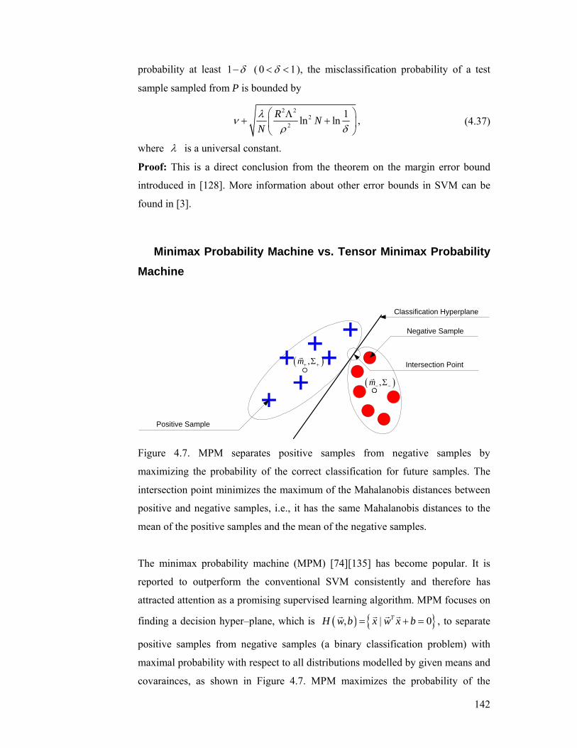
142
probability at least 1 δ− ( 0 1δ< < ), the misclassification probability of a test
sample sampled from P is bounded by
2 22
2
1ln lnR NNλν
ρ δ⎛ ⎞Λ
+ +⎜ ⎟⎝ ⎠
, (4.37)
where λ is a universal constant.
Proof: This is a direct conclusion from the theorem on the margin error bound
introduced in [128]. More information about other error bounds in SVM can be
found in [3].
Minimax Probability Machine vs. Tensor Minimax Probability Machine
Positive Sample
Negative Sample
Classification Hyperplane
( ),m+ +Σr
( ),m− −Σr
Intersection Point
Figure 4.7. MPM separates positive samples from negative samples by
maximizing the probability of the correct classification for future samples. The
intersection point minimizes the maximum of the Mahalanobis distances between
positive and negative samples, i.e., it has the same Mahalanobis distances to the
mean of the positive samples and the mean of the negative samples.
The minimax probability machine (MPM) [74][135] has become popular. It is
reported to outperform the conventional SVM consistently and therefore has
attracted attention as a promising supervised learning algorithm. MPM focuses on
finding a decision hyper–plane, which is ( ) { }, | 0TH w b x w x b= + =r r r r , to separate
positive samples from negative samples (a binary classification problem) with
maximal probability with respect to all distributions modelled by given means and
covarainces, as shown in Figure 4.7. MPM maximizes the probability of the
143
correct classification rate (classification accuracy) on future samples. For
Gaussian distributed samples, it minimizes the maximum of the Mahalanobis
distances of the positive samples and the negative samples. With given positive
samples ixr ( 1iy = + ) and negative samples ixr ( 1iy = − ), MPM is defined as,
( )
( ) ( ){ }
( ) ( ){ }
, ,
1 ~ ,
1 ~ ,
max , ,
inf Pr 0 s.t.
inf Pr 0i i
i i
MPMw b
Tix y m
Tix y m
J w b
w x b
w x b
δδ δ
δ
δ+ +
− −
=+ Σ
=− Σ
⎡ = ⎤⎢ ⎥⎢ ⎥+ ≥ ≥⎢ ⎥⎢ ⎥+ ≤ ≥⎢ ⎥⎣ ⎦
r
r r
r r
r
r r
r r
. (4.38)
Here, the notation ( ) ( )1 ,i ix y m+ += + Σr r means the class distribution of the
positive samples has the mean m+r and covariance +Σ , and similarly for the
notation ( ) ( )1 ,i ix y m− −= − Σr r . The classification decision function is given by
( ) sign Ty x w x b⎡ ⎤= +⎣ ⎦r r r .
Recently, based on the powerful Marshall and Olkin’s theorem [102], Popescu
and Bertsimas [120] proved a probability bound,
( ){ } 2
~ ,
1sup Pr1x m
x SdΣ
∈ =+r r
r with ( ) ( )2 1inf T
x Sd x m x m−
∈= − Σ −r
r r r r , (4.39)
where xr stands for a random vector, S is a given convex set, and the
supremum is taken over all distributions for xr with the mean value as mr and
the covariance matrix Σ . Based on this result, Lanckriet et al. [74] reformulated
(4.38) as:
( ), ,
max , ,
, 1 s.t.
, 1
MPMw b
T Ti
T Ti
J w b
w m b w w y
w m b w w y
κκ κ
κ
κ+ +
− −
=⎡ ⎤⎢ ⎥⎢ ⎥+ ≥ + Σ = +⎢ ⎥⎢ ⎥+ ≤ − Σ = −⎣ ⎦
r
r
r r r r
r r r r
, (4.40)
where the constraint functions in (4.40) are second order cone functions. There
MPM is an SOCP. This problem can be further simplified as
( )( )
min
s.t. 1
T TMPMwT
J w w w w w
w m m
+ −
+ −
⎡ ⎤= Σ + Σ⎢ ⎥⎢ ⎥− =⎣ ⎦
r
r r r r r
r r r , (4.41)
where b is determined by
( ) ( ) ( )( ) ( ) ( ) ( )
* ** *
* * * *
TT
T T
w wb w m
w w w w
++
+ −
Σ= −
Σ + Σ
r rr r
r r r r . (4.42)
144
In computer vision research, many objects are represented by tensors. To match
the input requirments in MPM, we need to vectorize the tensors to vectors. When
training samples are limited, the vectorization will be a disaster. This is because
MPM meets the matrix singular problem seriously (the ranks of +Σ and −Σ are
deficient). To reduce this problem, we propose the tensor extension of MPM, i.e.,
tensor MPM (TMPM). TMPM is a combination of MPM and STL.
Suppose we have training samples 1 2 ML L Li R × ×∈X L ( 1 i N≤ ≤ ) and their
corresponding class labels { }1, 1iy ∈ + − . The decision function is given by
( )1
signk
M
kk
y w b×=
⎡ ⎤= +⎢ ⎥
⎣ ⎦∏X X r . Projection vectors kL
kw R∈r (1 k M≤ ≤ ) and the
bias b in TMPM are obtained from
( )1
1| , ,
;11 1
;11 1
max | , ,
1 I( 1) sup s.t.
1 I( 1) sup
Mk k
k
k
MMPM k k
w b
MNT
i i k l l ll Mi k
MNT
i i k l l ll Mi k
J w b
y w b w wN
y w b w wN
κκ κ
κ
κ
==
× +≤ ≤= =+
× −≤ ≤= =−
⎡ ⎤=⎢ ⎥⎢ ⎥⎛ ⎞⎡ ⎤⎢ ⎥= + + ≥ + Σ⎜ ⎟⎢ ⎥⎢ ⎥⎣ ⎦⎝ ⎠⎢ ⎥
⎛ ⎞⎡ ⎤⎢ ⎥= − + ≤ − Σ⎜ ⎟⎢ ⎥⎢ ⎥⎣ ⎦⎝ ⎠⎣ ⎦
∑ ∏
∑ ∏
X
X
r
r
r r r
r r r
, (4.43)
where ;l+Σ is the covariance matrix of the projected samples ( )i l lw−×X r for all
1iy = + and ;l−Σ is the covariance matrix of the projected samples ( )i l lw−×X r
for all 1iy = − . The function I( 1)iy = + is 1 if iy is 1+ , otherwise 0. The
function I( 1)iy = − is 1 if iy is 1− , otherwise 0. This problem can be
simplified as
( )1
1| , ,
;11
;11
max | , ,
sup s.t.
sup
Mk k
k
k
MMPM k k
w b
MT
k l l ll Mk
MT
k l l ll Mk
J w b
w b w w
w b w w
κκ κ
κ
κ
==
+ × +≤ ≤=
− × −≤ ≤=
⎡ ⎤=⎢ ⎥⎢ ⎥⎢ ⎥+ ≥ + Σ⎢ ⎥⎢ ⎥⎢ ⎥+ ≤ − Σ⎢ ⎥⎣ ⎦
∏
∏
M
M
r
r
r r r
r r r
, (4.44)
where ( ) [ ]11 I( 1)N
i iiN y+ + =
= = +∑M X , ( ) [ ]11 I( 1)N
i iiN y− − =
= = −∑M X , and
N+ ( N− ) is the number of positive (negative) samples.
The Lagrangian for this problem is
145
( )1 1 ;11
2 ;11
1 21
1
| , , , sup
sup
k
k
k
MM T
k k k l l ll Mk
MT
k l l ll Mk
M
kk
L w b w b w w
w b w w
b b wN N
κ α κ α κ
α κ
α ακ α
= + × +≤ ≤=
− × −≤ ≤=
+ ×=+ −
⎛ ⎞= − − + − Σ⎜ ⎟
⎝ ⎠⎛ ⎞
+ + + Σ⎜ ⎟⎝ ⎠
= − − + −
∏
∏
∏
M
M
M
rr r r r
r r r
r2
1
1 2; ;
1 1 sup sup
k
M
kk
T Tl l l l l l
l M l M
w
w w w wN N
α
α κ α κ
− ×=
+ −≤ ≤ ≤ ≤+ −
+
+ Σ + Σ
∏M r
r r r r
(4.45)
with Lagrangian multipliers 0iα ≥ ( 1,2i = ). The solution is determined by the
saddle point of the Lagrangian
( )1
1| , ,
max min | , , ,M
k k
Mk k
w bL w b
α κκ α
==r r
rr . (4.46)
This can be achieved by setting 0jw L∂ =r , 0bL∂ = , and 0Lκ∂ = . It is not
difficult to find that the solution of jwr depends on kwr (1 k M≤ ≤ , k j≠ ).
Therefore, there is no closed form solution for TMPM. We use the proposed
alternating projection method in STL to obtain the solution of TMPM. To have
the alternating projection method for TMPM, we need to replace the Step 4 in
Table 4.1 by the following optimization problem,
( )
( )( )
, ,
;
;
max , ,
s.t.
jMPM jw b
T Tj j j j j j
T Tj j j j j j
J w b
w w b w w
w w b w w
κκ κ
κ
κ
+ +
− −
⎡ ⎤=⎢ ⎥⎢ ⎥
× + ≥ + Σ⎢ ⎥⎢ ⎥
× + ≤ − Σ⎢ ⎥⎣ ⎦
M
M
r
r
r r r r
r r r r
. (4.47)
This problem is the standard MPM defined in (4.40).
Fisher Discriminant Analysis vs. Tensor Fisher Discriminant Analysis
Fisher discriminant analysis (FDA) [37][30][69] has been widely applied for
classification. Suppose there are N training samples Lix R∈r ( 1 i N≤ ≤ )
associated with their class labels { }1, 1iy ∈ + − . There are N+ positive training
samples and their mean is ( ) [ ]11 I( 1)N
i iim N y x+ + =
= = +∑r r ; there are N−
negative training samples and their mean can be calculated from
( ) [ ]11 I( 1)N
i iim N y x− − =
= = −∑r r ; the mean of all training samples is
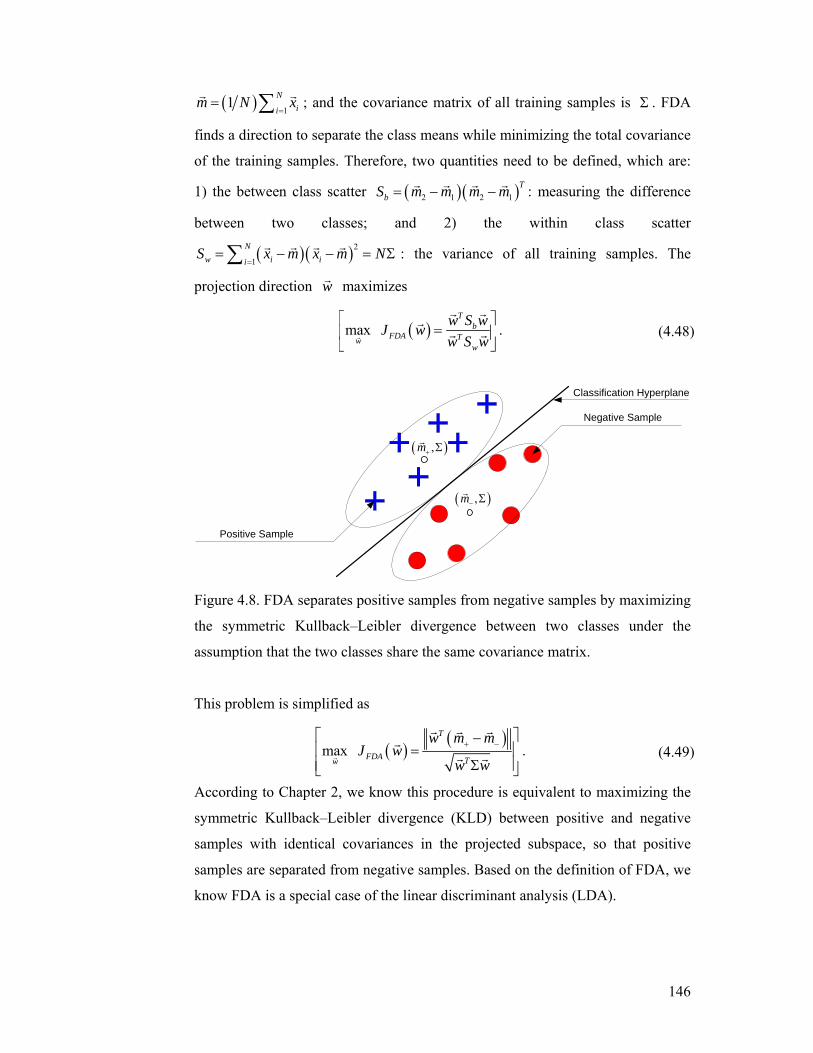
146
( ) 11 N
iim N x
== ∑r r ; and the covariance matrix of all training samples is Σ . FDA
finds a direction to separate the class means while minimizing the total covariance
of the training samples. Therefore, two quantities need to be defined, which are:
1) the between class scatter ( )( )2 1 2 1T
bS m m m m= − −r r r r : measuring the difference
between two classes; and 2) the within class scatter
( )( )2
1
Nw i ii
S x m x m N=
= − − = Σ∑ r r r r : the variance of all training samples. The
projection direction wr maximizes
( )max T
bFDA Tw
w
w S wJ ww S w
⎡ ⎤=⎢ ⎥
⎣ ⎦r
r rr
r r . (4.48)
Positive Sample
Negative Sample
Classification Hyperplane
( ),m+ Σr
( ),m− Σr
Figure 4.8. FDA separates positive samples from negative samples by maximizing
the symmetric Kullback–Leibler divergence between two classes under the
assumption that the two classes share the same covariance matrix.
This problem is simplified as
( )( )
max T
FDA Tw
w m mJ w
w w+ −
⎡ ⎤−⎢ ⎥=⎢ ⎥Σ⎣ ⎦
r
r r rr
r r . (4.49)
According to Chapter 2, we know this procedure is equivalent to maximizing the
symmetric Kullback–Leibler divergence (KLD) between positive and negative
samples with identical covariances in the projected subspace, so that positive
samples are separated from negative samples. Based on the definition of FDA, we
know FDA is a special case of the linear discriminant analysis (LDA).
147
The decision function in FDA is ( ) sign Ty x w x b⎡ ⎤= +⎣ ⎦r r r , where wr is the
eigenvector of ( )( )1 Tm m m m−+ − + −Σ − −r r r r associated with the largest eigenvalue
and the bias b is calculated by
( )TN N N m N m wb
N N− + + + − −
− +
− − +=
+
r r r
. (4.50)
The significance [30][39] of FDA is: FDA is Bayes optimal when the two classes
are Gaussian distributed with identical covariances.
When objects are represented by tensors, we need to vectorize the tensors to
vectors to match the input requirments in FDA. When training samples are
limited, the vectorization will be a disaster for FDA. This is because wS and bS
are both singular. To reduce this problem, we propose the tensor extension of
FDA, i.e., tensor FDA (TFDA). TFDA is a combination of FDA and STL.
Moreover, TFDA is a special case of the previous proposed general tensor
discriminant analysis (GTDA).
Suppose we have training samples 1 2 ML L Li R × ×∈X L ( 1 i N≤ ≤ ) and their
corresponding class labels { }1, 1iy ∈ + − . The mean of the positive training
samples is ( ) [ ]11 I( 1)N
i iiN y+ + =
= = +∑M X ; the mean of the negative training
samples is ( ) [ ]11 I( 1)N
i iiN y− − =
= = −∑M X ; the mean of all training samples is
( ) 11 N
iiN
== ∑M X ; and N+ ( N− ) is the number of positive (negative) samples.
The decision function is defined by ( )1
signk
M
kk
y w b×=
⎡ ⎤= +⎢ ⎥
⎣ ⎦∏X X r , where the
projection vectors kLkw R∈r (1 k M≤ ≤ ) and the bias b in TFDA are obtained
from
( )( )
( )1
2
11 2|
1 1
max |k
Mk k
k
M
kkM
TFDA k k MNw
i ki k
wJ w
w=
+ − ×=
=
×= =
⎡ ⎤−⎢ ⎥
⎢ ⎥=⎢ ⎥⎢ ⎥−⎢ ⎥⎣ ⎦
∏
∑ ∏
M M
X Mr
r
r
r, (4.51)
The formula is obtained directly from (3.31) and (3.32). Similar to GTDA, there is
no closed form solution for TFDA. The alternating projection is applied to obtain
the solution for TFDA and we need to replace the Step 4 in Table 4.1 by the
following optimization problem,
148
( ) ( )
( )
2
2
1
max j
Tj j j
TFDA j Nw Tj i j j
i
w wJ w
w w
+ −
=
⎡ ⎤⎢ ⎥⎡ ⎤− ×⎣ ⎦⎢ ⎥=⎢ ⎥⎡ ⎤− ×⎣ ⎦⎢ ⎥⎣ ⎦
∑
M M
X Mr
r rr
r r. (4.52)
This problem is the standard FDA. When we have the projection vectors 1|Mk kw =r ,
we can obtain the bias b from
( )1
k
M
kk
N N N N wb
N N
− + + + − − ×=
− +
− − +=
+
∏M M r
. (4.53)
Distance Metric Learning vs. Multiple Distance Metrics Learning
Weinberger et al. [169] proposed the distance metric learning (DML) to learn a
metric for k–nearest–neighbor (kNN) classification. The motivation of DML is
simple because the performance of kNN is only related to the metric used for
dissimilarity measure. In traditional kNN, the Euclidean metric fails to capture the
statistical charateristics of training samples. In DML, the metric is obtained such
that “k–nearest neighbors always belong to the same class while examples from
different classes are separated by a large margin”. DML is defined by
( ) ( ) ( ) ( )
( ) ( ) ( ) ( )
, 1 1 1 11 , ,
min , 1
1 , 1 , ,
s.t. 0,
ijl
N N N NT
DML ijl ij i j i j ij il ijli j i ji j l N
TTi l i l i j i j ijl
ijl
J x x x x c y
x x x x x x x x i j l N
ξξ η η ξ
ξ
ξ
Σ= = = =≤ ≤
Σ = − Σ − + −
− Σ − − − Σ − ≥ − ≤ ≤
≥
∑∑ ∑∑r r r r
r r r r r r r r
1 , ,0
i j l N
⎡ ⎤⎢ ⎥⎢ ⎥⎢ ⎥⎢ ⎥⎢ ⎥≤ ≤⎢ ⎥⎢ ⎥Σ ≥⎣ ⎦
(4.54)
where 1ijη = and 1ijy = mean that ixr and jxr have the same class label,
otherwise 0. The constraint function 0Σ ≥ indicates that the maxtrix Σ is
required to be positive semidefinite, so the problem is an SDP. From the learnt
distance metric Σ , it is direct to have the linear transformation matrix by
decomposing TW WΣ = .
The optimization problem defined in (4.54) is equivalent to
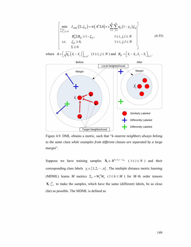
149
( ) ( ) ( ), 1 11 , ,
min , tr 1
1 , 1 , , s.t. 0, 1 , ,
0
ijl
N NT
DML ijl ij il ijli ji j l N
Tijl ijl ijl
ijl
J A A c y
B B i j l Ni j l N
ξξ η ξ
ξξ
Σ= =≤ ≤
Σ = Σ + −
Σ ≥ − ≤ ≤≥ ≤ ≤
Σ ≥
∑∑
⎡ ⎤⎢ ⎥⎢ ⎥⎢ ⎥⎢ ⎥⎢ ⎥⎢ ⎥⎣ ⎦
(4.55)
where ( ) 2ij i j L NA x xη
×⎡ ⎤= −⎣ ⎦
r r (1 ,i j N≤ ≤ ) and 2
,ijl i l j i LB x x x x
×⎡ ⎤= − −⎣ ⎦r r r r .
Margin Margin
Target Neighborhood
Local NeighborhoodBefore After
ixr
ixr
Similarly Labeled
Differently Labeled
Differently Labeled
Figure 4.9. DML obtains a metric, such that “k–nearest neighbors always belong
to the same class while examples from different classes are separated by a large
margin”.
Suppose we have training samples 1 2 ML L Li R × ×∈X L ( 1 i N≤ ≤ ) and their
corresponding class labels { }1, 2, ,iy n∈ L . The multiple distance metric learning
(MDML) learns M metrics Tk k kW WΣ = ( 1 k M≤ ≤ ) for M–th order tensors
1|Ni i=X to make the samples, which have the same (different) labels, be as close
(far) as possible. The MDML is defined as
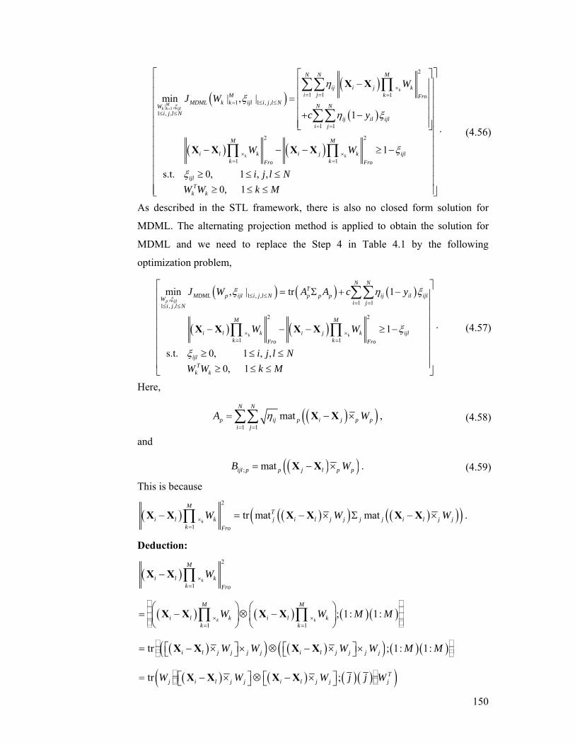
150
( )( )
( )
( ) ( )
1
2
1 1 11 1 , ,
| ,1 , ,
1 1
2 2
1 1
min | , |1
1
s.t. 0, 1 , ,
k
Mk k ijl
k k
MN N
ij i j ki j kM Fro
MDML k k ijl i j l N N NWi j l N
ij il ijli j
M M
i l k i j k ijlk kFro Fro
ijl
WJ W
c y
W W
i j l N
ξ
ηξ
η ξ
ξ
ξ
=
×= = =
= ≤ ≤
≤ ≤
= =
× ×= =
⎡ ⎤−⎢ ⎥
⎢ ⎥= ⎢ ⎥⎢ ⎥+ −⎢ ⎥⎣ ⎦
− − − ≥ −
≥ ≤ ≤
∑∑ ∏
∑∑
∏ ∏
X X
X X X X
0, 1 T
k kW W k M
⎡ ⎤⎢ ⎥⎢ ⎥⎢ ⎥⎢ ⎥⎢ ⎥⎢ ⎥⎢ ⎥⎢ ⎥⎢ ⎥⎢ ⎥⎢ ⎥
≥ ≤ ≤⎢ ⎥⎣ ⎦
. (4.56)
As described in the STL framework, there is also no closed form solution for
MDML. The alternating projection method is applied to obtain the solution for
MDML and we need to replace the Step 4 in Table 4.1 by the following
optimization problem,
( ) ( ) ( )
( ) ( )
1 , ,, 1 11 , ,
2 2
1 1
min , | tr 1
1
s.t. 0, 1 , ,
p ijl
k k
N NT
MDML p ijl i j l N p p p ij il ijlW i ji j l N
M M
i l k i j k ijlk kFro Fro
ijl
J W A A c y
W W
i j l NW
ξξ η ξ
ξ
ξ
≤ ≤= =≤ ≤
× ×= =
= Σ + −
− − − ≥ −
≥ ≤ ≤
∑∑
∏ ∏X X X X
0, 1 Tk kW k M
⎡ ⎤⎢ ⎥⎢ ⎥⎢ ⎥⎢ ⎥⎢ ⎥⎢ ⎥⎢ ⎥⎢ ⎥≥ ≤ ≤⎣ ⎦
. (4.57)
Here,
( )( )1 1
matN N
p ij p i j p pi j
A Wη= =
= − ×∑∑ X X , (4.58)
and
( )( ); matijl p p j l p pB W= − ×X X . (4.59)
This is because
( ) ( )( ) ( )( )( )2
1
tr mat matk
MT
i l k j i l j j j j i l j jk Fro
W W W×=
− = − × Σ − ×∏X X X X X X .
Deduction:
( )2
1k
M
i l kk Fro
W×=
− ∏X X
( ) ( ) ( )( )1 1
; 1: 1:k k
M M
i l k i l kk k
W W M M× ×= =
⎛ ⎞ ⎛ ⎞= − ⊗ −⎜ ⎟ ⎜ ⎟
⎝ ⎠ ⎝ ⎠∏ ∏X X X X
( )( ) ( )( ) ( )( )tr ; 1: 1:i l j j j j i l j j j jW W W W M M⎡ ⎤ ⎡ ⎤= − × × ⊗ − × ×⎣ ⎦ ⎣ ⎦X X X X
( ) ( ) ( )( )( )tr ; Tj i l j j i l j j jW W W j j W⎡ ⎤ ⎡ ⎤= − × ⊗ − ×⎣ ⎦ ⎣ ⎦X X X X

151
( )( ) ( )( )( )tr mat matT Tj j i l j j j i l j j jW W W W= − × − ×X X X X
( )( ) ( )( )( )tr mat matT Tj i l j j j j j i l j jW W W W= − × − ×X X X X
( )( ) ( )( )( )tr mat mat .Tj i l j j j j i l j jW W= − × Σ − ×X X X X
This problem defined in (4.57) is the standard DML.
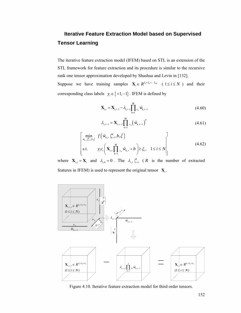
152
Iterative Feature Extraction Model based on Supervised Tensor Learning
The iterative feature extraction model (IFEM) based on STL is an extension of the
STL framework for feature extraction and its procedure is similar to the recursive
rank one tensor approximation developed by Shashua and Levin in [132].
Suppose we have training samples 1 2 ML L Li R × ×∈X L ( 1 i N≤ ≤ ) and their
corresponding class labels { }1, 1iy ∈ + − . IFEM is defined by
, , 1 , 1 , 11
k
M
i r i r i r k rk
wλ− − × −=
= − ∏X X r (4.60)
( ), 1 , 1 , 11
k
M T
i r i r k rk
wλ − − × −=
= ∏X r (4.61)
( ), 1
, 1| , ,
, ,1
min | , ,
s.t. , 1
Mk r k
k
Mk r k
w b
M
i i i r k r ik
f w b
y c w b i N
ξξ
ξ
==
×=
⎡ ⎤⎢ ⎥⎢ ⎥⎛ ⎞⎢ ⎥+ ≥ ≤ ≤⎜ ⎟⎢ ⎥⎝ ⎠⎣ ⎦
∏X
rr
rr
r (4.62)
where ,1i i=X X and ,0 0iλ = . The , 1|Ri r rλ = ( R is the number of extracted
features in IFEM) is used to represent the original tensor iX .
1 2 3, 1
(1 )
L L Li r R
i N
× ×− ∈
≤ ≤
X
1 2 3, 1
(1 )
L L Li r R
i N
× ×− ∈
≤ ≤
X 3
, 1 , 11
i r k rk
wλ − ⊗ −=∏ r 1 2 3
,
(1 )
L L Li r R
i N
× ×∈
≤ ≤
X
2, 1rw −r
1×
3×
2×2, 1rw −r, 1i tλ −
Figure 4.10. Iterative feature extraction model for third order tensors.
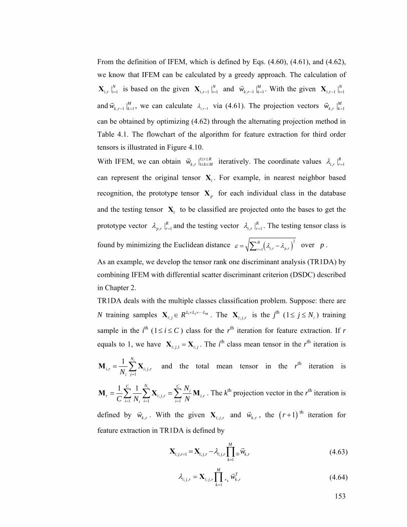
153
From the definition of IFEM, which is defined by Eqs. (4.60), (4.61), and (4.62),
we know that IFEM can be calculated by a greedy approach. The calculation of
, 1|Ni r i=X is based on the given , 1 1|Ni r i− =X and , 1 1|Mk r kw − =
r . With the given , 1 1|Ni r i− =X
and , 1 1|Mk r kw − =r , we can calculate , 1i rλ − via (4.61). The projection vectors , 1|Mk r kw =
r
can be obtained by optimizing (4.62) through the alternating projection method in
Table 4.1. The flowchart of the algorithm for feature extraction for third order
tensors is illustrated in Figure 4.10.
With IFEM, we can obtain 1, 1|
r Rk r k Mw ≤ ≤
≤ ≤r iteratively. The coordinate values , 1|Ri r rλ =
can represent the original tensor iX . For example, in nearest neighbor based
recognition, the prototype tensor pX for each individual class in the database
and the testing tensor tX to be classified are projected onto the bases to get the
prototype vector , 1|Rp r rλ = and the testing vector , 1|Rt r rλ = . The testing tensor class is
found by minimizing the Euclidean distance ( )2
, ,1
Rt r p rr
ε λ λ=
= −∑ over p .
As an example, we develop the tensor rank one discriminant analysis (TR1DA) by
combining IFEM with differential scatter discriminant criterion (DSDC) described
in Chapter 2.
TR1DA deals with the multiple classes classification problem. Suppose: there are
N training samples 1 2;
ML L Li j R × ×∈X L . The ; ,i j rX is the jth (1 ij N≤ ≤ ) training
sample in the ith (1 i C≤ ≤ ) class for the rth iteration for feature extraction. If r
equals to 1, we have ; ,1 ;i j i j=X X . The ith class mean tensor in the rth iteration is
, ; ,1
1 iN
i r i j rjiN =
= ∑M X and the total mean tensor in the rth iteration is
; , ,1 1 1
1 1 iNC Ci
r i j r i ri i ii
NC N N= = =
= =∑ ∑ ∑M X M . The kth projection vector in the rth iteration is
defined by ,k rwr . With the given ; ,i j rX and ,k rwr , the ( )1r + th iteration for
feature extraction in TR1DA is defined by
; , 1 ; , ; , ,1
M
i j r i j r i j r k rk
wλ+ ⊗=
= − ∏X X r (4.63)
; , ; , ,1
k
MT
i j r i j r k rk
wλ ×=
= ∏X r (4.64)
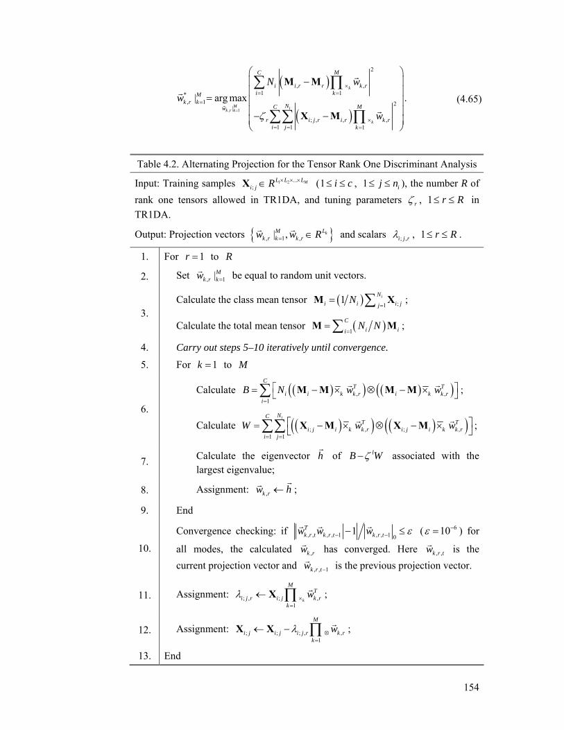
154
( )
( ), 1
2
, ,1 1*
, 1 2|
; , , ,1 1 1
| arg maxk
M ik r k
k
MC
i i r r k ri kM
k r kN MCw
r i j r i r k ri j k
N ww
wζ=
×= =
=
×= = =
⎛ ⎞−⎜ ⎟
⎜ ⎟= ⎜ ⎟⎜ ⎟− −⎜ ⎟⎝ ⎠
∑ ∏
∑∑ ∏
M M
X Mr
r
r
r. (4.65)
Table 4.2. Alternating Projection for the Tensor Rank One Discriminant Analysis
Input: Training samples 1 2 ...;
ML L Li j R × × ×∈X (1 i c≤ ≤ , 1 ij n≤ ≤ ), the number R of
rank one tensors allowed in TR1DA, and tuning parameters rζ , 1 r R≤ ≤ in TR1DA.
Output: Projection vectors { }, 1 ,| , kLMk r k k rw w R= ∈r r and scalars ; ,i j rλ , 1 r R≤ ≤ .
1. For 1r = to R
2. Set , 1|Mk r kw =r be equal to random unit vectors.
3. Calculate the class mean tensor ( ) ;1
1 iNi i i jj
N=
= ∑M X ;
Calculate the total mean tensor ( )1
Ci ii
N N=
=∑M M ;
4. Carry out steps 5–10 iteratively until convergence.
5. For 1k = to M
6.
Calculate ( )( ) ( )( ), ,1
CT T
i i k k r i k k ri
B N w w=
⎡ ⎤= − × ⊗ − ×⎣ ⎦∑ M M M Mr r ;
Calculate ( )( ) ( )( ); , ; ,1 1
iNCT T
i j i k k r i j i k k ri j
W w w= =
⎡ ⎤= − × ⊗ − ×⎣ ⎦∑∑ X M X Mr r ;
7. Calculate the eigenvector hr
of lB Wζ− associated with the largest eigenvalue;
8. Assignment: ,k rw h←rr ;
9. End
10.
Convergence checking: if , , , , 1 , , 1 01T
k r t k r t k r tw w w ε− −− ≤r r r ( 610ε −= ) for
all modes, the calculated ,k rwr has converged. Here , ,k r twr is the current projection vector and , , 1k r tw −
r is the previous projection vector.
11. Assignment: ; , ; ,1
k
MT
i j r i j k rk
wλ ×=
← ∏X r ;
12. Assignment: ; ; ; , ,1
M
i j i j i j r k rk
wλ ⊗=
← − ∏X X r ;
13. End
155
The algorithm is given in Table 4.2.
The time complexity of PCA (LDA) is ( )3
1
Mkk
O L=
⎛ ⎞⎜ ⎟⎝ ⎠∏ when training samples
X belong to 1 2 ML L LR × × ×L . The time complexity of TR1DA is
( )1 1
R Mr kr k
O T L= =∑ ∑ , where rT is the number of iterations to make TR1DA
converge for the rth feature extraction procedure (in our experiments for human
gait recognition [143][145], rT is about 20). The space complexity of PCA
(LDA) is ( )2
1
Mkk
O L=
⎛ ⎞⎜ ⎟⎝ ⎠∏ . The space complexity of TR1DA is ( )1
Mkk
O L=∏ .
This indicates that the time complexity and the space complexity of feature
extraction are reduced by working directly with tensor data rather than vectorizing
the data and applying PCA (LDA).
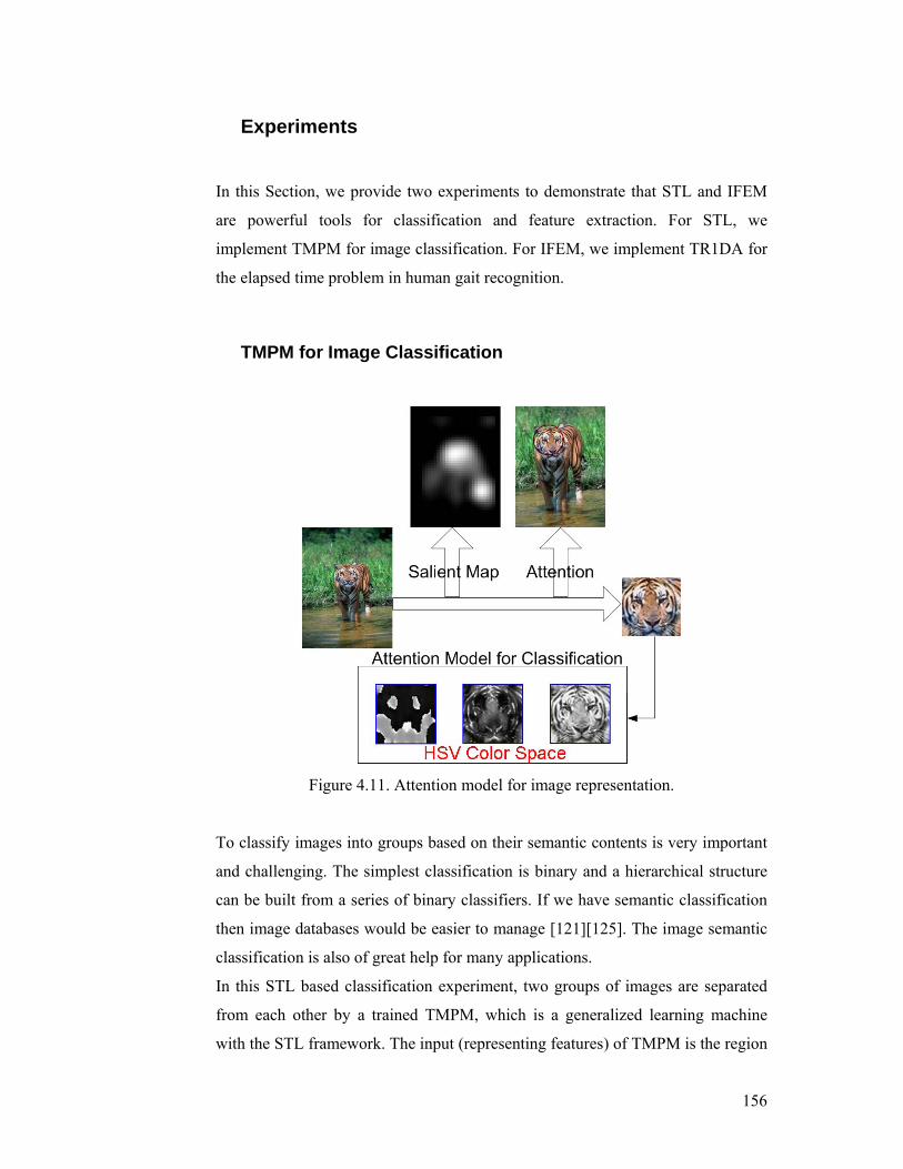
156
Experiments
In this Section, we provide two experiments to demonstrate that STL and IFEM
are powerful tools for classification and feature extraction. For STL, we
implement TMPM for image classification. For IFEM, we implement TR1DA for
the elapsed time problem in human gait recognition.
TMPM for Image Classification
Figure 4.11. Attention model for image representation.
To classify images into groups based on their semantic contents is very important
and challenging. The simplest classification is binary and a hierarchical structure
can be built from a series of binary classifiers. If we have semantic classification
then image databases would be easier to manage [121][125]. The image semantic
classification is also of great help for many applications.
In this STL based classification experiment, two groups of images are separated
from each other by a trained TMPM, which is a generalized learning machine
with the STL framework. The input (representing features) of TMPM is the region
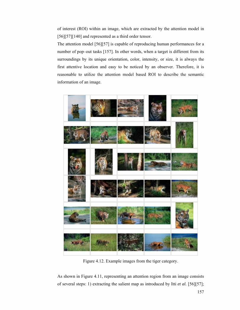
157
of interest (ROI) within an image, which are extracted by the attention model in
[56][57][140] and represented as a third order tensor.
The attention model [56][57] is capable of reproducing human performances for a
number of pop–out tasks [157]. In other words, when a target is different from its
surroundings by its unique orientation, color, intensity, or size, it is always the
first attentive location and easy to be noticed by an observer. Therefore, it is
reasonable to utilize the attention model based ROI to describe the semantic
information of an image.
Figure 4.12. Example images from the tiger category.
As shown in Figure 4.11, representing an attention region from an image consists
of several steps: 1) extracting the salient map as introduced by Itti et al. [56][57];
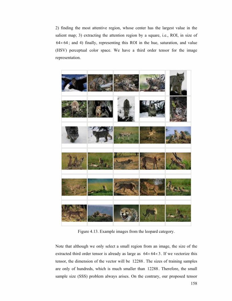
158
2) finding the most attentive region, whose center has the largest value in the
salient map; 3) extracting the attention region by a square, i.e., ROI, in size of
64 64× ; and 4) finally, representing this ROI in the hue, saturation, and value
(HSV) perceptual color space. We have a third order tensor for the image
representation.
Figure 4.13. Example images from the leopard category.
Note that although we only select a small region from an image, the size of the
extracted third order tensor is already as large as 64 64 3× × . If we vectorize this
tensor, the dimension of the vector will be 12288 . The sizes of training samples
are only of hundreds, which is much smaller than 12288 . Therefore, the small
sample size (SSS) problem always arises. On the contrary, our proposed tensor
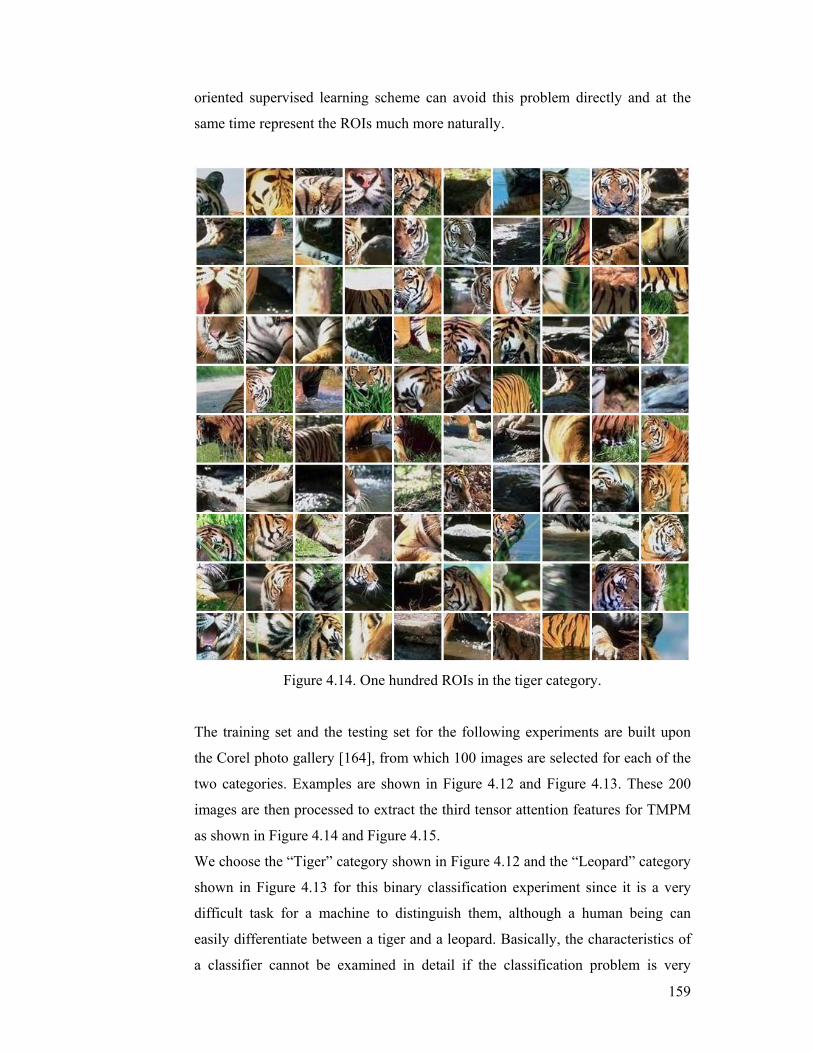
159
oriented supervised learning scheme can avoid this problem directly and at the
same time represent the ROIs much more naturally.
Figure 4.14. One hundred ROIs in the tiger category.
The training set and the testing set for the following experiments are built upon
the Corel photo gallery [164], from which 100 images are selected for each of the
two categories. Examples are shown in Figure 4.12 and Figure 4.13. These 200
images are then processed to extract the third tensor attention features for TMPM
as shown in Figure 4.14 and Figure 4.15.
We choose the “Tiger” category shown in Figure 4.12 and the “Leopard” category
shown in Figure 4.13 for this binary classification experiment since it is a very
difficult task for a machine to distinguish them, although a human being can
easily differentiate between a tiger and a leopard. Basically, the characteristics of
a classifier cannot be examined in detail if the classification problem is very
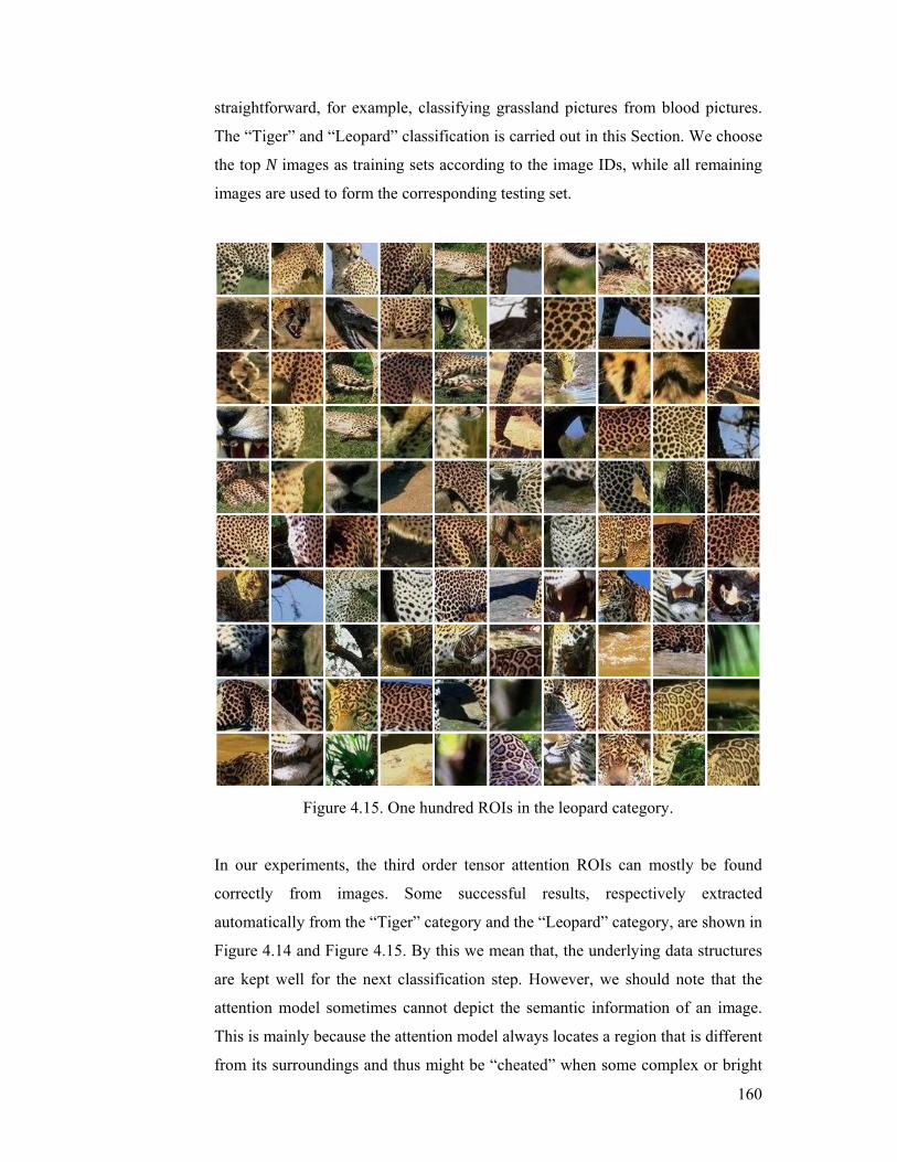
160
straightforward, for example, classifying grassland pictures from blood pictures.
The “Tiger” and “Leopard” classification is carried out in this Section. We choose
the top N images as training sets according to the image IDs, while all remaining
images are used to form the corresponding testing set.
Figure 4.15. One hundred ROIs in the leopard category.
In our experiments, the third order tensor attention ROIs can mostly be found
correctly from images. Some successful results, respectively extracted
automatically from the “Tiger” category and the “Leopard” category, are shown in
Figure 4.14 and Figure 4.15. By this we mean that, the underlying data structures
are kept well for the next classification step. However, we should note that the
attention model sometimes cannot depict the semantic information of an image.
This is mainly because the attention model always locates a region that is different
from its surroundings and thus might be “cheated” when some complex or bright
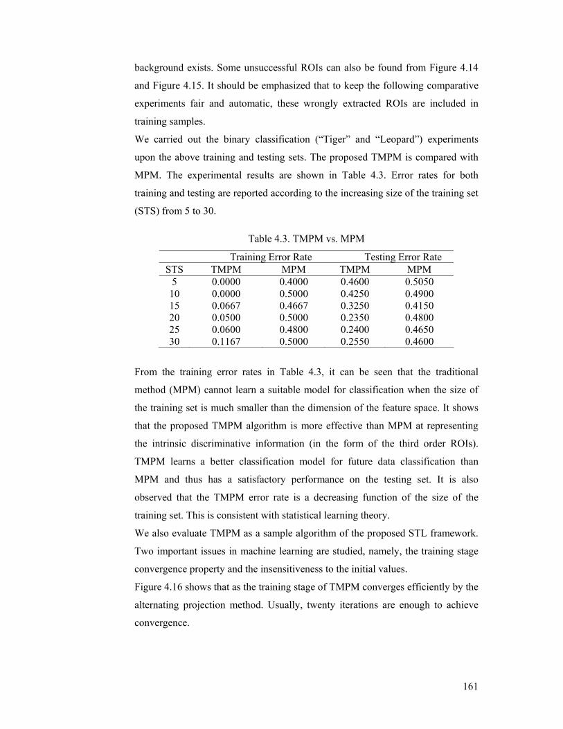
161
background exists. Some unsuccessful ROIs can also be found from Figure 4.14
and Figure 4.15. It should be emphasized that to keep the following comparative
experiments fair and automatic, these wrongly extracted ROIs are included in
training samples.
We carried out the binary classification (“Tiger” and “Leopard”) experiments
upon the above training and testing sets. The proposed TMPM is compared with
MPM. The experimental results are shown in Table 4.3. Error rates for both
training and testing are reported according to the increasing size of the training set
(STS) from 5 to 30.
Table 4.3. TMPM vs. MPM
Training Error Rate Testing Error Rate STS TMPM MPM TMPM MPM
5 0.0000 0.4000 0.4600 0.5050 10 0.0000 0.5000 0.4250 0.4900 15 0.0667 0.4667 0.3250 0.4150 20 0.0500 0.5000 0.2350 0.4800 25 0.0600 0.4800 0.2400 0.4650 30 0.1167 0.5000 0.2550 0.4600
From the training error rates in Table 4.3, it can be seen that the traditional
method (MPM) cannot learn a suitable model for classification when the size of
the training set is much smaller than the dimension of the feature space. It shows
that the proposed TMPM algorithm is more effective than MPM at representing
the intrinsic discriminative information (in the form of the third order ROIs).
TMPM learns a better classification model for future data classification than
MPM and thus has a satisfactory performance on the testing set. It is also
observed that the TMPM error rate is a decreasing function of the size of the
training set. This is consistent with statistical learning theory.
We also evaluate TMPM as a sample algorithm of the proposed STL framework.
Two important issues in machine learning are studied, namely, the training stage
convergence property and the insensitiveness to the initial values.
Figure 4.16 shows that as the training stage of TMPM converges efficiently by the
alternating projection method. Usually, twenty iterations are enough to achieve
convergence.
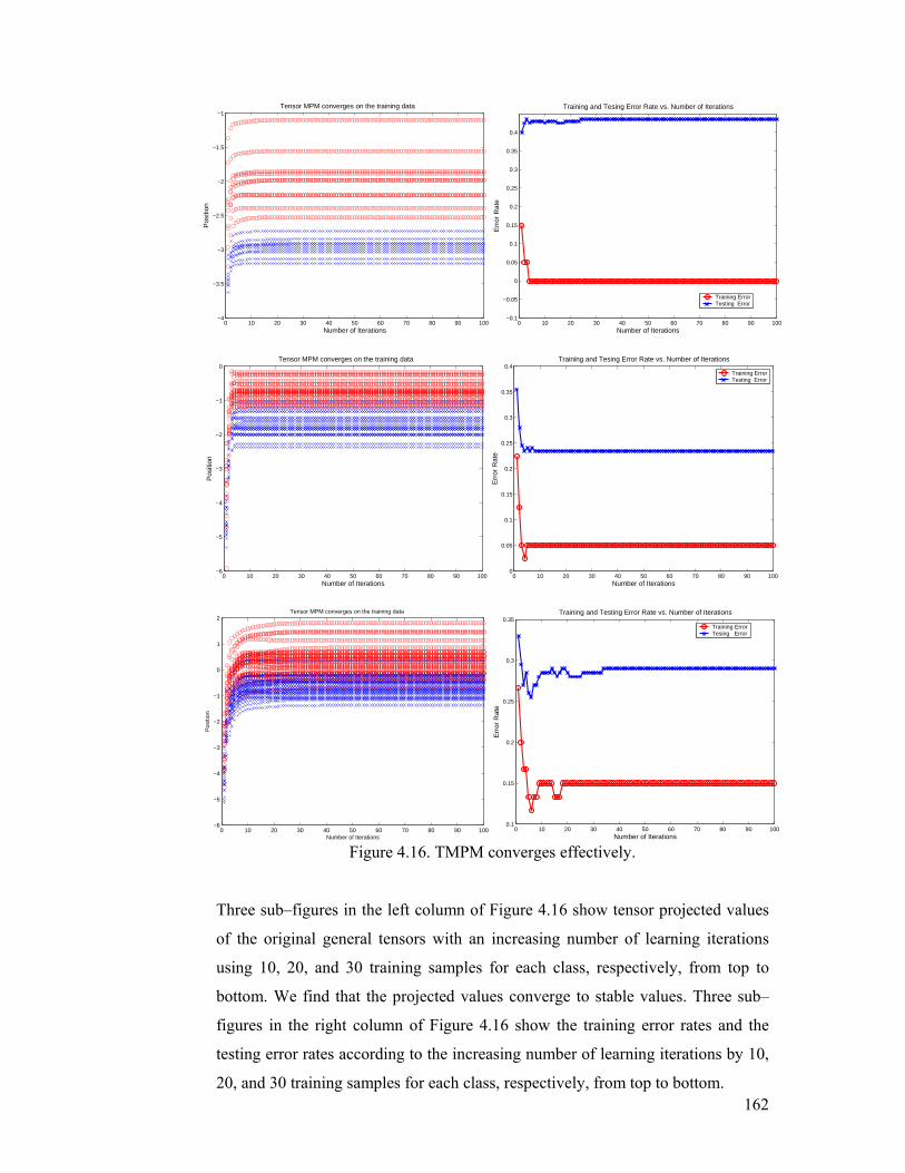
162
0 10 20 30 40 50 60 70 80 90 100−4
−3.5
−3
−2.5
−2
−1.5
−1
Number of Iterations
Pos
ition
Tensor MPM converges on the training data
0 10 20 30 40 50 60 70 80 90 100−0.1
−0.05
0
0.05
0.1
0.15
0.2
0.25
0.3
0.35
0.4
Number of Iterations
Err
or R
ate
Training and Tesing Error Rate vs. Number of Iterations
Training ErrorTesting Error
0 10 20 30 40 50 60 70 80 90 100−6
−5
−4
−3
−2
−1
0
Number of Iterations
Pos
ition
Tensor MPM converges on the training data
0 10 20 30 40 50 60 70 80 90 1000
0.05
0.1
0.15
0.2
0.25
0.3
0.35
0.4
Number of Iterations
Err
or R
ate
Training and Tesing Error Rate vs. Number of Iterations
Training ErrorTesting Error
0 10 20 30 40 50 60 70 80 90 100−6
−5
−4
−3
−2
−1
0
1
2
Number of Iterations
Pos
ition
Tensor MPM converges on the training data
0 10 20 30 40 50 60 70 80 90 1000.1
0.15
0.2
0.25
0.3
0.35
Number of Iterations
Err
or R
ate
Training and Testing Error Rate vs. Number of Iterations
Training ErrorTesing Error
Figure 4.16. TMPM converges effectively.
Three sub–figures in the left column of Figure 4.16 show tensor projected values
of the original general tensors with an increasing number of learning iterations
using 10, 20, and 30 training samples for each class, respectively, from top to
bottom. We find that the projected values converge to stable values. Three sub–
figures in the right column of Figure 4.16 show the training error rates and the
testing error rates according to the increasing number of learning iterations by 10,
20, and 30 training samples for each class, respectively, from top to bottom.
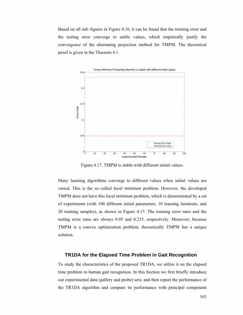
163
Based on all sub–figures in Figure 4.16, it can be found that the training error and
the testing error converge to stable values, which empirically justify the
convergence of the alternating projection method for TMPM. The theoretical
proof is given in the Theorem 4.1.
0 10 20 30 40 50 60 70 80 90 1000
0.05
0.1
0.15
0.2
0.25
Experimental Rounds
Erro
r Rat
e
Tensor Minimax Probability Machine is stable with different initial values
Testing Error RateTraining Error Rate
Figure 4.17. TMPM is stable with different initial values.
Many learning algorithms converge to different values when initial values are
varied. This is the so–called local minimum problem. However, the developed
TMPM does not have this local minimum problem, which is demonstrated by a set
of experiments (with 100 different initial parameters, 10 learning iterations, and
20 training samples), as shown in Figure 4.17. The training error rates and the
testing error rates are always 0.05 and 0.235, respectively. Moreover, because
TMPM is a convex optimization problem, theoretically TMPM has a unique
solution.
TR1DA for the Elapsed Time Problem in Gait Recognition
To study the characteristics of the proposed TR1DA, we utilize it on the elapsed
time problem in human gait recognition. In this Section we first briefly introduce
our experimental data (gallery and probe) sets; and then report the performance of
the TR1DA algorithm and compare its performance with principal component
164
analysis (PCA), linear discriminant analysis (LDA) and tensor rank one analysis
(TR1A). The experiments provide numerical evidence for the convergence of
TR1DA during the learning stage.
Research efforts in biometrics are mainly motivated by the increasing
requirements of machine based automatic human authentication/authorization
[71]. As a promising biometric source, human gait describes the manner of a
person’s walking and can be acquired at a distance. It was first analyzed in
medical surgery [111][112], and then in psychology [23]. In computer vision,
human motion has been studied for years [1]. An early attempt to recognize a
person by the gait was probably made by Little and Boyd [86]. Since then, many
efforts have been made for gait recognition [9][22][63][163]. In this Section, we
focus on an appearance based model, which could be a preprocessing step for
statistical models, such as Hidden Markov Model [65][66].
Our experiments are all carried out on the USF HumanID outdoor gait database
[126], which consists of the following covariates: change in viewpoints (Left/L or
Right/R), change in shoe types (A or B), change in walking surface (Grass/G or
Concrete/C), change in carrying conditions (Briefcase/B or No Briefcase/NB),
and elapsed time (May or November) between sequences being compared. The
detailed description about the database is given in §3.1.
Among all five covariates, elapsed time is our main concern in this Section
because human identification systems are normally required to work over long
periods of time. In this thesis, the remaining three conditions are examined
thoroughly, namely change in shoe types (A or B), change in walking surface
(Grass or Concrete), and change in carrying conditions (carrying a Briefcase or
No Briefcase). Consequently, we choose our gallery set (May, C, A, L, NB) from
the May data and consider eight pattern classification problems with the test sets
of CAL (Nov., C, A, L, NB), CBL (Nov., C, B, L, NB) , GAL (Nov., G, A, L,
NB), GBL (Nov., G, B, L, NB), CBAL (Nov., C, A, L, BF), CBBL (Nov., C, B,
L, BF), GBAL (Nov., G, A, L, BF), and GBBL (Nov., G, B, L, BF).
In this Section we empirically study the TR1DA approach in terms of accuracy,
convergence during the learning phase, and impact of parameter values on
accuracy. TR1DA is compared with existing methods, including PCA, LDA, and
TR1A. Experiments are carried out to recognize a gait with given examples of
165
gaits collected in the past (the elapsed time problem), which is still one of the
most difficult problems in human gait recognition.
In these experiments, we use EigenGait in a PCA based method for gait
recognition, FisherGait in an LDA based method [45], TR1AGait in a TR1A for
gait recognition, and TR1DAGait in a TR1DA for gait recognition. Figure 4.18
shows the first ten EigenGaits, FisherGaits, TR1AGaits, and TR1DAGaits,
respectively. We believe that TR1DA is a good method for classifying gaits
because our experiments support this belief. First, TR1DAGait usually performs
better than existing methods (EigenGait, FisherGait, and TR1AGait) in
recognition tasks. Second, the training procedure for TR1DA converges within
about 20 iterations. Third, it is not difficult to obtain a reasonable good
performance of TR1DA by adjusting the tuning parameters rς (1 r R≤ ≤ ). This
is because there is a wide range of values for rς , over which TR1DA achieves a
good performance. In our experiments, although we extract R features, given
R independent tuning parameters, we set all tuning parameters be equal to each
other, in order to reduce the number of parameters. It is possible to achieve better
performance if the values of the tuning parameters are allowed to be different.
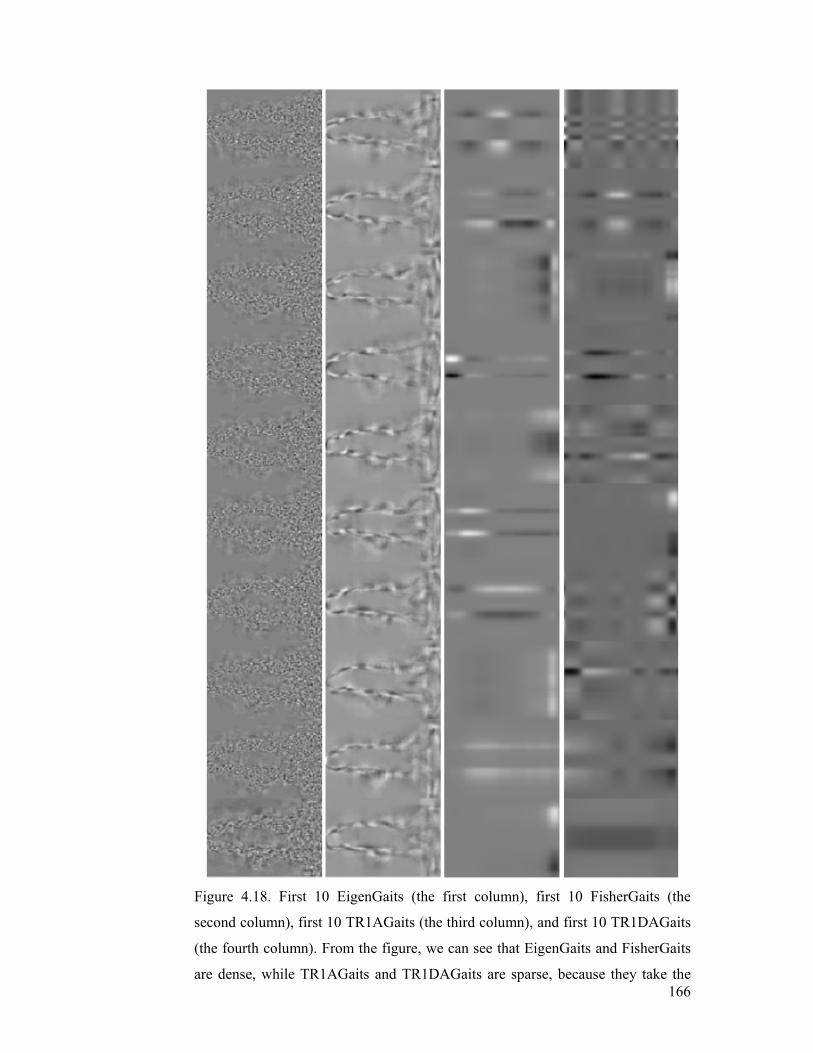
166
Figure 4.18. First 10 EigenGaits (the first column), first 10 FisherGaits (the
second column), first 10 TR1AGaits (the third column), and first 10 TR1DAGaits
(the fourth column). From the figure, we can see that EigenGaits and FisherGaits
are dense, while TR1AGaits and TR1DAGaits are sparse, because they take the
167
structure information into account to reduce the number of unknown parameters
in discriminant learning.
Figure 4.19–Figure 4.26 illustrate the experimental results under eight different
circumstances. In each of them:
• The first sub–figure shows the effects of feature dimension on recognition
precision (one minus the error rate). In this sub–figure, the x–coordinate is
the feature dimension and the y–coordinate is the recognition precision. In
order to keep the graph be in a manageable size, we only show the results
for feature dimensions from 10 to 110. In these experiments, we show the
top–one recognition precisions of EigenGait, FisherGait, TR1AGait, and
TR1DAGait. We show the top–one and top–five recognition precisions of
these algorithms in Table 4.5 and Table 4.6, respectively. Usually, tensor
based algorithms (TR1AGait and TR1DAGait) achieve better recognition
precisions than vector based algorithms (EigenGait and FisherGait) and
TR1DAGait performs better than TR1AGait.
• The second sub–figure shows the effects of feature dimension and the
tuning parameter ς on the recognition precision in TR1DA. In this sub–
figure, the x–coordinate is the feature dimension; the y–coordinate is the
tuning parameter ς ; and the z–coordinate is the recognition precision.
The feature dimension changes from 10 to 200 with a step 1 and ς
changes from 0.01 to 0.5 with a step 0.01. For each probe the tuning
parameter ς is chosen to achieve the best performance. The detailed
information about the value of ς is given in Table 4.4. In each case there
is a range of values of ς for which TR1DA achieves a good
performance. We only show one value for each probe. It can be observed
from the sub–figure that for each probe, there are a number of points to
achieve the best performance according to different ς values.
• The third sub–figure shows the number of iterations required in the
training procedure for extracting the ith feature. In this sub–figure, the x–
coordinate is the feature dimension and the y–coordinate is the number of
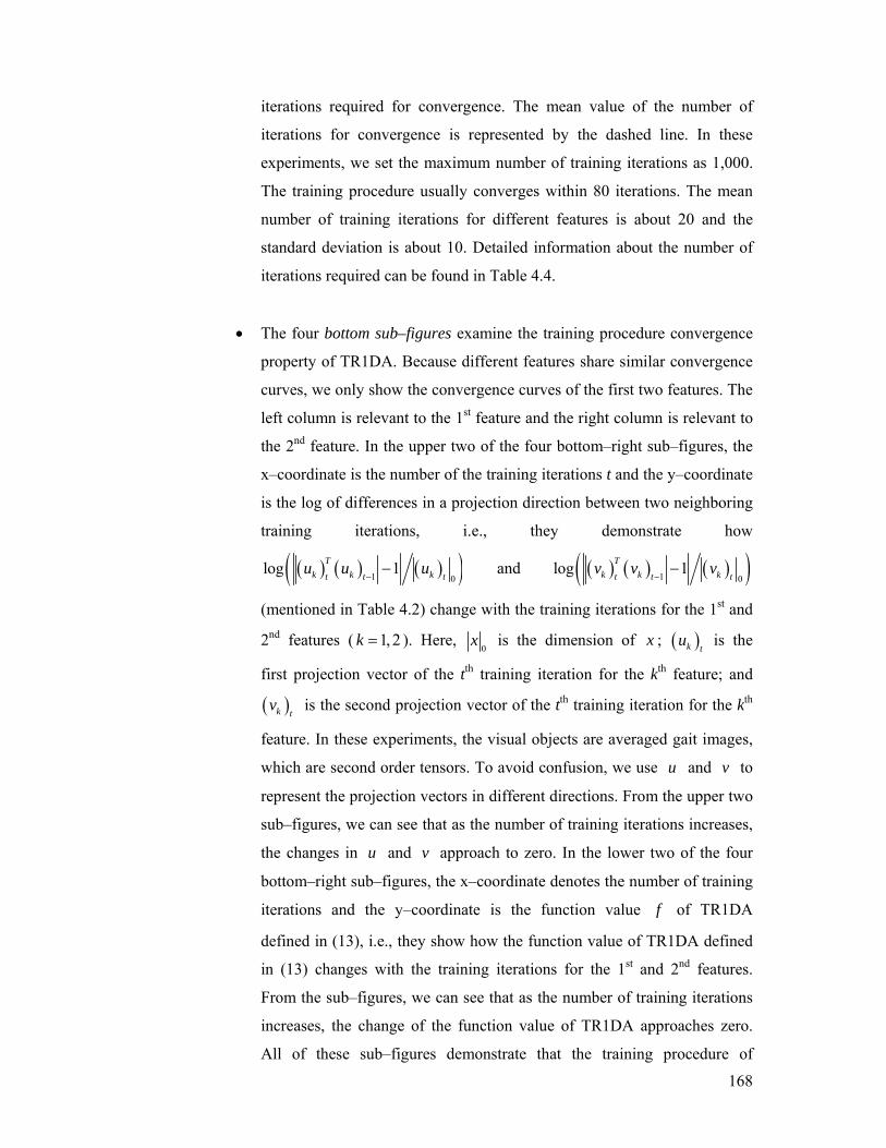
168
iterations required for convergence. The mean value of the number of
iterations for convergence is represented by the dashed line. In these
experiments, we set the maximum number of training iterations as 1,000.
The training procedure usually converges within 80 iterations. The mean
number of training iterations for different features is about 20 and the
standard deviation is about 10. Detailed information about the number of
iterations required can be found in Table 4.4.
• The four bottom sub–figures examine the training procedure convergence
property of TR1DA. Because different features share similar convergence
curves, we only show the convergence curves of the first two features. The
left column is relevant to the 1st feature and the right column is relevant to
the 2nd feature. In the upper two of the four bottom–right sub–figures, the
x–coordinate is the number of the training iterations t and the y–coordinate
is the log of differences in a projection direction between two neighboring
training iterations, i.e., they demonstrate how
( ) ( ) ( )( )1 0log 1T
k k kt t tu u u
−− and ( ) ( ) ( )( )1 0
log 1Tk k kt t t
v v v−−
(mentioned in Table 4.2) change with the training iterations for the 1st and
2nd features ( 1,2k = ). Here, 0
x is the dimension of x ; ( )k tu is the
first projection vector of the tth training iteration for the kth feature; and
( )k tv is the second projection vector of the tth training iteration for the kth
feature. In these experiments, the visual objects are averaged gait images,
which are second order tensors. To avoid confusion, we use u and v to
represent the projection vectors in different directions. From the upper two
sub–figures, we can see that as the number of training iterations increases,
the changes in u and v approach to zero. In the lower two of the four
bottom–right sub–figures, the x–coordinate denotes the number of training
iterations and the y–coordinate is the function value f of TR1DA
defined in (13), i.e., they show how the function value of TR1DA defined
in (13) changes with the training iterations for the 1st and 2nd features.
From the sub–figures, we can see that as the number of training iterations
increases, the change of the function value of TR1DA approaches zero.
All of these sub–figures demonstrate that the training procedure of
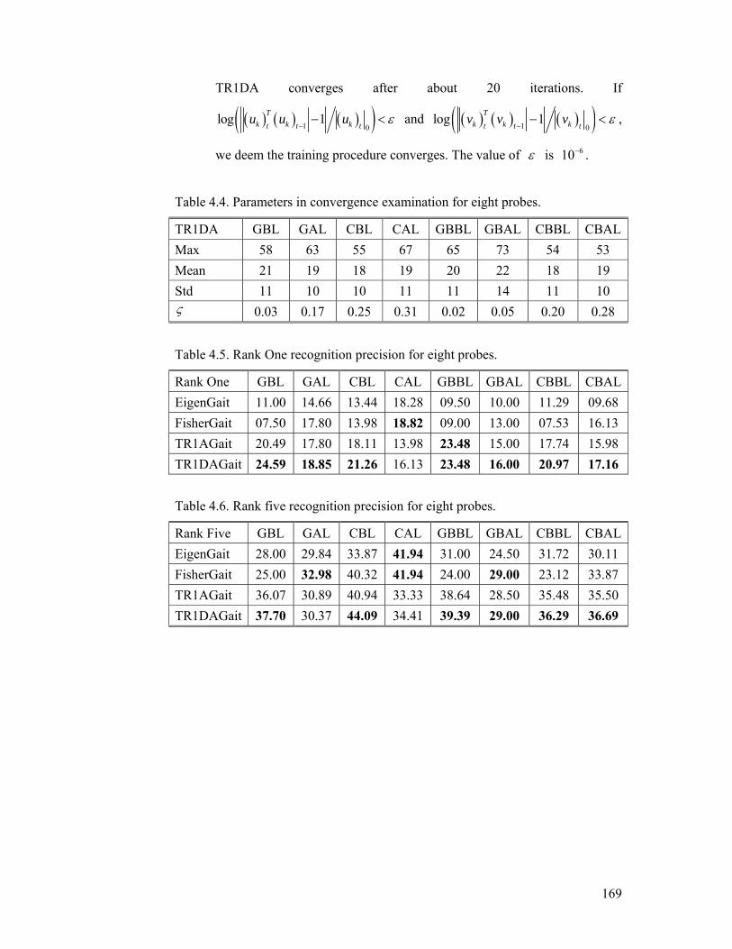
169
TR1DA converges after about 20 iterations. If
( ) ( ) ( )( )1 0log 1T
k k kt t tu u u ε
−− < and ( ) ( ) ( )( )1 0
log 1Tk k kt t t
v v v ε−− < ,
we deem the training procedure converges. The value of ε is 610− .
Table 4.4. Parameters in convergence examination for eight probes.
TR1DA GBL GAL CBL CAL GBBL GBAL CBBL CBALMax 58 63 55 67 65 73 54 53 Mean 21 19 18 19 20 22 18 19 Std 11 10 10 11 11 14 11 10 ς 0.03 0.17 0.25 0.31 0.02 0.05 0.20 0.28
Table 4.5. Rank One recognition precision for eight probes.
Rank One GBL GAL CBL CAL GBBL GBAL CBBL CBALEigenGait 11.00 14.66 13.44 18.28 09.50 10.00 11.29 09.68 FisherGait 07.50 17.80 13.98 18.82 09.00 13.00 07.53 16.13 TR1AGait 20.49 17.80 18.11 13.98 23.48 15.00 17.74 15.98 TR1DAGait 24.59 18.85 21.26 16.13 23.48 16.00 20.97 17.16
Table 4.6. Rank five recognition precision for eight probes.
Rank Five GBL GAL CBL CAL GBBL GBAL CBBL CBALEigenGait 28.00 29.84 33.87 41.94 31.00 24.50 31.72 30.11 FisherGait 25.00 32.98 40.32 41.94 24.00 29.00 23.12 33.87 TR1AGait 36.07 30.89 40.94 33.33 38.64 28.50 35.48 35.50 TR1DAGait 37.70 30.37 44.09 34.41 39.39 29.00 36.29 36.69
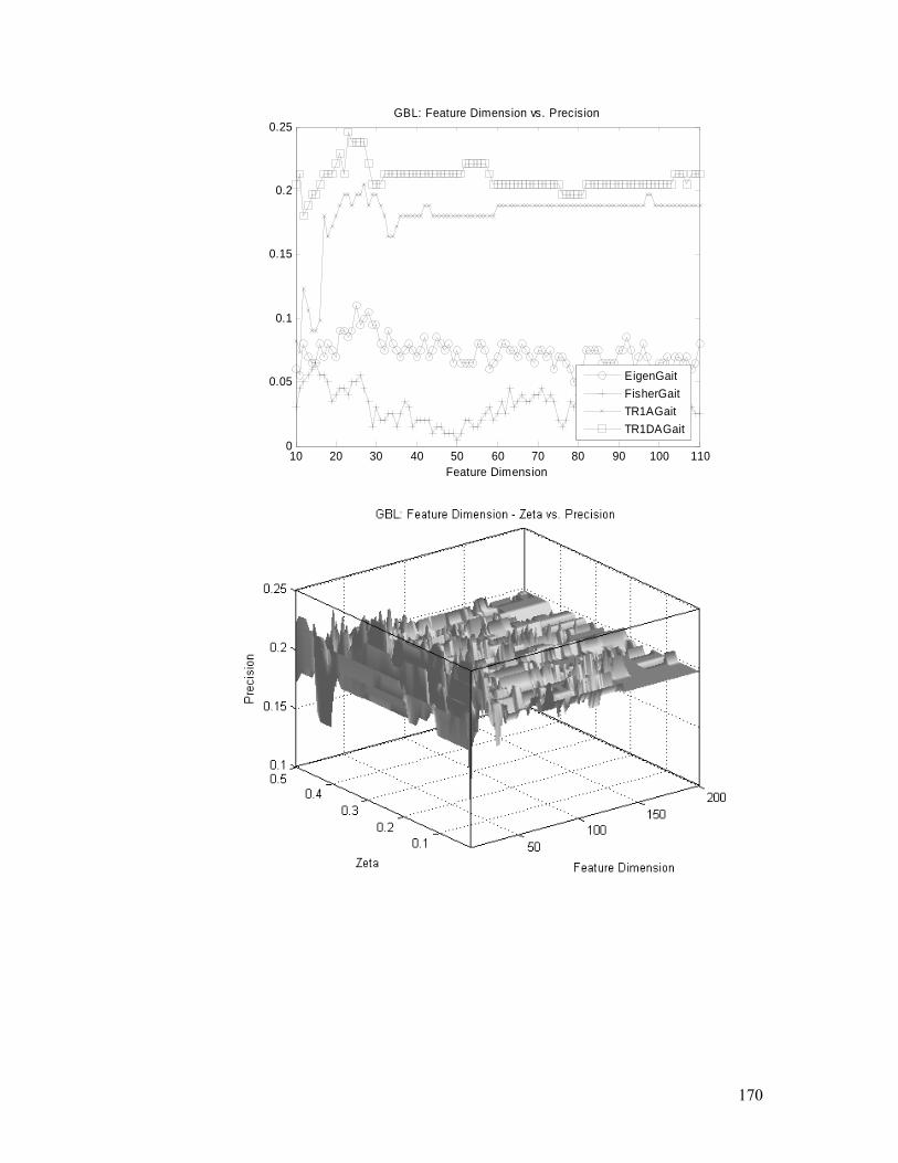
170
10 20 30 40 50 60 70 80 90 100 1100
0.05
0.1
0.15
0.2
0.25
Feature Dimension
GBL: Feature Dimension vs. Precision
EigenGaitFisherGaitTR1AGaitTR1DAGait
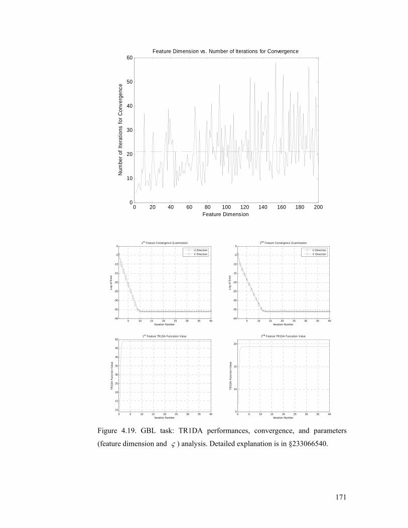
171
0 20 40 60 80 100 120 140 160 180 2000
10
20
30
40
50
60Feature Dimension vs. Number of Iterations for Convergence
Feature Dimension
Num
ber o
f Ite
ratio
ns fo
r Con
verg
ence
5 10 15 20 25 30 35 40-40
-35
-30
-25
-20
-15
-10
-5
01st Feature Convergence Examination
Iteration Number
Log
of E
rror
U DirectionV Direction
5 10 15 20 25 30 35 40-40
-35
-30
-25
-20
-15
-10
-5
02nd Feature Convergence Examination
Iteration Number
Log
of E
rror
U DirectionV Direction
0 5 10 15 20 25 30 35 4010
15
20
25
30
35
40
45
501st Feature TR1DA Funcation Value
Iteration Number
TR1D
A F
unct
ion
Val
ue
0 5 10 15 20 25 30 35 405
10
15
20
2nd Feature TR1DA Funcation Value
Iteration Number
TR1D
A F
unct
ion
Val
ue
Figure 4.19. GBL task: TR1DA performances, convergence, and parameters
(feature dimension and ς ) analysis. Detailed explanation is in §233066540.
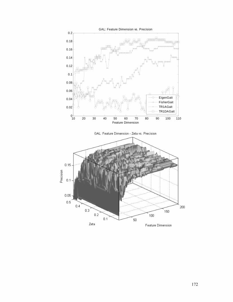
172
10 20 30 40 50 60 70 80 90 100 1100
0.02
0.04
0.06
0.08
0.1
0.12
0.14
0.16
0.18
0.2
Feature Dimension
GAL: Feature Dimension vs. Precision
EigenGaitFisherGaitTR1AGaitTR1DAGait
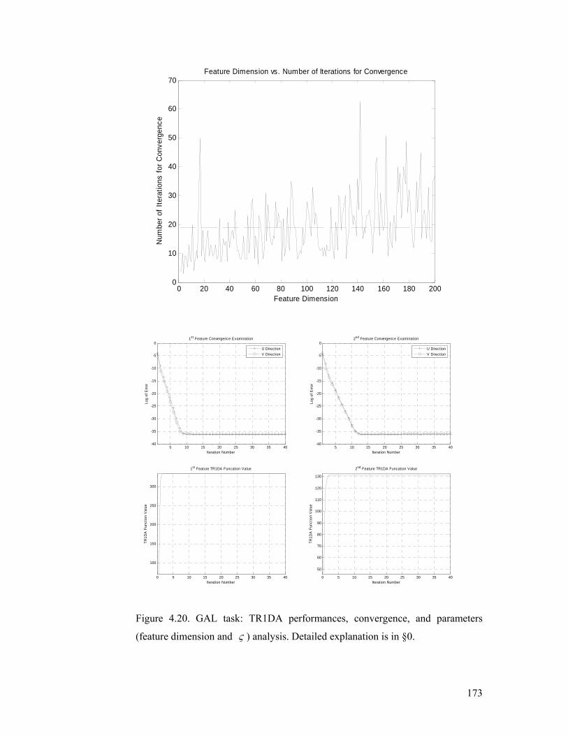
173
0 20 40 60 80 100 120 140 160 180 2000
10
20
30
40
50
60
70Feature Dimension vs. Number of Iterations for Convergence
Feature Dimension
Num
ber o
f Ite
ratio
ns fo
r Con
verg
ence
5 10 15 20 25 30 35 40-40
-35
-30
-25
-20
-15
-10
-5
01st Feature Convergence Examination
Iteration Number
Log
of E
rror
U DirectionV Direction
5 10 15 20 25 30 35 40-40
-35
-30
-25
-20
-15
-10
-5
02nd Feature Convergence Examination
Iteration Number
Log
of E
rror
U DirectionV Direction
0 5 10 15 20 25 30 35 40
100
150
200
250
300
1st Feature TR1DA Funcation Value
Iteration Number
TR1D
A F
unct
ion
Val
ue
0 5 10 15 20 25 30 35 40
50
60
70
80
90
100
110
120
130
2nd Feature TR1DA Funcation Value
Iteration Number
TR1D
A F
unct
ion
Val
ue
Figure 4.20. GAL task: TR1DA performances, convergence, and parameters
(feature dimension and ς ) analysis. Detailed explanation is in §0.
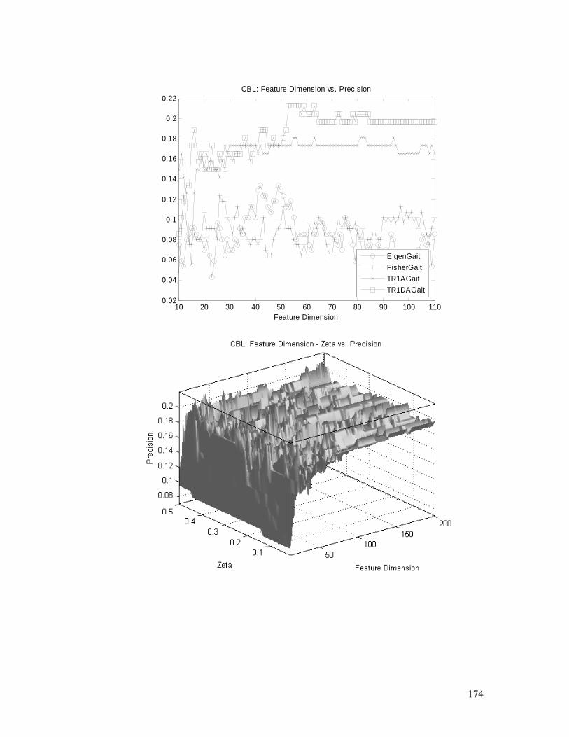
174
10 20 30 40 50 60 70 80 90 100 1100.02
0.04
0.06
0.08
0.1
0.12
0.14
0.16
0.18
0.2
0.22
Feature Dimension
CBL: Feature Dimension vs. Precision
EigenGaitFisherGaitTR1AGaitTR1DAGait
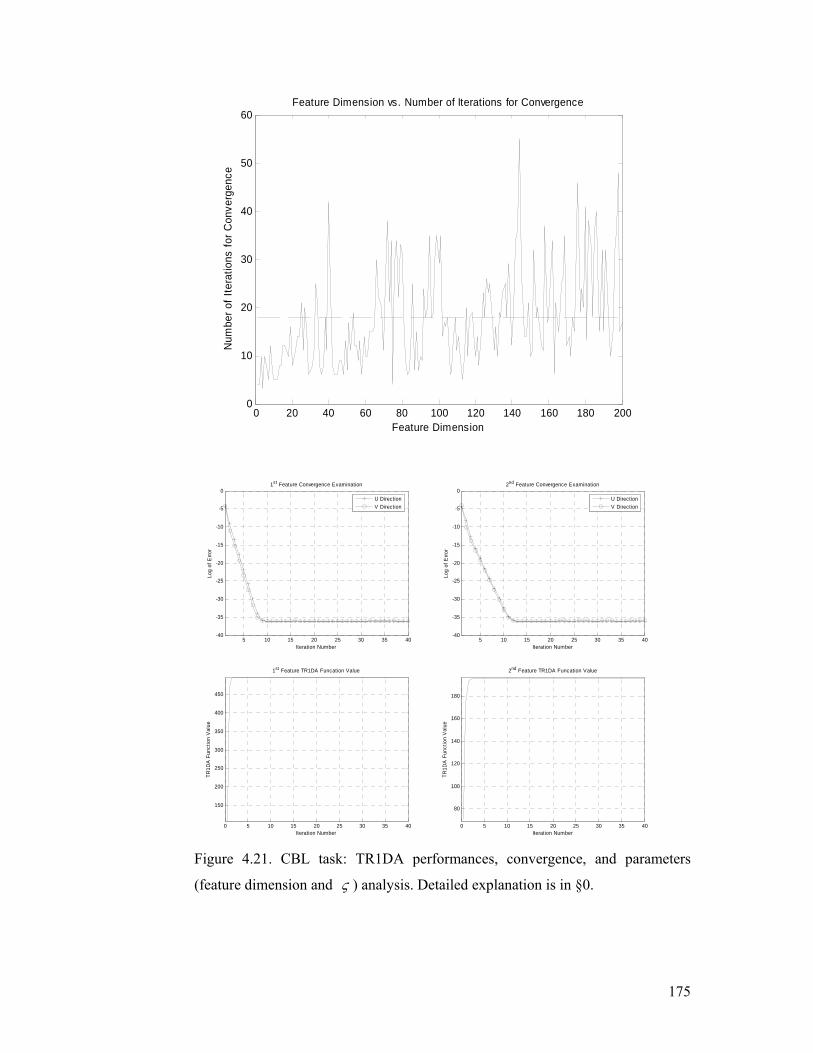
175
0 20 40 60 80 100 120 140 160 180 2000
10
20
30
40
50
60Feature Dimension vs. Number of Iterations for Convergence
Feature Dimension
Num
ber o
f Ite
ratio
ns fo
r Con
verg
ence
5 10 15 20 25 30 35 40-40
-35
-30
-25
-20
-15
-10
-5
01st Feature Convergence Examination
Iteration Number
Log
of E
rror
U DirectionV Direction
5 10 15 20 25 30 35 40-40
-35
-30
-25
-20
-15
-10
-5
02nd Feature Convergence Examination
Iteration Number
Log
of E
rror
U DirectionV Direction
0 5 10 15 20 25 30 35 40
150
200
250
300
350
400
450
1st Feature TR1DA Funcation Value
Iteration Number
TR1D
A F
unct
ion
Val
ue
0 5 10 15 20 25 30 35 40
80
100
120
140
160
180
2nd Feature TR1DA Funcation Value
Iteration Number
TR1D
A F
unct
ion
Val
ue
Figure 4.21. CBL task: TR1DA performances, convergence, and parameters
(feature dimension and ς ) analysis. Detailed explanation is in §0.
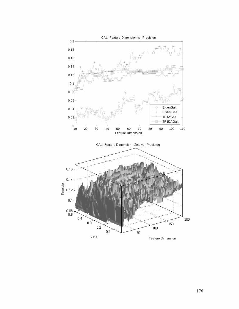
176
10 20 30 40 50 60 70 80 90 100 1100
0.02
0.04
0.06
0.08
0.1
0.12
0.14
0.16
0.18
0.2
Feature Dimension
CAL: Feature Dimension vs. Precision
EigenGaitFisherGaitTR1AGaitTR1DAGait

177
0 20 40 60 80 100 120 140 160 180 2000
10
20
30
40
50
60
70Feature Dimension vs. Number of Iterations for Convergence
Feature Dimension
Num
ber o
f Ite
ratio
ns fo
r Con
verg
ence
5 10 15 20 25 30 35 40-40
-35
-30
-25
-20
-15
-10
-5
01st Feature Convergence Examination
Iteration Number
Log
of E
rror
U DirectionV Direction
5 10 15 20 25 30 35 40-40
-35
-30
-25
-20
-15
-10
-5
02nd Feature Convergence Examination
Iteration Number
Log
of E
rror
U DirectionV Direction
0 5 10 15 20 25 30 35 40
150
200
250
300
350
400
450
500
550
600
1st Feature TR1DA Funcation Value
Iteration Number
TR1D
A F
unct
ion
Val
ue
0 5 10 15 20 25 30 35 40
100
120
140
160
180
200
220
240
2nd Feature TR1DA Funcation Value
Iteration Number
TR1D
A F
unct
ion
Val
ue
Figure 4.22. CAL task: TR1DA performances, convergence, and parameters
(feature dimension and ς ) analysis. Detailed explanation is in §0.
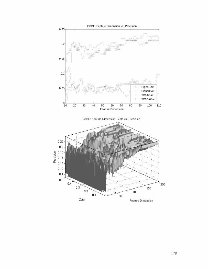
178
10 20 30 40 50 60 70 80 90 100 1100
0.05
0.1
0.15
0.2
0.25
Feature Dimension
GBBL: Feature Dimension vs. Precision
EigenGaitFisherGaitTR1AGaitTR1DAGait
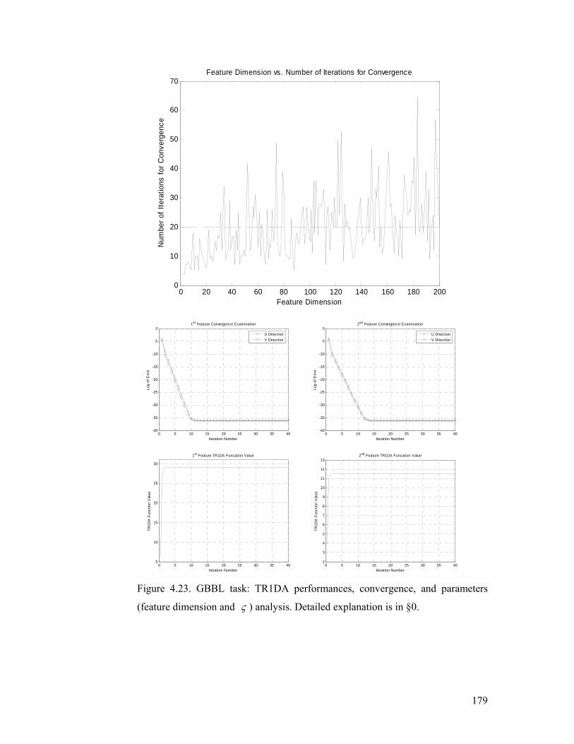
179
0 20 40 60 80 100 120 140 160 180 2000
10
20
30
40
50
60
70Feature Dimension vs. Number of Iterations for Convergence
Feature Dimension
Num
ber o
f Ite
ratio
ns fo
r Con
verg
ence
0 5 10 15 20 25 30 35 40-40
-35
-30
-25
-20
-15
-10
-5
01st Feature Convergence Examination
Iteration Number
Log
of E
rror
U DirectionV Direction
0 5 10 15 20 25 30 35 40-40
-35
-30
-25
-20
-15
-10
-5
02nd Feature Convergence Examination
Iteration Number
Log
of E
rror
U DirectionV Direction
0 5 10 15 20 25 30 35 405
10
15
20
25
30
1st Feature TR1DA Funcation Value
Iteration Number
TR1D
A F
unct
ion
Val
ue
0 5 10 15 20 25 30 35 402
3
4
5
6
7
8
9
10
11
12
132nd Feature TR1DA Funcation Value
Iteration Number
TR1D
A F
unct
ion
Val
ue
Figure 4.23. GBBL task: TR1DA performances, convergence, and parameters
(feature dimension and ς ) analysis. Detailed explanation is in §0.
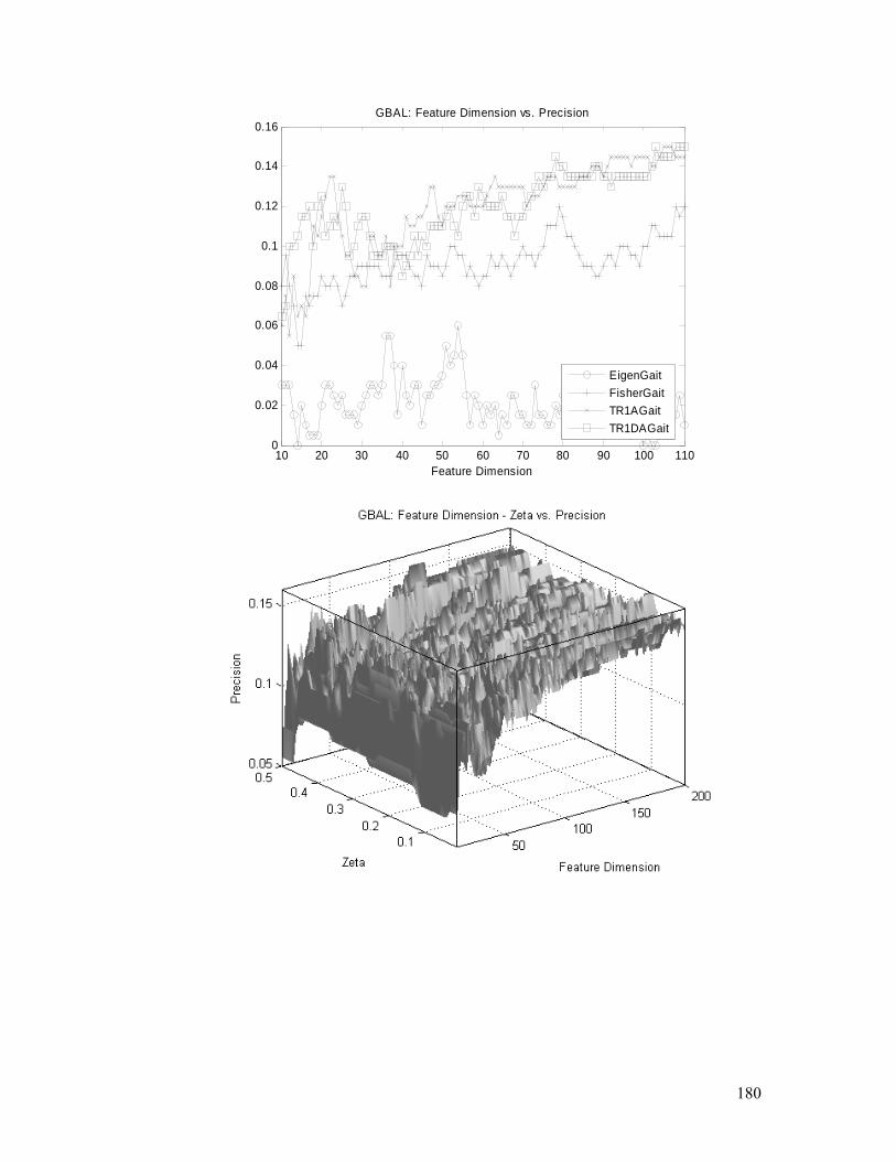
180
10 20 30 40 50 60 70 80 90 100 1100
0.02
0.04
0.06
0.08
0.1
0.12
0.14
0.16
Feature Dimension
GBAL: Feature Dimension vs. Precision
EigenGaitFisherGaitTR1AGaitTR1DAGait
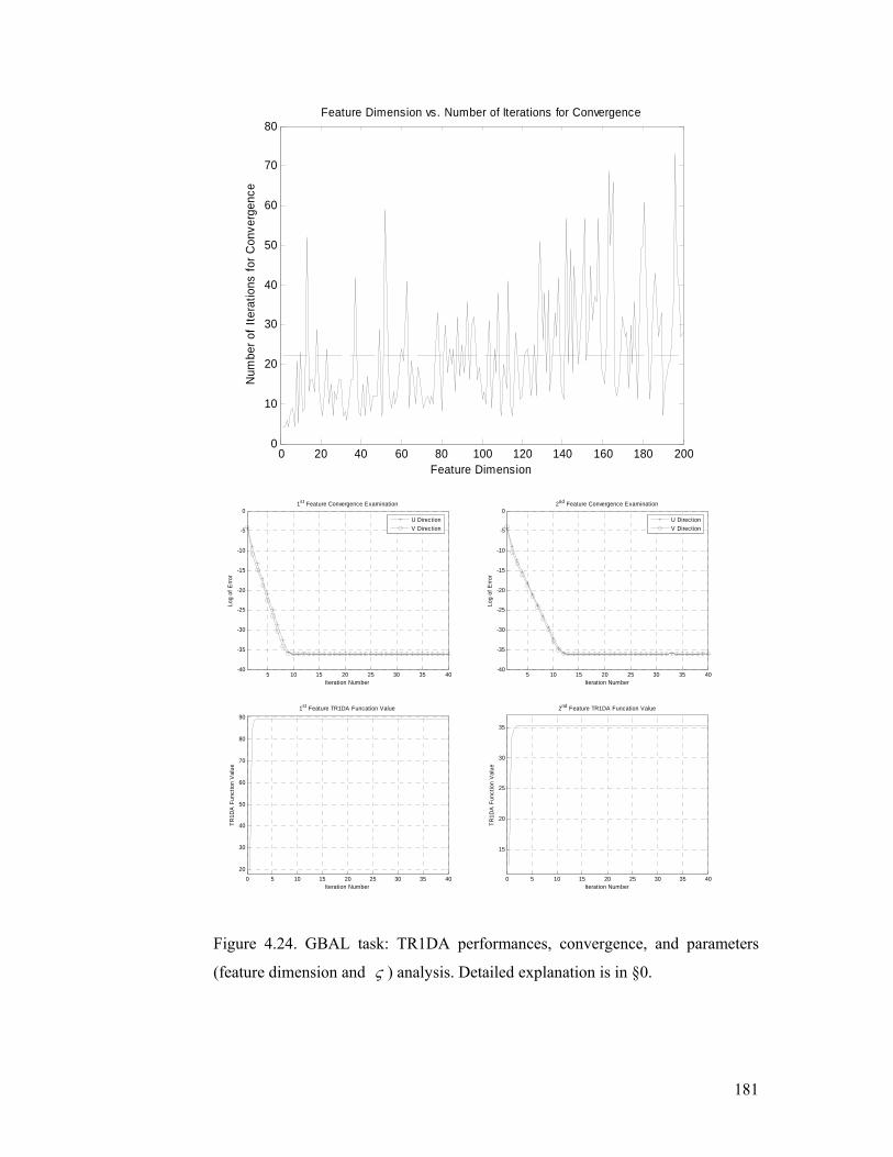
181
0 20 40 60 80 100 120 140 160 180 2000
10
20
30
40
50
60
70
80Feature Dimension vs. Number of Iterations for Convergence
Feature Dimension
Num
ber o
f Ite
ratio
ns fo
r Con
verg
ence
5 10 15 20 25 30 35 40-40
-35
-30
-25
-20
-15
-10
-5
01st Feature Convergence Examination
Iteration Number
Log
of E
rror
U DirectionV Direction
5 10 15 20 25 30 35 40-40
-35
-30
-25
-20
-15
-10
-5
02nd Feature Convergence Examination
Iteration Number
Log
of E
rror
U DirectionV Direction
0 5 10 15 20 25 30 35 4020
30
40
50
60
70
80
901st Feature TR1DA Funcation Value
Iteration Number
TR1D
A F
unct
ion
Val
ue
0 5 10 15 20 25 30 35 40
15
20
25
30
35
2nd Feature TR1DA Funcation Value
Iteration Number
TR1D
A F
unct
ion
Val
ue
Figure 4.24. GBAL task: TR1DA performances, convergence, and parameters
(feature dimension and ς ) analysis. Detailed explanation is in §0.
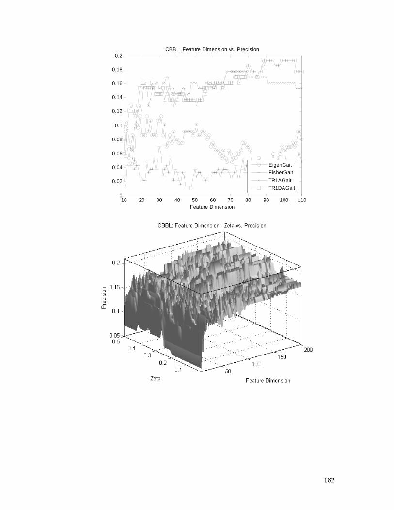
182
10 20 30 40 50 60 70 80 90 100 1100
0.02
0.04
0.06
0.08
0.1
0.12
0.14
0.16
0.18
0.2
Feature Dimension
CBBL: Feature Dimension vs. Precision
EigenGaitFisherGaitTR1AGaitTR1DAGait
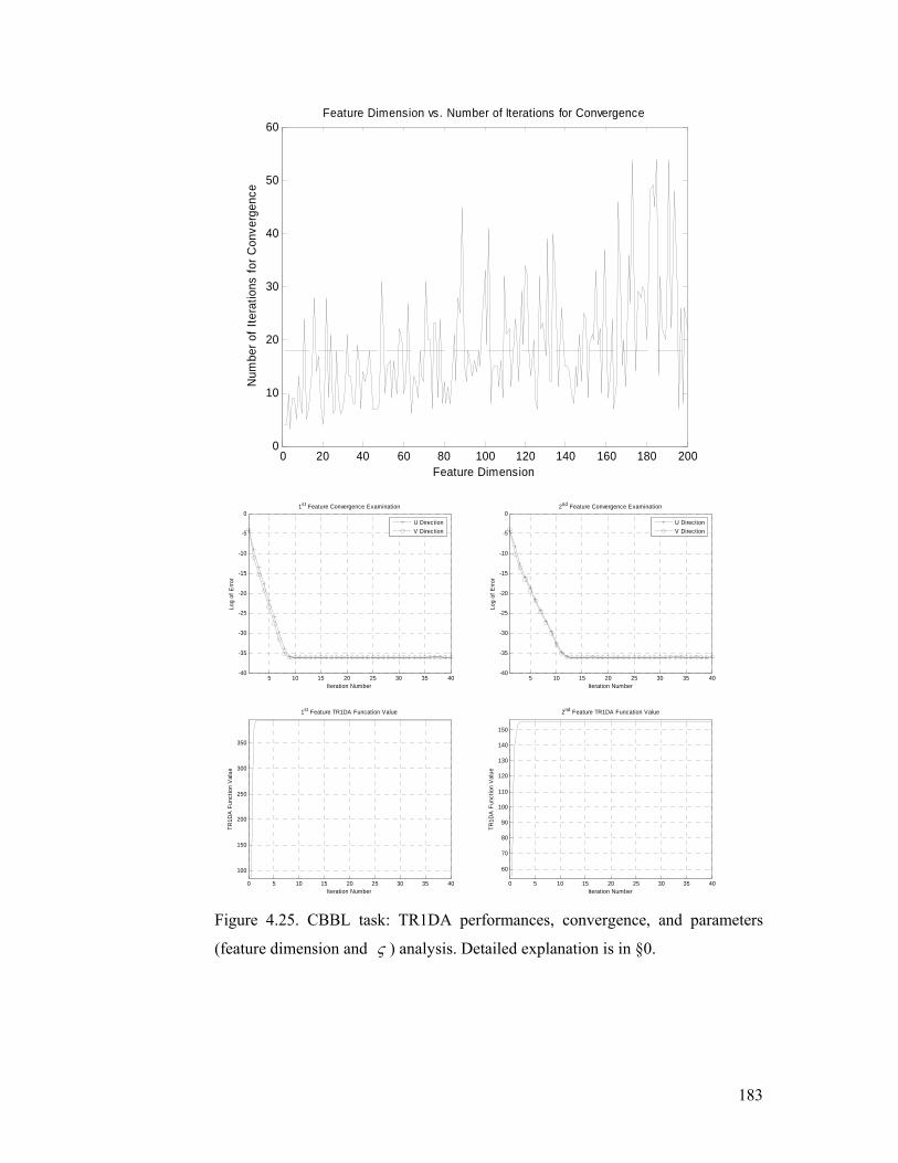
183
0 20 40 60 80 100 120 140 160 180 2000
10
20
30
40
50
60Feature Dimension vs. Number of Iterations for Convergence
Feature Dimension
Num
ber o
f Ite
ratio
ns fo
r Con
verg
ence
5 10 15 20 25 30 35 40-40
-35
-30
-25
-20
-15
-10
-5
01st Feature Convergence Examination
Iteration Number
Log
of E
rror
U DirectionV Direction
5 10 15 20 25 30 35 40-40
-35
-30
-25
-20
-15
-10
-5
02nd Feature Convergence Examination
Iteration Number
Log
of E
rror
U DirectionV Direction
0 5 10 15 20 25 30 35 40
100
150
200
250
300
350
1st Feature TR1DA Funcation Value
Iteration Number
TR1D
A F
unct
ion
Val
ue
0 5 10 15 20 25 30 35 40
60
70
80
90
100
110
120
130
140
150
2nd Feature TR1DA Funcation Value
Iteration Number
TR1D
A F
unct
ion
Val
ue
Figure 4.25. CBBL task: TR1DA performances, convergence, and parameters
(feature dimension and ς ) analysis. Detailed explanation is in §0.
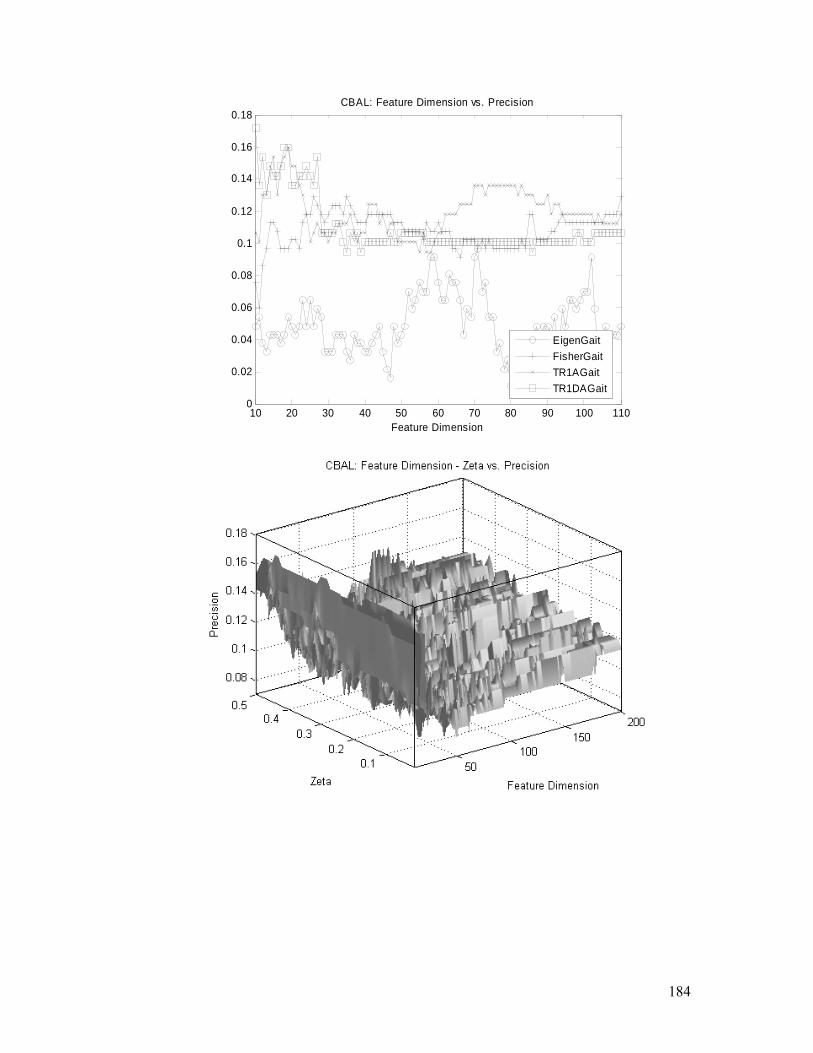
184
10 20 30 40 50 60 70 80 90 100 1100
0.02
0.04
0.06
0.08
0.1
0.12
0.14
0.16
0.18
Feature Dimension
CBAL: Feature Dimension vs. Precision
EigenGaitFisherGaitTR1AGaitTR1DAGait
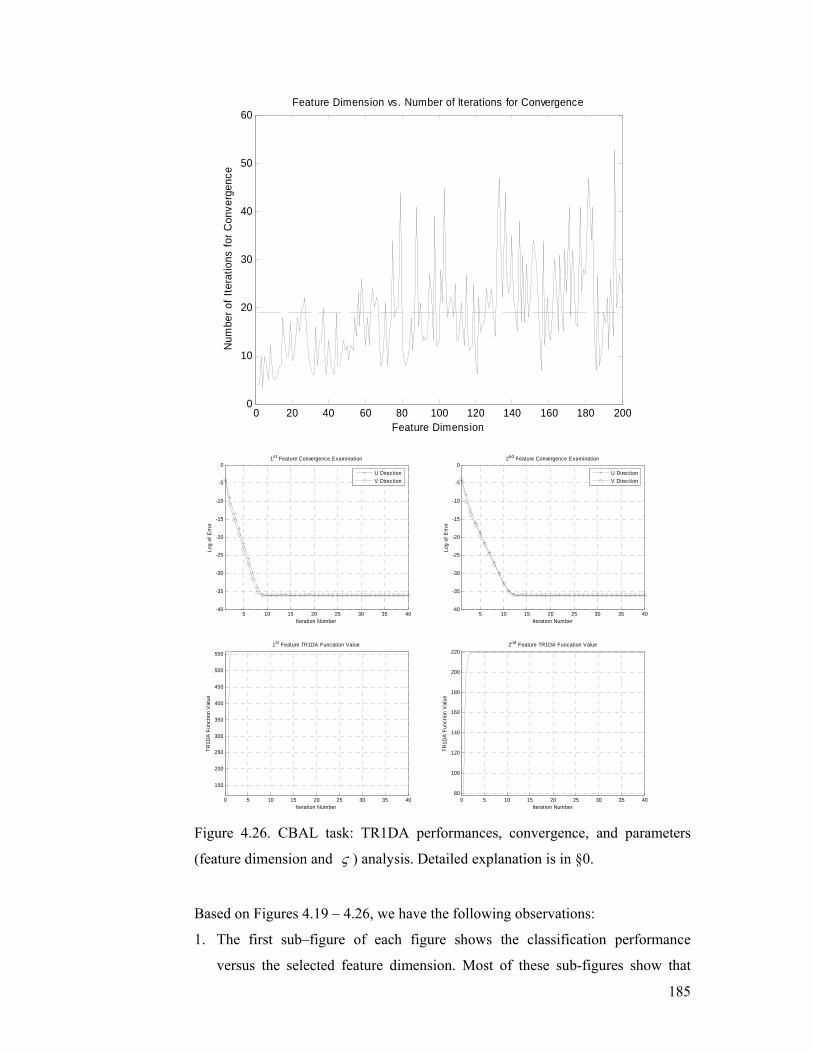
185
0 20 40 60 80 100 120 140 160 180 2000
10
20
30
40
50
60Feature Dimension vs. Number of Iterations for Convergence
Feature Dimension
Num
ber o
f Ite
ratio
ns fo
r Con
verg
ence
5 10 15 20 25 30 35 40-40
-35
-30
-25
-20
-15
-10
-5
01st Feature Convergence Examination
Iteration Number
Log
of E
rror
U DirectionV Direction
5 10 15 20 25 30 35 40-40
-35
-30
-25
-20
-15
-10
-5
02nd Feature Convergence Examination
Iteration Number
Log
of E
rror
U DirectionV Direction
0 5 10 15 20 25 30 35 40
150
200
250
300
350
400
450
500
550
1st Feature TR1DA Funcation Value
Iteration Number
TR1D
A F
unct
ion
Val
ue
0 5 10 15 20 25 30 35 4080
100
120
140
160
180
200
2202nd Feature TR1DA Funcation Value
Iteration Number
TR1D
A F
unct
ion
Val
ue
Figure 4.26. CBAL task: TR1DA performances, convergence, and parameters
(feature dimension and ς ) analysis. Detailed explanation is in §0.
Based on Figures 4.19 – 4.26, we have the following observations:
1. The first sub–figure of each figure shows the classification performance
versus the selected feature dimension. Most of these sub-figures show that
186
tensor based subspace selection methods (TR1DA and TR1A) perform better
than vector based ones (LDA and PCA) and the discriminative subspace
selection methods (TR1DA and LDA) perform better than reconstructive
subspace selection methods (TR1A and PCA). This is because the size of the
gallery, i.e., the training set, in different tasks is much less than the dimension
of original features, i.e., the appearance of the averaged gait image for
representation. According to the discussions at the beginning of this Chapter,
we know tensor based subspace selection methods reduce the over fitting
problem when training samples are limited, so TR1DA and TR1A should
perform better than LDA and PCA, respectively. Moreover, tasks here are
classification so discriminative based methods perform better than
reconstructive based methods as discussed at the beginning of Chapter 2;
2. The second sub–figure of each figure shows the classification performance of
TR1DA versus the parameters in TR1DA. There are two parameters for
TR1DA, which are ς and selected feature dimension. Some of these sub-
figures show that the more the selected features are, the higher the
classification accuracy is for the first selected 200 features; and some of them
show that with the increasing number of selected features, the classification
accuracy is initially increasing and then decreasing. From a large number of
experiences in subspace selection, we know the latter is more reasonable than
the former, so we believe we can have the similar observations as the latter if
more features are selected for evaluation;
3. The third sub–figure of each figure shows the number of iterations required to
meet the training stage convergence condition in TR1DA for different
features. According to Table 4.4, normally, TR1DA needs about 20 iterations
to converge and the corresponding standard deviation is about 10. Therefore,
for most features, we need about 30 iterations for training. The distributions of
the number of training iterations are similar to noise, i.e., there is no clear
relationship between the number of training iterations and the selected
features. This is because the training processes for different features are
independent, as shown in Section 4.4; and
4. The last four sub–figures of each figure demonstrate the convergence property
of the training stage of TR1DA. The first two sub–figures show that the
difference between the projection vectors of two consecutive training

187
iterations is decreasing with the increasing number of the training iterations;
and the last two sub–figures show the TR1DA function value is increasing
with the increasing number of the training iterations. These two points consist
with the mathematical proof of the theorem 4.1.
188
Summary
In this Chapter, the vector based learning is extended to accept tensors as input.
The result is a supervised tensor learning (STL) framework, which is the
multilinear extension of convex optimization based learning. To obtain the
solution of an STL based learning algorithm, the alternating projection method is
used. Based on STL and its alternating projection optimization algorithm, we
illustrate several examples. That is we extend the soft margin support vector
machine (SVM), the nu–SVM, the least squares SVM, the minimax probability
machine (MPM), the Fisher discriminant analysis (FDA), the distance metric
learning (DML) to their tensor versions, which are the soft margin support tensor
machine (STM), the nu–STM, the least squares STM, the tensor MPM (TMPM),
the tensor FDA (TFDA), and the multiple distance metrices learning (MDML).
Based on STL, we also introduce a method for iterative feature extraction: the
iterative feature extraction model (IFEM). As an example, we develop the tensor
rank one discriminant analysis (TR1DA).
Finally, we implement TMPM for image classification and TR1DA for the
elapsed time problem in human gait recognition. By comparing TMPM with
MPM, we show that TMPM reduces the overfitting problem in MPM. By
comparing TR1DA with principal component analysis (PCA), linear discriminant
analysis (LDA), and tensor rank one analysis (TR1A), we show that TR1DA
reduces the small sample size problem and always achieves the best performance
on the elapsed time problem in human gait recognition.
189
5. Thesis Conclusion
Linear discriminant analysis (LDA) motivates this thesis. This is because LDA
has many problems, although it has been deemed as one of the most important
linear subspace methods in pattern classification and it has been widely applied in
many applications, e.g., face recognition [34][168], image retrieval [139][152]
[153][154], video data organization [43], gait recognition [46], speech recognition
[67][70], document classification [108], music management [85], network flow
analysis [136], and video surveillance [143][144].
The first type of the problems with LDA is model based: 1) the heteroscedastic
problem [29][28][70][61][99], 2) the multimodal problem [51][28], and 3) the
class separation problem [103][95][96][99][146]. To deal with the model based
problems, we begin with the fact that LDA selects the subspace to maximize the
arithmetic mean of the Kullback–Leibler (KL) [21] divergences between different
classes, when samples are sampled from Gaussian distributions [60] with identical
covariances. We then generalize LDA in two ways: 1) extending the KL
divergence to the Bregman divergence [14]; and 2) extending the arithmetic mean
to the generalized mean [48]. The result of these generalizations is the general
averaged divergences analysis and the significance of the generalization is a
discriminative subspace selection framework, from which we can develope a
number of different methods to select discriminative features. Based on this
framework, we analyze the geometric based subspace selection: 1) the geometric
mean of divergences between different classes, 2) the geometric mean of
normalized divergences between different classes, and 3) the geometric mean of
all divergences (the divergences and the normalized divergences) between
different classes. The first method is studied because the geometric mean
increases the effects of small divergences and at the same time reduces the effects
of large divergences. The second method is studied to further reduce the effects of
large divergences. The intuition is the product of normalized divergences is large
when they are similar to each other. However, the second method cannot be
directly used for subspace selection. This is because there are subspaces in which
all divergences become small, but all normalized divergences are comparable in
size. Consequently, we linearly combine the first and the second methods
190
together. To apply the geometric mean based subspace selection for real
applications, we suppose the samples are sampled from Gaussian distributions and
we use the KL divergence to measure differences between different classes.
Because we drop the identical covariances assumption in LDA, we do not meet
the heteroscedastic problem. The advantages of the combination of the geometric
mean and the KL divergences are: 1) it is compatible with the heteroscedastic
property of the distributions of samples in different classes; 2) it selects suitable
discriminative subspace when samples are drawn from Gaussian mixture models;
and 3) it significantly reduces the class separation problem when KL divergences
of difffernt classes are not evenly distributed. For real applications, we use the
Gaussian mixture model to model the samples in each class, and thus avoid the
multimodal problem. Based on a large number of experiments, from synthetic
data to hand writing digital recognition, the geometric mean combined with the
KL divergence outperforms LDA and its representative extensions.
The second type of these problems with LDA is the small sample size (SSS)
problem [38][49][139][123][19][175][55][173][174][180]. LDA meets this
problem when the number of training samples is less than the dimension of the
feature space. In computer vision research, this problem can be reduced in a
natural way by introducing the structure information as constraints, because
objects in computer vision research are always represented by multidimensional
arrays, i.e., tensors [75]. For example, a face image in face recognition, an
averaged gait image in human gait recognition, and a video shot in video
management. Although there are some algorithms applying the structure
information for subspace selection, e.g., tensor rank one analysis (TR1A) [132],
general tensor analysis (GTA) [75][162][171], and two dimensional linear
discriminant analysis (2DLDA) [174], each of these methods has its own
drawbacks for classification. TR1A and GTA are reconstructive models, i.e., they
are used to produce representations for sufficient reconstruction but not for
classification. The 2DLDA fails to converge in the training stage, although its
effectiveness and efficiency have been demonstrated through face recognition
applications. Here, we propose a different discriminative multilinear subspace
method, the general tensor discriminant analysis (GTDA) [144][147], by
combining the differential scatter discriminant criterion and the operations in
multilinear algebra [115][75]. Compared with TR1A, GTA, and 2DLDA, GTDA
191
has the following benefits: 1) provision with a converged alternating projection
training algorithm to obtain a solution, while 2DLDA does not; 2) preservation of
more discriminative information of training samples; 3) acceptance of general
tensors as input; and 4) reduction of the SSS problem in the subsequent
classification, e.g., by LDA. We further extend GTDA by combining the manifold
learning [13] and the operations in multilinear algebra to make the manifold
learning algorithms accept general tensors as input. To examine the effictiveness
and the efficiency of GTDA, we apply it for human gait recognition. Based on a
great deal of comparison, GTDA combined with LDA always achieves the top
level performance for USF HumanID gait database [126].
In supervised learning [30][39], when the size of training samples is small,
learning machines encounter the overfitting problem. Similar to the motivation in
GTDA, we also utilize the structure information as constraints to reduce the
overfitting problem by decreasing the number of parameters needed to model the
training samples. This results in a supervised tensor learning (STL) [149][150]
framework. The framework extends the convex optimization [11] based learning
to accept general tensors as input. To obtain the solution of the algorithms under
the STL framework, we develop an alternating projection method. Based on STL
and its alternating projection optimization algorithm, we illustrate the following
examples, which are the support tensor machine (STM), the tensor minimax
probability machine (TMPM), the tensor Fisher discriminant analysis (TFDA), the
multiple distance metrics learning (MDML). Motivated by TR1A and based on
STL, we develop the tensor rank one discriminant analysis (TR1DA), which is an
iterative discriminative feature extraction method. Finally, we implement TMPM
and TR1DA for image classification and the elapsed time problem in human gait
recognition, respectively. By comparing TMPM with MPM, we know TMPM
reduces the overfitting problem in supervised learning. By comparing TR1DA
with principal component analysis (PCA), linear discriminant analysis (LDA), and
tensor rank one analysis (TR1A), we know TR1DA reduces the SSS problem.
In summary, this thesis deals with non trivial problems in discriminative subspace
selection, which are how to select the most discriminative subspace for
classification and how to deal with the SSS problem or over-fitting problem. The
primary contributions of the thesis are as follows:
192
1) we develop a general averaged divergences analysis framework, which is
a combination of the generalized mean function and the Bregman
divergence, for discriminative subspace selection;
2) under this framework, a new method, which combines the geometric
mean and the Kullback–Leibler divergence, is developed to significantly
reduce the class separation problem. With theoretical analysis, we know
the method also reduces the heteroscedastic problem and the multimodal
problem;
3) the kernelization of this new method is also developed for nonlinear
problems. Unlike existing kernel algorithms, we prove the kernel version
is equivalent to the linear version followed by the kernel principal
component analysis;
4) a large number of empirical studies based on both synthetic and real data
show the new discriminative subspace selection method performs better
than LDA and its representative extensions;
5) we propose GTDA to reduce the SSS problem for LDA. The advantages
of GTDA compared with existing pre-processing methods, e.g., principal
component analysis (PCA), tensor rank one analysis (TR1A), general
tensor analysis (GTA), and two dimensional LDA (2DLDA), are: i)
reduction of the SSS problem for subsequent classification, e.g., by LDA,
ii) preservation of discriminative information in training tensors, while
PCA, TR1A, and MSA do not guarantee this, iii) provision with stable
recognition rates because the optimization algorithm of GTDA converges,
while that of 2DLDA does not, and iv) acceptance of general tensors as
input, while 2DLDA only accepts matrices as input;
6) we provide a mathematical proof to demonstrate the convergence property
at the training stage. The significance of the proof is it is the first
theoretical study for the convergence issue of the alternating projection
based training algorithms for tensor subspace selection;
7) we apply the developed GTDA to human gait recognition. By applying
Gabor filters for averaged gait image representation, GTDA for subspace
selection, and LDA for classification, we achieve the stat-of-the-art
performance; and

193
8) we develop a STL framework and an alternating projection optimization
algorithm to reduce the over–fitting problem in convex optimization
based learning. Based on them, we propose STM, TMPM, TFDA, and
MDML. Compared with existing popular classifiers, e.g., SVM, MPM,
FDA, and DML, the advantages of their tensor extensions are: i)
generalizing better for the small size training set than vector based
classifiers, ii) converging well in the training stage compared with
existing tensor classifiers, e.g., 2DLDA, and iii) reducing training
computational complexities of vector based classifiers.
194
6. Appendices
Appendix for Chapter 2
Let Lix R∈r ( 1 i n≤ ≤ ) be a zero mean set of training samples, i.e.,
( ) 11 0n
iim n x
== =∑r r . Let ( ) 1
1 n Ti ii
S n x x=
= ∑ r r be the covariance matrix, and let
U be the linear transformation matrix in PCA. The Frobenius norm is denoted by
Fro⋅ . We have the following properties of PCA as defined in Section 2.1.
Property 2.1: PCA maximizes the variance in the projected subspace, i.e.,
( ) 2
1
1arg max tr arg maxn
T Ti FroU U i
U SU U xn =
= ∑ r .
Proof.
( )
( )1
2
1 1
1arg max tr arg max tr
1 1arg max tr arg max
nT T T
i iU U i
n nT T T
i i i FroU Ui i
U SU U x x Un
U x x U U xn n
=
= =
⎛ ⎞⎛ ⎞= ⎜ ⎟⎜ ⎟
⎝ ⎠⎝ ⎠
= =
∑
∑ ∑
r r
r r r
Therefore, PCA maximizes the variance in the projected subspace. ■
Property 2.3: PCA minimizes the reconstruction error, i.e.,
( ) 2
1
1arg max tr arg minn
T Ti i FroU U i
U SU x UU xn =
= −∑ r r .
Proof.
It is sufficient to prove 2 2
1 1
1 1arg max arg minn n
T Ti i iFro FroU Ui i
U x x UU xn n= =
= −∑ ∑r r r .
( ) ( )
( )
2
1
1
1
1arg min
1arg min
1arg min
nT
i i FroU i
n TT Ti i i i
U i
nT T T T T T T Ti i i i i i i i
U i
x UU xn
x UU x x UU xn
x x x UU x x UU x x UU UU xn
=
=
=
−
= − −
= − − +
∑
∑
∑
r r
r r r r
r r r r r r r r
In PCA, because TU U I= , we have
195
( )
( )
( )
1
1
1
2
1
1arg min
1arg min
1arg min
1arg max
nT T T T T T T Ti i i i i i i i
U i
nT T Ti i i i
U i
nT Ti i
U i
nT
i FroU i
x x x UU x x UU x x UU UU xn
x x x UU xn
x UU xn
U xn
=
=
=
=
− − +
= −
= −
=
∑
∑
∑
∑
r r r r r r r r
r r r r
r r
r
Therefore, PCA minimizes the reconstruction error. ■
Property 2.4: PCA decorrelates the training samples in the projected subspace.
Proof.
Let U be the projection, which is calculated according to PCA. Project all
training samples ixr using U as Ti iy U x=r r , where 'L LU R ×∈ .
Therefore, the covariance of the projected data is
( )( )1 1
1 1n n TT T Ty i i i i
i i
S y y U x U xn n= =
= =∑ ∑r r r r
1 1
1 1n nT T T T
i i i ii i
U x x U U x x Un n= =
⎛ ⎞= = ⎜ ⎟⎝ ⎠
∑ ∑r r r r
TU SU=
Because TU SU is a diagonal matrix, PCA decorrelates the training samples ixr
in the projected subspace. ■
Property 2.5: PCA maximizes the mutual information between xr and Ty U x=r r
on Gaussian data.
Proof.
Let U be the projection, which is calculated according to PCA. Project all
training samples xr using U as Ty U x=r r , where 'L LU R ×∈ .
The mutual information is ( ) ( ) ( )( ) ( )
,, , log
Y X
p x yI X Y p x y dXdY
p x p y= ∫ ∫
r rr r
r r and we
have ( ) ( ) ( ) ( ), |I X Y H Y H Y X H Y= − = , because Ty U x=r r . Here, ( )H Y is
the entropy of Y and ( )|H Y X is the entropy of Y with the given X .
196
The training samples are normally distributed with zero mean and covariance S ,
so the projected training samples are also normally distributed with zero mean and
covariance TyS U SU= . Therefore, the entropy ( )H yr is given by
( ) ( ) ( )logH y p y y dy= −∫r r r r
( )1 ' 1log 2 log2 2 2 y
N Sπ= + +
( )1 ' 1log 2 log2 2 2
TN U SUπ≤ + + .
Because U consists of the eigenvectors of S corresponding to the first largest
'L eigenvalues of S , U maximizes the mutual information on Gaussian data.
■
Observation 2.1: LDA maximizes the arithmetic mean of the KL divergences
between all pairs of classes, under the assumption that the Gaussian distributions
for different classes all have the same covariance matrix. The optimal projection
matrix U in LDA can be obtained by maximizing a particular ( )V Uϕ defined
in (2.38).
Proof.
According to (2.36) and (2.37), the KL divergence between the ith class and the jth
class in the projected subspace with the assumption of equal covariance matrices
( i jΣ = Σ = Σ ) is:
( ) ( )( )1|| tr constantT T
U i j ijD p p U U U D U−
= Σ + .
Then, we have
( )1
* arg max ||i j U i jU i j c
U q q D p p≤ ≠ ≤
= ∑
( )( )( )1
1 arg max tr T T
i j ijU i j c
q q U U U D U−
≤ ≠ ≤
= Σ∑
( ) 1
1
arg max tr T Ti j ij
U i j c
U U U q q D U−
≤ ≠ ≤
⎛ ⎞⎛ ⎞= Σ⎜ ⎟⎜ ⎟⎜ ⎟⎝ ⎠⎝ ⎠
∑
( )11
1 1
arg max trc c
T Ti j ij
U i j iU U U q q D U
−−
= = +
⎛ ⎞⎛ ⎞= Σ⎜ ⎟⎜ ⎟⎜ ⎟⎝ ⎠⎝ ⎠
∑ ∑ ,
where 1
ci i kk
q n n=
= ∑ is the prior probability of the ith class.
197
Because 1
1 1
c c
b i j iji j i
S q q D−
= = +
=∑ ∑ , as proved by Loog in [96], and t b wS S S= + = Σ
where bS , wS , and tS are defined in (2.10), we have:
( ) ( )( )1
1arg max || arg max tr T T
i j U i j w bU Ui j c
q q D p p U S U U S U−
≤ ≠ ≤
=∑ . ■
The generalized geometric mean is upper bounded by the arithmetic mean of the
divergences, i.e.,
( ) ( )111
1
|| ||i j
m nm n c
q qi jq q
U i j U i ji j ci j c m n
m n c
q qD p p D p p
q q≤ ≠ ≤≤ ≠ ≤≤ ≠ ≤
≤ ≠ ≤
⎛ ⎞⎜ ⎟∑⎡ ⎤ ≤⎣ ⎦ ⎜ ⎟⎜ ⎟⎝ ⎠
∑∏ ∑.
Proof.
Because 1
1
1i j
i j c m nm n c
q qq q≤ ≠ ≤
≤ ≠ ≤
=∑ ∑ and ( )|| 0U i jD p p > , according to the Jensen
inequality [21], we have
( )1
1
||i jU i j
i j c m nm n c
q qD p p
q q≤ ≠ ≤≤ ≠ ≤
∑ ∑
( )( )( )1
1
exp log ||i jU i j
i j c m nm n c
q qD p p
q q≤ ≠ ≤≤ ≠ ≤
= ∑ ∑
( )( )1
1
exp log ||i jU i j
i j c m nm n c
q qD p p
q q≤ ≠ ≤≤ ≠ ≤
⎛ ⎞⎜ ⎟≥ ⎜ ⎟⎜ ⎟⎝ ⎠∑ ∑
( ) 11
||i j
m nm n c
q q
q qU i j
i j c
D p p≤ ≠ ≤
≤ ≠ ≤
∑⎡ ⎤= ⎣ ⎦∏ .
■
MGMD is a linear combination of 1) the log of the geometric mean of the
divergences and 2) the log of the geometric mean of normalized divergences, i.e.,
( )( )
( ) ( ) 1
11
1
1
log ||* arg max
1 log ||i j
m nm n c
c c
U i ji j c
q qUq q
U i ji j c
E p pU
D p p
α
α≤ ≠ ≤
−
≤ ≠ ≤
≤ ≠ ≤
⎧ ⎫⎡ ⎤⎪ ⎪⎢ ⎥⎪ ⎪⎪ ⎪⎣ ⎦= ⎨ ⎬
⎪ ⎪∑⎡ ⎤+ −⎪ ⎪⎣ ⎦⎪ ⎪⎩ ⎭
∏
∏
198
where 0 1α< < .
It is equivalent to
( ) ( )1 1
arg max log || log ||U i j i j U i jU i j c i j c
D p p q q D p pη≤ ≠ ≤ ≤ ≠ ≤
⎧ ⎫⎛ ⎞⎪ ⎪−⎨ ⎬⎜ ⎟⎪ ⎪⎝ ⎠⎩ ⎭∑ ∑ ,
where ( )
( )( )1
1
1
1 1
m nm n c
m nm n c
c c q q
c c q q
αη
α α≤ ≠ ≤
≤ ≠ ≤
−=
− − +
∑∑
.
Deduction 2.1:
( )( )
( ) ( )
( ) ( )
1
11
1
1
1 1
log ||* arg max
1 log ||
arg max log || log || .
i j
m nm n c
c c
U i ji j c
q qUq q
U i ji j c
U i j i j U i jU i j c i j c
E p pU
D p p
D p p q q D p p
α
α
η
≤ ≠ ≤
−
≤ ≠ ≤
≤ ≠ ≤
≤ ≠ ≤ ≤ ≠ ≤
⎧ ⎫⎡ ⎤⎪ ⎪⎢ ⎥⎪ ⎪⎪ ⎪⎣ ⎦= ⎨ ⎬
⎪ ⎪∑⎡ ⎤+ −⎪ ⎪⎣ ⎦⎪ ⎪⎩ ⎭
⎧ ⎫⎛ ⎞⎪ ⎪= −⎨ ⎬⎜ ⎟⎪ ⎪⎝ ⎠⎩ ⎭
∏
∏
∑ ∑
Deduction
( )( )
( ) ( ) 1
11
1
1
log ||* arg max
1 log ||i j
m nm n c
c c
U i ji j c
q qUq q
U i ji j c
E p pU
D p p
α
α≤ ≠ ≤
−
≤ ≠ ≤
≤ ≠ ≤
⎧ ⎫⎡ ⎤⎪ ⎪⎢ ⎥⎪ ⎪⎪ ⎪⎣ ⎦= ⎨ ⎬
⎪ ⎪∑⎡ ⎤+ −⎪ ⎪⎣ ⎦⎪ ⎪⎩ ⎭
∏
∏
( ) ( )
( ) ( )1
11
1 log ||1
arg max 1log ||
U i ji j c
Ui j U i j
i j cm nm n c
E p pc c
q q D p pq q
α
α≤ ≠ ≤
≤ ≠ ≤≤ ≠ ≤
⎧ ⎫⎪ ⎪−⎪ ⎪
= ⎨ ⎬−⎪ ⎪+⎪ ⎪⎩ ⎭
∑
∑∑
( )( )
( )
( ) ( )
11
11
||1 log1 ||
arg max1
log ||
i j U i j
i j c m n U m nm n c
U
i j U i ji j cm n
m n c
q q D p pc c q q D p p
q q D p pq q
α
α
≤ ≠ ≤≤ ≠ ≤
≤ ≠ ≤≤ ≠ ≤
⎧ ⎫⎪ ⎪
−⎪ ⎪⎪ ⎪= ⎨ ⎬−⎪ ⎪+⎪ ⎪
⎪ ⎪⎩ ⎭
∑ ∑
∑∑
199
( )( ) ( )
( )
11
1
1log ||
1 arg max
log ||
i j U i ji j cm n
m n cU
m n U m nm n c
q q D p pc c q q
q q D p p
αα
α
≤ ≠ ≤≤ ≠ ≤
≤ ≠ ≤
⎧ ⎫⎛ ⎞−⎪ ⎪⎜ ⎟+⎪ ⎪⎜ ⎟−⎪ ⎪⎜ ⎟= ⎨ ⎬⎝ ⎠
⎪ ⎪⎛ ⎞⎪ ⎪− ⎜ ⎟⎪ ⎪⎝ ⎠⎩ ⎭
∑∑
∑
( ) ( )1 1
arg max log || log ||i j U i j i j U i jU i j c i j c
q q D p p q q D p pη≤ ≠ ≤ ≤ ≠ ≤
⎧ ⎫⎛ ⎞⎪ ⎪= −⎨ ⎬⎜ ⎟⎪ ⎪⎝ ⎠⎩ ⎭∑ ∑
( )
( )1 1
1
log log ||
arg maxlog ||
i j U i ji j c i j c
Ui j U i j
i j c
q q D p p
q q D p pη
≤ ≠ ≤ ≤ ≠ ≤
≤ ≠ ≤
⎧ ⎫+⎪ ⎪⎪ ⎪= ⎨ ⎬⎛ ⎞⎪ ⎪− ⎜ ⎟⎪ ⎪⎝ ⎠⎩ ⎭
∑ ∑
∑
( ) ( )1 1
arg max log || log ||U i j i j U i jU i j c i j c
D p p q q D p pη≤ ≠ ≤ ≤ ≠ ≤
⎧ ⎫⎛ ⎞⎪ ⎪= −⎨ ⎬⎜ ⎟⎪ ⎪⎝ ⎠⎩ ⎭∑ ∑ ,
where ( )
( )( )1
1
1
1 1
m nm n c
m nm n c
c c q q
c c q q
αη
α α≤ ≠ ≤
≤ ≠ ≤
−=
− − +
∑∑
and 0 1α< < . The supremum of η is
( )1c c − and the infimum of η is 0. When 0α = / 0η = , (2.48) reduces to
(2.43); and when 1α = / ( )1c cη = − , (2.48) reduces to (2.46). ■
Claim 2.1: ( ) ( )L U L UB= , where B is any orthogonal r r× matrix and U
is the projection matrix, which maximizes ( )L U defined in (2.51).
Proof.
Because ( ) ( ) ( )1 1
log || log ||U i j i j U i ji j c i j c
L U KL p p q q KL p pη≤ ≠ ≤ ≤ ≠ ≤
⎛ ⎞= − ⎜ ⎟
⎝ ⎠∑ ∑ , it is
sufficient to prove ( ) ( )|| ||U i j UB i jKL p p KL p p= . Here ip is the probability
density function for samples in the ith class, i.e., ( ) ( )|i ip p x p x y i= = =r r .
According to the definition of ( )||U i jKL p p in (2.52), we have
( )
( ) ( )( )( )( )
1
1
1|| log log2
tr
tr ,
T T T TUB i j j i
T T T Tj i
T T T Tj ij
KL p p B U UB B U UB
B U UB B U UB
B U UB B U D UB
−
−
= Σ − Σ
+ Σ Σ
+ Σ
200
where iΣ is the covariance matrix of the ith class and
( ) ( )ij i j i jD m m m m= − ⊗ −r r r r .
Because AB A B= when A and B are square matrices, we have
( )
( ) ( )( )( )( )
1
1
1|| log log2
tr
tr .
T TUB i j j i
T T T Tj i
T T T Tj ij
KL p p U U U U
B U UB B U UB
B U UB B U D UB
−
−
= Σ − Σ
+ Σ Σ
+ Σ
Because
( ) ( ) ( )( )
1 1 11
1 ,
T T T Tj j
T Tj
B U UB B U U B
B U U B
− − −−
−
Σ = Σ
= Σ
we have
( )
( ) ( )( )( )( )( )
1
1
1|| log log2
tr
tr
|| .
T TUB i j j i
T Tj i
T Tj ij
U i j
KL p p U U U U
U U U U
U U U D U
KL p p
−
−
= Σ − Σ
+ Σ Σ
+ Σ
=
Therefore, ( ) ( )L U L UB= . ■
Lemma 2.1: If U is a solution to MGMKLD and x xU U U ⊥= ⊕ , then xU is a
solution to MGMKLD, and ( ) ( )xL U L U= . Here, the column space of xU is
spanned by the samples { } 1; 1| ij n
i j i cx ≤ ≤≤ ≤
r and the column space of xU ⊥ is the
orthogonal complement of the column space of xU .
Proof.
Because ( ) ; 0T
x i jU x⊥ =r and ( ) 0
T
x xU U⊥ = , we have
( ) ( )T TTx x i x i x iU U m U m U m⊥ ⊥+ = +
r r r ( )( );1
1 in TT Tx i x i j x i
ji
U m U x U mn
⊥
=
= + =∑r r r
and
( ) ( )T
x x i x xU U U U⊥ ⊥⊕ Σ ⊕
201
( ) ( )( ) ( ) ( )( ); ;1
1 in TT T
x x i j i x x i j iji
U U x m U U x mn
⊥ ⊥
=
⎛ ⎞= ⊕ − ⊕ −⎜ ⎟⎝ ⎠
∑ r r r r
( )( ) ( )( )( ); ;1
1 .in TT T T
x i j i x i j i x i xji
U x m U x m U Un =
= − − = Σ∑ r r r r
That is ( )T Tx x i x iU U m U m⊥⊕ =
r r and ( ) ( )T Tx x i x x x i xU U U U U U⊥ ⊥⊕ Σ ⊕ = Σ . With
these two equations, we can get ( ) ( )|| ||xU i j U i jKL p p KL p p= , because:
( )||U i jKL p p
( ) ( )( )( )1
log log12 tr
T Tj i
T Tj i ij
U U U U
U U U D U−
⎛ ⎞Σ − Σ⎜ ⎟= ⎜ ⎟+ Σ Σ +⎜ ⎟⎝ ⎠
( ) ( ) ( ) ( )
( ) ( )( )( ) ( )( )( )
1
log log
12 tr
T T
x x j x x x x i x x
T
x x j x x
T
x x i ij x x
U U U U U U U U
U U U U
U U D U U
⊥ ⊥ ⊥ ⊥
−⊥ ⊥
⊥ ⊥
⎛ ⎞⊕ Σ ⊕ − ⊕ Σ ⊕⎜ ⎟⎜ ⎟
⎛ ⎞⎜ ⎟= ⊕ Σ ⊕⎜ ⎟⎜ ⎟+ ⎜ ⎟⎜ ⎟⎜ ⎟⊕ Σ + ⊕⎜ ⎟⎜ ⎟⎝ ⎠⎝ ⎠
( ) ( )( )( ) ( )1
log log1 ||2 tr x
T Tx j x x i x
U i jT Tx j x x i ij x
U U U UKL p p
U U U D U−
⎛ ⎞Σ − Σ⎜ ⎟= =⎜ ⎟+ Σ Σ +⎜ ⎟⎝ ⎠
Therefore ( ) ( )xL U L U= , i.e., the matrices U and Ux are equally good
solutions to MGMKLD. ■
Deduction 2.2: To obtain the kernel Gram matrix [129] based representation in
(2.61), we need to get the ( ) ;T
iU U Uφ φ φΣ reformulated by the kernel dot product
trick as
;
' , , , , '1 1 11 1 ,
i i i i i i i i i i
Ti
TT Tn H C C C C C C C C C C n H
i i i
U U
K I I Kn n n
φ φ φ
× ×
Σ
⎛ ⎞⎛ ⎞= Λ − − Λ⎜ ⎟⎜ ⎟
⎝ ⎠⎝ ⎠
where .; jK is the ( )1
1
thikk
n j−
=+∑ column of the kernel Gram matrix
( ) ( ); ;
T
i j i jF n F nK x xφ φ
× ×⎡ ⎤ ⎡ ⎤= ⎣ ⎦ ⎣ ⎦
r r ( ); ;,i j i jk x x⎡ ⎤= ⎣ ⎦r r , ( ); ;,i j i jk x xr r is the kernel function
[129], ,,
C Ci i
i iC CI R∈ is the identity matrix, ,,1 i i
i i
C CC C R∈ is a matrix in which
202
every entry is 1, .; 1i iC j j n
K K≤ ≤
⎡ ⎤= ⎣ ⎦ is composed of the columns in the kernel
Gram matrix from the ( )1
11
thikk
n−
=+∑ column to the ( )1
thikk
n=∑ column.
Deduction
;T
iU Uφ φ φΣ
( ) ( ) ( )
( ) ( ) ( )
' ; ; ;1
1
; ; ; '1
1
1
1
i
i
i
nTTn H p q i j i kF nn ki
Tnjii j i l p q n HF nli
x x xn
nx x x
n
φ φ φ
φ φ φ
× ×=
=
××=
⎛ ⎞⎛ ⎞⎡ ⎤Λ −⎜ ⎟⎜ ⎟⎣ ⎦ ⎝ ⎠⎜ ⎟= ⎜ ⎟
⎛ ⎞⎜ ⎟⎡ ⎤− Λ⎜ ⎟ ⎣ ⎦⎜ ⎟⎝ ⎠⎝ ⎠
∑∑
∑
r r r
r r r
' .; .; .; .; '1 1 1
1 1 1i i iTn n n
Tn H j k j l n H
j k li i i
K K K Kn n n× ×
= = =
⎛ ⎞⎛ ⎞⎛ ⎞⎜ ⎟= Λ − − Λ⎜ ⎟⎜ ⎟⎜ ⎟⎝ ⎠⎝ ⎠⎝ ⎠∑ ∑ ∑
' .; .; '1
1 1 11 1i
i i i i
TnTn H j C C j C C n H
ji i i
K K K Kn n n× ×
=
⎛ ⎞⎛ ⎞⎛ ⎞⎜ ⎟= Λ − − Λ⎜ ⎟⎜ ⎟⎜ ⎟⎝ ⎠⎝ ⎠⎝ ⎠∑
' , , '1 1 11 1
i i i i i i i i
TTn H C C C C C C C C n H
i i i
K K K Kn n n× ×
⎛ ⎞⎛ ⎞= Λ − − Λ⎜ ⎟⎜ ⎟
⎝ ⎠⎝ ⎠
' , , , , '1 1 11 1
i i i i i i i i i i
TT Tn H C C C C C C C C C C n H
i i i
K I I Kn n n× ×
⎛ ⎞⎛ ⎞= Λ − − Λ⎜ ⎟⎜ ⎟
⎝ ⎠⎝ ⎠. ■
Deduction 2.3: To obtain the kernel Gram matrix [129] based representation in
(2.61), we need to get the ;T
ijU D Uφ φ φ reformulated by the kernel dot product trick
as
;
' '1 1 1 11 1 1 1 ,
i i j j i i j j
Tij
T
Tn H C C C C C C C C n H
i j i j
U D U
K K K Kn n n n
φ φ φ
× ×
⎛ ⎞⎛ ⎞= Λ − − Λ⎜ ⎟⎜ ⎟⎜ ⎟⎜ ⎟
⎝ ⎠⎝ ⎠
where .; jK is the ( )1
1
thikk
n j−
=+∑ column of the kernel Gram matrix
( ) ( ); ;
T
i j i jF n F nK x xφ φ
× ×⎡ ⎤ ⎡ ⎤= ⎣ ⎦ ⎣ ⎦
r r ( ); ;,i j i jk x x⎡ ⎤= ⎣ ⎦r r , ( ); ;,i j i jk x xr r is the kernel function
[129], ,,
C Ci i
i iC CI R∈ is the identity matrix, ,,1 i i
i i
C CC C R∈ is the unit matrix,
203
.; 1i iC j j n
K K≤ ≤
⎡ ⎤= ⎣ ⎦ is composed of the columns in the kernel Gram matrix from the
( )1
11
thikk
n−
=+∑ column to the ( )1
thikk
n=∑ column.
Deduction
;T
ijU D Uφ φ φ
( ) ( ) ( )
( ) ( ) ( )
' ; ; ;1 1
; ; ; '1 1
1 1
1 1
ji
ji
nnTTn H p q i k j lH n k li j
Tnn
i k j l p q n HH nk li j
x x xn n
x x xn n
φ φ φ
φ φ φ
× ×= =
××= =
⎛ ⎞⎛ ⎞⎡ ⎤Λ −⎜ ⎟⎜ ⎟⎣ ⎦ ⎜ ⎟⎜ ⎟⎝ ⎠
= ⎜ ⎟⎛ ⎞⎜ ⎟
⎡ ⎤− Λ⎜ ⎟⎜ ⎟⎣ ⎦⎜ ⎟⎜ ⎟⎝ ⎠⎝ ⎠
∑ ∑
∑ ∑
r r r
r r r
' .; .; .; .; '1 1 1 1
1 1 1 1j ji iTn nn n
Tn H k l k l n H
k l k li j i j
K K K Kn n n n× ×
= = = =
⎛ ⎞⎛ ⎞= Λ − − Λ⎜ ⎟⎜ ⎟⎜ ⎟⎜ ⎟
⎝ ⎠⎝ ⎠∑ ∑ ∑ ∑
' '1 1 1 11 1 1 1
i i j j i i j j
T
Tn H C C C C C C C C n H
i j i j
K K K Kn n n n× ×
⎛ ⎞⎛ ⎞= Λ − − Λ⎜ ⎟⎜ ⎟⎜ ⎟⎜ ⎟
⎝ ⎠⎝ ⎠. ■
Theorem 2.1: MGMKLD followed by KPCA is equal to KMGMKLD.
Proof.
To simplify the formulation, we assume that ( ) ( );1 11 0ic n
i ji jm n xφ φ
= == =∑ ∑r r .
The eigenvectors calculated in KPCA are denoted as:
;11
i ii i
i
n ni ji cj n
P Rβ ×≤ ≤≤ ≤
∑ ∑⎡ ⎤= ∈⎣ ⎦ .
Then, ; ;
; ,1 ;1i j i ji j iK i c j nβ λ β= ≤ ≤ ≤ ≤ .
For a sample ;i jx , its corresponding vector in KPCA, the higher dimensional
space is:
( )( ) ( ) ( ); ; ; ; .;1,
TKPCA T T
p q i j p q i j jF n nz x P x P k x x P Kφ φ
× ×⎡ ⎤ ⎡ ⎤= = =⎣ ⎦ ⎣ ⎦
r r r rr .
Then, we have T KPCAiU UΣ , given by:
( )( ); ;1 TT KPCA T KPCA KPCA KPCA KPCA
i i j i i j iji
U U U x m x m Un
Σ = − −∑ r r r r
.; .; .; .;1 1 1
TT T T T T
j j j jj l li i i
U P K P K P K P K Un n n
⎛ ⎞⎛ ⎞= − −⎜ ⎟⎜ ⎟
⎝ ⎠⎝ ⎠∑ ∑ ∑
204
.; .; .; .;1 1 1
TT T
j j j jj l li i i
U P K K K K PUn n n
⎛ ⎞⎛ ⎞= − −⎜ ⎟⎜ ⎟
⎝ ⎠⎝ ⎠∑ ∑ ∑
, , , ,1 1 11 1
i i i i i i i i i i
TT T T
C C C C C C C C C Ci i i
U P K I I K PUn n n
⎛ ⎞⎛ ⎞= − −⎜ ⎟⎜ ⎟
⎝ ⎠⎝ ⎠
and T KPCAijU D U is given by:
; ; ; ;1 1 1 1
1 1 1 1j ji iTn nn n
T KPCA T KPCA KPCA KPCA KPCAij i k j l i k j l
k l k li j i j
U D U U x x x x Un n n n= = = =
⎛ ⎞⎛ ⎞= − −⎜ ⎟⎜ ⎟⎜ ⎟⎜ ⎟
⎝ ⎠⎝ ⎠∑ ∑ ∑ ∑r r r r
.; .; .; .;1 1 1 1
1 1 1 1j ji iTn nn n
T T T T Tk l k l
k l k li j i j
U P K P K P K P K Un n n n= = = =
⎛ ⎞⎛ ⎞= − −⎜ ⎟⎜ ⎟⎜ ⎟⎜ ⎟
⎝ ⎠⎝ ⎠∑ ∑ ∑ ∑
.; .; .; .;1 1 1 1
1 1 1 1j ji iTn nn n
T Tk l k l
k l k li j i j
W P K K K K PUn n n n= = = =
⎛ ⎞⎛ ⎞= − −⎜ ⎟⎜ ⎟⎜ ⎟⎜ ⎟
⎝ ⎠⎝ ⎠∑ ∑ ∑ ∑
1 1 1 11 1 1 1i i j j i i j j
T
T TC C C C C C C C
i j i j
U P K K K K PUn n n n
⎛ ⎞⎛ ⎞= − −⎜ ⎟⎜ ⎟⎜ ⎟⎜ ⎟
⎝ ⎠⎝ ⎠
As P is in full rank, denoting 'n H PU×Λ = , we then have
( )' 'T KPCA T
i n H i n HU U φ× ×Σ = Λ Σ Λ
and
( )' 'T KPCA T
ij n H ij n HU D U Dφ× ×= Λ Λ .
Therefore,
( ) ( ) ( )( )'ij ij n H ijKL PU KL KL Uφ×= Λ = .
Consequently,
( ) ( )( )L PU L Uφ= .
That is MGMKLD followed by KPCA is equal to KMGMKLD. ■
205
Appendix for Chapter 3
Theorem 3.1 (Higher–Order Singular Value Decomposition)
A tensor 1 2 ML L LR × × ×∈X L can be decomposed as the product of a tensor 1 2 ML L LR × × ×∈Y L with a series of orthogonal matrices k kL L
kU R ×∈ , i.e.,
1k
M
kk
U×=
= ∏X Y ,
such that, the subtensor of 1 1 1k k M
k
L L L Ll Rα
− +× × ×= ∈Y L , obtained by fixing the kth
(1 k kl L≤ ≤ ) index to α , is orthogonal to 1 1 1k k M
k
L L L Ll Rβ
− +× × ×= ∈Y L , i.e.,
( )( ); 1: 1 1: 1 0k kl l M Mα β= =⊗ − − =Y Y .
when α β≠ .
Finally,
1 2 0k k k kl l l LFro Fro Fro= = =≥ ≥ ≥ ≥Y Y YL .
Proof.
Decompose the mode–k matricizing of X through SVD,
( )mat Tk k k kU V= ΣX
where kU , kV are orthogonal matrices and { }1 2diag , , , kLk k k kσ σ σΣ = L with
i jk kσ σ≥ for all i j≤ .
Then, we have
( ) ( )[ ]1 2 1 1mat mat Tk k k k k NU U U U U U− += ⊗ ⊗ ⊗ ⊗X Y L L .
Therefore, we have
( )[ ]1 2 1 1mat TTk k k k k k k NU V U U U U U U− +Σ = ⊗ ⊗ ⊗ ⊗Y L L .
i.e.,
( ) [ ]1 2 1 1mat Tk k k k k NV U U U U U− += Σ ⊗ ⊗ ⊗ ⊗Y L L .
Because kU and kV are unitary matrices,
( )( ); 1: 1 1: 1 0k kl l M Mα β= =⊗ − − =Y Y ,
for all α β≠ , and
206
1 21 2 0k
k k k k
Ll k l k l L kFro Fro Fro
σ σ σ= = == ≥ = ≥ ≥ = ≥Y Y YL .
It follows from the above analysis that HOSVD is proved. ■
Theorem 3.2
Minimizing ( )2
11
|M
Mk k k
k Fro
f u uλ= ⊗=
= − ∏Xr r (1
k
MTk
k
uλ ×=
= ∏X r ) is equivalent to
maximizing
( )2
11
|k
MM T
k k kk Fro
g u u= ×=
= ∏Xr r .
Moreover, 2
Frof g= −X .
Proof.
Because
( )
( )
2
11
22 2
1 1
2 2
21
|
2
| ,
k
MM
k k kk Fro
M MTk kFro
k kFro Fro
Fro
Mk kFro
f u u
u u
g u
λ
λ λ
λ
= ⊗=
× ⊗= =
=
= −
= − +
= −
= −
∏
∏ ∏
X
X X
X
X
r r
r r
r
minimizing ( )1|Mk kf u =r is equivalent to maximizing ( )1|Mk kg u =
r . ■
Theorem 3.3
Given a sequence of unitary matrices 'k kL LkU R ×∈ (1 k M≤ ≤ and d dL L′ < ) and
a tensor 1 2 ML L LR × ×∈X L , the function ( ) 2ˆ ˆFro
f = −X X X , where ( )ˆrankd dL′=X ,
is minimized, when 1 2ˆ ML L LR × ×∈X L is given by
( )1 1 1
ˆk k k
M M MT Tk k k k
k k k
U U U U× × ×= = =
⎛ ⎞= =⎜ ⎟⎝ ⎠∏ ∏ ∏X X X .
Proof.
It is sufficient to prove Y minimizes ( )2
1k
M
kk Fro
g U×=
= − ∏Y X Y ,
207
where 1
k
MTk
k
U×=
= ∏Y X .
Let 1
k
M
kk
U×=
= − ∏E X Y .
Because the columns in kU , 1 k M≤ ≤ , are orthogonal, we have
( )
1 1 1
1 1 1
1 1
1
.
k k k
k k k
k k
k
M M MT Tk k k
k k k
M M MT Tk k k
k k k
M MT Tk k k
k kM
Tk
k
U U U
U U U
U U U
U
× × ×= = =
× × ×= = =
× ×= =
×=
⎛ ⎞= −⎜ ⎟⎝ ⎠
= −
= −
= −
∏ ∏ ∏
∏ ∏ ∏
∏ ∏
∏
E X Y
X Y
X Y
X Y
Therefore, 1
k
M
kk
U×=∏Y is the least square estimation of X , i.e., ( )g Y is
minimized when 1
k
MTk
k
U×=
= ∏Y X . ■
Theorem 3.4
For a given tensor 1 2 ML L LR × ×∈X L , minimizing
( ) ( )2
11
|k
MM T
k k k kk Fro
f U U U= ×=
= − ∏X X
is equivalent to maximizing
( )2
11
|k
MM T
k k kk Fro
g U U= ×=
= ∏X .
Proof.
Because
( )2
11 1
2 2
1 1
2 2
1 1
2 2
|
2 ,
2 ,
,
k k
k k
k k
M MM T
k k k kk k Fro
M MTk kFro Fro
k k
M MT Tk kFro Fro
k k
Fro Fro
f U U U
U U
U U
= × ×= =
× ×= =
× ×= =
⎛ ⎞= − ⎜ ⎟
⎝ ⎠
⎛ ⎞= − +⎜ ⎟
⎝ ⎠
= − +
= −
∏ ∏
∏ ∏
∏ ∏
X X
X X X Y
X X X Y
X Y
208
where 1
k
MTk
k
U×=
= ∏Y X , minimizing ( )1|Mk kf U = is equivalent to maximizing
( )1|Mk kg U = . ■
Deduction 3.1
( ) ( )( )arg max tr trT Tb w
UU U S U U S Uζ∗ = −
( )( )
( )( )
1
; ;1 1
tr
arg maxtr
i
cTT
i i ii
ncU TTi j i i j i
i j
U n m m m m U
U x m x m Uζ
=
= =
⎛ ⎞⎛ ⎞⎡ ⎤− −⎜ ⎟⎜ ⎟⎢ ⎥⎣ ⎦⎝ ⎠⎜ ⎟= ⎜ ⎟⎛ ⎞⎡ ⎤⎜ ⎟− − −⎜ ⎟⎢ ⎥⎜ ⎟⎜ ⎟⎣ ⎦⎝ ⎠⎝ ⎠
∑
∑∑
( )( )
( )( )1
; ;1 1
tr
arg maxtr
i
cTT
i i ii
ncU TTi j i i j i
i j
nU m m m m U
U x m x m Uζ
=
= =
⎛ ⎞⎛ ⎞⎡ ⎤− −⎜ ⎟⎜ ⎟⎣ ⎦⎝ ⎠⎜ ⎟= ⎜ ⎟⎛ ⎞⎡ ⎤⎜ ⎟− − −⎜ ⎟⎢ ⎥⎜ ⎟⎣ ⎦⎝ ⎠⎝ ⎠
∑
∑∑
( )( )( )( )( )( )
1
; ;1 1
tr arg max
tri
cTT
i i ii
nc TU Ti j i i j i
i j
n U m m m m U
U x m x m Uζ
=
= =
⎛ ⎞⎡ ⎤− −⎜ ⎟⎣ ⎦⎜ ⎟=⎜ ⎟⎡ ⎤− − −⎜ ⎟⎢ ⎥⎣ ⎦⎝ ⎠
∑
∑∑
( ) ( )( )( ) ( )( )
1
; ;1 1
tr arg max
tri
c TT Ti i i
inc TU T T
i j i i j ii j
n U m m U m m
U x m U x mζ
=
= =
⎛ ⎞⎡ ⎤− −⎜ ⎟⎣ ⎦⎜ ⎟=⎜ ⎟
⎡ ⎤− − −⎜ ⎟⎣ ⎦⎝ ⎠
∑
∑∑
( )( ) ( )( ) ( )( )
( )( ) ( )( ) ( )( )
1 11
; 1 ; 11 1
; 1 1 arg max
; 1 1i
cT T
i i ii
ncU T Ti j i i j i
i j
n m m U m m U
x m U x m Uζ
=
= =
⎛ ⎞− × ⊗ − ×⎜ ⎟⎜ ⎟=⎜ ⎟− − × ⊗ − ×⎜ ⎟⎝ ⎠
∑
∑∑
Deduction 3.2
209
( )
( )( )( )
( )
( )( )( )
1
1
1
11
|
;1
1 1;
1
; 1: 1:
| arg max
; 1: 1:
k
k
Ml l
ki
k
MT
i kck
i Mi T
i kkM
l l MU Ti j i knc
k
Mi j T
i j i kk
Un M M
UU
UM M
Uζ
=
×=
=×
=∗=
×=
= =×
=
⎛ ⎞⎛ ⎞−⎜ ⎟⎜ ⎟
⎝ ⎠⎜⎜ ⎛ ⎞⎜ ⊗ −⎜ ⎟⎜ ⎝ ⎠
= ⎜⎛ ⎞⎜ −⎜ ⎟⎜ ⎝ ⎠⎜−
⎜ ⎛ ⎞⊗ −⎜ ⎜ ⎟⎝ ⎠⎝ ⎠
∏∑
∏
∏∑∑
∏
M M
M M
X M
X M
⎟⎟⎟⎟⎟⎟⎟⎟⎟⎟
( )( )( )( )
( )( )
( )( )( )( )
( )( )1
1
| ;
1 1 ;
; 1: 1:
arg max
; 1: 1:M
l l i
T Tc i l l l l
i T Ti i l l l l
T TU nc i j i l l l l
T Ti j i j i l l l l
U Un M M
U U
U UM M
U Uζ
=
=
= =
⎛ ⎞− × ×⎜ ⎟⎜ ⎟⊗ − × ×⎜ ⎟= ⎜ ⎟− × ×⎜ ⎟−⎜ ⎟⎜ ⊗ − × × ⎟⎝ ⎠
∑
∑∑
M M
M M
X M
X M
( )( )( )( ) ( )( )
( )( )( )( )
( )( )1
1
|;
1 1 ;
tr ;
arg max
tr ;M
l l i
Tc i l lT
i l lTi i l l
TU nc i j i l lTl lTi j i j i l l
Un U l l U
U
UU l l U
Uζ
=
=
= =
⎛ ⎞⎛ ⎞− ×⎜ ⎟⎜ ⎟⎜ ⎟⎜ ⎟⊗ − ×⎝ ⎠⎜ ⎟
= ⎜ ⎟⎛ ⎞− ×⎜ ⎟⎜ ⎟−⎜ ⎟⎜ ⎟⎜ ⊗ − × ⎟⎜ ⎟⎝ ⎠⎝ ⎠
∑
∑∑
M M
M M
X M
X M
( )( )( )( )
( )( )( )( )
1
1
| ;
1 1 ;
mat
mat arg max tr
mat
mat
Ml l i
Tc i l i l l
T Ti l i l l
Tl lTU nc l i j i l l
T Ti j l i j i l l
n U
UU U
U
Uζ
=
=
= =
⎛ ⎞⎛ ⎞⎡ ⎤− ×⎜ ⎟⎜ ⎟⎢ ⎥⎜ ⎟⎜ ⎟⎢ ⎥− ×⎣ ⎦⎜ ⎟⎜ ⎟= ⎜ ⎟⎜ ⎟⎡ ⎤− ×⎜ ⎟⎜ ⎟⎢ ⎥−⎜ ⎟⎜ ⎟⎢ ⎥⎜ − × ⎟⎜ ⎟⎣ ⎦⎝ ⎠⎝ ⎠
∑
∑∑
M M
M M
X M
X M
.
Theorem 3.5 The alternating projection method based optimization procedure for
GTDA converges.
Proof.
The alternating projection method never decreases the function value ( )1|Ml lf U =
of GTDA between two successive iterations, because it can be interpreted as a
type of monotonic algorithm. We define a continuous function
1 21
:M
M ll
f S S S S R+
=
× × × = →∏L ,
where l lU S∈ and lS is a closed set, which includes all possible lU .
210
With the definition, f consists of M different mappings:
( ) ( )
( )( )( )( )
( )( )( )( )
1
1
;
1 1 ;
arg max |
mat
mat arg max tr .
mat
mat
l l
l l i
Ml l l
U S
Tc i l i l l
T Ti l i l l
Tl lTU S nc l i j i l l
T Ti j l i j i l l
g U f U
n U
UU U
U
Uζ
=∈
=
∈
= =
⎛ ⎞⎛ ⎞⎡ ⎤− ×⎜ ⎟⎜ ⎟⎢ ⎥⎜ ⎟⎜ ⎟⎢ ⎥− ×⎣ ⎦⎜ ⎟⎜ ⎟= ⎜ ⎟⎜ ⎟⎡ ⎤− ×⎜ ⎟⎜ ⎟⎢ ⎥−⎜ ⎟⎜ ⎟⎢ ⎥⎜ − × ⎟⎜ ⎟⎣ ⎦⎝ ⎠⎝ ⎠
∑
∑∑
M M
M M
X M
X M
The mapping can be calculated with the given 11|ld dU −= in the tth iteration and
1|Md d lU = + in the ( 1t − )th iteration of the for–loop in Steps 3–5 in Table 3.6.
Given an initial 1 1U S∈ , the alternating projection generates a sequence of items
( ){ }1|Ml ltU = via ( )l lU g U∈ , with each { }1,2,l M∈ L . The sequence has the
following relationship:
1 2 1 2
1 2 1 2
( ,1) ( ,1) ( ,1) ( , 2) ( , 2) ( , ) ( , ) ( , ) ( , ) ( , ) .
M
M
a f U f U f U f U f Uf U t f U t f U T f U Tf U T b
= ≤ ≤ ≤ ≤ ≤ ≤≤ ≤ ≤ ≤ ≤ ≤≤ =
L
L L
L
where T →+∞ , ( , )lf U t means ( ) ( )( )1 11| , |l M
d d d d lt tf U U= = +−
; and a and b
are limited values in the R+ space.
Formally, the alternating projection can be illustrated by a composition of M
sub–algorithms defined as
( ) ( )1
11 1
: | Mapd d
l MM
l l l d l dd d l
U U u U−
= × ×= = +
Ω ×∏ ∏ra .
It follows that 1 2 MΩ Ω Ω Ωo oLo is an algorithm for sets 1|Ml lS = . All sub–
algorithms ( )lg U increase the value of f , so Ω is monotonic with respect to
f . ■
211
References
[1]. M. Abramowitz and I. A. Stegun, (Eds.). Handbook of Mathematical Functions with Formulas, Graphs, and Mathematical Tables, 9th printing. New York: Dover. 1972.
[2]. M. Aladjem, “Linear Discriminant Analysis for Two Classes via Removal of Classification Structure,” IEEE Trans. Pattern Analysis and Machine Intelligence, vol. 19, no. 2, pp. 187–192, Feb. 1997.
[3]. P. Bartlett and J. Shawe–Taylor, “Generalization Performance of Support Vector Machines and Other Pattern Classifiers,” Advances in Kernel Methods – Support Vector Learning, B. Scholkopf, C. J. Burges, and A. J. Smola (eds.), MIT Press, Cambridge, USA, 1998.
[4]. P. Belhumeur and J. Hespanha and D. Kriegman, “Eigenfaces vs. Fisherfaces: Recognition Using Class Specific Linear Projection,” IEEE Trans. Pattern Analysis and Machine Intelligence, vol. 19, no. 7, pp. 711–720, 1997.
[5]. M. Belkin and P. Niyogi, “Laplacian Eigenmaps and Spectral Techniques for Embedding and Clustering,” Neural Information Processing Systems, vol. 14, pp. 585–591, 2002.
[6]. M. Belkin and P. Niyogi, “Laplacian Eigenmaps for Dimensionality Reduction and Data Representation,” Neural Computation, vol. 15, no. 6, pp. 1,373–1,396, 2003.
[7]. R. E. Bellman, Adaptive Control Processes. Princeton University Press, Princeton, NJ, 1966.
[8]. Y. Bengio, J.–F. Paiement, P. Vincent, O. Delalleau, N. Le Roux, and M. Ouimet, “Out–of–Sample Extensions for LLE, Isomap, MDS, Eigenmaps, and Spectral Clustering,” Advances in Neural Information Processing Systems, vol. 16, 2004.
[9]. A. Bissacco, A. Chiuso, Y. Ma and S. Soatto, “Recognition of Human Gaits,” Proc. IEEE Int’l Conf. Computer Vision and Pattern Recognition, vol. 2, pp. 52–57, 2001.
[10]. W. M. Boothby, An Introduction to Differential Manifolds and Riemannian Geometry, 2nd ed. San Diego, CA: Academic, 1986.
[11]. S. Boyd and L. Vandenberghe, Convex Optimization, Cambridge University Press, 2004.
[12]. S. Boyd, S. J. Kim, L. Vandenberghe, and A. Hassibi, “A Tutorial on Geometric Programming,” Optimization and Engineering, 2006.
[13]. C. J. C. Burges, “Geometric Methods for Feature Extraction and Dimensional Reduction,” In Data Mining and Knowledge Discovery Handbook: A Complete Guide for Practitioners and Researchers, Eds. L. Rokach and O. Maimon, Kluwer Academic Publishers, 2005.
[14]. L.M. Bregman, “The Relaxation Method to Find the Common Points of Convex Sets and Its Application to the Solution of Problems in Convex
212
Programming,” USSR Compt. Math. and Math. Phys., no. 7, pp. 200–217, 1967.
[15]. J.C. Burges, “A Tutorial on Support Vector Machines for Pattern Recognition,” Data Mining and Knowledge Discovery, vol. 2, no. 2, pp. 121–167, 1998.
[16]. L. J. Buturovic, “Toward Bayes–Optimal Linear Dimension Reduction,” IEEE Trans. Pattern Analysis Machine Intelligence, vol. 16, no. 4, pp. 420–424, April 1994.
[17]. N. Campbell, “Canonical Variate Analysis – a General Formulation,” Australian Journal of Statistics, vol. 26, pp. 86–96, 1984.
[18]. H. Cevikalp, M. Neamtu, M. Wilkes, and A. Barkana, “Discriminative Common Vectors for Face Recognition,” IEEE Trans. Pattern Analysis and Machine Intelligence. vol. 27, no. 1, pp. 4–13, 2005.
[19]. L. F. Chen, H.Y. Liao, M. T. Ko, J. C. Lin, and G. J. Yu, “A New LDA–based Face Recognition System which Can Solve the Small Sample Size Problem,” Pattern Recognition, vol. 33, no. 10, pp. 1,713–1,726, 2000.
[20]. Y. Chou, Statistical Analysis, Holt International, 1969.
[21]. T. M. Cover and J. A. Thomas, Elements of Information Theory. New York: Wiley, 1991.
[22]. D. Cunado, M. Nixon, and J. Carter, “Automatic Extraction and Description of Human Gait Models for Recognition Purposes,” Computer Vision and Image Understanding, vol. 90, no. 1, pp. 1–41, 2003.
[23]. J. Cutting and L. Kozlowski, “Recognizing Friends by Their Walk: Gait Perception without Familiarity Cues,” Bulletin of the Psychonomic Society, vol. 9, pp. 353 – 356, 1977.
[24]. L. S. Daniel and J. Weng, “Hierarchical Discriminant Analysis for Image Retrieval,” IEEE Trans. Pattern Analysis Machine Intelligence, vol. 21, no. 5, pp. 386–401, May 1999.
[25]. J. G. Daugman, “Two–Dimensional Spectral Analysis of Cortical Receptive Field Profile,” Vision Research, vol. 20, pp. 847–856, 1980.
[26]. J. G. Daugman, “Uncertainty Relation for Resolution in Space, Spatial Frequency, and Orientation Optimized by Two–Dimensional Visual Cortical Filters,” Journal of the Optical Society of America, vol. 2, no. 7, pp. 1,160–1,169, 1985.
[27]. J. G. Daugman, “High Confidence Visual Recognition of Persons by a Test of Statistical Independence,” IEEE Trans. Pattern Analysis and Machine Intelligence, vol. 15, no. 11, pp. 1,148–1,161, 1993.
[28]. F. De la Torre and T. Kanade “Multimodal Oriented Discriminant Analysis,” Int’l Conf. Machine Learning, Bonn, Germany, Aug. 2005.
[29]. H. P. Decell and S. M. Mayekar, “Feature Combinations and the Divergence Criterion,” Computers and Math. With Applications, vol. 3, pp. 71–76, 1977.
[30]. R.O. Duda, P.E. Hart, and D.G. Stork, Pattern Classification. John Wiley and Sons Inc. 2001.
213
[31]. S. Dudoit, J. Fridly, and T.P. Speed, “Comparison of Discrimination Methods for the Classification of Tumors Using Gene Expression Data”, J. of the American Statistical Association, vol. 97, no.457, pp. 77–87, 2002.
[32]. D. Dunn, W. E. Higgins, and J. Wakeley, “Texture Segmentation Using 2–D Gabor Elementary Functions,” IEEE Trans. Pattern Analysis and Machine Intelligence, vol. 16, no. 2, pp. 130–149, 1994.
[33]. B. Efron, “Estimating the Error Rate of a Prediction Rule: Improvement on Cross–Validation,” Journal of the American Statistical Association, vol. 78, no. 382, pp. 316–331, 1983.
[34]. K. Etemad and R. Chellappa, “Discriminant Analysis for Recognition of Human Face Images,” Journal of the Optical Society of America A, vol. 14, no. 8, pp. 1,724–1,733, 1998.
[35]. L. P. Fatti and D. M. Hawkins, “Variable Selection in Heteroscedastic Discriminant Analysis,” Journal of the American Statistical Association, vol. 81, pp. 494-500, 1986.
[36]. M. Figueiredo and A.K. Jain, “Unsupervised Learning of Finite Mixture Models,” IEEE Trans. Pattern Analysis and Machine Intelligence, vol. 24, no. 3, pp. 381–396, Mar. 2002.
[37]. R. A. Fisher, “The Statistical Utilization of Multiple Samples,” Ann. Eugenics, vol. 8 pp. 376–386, 1938.
[38]. J. H. Friedman, “Regularized Discriminant Analysis,” Journal of the American Statistical Association, vol. 84, pp. 165–175, 1989.
[39]. K. Fukunaga, Introduction to Statistical Pattern Recognition (Second Edition), Academic Press, 1990.
[40]. K. Fukunaga and M. Mantock, “Nonparametric Discriminant Analysis,” IEEE Trans. Pattern Analysis and Machine Intelligence, vol. 5, pp. 671–678, 1983.
[41]. G. Fung and O. L. Mangasarian, “Proximal Support Vector Machine Classifiers,” Proc. 7th ACM SIGKDD Int’l Conf. Knowledge Discovery and Data Mining, California, USA, pp. 77–86, 2001.
[42]. P. Gallinari, S. Thiria, F. Badran, and F. Folgelman–Soulie, “On the Relations between Discriminant Analysis and Multilayer Perceptrons,” Neural Networks, vol. 4, pp. 349–360, 1991.
[43]. A. Girgensohn and J. Foote, “Video Classification using Transform Coefficients,” Proc. IEEE Int'l Conf. Acoustics, Speech, and Signal Processing, vol. 6, pp. 3045–3048, 1999.
[44]. G. H. Golub and C. F. van Loan, Matrix Computation (Third Edition), The Johns Hopkins Univ. Press, 1996.
[45]. J. Han and B. Bhanu, “Statistical Feature Fusion for Gait–Based Human Recognition,” Proc. IEEE Int’l Conf. Computer Vision and Pattern Recognition, vol. 2, pp. 842–847, Washington, DC, 2004.
[46]. J. Han and B. Bhanu, “Individual Recognition Using Gait Energy Image,” IEEE Trans. Pattern Analysis and Machine Intelligence, vol. 28, no. 2, pp. 316–322, 2006.
214
[47]. C.P. Hansen, Rank–deficient and discrete ill–posed problems. SIAM, Philadelphia, PA, 1997.
[48]. G. H. Hardy, J. E. Littlewood, and G. Pólya, Inequalities. Cambridge, England: Cambridge University Press, 1952.
[49]. T. Hastie, A. Buja, and R. Tibshirani, “Penalized Discriminant Analysis,” Annals of Statistics, vol. 23, pp. 73–102, 1995.
[50]. T. Hastie and R. Tibshirani, “Flexible Discriminant by Mixture Models,” J. Royal Statistical Society (Series B), vol. 58, pp. 155–176, 1996.
[51]. T. Hastie and R. Tibshirani, “Discriminant Analysis by Gaussian Mixtures,” Journal of the Royal Statistical Society Series B: Methodological, vol. 58, pp. 155–176, 1996.
[52]. T. Hastie, R. Tibshirani, and A. Buja, “Flexible Discriminant Analysis by Optimal Scoring,” Journal of the American Statistical Association, vol. 89, pp. 1,255–1,270, 1994.
[53]. T. Hastie, R. Tibshirani, and J.H. Friedman, The Elements of Statistical Learning: Data Mining, Inference, and Prediction, New York: Springer, 2001.
[54]. B. Heisele, “Visual Object Recognition with Supervised Learning,” IEEE Intelligent Systems, vol. 8, no. 3, pp. 38–42, 2003.
[55]. P. Howland and H. Park, “Generalizing Discriminant Analysis Using the Generalized Singular Value Decomposition,” IEEE Trans. Pattern Analysis Machine Intelligence, vol. 26, no. 8, pp. 995–1,006, 2004.
[56]. L. Itti and C. Koch, “Computational Modeling of Visual Attention,” Nature Reviews Neuroscience, vol. 2, no. 3, pp. 194–203, 2001.
[57]. L. Itti, C. Koch, and E. Niebur, “A Model of Saliency–based Visual Attention for Rapid Scene Analysis,” IEEE Trans. Pattern Analysis and Machine Intelligence, vol. 20, no. 11, pp. 1,254–1,259, 1998.
[58]. A. K. Jain, R. P. W. Duin, and J. Mao, “Statistical Pattern Recognition: A Review,” IEEE Trans. Pattern Analysis and Machine Intelligence, vol. 22, no. 1, pp. 4–37, 2000.
[59]. A. K. Jain, S. Prabhakar, and L. Hong, “A Multichannel Approach to Fingerprint Classification,” IEEE Trans. Pattern Analysis and Machine Intelligence, vol. 21, no. 4, pp. 348–359, 1999.
[60]. E.T. Jaynes, Probability Theory: The Logic of Science (Principles and Elementary Applications), Cambridge University Press, 2003.
[61]. B. Jelinek, “Review on Heteroscedastic Discriminant Analysis,” Unpublished Report. http://www.cavs.msstate.edu/hse/ies/publications/courses/ece_8443/papers/2001/hda2/p01_paper_v00.pdf#search=%22%22Review%20on%20Heteroscedastic%20Discriminant%20Analysis%22%22
[62]. X. Jing and D. Zhang, “A Face and Palmprint Recognition Approach based on Discriminant DCT Feature Extraction,” IEEE Trans. Systems, Man and Cybernetics, Part B, vol. 34, no. 6, pp. 2,405–2,415, 2004.
[63]. A.Y. Johnson and A.F. Bobick, “A Multi–View Method for Gait
215
Recognition using Static Body Parameters,” Proc. IEEE Int’l Conf. on Audio– and Video– Based Biometric Person Authentication, pp. 301–311, 2001.
[64]. I. T. Jolliffe, Principal Component Analysis (2nd edition), Springer, 2002.
[65]. A. Kale, A. N. Rajagopalan, N. Cuntoor, and V. Kruger, “Gait–based Recognition of Humans using Continuous HMMs,” Proc. IEEE Int’l Conf. Automatic Face and Gesture Recognition, pp. 321–326, Washington, DC, 2002.
[66]. A. Kale, A. Sundaresan, A. N. Rajagopalan, N. P. Cuntoor, A. K. Roy–Chowdhury, V. Kruger, and R. Chellappa, “Identification of Humans using Gait,” IEEE Trans. Image Processing, vol. 13, no. 9, pp. 1,163–1,173, 2004.
[67]. M. Katz, H.–G. Meier, H. Dolfing, and D. Klakow, “Robustness of Linear Discriminant Analysis in Automatic Speech Recognition,” Proc. IEEE. Int’l Conf. on Pattern Recognition, vol. 3, 2002.
[68]. T.K. Kim and J. Kittler, “Locally Linear Discriminant Analysis for Multimodally Distributed Classes for Face Recognition with a Single Model Image,” IEEE Trans. Pattern Analysis Machine Intelligence, vol. 27, no. 3, pp. 318–327, Mar., 2005.
[69]. S.J. Kim, A. Magnani, and S. Boyd, “Robust Fisher Discriminant Analysis,” Advances in Neural Information Processing Systems, Vancouver, British Columbia, 2005.
[70]. N. Kumar and A. G. Andreou, “Heteroscedastic Discriminant Analysis and Reduced Rank HMMs for Improved Speech Recognition,” Speech Communcation, vol. 26, pp. 283–297, 1998.
[71]. S. Kung, M. Mak, and S. Lin, Biometric Authentication. Prentice Hall, 2004.
[72]. P. A. Lachenbruch, Discriminant Analysis. Hafner Press, New York, 1975.
[73]. G. Lanckriet, N. Cristianini, P. Bartlett, L. Ghaoui, and M. Jordan, “Learning the Kernel Matrix with Semidefinite Programming,” J. of Machine Learning Research, vol. 5, pp. 27–72, 2004.
[74]. G. Lanckriet, L. Ghaoui, C. Bhattacharyya, and M. Jordan, “A Robust Minimax Approach to Classification”, J. of Machine Learning Research, vol. 3, pp. 555–582, 2002.
[75]. L. D. Lathauwer, Signal Processing Based on Multilinear Algebra, Ph.D. Thesis, Katholike Universiteit Leuven, 1997.
[76]. L. De Lathauwer, B. De Moor, and J. Vandewalle, “A Multilinear Singular Value Decomposition,” SIAM J. on Matrix Analysis and Applications, vol. 21, no. 4, pp. 1253–1278, 2001.
[77]. L. De Lathauwer, B. De Moor, and J. Vandewalle, “On the Best Rank–1 and Rank–(r1,r2,...,rn) Approximation of Higher–Order Tensors,” SIAM J. on Matrix Analysis and Applications, vol. 21, no. 4, pp. 1,324–1,342, 2000.
[78]. L. Lee, G. Dalley, and K. Tieu, “Learning Pedestrian Models for Silhouette Refinement,” Proc. IEEE Int’l Conf. Computer Vision, vol. 1,
216
pp. 663–670, Nice, France, 2003.
[79]. L. Lee and W. E. L. Grimson, “Gait Analysis for Recognition and Classification,” Proc. IEEE Int’l Conf. Automatic Face and Gesture Recognition, pp. 155–162, Washington, DC, 2002.
[80]. T. S. Lee, “Image Representation Using 2D Gabor Wavelets,” IEEE Trans. Pattern Analysis and Machine Intelligence, vol. 18, no. 10, pp. 959–971, 2003.
[81]. Y. Leedan and P. Meer, “Heteroscedastic Regression in Computer Vision: Problems with Bilinear Constraint,” International Journal of Computer Vision, vol. 37, no. 2, pp. 127-150, 2000.
[82]. A. Leonardis and H. Bischof, Robust Recovery of Eigenimages in the Presence of Outliers and Occlusions, Journal of Computing and Information Technology, vol. 4, no. 1, pp. 25–36, 1996.
[83]. Q. Li, An Integration Framework of Feature Selection and Extraction for Appearance based Recognition, PhD Thesis, UDEL1472, University of Delaware, 2006.
[84]. S. Z. Li, X. Lu, X. Hou, X. Peng, and Q. Cheng, “Learning Multiview Face Subspaces and Facial Pose Estimation using Independent Component Analysis,” IEEE Trans. Image Processing, vol. 14, no. 6, pp. 705–712, 2005.
[85]. T. Li, M. Ogihara, Q. Li, “A Comparative Study on Content–based Music Genre Classification,” Proc. Annual ACM Conf. on Research and Development in Information Retrieval, pp. 282–289, 2003.
[86]. J. J. Little and J. E. Boyd, “Recognizing People by Their Gait: the Shape of Motion,” Videre, vol. 1, no. 2, pp. 1–32, 1998.
[87]. C. Liu, “Gabor–based Kernel PCA with Fractional Power Polynomial Models for Face Recognition,” IEEE Trans. Pattern Analysis and Machine Intelligence, vol. 26, no. 5, pp. 572–581, 2004.
[88]. C. Liu and H. Wechsler, “Gabor Feature Based Classification Using the Enhanced Fisher Linear Discriminant Model for Face Recognition,” IEEE Trans. Image Processing, vol. 11, no. 4, pp. 467–476, 2002.
[89]. C. Liu and H. Wechsler, “Enhanced Fisher Linear Discriminant Models for Face Recognition,” Proc. IEEE Int’l Conf. Pattern Recognition, vol.2, pp. 1,368–1,372, Brisbane, Australia, 1998.
[90]. X. Liu, A. Srivastava, and K. Gallivan, “Optimal Linear Representations of Images for Object Recognition,” IEEE Trans. Pattern Analysis Machine Intelligence, vol. 26, no. 5, pp. 662–666, May 2004.
[91]. Z. Liu and S. Sarkar, “Simplest Representation yet for Gait Recognition: Averaged Silhouette,” Proc. IEEE Int’l Conf. Pattern Recognition, vol. 4, pp. 211–214, Cambridge, England, 2004.
[92]. Z. Liu and S. Sarkar, “Improved Gait Recognition by Gait Dynamics Normalization,” IEEE Trans. Pattern Analysis and Machine Intelligence, vol. 28, no. 6, pp. 863–876, 2006.
[93]. M. Lobo, L. Vandenberghe, S. Boyd, and H. Lebret, “Applications of Second–Order Cone Programming,” Linear Algebra and its Applications,
217
vol. 284, pp. 193–228, 1998.
[94]. R. Lotlikar and R. Kothari, “Adaptive Linear Dimensionality Reduction for Classification,” Pattern Recognition, vol. 33, no. 2, pp. 185–194, February 2000.
[95]. R. Lotlikar and R. Kothari, “Fractional–Step Dimensionality Reduction,” IEEE Trans. Pattern Analysis Machine Intelligence, vol. 22, no. 6, pp. 623–627, June 2000.
[96]. M. Loog, “Approximate Pairwise Accuracy Criteria for Multiclass Linear Dimension Reduction: Generalizations of the Fisher Criterion,” Delft Univ. Technique Report, 1999.
[97]. M. Loog, Supervised Dimensionality Reduction and Contextual Pattern Recognition in Medical Image Processing, Ph.D. thesis, Image Sciences Institute, Utrecht University, 2004.
[98]. M. Loog, R. P.W. Duin, and R. Haeb–Umbach, “Multiclass Linear Dimension Reduction by Weighted Pairwise Fisher Criteria,” IEEE Trans. Pattern Analysis Machine Intelligence, vol. 23, no. 7, pp. 762–766, July 2001.
[99]. M. Loog and R. P.W. Duin, “Linear Dimensionality Reduction via a Heteroscedastic Extension of LDA: The Chernoff Criterion,” IEEE Trans. Pattern Analysis Machine Intelligence, vol. 26, no. 6, pp. 732–739, June 2004.
[100]. J. Lu, K.N. Plataniotis, and A.N. Venetsanopoulos, “Face Recognition Using LDA Based Algorithms,” IEEE Trans. Neural Networks, vol. 14, no. 1, pp. 195–200, Jan. 2003.
[101]. S. Marcelja, “Mathematical Description of the Responses of Simple Cortical Cells,” Journal of the Optical Society of America, vol. 70, no. 11, pp. 1297–1300, 1980.
[102]. A. Marshall and I. Olkin, “Multivariate Chebyshev Inequalities,” Annals of Mathematical Statistics, vol. 31, no. 4, pp. 1,001–1,014, 1960.
[103]. G.J. McLachlan, Discriminant Analysis and Statistical Pattern Recognition, Wiley–Interscience, New York, 1992.
[104]. S. Mika, G. Ratsch, J. Weston, B. Scholkopf, and K. R. Muller, “Fisher Discriminant Analysis with Kernels,” IEEE Workshop on Neural Networks for Signal Processing, pp. 41–48, 1999.
[105]. T. Mitchell, Machine Learning, McGraw Hill, New York, 1997.
[106]. D. C. Montgomery, E. A. Peck, and G. G. Vining, Introduction to Linear Regression Analysis (4th Edition), John Wiley & Sons, 2006.
[107]. H. Moon and P.J. Phillips, “Computational and Performance Aspects of PCA–based Face Recognition Algorithms,” Perception, vol. 30, pp. 303–321, 2001.
[108]. T. K. Moon, P. Howland, J. H. Gunther, “Document Author Classification using Generalized Discriminant Analysis,” Proc. Workshop on Text Mining, SIAM Int'l Conf. on Data Mining, 2006.
[109]. K.R. Müller, S. Mika, G. Rätsch, K. Tsuda, and B. Schölkopf, “An
218
Introduction to Kernel–Based Learning Algorithms,” IEEE Trans. Neural Networks, vol. 12, no. 2, pp. 181–201, Feb. 2001.
[110]. N. Murata, T. Takenouchi, T. Kanamori, and S. Eguchi, “Information Geometry of U–Boost and Bregman Divergence,” Neural Computation, vol. 16, no. 7, pp. 1,437–1,481, July, 2004.
[111]. M. Murray, “Gait as a Total Pattern of Movement,” American Journal of Physical Medicine, vol. 16, pp. 290 – 332, 1967.
[112]. M. Murray, A. Drought, and R. Kory, “Walking Pattern of Normal Men,” J. of Bone and Joint Surgery, vol. 46, no. A(2), pp. 335–360, 1964.
[113]. S. Nikolopoulos, S. Zafeiriou, P. Sidiropoulos, N. Nikolaidis, and I. Pitas, “Image Replica Detection Using R–Trees and Linear Discriminant Analysis,” Proc. IEEE Int'l Conf. Multimedia and Expo, 2006.
[114]. J. Nocedal and S. J. Wright, Numerical Optimization, Springer, 1999.
[115]. D. G. Northcutt, Multilinear Algebra, Cambridge U Press, 1984.
[116]. X.M. Pardo, P. Radeva, and D. Cabello, “Discriminant Snakes for 3D Reconstruction of Anatomical Organs,” Medical Image Analysis, vol. 7, no. 3, pp. 293–310, 2003.
[117]. J.P. Pedroso and N. Murata, “Support Vector Machines for Linear Programming: Motivation and Formulations,” BSIS Technical Report No.99–XXX, RIKEN Brain Science Institute, Japan, 1999.
[118]. P. J. Phillips, H. Moon, S. A. Rizvi, and P. J. Rauss, “The FERET Evaluation Methodology for Face–Recognition Algorithms,” IEEE Trans. on Pattern Recognition and Machine Intelligence, vol. 22, no. 10, pp. 1090–1104, 2000.
[119]. R. Plamondon and S. N. Srihari On–Line and Off–Line Handwriting Recognition: A Comprehensive Survey. IEEE Trans. on Pattern Recognition and Machine Intelligence, vol. 22, no. 1, pp. 63–84, 2000.
[120]. I. Popescu and D. Bertsimas, “Optimal Inequalities in Probability Theory: a Convex Optimization Approach,” Technique Report TM62, Insead.
[121]. B.G. Prasad, K.K. Biswas, and S.K. Gupta, “Region–based Image Retrieval using Integrated Color, Shape, and Location Index,” Computer Vision and Image Understanding, vol. 94, no. 1–3, pp. 192–233, 2004.
[122]. C. R. Rao, “The Utilization of Multiple Samples in Problems of Biological Classification,” J. Royal Statistical Soc., B, vol. 10, pp. 159–203, 1948.
[123]. S. Raudys and R. P. W. Duin, “On Expected Classification Error of the Fisher Linear Classifier with Pseudo–inverse Covariance Matrix,” Pattern Recognition Letter, vol. 19, no. 5–6, 1998.
[124]. S. T. Roweis and L. K. Saul, “Nonlinear Dimensionality Reduction by Locally Linear Embedding,” Science, vol. 290, pp. 2,323–2,326, 2000.
[125]. Y. Rui, T. S. Huang, and S. F. Chang, “Image Retrieval: Current Techniques, Promising Directions and Open Issues,” Journal of Visual Communication and Image Representation, vol. 10, pp. 39–62, 1999.
[126]. S. Sarkar, P. Phillips, Z. Liu, I. Vega, P. Grother, and K. Bowyer, “The HumanID Gait Challenge Problem: Data Sets, Performance, and
219
Analysis,” IEEE Trans. Pattern Analysis Machine Intelligence, vol. 27, no. 2, pp. 162–177, 2005.
[127]. L. K. Saul and S. T. Roweis, “Think Globally, Fit Locally: Unsupervised Learning of Low Dimensional Manifolds,” Journal of Machine Learning Research, vol. 4, pp. 119–155, 2003.
[128]. B. Schölkopf and A. Smola, Learning with Kernels: Support Vector Machines, Regularization, Optimization, and Beyond (Adaptive Computation and Machine Learning), MIT Press, 2001.
[129]. B. Schölkopf, A. J. Smola, and K.R. Müller, “Kernel Principal Component Analysis,” Advances in Kernel Methods: Support Vector Learning, MIT Press, pp. 327–352, Cambridge, MA, USA, 1999.
[130]. B. Schölkopf, A. Smola, R. C. Williamson, and P. L. Bartlett, “New Support Vector Algorithms,” Neural Computation, vol. 12, pp. 1,207 – 1,245, 2000.
[131]. J. Shi and J. Malik, “Normalized Cuts and Image Segmentation,” IEEE Trans. Pattern Analysis and Machine Intelligence, vol. 22, no. 8, pp. 888–905, Aug. 2000.
[132]. A. Shashua and A. Levin, “Linear Image Coding for Regression and Classification Using the Tensor–rank Principle,” Proc. IEEE Int’l Conf. Computer Vision and Pattern Recognition, vol. 1, pp. 42–49, 2001.
[133]. J. R. Smith and S.–F. Chang, “Transform Features for Texture Classification and Discrimination in Large Image Databases,” Proc. IEEE Int'l Conf. Image Processing, vol. 3, pp. 407–411, 1994.
[134]. A. Smola, T.T. Friess, and B. Schölkopf, “Semiparametric Support Vector and Linear Programming Machines,” Neural and Information Processing Systems, vol. 11, 1999.
[135]. T.R. Strohmann, A. Belitski, G.Z. Grudic, and D. DeCoste, “Sparse Greedy Minimax Probability Machine Classification,” Advances in Neural Information Processing Systems, Vancouver and Whistler, British Columbia, 2003.
[136]. J. Sun, D. Tao, and C. Faloutsosy, “Beyond Streams and Graphs: Dynamic Tensor Analysis,” Proc. ACM SIGKDD Int’l Conf. on Knowledge Discovery and Data Mining, 2006.
[137]. J. A. K. Suykens, T. Van Gestel, J. De Brabanter, B. De Moor, and J. Vandewalle, Least Squares Support Vector Machines, World Scientific, 2002.
[138]. J.A.K. Suykens, J. Vandewalle, “Least Squares Support Vector Machine Classifiers,” Neural Processing Letters, vol. 9, no. 3, pp. 293–300, 1999.
[139]. D. L. Swets and J. Weng, “Using Discriminant Eigenfeatures for Image Retrieval,” IEEE Trans. Pattern Analysis and Machine Intelligences, vol. 18, no. 8, pp. 831–836, 1996.
[140]. Y. Sun and R. Fisher, “Object–based Visual Attention for Computer Vision,” Artificial Intelligence, vol. 146, no. 1, pp. 77–123, 2003.
[141]. J.A.K. Suykens, T. Van Gestel, J. De Brabanter, B. De Moor, and J. Vandewalle, Least Squares Support Vector Machines, World Scientific,
220
Singapore.
[142]. R. Tanawongsuwan and A. Bobick, “Modelling the Effects of Walking Speed on Appearance–based Gait Recognition,” Proc. IEEE Int’l Conf. Computer Vision and Pattern Recognition, 2, 783–790, 2004.
[143]. D. Tao, X. Li, X. Wu, and S. J. Maybank, “Elapsed Time in Human Gait Recognition: A New Approach,” Proc. IEEE Int’l Conf. on Acoustics, Speech, and Signal Processing, vol. 2, pp. 177–180, 2006.
[144]. D. Tao, X. Li, X. Wu, and S. J. Maybank, “Human Carrying Status in Visual Surveillance,” Proc. IEEE Int’l Conf. on Computer Vision and Pattern Recognition, pp. 1,670–1,677, 2006.
[145]. D. Tao, X. Li, X. Wu, and S. J. Maybank, “Tensor Rank One Discriminant Analysis,” Submitted to IEEE Trans. on Pattern Analysis and Machine Intelligence. (Under Major Revision)
[146]. D. Tao, X. Li, X. Wu, and S. J. Maybank, “General Averaged Divergences Analysis,” Submitted to IEEE Trans. on Pattern Analysis and Machine Intelligence. (Under Major Revision)
[147]. D. Tao, X. Li, X. Wu, and S. J. Maybank, “General Tensor Discriminant Analysis and Gabor Features for Gait Recognition,” IEEE Trans. on Pattern Analysis and Machine Intelligence, 2007. (To appear)
[148]. D. Tao, X. Li, and S. J. Maybank, “Negative Samples Analysis in Relevance Feedback,” IEEE Trans. on Knowledge and Data Engineering, 2007. (To appear)
[149]. D. Tao, X. Li, W. Hu, S. J. Maybank, and X. Wu, “Supervised Tensor Learning: A Framework,” Knowledge and Information Systems (Springer), 2007. (To appear)
[150]. D. Tao, X. Li, W. Hu, S. J. Maybank, and X. Wu, “Supervised Tensor Learning,” Proc. IEEE Int’l Conf. on Data Mining, pp. 450–457, 2005.
[151]. D. Tao, X. Li, W. Hu, and S. J. Maybank, “Stable Third–Order Tensor Representation for Color Image Classification,” Proc. IEEE Int’l Conf. on Web Intelligence, pp. 641–644, 2005.
[152]. D. Tao, X. Tang, X. Li, and Y. Rui, “Kernel Direct Biased Discriminant Analysis: A New Content–based Image Retrieval Relevance Feedback Algorithm,” IEEE Trans. on Multimedia, vol. 8, no. 4, pp. 716–727, 2006.
[153]. D. Tao and X. Tang, “Kernel Full–space Biased Discriminant Analysis,” Proc. IEEE Int’l Conf. on Multimedia and Expo, pp. 1,287–1,290, 2004.
[154]. D. Tao and X. Tang, “A Direct Method to Solve the Biased Discriminant Analysis in Kernel Feature Space for Content–based Image Retrieval,” Proc. IEEE Int’l Conf. on Acoustics, Speech, and Signal Processing, pp. 441–444, 2004.
[155]. J. B. Tenenbaum, V. de Silva, and J. C. Langford, “A Global Geometric Framework for Nonlinear Dimensionality Reduction,” Science, vol. 290, pp. 2,319–2,323, 2000.
[156]. A. B. Torralba and A. Oliva, “Semantic Organization of Scenes using Discriminant Structural Templates,” Proc. IEEE Int'l Conf. Computer Vision, pp. 1,253–1,258, 1999.
221
[157]. A.M. Treisman and G. Gelade, “A Feature–Integration Theory of Attention,” Cognitive Psychology, vol. 12, no. 1, pp. 97–136, 1980.
[158]. M. Turk and A. Pentland, “Eigenfaces for Recognition,” J. of Cognitive Neurosicence, vol. 3, no. 1, pp. 71–86, 1991.
[159]. L. Vandenberghe and S. Boyd, “Semidefinite programming,” SIAM Review, vol. 38, no. 1, pp. 49–95, 1996.
[160]. R. Vanderbei, Linear Programming: Foundations and Extensions (2nd edition), Springer, 2001.
[161]. V. Vapnik, The Nature of Statistical Learning Theory, Springer–Verlag, New York, 1995.
[162]. M. A. O. Vasilescu and D. Terzopoulos, “Multilinear Subspace Analysis for Image Ensembles,” Proc. IEEE Int'l Conf. Computer Vision and Pattern Recognition, vol.2, pp. 93–99, Madison, WI, 2003.
[163]. G. Veres, L. Gordon, J. Carter, and M. Nixon, “What Image Information is Important in Silhouette–based Gait Recognition?,” Proc. IEEE Int’l Conf. Computer Vision and Pattern Recognition, vol. 2, pp. 776–782, 2004.
[164]. J. Z. Wang, L. Li, and G. Wiederhold, “SIMPLIcity: Semantics–Sensitive Integrated Matching for Picture Libraries,” IEEE Trans. Pattern Analysis and Machine Intelligence, vol. 23, no. 9, pp. 947–963, 2001.
[165]. L. Wang, H. Ning, T. Tan, and W. Hu, “Fusion of Static and Dynamic Body Biometrics for Gait Recognition,” Proc. IEEE Int’l Conf. Computer Vision, 2, 2003.
[166]. L. Wang, T. Tan, H. Ning, and W. Hu, “Silhouette Analysis–based Gait Recognition for Human Identification,” IEEE Trans. Pattern Analysis and Machine Intelligence, vol. 25, no. 12, pp. 1,505–1,518, 2003.
[167]. L. Wang, Y. Zhang, and J. Feng, “On the Euclidean Distance of Images,” IEEE Trans. Pattern Analysis and Machine Intelligence, vol. 27, no. 8, pp. 1,334–1,339, 2005.
[168]. H. Wechslet, J. Phillips, V. Bruse, F. Soulie, and T. Hauhg, editors. Face Recognition: From Theory to Application. Springer–Verlag, Berlin, 1998.
[169]. K. Q. Weinberger, J. Blitzer, and L. K. Saul, “Distance Metric Learning for Large Margin Nearest Neighbor Classification,” Neural Information Processing Systems, 2005.
[170]. W. L. Winston, J. B. Goldberg, and M. Venkataramanan, Introduction to Mathematical Programming: Operations Research (4th edition), Duxbury Press, 2002.
[171]. D. Xu, S. Yan, L. Zhang, H.–J. Zhang, Z. Liu, and H.–Y. Shum, “Concurrent Subspaces Analysis,” Proc. IEEE Int'l Conf. Computer Vision and Pattern Recognition, vol. 2, pp. 203–208, 2005.
[172]. S. Yan, D. Xu, B. Zhang, and H.J. Zhang, “Graph Embedding: A General Framework for Dimensionality Reduction,” Proc. IEEE Int’l Conf. Computer Vision and Pattern Recognition, vol. 2 pp. 830–837, 2005.
[173]. J. Ye, R. Janardan, and Q. Li, “Two–Dimensional Linear Discriminant Analysis,” Neural Information Processing Systems, pp. 1,569–1,576,
222
Vancouver, Canada, 2005.
[174]. J. Ye and Q. Li, “A Two–Stage Linear Discriminant Analysis via QR–Decomposition,” IEEE Trans. Pattern Analysis and Machine Intelligence, vol. 27, no. 6, pp. 929–941, 2005.
[175]. H. Yu and J. Yang, “A Direct LDA Algorithm for High–dimensional Data with Application to Face Recognition,” Pattern Recognition, vol. 34, no. 12, pp. 2,067–2,070, Dec. 2001.
[176]. S. Yu, D. Tan, and T. Tan, “Modelling the Effect of View Angle Variation on Appearance–Based Gait Recognition,” Proc. Asian Conf. Computer Vision, vol. 1, pp. 807–816, 2006.
[177]. S. X. Yu and J. Shi, “Multiclass Spectral Clustering,” Proc. IEEE Int’l Conf. Computer Vision, pp. 313–319, 2003.
[178]. W.I. Zangwill, Nonlinear Programming: A Unified Approach. Englewood Cliffs, NJ: Prentice–Hall, 1969.
[179]. D. Zhang, A. W.–K. Kong, J. You, and M. Wong, “Online Palmprint Identification,” IEEE Trans. Pattern Analysis and Machine Intelligence, vol. 25, no. 9, pp. 1,041–1,050, 2003.
[180]. P. Zhang, J. Peng and N. Riedel, “Discriminant Analysis: A Least Squares Approximation View,” IEEE Workshop on Learning in conjunction with IEEE Int’l Conf. Computer Vision and Pattern Recognition, San Diego, CA, 2005.
[181]. X. Zhang, Matrix Analysis and Applications, Springer, 2004.
[182]. W. Zhao, R. Chellappa, and P. Phillips, “Subspace Linear Discriminant Analysis for Face Recognition,” Technical Report CAR–TR–914, Center for Automation Research, University of Maryland, 1999.
Copyright © 2022 FDOKUMEN