MPRAMunich Personal RePEc Archive

Forecasting VARMA processes usingVAR models and subspace-based statespace models

Izquierdo, Segismundo S., Hernandez, Cesareo and del Hoyo,

Juan

University of Valladolid

October 2006

Online at http://mpra.ub.uni-muenchen.de/4235/

MPRA Paper No. 4235, posted 07. November 2007 / 03:46

1

Forecasting VARMA processes using VAR models and subspace-based

state space models

(Working paper, comments welcome)

Segismundo S. Izquierdoa,*, Cesáreo Hernándezb, Juan del Hoyoc a,bDepartment of Industrial Organization, University of Valladolid

cDepartment of Economic Analysis, “Autónoma” University of Madrid

Abstract

VAR modelling is a frequent technique in econometrics for linear processes. VAR modelling offers some desirable features such as relatively simple procedures for model specification (order selection) and the possibility of obtaining quick non-iterative maximum likelihood estimates of the system parameters. However, if the process under study follows a finite-order VARMA structure, it cannot be equivalently represented by any finite-order VAR model. On the other hand, a finite-order state space model can represent a finite-order VARMA process exactly, and, for state-space modelling, subspace algorithms allow for quick and non-iterative estimates of the system parameters, as well as for simple specification procedures. Given the previous facts, we check in this paper whether subspace-based state space models provide better forecasts than VAR models when working with VARMA data generating processes. In a simulation study we generate samples from different VARMA data generating processes, obtain VAR-based and state-space-based models for each generating process and compare the predictive power of the obtained models. Different specification and estimation algorithms are considered; in particular, within the subspace family, the CCA (Canonical Correlation Analysis) algorithm is the selected option to obtain state-space models. Our results indicate that when the MA parameter of an ARMA process is close to 1, the CCA state space models are likely to provide better forecasts than the AR models.

We also conduct a practical comparison (for two cointegrated economic time series) of the predictive power of Johansen restricted-VAR (VEC) models with the predictive power of state space models obtained by the CCA subspace algorithm, including a density forecasting analysis. Key words: subspace algorithms; VAR; forecasting; cointegration; Johansen; CCA

* Corresponding author: Segismundo S. Izquierdo E.T.S. Ingenieros Industriales Pº cauce s/n 47011 Valladolid (Spain) e-mail: segis@eis.uva.es

2

1. Introduction In science in general, and in econometrics in particular, it is often the case that we can observe a time series of noisy data from a given system and we would like to obtain a mathematical model for that system: a model that expresses the relationships among the variables in the system. The process of obtaining a dynamic mathematical model from noisy observations is known as “system identification” (Ljung 1999). On many occasions we will be looking for stochastic linear models, either because we assume the system to be (locally) linear or because we want to start the system-identification process with relatively simple structures and well-developed techniques. Some popular options (structures) to represent stochastic linear processes are transfer functions, Vector Auto-Regressive (VAR) models, Vector Auto-Regressive Moving-Average (VARMA) models, and State-Space (SS) models. After having selected one structure, e.g. VAR models, system identification requires two steps: first, to decide how many parameters are needed or convenient in the desired model (specification) and second, to estimate the values of those parameters. Because of their associated simple procedures for model specification and estimation, VAR models are often selected in comparison with the other structures: a simple one-step least-squares procedure provides the (conditional) maximum-likelihood estimates of a VAR model parameters, whereas maximum-likelihood estimation of a VARMA or SS model is much more involved, at least computationally, and it requires numerical iterative techniques. Selecting the orders of an ARMA representation is also more complex than selecting the order of a VAR representation. For SS models, however, the family of system-identification algorithms known as “subspace methods” allows for a quick and simple specification (even simpler than in the VAR case) and estimation of a SS model, providing an interesting alternative to the quickly-obtained VAR models. The finite order (finite number of parameters) SS and VARMA formulations are equivalent in the sense that the set of processes that can be represented using any of them is the same (Hannan and Deistler 1988; Pollock 1999), but the finite order VAR formulation is not as general: a finite-order VAR model can only be an approximation of an underlying VARMA process, while a finite-order State Space (SS) model can provide an exact representation. This fact suggests that we might expect some advantages of SS models over VAR models when working with VARMA data generating processes. In particular, when comparing a SS and a VAR model, both obtained from the same data stemming from a VARMA generating process, we could expect the SS model to provide better forecasts than the VAR model. This is the hypothesis that we will test in this paper for various simulated VARMA Data Generating Processes (DGPs). As suggested before, the comparison between the different modelling structures is not straightforward, because within each structure there are different procedures to obtain an estimated model, involving different options and criteria both in the specification and estimation steps (least squares, maximum likelihood, Akaike information criterion, Schwarz criterion, …). These different procedures within each modelling structure will usually affect the final quality of the obtained models. We are particularly interested in comparing VAR models with subspace-based SS

3

models, because in both cases the system-identification procedures are quick and simple. Within the family of subspace methods we have focused on the subspace algorithm known as Canonical Correlations Analysis or CCA (Larimore 1983) because it presents optimal properties for stochastic system-identification (Bauer and Ljung 2002) and, under certain conditions, is asymptotically equivalent to maximum likelihood (Bauer 2005b). In order to compare the VAR and SS models we will be working with simulated VARMA DGPs, both stationary and non-stationary (unit roots). We will also make a comparison using some real economic data. For several simulated cases, and for the real data, we have considered cointegrated processes because VAR modelling (as used by Johansen’s method) is frequently selected for the analysis of this kind of systems. Several authors (Bauer and Wagner 2002, Aoki and Havenner 1991, Larimore 2000) have also proposed the use of subspace algorithms for cointegrated systems. The rest of this paper is structured as follows: in section 2 we briefly describe the different methodologies that we will be using: prediction-error methods, subspace algorithms and Johansen’s method. The implementations of Johansen’s method and the CCA subspace algorithm are detailed in the appendices. In section 3 we present the general design of the experiments and the simulation process, and provide selected simulation results for some VARMA processes: univariate stationary, univariate non-stationary, and bivariate cointegrated; in section 4 we present a practical case to compare the CCA models with Johansen’s models, including a density forecasting analysis. At the end of the experiments of section 3 and at the end of the practical case of section 4 there are short summaries of the associated results. Finally, in section 5 we state our conclusions and propose some future research. 2. Methodology 2.1 VARMA, VAR and SS models A VARMA(p, q) representation of a process yt of m stochastic time series yt ≡ [y1t , y2t, …

, ymt]’ follows the specification: ( Im + A1 L + … + Ap Lp ) yt = ( Im + B1 L + … + Bq Lq ) et (1)

where L is the lag operator (Lyt = yt-1), Im is the (m × m) identity matrix, Ai and Bi are (m × m) matrices of parameters, and et is a (column) vector of m random variables such that E(et) = 0 and E(et es’) = Σ δts, with δts = 1 if t = s and δts = 0 if t ≠ s (et is a white noise process). Conditions for representation (2) to be unique are discussed by Hannan and Deistler (1988). VARMA models can provide a parsimonious representation of a linear system and can be useful for forecasting purposes, but the models may not (and in most cases will not) have a clear physical or economic interpretation. A VAR(p) representation of a vector yt of m stochastic time series yt ≡ [y1t , y2t, … , ymt ]’ follows the specification:

4

( Im + Ф1 L + … + Фp Lp ) yt = et (2) where Фi are (m × m) matrices of parameters. Like VARMA models, VAR models do not usually have a clear economic interpretation and in general they are not used to that end. The specification (i.e. selection of the system order p) and estimation steps can be easier than in the VARMA case, but the number of parameters required to describe or approximate a given linear system up to a certain degree could be much greater than using a VARMA model. A state-space model SS(n) for a vector yt of m stochastic time series can be formulated as:

zt+1 = A zt + K et State transition equation (3)

yt = C zt + et Observation equation (4) where zt is a (n × 1) vector of auxiliary variables known as “state vector”, yt is a (m × 1) vector of observations, et is a (m × 1) white noise vector with E(et e’s) = R δts and A, K, C are constant matrices of coherent dimensions. The system matrices A, K, C, together with the covariance matrix R, determine the second-order statistical properties of the time series yt. For state-space models there are alternative formulations to the one we use here, which is known as “innovations form” and does not imply any loss of generality (Hannan and Deistler 1988). The vector zt is made up by n “state variables” or “hidden dynamic factors” which need not be observable or have physical interpretation, but they are, in any case, auxiliary variables that allow us to condense the whole system dynamics into a first-order equation in differences. For a given linear system, the minimum number n of state variables required to represent the system is known as the system order. A state-space formulation that uses the minimum number of state variables is called a minimal representation. We will always assume to be working with minimal representations. Minimal representations of a given linear system are not unique: if A, K, C are the system matrices of a SS representation of a given system with state vector zt, then the matrices TAT-1, TK, CT-1 and the “rotated” state vector Tzt, where T is any (n × n) invertible matrix, will provide an equivalent SS representation of the same system; and this kind of relationship exists between any two equivalent minimal representations of any given system. Similarly to VARMA models, SS models can provide a parsimonious representation of a linear system. Besides, by “rotating” the state vector, the modeller may choose one particular minimal representation of a system so that the state variables are given a convenient interpretation (e.g. a particular trend-cycle decomposition; see Aoki 1990, and Godolphin and Triantafyllopoulos 2006). For the specification step (i.e. choosing the order of the system or hyperparameters of the representation), and particularly for the multivariable case, SS(n) models offer some advantages over VARMA(p, q) models (Ljung 1999), mainly because in the SS case there is only one hyperparameter to estimate (n) and because it can be estimated directly from the data in one step (there is no need to sequentially estimate the system parameters and residuals of several different

5

alternative models). Selecting the orders of a VARMA(p, q) representation is usually a difficult step, but selecting the order of a SS representation using a subspace algorithm is an easy step. 2.2 Prediction Error Methods The maximum likelihood (ML) and least squares (LS) estimation procedures that we will be using can be considered particular cases of the Prediction Error Methods (PEM) framework developed by Ljung (1999), and are available in the “System Identification Toolbox” of MATLAB® (Ljung 2006). In our context of linear models and stochastic time series, PEM methods proceed as follows1: Let yt be a time series and let M(θ) be a linear model parameterised by a vector θ. For any given θ we can find the predictor ŷt(θ) of yt according to model M(θ) and conditioned on past values yt-1, yt-2 ,…, y1 and (possibly) on some initial state. Let the prediction error associated with a certain model M(θ) be given by εt(θ) = yt - ŷt(θ) For a given time series YT = [y1, y2 ,…, yT] and a given model M(θ), the series εt(θ) for t = 1, …, T can be computed. Following Ljung (1999), the general term prediction-error methods will be used for the family of approaches that search for the estimate Tθ , defined as the minimizing θ of the loss function

VT(θ, YT) = ∑=

T

ttf

T 1))((1 θε

where f (·) is a scalar valued (typically positive) function. In general, minimizing VT(θ, YT) will require iterative, numerical techniques, starting the search for the “best” vector of parameters from an initial value θ0 (Ljung 1999, chapter 10). In the particular case of estimating autoregressive AR(θ) models, it can be proved that the PEM criterion with a quadratic selected function f (ε) = ½ ε2 coincides with the least-squares method (Ljung 1999, p. 204). In this case, the function VT(θ, YT) can be minimized analytically, providing quick non-iterative estimates of the parameters θ (the least-squares estimates). The maximum likelihood method can also be considered a particular case of a PEM method, for a proper selection of f (·). When the innovations are assumed to be Gaussian white noise with zero mean, a quadratic criterion for f (·) in the PEM method would provide the (conditional) maximum likelihood estimates (Ljung 1999, p. 217 and p. 480). 2.3 Subspace algorithms Given a series of observations yt, subspace algorithms aim at finding a set of system matrices A, K, C and a covariance matrix R such that the associated statistical 1 Ljung’s (1999) PEM framework is a general system-identification approach; it is not restricted to our context of time series and linear models.

6

properties (up to second order) of the state-space representation (3) and (4) are consistent with those of the observed data. The properties of subspace algorithms that make them especially interesting are:

- They provide solutions both for the specification and estimation steps. - They are not iterative, so they can be very quick, and they are free from the

convergence problems of iterative numerical optimization algorithms (Van Oberschee and De Moor 1996).

- If desired, a sequence of Kalman-filter-like states can be obtained directly from

input-output data using linear algebra tools, without knowing the mathematical model (De Cock and De Moor, 2003). In fact, many subspace algorithms use this estimated sequence of states as a previous step to obtain a (state space) mathematical model for the system.

This non-iterative character of subspace algorithms and their ease of use are the reasons why we will be comparing subspace-estimated state space models with least-squares-estimated VAR models. However, note that subspace estimates can be refined using prediction-error methods: the PEM iterative numerical search for the “best” parameter values would begin with the estimates provided by the subspace algorithm. Actually, since PEM numerical methods need a good initial “guess” for the numerical search, subspace methods are often selected to provide this initial guess. In our experiments we will also be checking how far the subspace estimates can be improved by PEM (maximum likelihood) methods. “Subspace” algorithms owe their name to the fact that a sequence of Kalman-filter-like states Z (as well as some of the system matrices) can be obtained from the column (row) spaces of a certain matrix of predicted values (Yf/Yp, as will be defined later). This matrix can be obtained directly from the series of observations. Note that, once a sequence of states Z is obtained, the system matrices (A, C, K) and the residuals (to calculate R) can be estimated by least squares, as can be seen in equations (3) and (4) (assuming that zt+1, zt and yt are known). The reader interested in a rigorous description and analysis of subspace algorithms is referred to Bauer (2005a), Van Oberschee and De Moor (1996), De Cock and De Moor (2003), Ljung (1999) or Viberg (1995). The following paragraphs provide the intuition behind these algorithms, for stochastic systems. Consider at time t-1 a vector of f “future” observations yt

f ≡ [yt’, yt+1’, ..., yt+f -1’]’ and a vector of p “past” observations yt-1

p ≡ [yt-1’, yt-2’, ..., yt-p’]’. Then:

- ytf can be estimated based on yt-1

p through an orthogonal projection:

ytf / yt-1

p = E(ytf y’t-1

p) E(yt-1p y’t-1

p)-1 yt-1p

where, for stationary processes, the matrix E(yt

f y’t-1p) E(yt-1

p y’t-1p)-1 can be

consistently estimated from the observed data.

7

- Alternatively, and considering the state space equations (3) and (4), yt

f could also be estimated based on the value of the estimated state zt|t-1 and the state space system matrices A and C :

ŷt

f = Of zt|t-1 where Of ≡ [C’ (C A)’ … (C Af-1)’ ]’ is an (extended) observability matrix.

Subspace algorithms make use of the (asymptotic) equivalence of the two predictions above (Van Oberschee and De Moor 1996):

ytf / yt-1

p ≈ Of zt|t-1 where the first term yt

f / yt-1p can be estimated from the observed data yt,, for t = p+1,

p+2, …, T. The estimates ŷtf/yt-1

p can be arranged into a matrix Yf/Yp:

Yf/Yp ≡ [ŷp+1f/yp

p, ŷp+2f/yp+1

p, …, ŷT+1f/yT

p] ≈ Of [zp+1|p, zp+2|p+1, …, zT+1|T]

leading to the matrix relation

Yf/Yp ≈ Of Z where Z ≡ [zp+1|p, zp+2|p+1, …, zT+1|T] is a sequence of Kalman-filter-like states. Thus, once the matrix Yf/Yp is obtained from the observations, it is decomposed into the product of an estimated observability matrix Of and an estimated sequence of states Z. Note that there is no need for a recursive calculation of the states starting from an estimated initial state, as would be the case with a Kalman filter (Pollock 2003) The actual decomposition of Yf/Yp into Of and Z is usually carried out by a Singular Value Decomposition (SVD) of a conditioned matrix (W1 Yf/Yp W2), where W1 and W2 are weighting matrices that are chosen in different ways by the different subspace algorithms within the family. The singular values of the decomposition also allow for different tests and selection criteria for the system order n (dimension of the state vector). Finally, note that, after Of and Z have been estimated, the system matrices A and C can be recovered from the estimated Of, or, as previously stated, all the state space system matrices can be estimated by least squares from the estimated states Z and the observations yt. Note also that, in a practical application of a subspace algorithm, p and f are parameters of the subspace algorithm that must be selected (see Ljung 1999 for different options). The details of our actual implementation of the CCA subspace algorithm can be seen in Appendix II. 2.4 Analysis of cointegrated systems Cointegrated systems are made up by several non stationary time series with one or

8

several stationary relations among them, implying long-term stable relations (cointegrating relations). Each individual time series would be I(1), i.e., integrated of order one, but the stationary relations imply that there is a reduced number of non stationary “common trends” (Stock and Watson 1988) leading the process. The analysis of cointegrated systems consists in estimating the number of common trends and the parameters of the cointegrating relations, and then obtaining a dynamic model for the whole system. Differencing the data would make the series stationary, but would also lose the long-term stationary relations among the levels of the series, causing specification problems (Hamilton 1994, p. 562). The most widely used method for the analysis of cointegrated systems is arguably Johansen’s maximum likelihood procedure (Johansen 1988), based on a VAR formulation, though related approaches based on VARMA models have also been developed (Yap and Reinsel 1995). Johansen (1988) derived the maximum likelihood estimates (assuming Gaussian innovations) of the system parameters of a VEC (see Appendix I) representation of a cointegrated system subject to different restrictions for the number of cointegrating relations, allowing for likelihood ratio tests on the number of cointegrating relations. Johansen’s method offers the advantage that it provides the maximum likelihood estimates in a single step, i.e. without making a numerical search for the maximum of the likelihood function. Subspace algorithms were initially developed for stationary processes and the asymptotic properties of many of these algorithms for unit root processes are not yet known. To our knowledge, the first subspace algorithm to prove consistent estimation of all parameters of a model corresponding to a VARMA cointegrated system is the ACCA subspace algorithm by Bauer and Wagner (2002), and this constitutes a theoretical advantage over Johansen’s method applied with a fixed autoregressive lag length: when the underlying generating process is a cointegrated VARMA process with MA components, Saikkonen (1992) derived consistency of Johansen-type estimates assuming the lag length of an autoregressive approximation is increased with the sample size at a sufficient rate; Wagner (1999) showed that Johansen’s method used with a fixed VAR order provides consistent estimates of the cointegrating relations, but in this last case the system parameters can not be estimated consistently, given that a VARMA can not be, in general, equivalently represented by a finite VAR. With the ACCA algorithm, Bauer and Wagner (2002) also proposed several tests for the cointegrating rank (or the number of common trends), and a consistent estimation criterion for the system order. From a practical point of view, the results of Bauer and Wagner (2002, 2003) indicate that their proposed tests and models perform at least comparable to the tests and models of Johansen’s method, opening the door for a competitive subspace-based analysis of cointegrated systems. In a simulation study, Wagner (2004) also shows similar performance of Johansen’s and ACCA-related tests for the number of cointegrating relations, as well as similar performance in the estimation of the cointegrating space (the vector space spanned by the cointegrating relations). However, the evidence is still very limited, and it might depend on the studied data generating processes (DGPs). In particular, as to the different predictive power of the models associated with each system-identification method (ACCA vs. Johansen), Bauer and Wagner (2003) did not find statistically significant differences in Mean

9

Square Error (MSE). In this paper, we explore further the predictive differences in simulated data and in a real case. 3. Experiments 3.1 Design of the experiments As previously stated, given that any finite-order VARMA process can be equivalently represented by a finite-order state space model, but a finite VAR model cannot provide an exactly equivalent representation, we would like to test whether subspace-based state space models provide better forecasts than VAR models when working with VARMA Data Generating Processes (DGPs). To this end, we will generate working samples from different VARMA DGPs, obtain VAR-based and subspace-based models for the generating process and compare the predictive power of the obtained models. The analytical study is difficult to conduct because each system-identification procedure is not straight-forward and it involves a series of sequential steps, and because we are mainly interested in finite-sample predictions, rather than asymptotic properties. We consider different DGPs; the properties of each of them will depend on a certain vector of parameter values θ. For each different selected combination of parameter values θ, we undertake the following process: - Generate 1000 samples of size T (for different values of T), plus 10 additional

observations in each sample that will be used to measure the forecasting error (forecasting sample).

- For each generated sample, obtain both a SS and an AR model (using T

observations). - For each i = 1, 2…10, measure the one-step-ahead prediction error for observation

T+i (forecasting sample), recalculating the SS and AR models as the new observations are considered.

- Obtain the mean square one-step-ahead forecasting error for the last 10

observations in each sample: the values MSPESS and MSPEAR, one for each family of models (SS, AR).

These MSPESS and MSPEAR values are then compared in the 1000 realizations of every DGP(θ), for different sample sizes T. As stated in the introduction, there are a large number of different algorithms within the subspace family (Bauer 2005a) and, among the possible options, we selected the Canonical Correlation Analysis subspace algorithm (CCA, Larimore 1983) because of its optimal properties for the estimation of stochastic stationary systems (Bauer and Ljung 2002). For non-stationary cointegrated systems we considered the Adapted Canonical Correlation Analysis (ACCA) algorithm because of its proven consistency (Bauer and Wagner 2002), but, given that in our experiments ACCA did not provide

10

clearly better results than the standard CCA (it worked better on some occasions, worse in some others), we will keep CCA as the reference subspace method in every case (stationary and non stationary). Subspace algorithms admit a number of variants or alternatives in their implementation, and the details of our actual implementation of CCA can be seen in Appendix II. The VAR models were estimated by a PEM-least-squares method in the stationary cases, and by Johansen’s (maximum likelihood) method in the non-stationary cointegrated cases. Details of the implementation of Johansen’s method are provided in Appendix I. Both methods provide quick and non-iterative estimates. In every case, the order of the VAR model was selected by the Akaike Information Criterion AIC (Lütkepohl 1991; Kuha 2004). The CCA method and Johansen’s method, as described in the appendices, were programmed in MATLAB®2. For VAR-LS estimation we selected the least-squares option of the “ar” command of the System Identification Toolbox of MATLAB® (Ljung 2006). Pseudo-random normal numbers were generated using the “randn” command. The results were imported into Microsoft Excel 2003 to create pivot tables and graphs with descriptive statistics. Excel 2003 was not used to generate distributions or perform regressions (Knusel 2005; McCullough and Wilson 2005). The experiments were run in a PC with a Pentium IV microprocessor and Microsoft Windows XP Professional operating system. 3.2 Data Generating Process 1 (DGP1) DGP1 is defined by the following univariate ARMA(1,1) process :

yt - φ yt-1 = et + θ et-1 where et is Gaussian white noise N(0, σ). An equivalent state-space formulation is

zt+1 = φ zt + et yt = (φ + θ) zt + et

Note that some authors (e.g. Harvey 1989; Hamilton 1994) occasionally select state-space representations different from (3) and (4). For instance, DGP1 can be given the following equivalent state-space representation:

ttt

ezz

zz

⎥⎦

⎤⎢⎣

⎡+⎥

⎦

⎤⎢⎣

⎡⎥⎦

⎤⎢⎣

⎡=⎥

⎦

⎤⎢⎣

⎡

−θ

ϕ 1001

12

1

2

1

[ ]t

t zz

y ⎥⎦

⎤⎢⎣

⎡=

2

101

This last state-space representation for DGP1 is equivalent to the previous one but it is

2 A version of the CCA algorithm is also available in the System Identification Toolbox of MATLAB®

11

neither minimal (two states instead of one) nor in innovations form. Minimal representations have some computational advantages (Terceiro 1990). The algorithms of Aoki and Havenner (1991) to transform a VARMA formulation into a SS formulation provide minimal representations in innovations form. Searching for different statistical properties in the ARMA process, we consider the parameter space φ = 0, .5, .9, 1 and θ = 0, .5, .9, and the sample sizes T = 50, 100, 200, 500. Because the system is completely stochastic, there is no loss of generality in assuming E(et et) = σ2 = 1, given that simulating the series with a variance E(et et) = λ2 is equivalent to simulating the series with a variance E(et et) = 1 and then multiplying the series by the factor λ (changing the scale). 3.2.1 Recovering the system parameters Before starting the forecasting comparisons, we “calibrate” the ability of the subspace CCA algorithm to recover the values of the system parameters φ, θ and σ. A SS(1) model formulated as in (3) and (4):

zt+1 = A zt + K et (5) yt = C zt + et (6)

can be given an equivalent ARMA(1,1) representation, either by direct elimination of the state in (6) (note that C in this case is a scalar): zt = C-1 ( yt - et), and substitution in (5), or by applying a SS-ARMA conversion procedure such as the one proposed by Aoki and Havenner (1991), leading to the expression:

yt - A yt-1 = et + (C·K – A) et-1 So, after a SS(1) model is estimated, the equivalent parameters of an ARMA(1,1) representation can be obtained as AKCA ˆˆˆˆ,ˆˆ −⋅== θϕ and Rˆ 2 =σ . We generate 1000 working samples for each different combination of values of φ, θ and T, and for each sample we estimate a SS(1) model using the CCA subspace algorithm and an ARMA(1,1) model using a prediction-error (maximum likelihood) method (ML). The average errors (biases) θθϕϕ −− ˆ,ˆ , and 22ˆ σσ − , together with their standard errors are calculated and represented.

12

Average Bias × 1000 Standard error × 1000 φ T ARMA_ML SS_CCA ARMA_ML SS_CCA 0 50 3 89 176 203 100 9 50 121 130 200 -2 18 80 83 500 -3 4 52 54

0.5 50 -17 -4 136 164 100 -11 4 92 91 200 -6 0 64 67 500 -4 0 41 41

0.9 50 -38 -61 88 160 100 -20 -17 50 50 200 -8 -8 32 32 500 -4 -3 21 20

1 50 -31 -49 59 134 100 -17 -16 32 32 200 -9 -9 17 17 500 -4 -3 6 6

Table 1. Average bias and standard error for the estimates of φ according to the ARMA(1,1)_ML and SS(1)_CCA procedures, calculated in a 1000-replicate series of DGP1 with θ = .9

In Table 1 we show some representative results for the estimation of φ with high values of θ (θ = 0.9). The same information can be graphically seen in Figure 1. Except for T = 50 or φ = 0, the estimates provided by CCA are very close to those provided by ML. However, when T = 50, the CCA estimates show a remarkably greater dispersion than the ML estimates. In Figure 2 we can see some representative results for the estimation of the moving-average parameter θ. As the value of θ approaches the unit circle, the estimates provided by CCA show an increasing bias, while the ML estimates do not. The dispersion of the CCA estimates is also higher than that of the ML estimates, especially for low sample sizes. θ φ = 0 φ = .5 φ = .9 φ = 1 .9

-0.3

-0.2

-0.1

0

0.1

0.2

0.3

50 100 200 500

-0.3

-0.2

-0.1

0

0.1

0.2

0.3

50 100 200 500

-0.3

-0.2

-0.1

0

0.1

0.2

0.3

50 100 200 500

-0.3

-0.2

-0.1

0

0.1

0.2

0.3

50 100 200 500

Figure 1. Average error (bias) and +/- 2 standard error bands for the estimation of φ. With θ = .9 and T = 50, 100, 200, 500. The grey large dots correspond to the ARMA(1,1) prediction-error (maximum likelihood) estimates and the small red diamonds (average) and triangles (error bands) correspond to the SS(1) CCA estimates. Values out of the range of the figures are not represented.

13

φ θ = 0 θ = .5 θ = .9 θ = .99 .5

-0.3

-0.2

-0.1

0

0.1

0.2

0.3

50 100 200 500

-0.3

-0.2

-0.1

0

0.1

0.2

0.3

50 100 200 500

-0.3

-0.2

-0.1

0

0.1

0.2

0.3

50 100 200 500

-0.3

-0.2

-0.1

0

0.1

0.2

0.3

50 100 200 500

Figure 2. Average error and +/- 2 standard error bands for the estimation of θ. With φ = .5 and T = 50, 100, 200, 500. The grey large dots correspond to the ARMA(1,1) prediction-error (ML) estimates and the small red diamonds (average) and triangles (error bands) correspond to the SS(1) CCA estimates. Values out of the range of the figures are not represented.

Note that the different precision in the estimation of the system parameters is not associated to the different representations (SS or ARMA), but to the different estimation algorithms (ML or CCA). The SS(1) CCA estimates can be further “refined” through a PEM method: the PEM iterative process would begin with the parameter values provided by CCA. In Figure 3 we can see how the properties of the estimates provided by the SS(1) models are basically the same as those corresponding to the ARMA(1,1) models when the estimation is made using a prediction-error (equivalent to ML) method in both cases. There are still some differences in variability when T = 50, which are probably due to the different algorithms used to find initial estimates of the parameters for the prediction-error search: CCA in the SS case and the default instrumental variables method of the MATLAB “armax” command in the ARMA case (Ljung 2006). φ θ = 0 θ = .5 θ = .9 θ = .99 .5

-0.3

-0.2

-0.1

0

0.1

0.2

0.3

50 100 200 500

-0.3

-0.2

-0.1

0

0.1

0.2

0.3

50 100 200 500

-0.3

-0.2

-0.1

0

0.1

0.2

0.3

50 100 200 500

-0.3

-0.2

-0.1

0

0.1

0.2

0.3

50 100 200 500

Figure 3. Average error and +/- 2 standard error bands for the estimation of θ. With φ = .5 and T = 50, 100, 200, 500. The grey large dots correspond to the ARMA(1,1) prediction-error (ML) estimates and the small red diamonds (average) and triangles (error bands) correspond to the SS(1) prediction-error (ML) estimates, with an initial CCA estimate for the prediction-error search. Values out of the range of the figures are not represented.

Finally, Figure 4 and Figure 5 show the precision in the estimation of σ2. The main differences are again for T = 50, where the CCA estimates show larger variability.

14

φ θ = 0 θ = .5 θ = .9 θ = .99 .5

-1

-0.5

0

0.5

1

50 100 200 500

-1

-0.5

0

0.5

1

50 100 200 500

-1

-0.5

0

0.5

1

50 100 200 500

-1

-0.5

0

0.5

1

50 100 200 500

Figure 4. Average error and +/- 2 standard error bands for the estimation of σ2. With φ = .5 and T = 50, 100, 200, 500. The grey large dots correspond to the ARMA(1,1) prediction-error (ML) estimates and the small red diamonds (average) and triangles (error bands) correspond to the SS(1) CCA estimates. Values out of the range of the figures are not represented.

θ φ = 0 φ = .5 φ = .9 φ = 1 .9

-1

-0.5

0

0.5

1

50 100 200 500

-1

-0.5

0

0.5

1

50 100 200 500

-1

-0.5

0

0.5

1

50 100 200 500

-1

-0.5

0

0.5

1

50 100 200 500

Figure 5. Average error and +/- 2 standard error bands for the estimation of σ2. With θ = .9 and T = 50, 100, 200, 500. The grey large dots correspond to the ARMA(1,1) prediction-error (ML) estimates and the small red diamonds (average) and triangles (error bands) correspond to the SS(1) CCA estimates. Values out of the range of the figures are not represented.

In brief, in these experiments, provided that the sample size is 100 or greater, the CCA algorithm we are considering recovers rather well the autoregressive parameter of the ARMA(1,1) model, but not so well the moving-average parameter, especially when its value is close to 1 (close to the unit circle). Note that DGP1 admits a minimal SS(1) representation or an equivalent ARMA(1,1) representation, and in these experiments we have pre-specified the order of the SS models to be n = 1 and the orders of the ARMA models to be (p, q) = (1, 1); these conditions are needed to be able to recover the system parameters. The following forecasting comparisons will not impose (but will estimate) the orders of the system, and will also consider VAR models. As we will be getting different, and not equivalent, model specifications, it will not be possible to compare the system parameters with reference to one particular model specification.

15

3.2.2 Forecasting Following the indicated methodology, for each considered combination of the values of (φ, θ, T) we generate 1000 time series. Then, for each time series and for each system-identification method we estimate a model and calculate the quality-of-prediction indicator (MSPEmethod) for the one-step ahead prediction error in the last 10 observations (recalculating the models as the new observations are incorporated in the time series). Then we compare the values MSPEmethod for the different system-identification methods. We start by comparing the predictive performance of the AR models estimated by least squares (LS) with the predictive performance of the SS models estimated by the subspace CCA algorithm. The relative performance of the different methods showed little dependence on the considered values of φ, so here we present representative results corresponding to φ = .9. In Figure 6 we show, for different values of T and θ, plots of the associated 1000 points (MSPEAR-LS , MSPESS-CCA). Points below the 45º line (defined by the equation MSPESS-CCA = MSPEAR-LS) correspond to MSPESS-CCA < MSPEAR-LS, so that the associated sample was forecasted with less MSPE by the SS-CCA models than by the AR-LS models. The regression line for a projection of MSPESS-CCA on MSPEAR-LS has also been represented, and the slopes of these regressions are shown on Table 2, with values lower than one being in favour of the CCA models.

16

-2 0 2 4 60

5Theta = 0

T =

50

-2 0 2 4 60

5Theta = 0.5

-2 0 2 4 60

5Theta = 0.9

-2 0 2 4 60

5

T =

100

-2 0 2 4 60

5

-2 0 2 4 60

5

-2 0 2 4 60

5

T =

200

-2 0 2 4 60

5

-2 0 2 4 60

5

-2 0 2 4 60

5

T =

500

-2 0 2 4 60

5

-2 0 2 4 60

5

Figure 6. MSPE of the forecasts of SS-CCA models vs. AR-LS models in a 1000-replicate series of DGP1 with φ = .9

θ

T 0 0.5 0.9 50 1.02 1.01 0.94 100 1.01 0.99 0.90 200 1.00 1.00 0.92 500 1.00 1.00 0.95

Table 2. Slopes of the regressions of MSPESS-CCA on MSPEAR-LS calculated in a 1000-replicate series of DGP1 with φ = .9

In Table 3 we show the number of samples in which the SS-CCA models “beat” the AR-LS models, calculated as the number of samples satisfying MSPESS-CCA < MSPEAR-

LS plus half the number of samples satisfying MSPESS-CCA = MSPEAR-LS .3 With the data in Table 3 we can conduct a binomial statistical test (Siegel and Castellan 3 The incidence of cases MSPEmethod1 = MSPEmethod2 was very low for almost every pair of methods: less than 5 cases out of 1000 and about 0.1% on average. Only when the methods were SS(1)-ML and ARMA(1,1)-ML would the number of equalities rise remarkably, getting occasionally to even more than 10%.

MSPEAR-LS

MSP

E SS-

CC

A

17

1988; Diebold and Mariano 2002). Using as null hypothesis that the SS-CCA models and the AR-LS models are equally likely to make the best predictions (smaller MSPE) in a sample, i.e. equally likely to “beat” each other in a forecasting tournament, the number of samples in which the SS-CCA models beat the AR-LS models out of a series of N samples should follow a binomial distribution such that the probability of having x samples in which SS-CCA models beat AR-LS models is

P(x out of N) = ⎟⎟⎠

⎞⎜⎜⎝

⎛xN

(½)x (1- ½ )N-x

For a series of 1000 samples we have P(459 ≤ x ≤ 541) = 0.991, and P(448 ≤ x ≤ 552) = 0.999. So, for values of x outside the range [459, 541] we can reject (with error α < 0.01) the null hypothesis that both models (AR and CCA) are equally likely to beat each other, and accept that one of the methods is likely to make forecasts with less MSPE than the other.

θ T 0 0.5 0.9 50 370.5 472 575 100 420.5 514 653 200 447.5 544.5 677 500 421 512 644

Table 3. Number of samples in which MSPESS-CCA < MSPEAR-LS , plus half the number of samples in which MSPESS-CCA = MSPEAR-LS, out of a 1000-replicate series. Significant values for a binomial test (H0 : P(MSPESS-CCA < MSPEAR-LS) = P(MSPEAR-LS < MSPESS-CCA); α < 0.01, two-sided test) are shown in bold.

In Table 3 we can see that when the MA component θ is 0, there are significant forecasting differences in favour of the AR-LS models, but when the MA component θ is .9, there are significant forecasting differences in favour of the SS-CCA models, and, in this last case, for sample sizes 100, 200 and 500, the differences are remarkable. In Table 4 we can see the per cent increase (decrease for negative values) in MSPE of SS-CCA models with respect to AR-LS models. We can use a test for the equality of “prediction accuracy” based on Diebold and Mariano (2002): as each one of the 1000 generated samples is independent of the others, we can assume that the values di = (MSPESS-CCA - MSPEAR-LS)i , with i = 1, 2, …, 1000, come from i.i.d. variables (this is for each combination of values of the parameters). Then, to test the null hypothesis E(MSPESS-CCA)i = E(MSPEAR-LS)i or, equivalently, E(di) = 0, we can use the statistic

S = )( i

i

dstdd

N

where N is the number of samples (1000), id is the sample average and std(di) is the sample standard deviation. Under the null, the distribution of the statistic S should

18

approach a standard normal distribution. Significant values for this test with α = 0.01 (|S| > 2.58) are shown in bold in Table 4. Our results show that, for θ = 0 (when an AR is a right specification), the AR-LS models are likely to improve the forecasts made by the SS-CCA models (Table 3), but both forecasts show in this case a similar MSPE (Figure 6) and there is little global difference between them (Table 4). On the other hand, for θ = 0.9 (now an AR is not a right specification and the MA value is close to the unit circle), the SS-CCA models are likely to improve the forecasts made by the AR-LS models (Table 3), and there are greater differences in MSPE (7% reduction in some cases; Figure 6 and Table 4, right column).

θ T 0 0.5 0.9 50 2% 3% -3% 100 1% 0% -7% 200 0% 0% -7% 500 0% 0% -4%

θ T 0 0.5 0.9 50 -6,01 -4,31 3,79 100 -4,95 -0,55 12,00 200 -1,87 -0,35 13,24 500 -2,60 1,00 10,35

Table 4. Left: total increase in MSPESS-CCA with respect to MSPEAR-LS out of a 1000-replicate series of DGP1 with φ = .9. Right: corresponding values of the statistic S. Significant values (α = 0.01) are shown in bold.

These results are in favour of using SS-CCA models as an alternative or complement to VAR models for stochastic time series, given that both types of models can be obtained very quickly by non-iterative methods. It would also be interesting to know what can be gained by using other, more involved, estimation methods, or by imposing the right specification for the studied process. We will now try to give an answer to the following questions in relation to our simulated ARMA(1,1) process:

Question 1: How much can be gained by using an ARMA(1,1)-ML model (i.e. the right specification when θ ≠ 0) instead of an AR-LS model (specified according to AIC)? Question 2: How much can be gained by using an ARMA(1,1)-ML model (i.e. the right specification when θ ≠ 0) instead of a SS-CCA model? Question 3: How much can be gained by refining the obtained SS-CCA models through a prediction-error (ML) method? Question 4: Are there forecasting differences between SS(1)-ML models (i.e. SS models with the right specification and a ML estimation) and ARMA(1,1)-ML models (i.e. ARMA models with the right specification and ML estimation)?

Question 1: How much can be gained by using an ARMA(1,1)-ML model (the right specification when θ ≠ 0) instead of an AR-LS model (specified according to AIC)?

19

-2 0 2 4 60

5Theta = 0

T =

50

-5 0 5 100

5

Theta = 0.5

-2 0 2 4 60

5Theta = 0.9

-2 0 2 4 60

5

T =

100

-2 0 2 4 60

5

-2 0 2 4 60

5

-2 0 2 4 60

2

4

T =

200

-2 0 2 4 60

5

-2 0 2 4 60

5

-2 0 2 4 60

5

T =

500

-2 0 2 4 60

5

-2 0 2 4 60

5

Figure 7. MSPE of the forecasts of ARMA11-ML models vs AR-LS models in a 1000-replicate series of DGP1 with φ = .9

θ T 0 0.5 0.9 50 1.01 0.94 0.79 100 1.00 0.96 0.84 200 1.00 0.98 0.89 500 1.00 0.99 0.94

Table 5. Slopes of the regressions of MSPEARMA11-ML on MSPEAR-LS calculated in a 1000-replicate series of DGP1 with φ = .9

θ

T 0 0.5 0.9 50 370.5 472 575 100 420.5 514 653 200 447.5 544.5 677 500 421 512 644

Table 6. Number of samples in which MSPEARMA11-ML < MSPEAR-LS , plus half the number of samples in which MSPEARMA11-ML = MSPEAR-LS, out of a 1000-replicate series. Significant values for an equal-forecasting-accuracy binomial test (α < 0.01, two-sided test) are shown in bold.

MSPEAR-LS

MSP

E AR

MA

11-P

EM

20

θ T 0 0.5 0.9 50 1% -5% -17% 100 0% -3% -13% 200 0% -2% -9% 500 0% -1% -5%

θ T 0 0.5 0.9 50 4,22 -5,04 -18,97 100 1,91 -7,40 -18,46 200 0,78 -6,89 -15,20 500 1,64 -6,51 -12,47

Table 7. Left: total increase in MSPEARMA11-ML with respect to MSPEAR-LS out of a 1000-replicate series of DGP1 with φ = .9. Right: corresponding values of the statistic S. Significant values (α = 0.01) are shown in bold.

Our results show that, for θ = 0 (when an AR is a right specification), the AR-LS models are likely to improve the forecasts made by the ARMA(1,1)-ML models (Table 6), but the differences in MSPE are then small (Table 7). For every other case there is an advantage of the ARMA(1,1)-ML models over the AR-LS models (Figure 5, Table 5). This advantage grows with θ (within the considered values) and can get very remarkable for θ = 0.9. The advantage of ARMA(1,1)-ML over AR-LS also seems to decrease as the sample size grows. Question 2: How much can be gained by using an ARMA(1,1)-ML model (the right specification when θ ≠ 0) instead of a SS-CCA model?

-2 0 2 4 60

5Theta = 0

T =

50

-5 0 5 100

5

Theta = 0.5

-2 0 2 4 60

5Theta = 0.9

-2 0 2 4 60

5

T =

100

-2 0 2 4 60

5

-2 0 2 4 60

5

-2 0 2 4 60

5

T =

200

-2 0 2 4 60

5

-2 0 2 4 60

5

-2 0 2 4 60

5

T =

500

-2 0 2 4 60

5

-2 0 2 4 60

5

Figure 8. MSPE of the forecasts of ARMA11-ML models vs SS-CCA models in a 1000-replicate series of DGP1 with φ = .9

MSPESS-CCA

MSP

E AR

MA

11-P

EM

21

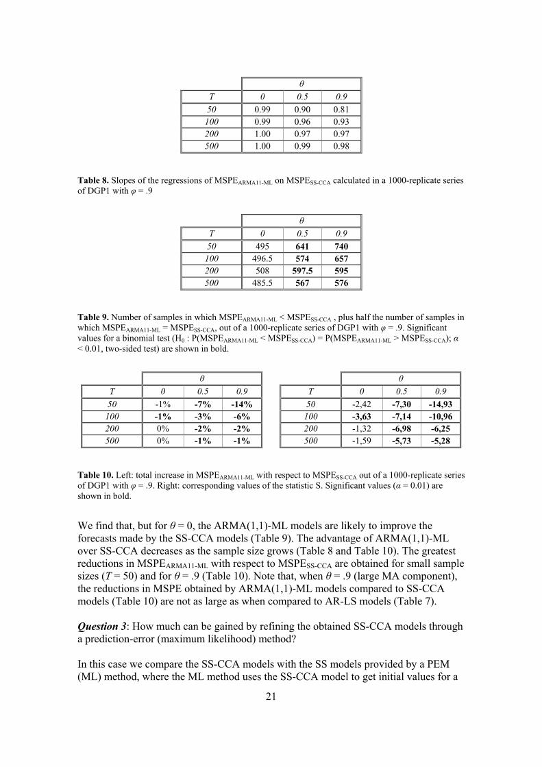
θ T 0 0.5 0.9 50 0.99 0.90 0.81 100 0.99 0.96 0.93 200 1.00 0.97 0.97 500 1.00 0.99 0.98

Table 8. Slopes of the regressions of MSPEARMA11-ML on MSPESS-CCA calculated in a 1000-replicate series of DGP1 with φ = .9

θ

T 0 0.5 0.9 50 495 641 740 100 496.5 574 657 200 508 597.5 595 500 485.5 567 576

Table 9. Number of samples in which MSPEARMA11-ML < MSPESS-CCA , plus half the number of samples in which MSPEARMA11-ML = MSPESS-CCA, out of a 1000-replicate series of DGP1 with φ = .9. Significant values for a binomial test (H0 : P(MSPEARMA11-ML < MSPESS-CCA) = P(MSPEARMA11-ML > MSPESS-CCA); α < 0.01, two-sided test) are shown in bold.

θ

T 0 0.5 0.9 50 -1% -7% -14% 100 -1% -3% -6% 200 0% -2% -2% 500 0% -1% -1%

θ T 0 0.5 0.9 50 -2,42 -7,30 -14,93 100 -3,63 -7,14 -10,96 200 -1,32 -6,98 -6,25 500 -1,59 -5,73 -5,28

Table 10. Left: total increase in MSPEARMA11-ML with respect to MSPESS-CCA out of a 1000-replicate series of DGP1 with φ = .9. Right: corresponding values of the statistic S. Significant values (α = 0.01) are shown in bold.

We find that, but for θ = 0, the ARMA(1,1)-ML models are likely to improve the forecasts made by the SS-CCA models (Table 9). The advantage of ARMA(1,1)-ML over SS-CCA decreases as the sample size grows (Table 8 and Table 10). The greatest reductions in MSPEARMA11-ML with respect to MSPESS-CCA are obtained for small sample sizes (T = 50) and for θ = .9 (Table 10). Note that, when θ = .9 (large MA component), the reductions in MSPE obtained by ARMA(1,1)-ML models compared to SS-CCA models (Table 10) are not as large as when compared to AR-LS models (Table 7). Question 3: How much can be gained by refining the obtained SS-CCA models through a prediction-error (maximum likelihood) method? In this case we compare the SS-CCA models with the SS models provided by a PEM (ML) method, where the ML method uses the SS-CCA model to get initial values for a

22

numerical search for the parameter values that minimise the sample likelihood function (Gaussian innovations).

-2 0 2 4 60

5Theta = 0

T =

50

-2 0 2 4 60

5Theta = 0.5

-2 0 2 4 60

5Theta = 0.9

-2 0 2 4 60

5

T =

100

-2 0 2 4 60

5

-2 0 2 4 60

5

-2 0 2 4 60

5

T =

200

-2 0 2 4 60

5

-2 0 2 4 60

5

-2 0 2 4 60

5

T =

500

-2 0 2 4 60

5

-2 0 2 4 60

5

Figure 9. MSPE of the forecasts of SS-ML models vs SS-CCA models in a 1000-replicate series of DGP1 with φ = .9

θ T 0 0.5 0.9 50 1.00 0.96 0.94 100 0.99 0.98 0.97 200 1.00 0.98 0.98 500 1.00 0.99 0.99

Table 11. Slopes of the regressions of MSPESS-ML on MSPESS-CCA calculated in a 1000-replicate series of DGP1 with φ = .9

MSPESS-CCA

MSP

E SS-

PEM

23

θ

T 0 0.5 0.9 50 487 557 592 100 485 550 583 200 510.5 579 576 500 479 566 563

Table 12. Number of samples in which MSPESS-ML < MSPESS-CCA , plus half the number of samples in which MSPESS-ML = MSPESS-CCA, out of a 1000-replicate series of DGP1 with φ = .9. Significant values for a binomial test (H0 : P(MSPESS-ML < MSPESS-CCA) = P(MSPESS-ML > MSPESS-CCA); α < 0.01, two-sided test) are shown in bold.

θ T 0 0.5 0.9 50 0% -3% -4% 100 -1% -2% -2% 200 0% -2% -1% 500 0% -1% -1%

θ T 0 0.5 0.9 50 -0,55 -4,64 -4,91 100 -3,14 -3,89 -3,72 200 -0,59 -4,78 -3,05 500 -1,23 -5,61 -2,96

Table 13. Left: total increase in MSPESS-ML with respect to MSPESS-CCA out of a 1000-replicate series of DGP1 with φ = .9. Right: corresponding values of the statistic S. Significant values (α = 0.01) are shown in bold.

In brief, refining the CCA estimates through a prediction-error method (which for Gaussian innovations and a quadratic loss function is equivalent to maximum likelihood) will do no harm, and when the MA component θ is not null it is likely to provide forecasts with less MSPE (Table 12). Note however that the gains in MSPE that we obtained are usually moderate (Table 13), especially for large sample sizes (T = 200, 500). The gains in MSPE obtained by ARMA(1,1)-ML models are larger than those obtained by SS-ML models, but note that in the first case we are imposing the right specification, while in the second case the SS-ML models are using the system order estimated by the CCA algorithm (Appendix II). Question 4: Are there forecasting differences between SS(1)-ML models (SS models with the right specification and PEM estimation) and ARMA(1,1)-ML models (ARMA models with the right specification and PEM estimation)?

24

-2 0 2 4 60

5Theta = 0

T =

50

-5 0 5 100

5

Theta = 0.5

-2 0 2 4 60

5Theta = 0.9

-2 0 2 4 60

5

T =

100

-2 0 2 4 60

5

-2 0 2 4 60

5

-2 0 2 4 60

5

T =

200

-2 0 2 4 60

5

-2 0 2 4 60

5

-2 0 2 4 60

5

T =

500

-2 0 2 4 60

5

-2 0 2 4 60

5

Figure 10. MSPE of the forecasts of ARMA11-ML models vs SS1-ML models in a 1000-replicate series of DGP1 with φ = .9

θ T 0 0.5 0.9 50 1.00 1.01 1.00 100 1.00 1.00 1.00 200 1.00 1.00 1.00 500 1.00 1.00 1.00

Table 14. Slopes of the regressions of MSPEARMA11-ML on MSPESS1-ML calculated in a 1000-replicate series of DGP1 with φ = .9

θ T 0 0.5 0.9 50 505 489 484.5 100 496.5 507.5 518 200 491 507 487.5 500 475.5 485.5 488

Table 15. Number of samples in which MSPEARMA11-ML < MSPESS1-ML , plus half the number of samples in which MSPEARMA11-ML = MSPESS1-ML, out of a 1000-replicate series of DGP1 with φ = .9. Significant values for a binomial test (H0 : P(MSPEARMA11-ML < MSPESS1-ML) = P(MSPEARMA11-ML > MSPESS1-ML); α < 0.01, two-sided test) are shown in bold.

MSPESS1-PEM

MSP

E AR

MA

11-P

EM

25

θ

T 0 0.5 0.9 50 0% 1% 1% 100 0% 0% 0% 200 0% 0% 0% 500 0% 0% 0%

θ T 0 0.5 0.9 50 0,40 0,97 1,37 100 1,06 -0,30 0,59 200 -0,07 -0,16 -0,95 500 0,62 0,14 -0,93

Table 16. Left: total increase in MSPEARMA11-ML with respect to MSPESS1-ML out of a 1000-replicate series of DGP1 with φ = .9. Right: corresponding values of the statistic S. Significant values (α = 0.01) are shown in bold.

The MSPE provided by SS(1)-ML and ARMA(1,1)-ML models is basically the same, as can be checked graphically on Figure 10 (note the concentration of points around the 45º line) and on the associated tables (Table 14, Table 15 and Table 16). Summary of results for DGP1 To summarize the results of our simulations with the univariate ARMA(1,1) process DGP1: - The CCA state space models provided better forecasts than the AR models when

the MA component was large (θ = .9) (see rightmost column of Table 2, Table 3 and Table 4).

- For a large MA component (θ = .9), a correct ARMA(1,1) specification would

reduce considerably and significantly the MSPE of the AR approximations (see rightmost column of Table 6 and Table 7). It would also reduce considerably and significantly the MSPE of the CCA models (Table 9 and Table 10).

- There was margin to improve the CCA models through a PEM (maximum

likelihood) method. The reductions in MSPE obtained by the refined models were in general statistically significant (Table 12 and Table 13), though moderate (less than 5 % reduction in MSPE).

- When the right specification was imposed, both the SS(1) and ARMA(1,1) models

estimated by PEM (maximum likelihood) provided basically the same predictive performance.

3.3 Data Generating Process 2 Data generating process 2 (DGP2) is a bivariate cointegrated process defined by the following equations:

(1 - L) y1,t = (1 + θ1 L) e1,t

26

y2,t = γ + β y1,t + (1 + θ2 L) e2,t where L is the lag operator and [e1,t e2,t]’ is Gaussian white noise N (0, Ω) with

⎥⎦

⎤⎢⎣

⎡=Ω

1

2

ρσρσσ

DGP2 admits the following VARMA formulation (including the constant term γ):

⎥⎦

⎤⎢⎣

⎡⎥⎦

⎤⎢⎣

⎡−

+⎥⎦

⎤⎢⎣

⎡+⎥

⎦

⎤⎢⎣

⎡=⎥

⎦

⎤⎢⎣

⎡⎥⎦

⎤⎢⎣

⎡−⎥

⎦

⎤⎢⎣

⎡

−

−

−

−

1,2

1,1

221

1

,2

,1

1,2

1,1

,2

,1

)(00

001

t

t

t

t

t

t

t

t

uu

uu

yy

yy

θθθβθ

γβ

where ⎥⎦

⎤⎢⎣

⎡⎥⎦

⎤⎢⎣

⎡=⎥

⎦

⎤⎢⎣

⎡

t

t

t

t

ee

uu

,2

,1

,2

,1

101

β

Searching for a variety of statistical properties in the generated processes we selected the parameter space θ1 = .5, .9 ; θ2 = .5, .9 ; β = 1 ; ρ = 0, .8 ; σ = 1, 2; γ = 50. For different sample sizes T = 100, 200, 400, 800 and for every combination of the values (T, θ1, θ2, β, φ, σ), we generate 1000 samples from which we obtain (1000 pairs of) results for the one-step-ahead quality of prediction indicators (MSPEVAR, MSPECCA), measured for 10 new observations of every sample and recalculating the models as the new observations are included. Note that for DGP2 the cointegrating relation is

y2,t - β y1,t = γ + (1 + θ2 L) e2,t so there is a constant term (γ) in the cointegrating relation. The VAR or vector error-correction (VEC) models are calculated by Johansen’s procedure adapted for the case of constant terms in the cointegrating relations and no deterministic trends, as described in Appendix I. The correct number of stochastic common trends (i.e. one) has been imposed for Johansen’s models. For the subspace models, we start by eliminating the effect of the constant term γ, centring the data (subtracting the average values); thus, the following relation is obtained:

(y2,t - Ty ,2 ) - β (y1,t - Ty ,1 ) = e2,t + θ2 e2,t-1 – ( Te ,2 + θ2 1,2 −Te ) where Tx stands for the sample average of variable x up to time T. Representative results of our simulations are shown in Figure 11, Table 17and Table 18. The relative advantage of one method over the other depends on the values of the parameters of the DGP and on the particular series (y1,t or y2,t). In the case of y1,t

27

significant advantages of the CCA models over the VEC models are obtained for sample sizes greater than 100 and for θ1 = .9. In the case of y2,t, significant advantages of the CCA models over the VEC models are obtained for sample sizes greater than 100 and for (θ2 = .9, σ = 1 ) or (θ1 = .9, σ = 2). On the other hand, significant advantages of the VEC models over the CCA models are usually obtained when forecasting with sample size 100 or 200 and using the small values of θj.

0 2 40

2

4

T = 100

Thet

a1 =

0.5

Thet

a2 =

0.5

0 2 40

2

4

Thet

a1 =

0.5

Thet

a2 =

0.9

0 2 40

2

4

Thet

a1 =

0.9

Thet

a2 =

0.5

0 2 40

2

4

Thet

a1 =

0.9

Thet

a2 =

0.9

0 1 2 30

1

2

3

T = 200

0 1 2 30

1

2

3

0 2 40

2

4

0 1 2 30

1

2

3

0 1 2 30

1

2

3

T = 400

0 2 40

2

4

0 2 40

2

4

0 1 2 30

1

2

3

0 1 2 30

1

2

3T = 800

0 1 2 30

1

2

3

0 1 2 30

1

2

3

0 1 2 30

1

2

3

Figure 11. MSPECCA and MSPEVEC for y1,t in a 1000-replicate series of DGP2 with σ = 1 and ρ = .8.

y1 y2

θ1 θ2 T=100 200 400 800 T=100 200 400 800 0.5 0.5 359 441 454 482 345 434 458 468

0.9 436 452 498 511.5 548 519.5 571 565 0.9 0.5 549 578 618 591 441 524 551 572

0.9 539.5 605 607 598 539 625 607 609

Table 17. Number of samples in which MSPECCA < MSPEVEC , plus half the number of samples in which MSPECCA = MSPEVEC, out of a 1000-replicate series of DGP2 with β = 1, σ = 1 and ρ = .8. Significant values for a binomial test (H0 : P(MSPECCA < MSPEVEC) = P(MSPECCA > MSPEVEC); α = 0.01, two-sided test) are shown in bold.

MSPEVEC

MSP

E CC

A

28

y1 y2 θ1 θ2 T=100 200 400 800 T=100 200 400 800 0.5 0.5 10% 4% 2% 1% 11% 4% 2% 1%

0.9 6% 3% 0% 0% -1% -1% -2% -1% 0.9 0.5 -3% -4% -5% -3% 3% 0% -2% -2%

0.9 -2% -5% -4% -3% -2% -5% -4% -3%

y1 y2 θ1 θ2 T=100 200 400 800 T=100 200 400 800 0.5 0.5 12,18 6,54 4,33 2,30 12,98 7,21 4,59 2,29

0.9 7,08 4,25 0,80 0,44 -1,02 -2,44 -5,50 -4,48 0.9 0.5 -3,42 -5,67 -9,67 -7,61 3,60 -0,42 -4,91 -4,49

0.9 -2,40 -7,50 -7,32 -7,24 -1,90 -8,57 -7,98 -7,58

Table 18. Top table: total increase in MSPECCA with respect to MSPEVEC out of a 1000-replicate series of DGP2 with β = 1, σ = 1 and ρ = .8. Bottom table: corresponding values of the statistic S. Significant values (α = 0.01) are shown in bold.

Table 19 shows some results corresponding to the Adapted Canonical Correlation Analysis (ACCA) models of Bauer and Wagner (2002). Although, within the considered algorithms, consistent estimation of all system parameters of VARMA cointegrated systems has only been proven for the ACCA algorithm, in our simulations, the ACCA models did not show predictive advantages over the CCA models (the ACCA models showed similar performance to the CCA models; they were better in some occasions but worse in some others). Augmenting the prediction horizon usually involves gradual little changes in the tournament results. In general, as in Bauer and Wagner (2003), we found a relative improvement in the performance of Johansen’s model as the prediction horizon grows, probably because this model imposes a value of exactly 1 for the non stationary roots (which is the right value for our simulated processes). However, the unit root restrictions can also be considered in the subspace model through a reduced-rank regression in the estimation of the state transition matrix (Reinsel and Velu 1998; Bauer and Wagner 2002), imposing that the rank of (A - In ) must be (n - c), where n is the order of the model and c is the number of common trends. The results of Bauer and Wagner (2003) also raise concerns about the performance of subspace algorithms compared to Johansen’s method when the number of series in yt gets large.

29

y1 y2 θ1 θ2 T=100 200 400 800 T=100 200 400 800 0.5 0.5 16% 7% 3% 1% 5% 3% 2% 1%

0.9 27% 18% 12% 7% 4% 2% 1% 0% 0.9 0.5 26% 16% 8% 5% 7% 4% 1% 1%

0.9 24% 15% 10% 7% 3% 0% 0% 0%

y1 y2 θ1 θ2 T=100 200 400 800 T=100 200 400 800 0.5 0.5 15,45 11,30 7,84 5,25 8,30 7,53 5,64 3,16

0.9 20,26 19,39 17,49 13,00 5,12 4,13 2,51 0,79 0.9 0.5 18,48 16,10 11,77 9,33 9,60 6,81 3,34 1,87

0.9 16,48 14,84 13,32 11,73 3,61 -0,43 -0,20 -0,68

Table 19. Top table: total increase in MSPEACCA with respect to MSPEVEC out of a 1000-replicate series of DGP2 with β = 1, σ = 1 and ρ = .8. Bottom table: corresponding values of the statistic S. Significant values (α = 0.01) are shown in bold.

Summary of results for DGP2 DGP2 is a VARMA bivariate cointegrated process used to compare the forecasting accuracy of Johansen’s VEC models with that of SS CCA models. Our results show that the MA components have a large influence on the relative finite-sample performance of both methods. In our experiments, large values (close to 1) of the MA components usually led to relative advantages for the SS CCA models. 4. A practical case In this section we compare, for two cointegrated series of real data, the point and density forecasts made by CCA models with those made by Johansen’s VAR models. We take a series of 4,805 crude oil daily prices between January 1986 and March 2005, as well as the corresponding “oil future contract” prices. The data is freely provided by the U.S. Energy Information Administration in their web page. The spot prices correspond to “Cushing, OK WTI Spot Price FOB ($/bbl)” and the future prices to “Cushing, Ok Crude Oil Future Contract 4 ($/bbl)”. Instead of working directly with prices, whose variations have a lower bound and are expected to be proportional to the price level, we take the logarithms of the original data: y1 = log(spot), y2 = log(future). The sample is shown in Figure 12.

30

Jan 1986 March 20052.2

2.4

2.6

2.8

3

3.2

3.4

3.6

3.8

4

4.2

Figure 12. The studied sample: log(spot) and log(future).

The autocorrelogram and partial autocorrelogram for the series log(spot) and log(future) are shown in Figure 13.

0 10 20 30-0.5

0

0.5

1

Aut

ocor

rela

tion

log(spot)

0 10 20 30-0.5

0

0.5

1log(future)

0 10 20 30-0.5

0

0.5

1

Lag

Par

tial A

utoc

orre

latio

ns log(spot)

0 10 20 30-0.5

0

0.5

1

Lag

log(future)

Figure 13. Autocorrelogram and partial autocorrelogram for the series log(spot)-left- and log(future)-right-.

For both series, if we assume no deterministic trend, the augmented Dickey-Fuller test with 1 lag (this number of lags was selected to eliminate correlation in the residuals), as well as the Philips-Perron test, do not reject the null of a unit root at the 5% level (Table

31

20). However, there seemed to be conditional heterocedasticity in the residuals of the regressions made by both tests. ADF Test Statistics 1% Critical Value* -3.4349 Log(future) -1.891829 5% Critical Value -2.8627 Log(spot) -2.698352 10% Critical Value -2.5674

PP Test Statistic 1% Critical Value* -3.4349 Log(future) -2.058627 5% Critical Value -2.8627 Log(spot) -2.418566 10% Critical Value -2.5674

*MacKinnon critical values for rejection of hypothesis of a unit root. Lag truncation for Bartlett kernel: 9 ( Newey-West suggests: 9 )

Table 20. ADF and PP tests for log(future) and for log(spot). ADF test made with one lag plus constant.

A Johansen cointegration test (Table 21) with a VAR(1) specification indicates one cointegrating equation. Test assumption: No deterministic trend in the data Lags interval: 1 to 1

Likelihood 5 Percent 1 Percent Hypothesized Eigenvalue Ratio Critical Value Critical Value No. of CE(s) 0.018872 89.29129 19.96 24.60 None ** 0.000817 3.671838 9.24 12.97 At most 1

*(**) denotes rejection of the hypothesis at 5%(1%) significance level L.R. test indicates 1 cointegrating equation(s) at 5% significance level

Normalized Cointegrating Coefficients: 1 Cointegrating Equation(s) LOGSPOT LOGFUTURE C 1.000000 -1.065687 0.178895

(0.02091) (0.06332) Table 21. Results of the Johansen cointegration test. The numbers in parentheses under the estimated coefficients are the asymptotic standard errors.

If, alternatively, we expected the cointegrating relation to be log(spot) = log(future) + st, with st being stationary, we can test whether the log(spot) - log(future) differences are stationary. Both the Dickey-Fuller test (Statistic = -6.286, 1% Critical Value = -3.435) and the Philips-Perron test (Statistic = -7.923, 1% Critical Value = -3.435) reject the null hypothesis of a unit root on the difference series st, at the 1 % level (but again there seems to exist conditional heterocedasticity in the residuals of the regressions used by these tests). We now compare the forecasts made by the CCA models and by Johansen’s models. We start the system-identification process using the first 1,000 observations. As the time index advances, both models are re-calculated (i.e. specified and estimated) with all the past data, and the one-step-ahead density forecasts are computed according to the updated models. For almost every t the selected VAR (AIC criterion) resulted of order 1

32

and the selected CCA model resulted of order 2. It can be seen in Table 22 that the MSE and MAE of the one-step-ahead predictions is almost the same for both models, but it is also almost the same (even less) for the random walk model ŷt|t-1 = yt-1.

MSPE (1.0 e-7 *) MAPE(1.0 e-4 *) y1 y2 y1 y2 CCA 6589 3361 177 129 VAR 6565 3360 176 128 Random Walk 6591 3355 176 128

Table 22. Mean Square Prediction Error and Mean Absolute Prediction Error for the different models and series.

The null hypothesis of “equal forecast accuracy” E (MSPECCA) = E (MSPEVAR) was tested using the Diebold-Mariano and the Morgan-Granger-Newbold tests. Note that these tests are not the same as those used in the simulation study, because when simulating we can obtain as many time series as desired from the same DGP, but now we only have one single (bivariate) time series. The results can be seen in Table 23: the data strongly supports the “equal forecast accuracy” hypothesis.

Diebold-Mariano Morgan-Granger-Newbold y1 y2 y1 y2 Statistic 222 e-4 795 e-6 180 e-3 620 e-5 p-value 0.982 0.999 0.857 0.995

Table 23. Results of the Diebold-Mariano and Morgan-Granger-Newbold tests for “equal forecast accuracy”.

The series of one-step-ahead prediction errors (see Figure 14 for some of these series) do not show autocorrelation, but conditional heterocedasticity seems to be visible in the graphs, as well as in the autocorrelation of the squared centred residuals. A CUSUM test (Brown, Durbin and Evans 1975) for the VAR prediction errors for each series (see Figure 15) would not reject the hypothesis of structural stability (significance level 0.05). However, neither the VAR nor the CCA models allow for conditional heterocedasticity, so we may expect “bad” density forecasts in both cases.

33

500 1000 1500 2000 2500 3000 3500 4000-0.4

-0.2

0

0.2

one-step-ahead prediction error for log(spot), VAR models

0 500 1000 1500 2000 2500 3000 3500 4000-0.4

-0.2

0

0.2

one-step-ahead prediction error for log(spot),CCA models

0 2 4 6 8 10 12 14 16 18 20-0.5

0

0.5

1

Sam

ple

Aut

ocor

rela

tion

Autocorrelations of one-step-ahead prediction errors for log(spot), CCA models

0 2 4 6 8 10 12 14 16 18 20-0.5

0

0.5

1

Lag

Autocorrelations of squared one-step-ahead prediction error for log(spot), CCA models

Figure 14. One-step-ahead prediction errors for the log(spot) series using the VAR and CCA models. The middle graph shows the sample autocorrelations of the CCA errors (similar graphs for the VAR errors) and the bottom graph shows the sample autocorrelations of the squared centred errors.

0 500 1000 1500 2000 2500 3000 3500 4000-300

-200

-100

0

100

200

300

Figure 15. Cumulative sum of standardised VAR prediction errors for log(spot) and log(future), together with the 95 % and 99 % confidence bands for a CUSUM test for the individual series.

Observation number

Cum

ulat

ive

stan

dard

ised

err

or

34

Density forecasting We may be interested not only in point estimates of future values, (e.g. forecasts of yt|t-

1), but also in estimates of the probability distribution of those future values (e.g. density forecasts of yt|t-1). There is a growing literature on density forecasting (Tay and Wallis 2000). Statistical evaluation of density forecasts is usually based on the probability integral transform: Let ft-1(y) be the probability density function of yt conditional on past information up to time t-1. Then, the probability integral transforms of yt with respect to ft-1(y), defined by

zt = ∫ ∞− −ty

t dxxf )(1 ,

are independent uniform U[0,1] variates (Diebold, Gunther and Tay 1998). So, given the sample (y1, …, yT) and the one-step-ahead density forecasts )(ˆ

1 xft− , the

idea in order to asses the quality of the density forecasts is to calculate zt = ∫ ∞− −ty

t dxxf )(ˆ1

(t = 1, …, T) and check whether the zt are independent U[0,1]. The independence of zt can be checked through the autocorrelograms of the centred moments. Uniformity is usually checked using graphs and analytical tests: plotting the cumulative distribution function and (assuming independence) using a test such as Kolmogorov-Smirnov’s (Clements and Smith 2000), or plotting a histogram and using a binomial test for the number of data in a bin (Diebold, Gunther and Tay 1998). The latter authors discuss extensions to multivariate forecasts (see also Diebold, Hahn and Tay 1999) and to multi-step-ahead forecasts, as well as causes of departure from i.i.d. U[0,1]. The approach in the multivariate case consists in decomposing the multivariate density into the product of marginal and conditional univariate densities, based on the relation

ft-1(y1t, y2t, …, yNt) = ft-1(yNt| y1t, y2t, …, yN-1,t) ··· ft-1(y2t| y1t) ft-1(y1t). We now try to assess the quality of the one-step-ahead density forecasts made by the different estimated models in our bivariate case. We follow mainly Clements and Smith (2000), who provide a multivariable and multi-step-ahead study in which density forecasts are used to discriminate between competing models. For model m (m = CCA, Johansen) we consider the density forecasts yt|t-1 ~ fm

t-1(y1t, y2t) ≡ N(ŷmt|t-1, Σm), where

⎥⎦

⎤⎢⎣

⎡∑∑∑∑

=∑2221

1211m

is the covariance matrix of the innovations (yt - ŷm

t|t-1) according to model m. We factor the joint density into the product of the conditional and marginal:

35

f(y1t, y2t) = f(y1t| y2t) f(y2t) = f(y2t| y1t) f(y1t). To make notation simpler, let (ŷm

1, ŷm2) be the components of ŷm

t|t-1. The conditional fmt-

1(y1t| y2t) is

N ﴾ ŷm1 +

22

21

ΣΣ (y2t - ŷm

2) , Σ11 (1 – ρ2) ﴿, where ρ = ( ) 2/1

2211

21

ΣΣΣ

and the marginal fm

t-1(y2t) is N (ŷm2, Σ22).

Now, with the actual data yt we obtain, for every model, the probability integral transforms z1|2 from the conditionals fm

t-1(y1t| y2t), and z2 from the marginals fmt-1(y2t). If

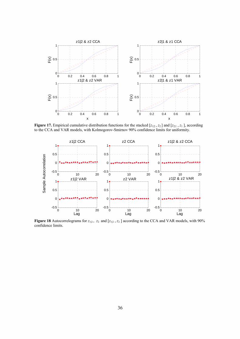
the multivariate density forecasts are correct, both series should be iid U[0,1], individually and also when taken as a whole (Diebold, Hahn and Tay 1999). Similarly, we can obtain z2|1 and z1, as well as the stacked [z2|1 , z1], and check whether they are iid U[0,1]. Using our series of oil prices, the probability integral transforms provide, for the CCA and Johansen’s models, the series z1|2, z2, z2|1 and z1, whose independence and uniformity (as well as that of the stacked pairs z1|2 U z2 and z2|1 U z1) can be assessed through graphs and tests. Figure 16 shows histograms for the marginals, with 90% confidence limits for the number of observations in a bin. Figure 17 shows the cumulative distribution functions for the stacked pairs, with Kolmogorov-Smirnov 90% confidence limits for the U[0,1] hypothesis (assuming independence). Figure 18 and Figure 19 show autocorrelation plots for the two first centred moments of some of the variables. According to the obtained results, independence and uniformity of the z transforms would be rejected for both the CCA and VAR models but, again, their density forecasting performance seems to be very similar.

0 0.2 0.4 0.6 0.8 10

200

400z1 CCA

0 0.2 0.4 0.6 0.8 10

200

400z2 CCA

0 0.2 0.4 0.6 0.8 10

200

400z1 VAR

0 0.2 0.4 0.6 0.8 10

200

400z2 VAR

Figure 16. Histograms for z1 and z2, according to the CCA and VAR models, with 90% confidence limits for a binomial test on the number of observations in a bin.

36

0 0.2 0.4 0.6 0.8 10

0.5

1F(

x)

z1|2 & z2 CCA

0 0.2 0.4 0.6 0.8 10

0.5

1

F(x)

z2|1 & z1 CCA

0 0.2 0.4 0.6 0.8 10

0.5

1

x

F(x)

z1|2 & z2 VAR

0 0.2 0.4 0.6 0.8 10

0.5

1

x

F(x)

z2|1 & z1 VAR

Figure 17. Empirical cumulative distribution functions for the stacked [z1|2 , z2 ] and [z2|1 , z1 ], according to the CCA and VAR models, with Kolmogorov-Smirnov 90% confidence limits for uniformity.

0 10 20-0.5

0

0.5

1z1|2 CCA

0 10 20-0.5

0

0.5

1z2 CCA

0 10 20-0.5

0

0.5

1z1|2 & z2 CCA

0 10 20-0.5

0

0.5

1

Lag

Sam

ple

Aut

ocor

rela

tion

z1|2 VAR

0 10 20-0.5

0

0.5

1

Lag

z2 VAR

0 10 20-0.5

0

0.5

1

Lag

z1|2 & z2 VAR

Figure 18 Autocorrelograms for z1|2 , z2 and [z1|2 , z2 ] according to the CCA and VAR models, with 90% confidence limits.

37

0 10 20-0.5

0

0.5

1square z1|2 CCA

0 10 20-0.5

0

0.5

1square z2 CCA

0 10 20-0.5

0

0.5

1 square z1|2 & z2 CCA

0 10 20-0.5

0

0.5

1

Lag

Sam

ple

Aut

ocor

rela

tion

square z1|2 VAR

0 10 20-0.5

0

0.5

1

Lag

square z2 VAR

0 10 20-0.5

0

0.5

1

Lag

square z1|2 & z2 VAR

Figure 19 Autocorrelograms for the square values of z1|2 , z2 and [z1|2 , z2 ] according to the CCA and VAR models, with 90% confidence limits.

We should turn to other models (e.g. GARCH) that allow for conditional heterocedasticity. However, if we just modify our estimate of the error covariance matrix at time t by taking the sample error covariance of the last two weeks (other window sizes were tested, with this one giving good results), then the density forecasts of the CCA and Johansen’s models improve considerably, as seen in Figure 20 to Figure 23 (though the models would not be using the variance information for efficient parameter estimation).

0 0.2 0.4 0.6 0.8 10

100

200

300z1 CCA

0 0.2 0.4 0.6 0.8 10

100

200

300z2 CCA

0 0.2 0.4 0.6 0.8 10

100

200

300z1 VAR

0 0.2 0.4 0.6 0.8 10

100

200

300z2 VAR

Figure 20. Histograms for z1 and z2, according to the CCA and VAR models with dynamic error variance, with 90% confidence limits for a binomial test on the number of observations in a bin.

38

0 0.2 0.4 0.6 0.8 10

0.5

1

F(x)

z1|2 & z2 CCA

0 0.2 0.4 0.6 0.8 10

0.5

1

F(x)

z2|1 & z1 CCA

0 0.2 0.4 0.6 0.8 10

0.5

1

x

F(x)

z1|2 & z2 VAR

0 0.2 0.4 0.6 0.8 10

0.5

1

xF(

x)

z2|1 & z1 VAR

Figure 21. Empirical cumulative distribution functions for the the stacked [z1|2 , z2 ] and [z2|1 , z1 ], according to the CCA and VAR models with dynamic error variance, with Kolmogorov-Smirnov 90% confidence limits for uniformity.

0 10 20-0.5

0

0.5

1z1|2 CCA

0 10 20-0.5

0

0.5

1z2 CCA

0 10 20-0.5

0

0.5

1z1|2 & z2 CCA

0 10 20-0.5

0

0.5

1

Lag

Sam

ple

Aut

ocor

rela

tion

z1|2 VAR

0 10 20-0.5

0

0.5

1

Lag

z2 VAR

0 10 20-0.5

0

0.5

1

Lag

z1|2 & z2 VAR

Figure 22. Autocorrelograms for z1|2 , z2 and [z1|2 , z2 ] according to the CCA and VAR models with dynamic error variance, with 90% confidence limits.

39

0 10 20-0.5

0

0.5

1square z1|2 CCA

0 10 20-0.5

0

0.5

1square z2 CCA

0 10 20-0.5

0

0.5

1square z1|2 & z2 CCA

0 10 20-0.5

0

0.5

1

Lag

Sam

ple

Aut

ocor

rela

tion

square z1|2 VAR

0 10 20-0.5

0

0.5

1

Lag

square z2 VAR

0 10 20-0.5

0

0.5

1

Lag

square z1|2 & z2 VAR

Figure 23. Autocorrelograms for the square values of z1|2 , z2 and [z1|2 , z2 ] according to the CCA and VAR models with dynamic error variance, with 90% confidence limits.

Summary of results for the practical case In short, the CCA models and Johansen’s VAR (VEC) models provide basically the same forecasting performance in our real case. As we showed in section 3, experiments with known VARMA DGPs can detect significant differences in forecasting performance under certain conditions (system parameters, sample sizes) that are associated to the MA components of the model, and it is possible to check for those conditions in real systems. However, it may also be difficult to find real series whose behaviour is in accordance with our desired laboratory conditions, specially when, as it happens in our practical case, even linear models with (conditional) constant parameters may only be able to provide “reasonable” approximations to the real process. Anyway, there is also no a priori reason why in a real case the VARMA representation of (or approximation to) the true generating process should not have large MA components. 5. Conclusions VAR models present some advantages over VARMA modelling that make them an attractive option: the system specification is easier to conduct (fewer hyperparameters to estimate) and the maximum likelihood parameter estimates can be obtained by least squares (LS) quickly in a single step (non-iterative estimation, no need for a numerical optimization). For state space (SS) modelling, subspace algorithms also provide quick and non-iterative estimates, and an even simpler specification procedure. Finite VAR models can only approximate VARMA processes (with MA components), whereas finite state space models can provide exact representations. Based on this feature, we expected that subspace-based SS models of VARMA processes could provide better forecasts than VAR models of the same processes. Our simulation results suggest that, for univariate ARMA(1,1) processes with a considerable weight of the MA component (a value close to 1), state space CCA models are indeed likely to provide forecasts with less Mean Squared Prediction Error (MSPE) than AR-LS models. In our univariate cases this comparatively better performance of

40

CCA models was only achieved for sample sizes not too small (from 100 observations). It is frequently remarked that subspace estimates can or should be refined through a prediction-error method PEM (if speed is not a critical factor), and we provide some examples of the gains in forecasting performance obtained in this way. Note that by selecting an iterative PEM, part of the speed advantages of subspace methods would be lost, but they would still provide a quick specification for a state space model, as well as good initial estimates for the iterative PEM search. For several simulated ARMA processes we have quantified the forecasting accuracy of ARMA_ML, VAR_LS, SS_CCA and SS_ML estimated models, providing some references on the magnitude of the possible gains/losses in predictive power among these methods. Quantified comparisons are often difficult to find in the literature and can provide a guidance as to the convenience (cost/ possible benefit) of obtaining different models for a given time series. In our simulations, ARMA_ML and SS_ML provided the best (and basically the same) forecasting performance but, computationally, these are the most involved methods, and they require numerical iterative techniques. For multivariate time series, state-space-based system-identification methods present some additional advantages over VARMA modelling, especially for the specification step: there is only one hyperparameter to estimate, namely the order n of the state-space model. In our comparison between SS and VAR models we focused in cointegrated systems because these processes are usually analysed using VAR models. For VARMA cointegrated processes we presented some simulation results comparing the predictive performance of Johansen’s VAR models with the predictive performance of subspace-based state space models. Our results for some simple bivariate cases indicate small predictive differences, but in several cases subspace models showed significant advantages over VAR models when the VARMA processes were simulated using high (close to 1) values for the MA components. In brief, our results supported our initial hypothesis about SS-CCA models providing better forecasts than VAR-LS models for VARMA processes with “large” MA components. After having detected these forecasting differences between SS and VAR models, an interesting question for future research is what data features (statistics) can a priori indicate which modelling method is more appropriate for a given series of data. Meanwhile, when dealing with a particular problem, it is advisable to try different modelling approaches, and subspace methods, as well as VAR_LS, provide “cheap” alternatives. In our practical case both the subspace models and Johansen’s VAR (VEC) models provided basically the same (density) forecasting performance, but since subspace models can be obtained quickly and easily, and given that, as we show in this paper, there can be statistically significant differences in their forecasting performance with the alternative VAR models, we consider that it can be good practice to complement VAR models with subspace-based state space models when forecasting real processes. Besides, from a structural point of view, state space models could be open to economic analysis and interpretations of the system dynamics through suitable rotations of the

41

state vector (thus exposing and composing/decomposing the dynamic components in convenient ways). Acknowledgements The authors would like to thank Dr. Dietmar Bauer for kindly providing some preliminary MATLAB® code for the subspace CCA and ACCA algorithms. We would also like to thank comments from two anonymous referees to a reduced version of this paper.

42

Appendix I Johansen’s method Let yt be a cointegrated vector made up by m individually I(1) series which follows a VAR of order p:

yt = α + Ф1 yt-1 + Ф2 yt-2 + ... + Фp yt-p + et where et is a (m × 1) white noise vector N(0, Ω). Then yt can equivalently be written in vector error correction (VEC) form as

Δyt = ζ1 Δyt-1 + ζ2 Δyt-2 + ... + ζp-1 Δyt-p+1 + α + ζo yt-1 + et

and the cointegrating relations can be obtained from ζo, whose rank is the number of cointegrating relations. Johansen (1988) derived the maximum likelihood (assuming Gaussian innovations) estimates of the system parameters (Ω, ζ1, ζ2,..., ζp-1, α, ζo ) subject to different rank restrictions for ζo, which allows for likelihood ratio tests on the number of cointegrating relations. The method proceeds in three stages: calculate auxiliary regressions, calculate canonical correlations of the residuals of the auxiliary regressions and calculate maximum likelihood estimates of parameters. The algorithm we implemented for Johansen’s method, for a system with constant terms in the cointegrating relations and without deterministic terms, follows Hamilton (1994, p. 643):

Step 1: Calculate Auxiliary Regressions:

1) A regression of Δyt on (Δyt-1, Δyt-2,..., Δyt-p+1) with no constant term,

Δyt = Π1 Δyt-1+ Π2 Δyt-2 + ... + Πp-1 Δyt-p+1 + ut

2) A regression of a constant term on (Δyt-1, Δyt-2,..., Δyt-p+1),

1 = ω’1 Δyt-1+ ω’2 Δyt-2 + ... + ω’p-1 Δyt-p+1 + wt

3) A regression of yt-1 on (Δyt-1, Δyt-2,..., Δyt-p+1) with no constant term,

yt-1 = ℵ1 Δyt-1+ ℵ2 Δyt-2 + ... + ℵp-1 Δyt-p+1 + vt

Step 2: Calculate Canonical Correlations With the residuals ut, wt and vt from the previous step build the vector wt = [wt, v’t]’ and calculate the sample covariance matrices

Σww = (1/T)∑=

T

t 1 wt w’t

43

Σuu = (1/T)∑=

T

t 1 ut u’t

Σuw = (1/T)∑=

T

t 1 ut w’t

Calculate the (n+1) × (n+1) matrix Σww

-1 Σwu Σuu-1 Σuw and its eigenvalues: λ1 > λ2 > ...

> λn+1. The maximum value achieved for the log likelihood function subject to the constraint that there are h cointegrating relations (rank(ζo) = h) and no deterministic time trends is

Lh = – (Tn/2) log(2π) – (Tn/2) – (T/2) log|Σuu| – (T/2) ∑=

h

i 1

log (1- λi )

Step 3. Calculate Maximum Likelihood Estimates of Parameters

Let a1, a2,..., an+1 denote the eigenvectors of Σww

-1 Σwu Σuu-1 Σuw corresponding to the

eigenvalues λ1 > λ2 > ... > λn+1 , normalized by the condition a’i Σww ai = 1. Let à be the matrix [a1, a2,..., ah]. Then, the maximum likelihood estimates of α and ζo are

[ 0ˆˆ ζα ] = Σuw à Ò

The maximum likelihood estimate of each ζi is

iζ = Πi - α ω’i - 0ζ ℵi for i = 1, 2, …, p-1, and the maximum likelihood estimate of Ω is

Ω = (1/T) ∑=

T

t 1[(ut - α wt - 0ζ vt) (ut - α wt - 0ζ vt)’]

Appendix II Implementation of the CCA algorithm The original data is a (m × 1) vector time series yt, with t = 1, 2, …, T. The objective is to obtain estimates of the state space system matrices A, C and K, and the covariance matrix R. CCA is based on a Canonical Correlation Analysis (Takane, Yanai and Hwang 2006) between Yf and Yp (see section 2). Parameters p and f of the orthogonal projection yt

f / yt-1p were selected as p = f = 2 × ρ,

where ρ is the order selected for a VAR representation of the data according to the Akaike information criterion (see Bauer and Wagner 2002 for a justification of these values). Both p and f were not allowed to be greater than T/3 in the univariate cases or greater than T/5 in the bivariate cases, where T is the total number of observations (this is in order to prevent possible invertibility problems in some of the matrices).

44

For t = 1, 2, …, T-p-f+1, the (m·f × T-p-f+1) matrix Yf was created from yt, so that the tth column of Yf is yp+t

f ≡ [yp+t’, yp+t+1’, ..., yp+t+f-1’]’,. For t = 1, 2, …, T-p+1, the (m·p × T-p+1) matrix Yp was created from yt, so that the tth column of Yp is yt+p-1

p ≡ [yt+p-1’, yt+p-2’, ..., yt’]’. The (m·p × T-p-f+1) matrix Ypp was created by taking the first T-p-f+1 columns of Yp. Following the estimation approach of Bauer and Wagner (2002), the conditioned (weighted) matrix W corresponding to the CCA algorithm was calculated as

W = (Yf Y’f)–1/2 (Yf Y’pp) (Ypp Y’pp) –1 (Ypp Y’pp) 1/2 where X1/2 denotes the Cholesky factor of the positive definite matrix X such that X1/2 (X1/2)’ = X. A singular value decomposition of W was performed: W = U S V, where S is a diagonal matrix which contains the singular values of W in its diagonal in decreasing order. The order of the state space model was estimated by the BA(n) criterion of Bauer and Wagner (2003)4: we choose the order n that minimises

BA(n) = - log ( 1- 21ˆ +nσ ) + 2nm log(T) / T

where m is the number of time series (row dimension of yt), T is the sample size and 2ˆ iσ is the ith largest singular value of the conditioned matrix of the CCA algorithm. A matrix of estimated estates Z = [zp+1|p, zp+2|p+1... zT+1|T] was calculated as Z = Sn

1/2 Vn (Ypp Y’pp) -1/2 Yp , where Sn is a (n × n) diagonal matrix which contains the first (highest) n singular values of W, (i.e., Sn contains the first n columns and rows of S) and Vn is a (n × m·p) matrix which contains the first n columns of V. Based on the relation yt = C zt + et , the matrix C and the residuals [ep+1, ep+2, ..., eT] were estimated by regressing [yp+1, yp+2, ..., yT] on [zp+1|p, zp+2|p+1... zT|T-1]. The covariance matrix R was estimated by the covariance matrix of the estimated residuals. Based on the relation zt+1 = A zt + K et , the matrices A and K were estimated by regressing [zp+2|p+1, zp+3|p+2, ..., zT+1|T] on [zp+1|p, zp+2|p+1, ..., zT|T-1] and on the estimated [ep+1, ep+2, ..., eT].

4 Another interesting option to select the order would be the corrected variant of AIC proposed by Bengtsson and Cavanaugh (2006) for state space models.

45

References Aoki, M., 1990. State Space Modeling of Time Series. Second, Revised and Enlarged Edition. Springer-Verlag.

Aoki, M. and Havenner, A., 1991. State Space Modeling of Multiple Time Series. Economet. Rev. 10 (1), 1-59.

Bauer, D., 2005a. Asymptotic Properties of Subspace Estimators. Automatica 41 (3), 359-376.

Bauer, D., 2005b. Comparing the CCA Subspace Method to Pseudo Maximum Likelihood Methods in the case of No Exogenous Inputs. J. Time Series Analysis 26 (5), 631-668.

Bauer, D. and Ljung, L., 2002. Some Facts about the Choice of the Weighting Matrices in Larimore Type of Subspace Algorithms. Automatica 38 (5), 763-773. Bauer, D. and Wagner, M., 2002. Estimating Cointegrated Systems using Subspace Algorithms. J. Econometrics 111, 47-84. Bauer, D. and Wagner, M., 2003. The Performance of Subspace Algorithm Cointegration Analysis: A Simulation Study. Working paper, University of Bern. Bengtsson, T. and Cavanaugh, J.E., 2006. An improved Akaike Information Criterion for State-space Model Selection. Comput. Stat. Data An. 50 (10), 2635-2654. Brown, R. Durbin, J. and Evans, J., 1975. Techniques for Testing the Constancy of Regression Relationships over Time. J. Roy. Stat. Soc. B 37, 149-172. Clements, M.P. and Smith, J., 2000. Evaluating the Forecast Densities of Linear and Non-linear Models: Applications to Output Growth and Unemployment. J. Forecasting 19, 255-276. De Cock, K. and De Moor, B., 2003. Subspace Identification Methods, in Contribution to section 5.5, “Control systems robotics and automation” of EOLSS, UNESCO Encyclopedia of Life Support Systems, (Unbehauen H.D.), vol. 1 of 3, Eolss Publishers Co., Ltd. (Oxford, UK), 933-979. Diebold, F.X., Günther T.A. and Tay, A.S., 1998. Evaluating Density Forecasts with Applications to Financial Risk Management. Int. Econ. Rev. 39 (4), 863-883. Diebold, F.X., Hahn, J. and Tay, A.S., 1999. Multivariate Density Forecast Evaluation and Calibration in Financial Risk Management: High Frecuency Returns on Foreign Exchange. Rev. Econ. Stat. 81, 661-673. Diebold, F.X. and Mariano, R.S., 2002. Comparing Predictive Accuracy. J. Bus. Econ. Stat. 20 (1), 134-44.

46

Godolphin, E.J. and Triantafyllopoulos, K., 2006. Decomposition of Time Teries Models in State-space Form. Comput. Stat. Data An. 50 (9), 2232-2246. Hamilton, J.D., 1994. Time Series Analysis. Princeton University Press. Hannan, E. and Deistler, M., 1988. The Statistical Theory of Linear Systems. Wiley, New York. Harvey, A.C., 1989. Forecasting, Structural Time Series and the Kalman Filter. Cambridge University Press. Johansen, S., 1988. Statistical Analysis of Cointegration Vectors. J. Econ. Dyn. Control 12, 231-254. Knusel, L., 2005. On the accuracy of statistical distributions in Microsoft Excel 2003. Comput. Stat. Data An. 48 (3), 445-449. Kuha, J., 2004. AIC and BIC. Comparisons of Assumptions and Performance. Sociol. Method. Res. 33 (2), 188-229. Larimore, W.E., 1983. System Identification, Reduced Order Filters and Modelling via Canonical Variate Analysis. In: Rao, H.S., Dorato, P. (Eds.), Proceedings of the 1983 American Control Conference, Vol. 2, IEEE Service Center, Piscataway, NJ, 445-451. Larimore, W.E., 2000. Identification of Collinear and Cointegrated Multivariable Systems using Canonical Variate Analysis. IFAC SYSID’99. Ljung, L., 1999. System Identification. Theory for the User. 2nd edition. Prentice Hall. Ljung, L., 2006. System Identification Toolbox For Use with MATLAB®. User´s Guide. Version 6. The MathWorks. Lütkepohl, H., 1991. Introduction to Multiple Time Series Analysis. Springer-Verlag. McCullough,B.D., Wilson,B., 2005. On the accuracy of statistical procedures in Microsoft Excel 2003. Comput. Stat. Data An. 49 (4), 1244-1252. Pollock, D.S.G., 1999. Time-Series Analysis, Signal Processing and Dynamics. Academic Press, London. Pollock, D.S.G., 2003. Recursive Estimation in Econometrics. Comput. Stat. Data An. 44 (1-2), 37-75. Reinsel, G.C. and Velu, R.P., 1998. Multivariate Reduced-Rank Regression, Theory and Applications. Springer-Verlag. Saikkonen, P., 1992. Estimation and Testing of Cointegrated Systems by Autoregressive Approximation. Economet. Theor. 8, 1-27.

47

Siegel, S. and Castellan, N.J., 1988. Non Parametric Statistics for the Behavioural Sciences. 2nd edition. McGraw-Hill. Stock, J.H. and Watson, M.W., 1988. Testing for Common Trends. J. Am. Stat. Assoc. 83, 1097-1107. Takane, Y., Yanai, H. and Hwang, H., 2006. An improved method for generalized constrained canonical correlation analysis. Comput. Stat. Data An. 50 (1), 221-241. Tay, A.S. and Wallis, K.F., 2000. Density Forecasting: A Survey. J. Forecasting 19, 235-254. Terceiro, J., 1990. Estimation of Dynamic Econometric Models with Errors in variables. Berlin: Springer-Verlag. Van Oberschee, P. and De Moor, B., 1996. Subspace Identification for Linear Systems: Theory – Implementation - Applications. Dordrecht, The Netherlands: Kluwer Academic Publishers. Viberg, M., 1995. Subspace-based Methods for the Identification of Linear Time-invariant Systems. Automatica 31 (12), 1835-1851. Wagner, M., 1999. VAR Cointegration in VARMA Models. Economics Series 65. Institute for Advanced Studies, Vienna. Wagner, M., 2004. A Comparison of Johansen's, Bierens' and the Subspace Algorithm Method for Cointegration Analysis. Oxford B. Econ. Stat. 66 (3), 399-424. Yap, S.F. and Reinsel, G.C., 1995. Estimating and testing for unit roots in a partially nonstationary vector autoregressive moving average model. J. Am. Stat. Assoc. 90, 253-267.