IEEE TRANSACTIONS ON SIGNAL PROCESSING, VOL. 43, NO. 5 , MAY 1995 1187

Array Processing in Correlated Noise Fields Based on Instrumental Variables and Subspace Fitting

Mats Viberg, Member, IEEE, Petre Stoica, and Bjom Ottersten, Member, IEEE

Abstruct- Accurate signal parameter estimation from sensor array data is a problem which has received much attention in the last decade. A number of parametric estimation techniques have been proposed in the literature. In general, these methods require knowledge of the sensor-to-sensor correlation of the noise, which constitutes a significant drawback. This diffculty can be overcome only by introducing alternative assumptions that enable separating the signals from the noise. In some applications, the raw sensor outputs can be preprocessed so that the emitter signals are temporally correlated with correlation length longer than that of the noise. An instmmental variable (IV) approach can then be used for estimating the signal parameters without knowledge of the spatial color of the noise. A computationally simple IV approach has recently been proposed by the authors. Herein, a refined technique that can give Significantly better performance is derived. A statistical analysis of the parameter estimates is performed, enabling optimal selection of certain user-specified quantities. A lower bound on the attainable error variance is also presented. The proposed optimal IV method is shown to attain the bound if the signals have a quasideterministic character.

I. INTRODUCTION

HE area of signal parameter estimation using an array T of sensors (array signal processing) has received con- siderable attention in the recent signal processing literature. Apart from interesting theoretical aspects, this research effort has been motivated by a multitude of relevant real-world applications. Classical problems where accurate detection and localization using sensor arrays is of utmost importance in- clude active and passive (listening only) radar and sonar. More recently, the potential capacity and/or quality improvement af- forded by utilizing spatial diversity in communication systems (satellite, packet radio, cellular communication, etc.) has been recognized. The first techniques used for localization were the so-called beamformdng methods, see e.g., [ 11 for a survey. The major drawback with these techniques is that their resolution

Manuscript received January 29, 1993; revised September 29, 1994. This work was supported by the Swedish Research Council for Engineering Sciences, by the SDIOLlST Program managed by the Army Research Office under Contract DAAL03-90-G-0108, and by the Advanced Research Projects Agency of the Department of Defense monitored by the Air Force Office of Scientific Research under Contract F49620-91-C-0086. The associate editor coordinating the review of this paper and approving it for publication was Prof. Douglas Williams.

M. Viberg was with Information Systems Laboratory, Stanford University, Stanford CA USA. He is now with the Department of Applied Electronics, Chalmers Institute of Technology, Gothenburg, Sweden.

P. Stoica is with the School of Engineering, Uppsala University, Uppsala, Sweden on leave from the Department of Control and Computers, Polytechnic Institute of Bucharest, Bucharest, Romania.

B. Ottersten is with the School of Electrical Engineering, Royal Institute of Technology, Stockholm, Sweden.

IEEE Log Number 941029 1.

is limited by the array aperture, even if the observation time is long and/or the signal-to-noise ratio (SNR) is high [2]. More recently, methods that allow unlimited resolution, at least theoretically, have been developed. Examples of these are the maximum likelihood (ML) technique [3]-[5] and the subspace- based approaches [6]-[ 101. These methods are model-based in the sense that they rely on a mathematical model of the received array data. When the actual measured data deviates from the assumed model a performance loss occurs.

In particular, most model based techniques require the additive sensor noise to be spatially white. However, in practice the noise is due to a number of different phenomena and it is often correlated along the array. Examples of noise sources in underwater applications are flow noise, traffic noise and ambient sea noise [ l l ] . The noise may also be due to weak undetected signal sources, in which case it is highly directive. In some applications it is possible to estimate the covariance matrix of the background noise from data collected in the absence of signals. This information can then be used to prewhiten the noise in the data set used for estimation [12]. However, such signal-free data is often unavailable. The performance of the aforementioned model based signal parameter estimation methods may be significantly degraded in situations where the noise is spatially correlated with unknown correlation structure. More specifically, the spatial noise color may introduce a large bias or spurious estimates [13], [14].

A number of approaches have been proposed for mitigating the effects of an unknown noise field. A natural attempt is to try to estimate the spatial noise color along with the signal parameters. However, this leads to an unidentifiable problem unless the noise covariance matrix is restricted somehow. The methods of [ 151, [ 161 are based on a parametric model for the noise covariance, which in some cases may allow the signal and noise parameters to be estimated simultaneously. Such a way to proceed increases the complexity of the estimator significantly and it may be sensitive to the assumed parametric noise model. The techniques suggested in [17]-[20] also rely on a specific structure of the noise covariance which may not hold in practice. In [21] and [22], robust approaches to the estimation problem are presented. While these can potentially reduce the sensitivity to the noise color, their performance is always limited by the SNR, even if an infinite number of data is available.

The principle of instrumental variables (IV) has been suc- cessfully used in the context of system identification during the last decades. See [23], [24] for general treatments on this

1053-587W95$04.00 0 1995 IEEE

1188 IEEE TRANSACTIONS ON SIGNAL PROCESSING, VOL. 43, NO. 5, MAY 1995

topic. The aim of IV methods (IVM), in contrast to prediction error methods [25], [24], is to allow estimation of the inter- esting “signal parameters” without specifying a model for the noise. An IV-based solution to the signal parameter estimation problem considered herein is proposed in [26]. However, the referenced technique is only applicable to the case where purely sinusoidal signals impinge on a uniform linear array. In [27], an IVM for array signal processing is presented that eliminates some limitations and drawbacks of the previous techniques. The method relies on the assumption that the emitter signals are temporally correlated with correlation time significantly longer than that of the noise. No restriction is imposed on the array structure or the spatial covariance matrix of the noise.

The method of [27] is computationally simple, but may give inaccurate estimates in difficult scenarios involving highly correlated and/or closely spaced signals. Herein, an extension of the referenced work is presented. The proposed technique combines the ideas of signal subspace fitting (SSF) [9], [28] and IV. This combination results in a more computationally complex method than the one presented in [27]. However, the performance in terms of estimation accuracy is greatly improved as compared to the previous technique. The proposed method is applicable even in the case of fully correlated signals. A lower bound on the attainable estimation error covariance is presented. The new algorithm is found to attain the bound for “quasideterministic” signals, such as sinusoids with random initial phase. Numerical examples indicate that the bound is nearly attained for more general classes of signals.

The remaining text is organized as follows: Section I1 defines the problem in terms of notation and assumptions. In Section I11 a general IV-SSF method is formulated based on geometrical arguments and its statistical properties are examined. Section IV deals with the selection of user-specified quantities, so as to minimize the estimation error variance. In Section V, the proposed optimal IV-SSF method is compared to other techniques through computer simulations. The validity of the asymptotic expressions in realistic scenarios is also

. examined.

11. PROBLEM FORMULATION Consider a situation where the waveforms of n signal

sources impinge on an array of m sensors. The vector y(t) of complex-valued sensor outputs are assumed to obey the model (see, e.g., [6]):

y(t) = n

a(eI,)zI,(t) + e ( t ) , t = 1 , 2 , . . . , N (1)

where Xk(t) represents the kth signal waveform at time t , a(&) is the transfer vector between xk(t) and y(t) and e( t ) is an additive noise term. The transfer vector a(&) is a function of the signal parameter(s) 81, whose estimation is assumed to be the primary goal of processing. In general, & represents several unknowns, such as azimuth and elevation angle, polarization parameter, etc. For simplicity of exposition, it will be assumed herein that 01, is a real scalar that is referred to as the direction of arrival (DOA).

k=l

The model (1) is valid, for example, if the received signals are narrowband or if the sensor outputs are prefiltered using a bandpass filter with a bandwidth that is small compared with its center frequency. Complex-valued samples are obtained by applying the Hilbert transform, [29], to the narrowband data. An alternative is to preprocess the data using the Fourier transform [30]. Let us rewrite (1) in the following more compact matrix form:

.

where

A(B) = [a(&),...,a(&)] (4) x(t) = [Zl ( t ) , . . * , zn(t)lT. ( 5 )

We use the symbol 8 for the unknown parameter vector in (3), whereas do refers to the vector composed of the true DOA values. The problem treated in this paper is the estimation of 8 from a batch of N measurements, (y(l),...,y(N)} . The number n of signals is assumed to be given. When n is unknown, it can be estimated from the data. A possible approach is indicated in Section 11. Alternatively, if the noise covariance matrix is known to be banded, the technique of [31] may be used. The following assumptions are introduced for allowing the estimation problem to be solved and for facilitating the analysis.

Al) It is assumed that n < m and that for any set of distinct DOA parameters 81, . . . , Om, the vectors {.(el), . . . ,.(e,)} are linearly independent. Further- more, a(0) is assumed to be differentiable with respect to 0; and the true parameter vector 80 is an inner point of the set of parameter vectors of interest. A2) The noise vectors { e ( t ) } form a sequence of inde- pendent zero-mean random vectors with identical second- order moments

E[e(t)e*(s)] = E St+, E[e(t)eT(s)] = 0 (6)

where the superscripts ( . ) T and (.)* denote the transpose and the conjugate transpose respectively, and St,, repre- sents the Kronecker delta. The covariance matrix X, is assumed to be unknown, and e( t ) and x(s) are assumed uncorrelated for all t and s. A3) Define the autocovariance matrix of the signal wave- forms at lag k by

PI, = E [ x ( t - k)x*(t)] (7)

and introduce the matrix of stacked autocovariances

P =

The signals are assumed to exhibit a “sufficient” temporal correlation so that no column of P is identically zero and so that the rank of P, denoted Q, satisfies

~ > 2 n - m (9)

VlBERG et al.: ARRAY PROCESSING IN CORRELATED NOISE FIELDS BASED ON INSTRUMENTAL VARIABLES AND SUBSPACE FITI’ING 1189

for some M > 1. Note that this is less restrictive than the corresponding assumption in [27], where P is required to have full rank, n. In particular, (9) allows for fully correlated signals (specular multipath) unlike [27].

Assumption Al) is commonly imposed in DOA estimation problems to ensure uniqueness of the estimates. In what concerns Assumption A2) made on the noise term, note that most of the available methods for estimating the parameters in (2), for example, the ML and the subspace based methods, require the spatial noise covariance to be known but may operate in temporally correlated noise fields.’ It is possible to replace the assumption of temporal independence in A2) by instead requiring correlation only for a (relatively small) number of lags. This requires only a minor modification of the proposed basic method. However, temporal noise correlation complicates significantly the statistical analysis.

Assumptions A2) and A3) are reasonable in applications where one does not have accurate a priori information of the signal bandwidth, or when the transmitted signal has a “truly narrowband” spectrum: The bandwidth of the receiver may then be chosen (much) larger than that of the signal. Provided the noise has a flat spectrum over this band, the critically sampled low-pass representation of the sensor outputs satisfy Assumptions A2) and A3). We refer the reader to [27] for a description of such a preprocessing scheme. The proposed approach is found to perform well on underwater data collected in the Baltic sea.

The ability to estimate the signal parameters without know- ing the spatial noise color may well motivate the use of a larger receiver bandwidth than otherwise necessary, despite the obvious loss incurred by a decreased SNR. In other applications, one attempts to match the receiver bandwidth to the signal in order to maximize the SNR andor to allow as many spectrally separated transmissions as possible. In this case, the signal and noise are likely to have similar temporal correlation properties and Assumptions A2) and/or A3) do not hold as stated. However, if the correlation time of the signal is longer than that of the noise, the IV principle can still be applied with minor modifications. Otherwise, the approach presented herein should not be used. As mentioned previously, consistent (as N -+ KI) estimation of the DOA’s is not possible in such a case, unless other restrictions are imposed on the signal and/or the noise structure.

111. INSTRUMENTAL VARIABLES AND SUBSPACE m I N G

In this section, a new technique for signal parameter esti- mation is presented along with its statistical analysis.

A. The N - S S F Method

The proposed technique is based on the properties of the covariances of the array output. Let RI, denote the m x m covariance matrix at lag IC. From Assumptions A2-A3, RI, has the structure

RI, E[y(t - IC)y*(t)] = APkA* + E SI,,^. (10) More specifically, most existing estimation methods give consistent esti-

mates even if the noise is temporally correlated, but the accuracy depends on the noise color

Thus, the lagged versions of the array output can be used as “instrumental variables” for correlating out the effect of noise from y ( t ) . Define the vector of instrumental variables as

Y(t - 1)

Y(t - M ) 4(t) = [ ; ] (1 1)

where M 2 1 is a user-determined integer, whose selection will be discussed in Section 111. The M m x m cross-covariance matrix of the instrumental variable vector and the array output is defined as

R = E[+(t)y*(t)] = . (12) [ r M 1

Substituting (10) into (12) gives

R = ( IM @ A)PA* (13)

where IM M x M identity matrix 63 Kronecker product P defined in (8).

By Assumption Al), R has the same rank 77 as P. Since 7 < m, it follows that R has a low rank structure. As indicated in (13), the signal parameters can be recovered from either the rowspace or the columnspace of R. We choose the rowspace since it has the smaller dimension for M > 1, and thus will be more computationally efficient to use. An orthogonal basis for the rowspace can be obtained, for instance, using the singular value decomposition (SVD). Let WR = W g 2 W z 2 be a positive definite weighting matrix and define the SVD of Wg2R by

W;I2R = U,S,V:. (14)

Here, U, is M m x 7, S, is 7 x 77 and V, is m x 7. The matrix S, is diagonal and nonsingular, whereas U, and V, have orthonormal columns. The choice of the weighting matrix WR is discussed in Section 111, but briefly stated its role is to prewhiten the instrumental variable vector. Now, V, spans the rowspace of R, and by (13) the range space of V, is contained in that of A. More exactly, inserting (13) into (14) and solving for V, results in

V, = AT (15)

where

T = P*(IM 63 A*)Wg2U,Si1. (16)

Using the results of [32], it is straightforward to show that the relation (15) determines B uniquely under the Assumptions Al) and A3). We conclude that the signal parameters can be found exactly from the following separable least-squares problem

(17) B,T

where 1 ) . ( I F denotes the Frobenius norm and “argmin” refers to the minimizing argument of the criterion function in

(8, T} = argmin IIV, - A(B)T(I;

1 I90 IEEE TRANSACTIONS ON SIGNAL PROCESSING, VOL. 43, NO. 5 , MAY 1995

question. Minimizing (17) with respect to the linear parameter T leads to the following problem to be solved for 8:

8 = argminTr { (I - A(A*A)-’A*)V,Vz}. (18) e Here, Tr(X) represents the trace of the square matrix X.

Unfortunately, implementation of (1 8) requires knowledge of the exact row space of R. An estimator based only on the available data can be constructed as follows: Estimate R by

- N

R = + d ( t ) y * ( t ) . t=M+l

Calculate the SVD of the following matrix (only the first 77 singular values and corresponding right singular vectors are required)

where WR denotes a consisteni estimate of the weighting matrix WR, i.e., WVR, + WR with probability one (w.P. 1) as N +. 00. In (20), S, contains the 77 largest singular values. Note that the rank of R can be determined from the number of “significant” singular values of Wld2R. A statistical test can be devised for deciding whether or not a singular value is significant. However, in this paper we focus on the parameter estimation problem and hence assume that 77 is given.

The next step is to solve the following weighted finite- sample version of (1 7)

for methods that are applicable to general array geometries.) In particular, for uniform linear arrays (ULA), a noniterative scheme is available, see [35] for details. The extension of the referenced optimization methods to include the row-weighting is straightforward.

It should also be pointed out that (23) can be used for detecting the number of sources in a similar fashion as the technique of [lo]. If n is correctly specified, the minimized criterion function converges to zero at the rate 1/N (in probability) as N +. 00. Too large a value of the criterion is an indication that n is too small. However, derivation of a statistical test similar to the one in [lo] falls beyond the scope of the present study.

Now, (23) represents a family of IV-SSF methods, each member of which corresponds to a particular choice of the number of covariance lags M and the (limiting) weighting matrices WR, W,, and W,. While each such choice gives consistent signal parameter estimates provided the weighting matrices are all positive definite, the statistical accuracy of the estimates can be greatly affected by the choice. A useful tool for making optimal selections is a statistical analysis of the signal parameter estimates. Such an analysis is the topic of the next section, whereas Section IV deals with optimization with respect to the user-specified quantities.

B. Statistical Analysis

The IV-SSF estimate 8 is obtained by minimizing the cri- terion function (23), which is restated here for easy reference

V ( 8 ) = Tr{ i?LW:’2VsW,V:W:’2}. (26)

where w, 1 /2 and w, 1/2 are Hermitian square-root factors of TO verify the strong consistency of i, first observe that V, and

two (row and a colym) weighting matrices, respectively. The the weighting matrices all converge (w.P. 1) to their limiting limits (w.P. 1) of W, and W,, as N -+ 00, are assumed to values. Since I7 1s differentiable (by Assumption AI), the exist and are denoted by W, and W,. Essentially, the role criterion function converges (w.P. 1) u n i f o d y in 8 to the of these weighting matrices is to whiten the estimated “signal limiting criterion

- 1 .

subspace matrix” V, (see Section IV). By inserting the explicit solution for the linear parameter T

T = ( A * W , A ) - ~ A * W ~ V ~ W ~ / ~ (22) It is easy to see that v(0) 2 0, with equality if and only if (iff)

(28) into (21), the following equivalent problem is obtained: 171(8)W:/2V, = n1(8)G(&)T = 0.

(23)

where -I 17 = 1 - G@*G)-lG* (24)

G=W, A. (25) 1/2

The form of the criterion (23) is identical to that of the signal subspace fitting criterion proposed in [9] and [33], except for the row-weighting W, used in (23). As is shown in the next section, this weighting matrix is necessary to whiten the covariance matrix of the noise (only the case of spatially white noise is considered in [9] and [33]). A number of techniques have been proposed for numerical minimization of SSF criteria of the form (23). (See, e.g., [lo] and [34]

Here, use is made of the (15), (25), and (24). Now, by Assumptions Al) and A3), (28) holds iff 8 = 00, and we conclude that the minimizer of (26) converges (w.P. 1) to the true parapeter vector 8 0 .

Since 8 minimizes V(O), we have VI(@ = 0, where V’(.) denotes the gradient (a column vector by convention) with respect to 8. The mean value theorem implies that

o = v@) = vi(eo) + vy[)(i - eo) (29)

for some [ on the line segment joining 8 0 and b. Here, V”(.) denotes the Hessian matrix. Introduce the notation

- . . e = e - e O H = lim V”(8,) (w.p.1).

N-CC

VIBERG er al.: ARRAY PROCESSING IN CORRELATED NOISE FIELDS BASED ON INSTRUMENTAL VARIABLES AND SUBSPACE FITTING 1191

Then, we have from (29)

e = -H-lV'(Bo) + op(V'(Oo)) (32)

where o p ( a ~ ) denotes a quantity that tends to zero (in probability) faster than CYN as N -+ CO. Since V'(0,) is asymptotically Gaussian distributed and O,( l / f l ) (see Ap- pendix A), it follows from standard statistical theory that the asymptotic distribution of f i 0 is also Gaussian with zero mean and covariance matrix

c = H - ~ Q H - ~ (33) Q = N+CC lim NE[V'(")V''(&)]. (34)

Let us summarize the results of the previous analysis and give explicit expressions for the matrices H and Q above;

Theorem I : Let Assumptions Al)-A?) hold, and let B = 3 - 00 be determined as in (23). Then, 0 --f BO (w.P. I), and

f i e E AsN( 0 , C)

where C is given by (33) with

H = 2Re{ (D*W:/2111W:/2D) 0 (AtV,W,VfAt*)T}

Q = 2Re{ (D*W~/'111TIWf12EW~/2111W~/2D)0 (35)

( A ~ v , W,S; U; w ~ / ~ s w ~ / ~ u , s i 1 w,v;A~* I T } .

(36)

Here, @ means HadamardSchur product (i.e., elementwise multiplication) and

(38) (39)

All expressions are evaluated at the true value 00. Proof: The somewhat lengthy evaluation of H and Q is

It should be stressed that the expressions (35) and (36) depend only on the limiting values of the weighting matrices. Thus, any consistent estimates of these can be used without affecting the asymptotic properties of the DOA estimates.

deferred to Appendix A. 0

IV. OPTIMAL IV-SSF In this section, the analysis of Section III-B is utilized for

optimizing the estimation accuracy with respect to the user- specified weighting matrices, W,, W,, WR and the number of covariance lags, M . Consider first the selection of the weightings.

Theorem 2: Let the covariance matrix of the limiting distribution of the normalized estimation errors be C = C(WR, W,, W,), where the dependence on the weighting matrices has been stressed. Then, it holds that

C(WR,W,,W,) L c(s-l,x-l,s:) (40)

where the notation X 2 Y means that the difference X - Y is a positive semi-definite matrix. The asymptotic covariance ma- trix corresponding to the optimal weightings can be expressed as (41), which appears at the bottom of the page, where

= I - 11, = I - x-1/2A(A*'C-1A)-1A*E-1/2 . (42)

Proof: The minimization is separated into two parts. First, WR is fixed, and C is minimized with respect to W, and W,, using a result from [36] (restated below for completeness). Second, the resulting covariance is minimized with respect to

Recall the form of the asymptotic covariance, (33). For fixed WR.

WR, the minimum is achieved at

w, = c-l (43)

w, = w,(J = ( s ~ ' u ~ w ~ ~ ~ s w x / ~ u , s ~ ' ) - l . (44)

To see this, denote CO = C ( W R , X - ~ , W , O ) = HolQoHol and C = C(WR, W,, W,) for short. Note that Ho = Qo and, hence, that CO = HO'. The inequality C 2 CO is then equivalent to

(45) C,' = Ho 2 HQ-lH = C-'.

The difference Ho - HQ-lH, is the Schur complement of the matrix

M'= [Ho "1 H Q '

Hence, (45) follows if we can show that M of (46) is positive semi-definite (psd) for any choice of W, and W,. Toward this end, insert (35) and (36) into (46) to obtain

M = 2Re{I'@ a'} (47)

where

1. (49) 9 = [ ~t V, w,,v:A~* A ~ V , w,v:at* ~t V, W,V:A~ * ~t V, W, w;, w,v;A~*

Since the elementwise product of two psd matrices is itself psd (see [37]), it follows that M is psd if both I' and 9 are so.

1192 IEEE TRANSACTIONS ON SIGNAL PROCESSING, VOL. 43, NO. 5, MAY 1995

However, the latter fact follows by factorizing (48) and (49) as Remark 1: It is possible to introduce a fourth weighting

and and calculating the DOA estimates by minimizing either

The equality of the crossterms in (50) follows from the calculation

Or

D* ~ - 1 / 2 1 7 , 1 ~ - - 1 / 2 ~ ~ ; / 2 n l ~ ~ / 2 ~

- D w ; / 2 1 7 L W 1 / 2 D - D * x - ~ / ~ 1 7 * x i / ~ i / ~ n ~ W ~ / ~ D T However, it can be shown that neither of these extensions

technique. More specifically, when the optimal choices of WR, W, and W, are used, the DOA estimation accuracy turns

-

r lead to any improvement (asymptotically) over the proposed - - ~ * ~ f / 2 n l ~ 1 / 2 ~

since (42) implies that

n o ~ 1 / 2 w 1 / 2 n l = ~ - 1 / 2 ~ ( ~ * ~ - 1 ~ ) - 1 ~ * ~ ; / 2 n l = 0. out to be independent of W! r An obvious drawback of Theorem 2 is that the optimal

row-weighting depends on the covariance matrix of the noise, which cannot be estimated from the data unless a specific model is assumed for either the signals or the noise. The following property shows how this problem can be overcome.

Theorem 3: The optimal row-weighting in Theorem 2 W, = E-' can be replaced by W, = l[b-' without affecting the asymptotic Covariance matrix of 8, that is C(S-',X-',S?) = C(S-',Ri',S;).

Pro08 The expressions (33), ( 3 3 , and (36) for the es- timation error covariance depend on W, only through the

To optimize with respect to WR, note that

C;' = 2Re

{ (D*E-1/2nkx-1/2D) @ (AtVsWcovfAt*)T}. (52)

The SVD Wg2R = U,S,V: along with the fact that U:U, = I and (44) imply

v,w,,v: = vss,(u:w~2sw~2u,)-~ssv: - R*S-1/2S1/2W1/2U, quantity

R -

x (U:Wz2SWg2U,)-1U'Wz2S1/2S-1/2R q(w,) = = w, - w,A(A*w,A)-~A*w,. (57)

Thus, it suffices to show that *(E-') = q(R;'). Toward this end, let the columns of the m x (m - n)-matrix B form a basis for the nullspace of A*. Then, E112B is a basis for the nullspace of A* C-1/2. Since the orthogonal projections onto these subspaces must coincide, we get

- - R * S - ~ R - R * , c - ~ / ~ { I - s1 /2wz2uS

X (U:Wz2SWz2U,)-1U:Wz2S1/2}

(53) x s - ~ / ~ R 5 R * S - ~ R

where we have used the fact that the matrix

I - s1 /2wz2uS ( U : W ~ ~ S W ~ ~ U ~ )-1u:wg2~1/2 (54) I - E - ~ / ~ A ( A * c - ~ A ) - l ~ * E- 1/2 = E ~ ~ ( B B ) - ~ B W ~ . (58 )

is an orthogonal projector and, hence, is positive semidefinite. Equality in (53) is attained by choosing WR = S-l (see the first equality in (53)), and it follows that

Re- and postmultiplying the above relation by yields

now

* ( ~ - l ) = B(B*EB)-~B* = B(B*R~B)-~B*

Clearly, (45) and (55) implies (40). The expression (41) for = J[r(Ril) (59) the optimal asymptotic parameter covariance follows from the observation that

AtR*SP1RAt* = AtAP*(I @ A*)S-'(I @ A)PA*At*

where in the last two equalities we used that B*A = 0. 0 The last user-specified quantity to be considered is the

number of covariance lags M in R. The fact that the optimal estimation error covariance decreases as M is increased is intuitively expected. It is also possible to evaluate the limiting covariance, which will act as a lower bound on the attainable accuracy for the proposed IV-SSF method.

= P*(I @ A*)S-l(I @ A)P (56)

which inserted into (36) and invoking (33) and (35) yields (41). The proof is thus concluded. 0

VIBERG et al.: ARRAY PROCESSING IN CORRELATED NOISE FIELDS BASED ON INSTRUMENTAL VARIABLES AND SUBSPACE FI'M'ING 1193

Theorem 4: Let C(M) denote the asymptotic covariance of the IV-SSF estimate with optimal weighting according to Theorem 2. Here, the dependence on the number of covariance lags M has been stressed. Then, it holds that

C(1) 2 C(2) 2 . . . 2 C(0O). (60)

The limiting covariance matrix is given by (61), which appears at the bottom of the page, where Ce is the covariance matrix of the innovation process for the stationary random process ~ ( t ) defined by2

Here, v( t) is a zero-mean random process independent of x( t) and with covariance matrix

E[v(~)v*(s)] = (A*C-'A)-16h,,. (63)

Proof: See Appendix B. 0 From the above result, we conclude that M should, in

theory, be chosen as large as possible. However, this fact should be interpreted with some care. First, the computa- tional complexity of the proposed estimation scheme increases linearly with M and second, the analysis of Section 111-B implicitly assumes that M << N . Our experience is that the convergence of C(M) to C(m) is usually quite fast and hence a small value of M (such as M 5 5) should be sufficient in many scenarios (see Section V).

If x( t) has a finite order ARMA representation, the covari- ance matrix C e of the innovations of z ( t ) can be calculated as follows. Assume that x(t) can be expressed as

C(q)x(t) = D(q)w(t) (64)

where q is the unit delay operator, C(q),D(g) are matrix polynomials in q, and w(t) is a white noise process with covariance matrix C,. Then, according to (62), Ce can be derived from the following spectral factorization problem:

D(ej")C,DT (e - j" ) + C( ej") (A* C-lA)-lCT( e- j")

= B(ej")C,B*(e-j" 1 (65)

where B(q) is a matrix polynomial of appropriate order. Note also from (62) and (63) that

xe 2 ( A * c - ~ A ) - ~ (66)

with equality if the components of x(t) are quasideterministic signals, e.g., complex sinusoids with random initial phase angles (such signals have a covariance matrix of finite rank,

21n other words, E, is the covariance matrix of z ( t ) - ;(tit - l) , where z( tit - 1 ) denotes the orthogonal projection of z( t ) onto the injnite past (the subspace spanned by z ( t - l), z ( t - 2 ) , . . .).

and hence their innovations have zero variance). It follows from (66) that

C(m) 2 1 [ne{ (D*C-'/211kC- ' l2D) @ PF}] -' 2 = CRBDET (67)

where the matrix on the right-hand side is recognized as the asymptotic (for large N) form of the CramCr-Rao lower bound (CRB), derived under the assumption that x(t) is deterministic and that C is known [38]. Note that only the case of C = o2 I is considered in [38], but the extension to a general known (up to a multiplicative scalar) C follows easily by considering the transformed snapshots

C-1/2y(t) = C-1 /2A~( t ) + C-'l2e(t)

as observations. Clearly, the noise term of the transformed array output is spatially white and the steering matrix is changed from A to C-1/2A, which leads to the equality in (67).

It is seen that the more concentrated the spectrum of x(t), the tighter the inequality in (67), and in the limiting case of quasideterministic signals the lower bound in (67) is indeed attained for M -+ 00 (provided M is increased at a much slower rate than N). Note that the methods that do not take the temporal correlation of x(t) into account cannot reach the deterministic CRB for finite m and SNR, even if C is known [39], [40]. Interestingly enough, in Appendix C, we prove that CRBDET in (67) is a lower bound on the normalized estimation error covariance of any (asymptotically) unbiased estimate of 8, under the assumption that x(t) is a Gaussian, possibly nonstationary, random process. Note that this result does not follow directly from the Cram&-Rao inequality, as CRBDET is derived under the assumption that x(t) is a nonrandom signal.

Let us summarize the proposed technique: Optimal IV-SSF for signal parameter estimation

Choose M 2 1 and compute the quantities

Compute the 77 dominant right singular vectors V, of the matrix S-'l2R, as well as the corresponding singular value matrix S,. Extract RO from S, as the first m x m diagonal block. De- termine the signal parameter estimates as the minimizing arguments of the criterion function

1194

0.7

0.6

0.5

IEEE TRANSACTIONS ON SIGNAL PROCESSING, VOL. 43, NO. 5, MAY 1995

-

-

-

1 /I ’

0.4

0.3

0.2

SNR 1.2 ,, 1 dB

-

-

-

0.8 0.9 t I \ 1

0.1 \$ 0’ I -80 -60 -40 -20 0 20 40 60 80

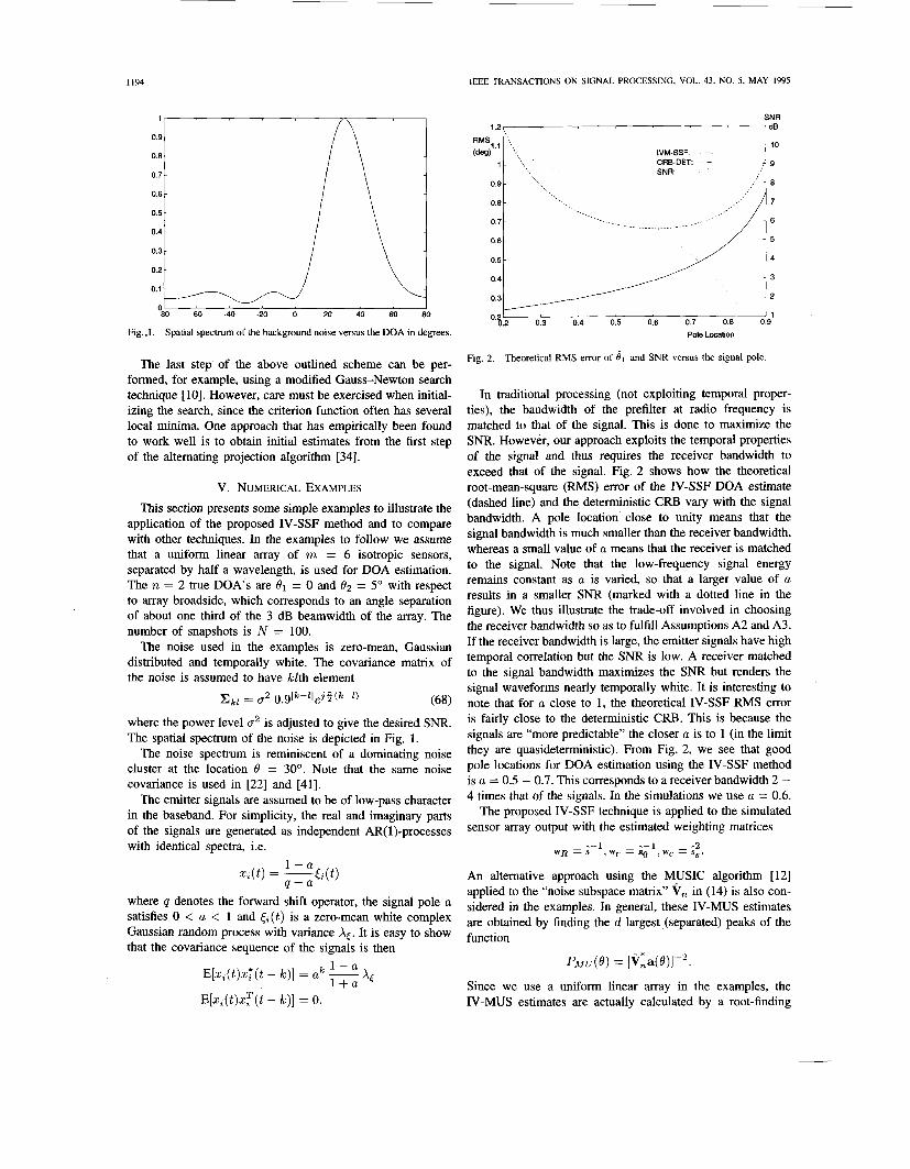
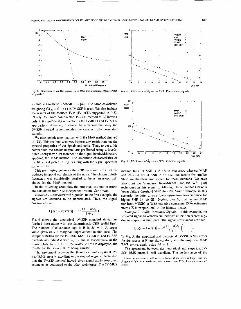
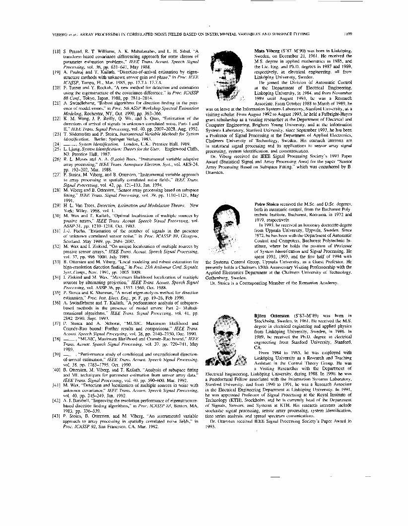
Fig. .l. Spatial spectrum of the background noise versus the DOA in degrees.

The last step of the above outlined scheme can be per- formed, for example, using a modified Gauss-Newton search technique [lo]. However, care must be exercised when initial- izing the search, since the criterion function often has several local minima. One approach that has empirically been found to work well is to obtain initial estimates from the first step of the alternating projection algorithm [34].

V. NUMERICAL EXAMPLES This section presents some simple examples to illustrate the

application of the proposed IV-SSF method and to compare with other techniques. In the examples to follow we assume that a uniform linear array of m = 6 isotropic sensors, separated by half a wavelength, is used for DOA estimation. The n = 2 true D0A”s are 61 = 0 and 62 = 5” with respect to array broadside, which corresponds to an angle separation of about one third of the 3 dB beamwidth of the array. The number of snapshots is N = 100.

The noise used in the examples is zero-mean, Gaussian distributed and temporally white. The covariance matrix of the noise is assumed to have klth element

Ekl = (J2 O.glk-llej%(k-l) (68) where the power level o2 is adjusted to give the desired SNR. The spatial spectrum of the noise is depicted in Fig. 1.

The noise spectrum is reminiscent of a dominating noise cluster at the location 6 = 30”. Note that the same noise covariance is used in [22] and [41].

The emitter signals are assumed to be of low-pass character in the baseband. For simplicity, the real and imaginary parts of the signals are generated as independent AR( 1)-processes with identical spectra, i.e.

where q denotes the forward shift operator, the signal pole a satisfies 0 < a < 1 and &(t) is a zero-mean white complex Gaussian random process with variance A t . It is easy to show that the covariance sequence of the signals is then

1 - a I t a

E [ ~ i ( t ) ~ ; ( t - k)] = ak - A t

E[X;(t)xT(t - k)] = 0.

IVM-SSF: - ~ - - - CRB-DET: - SNR:

,,:‘ 8

Pole Location

Fig. 2. Theoretical RMS error of 81 and SNR versus the signal pole.

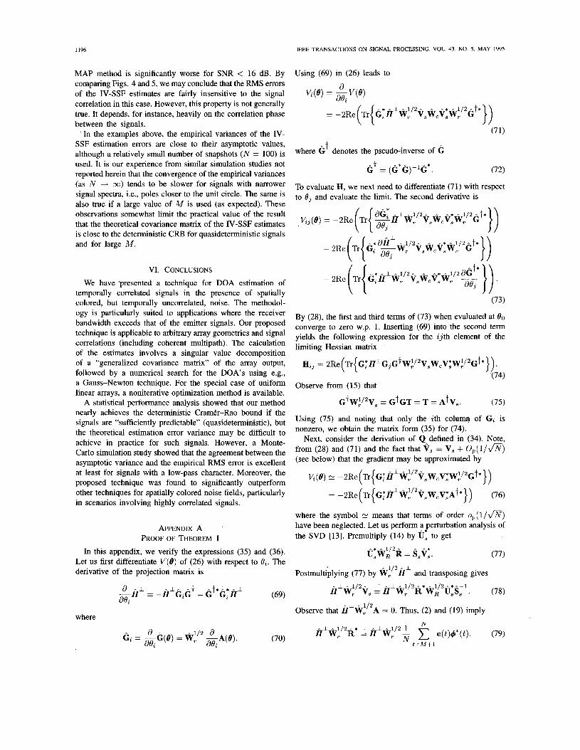
In traditional processing (not exploiting temporal proper- ties), the bandwidth of the prefilter at radio frequency is matched to that of the signal. This is done to maximize the SNR. However, our approach exploits the temporal properties of the signal and thus requires the receiver bandwidth to exceed that of the signal. Fig. 2 shows how the theoretical root-mean-square (RMS) error of the IV-SSF DOA estimate (dashed line) and the deterministic CRB vary with the signal bandwidth. A pole location close to unity means that the signal bandwidth is much smaller than the receiver bandwidth, whereas a small value of a means that the receiver is matched to the signal. Note that the low-frequency signal energy remains constant as a is varied, so that a larger value of a results in a smaller SNR (marked with a dotted line in the figure). We thus illustrate the trade-off involved in choosing the receiver bandwidth so as to fulfill Assumptions A2 and A3. If the receiver bandwidth is large, the emitter signals have high temporal correlation but the SNR is low. A receiver matched to the signal bandwidth maximizes the SNR but renders the signal waveforms nearly temporally white. It is interesting to note that for a close to 1, the theoretical N-SSF RMS error is fairly close to the deterministic CRB. This is because the signals are “more predictable” the closer a is to 1 (in the limit they are quasideterministic). From Fig. 2, we see that good pole locations for DOA estimation using the IV-SSF method is a = 0.5 - 0.7. This corresponds to a receiver bandwidth 2 - 4 times that of the signals. In the simulations we use a = 0.6.

The proposed IV-SSF technique is applied to the simulated sensor array output with the estimated weighting matrices

A- 1 - -1 -2 W R = S , W r = R g , W c = S S’

An alternative approach using the MUSIC algorithm [12] applied to the “noise subspace matrix” V, in (14) is also con- sidered in the examples. In general, these IV-MUS estimates are obtained by finding the d largest (separated) peaks of the function

P M U ( 0 ) = lV;a(e)l-2.

Since we use a uniform linear array in the examples, the IV-MUS estimates are actually calculated by a root-finding

VIBERG et al.: ARRAY PROCESSING IN CORRELATED NOISE FIELDS BASED ON INSTRUMENTAL VARIABLES AND SUBSPACE FITTING 1195

Filter: - - - - - Signal: -

dB

-4 - 1

-5 -

-6 -

Filter: - - - - - Signal: -

dB

-4 - 1

-5 -

-6 -

10'

RMS (de@

-9

-loo 0:l 0:2 0:3 0:4 '0:5 0:6 0:7 0:8 0:9 1

Normalized Frequency

IV-RED: + I . MAP: o

IV-MUS: * IV-SSF: x ....... CRB-DET ~

+ +

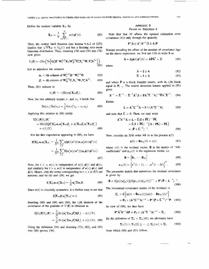
Fig, 3. of prefilter.

Spectrum of emitter signals (a = 0.6) and amplitude characteristic

+=

technique similar to Root-MUSIC [42]. The same covariance weighting (WE = S-l) as in IV-SSF is used. We also include the results of the reduced IVM (IV-RED) suggested in [43]. Clearly, the more complicated IV-SSF method is of interest only if it significantly outperforms the IV-RED and IV-MUS approaches. However, it should be remarked that only the IV-SSF method accommodates the case of fully correlated signals.

We also include a comparison with the MAP method derived in [22]. This method does not impose any restrictions on the spectral properties of the signals and noise. Thus, to get a fair comparison the sensor outputs are prefiltered using a fourth- order Chebyshev filter matched to the signal bandwidth before applying the MAP method. The amplitude characteristics of the filter is depicted in Fig. 3 along with the signal spectrum for a = 0.6.

This prefiltering enhances the SNR by about 3 dB, but in- troduces temporal correlation of the noise. The chosen cutoff- frequency was empirically verified to be a "near-optimal" choice for the MAP method.

In the following examples, the empirical estimation errors are calculated from 512 independent Monte Carlo runs.

Example I-Uncorrelated Signals: In the first example, the signals are assumed to be uncorrelated. Thus, the signal covariances are

I. k (1 - a)% E[x( t - k)x* ( t ) ] = a l + a

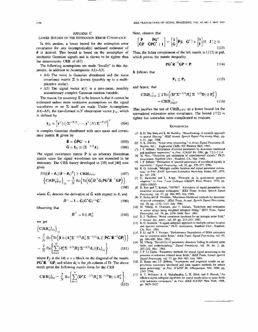
Fig. 4 shows the theoretical IV-SSF standard deviations (dashed line) along with the deterministic CRB (solid line). The number of covariance lags in R is M = 1. A larger value gives only a marginal improvement in this case. The sample statistics for the IV-RED, MAP, IV-MUS, and IV-SSF methods are indicated with +, 0, * and 2, respectively, in the figure. Only the results for the source at 0' are displayed, the results for the source at 5" being similar.

The agreement between the theoretical and empirical IV- SSF RMS error is excellent in the studied scenario. Note also that the IV-SSF method indeed gives significantly improved estimates as compared to the other techniques. The IV-MUS

0 , -._,

..-... x

4 6 8 10 12 14 16 16 20 22 24 1 0 '

SNR (dB)

Fig. 4. RMS error of 6, versus SNR. Uncorrelated signals.

loo>-, .4.. 1 -.. ..- x... ... --. %...

..__ ...

-...x.-

4 6 8 10 12 14 16 18 20 22 24 lo - '

SNR (dB)

Fig. 5. RMS error of 81 versus SNR. Coherent signals.

method fails3 at SNR < 8 dB in this case, whereas MAP and IV-RED fail at SNR < 16 dB. The results for smaller SNR are therefore not shown for these methods. We have also tried the "standard" Root-MUSIC and the WSF [lo] techniques in this scenario. Although these methods have a lower failure threshold SNR than the MAP technique in this scenario, the latter gives a lower estimation error variance for higher SNR (> 16 dB). Notice, though, that neither MAP nor Root-MUSIC or WSF can give consistent DOA estimates unless C is proportional to the identity matrix.

Example 2-Fully Correlated Signals: In this example, the received signal waveforms are identical at the first sensor, e.g., due to a specular multipath. The signal covariances are then

E[x(t - k)x*(t)] = ak

In Fig. 5 , the empirical and theoretical IV-SSF RMS errors for the source at 0' are shown along with the empirical MAP RMS errors, again using M = 1 .

The agreement between the theoretical and empirical IV- SSF RMS errors is still excellent. The performance of the

3Here, an estimate is said to be a failure if the error is larger than 5'. A method fails in a certain scenario if more than 30% of the estimates are failures.

1196 IEEE TRANSACTIONS ON SIGNAL PROCESSING, VOL. 43, NO. 5, MAY 1995

MAP method is significantly worse for SNR < 16 dB. By comparing Figs. 4 and 5, we may conclude that the RMS errors of the IV-SSF estimates are fairly insensitive to the signal correlation in this case. However, this property is not generally true. It depends, for instance, heavily on the correlation phase between the signals. . In the examples above, the empirical variances of the IV-

SSF estimation errors are close to their asymptotic values, although a relatively small number of snapshots (N = 100) is used. It is our experience from similar simulation studies not reported herein that the convergence of the empirical variances (as N + 00) tends to be slower for signals with narrower signal spectra, i.e., poles closer to the unit circle. The same is also true if a large value of M is used (as expected). These observations somewhat limit the practical value of the result that the theoretical covariance matrix of the IV-SSF estimates is close to the deterministic CRJ3 for quasideterministic signals and for large M.

VI. CONCLUSIONS

We have ’presented a technique for DOA estimation of temporally correlated signals in the presence of spatially colored, but temporally uncorrelated, noise. The methodol- ogy is particularly suited to applications where the receiver bandwidth exceeds that of the emitter signals. Our proposed technique is applicable to arbitrary array geometries and signal correlations (including coherent multipath). The calculation of the estimates involves a singular value decomposition of a “generalized covariance matrix” of the array output, followed by a numerical search for the DOA’s using e.g., a Gauss-Newton technique. For the special case of uniform linear arrays, a noniterative optimization method is available.

A statistical performance ana€ysis showed that our method nearly achieves the deterministic Cramer-Rao bound if the signals are “sufficiently predictable” (quasideterministic), but the theoretical estimation error variance may be difficult to achieve in practice for such signals. However, a Monte- Carlo simulation study showed that the agreement between the asymptotic variance and the empirical RMS error is excellent at least for signals with a low-pass character. Moreover, the proposed technique was found to significantly outperform other techniques for spatially colored noise fields, particularly in scenarios involving highly correlated signals.

APPENDIX A PROOF OF THEOREM 1

In this appendix, we verify the expressions (35) and (36). Let us first differentiate V(@) of (26) with respect to Oi. The derivative of the projection matrix is

where

Using (69) in (26) leads to

..* - I A 1/2- A * n 1/2- t* Gi17 W, V,W,V,W, G

- t where G denotes the pseudo-inverse of G

(72)

To evaluate H, we next need to differentiate (71) with respect to Oj and evaluate the limit. The second derivative is

e t = (G*G)-lG*.

(73)

By (28), the first and third terms of (73) when evaluated at 80 converge to zero w.p. 1. Inserting (69) into the second term yields the following expression for the ij.th element of the limiting Hessian matrix

H,, = 2Re(Tr{ G:17LG,CtW:/2V,W,V:W:/2Gt*}). (74)

(75)

Using (75) and noting that only the ith column of G, is nonzero, we obtain the matrix form (35) for (74).

Next, consider the derivation of Qadefined in (34). Note, from (28) and (71) and the fact that V, = V, + 0 , ( 1 / 0 ) (see below) that the gradient may be approximated by

Observe from (15) that

G ~ w : / ~ v , = G ~ G T = T = A ~ v , .

&(e) N -2Re(Tr{G:17 I W, 1/2 V,W,V:W~/2Gt*}) ..

= -2Re(Tr{ G:fiLW~/2V,W,V:At*}) (76)

where the symbol N means that terms of order o P ( 1 / 0 ) have been neglected. Let us perform !+perturbation analysis of the SVD [13]. Premultiply (14) by U, to get

(77) .. * .. 1/2 U,W, R = SsVs.

..*

.. 1/2 I Postmulti’plying (77) by W, 17 and transposing gives

A I .. 1/2 .. 17 W, V, =17 W, R W, U,S, . (78)

-1 .. 1 /2 -* .. 1/2-*--1

.. I A 1/2 Observe that 17 W, A = 0. Thus, (2) and (19) imply

- 1 - 1 / 2 - * A1A1/21 N

17 W, R = 17 W, - e( t )d*(t) . (79) t=M+l (70)

- a 1/2 d - doi 80;

G . - -G(@) = W, -A(@).

1 I97 VIBERG et al.: ARRAY PROCESSING IN CORRELATED NOISE FIELDS BASED ON INSTRUMENTAL VARIABLES AND SUBSPACE FITTING

Define the random variable XN by

- N

Then, the central limit theorem (see lemma 9.A.2 of [25]) implies that ~ X N is O,(l) and has a limiting zero-mean Gaussian distribution. Thus, inserting (78) and (79) into (76) now gives

K(6) ? -2Re(Tr{ G~II'wf./2X~w~2u:s;1w,v~t*}). (81)

(829

(83)

Let us introduce the notation

a, = ith column of w ~ / ~ I I ~ w ~ / ~ D

/?, = ith column of Wi'2UsS;'W,V:At*.

Then, (81) reduces to

K(0) _N -2Re(a:X~&). (84)

Now, for two arbitrary scalars 2 1 and 2 2 , it holds that

(85) 1

Re(z1) Re(22) = -Re(xTz, + z1 Q). 2

Applying this relation to (84) yields

E[K (e)v, (611 = 2Re(E[P:X>aza,*X~P, + c r : X ~ P , a j x ~ P , ] )

+ o ( l / N ) . (86)

For the first expectation appearing in (86), we have

1 E [ X k a i a j * X ~ ] = 7 E[4(t)e*(t)azaj*e(s)4*(s)]

t , s

1 = - E[orj*e(s)e*(t)ai4(t)4*(s)].

N 2 t .s

(87)

Now, for t < s, e(s) is independent of e ( t ) , d ( t ) and 4(s), and similarly for t > s, e( t ) is independent of e(s),4(s) and 4(t). Hence, only the terms corresponding to t = s in (87) are nonzero, and by (6) and (39), we get

(88)

Since e ( t ) is circularly symmetric, it is further easy to see that

1 N

E [ X k a , a j X ~ ] = -a,'&,S.

E [ X N @ , ~ ~ X N ] = 0. (89)

Inserting (88) and (89) into (86), the ijth element of the covariance of the gradient of V(6) is obtained as

2 E[K(6)V,(6)1 = -Re(~,*~a,/?:S/?J N + o ( l / N )

n

= kRe(a:EaJ/?;S/? , ) + o ( l / N ) . (90)

Using the definition (34) and inserting ( 7 3 , (82), and (83) into (90) proves (36).

N

APPENDIX B PROOF OF THEOREM 4

Note first that M affects the optimal estimation error covariance (41) only through the quantity

P*(I 8 A*)S-l(I 8 A)P.

Toward revealing the effect of the number of covariance lags on the above expression, we first use (10) to write S as

S = E[#(t)q5*(t)] = APA* + % (91)

where

A = I @ A (92) C = I @ E (93)

and where P is a block Toeplitz matrix, with its ijth block equal to Pi-j. The matrix inversion lemma applied to (91) gives

(94) s-1 - - 2-1 - %-1A*(I + p A * p A ) - l p A * % - l .

Define

L = A * % - ~ A = I g ( A * E - ~ A ) (95)

and note that L > 0. Then, we may write

A*s-lA = L - L(I + PL)-lPL = L(I + PL)-l{ (I + PL) - PL}

= (P + L - y . (96)

Now, consider an Mth order AR fit to the process z ( t )

~ ( t ) - B z M ( ~ ) = ~ ( t ) (97)

where E ( t ) is the residual vector, B is the matrix of "AR- coefficients" and znl(t) is the regression vector, i.e.

B = [ B ~ , . . . , B M ] (98) T

Z A l ( t ) = [zT(t - l ) , . . . , zT( t - M ) ] . (99)

The parameter matrix that minimizes the residual covariance is given by

- - 1 -1 B = E [ ~ ( t ) z > ( t ) ] ( E [ z ~ ( t ) ~ > ( t ) ] ) - ' = P*(P + L ) . (100)

The minimized covariance matrix of the residuals is

C, = E[(z(t) - BzM(t ) ) ( z ( t ) - B z ~ ( t ) ) * ]

= p0 + ( A * E - ~ A ) - ~ - P*(P + L-l)- lp. (101)

In view of (96), we thus have

By the definition of EE = E,(M), we obviously have

E:E(l) 2 EE(2) 2 . . . 2 E E ( w ) = Ee (103)

from which (60) and (61) follow.

1198 IEEE TRANSACTlONS ON SIGNAL PROCESSING, VOL. 43, NO. 5, MAY 1995

APPENDIX C LOWER BOUNDS ON THE ESTIMATION ERROR COVARIANCE

In this section, a lower bound for the estimation error covariance for any (asymptotically) unbiased estimator of 0 is derived. This bound is based on the assumption of stochastic Gaussian signals and is shown to be tighter than the deterministic CRB of (67).

The following assumptions are made “locally” in this Ap- pendix, in addition to Assumptions Al)-A3).

A4) The noise is Gaussian distributed and the noise is known (possibly up to a multi-

A5) The signal vector x(t) is a zero-mean, possibly

The reason for assuming X to be known is that it cannot be estimated unless more restrictive assumptions on the signal waveforms or on X itself are made. Under Assumptions Al)-A5), the transformed mN observation vector yN, which is defined by

covariance matrix plicative scalar).

nonstationary complex Gaussian random variable.

y N = y T ( 1) X-T/2 , . . . , y T ( N ) X - T / 2 ] (104)

is complex Gaussian distributed with zero mean and covari- ance matrix R given by

[

R = GPG* + I G = IN ’@ (E-’”A).

(105) (106)

The signal covariance matrix P is an arbitrary Hermitean matrix since the signal waveforms are not restricted to be stationary. The CRB theory developed in [39] and [40] now gives

N E [ ( B - B ~ ) ( ~ - ~ ~ ) ~ ] 2 C R B ~ ~ ~ (107) { CRBi;o}zj = 2 Re{ Tr(G,*@G,PG * - - I - - R GP)} N

(108)

where G i denotes the derivative of G with respect to Oi and

(109) f-p = 1 - G(G*G)-IG*.

Observing that

nl = I @ @ (1 10)

we get

= 4 Re{Tr([I @ (ArX-1/217iC-1/2A;)] [PG*R-’GP])} N

= - Re C(d5X-’/2~iC-’izdi){Fk}ij N

N {k=l

where Fk is the kth n x n block on the diagonal of the matrix PG’R-lGP, and where di is the j th column of D. The above result gives the following matrix form for the CRB

Next, observe that

(113) [;I [GP P GE* PG* + I ] = [;]Pp e*]+ [O I ] 2 0.

Thus, the Schur complement of the left matrix in (1 13) is psd, which proves the matrix inequality

E ’ R - l G P 5 P. (1 14)

It follows that

and hence, that

CRBi$o 5 2Re{ (D*X-1/zllkX-1/2D) 0 P,T)

= CRB& (1 16)

This justifies the use of CRBDET as a lower bound for the normalized estimation error covariance. The bound (1 12) is tighter but somewhat more complicated to evaluate.

REFERENCES

[ I ] B. D. Van Veen and K. M. Buckley, “Beamforming: A versatile approach to spatial filtering,” IEEE Acoust. Speech Signal Processing Mag., pp. 4-24, Apr. 1988.

[2] N. L. Owsley, “Sonar array processing,” in Array Signal Processing (S. Haykin, Ed.).

[3] J. F. Bohme, “Estimation of source parameters by maximum likelihood and nonlinear regression,” in Proc. ICASSP 84, 1984, pp. 7.3.1-7.3.4.

[4] M. Wax, “Detection and estimation of superimposed signals,’’ Ph.D. dissertation, Stanford Univ., Stanford, CA, Mar. 1985.

[5] J. F. Bohme, “Estimation of spectral parameters of correlated signals in wavefields,” Signal Processing, vol. 10, pp. 329-337, 1986.

[6] R. 0. Schmidt, “Multiple emitter location and signal parameter estima- tion,” in Proc. RADC Spectrum Estimation Workshop, Rome, NY, 1979, pp. 243-258.

[7] G. Bienvenu and L. Kopp, “Principle de la goniometrie passive adaptive,” in Proc. 7’eme Colloque GRESIT, Nice, France, 1979, pp.

[8] R. Roy and T. Kailath, “ESPRIT-Estimation of signal parameters via rotational invariance techniques,” IEEE Trans. Acoust. Speech Signal Processing, vol. 37, pp. 984-995, July 1989.

[9] P. Stoica and K. Sharman, “Maximum likelihood methods for direction- of-arrival estimation,” IEEE Trans. Acoust. Speech Signal Processing,

[lo] M. Viberg, B. Ottersten, and T. Kailath, “Detection and estimation in sensor arrays using weighted subspace fitting,” IEEE Trans. Signal Processing, vol. 39, pp. 2436-2449, Nov. 1991.

[ 111 R. J. Thalham, “Noise correlation functions for an isotropic noise field,” J. Acoust. Soc. Amer., vol. 69, pp. 213-215, 1981.

[12] R. 0. Schmidt, “A signal subspace approach to multiple emitter location and spectral estimation,” Ph.D. dissertation, Stanford Univ., Stanford, CA, Nov. 1981.

[13] F. Li and R. J. Vaccaro, “Performance Degradation of DOA estimators due to unknown noise fields,” IEEE Trans. Signal Processing, vol. 40, pp. 686689, Mar. 1992.

[I41 M. Viberg, “Sensitivity of parametric direction finding to colored noise fields and undermodeling,” Signal Processing, vol. 34, no. 2, pp.

[I51 J. P. Le Cadre, “Parametric methods for spatial signal processing in the presence of unknown colored noise fields,” IEEE Trans. Acoust. Speech Signal Processing, vol. 37, pp. 965-983, July 1989.

[I61 D. Kraus and J.F. Bohme, “Asymptotic and empirical results on ap- proximate maximum likelihood and least squares methods for sensor array processing,” in Proc. lCASSP 90, Albuquerque, Nh4, 1990, pp. 2795-2798.

[I71 R. T. Williams, A. K. Mahalanabis, L. H. Sibul, and S. Prasad, “An efficient signal subspace algorithm for source localization in noise fields with unknown covariance,” in Proc. IEEE ICASSP, New York, 1988, pp. 2829-2832.

Englewood Cliffs, NJ: Prentice Hall, 1985.

1061 1-106/10.

vol. 38, pp. 1132-1143, July 1990.

207-222, NOV. 1993.

VIBERG et al.: ARRAY PROCESSING IN CORRELATED NOISE FIELDS BASED ON INSTRUMENTAL VARIABLES AND SUBSPACE FITTING 1199

S. Prasad, R. T. Williams, A. K. Mahalanahis, and L. H. Sibul, “A transform-based covariance differencing approach for some classes of parameter estimation problems,” IEEE Trans. Acoust. Speech Signal Processing, vol. 36, pp. 631-641, May 1988. A. Paulraj and T. Kailath, “Direction-of-arrival estimation by eigen- structure methods with unknown sensor gain and phase,” in Proc. IEEE ICASSP, Tampa, FL, Mar. 1985, pp. 17.7.1-17.7.4. F. Tuteur and Y, Rockab, “A new method for detection and estimation using the eigenstructure of the covariance difference,” in Proc. ICASSP 88 Con$, Tokyo, Japan, 1988, pp. 2811-2814. A. Swindlehurst, “Robust algorithms for direction-finding in the pres- ence of model errors,” in Proc. 5th ASSP Workshop Spectral Estimation Modeling, Rochester, NY, Oct. 1990, pp. 362-366. K. M. Wong, J. P. Reilly, Q. Wu, and S. Qiao, “Estimation of the directions of arrival of signals in unknown correlated noise, Parts I and 11,” IEEE Trans. Signal Processing, vol. 40, pp. 2007-2028, Aug. 1992. T. Soderstrom and P. Stoica, Instrumental Variable Methods for System Identification. Berlin: Springer-Verlag, 1983. __, System Identijkation. L. Ljung, System Identification: Theory for the User. Englewood Cliffs, NJ: Prentice Hall, 1987. R. L. Moses and A. A. (Luois) Beex, “Instrumental variable adaptive array processing,” IEEE Trans. Aerospace Electron. Syst., vol. AES-24, pp. 192-202, Mar. 1988. P. Stoica, M. Viherg, and B. Ottersten, “Instrumental variable approach to array processing in spatially correlated noise fields,” IEEE Trans. Signal Processing, vol. 42, pp. 121-133, Jan. 1994. M. Viberg and B. Ottersten, ‘Sensor array processing based on subspace fitting,” IEEE Trans. Signal Processing, vol. 39, pp. 1 1 10-1 121, May 1991. H. L. Van Trees, Detection, Estimation and Modulation Theory. New York: Wiley, 1968, vol. I . M. Wax and T. Kailath, “Optimal localization of multiple sources by passive arrays,’’ IEEE Trans. Acoust. Speech Signal Processing, vol. ASSP-31, pp. 1210-1218, Oct. 1983. J.-J. Fuchs, “Estimation of the number of signals in the presence of unknown correlated sensor noise,” in Proc. ICASSP 89, Glasgow, Scotland, May 1989, pp. 2684-2687. M. Wax and I. Ziskind, “On unique localization of multiple sources by passive sensor arrays,” IEEE Trans. Acoust. Speech Signal Processing, vol. 37, pp. 9961000, July 1989. B. Ottersten and M. Viberg, “Local modeling and robust estimation for high-resolution direction finding,” in Proc. 25th Asilomar Conf Signals, Syst., Comp., Nov. 1 99 1, pp. 1005-1 009. I. Ziskind and M. Wax, “Maximum likelihood localization of multiple sources by alternating projection,” IEEE Trans. Acoust. Speech Signal Processing, vol. ASSP-36, pp. 1553-1560, Oct. 1988. P. Stoica and K. Sharman, “A novel eigenanalysis method for direction estimation,” Proc. Inst. Elect. Eng.. pt. F, pp. 19-26, Feh 1990. A. Swindlehurst and T. Kailath, “A performance analysis of subspace- based methods in the presence of model errors: Part 2-Multidi- mensional algorithms,” IEEE Trans. Signal Processing, vol. 41, pp. 2882-2890, Sept. 1993. P. Stoica and A. Nehorai, “MUSIC, Maximum likelihood and CramCr-Rao bound: Further results and comparisons,” IEEE Trans. Acousr. Speech Signal Processing, vol. 38, pp. 2140-2150, Dec. 1990. __, “MUSIC, Maximum likelihood and Cramtr-Rao bound,” IEEE Trans. Acoust. Speech Signal Processing, vol. 37, pp. 720-741, May 1989. __ , “Performance study of conditional and unconditional direction- of-arrival estimation,” IEEE Trans. Acoust. Speech Signal Processing, vol. 38, pp. 1783-1795, Oct. 1990. B. Ottersten, M. Viberg, and T. Kailath, “Analysis of subspace fitting and ML techniques for parameter estimation from sensor array data,” IEEE Trans. Signal Processing, vol. 40, pp. 5 9 W 0 , Mar. 1992. M. Wax, “Detection and localization of multiple sources in noise with unknown covariance,” IEEE Trans. Acoust. Speech Signal Processing, vol. 40, pp. 245-249, Jan. 1992. A. J. Barabell, “Improving the resolution performance of eigenstructure- based direction-finding algorithms,” in Proc. ICASSP 83, Boston, MA, 1983, pp. 336339. P. Stoica, B. Ottersten, and M. Viberg, “An instrumental variable approach to array processing in spatially correlated noise fields,” in Proc. ICASSP 92, San Francisco, CA, Mar. 1992.

London, U.K.: Prentice Hall, 1989.

Mats Viberg (S’87-M’90) was horn in Linkoping, Sweden, on December 21, 1961. He received the M S degree in applied mathematics in 1985, and the Lic. Eng. and Ph.D. degrees in 1987 and 1989, respectively, in elecmcal engineering, all from Linkoping University, Sweden

He joined the Division of Automatic Control at the Department of Electncal Engineenng, Linkoping University, in 1984, and from November 1989 until August 1993, be was a Research Associate. From October 1988 to March of 1989, he

was on leave at the Information Systems Laboratory, Stanford University, as a visiting scholar. From August 1992 to August 1993, he held a Fulbnght-Hayes grant scholarship as a visiting researcher at the Department of Elecmcal and Computer Engineenng, Bngham Young University, and at the Informabon Systems Laboratory, Stanford University. since September 1993, he has been a Professor of Signal Processing at the Department of Applied Electronics, Chalmers University of Technology, Sweden. His research interests are in statistical signal processing and its applications to sensor array signal processing, system identification, and communication.

Dr. Viherg received the IEEE Signal Processing Society’s 1993 Paper Award (Statistical Signal and Array Processing Area) for the paper “Sensor Array Processing Based on Subspace Fitting,” which was coauthored by B. Ottersten.

Petre Stoica received the M Sc. and D.Sc. degrees, both in automatic control, from the Bucharest Poly- technic Institute, Bucharest, Romania, in 1972 and 1979, respectively.

In 1993, he received an honorary doctorate degree from Uppsala University, Uppsala, Sweden. Since 1972, he has been with the Department of Automatic Control and Computers, Bucharest Polytechnic In- stitute, where he holds the position of Professor of System Identification and Signal Processing. He spent 1992, 1993, and the first half of 1994 with

the Systems Control Group, Uppsala University, as a Guest Professor. He presently holds a Chalmers 150th Anniversary Visiting Professorship with the Applied Electronics Department at the Chalmers University of Technology, Gothenhurg, Sweden.

Dr. Stoica is a Corresponding Member of the Romanian Academy.

Bjorn Ottersten (S’87-M’89) was horn in Stockholm, Sweden, in 1961. He received the M.S. degree in electrical enginering and applied physics from Linkoping University, Sweden, in 1986. In 1989, he received the Ph.D. degree in electrical engineering from Stanford University, Stanford, CA.

From 1984 to 1985, he was employed with Linkoping University as a Research and Teaching Assistant in the Control Theory Group. He was a Visiting Researcher with the Department of

Electrical Engineering, Linkoping University, during 1988. In 1990, he was a Postdoctural Fellow associated with the Information Systems Laboratory, Stanford University, and from 1990 to 1991, he was a Research Associate in the Electrical Engineering Department at Linkoping University. In 1991, he was appointed Professor of Signal Processing at the Royal Institute of Technology (KTH), Stockholm, and he is currently head of the Department of Signals, Sensors, and Systems at KTH. His research interests include stochastic signal processing, sensor array processing, system identification, time series analysis, and spread spectrum comunications.

Dr. Ottersten received IEEE Signal Processing Society’s Paper Award in 1993.