Instrumental Uncertainties in Z–R Relations
15
1088 VOLUME 39 JOURNAL OF APPLIED METEOROLOGY q 2000 American Meteorological Society Instrumental Uncertainties in Z–R Relations EDWIN CAMPOS* AND ISZTAR ZAWADZKI Department of Atmospheric and Oceanic Sciences, McGill University, Montreal, Quebec, Canada (Manuscript received 17 December 1998, in final form 21 June 1999) ABSTRACT Intercomparisons among three different sensors for ground-based measurement of drop size distributions are presented: the Joss–Waldvogel distrometer, the optical spectro-pluviometer, and the precipitation occurrence sensor system. Data corresponding to stratiform, continental rain are analyzed, and reflectivity factor–rain rate at the ground (Z–R) relationships are obtained from simultaneous measurements by the three sensors. The Z–R relations derived from the three sensors show differences comparable to the ones seen in distinct climatic regions. In addition, the Z–R relationships are found to be sensitive to the data analysis method. 1. Introduction Remote sensing measurements of rain by radars are based on the relationship between reflectivity factor Z and rain rate at the ground R. This relation can be ob- tained either through a theoretical or an empirical ap- proach. Marshall and Palmer (1948) demonstrated the existence of a drop size distribution (DSD) that is a simple function of R, leading to a simple relation be- tween Z and R. Since then, many relationships were proposed, depending on geographical location and phys- ical conditions of the precipitation. In addition, radar rainfall quantification is affected by many practical lim- itations, especially at longer ranges (Zawadzki 1984). At ranges shorter than 80 km, however, the accuracy of radar measurements is limited mainly by the variability of drop size distributions as long as the radar detection is below bright band. Empirical relations of the form Z 5 aR b are used, with R and Z obtained from DSD mea- surements. DSD is a function that expresses the number N of drops per unit size interval (usually diameter D ) and per unit volume of space [i.e., N(D ), (m 23 mm 21 )]. The variability of DSDs with kind of precipitation and its influence on the Z–R relationship appears to be, even after many years of studies, a subject of unexhausted interest. When averages of long-term observations (sev- * Current affiliation: Instituto Meteorolo ´gico Nacional, San Jose ´, Costa Rica. Corresponding author address: Isztar Zawadzki, Dept. of Atmo- spheric and Oceanic Sciences, McGill University, 805 Sherbrooke St. W., Montreal, PQ H3A 2K6, Canada. E-mail: [email protected] eral hours of data) are taken, DSDs are very stable and follow the exponential distribution, very similar to the one proposed by Marshall and Palmer (1948). Three types of DSDs, convective, stratiform, and drizzle, usu- ally are distinguished. Storm-to-storm variability, changes during the life cycle of a precipitation system, and regional variability are some of the questions not yet definitely resolved, however. These issues are cloud- ed by the uncertainty concerning the influence of in- strument sampling volume, instrumental shortcomings, and the method of data processing on the reported ob- servations. Radar samples a volume on the order of 1 km 3 . How does DSD within such a volume relate to small samples such as aircraft measurements along a line or ground-based distrometric measurements? Are the instruments stable enough so that the observed sam- ple-to-sample variability can be attributed to nature and not to differences among the instruments or drifts in instrumental performance? Do the different instruments respond to the different precipitation kinds in the same manner? These are some relevant questions that have received little attention. Thus, it is necessary to examine the behavior of the instruments to get a feeling for what distrometric in- formation is trustworthy. Since the ‘‘true DSD’’ is not known, the only way of getting an insight into the in- strumental limitations is by intercomparison of individ- ual samples and averages given by different instruments. The most widely used of these instruments is the distrometer developed by Joss and Waldvogel (1967)— to be called JWD. Optical devices [such as the optical spectro-pluviometer, (OSP) described in Hauser et al. (1984)] as well as radar measurements of Doppler ve- locity spectrum [as in the precipitation occurrence sen- sor system (POSS) described in Sheppard (1990b)] have
Transcript of Instrumental Uncertainties in Z–R Relations
1088 VOLUME 39J O U R N A L O F A P P L I E D M E T E O R O L O G Y
q 2000 American Meteorological Society
Instrumental Uncertainties in Z–R Relations
EDWIN CAMPOS* AND ISZTAR ZAWADZKI
Department of Atmospheric and Oceanic Sciences, McGill University, Montreal, Quebec, Canada
(Manuscript received 17 December 1998, in final form 21 June 1999)
ABSTRACT
Intercomparisons among three different sensors for ground-based measurement of drop size distributions arepresented: the Joss–Waldvogel distrometer, the optical spectro-pluviometer, and the precipitation occurrencesensor system. Data corresponding to stratiform, continental rain are analyzed, and reflectivity factor–rain rateat the ground (Z–R) relationships are obtained from simultaneous measurements by the three sensors. The Z–Rrelations derived from the three sensors show differences comparable to the ones seen in distinct climatic regions.In addition, the Z–R relationships are found to be sensitive to the data analysis method.
1. Introduction
Remote sensing measurements of rain by radars arebased on the relationship between reflectivity factor Zand rain rate at the ground R. This relation can be ob-tained either through a theoretical or an empirical ap-proach. Marshall and Palmer (1948) demonstrated theexistence of a drop size distribution (DSD) that is asimple function of R, leading to a simple relation be-tween Z and R. Since then, many relationships wereproposed, depending on geographical location and phys-ical conditions of the precipitation. In addition, radarrainfall quantification is affected by many practical lim-itations, especially at longer ranges (Zawadzki 1984).At ranges shorter than 80 km, however, the accuracy ofradar measurements is limited mainly by the variabilityof drop size distributions as long as the radar detectionis below bright band. Empirical relations of the form Z5 aRb are used, with R and Z obtained from DSD mea-surements.
DSD is a function that expresses the number N ofdrops per unit size interval (usually diameter D) andper unit volume of space [i.e., N(D), (m23 mm21)]. Thevariability of DSDs with kind of precipitation and itsinfluence on the Z–R relationship appears to be, evenafter many years of studies, a subject of unexhaustedinterest. When averages of long-term observations (sev-
* Current affiliation: Instituto Meteorologico Nacional, San Jose,Costa Rica.
Corresponding author address: Isztar Zawadzki, Dept. of Atmo-spheric and Oceanic Sciences, McGill University, 805 SherbrookeSt. W., Montreal, PQ H3A 2K6, Canada.E-mail: [email protected]
eral hours of data) are taken, DSDs are very stable andfollow the exponential distribution, very similar to theone proposed by Marshall and Palmer (1948). Threetypes of DSDs, convective, stratiform, and drizzle, usu-ally are distinguished. Storm-to-storm variability,changes during the life cycle of a precipitation system,and regional variability are some of the questions notyet definitely resolved, however. These issues are cloud-ed by the uncertainty concerning the influence of in-strument sampling volume, instrumental shortcomings,and the method of data processing on the reported ob-servations. Radar samples a volume on the order of 1km3. How does DSD within such a volume relate tosmall samples such as aircraft measurements along aline or ground-based distrometric measurements? Arethe instruments stable enough so that the observed sam-ple-to-sample variability can be attributed to nature andnot to differences among the instruments or drifts ininstrumental performance? Do the different instrumentsrespond to the different precipitation kinds in the samemanner? These are some relevant questions that havereceived little attention.
Thus, it is necessary to examine the behavior of theinstruments to get a feeling for what distrometric in-formation is trustworthy. Since the ‘‘true DSD’’ is notknown, the only way of getting an insight into the in-strumental limitations is by intercomparison of individ-ual samples and averages given by different instruments.
The most widely used of these instruments is thedistrometer developed by Joss and Waldvogel (1967)—to be called JWD. Optical devices [such as the opticalspectro-pluviometer, (OSP) described in Hauser et al.(1984)] as well as radar measurements of Doppler ve-locity spectrum [as in the precipitation occurrence sen-sor system (POSS) described in Sheppard (1990b)] have
JULY 2000 1089C A M P O S A N D Z A W A D Z K I
been used successfully for measuring DSD over severalclimatic regions of the planet.
JWD was designed as a tool to establish average Z–Rrelationships (relations not necessarily valid for indi-vidual 1-min observations). Joss and Waldvogel (1977)pointed out that the exponent in the power-law rela-tionship between the sensor pulse height and drop di-ameter should vary with diameter; in the rare occasionswhen the instrument is recalibrated, however, a constantvalue is used. Despite the shortcomings of the instru-ment pointed out in the literature (Kinnell 1976; Jossand Waldvogel 1977; Sheppard 1990a), this instrumentis the main tool for the study of the variability of DSDs.The correction for dead time (see, e.g., Sauvageot andLacaux 1995) is applied in some observations and notin others. This adjustment is an on-the-average correc-tion (obtained using several individual observations)and should not be expected to be applicable to individual(1-min) samples. In fact, Zawadzki and de AgostinhoAntonio (1988) found that the correction was not ap-plicable to heavy rain observations. In addition, thereis some variability in response between individualJWDs.
To show the instrumental dependence in the coeffi-cients of a Z–R relationship, Z–R relations obtained frommeasurements of drop size distribution by three instru-ments (instruments that are based on very differentphysical principles) were examined. The plan of thispaper is as follows. A description of the instruments ispresented in section 2. Only one of the instruments(OSP) was totally recalibrated by us. We validated thecalibration of POSS performed by Andrew Canada, Inc.A newly developed digital data acquisition system forthe JWD sensor (evaluated in Campos 1998) was tunedby comparison with the other two instruments. Section3 describes the methodology and presents the resultsfrom the comparison. Section 4 summarizes the researchhighlights.
2. Description of instruments
This section describes the general characteristics ofthe three instruments used in this research to measureraindrop size distributions (OSP, POSS, and JWD). Inaddition, the results of their calibration are presented.
The instruments were located in downtown Montrealon the roof of Burnside Hall, a 14-floor building on theMcGill University campus. There was approximately5m of separation between the OSP and JWD instru-ments; roughly 20 more meters, along the same line,separated JWD from POSS.
a. Optical spectro-pluviometer
OSP was designed and built by the Centre de Re-cherches en Physique de l’Environnement Terrestre etPlanetaire. Its measurement is based on the optical oc-
cultation of a parallel beam of light by the precipitationparticles during their fall (Hauser et al. 1984).
In this instrument, an optical device generates a par-allel beam (capture area of 100 cm2) of infrared lightthat later is focused on a photodiode. The photodiodethen produces a voltage signal proportional to the in-tensity of the transmitted light. Raindrops falling acrossthe beam decrease the received light intensity with re-spect to its steady-state value, and a negative pulse inthe voltage signal thus is created. If the drops are fullycontained in the beam, the pulse amplitude is constantand proportional to the vertical cross section of the drop.The drop fall velocity can be obtained from the verticalthickness of the light beam (1 cm) and the pulse du-ration. In this way, an estimated diameter (De) and afall velocity (y D) are collected from each raindrop, andboth are classified in a 16 3 16 array by the OSP ac-quisition system. (As a matter of fact, the value of theestimated diameter corresponds to the vertical cross sec-tion of the drop. In the case of a nonspherical raindrop,it then is considered to be a spherical drop of diameterDe.)
Sixteen equally spaced diameter classes are defined,classifying the values of De into intervals of 0.31 mmwide, from 0 to 5 mm. In addition, 16 velocity classesare used to sort y D into equally spaced intervals from0 to 10 m s21. During the sampling interval (60 s forall the measurements in this research), each new pair ofdata for the drop (De, y D) increases the correspondingcounter in the two-dimensional array.
Because the drop sizes collected by the acquisitionsystem are estimated diameters (De) instead of true di-ameters (DT), a correction for offset (S) and gain (K)errors must be applied. Following Delahaye et al.(1997), this correction is given by
2D 5 KÏD 1 S. (1)T e
The parameters K and S are determined by the calibra-tion procedure explained in section 2a(1) and are dif-ferent for each OSP sensor.
Table 1 summarizes the calibrated mean diameter(^DT&), diameter interval, and measurement volume. Thelatter is defined as the volume sampled by the instrumenteach second; that is, the surface of the sensor on whichthe rain is measured times the vertical distance traveledby a drop of diameter ^DT& during 1 min for the diameterchannels of the OSP instrument used in this work.
During all the measurements taken by OSP, a mini-mum threshold for sample recording was set to 60 dropsper sampling time interval (60 s). In addition, the trans-mitting and receiving ends were coated with spongymaterial for protecting the optical components from pos-sible splashes of drops. For the same purpose, measureddrops having velocities that differ by more than 650%from the values of Gunn and Kinzer (1949) were filteredout [as recommended by Hauser et al. (1984)].
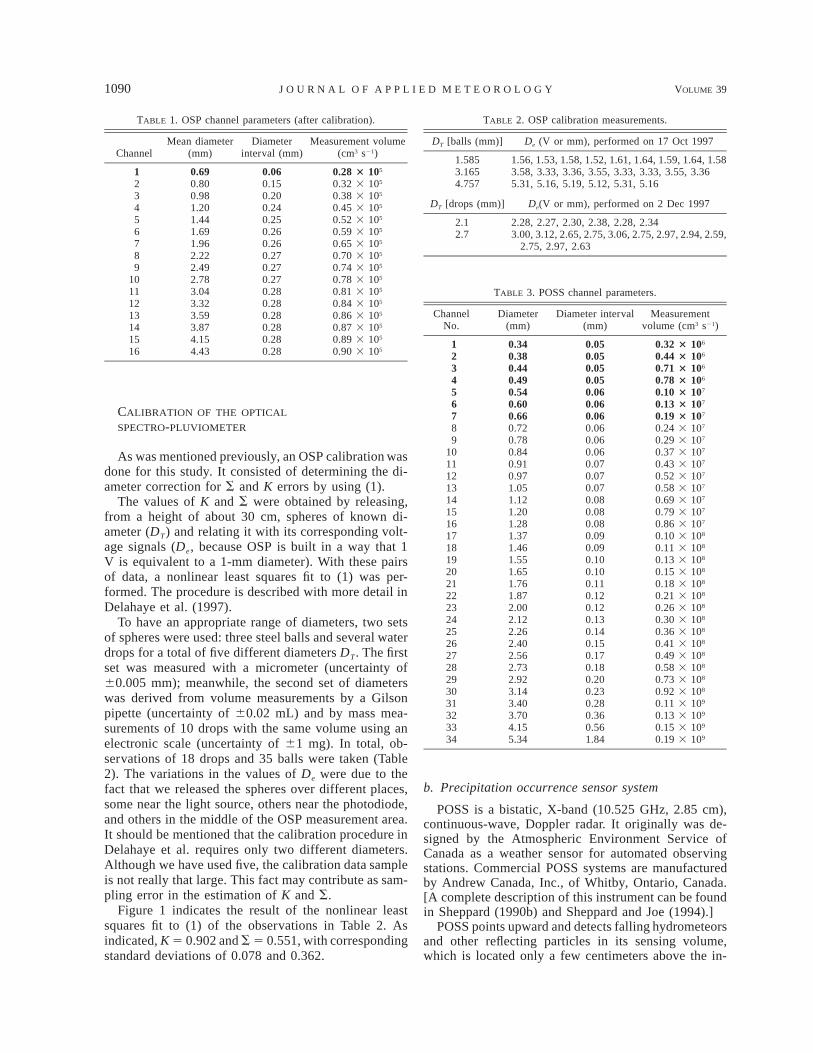
1090 VOLUME 39J O U R N A L O F A P P L I E D M E T E O R O L O G Y
TABLE 1. OSP channel parameters (after calibration).
ChannelMean diameter
(mm)Diameter
interval (mm)Measurement volume
(cm3 s21)
123456789
0.690.800.981.201.441.691.962.222.49
0.060.150.200.240.250.260.260.270.27
0.28 3 105
0.32 3 105
0.38 3 105
0.45 3 105
0.52 3 105
0.59 3 105
0.65 3 105
0.70 3 105
0.74 3 105
10111213141516
2.783.043.323.593.874.154.43
0.270.280.280.280.280.280.28
0.78 3 105
0.81 3 105
0.84 3 105
0.86 3 105
0.87 3 105
0.89 3 105
0.90 3 105
TABLE 2. OSP calibration measurements.
DT [balls (mm)] De (V or mm), performed on 17 Oct 1997
1.5853.1654.757
1.56, 1.53, 1.58, 1.52, 1.61, 1.64, 1.59, 1.64, 1.583.58, 3.33, 3.36, 3.55, 3.33, 3.33, 3.55, 3.365.31, 5.16, 5.19, 5.12, 5.31, 5.16
DT [drops (mm)] De(V or mm), performed on 2 Dec 1997
2.12.7
2.28, 2.27, 2.30, 2.38, 2.28, 2.343.00, 3.12, 2.65, 2.75, 3.06, 2.75, 2.97, 2.94, 2.59,
2.75, 2.97, 2.63
TABLE 3. POSS channel parameters.
ChannelNo.
Diameter(mm)
Diameter interval(mm)
Measurementvolume (cm3 s21)
1234567
0.340.380.440.490.540.600.66
0.050.050.050.050.060.060.06
0.32 3 106
0.44 3 106
0.71 3 106
0.78 3 106
0.10 3 107
0.13 3 107
0.19 3 107
89
101112131415
0.720.780.840.910.971.051.121.20
0.060.060.060.070.070.070.080.08
0.24 3 107
0.29 3 107
0.37 3 107
0.43 3 107
0.52 3 107
0.58 3 107
0.69 3 107
0.79 3 107
16171819202122232425
1.281.371.461.551.651.761.872.002.122.26
0.080.090.090.100.100.110.120.120.130.14
0.86 3 107
0.10 3 108
0.11 3 108
0.13 3 108
0.15 3 108
0.18 3 108
0.21 3 108
0.26 3 108
0.30 3 108
0.36 3 108
262728293031323334
2.402.562.732.923.143.403.704.155.34
0.150.170.180.200.230.280.360.561.84
0.41 3 108
0.49 3 108
0.58 3 108
0.73 3 108
0.92 3 108
0.11 3 109
0.13 3 109
0.15 3 109
0.19 3 109
CALIBRATION OF THE OPTICAL
SPECTRO-PLUVIOMETER
As was mentioned previously, an OSP calibration wasdone for this study. It consisted of determining the di-ameter correction for S and K errors by using (1).
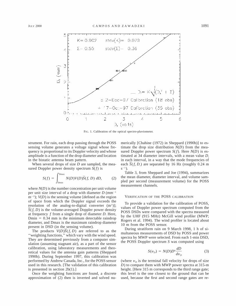
The values of K and S were obtained by releasing,from a height of about 30 cm, spheres of known di-ameter (DT) and relating it with its corresponding volt-age signals (De, because OSP is built in a way that 1V is equivalent to a 1-mm diameter). With these pairsof data, a nonlinear least squares fit to (1) was per-formed. The procedure is described with more detail inDelahaye et al. (1997).
To have an appropriate range of diameters, two setsof spheres were used: three steel balls and several waterdrops for a total of five different diameters DT. The firstset was measured with a micrometer (uncertainty of60.005 mm); meanwhile, the second set of diameterswas derived from volume measurements by a Gilsonpipette (uncertainty of 60.02 mL) and by mass mea-surements of 10 drops with the same volume using anelectronic scale (uncertainty of 61 mg). In total, ob-servations of 18 drops and 35 balls were taken (Table2). The variations in the values of De were due to thefact that we released the spheres over different places,some near the light source, others near the photodiode,and others in the middle of the OSP measurement area.It should be mentioned that the calibration procedure inDelahaye et al. requires only two different diameters.Although we have used five, the calibration data sampleis not really that large. This fact may contribute as sam-pling error in the estimation of K and S.
Figure 1 indicates the result of the nonlinear leastsquares fit to (1) of the observations in Table 2. Asindicated, K 5 0.902 and S 5 0.551, with correspondingstandard deviations of 0.078 and 0.362.
b. Precipitation occurrence sensor system
POSS is a bistatic, X-band (10.525 GHz, 2.85 cm),continuous-wave, Doppler radar. It originally was de-signed by the Atmospheric Environment Service ofCanada as a weather sensor for automated observingstations. Commercial POSS systems are manufacturedby Andrew Canada, Inc., of Whitby, Ontario, Canada.[A complete description of this instrument can be foundin Sheppard (1990b) and Sheppard and Joe (1994).]
POSS points upward and detects falling hydrometeorsand other reflecting particles in its sensing volume,which is located only a few centimeters above the in-
JULY 2000 1091C A M P O S A N D Z A W A D Z K I
FIG. 1. Calibration of the optical spectro-pluviometer.
strument. For rain, each drop passing through the POSSsensing volume generates a voltage signal whose fre-quency is proportional to its Doppler velocity and whoseamplitude is a function of the drop diameter and locationin the bistatic antenna beam pattern.
When several drops of size D are sampled, the mea-sured Doppler power density spectrum S( f ) is
Dmax
S( f ) 5 N(D)V(D)S( f, D) dD, (2)EDmin
where N(D) is the number concentration per unit volumeper unit size interval of a drop with diameter D (mm21
m23); V(D) is the sensing volume [defined as the regionof space from which the Doppler signal exceeds theresolution of the analog-to-digital converter (m3)];S( f, D) is the volume-averaged Doppler power densityat frequency f from a single drop of diameter D. Here,Dmin 5 0.34 mm is the minimum detectable raindropdiameter, and Dmax is the maximum raindrop diameterpresent in DSD (in the sensing volume).
The products V(D)S( f, D) are referred to as the‘‘weighting functions,’’ which vary with the wind speed.They are determined previously from a computer sim-ulation (assuming stagnant air), as a part of the sensorcalibration, using laboratory measurements and theo-retical values for the antenna gain patterns (Sheppard1990b). During September 1997, this calibration wasperformed by Andrew Canada, Inc., for the POSS sensorused in this research. [The validation of this calibrationis presented in section 2b(1).]
Once the weighting functions are found, a discreteapproximation of (2) then is inverted and solved nu-
merically [Chahine (1972) in Sheppard (1990b)] to es-timate the drop size distribution N(D) from the mea-sured Doppler power spectrum S( f ). Here N(D) is es-timated at 34 diameter intervals, with a mean value Di
in each interval, in a way that the mode frequencies ofeach S( f, Di) are separated by 16 Hz (roughly 0.24 ms21).
Table 3, from Sheppard and Joe (1994), summarizesthe mean diameter, diameter interval, and volume sam-pled per second (measurement volume) for the POSSmeasurement channels.
VERIFICATION OF THE POSS CALIBRATION
To provide a validation for the calibration of POSS,values of Doppler power spectrum computed from thePOSS DSDs were compared with the spectra measuredby the UHF (915 MHz) McGill wind profiler (MWP;Rogers et al. 1994). The wind profiler is located about10 m from the POSS sensor.
During stratiform rain on 9 March 1998, 1 h of si-multaneous measurements of DSD by POSS and powerspectra by MWP were selected. From each 1-min DSD,the POSS Doppler spectrum S was computed using
dD6S(y ) 5 N(D)D (3)D dy D
(where y D is the terminal fall velocity for drops of sizeD) to compare them with MWP power spectra at 315-mheight. [Here 315 m corresponds to the third range gate;this level is the one closest to the ground that can beused, because the first and second range gates are re-
1092 VOLUME 39J O U R N A L O F A P P L I E D M E T E O R O L O G Y
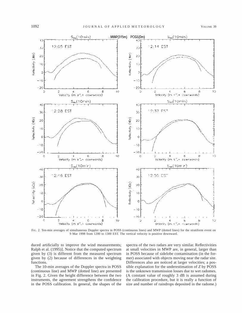
FIG. 2. Ten-min averages of simultaneous Doppler spectra in POSS (continuous lines) and MWP (dotted lines) for the stratiform event on9 Mar 1998 from 1200 to 1300 EST. The vertical velocity is positive downward.
duced artificially to improve the wind measurements;Ralph et al. (1995)]. Notice that the computed spectrumgiven by (3) is different from the measured spectrumgiven by (2) because of differences in the weightingfunctions.
The 10-min averages of the Doppler spectra in POSS(continuous line) and MWP (dotted line) are presentedin Fig. 2. Given the height difference between the twoinstruments, the agreement strengthens the confidencein the POSS calibration. In general, the shapes of the
spectra of the two radars are very similar. Reflectivitiesat small velocities in MWP are, in general, larger thanin POSS because of sidelobe contamination (in the for-mer) associated with objects moving near the radar site.Differences also are noticed at larger velocities; a pos-sible explanation for the underestimation of Z by POSSis the unknown transmission losses due to wet radomes.(A constant value of roughly 3 dB is assumed duringthe calibration procedure, but it is really a function ofsize and number of raindrops deposited in the radome.)
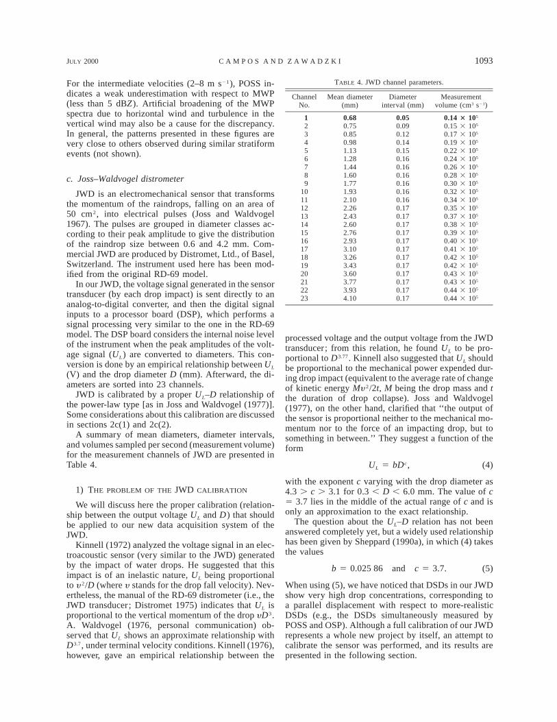
JULY 2000 1093C A M P O S A N D Z A W A D Z K I
TABLE 4. JWD channel parameters.
ChannelNo.
Mean diameter(mm)
Diameterinterval (mm)
Measurementvolume (cm3 s21)
123456789
0.680.750.850.981.131.281.441.601.77
0.050.090.120.140.150.160.160.160.16
0.14 3 105
0.15 3 105
0.17 3 105
0.19 3 105
0.22 3 105
0.24 3 105
0.26 3 105
0.28 3 105
0.30 3 105
10111213141516171819
1.932.102.262.432.602.762.933.103.263.43
0.160.160.170.170.170.170.170.170.170.17
0.32 3 105
0.34 3 105
0.35 3 105
0.37 3 105
0.38 3 105
0.39 3 105
0.40 3 105
0.41 3 105
0.42 3 105
0.42 3 105
20212223
3.603.773.934.10
0.170.170.170.17
0.43 3 105
0.43 3 105
0.44 3 105
0.44 3 105
For the intermediate velocities (2–8 m s21), POSS in-dicates a weak underestimation with respect to MWP(less than 5 dBZ). Artificial broadening of the MWPspectra due to horizontal wind and turbulence in thevertical wind may also be a cause for the discrepancy.In general, the patterns presented in these figures arevery close to others observed during similar stratiformevents (not shown).
c. Joss–Waldvogel distrometer
JWD is an electromechanical sensor that transformsthe momentum of the raindrops, falling on an area of50 cm2, into electrical pulses (Joss and Waldvogel1967). The pulses are grouped in diameter classes ac-cording to their peak amplitude to give the distributionof the raindrop size between 0.6 and 4.2 mm. Com-mercial JWD are produced by Distromet, Ltd., of Basel,Switzerland. The instrument used here has been mod-ified from the original RD-69 model.
In our JWD, the voltage signal generated in the sensortransducer (by each drop impact) is sent directly to ananalog-to-digital converter, and then the digital signalinputs to a processor board (DSP), which performs asignal processing very similar to the one in the RD-69model. The DSP board considers the internal noise levelof the instrument when the peak amplitudes of the volt-age signal (UL) are converted to diameters. This con-version is done by an empirical relationship between UL
(V) and the drop diameter D (mm). Afterward, the di-ameters are sorted into 23 channels.
JWD is calibrated by a proper UL–D relationship ofthe power-law type [as in Joss and Waldvogel (1977)].Some considerations about this calibration are discussedin sections 2c(1) and 2c(2).
A summary of mean diameters, diameter intervals,and volumes sampled per second (measurement volume)for the measurement channels of JWD are presented inTable 4.
1) THE PROBLEM OF THE JWD CALIBRATION
We will discuss here the proper calibration (relation-ship between the output voltage UL and D) that shouldbe applied to our new data acquisition system of theJWD.
Kinnell (1972) analyzed the voltage signal in an elec-troacoustic sensor (very similar to the JWD) generatedby the impact of water drops. He suggested that thisimpact is of an inelastic nature, UL being proportionalto y 2/D (where y stands for the drop fall velocity). Nev-ertheless, the manual of the RD-69 distrometer (i.e., theJWD transducer; Distromet 1975) indicates that UL isproportional to the vertical momentum of the drop yD3.A. Waldvogel (1976, personal communication) ob-served that UL shows an approximate relationship withD3.7, under terminal velocity conditions. Kinnell (1976),however, gave an empirical relationship between the
processed voltage and the output voltage from the JWDtransducer; from this relation, he found UL to be pro-portional to D3.77. Kinnell also suggested that UL shouldbe proportional to the mechanical power expended dur-ing drop impact (equivalent to the average rate of changeof kinetic energy My 2/2t, M being the drop mass and tthe duration of drop collapse). Joss and Waldvogel(1977), on the other hand, clarified that ‘‘the output ofthe sensor is proportional neither to the mechanical mo-mentum nor to the force of an impacting drop, but tosomething in between.’’ They suggest a function of theform
UL 5 bDc, (4)
with the exponent c varying with the drop diameter as4.3 . c . 3.1 for 0.3 , D , 6.0 mm. The value of c5 3.7 lies in the middle of the actual range of c and isonly an approximation to the exact relationship.
The question about the UL–D relation has not beenanswered completely yet, but a widely used relationshiphas been given by Sheppard (1990a), in which (4) takesthe values
b 5 0.025 86 and c 5 3.7. (5)
When using (5), we have noticed that DSDs in our JWDshow very high drop concentrations, corresponding toa parallel displacement with respect to more-realisticDSDs (e.g., the DSDs simultaneously measured byPOSS and OSP). Although a full calibration of our JWDrepresents a whole new project by itself, an attempt tocalibrate the sensor was performed, and its results arepresented in the following section.
1094 VOLUME 39J O U R N A L O F A P P L I E D M E T E O R O L O G Y
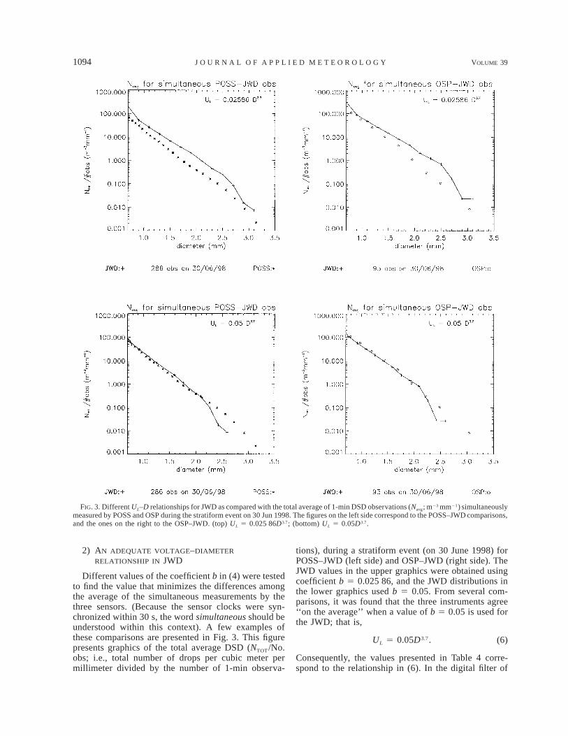
FIG. 3. Different UL–D relationships for JWD as compared with the total average of 1-min DSD observations (Navg; m23 mm21) simultaneouslymeasured by POSS and OSP during the stratiform event on 30 Jun 1998. The figures on the left side correspond to the POSS–JWD comparisons,and the ones on the right to the OSP–JWD. (top) UL 5 0.025 86D3.7; (bottom) UL 5 0.05D3.7.
2) AN ADEQUATE VOLTAGE–DIAMETER
RELATIONSHIP IN JWD
Different values of the coefficient b in (4) were testedto find the value that minimizes the differences amongthe average of the simultaneous measurements by thethree sensors. (Because the sensor clocks were syn-chronized within 30 s, the word simultaneous should beunderstood within this context). A few examples ofthese comparisons are presented in Fig. 3. This figurepresents graphics of the total average DSD (NTOT/No.obs; i.e., total number of drops per cubic meter permillimeter divided by the number of 1-min observa-
tions), during a stratiform event (on 30 June 1998) forPOSS–JWD (left side) and OSP–JWD (right side). TheJWD values in the upper graphics were obtained usingcoefficient b 5 0.025 86, and the JWD distributions inthe lower graphics used b 5 0.05. From several com-parisons, it was found that the three instruments agree‘‘on the average’’ when a value of b 5 0.05 is used forthe JWD; that is,
UL 5 0.05D3.7. (6)
Consequently, the values presented in Table 4 corre-spond to the relationship in (6). In the digital filter of

JULY 2000 1095C A M P O S A N D Z A W A D Z K I
FIG. 4. Isolines of (a) reflectivity and (b) vertical velociy (positive downward) varying with height andtime (EST), measured with the UHF (915 MHz) McGill/National Oceanic and Atmospheric Administrationwind profiler (MWP) during the period of the comparisons for the stratiform case on 14 Jun 1998.
1096 VOLUME 39J O U R N A L O F A P P L I E D M E T E O R O L O G Y
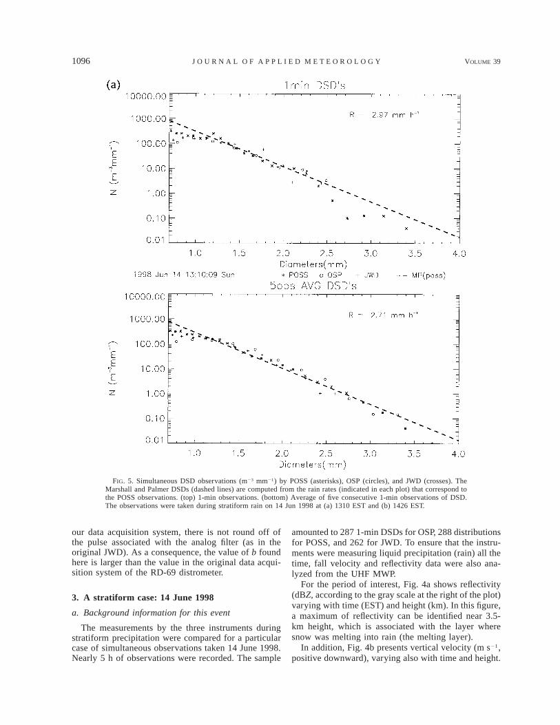
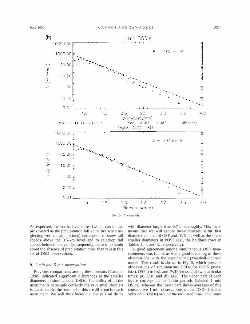
FIG. 5. Simultaneous DSD observations (m23 mm21) by POSS (asterisks), OSP (circles), and JWD (crosses). TheMarshall and Palmer DSDs (dashed lines) are computed from the rain rates (indicated in each plot) that correspond tothe POSS observations. (top) 1-min observations. (bottom) Average of five consecutive 1-min observations of DSD.The observations were taken during stratiform rain on 14 Jun 1998 at (a) 1310 EST and (b) 1426 EST.
our data acquisition system, there is not round off ofthe pulse associated with the analog filter (as in theoriginal JWD). As a consequence, the value of b foundhere is larger than the value in the original data acqui-sition system of the RD-69 distrometer.
3. A stratiform case: 14 June 1998
a. Background information for this event
The measurements by the three instruments duringstratiform precipitation were compared for a particularcase of simultaneous observations taken 14 June 1998.Nearly 5 h of observations were recorded. The sample
amounted to 287 1-min DSDs for OSP, 288 distributionsfor POSS, and 262 for JWD. To ensure that the instru-ments were measuring liquid precipitation (rain) all thetime, fall velocity and reflectivity data were also ana-lyzed from the UHF MWP.
For the period of interest, Fig. 4a shows reflectivity(dBZ, according to the gray scale at the right of the plot)varying with time (EST) and height (km). In this figure,a maximum of reflectivity can be identified near 3.5-km height, which is associated with the layer wheresnow was melting into rain (the melting layer).
In addition, Fig. 4b presents vertical velocity (m s21,positive downward), varying also with time and height.
JULY 2000 1097C A M P O S A N D Z A W A D Z K I
FIG. 5. (Continued)
As expected, the vertical velocities (which can be ap-proximated as the precipitation fall velocities when ne-glecting vertical air motions) correspond to snow fallspeeds above the 3.5-km level and to raindrop fallspeeds below this level. Consequently, there is no doubtabout the absence of precipitation other than rain in thisset of DSD observations.
b. 1-min and 5-min observations
Previous comparisons among these sensors (Campos1998) indicated significant differences at the smallerdiameters of simultaneous DSDs. The ability of all theinstruments to sample correctly the very small dropletsis questionable; the reasons for this are different for eachinstrument. We will thus focus our analysis on drops
with diameter larger than 0.7 mm, roughly. This focusmeans that we will ignore measurements in the firstdiameter channel of OSP and JWD, as well as the sevensmaller diameters in POSS (i.e., the boldface rows inTables 1, 4, and 3, respectively).
A good agreement among simultaneous DSD mea-surements was found, as was a good matching of theseobservations with the exponential (Marshall–Palmer)model. This result is shown in Fig. 5, which presentsobservations of simultaneous DSDs for POSS (aster-isks), OSP (circles), and JWD (crosses) at two particulartimes: (a) 1310 and (b) 1426. The upper part of eachfigure corresponds to 1-min periods (labeled 1 minDSDs), whereas the lower part shows averages of fiveconsecutive 1-min observations of the DSDs (labeled5obs AVG DSDs) around the indicated time. The 5-min
1098 VOLUME 39J O U R N A L O F A P P L I E D M E T E O R O L O G Y
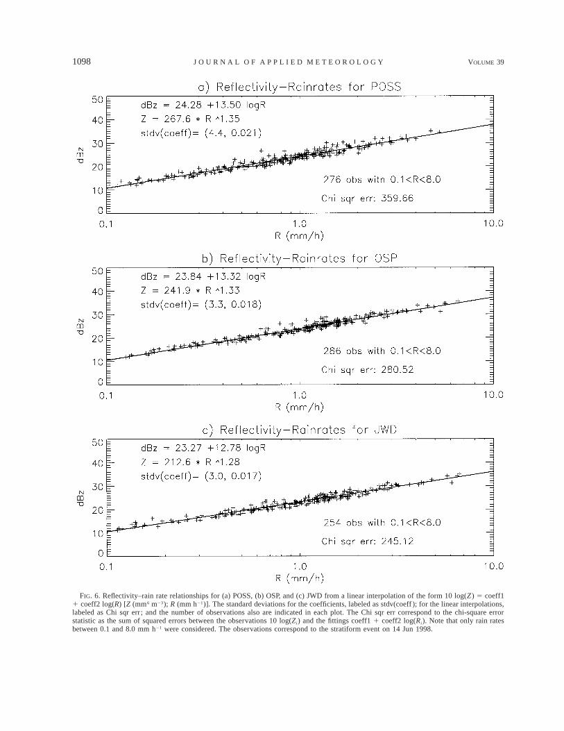
FIG. 6. Reflectivity–rain rate relationships for (a) POSS, (b) OSP, and (c) JWD from a linear interpolation of the form 10 log(Z ) 5 coeff11 coeff2 log(R) [Z (mm6 m23); R (mm h21)]. The standard deviations for the coefficients, labeled as stdv(coeff ); for the linear interpolations,labeled as Chi sqr err ; and the number of observations also are indicated in each plot. The Chi sqr err correspond to the chi-square errorstatistic as the sum of squared errors between the observations 10 log(Zi) and the fittings coeff1 1 coeff2 log(Ri). Note that only rain ratesbetween 0.1 and 8.0 mm h21 were considered. The observations correspond to the stratiform event on 14 Jun 1998.
JULY 2000 1099C A M P O S A N D Z A W A D Z K I
averages are more stable measurements. Denoted rainrates (mm h21) are computed from the respective POSSdistributions using
`p3R 5 D y N(D) dD. (7)E D6 0
These rain rates are used to obtain the theoretical Mar-shall and Palmer DSDs (dashed lines). Although somedifferences can be seen, the agreement among the in-struments is encouraging. We would like to knowwhether and to what extent these measurement differ-ences affect the estimation of rain rate–reflectivity re-lationships.
c. Reflectivity–rain rate relationships
For 0.1 # R # 8.0 mm h21, and during the samestratiform event, radar reflectivity factors (mm6 m23)were computed from
`
6Z 5 D N(D) dD. (8)E0
A Z–R relationship for each instrument then was derivedfrom a linear regression [minimizing the chi-square er-ror statistic, with no weighting (Press et al. 1989)] be-tween 10 log(Z) and log(R) [10 log(Z) as a function oflog(R)]. The results are indicated in Fig. 6, where dBZstands for 10 log(Z). The differences in the relationshipsare of the same order of magnitude as the differencesgenerally found in distinct climatic regions (Battan1973; Ulbrich 1983). Therefore, the Z–R relationshipsare highly instrument dependent.
To give an idea of the statistical significance of thedifferences in the coefficients of the Z–R relations, thevalues of the standard deviations of these coefficientsare included in Fig. 6 (and Fig. 7). Assuming a standardnormal probability distribution, the 32% level of sig-nificance (in a two-tailed test) corresponds to plus orminus one standard deviation around the value of thecorresponding coefficient. In most of the cases, the dif-ferences in the coefficients are even larger than plus orminus two standard deviations, which means that theyare different, with significance smaller than 4.5%.
The chi-square error statistic, defined as the sum ofsquared errors between 10 log(Zi) and coeff1 1 coeff2log(Ri), is a measure of the dispersion in Z from a givenZ–R relation. (The value of this statistic is indicated, foreach sensor, in Fig. 6.) We then would expect POSS tohave the smallest dispersion because of its bigger samplevolume, but it has the largest chi-square error.
The reason for POSS having larger dispersion in theZ–R relation resides in its larger measurement volume.Zawadzki (1984) notes that R is more-tightly correlatedwith Z derived from distrometer observations (smallsample volume) than with Z measured by radar (largesample volume). To explain this result, Chandrasekarand Bringi (1987) numerically simulated radar and sur-
face distrometer measurements of rainfall to explainwhy the correlation is smaller for radar-measured re-flectivity. They propose a Z–R relation constructed byboth physical and statistical relationships that exist be-tween the reflectivity and the rain rate. The statisticalcorrelation is a consequence of computing Z and R fromthe same sample. These authors suggest that the increasein variance of Z–R relations with instrument samplingvolume is explained by the decrease in statistical cor-relation with increasing sample volume. Comparing thedifferent measurement volumes of each instrument (Ta-bles 1, 2, and 4), and Fig. 6, we can see clearly howPOSS has much larger measurement volumes, standarddeviations in the coefficients of the Z–R relation, andchi-square error statistic in comparison with the othertwo sensors. Then, the observed greatest dispersion ofthe Z–R relations in POSS may be due to the effectdiscussed by Chandrasekar and Bringi.
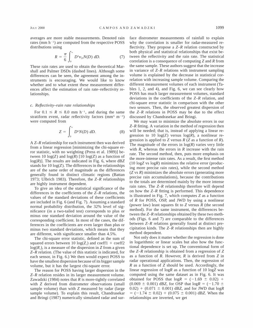
We may want to minimize the absolute errors in ourZ–R fitting. A variation in the method of regression thenwill be needed; that is, instead of applying a linear re-gression to 10 log(Z) versus log(R), a nonlinear re-gression is applied to Z versus R (Z as a function of R).The magnitude of the errors in log(R) varies very littlewith R, whereas the errors in R increase with the rainrate. The second method, then, puts more emphasis onthe more-intense rain rates. As a result, the first method(10 logZ vs logR) minimizes the relative error (produc-ing more precise rain rates), while the second method(Z vs R) minimizes the absolute errors (generating moreprecise rain accumulations), because the contributionsto the totals are determined mainly by the more intenserain rates. The Z–R relationship therefore will dependon how the Z–R fitting is performed. This dependenceis illustrated in Fig. 7, which computes Z as a functionof R for POSS, OSP, and JWD by using a nonlinear(power law) least squares fit to Z versus R (the secondmethod). For the same instrument, the differences be-tween the Z–R relationships obtained by these two meth-ods (Figs. 6 and 7) are comparable to the differencesbetween Z–R relations generally found at distinct pre-cipitation kinds. The Z–R relationships then are highlymethod dependent.
Not only does it matter whether the regression is donein logarithmic or linear scales but also how the func-tional dependence is set up. The conventional form ofthe Z–R relationship is obtained from a regression of Zas a function of R. However, R is derived from Z inradar operational applications. Then, the regression ofR as a function of Z should be used. Accordingly, thelinear regression of logR as a function of 10 logZ wascomputed using the same dataset as in Fig. 6. It wasobtained for POSS that logR 5 (21.69 6 0.02) 1(0.069 6 0.001) dBZ, for OSP that logR 5 (21.70 60.02) 1 (0.071 6 0.001) dBZ, and for JWD that logR5 (21.74 6 0.02) 1 (0.075 6 0.001) dBZ. When therelationships are inverted, we get
1100 VOLUME 39J O U R N A L O F A P P L I E D M E T E O R O L O G Y
FIG. 7. Reflectivity–rain rate relationships for (a) POSS, (b) OSP, and (c) JWD from a nonlinear interpolation of the form Z 5 coeff1Rcoeff2
between Z (mm6 m23) and R (mm h21). Only rain rates between 0.1 and 8.0 were considered. The standard deviations for the coefficients,labeled as stdv(coeff ); for the nonlinear interpolations, labeled as stdv(dBz); and the number of observations used also are indicated. Theobservations correspond to the stratiform event on 14 Jun 1998.

JULY 2000 1101C A M P O S A N D Z A W A D Z K I
1.4560.02 1.4160.02Z 5 (281 6 4)R , Z 5 (248 6 3)R ,1.3360.02Z 5 (209 6 2)R
for the three instruments, respectively. These relation-ships are significantly different from those given in Fig.6. In fact, the differences will increase with increasingscatter of the Z–R plots. In a data sample coming froma less-homogeneous precipitation than the one presentedhere, the difference in the Z–R relationship can be verylarge, depending on which of the two parameters is tak-en as the independent variable.
4. Discussion
After calibration of JWD, OSP, and POSS, 1-min ob-servations of DSD have been taken at Montreal duringone summer season. It was noticed that, if data fromeach instrument are analyzed separately and stratifiedby rain rate (as determined by the particular instrument),a Marshal–Palmer-type relationship is found for thethree sets. Previous comparisons between simultaneousmeasurements of DSD by POSS, OSP, and JWD (Cam-pos 1998) indicated significant differences, particularlyat the smaller diameters. Accordingly, drop concentra-tions at diameters near 0.7 mm or less are eliminatedfrom a sample of the continental, stratiform rain (Fig.4). The agreement among the sensors is very good forthe DSDs during the event (Fig. 5). During the samestratiform case, Z–R relationships were computed foreach instrument by applying a linear regression between10 logZ and logR. The Z–R relations obtained are (Fig.6):
1.35Z 5 267.6R , for POSS;1.33Z 5 241.9R , for OSP; and1.28Z 5 212.6R , for JWD.
The differences among these three relations are verymuch comparable to the variation in relationships fromdistinct climatic regions. For example, Z 5 256R1.41 wasobtained from rain at Island Beach, New Jersey [Muellerand Sims (1966) in Battan (1973)]; Z 5 240R1.30 wasderived for rain in Lwire, Congo [Diem (1966) in Battan(1973)]; and Z 5 215R1.34 was found during stratiformrain at Lexington, Massachusetts [Atlas and Chmela(1957) in Battan (1973)].
When changing the analysis method for obtaining theZ–R relations (i.e., applying a nonlinear regression be-tween Z and R), a significant variation was also found(Fig. 7): Z 5 208.5R1.69 for POSS; Z 5 195.0R1.61 forOSP; and Z 5 119.8R1.81 for JWD. These three relationsalso agree with others mentioned in the literature—suchas Z 5 204R1.70, which corresponds to showers in Kiev,ex-USSR [Muchnik (1961) in Battan (1973)]; Z 5200R1.6, the Marshall and Palmer relation for continen-tal, stratiform rain; and Z 5 109R1.64, derived from oro-graphic, monsoon rains in Kandia, India (Ramana Mur-thy and Gupta (1959) in Battan (1973).
Therefore, we have found not just a strong depen-dence of the Z–R relationships with the sensor but alsowith its data analysis method. Extreme caution is inorder when Z–R relationships from different sources arecompared. It therefore is recommended that any Z–Rrelationship to be published should include informationof the sample size, the regression setup, and the statis-tical estimation algorithm used.
Acknowledgments. Much of this work was based onthe first author’s M.S. thesis (Campos 1998); Camposwas partially supported by a fellowship from the WorldMeteorological Organization and the Instituto Meteo-rologico Nacional of Costa Rica. The authors are in-debted to the Atmospheric Environment Service (AES)of Canada and the Centre de Recherches en Physiquede l’Environnement Terrestre et Planetaire (CETP) forproviding for this experiment POSS and OSP, respec-tively. Important contributions concerning the descrip-tion of the instruments used in this research were givenby Frederic Fabry, from the McGill Radar Observatory;Peter Gole, from the Electromagnetism and Methods ofAnalysis division at CETP; and Brian Sheppard andKenneth Wu, from AES at Downsview, Ontario, Can-ada. Wayne Zelmer, from Litton Systems Canada at Hal-ifax, Nova Scotia, Canada, developed the new data ac-quisition system of our JWD. The collaboration givenby Dr. William Brown, from the Atmospheric Technol-ogy Division at the National Center for AtmosphericResearch, when calibrating the OSP also was very ap-preciated.
REFERENCES
Atlas, D., and A. C. Chmela, 1957: Physical-synoptic variations ofdrop-size parameters. Proc. Sixth Weather Radar Conf., Boston,MA, Amer. Meteor. Soc., 21–30.
Battan, L. J., 1973: Radar Observation of the Atmosphere. Universityof Chicago Press, 324 pp.
Campos, E., 1998: Measurements of raindrop size distributions bythree different sensors. M.S. thesis, Dept. of Atmospheric andOceanic Sciences, McGill University, 96 pp. [Available fromRedpath Library, McGill University, Montreal, PQ H3A 2K6,Canada.]
Chahine, M., 1972: A general relaxation method for inverse solutionof the full radiative transfer equation. J. Atmos. Sci., 29, 741–747.
Chandrasekar, V., and V. N. Bringi, 1987: Simulation of radar re-flectivity and surface measurements of rainfall. J. Atmos. Oce-anic Technol., 4, 464–478.
Delahaye, J. Y., J. P. Vinson, C. Gloaguen, and P. Gole, 1997: LeSpectropluviometre CETP. Document de Travail CETP, Version3.1, 31 pp. [Available online at http://www.cetp.ipsl.fr/lactiv/21mineu/ema/Spectrol.html.]
Diem, M., 1966: Rains in the Arctic, temperate, and tropical zones.Science Report, Meteorologisches Institut Technische Hochs-chule, Karlsruhe, Germany, 93 pp.
Distromet, 1975: Distrometer RD-69: Instruction manual. Distromet,Ltd., 18 pp. [Available from Distromet, Ltd., P.O. Box 33, CH-4020 Basel, Switzerland.]
Gunn, R., and G. D. Kinzer, 1949: The terminal velocity of fall forwater drops in stagnant air. J. Meteor., 6, 243–248.
Hauser, D., P. Amayenc, B. Nutten, and P. Waldteufel, 1984: A new
1102 VOLUME 39J O U R N A L O F A P P L I E D M E T E O R O L O G Y
optical instrument for simultaneous measurements of raindropdiameter and fall speed distribution. J. Atmos. Oceanic Technol.,1, 256–269.
Joss, J., and A. Waldvogel, 1967: Ein spektrograph fur Nieder-shlagstropfen mit automatischer Auswertung (A spectrograph forthe automatic analysis of raindrops). Pure Appl. Geophys., 68,240–246., and , 1977: Comments on ‘‘Some observations on the Joss–Waldvogel rainfall disdrometer.’’ J. Appl. Meteor., 16, 112–114.
Kinnell, P. I. A., 1972: The acoustic measurement of water dropimpacts. J. Appl. Meteor., 11, 691–694., 1976: Some observations on the Joss–Waldvogel rainfall dis-drometer. J. Appl. Meteor., 15, 499–502.
Marshall, J. S., and W. McK. Palmer, 1948: The distribution of rain-drops with size. J. Meteor., 5, 165–166.
Muchnik, V. M., 1961: O tochnosti izmereniya intensivnosti dozhdeiradiolokatsionnymi metodami (The accuracy of radar rain-in-tensity measurements). Meteor. Gidrol., 2, 44–47.
Mueller, E. A., and A. L. Sims, 1966: The influence of samplingvolume on raindrop size spectra. Proc. 12th Conf. on RadarMeteorology, Norman, OK, Amer. Meteor. Soc., 135–141.
Press, W., B. Flannery, S. Teukolsky, and W. Vetterling, 1989: Nu-merical Recipes in Pascal: The Art of Scientific Computing.Cambridge University Press, 759 pp.
Ralph, F. M., P. J. Neiman, D. W. van de Kamp, and D. C. Law, 1995:Using spectral moment data from NOAA’s 404-MHz radar windprofilers to observe precipitation. Bull. Amer. Meteor. Soc., 76,1717–1739.
Ramana Murty, Bh. V., and S. C. Gupta, 1959: Precipitation char-acteristics based on raindrop size measurements at Delhi andKhandala during southwest monsoon. J. Sci. Ind. Res., 18A, 352–371.
Rogers, R. R., S. A. Cohn, W. L. Ecklund, J. S. Wilson, and D. A.Carter, 1994: Experience from one year of operating a boundary-layer profiler in the center of a large city. Ann. Geophys., 12,529–540.
Sauvageot, H., and J.-P. Lacaux, 1995: The shape of averaged dropsize distributions. J. Atmos. Sci., 52, 1070–1083.
Sheppard, B. E., 1990a: Effect of irregularities in the diameter clas-sification of raindrops by the Joss–Waldvogel disdrometer. J.Atmos. Oceanic Technol., 7, 180–183., 1990b: Measurement of raindrop size distributions using a smallDoppler radar. J. Atmos. Oceanic Technol., 7, 255–268., and P. I. Joe, 1994: Comparison of raindrop size distributionmeasurements by a Joss–Waldvogel disdrometer, a PMS 2DGspectrometer, and a POSS Doppler radar. J. Atmos. OceanicTechnol., 11, 874–887.
Ulbrich, C. W., 1983: Natural variations in the analytical form of theraindrop size distribution. J. Climate Appl. Meteor., 22, 1764–1775.
Zawadzki, I., 1984: Factors affecting the precision of radar mea-surements of rain. Preprints, 22d Conf. on Radar Meteorology,Zurich, Switzerland, Amer. Meteor. Soc., 251–256., and M. de Agostinho Antonio, 1988: Equilibrium raindrop sizedistributions in tropical rain. J. Atmos. Sci., 45, 3452–3459.