Costs, safety and uncertainties of CO2 infrastructure ...
359
Costs, safety and uncertainties of CO 2 infrastructure development
-
Upload
khangminh22 -
Category
Documents
-
view
2 -
download
0
Transcript of Costs, safety and uncertainties of CO2 infrastructure ...

Costs, safety and uncertainties of CO2 infrastructure development

This research was conducted under the auspices of the Graduate School for Socio‐Economic and Natural Sciences of the Environment (SENSE).
The research presented in this dissertation has been carried out at Utrecht University in the context of the CATO‐2 program. CATO‐2 is the Dutch national research program on CO2 capture and storage (CCS). The program is financially supported by the Dutch government (Ministery of Economic Affairs) and the CATO‐2 consortium partners. Cover design: Aukje’s Studio Printed by: proefschriftmaken.nl Published by: Uitgeverij BOXPress, ‘s‐Hertogenbosch ISBN: 978‐90‐393‐6387‐4

Costs, safety and uncertainties of CO2 infrastructure development
Kosten, veiligheid en onzekerheden van CO2 infrastructuur ontwikkeling (met een samenvatting in het Nederlands)
Proefschrift
ter verkrijging van de graad van doctor aan de Universiteit Utrecht
op gezag van de rector magnificus, prof. dr. G.J. van der Zwaan,
ingevolge het besluit van het college voor promoties
in het openbaar te verdedigen op
vrijdag 4 september 2015 des ochtends te 10.30 uur
door
Marlinde Marissa Jasmijn Knoope
geboren op 7 november 1986 te Helvoirt

Promotor: Prof.dr. A.P.C. Faaij
Copromoter: Dr. C.A. Ramírez

v
Table of Contents Chapter 1: Introduction ................................................................................................. 1
Climate change and the role of carbon dioxide capture and storage .................. 1 1.1 Carbon dioxide capture and storage .................................................................... 3 1.2 The role of CO2 transport and main knowledge gaps .......................................... 4 1.3
Costs of CO2 transport ..................................................................................... 6 1.3.1 Configurations for CO2 transport ..................................................................... 7 1.3.2 Risk and safety considerations ........................................................................ 9 1.3.3
Objectives and research questions .................................................................... 10 1.4 Outline of the thesis ........................................................................................... 11 1.5 References ......................................................................................................... 12 1.6
Chapter 2: A state‐of‐the‐art review of techno‐economic models predicting the costs of CO2 pipeline transport ................................................................................................. 19
Introduction ....................................................................................................... 21 2.1 Methodology ...................................................................................................... 23 2.2 CO2 properties for pipeline transport ................................................................ 26 2.3 Review of cost models in literature ................................................................... 27 2.4
Models for capital costs of CO2 pipelines ‐ state‐of‐the‐art review .............. 29 2.4.1 Models for O&M costs of pipelines ............................................................... 39 2.4.2 Models for capital costs of pumping stations ................................................ 39 2.4.3 Models for energy consumption, energy costs and fixed O&M costs of 2.4.4
pumping stations ........................................................................................................ 40 Evaluating the economic pipeline and pumping station cost models ................ 42 2.5
Evaluation of pipeline cost models ................................................................ 42 2.5.1 Regional differences ...................................................................................... 46 2.5.2 Analysis of results for pipeline capital costs .................................................. 48 2.5.3 Analysis of results for pipeline O&M costs .................................................... 49 2.5.4 Analysis of results for the capital cost models of pumping station ............... 51 2.5.5 Analysis of results for O&M costs, energy consumption and levelized costs 2.5.6
for pumping stations ................................................................................................... 52 Review of pipeline diameter models applied in literature ................................. 53 2.6
Comparison of diameter models ................................................................... 55 2.6.1 Sensitivity analysis ......................................................................................... 61 2.6.2
Identification of characteristics for cost models best suited for specific 2.7applications ......................................................................................................................... 62
General costs comparison of CCS with other technologies ........................... 63 2.7.1 System analysis over time ............................................................................. 65 2.7.2
Conclusions ........................................................................................................ 65 2.8 Knowledge gaps ................................................................................................. 67 2.9 References ......................................................................................................... 69 2.10

Table‐of‐contents
vi
Chapter 3: Improved cost models for optimizing CO2 pipeline configuration for point‐to‐ point pipelines and simple networks ............................................................................ 77
Introduction ....................................................................................................... 78 3.1 CO2 properties for pipeline transport ................................................................ 80 3.2 Description of the cost minimization process .................................................... 81 3.3
Cost minimization of one pipeline in a single type of terrain ........................ 83 3.3.1 Cost minimization of a pipeline crossing different types of terrain .............. 86 3.3.2 Feeders to and distribution pipelines from the trunkline ............................. 89 3.3.3 Timing ............................................................................................................ 90 3.3.4
Development of cost models for CO2 transport ................................................. 91 3.4 Pipeline .......................................................................................................... 91 3.4.1 Compressor .................................................................................................... 94 3.4.2 Pumping stations ........................................................................................... 96 3.4.3
Results ................................................................................................................ 97 3.5 Pipeline cost model ....................................................................................... 97 3.5.1 Cost minimization of point‐to‐point pipelines ............................................... 99 3.5.2 Pipeline crossing different types of terrain ................................................. 102 3.5.3 Simple network approach ............................................................................ 103 3.5.4 Timing aspects ............................................................................................. 108 3.5.5 Implications of the system boundaries ........................................................ 109 3.5.6 Sensitivity analysis ....................................................................................... 111 3.5.7
Conclusion ........................................................................................................ 114 3.6 References ....................................................................................................... 116 3.7
Chapter 4: The influence of risk mitigation measures on the risks, costs and routing of CO2 pipelines ............................................................................................................. 121
Introduction ..................................................................................................... 122 4.1 Methodology and data ..................................................................................... 124 4.2
Optimal configuration of specific case studies ............................................ 124 4.2.1 Dispersion and consequences of a CO2 release ........................................... 128 4.2.2 Locational and societal risk .......................................................................... 130 4.2.3 Failure frequency of base scenario .............................................................. 132 4.2.4 The influence of risk mitigation measures on costs and failure frequency . 135 4.2.5 Analyzing the consequences of risks on the routing and costs of pipelines 140 4.2.6
Results .............................................................................................................. 144 4.3 Optimization process ................................................................................... 144 4.3.1 Pipeline costs and failure frequency with additional mitigation measures . 144 4.3.2 Lethality distances ....................................................................................... 146 4.3.3 Locational risk .............................................................................................. 147 4.3.4 Implementation of risk mitigation measures or rerouting .......................... 148 4.3.5 Implication of societal risk contours ............................................................ 153 4.3.6 Vertical versus horizontal release ................................................................ 153 4.3.7
Discussion ......................................................................................................... 156 4.4 Conclusions ...................................................................................................... 157 4.5

Table‐of‐contents
vii
References ....................................................................................................... 158 4.6 Chapter 5: Investing in CO2 transport infrastructure under uncertainty: A comparison between ships and pipelines ...................................................................................... 165
Introduction ..................................................................................................... 166 5.1 Real option theory ........................................................................................... 168 5.2 CO2 transportation chains ................................................................................ 168 5.3 Method ............................................................................................................ 171 5.4
Net present value approach ........................................................................ 171 5.4.1 Real option approach ................................................................................... 172 5.4.2
Input data for the case study ........................................................................... 176 5.5 Case study .................................................................................................... 179 5.5.1 Pipeline design and costs ............................................................................. 181 5.5.2 Ship design and costs ................................................................................... 184 5.5.3
Results .............................................................................................................. 187 5.6 Pipeline versus ships with the NPV approach .............................................. 187 5.6.1 Pipeline versus ships with real option approach ......................................... 190 5.6.2
Discussion ......................................................................................................... 197 5.7 Comparison with the literature ................................................................... 197 5.7.1 Limitations of this study .............................................................................. 198 5.7.2
Conclusions and further research recommendations ...................................... 198 5.8 Conclusions .................................................................................................. 198 5.8.1 Further research recommendations ............................................................ 200 5.8.2
References ....................................................................................................... 201 5.9 Chapter 6: The influence of uncertainty in the development of a CO2 infrastructure network. ................................................................................................................... 209
Introduction ..................................................................................................... 210 6.1 Method ............................................................................................................ 212 6.2
Real option approach ................................................................................... 212 6.2.1 Perfect foresight .......................................................................................... 218 6.2.2
Case study ........................................................................................................ 219 6.3 Input variables and uncertainties ................................................................ 219 6.3.1 Capture locations and costs ......................................................................... 222 6.3.2 Storage location and costs ........................................................................... 224 6.3.3 Pipeline distances and transportation costs ................................................ 225 6.3.4 Scenarios ...................................................................................................... 226 6.3.5
Results .............................................................................................................. 227 6.4 Real option approach ....................................................................................... 228 6.5
Perfect foresight and comparison with the ROA ......................................... 234 6.5.1 Discussion and conclusion ................................................................................ 235 6.6
Considerations regarding the ROA and PF model ....................................... 236 6.6.1 Summary and discussion of main results ..................................................... 236 6.6.2 Policy implications and recommendations .................................................. 238 6.6.3
Table‐of‐contents
viii
Research recommendations ........................................................................ 238 6.6.4 References ....................................................................................................... 239 6.7
Chapter 7: Summary, conclusions and recommendations ........................................... 245
Background ...................................................................................................... 245 7.1 Objective and research questions .................................................................... 246 7.2 Summary of the findings per chapter .............................................................. 246 7.3 Answering the research questions ................................................................... 250 7.4 Final remarks .................................................................................................... 255 7.5 Key research and policy recommendations ..................................................... 256 7.6 References ....................................................................................................... 257 7.7
Chapter 8: Samenvatting, conclusies en aanbevelingen .............................................. 261
Achtergrond ..................................................................................................... 261 8.1 Doelstelling en onderzoeksvragen ................................................................... 262 8.2 Samenvatting van de resultaten per hoofdstuk ............................................... 262 8.3 Beantwoording van de onderzoeksvragen ...................................................... 267 8.4 Slotopmerkingen .............................................................................................. 273 8.5 Belangrijkste onderzoeks‐ en beleidsaanbevelingen ....................................... 274 8.6
Chapter 9: Annexes ................................................................................................... 277
Chapter 2 .......................................................................................................... 277 9.1 Annex A: Constants and detailed cost data ................................................. 277 9.1.1
Chapter 3 .......................................................................................................... 284 9.2 Annex B: Additional equations .................................................................... 284 9.2.1 Annex C: Verification of diameter and thickness model.............................. 285 9.2.2 Annex D: Compression costs of FEED studies and vendor quotations ........ 291 9.2.3 Annex E: Effect of a different MAOP. .......................................................... 291 9.2.4 Annex F: Additional results point‐to‐point pipelines ................................... 292 9.2.5 Annex G: Additional results sensitivity analysis ........................................... 294 9.2.6
Chapter 4 .......................................................................................................... 309 9.3 Annex H: EFFECTS and RISKCURVES ............................................................ 309 9.3.1 Annex I: Additional literature review and results ........................................ 314 9.3.2
Chapter 6 .......................................................................................................... 320 9.4 Annex J: Objective function and constraints for perfect foresight model ... 320 9.4.1 Annex K: Compression costs ........................................................................ 323 9.4.2 Annex L: Intermediate results from the real option approach .................... 324 9.4.3 Annex M: Detailed results from the perfect foresight model ..................... 339 9.4.4
References ....................................................................................................... 340 9.5 Dankwoord ............................................................................................................... 345 Curriculum Vitae ........................................................................................................ 347 Sense certificate ....................................................................................................... 348

ix
Abbreviations and units
ABEX Abandonment expenditures Bio‐CCS Bio‐energy combined with CCSCAPEX Capital expenditures CCGT Combined cycle gas turbineCCS Carbon dioxide capture and storage CHP Combined heat and powerCO2 Carbon dioxideCRF Capital recovery factorDECC British Department of Energy and Climate Change EGIG European gas pipeline incident data groupEIA Energy Information AdministrationEOR Enhanced oil recoveryEU European UnionFEED Front end engineering designFERC U.S. Federal Energy Regulatory CommissionGBM Geometric Brownian motionGCCSI Global CCS instituteGEA Global energy assessmentGJ Giga‐JouleGt Giga‐tonneGWh Gigawatt‐hourID Inner diameterIEA International Energy AgencyIEA GHG International Energy Agency Greenhouse Gas Research and Development
Programme IPCC International Panel of Climate Changekg kilogramskJ kilo Jouleskm kilometerkt kilotonnekW kilowattkWh kilowatt‐hourLC Levelized costsLHV Lower heating valueLSMC Least squares Monte Carlo approach M€ Million EuroMAOP Maximum allowable operation pressureMILP Mixed integer linear programmingmm millimeterMPa Mega PascalMt MegatonneMW Megawatt

Abbreviations and units
x
MWh Megawatt‐hourNGCC Natural gas combined cycleNIMBY Not in my backyardNPS Nominal pipe sizeNpumps Number of pumping stationsNPV Net present valueO&M Operation and maintence OD Outer diameterOECD Organisation for Economic Co‐operation and DevelopmentOPEX Operational expenditures PC Pulverized coal power plant PF Perfect foresightPHMSA Pipeline and hazardous materials and safety administrationPinlet Pressure inlet of the pipeline Poutlet Presure outlet of the pipeline ppmv Parts per million volumeptp Point‐to‐point QRA Quantitative risk assessmentRIVM Dutch National Institute for Public Health and the Environment ROA Real option approachROW Right‐of‐wayRRR Reasonable rate of returnTrunk TrunklineU.S. or USA United States of AmericaUCCI Upstream capital cost indexUK United KingdomUKOPA United Kingdom Onshore Pipeline Operator’s AssociationUNFCC United Nation Framework Convention on Climate ChangeZEP European Technology Platform for Zero Emission Fossil Fuel Power Plants ΔP Pressure drop

1
Chapter 1: Introduction
Climate change and the role of carbon dioxide capture and 1.1storage
One of the major challenges for the coming century is to limit drastic climate change. According to the International Panel of Climate Change, warming of the climate system is unequivocal (IPCC, 2013). First signals of climate change are already visible, the amounts of snow and ice in the Northern Hemisphere have diminished, atmosphere and oceans have warmed up, and sea level has risen since 1950 (IPCC, 2013). Especially, the speed of the observed changes is unprecedented, if we look to previous decades and millennia (IPCC, 2013).
To avoid dangerous climate change, the parties of the United Nation Framework Convention on Climate Change (UNFCC) agreed that long‐term global temperature should not rise beyond 2°C above pre‐industrial levels (UNFCCC, 2011). It is estimated that to reach this 2°C target, CO2 emissions in the atmosphere have to stabilize at a level of 450 parts per million volume (ppmv) (IEA, 2013; Johansson et al., 2012). Nowadays, the CO2 concentration in the atmosphere is about 400 ppmv, which corresponds to an increase of 40% compared to pre‐industrial levels (IPCC, 2013). It is estimated that to reach the 450 ppmv target, a maximum of 1,000 Gt of CO2 could be emitted from 2014 onwards (IEA, 2014b). This implies that global CO2 emissions should peak around 2020, at a level only marginally higher than today (IEA, 2014b; Riahi et al., 2012). From then onwards, CO2 emissions should be reduced significantly.
Different options are available to limit CO2 emissions, like renewable energy sources (wind, solar, hydro, etc.), energy efficiency measures, switching to lower carbon intensive fuels (gas or nuclear energy) and applying carbon dioxide capture and storage (CCS). With CCS, CO2 is prevented to be emitted into the atmosphere. Consequently, a higher percentage of the world’s indicated fossil fuel reserves could be exploited without exceeding the estimated 1,000 Gt CO2 that can be emitted from 2014 onwards to reach the 450 ppmv target. It is estimated that the current world’s indicated fossil fuel reserves are equivalent to about 2,860 Gt CO2, which means that a large part of the fossil fuel reserves cannot be used, the so‐called ‘stranded assets’ (Leaton et al., 2013). CCS can reduce the amount of ‘stranded assets’ with about 125 GtCO2 up to 2050, which is a 13% increase of the carbon budget (Leaton et al., 2013).
Most studies agree that a portfolio of CO2 mitigation options are simultaneously needed to reach the required reduction of CO2 emissions (Bruckner et al., 2014; Edenhofer et al., 2010; European Commission, 2011; IEA, 2013; IEA, 2014a; Riahi et al., 2012). Figure 1.1 shows a possible pathway to reach the 450 ppmv target as reported in a recent study of the International Energy Agency (IEA). In this portfolio, 14% of the cumulative reduction is realized by CCS in 2050 (IEA, 2014a). Also other studies indicate an important role for CCS. For instance, in the Global Energy Assessment (GEA) report, it is estimated that when CCS is deployed, 9%‐38% of the primary energy mix could be coupled with CCS in 2050 (Riahi

Chapter 1
2
et al., 2012). Similar percentages of 9%‐53%, with an average of 31%, are projected in a comparison of 18 different integrated assessment models (Koelbl et al., 2014).
If CCS technology is not available, the estimated costs of realizing strong reductions in CO2 emissions will increase. Compared to any other single mitigation technology, the lack of availability of CCS is most frequently associated with the most significant cost increase (Clarke et al., 2014; Edenhofer et al., 2010; Krey et al., 2014; Riahi et al., 2012; Tavoni et al., 2012). For instance, it is indicated in the GEA report that the cumulative energy investment over the period 2010‐2050 will increase with about 11‐22% if CCS technology is not available (Riahi et al., 2012).
Furthermore, the 450 ppmv target becomes more difficult to reach if CCS technology is not available, especially if mitigation actions are postponed. For instance, some studies indicate that low greenhouse concentrations might not be attainable anymore without the presence of large‐scale deployment of CCS, if actions are postponed until 2030 (Clarke et al., 2014; Edenhofer et al., 2010; Riahi et al., 2015). Especially, bio‐energy combined with CCS (bio‐CCS) plays a key role in many low‐stabilization scenarios (Bruckner et al., 2014). An advantage of bio‐CCS is that it can result in so‐called ‘net negative’ emissions. Consequently, in the long term, bio‐CCS may compensate residual emissions in other sectors where CO2 reductions are more costly (Clarke et al., 2014).
The largest CO2 reductions are projected to be realized in the power, industrial, and transportation sectors, see Figure 1.1. The power sector is projected to decarbonize almost completely by 2050. This is realized by increased efficiency, large shares of renewables, nuclear energy and CCS (IEA, 2014a; Riahi et al., 2012). If CCS is not available, the power sector can also achieve the required CO2 reduction, but this would result in 40% higher investment costs (IEA, 2012; IEA, 2014a).
In the industrial sector, CO2 emissions are projected to be reduced by using renewable energy sources, implementing best available technologies, and adding CCS for both energy and process‐based CO2 emissions (IEA, 2014a; Riahi et al., 2012). CCS is especially an interesting option for the iron & steel, cement, and (petro)chemical sectors where is projected to capture about 40%, 34% and 28% of the sector’s direct CO2 emissions in 2050, respectively (IEA, 2014a). In total, global CO2 emissions in the industrial sector are projected to reduce with 40% in 2050, but if CCS is not available a reduction of only 15% is projected (IEA, 2012; IEA, 2014a). Hence, CCS is a key technology in the industrial sector for achieving deep cuts in its CO2 emissions.
Reductions in the transportation sector are mainly realized by energy efficiency measures, alternative low carbon fuels, and reduced mobilization demand by compact urban designs (Johansson et al., 2012). Biofuels are projected to increase their share to 20% of the total transportation fuel mix. About one third of the biofuel production is projected to be equipped with CCS in 2050, resulting in negative CO2 emissions of about 1 Gt per year (IEA, 2014a).
From Figure 1.1, it can be deduced that considerable amounts of CO2 need to be stored between 2020‐2050 and the amounts are increasing over time. Riahi et al., (2012) indicate

Introduction
3
that 55‐250 Gt is projected to be stored up to 2050. At the end of 2013, about 55 Mt CO2 was stored in total by four large scale demonstration projects and eight enhanced oil recovery projects using anthropogenic CO2 (IEA, 2014a; IEA, 2014b). The IEA indicates that to reach a 14% contribution, about 100, 1,500 and 3,400 CCS projects should be in operation in 2020, 2035 and 2050, respectively (IEA, 2009).
Figure 1.1: Projected contribution to annual emission reduction between the baseline scenario (heading to a 6 °C increase in global average temperature) and the 2°C scenario (A) of several mitigation options and (B) by sector (IEA, 2014a).
Carbon dioxide capture and storage 1.2
CCS is a generic term for different processes that capture CO2 from power or industrial plants and subsequently prevent its release into the atmosphere. Several capture technologies exist, which are often grouped in three main categories:
‐ In post‐combustion technologies, the CO2 is extracted from flue gasses. Typically, flue gasses have a low CO2 concentration (about 4‐15%) and are just above atmospheric pressure, resulting in a low CO2 partial pressure. Due to this low partial pressure, chemical absorption solvents are favored to capture the CO2. For regeneration of these kinds of solvents, a temperature swing is required. This implies that large amounts of steam are needed, which is very energy‐intensive. A main advantage of post‐combustion capture technology is that it can be retrofitted in current industrial and power plants without affecting the plant’s reliability (IPCC, 2005; Leung et al., 2014; Meerman et al., 2008).
‐ In pre‐combustion technologies, CO2 is captured before the fuel is combusted. In practice, this means that the fuel is first combusted with a stream of relatively pure O2
0
10
20
30
40
50
60
2010 2020 2030 2040 2050
Gt CO2
A
Carbon capture and storagePower generation efficiency and fuel switchingNuclearEnd‐use fuel and electricity efficiencyEnd‐use fuel switchingRenewables
0
10
20
30
40
50
60
2010 2020 2030 2040 2050
Gt CO2
B
IndustryCommercialOther transformationPowerResidentialTransport

Chapter 1
4
to a synthetic gas mainly consisting of H2 and CO. In a water‐gas shift reactor, the CO reacts with H2O to form CO2 and H2. Subsequently, the CO2 can be captured and the H2 can be used as a fuel or feedstock. Due to the higher partial pressure of the CO2, physical solvents can be used to capture the CO2. Physical solvents can be regenerated with a pressure swing, which is a less energy‐intensive process than a temperature swing (Meerman et al., 2011).
‐ In oxy‐fuel combustion, the fuel is combusted with (almost) pure O2. In this way, the flue gas is not diluted with nitrogen. After combustion, the flue gas consists mainly of water vapor and CO2. After condensation of the water vapor, a highly concentrated CO2 stream is produced. CO2 capture by using oxy‐fuel combustion technologies is still under development and there is no large‐scale operation experience (IEA, 2014a; Leung et al., 2014).
The captured CO2 can subsequently be transported and stored in different types of geological formations:
‐ (Almost) depleted hydrocarbon reservoirs are considered to be very suitable CO2 sinks as they contained oil and natural gas for millions of years. Additionally, they are very well studied and characterized, thereby making storing capacity estimations more accurate than for saline aquifers or coal seams (IPCC, 2005). If oil is still produced, injection of CO2 can mobilize additional oil resulting in enhanced oil recovery (EOR). EOR can (partly) compensate the costs of CCS. The estimated storage potential of hydrocarbon reservoirs is about 1,000 Gt CO2 (Johansson et al., 2012).
‐ Deep saline aquifers are carbonate and sandstone formations filled with saline water. These aquifers are often not well explored, in contrast to hydrocarbon reservoirs (IPCC, 2005). Hence, the amount of CO2 that could be stored in saline aquifers is very uncertain, but worldwide capacities of 4,000‐23,000 Gt have been estimated (Johansson et al., 2012).
‐ Unmineable coal seams are coal layers, which are too thin or too deep to be (economically) mined. They often contain large amounts of methane. Injection of CO2 in these layers can displace the methane, which can then be used (White et al., 2005). This process, known as CO2‐enhanced coal bed methane, can (partly) compensate the costs of CCS (Damen et al., 2005; IPCC, 2005). The global storage capacity of unmineable coal seams is estimated to be about 200 Gt CO2 (Johansson et al., 2012).
The role of CO2 transport and main knowledge gaps 1.3
Potential CO2 capture and storage sites are often not located on top of each other. Hence, transportation between the two will be needed. It is projected that an extensive CO2 transportation network needs to be constructed in the coming years. Currently, about 6,000‐7,000 km of CO2 pipelines exist, mainly located in the United States (U.S.) for EOR purposes (Mohitpour et al., 2012). It is expected that this should increase to about 100,000 km in 2030, globally, if CCS reaches the projected scale of 1.4 Gt CO2 avoided in 2030 (IEA, 2010). In 2050, the worldwide CO2 network is projected to increase to an estimated length of about 200,000‐550,000 km, depending on the level of integration (IEA, 2010). In Europe, the CO2 infrastructure network is projected to range from 5,000‐

Introduction
5
15,000 km in 2030 and from 11,000‐20,000 km in 2050, depending on the availability of storage locations and number of CCS units installed (Haszeldine et al., 2010; Morbee et al., 2012). To put these figures in perspective, the current European high‐pressure natural gas transmission network is about 235,000 km (Marcogaz, 2011) and around 245,000 km of pipelines have been installed for petroleum products in the United States (Central Intelligence Agency, 2012). It should be stressed that the majority of pipeline networks for petroleum products and natural gas were installed within the last century, while the projected CO2 pipelines should be installed within the coming decades.
Although there are similarities between natural gas and CO2 pipeline transport, they are not ‘one‐to‐one’ comparable with each other. In box 1.1, an overview is given of several knowledge gaps related to the layout or so‐called configuration of the pipeline system, risk and safety aspects, design of CO2 pipelines, operation of CO2 pipelines, and the implications of impurities. These aspects are correlated, for instance, the operation of the CO2 pipeline is influenced by impurities in the CO2 flow. Many of the knowledge gaps indicated in box 1.1 also have an economic component. For instance, multiple pipeline configurations may be possible from a technical point of view, but only some of them would be cost‐effective.
Box 1.1: Example of knowledge gaps related to CO2 pipeline transport (based on: IEA GHG, 2014; Mohitpour et al., 2012; Neele et al., 2013; van den Noort et al., 2010; ZEP, 2010).
Configuration of the pipeline system
‐ What is the optimal configuration for CO2 point‐to‐point pipelines and pipeline networks? ‐ In what way is the optimal pipeline configuration influenced by risk and safety considerations? ‐ Under which conditions is oversizing of the pipeline (network) cost‐effective? ‐ In what way is the optimal pipeline configuration influenced by impurities?
Risk and safety aspects
‐ What is the toxicity of CO2? ‐ How does the CO2 disperse if a pipeline failure occurs? ‐ What are the consequences for the design and routing of CO2 pipelines if current risk
regulation is applied? ‐ How can an emergency situation be detected and which procedures should be followed?
Design of CO2 pipelines
‐ What are the material requirements to avoid fracture propagation, and if this is not possible in what way should crack arrestors be implemented?
‐ What are the availability and requirements for valves, seals, etc., integrated within the CO2 pipeline?
Operation of CO2 pipelines
‐ What are suitable procedures for starting‐up, venting, shutting‐down, and ‘normal’ CO2 pipeline operation?
‐ How can the composition and operational conditions of the CO2 be monitored within the pipeline?
‐ How do fluctuations in the CO2 flow influence the operation of CO2 pipelines?

Chapter 1
6
Implications of impurities
‐ What are the thermodynamic properties of a CO2 flow containing a mix of impurities? ‐ In what way do impurities influence the operational envelop of CO2 pipeline transport? ‐ When does a two‐phase flow arise and what are the consequences of this?
‐ Which combinations of impurities and water content lead to the formation of free water, and consequently to unacceptable corrosion rates?
The scope of this thesis focusses on the optimal configuration of a pipeline system and their economic consequences. The planning and development of a CO2 infrastructure is significantly influenced by the network configuration. Hence, it is key to provide in‐depth insights into network configurations for different scenarios, which can be used to provide guidance for planning and developing a CO2 transport infrastructure. The optimal configuration may be influenced by safety and risk aspects as well as by impurities, see box 1.1. In this thesis, the implications of safety and risk aspects on the pipeline design, routing, configuration and costs are investigated, but the consequences of impurities are not addressed. The reason for this is that at the time this research was carried out, several large research projects (like IMPACTS, CO2QUEST, MATTRAN) started to investigate the effect of impurities on the thermodynamic properties of the CO2 flow, design and operation of the CO2 pipeline system. First outcomes of these research projects were starting to be published in 2014 (e.g., (Wetenhall et al., 2014; CO2QUEST, 2014; Eickhoff et al., 2014; Lilliestråle et al., 2014)), but most results are expected in the coming years. Hence, all results in this study are based on pure CO2 transport.
In the following three sections, the knowledge gaps related to the economics, optimal configuration of the pipeline system, and safety and risk aspects of CO2 pipelines are explained in more detail.
Costs of CO2 transport 1.3.1
The economic feasibility of CCS is determined by the cost of capture, transport and storage. The levelized costs for CO2 transport are relatively low in comparison with CO2 capture. For instance, CO2 capture from power plants is indicated to cost about 42 – 81 €2010/t CO2, storage costs add about 4 – 10 €2010/t CO2 while transport over 100 km costs about 0.4 – 1.5 €/t CO2 (GCCSI, 2011). However, the importance of the transportation costs should not be underestimated. Assumptions about the availability of suitable sequestration sites can lead to a significant increase in pipeline length and thus in costs. For instance, Parfomak and Folger (2008) indicate that for the Midwest of the U.S., the pipeline length can increase by a factor 20 if the Rose Run formation is not available as storage location. Furthermore, the majority of the CO2 transportation costs are capital costs, at least for CO2 pipelines, meaning that the upfront costs are large. Cumulative investments of 15‐37 billion euros are estimated for the development of an European CO2 transport infrastructure until 2050 (Morbee et al., 2012).
Cost estimations for the development of a regional, national or continental CO2 infrastructure network are based on one of the available cost models for CO2 pipeline transport available in literature. However, many of these cost models are based on the

Introduction
7
costs of natural gas pipelines constructed in the U.S. (e.g., Chandel et al., 2010; Dahowski et al., 2009; ElementEnergy, 2010; Heddle et al., 2003; McCoy & Rubin, 2008), thereby ignoring the higher operation pressure of CO2 compared to natural gas pipeline transport. In addition, they ignore the fact that new steel grades are under development, which would lead to a lower wall thickness and decrease the material costs of the pipelines (Felber and Loibnegger, 2009). Moreover, the different cost models give a very large costs range for a given pipeline diameter. For instance, Wildenborg et al., (2004) indicate a cost range of 0.6 ‐ 1.6 M€2010/km for a pipeline of a diameter of 0.76 m in a comparison of seven different cost models and several cost estimations available in literature. The underlying reasons for this large cost range are unclear. Hence, there is a need for better insights into the costs of CO2 pipelines.
Configurations for CO2 transport 1.3.2
In Figure 1.2, suitable transportation conditions for pipeline transport of (pure) CO2 are given in the phase diagram. Suitable conditions are a few bars above the saturation line to ensure that no phase transition takes place between liquid and gas, because it can lead to cavitation with the associated problems of noise, vibration, and pipeline erosion, which can ultimately lead to pipeline failure (Skovholt, 1993; Svensson et al., 2004; ElementEnergy, 2010). Furthermore, it can lead to difficulties with compressors and pumps.
Figure 1.2: Phase diagram for pure CO2 (adapted from ChemicaLogic, 1999) with typical operation envelopes for CO2 pipeline (based on DNV, 2010; ZEP, 2010) and ship transport (based on ZEP, 2010).
0.1
1.0
10.0
100.0
1000.0
10000.0
-100 -90 -80 -70 -60 -50 -40 -30 -20 -10 0 10 20 30 40 50
Pre
ssu
re, b
ar
Temperature, °C
Carbon Dioxide: Temperature - Pressure Diagram
Drawn with CO2Tab V1.0
Copyright © 1999 ChemicaLogic Corporation
Triple Point
Critical Point
Solid Liquid
Vapor
CO2 pipeline
ship transport

Chapter 1
8
The majority of existing CO2 pipelines transport CO2 in the dense liquid phase, because the density of the CO2 is high and viscosity is low, meaning that more CO2 can be transported in a given pipeline diameter. This implies that the CO2 after capture has to be compressed. For long pipelines, pumping stations (also referred to as booster stations) can be installed along the pipeline to compensate for the CO2 pressure drop. The installation and location of a pumping station is an economic decision resulting from tradeoffs between enlarging the diameter of the pipeline, increasing the inlet pressure or placing a pumping station. To determine whether installation of pumping stations makes sense economically, Zhang et al., (2012) developed a techno‐economic tool to analyze the number of pumping stations and the diameter for point‐to‐point CO2 pipelines in China. However, they assumed a fixed inlet pressure and adapted it to a lower level if no pumping stations were present. Furthermore, they analyzed only pipelines transporting CO2 from one source to one sink, so‐called point‐to‐point pipelines. It is expected that if CCS develops on a large scale, integrated CO2 networks will be built transporting CO2 from multiple sources to one or multiple sinks. Different network configurations are available. For example, CO2 can be transported in the gaseous phase from the different sources to one collecting point where the CO2 is compressed with a large compressor. Such a network configuration is, for instance, proposed for the small and medium sized sources (< 1MtCO2/y) in the Yorkshire and Humber area (Yorkshire Forward, 2008). Overall, it is unclear what the most cost‐effective configurations are for point‐to‐point pipelines and networks, with respect to inlet pressure, pipeline diameter, and location of compressor and pumping stations.
Integrated networks with trunklines transporting CO2 from multiple sources are considerably less expensive per tonne CO2 transported than point‐to‐point pipelines (Chandel et al., 2010). For instance, a 1,000 km pipeline sized to handle the emissions from one 500 MW coal‐fired power plant has estimated levelized transportation costs of 7.2 €2010/t, while the levelized costs fall to 3.8 €2010/t when the CO2 of twenty similar power plants is transported (Chandel et al., 2010). The development of an integrated CO2 transportation infrastructure will require long term planning and coordinated implementation, because the locations of sources and sinks as well as the period when CO2 can be captured and stored at these locations have to be incorporated. However, the conducted planning exercises in literature ignore the large uncertainty present in the development of CCS. They assume that a CO2 infrastructure network is built overnight (e.g., ElementEnergy, 2010; Fimbres Weihs and Wiley, 2012; Middleton and Bielicki, 2009), thereby ignoring the fact that CO2 capture installations will develop over time. Others include timing effects, but they assume perfect foresight, meaning that all (investment) decisions are made with full knowledge of future events (e.g., Middleton et al., 2012; Morbee et al., 2012; Oei et al., 2014; Van den Broek et al., 2010). With these types of approaches, CO2 mass flows can be combined into large trunklines, thereby profiting of significant economies of scale. However, these simplified approaches ignore the fact that CO2 capture installations will develop over time and there is no full knowledge of future events. Hence, it will be challenging to plan an infrastructure in such a way that economies of scale are exploited, which means that transportation costs can be considerably higher than reported in current literature. The influence of uncertainty on the development and costs of a CO2 infrastructure network is poorly understood and

Introduction
9
should be investigated.
Uncertainty may not only influence the outline of the pipeline network, but even the transportation mode. Ships may be a suitable alternative for CO2 transport to offshore storage reservoirs (IEA GHG, 2004; Jung et al., 2013; Roussanaly et al., 2014; ZEP, 2010). Large scale CO2 transport with ships is proposed by a pressure of 0.5 MPa and ‐50°C, see Figure 1.2 (Aspelund et al., 2006; ZEP, 2010). The transportation costs for ship are reported to be higher than for offshore pipeline transport for distances up to 250 km for 3 Mt/y and up to 400 km for 9 Mt/y (Roussanaly et al., 2014). However, ship transport is stated to be much more flexible than pipeline transport, because it can more easily adapt to changing volumes, go to different locations, and has a higher residual value if the project ends. Although several studies point out the flexibility advantage of ships (e.g., Aspelund et al., 2006; Decarre et al., 2010; IEA GHG, 2004; Vermeulen, 2011), the value of flexibility is not reflected in the standard net present value (NPV) approach, which is currently used in literature for comparing CO2 ship and pipeline transport. Hence, it is unclear if the flexibility value would change the investment decision between ships and pipelines under uncertainty.
Risk and safety considerations 1.3.3
In general, the population density around existing CO2 pipelines in the U.S. is significantly lower than in many places around the world, where CO2 could be captured and stored. This implies that safety and risk considerations could be different for new CO2 pipelines compared to existing ones (IPCC, 2005; Koornneef et al., 2010). Concerns from the public could also play a role in the safety and risk considerations of new CO2 pipelines. Like with CO2 storage, a ‘not in my backyard (NIMBY) effect’ was e.g., found for CO2 pipelines in Switzerland (Wallquist et al., 2012).
If a pipeline failure occurs, CO2 will be released from the pipeline. As CO2 is heavier than air, a CO2 cloud could be formed, especially in areas with topographical depressions. The relation between CO2 concentration, exposure time and lethality is unclear and different relations have been published in the literature. A conservative estimation is that serious health problems and mortality occur with CO2 concentrations about 10%vol (Burg and Bos, 2009; Mazzoldi et al., 2013).
In a review of quantitative risk assessments (QRA) for CO2 pipelines available in literature, Koornneef et al., (2010) found that the calculated risk distance from the pipeline at which the CO2 concentration exceeds the adopted exposure threshold range from < 1 m to 7.2 km. Koornneef et al., (2010) found locational 10‐6 risks between 0 and 204 m, and they indicate that this range mainly depends on assumptions made regarding dose‐effect relation (the so‐called probit curve), the direction and momentum of release.
The consequences of a CO2 pipeline failure can be reduced by installing, for instance, block valves or rerouting the pipeline to avoid areas with topographical depressions or populated regions (Koornneef et al., 2010; Molag and Raben, 2006). Furthermore, the configuration of the pipeline could be adapted with respect to, for instance, operational pressure because gaseous CO2 may have a safety (dis)advantage compared to dense

Chapter 1
10
phase CO2 transport (Dijkshoorn and Kaman, 2011; Heijne and Kaman, 2008; Kruse and Tekiela, 1996).
Another option is to decrease the probability of a failure by installing additional risk mitigation measures, like increasing the wall thickness or burying the pipeline deeper (Koornneef et al., 2010; Molag and Raben, 2006). The consequences of several risk mitigation measures for the locational risks of CO2 pipelines have been analyzed in literature (Kruse and Tekiela, 1996; Mazzoldi et al., 2013; Molag and Raben, 2006; Turner et al., 2006). For instance, Mazzoldi et al., (2013) calculated that the distance where the CO2 concentration exceeds 10%vol is 580, 600 and 850 m for pipeline segments of 5, 10 and 20 km, respectively, for a pipeline of 0.81 m containing 400 tonne CO2 per kilometer. For a rupture of a smaller CO2 pipeline (of 0.15 m containing 14 t CO2 per km), the distances decrease to 75, 80 and 140 m, respectively (Mazzoldi et al., 2013). However, none of the studies available in literature link the expected reduction in locational risks of CO2 pipelines by installing risk mitigation measures to the additional costs of the measures. This is, however, an important aspect in infrastructure design, as a balance has to be found between risks and economics (Koornneef et al., 2010).
Objectives and research questions 1.4
This thesis aims to assess, develop and test different approaches to design and evaluate cost‐effective configurations for CO2 infrastructure development. The purpose of this thesis is to generate in‐depth insights which can be used to support the development of continental, national or regional CO2 infrastructures.
In order to meet the objective, the following three research questions are formulated:
RQ 1. Which cost models are available for estimating CO2 pipeline costs, what are the key model factors driving the results, and how can the cost models be harmonized?
RQ 2. What are the most cost‐effective configurations for CO2 pipelines and networks and in what way are these affected by safety considerations?
RQ 3. Which uncertainties impact the economic viability and design of a CO2 infrastructure and how do these uncertainties influence the decision making process in the development of a CO2 transport infrastructure?
These research questions are addressed in different chapters of this thesis, see Table 1.1. In chapter 2, a literature overview is presented about the different cost models for CO2 pipeline transport available and key cost model characteristics are identified. In chapter 3, a new cost model and a cost minimization tool are developed to analyze the most cost effective configurations of CO2 pipeline transport. In chapter 4, a quantitative risk assessment (QRA) is conducted for assessing the spatial consequences of safety regulation. In addition, the influence of additional risk mitigation measures is investigated on the costs and safety of CO2 pipelines. Subsequently, in chapter 5 and 6, the real option theory is applied to calculate the value of flexibility and analyze the influence of uncertainty. Chapter 5 focuses on the investment decision between ship and pipeline transport taking into account the value of flexibility, while the focus of chapter 6 is on the

Introduction
11
difference in layout and costs when a CO2 pipeline network is developed with and without uncertainty.
Although content‐wise this thesis focusses on CO2 transport, the methods developed and used in this thesis can easily be applied to other transportation systems or even other planning exercises. For instance, the method developed in chapter 4, which links a quantitative risk assessment (QRA) with an economic evaluation technique, can easily be used for evaluating other commodities transported by pipeline, like hydrogen. In addition, the method for evaluating two different transportation modes by incorporating the value of flexibility, which is developed in chapter 5, can be used (after a few small adaptations) to evaluate other alternatives, like different types of equipment, various ways of generating electricity or renting versus buying. Furthermore, the results of a planning exercise with and without uncertainty, presented chapter 6, can easily be used for planning of, for instance, a hydrogen infrastructure or fiber optic network.
Table 1.1: Overview matrix of chapters and research questions in this thesis.
Chapters
Research questions
1 2 3
1 Introduction x x x 2 A state‐of‐the‐art review of techno‐economic models predicting the costs of CO2
pipeline transport. x
3 Improved cost models for optimizing CO2 pipeline configuration for point‐to‐point pipelines and simple networks.
x x
4 The influence of risk mitigation measures on the costs, risk contours and routing of CO2 pipelines.
x x
5 Investing in CO2 transport infrastructure under uncertainty: A comparison between ships and pipelines.
x
6 The influence of uncertainty in the development of a CO2 infrastructure network. x 7 Summary, conclusions and recommendations x x x
Outline of the thesis 1.5
Chapter 2 provides a systematic and comprehensive overview of costs models for CO2 pipelines and pumping stations available in literature. By examining the underlying assumptions of the cost models, key model characteristics are identified for a general cost comparison and for a system analysis. Given that many cost models are related to the diameter, a systematic overview is also provided of available diameter models. Based on the review of the different cost and diameter models, main knowledge gaps are identified regarding CO2 pipeline transport.
Chapter 3 assesses the optimal configuration of onshore and offshore CO2 pipeline transport regarding inlet pressure, diameter, number of pumping stations, and steel grade for point‐to‐point pipelines as well as for simple networks. For this, improved cost models for CO2 pipelines and pumping stations are developed based on the key model characteristics identified in Chapter 2. These cost models are combined with a cost model for CO2 compression to identify the optimal inlet pressure of CO2 pipeline transport, which includes both gaseous and liquid CO2.

Chapter 1
12
Chapter 4 aims to give insights into the influence of safety considerations on the economics, optimal configuration and routing of CO2 pipeline transport. With this aim, the influence of various risk mitigation measures on the costs, individual and social risk distance is analyzed for different CO2 pipeline configurations. Subsequently, the influence of the risk distance with and without risk mitigation measures on pipeline routing is analyzed in a spatial explicit way.
In Chapter 5, the investment decision between CO2 ship and pipeline transport is investigated with the standard net present value approach and with a real option approach. With the real option approach, the value of flexibility is calculated for the option to switch to a nearby storage field if the first storage reservoir is full, to temporarily switch off the CO2 capture unit, and the option to abandon the CCS project. Subsequently, it is analyzed if the flexibility value, of one option or all options together, changes the preferred transportation mode and / or the decision to invest in a CCS project.
In chapter 6, the impact of uncertainty is analyzed on the development and costs of a CO2 transportation network. For this, the infrastructure development of a stylized case study is modelled with uncertainty with the real option approach and without uncertainty based on a perfect foresight model. In the real option approach, uncertainties in the CO2 price, tariff per tonne of CO2 transported, the willingness, probability and moment that sources join the CO2 transportation network are explicitly taken into account. Two different kind of decisions are analyzed, namely the moment when sources will start with CCS and whether they invest in a point‐to‐point pipeline, a trunkline or join an existing trunkline.
Lastly, chapter 7 summarizes the objectives, approaches, and key findings of this study. In this chapter, answers are given to the three main research questions. Furthermore, recommendations are made for policy makers as well as for the scientific community.
References 1.6
‐ Aspelund, A., Mølnvik, M. J., & De Koeijer, G. (2006). Ship transport of CO2: Technical solutions and analysis of costs, energy utilization, exergy efficiency and CO2 emissions. Chemical Engineering Research and Design, 84, 847‐855.
‐ Bruckner, T., Bashmakov, I. A., Mulugetta, Y., Chum, H., de la Vega Navarro, A., Edmonds, J. et al., (2014). Energy Systems. In O. Edenhofer, R. Pichs‐Madruga, Y. Sokona, E. Farahani, S. Kadner, K. Seyboth, et al., (Eds.), Climate Change 2014: Mitigation of Climate Change. Contribution of Working Group III to the Fifth Assessment Report of Intergovernmental Panel on Climate Change. Cambridge University Press: Cambridge, United Kingdom and New York, USA.
‐ Burg, W., & Bos, P. M. J. (2009). Evaluation of the acute toxicity of CO2. RIVM, Centrum voor Stoffen en Integrale Risicoschatting (SIR), revised, update of 2007 version, 1‐7.
‐ Chandel, M. K., Pratson, L. F., & Williams, E. (2010). Potential economies of scale in CO2 transport through use of a trunk pipeline. Energy Conversion and Management, 51, 2825‐2834.
‐ ChemicaLogic, 1999. Carbon dioxide phase diagram. Last accessed in 2013. Retrieved from: www.chemicalogic.com/Pages/DownloadPhaseDiagrams.aspx.
Introduction
13
‐ Clarke, L., Jiang, K., Akimoto, K., Babiker, M., Blanford, G., Fisher‐Vanden, K., Hourcade, J. ‐C., Krey, V., Kriegler, E., Löschel, A., McCollum, D., Paltsev, S., Rose, S., Shukla, P. R., Tavoni, M., van der Zwaan, B. C. C., & van Vuuren, D. P. (2014). Assessing Transformation Pathways. In O. Edenhofer, R. Pichs‐Madruga, Y. Sokona, E. Farahani, S. Kadner, K. Seyboth, A. Adler, I. Baum, S. Brunner, P. Eickemeier, B. Kriemann, J. Savolainen, S. Schlömer, C. von Stechow, T. Zwickel, & J. C. Minx (Eds.), Climate Change 2014: Mitigation of Climate Change. Contribution of Working Group III to the Fifth Assessment Report of Intergovernmental Panel on Climate Change.Cambridge University Press: Cambridge, United Kingdom and New York, USA.
‐ CO2QUEST (2014). CO2QUEST. Impact of the quality of CO2 on storage and transport. CO2QUEST Newsletter, Autumn 2014, 1‐33.
‐ Dahowski, R. T., Li, X., Davidson, C. L., Wei, N., & Dooley, J. J. (2009). Regional opportunities for carbon dioxide capture and storage in China. A comprehensive CO2
storage cost curve and analysis of the potential for large scale carbon dioxide capture and storage in the people's Republic of China. Prepared for the U.S. Department of Energy, PNNL‐19091, 1‐85.
‐ Damen, K., Faaij, A., Van Bergen, F., Gale, J., & Lysen, E. (2005). Identification of early opportunities for CO2 sequestration ‐ Worldwide screening for CO2‐EOR and CO2‐ECBM projects. Energy, 30, 1931‐1952.
‐ Decarre, S., Berthiaud, J., Butin, N., & Guillaume‐Combecave, J. ‐L. (2010). CO2 maritime transportation. International Journal of Greenhouse Gas Control, 4, 857‐864.
‐ Dijkshoorn, J. S. P., & Kaman, F. J. H. (2011). QRA CO2 transport ROAD. Tebodin B.V, 3413184, 1‐47.
‐ DNV (2010). Offshore standard. Submarine pipeline systems. DNV‐OS‐F101, 1‐237. ‐ Edenhofer, O., Knopf, B., Barker, T., Baumstark, L., Bellevrat, E., Chateau, B., et al.,
(2010). The economics of low stabilization: Model comparison of mitigation strategies and costs. Energy Journal, 31, 11‐48.
‐ Eickhoff, C., Neele, F., Hammer, M., Dibiagio, M., Hofstee, C., Koenen, M., et al., (2014). IMPACTS: Economic trade‐offs for CO2 impurity specification. Energy Procedia, 63, 7379‐7388.
‐ ElementEnergy (2010). CO2 pipeline infrastructure: An analysis of global challenges and opportunities. IEA GHG, 1‐134.
‐ European Commission (2011). Energy Roadmap 2050. Commission staff working paper. Impact Assessment, SEC(2011) 1565.
‐ Felber, S., & Loibnegger, F. (2009). The pipeline steels X100 and X120. XI‐929‐09, 1‐24. ‐ Fimbres Weihs, G. A., & Wiley, G. A. (2012). Steady‐state design of CO2 pipeline
networks for minimal cost per tonne of CO2 avoided. International Journal of Greenhouse Gas Control, 8, 150‐168.
‐ GCCSI (2011). Economic assessment of carbon capture and storage technologies. 2011 update. Global CCS institute, 1‐58.
‐ Haszeldine, J., Stewart, J., Carter, R., Argent, S., & Ainger, D. (2010). Feasibility study for Europe‐Wide CO2 infrastructures. Prepared for European Commission Directorate by Arup, Tren/372‐1/C3/2009, 1‐53.
‐ Heddle, G., Herzog, H., & Klett, M. (2003). The economics of CO2 storage. MIT LFEE

Chapter 1
14
2003‐003 RP, 1‐115. ‐ Heijne, M. A. M., & Kaman, F. J. H. (2008). Veiligheidsanalyse Ondergrondse Opslag
van CO2 in Barendrecht. Tebodin B.V., 3800784, 1‐78. ‐ IEA (2014a). Energy Technology Perspective 2014. Harnessing Electricity’s Potential.
Organisation for Economic Co‐operation and Development (OECD) / International Energy Agency (IEA): Paris, France.
‐ IEA (2014b). World energy outlook 2014. Organisation for Economic Co‐operation and Development (OECD) / International Energy Agency (IEA): Paris, France.
‐ IEA (2013). World energy outlook 2013. Organisation for Economic Co‐operation and Development (OECD) / International Energy Agency (IEA): Paris, France.
‐ IEA (2012). Energy Technology Perspective 2012. Pathways to a clean energy system. Organisation for Economic Co‐operation and Development (OECD) / International Energy Agency (IEA): Paris, France.
‐ IEA (2010). Energy technology perspectives 2010: Scenarios and strategies to 2050. Organisation for Economic Co‐operation and Development (OECD) / International Energy Agency (IEA): Paris, France.
‐ IEA (2009). Technology Roadmap. Carbon capture and storage. IEA publications: Paris, France.
‐ IEA GHG (2004). Ship transport of CO2. Prepared by Mitsubishi, PH4/30, 1‐64. ‐ IEAGHG (2014). CO2 pipeline infrastructure. Prepared by Ecofys and SNC‐Lavalin
supported by Global CCS institute, 2013/18, 1‐135. ‐ IPCC (2013). Summary for Policymakers. In T. F. Stocker, C. Qin, G. ‐. Plattner, M.
Tignor, S. K. Allen, J. Boschung, A. Nauels, Y. Xia, V. Bex, & P. M. Midgley (Eds.), Climate Change 2013: The Physical Science Basis. Contribution of Working Group I to the Fifth Assessment Report of the Intergovernmental Panel on Climate Change (pp. 3‐29). Cambridge University Press: Cambridge, United Kingdom and New York, NY, USA.
‐ IPCC (2005). IPCC special report on carbon dioxide capture and storage. Cambridge University Press: USA.
‐ Johansson, T. B., Nakicenovic, N., Patwardhan, A., Gomez‐Echeverri, L., Banerjee, R., Benson, S. M. et al., (2012). Summaries. In T. B. Johansson, N. Nakicenovic, A. Patwardhan, & L. Gomez‐Echeverri (Eds.), Global Energy Assessment. Towards a sustainable future (pp. 3‐93). Cambridge University Press and International Institute for Applied System Analysis: Cambridge UK; New York, NY, USA; Laxenburg, Austria.
‐ Jung, J. ‐Y., Huh, C., Kang, S. ‐G., Seo, Y., & Chang, D. (2013). CO2 transport strategy and its cost estimation for the offshore CCS in Korea. Applied Energy, 111, 1054‐1060.
‐ Koelbl, B. S., van den Broek, M. A., Faaij, A. P. C., & van Vuuren, D. P. (2014). Uncertainty in Carbon Capture and Storage (CCS) deployment projections: A cross‐model comparison exercise. Climatic Change, 123, 461‐476.
‐ Koornneef, J., Spruijt, M., Molag, M., Ramírez, A., Turkenburg, W., & Faaij, A. (2010). Quantitative risk assessment of CO2 transport by pipelines ‐ A review of uncertainties and their impacts. Journal of hazardous materials, 177, 12‐27.
‐ Krey, V., Luderer, G., Clarke, L., & Kriegler, E. (2014). Getting from here to there ‐ energy technology transformation pathways in the EMF27 scenarios. Climatic Change, 123, 369‐382.

Introduction
15
‐ Kruse, H., & Tekiela, M. (1996). Calculating the consequences of a CO2 pipeline rupture. Energy Conversion and Management, 37, 1013‐1018.
‐ Leaton, J., Ranger, N., Ward, B., Sussams, L., & Brown, M. (2013). Unburnable carbon 2013: Wasted capital and stranded assets. Carbon Tracker in collaboration with Grantham Research Institute on Climate Change and the Environment, 1‐39.
‐ Leung, D. Y. C., Caramanna, G., & Maroto‐Valer, M. M. (2014). An overview of current status of carbon dioxide capture and storage technologies. Renewable and Sustainable Energy Reviews, 39, 426‐443.
‐ Lilliestråle, A., Mølnvik, M. J., Tangen, G., Jakobsen, J. P., Munkejord, S. T., Morin, A., & Størset, S. Ø. (2014). The IMPACTS Project: The Impact of the Quality of CO2 on Transport and Storage Behaviour. Energy Procedia, 51, 402‐410.
‐ Marcogaz (2011). Activity report 2010‐2011. Technical association of the European natural gas industry, 1‐26.
‐ Mazzoldi, A., Picard, D., Sriram, P. G., & Oldenburg, C. M. (2013). Simulation‐based estimates of safety distances for pipeline transportation of carbon dioxide. Greenhouse Gases: Science and Technology, 3, 66‐83.
‐ McCoy, S. T., & Rubin, E. S. (2008). An engineering‐economic model for pipeline transport of CO2 with application to carbon capture and storage. International Journal of Greenhouse Gas Control, 2, 219‐229.
‐ Meerman, H., Kuramochi, T., & van Egmond, S. (2008). CO2 capture research in the Netherlands. CATO and CAPTECH: Netherlands.
‐ Meerman, J. C., Ramírez, A., Turkenburg, W. C., & Faaij, A. P. C. (2011). Performance of simulated flexible integrated gasification polygeneration facilities. Part A: A technical‐energetic assessment. Renewable and Sustainable Energy Reviews, 15, 2563‐2587.
‐ Middleton, R. S., & Bielicki, J. M. (2009). A scalable infrastructure model for carbon capture and storage: SimCCS. Energy Policy, 37, 1052‐1060.
‐ Middleton, R. S., Kuby, M. J., Wei, R., Keating, G. N., & Pawar, R. J. (2012). A dynamic model for optimally phasing in CO2 capture and storage infrastructure. Environmental Modelling and Software, 37, 193‐205.
‐ Mohitpour, M., Seevam, P., Botros, K. K., Rothwell, B., & Ennis, C. (2012). Pipeline transportation of carbon dioxide containing impurities. (1st edition ed.). ASME Press: New York, USA.
‐ Molag, M., & Raben, I. M. E. (2006). Externe veiligheid onderzoek CO2 buisleiding bij Zoetermeer. TNO‐rapport, 2006‐A‐R0144/B, 1‐46.
‐ Morbee, J., Serpa, J., & Tzimas, E. (2012). Optimised deployment of a European CO2 transport network. International Journal of Greenhouse Gas Control, 7, 48‐61.
‐ Neele, F., Mikunda, T., Seebregts, A., Santen, S., van der Burgt, A., Stiff, S., & Hustad, C. (2013). A Roadmap Towards a European CO2 Transport Infrastructure. Energy Procedia, 37, 7774‐7782.
‐ Oei, P., Herold, J., & Mendelevitch, R. (2014). Modeling a Carbon Capture, Transport, and Storage Infrastructure for Europe. Environmental Modeling & Assessment, 19, 515‐531.
‐ Parfomak, P., & Folger, P. (2008). Pipelines for Carbon Dioxide (CO2) control: network needs and costs uncertainties. Congressional Research Service, RL34316.

Chapter 1
16
‐ Riahi, K., Dentener, F., Gielen, D., Grubler, A., Jewell, J., Klimont, Z. et al., (2012). Chapter 17. Energy Pathways for Sustainable Development. In T. B. Johansson, N. Nakicenovic, A. Patwardhan, & L. Gomez‐Echeverri (Eds.), Global Energy Assessment (GEA). Towards a sustainable future. (pp. 1205‐1305). Cambridge University Press, Cambridge UK and New York, NY, USA and the International Institute for Applied Systems Analysis, Laxenburg, Austria.
‐ Riahi, K., Kr Riahi, K., Kriegler, E., Johnson, N., Bertram, C., den Elzen, M., Eom, J. et al., (2015). Locked into Copenhagen pledges — Implications of short‐term emission targets for the cost and feasibility of long‐term climate goals. Technological Forecasting and Social Change, 90, Part A, 8‐23.
‐ Roussanaly, S., Brunsvold, A. L., & Hognes, E. S. (2014). Benchmarking of CO2 transport technologies: Part II ‐ Offshore pipeline and shipping to an offshore site. International Journal of Greenhouse Gas Control, 28, 283‐299.
‐ Tavoni, M., de Cian, E., Luderer, G., Steckel, J. C., & Waisman, H. (2012). The value of technology and of its evolution towards a low carbon economy. Climatic Change, 114, 39‐57.
‐ Turner, R., Hardy, H., & Hooper, B. (2006). Quantifying the risks associated with a CO2 sequestration pipeline: a methodology & case study. 8th conference on greenhouse gas control technologies, Trondheim.
‐ UNFCCC (2011). Report of the Conference of the Parties on its sixteenth session, held in Cancun from 29 November to 10 December 2010.Addendum Part Two: Action taken by the Conference of the Parties at its sixteenth session. Decisions adopted by the Conference of the Parties. United Nations Framework Convention on Climate Change (UNFCCC), FCCC/CP/2010/7/Add.1, 1‐31.
‐ Van den Broek, M., Brederode, E., Ramírez, A., Kramers, L., van der Kuip, M., Wildenborg, T., Turkenburg, W., & Faaij, A. (2010). Designing a cost‐effective CO2 storage infrastructure using a GIS based linear optimization energy model. Environmental Modelling and Software, 25, 1754‐1768.
‐ Van den Noort, A., Mallon, W., & Buit, L. (2010). Plan of action. Identification and priorization of technical design conditions and parameters of CO2 pipelines that should be addressed within CATO‐2. CATO‐2 Deliverable, WP 2.1‐D02, 1‐38.
‐ Vermeulen, T. N. (2011). Knowledge sharing report – CO2 liquid logistics shipping concept (LLSC). Overall supply chain optimization. Prepared by Tebodin B.V. for Vopak and Anthony Veder, 3112001, 1‐142.
‐ Wallquist, L., Seigo, S. L., Visschers, V. H. M., & Siegrist, M. (2012). Public acceptance of CCS system elements: A conjoint measurement. International Journal of Greenhouse Gas Control, 6, 77‐83.
‐ Wetenhall, B., Race, J. M., & Downie, M. J. (2014). The Effect of CO2 Purity on the Development of Pipeline Networks for Carbon Capture and Storage Schemes. International Journal of Greenhouse Gas Control, 30, 197‐211.
‐ White, C. M., Smith, D. H., Jones, K. L., Goodman, A. L., Jikich, S. A., LaCount, R. B., et al., (2005). Sequestration of carbon dioxide in coal with enhanced coalbed methane recovery ‐ A review. Energy and Fuels, 19, 659‐724.
‐ Wildenborg, T., Holloway, S., Hendriks, C., Kreft, E., Lokhorst, A., Brook, M., et al.,
Introduction
17
(2004). Cost curves for CO2 storage. Part 2: European sector. NITG 04‐238‐B1208, 1‐162.
‐ Yorkshire Forward (2008). A carbon capture and storage network for Yorkshire and Humber. An introduction to understanding the transportation of CO2 from Yorkshire and Humber emitters into offshore storage sites. Yorkshire Forward, the region's development agency, 05_08 100203, 1‐60.
‐ ZEP (2010). CO2 transport costs. Post‐demonstration CCS in the EU. 1‐53. ‐ Zhang, D., Wang, Z., Sun, J., Zhang, L., & Li, Z. (2012). Economic evaluation of CO2
pipeline transport in China. Energy Conversion and Management, 55, 127‐135.

18

19
Chapter 2: A state‐of‐the‐art review of techno‐economic models predicting the costs of CO2 pipeline transport1
Abstract: This study aims to provide a systematic overview and comparison of capital and operation & maintenance (O&M) costs models for CO2 pipelines and pumping stations currently available in literature. Our findings indicate significantly large cost ranges for the results provided by the different cost models. Two main types of capital cost models for pipeline transport were found in literature, models relating diameter to costs and models relating mass flow to costs. For the nine diameter based models examined, a capital cost range is found of, for instance, 0.8‐5.5 M€2010/km for a pipeline diameter of 0.8 m and a length of 25 km. For the five mass flow based cost models evaluated in this study, a cost range is found of, for instance, 0.9‐2.1 M€2010/km for a mass flow of 750 kg/s over 25 km (TRUNK‐25).
An important additional factor is that all capital costs models for CO2 pipeline transport, directly or indirectly, depend on the diameter. Therefore, a systematic overview is made of the various equations and parameter used to calculate the diameter. By applying these equations and parameters to a common mass flow, height difference and length result in diameters between 0.59 and 0.91 m for TRUNK‐25. The main reason for this range was different assumptions about specific pressure drop and velocity. Combining the range for diameter, mass flow and diameter based cost models gives a capital and levelized cost range which varied by a factor 10 for a given mass flow and length. The levelized cost range will further increase if the discrepancy in O&M costs is added, for which estimations vary between 4.5 and 75 €/m/year for a pipeline diameter of 0.8 m.
On top of this, most cost models underestimate the capital costs of CO2 pipelines. Only two cost models (namely the models who relate the costs to the weight of the pipeline) take into account the higher material requirements which are typically required for CO2 pipelines. The other sources use existing onshore natural gas pipelines as the basis for their cost estimations, and thereby underestimating the material costs for CO2 pipelines. Additionally, most cost models are based on relatively old pipelines constructed in the United States in the 1990s and early 2000s and do not consider the large increase in material prices in the last several years.
Furthermore, key model characteristics are identified for a general cost comparison of CCS with other technologies and a system analysis over time. For a general cost comparison of CCS with other technologies, pipeline cost models with parameters which have physical or
1 This article is a slightly adapted version of the article: Knoope, M.M.J.; Ramírez, A.; Faaij, A.P.C., 2013. A state‐of‐the‐art review of techno‐economic models predicting the costs of CO2 pipeline transport. International Journal of Greenhouse Gas Control 16, 241‐70.

Chapter 2
20
economic meaning are the preferred option. These are easy to interpret and can be adjusted to new conditions. A linear cost model is an example of such an model. For a system analysis over time, it is advised to adapt a pipeline cost model related to the weight of the pipeline, which is the only cost model that specifically models thickness of the pipeline and include material prices, to incorporate the effect of impurities and pipeline technology development. For modeling pumping station costs, a relation between capacity and costs including some economies of scale seems to be the most appropriate. However, the cost range found in literature is very large, for instance, 3.1 ‐36 M€2010 for a pumping station with a capacity of 1.25 MWe. Therefore, validation of the pumping station cost is required before such models are applied in further research.

State‐of‐the‐art review of techno‐economic models
21
Introduction 2.1
Most scientists agree that carbon dioxide (CO2) emissions need to be reduced significantly to limit temperature increase. The 2011 IPCC report indicates that, in 2050, worldwide CO2 emissions should be reduced by 50‐85% compared to 2000 levels to limit global average temperature rise to 2.0°‐2.4°C compared to pre‐industrialized levels (Moomaw et al., 2011). Similar conclusions are drawn by the International Energy Agency and the European Commission (IEA, 2010b; European Commission, 2011). One of the options that can contribute substantially to the necessary CO2 reduction is carbon dioxide capture and storage (CCS). With CCS, about 50‐100% of the CO2 generated in a power or industrial plant is captured and compressed. Subsequently, the CO2 is transported to a deep underground storage field such as an (almost) empty oil or gas field, an aquifer or a coal seam.
CCS has to be applied from around 2030 onwards in order to reach the decarbonization target of the European Union to reduce CO2 emissions by 85% compared to 1990 levels in 2050 (European Commission, 2011). Projections show that CCS could avoid 1.4 and 8.2 Gt CO2 in 2030 and 2050, respectively, which is about 10% and 19% of the necessary reduction worldwide in 2030 and 2050 (IEA, 2010a). To reach these targets, first estimations indicate that worldwide CO2 pipeline networks would be required of approximately 100,000 km in 2030 and between 200,000 and 550,000 km in 2050, depending on the level of integration (IEA, 2010a).2 A less extensive worldwide pipeline network of 95,000 to 130,000 km in 2050 is predicted by a study made by ElementEnergy (2010), but in this network ‘only’ 2.2 Gt is captured and transported in contrast to the 9.4 Gt in the IEA study.3 Building a CO2 infrastructure of such a scale would represent a massive investment and would require a significant effort.
Cost for transporting the CO2 onshore over 100 km are estimated by the Global CCS Institute (GCCSI) at 0.4–1.5 €2010/t CO2, while the costs for storage are estimated at 4 –10 €2010/t CO2 and CO2 capture costs (including compression) for power plants at 42 – 81 €2010/t CO2 avoided (GCCSI, 2011). Although there is agreement that capture costs have the highest cost share in CCS (Damen et al., 2007; Hendriks et al., 2007; IPCC, 2007; Nauclér et al., 2008), the importance of storage and transportation costs should not be underestimated. Assumptions about the availability of suitable sequestration sites can lead to a significant increase in pipeline length and in costs (Parfomak and Folger, 2008). For instance, Parfomak and Folger (2008) demonstrate that for the Midwest of the U.S., the pipeline length can increase by a factor 20 if the Rose Run formation is not available as storage location.
2 To put these figures in perspective, the current high‐pressure natural gas transmission network is about 235,000 km in Europe (Marcogaz, 2011) and around 245,000 km of pipelines is installed for petroleum products in the USA (Central Intelligence Agency, 2012). 3 To avoid 8.2 Gt CO2, 9.4 Gt has to be captured and transported due to the efficiency loss of conducting CCS (IEA, 2010a).

Chapter 2
22
Several models can be found in literature which describe costs of CO2 pipeline transport (IEA GHG, 2002; Heddle et al., 2003; Dahowski et al., 2004; Ogden et al., 2004; Wildenborg et al., 2004; McCollum and Ogden, 2006; McCoy and Rubin, 2008; Piessens et al., 2008; Dahowski et al., 2009; Chandel et al., 2010; ElementEnergy, 2010; Van den Broek et al., 2010a; Gao et al., 2011; Serpa et al., 2011). However, the models are inconsistent in pipeline costs for a given diameter, leading to large ranges for capital and levelized costs of CO2 transportation (Ogden et al., 2004; Wildenborg et al., 2004; McCollum and Ogden, 2006). For instance, Wildenborg et al., (2004) indicate a costs range of 0.6 ‐ 1.6 M€2010/km for a pipeline of a diameter of 0.76 m by a comparison of seven different models and one cost estimation. This large range can be caused by:
‐ Different topographic conditions, for instance flat terrain, stony desert or offshore; ‐ Different geographical regions, which influence mainly labor and right‐of‐way (ROW)
costs; ‐ Different assumptions about lifetime, interest rate and capacity factor; ‐ Different kinds of steel, coating and insulation; ‐ Level of detail incorporated in the cost equation; ‐ The kind of costs that are incorporated, for instance whether initial compressors and
intermediate pumping stations are taken into account.
McCollum and Ogden (2006) harmonized the costs for six different models (IEA GHG, 2002; Heddle et al., 2003; Dahowski et al., 2004; Ogden et al., 2004; Parker, 2004; Wildenborg et al., 2004) on the first three items but a consistent view was not reached. Since this study, other cost models have been developed (McCoy and Rubin, 2008; Piessens et al., 2008; ElementEnergy, 2010; Van den Broek et al., 2010a; Gao et al., 2011; Serpa et al., 2011) and therefore there is a need to incorporate these models in a comprehensive overview that allows comparison of the different cost estimations for CO2 pipeline transport in literature. This is the first goal of this study. For the comparison of CO2 transportation costs of the different models, six different base cases are explored in this study, namely a pipeline for the transport of CO2 of a demonstration coal fired CCS plant of 250 MWe, a commercial CCS plant of 750 MWe and a trunk pipeline for five commercial CCS plants of 750 MWe, each for a distance of 25 and 300 km.
Furthermore, most of the costs models in literature focus only on pipeline costs, but an integral assessment of CO2 transport costs should go beyond pipelines by including initial compressors and pumping stations. Pumping stations are needed on long pipelines to compensate for pressure drop. For onshore pipelines, it is often assumed that pumping stations have to be installed every 100‐200 km (Heddle et al., 2003; Wildenborg et al., 2004; Piessens et al., 2008; Van den Broek et al., 2010a), while for offshore pipelines pumping stations are avoided by increasing the inlet pressure and diameter (Damen et al., 2007). In the United States (U.S.), most large point sources are assumed within 100 miles (=161 km) of a suitable sink (Dahowski et al., 2004). Therefore, it is not surprising that most U.S. models do not take into account pumping stations. Nevertheless, in other parts of the world, the sources are further away from the sinks and longer pipelines with pumping station will be needed (Wildenborg et al., 2004). A schematic overview of the costs of pumping stations, and the level of uncertainty, is not available yet. Therefore, this

State‐of‐the‐art review of techno‐economic models
23
article also aims to provide a schematic review of the pumping costs in the literature and identify key knowledge gaps.
Moreover, due to the diversity of different cost models in literature, the decision of many studies on which model to use is ad‐hoc. It is, however, clear that different levels of detail are required by different type of studies. Varying from the highly detailed informative needs to develop specific business cases to very aggregated data (order of magnitude) required for a first indication of CO2 transportation costs. Most of the cost models assessed in this paper were developed for (i) modeling the deployment of CO2 transport infrastructure over time (Piessens et al., 2008; ElementEnergy, 2010; Van den Broek et al., 2010a; Serpa et al., 2011) or (ii) for assessing the economics of CO2 transportation for specific regions (IEA GHG, 2002; Dahowski et al., 2004; McCollum and Ogden, 2006; McCoy and Rubin, 2008; Dahowski et al., 2009). Three other cost models assessed here were developed for more specific purposes: assessing the economies of scale for a trunkline (Chandel et al., 2010), assessing the costs of H2 produced with CCS (Ogden et al., 2004) and comparing the costs for different modes of CO2 transport (Gao et al., 2011). While none of the models assessed in this paper are intended (or suitable) to be used for specific business cases, they could all be applied for a system analysis of the development of CO2 networks over time and for a general cost comparison. Therefore, key model characteristics are identified for each of these two goals in this study. Finally, this papers aims to identify the main knowledge gaps for CO2 transport costs regarding engineering choices on pipeline characteristics and transportation conditions.
The structure of this article is as follows. The detailed methodology can be found in section 2.2. Subsequently, some basic principles about CO2 properties and transport are given in section 2.3. In section 2.4, economic models for CO2 pipelines and pumping stations in literature are reviewed and the main assumptions are schematically described. Successively, in section 2.5, the different economic models are compared with each other for a fixed diameter, mass flow or installed capacity. In section 2.6, the different models that link mass flow to diameter are briefly described and for each model it is evaluated which transportation conditions and pipeline characteristics have the largest effect on the diameter. Furthermore, for each case, the diameter range is given and translated in a cost range. Important parameters and key model characteristics are identified for a general cost comparison of CCS with other technologies and a system analysis over time in section 2.7. Finally, in the last two sections, the key conclusions are given and knowledge gaps are identified.
Methodology 2.2
In this study, a literature overview is conducted to get a comprehensive overview about the different models for investment, operation and maintenance (O&M) costs for CO2 pipelines and pumping stations. A schematic overview is made about the main underlying assumptions on regional and terrain conditions, materials and costs included.
Subsequently, the costs models are compared with each other by using a fixed length and diameter or mass flow in case of the pipeline models, and a fixed installed capacity in the

Chapter 2
24
case of pumping stations. To harmonize results, common economic assumptions and correction factors are used, see Table 2.1. Besides comparing the model outcomes, it is also analyzed for each cost model if the specific costs exactly double (linear relation), more than double (reverse economies of scale), or less than double (economies of scale) when the length, diameter or installed capacity doubles.
In this article, all costs are corrected to €2010 using the upstream capital cost index (UCCI) of IHS CERA (IHS, 2011) or the average inflation index of the USA (Inflation Data, 2011). The material, construction, right‐of‐way and labor costs of pipelines and all other capital and O&M costs are corrected with the UCCI while for all other costs (feedstock and energy prices) the average inflation index is used. Usually, O&M costs should be corrected with the inflation index rather than with the UCCI. However, most of the time, the O&M costs of pipelines and pumping stations are given as a percentage of the capital costs. To ensure that no unfair comparison is made between sources that give the O&M costs as a percentage of the capital costs or as a fixed amount, the O&M costs are corrected with the UCCI in this study. Note that the UCCI and the inflation index are only valid for costs figures in US$. Therefore, the costs in euros are first converted to dollars with the average exchange rate of the year where the costs are specific for, subsequently they are converted to $2010 with the relevant index and then back to euros with the average exchange rate of 2010, which is 0.75 €2010/$2010 (OANDA, 2011). Because the UCCI is only available from 2000 onwards, capital costs before 2000 are corrected with the inflation index to 2000 and subsequently with the UCCI to 2010.
Table 2.1: Economic assumptions used for the cost comparison.
Parameter Unit Value
Discount rate % 15Capacity factor % 95Energy costs €2010/MWh 50Terrain factor 1.0Regional factor 1.0Corridor factor 1.0Overall correction factor 1.0
The costs equations are also converted in such a way that the outcome is given in €2010. In this manner, it is possible to compare the models directly. For the original equations, there is referred to the original sources. With some cost equations, it is not clear if the outer or inner diameter is incorporated. If this was the case, the outer diameter was used.
To determine what diameter is needed for a certain mass flow, different diameter equations in literature are reviewed and compared with each other. Each of these models has different assumptions about (a selection of) the following parameters: temperature, density, velocity, compressibility factor, roughness height, viscosity, friction factor, pressure inlet and outlet, specific pressure drop and maximum distance between pumping stations. For each model, the diameter is calculated with the parameters used in the source but, to harmonize results, with a common mass flow, length of the pipeline and no height difference. In case an iterative process is needed to calculate the diameter (namely

State‐of‐the‐art review of techno‐economic models
25
for the models of (Heddle et al., 2003; Ogden et al., 2004; McCoy and Rubin, 2008)), the calculation process is repeated until the diameter difference between two succeeding runs was less than 0.1 mm. Finally, for each type of model, a sensitivity analysis was conducted to understand which parameters mainly influence the diameter calculation. Therefore, the minimum and maximum value mentioned in the different sources is used as range.
The diameter range found for three different mass flows and two different lengths are translated in capital and levelized costs ranges. Two transportation distances have been assumed, namely 25 and 300 km. These are selected because no pumping station has to be installed for a pipeline length of 25 km and likely one or more pumping for a pipeline of 300 km.4 Furthermore, three different CO2 mass flows are analyzed, which correspond to typical coal‐fired power plants sizes, namely:
‐ DEMO: a pipeline for a demonstration coal‐fired power plant with CCS of 250 MWe, equivalent to a mass flow of 50 kg/s;
‐ COM: a pipeline for a commercial coal‐fired power plant with CCS of 750 MWe, equivalent to a mass flow of 150 kg/s;
‐ TRUNK: a pipeline suitable to handle CO2 streams of five commercial coal‐fired power plants with CCS of 750 MWe, equivalent to a mass flow of 750 kg/s.5
To distinguish the six different cases in an easy way, the length of the pipeline is placed next to DEMO, COM or TRUNK. For example, COM‐300 refers to a pipeline from a commercial coal power plant transporting 150 kg/s over 300 km.
Finally, key cost model characteristics are identified for pipelines and pumping stations for a general cost comparison of CCS with other technologies and a system analysis over time to optimize infrastructural networks. For each of these types of studies, the level of physical details required (density, pressure level, impurities etc.), the number of details about the pipeline trajectory (length, height difference, topographic conditions etc.) and the desired level of accuracy are specified. Subsequently, key attributes and model characteristics which should be included in the models are defined based on insights acquired by conducting the review.
By conducting the review, comparing the different cost models and identifying key attributes for two different purposes, several knowledge gaps were identified regarding CO2 pipeline transport. Therefore, at the end of this article an overview is made of the main knowledge gaps with respect to transportation conditions, material specification, economic relations and physical parameters.
4 The installation of a pumping station is an economic decision and can be avoided by increasing the diameter and / or inlet pressure. 5 The power plant capacity and the CO2 flow are related with each other with a CO2 intensity of 800 kg/MWh and a capture ratio of 90%.

Chapter 2
26
CO2 properties for pipeline transport 2.3
In principle, CO2 can be transported through pipelines as a liquid, gas, supercritical fluid or a mixture of liquid and gas, a so‐called two‐phase flow. CO2 is in supercritical stage above a temperature of 31.1°C and pressure of 7.3 MPa (Figure 2.1). If the temperature is below 31.1°C but the pressure remains above 7.3 MPa, the liquid is often called dense.6 In general, transportation of CO2 is proposed in the dense or supercritical phase where the density is high and the viscosity low (Zhang et al., 2006). Consequently, a large amount of CO2 can be transported in a pipeline with minimal friction losses.
Figure 2.1: Phase diagram for pure CO2 (adapted from ChemicaLogic, 1999 and DNV, 2010).
It is recommended to avoid a two‐phase flow, for a number of reasons (Skovholt, 1993; Svensson et al., 2004; ElementEnergy, 2010). Firstly, cavitation can occur if local pressure falls sufficiently below the saturated pressure and vapor bubbles are formed. These bubbles will implode under increasing pressure, leading to very high local velocities and pressure peaks, which erode the material in the molecular range. This damages the pipeline and decreases its strength. Secondly, vapor bubbles in the liquid can also occur due to boiling. This will cause turbulence and damage the pipeline. Thirdly, operational difficulties arise because a two‐phase flow is more difficult to handle by compressors and pumps (Skovholt, 1993). Lastly, a two‐phase flow would reduce the amount transported
6 Note that dense phase is not a well‐defined term.
0.1
1.0
10.0
100.0
1000.0
10000.0
-100 -90 -80 -70 -60 -50 -40 -30 -20 -10 0 10 20 30 40 50
Pre
ssu
re,
bar
Temperature, °C
Carbon Dioxide: Temperature - Pressure Diagram
Drawn with CO2Tab V1.0
Copyright © 1999 ChemicaLogic Corporation
Typical envelope for normal operation

State‐of‐the‐art review of techno‐economic models
27
through the pipeline compared to transportation of CO2 in a liquid phase. To avoid these problems, the minimum operation pressure is recommended to be higher than the saturation pressure (see Figure 2.1). In literature, a minimum operation pressure of 6.0 to 10.3 MPa is mentioned (Heddle et al., 2003; Wildenborg et al., 2004; McCoy and Rubin, 2008; Piessens et al., 2008; Chandel et al., 2010; ElementEnergy, 2010; ZEP, 2010).7
If impurities are present, the phase diagram will change in such a way that the pressure needed to avoid a two‐phase flow will in most cases increase (Seevam, 2008; Yan et al., 2009; Wang et al., 2011).
Review of cost models in literature 2.4
Pipeline construction costs are generally divided into four categories: materials, labor, right‐of‐way (ROW) and miscellaneous (True, 1995; Smith, 2006; Smith, 2010). Materials include the pipeline itself, pipe coating and, if applied, cathodic protection. Labor costs include construction cost for transportation, welding, and installation of the pipeline (in a ditch). ROW costs includes acquisition, repair and compensation costs for damages. Miscellaneous costs include surveying, engineering, supervision, contingencies, allowances, overhead and filing fees.
Although the cost division for natural gas pipelines is presented based on significant historical experience (see Figure 2.2), there is not much information available for CO2 pipelines. Schoots et al., (2011) estimate that the material costs for CO2 pipelines would double compared to natural gas pipelines of the same diameter due to special material requirements. In principle, CO2 pipelines operate on a higher pressure than natural gas pipelines, and as a consequence, CO2 pipelines require a thicker pipeline wall. For CO2
transport without free water ordinary carbon‐manganese steel pipelines can be used (DNV, 2010). However, the external coating applied on natural gas pipelines may not be suitable due to the low temperature which can arise when the CO2 pipeline is incidental depressurized (DNV, 2010).
Additionally, crack propagation can be a serious problem for pipelines transporting CO2 in the dense or supercritical phase compared to natural gas transport (Cosham and Eiber, 2008; Cosham et al., 2010; DNV, 2010; King and Kumar, 2010). The occurrence of long running cracks, initiated by for instance corrosion or earth quakes, depends on the characteristics of the fluid transported and the material of the pipeline. Crack propagation occurs when the decompression speed falls below the fracture propagating speed. This decompression speed is influenced by the composition of the fluid, the operating pressure and temperature while the fracture propagating speed is mainly determined by the toughness of the pipeline which is related to the material, the diameter and wall thickness. To avoid the occurrence of crack propagation in a CO2 pipeline, the wall thickness should be increased. Another possibility is to install crack arrestors on the
7 Note that the 6.0 MPa, which is proposed for offshore CO2 transport in the ZEP study, is under the critical pressure. However, due to the low temperature of 4‐15°C, the CO2 remains in a liquid phase.

Chapter 2
28
pipeline, which decrease the distance of the crack. However, both options would increase the costs. Furthermore, one source has suggested that also the costs for security and safety measures to manage problems with possible leakage and flow variation will be somewhat higher for CO2 than for natural gas pipelines (Chandel et al., 2010).
The cost division between the four categories depends, among others, on the diameter. If the pipeline diameter increase then the contribution of material costs tends to increase while the labor costs tends to decrease (Van der Zwaan et al., 2011). Furthermore, if pipelines are constructed offshore, mainly the labor and miscellaneous cost will increase (Grigoryev, 2006).
Pipeline construction costs are primarily determined by diameter, length, operating pressures, kind of materials and terrain. Other factors, including climate, labor costs, the degree of competition among contracting companies, safety regulations, population density and rights of way, may cause construction costs to vary significantly from one region to another.
For pumping stations, which may be needed in long pipelines to compensate pressure loss, less information about the cost division is available. The main reason for this is that in natural gas pipelines, compressors rather than pumps are installed. The investment costs for pumping stations will be mainly determined by the installed capacity, terrain and the distance to the electricity grid.
Figure 2.2: Average division of construction costs for onshore natural gas pipeline in the USA in 2009 (Smith, 2009).8
8 The cost distribution for natural gas pipelines changed considerably during the last 10 years due to increasing material prices. For instance, the division was 41% for labor, 23% for material, 10% for ROW and 27% for miscellaneous in 1999 (True, 2000). After correction for inflation, the total costs increased with 17%.
38%
35%
20%
7%
Labor
Materials
Miscellanous
ROW and damages

State‐of‐the‐art review of techno‐economic models
29
Models for capital costs of CO2 pipelines ‐ state‐of‐the‐art review 2.4.1
In literature, several models describe the capital costs for CO2 pipelines. These models can be categorized in:
‐ Linear cost models (Heddle et al., 2003; ElementEnergy, 2010; Van den Broek et al., 2010a);
‐ Models based on the weight of the pipeline (Piessens et al., 2008; Gao et al., 2011); ‐ Quadratic equations (IEA GHG, 2002; Parker, 2004); ‐ CMU model (McCoy and Rubin, 2008); ‐ Models based on flow rates (Dahowski et al., 2004; Ogden et al., 2004; McCollum and
Ogden, 2006; Dahowski et al., 2009; Chandel et al., 2010; Serpa et al., 2011).
The main characteristics and assumptions for each model are given in Table 2.2. Only four models include terrain factors to correct for the fact that pipeline construction is more expensive on, for instance, mountainous areas than on flat terrain. Furthermore, one model includes a corridor factor to correct for the fact that pipeline construction is less expensive if it follows an existing pipeline corridor.
All cost models examined are (mainly) based on the costs of natural gas pipelines (see Table 2.2). Although almost all sources acknowledge the fact that CO2 pipelines will be more expensive than natural gas pipelines due to the higher operation pressure, fracture control and other safety and security measures (Heddle et al., 2003; Hendriks et al., 2007; Essandoh‐Yeddu and Gülen, 2009; ICF International, 2009; Chandel et al., 2010; ZEP, 2010), none of the models incorporate these extra costs.
Linear cost models 2.4.1.1
Van den Broek et al., (2010a), Heddle et al., (2003) and ElementEnergy (2010) use a linear cost relation to calculate investment costs of CO2 pipelines, see equation 2.1.
(2.1)
where, I are the investment costs pipeline (€); C is the constant cost factor (€/m2); D is the diameter (m); L is the length (m); and FT, FC and FR are the correction factors for different terrains, for (not) following corridors and for different regions, respectively.
Van den Broek et al., (2010a), use a constant cost factor of 1,788 €2010/m2 for designing a
CO2 infrastructure in the Netherlands. Correction factors are applied for following or deviating from corridors and different terrains, see Table 2.2 (Van den Broek et al., 2010a).
Heddle et al., (2003) evaluate the costs of CO2 transport and storage, onshore and offshore. They derived a constant cost factor for onshore pipelines of 1,200 €2010/m
2 based on linear regression of uncorrected FERC data. The cost figure includes costs for road, railway and river crossings. Hence, Heddle et al., assume that the derived cost factor includes an ‘average amount of obstacle crossing’. For offshore pipelines, Heddle et al., use a different constant cost factor of 2,044 €2010/m
2 based on (Sarv, 2001).

Chapter 2
30
Table 2.2: O
verview of the economic m
odels in
literature.
Source
Type of
model
Original goal of the cost
model
Onshore /
offshore
Costs based on
Carbon
steel
gradea
Pressure
Inlet
(MPa)
Region
specific
Terrain
factors
Corridor
factor
Costs include
Van den
Broek et
al.,
2010ab
Linear
Development of a
large‐
scale CO2 infrastructure
till 2050.
Onshore and
offshore
with a
terrain
factor.
Report of a
consultancy
company
(Ecofys)
b.
Not
specified
11
Netherland
sYesc
Yesd
Material,
construction,
insurance, licenses
and engineering
costs
Heddle et
al., 2003
Linear
Assessing the
economics of CO2
transport and storage.
Different
figures for
onshore and
offshore.
Onshore: FERCe
data 1989‐1998
Offshore:
McD
erm
ott
(Sarv, 2001)
Not
specifiede
15.2
U.S.
No
No
Material, labor,
ROW and misc.
costs
Element‐
Energy,
2010
Linear
Optimize worldwide
source and sink
connections for 2030
and 2050.
Onshore and
offshore
with a
terrain
factor.
FERCe data of
1993‐2007 for
diameters of
0.76 and 0.91 m.
Not
specifiede
15
(13‐20)
World
oriented
with
regional
factorf .
Yesg
No
Material, labor,
ROW,
contingencies, and
owners cost
Gao et al.,
2011
Weight
based
model
Estimate cost for
different modes of CO2
transport (ships,
pipeline and train) for a
given case
study.
Only
onshore.
Price
of steel
pipelines
X70
15.2
China
No
No
Material, labor,
ROW and misc.
costs
FERCe data till
2005; ROW
costs based on
experts
opinionsh
Parker,
2004
QuadraticEstimating the costs of a
H2 pipeline.
Only
onshore.
FERCe data 1991‐
2003
Not
specifiede
n.a.
U.S.
No
No
Material, labor,
ROW and misc.
costs
Regional
factor
included in
material
costs (for
Belgium).
Yesj
No
Material, labor,
ROW and misc.
costs
Piessens
et al.,
2008
Weight
based
model
Building a projection
tool for CCS in Belgium
till 2050.
Only
onshore.
Not
specifiede,i
12.5

State‐of‐the‐art review of techno‐economic models
31
Table 2.2: O
verview of the economic m
odels in
literature (continued).
IEA GHG,
2002
Quadratic Initial assessment
about the costs of CO2
transport.
Different
equations
for onshore
and
offshore.
In‐house
review
on pipeline
transm
ission
data by Woodhill
engineering
consultants.
ANSI 900#
and 1500#
14.0 MPa
for ANSI
900# and
22.5 MPa
for ANSI
1500#
World
oriented
with
regional
factors
k .
Yesl
No
Material,
equipment and
installation costs.
Unclear if ROW and
misc. costs are
included.
McCoy
and
Rubin,
2008
CMU
model
(Loga
‐
rithmic
model)
Estimate CO2 pipeline
costs over a range
of
distances for different
regions.
Only
onshore
FERCe data 1995‐
2005
X70m
13.8
6 U.S.
regions
No
No
Material, labor,
ROW and misc.
costs
Dahowki
et al.,
2004
Flow
based
model
Construct cost‐curves
for CO2 transport and
storage
in U.S.
Only
onshore
FERCe data of
1992‐2002
Not
specifiede
n.a.
U.S.
Average
factor
of 1,17
No
Material, labor,
ROW and misc.
costs
Dahowki
et al.,
2009
Flow
based
model
Construct cost‐curves
for CO2 transport and
storage
in China.
Only
onshore
FERCe data of
1997‐2006
Not
specifiede
n.a.
U.S.
Average
factor
of 1,17
No
Material, labor,
ROW and misc.
costs
Ogden et
al., 2004
Flow
based
model
Cost minim
ization of the
costs of H
2 with CCS
delivered to fuel
station.
Only
onshore
Skovolt, 1993
(Expert opinion)
High
quality
carbon
steeln
15
Not
specified.
No
No
Material and labor
of pipeline and
compressor (initial
+ interm
ediate).
Not clear if other
costs are included.
McCollum
and
Ogden,
2006
Flow
based
model
Estimate the average,
maximum and minim
um
costs of a
CO2 pipeline.
Only
onshore
Average
of other
models
Not
specified
15.2
Not
specified,
but most of
the used
models
focus on
the U.S.
No
No
Not specified.

Chapter 2
32
Table 2.2: O
verview of the economic m
odels in
literature (continued).
Chandel
et al.,
2010
Flow
based
model
Analyzing the
economies of scale
which can be realized by
building a CO2 trunkline.
Only
onshore
Costs Parker
(FERCe data 1991‐
2003)
X70o
13
U.S.
No
No
Material, labor,
ROW and misc.
costs. Include also
costs of pumping
during and at the
end of transport.
Serpa et
al., 2011
Flow
based
model
Developing an accurate
cost equation for CO2
pipelines, which can be
used in
a linear
optimization program.
Onshore and
offshore
with a
terrain
factor.
Cost estim
ations
in literature for
CO2 pipelines
and large
natural gas
pipelines
projects.
ANSI
1500#
n.a.
Not
specified
(costs from
U.S.,
Canada
and EU).
Yes,
based
on IEA
GHG,
2002l
No
Material,
equipment and
installation costs.
Unclear if ROW and
misc. costs are
included.
f) ElementEnergy(2010)givesafactorof1.0
toAustralia,Canada,Japan,U.S.andWestern
Europe.Afactorof0.7
isgivento
China,India
and
CommonwealthofIndependentStates,0.8
toAfrica,Mexico,Eastern
Europe,CentralandSouth
America
andotherdevelopingAsiaand0.9to
theMiddle
East.Although
itisnotclearlystated,thecostsfactorsofElementEnergyseemsto
bebasedonIEAGHG,2002.Theonlydifferencesbetw
eenboth
reports
isthatin
theElementEnergyreport,theUnitedKingdomdoesnotgetaseparate
factor,onefactorisgivenforwholeAfricainsteadofdividingitinthree
regions and an additional factor is given to Mexico
and Eastern Europe.
b) This costs figure is based on (H
endriks et al., 2003; H
endriks et al., 2007).
c) V
andenBroeketal.,(2010a)optimizedpipelineroutesintheNetherlands.Therefore,theyconstructedacostgrid
where
thebase
costsare
multiplied
withterrain
factors
totake
into
accountdifferencesin
costsdueto
topographicconditions.Theygive
aterrain
factorof1.0
forremotedagriculturalor
recreationalland,0.9foroffshore
pipelines,1.4forpopulatedareas,1.8forriverandlakes,and10forwindmillandnature
parks.Withthese
correction
factors,itisdiscouragedto
laypipelinesin
protectednature
areas.Norm
ally,investmentcostsforoffshore
pipelinesare
higherthanforonshore
ones.
However,in
theNetherlandsitappears
tobetheotherwayaroundowingto
thecomplexonshore
situation.Thisis
causedbythepeaty
soil,dense
populatedarea,numerousartworkssuch
aswaterw
ays
andfreeways
andthenumerousconcessionsthathave
tobemadeto
localauthoritiesand
landowners (H
endriks et al., 2007; Van den Broek et al., 2010a).
d) VandenBroeketal.,(2010a)report
factors
forfollowingordeviatingfrom
corridors.Thereasoningbehindthis
isthattheROW
costswould
be
significantlyless
ifexistingpipelinecorridors
are
used.So,followingcorridors
onshore
getafactorof1.0
whiledeviatingonshore
getafactor1.5.For
offshore pipelines, following corridors get a factor 0.9 and deviating get a factor 1.0.
e) FERCrefers
totheU.S.’FederalEnergyRegulatory
Commissionwhichkeepstrack
oftheactualcostsofnaturalgaspipelinesintheU.S.These
costsare
every year reported in
the Oil and Gas Journal. The natural gas pipelines in the U.S. are mainly based on carbon steel grades ranging from X‐60 to X‐80.
a) SteelgradeisoftenclassifiedwiththeAPI5Lmethod.Withthismethod,thenumberbehindtheXrefers
totheyield
strengthofthematerialinksi.
Hence, X70 refers to a steel type which can have
stress up to 70 ksi (= 483 MPa) before it is non‐reversible deform
ed.
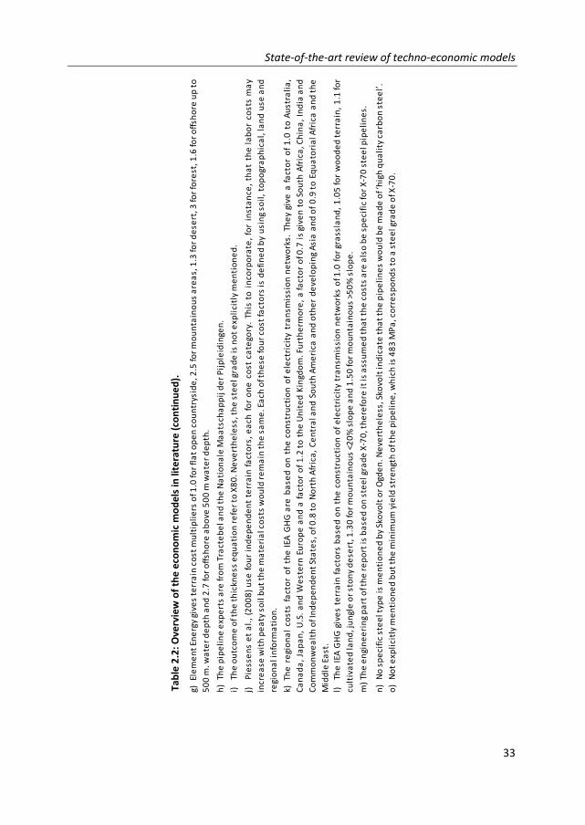
State‐of‐the‐art review of techno‐economic models
33
Table 2.2: O
verview of the economic m
odels in
literature (continued).
n) No specific steel type is mentioned by Skovolt or Ogden. N
evertheless, Skovolt indicate that the pipelines would be made of ‘high quality carbon steel’.
o) Not explicitly mentioned but the minim
um yield strength of the pipeline, w
hich is 483 MPa, corresponds to a steel grade of X
‐70.
h) The pipeline experts are from Tractebel and the Nationale Maatschappij der Pijpleidingen.
i) The outcome of the thickness equation refer to X80. N
evertheless, the steel grade is not explicitly mentioned.
j) Piessensetal.,(2008)use
fourindependentterrain
factors,each
foronecost
category.Thisto
incorporate,forinstance,thatthelaborcostsmay
increase
withpeatysoilbutthematerialcostswouldremainthesame.Each
ofthese
fourcostfactorsisdefinedbyusingsoil,topographical,landuse
and
regional inform
ation.
k) TheregionalcostsfactoroftheIEAGHGare
basedontheconstructionofelectricity
transm
issionnetw
orks.
Theygive
afactorof1.0
toAustralia,
Canada,Japan,U.S.andWestern
Europeandafactorof1.2to
theUnitedKingdom.Furtherm
ore,afactorof0.7
isgivento
South
Africa,China,Indiaand
CommonwealthofIndependentStates,of0.8to
NorthAfrica,CentralandSouth
America
andotherdevelopingAsiaandof0.9to
EquatorialAfricaandthe
Middle East.
l) TheIEAGHGgivesterrain
factors
basedontheconstructionofelectricity
transm
issionnetw
orksof1.0
forgrassland,1.05forwoodedterrain,1.1for
cultivated land, jungle or stony desert, 1.30 for mountainous <20% slope and 1.50 for mountainous >50% slope.
m) The engineering part of the report is based on steel grade X‐70, therefore it is assumed that the costs are also be specific for X‐70 steel pipelines.
g) Element Energy gives terrain cost multipliers of 1.0 for flat open countryside, 2.5 for mountainous areas, 1.3 for desert, 3
for forest, 1.6 for offshore up to
500 m. w
ater depth and 2.7 for offshore above
500 m
water depth.

Chapter 2
34
ElementEnergy (2010) derived a constant factor of 1,605 (± 642) €2010/m2 by a linear
regression of FERC cost data for pipelines with diameters of 0.76 and 0.91 m. It is not clear if the original data is corrected for inflation. The cost figure is only valid for pipelines on flat open countryside in developed countries, for other topographic conditions and regions, correction factors are used, see Table 2.2.
Models based on the weight of the pipeline (weight based models) 2.4.1.2
Gao et al., (2011) developed a cost model, which is specific for the Chinese market. However, with a few adaptations the model can easily be used for other parts of the world. The starting point of the model is the assumption that the cost of the pipeline is related to its weight (equation 2.2). This is used to determine the overall costs of the pipeline (equation 2.4).
0.02466 (2.2)
(2.3)
(2.4)
where, Wsteel is the weight of the steel pipeline (kg)9; OD is the outer diameter of
the pipeline (mm); L is the length of the pipeline (m); t is the wall thickness of the pipeline (mm)10; Pmax is the maximum operation pressure (15.3 MPa); S is the minimum yield stress (483 MPa); F is the design factor (0.72); E is the longitudinal joint factor (1); I refer to the total investment costs (€); Pp is the price of steel pipeline (€/kg) and fm is the fraction of material costs in the total pipeline costs.
Gao et al., (2011) indicate that the fraction of material costs (fm) is between 22 and 34% for the USA, and estimate this fraction to be 50% for the Chinese situation, due to lower labor costs. For the Chinese market, they use a price of pipeline X‐70 steel of 0.9 €/kg, based on data of a Chinese manufacturer of steel pipelines.11
Piessens et al., (2008) also use an equation for the required weight of steel multiplied by the steel price for analyzing the material costs of CO2 pipelines. To incorporate economies of scale for longer pipelines, an additional factor is incorporated (namely ‐16 x OD x ln (L) x L), see equation 2.5.12 However, this can cause strong economies of scale and even negative costs with long distances (1,000 km) and small diameters (0.01 m). To avoid negative costs and very strong economies of scale, the second part of the equation
9 The constant 0.02466 is derived by multiplying the density of steel (7,700 kg/Nm
3) by π and dividing it with 10
6
to get the right units (Fang, 2011). 10 The wall thickness is calculated by using the method specified in the USA code of federal regulation.
11 The RMB are converted to Euros with the exchange rate mentioned in (Gao et al., 2011), which is
8.6 RMB/€2010. 12 The equation in the source has an extra square after . However, it is confirmed by Piessens
that this is a typo mistake (Piessens, 2011). Hence, the square is removed from the equation.

State‐of‐the‐art review of techno‐economic models
35
(16 x OD x ln (L) x L) is restricted to become maximal 30% of the first part of the equation (L x St x FP x ( π x 7,850 / 4 ) x (OD2 ‐ (OD‐t)2)) (Piessens, 2011). For determining the total investment of CO2 pipelines, Piessens et al., (2008) also derive cost equations for labor, miscellaneous and ROW costs (equations 2.7‐2.9).
,16 (2.5)
. (2.6)
1,033 55.6 _ (2.7)
238 48 _ (2.8)
636 24 _ (2.9)
where, Ix refer to the investment costs of material (x=material), labor (x=labor), right‐to‐way (x=ROW) and miscellaneous (x=miscellaneous), respectively (€2010); L is the length (m); St are the steel costs (0.750 €2010/kg)
13; FP is the factor for regional steel product (about 8)14; OD is the outer diameter (m); t is the wall thickness of the pipeline (m); FT is the under thickness tolerance factor (0.125); Pave is the average transport pressure in the pipeline (9.5 MPa); S is the minimum yield stress (246 MPa); FC is the factor for threading, mechanical strength and corrosion (0.00127); and Fr_x is the correction factor for different regions for labor (x=labor), right‐to‐way (x=ROW) and miscellaneous (x=miscellaneous), respectively.
Note that the weight‐based models are the only models that explicitly incorporate thickness of the pipeline.
Quadratic equations 2.4.1.3
The IEA GHG report of 2002 analyzed the cost for the transmission of CO2 and energy, onshore as well as offshore. Six different kinds of coefficients are given for cost equation 2.10, for three different kinds of carbon steels, namely ANSI 600# (for pressures up to 9 MPa), 900# (up to 14 MPa) and 1500# (up to 22.5 MPa) for onshore as well as offshore (IEA GHG, 2002).15 ANSI 600# is considered not suitable for CO2 pipelines due to the small difference between the critical pressure and the maximal allowed pressure and is therefore not considered further. The cost equation of ANSI 1500# is used in an IEA GHG study for the construction of cost supply curves in Europe (Wildenborg et al., 2004).
13 The corrected steel price is slightly higher than the current steel price for hot rolled steel plate which was on
average 0.67 €2010/kg in the period August 2010 until September 2011 (Steelonthenet, 2012). 14 Factor of 8 is not stated in the article but is communicated by Piessens (Piessens, 2011).
15 ANSI is no longer used as standard and it has been taken over by the ASME standard. ASME give for straight
seam less pipes the recommendation to use the API standard (X70, X80 etc.). ANSI 1500# can still be found for flanges and valves, but this cannot be compared to the API pipeline standard.

Chapter 2
36
a (2.10)
where, I refer to the investment costs (M€2010); ai and bi are constants (for values see Annex A); L is the length (m); OD is the outer diameter (m); FT and FR are the correction factors for different terrains and for different regions, respectively.
In another study, Parker (2004) analyzed construction cost data on natural gas, oil and petroleum pipelines, and use the results to assess the costs for a hydrogen infrastructure. Although the aim of the study was not to look at CO2 infrastructure, the analysis has been used by several papers when assessing CO2 pipeline transport (McCollum and Ogden, 2006; Chandel et al., 2010). Parker (2004) developed a cost equation for each cost category (material, labor, ROW and miscellaneous costs), based on the best fit of the medians (equations 2.11‐2.14). For the period investigated, the average percentages of errors indicated by the author are 31% for material, 49% for labor, 59% for miscellaneous and 84% for ROW costs. Subsequently, Parker added the costs of each category to develop an equation for the total costs, which he estimates to have an average error percentage of 42% for the investigated period.16
489,160 25,827 25,743 53,785 (2.11)
507,661 77,969 162,341 284,294 (2.12)
21,691 28,444 61,469 (2.13)
316,425 6,994 145,989 (2.14)
996,820 441,912 223,522 545,537 (2.15)
where, D is the diameter (m); L is the length (km); and Ix refer to the investment costs of material (x=material), labor (x=labor), right‐to‐way (x=ROW), miscellaneous (x=miscellaneous), and total (x=total), respectively (€2010).
CMU model 2.4.1.4
McCoy and Rubin (2008) developed a cost equation for pipeline transport with different parameters for each cost category (material, labor, ROW and miscellaneous costs) and for each region, see equation 2.16. For the cost comparison in this article, the equations of the Mid‐West USA region are used, which corresponds to the base case in the article.
(2.16)
⋯ (2.17)
where, I refer to the total construction costs (€2010); L is the length (km); an are constants, which are specified for each cost category (see Annex A); D is the diameter (m); Xn are binary values for one of the 6 USA regions (see Annex A).
16 In the original formula for the total costs, a typo mistake was made in the last term. This was validated by
(McCollum and Ogden, 2006), who had contact with the author.

State‐of‐the‐art review of techno‐economic models
37
Models based on flow rates 2.4.1.5
For the construction of cost supply curves for CCS for North America, Dahowski et al., (2004) assumed that the costs for onshore CO2 pipelines have a linear relationship with length and diameter, see equation 2.1. A constant cost factor of 1,508 €2010/m
2 is used, which is obtained by linear regression of FERC cost data.17 Subsequently, Dahowski et al., (2004) rewrote the linear cost equation, which depends on diameter, by assuming that 1,000 million standard cubic feet per day is transported per square meter of pipe area to obtain an equation that only depends on flow and length, see equation 2.18. In the model, the distance between the source and sink is calculated as a straight line. However, since a pipeline will probably not be placed in a straight line to avoid, for example, densely populated areas and pipeline laying in other topographical conditions than flat, dry and remote grassland will add to the cost, the model incorporates an overall correction factor of 1.17. Additionally, a default amount of 10 miles (16 km) is added to the length to access a suitable injection site within a storage formation. However, in the comparison presented in this study, it is assumed that the actual length between source and sink is known and the cost comparison is done for pipelines on agricultural terrain, and consequently the correction factor and the default amount of 16 km are disregarded.
68,719 . (2.18)
where, I refer to the total investment costs pipeline (€2010); m is the mass flow (kg/s); and L is the length (km).
For constructing cost supply curves for CCS in China, the cost model of Dahowski et al., (2004) was updated (Dahowski et al., 2009). For the update, more recent FERC data was used and high and low cost outliers for each diameter category were excluded. The resulting cost equation is given in equation 2.19. Like in the originally model, a correction factor of 1.17 and a default amount of 40 km was used to correct for the straight line distance and the uncertainty where a suitable injection site is in the storage formation.18 For similar reasons as mentioned above, these were not taken into account in the comparison.
77,854 . 595,704 (2.19)
where, I refer to the total investment costs pipeline (€2010); m is the mass flow (kg/s); and L is the length (km).
In another study, Ogden et al., (2004) analyze the production chain of H2 production with CCS. The costs of CO2 transmission are based on the estimated investment cost of pipelines (including initial compression to 11 MPa) of 16, 30, 40 and 64 inches of Skovholt
17 It is not clear if the FERC costs are first adjusted for inflation, and if so to which base year. Therefore, the costs
are corrected by assuming that the costs are given in $2002, which is the last year of the data used from the FERC. 18 Since the spatial accuracy for CO2 point sources as well as for storage formations was less in China than in the
USA, a higher default amount of 40 km was used.

Chapter 2
38
(1993).19 With these data points, Ogden et al., (2004) derive an equation for the capital costs of pipelines (without initial compression) as function of the diameter. Subsequently, Ogden et al., (2004) reformulate the equation in such a way that the costs depend only on mass flow and length, see equation 2.20.
.
. (2.20)
where, C0 is the base costs per unit which 1,052 €2010/m; m is the mass flow (kg/s); L is the length (m); and subscript 0 refers to base case (L0 = 100,000 m; m0 = 185 kg/s).
Skovholt (1993) indicate that his cost estimations are applicable for onshore as well as offshore pipelines but excluded the extra compression costs for offshore transport. Ogden et al., (2004) focus only on onshore pipelines, so equation 2.20 is in this study only used for onshore pipelines.
McCollum and Ogden (2006) compare different existing economic models for CO2 transport in literature, namely the models of Ogden et al., (2004); Heddle et al., (2003); IEA GHG (2002); Wildenborg et al., (2004); Dahowski et al., (2004); and Parker (2004). Based on the average of these models a new cost model is proposed which eliminates the need to calculate the diameter, see equation 2.21.
24.7 . . (2.21)
where, I refer to the total investment costs onshore pipelines (€2010); m is the mass flow (kg/s) and L is the length (m).
Serpa et al., (2011) commence with the quadratic cost formula of the IEA GHG report of 2002, see equation 2.10. They note that the ratio between bi/ai is typically in the order of 10 (expressed in km). Therefore, they eliminate the b terms. Furthermore, the ratio between a2*OD
2 and a1*OD is higher than 5 for diameters above 0.50 m. Therefore, they simplify the equation by assuming that a1=0. Subsequently, they substitute OD for an equation containing the mass flow, resulting in equation 2.22.
(2.22)
∆ (2.23)
where, I refer to the investment cost (M€2010); a0 and a1 are constants; fdarcy is the Darcy friction factor; L is the length (km); ρ is the density (kg/m3); ΔP is the overall pressure drop (Pa); m is the mass flow of CO2 (Mt/y); γ is the exponent; and FT is the correction factor for different terrains.
To further simplify the equation, they assume that mass flow exponent γ is one instead of 0.8. To justify this simplification and to determine the values of a0 and β, they use several
19 The costs of Skovholt (1993) are directly used by Ogden et al., (2004) and not corrected for inflation.

State‐of‐the‐art review of techno‐economic models
39
cost estimations mentioned in public sources for CO2 and for large natural gas pipelines. With a linear regression on the cost data corrected to €2010, they found an a0 of 0.533 and a β of 0.019 with a R2 of 0.80 (Serpa et al., 2011).
Another study investigates the potential economies of scale of CO2 transport with a trunk pipeline (Chandel et al., 2010). They use the pipeline costs of Parker (2004) but only take into account pipelines with lengths longer than 75 miles (=120.7 km), because these are considered to be representative for long distance CO2 pipelines. For a given distance and mass flow, they calculate the needed diameter and round it up to a diameter that is commercially available. Subsequently, the amount of pumps needed on the route is calculated including one pump at the end of the pipeline to (re)pressurize the CO2.
20 With the capital costs, energy costs and O&M costs, the levelized costs are calculated for several mass flows and lengths. Based on the outcomes, a mass flow based equation is constructed for the levelized costs of CO2 transport, see equation 2.24.
..
. (2.24)
Where, L is the length (km); m is the mass flow of CO2 (kg/s); and LC refers to the levelized costs per t CO2 transported (€2010/t).
Models for O&M costs of pipelines 2.4.2
The majority of the levelized costs of CO2 pipeline transport consists of annualized capital cost but the O&M costs are nonetheless significant (McCoy and Rubin, 2008). In literature, the annual O&M costs for pipelines are generally expressed as a percentage of the capital costs, in the range of 1.5 to 4%, an equation, or expressed as a fixed value per unit length ranging from 4.5 to 7.0 €2010/m (see Table 2.3). No explanation is provided in literature for the different methods or for the range in the numbers.
Models for capital costs of pumping stations 2.4.3
For pumping stations less capital costs models are available than for pipelines. In total, five cost estimations for pumping stations were found in literature. Two studies used a relation between the capital cost and the installed capacity of the pumping station, namely the IEA GHG (2002), see equation 2.25, and Chandel et al., (2010), see equation 2.26.
12 0.71 10 (2.25)
2.3 0.15 10 (2.26)
where, Ipump refer to the investment costs of a pumping station (€2010) and W is the capacity of the pumping station (MWe)
20 In the article of Chandel et al., (2010) it is not clear why they place a pumping station at the end of the pipeline
to repressurize it back to the inlet pressure. Probably, the storage field requires this.

Chapter 2
40
Table 2.3: Overview of O&M costs for pipelines.
Model Onshore Offshore
ElementEnergy, 2010 1.5%a
3%a
Dahowski et al., 2004 2.0%a
Dahowski et al., 2009 2.5%a
Chandel et al., 2010 2.0%a
McCollum and Ogden, 2006 2.5%a
Wildenborg et al., 2004 3.0%a
Van den Broek et al., 2010b 3.5%a
Gao et al., 2011 4.0%a
Ogden et al., 2004 4.0%a
IEA GHG, 2002b ‐400,000+2,521xOD+2.7xL (154+19.8xL)x1000
Heddle et al., 2003 4,503 €2010/km/yMcCoy and Rubin, 2008 4,597 €2010/km/yZEP, 2011 6,240 €2010/km/yMikunda et al., 2011 7,000 €2010/km/yNETL, 2010 7,037 €2010/km/y
a) Annual O&M costs are based on a percentage of the capital costs.b) In the equations for O&M costs, OD is the outer diameter in millimeter, L is the length in meter and the O&M
costs are calculated in €2010. For the offshore O&M costs, a table is provided in the IEA report with the costs of intelligent pigging, a repair vessel and survey vessel. These are converted to an equation for the O&M cost, by assuming that surveying is executed each year and pigging speed is, like the surveying speed, 6 km/day. For offshore as well as for onshore O&M costs are similar for ANSI 900# and 1500#.
Additionally, ElementEnergy (2010) estimated the capital costs at 5 M€2010/MWe with an uncertainty range of 0.8‐8 M€2010/MWe. This includes associated infrastructure, land and standard levels of redundancy. It is not clear, however, where the numbers come from.
Piessens et al., (2008) and Wildenborg et al., (2004) reported fixed capital costs for pumping stations regardless the overall installed capacity. Piessens et al., (2008) reported capital costs of 38.6 M€2010 for the (intermediate) compressor, based on Wong (2005). 21
Wildenborg et al., (2004) estimated the costs on 10 M€2010 for a pumping station onshore, which is needed every 200 km. For the construction of cost supply curves of CCS for Europe, Wildenborg et al., (2004) used a fixed additional amount of 50 €2010/m to incorporate the costs of pumping stations also if the pipeline is shorter than 200 km. After the example of McCollum and Ogden (2006), this study incorporates only pumping station costs if pipelines are longer than 200 km.
Models for energy consumption, energy costs and fixed O&M costs of pumping 2.4.4stations
The O&M costs of pumping stations can be split in fixed O&M and energy costs. Fixed O&M costs are often expressed as a percentage of investment costs and are reported in the range of 1.5%‐5%, see Table 2.4. The energy costs, at the other hand, are related to the electricity price, operation hours and installed capacity. The IEA GHG (2002),
21 The original capital costs are given on a yearly basis (4.9 M€2010) but this can be converted to investment costs
using the given discount rate of 12% and the lifetime of 25 years.

State‐of‐the‐art review of techno‐economic models
41
ElementEnergy (2010), Chandel et al., (2010), Wildenborg et al., (2004) and McCollum and Ogden (2006) calculate the required installed capacity with the difference between the inlet and outlet pressure, see equation 2.27. Depending on the density, pressure in‐ and outlet, this leads to an energy consumption of 1.3– 4.5 kWh/t CO2, see Table 2.4.
(2.27)
where, W is the capacity of the pumping station (MWe); m is the mass flow (kg/s); ρ is the density (kg/m3); Pfinal is the pressure outlet pumping station (MPa); Pcut‐off is the pressure inlet pumping station (MPa); ηpump is the efficiency of the pump.
Piessens et al., (2008) derived the installed capacity from the difference in potential energy from the in‐ and out‐coming stream of the pumping station (see equation 2.28). They indicated that the energy consumption of compressing CO2 of 10°C from 8 to 13 MPa is 65 kWh/t CO2, if the compressor has an efficiency of 80%. The main reason for this large energy consumption is the temperature increase of almost 100°C, which is calculated with equation 2.29. However, this equation is only valid for adiabatic compression and not for pumping. With pumping, the temperature increase is considerably less. Therefore, the pumping process was modeled in AspenPlus by using the input data of Piessens et al. This leads to a temperature increase of only 1.5°C instead of 100°C. Furthermore, the energy consumption is about 7.2 kJ/kg or 2.0 kWh/t CO2. This figure is comparable with the range mentioned by the other authors, as can be seen in Table 2.4.
Table 2.4: Overview of O&M costs and energy consumption for pumping stations.
O&M costs Energy consumption (kWh/t CO2)
ElementEnergy, 2010 5%a
1.9b
Wildenborg et al., 2004 5%a
1.9b
IEA GHG, 2002c
N x (‐0.28W2 +1,033W + 244,788) 1.9
b
McCollum and Ogden, 2006 4%a
4.5d
Chandel et al., 2010 4%a
1.3e
Piessens et al., 2008 0.24 M€2010/y 2.0f
Van den Broek et al., 2010b 4‐5%a
n.a.Rubin et al., 2008 1.50%
a1.43
g
a) Percentage of investment costs. b) The energy consumption is calculated by using equation 2.25 and assuming an energy density of
800 kg/m3, an efficiency of 75% and a pressure difference of 4.0 MPa.
c) The O&M for pumps are originally based on a look up table (IEA GHG, 2002) but in the comparison the O&M equation developed by McCollum and Ogden is used, which has a R
2 of 0.93 for individual capacities
between 0‐2 MWe (McCollum and Ogden, 2006). In the formula, N is the number of pumping stations, W the capacity in kWe and the O&M costs are given in €2010.
d) McCollum and Ogden (2006) also use equation 2.25 but they assume a density of 630 kg/m3, an efficiency
of 75%, an inlet pressure of 7.38 MPa and an outlet pressure of 15 MPa. e) Also, Chandel et al., use equation 2.25 but they use a density of 827 kg/m3
, an efficiency of 75% and a pressure difference of 3 MPa.
f) Piessens et al., (2008) give an energy consumption figure of 65 kWh/t CO2 for pumping CO2 of 10°C from 8 to 13 MPa. This is, however, related to a temperature increase of 100°C between the inlet and outlet while with pumping the temperature increase is only 1.5°C. Looking up the difference in internal energy of this gives a difference in internal energy of 7.2 kJ/kg, which correspond to an energy consumption of 2.0 kWh/t CO2 with an pump efficiency of 80%.
g) Estimated compression power for pumping CO2 of 12°C from 10 to 14 MPa (Rubin et al., 2008).

Chapter 2
42
, , (2.28)
(2.29)
where, W is the power (kW); Ep,1‐2 is the potential energy of state 1 and 2, respectively (kJ/kg); m is the mass flow (kg/s); ηpump is the efficiency of the pump; Toutlet is the outlet temperature; Tinlet is the inlet temperature; CR is the compression ratio between outlet and inlet22; k is the ratio between cp and cv; cp is the specific heat of CO2 under constant pressure kJ/(kg*K)23; and cv is the specific heat of CO2 under constant volume kJ/(kg*K)24.
Evaluating the economic pipeline and pumping station cost 2.5models
In this section, the pipeline and pumping stations cost models are compared with each other. If correction factors are included in the cost formulas to distinguish between different topographic and regional conditions, the factors are set to 1, corresponding to costs of onshore pipelines on flat terrain.
Evaluation of pipeline cost models 2.5.1
Figure 2.3 shows a comparison of the different capital costs models over a range of diameters. The model of Piessens et al., (2008) results in significantly higher capital costs than the other models. The main reason for this is the material costs, which determine up to 88% of the total costs for large diameters in their model. This is caused by the increasing wall thickness, which goes from 5 to 30 mm if the diameter increase from 0.20 to 1.30 m.25 This leads to a 39‐fold increase in steel requirements. For Gao et al., (2011) the cost consequence of the higher steel requirement is less strong due to the assumed lower costs for steel pipelines.
Even without the cost estimation of Piessens et al., (2008) the cost difference between the lowest estimation and the second highest is large. For instance, for a diameter of 0.4 m the cost difference between the estimation of Van den Broek et al., (2010a) and IEA GHG (2002) for ANSI #900 is a 0.5 M€2010/km, equivalent to almost a 150% cost difference.
In Figure 2.3, costs estimations are included of existing (Weyburn, Kinder Morgan and
22 To pressurize CO2 from atmospheric pressure to, for instance, 10 MPa, multiple stages are installed with
intercoolers between the stages to limit temperature increase. 23 The specific heat under constant pressure of CO2 depends on the pressure and temperature. For instance, CO2
with a pressure of 10 MPa and a temperature of 280 K, has a specific heat of 2.28 kJ/(kg*K) (Span and Wagner, 1996). 24 The specific heat under constant volume of CO2 depends on the pressure and temperature. For instance, CO2
with a pressure of 10 MPa and a temperature of 280 K, has a specific heat of 0.93 kJ/(kg*K) (Span and Wagner, 1996). 25 The thickness calculation is based on equation 2.6 and parameters of Piessens et al., (2008).

State‐of‐the‐art review of techno‐economic models
43
Denbury) and planned (Alberta Carbon Trunk and Kingsnorth) CO2 pipelines as well as costs estimations made in literature (Damen et al., 2009; Essandoh‐Yeddu and Gülen, 2009; WorleyParsons and EcoNomics, 2009; ZEP, 2010; Mikunda et al., 2011), see Annex A for the actual data. After correcting the cost models to the actual length of the realized and planned pipelines, the majority of the estimations are within the range indicated by the different costs models. Only one of the 39 data points was outside the range, namely the realized Centerline. For this pipeline the costs are estimated at 0.23 M€2010/km (Kinder Morgan Energy Partner, L.P., 2003), while the cost models give a range of 0.28 – 1.7 M€2010/km for a pipeline with a diameter of 0.41 m and a length of 182 km.26
Figure 2.3: Capital costs predicted by the different diameter based models in M€2010/km for a pipeline of 25 km on flat agricultural terrain and capital cost estimations in literature, for actual planned or realized projects (including terrain aspects).
27 The boxes represent the ranges for the different base cases resulting from the different diameter models (see section 2.6).
Denbury’s Green transverses through an area with large rivers, creeks, wetlands, highways and along a number of cities (Greenwell, 2010). To pass these problem areas, 69 horizontal drillings were executed for the pipeline while major projects have typically only 10‐15 drilling (Greenwell, 2010). This large number of drillings increased the costs considerably compared to a pipeline through agricultural land without any obstacle. The costs of the Green pipeline of about 1.1 M€/km are at the upper end of the range indicated by the different cost models, only the model of Piessens et al., (2008) and the model of Van den Broek et al., (2010a) give higher costs per km. These kind of
26 The cost range for the models is calculated by using the actual length of the pipeline.
27 The y‐axis is limited to 8.0 M€2010/km for clarity reasons. Therefore, the costs of Piessens et al., are not figured
for diameters above 0.85 m. According to Piessens et al., a pipeline with a diameter of 1.30 m and a length of 25 km costs 14 M€2010/km.
DEMO
COM
TRUNK
0.0
1.0
2.0
3.0
4.0
5.0
6.0
7.0
8.0
0.10 0.20 0.30 0.40 0.50 0.60 0.70 0.80 0.90 1.00 1.10 1.20 1.30
Costs (M
€2010/km)
Outer diameter (m)
Parker et al., 2004
Broek et al., 2010
Heddle et al., 2003
ElementEnergy, 2010
Gao et al., 2011
Piessens et al., 2008
IEA GHG, 2002. ANSI 900#
IEA GHG, 2002. ANSI 1500#
McCoy and Rubin, 2008
ZEP onshore
Wordley Parsons
Other sources
Alberta Carbon Trunk line
Kingsnorth CCS
Kinder Morgan
Weyburn
Denbury

Chapter 2
44
topographical factors can only to a limited extent be accurately covered by the cost models.
Figure 2.4: Capital costs of mass flow based models for a length of 25 km and 300 km on flat agricultural terrain and capital cost estimations in literature, for planned or realized projects (including terrain aspects).
28
28The mass flow based model of Chandel et al., gives the levelized costs of CO2 transport instead of capital costs.
To convert the levelized costs back to capital costs, a similar discount rate and lifetime is used as by Chandel et al., which is a discount rate of 10% and a lifetime of 25 years. There is corrected for the O&M costs of the pipeline, but not for the capital, energy and O&M costs of the pumping stations, because it is unknown how much pumping stations are installed. This will lead to a slightly overestimation of the capital costs, especially for larger distances.
DEMOCOM
TRUNK
0.0
0.5
1.0
1.5
2.0
2.5
3.0
0 50
100
150
200
250
300
350
400
450
500
550
600
650
700
750
800
Costs (M
€2010/km)
Mass flow (kg/s)
25 km Ogden, 2004
McCollum & Ogden, 2006
Serpa et al., 2011
Dahowski et al., 2005
Dahowski et al., 2009
Chandel et al., 2010
ZEP onshore
Other sources
Alberta Carbon Trunk line
Kingsnorth CCS
Kinder Morgan
Denbury
Weyburn
DEMO
COM
TRUNK
0.0
0.5
1.0
1.5
2.0
2.5
3.0
0 50
100
150
200
250
300
350
400
450
500
550
600
650
700
750
800
Costs (M
€2010/km)
Mass flow (kg/s)
300 km Ogden, 2004
McCollum & Ogden, 2006
Serpa et al., 2011
Dahowski et al., 2005
Dahowski et al., 2009
Chandel et al., 2010
ZEP onshore
Other sources
Alberta Carbon Trunk line
Kingsnorth CCS
Kinder Morgan
Denbury
Weyburn

State‐of‐the‐art review of techno‐economic models
45
The capital cost estimations for the mass flow models are given in Figure 2.4. With a distance of 25 km, the cost estimation of McCollum and Ogden (2006) is always the lowest from the analyzed mass‐flow based models. The model of Chandel et al., (2010) gives the highest cost estimation for mass flows of 550 kg/s and more. For lower mass flows, the model of Dahowski et al., (2004) give the highest estimations. Note that the updated model of Dahowski et al., (2009) give lower estimations than the originally model, which can be caused by the exclusion of low and high cost outliners in the updated model. For very small mass flows of 75 kg/s and less, the model of Serpa et al., (2011) provides the lowest costs. If the distance increases to 300 km, the costs estimated from McCollum and Ogden (2006) and Ogden et al., (2004) increase with 40% and 80%, respectively. As a consequence, the cost estimated by Ogden et al., (2004) are the highest for all base cases. Reasons for this specific cost increase are not provided.
After correcting the mass flow based models to the right length, five of the 22 cost estimations from realized or planned CO2 pipelines or estimations made in literature, are outside the cost range indicated by the models. Namely:
‐ The costs estimation of the realized Weyburn pipeline of 0.48 M€2010/km is below the indicated range of the mass flow based models of 0.50 – 1.1 M€2010/km for a pipeline with a capacity of 95 kg/s and a length of 328 km (Dakota Gasification Company, 2011; IEA GHG, 2011);
‐ The cost estimation of a realized Centerline of 0.23 M€2010/km is below the indicated range of 0.63 – 1.5M€2010/km for a pipeline with a design capacity of 175 kg/s and a length of 182 km (Kinder Morgan Energy Partner, 2003);
‐ The cost estimation of the Eastern Shelf CO2 pipeline of 0.20 M€2010/km is below the indicated range of 0.55 – 1.2 M€2010/km for a pipeline with a capacity of 120 kg/s and a length of 146 km (Bradley, 2011; Kinder Morgan, 2011);
‐ The highest cost estimation for Kingsnorth, which is a planned CO2 pipeline with a capacity of 304 kg/s and a length of 278 km for a CCS demonstration project in the United Kingdom, is 2.5 M€2010/km and above the indicated range of 0.72 –1.9 M€2010/km. However, the majority of this pipeline will be offshore which will increase the construction costs (EON UK, 2011ab).
‐ The cost estimation of 1.2 M€2010/km for a pipeline in Europe made in literature is above the indicated range of 0.38 –1.1 M€2010/km for a CO2 pipeline with a capacity of 79 kg/s and a length of 10 km (ZEP, 2010). A possible reason for this is the limited length of the pipeline.
The main advantage of the mass flow based models is that it is not necessary to calculate the diameter. However, it is difficult to see what kind of assumptions behind pressure inlet, pressure drop, temperature, distance between pumping stations, roughness height etc. are made. Consequently, the flexibility to adapt the design to certain circumstances is reduced. For instance, it is not possible to adapt the model to a different inlet or outlet pressure or for height differences.

Chapter 2
46
Regional differences 2.5.2
Several sources indicate that also regional circumstances influence overall pipeline costs, mainly due to differences in labor costs (IEA GHG, 2002; Gao et al., 2011; Serpa et al., 2011). Therefore, regional correction factors are used by the IEA GHG (2002), based on electricity transmission networks, and ElementEnergy (2010).29 They both indicate that the costs in Western Europe are similar as in the USA. However, another source indicate that energy technologies are 10% more expensive in Western Europe than in the USA (IEA, 2008). To assess whether pipeline costs from America pipelines can be used as approximation for the European market or for other parts of the world, cost data for recent natural gas pipelines or planned natural gas pipelines in Europe and other parts of the world in the period 1993‐2011 are compared to U.S. FERC data for the period 1994‐2010.30,31
In the U.S., there is an abundance of pipeline costs data due to regulation requirements. However, for Europe and other parts of the world, this is not the case and only a limited amount of data was found and then especially for large projects. In Figure 2.5, the cost estimations are given ordered by diameter (A), by length (B) and by length for one specific diameter (C).32 It can be seen that there is one pipeline from other countries which has very high specific costs of about 12 M€2010/km. This specific pipeline is realized in Russia in an area with very difficult topographic and climate conditions, which increased the costs. Furthermore, it becomes clear from Figure 2.5A, that there is a large variation in costs per kilometer for a given diameter. Economies of scale is partly an explanation for this variation (Figure 2.5B), especially pipelines with a short length (< 10 km) seems to have high specific costs. To see more clearly the impact of length without the disturbance of diameter, the specific costs for a specific diameter of 0.91 m (chosen because for this diameter most cost data was available) are given in Figure 2.5C.
To see if there are significant differences between the median of the specific costs of the three regions, a Kruskal‐Wallis analysis was conducted to the specific costs of pipelines the U.S., Europe and other countries.33 This analysis showed that there are no significant
29 Although it is not stated, it seems to be that ElementEnergy (2010) based their regional correction factors on
the (IEA GHG, 2002). 30 The U.S. cost data is based on FERC data from 1994‐2011 (True, 1995; True, 1996; True, 1997; True, 1998;
True, 1999; True, 2000; True, 2001; True, 2002; True, 2003; True and Stell, 2004; Smith, 2006; Smith, 2007; Smith, 2008; Smith, 2009; Smith, 2010; Smith, 2011). 31 Cost data for pipelines in Europe and other countries come from different sources (Editorial staff, 1993; Pitt,
2008; Wingas Transport, 2008; Cronenberg et al., 2009; Kampman et al., 2010; Ministry of Petroleum, 2010; PPIAF, 2010; Gasunie, 2011; Gazprom, 2011; Hydrocarbons‐technology, 2011abcdef; NEL‐pipeline, 2011; OPAL‐pipeline, 2011; Petrova, 2011; Reuters, 2011; Serpa et al., 2011; Smith, 2011; Wikipedia, 2011; Money Express, 2012; PennEnergy, 1998). An overview of the actual data is given in the Annex A. 32 In the data, there was one extreme cost outliner for U.S. pipeline which is not visible in the graph. This was a
pipeline with a diameter of 0.61 m, a length of 0.02 km leading to average costs of 23 M€2010/km. 33 The Kruskal‐Wallis analysis was chosen because it can deal with the unequal variance of the different groups
and with the very different sample size of 327 for U.S., 20 for Europe and 16 for other countries.

State‐of‐the‐art review of techno‐economic models
47
02468
10
12
14
01
10
100
1.00010.000
Costs (M€2010/km)
Length (km
)
B.
USA
Europe
Other countries
02468
10
12
14
0.1
0.3
0.5
0.7
0.9
1.1
1.3
1.5
Costs (M€2010/km)
Diameter (m
)
A.
USA
Europe
Other countries
02468
10
12
14
01
10
100
1.000
Costs (M€2010/km)
Length (km
)
C.
USA
Other countries
Figure 2.5: Specific costs for natural gas pipelin
es ordered by (A) diameter, (B) length and (C) length for a specific diameter of
0.91m.

Chapter 2
48
differences in the median between U.S., Europe and other countries (p=0.77). Note that this analysis excludes the effect of diameter and length. Overall it has been concluded that possible regional cost differences are masked in the large cost range.
Analysis of results for pipeline capital costs 2.5.3
Although all pipeline costs models have length as one of the key variables, the effect of doubling the pipeline length on the cost differs. For instance, the linear models of Heddle et al., (2003); ElementEnergy (2010); and Van den Broek et al., (2010a), the weight model of Gao et al., (2011) and the flow rate models of Dahowski et al., (2004), Chandel et al., (2010) and Serpa et al., (2011) assume a linear relation with respect to length. So, doubling the pipeline lengths results in a doubling of the total costs. Looking to the original FERC data (see Figure 2.5), it can be seen that it is likely that the specific costs decrease considerably if the length of the pipeline doubles from 5 to 10 km. However, after the pipeline has reached a certain length, about 50 km, strong additional economies of scale are not likely to be realized when the pipeline becomes longer.
Other models assume economies of scale related to length, namely the model of Piessens et al., (2008), the quadratic equations (IEA GHG, 2002; Parker, 2004), the CMU model (McCoy and Rubin, 2008) and the flow rate model of Dahowski et al., (2009). Piessens et al., (2008) incorporate economies of scale for labor, material and miscellaneous costs. For ROW costs, on the other hand, Piessens et al., (2008) assume a linear relationship but this is only a small part in the overall costs. The realized economies of scale depend on the actual length and diameter of the pipeline, for instance doubling the length of a pipeline of 300 km with a diameter of 0.5 m gives a 2.5% cost advantage. In the quadratic equations, the effect of the overall constant becomes smaller as the pipeline becomes longer. This gives, for instance, a costs advantage of approximately 1% when the pipeline length is doubled from 300 to 600 km. In the CMU model, the factor La is incorporated where ‘a’ is in all cases, except for the ROW costs, smaller than 1 (McCoy and Rubin, 2008). Overall, the specific costs decrease by approximately 10% when the length of the pipeline is doubled. In the flow rate model of Dahowski et al., (2009), the constant of 0.6 M€ creates minor economies of scale related to length of about 1% if the pipeline length doubles from 25 to 50 km. For longer lengths, it can be better considered as a linear model.
Two models imply reverse economies of scale related to length, meaning that the specific pipeline cost increase as the pipeline gets longer. The specific costs increase by 9.4% and 18% when the pipeline is doubled in the mass flow based model of McCollum and Ogden (2006) and Ogden et al., (2004), respectively. Reasons for this are not provided in literature.
For all models, which include diameter as variable, a larger diameter leads to higher costs but different relations can be observed. Doubling the diameter from 0.4 to 0.8 m results in two times higher investment costs for the linear cost models. For the CMU, quadratic and the weight based models, the costs more than double. For the model of Gao et al., (2011) the largest cost increase is observed if the pipeline diameter is doubled, namely a 3.8 fold

State‐of‐the‐art review of techno‐economic models
49
cost increase. This is immediately related to the amount of steel needed, which doubles due to the larger circumference and increase with 188% due to the estimated thicker wall. Since Gao et al., (2011) assume that the material costs are always 50% of the total costs, they indirectly assume that also the labor, miscellaneous and ROW costs will increase a 3.8‐fold when the diameter doubles. Looking to the FERC data (Figure 2.5), it can be seen that the total specific costs increase with a factor 2 ‐ 2.5 if the diameter doubles. Zooming in shows that the material cost approximately triple, the labor costs more or less double, the ROW costs remain almost constant and the miscellaneous costs increase to a minor extent.
Wall thickness is strongly influenced by the maximum operation pressure and the steel grade used. A doubling in operation pressure would approximately double the required thickness. If steel grade X80 instead of X70 is used, for instance, the wall thickness is reduced by 2.5 mm to 18 mm for a pipeline diameter of 1.22 m (Gräf et al., 2003). Besides influencing the wall thickness and material costs, the steel grade will also affect construction costs, because transportation costs are reduced and thinner walls are easier to weld (Gräf et al., 2003). The lower construction costs and lower amount of steel required, more than compensate the higher material costs per kilogram steel, and overall a cost reduction between 3.5 and 30% is estimated if X100 instead of X70 is used (Sanderson et al., 1999; Gräf et al., 2003; Cayrade, 2004; Felber and Loibnegger, 2009). Despite the large influence of steel grade on the design and costs of the pipeline, only three sources (IEA GHG, 2002; Gao et al., 2011; Serpa et al., 2011) explicitly mention the steel grade of their cost models. The other sources do not mention this and use FERC data as basis for the costs equations.
In addition, all models, except the weight‐based models, do not incorporate directly a steel or iron price, which increased considerably during the last few years (see Figure 2.6). A doubling in steel price will increase the total construction costs of pipelines by approximately 20‐35%. Although increasing material prices are included in cost indexes, like the UCCI, it is almost impossible to determine whether the steel intensity of the products included in the index is comparable to pipelines. Therefore, it would be more accurate to link the material prices of the pipeline directly to the steel price or a steel price index.
Analysis of results for pipeline O&M costs 2.5.4
Most of the sources give O&M costs as a percentage of the capital costs of the pipeline, which range from 1.5% to 4.0% (Dahowski et al., 2004; Ogden et al., 2004; Wildenborg et al., 2004; McCollum and Ogden, 2006; Chandel et al., 2010; ElementEnergy, 2010; Van den Broek et al., 2010a; Gao et al., 2011). However, the spread in capital costs is large, as Figure 2.3 and Figure 2.4 show, and therefore, the actual O&M costs vary even more.
Other studies use a fixed amount for the O&M costs regardless the diameter, namely (Heddle et al., 2003; McCoy and Rubin, 2008; NETL, 2010; ZEP, 2010; Mikunda et al., 2011). Furthermore, one study (IEA GHG, 2002), derived a linear formula for the O&M costs. With this formula, strong economies of scale are realized, for instance, for a fixed

Chapter 2
50
diameter of 0.5 m the O&M costs are 42 €/m for a pipeline of 25 km and 6 €/m for 300 km. Figure 2.7 shows a comparison of the different O&M cost models. It can be concluded that models which use a fixed percentage give significantly higher O&M costs than models which use a fixed amount per kilometer for pipelines with large diameters.
Figure 2.6: World iron ore price from January 2001 until 2011 (Steelonthenet, 2011).34
Figure 2.7: Overview of the O&M costs predicted by the different models for a pipeline of 25 km on flat agricultural terrain.35 The boxes represent the ranges for the different base cases resulting from the different diameter models (see section 6).
34 World iron prices are corrected with the inflation index.
35 Chandel et al., give capital costs for fixed diameters, namely 0.39, 0.49, 0.59, 0.73, 0.88, 1.03 and 1.27 m
(Chandel et al., 2010). Hence, the O&M costs can only be given for these diameters.
0
10
20
30
40
50
60
70
80
90
100
Jan‐01
Jan‐02
Jan‐03
Jan‐04
Jan‐05
Jan‐06
Jan‐07
Jan‐08
Jan‐09
Jan‐10
Jan‐11
€2010/tonne
Iron ore price
Average
COM
DEMO
TRUNK
0
20
40
60
80
100
120
140
160
0.10
0.20
0.30
0.40
0.50
0.60
0.70
0.80
0.90
1.00
1.10
1.20
1.30
Costs (k€2010/km)
Outer diameter (m)
Broek et al., 2010
Heddle et al., 2003
ElementEnergy, 2010
Gao et al., 2011
ZEP, 2011
Mikunda et al., 2011
IEA GHG, 2002
NETL, 2007
McCoy and Rubin, 2008
Chandel et al., 2010

State‐of‐the‐art review of techno‐economic models
51
Analysis of results for the capital cost models of pumping station 2.5.5
The different capital cost models for pumping stations are compared with each other in Figure 2.8. There is a wide range in pumping station costs, for instance, the costs for a pumping station of 1.25 MWe are reported in the range 3.1‐36 M€2010.
36 The lowest cost estimation is based on Chandel et al., (2010) which use costs of initial pumps attached to a facility as an approximation for standalone pump. However, a standalone pumping station would be more expensive because infrastructure and buildings have to be constructed. For capacities under 3.0 MWe, the highest cost estimation is from Piessens et al., (2008) which use the costs of initial compression as approximation of pumping stations. However, the costs for compressing are considerably higher than for only pumping (IEA GHG, 2002; McCollum and Ogden, 2006). For larger capacities, the model of IEA GHG, (2002) predicts the highest costs for pumps.
ElementEnergy, (2010) assumes a linear behavior between capacity and costs, while all the other cost models include economies of scale. For the models of Chandel et al., (2010) and the IEA GHG (2002) the influence of the constant become smaller if the capacity increase. For instance, if the capacity doubles from 1.25 to 2.5 MWe the specific investment costs decline by 4‐5%. The other two models (Piessens et al., (2008) and Wildenborg et al., (2004)) assume a perfect inelastic cost behavior, meaning that total cost remains the same if the capacity changes. This seems unrealistic because the pump will increase significantly in size when the mass flow increases.
Figure 2.8: Capital cost of pumping stations from the different models. The boxes represent the ranges for the different base cases resulting from the different energy consumption figures for pumping.
36 Based on equation 2.25, a capacity of 1.25 MWe would be the required capacity to pump a COM mass flow of
150 kg/s with 5 MPa if the pump has an efficiency of 75% and the CO2 flow a density of 800 kg/m3. Using the
same equation and parameters, the capacities of DEMO and TRUNK would be 0.42 and 6.25 MWe, respectively.
COMDEMO
TRUNK
0
20
40
60
80
100
120
140
160
180
0 1 2 3 4 5 6 7 8 9 10
11
12
13
Costs (M
€2010)
Capcity (MWe)
Piessens et al., 2008
Wildenborg et al., 2004
Chandel et al., 2008
ElementEnergy, 2010
IEA GHG, 2002

Chapter 2
52
Analysis of results for O&M costs, energy consumption and levelized costs for 2.5.6pumping stations
The fixed O&M costs for pumping stations are most often given as a percentage of the capital costs, ranging from 1.5‐5.0% (Wildenborg et al., 2004; Rubin et al., 2008; Kazmierczak et al., 2009; Chandel et al., 2010; ElementEnergy, 2010; Van den Broek et al., 2010a). A different approach is taken by Piessens et al., (2008) which give besides fixed capital costs also a fixed amount of O&M costs, comparable to an O&M percentage of 1.0%. Furthermore, the IEA GHG (2002) provides a table with different O&M costs. These costs are translated into a formula by McCollum and Ogden (2006) for pumping stations up to 2 MWe. By comparing the different models with each other, see Figure 2.8, it can be concluded that the O&M costs of the IEA GHG are significantly higher than the other sources for capacities up to 2 MWe.
Like the O&M costs for pipelines, the fixed O&M costs for pumping stations are strongly influenced by the variation in capital costs (Figure 2.8). Consequently, the cost range would be even larger than depicted in Figure 2.9. For instance, the highest costs estimation for a pumping station of 1.25 MWe is 36 M€2010, multiplying this by the highest O&M cost percentage (5%), leads to fixed O&M costs of 1.8 M€2010/y. Similar the lowest O&M cost estimation for a 1.25 MWe pumping station is (3.1 x 1.5%=) 0.05 M€2010/y.
Besides fixed O&M costs, the pumping station will have associated energy costs. Piessens et al., (2008) estimate these on 2.4 M€2010/y, regardless the installed capacity. The other sources calculate the energy costs with a capacity factor (ranging from 80‐100%), installed
Figure 2.9: O&M costs of pumping station from the different models.37 The boxes represent the ranges for the different base cases resulting from the different energy consumption figures for pumping.
37 The formula derived by McCollum and Ogden for the O&M costs given in a look‐up table of the IEA GHG 2002
is only applicable for capacities until 2 MWe.
DEMO
COM
TRUNK
0.0
0.5
1.0
1.5
2.0
2.5
0 1 2 3 4 5 6 7 8 9 10
11
12
13
O&M costs (M
€2010/y)
Capacity (MWe)
Piessens et al., 2008
Wildenborg et al., 2004
Chandel et al., 2010
IEA GHG, 2002
Rubin et al., 2008

State‐of‐the‐art review of techno‐economic models
53
capacity and electricity costs (ranging from 34‐48 €2010/MWh). The installed capacity is directly related to the energy consumption needed which range from 1.3‐4.5 kWh/t CO2. However, the majority of the range is related to difference in input parameters like the in‐ and outlet pressure and density. Nevertheless, applying the range in energy consumption figures to calculate the installed capacity gives a capacity range of 0.2‐0.8 MWe for DEMO, 0.7‐2.4 MWe for COM and 3.6‐12 MWe for TRUNK. These ranges are also depicted in Figure 2.8 and 2.9.
With the capital, fixed O&M and energy costs, the levelized costs are calculated for a COM mass flow with a common energy price (50 €/MWh), capacity factor (95%) and capital recovery factor (15%). The results of this are given in Table 2.5. It can be concluded that the levelized costs vary considerably between the different sources from 0.16 to 1.9 €/t CO2. Moreover, the cost division varies significantly. For the model of McCollum and Ogden (2006), and to lesser extent of Chandel et al., (2010) the energy costs represent the largest share of pumping costs. However, Piessens et al., (2008), IEA GHG (2002) and Wildenborg et al., (2004) estimate that capital has the largest share in the costs. Additional, Piessens et al., (2008) and McCollum and Ogden (2006) estimate that the O&M costs are only a minor share of the total costs while Chandel et al., (2010) estimate it on almost one third.
For larger mass flow, the cost division of ElementEnergy (2010) and Piessens et al., (2008) does not change at all and some small changes arise with the models of Chandel et al., (2010) and McCollum and Ogden, (2006). However, in the model of Wildenborg et al., (2004) the share of capital costs decrease from 51% to 27% if a TRUNK instead of a COM flow is pumped. For the IEA GHG model, the share of capital costs increase, at expensive of the O&M costs, for larger mass flows.
Table 2.5: Levelized cost of pumping a COM flow, with a common capacity factor, capital recovery factor and energy price.
Review of pipeline diameter models applied in literature 2.6
Except for the models of Dahowski et al., (2009), Dahowski et al., (2004), Ogden et al., (2004), McCollum and Ogden (2006), Serpa et al., (2011) and Chandel et al., (2010) all pipeline cost models depend on the diameter rather than on mass flow. Therefore, it is useful to have insights into the key underlying parameters and assumptions which influence the diameter calculation and consequently the capital costs.
In literature, several different models are used or proposed to calculate pipeline diameter for CO2 transport. A brief overview of the different models is given in Table 2.6.
Share in levelized costs Levelized costs (€2010/tCO2)
Capital O&M Energy
ElementEnergy, 2010 43% 21% 36% 0.26Wildenborg et al., 2004 52% 26% 22% 0.42IEA GHG, 2002
54% 28% 18% 0.52
McCollum and Ogden, 2006 23% 9% 67% 0.33Chandel et al., 2010 26% 31% 43% 0.16Piessens et al., 2008 54% 3% 43% 1.9

Chapter 2
54
Table 2.6: O
verview of the different diameter calculation m
ethods in literature.
Nam
eForm
ula
Abbreviations
Sources
D = Diameter (m
)
m = Mass flow (kg/s)
v = Velocit y (m
/s)a
ρ = Density (kg/m
3)
f = Fanning friction factor
L = Length (m
)
ΔP = Overall pressure drop (Pa)
n = Manning friction factorb
Δh = Height difference
(m)
g = Gravity constant (9.81 m/s
2)
Z ave = Average
fluid compressibilityc
R = Gas constant (8.31 Pa*m
3/m
ol*K)
T ave = Average
fluid temperature (K)
M = M
olecular weight of flow (kg/km
ol)
P1 = Pressure at inlet (Pa)
P2 = Pressure at outlet (Pa)
Pave = Average
pressure in
the pipelinec
G = Specific gravity ( 1.519)
ηpipe = Pipeline efficiency (assumed to
be1)
a1 = Constant 1 (= 73.06)
a2 = Constant 2 (= 0.06836)
Velocity
based
equation
Wildenborg et al., 2004;
Kazm
ierczak et al., 2009;
ElementEnergy, 2010;
Chandel et al., 2010
Hydraulic
equation
Heddle et al., 2003; Van
den Broek et al., 2010b
Extensive
hydraulic
equation
Piessens et al., 2008
McCoy and
Rubin
model
McCoy and Rubin, 2008
Model of
Ogden et al.,
Ogden et al., 2004
a) Themostcosteffectivevelocityfordense
phase
CO2transportisestim
atedfrom1.5‐2.0
m/s(ElementEnergy,2010)to2‐4m/s
(Ogdenetal.,2004).
Chandel et al., pointed out that the actual velocity (v
act) can be lower than the design
velocity if the pipeline is not fully occupied.
b) Piessensetal.,adaptedthehydraulicequationto
incorporate
theeffect
ofheightdifference
andlocallossescausedbybendsin
thepipeline
(Piessens et al., 2008). For a fair comparison, the local losses are not taken into account in this analysis.
4ρ
π
32 π
ρΔ
4 πρ
ΔΔ ρ
64
π2
Δ
2 3
η
1000
1000
1000
Δ

State‐of‐the‐art review of techno‐economic models
55
The velocity based model is often used for an initial estimation of the diameter and not for a detailed design. The (extensive) hydraulic equation is only applicable for fluid transport while the model of McCoy and Rubin and the model of Ogden can be used for gaseous as well as for liquid transport. For an extensive overview and comparison we refer to Piessens et al., (2008). The different parameters used by the different models for pure CO2 transport are reported in Table 2.7.
Comparison of diameter models 2.6.1
The diameter models are compared with each other for a common mass flow, pipeline length and height difference but using the friction factor, velocity, temperature, density, in‐ and outlet pressure, and specific pressure drop of the sources (Table 2.7). Figure 2.10 shows a comparison of diameter for different mass flows for a transportation distance of 25 and 300 km. Three models (McCoy and Rubin, 2008; Piessens et al., 2008; Chandel et al., 2010) mention that only specific pipeline diameters are commonly available, and therefore they round the diameter up to the nearest nominal pipe size. This explains the stepwise increase in diameter shown in the figure. For COM‐25, the diameters range from 0.28‐0.41 m, which is a difference of more than 45% between the lowest and highest value. If the distance is increased from 25 to 300 km, the diameter range does not change much, see Table 2.8. However, the diameter calculated by some particular models change significantly. For instance, the diameter for a DEMO mass flow increases from 0.22 to 0.32 m if the distance is increased from 25 to 300 km in the model of McCoy and Rubin (2008).
The capital and levelized cost implications for the diameter ranges are given in Table 2.8, which are also depicted in Figure 2.3 and Figure 2.7. Overall, the difference between the highest and lowest cost estimation is a factor ten for all base cases.
In the previous analysis, the inlet and outlet pressure which is given in the sources was used for calculating the diameter. In fact, this leads to slightly different pipeline configuration but this reflects the uncertainty in the optimal configuration. For a given pipeline configuration the uncertainty in diameter is estimated by assuming that the temperature (285 K), the optimal inlet (12 MPa) and required outlet pressure (10 MPa) are known. With the inlet and outlet pressure, the average pressure is calculated which is used to estimate the density (915 kg/m3) and viscosity (96 μPa*s) by using the equation of state of Peng and Robinson.38 For a distance of 25 km it is assumed that no pumping stations are installed on the route and the average specific pressure drop will be 80 Pa/m. For a distance of 300 km, it is assumed that two pumping stations are installed and the average specific pressure drop will be 20 Pa/m. The diameter range decrease, for instance,
38 In principle, it would be better to calculate the physical properties with the method used in the sources.
However, only for one of the sources an equation of state was stated (namely the Peng and Robinson by McCoy and Rubin (2008)) and for two sources tables and graphs in literature were used (Ogden, 2004 used a graph of Faris and Piessens et al., used the tables of Span and Wagner). Therefore, the physical properties calculated by the equation of state of Peng and Robinson were used for all models.

Chapter 2
56
for COM‐25 to 0.29‐0.41 m and for TRUNK‐300 to 0.71‐0.83 m (see Figure A1 in Annex A). Although the diameter range decreases, the uncertainty remains large and the costs range projected by the different models remained a factor 10 for most base cases.39
Figure 2.10: Inner diameter comparison of different models for a transportation distance of 25 km and 300 km.
39 For DEMO‐25, COM‐25 and TRUNK‐25 the cost range become 0.10‐0.93; 0.27‐1.9 and 0.11‐1.5 M€/km,
respectively. This is on average a factor ten difference.
DEMO
COM
TRUNK
0.0
0.1
0.2
0.3
0.4
0.5
0.6
0.7
0.8
0.9
1.0
0
50
100
150
200
250
300
350
400
450
500
550
600
650
700
750
Diameter (m
)
Mass flow (kg/s)
25 km Kazmierczak et al., 2009
ElementEnergy, 2010
Wildenborg et al., 2004
Chandel et al., 2010
Heddle et al., 2003
Broek et al., 2010
Piessens et al., 2008
McCoy and Rubin, 2008
Ogden et al., 2004
DEMO
COM
TRUNK
0.0
0.1
0.2
0.3
0.4
0.5
0.6
0.7
0.8
0.9
1.0
0
50
100
150
200
250
300
350
400
450
500
550
600
650
700
750
Diameter (m
)
Mass flow (kg/s)
300 km Kazmierczak et al., 2009
ElementEnergy, 2010
Wildenborg et al., 2004
Chandel et al., 2010
Heddle et al., 2003
Broek et al., 2010
Piessens et al., 2008
McCoy and Rubin, 2008
Ogden et al., 2004

State‐of‐the‐art review of techno‐economic models
57
Table 2.7: R
anges of param
eters in
literature for a distance of 300 km
a .
Param
eter
Unit
Case
Kazmierczak
et al., 2009
ElementEnergy,
2010
Wildenborg
et al., 2004
Chandel
et al.,
Heddle et
al., 2003
Broek et
al., 2010
Piessens et
al., 2008
McCoy and
Rubin,
Ogden et
al., 2004
Average
Model type
Velocity
Velocity
Velocity
Velocity
HydraulicHydraulicExtensive
Hydraulic
McCoy &
Rubin
Model
Ogden
‐
DEM
On.a.
3.52b
n.a.
4.06
3.49c
3.75d
n.a.e
3.19f
2.46g
3.41
COM
n.a.
3.16b
n.a.
3.64
3.19c
3.75d
n.a.e
2.46f
2.29g
3.08
TRUNKn.a.
2.72b
n.a.
3.11
2.83c
3.75d
n.a.e
1.83f
2.07g
2.72
Roughness
height (ε)
μm
All
n.a.
45.7
n.a.
100h
45.7
n.a.
45.0
e45.7
6.35i
48.1
DEM
On.a.
3.45
n.a.
3.2
4.55
n.a.
2.63
2.06
4.12
3.34
COM
n.a.
5.98
n.a.
5.86
8.96
n.a.
5.21
3.92
8.08
6.34
TRUNKn.a.
13.4
n.a.
13.2
24.1
n.a.
14
11
21.7
16.2
Viscosity (μ)
μPa*s
All
n.a.
80
n.a.
82.6
60.6
n.a.
89.2
99.7‐100k
82.6
82.5
Density (ρ)
kg/m
3All
800
800
800
827
884
800
890
928‐930k
827
840
Temperature
(T)
KAll
n.a.
n.a.
273‐303
300
298
n.a.
288
285
285l
291
DEM
O1.5
1.5
21.33m
1.35
0.98
0.97
0.72
2.2
1.39
COM
1.5
1.5
21.48m
1.75
1.22
1.27
0.87
1.65
1.47
TRUNK1.5
1.5
21.50m
2.53
1.68
1.85
1.35
4.05
2
Pressure
inlet (P
1)
MPa
All
n.a.
15 (13‐20)n
12
13
15.2
o11.0
o12.5
13.8
15
13.4
Minim
al
pressure
MPa
All
n.a.
9.5 (8
‐11)n
810
10.3
o8.0
o7.5
>10.3
p10
9.2
Specific
pressure loss
Pa/m
All
n.a.
Variable
q20r
Variable
s16‐49t
>20n
25.0
un.a.
82.7
36
Distance
pumps (L
pump)
kmAll
n.a.
Variable
v200
Variable
w100
150
200
n.a.x
60.5
y124
Fannings
friction factor
(f)
*10‐3
Reynolds
number (Re)j
*106
Velocity (v)
m/s
a) The highest and lowest value for each
parameter are underlined.

Chapter 2
58
c) The friction factor is originally based on the Moody Chart, for the analysis the Colebrook‐White equation is used: where ε is
the roughness height (m
) and Re is Reynolds number (Heddle et al., 2003).
d) A
constantfrictionfactorof0.015ismentionedin
(VandenBroeketal.,2010b).However,thisistheDarcy‐Weisbach
frictionfactorwhichisfourtimes
e) TheFanningfrictionfactorisreplacedbytheManningcoefficientto
avoid
theiterative
calculationprocess
(Piessensetal.,2008).Amanningfactorof
0.009 is used which is comparable to a Fanning friction factor based on a roughness height of 45 μm.
b) The Darcy‐Weisbach
friction factor is calculated with (ElementEnergy, 2010).
Re < 2000, the flow is laminar (and the viscous forces dominate) and if Re > 3500 the flow is turbulent (and the inertial forces dominate). In
betw
een, the flow
is in
transition (M
arquand and Croft, 1994).
g) Ogden approached the friction factor with the Nikuradse
equation for fully turbulent flows (Ogden et al., 2004):
h) Chandeletal.,(2010)statedthattheroughness
factorfornewsteelpipesis45μmbutthiswillincrease
aspipelinesare
gettingolder.Therefore,they
assume a value of 100 μm.
i)ThevalueofOgdenisbasedoncoatedpipelinewhiletheothers
use
theroughness
heightofuncoatedpipelines.Mohitpouretal.,(2003)mentionthat
commerciallyavailablepipeswithouthave
roughness
heightsof16.5till19.1
μm.H
owever,thiswillincrease
withapproximately0.76–1.3
μmperyeardue
toerosion,corrosionandcontamination.Forcoatedpipestheinitialeffectiveroughness
islower,namelybetw
een5.1‐7.6
μm,andthedeteriorationrate
is
lower, namely 0.25‐0.38 μm/year (M
ohitpour et al., 2003). These
values indicate that Ogden use
coated while other sources use
uncoated pipelines.
j) Reynolds number (Re) is the ratio betw
een inertial and viscous forces: , w
here μ is the dynamic fluid viscosity (Pa*s). If
f) The Zigrang & Sylvester equation is used to calculate the friction factor: . In
this w
ay, they
avoid
theiterative
process
oftheWhiteColebrookequation(M
cCoyandRubin,2008).However,aniterative
process
isstillneededbecause
thefriction
factor and Reynolds number depend on the diameter and the diameter depends on the friction factor.
k)Theviscosityanddensityiscalculatedbasedontheaverage
pressure.Since
theaverage
pressure
isnotconstantforeach
mass
flowanddistance
(dueto
the higher outlet pressure, see further table‐note p), the viscosity and density vary betw
een the different cases.
l) Ogdenusedarange
of278‐311Kforthetemperature
andarange
of0.17‐0.30fortheaverage
compressibility(Ogdenetal.,2004).Asstandard
valuesthe
same numbers are used as in the McCoy and Rubin model, namely 285 K and 0.24 (M
cCoy and Rubin, 2008).
m)Theinitialdesign
velocity
is2.0
m/s,howeverthisis
adaptedto
theinnerpipelinediameters
whichare
commonlyavailable
(Chandeletal.,2010).
Because
Chandeletal.,incorporatedonlypipelineswithdiametersfrom0.25monwards,thepipelineisoverdesignedwithmass
flowssm
allerthan74 kg/s.
Ifthepipelineisoverdesigned,thevelocityislowerthanthedesign
velocityof2.0
m/sandthepressure
dropislow.Themaximumpressure
dropis96Pa/m
,
this is reached when a small pipeline operates on full capacity.
.
...
14.0
ε3.7
1.256
14
ε3.7
5.02
ε3.7
5.02
ε3.7
13
14
3.7
ε
ρμ
4μ
π
Table 2.7: R
anges of param
eters in
literature for a distance of 300 km
a (continued).

State‐of‐the‐art review of techno‐economic models
59
Table 2.7: R
anges of param
eters in
literature for a distance of 300 km
a (continued).
(Chandel et al., 2010). A fully occupied pipeline has a higher pressure drop than a partial occupied pipeline with the same
o)H
eddleetal.,andBroeketal.,use
fixedinletandoutletpressures.Asaconsequence,thepressure
dropperkm
islargerforshortpipelinesthan
forlongpipelines.VandenBroeketal.,giveamaximumallowable
totalpressure
dropof3MPa.To
realize
this,pumpingstationsare
includeevery
150km
(VandenBroek,15‐03‐2011).Consequently,theminim
umpressure
dropisassumedto
be20Pa/m
.Heddle
etal.,use
adifferentapproach,
theydonotincludepumpingstationsandstate
thatalargerdiameterpipelineisselectedto
keeptheoverallpressure
dropat4.9MPa(Heddleet
al., 2003).
p) Theminim
um
outletpressure
is10.3
MPaandthisisthebasisforthecalculations.However,thisoutletpressure
isadaptedto
thenominal
pipeline diameter available. H
ence, the actual outlet pressure is higher. For instance, for DEM
O‐300 the outlet pressure is 10.66 MPa.
y)Combiningtheinletandoutletpressure
withtheassumedpressure
dropof82.7
Pa/m
(Ogdenetal.,2004),givesamaximum
distance
betw
een
pumping stations of 60.5 km.
diameter.Furtherm
ore,afullyoccupiedpipelinewithasm
alldiameterhasahigherspecificpressure
drop,thanafullyoccupiedpipelinewitha
larger diameter.
u)Theallowable
pressure
loss
is5MPaandpumpingstationshave
tobeinstalledevery
200km
(Piessensetal.,2008),therefrom
followsan
average
pressure drop of 25 Pa/m
.
v)Thepressure
dropisnotconstant(seenote
qabove),therefore
themaximalsafe
distance
betw
eenpumpingstationvariesbetw
een38‐262km
for the investigated mass flows. This is calculated with: (ElementEnergy, 2010).
w) The distance
betw
een pumps is calculated with: (Chandel et al., 2010). For the base
cases, the distance
betw
een
pumping stations are 42 km for DEM
O, 89 km for COM and 226 km for TRUNK.
x)In
thereport,itisstatedthattheoptimalamountofpumpingstationsdependsoneconomic
circumstances(Rubin
etal.,2008),whilein
the
actual article no pumps are included at all (M
cCoy and Rubin, 2008).
q) Thespecificpressure
dropin
theElementEnergyreport
isnotconstantandis
calculatedwith:
(ElementEnergy,
2010).Asa
consequence, the pressure drop is related to the mass flow, friction factor and diameter. It varies betw
een 55 Pa/m
for DEM
O to 11 Pa/m
for TRUNK.
r)Theallowablepressure
loss
isoverall4MPaandpumpingstationshave
tobeinstalledevery200km
(Wildenborg
etal.,2004).There
fromfollows
an average
pressure drop of 20 Pa/m
.
s) The specific pressure drop depends on the diameter of the pipeline and the velocity of the mass flow through
the pipeline and is calculated with:
t)Thelowervalueis
calculatedin
thearticle
from
thesensitivity
case
whichassumesthattheCO2canbetransportedfor300km
without
compression.Thebase
case
consistsofapipelineof100km
withoutpumpingstations(Heddle
etal.,2003).Asaresult,thepressure
dropis49
Pa/m
. Note, that the pipeline in
the sensitivity case
has a larger diameter than in
the base
case.
n)Arange
ismentionedinthearticlefortheinletpressure
aswellasfortheminim
alallowable
pressure
(ElementEnergy,2010).Thefigure
outside
the bracket is used for the calculations.
ΔP
ΔP
Δ2
1000
Δ

Chapter 2
60
Table 2.8: O
verview of diameter range
and corresponding capital and levelized costs ranges for the different base cases.
DEM
O‐25
50
25
0.20
0.31
0.14
‐0.72
0.27
‐1.3
0.36
‐0.56
0.14
‐1.3
0.41
‐4.0
COM‐25
150
25
0.31
0.43
0.28
‐1.4
0.38
‐2.3
0.53
‐0.68
0.28
‐2.3
0.28
‐2.3
TRUNK‐25
750
25
0.59
0.89
0.56
‐3.8
1.0
‐7.9
0.93
‐2.1
0.56
‐7.9
0.11
‐1.6
DEM
O‐300
50
300
0.20
0.31
0.14
‐0.66
0.23
‐1.2
0.38
‐0.73
0.14
‐1.2
4.9
‐45
COM‐300
150
300
0.35
0.43
0.25
‐1.5
0.33
‐2.2
0.60
‐1.2
0.25
‐2.2
3.1
‐26
TRUNK‐300
750
300
0.77
0.89
0.77
‐5.9
0.98
‐7.6
0.98
‐2.7
0.77
‐7.6
1.9
‐18
a) Thelevelizedcostsare
calculatedwithacapitalrecoveryfactorof15%andacapacityfactorof95%.Furtherm
ore,theyearlyO&M
costsare
assumedto
be3.0%ofthetotalinvestmentcosts.Asexplainedin
paragraph5.4,theO&M
pipelinecostsare
uncertain.Ifthisuncertaintywas
incorporated,thelevelizedcostsrange
willevenbecomelarger.Nevertheless,here
thisisnotincorporatedbecause
thegivenlevelizedcosts
ranges are only meant for illustration purposes.
Cost range
D low
(M€2010/km)
Cost range
D high
(M€2010/km)
Mass flow based
range
(M€2010/km)
Overall cost range
(M€2010/km)
Levelized costsa
(€/t CO2)
Base case
Mass flow
(kg/s)
Length
(km)
D low
(m)
D high
(m)

State‐of‐the‐art review of techno‐economic models
61
To provide some insights into which model is the most accurate for CO2 pipelines, the results are compared with simulations done with PIPESIM which is a commercially available tool used for calculating pipeline diameters (Schlumberger, 2012). The same pipeline configuration is modelled as specified above, see Figure A1 in Annex A. The findings indicate that the results of PIPESIM are close to the estimations provided by the model of McCoy and Rubin, the extensive hydraulic equation (e.g. Piessens et al., 2008) and to a lesser extent to the hydraulic equation (e.g. Van den Broek et al., 2010b). The velocity based models are less similar to the results of PIPESIM since they assume a fixed velocity resulting in a constant pressure drop, which may be too conservative or leading to a too low outlet pressure. Note that if the density and viscosity mentioned in the sources were used rather than the outcome of the Peng and Robinson equation of state, the results of the models leads to higher diameters than the results of PIPESIM, to ensure that the models are always feasible.
Sensitivity analysis 2.6.2
To determine if the variation in diameter is mainly caused by differences in parameters or in equations, diameters were calculated with average values for all parameters (Table 2.7). This results in similar diameters for each type of equation, namely between 0.35‐0.39 m for COM‐25. Hence, the range in diameters is mainly caused by differences in parameters.
To examine which parameters have the largest influence, a sensitivity analysis is conducted by varying one parameter at the time between the minimum and maximum value of each parameter given in Table 2.7.40 The results are given in Figure 2.11. It can be concluded that for four of the five diameter models, pressure drop causes the largest variation in diameters. In the other model, the velocity based equation, velocity is the most sensitive parameter. Other important parameters are the compressibility factor, roughness height, inlet pressure and density.
The friction factor is not included implicitly in the sensitivity analysis, because all sources, except for Van den Broek et al., (2010a) use the iterative White‐Colebrook equation or an equation which solve the White Colebrook equation without an iterative process. Applying the same roughness, diameter and Reynolds number to all friction equations indicate that the Nikuradse equation, which Ogden et al., (2004) use, deviates up to 5.8% of the outcome of the White Colebrook law, while the other equations deviate less than 1.5%. This discrepancy in friction factor causes less than 0.5% difference in the ultimate diameter calculation. Hence, the variation in friction factors is mainly caused by differences in roughness heights and viscosity.
In this sensitivity analysis, only one parameter was varied at the time. Consequently, correlations between the different parameters are not taken into account. For instance,
40 Since the specific pressure drop of 82.7 Pa/m is very high compared to the other estimated specific pressure
drops, this value is excluded from the sensitivity analysis. If it was included, an even larger diameter range would arise.

Chapter 2
62
the roughness height and the specific pressure drop are positively correlated. However, the influence of this correlation is small and it will not influence the outcome that velocity and pressure drop are the most critical parameters.
Figure 2.11: Sensitivity of diameter models to parameters with COM‐25 as base case.
Identification of characteristics for cost models best suited for 2.7specific applications
Each techno‐economic model analyzed in this study has its own characteristics. Simultaneously, different requirements in terms of accuracy and input details are needed by different types of studies. Therefore, in this section, characteristics of techno‐economic
0.25 0.30 0.35 0.40 0.45
Density
Velocity
Diameter (m)
Velocity based equation
0.25 0.30 0.35 0.40 0.45
Viscosity
Density
Roughness
Pressure drop
Diameter (m)
Hydraulic equation
0.25 0.30 0.35 0.40 0.45
Density
Pressure drop
Diameter (m)
Extensive hydraulic equation
0.25 0.30 0.35 0.40 0.45
Pressure drop
Compressibility
Roughness
Inlet pressure
Temperature
Viscosity
Diameter (m)
Model of McCoy and Rubin
0.25 0.3 0.35 0.4 0.45
Pressure drop
Compressibility
Roughness
Inlet pressure
Temperature
Diameter (m)
Model of Ogden

State‐of‐the‐art review of techno‐economic models
63
models are reviewed for a cost comparison of CCS with other technologies and a system analysis over time. The required levels of input details and accuracy are specified for each type in Table 2.9. Depending on the available details and the needed accuracy, the most important parameters are identified. By comparing these parameters with the reviewed cost models, key attributes and models characteristics for cost models are provided.
General costs comparison of CCS with other technologies 2.7.1
For a general costs comparison of CCS with other technologies, two parameters are key, namely the CO2 mass flow or diameter and the average distance between sources and sinks. These two parameters determine the size and the length of the pipeline, which are the most important parameters for estimating CO2 pipeline costs. All costs models for pipelines reviewed in this study include these parameters. Given the large cost range found in the various cost models as well as in the cost estimations of actual and planned CO2 pipelines, selecting one model among the ones found in literature is not straightforward. However, some of the examined models in this study are purely the results of fitting historical data to get the highest R2. The resulting parameters don’t have a physical or economic meaning and are, therefore, difficult to interpret and impossible to adjust to changing circumstances or different regions. The quadratic models and the mass flow model of Chandel et al., are examples of this. Consequently, our advice is to use for a general cost comparison a model which include parameters with a physical or economic meaning, like the linear models, the weight based model of Gao et al., (2011), or the CMU model, which are easier to interpret and can be adjusted more easily to new conditions.
Furthermore, by observing the raw cost data of FERC (see Figure 2.5), it can be seen that economies of scale related to length have a pronounced effect on the costs for natural gas pipelines with distances less than roughly 50 km, while with larger distances the economies of scale seems to disappear. Hence, if the comparison has many distances below 50 km, the cost models should include economies of scale, like for instance, the CMU model. If the comparison contains many pipelines longer than 50 km, economies of scale (almost) disappear and can be ignored, and a simple linear relationship can be used.
If the average source‐sink distance is large, pumping stations should be taken into account. For the number of pumps, an average distance between two pumping can be used for this goal. In literature, distances between 100 and 200 km are found (Heddle et al., 2003; Wildenborg et al., 2004; Piessens et al., 2008; Van den Broek et al., 2010a). To determine the costs for pumping stations, a relation between the capacity on the one hand and costs on the other would be the most suitable. However, the spread in the costs models is so large that it is not possible to recommend which model should be used. Therefore, validation of pumping station costs is required before a specific model can be recommended.

Chapter 2
64
Table 2.9: D
esired req
uiremen
t for costs models and key attributes for tw
o specific goals.
Specific goal
Level of
engineering
details
available
a
Level of
details of
pipeline
trajectory
Required
level of
accuracy
b
Important
param
eters
Key attributes for pipeline cost models
Key attributes for pumping station
cost models
‐ Mass flows or
diameter
The cost models which relate
capacity to costs, give a large range.
Furtherm
ore, the data on which the
costs are based on is not clear.
Therefore, it is advised to validate
the costs for pumping stations.
‐ (Average)
length
‐ Mass flow
‐ Pressure level
‐ Thickness
‐ Terrain
‐ Specific
pressure drop
‐ Height
difference
‐ Im
purities
‐ Steel grade
development
‐ Material price
development
None. M
odels which use
fixed costs
regardless the overall capacity are
deemed to be unrealistic.
The cost models which relate
capacity to costs, give a large range.
Furtherm
ore, the data on which the
costs are based on is not clear.
Therefore, it is advised to validate
the costs for pumping stations.
a) The level of details are scored on a ++/‐‐ scale, w
here ++ refers to very high, + to high, 0
to moderate, ‐ to low and – to very low.
b) Threelevelsofdetail,each
withtheirownaccuracy,canbeconsidered.First,arough
cost
estim
ationbasedon“rules‐of‐thumb”whichhasan
accuracy
of50‐100%.Second,a
costestim
ationforaconceptualdesign
withanaccuracy
ofabout50%.Thethirdlevelisadetailedeconomicanalysis
andthisleadsto
anestim
atedaccuracy
of30%.Thegeneralcost
comparisonfallsin
thefirstcategory,andhasanestim
atedaccuracy
levelof50‐
100%. The system analysis is in
‐betw
een the second and third level and has therefore an estim
ated accuracy of 30‐50% (Tarka et al., 2006).
None. M
odels which use
fixed costs
regardless the overall capacity are
deemed to be unrealistic.
‐ (Average)
distance
betw
een source
and sink
General
comparison
of CCS with
other
technologies
in the energy
portfolio
‐0
50%‐
100%
All models incorporate the im
portant
parameters. H
owever, a model w
ith economic
or physical relevant parameters is preferred.
Economies of scale are im
portant for short
pipelines but can be ignored for longer
pipelines (> 50 km).
System
analysis for
optimizing
the CCS chain
of capture,
transport and
storage
or
optimizing
future
infrastructur
al outlines.
++
30%‐50%
None of the models incorporate all items but
the model of Piessens et al., (2008) and Gao et
al., (2011) include thickness and steel prices.
For the material costs, one of these
models
should be adapted to include the effect of
impurities, material price
and steel grade
development. For ROW, labor and
miscellaneous costs a model w
ith parameters
which have
an economic meaning is
preferred. Additionally, they should include
terrain im
pacts. Economies of scale may be
important for systems with mainly short
pipelines (< 50 km) but for systems consisting
of m
ainly long pipelines (> 50 km) they can be
ignored.

State‐of‐the‐art review of techno‐economic models
65
System analysis over time 2.7.2
If the goal of a study is to optimize pipeline networks over time, a more detailed design and cost model should be used. So, besides length of the pipeline and mass flow, topographical conditions should be included to distinguish between favorable and unfavorable terrains. Furthermore, wall thickness should be taken into account because this largely influences the material costs, and it is needed to analyze, for instance, the costs consequences of going through populated areas and a different inlet pressure which can be needed if impurities are present. Additionally, any CO2 transportation study that analyzes developments over time should take into account the development of higher steel grades and fluctuations in material prices.
None of the pipeline cost models found in literature have taken into account all key parameters. Although some models incorporate thickness requirements (Piessens et al., 2008; Gao et al., 2011) or spatial items (IEA GHG, 2002; Piessens et al., 2008; ElementEnergy, 2010; Van den Broek et al., 2010a; Serpa et al., 2011), none of them incorporate pipeline technology developments, changing material prices and the influences of impurities. Hence, it is advised to adapt a weight based cost model, which includes already thickness and material prices, to incorporate also impurities, spatial items, changing material prices, and pipeline technology development. From the available weight‐based models, the model of Gao et al., (2011) assumes a rather simplistic approach for the labor, ROW and miscellaneous costs (always 50% of the total costs) without taking into account that these costs will increase at a lower rate than the material costs if e.g., the diameter doubles. The other weight based model of Piessens et al., (2008) have more complex formulas for labor and miscellaneous costs. These equations have been obtained from fitting curves to historical data and the constants in the equation do not have and economic of physical meaning. Hence, for estimating material costs the weight‐based model seems to be the most appropriate while for costs such as ROW and labor another relation is probably more suitable. Following the same reasoning as by the general cost comparison, economies of scale can be ignored for a system analyses evaluating many long pipelines (> 50 km) and a linear cost relation can be used, while for a system analyses examining mainly short pipelines (< 50 km), a relation which include economies of scale is more appropriate. Additionally, the costs model should include the effect of different types of terrain.
The number of pumping stations should be based on a specific pressure drop, rather than a fixed distance between pumping stations, to take into account the difference between a large versus a small sized pipeline. For the costs of pumping stations, the same advice is given as by the comparison study, namely to validate the costs for pumping stations.
Conclusions 2.8
The main aim was to provide a systematic and comprehensive overview and comparison of capital and O&M cost models for CO2 pipelines and pumping stations in literature. Furthermore, key cost model characteristics are identified related to two specific applications.

Chapter 2
66
For CO2 pipeline transport fourteen different costs models were found in literature. By analyzing the different models, the following conclusions can be drawn:
‐ The models result in large cost ranges for the calculated costs a CO2 pipeline, especially with larger diameters. For instance, costs for a pipeline of 300 km are estimated at 0.11‐0.64 and 1.5‐13 M€2010/km for a diameter of 0.30 m and 1.30 m, respectively.
‐ Large cost ranges were also found for a given diameter in the data set of FERC for U.S. natural gas pipelines. For instance, for a diameter of 0.91 m costs were between 0.6 to 11 M€/km. Reasons for the costs variation can be topographic and terrain variations, which would influence among other things the number of drillings, required wall thickness, ROW costs, speed of pipeline construction, etc. In this analysis, the regional differences between Europe and the U.S. were masked in the large cost range for a given diameter.
‐ Length is a key variable in all cost models. However, doubling the length results in different relations, varying from; no change in the specific costs, economies of scale resulting in a cost advantage of 1‐10% or reverse economies of scale with a cost increase of 9‐18%. An explanation for the reported reverse economies of scale is not found.
‐ Diameter is another a key variable in almost all cost models. However, large diameter ranges were found by using the equations and parameters of the different sources but with a common mass flow, distance and a height difference of zero. For instance, a diameter range was found of 0.76‐0.91 m for transporting a mass flow of 750 kg/s over 300 km (TRUNK‐300). However, the variation in diameters found for a given mass flow is mainly caused by differences in input parameters rather than differences in models. Sensitivity analysis on the ranges of parameters found in literature shows that the most crucial parameters in diameter calculations are pressure drop with a range of 16‐82.7 Pa/m and velocity of the CO2 flow with a range of 0.97‐4.1 m/s. Other important parameters are the compressibility factor (0.17‐0.30), roughness height (6.35‐100 μm), inlet pressure (11‐15.2 MPa) and density (800‐930 kg/m3).
‐ The costs for CO2 pipelines are underestimated because all costs models, except for the weight‐based models, are directly based on the costs of U.S. natural gas pipelines constructed in the 1990s and early 2000s, without any adaptation for the higher operation pressure of CO2 pipelines or increasing material prices. The level at which this occur is not straightforward to calculate. However, if in one of the cost models (Parker, 2004) the material costs is increased by a factor 3 (representing the average change in material prices between 2000‐2010), the specific investment costs for a pipeline diameter of 1.0 m increases by 32% Although this number is just a first estimation that needs to be refined further, it provides an indication of the importance to take price development into account.
Five different costs models for pumping station were identified in literature, which result in very large cost ranges. For instance, the costs of a pumping station of 1.25 MWe are estimated between 3.1 and 36 M€2010. One cost models assume a linear relationship between installed capacity and capital costs, while the other models assume economies of

State‐of‐the‐art review of techno‐economic models
67
scale. However, the specific costs decrease for doubling the installed capacity to 2.5 MWe range from 4% to a perfect inelastic cost behavior, meaning that the total cost remains the same if the capacity changes. This latter relation seems unrealistic.
After analyzing the different cost models and diameter models, key model characteristics are identified as important considerations for two different applications.
‐ For a general costs comparison of CCS with other technologies, the key parameters for determining the costs are the CO2 mass flow or diameter and the average distance between sources and sinks. All costs models contain these variables, but models containing parameters with a physical or economic meaning have a preference. Furthermore, economies of scale are imported for short pipelines (<50 km), but for long pipelines (>50 km) they can be ignored, making a linear cost relationship the best. For pumping stations, a relation where the costs depend on the capacity, which include some economies of scale, seems to be the most appropriate. However, the cost range found in literature is very large. Therefore, validation of the pumping station cost is required before a particular model can be recommended.
‐ With a system analysis over time, several parameters are key, namely length, mass flow, pressure level, thickness, terrain impacts, specific pressure drop, height difference, impurities, pipeline technology and material price development. Although some models incorporate thickness or spatial items, none of them incorporate the implications of impurities, pipeline technology or material price developments. Hence, it is advised for the material costs to adapt a weight based cost model, which include already thickness and material prices, to incorporate also the other key parameters. For ROW, labor and miscellaneous costs, a linear cost relationship for a system consisting of many long pipeline (> 50 km) is proposed, while for a system consisting of mainly short pipelines (<50 km) a model with some economies of scale may be better. These models should be adapted to include the impacts of different types of terrain. For the costs of pumping stations, the same advice is given as by the comparison study, namely to validate the costs for pumping stations before using it in further research.
Knowledge gaps 2.9
By conducting this review, knowledge gaps were identified which are not at all or only to a limited extent, covered by the different models:
‐ CO2 pipelines have typically different characteristics than natural gas pipelines mainly due to the higher operation pressure.41 The economic consequences of this are not
41 Although CO2 have different characteristics than natural gas and oil, several old pipelines are currently
(considered to be) re‐used for CO2 transport. For instance, in the Netherlands an old oil pipeline is used for transporting gaseous CO2 from a refinery to the greenhouses (OCAP). Another example, is the Goldeneye pipeline which is an old natural gas pipeline which was considered to transport dense CO2 to a storage location offshore for the Longannet project. The possibility of reusing pipeline will depend on the design pressure of the

Chapter 2
68
taken into account because almost all models are based on the costs of natural gas pipelines without any correction. It is recommended to get additional insight into the cost difference between natural gas and CO2 pipelines to improve the costs estimations for CO2 pipelines. This insight can be acquired by including physical parameters into the cost equation, getting more cost figures of actual realized CO2 pipelines or by expert opinions.
‐ None of the models take into account the economic consequence of impurities in the CO2 stream, which would be the case from CO2 captured from power plants. Engineering models show that impurities would influence, among others, the density of the flow, the specific pressure drop and the critical point (Seevam, 2008; Yan et al., 2009; Wang et al., 2011). As a consequence, the pipeline design regarding diameter, inlet pressure, minimum allowable pressure and distance between pumping stations would change, thereby influencing the costs of the system. It is advised, to develop a model which can analyze the physical consequences of impurities on the outline of the system and link this to an economic model.
‐ None of the models take into account pipeline and material development and the economic consequences of this. As a result, the development of higher steel grades which leads to thinner walls and cheaper pipelines is ignored. Getting insight in the improvement options of pipelines and materials would improve future cost estimations for CO2 pipelines. This insight can be acquired by analyzing historical pipeline developments and by interviewing experts of the pipeline industry.
‐ Most models only look to onshore pipeline costs on flat terrain. However, different topographical conditions, like offshore or mountainous, would significantly increase the costs. Most often this is incorporated with terrain factors. However, the ranges found are quite large, making it difficult to say what the expected economic consequences are of different topographical conditions with any accuracy. For instance, the terrain factors for offshore pipelines vary from 0.9 to 14 (ElementEnergy, 2010; NETL, 2010; Van den Broek et al., 2010a), where 0.9 is specific for the Netherlands due to the complex situation onshore.42 However, if we apply these factors the base cost mentioned in the sources, still a very large range of 1,300‐13,000 €/m2 is found; a factor 10 difference. A better understanding of the actual costs of offshore pipelines can be acquired by getting more cost figures of actual realized (natural gas) offshore pipelines or by expert opinions.
‐ Optimizing the whole CCS chain, consisting of capture, transport or storage should be of key importance in the coming years. For instance, it may be overall more cost‐effective to have very small amounts of impurities in the CO2 flow, although this
pipeline, the remaining wall thickness and age of the pipeline. Only in specific cases, re‐use of old pipelines for CO2 transport will be possible. 42 NETL do not provide costs factors, directly, but mention actual costs for pipelines in different topographic
conditions, which are provided by KinderMorgan. For instance, investment costs are 912 and 12,744 €2010/m2 for
flat dry terrain and offshore, respectively. These are converted to costs factors, by taking the flat dry terrain costs as a base point. So, offshore get a cost factor of 14.

State‐of‐the‐art review of techno‐economic models
69
increases the capture costs. Additionally, none of the transportation models take into account the outlet conditions which would be needed for the different storage fields. For example, a lower initial injection pressure would be needed for a depleted gas field compared to an aquifer. This can be reached by transporting the CO2 in gaseous form, or by transporting it as a liquid and decompressing the CO2 at the storage site. However, to avoid that the temperature of the CO2 becomes too low after depressurizing, the CO2 should be heated with a heater at the injection site or transported at a higher temperature in an isolated pipeline. Whether gaseous transport, the heater or the isolated pipeline option would be the most cost‐effective should be investigated.
‐ A large range is given for several transportation conditions, especially the range given for the optimal pressure drop, velocity and inlet pressure. This causes large variations in diameters, which increases the costs range of CO2 pipelines. Hence, it is recommended to determine the economic optimal pressure drop and inlet pressure for several pipeline diameters on flat terrain. For this, techno‐economic models of compression, pipelines and pumping stations have to be linked to each other. Note that currently, the compression of the CO2 is often included in the capture rather than in the transportation step. However, for optimizing the transportation network it is crucial to include the costs and energy consumption of compression.
‐ Most sources assume a fixed distance between pumping stations of 100‐200 km without taking into account differences in diameter, load and composition of the CO2 flow. Moreover, the cost comparison of pumping stations made clear that there is a large cost uncertainty in capital costs as well as in operational costs. Consequently, it is recommended to validate costs for pumping stations. With these validated costs, economic optimums between diameter, load and distance of pumping stations can be established.
‐ Most often the O&M costs for pipeline as well as for pumping stations are given as a percentage of the capital costs. These percentages differ between the sources and seems to be common industrial estimations for O&M costs based on knowledge arising from experience in analogous projects. Due to the variation in capital costs, the overall range in the operational costs is large. For pipelines, some sources give a fixed amount of O&M costs per km of pipeline. This leads to significantly lower O&M costs for pipelines with a larger diameter than sources which assume that O&M costs are a percentage of the capital costs. Hence, it is advised to validate O&M costs, for instance, by interviewing experts.
References 2.10
‐ Bradley, T., 2011. CO2. Kinder Morgan analyst conference. Retrieved from: http://www.kindermorgan.com/investor/presentations/2011_Analysts_Conf_06_CO2.pdf
‐ Cayrade, P., 2004. Investment in gas pipelines and liquefied natural gas infrastructure. What is the impact on the security of supply? 114.2004, 1‐21.
‐ Central Intelligence Agency (CIA), 2012. The World Factbook. Last accessed in July 2012. Retrieved from: www.cia.gov/library/publications/the‐world‐factbook/

Chapter 2
70
‐ Chandel, M.K., Pratson, L.F., Williams, E., 2010. Potential economies of scale in CO2 transport through use of a trunk pipeline. Energy Conversion and Management 51, 2825‐2834.
‐ ChemicaLogic, 1999. Carbon dioxide phase diagram. Last accessed in 2012. Retrieved from: www.chemicalogic.com/Pages/DownloadPhaseDiagrams.aspx.
‐ Cosham, A., Eiber, R.J., 2008. Fracture control in carbon dioxide pipelines ‐ the effect of impurities. Proceedings of 7th International Pipeline Conference (IPC2008). Calgary, Alberta, Canada.
‐ Cosham, A., Eiber, R.J., Clar, E.B., 2010. Gasdecom: Carbon dioxide and other components. Proceedings of the 8th international pipeline conference (IPC2010). Calgary, Alberta, Canada.
‐ Cronenberg, C., Rottier R., van der Velde R., Breunese J., Remmelts G., 2009. Potential for CO2 storage in depleted gas fields on the Netherlands Continental Shelf. Phase 2: Costs of transport and storage. C2051 / MD‐MV20090186, 1‐45.
‐ Dahowski, R.T., Dooley, J.J., Davidson, C.L., Bachu, S., Gupta, N., 2004. A CO2 storage supply curve for North America. PNWD‐3471, 1‐92.
‐ Dahowski, R.T., Li, X., Davidson, C.L., Wei, N., Dooley, J.J., 2009. Regional opportunities for carbon dioxide capture and storage in China. A comprehensive CO2 storage cost curve and analysis of the potential for large scale carbon dioxide capture and storage in the people's Republic of China. Prepared for the U.S. Department of Energy. PNNL‐19091, 1‐85.
‐ Dakota Gasification Company, 2011. CO2 pipeline. Dakota Gasification Company. Last accessed in October 2011. Retrieved from: http://www.dakotagas.com/Gas_Pipeline/CO2_Pipeline/index.html.
‐ Damen, K., Faaij, A., Turkenburg, W., 2009. Pathways towards large‐scale implementation of CO2 capture and storage: A case study for the Netherlands. International Journal of Greenhouse Gas Control 3, 217‐236.
‐ Damen, K., van Troost, M., Faaij, A., Turkenburg, W., 2007. A comparison of electricity and hydrogen production systems with CO2 capture and storage‐Part B: Chain analysis of promising CCS options. Progress in Energy and Combustion Science 33, 576‐605.
‐ Denbury, 2011. Denbury resources inc. 2010 annual report. Shedding light on a transformed Denbury. 1‐83.
‐ DNV, 2010. Recommended practice. Design and operation of CO2 pipelines. DNV‐RP‐J202, 1‐42.
‐ Editorial staff, 1993. Gas pipeline for Algeria. The New York Times; Business Day. Retrieved from: http://www.nytimes.com/1993/08/02/business/gas‐pipeline‐for‐algeria.html
‐ Editorial staff, 1996. Maghreb‐Europe gas pipeline comes on stream. Europe Energy 8 November 1996.
‐ ElementEnergy, 2010. CO2 pipeline infrastructure: An analysis of global challenges and opportunities. Final report for IEA Greenhouse Gas Programme, 1‐134.
‐ EON UK, 2011a. Kingsnorth carbon capture & storage project. Post‐FEED Project Cost Estimates. KCP‐EUK‐FIN‐LIS0002.
‐ EON UK, 2011b. Kingsnorth CCS project. Platform & pipeline operating philosophy.

State‐of‐the‐art review of techno‐economic models
71
Gaseous phase operation. KCP‐GNS‐PCD‐DPR‐0005. ‐ Essandoh‐Yeddu, J., Gülen, G., 2009. Economic modeling of carbon dioxide integrated
pipeline network for enhanced oil recovery and geologic sequestration in the Texas Gulf Coast region. Energy Procedia 1, 1603‐1610.
‐ European Commission, 2011. Communication from the commission to the European parliament, the council, the European economic and social committee and the committee of the regions. A roadmap for moving to a competitive low carbon economy in 2050. COM(2011) 112 final, 1‐16.
‐ Fang, M., 2011. Personal communication on cost equation. June 2011. ‐ Felber, S., Loibnegger, F., 2009. The pipeline steels X100 and X120. XI‐929‐09, 1‐24. ‐ Gao, L., Fang, M., Li, H., Hetland, J., 2011. Cost analysis of CO2 transportation: Case
study in China. Energy Procedia 4, 5974‐81. ‐ Gasunie, 2011. Gasunie neemt nieuw station in gebruik. Last accessed in October
2011. Retrieved from: http://noordzuidroute.gasunie.nl/hoofdmenu/nieuws/gasunie‐neemt‐nieuw‐station‐in‐gebruik.
‐ Gazprom, 2011. South stream is estimated to cost EUR 15.5 billion. Gazprom news. Retrieved from: http://www.south‐stream.info/index.php?id=70&L=1
‐ GCCSI, 2011. Economic assessment of carbon capture and storage technologies. 2011 update. 1‐58.
‐ Gräf, M.K., Hillenbrand, H.G., Heckmann, C.J., Niederhoff, K.A., 2003. High‐strength Large‐diameter Pipe for Long‐distance High Pressure Gas Pipelines. Proceedings of the International Offshore and Polar Engineering Conference, 2347‐2354.
‐ Greenwell, P., 2010. 69 Bores completed on pipeline project. HDD makes it possible for unique CO2 pipeline to overcome environmental and logistical issues. Trenchless technology April.
‐ Grigoryev, Y., 2006. Pipelines to remain dominant force despite threat from LNG. International Energy Journal 7, 161‐177.
‐ Groot, M., Meerdink H., 2007. Arab gas pipeline projects: City Gate Al Aqaba & Rashadeyya. Elster‐Instromet Profiles 1, 15.
‐ Heddle, G., Herzog, H., Klett, M., 2003. The economics of CO2 storage. MIT LFEE 2003‐003 RP, 1‐115.
‐ Hendriks, C., Wildenborg T., Feron T., Graus W., Brandsma R., 2003. EC‐CASE. Carbon dioxide sequestration. M70066, 1‐136.
‐ Hendriks, C., Hagedoorn, S., Warmerhoven, H., 2007. Transportation of carbon dioxide and organisational issues of CCS in the Netherlands. 1‐91.
‐ Hydrocarbons‐technology, 2011a. Arad‐Szeged gas pipeline. Last accessed in October 2011. Retrieved from: http://www.hydrocarbons‐technology.com/projects/arad‐szeged‐pipeline.
‐ Hydrocarbons‐technology, 2011b. Blue Stream Pipeline. Last accessed in October 2011. Retrieved from: www.hydrocarbons‐technology.com/projects/bluestream/.
‐ Hydrocarbons‐technology, 2011c. Gazelle natural gas pipeline, Czech Republic. Last accessed in October 2011. Retrieved from: http://www.hydrocarbons‐technology.com/projects/yamal‐europegaspipel/;.
‐ Hydrocarbons‐technology, 2011d. Interconnection Turkey Greece Italy (ITGI) Pipeline.

Chapter 2
72
Last accessed in October 2011. Retrieved from: http://www.hydrocarbons‐technology.com/projects/turkeygreeceitalypip/.
‐ Hydrocarbons‐technology, 2011e. South Wales gas pipeline. Last accessed in October 2011. Retrieved from: http://www.hydrocarbons‐technology.com/projects/southwalesgas/.
‐ Hydrocarbons‐technology, 2011f. Yamal – Europe gas pipeline. Last accessed in October 2011. Retrieved from: http://www.hydrocarbons‐technology.com/projects/yamal‐europegaspipel/.
‐ ICF International, 2009. Developing a pipeline infrastructure for CO2 capture and storage: Issues and challenges. 1‐97.
‐ IEA, 2008. Energy Technology Analysis. CO2 capture and storage. A key abatement option. Economic Co‐operation and Development (OECD) / International Energy Agency (IEA), Paris.
‐ IEA, 2010a. Energy technology perspectives 2010: Scenarios and strategies to 2050. OECD / IEA, Paris.
‐ IEA, 2010b. World energy outlook 2010. OECD / IEA, Paris. ‐ IEA GHG, 2002. Pipeline transmission of CO2 and energy. Transmission study report.
PH4/6, 1‐140. ‐ IEA GHG, 2011. CO2 capture and storage, RD&D Projects Database. Greenhouse Gas
R&D Programme. Last accessed in April 2011. Retrieved from: http://www.co2captureandstorage.info/project_specific.php?project_id=70.
‐ IHS, 2011. IHS indexes. IHS/CERA upstream capital cost index (UCCI). Last accessed in April 2011. Retrieved from: http://ihsindexes.com/.
‐ Inflation Data, 2011. Historical inflation data. Last accessed in April 2011. Retrieved from: http://inflationdata.com.
‐ IPCC, 2007. Climate change 2007: Mitigation of climate change. Summary for policymakers. Cambridge University Press, New York.Jessup, B.W.J., 2012. Personal communication about the Alberta Carbon Trunk Line. Enhance Energy Inc.
‐ Kampman, B., Croezen, H.J., Verbraak, G.M., Brouwer, F.P.E., 2010. Rijden en varen op gas. Kosten en milieueffecten van aardgas en groen gas in transport. 10.4124.43, 1‐102.
‐ Kazmierczak, T., Brandsma, R., Neele, F., Hendriks, C., 2009. Algorithm to create a CCS low‐cost pipeline network. Energy Procedia 1, 1617‐1623.
‐ Kinder Morgan, 2011. Kinder Morgan CO2. Kinder Morgan Business. Last accessed in September 2011. Retrieved from: http://www.kne.com/business/co2.
‐ Kinder Morgan Energy Partner, 2003. Annual report pursuant to section 13 0r 15(d) of the securities exchange act of 1934 for the fiscal year ended December, 31 2003. 1‐11234, 1‐176.
‐ King, G.G., Kumar, S., 2010. Designing CO2 transmission pipelines without crack arrestors. Proceedings of the 8th international pipeline conference (IPC2010). Calgary, Alberta, Canada.
‐ Marcogaz, 2011. Activity report 2010‐2011. Technical association of the European natural gas industry, 1‐26.
‐ McCollum, D.L., Ogden, J.M., 2006. Techno‐economic models for carbon dioxide

State‐of‐the‐art review of techno‐economic models
73
compression, transport, and storage & Correlations for estimating carbon dioxide density and viscosity. UCD‐ITS‐RR‐06‐14, 1‐87.
‐ McCoy, S.T., Rubin, E.S., 2008. An engineering‐economic model for pipeline transport of CO2 with application to carbon capture and storage. International Journal of Greenhouse Gas Control 2, 219‐229.
‐ Mikunda, T., Van Deurzen, J., Seebregts, A., Kerssemakers, K., Tetteroo, M., Buit, L., 2011. Towards a CO2 infrastructure in North‐Western Europe: Legalities, costs and organizational aspects. Energy Procedia 4, 2409‐2416.
‐ Ministry of Petroleum, 2010. Arab gas pipeline. Strategic Projects. Arabic Republic of Egypt. Last accessed in October 2012. Retrieved from: http://www.petroleum.gov.eg/en/ProjectsandActivities/StrategicProjects/Pages/GasPipeline.aspx.
‐ Money Express, 2012. Transgaz va alege în februarie compania care va construi partea românească din conducta Giurgiu‐Ruse. Last accessed in October 2012. Retrieved from: http://www.money.ro/transgaz‐va‐alege‐in‐februarie‐compania‐care‐va‐construi‐partea‐romaneasca‐din‐conducta‐giurgiu‐ruse_817336.html.
‐ Moomaw, W., Yamba, F., Kamimoto, M., Maurice, L., Nyboer, J. et al., 2011. IPCC Special Report on Renewable Energy Sources and ClimateChange Mitigation. Cambridge University Press, Cambridge, United Kingdom and New York, USA.
‐ Nauclér, T., Campbell, W., Ruijs, T., 2008. Carbon capture & storage: Assessing the economics. Prepared by McKinsey & Company, 1‐53.
‐ NEL‐pipeline, 2011. NEL in figures. Last accessed in November 2011. Retrieved from: http://www.nel‐pipeline.de/public/nel‐en/project/nel‐in‐figures.html.
‐ NETL, 2010. Estimating Carbon Dioxide Transport and Storage Costs. DOE/NETL‐2010/1447, 1‐16.
‐ OANDA, 2011. Historical exchange rates. OANDA. Last accessed in April 2011. Retrieved from: http://www.oanda.com/.
‐ Ogden, J.M., Yang, C., Johnson, N., Ni, J., Johnson, J., 2004. Conceptual design of optimized fossil energy systems with capture and sequestration of carbon dioxide. Final report. DE‐FC26‐02NT41623, 1‐191.
‐ OPAL‐pipeline, 2011. The OPAL in figures. Last accessed in November 2011. Retrieved from: http://www.opal‐pipeline.com/.
‐ Parfomak, P., Folger, P., 2008. Pipelines for Carbon Dioxide (CO2) control: network needs and costs uncertainties. Congressional Research Service, RL34316, 1‐16.
‐ Parker, N., 2004. Using natural gas transmission pipeline costs to estimate hydrogen pipeline costs. UCD‐ITS‐RR‐04‐35, 1‐85.
‐ PennEnergy, 1998. Energy demand uncertainties cloud pipeline construction outlook. International petroleum encyclopedia.
‐ Petrova, Z., 2011. Gazprom revealed the price of the most expensive gas‐pipeline. Business News, Financial comments.
‐ Piessens, K., 2011. Personal Communication on costs equations and modelling methods. April 2011
‐ Piessens, K., Laenen, B., Nijs, W., Mathieu, P., Baele, J.M. et al., 2008. Policy Support System for Carbon Capture and Storage. SD/CP/04A, 1‐269.

Chapter 2
74
‐ Pitt, A., 2008. StatoilHydro takes place at TAP table. Upstream 12 February 2008. Retrieved from: http://www.upstreamonline.com/live/article148654.ece.
‐ PPIAF, 2010. Public‐Private Infrastructure Advisory Facility (PPIAF). The future of natural gas market in South East Europe. Chapter 3: Supply side options. The World Bank. Washington.
‐ Reuters, 2011. Nabucco investment seen at 12‐15 bln euros‐sources. Retrieved from: http://www.reuters.com/article/2011/05/05/nabucco‐turkey‐idUSIST00770920110505
‐ Rubin, E.S., Berkenpas, M.B., McCoy, S.T., 2008. Technical documentation: The economics of CO2 transport by pipeline storage in saline aquifers and oil reserves. Paper 72, 1‐158.
‐ Sanderson, N., Ohm, R., Jacobs, M., 1999. Study of X‐100 line pipe costs point to potential savings. Oil and Gas Journal 97, 54.
‐ Sarv, H., 2001. Large‐scale CO2 transportation and deep ocean sequestration. Phase II final report. DE‐AC26‐98FT40412, 1‐30.
‐ Schlumberger, 2012. Steady‐state multiphase flow simulation (PIPESIM). Last accessed in October 2012. Retrieved from: http://www.slb.com/services/software/production_software/prod_analysis_diagnostics/pipesim.aspx
‐ Schoots, K., Rivera‐Tinoco, R., Verbong, G., van der Zwaan, B., 2011. Historical variation in the capital costs of natural gas, carbon dioxide and hydrogen pipelines and implications for future infrastructure. International Journal of Greenhouse Gas Control 5, 1614‐1623.
‐ Seevam, P.N., 2008. The next generation of CO2 pipelines. Presented at the IEA GHG CCS Summerschool, Canada.
‐ Serpa, J., Morbee, J., Tzimas, E., 2011. Technical and economic characteristics of a CO2 transmission pipeline infrastructure. JRC62502, 1‐43.
‐ Skovholt, O., 1993. CO2 transportation system. Energy Conversion and Management 34, 1095‐1103.
‐ Smith, C.E., 2006. US gas carriers' 2005 net incomes climb; construction costs plummet. Oil and Gas Journal 104, 46‐63.
‐ Smith, C.E., 2010. Natural gas pipelines continue growth despite lower earnings; oil profits grow. Oil and Gas Journal 108, 102‐118.
‐ Smith, C.E., 2011. Natural gas pipeline operators' 2010 profits reach record levels. Oil and Gas journal 109.
‐ Smith, C.E., 2008. Natural gas pipeline profits surge; oil flat. Oil and Gas Journal 106, 50‐64.
‐ Smith, C.E., 2009. Special report: Pipeline profits, capacity expansion plans grow despite increased costs. Oil and Gas journal 107, 60‐72.
‐ Smith, E.S., 2011. Special report: Pipeline construction plans continue slide despite growth in natural gas. Oil and Gas Journal 109.
‐ Smith, C.E., 2007. Special report: US oil carriers' 2006 net incomes rebound; labor increases push up construction costs. Oil and Gas Journal 105, 44‐58.
‐ Span, R., Wagner, W., 1996. A new equation of state for CO2 covering the fluid region

State‐of‐the‐art review of techno‐economic models
75
from the triple point to 1100 K at pressures up to 800 MPa. Journal of physical and chemical reference data 25, 1509‐1596.
‐ Steelonthenet, 2011. World iron ore prices 2001‐2010. Last accessed in September 2011. Retrieved from: www.steelonthenet.com.
‐ Steelonthenet, 2012. Steel price levels in years 2010 and 2011. Recent steel pricing history ‐ flat and long products. Last accessed in January 2012. Retrieved from: http://www.steelonthenet.com.
‐ Svensson, R., Odenberger, M., Johnsson, F., Strömberg, L., 2004. Transportation systems for CO2 ‐ Application to carbon capture and storage. Energy Conversion and Management 45, 2343‐2353.
‐ Tarka, T.J., Ciferno, J.P., Gray, M.L., Fauth, D., 2006. CO2 capture systems using amine enhanced solid sorbents. 5th Annual conference on carbon capture & sequestration. Alexandria, Virginia, USA.
‐ True, W.R., 1995. U.S. interstate pipelines ran more efficiently in 1994. Oil and Gas Journal 93, 39.
‐ True, W.R., 1996. U.S. pipelines continue gains into 1996. Oil and Gas Journal 94, 39‐58.
‐ True, W.R., 1997. Construction plans jump; operations skid in 1996. Oil and Gas Journal 95, 37.
‐ True, W.R., 1998. Weather, construction inflation could squeeze North American pipelines. Oil and Gas Journal 96, 33‐55.
‐ True, W.R., 1999. U.S. pipelines experience another tight year, reflect merger frenzy. Oil and Gas Journal 97, 13.
‐ True, W.R., 2000. More construction, higher costs in store for US pipelines. Oil and Gas Journal 98, 68‐70.
‐ True, W.R., 2001. Profitable 2000, higher demand push US natural gas construction plans. Oil and Gas Journal 99, 66‐80.
‐ True, W.R., 2002. Special report. Pipeline economics: Fed data show solid 2001 for US pipeline companies, more gas capacity planned. Oil and Gas Journal 100, 52‐60.
‐ True, W.R., 2003. Special report: Pipeline economics. Oil and Gas Journal 101, 60‐90. ‐ True, W.R., Stell, J., 2004. US construction plans slide; pipeline companies experience
flat 2003, continue mergers. Oil and Gas Journal 102, 52‐70. ‐ Van den Broek, M., Brederode, E., Ramírez, A., Kramers, L., van der Kuip, M.,
Wildenborg, T., Turkenburg, W., Faaij, A., 2010a. Designing a cost‐effective CO2 storage infrastructure using a GIS based linear optimization energy model. Environmental Modelling and Software 25, 1754‐1768.
‐ Van den Broek, M., Ramírez, A., Groenenberg, H., Neele, F., Viebahn, P., Turkenburg, W., Faaij, A., 2010b. Feasibility of storing CO2 in the Utsira formation as part of a long term Dutch CCS strategy: An evaluation based on a GIS/MARKAL toolbox. International Journal of Greenhouse Gas Control 4, 351‐366.
‐ Van der Zwaan, B.C.C., Schoots, K., Rivera‐Tinoco, R., Verbong, G.P.J., 2011. The cost of pipelining climate change mitigation: An overview of the economics of CH4, CO2 and H2 transportation. Applied Energy 88, 3821‐3831.
‐ Wang, J., Ryan, D., Anthony, E.J., Wildgust, N., Aiken, T., 2011. Effects of impurities on

Chapter 2
76
CO2 transport, injection and storage. Energy Procedia 4, 3071‐3078. ‐ Wikipedia, 2011. Iran‐Armenia gas pipeline. Last accessed in December 2011.
Retrieved from: http://en.wikipedia.org/wiki/Iran%E2%80%93Armenia_gas_pipeline. ‐ Wildenborg, T., Holloway, S., Hendriks, C., Kreft, E., Lokhorst, A. et al., 2004. Cost
curves for CO2 storage. Part 2: European sector. NITG 04‐238‐B1208, 1‐162. ‐ Wingas Transport, 2008. Strengthening the Bavarian natural gas supply. Press release.
Last accessed in January 2012. Retrieved from: http://www.wingas‐transport.de/256.html?&L=1.
‐ Wong, S., 2005. Module 4: CO2 compression and transportation to storage reservoir, in: Building capacity for CO2 capture and storage project in the APEC regions: a training manual for policy makers and practitioners. APEC Reference #205‐RE‐01.3.
‐ WorleyParsons, EcoNomics, 2009. Small diameter pipelines: Total installed costs budget estimates. 401 001 ‐0051 4‐00‐PL‐REP‐0001, 1‐3.
‐ Yan, J., Anheden, M., Bernstone, C., 2009. Impacts of non‐condensable components on CO2 compression / purification, pipeline transport and geological storage. 1st IEA Oxyfuel Combustion Conference. Cottbus, Germany.
‐ ZEP, 2010. CO2 transport costs. 1‐52. ‐ Zhang, Z.X., Wang, G.X., Massarotto, P., Rudolph, V., 2006. Optimization of pipeline
transport for CO2 sequestration. Energy Conversion and Management 47, 702‐715.

77
Chapter 3: Improved cost models for optimizing CO2 pipeline configuration for point‐to‐point pipelines and simple networks1
Abstract: In this study, a new cost model was developed for CO2 pipeline transport, which start with the physical properties of CO2 transport and includes different kinds of steel grades and up‐to‐date material and construction costs. This pipeline cost model is used for a new developed tool to determine the configuration leading to the lowest levelized costs for CO2 transport for point‐to‐point pipelines as well as for simple networks on different types of terrain and for different time frames. The model optimizes inlet pressure, diameter, steel grade and number of pumping stations.
Results show that gaseous CO2 transport can give lower levelized costs than liquid CO2
transport for point‐to‐point pipelines and for simple networks, if the CO2 is stored in a reservoir with a low required injection pressure, like depleted natural gas fields. However, for storage fields with a required injection pressure of 8 MPa or higher (like aquifers), CO2 can be better transported in a liquid form. For onshore pipelines transporting liquid CO2 the optimal inlet pressure is 9‐13 MPa and pumping stations are installed roughly every 50‐100 km. For offshore pipelines, pumping stations are not an option and the inlet pressure is determined by the length of the pipeline. The maximum inlet pressure is about 25 MPa and for even longer pipelines, a larger diameter is selected. The levelized costs (excluding initial compression) for transporting 100 kg/s (about 3 Mt/y) over 100 km are between 1.8 and 3.3 €/t for liquid and 4.0‐6.4 €/t for gaseous CO2 transport. For larger mass flows the costs are decreasing, for instance transporting 200 kg/s (about 6 Mt/y) over 100 km are 1.2‐1.8 €/t for liquid and 3.0‐3.8 €/t for gaseous CO2 transport.
Furthermore, results show that higher steel grades lead to lower investment costs for onshore pipelines transporting liquid CO2. Using X120 in the long term reduces the pipeline costs up to 17%. For gaseous CO2 transport, lower steel grades (like X42 and X52) are the best option. Also offshore pipelines do not benefit from the development of higher steel grades over time because the thickness should be at least 2.5% of the outer diameter.
The results indicate that oversizing the pipeline, to transport CO2 from an additional source that is coming available later, is not always cost‐attractive. This strongly depends on the time span of which further CO2 sources are available and on the mass flows. Oversizing appears earlier cost‐attractive compared to two point‐to‐point pipelines if the source with the largest mass flow come available first.
1 This article is a slightly adapted version of the article: Knoope, M.M.J.; Guijt. W.; Ramírez, A; Faaij, A.P.C., 2014. Improved cost models for optimizing CO2 pipeline configuration for point‐to‐point pipelines and simple networks. International Journal of Greenhouse Gas Control 22: 25‐46.

Chapter 3
78
Introduction 3.1
Carbon dioxide capture and storage (CCS) is a CO2 abatement option that can contribute significantly to the reduction of CO2 emissions to limit temperature increase (IEA, 2010; Moomaw et al., 2011; European Commission, 2011). With CCS, CO2 from industrial and energy‐related sources is captured and subsequently transported to an underground geological storage field. First estimations indicate that worldwide around 200,000‐360,000 km pipeline is required to store about 10 Gt/y in 2050 (IEA, 2009). This is a very significant amount, especially in comparison with the current CO2 pipeline network of about 6,000 km, which is mainly situated in the United States for enhanced oil recovery purposes (Mohitpour et al., 2012). Extending the CO2 transportation network to the necessary scale would require a large planning effort and initial investments of about 400‐750 billion euro have been reported (IEA, 2009). In the last decade, different economic models have been developed to assess the costs of CO2 pipeline transport. A compile is presented in Knoope et al., (2013).
However, these cost models have two main shortcomings as indicated by a previous study (Knoope et al., 2013). Firstly, almost all models use current natural gas pipelines as the basis for their cost estimation, thereby ignoring the different characteristics of CO2 pipelines. The most obvious difference between natural gas and CO2 pipelines is the higher operation pressure required by the latter. A higher operation pressure means that the wall thickness should be increased or that higher strength steel should be used, which will increase costs. So far, this effect is only taken into account by cost models based on the weight of the pipeline (Piessens et al., 2008; Gao et al., 2011).
Secondly, none of the costs models take into account the development in steel grades (Knoope et al., 2013), although some of the cost models are used for planning of a CO2 infrastructure over time (Piessens et al., 2008; Van den Broek et al., 2010; ElementEnergy, 2010). Over the years, higher steel grades are and will be developed which achieve the same strength with a lower wall thickness (Felber and Loibnegger, 2009). However, it has still to be proven if very high steel grades have the required toughness to avoid crack propagation (Brauer et al., 2004). If they would have the required toughness, lower costs could be realized despite the higher costs per metric ton of steel, because less steel is required, transportation costs are lower and thinner walls are easier to weld (Gräf et al., 2003; Cayrade, 2004; Felber and Loibnegger, 2009). The first aim of this study is to develop a cost model for CO2 pipeline transport, related to the physical properties of CO2, which include different types of steel grades and use up‐to‐date material and construction costs.
An additional issue identified by Knoope et al., (2012), was the large uncertainty in the costs and placement of pumping stations.2 The installation (and location) of pumping stations is an economic decision resulting from tradeoffs between enlarging the diameter
2 In several publication, pumping stations are called booster stations.

Improved cost models for optimizing pipeline configurations
79
of the pipeline, increasing the inlet pressure or placing a pumping station. To determine whether installation of one or multiple pumping stations makes economically sense, Zhang et al., (2012) developed a techno‐economic tool to analyze the number of pumping stations and the diameter for point‐to‐point CO2 pipelines in China. However, they assume a fixed inlet pressure of 13.8 MPa and adapt it to a lower level if no pumping stations are present. Another limitation of the model of Zhang et al., (2012) is that different kind of terrains like offshore, sparsely populated or populated areas are not taken into account. This would change the outline of the system, because safety requirements are higher for pipelines in populated areas and pumping stations are very expensive offshore since a platform with energy supply is required (IEA GHG, 2002). Offshore transport is currently considered very relevant in Europe, because offshore CO2 storage is socially more accepted than onshore and two‐thirds of the potential storage locations are situated offshore (EU GeoCapacity, 2008).
In the future, it is expected that trunklines will be installed transporting CO2 from multiple sources to one or more sinks, thereby generating economies of scale (Chandel et al., 2010). A recent study indicates that almost 60% of potential CCS locations worldwide could benefit from trunkline configurations, leading to an estimated reduction of about 25% in total pipeline length (ElementEnergy, 2010). Furthermore, trunklines would smooth the CO2 flow variations caused by intermittency and can lead to more operational flexibility than stand‐alone pipelines (Fimbres Weihs and Wiley, 2012).
ElementEnergy (2010) analyses under which conditions a trunkline is more cost‐effective than point‐to‐point pipelines. They conclude, for instance, that if two sources with an equal mass flow are 100 km away from the sink, it is more cost‐effective to have point‐to‐point pipelines if the angle between source I – sink – source II is more than 60°. Other models analyze not only in which circumstances a trunkline is cost‐effective but also how the overall network will develop and where trunklines would arise (among others: Middleton and Bielicki, 2009; Van den Broek et al., 2010; Morbee et al., 2012; Fimbres Weihs and Wiley, 2012). Middleton and Bielicki (2009), for instance, developed a spatial tool which determines not only where to build pipelines, but also selects the sources and sinks where to capture and store the CO2. In an updated version, the development of the network is analyzed over time (Middleton et al., 2012). Also Van den Broek et al., (2010) include time and spatial items. They linked the tool to an energy‐bottom up model to see the influence of several policy related decisions on the implementation of CCS and the outline of the CO2 infrastructure.
Most models do not take into account pumping stations because the average distance between sinks and sources is small (Dahowski et al., 2004) or to simplify the modeling process (Middleton and Bielicki, 2009; Morbee et al., 2012). Others include pumping stations, but they use a simplified approach by fixing the distance between pumping stations (Wildenborg et al., 2004; Van den Broek et al., 2010). Two models incorporate pumping stations if the maximum or minimum pressure would be crossed but they use a fixed velocity (ElementEnergy, 2010) or use a maximum specific pressure drop to determine the diameter (Fimbres Weihs and Wiley, 2012). These kinds of assumptions lead to a specific diameter and it is not certain that this is the most cost‐effective one.

Chapter 3
80
An additional point to note is that all mentioned models assume that the CO2 will be transported in supercritical or dense phase throughout the whole network.3 For low mass flow rates and short distances, however, it may be more cost‐effective to transport the CO2 (partly or contemporary) in the gaseous phase. Gaseous CO2 transport is considered in a study of the IEA GHG (2007), in a study to CO2 transport and storage in the Netherlands (EBN and Gasunie, 2010), in the CCS project in the Yorkshire and Humber area (Yorkshire Forward, 2008) and was considered for the onshore part of the Longannet project (ScottishPower CCS Consortium, 2011) and the initial phase of the Kingnorth project (E.ON, 2011a).4
To summarize, none of the existing models in literature performs a comprehensive economic minimization for CO2 pipeline transport with respect to diameter, steel grade, wall thickness, number of pumping station, and inlet pressure incorporating both gaseous and liquid CO2 transport. Therefore, the second aim of this article is to develop a model including these parameters, which would lead to the most cost‐effective solution and configuration for CO2 pipeline transport. This is done for point‐to‐point pipelines as well as for simple networks for different types of locations (offshore, sparsely populated, or populated) and for different time frames, namely the short (2020), medium (2030) and long term (2040).
CO2 properties for pipeline transport 3.2
The critical point of pure CO2 is at 31.1°C and 7.4 MPa, see Figure 3.1. CO2 pipeline transport is often proposed in the dense phase, with pressure above 7.4 MPa but temperatures below 31°C. Insulation or heating of the pipeline to ensure that the CO2 is in the supercritical phase does not have an added benefit for the transportation chain and is not cost‐effective according to Zhang et al., (2006; 2012). However, it can be considered to meet specific storage requirements.5 Nonetheless, insulation or heating of the pipeline is not taken into account in this study.
The operation regions, which are used in this study, are depicted in Figure 3.1. In this article, it is assumed that the CO2 is dehydrated, (near) pure and at a constant
3 Dense phase is not a well‐defined term. In this article, dense CO2 refers to CO2 above the critical pressure (7.4 MPa) independent of temperature, while supercritical CO2 refers to CO2 above the critical pressure and critical temperature (31.1°C). 4 Gaseous CO2 transport was proposed for the first stage of the Kingsnorth project due to the low initial reservoir pressure of less than 0.3 MPa (E.ON, 2011a). In the Longannet project, gaseous CO2 transport was considered because part of the existing onshore pipeline would not be suitable for liquid CO2 transport (namely the maximum operation pressure of the existing pipeline is 8.5, 8.4 and 7.0 MPa). 5 In the ROAD project, the Netherlands, the low initial reservoir pressure of <3 MPa, makes it necessary to transport the CO2 as a gas or throttle the liquid CO2 before injection. Gaseous transport was excluded because this would lead to a too high pressure drop in the well. To avoid too low temperatures after throttling the liquid, which can cause hydrates in the well, the CO2 has to be heated at the platform or the pipeline has to be insulated. The last option is chosen due to the limited length of the pipeline (26 km) which makes it affordable (Read, 2012).

Improved cost models for optimizing pipeline configurations
81
temperature of 15°C (288 K) for onshore pipelines and of 4°C (277 K) for offshore pipelines. The corresponding density, viscosity, compressibility factor and specific heat ratio are based on (NIST, 2012). A mixture of gas and liquid CO2, a so‐called two‐phase flow, should be avoided in normal operation to avoid boiling, cavitation and operational problems with compressors and pumps (Skovholt, 1993; Svensson et al., 2004; ElementEnergy, 2010; Knoope et al., 2013). Note that a two‐phase flow can still exist for pipeline of short distances (for instance in the well), for a short amount of time (during start‐up/shut‐down) or in some cases to meet specific storage requirements (DNV, 2010). For normal operation, the minimum pressure level is set to 8 MPa for liquid CO2 transport. For gaseous transport, pressures between 1.5 and 3 MPa are allowed. Pressures higher than 3 MPa are not considered to avoid a two‐phase flow, while pressures lower than 1.5 MPa are not incorporated because pressure is needed to ensure that the CO2 flows.
Description of the cost minimization process 3.3
In this study, a new cost model and an economic minimization tool are developed for CO2 pipeline transport. All costs mentioned in this study are corrected with the upstream capital cost index (UCCI) to €2010 (IHS, 2013). Note that the UCCI is only valid for costs in dollars. Therefore, costs in Euros are first converted to dollars with the average exchange rate of the year where the costs are specific for, subsequently they are converted to $2010 and then back to euros with the average exchange rate of 2010, which is 0.75 €2010/$2010 (OANDA, 2011).
Figure 3.1: Phase diagram for pure CO2 (adapted from ChemicaLogic, 1999 and DNV, 2010).
0.1
1.0
10.0
100.0
1000.0
10000.0
-100 -90 -80 -70 -60 -50 -40 -30 -20 -10 0 10 20 30 40 50
Pre
ssu
re,
bar
Temperature, °C
Carbon Dioxide: Temperature - Pressure Diagram
Drawn with CO2Tab V1.0
Copyright © 1999 ChemicaLogic Corporation
Typical operation envelope for liquid CO2 transport.
Operation region for liquid CO2 transport in this study.
Operation region for gaseous CO2 transport in this study.

Chapter 3
82
In this study, a cost minimization process is executed, see equation 3.1 for the objective function. The decisions variables are the inlet pressure (Pinlet), a set of steel grades, number of pumping stations (integer variable, 0‐10) and a set of outer diameters (ODNPS). The main inputs for the cost minimization process are the mass flow (m), length of the pipeline (L), terrain type (offshore, populated or sparsely populated) and time frame (short, medium or long term). Additional explanation of the relations and the equations are given in the sections below.
Although the objective function remains (almost6) the same, slightly different methodologies are required for different types of pipelines. A distinction can be made between pipelines over a single type of terrain and pipelines crossing multiple terrains, like sparsely populated and populated terrain or onshore and offshore. Furthermore, pipelines can be categorized into point‐to‐point pipelines which transport CO2 from one source to one sink and a network which transport CO2 from different sources to one or more sinks. With networks, the timing when capture units are expected to become available is very relevant as there maybe cases where it is more cost‐attractive to construct two point‐to‐point pipelines rather than a trunkline. Figure 3.2 depicts an outline of the methodology.
. (3.1)
Ipump φ (Pinlet, Poutlet, Npumps, m) Icomp φ (Poutlet, m) Ipipe φ (L, Pinlet, ODNPS, terrain type; time frame) ODNPS φ (m, v, ∆Pact, terrain type)
Subject to: vmin< v <vmax, Poutlet<Pinlet<Pmax
Poutlet= Pinlet ‐ ∆Pact x L/(Npumps + 1)
where LClow are the lowest possible levelized costs of CO2 transport (€/t CO2); CRF is the capital recovery factor; Ipump/pipe/comp and OMpump/pipe/comp are the investment and operation and maintenance (O&M) costs of pumps, pipeline and compressor, respectively (€); ECpump/comp are the energy costs of pumps and compressor, respectively (€/y); m is the CO2 mass flow (kg/s); H are the number of operation hours (8760 hr/y); Pinlet and Poutlet are the in‐ and outlet pressure of the pipeline, respectively (Pa); Pmax is the maximum pressure for CO2 transport, which is 3.0 MPa for gaseous, 24 MPa for onshore liquid CO2 and 35 MPa for offshore liquid CO2 transport; Npumps is the number of pumping stations; L is the length of the pipeline (m); ODNPS is the outer diameter related to the nominal pipe size; ΔPact is the actual pressure drop (Pa/m); v, vmin and vmax is the actual, minimum and maximum velocity, respectively (m/s).
6 The formula for the levelized costs is different if timing aspects play a role, see section 3.3.4.

Improved cost models for optimizing pipeline configurations
83
Figure 3.2: Outline of the methodology for different types of pipelines.
Cost minimization of one pipeline in a single type of terrain 3.3.1
Gaseous as well as liquid CO2 transport are included in the model. For gaseous CO2 transport, the inlet pressure ranges from 1.6 to 3 MPa, in steps of 0.1 MPa, while the outlet pressure is fixed on 1.5 MPa. This low outlet pressure makes it only interesting to store the CO2 in a storage field with a low reservoir pressure, like a depleted natural gas field. The possibility of recompressing the CO2 along the pipeline is not included for gaseous CO2 transport due to the high energy consumption and recompression costs.7 For onshore liquid CO2 transport, the inlet pressures ranges from 9 to 24 MPa, in steps of 1 MPa, and with 0 to 10 pumping stations. For offshore liquid CO2 transport, pumping stations are not an option and inlet pressures range from 9‐35 MPa, in steps of 1 MPa. All liquid cases have a fixed outlet pressure of 8.0 MPa. For all cases, the configuration and the levelized costs are calculated. In Figure 3.3, the steps of the cost minimization process are presented in a flow diagram. Additional equations are given in Annex B.
For the cases transporting liquid CO2, the specific design pressure drop is calculated by taking into account the in‐ and outlet pressure, number of pumping stations and the height difference of the trajectory (equation 3.2). This specific design pressure drop is used to calculate the required inner diameter (IDcalculated), see equation 3.3. Since the density varies considerably between the in‐ and outlet of gaseous CO2 transport, equation 3.4 is used for calculating the inner diameter (Mohitpour et al., 2003; McCoy and Rubin,
7 Initial runs showed that increasing the diameter results in lower levelized costs than adding a recompression station for pipelines transporting gaseous CO2. For instance, for a gaseous pipeline of 100 km transporting 300 kg/s, the lowest levelized costs of 10.0 €/t are realized with an inlet pressure of 2.3 MPa and a diameter of 1.22 m. If one intermediate compressor is installed, the levelized costs increase to 10.2 €/t, while the optimal diameter remains 1.22 m and the inlet pressure decreases to 2.0 MPa. By running cases for various mass flows and lengths, it was concluded that installing an intermediate compressor increase the levelized costs and it is more cost‐effective to increase the inlet pressure or even installing a larger diameter.
Point‐to‐point pipelines
Simple network
Single terrain
Multiple terrain
§3.3.1
§3.3.2
§3.3.3
Timing
aspects
§3.3.4

Chapter 3
84
2008; Chandel et al., 2010).8
Pipelines are available in so called nominal pipe sizes (NPS)9. NPS are related to the outer rather than the inside diameter, thus the next available outer diameter of the NPS (ODNPS) is selected with respect to IDcalculated.
If the calculated diameter is larger than the largest NPS included in the model, then the specific combination of inlet pressure and pumping stations is not taken into account. The possibility of placing multiple pipelines next to each other is currently not considered.
∆∆ (3.2)
_ (3.3)
_ ∆
/
(3.4)
(3.5)
where, ΔPdesign is the design pressure drop (Pa/m); Pinlet is the pressure inlet (Pa); Poutlet is the pressure outlet (Pa); Npumps is the number of pumping stations; L is the length of the pipeline (m); g is the gravity constant (9.81 m/s2); ρ is the density (kg/m3)10; Δz is the height at the inlet of the pipeline minus the height of the outlet of the pipeline (m)11; IDcalculated_liquid is the inner diameter of the pipeline transporting liquid CO2 (m); f is the Darcy‐Weisbach friction factor (see Annex B for equation); m is the CO2 mass flow (kg/s); IDcalculated_gaseous is the inner diameter of the pipeline transporting gaseous CO2 (m); Zave is the average fluid compressibility12; R is the universal gas constant (8.31 Pa*m3/mol*K); Tave is the average fluid temperature (K); M is the molecular mass of CO2 flow (kg/mol) and Pave is the average pressure in the pipeline.
To relate ODNPS to the inner diameter of NPS (IDNPS), the thickness is calculated (see equation 3.6) assuming that the maximum allowable operation pressure is 10% higher than the (steady state) inlet pressure and subsequently rounded up to 0.1 MPa.13 To
8 In principle, equation 3.4 can be used for liquid as well as for gaseous cases. However, for liquid cases equation 3.3 is used for simplicity. 9 The following NPS related to outer diameter (ODNPS) are included for onshore and offshore pipeline transport: 0.11; 0.17; 0.22; 0.27; 0.32; 0.41; 0.51; 0.61; 0.76; 0.91; 1.07 and 1.22 m. For onshore pipeline transport, ODNPS of 1.32 and 1.42 m are also included. 10 The density is based on the lowest pressure in the pipeline (Poutlet) to take a conservative approach. The
temperature of the CO2 is 4°C for offshore pipelines and 15°C for onshore pipelines. 11 The formula gives only correct results if the height difference is more or less equally divided at the route. For
instance, if the pipeline needs to go up a mountain, a pumping station may be needed to compensate the strong pressure drop due to gravity, while when going down a mountain, pressure reducing equipment may be needed. Hence, for such cases the route has to be split up into segments with comparable slopes. 12 The average fluid compressibility factor is based on the average pressure and the temperature of the fluid
(which is in this study 15°C for onshore pipelines and 4°C for offshore pipelines). 13 The MAOP is often higher than the inlet pressure. A higher MAOP leads to a higher wall thickness and higher

Improved cost models for optimizing pipeline configurations
85
ensure that the wall thickness does not become too thin, a maximum ODNPS/t ratio of 100 for onshore pipelines (Gräf et al., 2003) and 40 for offshore pipelines (Hillenbrand et al., 2001; DNV, 2012) have been set.14 The calculated wall thickness is rounded up to half or whole millimeters.
(3.6)
where, t is the thickness (m); ODNPS is the outer diameter of the nominal pipe size (m); MAOP is the maximum allowable operation pressure (MPa); S is the minimum yield stress (MPa); F is the design factor related to the terrain and population density; E is the longitudinal joint factor (=1) and CA is the corrosion allowance (= 0.001 m)15.
The thickness depends on a design factor related to the location of the pipeline and the yield stress of the material. A design factor of 0.72 is used for pipelines in areas having a low population density (sparsely populated areas) and for offshore pipelines (Code of Federal Regulation, 2010). For areas having a high population density, the wall thickness of a pipeline should be higher for safety reasons and, therefore, a lower design factor is adopted (Code of Federal Regulation, 2010).16 In this study, a design factor of 0.5 is used for onshore areas with a higher population density (populated areas).
To ensure that the configuration is feasible, the velocity is calculated with the selected IDNPS (equation 3.7). The velocity has to be below a certain value to avoid erosion, vibrations and damaging of the pipeline. In the NORSOK standard, a maximum velocity of 6 m/s is specified in carbon steel pipelines for the transport of a liquid without solid particles, which would be the case with CO2 transport (NORSOK, 2006). A minimum
capital costs, but it gives some operational freedom. Moreover, it is to ensure that the MAOP is not crossed in all circumstances. For instance, during an emergency shutdown of a block valve at the end of the pipeline, shock waves are formed which increase the pressure significantly. Also operating the pumping stations with a lower mass flow can lead to a higher inlet pressure. These issues have to be taken into account if a (CO2) pipeline is designed for construction. However, for the purpose of this study, a standard 10% rule‐of‐thumb is used. 14 The wall thickness in offshore pipeline is larger to prevent collapse of the pipeline due to the external pressure
of the water. In the DNV standard for offshore pipelines a OD/t ratio between 15‐45 is stated (DNV, 2012). In Hillenbrand et al., (2001), a relation between water depth and OD/t ratio is given, where a ratio of 40 relates to a water depth of 400 m. 15 For pure CO2 transport without free water no, or very limited, corrosion is expected in the pipeline. Field
experience of CO2 pipelines installed for enhanced oil recovery in the U.S., show a low corrosion rate of 0.25–2.5 μm/year (Cole et al., 2011). 16 In the U.S. code of Federal Regulation, four different types of areas each with a different design factor are
distinguished (Code of Federal Regulation, 2010). First, an area which has less than 10 buildings for human occupancy placed within 200 m of each side of the pipeline for any continuous mile (1.6 km) of pipeline length. This type of area would be designed with a design factor 0.72. Second, a design factor of 0.6 is used for an area with more than 10, but fewer than 46 buildings, intended for human occupancy in an area of 200 m around the pipeline for any continuous mile of pipeline length. Third, a design factor of 0.5 is used for an area which has more than 46 building for human occupancy in an area of 200 m on each side of the pipeline for any continuous mile (1.6 km). Fourth, a design factor of 0.4 is used in an area where there are buildings with four or more stories above the ground present in the near surrounding of the pipeline (< 200 m). In this study, the first type, referred to with sparsely populated terrain, and the third type, referred to with populated area, are incorporated.

Chapter 3
86
velocity is not specified in the NORSOK standard. In this article, a velocity range of 0.5 – 6 m/s is assumed for liquid cases and of 5‐20 m/s for gaseous transport. If a specific combination of inlet pressure, number of pumping stations and diameter gives a velocity outside the identified range, the case is ignored.
(3.7)
where, v is the actual velocity (m/s); m is the CO2 mass flow (kg/s); IDNPS is the inner diameter of the NPS pipeline (m); and ρ is the density (kg/m3).
The levelized costs of CO2 transport for all cases are calculated with equation 3.8 and with the economic assumptions given in Table 3.1. The case with the lowest levelized costs is the most cost‐effective combination of inlet pressure, diameter, steel grade and number of pumping stations.
. (3.8)
(3.9)
where, LC are the levelized cost of CO2 transport (€/t CO2); CRF is the capital recovery factor; Ipump/pipe/comp and OMpump/pipe/comp are the investment and operation and maintenance (O&M) costs of pumps, pipeline and compressor, respectively (€); ECpump and ECcomp are the energy costs of pumps and compressor, respectively (€/y); m is the CO2 mass flow (kg/s); H are the number of operation hours (8760 hr/y); r is the discount rate (%); and z is the lifetime (years).
Cost minimization of a pipeline crossing different types of terrain 3.3.2
Pipeline through two terrain types 3.3.2.1
If the pipeline is installed partly in populated and partly in sparsely populated terrain, the cost minimization process described in section 3.3.1 is first conducted by assuming that the pipeline was installed completely on sparsely populated terrain. Subsequently, it is assumed that the optimal configuration with respect to NPS and inlet pressure would not change if the pipeline is partly placed on populated terrain. As the NPS is related to outer diameter, the inner diameter of the pipeline passing through populated terrain will decrease because a larger thickness is required. Since the inner diameter is smaller, the actual specific pressure drop is higher. The higher pressure drop is assumed to be compensated by the last pumping station along the route, which is placed further away from the sink and will pump the CO2 to a higher pressure level.

Improved cost models for optimizing pipeline configurations
87
Start
Insert mass flow; time frame; terrain type; height difference and length
Set Pinlet on 1.6 MPa and Poutlet on 1.5 MPa for gaseous transport.
Set IDcalculated = 0.5 m and LClow = 1000
Calculate friction factor (eq. 3.18).
Calculate ∆Pdesign and IDcalculated (eq. 3.2 ‐ 3.4)
Set s teel grade on X42 and C0 = 10010
Select next available ODNPS with respect to IDcalculated.
Ca lculate thickness by taking into account terra in conditions (eq. 3.6).
Is t/ODnps ≤ 100 for onshore or t/ODnps ≤ 40 for
offshore ?
Is IDNPS ≥ IDcalculated?
Calcutate the material costs of the pipeline (eq. 3.11)
Calculate the pipeline costs (§ 3.4.1)
Are a l l steel grades covered for the specific
time period?
Pipeline costs < C0?
Ca lculate IDNPS (eq. 3.20).
Do changes arise in IDNPS
compared to previous two runs?
Calculate velocity (eq. 3.7).
Is the velocity between vmax and vmin?
Calculate the pressure drop (eq. 3.21).
Ca lculate the distance between and number of pumping stations (eq. 3.22; 3.23).
Calculate the pressure outlet of the l ast pumping s tation (or the Pinlet if no pumping
s tations are present) (eq. 3.24; 3.25).
Calculate capacity requirement for compressor and pumping s tations
(eq. 3.13; 3.14; 3.16; 3.17).
Ca lculate capital, energy, O&M and LC costs of configuration (eq. 3.8; 3.12; 3.15).
Are the LC lower than LClow?
Pinlet < 3 MPa?
Pinlet = 3 MPa?
For onshore liquid CO2
transport is Npumps = 10?
Is Pinlet = 24 MPa for onshore or Pinlet = 35 MPa for offshore cases ?
The remembered configuration of LClow i s the optimal configuration.
END
Increase Pinlet with 0.1MPa.
Set Npumps to 0 and increase Pinlet with 1.0MPa.
Set Pinlet on 9 MPa, Poutleton 8 MPa and Npumps on 0
for l iquid transport.
Increase steel grade to next ava ilable s teel grade.
Select next available ODnps.
Ca lculate Renolds number and friction
factor based on IDNPS (eq. 3.18; 3.19).
No
Yes
No
Yes
No
No
No
No
No
Yes
Yes
Yes
Yes
Yes
Yes
No
Yes
No
No
Yes
Remember configuration (ODNPS; IDNPS; Pinlet; Npumps;
Xopt) and LClow = LC.
Pipeline costs = C0; Steel grade = XoptNo
Yes
Increase thickness to
1.0% of ODnps for onshore and 2.5% for
offshore.
Increase Npumpswi th 1.
Figure 3.3: Flow diagram for a point‐to‐point pipeline over one kind of terrain.

Chapter 3
88
Table 3.1: Economic assumptions
Pipeline transporting CO2 from onshore to an offshore storage location 3.3.2.2
If the pipeline comprised of an onshore and offshore section, the route is divided in two parts, which are optimized separately and then combined. The outlet of the first, onshore, section is initially set to 8 MPa for liquid CO2 transport. Subsequently, the cost minimization process is followed as described in section 3.3.1. After determining the most cost‐effective case for the first section, the outlet pressure of the first section is used as inlet pressure for the second, offshore, section. For the second pipeline section, a cost minimization is conducted with inlet pressures ranging from 9 to 35 MPa and a fixed outlet pressure of 8 MPa. A pumping station between the onshore and offshore section can be installed to pump the CO2 to a higher inlet pressure. In this study, it is assumed that no expansion devices are installed to reduce pressure. Hence, if the outlet pressure of the onshore section is higher than the inlet pressure of the offshore section, the case is eliminated.
Parameter Unit Base value Sensitivity
Design lifetime of the pipeline Years 50Design lifetime of compressors and pumping stations Years 25Interest rate % 10 5‐15 Operation hours hr/y 8760
a
O&M costs compressors and pumping stations % 4.0O&M costs pipeline % 1.5Electricity costs
b €/MWh 100 50‐150
Steel factorc,d
1 0.5‐1.5 Labor cost
d,e €/m
2825 413‐1,650
a) In practice, the operation time would be less than 8760 h/y. However, if multiple sources are combined in a pipeline, the pumping stations will operate constantly since it is unlikely that all plants will shut down at the same time.
b) The electricity cost is not constant over time. However, for simplicity it is assumed that the costs will remain similar. An electricity cost of about 100 €/MWh is projected for power plants with CCS (ZEP, 2011). However, there is significant uncertainty in the costs of CCS power plants and hence in the electricity cost. In the ZEP report (ZEP, 2011), a literature overview is made of the electricity costs with CO2 capture and electricity costs range from 42 to 157 €/MWh for a N
th of a kind plant. In this study, a sensitivity analysis is
conducted for electricity costs of 50 and 150 €/MWh. c) The steel costs used in this study are from April 2012. In the first eight months of 2012 the average CRU
global steel price index (CRUspi) was 191 (CRU, 2012). In the period 2000‐2012, the CRUspi varied between 69 and 293 (CRU, 2012). For the sensitivity analysis, a multiplication factor of 0.5‐1.5 is used. This leads, for instance, to a steel cost range of 0.53‐2.27 €/kg for X80. In principle, the steel costs would increase if strict climate change policies come in place. It is estimated that the CO2 capture costs for the steel industry are 45‐73 €2010/t CO2, the avoided CO2 emissions are 0.3‐0.8 t CO2/t steel and the realized CO2 emissions are 0.9‐1.5 t CO2/t steel in the short and medium term (Kuramochi et al., 2012). This would increase the steel costs with 0.01‐0.06 €/kg due to the CCS equipment and with an additional 0.09‐0.15 €/kg if a tax of 100 €/t emitted CO2 is raised. Hence, the steel costs would increase with about 5‐15% if strict climate policies and CCS are applied in the steel industry. This increase is considerably less than the historical variation and is, therefore, not taken into account further.
d) The miscellaneous costs are a percentage of the labor and material costs, and therefore they will also increase if the labor or steel costs are increased.
e) The range of labor costs is calculated from the FERC cost database taking into account pipelines constructed in the period 2008‐2012. Pipelines lengths lower than 10 miles are ignored, because they can have very high (labor) costs. The base value is the average, while the sensitivity range is 50%‐200% due to the higher uncertainty, see 4.1.2.

Improved cost models for optimizing pipeline configurations
89
The minimum levelized costs for the onshore section, plus the minimum levelized costs for the offshore section are the lowest possible cost solutions for the entire pipeline for an outlet pressure of 8 MPa of the onshore pipeline section. Subsequently, the outlet pressure of the onshore section is raised with 1 MPa and the same cost minimization process is performed again. This process is repeated until the outlet pressure of the onshore section becomes 23 MPa. The lowest possible levelized cost solutions of all outlet pressures are compared, and the lowest one is selected.
Since the inlet pressures of the offshore as well as of the onshore section are in whole MPa, this method is only suitable for long onshore and offshore pipelines of more than 100 km. Otherwise the influence of rounding becomes too large. For short distances onshore, the pipeline can be better optimized with the feeder approach described in section 3.3.3.
For gaseous CO2 transport, the same cost minimization process is followed as for liquid CO2 transport. However, here the initial outlet pressure of the onshore section is set on 1.6 MPa, while the inlet pressure range from 1.7 to 3.0 MPa. The possibility to recompress the flow along the route is excluded. After each round, the outlet pressure of the onshore section is raised with 0.1 MPa until 2.9 MPa. The case resulting in the lowest levelized costs for gaseous transport is compared with the one calculated for liquid transport and the lowest cost solution is selected.
Feeders to and distribution pipelines from the trunkline 3.3.3
If multiple pipelines (feeders) are combined to one large pipeline (a trunkline) or multiple distribution pipelines are used, then the cost minimization process gets too many variables. To limit the number of possibilities, the specific design pressure drop is assumed to be 10 Pa/m for gaseous and 30 Pa/m for liquid transport in the feeders and distribution pipelines. A sensitivity analysis is included to assess the consequences of a 50% lower or higher specific pressure drop. Furthermore, all feeders and distribution pipelines are assumed to be constructed from X80 in the short term, X100 in the medium term and X120 in the long term for liquid CO2 transport, and X42 is assumed for gaseous transport for all time frames. The steel grade of the trunkline remains a result from the cost minimization process. Additionally, the possibility of installing pumping stations on feeders and distribution pipelines is not considered. All these simplifications would only have a minor influence on the total levelized costs because the feeders and distribution pipelines have short distances compared to the trunkline. For the configurations calculated in this study, the distribution lines are 10 km, the feeders 10‐75 km and trunklines 100‐1,500 km.
Network options 3.3.3.1
The levelized costs of the following four network options are analyzed and the one resulting in the lowest levelized costs is selected. Additionally, breakeven distances for feeders are calculated between different network options to assess when certain network options are cost‐effective.

Chapter 3
90
I. Gaseous transport in the feeders as well as in the trunkline and distribution pipelines. II. Gaseous transport in the feeders and liquid transport in the trunkline and distribution
pipelines. III. Liquid transport in the entire network, where the streams flow immediately from the
feeders into the trunkline without a pumping station. IV. Liquid transport in the entire network, having a pumping station installed just at the
inlet of the trunkline.
For network option II, it is assumed that the feeders can have a lower MAOP than the trunkline because a compressor is placed in between them. However, for network option I, III and IV, the MAOP of the feeders, distribution pipelines and trunkline are assumed to be similar. In network option I and III, the feeders have a higher inlet pressure than the trunkline, and therefore the MAOP of the trunkline increases. It is assumed that by changing the MAOP and the thickness of the trunkline, the optimal diameter and steel grade would not change. However, the location and number of pumping stations may change due to the higher specific pressure drop and the higher operation pressure. Consequently, these and the costs of the configuration are calculated again.
For all network options, the trunkline is optimized by assuming a large compressor station at the beginning of the pipeline.17 For calculating the costs of the network configuration, the costs of the inlet compressor and pump are extracted, while the costs are added of the compressors installed at the capture sites and at the beginning of the trunkline, if applicable. The levelized costs of compression increase with about 1‐4% because one large compressor is replaced by two smaller compressor stations. Nevertheless, the outcome of the cost minimization process is not expected to be significantly influenced by this simplification because for mass flows above 100 kg/s already two compressors have to be installed in parallel due to the maximum capacity of one compressor of 35 MW.
Timing 3.3.4
The timing when CO2 from different sources is expected to become available is very relevant for building a network. It is possible to construct a trunkline which is optimized for the combined mass flows of the sources and, in this way, try to profit from economies of scale. Another option is to construct point‐to‐point pipelines from each source to the sink, which are optimized for their own mass flow and length. In this study, it is investigated which option is more cost‐attractive for various distances between the sources, distances to the storage location, mass flows and time difference when the sources become available.
The outline of the trunkline and the point‐to‐point pipelines are calculated with the method presented in section 3.3.1. The trunkline is over‐dimensioned and consequently the specific pressure drop decreases. Assuming that the outlet pressure remains at the same level, less pumping stations have to be installed initially along the route. If no
17 The compressor is often included in the capture plant.

Improved cost models for optimizing pipeline configurations
91
pumping stations are present along the pipeline, the inlet pressure can be decreased. When the trunkline is constructed, only pumping stations are installed which are required for the mass flow of source A. Furthermore, pumping stations are only installed at locations where later on, if the mass flow of source B is also transported by the trunkline, also pumping stations would be installed.
When the second source becomes available, a short feeder is built to connect the source to the trunkline and if additional pumping station capacity is required on the pipeline, this is also installed. In principle, the location of the trunkline could be anywhere. However, for simplicity it is assumed that the trunkline starts from the source which is first coming available, and the feeders are installed to the beginning of the trunkline.
For calculating the levelized costs of the point‐to‐point pipelines as well as for the trunkline approach, equation 3.8 cannot be used because the costs are not constant over the lifetime. To take this into account equation 3.10 is used. It is assumed that both sources will transport CO2 30 years. Hence, the trunkline transport the CO2 from only the second source after thirty years. To make a fair comparison, also the point‐to‐point pipeline are assumed to have lifetimes of 30 years.
, , , , , , , ,
. (3.10)
where, LC are levelized cost of CO2 transport (€/t CO2); z is the lifetime of the system (y); Ipump/pipe/comp,i and OMpump/pipe/comp,i are the O&M and investment costs of pumps, pipeline and inlet compressor in year i, respectively (€); ECpump/comp,i are the energy costs of pumps and initial compression in year i, respectively (€/y); r is the discount rate (%); mi is the mass flow in year i (kg/s) and H are the number of operation hours (8760 hr/y).
Development of cost models for CO2 transport 3.4
In this section a description is provided of the cost models which were developed for the three main elements of a pipeline system, namely the inlet compressor, pipeline, and pumping stations. A literature overview of the cost models for CO2 pipeline transport and pumping stations is given in Knoope et al., (2013). Furthermore, key cost model characteristics are identified for pumping stations and pipeline for a system analysis over time in Knoope et al., (2013). These are used in the development of the cost models below.
Pipeline 3.4.1
Material costs 3.4.1.1
Material costs should be based on the weight of the pipeline, see equation 3.11 (Knoope et al., 2013). The material costs are related to the steel grade of the pipeline, where steel grades with a higher yield stress are more expensive per kilogram, see Table 3.2. Steel

Chapter 3
92
grades up to X70 are widely used, while X80 has currently more than 1,000 km of experience (Hillenbrand et al., 2008), including at least one CO2 pipeline (Pipeline & Gas Journal, 2009).18 Although X80 is not yet the dominate pipeline material today, it is expected that the number of X80 pipelines will increase in the next years to more than 15,000 km in total (Fonzo et al., 2011). In this article, it is assumed that X80 is available in the short term, while steel grades up to X100 will be available in the medium term and X120 is expected to become available in the long term.
(3.11)
where, CMaterial are the material costs of the pipeline (€); t is the thickness (m); ODNPS is the outer diameter of the nominal pipe size (m); L is the pipeline length (m); ρsteel is de density of steel, which is 7900 kg/m3
for all steel grades; and Csteel are the steel cost (€/kg).
Table 3.2: Yield stress, costs and availability of different steel grades (AG Der Dillinger Hüttenwerke and GTS industries SA., 2012). a
Steel quality (US standard)
Steel quality(EU standard)
Yield stress (MPa)
Steel costs (€2010/kg)
Availability
X42 S275Mb
275 1.17 Short term X52 S355M
b355 1.20 Short term
X65 S460Mb
460 1.37 Short term X70 S500QL
c500 1.49 Short term
X80 S550QLc
550 1.51 Short term X90 S620QL
c620 1.53 Medium term
X100 S690QLc
690 1.54 Medium term X120 S890QL
c890 1.79 Long term
a) The costs are for heavy steel plates used in the steel construction, which are made of fine grained structural steel. It is assumed that these costs are representative for steel pipelines. Additional charges related to specific dimensions, testing and certification costs are ignored in this study. Costs for forming and welding the plate into a pipeline are not known and are therefore not taken into account. To analyze of the costs of steel plates are comparable to the costs of steel pipelines, they are compared with the average costs of constructed double submerged arc‐welded pipeline of ≥ 24 inch (= 0.61 m) indicated in (Preston, 2013). In 2012, the average pipeline costs were 1.26 €2010/kg for a mix of applied steel grade (Preston, 2013). These costs are comparable to the costs of the lower steel grades given. To analyze the implications of a different steel price, the steel prices are included in a sensitivity analysis (see section 3.5.7).
b) These steel qualities are thermo‐mechanically rolled, leading to a steel with moderate yield stress, high toughness values and good weldability.
c) These steel qualities are quenched with water and tempered, resulting in high yield stresses. However, the toughness of the steel is lower than of thermo‐mechanically rolled steel, increasing the chance of fracture propagation and can make crack arrestors necessary. Additionally, the costs of water quenching and tempering are higher than for thermo‐mechanically rolled steel.
Labor costs 3.4.1.2
Average labor costs for onshore pipelines are 825 €/m2 (21 €/inch/m) with a standard
18 The numbers behind the X refers to the yield strength of the material in ksi. Hence, X100 refers that the
pipeline can have stress up to 100 ksi (= 690 MPa) before the pipeline is non‐reversible deformed.

Improved cost models for optimizing pipeline configurations
93
deviation of 420 €/m2 (11 €/inch/m), based on FERC data from the period 2008‐2012.19,20 These labor costs are valid for developed countries. In developing countries, the labor costs are lower and the labor costs could be corrected with a location factor of, for instance, the IEA GHG (2002).
For offshore pipelines, the labor costs are generally higher than for onshore pipelines because special pipelay barges and risers are needed, the onshore – offshore landfall is costly and the connection to an injection point is more complicated than onshore. These costs are estimated at 35 M€ and independent of pipeline length (Austell et al., 2011).
21 For offshore pipelines, less cost data is available than for onshore pipelines and only one offshore pipeline is included in the FERC database, that is constructed after 2008 and longer than 10 miles. After reducing the labor costs with the fixed amount of 35 M€, this pipeline has estimated variable labor costs of 845 €/m2. These costs are comparable with the estimated variable labor costs of 830 €/m2 of the Nord Stream project, which are two very long parallel natural gas pipelines in the Baltic Sea (Nord Stream, 2012).22 These estimated variable labor costs are almost similar to the average labor costs extracted from the FERC data for onshore pipelines, and therefore, labor costs of 825 €/m2 are used for onshore as well as offshore pipelines. However, it has to be kept in mind that the offshore labor costs are only based on two data points and, hence, the labor costs for offshore pipelines are even more uncertain than the ones for onshore pipelines.
Right‐of‐way and miscellaneous costs 3.4.1.3
Almost the same amount of land is needed for construction of a small or a large diameter pipeline. Therefore, a fixed amount per meter length is used for the right‐of‐way (ROW) costs, like in Bureau et al., (2011). From the FERC database of the last 5 years, an average amount of 83 €/m is extracted for onshore pipelines.23 Furthermore, 8 of the 14 offshore pipelines have zero ROW, as no land has to be acquisitioned. In this study the ROW costs
19 In the period 2010‐2012, the average labor costs were 950 €/m
2 (24 €/inch/m) with a standard deviation of
350 €/m2 (9 €/inch/m) and in the period 2002‐2012, the average was 790 €/m
2 (20 €/inch/m) with a standard
deviation of 490 €/m2 (12 €/inch/m).
20 The FERC data is reported in the Oil and Gas Journal (True, 2002; True, 2003; True and Stell, 2004; Smith et al.,
2005; Smith, 2006; Smith, 2007; Smith, 2008; Smith, 2009; Smith, 2010; Smith, 2011; Smith, 2012). 21 In a network approach, where all pipelines are constructed simultaneously, the fixed costs are only
incorporated once because the pipelay barge has to be (de)mobilized once. With building up a simple network over time, where the second pipeline, for instance, is constructed 5‐10 years later than the first pipeline, the fixed costs are included twice. 22 The Nord Stream pipeline consist of two pipelines with a diameter of 1.22 m, each having a length of 1224 km.
The total investment is 6.4 billion €2010 and 2.6 billion € is for the pipes and pipeline material (Nord Stream, 2012). The rest (3.8 billion €) consist of labor, miscellaneous and ROW costs. Since ROW costs are assumed to be zero for offshore pipelines and miscellaneous costs are assumed to be 25% of labor and material costs (see section 3.4.1.2), it can be calculated that the labor costs are 2.5 billion €. Subtracting the fixed costs of 35 M€, result in variable costs of 830 €2010/m
2.
23 The uncertainty in this amount is relatively large with a standard deviation of 70 €/m. Nevertheless, the data is
used because there is no better data available and the share of the ROW costs in the overall pipeline costs are only minor (with a maximum of about 15% for small sized pipelines).

Chapter 3
94
for offshore pipelines are assumed to be zero (Bureau et al., 2011).
In this study, the miscellaneous costs are expressed as a fixed percentage of the material and labor costs, as was done in Bureau et al., (2011). From the FERC data of the last five years an average percentage of 25% is calculated, with a standard deviation of 10%. This percentage is used for onshore as well as offshore pipelines.
Compressor 3.4.2
Capital costs 3.4.2.1
In Figure 3.4, the investment costs are presented for CO2 compressors of several front end engineering design (FEED) studies and vendor quotations. The specific investment costs vary significantly between the different estimations, but this is largely caused by the difference in assumed installation factors. These vary, for instance, from 1.5 for the cost estimation of the IEA GHG to 6.4 for several cost estimations of CO2 Europipe.
Based on the available data it is difficult to extract a good co‐relation between capacity and costs due to the costs discrepancy and the limited amount of data points. Therefore, the cost estimation of Kreutz et al., (2005) is used in this study, which is close to the material costs provided by a supplier multiplied with a standard installation factor of 2.82.24 The cost relation, which is a standard scaling formula, is given in equation 3.12. The costs of Kreutz et al., are quite old, but similar costs are found in a more recent study based on the costs of natural gas compressors in the U.S. (Rui et al., 2012). The cost equation of the study of Rui et al., (2012) is not used, since the cost model is based on a quadratic equation which is simply the result of fitting and the parameters do not have any physical or economic meaning.
Kreutz et al., (2005; 2008) do not mention a maximum scale. However, from the installed capacities and number of trains in Figure 3.4, it can be estimated that the maximum scale of one compressor is about 35 MWe.
25 Installing two or more compressors in parallel give a cost advantage via a multiplication factor, see equation 3.12 (Meerman et al., 2012).
, (3.12)
where, Icomp are the investment costs of the compressor including dehydration (M€); I0 are the base costs (21.9 M€); Wcomp is the capacity of the compressor (MWe); Wcomp,0 is the base scale of the compressor (13 MWe); y is the scaling factor (0.67), n is the number of units in parallel; and me is the multiplication exponent (=0.9).
24 In literature, installation factors of 2.25‐2.82 are mentioned (Woods, 2007). The highest installation factor is
used because CO2 compressors are complicated equipment due to the large number of stages. 25 In several cases two trains are installed instead of one train (for instance, for the Longannet compressors),
while it could be realized with one compressor. This may be due to operational advantages as the plant can more easily operate on half load.

Improved cost models for optimizing pipeline configurations
95
Furthermore, in the source of Kreutz et al., (2005, 2008) it is rather unclear if the costs relation they develop include aftercooling. However, the flow diagrams indicate that the CO2 after the compressor goes immediately to the pipeline and no additional cost for after cooling are included. Hence, it seems to be that the costs of aftercooling are already included in the compressor costs. The cost estimations provided by a supplier, which are almost similar to the costs relation of Kreutz et al., included aftercooling to about 30 °C. The rest of the cooling (to 10‐15°C) is assumed to happen in the pipeline. An inlet temperature of about 30°C is not expected to be problematic for CO2 transport as the studies of ROAD, Jänschwalde and Kingsnorth all indicate higher inlet temperatures exceeding 40°C and rather high maximum design temperatures of 70‐80°C (Vattenfall, 2011; van Ginkel et al., 2011; E.ON, 2011b). Only the Longannet project, which use an existing pipeline, indicates a lower maximum design temperature of 30°C to safeguard cracking (ScottishPower CCS Consortium, 2011).
Energy consumption 3.4.2.2
It is assumed that the CO2 inlet conditions for the compressor are slightly above atmospheric pressure (0.11 MPa) and at a temperature of 30°C. The energy consumption and required capacity for compression is calculated with equation 3.13 and 3.14, adapted from (Damen et al., 2007; Kuramochi et al., 2012). It is assumed that the maximum compressor ratio of one stage is 2.04. Hence, six stages are needed for pressurizing to 8 MPa. After the sixth stage, the CO2 is a liquid and can be pumped further to the required outlet pressure.
Figure 3.4: Investment costs and capital costs for a compressor (The capital costs are based on (Kreutz et al., 2005; IEA GHG, 2008; Van Osch et al., 2010; ScottishPower CCS Consortium, 2011; Apeland et al., 2011ab; E.ON, 2011a; Rui et al., 2012), see for an overview Annex D. Note that the RAMGEN compressor is based on a new technology, which is not yet commercially available).
(1)
(1) (2)
(4)(4)
(1)(1) (1) (1)
(2)(1)
(2) (2)
(1)(1)
(2)
(2)
(2)
(2)(2)
(2)
0
25
50
75
100
125
150
175
200
0 25 50 75 100 125 150
Investment costs (M
€)
Capacity (MW)
CATO‐2 supplier I
CATO‐2 Ramgen
CO2EuroPipe
Kingsnorth
Longannet
IEA GHG
Kreutz et al., 2005
Rui et al., 2012
(4) = number of trains

Chapter 3
96
∑ ,
,1 (3.13)
(3.14)
where, Ecomp is the energy consumption of compression (kJ/kg); Xstage is the total number of compression stages; x is the compression stage number; Zx is the compressibility factor of the CO2 in stage x
26; R is the universal gas constant (= 8.3145 J/mol/K); T it the inlet temperature compressor stage (303.15 K); γx is the specific heat ratio of the CO2 in stage x; M is the molecular mass of CO2 (= 44.01 g/mol); ηiso is the isentropic efficiency of the compressor (80%); ηmech is the mechanical efficiency of the compressor (99%); P2,x is the outlet pressure of compression stage x (MPa); P1,x is the inlet pressure of compression stage x (MPa); P2 is the outlet pressure of the pump; P1 is the inlet pressure of the pump (=7.7 MPa); ηpump is the efficiency of the pumping equipment (=75%); ρ is the density (kg/m3); Wcomp is the capacity of the compressor (kWe) and m is the mass flow (kg/s).
Pumping stations 3.4.3
Capital costs 3.4.3.1
The design between a water and CO2 pump is not significantly different if the CO2 is in the liquid phase. Therefore, the costs of water pumps are used as an approximation for the costs of CO2 pumps in this study (Mallon and Guijt, 2012). The costs for stand‐alone water pumps are given for several capacities in (Interliance LLC for California Energy Commission, 2002). There are relatively strong economies of scale, see Figure 3.5 and equation 3.15.
The maximum capacity of a CO2 pump is 2.0 MWe (IEA GHG, 2002). For larger capacities, two pump units have to be installed in parallel, each with the same capacity. An additional advantage of installing multiple pumps in parallel is that it can better handle variations in mass flow. Like with the compressors, a train advantage via a multiplication factor is applied (Meerman et al., 2012).
74.3 . (3.15)
where, Ipump are the investment costs of pumping stations (k€); Wpump is the capacity of pumping station per unit (kWe); n is the number of units in parallel and me is the multiplication exponent (=0.9).
26 The compressibility factor and specific heat ratio are strongly related to pressure and temperature and
therefore they are different for each stage. In this study, they are related to the inlet pressure of the CO2 for the specific stage at 30°C.

Improved cost models for optimizing pipeline configurations
97
Figure 3.5: Specific costs for pumping stations (based on Interliance LLC for California Energy Commission, 2002) with the cost uncertainty range found in literature (Knoope et al., 2013).
Energy consumption 3.4.3.2
The energy requirement and capacity for pumping stations are calculated with equation 3.16 and 3.17 (IEA GHG, 2002).
(3.16)
(3.17)
where, Epump is the energy consumption of pumping (MJ/kg); P2 is the outlet pressure (MPa); P1 is the inlet pressure (MPa); ηpump is the efficiency of the pumping station (75%); ρ is the density (kg/m3); Wpump is the capacity of pumping station (MWe) and m is the mass flow (kg/s).
Results 3.5
In section 3.5.1, the developed pipeline cost model is compared with cost models available in literature. In the sections 3.5.2 to 3.5.5, the results of the cost minimization process for point‐to‐point pipelines, pipelines crossing multiple terrains, simple networks and the effect if sources come available in different years are presented and discussed. In section 3.5.6, the implications of the system boundaries are discussed and in section 3.5.7 a sensitivity analysis is presented.
Pipeline cost model 3.5.1
In Figure 3.6, a comparison of the pipeline cost model developed in the this study and cost models in literature is given. It shows that the costs estimated by our model for a pipeline of X80 with a MAOP of 15 MPa are in the upper end of the range predicted by the other
y = 74.3x‐0.42
R² = 0.99
0
2
4
6
8
10
12
14
0 2.500 5.000 7.500
Specific costs (k€/kW)
Capacity (kW)
Uncertainty literature Pumping station costs used in this study

Chapter 3
98
costs models. Only the model of Piessens et al., shows larger values, especially for larger diameters27. Furthermore, the cost estimations of our model are comparable with the cost assessments made for the Alberta Carbon Trunkline, Kingsnorth, Weyburn and Denbury CO2 pipeline.
In Figure 3.7, the required thickness and costs of all steel grades included in this study are given for a pipeline on sparsely populated terrain with a diameter of 0.61 and a MAOP of 3, 15 and 20 MPa. For a MAOP of 3.0 MPa, using higher steel grades do not deliver a cost advantage for a diameter of 0.61 m and for all other diameters, because the minimal thickness should be 1.0% of the diameter. Since the costs of a higher steel grade are higher, the (material) costs increase. For MAOP of 15 and 20 MPa, the thickness decreases with higher steel grades and this results in a cost advantage, which is increasing for higher MAOP. For instance, using X120 instead of X80 for a pipeline diameter of 0.61 m gives a capital cost advantage of 7% for a MAOP of 15 MPa and 8% for 20 MPa. If the same pipeline is placed in a populated area or the diameter is enlarged, the cost advantage increases, due to the higher steel requirements. For example, a cost reduction up to 15% is realized in sparsely populated areas and up to 17% in populated areas for a 1.42 m pipeline. For offshore pipelines, there is only a cost advantage of using higher steel grades for large sized pipelines with a high MAOP, due to the requirement that the thickness should be minimal 2.5% of ODNPS.
Figure 3.6: Comparison of the developed pipeline cost model with cost models given in literature as well as some cost estimations for planned and existing CO2 pipelines (Knoope et al., 2013).
27 The model of Piessens et al. (2008) give higher costs even if the conservative thickness formula of Piessens et
al., is adapted to the one used in this study, see ‘Piessens et al., adapted’ in Figure 3.6.
0.0
0.5
1.0
1.5
2.0
2.5
3.0
3.5
4.0
0.1 0.2 0.3 0.4 0.5 0.6 0.7 0.8 0.9 1.0 1.1 1.2 1.3
Costs (M
€2010/km)
Outer diameter (m)
Parker et al., 2004
IEA GHG, 2002. ANSI 900#
IEA GHG, 2002. ANSI 1500#
McCoy and Rubin, 2008
Broek et al., 2010
Heddle et al., 2003
ElementEnergy, 2010
Gao et al., 2011.
Piessens et al., 2008
Piessens et al., adapted
This study, X80, 15 MPa
Alberta Carbon Trunk line
Kingsnorth CCS
Kinder Morgan
Weyburn
Denbury

Improved cost models for optimizing pipeline configurations
99
Figure 3.7: Cost estimations and thickness required for different steel grades and MAOP on flat sparsely populated terrain for a pipeline with a diameter of 0.61 m.
Notice that for a given mass flow, a higher operation pressure means that the diameter could be decreased. In Annex E, a specific case is included, which lead to similar trends as the ones described above.
Cost minimization of point‐to‐point pipelines 3.5.2
In Figure 3.8, the levelized costs are given for each diameter for a fixed inlet pressure of 12 MPa and the one resulting in the lowest levelized costs is marked. It can clearly be seen that the additional costs of selecting a ODNPS too small are larger than selecting a ODNPS too large.
In Table 3.3, the results of the cost minimization process are presented for several point‐to‐point pipelines over one type of terrain. Additional results are given in Annex F. Several observations can be made:
‐ The levelized costs are increasing for decreasing mass flows. For instance, the levelized costs (excluding compression) are 1.8‐3.3 €/t for transporting 100 kg/s liquid CO2 over 100 km costs and 1.2‐1.8 €/t for 200 kg/s. For gaseous CO2 transport, the levelized costs are 4.0‐6.4 €/t and 3.0‐3.8 €/t for 100 kg/s and 200 kg/s, respectively.
‐ The optimal pressure drop for liquid CO2 transport is 15‐45 Pa/m for mass flows of 100 kg/s or larger. For smaller mass flows, optimal pressure drops can be up to 100 Pa/m.
‐ The pipelines through populated terrain have a slightly higher pressure drop than pipelines through sparsely populated terrain because they have a larger wall thickness and consequently a lower inner diameter (compare case number 1; 4; 6 with 7; 8; 9).
‐ A significant amount of pumping stations are installed along the route, roughly every 50‐100 km. This is more cost‐effective than increasing the inlet pressure because this means that a pipeline with a larger wall thickness should be installed which would
X42
X52
X65
X70
X80
X90
X100
X120
X42
X52
X65
X70
X80
X90
X100
X120
X42
X52
X65
X70
X80
X90
X100
X120
MAOP = 3 MPa MAOP = 15 MPa MAOP = 20 MPa
0
12
24
36
0.0
0.5
1.0
1.5
Thickness (mm)
Costs (M
€2010/km)
ROW and misc. costs Labor costs Material costs Thickness

Chapter 3
100
increase the material costs. ‐ For liquid offshore CO2 transport, the optimal specific pressure drop is about 10‐
50 Pa/m, where the low specific pressure drops are for long offshore pipelines transporting large volumes. This can, for instance, be observed by a pipeline transporting 300 kg/s liquid CO2 (about 9 Mt/y). With a length of 100 km the optimal inlet pressure is 12 MPa and with 340 km the inlet pressure is increased to 22 MP. For a pipeline length of 350 km, a larger diameter is selected (namely 0.61 m instead of 0.51 m) to limit the inlet pressure (to 14 MPa) and the specific pressure drop (from 40 to 14 Pa/m), see case number 11‐13. Similar trends can be seen by different mass flows, and the maximum inlet pressure is often about 25 MPa. Hence, it is more cost‐effective to increase the diameter rather than to increase the inlet pressure to very high inlet pressures for long offshore pipelines.
‐ For gaseous CO2 transport, relatively large diameters are selected due to the low density of CO2. Consequently, the specific pressure drop is lower than for liquid transport, namely 5‐10 Pa/m (see case number 14‐16).
‐ The optimal velocity is about 1‐2 m/s for pipelines transporting liquid CO2 and about 5‐15 m/s for pipelines transporting gaseous CO2.
‐ For onshore pipelines transporting liquid CO2, X80 is always selected as optimal steel grade in the short term, X100 in the medium term and X120 in the long term (case number 1‐3). The levelized cost are decreasing with 3‐12% in the long term, where the largest cost decrease is realized with larger diameters. Offshore pipelines have lower optimal steel grades, especially for larger diameters, because of the 2.5% thickness requirement. However, for pipelines with high inlet pressures and small diameters (so long distances for small mass flows) higher steel grades are interesting.
‐ Gaseous transport can be cost‐effective compared to liquid transport because the higher specific pipeline costs for gaseous CO2 transport are compensated by savings in the compression costs. For instance, with a mass flow of 100 kg/s (about 3.2 Mt/y), the breakeven distance where gaseous and liquid CO2 transport have equal costs is 139 km for pipelines over sparsely populated terrain, 146 km for pipelines over populated terrain and 94 km for offshore pipelines. Figure 3.9 shows that the break‐even distance increases with increasing mass flows, until the largest NPS included in the model is too small for the gaseous mass flow28. The reason for this is that the pipeline costs have larger economies of scale than the compressor costs and consequently the break‐even distance where the additional pipeline costs equal the savings in compression costs for gaseous CO2 transport is increasing with increasing mass flows. Note that this comparison does not take into account storage field requirements. When the inlet pressure to the sink has to be 8 MPa or higher,29 then it would be more
28 For a pipeline larger than 100 km on sparsely populated terrain and mass flow rates larger than 650 kg/s, the
largest available NPS in the model (OD = 1.42 m) is not large enough. 29 The inlet pressure to the sink has to match the reservoir pressure corrected for the head and the frictional
losses in the well. Although there is some operational freedom by selecting the right diameter for the well and playing with the temperature of the CO2 and the mass flow, the reservoir pressure determines the inlet pressure.

Improved cost models for optimizing pipeline configurations
101
cost‐effective to compress it at the plant and transport it as a liquid rather than transporting it as a gas and compress it (further) at the storage location, see also section 3.5.6.
Figure 3.8: Optimal diameter for different mass flows and distances on flat, sparsely populated terrain for a fixed inlet pressure of 12 MPa and no pumping stations.
Figure 3.9: Breakeven distance between liquid and gaseous CO2 transport for pipelines over sparsely populated terrain.
Typically, depleted gas fields have in the beginning quite a low reservoir pressure (about 1‐5 MPa) while aquifers and (depleted) oil fields have a higher reservoir pressure (about 8‐15 MPa). Hence, for depleted gas fields gaseous CO2 transport may be interesting.
0
2
4
6
8
10
0.0 0.2 0.4 0.6 0.8 1.0 1.2 1.4
LC excluding compression (€/t)
OD (m)
Optimal diameter
150 kg/s; 100 km
300 kg/s; 100 km
300 kg/s; 250 km
50 kg/s 100 kg/s
300 kg/s
200 kg/s
7
10
13
16
19
0 100 200 300
LC (€/t)
Length of the pipeline (km)
50 kg/s Gaseous
50 kg/s Liquid
100 kg/s Gaseous
100 kg/s Liquid
200 kg/s Gaseous
200 kg/s Liquid
300 kg/s Gaseous
300 kg/s Liquid
Break‐even distances

Chapter 3
102
Table 3.3: Results for the cost minimization process for pure CO2. The outlet pressure is fixed on 8 MPa for liquid transport and on 1.5 MPa for gaseous transport.
No. Time frame
a Terrain
bMass flow (kg/s)
Length (km)
OD (m)
Pinlet
(MPa)Npumps Lpump
(km) LCALL
c
(€/t) LCtrans
c
(€/t) ΔPact
(Pa/m) Steel grade
Phase
1 Short S. Pop. 100 100 0.32 13 0 114 13.1 1.91 44 X80 Liq. 2 Mid S. Pop. 100 100 0.32 12 1 96 13.0 1.87 42 X100 Liq. 3 Long S. Pop. 100 100 0.32 12 1 99 13.0 1.84 40 X120 Liq. 4 Short S. Pop. 150 100 0.41 11 0 102 12.7 1.57 29 X80 Liq. 5 Short S. Pop. 250 100 0.51 11 0 118 12.2 1.20 25 X80 Liq. 6 Short S. Pop. 500 100 0.61 10 1 52 11.6 0.84 38 X80 Liq. 7 Short Popu. 100 100 0.32 13 0 105 13.2 2.05 48 X80 Liq. 8 Short Popu. 150 100 0.41 11 1 96 12.9 1.71 31 X80 Liq. 9 Short Popu. 500 100 0.61 10 2 49 11.7 0.95 41 X80 Liq. 10 Short Offsh. 100 100 0.32 13 n.a. n.a. 14.4 3.25 43 X65 Liq. 11 Short Offsh. 300 100 0.51 12 n.a. n.a. 12.4 1.43 38 X52 Liq. 12 Short Offsh. 300 340 0.51 22 n.a. n.a. 15.7 4.35 40 X80 Liq. 13 Short Offsh. 300 350 0.61 14 n.a. n.a. 15.9 4.91 14 X65 Liq. 14 S/M/L S. Pop. 100 100 0.76 2.5 n.a. n.a. 12.2 4.00 9.6 X42 Gas. 15 S/M/L Popu. 100 100 0.76 2.5 n.a. n.a. 12.2 4.02 9.6 X52 Gas. 16 S/M/L Offsh. 100 100 0.76 2.6 n.a. n.a. 14.6 6.43 10 X42 Gas.
a) S/M/L stands for short, medium and long term. b) S. Pop., popu. and offsh. refers to sparsely populated, populated terrain and offshore pipelines, respectively. c) LCALL refers to the levelized costs associated with initial compression, pipeline and pumping stations, while
LCtrans refer to the costs associated with only pipeline and pumping stations.
Pipeline crossing different types of terrain 3.5.3
In Figure 3.10, the levelized costs are depicted for a pipeline of 100 km, where different shares of the pipeline transverse through sparsely populated areas. The levelized costs decrease if a larger share of the pipeline passes through sparsely populated instead of populated terrain. Changing the terrain from sparsely populated to populated terrain increase the levelized cost with 8% (for 100 kg/s) up to 18% (for 750 kg/s) for a 100 km pipeline. With longer distances, the cost increase is slightly less, because pumping stations have (assumed) similar costs on sparsely populated and populated terrain.
In Figure 3.10, the consequence of only higher material costs are included for pipelines through populated areas. However, it is likely that the ROW cost would also increase if the pipeline is installed on populated instead of sparsely populated area. Unfortunately, no data is available on the exact increase. By assuming that the ROW costs would double in populated areas, the levelized costs excluding compression would increase with 20% (for mass flows of 500 kg/s) to 31% (for mass flows of 50 kg/s). With a tripling of the ROW costs, the levelized costs would increase with 27% (for mass flows of 500 kg/s) to 53% (for mass flows of 50 kg/s). In the rest of the article, ROW costs are assumed to be equal on populated and sparsely populated terrain, due to the lack of better data.
In Table 3.4, the results are presented of several pipelines transporting CO2 from onshore sources to offshore storage locations. In all cases a pumping station is installed just before the pipeline transits offshore. This is more cost‐effective than increase the pressure immediately at the capture plant because this leads to higher material costs.

Improved cost models for optimizing pipeline configurations
103
Figure 3.10: Levelized costs (excluding compression) for a pipeline of 100 km passes partly through sparsely populated and partly through populated areas for different mass flows in the short term.
Simple network approach 3.5.4
In this section, the configuration of a simple network is optimized and it is evaluated which of the four configuration stated in the methodology appears the most cost‐effective. In literature, several outlines of networks for CCS are proposed and analyzed. In this study, we used an outline of a simple network proposed by ZEP, which is a consortium consisting of stakeholders of CCS. The simple network contains of two 10 km long feeders of 1,330 t/h (≈ 370 kg/s), one trunkline of 180, 500, 750 or 1,500 km transporting 2,660 t/h (≈ 740 kg/s) and two distribution pipelines of 1,330 t/h and 10 km, see Figure 3.11 (ZEP, 2010). The model developed in this study is used to optimize these networks and the results of this are compared with the configurations given by ZEP. The results of the ZEP study as well as for this study are listed in Table 3.5.
It is important to point out several differences between the configuration of ZEP and the model developed in this study:
‐ In the ZEP study, fixed inlet (10 MPa onshore and 20 MPa offshore) and outlet pressures (8 MPa onshore and 6 MPa offshore) are assumed. Consequently, for an offshore trunkline of 180 km a very high specific pressure drop can be realized, leading to a relatively small diameter (case 29). However, it would be more cost‐effective to increase the diameter and decrease the inlet pressure.
‐ In the ZEP study, it is assumed that always a pumping station is installed before the pipeline goes offshore and no pumping station before the trunkline for onshore situations. However, the results of this study show that compression at the plant is a more cost‐effective alternative with short feeders of 10 km for 370 kg/s for offshore pipelines. Additionally, installing a pumping station just before the onshore trunkline may have a costs advantage for long feeders and trunklines.
0.0
0.5
1.0
1.5
2.0
2.5
3.0
0%
10%
20%
30%
40%
50%
60%
70%
80%
90%
100%
LC exluding compression (€/t)
Share of the pipeline through sparsely populated area
50 kg/s
100 kg/s
250 kg/s
500 kg/s
750 kg/s

Chapter 3
104
Table 3.4: Results of the m
inim
ization process for a pipelin
e partly onshore and partly offshore. Th
e outlet pressure of the entire
pipelin
e is fixed on 8 M
Pa.
TerrainLength (km)OD (m
)Pinlet (MPa)
Steel grade
Poutlet (MPa)
Length (km)OD (m
)Pinlet (MPa)
Steel grade
17
Short
250
S. pop.
100
0.51
11
X80
8100
0.51
11
X52
0+1
14.2
3.16
18
Mid
250
S. pop.
100
0.51
11
X100
8100
0.51
11
X52
0+1
14.1
3.11
19
Long
250
S. pop.
100
0.51
11
X120
8100
0.51
11
X52
0+1
14.1
3.09
20
Short
100
S. pop.
250
0.32
11
X80
8750
0.41
19
X80
3+1
36.3
25.2
21
Short
250
S. pop.
250
0.51
9X80
8750
0.61
16
X80
6+1
27.1
16.1
22
Short
250
S. pop.
250
0.51
9X80
8500
0.51
22
X80
6+1
22.5
11.5
23
Short
250
S. pop.
250
0.51
9X80
8250
0.51
15
X65
6+1
18.3
7.4
24
Short
250
S. pop.
250
0.51
9X80
8100
0.51
11
X52
6+1
16.2
5.29
25
Short
100
S. pop.
100
0.32
13
X80
8100
0.32
13
X65
0+1
16.7
5.48
26
Short
500
S. pop.
100
0.61
10
X80
8100
0.61
12
X65
1+1
12.9
2.16
27
Short
750
S. pop.
100
0.76
10
X80
9100
0.76
11
X52
1+1
12.5
1.72
28
Short
250
Popu.
100
0.51
10
X80
8100
0.51
11
X52
1+1
14.3
3.3
b) LCALLrefers
tothelevelizedcostsassociatedwithinitialcompression,pipelineandpumpingstations,whileLC
transreferto
thecostsassociatedwithonly
pipeline and pumping stations.
Onshore section
No.Time
fram
e
Mass flow
(kg/s)
LCAllb
(€/t)
LCTransportb
(€/t)
Npumpsa
a)Thefirstnumberrefers
tothenumberofpumpingstationsinstalledontheonshore
track,thesecondnumberrefersifapumpingstationisinstalledjust
before the pipeline goes offshore.
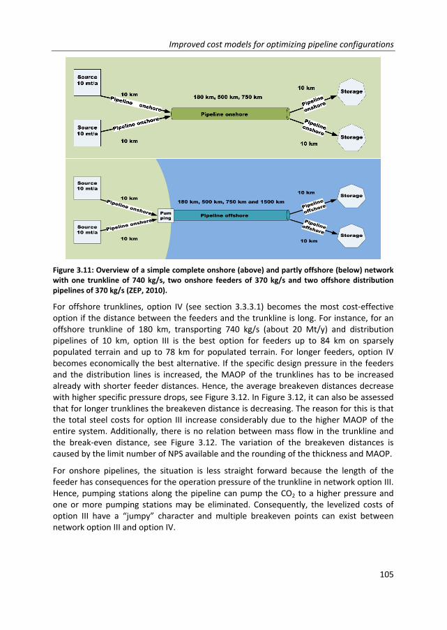
Improved cost models for optimizing pipeline configurations
105
Figure 3.11: Overview of a simple complete onshore (above) and partly offshore (below) network with one trunkline of 740 kg/s, two onshore feeders of 370 kg/s and two offshore distribution pipelines of 370 kg/s (ZEP, 2010).
For offshore trunklines, option IV (see section 3.3.3.1) becomes the most cost‐effective option if the distance between the feeders and the trunkline is long. For instance, for an offshore trunkline of 180 km, transporting 740 kg/s (about 20 Mt/y) and distribution pipelines of 10 km, option III is the best option for feeders up to 84 km on sparsely populated terrain and up to 78 km for populated terrain. For longer feeders, option IV becomes economically the best alternative. If the specific design pressure in the feeders and the distribution lines is increased, the MAOP of the trunklines has to be increased already with shorter feeder distances. Hence, the average breakeven distances decrease with higher specific pressure drops, see Figure 3.12. In Figure 3.12, it can also be assessed that for longer trunklines the breakeven distance is decreasing. The reason for this is that the total steel costs for option III increase considerably due to the higher MAOP of the entire system. Additionally, there is no relation between mass flow in the trunkline and the break‐even distance, see Figure 3.12. The variation of the breakeven distances is caused by the limit number of NPS available and the rounding of the thickness and MAOP.
For onshore pipelines, the situation is less straight forward because the length of the feeder has consequences for the operation pressure of the trunkline in network option III. Hence, pumping stations along the pipeline can pump the CO2 to a higher pressure and one or more pumping stations may be eliminated. Consequently, the levelized costs of option III have a “jumpy” character and multiple breakeven points can exist between network option III and option IV.

Chapter 3
106
No.
OD
trunkline
(m)
OD
feeders
(m)
LCb
(€/t)
OD
trunkline
(m)
OD
feeders
(m)
P_ inlet
(MPa)
Poutlet
(MPa)
cNpumps
Netw
ork
optiond
LCAlle
(€/t)
LCtranse
(€/t)
0.76
0.61
14
80
III
13.3
1.97
0.76
0.61
12
60
III
13.2
1.92
0.91
0.61
14
80
III
17.1
5.77
0.76
0.61
21
60
III
17.0
5.23
0.91
0.61
17
80
III
20.3
8.81
0.91
0.61
15
60
III
20.0
8.57
1.07
0.61
16
80
III
32.9
21.4
1.07
0.61
14
60
III
31.8
20.5
33
180
Onshore
2 x 1,330
10
0.81
0.51
1.5
0.76
0.61
98
4III
13.1
1.96
34
500
Onshore
2 x 1,330
10
0.81
0.51
0.76
0.61
10
86
III
15.8
4.64
35
750
Onshore
2 x 1,330
10
0.81
0.51
0.76
0.61
10
810
III
17.9
6.74
This modela
ZEP
Length
feeders &
distribution
lines (km)
Mass flow
(t/h)
Location
trunkline
Length
trunkline
(km)
II = Gaseous transport in
the feeders and liquid transport at the trunkline and distribution pipelines;
III = Liquid transport in
the entire netw
ork, w
here the streams flow im
mediately from the feeders into the trunkline without a pumping station;
IV = Liquid transport in
the entire netw
ork, having a pumping station installed just before at the inlet of the trunkline.
e)LCALLrefersto
thelevelizedcostsassociatedwithinitialcompression,pipelineandpumpingstations,whileLC
transreferto
thecostsassociatedwith
only pipeline and pumping stations.
2 x 1,330
2 x 1,330
2 x 1,330
2 x 1,330
a) Theonshore
pipelinecostsgivenin
theZEPrapportare
specificforflattopography,simplesoilconditionsandunobstructedROW.Therefore,the
resultsofthismodelforonshore
pipelinesare
basedonsparselypopulatedterrainandsteelgradesavailablein
theshortterm
.Furtherm
ore,inthe
ZEPreportitisassumedthattheyearlyoperationtimeis7500hours.Thisnumberisalsousedforcalculatingthecostsandconfigurationsin
this
table.
b) Thelevelizedcost
oftheZEPstudyincludesthepipelineitselfandinterm
ediate
pumpingstations.
Thecost
forcompressiontill11MPaand
dehydrationoftheCO2are
includedin
thecapture
costsandnotin
thetransportationcosts.
Thenumberofpumpingstationsincludedin
the
configuration is not mentioned.
c) In
thisstudy,thestandard
outletpressure
is8MPa.In
theZEPstudy,theoutletpressure
is8MPaforonshore
pipelinesand6MPaforoffshore
pipelines. Hence, the results of the model are calculated for 8 as well as for 6 MPa for the offshore cases.
d) A
s described in
the methodology:
I = Gaseous transport in
the feeders as well as in the trunkline and distribution pipelines;
5.3
3.7
0.51
8.2
16.3
31
750
Offshore
10
0.66
0.51
32
1,500
Offshore
10
0.76
0.51
3.4
6.0
29
180
Offshore
10
0.56
0.51
30
500
Offshore
10
0.66
Table 3.5: C
omparison of diameters and costs of an
onshore netw
ork from ZEP
and this m
odel.

Improved cost models for optimizing pipeline configurations
107
Figure 3.12: Breakeven feeder distance between option III (no pumping station before trunkline) and IV (pumping station before trunkline) for an offshore trunkline transporting liquid CO2 with two distribution lines of 10 km with an average (30 Pa/m for liquid CO2), high (+50%) or low (‐50%) design pressure drop. On the left, the distance of the trunkline is varied and the mass flow is kept constant at 740 kg/s (= 20 Mt/y with an operation time of 7,500 hours). On the right, the length of the trunkline is fixed at 180 km and the mass flows (with an operation time of 7,500 hours) is varied.
For networks with short trunklines and low mass flow rates, gaseous CO2 transport in whole the network (option I) can be the most cost‐effective. In Figure 3.13, the breakeven distance between gaseous transport in whole the network (option I) and liquid transport in part of or whole the network (option II, III or IV) can be seen for different trunkline lengths, various mass flows and three different design pressure drops. It is clear that the breakeven feeder distance is decreasing with increasing trunkline lengths until liquid CO2 transport in the trunkline is the most cost‐effective option regardless the feeder distance. Furthermore, the breakeven feeder distance is increasing with increasing mass flows.
Option II, where the CO2 is transported as a gas through the feeders and compressed to a liquid just before the trunkline, is in a few cases the most cost‐effective. For instance, option II gives the lowest levelized costs for a mass flow of 2 x 75 kg/s, a trunkline of 200 km, feeders and distribution lines of 10 km on sparsely populated terrain, namely 16.0 €/t compared to 19.9 €/t, 16.2 €/t and 16.4 €/t for option I, III and IV, respectively. The main reason for this is that the overall compression capacity required for this option (46 MW) is slightly lower than for complete liquid CO2 transport (50 MW), due to the lower pressure drop in the feeders. However, this is mainly the result of the assumption that the specific pressure drop is lower for gaseous than for liquid CO2 transport.
0
20
40
60
80
100
120
140
0 500 1000 1500
Break
even feeder distance (km
)
Length of trunkline (km)
Average ΔP High ΔP Low ΔP
0
20
40
60
80
100
120
140
0 200 400 600 800
Break
even feeder distance (km
)
Mass flow (kg/s)
Average ΔP High ΔP Low ΔP

Chapter 3
108
Figure 3.13: Breakeven feeder distance between gaseous transport in whole the network (option I) and liquid CO2 transport in part of or whole the network (option II, III or IV) with a trunkline and distribution lines of 10 km on sparsely populated terrain. On the left, the distance of the trunkline is varied for three different mass flows (100, 150 and 300 kg/s with an operation time of 7,500 hours). On the right, the length of the trunkline is fixed at 50 km and the mass flows (with an operation time of 7,500 hours) is varied for three different specific design pressure drops in the feeders and distribution lines.
Timing aspects 3.5.5
In the previous section, it was assumed that two sources are transporting CO2 from the same moment onwards. However, in reality it is likely that one source wants to transport from, for instance, 2020 onwards while the second source starts from 2025 or 2030. In Table 3.6, the configurations and levelized costs are calculated for several combinations of distances between the sources, distances of the trunkline and mass flows of two different sources. Several observations can be made:
‐ It appears more cost‐effective to combine the sources in a trunkline if the sink is further away from the sources (case 36‐37). Consequently, the sources can be further apart from each other.
‐ If the sources have unequal mass flows, it is often cost‐effective to construct a trunkline, if the source which come available first has the largest mass flow (case 38‐41).
‐ Two point‐to‐point‐pipelines of 100 km have in most cases slightly lower levelized costs than a trunkline of 100 km for two equally sized sources separated 10 km from each other coming available 10 years after each other (case 42‐45). Hence, the additional costs of over‐dimensioning a pipeline are almost similar to the costs of constructing a complete new point‐to‐pipeline in 2030 due to discounting. This effect will become stronger if the time difference between the availability of the sources is enlarged. For similar distances and mass flows, but now with a time difference of 5
0
20
40
60
80
100
120
0 25 50 75 100
Break
‐even feeder distance
Length of trunkline
Mass = 100 kg/s Mass = 150 kg/s Mass = 200 kg/s
0
20
40
60
80
100
120
0 50 100 150 200 250
Break‐even feed
er distance
Mass flow (kg/s)
Average ΔP High ΔP Low ΔP

Improved cost models for optimizing pipeline configurations
109
years, the trunkline configuration results in all cases (48‐51) in slightly lower levelized costs than the point‐to‐point pipeline configuration. The differences in LC between the trunkline and point‐to‐point pipeline configuration are however small, especially considering the uncertainties in the different cost models. Nevertheless, it can be concluded that a trunkline configuration becomes less cost‐effective with increasing time delays and two point‐to‐point pipelines are preferred after a time delay of about 5‐10 years.
‐ With a time difference of 5 years, the sources can be further apart from each other and still be cost‐effectively combined in a trunkline (compare 46‐47 with 52‐53).
If the trunkline option is the most cost‐effective approach and the second source is not coming available, then the levelized costs will increase to above the level of the point‐to‐point pipeline approach. For instance, for a trunkline length of 100 km, feeders of 10 km on sparsely populated terrain and two mass flows of 100 kg/s coming available 5 years after each other, the levelized costs of combining the two sources would be 12.3 €/t (1.7 €/t excluding compression) but if the second source would not become available they will increase to 13.3 €/t (2.6 €/t excluding compression) while the levelized costs for a separate point‐to‐point pipeline would be 12.5 €/t (2.0 €/t excluding compression).
Implications of the system boundaries 3.5.6
In this study, gaseous and liquid CO2 transport are compared and in several cases gaseous transport resulted in lower levelized costs than liquid CO2 transport. However, the system boundaries have been placed before the injection well. If CO2 storage requirements are taken into account the preference between gaseous and liquid CO2 transport could change. To analyze this, two different cases are explored. Firstly, a case with a required injection pressure of 8 MPa, which represents injection in an aquifer. Secondly, a case representing injection in a depleted gas field, where the required injection pressure increase linearly in three years from 1.5 MPa to 8 MPa and then remains on 8 MPa for the rest of the lifetime.30 For this analysis, it is assumed that a stand‐alone compressor is as expensive as the initial compressor near the capture plant.
For the first case, the gaseous CO2 has to be compressed at the storage location from the original pressure of 1.5 MPa to the required injection pressure of 8 MPa. This results in costs of 5.1 €/t for 100 kg/s CO2. These additional costs are enough to cancel out the cost advantage of gaseous compared to liquid CO2 transport, which was 0.9 €/t for 100 km and 2.3 €/t for a 50 km pipeline over sparsely populated land. Similar results are found for other mass flows and pipeline length. Thus, if the CO2 has to be injected with a pressure of 8 MPa, it is more cost‐effective to transport CO2 as a liquid than as a gas.
30 In practice, the required injection pressure will further increase. However, this will be similar for the gaseous
and liquid CO2 case and does not change the preference. Therefore, it is not included.

Chapter 3
110
Table 3.6: Netw
ork optimization for tw
o sources which become available in different time frames, w
here the first source becomes
available in
2020.
Length
trunk
Length
feeder
(km
) (km
)I
IITr.
PtP I
PtP II
Tr.PtP IPtP II
Tr.
PtP IPtP II
LCALL
PtP
LCtrans
PtP
LCALL
Trunk
LCtrans
Trunk
36200
10200
2030
S. Pop.
150
150
1211
111
11
0.51
0.41
0.41
14.6
3.45
14.5
3.36
37500
10500
2030
S. Pop.
150
150
1110
106
76
0.51
0.41
0.41
20.1
9.00
19.6
8.52
38200
10200
2030
S. Pop.
200
100
1212
111
22
0.51
0.41
0.32
14.1
3.16
13.9
2.93
39200
10200
2030
S. Pop.
100
200
1211
121
22
0.51
0.32
0.41
14.7
3.68
15.0
3.95
40200
10200
2030
S. Pop.
50100
1113
111
32
0.41
0.22
0.32
16.9
5.53
17.3
5.95
41200
10200
2030
S. Pop.
100
5011
1114
12
20.41
0.32
0.22
15.8
4.65
15.5
4.39
42100
10100
2030
S. Pop.
5050
1318
170
00
0.32
0.22
0.22
14.7
2.84
14.5
2.97
43100
10100
2030
S. Pop.
100
100
1413
120
01
0.41
0.32
0.32
13.1
1.98
13.0
1.92
44100
10100
2030
S. Pop.
200
200
1014
131
01
0.61
0.41
0.41
12.3
1.27
12.4
1.49
45100
10100
2030
S. Pop.
500
500
910
121
10
0.91
0.61
0.61
11.6
0.84
11.7
0.98
46200
25200
2030
S. Pop.
100
100
1211
112
22
0.41
0.32
0.32
15.4
4.3
15.2
4.13
47200
50200
2030
S. Pop.
100
100
1211
112
22
0.41
0.32
0.32
15.4
4.3
15.4
4.31
48100
10100
2025
S. Pop.
5050
1318
180
00
0.32
0.22
0.22
14.7
2.85
14.2
2.59
49100
10100
2025
S. Pop.
100
100
1413
130
00
0.41
0.32
0.32
13.1
1.99
12.8
1.68
50100
10100
2025
S. Pop.
200
200
1014
141
00
0.61
0.41
0.41
12.3
1.28
12.2
1.35
51100
10100
2025
S. Pop.
500
500
910
101
11
0.91
0.61
0.61
11.6
0.87
11.5
0.87
52200
50200
2025
S. Pop.
100
100
1211
112
22
0.41
0.32
0.32
15.4
4.33
15.2
4.05
53200
75200
2025
S. Pop.
100
100
1211
112
22
0.41
0.32
0.32
15.4
4.33
15.5
4.33
b)
S. Pop., popu. and offsh. refers to sparsely populated, populated terrain and offshore pipelines, respectively.
c) TheabbreviationsTr,PtP
I,andPtP
IIreferto
trunkline,
point‐to‐pointpipelinefrom
sourceI,andpoint‐to‐pointpipelinefrom
sourceIIto
thesink,
d)
LCALLrefers
tothelevelizedcostsassociatedwithinitialcompression,pipelineandpumpingstations,whileLC
transreferto
thecostsassociatedwithonly
pipeline and pumping stations. The network approach
(point‐to‐point pipelines or trunkline) which result in the lowest LC
ALL, is italic and bold.
Npumpsc
Diameterc
Levelized costs (€/t CO2)c,d
Mass flow
(kg/s)
a)
In 2025, the same steel grades are available as in the short term.
No.
Distance
source II ‐
sink (km)
Source II
a
availa‐
bility
Terrainb
Inlet pressure
c

Improved cost models for optimizing pipeline configurations
111
For the second case, a compressor has to be installed in the second year which is able to compress the gaseous flow to 3.7 MPa in the second year, to 5.8 MPa in the third year and to 8 MPa from year four onwards. For a mass flow of 100 kg/s, a compressor of 11 MWe is needed. This increases the levelized costs with 3.5 €/t and results in total levelized costs of 13.2 €/t and 15.6 €/t for 50 and 100 km pipeline on sparsely populated terrain. Note that in the first few years, liquid CO2 has to be decompressed so that it can injected in the depleted gas field. However, this will lead to a large drop in temperature and injection of cold CO2 can lead to hydrate formation in the well and to thermal cracking of the surrounding rocks in the well formation. Therefore, an electric heater is required to increase the injection temperature to 0°C, which is estimated to be high enough to avoid hydrate formation and thermal cracking (E.ON, 2011d). A heater of 20 MW is installed and used for two years.31 With estimated heater costs of 1 M€/MW (E.ON, 2011cd)32 and O&M costs of 4% of the capital costs, the heater increases the levelized costs with 1.6 €/t for a mass flow of 100 kg/s. Combining these costs with the initial compression and transportation costs, leads to levelized costs for liquid CO2 transport of 13.4 €/t and 14.1 €/t for 100 kg/s over 50 and 100 km sparsely populated terrain, respectively. If these costs are compared with the levelized costs for gaseous CO2 transport, the costs for liquid CO2 transport are lower for the 100 km but higher for 50 km case.
To conclude, for storage reservoirs with a high reservoir pressure, liquid CO2 transport appear the best option. For depleted gas fields with a low reservoir pressure, the cost effectiveness of liquid or gaseous CO2 transport depends on the source‐sink distance, mass flow and on how quickly the required injection pressure increase over time. Gaseous CO2 transport seems to be especially interesting for small CO2 mass flows on a close distance from a depleted gas field with a low reservoir pressure.
Sensitivity analysis 3.5.7
A sensitivity analysis is conducted to assess the robustness of the optimal configuration and the impact on the levelized costs for point‐to‐point pipelines. Four of the main economic input parameters are varied, namely the interest rate, electricity, steel and labor costs (Table 3.1). The sensitivity analysis is conducted for different mass flows,
31 Isobaric heating and adiabatically expansion is assumed by calculating the energy required for heating up the
CO2. In the first year, the CO2 is injected with a pressure of 1.5 MPa and temperature of 0°C and delivered at 8.0 MPa and temperature of 15°C. To ensure similar enthalpy levels before and after expansion, the CO2 has to be first heated up to 72°C. Because the specific heat under isobaric conditions varies quite a lot over this temperature range (Span and Wagner, 1996), a weighted average of the heat capacity is used. Subsequently, the required heater capacity is calculated by assuming a heater efficiency of 100%, (m x Cp x ΔT / η = 100 kg/s x 3.44 kg/kJ/K x (72‐15) / 100% = ) 19.6 MW. 32 In literature, costs for large electric heaters are not available, as far as the authors know. In the FEED study of
E.ON, 4 heaters of 1.05 MW are included (E.ON, 2011d). The costs for this are probably included in the category ‘well interface’, together with the choke valve, safety valve and metering equipment. In total, this category costs 4.66 M€2010 (E.ON, 2011c). Based on this information the costs of the heater are estimated at 1 M€/MW.

Chapter 3
112
lengths, time frames and terrain types. In total about 50 cases are analyzed and 20 of them focus on pipelines transporting liquid CO2 over sparsely populated terrain in the short term. The results of one case are given in Table 3.7, but results of all runs are reported in Annex G.
The average consequences of a 50% increase in interest rate, steel price, electricity or labor costs on the levelized costs including and excluding compression are shown in Figure 3.14. The results indicate that the total levelized costs are mostly influenced by the electricity costs due to the high compression energy. If the compression costs are excluded, the interest rate and labor have the largest impact followed by steel and electricity costs. Similar trends can be seen when the parameters are all increased by 100%.
However, the labor costs are more uncertain than the other three variables. Hence, a 100% increase in the labor costs is assumed to be as likely as a 50% increase in the interest rate, electricity and steel costs. If these realistic ranges are taken into account, the levelized costs including compression are still mostly influenced by the electricity costs, see Figure 3.14. However, the levelized costs without compression are now most influenced by the uncertainty in labor costs.
Besides influencing the levelized costs, varying a parameter e.g. with 50% or 100% can also lead to a different optimal pipeline configuration (see Table 3.7 and Annex G). Overall, changings on the steel price has the largest impact on the optimal inlet pressure. For instance, at a lower steel price, it is more cost‐effective to invest in a pipeline with a thicker wall and install less pumping stations along the route.
Table 3.7: Sensitivity results of one case for transporting 500 kg/s CO2 over 100 km sparsely populated terrain. A complete overview of all cases can be found in Annex F.
OD (m)
Pinlet
(MPa) Npumps LCALL
a
(€/t CO2)
LCtrans
(€/t CO2) Pressure drop (Pa/m)
Lpump (km)
Base case 0.61 10 1 11.6 0.84 38 52 Electricity costs ‐50% 0.61 10 1 7.02 0.81 38 52
+50% 0.76 9 1 16.2 0.95 12 84 Steel costs ‐50% 0.61 12 0 11.5 0.64 40 101
+50% 0.61 10 1 11.7 0.94 38 52 Labor costs ‐50% 0.76 9 1 11.4 0.66 12 84
+50% 0.61 10 1 11.9 1.08 38 52 +100% 0.61 10 1 12.1 1.31 38 52
Interest rate ‐50% 0.76 9 1 10.9 0.57 12 84 +50% 0.61 10 1 12.4 1.16 38 52
a) LCALL refers to the levelized costs associated with initial compression, pipeline and pumping stations, while LCtrans refer to the costs associated with only pipeline and pumping stations.

Improved cost models for optimizing pipeline configurations
113
Figure 3.14: The average consequences of an increase in interest rate, steel, electricity, and labor costs on the levelized costs, for CO2 transport on flat sparsely populated terrain, including (left) and excluding compression costs (right).
In contrast, it is often cost‐effective to install a larger diameter to limit the specific pressure drop if the interest rate or labor costs decrease or the electricity costs increase. The initial higher investment costs are compensated by the lower energy consumption during the lifetime. In most cases, the optimal configuration does not change with a 50% increase in the interest rate or labor costs. However, with a 100% increase in the labor costs or with a 50% reduction in the electricity costs, the selection of a smaller diameter is cost‐effective in several cases.
Overall, offshore cases appear less sensitive to changes in the interest rate, electricity, steel and labor costs than onshore cases, because the option to add or eliminate pumping stations is not available. Hence, the cost minimization is only driven by the NPS available. This argument is also valid for gaseous CO2 transport.
Additionally, it has also been examined whether a different interest rate could affect the cost‐effectiveness of a trunkline versus point‐to‐point pipelines when two sources come available in different time frames. For this, 35 cases were run with a time difference of 5 or 10 years between the availability of the first and second CO2 source (see Annex G for the results per case). If the interest rate is increased to 15%, the cost‐effectiveness of the trunkline decreases compared to the point‐to‐point pipeline configuration. The reason for this is the strong discount effect of, in particular, the second point‐to‐point pipeline. Consequently, even with a time difference of only five years between two equally sized sources 10 km apart from each other, several cases prefer two point‐to point pipelines to a trunkline. The opposite is also true, a lower interest rate has a positive effect on the trunkline configuration. With respect to configuration changes, similar trends were observed as described above for the trunkline as well as for the point‐to‐point pipeline configurations.
0%
10%
20%
30%
40%Steel
Electricity
Labor
Interest rate
Realistic ranges
50% increase for all variables
0%
20%
40%
60%Steel
Electricity
Labor
Interest rate
Realistic ranges
50% increase for all variables

Chapter 3
114
Conclusion 3.6
This study had two main aims. Firstly, to develop a new cost model for CO2 pipeline transport related to the physical properties of CO2, and secondly to develop a cost minimization model to determine the optimal configuration for point‐to‐point pipelines as well as for simple networks.
The new pipeline cost model explicitly takes into account differences in operation pressure and materials. The results indicate that low steel grades, such as X42 and X52, lead to the lowest capital costs for pipelines transporting gaseous CO2, while higher steel grades lead to the lowest capital costs for onshore pipelines transporting liquid CO2. For instance, for an onshore pipeline with a diameter of 0.61 m and a MAOP of 15MPa, using X120 instead of X80 results reduces the capital costs with 7‐8%. As a consequence, the highest available steel grades are selected for onshore pipelines transporting liquid CO2, namely X80 in the short term, X100 in the medium term and X120 in the long term. Offshore pipelines remain mainly based on lower steel grades because for these pipelines the thickness should be minimal 2.5% of the outer diameter. Also pipelines transporting gaseous CO2 do not benefit from higher steel grades, due to the low operation pressure.
A cost minimization model was developed which include initial compression, pipeline, steel grades and pumping stations to determine the most cost‐effective configuration for CO2 pipeline transport. Slightly different methodologies were developed for point‐to‐point pipelines and simple networks over one or multiple kinds of terrain (sparsely populated, populated and offshore). Figure 3.15 summarizes the key conclusions for each type of pipeline.
From a chain perspective, gaseous CO2 transport can have lower levelized costs than liquid CO2 transport point‐to‐point pipelines as well as for simple networks. Gaseous CO2 transport seems to be especially interesting for small CO2 mass flows on a close distance from a depleted gas field with a low reservoir pressure. The reason for this is that the lower initial compression costs compensate the higher pipeline costs. However, for storage reservoirs with a high reservoir pressure (like aquifers), liquid CO2 transport is more cost‐effective than gaseous CO2 transport.
For offshore pipelines, the optimal inlet pressure is directly influenced by the length, because in this case pumping stations are not an option. The inlet pressure can become up to about 25 MPa. For even longer pipelines, a larger diameter is selected to limit the specific pressure drop. For instance, for a pipeline transporting 300 kg/s liquid CO2 (about 9 Mt/y) the optimal inlet pressure is 12 MPa for 100 km and 22 MPa for 340 km, leading to an average pressure drop of about 45 Pa/m. If the distance increases to 350 km, a larger diameter is selected (namely 0.61 m instead of 0.41 m) to limit the inlet pressure (to 14 MPa) and the specific pressure drop (to 14 Pa/m). This results in levelized costs (excluding compression) of 1.4 and 4.8 €/t for transporting 300 kg/s CO2 over 100 and 350 km, respectively. For larger mass flow rates, the levelized costs are decreasing.

Improved cost models for optimizing pipeline configurations
115
Simple network Point‐to‐point pipelines
Single
terrain
‐ Gaseous CO2 transport can result in lower levelized costs than liquid CO2 transport, if the CO2 is stored in reservoirs with a low pressure. Gaseous CO2 transport is especially interesting for small CO2 mass flow and short distances.
‐ Liquid onshore CO2 transport: Pinlet = 9‐13 MPa; ΔP = 15‐45 Pa/m
‐ Liquid offshore CO2 transport: ΔP = 10‐50 Pa/m,
‐ Gaseous transport: ΔP = 5‐20 Pa/m
‐ All four network options result for some combination of mass flow and length in the lowest levelized costs.
‐ However, transporting gaseous CO2 and compress it to a liquid just before the trunkline is only interesting in a few cases and this is mainly due to the assumptions made about design pressure drop.
‐ The maximum distance of feeders ‐ without a pumping
stations before the offshore trunk‐line increases with decreasing trunkline lengths. For instance, the max. distance is 75 km for a 100 km and 40 km for a 1,000 km long offshore trunkline.
Break‐even distances are independent of mass flow, but variation is present due to the limited NPS available.
‐ Gaseous CO2 transport in whole the network can be cost‐effective for short networks and limited mass flows.
‐ The levelized costs increase with 8% to 18% for a 100 km pipeline when the terrain change from sparsely populated to populated terrain.
‐ For longer pipelines the cost increase is slightly less due to similar costs for pumping stations in different types of terrain.
‐ The ΔP is slightly higher on populated than on sparsely populated terrain.
Timing aspectsTwo point‐to‐point pipelines are cost‐attractive compared to a trunkline: ‐ With Δt = 5‐10 years ‐ If the source with the smallest mass flow come available first.
‐ When the distance between the source and the sink is small.
Multip
le te
rrain
Figure 3.15: Main conclusions of the cost minimization model, divided in point‐to‐point pipelines and simple networks over a single or multiple terrain types.
The assessment also indicates that the optimal diameter, and hence the specific pressure drop, is mainly influenced by a decrease in the labor costs and interest rate or a change in electricity costs. Changes in the steel costs affect primarily the optimal inlet pressure of the pipeline, and consequently the distance between pumping stations. Furthermore, the sensitivity analysis showed that changes in the electricity costs have the largest influence on the total levelized costs due to the high compression costs. However, if the compression costs are excluded from the levelized costs, the labor costs and interest rate have the largest impact followed by the steel and electricity costs.
There are still a number of points in which way the cost minimization model can be improved further:

Chapter 3
116
‐ A network design will not only be based on economic optimums but will also depend on legislation, operational preference, risk and safety aspects. Furthermore, reliability considerations will be important.
‐ The current version of the model was not linked to topographical maps and different types of terrain (offshore, sparsely populated and populated) serve as a manual input.
‐ Impurities were not taken into account and these would influence the phase envelope and the physical properties of the CO2. Hence, it will affect the capacity, the minimum pressure and the material requirements of the pipeline.
References 3.7‐ AG Der Dillinger Hüttenwerke, GTS industries SA., 2012. Heavy plate steel price list.
Last accessed in 2012. ‐ Apeland, S., Belfroid, S., Santen, S., Hustad, C.W., Tettero, M. et al., 2011a. Towards a
transport infrastructure for large‐scale CCS in Europe. Kårstø CO2 pipeline project: Extension to a European case. CO2 Europipe D4.3.2, 1‐84.
‐ Apeland, S., Belfroid, S., Santen, S., Hustad, C.W., Tettero, M., Klein, K., 2011b. Towards a transport infrastructure for large‐scale CCS in Europe. Kårstø offshore CO2 pipeline design. CO2 Europipe D4.3.1, 1‐95.
‐ Austell, M., Van der Brugt, A., Neele, F., Tetteroo, M., Ros, M. et al., 2011. Towards a transport infrastructure for large‐scale CCS in Europe. Development of large scale CCS in The North Sea via Rotterdam as CO2 hub. CO2 Europipe D4.1.1, 1‐102.
‐ Brauer, H., Knauf, G., Hillenbrand, H.G., 2004. Crack arrestors. 4th International conference on pipeline technology.
‐ Bureau, G., Roussanaly, S., Husebye, J., 2011. Cocate. Large‐scale CCS transportation infrastructure in Europe. Economic assessment of CO2 export systems and comparison of implementation strategies. COCATE D4.1.2, 1‐181.
‐ Cayrade, P., 2004. Investment in gas pipelines and liquefied natural gas infrastructure. What is the impact on the security of supply? INDES Working paper no.3, 1‐12.
‐ Chandel, M.K., Pratson, L.F., Williams, E., 2010. Potential economies of scale in CO2 transport through use of a trunk pipeline. Energy Conversion and Management 51, 2825‐34.
‐ Code of Federal Regulation, 2010. Title 49: Transportation. Last accessed in 2013. Retrieved from: http://cfr.vlex.com/source/code‐federal‐regulations‐transportation‐1098/toc/02.01.
‐ ChemicaLogic, 1999. Carbon dioxide phase diagram. Last accessed in 2013. Retrieved from: www.chemicalogic.com/Pages/DownloadPhaseDiagrams.aspx.
‐ Cole, I.S., Corrigan, P., Sim, S., Birbilis, N., 2011. Review. Corrosion of pipelines used for CO2 transport in CCS: Is it a real problem? International Journal of Greenhouse Gas Control 5, 749‐56.
‐ CRU, 2012. CRU steel price index. Last accessed in 2012. Retrieved from:
www.cruonline.crugroup.com. ‐ Dahowski, R.T., Dooley, J.J., Davidson, C.L., Bachu, S., Gupta, N., 2004. A CO2 storage
supply curve for North America. PNWD‐3471, 1‐92. ‐ Damen, K., van Troost, M., Faaij, A., Turkenburg, W., 2007. A comparison of electricity

Improved cost models for optimizing pipeline configurations
117
and hydrogen production systems with CO2 capture and storage‐Part B: Chain analysis of promising CCS options. Progress in Energy and Combustion Science 33, 576‐605.
‐ DNV, 2010. Recommended practice. Design and operation of CO2 pipelines. DNV‐RP‐J202, 1‐42.
‐ DNV, 2012. Offshore standard. Submarine pipeline systems. DNV‐OS‐F101, 1‐215. ‐ Downie, M., 2011. CO2 transport in CCS. UKCCS Winter School, School of Marine
Technology. University of Newcastle. ‐ E.ON, 2011a. Kingsnorth Carbon Dioxide Capture and Storage Demonstration Project.
Key Knowledge Reference Book. 1‐66. ‐ E.ON, 2011b. Kingsnorth Carbon Capture and Storage Project. Onshore Pipeline
Project Data. Rev. 4. KCP‐GNS‐PLD‐DPR‐0005. 1‐14. ‐ E.ON. 2011c. Kingsnorth Carbon Capture & Storage Project. Post‐FEED Project Cost
Estimates. Rev. 1. KCP‐EUK‐FIN‐LIS‐0002. 1‐2. ‐ E.ON. 2011d. Kingsnorth Carbon Capture & Storage Project. Offshore Heater Option
Evaluation & Concept Design Report (Gaseous Phase). Rev. 2. KCP‐GNS‐PCD‐DRP‐0002. 1‐6.
‐ EBN and Gasunie, 2010. CO2 transport‐ en opslagstrategie. EBN / Gasunie advies, 1‐95. ‐ ElementEnergy, 2010. CO2 pipeline infrastructure: An analysis of global challenges and
opportunities. IEA GHG 1‐134. ‐ EU GeoCapacity, 2008. Assessing European capacity for geological storage of carbon
dioxide. Publishable final activity report. SES6‐518318, 1‐37. ‐ European Commission, 2011. Communication from the commission to the European
parliament, the council, the European economic and social committee and the committee of the regions. A roadmap for moving to a competitive low carbon economy in 2050. COM(2011) 112 final, 1‐16.
‐ Felber, S., Loibnegger, F., 2009. The pipeline steels X100 and X120. XI‐929‐09, 1‐24. ‐ Fimbres Weihs, G.A., Wiley, G.A., 2012. Steady‐state design of CO2 pipeline networks
for minimal cost per tonne of CO2 avoided. International Journal of Greenhouse Gas Control 8, 150‐168.
‐ Gao, L., Fang, M., Li, H., Hetland, J., 2011. Cost analysis of CO2 transportation: Case study in China. Energy Procedia 4, 5974‐81.
‐ GCCSI, 2012. The global status of CCS 2012. 1‐218. ‐ Gräf, M.K., Hillenbrand, H.G., Heckmann, C.J., Niederhoff, K.A., 2003. High‐strength
large‐diameter pipe for long‐distance high pressure gas pipelines. Proceedings of the International Offshore and Polar Engineering Conference, 2347‐54.
‐ Hillenbrand, H.G., Graef, M.K., Gross‐Weege, J., Knauf, G., Marewski, U., 2001. Development of line pipe for deep water applications. Europipe, 1‐9.
‐ Hillenbrand, H.G., Liessem, A., Kalwa, C., Erdelen‐Peppler, M., Stallybrass, C., 2008. Technological solutions for high strength gas pipeline. Europipe technical paper, 1‐16.
‐ IEA, 2009. Technology Roadmap. Carbon capture and storage. IEA publications, Paris, France.
‐ IEA, 2010. World energy outlook 2010. Organisation for Economic Co‐operation and Development (OECD) / International Energy Agency (IEA).
‐ IEA GHG, 2002. Pipeline transmission of CO2 and energy. Transmission study report.

Chapter 3
118
PH4/6, 1‐140. ‐ IEA GHG, 2007. Distributed collection of CO2. 2007/12, 1‐109. ‐ IEA GHG, 2008. Co‐production of hydrogen and electricity by coal gasification with CO2
capture ‐ updated economic analysis. 2008/9, 1‐528. ‐ IHS, 2013. IHS indexes. IHS/CERA upstream capital cost index (UCCI). Last accessed in
2013. Retrieved from: http://www.ihs.com/info/cera/ihsindexes/index.aspx. ‐ Interliance LLC for California Energy Commission, 2002. Gulf coast to California
pipeline feasibility study. Consultant report P699‐02‐010DCR, 1‐32. ‐ Knoope, M.M.J., Ramírez, A., Faaij, A.P.C., 2013. A state‐of‐the‐art review of techno‐
economic models predicting the costs of CO2 pipeline transport. International Journal of Greenhouse Gas Control 16, 241‐70.
‐ Kreutz, T.G., Larson, E.D., Liu, G., Williams, R.H., 2008. Fischer‐Tropsch fuels from coal and biomass. Princeton Environmental Institute Prepared for 25th Annual International Pittsburgh Coal Conference. 29 September – 2 October, 2008 Pittsburgh, Pennsylvania, USA, 1‐86.
‐ Kreutz, T.G., Williams, R., Consonni, S., Chiesa, P., 2005. Co‐production of hydrogen, electricity and CO2 from coal with commercially ready technology. Part B: Economic analysis. International Journal of Hydrogen Energy 30, 769‐784.
‐ Kuramochi, T., Ramírez, A., Turkenburg, W., Faaij, A., 2012. Comparative assessment of CO2 capture technologies for carbon‐intensive industrial processes. Progress in Energy and Combustion Science 38, 87‐112.
‐ Mallon, W., Guijt, W., 2012. Personal communication with W. Mallon (of DNV KEMA) and W. Guijt (of Shell) about costs and modeling of CO2 pipeline transport.
‐ McCoy, S. T., & Rubin, E. S. (2008). An engineering‐economic model for pipeline transport of CO2 with application to carbon capture and storage. International Journal of Greenhouse Gas Control, 2, 219‐229.
‐ Meerman, J.C., Ramírez, A., Turkenburg, W.C., Faaij, A.P.C., 2012. Performance of Flexible Multi‐fuel Integrated Gasification Poly‐Generation Facilities with CCS. Part B: An Economic Evaluation. International Journal of Greenhouse Gas Control 16, 6083‐102.
‐ Middleton, R.S., Bielicki, J.M., 2009. A scalable infrastructure model for carbon capture and storage: SimCCS. Energy Policy 37, 1052‐60.
‐ Middleton, R.S., Kuby, M.J., Wei, R., Keating, G.N., Pawar, R.J., 2012. A dynamic model for optimally phasing in CO2 capture and storage infrastructure. Environmental Modelling and Software 37, 193‐205.
‐ Mohitpour, M., Golshan, H., Murray, A., 2003. Pipeline design & construction. A practical approach. Second edition. ASME press, United States.
‐ Mohitpour, M., Seevam, P., Botros, K.K., Rothwell, B., Ennis, C., 2012. Pipeline transportation of carbon dioxide containing impurities. 1st edition. ASME Press, New York, USA.
‐ Moomaw, W., Yamba, F., Kamimoto, M., Maurice, L., Nyboer, J. et al., 2011. IPCC Special Report on Renewable Energy Sources and ClimateChange Mitigation. Cambridge University Press, Cambridge, United Kingdom and New York, USA.
‐ Morbee, J., Serpa, J., Tzimas, E., 2012. Optimised deployment of a European CO2

Improved cost models for optimizing pipeline configurations
119
transport network. International Journal of Greenhouse Gas Control 7, 48‐61. ‐ NIST, 2012. National Institute of Standards and Technology (NIST) standard reference
data. Thermophysical properties of fluid systems. Last accessed in 2012. Retrieved from: http://webbook.nist.gov/chemistry/fluid/.
‐ Nord Stream, 2012. Fact sheet Nord Stream by numbers. Last accessed in 2012. ‐ NORSOK, 2006. NORSOK standard. Process design. Edition 5 P‐001, 1‐22. ‐ OANDA, 2011. Historical exchange rates. Last accessed in 2011. Retrieved from:
http://www.oanda.com/. ‐ Piessens, K., Laenen, B., Nijs, W., Mathieu, P., Baele, J.M. et al., 2008. Policy Support
System for Carbon Capture and Storage. SD/CP/04A, 1‐269. ‐ Pipeline & Gas Journal, 2009. New low‐hydrogen stick electrode helps pipeline
contractor. Pipeline & Gas Journal 236. ‐ Preston, 2013. Preson pipe & tube report. United States & Canada. Preston Publishing
Company 31, 1‐69. ‐ Read, A., 2012. Case 1: ROAD project, Rotterdam. System integration challenges. CCS
system integration workshop; Calgary, Canada. ‐ Rui, Z., Metz, P.A., Chen, G., Zhou, X., Wang, X., 2012. Regressions allow development
of compressor cost estimation models. Oil and Gas Journal 101, 110‐115. ‐ ScottishPower CCS Consortium, 2011. UK Carbon Capture and Storage Demonstration
Competition. FEED Close Out Report. SP‐SP 6.0 ‐ RT015, 1‐65. ‐ Skovholt, O., 1993. CO2 transportation system. Energy Conversion and Management
34, 1095‐1103. ‐ Smith, C.E., 2006. US gas carriers' 2005 net incomes climb; construction costs
plummet. Oil and Gas Journal 104, 46‐63. ‐ Smith, C.E., 2010. Natural gas pipelines continue growth despite lower earnings; oil
profits grow. Oil and Gas Journal 108, 102‐118. ‐ Smith, C.E., True, W.R., Stell, J., 2005. US gas carriers see 2004 net jump; construction
plans rebound. Oil and Gas Journal 103, 50‐54. ‐ Smith, C.E., 2008. Natural gas pipeline profits surge; oil flat. Oil and Gas Journal 106,
50‐64. ‐ Smith, C.E., 2009. Special report: Pipeline profits, capacity expansion plans grow
despite increased costs. Oil and Gas Journal 107, 60‐72. ‐ Smith, C.E., 2012. Oil pipeline operators' 2011 profits soar to record. Oil and Gas
Journal 110, 112‐31. ‐ Smith, C.E., 2011. Special report: Pipeline construction plans continue slide despite
growth in natural gas. Oil and Gas Journal 109, 110‐121. ‐ Smith, C.E., 2007. Special report: US oil carriers' 2006 net incomes rebound; labor
increases push up construction costs. Oil and Gas Journal 105, 44‐58. ‐ Span, R., Wagner, W., 1996. A new equation of state for CO2 covering the fluid region
from the triple point to 1100 K at pressures up to 800 MPa. Journal of physical and chemical reference data 25, 1509‐1596.
‐ Spinelli, C.M., Demofonti, G., Fonzo, A., Lucci, A., Ferino, J., Di Biagio, M., Flaxa, V., Zimmermann, S., Kalwa, C., Knoop, F.M., 2011. Full scale investigation on strain capacity of high grade large diameter pipes. 18th Joint technical meeting on pipeline

Chapter 3
120
research, San Fransisco, USA, pp. 1‐16. ‐ Svensson, R., Odenberger, M., Johnsson, F., Strömberg, L., 2004. Transportation
systems for CO2 ‐ Application to carbon capture and storage. Energy Conversion and Management 45, 2343‐53.
‐ True, W.R., 2002. Special report. Pipeline economics: Fed data show solid 2001 for US pipeline companies, more gas capacity planned. Oil and Gas Journal 100, 52‐60.
‐ True, W.R., 2003. Special report: Pipeline economics. Oil and Gas Journal 101, 60‐90. ‐ True, W.R., Stell, J., 2004. US construction plans slide; pipeline companies experience
flat 2003, continue mergers. Oil and Gas Journal 102, 52‐70. ‐ Van den Broek, M., Brederode, E., Ramírez, A., Kramers, L., van der Kuip, M. et al.,
2010. Designing a cost‐effective CO2 storage infrastructure using a GIS based linear optimization energy model. Environmental Modelling and Software 25, 1754‐68.
‐ Van Ginkel, M., Speets, R., Holleman, E., Thonon, I., 2011. Milieueffectrapport CCS Maasvlakte (ROAD‐project). Royal Haskoning for ROAD. 9V7319.20, 1‐168.
‐ Van Osch, M., Smeulders, J., Veltin, J., 2010. Inventory and quantitative characterization of technologies available for each part of the CO2 infrastructure system. CATO‐2 Deliverable WP 2.1‐D03, 1‐42.
‐ Vattenfall, 2011. CCS demonstration project Jänschwalde. CO2 transport pipeline. FEED study. Non‐ confidential study co‐financed by the EU rev. 1. No. P10111.2011, 1‐142.
‐ Wildenborg, T., Holloway, S., Hendriks, C., Kreft, E., Lokhorst, A. et al., 2004. Cost curves for CO2 storage. Part 2: European sector. NITG 04‐238‐B1208, 1‐162.
‐ Woods, D.R., 2007. Rules of thumb in engineering practice. Wiley‐VCH Verlag GmbH & Co. KGaA, Weinheim, Germany.
‐ Yorkshire Forward, 2008. A carbon capture and storage network for Yorkshire and Humber. An introduction to understanding the transportation of CO2 from Yorkshire and Humber emitters into offshore storage sites. 05_08 100203, 1‐60.
‐ ZEP, 2010. CO2 transport costs. 1‐52. ‐ ZEP, 2011. The costs of CO2 Capture. Post‐demonstration CCS in the EU. 1‐81. ‐ Zhang, D., Wang, Z., Sun, J., Zhang, L., Li, Z., 2012. Economic evaluation of CO2 pipeline
transport in China. Energy Conversion and Management 55, 127‐35. ‐ Zhang, Z.X., Wang, G.X., Massarotto, P., Rudolph, V., 2006. Optimization of pipeline
transport for CO2 sequestration. Energy Conversion and Management 47, 702‐15.

121
Chapter 4: The influence of risk mitigation measures on the risks, costs and routing of CO2 pipelines
1
Abstract: The aim of this study was to analyze whether, and if so, in what way risks would influence the design, costs and routing of CO2 pipelines. This article assesses locational and societal risks of CO2 pipeline transport and analyses whether rerouting or implementing additional risk mitigation measures is the most cost‐effective option. The models EFFECTS and RISKCURVES are used to estimate the dispersion and risk, respectively. The pipeline routes are optimized by using the least cost path function in ArcGIS.
This article evaluates three case studies in the Netherlands. The results show that pipelines transporting dense phase CO2 (8‐17 MPa) with a minimal amount of risk mitigation measures already meet the 10‐6 locational risk required in the Netherlands. 10‐6 locational risks of 135 m are calculated for intermediate pumping stations, handling 450 kg CO2/s (about 14 Mt CO2/y). In all the cases, pumping stations could be located along the pipeline route without any problem.
For the cases studied transporting gaseous CO2 (1.5‐3 MPa) leads to larger 10‐6 locational risk distances than transporting dense phase CO2. This is caused by the large momentum behind a dense phase CO2 release, leading to smaller but higher jet and to a higher mixing rate with the surrounding air than for a gaseous CO2 release.
Based on our analysis, it can be concluded that dense phase CO2 transport is safe if it is well organized. The risks are manageable and widely accepted under current legislation. In addition, risk mitigation measures, like marker tape and increased surveillance, are available which reduce the risk significantly and increase the costs only slightly. Pipeline routing for gaseous CO2 transport appears more challenging in densely populated areas, because larger safety zones are attached to it.
1 This article is a slightly adapted version of the article: Knoope, M.M.J.; Raben, I.M.E.; Ramírez, A.; Spruijt, M.P.N.; Faaij, A.P.C., 2014. The influence of risk mitigation measures on the risks, costs and routing of CO2 pipelines. International Journal of Greenhouse Gas Control 29: 104‐24.

Chapter 4
122
Introduction 4.1
A recent study of the International Energy Agency has estimated that around 100,000 km of CO2 pipelines are expected to be built by 2030 worldwide, if carbon dioxide capture and storage (CCS) is applied on a large scale (IEA, 2010). Currently, around 7,000 km of CO2 pipelines have already been built, mainly for enhanced oil recovery purposes in the United States. These pipelines are mostly installed in areas with a rather low population density. However, it is expected that CO2 pipelines for CCS purposes will also be routed through densely populated areas, e.g. in Western Europe (Yorkshire Forward, 2008; Van den Broek et al., 2010; Koornneef et al., 2010; Vianello et al., 2013). Therefore, risk considerations for new CO2 pipelines could be significantly different than those for existing CO2 pipelines (IPCC, 2005).
Several studies in literature have conducted quantitative risk assessments (QRA) for CO2 pipelines (Kruse and Tekiela, 1996; Vendrig et al., 2003; Turner et al., 2006; Molag and Raben, 2006; Vianello et al., 2013).2 In these studies, locational risks vary between < 1 m to 7.2 km assuming different exposure thresholds (Koornneef et al., 2010). Koornneef et al., (2010) also found that the locational 10‐6 risks can vary between 0 and 204 m, depending on assumptions made regarding mainly the dose‐effect relation (the so‐called probit curve), the direction and momentum of release.
Safety of pipeline transport can be enhanced by implementing additional risk mitigation measures. These are typically aimed to reduce the failure frequency of a pipeline or to limit the consequences of a failure. Examples of measures which reduce the failure frequency are increasing the wall thickness, marker tape above the pipeline, burying the pipeline deeper or covering the pipeline with protective concrete slabs (Molag and Raben, 2006; Koornneef et al., 2010). Examples of measures that reduce the consequence of a failure are installing block valves on the pipeline, avoiding (densely) populated areas and, for CO2 pipelines, also avoiding areas with topographical depressions (Molag and Raben, 2006; Koornneef et al., 2010). The need to apply (additional) risk mitigation measures depends on the type of substance being transported, the characteristics of the pipeline (e.g. diameter, wall thickness, material), operational conditions (e.g. pressure, temperature) and the location of the pipeline (e.g. population density).
The consequences of several risk mitigation measures for the locational risks of CO2 pipelines have been analyzed in literature (Kruse and Tekiela, 1996; Turner et al., 2006; Molag and Raben, 2006; Mazzoldi et al., 2013). Kruse and Tekiela (1996) investigated the effect of installing block valves every 5 km instead of every 30 km on the safety distance, which is defined as the distance where CO2 concentration exceed 5%vol for minimal one
2 The different QRA are difficult to compare with each other because different assumptions are made about mainly the dose‐effect relations, dispersion models and failure frequency. Furthermore, several QRA are not explicit about the used assumptions. Nevertheless, an overview of several QRA is provided in Annex I. In addition, an overview of the 1% lethality distances is given in Annex I, which can be considered as an intermediate result of the QRA.

Influence of risk mitigation measures on CO2 pipelines
123
minute. For a full bore rupture of a pipeline transporting 70 kg/s, the safety distance decrease from 600 to 150 m for dense phase CO2 transport (through a 0.40 m pipeline) and from 750 to 250 m for gaseous CO2 transport (through a 0.65 m pipeline). Also, Mazzoldi et al., (2013) looked to the effect of a full bore rupture of dense phase CO2 transport using computational fluid dynamics. They calculated that the distance where the CO2 concentration exceeds 10%vol is 580, 600 and 850 m for pipeline segments of 5, 10 and 20 km, respectively, for a pipeline of 0.81 m containing 400 tonne CO2 per kilometer. For a rupture of a smaller CO2 pipeline (of 0.15 m containing 14 t CO2 per km), the distances decrease to 75, 80 and 140 m, respectively (Mazzoldi et al., 2013). Turner et al., (2006) indicated that block valves have almost no effect on the risk distance for small punctures of 5‐25 mm but have a positive effect on the risk distance for a full bore pipeline rupture. Molag and Raben (2006) investigated the consequences of risk mitigation measures for an existing gaseous CO2 pipeline with a diameter of 0.66 m near Zoetermeer, the Netherlands. They indicated that the 10‐6 locational risk would decrease from 21 to 13 m if an additional block valve is installed,3 leading to a distance between two block valves of about 4 km.4 Additionally, the authors also found that the locational 10‐6 risk is eliminated if the pipeline is covered with an additional meter of soil, protective concrete slabs are installed, or a digging permit is introduced.
However, none of these studies linked the expected reduction in locational risks by installing risk mitigation measures to additional costs. This is, however, an important aspect in infrastructure design, as a balance has to be found between risks and economics (Koornneef et al., 2010). For natural gas pipelines, the reduction in failure frequency and cost of several risk mitigation measures has been examined by Van der Heden et al., (2003). The results indicate that the most cost‐effective measure for pipeline diameters up to 0.81 m is to increase the wall thickness and, for larger diameters, to install slabs above the pipeline. However, the characteristics of natural gas are different than for CO2, i.e. natural gas is combustible and leads to thermal radiation while CO2 is heavier than air and has a toxic element. Hence, conclusions drawn on natural gas pipelines may not apply to CO2 pipelines. A comprehensive techno‐economic overview of the effects of risk mitigation measures on the risk distances and costs of CO2 pipelines is lacking in public literature.
The risk level for CO2 pipelines (with or without additional risk mitigation measures) can affect the routing and design of the pipeline (Koornneef et al., 2010; Van den Broek et al., 2010; Vianello et al., 2013). For example, a CO2 pipeline can be rerouted in such a way that built‐up areas are avoided. Also the design of the CO2 pipeline system can be changed with respect to operational pressure as gaseous CO2 may have a (dis)advantage compared
3 Molag and Raben (2006) developed the TNO probit for determining locational risks. This probit leads to a lower mortality rate than the ones used by Mazzoldi et al., (2013) and Kruse and Tekiela (1996), see Figure 4.3 further on in the article. 4 The block valves have a reaction and closure time of 10 minutes and, therefore, the effective distance is 5.8 km.

Chapter 4
124
to dense phase CO2 transport.5
In this context, this paper aims to answer the following research question: “How do risk and safety considerations affect the design, routing and costs of CO2 pipeline transport?”. To answer this question, three case studies are investigated. The first case study evaluates a pipeline on sparsely populated terrain. The second case examines a pipeline through more populated area. These two case studies are based on the study of Van den Broek et al., (2010), who planned outlines for CO2 infrastructure in the Netherlands. The third case study examines a CO2 pipeline placed in a pipeline corridor running from Antwerp, Belgium to Rotterdam, the Netherlands. A pipeline failure in a corridor can result in other failures from nearby pipelines. In this study, it is analyzed what the risk implications for the CO2 pipeline would be if there is a failure of a nearby natural gas pipeline.
Methodology and data 4.2
In this study, locational and societal risks6 are calculated with and without additional risk mitigation measures for three different case studies. Moreover, it is analyzed if risk considerations would change the routing and design of the CO2 pipeline and what the cost implications would be. The methodology consists of four steps and can be briefly summarized as follows. Firstly, the pipeline configurations of three different case studies are optimized using a model developed in a previous study (Knoope et al., 2014). Secondly, the dispersion and the consequences of a CO2 release to human mortality are determined. Subsequently, the risk and costs of the pipeline for the base case and with additional risk mitigation measures are calculated. Lastly, the different risk distances and pipeline costs are used to analyze the effect on the routing. In Figure 4.1, a flow diagram of the methodology is given as well as the used software packages.
Optimal configuration of specific case studies 4.2.1
The first case study evaluates a pipeline from the industrial Dutch Eemsmond area to storage fields in the Wadden Sea based on the work of Van den Broek et al., (2010), see Figure 4.2AB. This pipeline is 71 km in length and transverses through mainly sparsely populated terrain.7 Van den Broek et al., (2010) indicate a mass flow of 6 Mt/y in 2035 and 14 Mt/y in 2050 for this pipeline. Hence, a pipeline with a capacity of 15 Mt/y is proposed. However, at the start of CCS deployment, it would be very likely that point‐to‐point pipelines are installed rather than trunklines. Therefore, it is assumed that the pipeline would be designed to transport the CO2 of one coal‐fired power plant of 750 MWe. The corresponding CO2 mass flow is 150 kg/s (about 4.5 Mt/y), assuming a CO2
5 Dense phase CO2 is not a well‐defined term. In this article, dense phase CO2 refers to CO2 above the critical pressure (7.4 MPa) independent of temperature. 6 The locational and societal risks are defined as the probability that a hypothetical person (locational risk) or an actual group of more than N persons (societal risk) would get killed as a consequence of a pipeline failure, respectively. For more information, see section 4.2.3. 7 Less than 2% of the route (≈1 km) transverse populated area with a population density >250 persons/km
2.

Influence of risk mitigation measures on CO2 pipelines
125
Figure 4.1: Flow diagram
of the m
ethodology. Th
e dashed boxes indicate in
puts to the methodological steps indicated with the solid
boxes. The numbers refer to relevant sections.

Chapter 4
126
intensity of 800 kg/MWh (before capture) and a capture ratio of 90% (Knoope et al., 2013).
The second case study is also based on a trunkline proposed by Van den Broek et al., (2010), namely a pipeline from the Rijnmond area to Groningen, see Figure 4.2A. This pipeline is 239 km long and transverses for a major part sparsely populated terrain but also several populated areas.8 For instance, the pipelines go through the Dutch cities Maarssen, Nijkerk and Zwolle. In Figure 4.2D, the situation in the area of Zwolle is presented in more detail. This pipeline will transport CO2 from several sources from the Rijnmond area to the North of the Netherlands. The assumed mass flow is 450 kg/s CO2 (about 14 Mt/y), which is equivalent to the CO2 emitted by three coal‐fired power plants.
The last case study is a pipeline of 73 km installed in a pipeline corridor from Antwerp to Rotterdam, see Figure 4.2A and 4.2C. This is, for instance, projected in Piessens et al., (2012), and included in a scenario analysis for the CCS development in the Rotterdam – Antwerp area (RCI et al., 2013) and discussed for the future plans of the Rotterdam harbor area (Havenbedrijf Rotterdam, 2013; Van Heel, 2013). In the Antwerp region, four industrial plants emit together 34 kg/s (about 1.1 Mt/y) of almost pure CO2 (Piessens et al., 2012).9 This CO2 could be transported to Rotterdam within the existing pipeline corridor, which contains pipelines for crude oil, natural gas and hydrogen (LSNed, 2013). This case study only incorporates the Dutch part of the pipeline, which corresponds to the majority of the pipeline, because no detailed spatially explicit data of Belgium is available to the authors.
An overview of all cases is given in Table 4.1. For all case studies, the most cost‐effective configuration is determined with an optimization tool developed in a previous study (Knoope et al., 2014). With this tool, the designs and costs are calculated for 191 different pipeline configurations consisting of dense phase as well as gaseous CO2 transport. For the dense phase cases, the outlet pressure is fixed on 8 MPa and the inlet pressure range from 9‐24 MPa, in steps of 1 MPa, and 0‐10 pumping stations are installed along the route. For gaseous CO2 transport, the outlet pressure is fixed on 1.5 MPa and the inlet pressure range from 1.6‐3.0 MPa, in steps of 0.1 MPa. For each of the configurations, the most cost effective steel grade, the required thickness and nominal pipe size is determined. Subsequently, the levelized costs for CO2 compression and transportation are calculated for each configuration and the one resulting in the lowest levelized costs can be found. The optimization process can be done for different types of terrain. In this study, the configurations are optimized assuming that the pipeline transverses only sparsely populated terrain. After calculating risks (section 4.2.3), it is determined whether increasing the wall thickness is necessary for reducing the risk level to an acceptable level or if rerouting or other risk mitigation measures may be more cost‐effective.
8 About 15% of the route (≈35 km) transverse populated area with a population density >250 persons/km
2.
9 One ammonia, one hydrogen plant and two ethylene oxide production plants are located in Antwerp and in Zwijndrecht (Belgium).

Influence of risk mitigation measures on CO2 pipelines
127
Figure 4.2: (A) Overview of the different pipeline routes analyzed in this study; (B) detailed pipeline route of case study I; (C) detailed pipeline route of case study III and (D) detailed picture of part of the route of case study II: Zwolle.10
10 The TOP‐10NL map contains many more different terrain categories than given in the figure. For instance, four
different types of forest are distinguished; these are merged into one category forest to make the map clearer.
LegendBuildings Forest Cultivated land Heather Orchard Sand Pasture Lakes, rivers and seas
(A)

Chapter 4
128
For each case study, not only the most cost effective configuration is analyzed but also others to assess the dissimilarities in risks for different configurations, see Table 4.1. For case I and II, gaseous and dense phase CO2 transport are analyzed and for case II, two additional scenarios are analyzed with less pumping stations, because pumping stations have a higher failure frequency than pipelines (Vendrig et al., 2003; RIVM, 2009).
Table 4.1: An overview of the different case studies.
Parameter Unit Case study I, point‐to‐point pipeline in the North of the Netherlands
Case study II, trunkline through the Netherlands
Case study III, pipeline corridor
Length km 71 239 75Mass flow
Mt/y 4.5 14 1.1kg/s 150 450 34
Scenarios Gaseous versus dense phase CO2 transport
Influence of no or less pumping stations
Gaseous versus dense phase CO2 transport
Dispersion and consequences of a CO2 release 4.2.2
In this study, locational and societal risks are calculated by using two commercially available software packages developed by TNO namely EFFECTS and RISKCURVES (TNO, 2013ab). These software packages are based on the Colored Books, which are internationally recognized guidelines for quantitative risk assessment.11 With EFFECTS, the physical effects of a single accident are calculated. Subsequently, RISKCURVES12 incorporates the consequences of multiple accident scenarios and the probability of the scenarios, to quantify the locational and societal risks. The main inputs and assumptions for the calculation of the dispersion, release and effects of a CO2 release are given below, while the inputs and assumptions for the calculation of the locational and societal risks are given in section 4.2.3.
Release 4.2.2.1
At the inlet of the pipeline, the temperature of the CO2 is about 30‐50°C depending on the amount of cooling present near the capture plant. However, in a non‐insulated steel pipeline the CO2 will cool down to the ground temperature, which equalizes the Dutch annual average daily temperature of 9.8°C (RIVM, 2009). The QRA is executed with the lowest temperature (9.8°C) when the CO2 has the highest possible density, because this will lead to the largest risk distance and is, therefore, a conservative approach.
11 The ‘Red’ book describes the methods for determining and processing probabilities. The ‘Yellow’ book contains
methods to calculate the physical effects due to release of hazardous materials. The ‘Green’ book describes methods to determine possible damage to people of objects resulting from release of hazardous materials. The ‘Purple’ book contains guidelines with respect to assumptions for a QRA (TNO, 2013c). 12 SAFETI‐NL is the current standard package for QRAs for establishments in the Netherlands. However, this
package is not suitable for dispersion of CO2 and hence RISKCURVES is used. This could lead to different outcomes compared to SAFETI‐NL but the comparison and implications of risk mitigation measures will not change significantly.

Influence of risk mitigation measures on CO2 pipelines
129
The wall roughness of uncoated carbon steel pipelines varies between 16.5 to 100 μm in literature (Knoope et al., 2013). In this study, a value of 50 μm is used. For the release of CO2 from a long pipeline, two standard scenarios are run, namely one with a complete rupture of the pipeline and one with a puncture of 20 mm (RIVM, 2009). A rupture is assumed to occur in the middle of the pipeline section, meaning that a two‐sided outflow will occur. Furthermore, it is assumed that the two flows do not interact with each other and, consequently, the total flow rate and the jet surface is doubled compared to an one‐sided outflow.13
The typical distribution between leakage and rupture is 75:25 (RIVM, 2009). Historical data shows that the average leakage – rupture distribution is about 80:20 and especially small‐sized pipeline have a larger chance of rupture (EGIG, 2011). Although the typical distribution seems to be on the conservative side, especially for large‐sized pipelines, the typical distribution of 75:25 is used in this study to take a conservative approach.
Dispersion 4.2.2.2
A vertically oriented release is the standard release for buried pipelines (RIVM, 2009). However, a more horizontally oriented release may occur depending on the orientation of the ruptured pipeline section and due to obstruction of the jet. Therefore, the impact of a horizontally oriented release is also analyzed for case study I in a sensitivity analysis.
The dispersion of CO2 depends on the meteorological conditions. For all case studies, the meteorological conditions are taken from the weather station Soesterberg, which is in the center of the Netherlands. For a complete QRA, six different weather classes have to be calculated according to regulation. However, for simplicity only two situations are calculated here, namely the most common weather type, D5 (Pasquill stability class D and a maximum wind speed of 5 m/s) and the most conservative type, F1.5 (very stable atmosphere and wind speeds up to 1.5 m/s). For the calculations, it is assumed that D5 occurs 77% of the time.14
The roughness length of the terrain influences the turbulence of the wind and, in this way, the dispersion of the CO2. In this study, this value is based on the LGN‐4 map (Alterra, 2001) and the corresponding roughness length per land type (KNMI, 2005). The average roughness length is calculated based on the 100 m surrounding the pipeline. This leads to average roughness length of 0.099 m; 0.242 m and 0.138 m for case study I, II and III, respectively.15
13 Several previous QRA incorporate an interaction component. For instance, Molag and Raben (2006) assume
that the two opposite jets neutralize each other to a large extent, and consequently the CO2 release can be considered as a low velocity source. 14 In all cases, D5 is used as representative for the situation B3; D1.5 and D9, while F1.5 is representative for E5.
Furthermore, 44% of the time is day. 15 These values are all lower than the standard value of 0.3 m, which is set as default for the Netherlands (RIVM,
2009). A lower value leads to higher risks, because there is less turbulence and dispersion of the CO2. Hence, the adaptation results in a more conservative value.

Chapter 4
130
Human mortality rate 4.2.2.3
Generally, a relation between concentration, exposure time and lethality, a so‐called probit function, is used for quantitative risk assessments. Several probit functions for CO2 exist in literature, see Figure 4.3. However, none of them is based on extensive experimental work. According to the Dutch National Institute for Public Health and the Environment (RIVM), not enough data is currently available to establish a reliable probit function for CO2 exposure to humans (Burg and Bos, 2009). RIVM advises to use the following semi‐quantitative estimates as conservative guidelines for up to one hour CO2 exposure to humans:
‐ No deaths are expected at CO2 concentrations of up to 5‐10 %vol; ‐ Serious effects and possible mortality may start to occur at about 10‐15 %vol; ‐ A high level of mortality may occur at about 20‐25 %vol.
This implies that a concentration of 10%vol is the maximum concentration of CO2 where no death occurs. In this study, a QRA is conducted where concentrations below 10%vol CO2 are never lethal and concentrations above 10%vol are always lethal.
Locational and societal risk 4.2.3
Locational risk is defined as the likelihood per year that a person who is continuously and without protection at a certain location, is fatally injured as a consequence of an event at the transportation route leading to the release of a dangerous good. In the Netherlands, locational risk of 10‐6 per year is considered the limit value for vulnerable buildings (houses, hospitals, schools etc.), while for less vulnerable buildings like offices, recreation activities and shops, the locational risk level of 10‐6 is a target value. In this study, no distinction is made between vulnerable and less vulnerable buildings, and the 10‐6 requirement is used as limit value in all cases. For new pipelines containing natural gas or other flammable and combustible liquids, the 10‐6 locational risk should be within 5 m distance of the heart of the pipeline (IenM, 2012). For chemicals, like CO2, this may not be feasible (at reasonable costs) and exceptions can be made (IenM, 2012).
Societal risk refers to the cumulative probability per kilometer of pipeline that a group of at least N persons is fatally injured as a direct consequence of their presence within the impact area of the pipeline during a failure. In contrast to the locational risk, which assumes a hypothetical person which is present all the time, the societal risk takes into account the actual presence of persons and is, therefore, site specific. So, the societal risk can be nil if no people are present around the pipeline, whereas the locational risk may be high (Bottelberghs, 2000). The acceptability of the societal risk depends not only on the probability but also on the number of fatalities, see Figure 4.4. Furthermore, the criteria vary between different countries. In the Netherlands, the societal risk criterion of fN2>10‐2
is an orientation value, where f is the frequency and N the number of fatalities. Hence, societal risk exceeding the criterion may be allowed if all risk mitigation measures are applied which are not unreasonable with respect to costs or other aspects, i.e., the “as low as reasonably achievable” principle (Bottelberghs, 2000).

Influence of risk mitigation measures on CO2 pipelines
131
Figure 4.3: Comparison of four different probit functions of the concentration of CO2 versus mortality, namely Lievense (Lievense, 2005), TNO (Molag and Raben, 2006), HSE (McGillivray and Wilday, 2009), and Tebodin (Dijkshoorn and Kaman, 2011), for two different exposure times.
Figure 4.4: Societal risk criteria in the Netherlands, Hong Kong and the United Kingdom (Center for Chemical Process Safety, 2009; VROM et al., 2012).
People present 4.2.3.1
For the societal risk, the actual presence of persons needs to be taken into account. In this study, the population density map on a 100 x 100 meter scale is used (CBS, 2013), thereby underestimating the societal risk in business and recreational areas. For the societal risks, it is of importance if people are in‐ or outdoors, because persons indoors are protected up to a certain level against toxic clouds and heat radiation. In the guideline, it is assumed that the lethality inside due to toxic exposure is 10 times lower than outside, independent of the concentration (RIVM, 2009). Additionally, inhabitants are 93% of the day and 99% of the night indoors (RIVM, 2009). These assumptions are also used in this study.
0%
20%
40%
60%
80%
100%
0%
10%
20%
30%
40%
50%
60%
Mortality (%
)
CO2 concentration (vol%)
1 min Tebodin
1 min HSE
1 min TNO
1 min Lievense
60 min Tebodin
60 min HSE
60 min TNO
60 min Lievense
10%
ACCEPTABLE
1.0E‐10
1.0E‐09
1.0E‐08
1.0E‐07
1.0E‐06
1.0E‐05
1.0E‐04
1.0E‐03
1.0E‐02
1.0E‐01
1 10 100 1000 10000
Freq
uen
cy
Number of fatalities
Netherlands
Hong Kong
United Kingdom

Chapter 4
132
Failure frequency of base scenario 4.2.4
Pipeline 4.2.4.1
In Table 4.2, average failure frequencies are given for natural gas pipelines in the United States (based on PHMSA data), the United Kingdom (based on UKOPA data) and for whole Europe (based on EGIG data). For instance, the U.S. reported on average 0.105 incidents per 1,000 km per year in the period 1993‐2012 whereas the EU reported on average 0.162 incidents per 1,000 km per year in the period 2006‐2010. The difference in failure frequency found between the databases is partly caused by the dissimilarity in the definition of a failure16 and the stricter design regulation for pipelines in populated areas in the United Kingdom.17
For CO2 pipelines, 10 significant and 18 non‐significant incidents with CO2 pipelines were reported in the United States in the period 1986 to mid‐2013 (PHMSA, 2013a). This results in an estimated failure frequency of 0.063 and 0.175 per 1,000 km per year for only significant and for both significant and non‐significant incidents respectively, see Table 4.2. The experience of CO2 pipelines is too limited to provide insight into the failure frequency of CO2 pipelines for different diameters and wall thicknesses.
Therefore, failure rates based on natural gas pipelines are used in this study, although it is acknowledged that CO2 pipelines have different characteristics than natural gas pipelines (Koornneef et al., 2010; Knoope et al., 2013). This can be justified because pipelines transporting dense phase CO2 have on average a larger wall thickness than natural gas pipelines making them more resistant to external interference and corrosion. Hence, failure frequencies based on natural gas pipelines are expected to provide a conservative indication of failure frequencies of pipelines transposing dense phase CO2. For pipelines transporting gaseous CO2, the failure frequencies are based on the same approach because no other method is known. This may, however, lead to too low failure frequencies.
The failure frequencies of pipelines decrease with increasing thickness (Cosham et al., 2008; EGIG, 2011; McConnel and Haswell, 2012). To take this into account, the method of BSi (2008) is used for estimating the external interference failure frequency of a
16 EGIG and UKOPA data include all failures related to unintentional gas release while only significant incidents in
the PHMSA database are included, i.e., incidents with a minimum loss of 50 barrels, with economic costs exceeding 50,000 $1984 (about 80,000 €2010) or with victims. Before 1984, there was no threshold and all incidents were reported by the PHMSA. There were five times more incidents reported in the period 1979‐1983 (0.90 incidents/year per 1,000 km) than in the period after 1985‐1989 (0.18 incidents/year per 1,000 km). This is probably largely caused by the introduction of the threshold (Guijt, 2004). 17 In the United Kingdom a design factor of 0.72 is used for non‐populated areas (<250 persons/km
2) and 0.3 for
populated areas (≥250 persons/km2), while in the USA and the rest of Europe a more gradual increase from a
design factor of 0.72 to 0.4 is regulated (Van der Heden et al., 2003; Code of Federal Regulation, 2010). The design factor determines the required thickness of the pipeline. For instance, a 50% reduction in the design factor leads to a doubling in the required thickness.

Influence of risk mitigation measures on CO2 pipelines
133
Table 4.2: Historical failure frequencies (per 1,000 km per year) of pipelines.
UKa
2007‐2011 UK
a
1962‐2011EU
b
2006‐2010 EU
b
1970‐2010 U.S.
c,
natural gas
1993‐2012
U.S.d, CO2
1986‐2013
Sig. Both
Pipeline exposure (1,000 km * year)
111 812 654 3,550 27,595 160
Total failure frequency
0.108
0.230
0.162(0.133‐0.196)
0.351(0.332‐0.371)
0.105 0.063 0.175
‐ External interference
0.028 0.050 0.057(0.040‐0.078)
0.170(0.157‐0.184)
0.028 0.006 0.013
‐ Corrosion 0.054 0.050 0.040(0.026‐0.058)
0.057(0.049‐0.065)
0.015 0.000 0.013
‐ Unknown / other 0.017 0.058 0.008 0.022 0.036 0.031 0.075 ‐ Pipe or weld defect
n.a. 0.062 0.042(0.023‐0.069)
0.076(0.064‐0.089)
0.014 0.019 0.069
‐ Natural hazards 0.009 0.009 0.015(0.007‐0.028)
0.026(0.021‐0.032)
0.011 0.006 0.006
Source Arunakumar, 2007; McConnel and Haswell, 2012
McConnel and Haswell, 2012
EGIG, 2011 EGIG, 2011 PHMSA, 2013b; 2013c
PHMSA, 2013a
a) In the UK, failures of major accident hazard pipelines are collected by the United Kingdom Onshore Pipeline Operators’ Association (UKOPA). More than 90% of all included pipelines are natural gas pipelines, but also ethylene, propylene, hydrogen and (spiked) crude oil are included. Incidents leading to an unintentional gas release are included if they are related to the pipeline (and not to associated equipment like valves and compressors) in the public domain.
b) Fifteen major gas transmission system operators in Europe, covering about 50% of all gas pipelines in Europe, report their pipeline failures to the European gas pipeline incident data group (EGIG). Only onshore pipelines are included which are made of steel, have a design pressure of 15 bars or more, and are placed outside the fences of a plant. All incidents related to the pipeline are incorporated (and not the incidents associated with equipment like valves and compressors) resulting in unintentional gas release. The 95% confidence interval of the failure frequencies is given within brackets.
c) The failure rates in the table are related to significant incidents on gathering, transmission and distribution pipelines transporting natural gas in the United States. An incident is significant if it leads to a fatality or injury requiring in‐patient hospitalization, if the costs exceed 50,000$1984 (about 80,000 €2010), if more than 50 barrels of liquid are lost (or 5 barrels of highly volatile liquid) or if the release leads to an unintentional fire or explosion. The actual failure rates are not given but these can be calculated from the incident data (PHMSA, 2013c) and the total mileage (PHMSA, 2013b).
d) The data in the table for significant and both significant and non‐significant accidents is extracted from (PHMSA, 2013a). Four of the ten significant and six of the 18 non‐significant incidents were related to (safety relief) valves. Since valves will also be included in the CO2 pipelines, these are incorporated in the table under the category ‘others’. For calculating the failure frequency, it is assumed that on average 5,600 km pipeline was installed in the period from the beginning of 1986 to mid‐2013 (Mohitpour et al., 2012). The number of replaced pipelines is assumed to be negligible, due to the long lifetime of pipelines. Hence, the failure frequency is based on a total installed capacity of 159,600 km.

Chapter 4
134
pipeline.18 They give a ‘base’ failure probability caused by external interference for several diameters and multiply this with reduction factors dependent on the thickness and on the design factor, see equation 4.1. The method is in principle only valid for steel grades up to, and including, X65. However, in this study it is also used for higher steel grades, like X80, because no better method is known. As a consequence, the overall failure probability would be underestimated. It is expected that this is (partly) compensated by the on average larger wall thickness of CO2 pipelines, since the reduction factors are relatively conservative with increasing wall thickness (Cosham et al., 2008).
_ _ (4.1)
_ _ (4.2)
where, Pfailure_ext is the external failure frequency; Pfailure_base is the ‘base’ failure frequency due to external interference for a specific diameter19; RFdf is the reduction factor of 1.0 for a design factor of 0.72 and 0.81 for a factor of 0.5; t is the thickness (mm); X is a constant of ‐0.24 for a design factor of 0.72 and ‐0.31 for a factor of 0.5; RFmiti is the risk reduction factor if risk mitigation measures are installed, see Table 4.5; Pfailure refers to the total estimated failure frequency; and Pfailure_other is the failure frequency due to other causes than external interference, see Table 4.3.
Table 4.3: Estimated failure frequencies (per 1,000 km per year) related to wall thickness for external and internal corrosion, ground movement, material and construction defects.
<5 mm 5 ‐ 8 mm 8 ‐ 10 mm 10 ‐ 12 mm 12 ‐ 15 mm >15 mm
External corrosiona
0.0302 0.0046 0.0046 0.0 0.0 0.0 Internal corrosion
b 0.0 0.0 0.0 0.0 0.0 0.0
Material and construction defects
c 0.101 0.0128 0.0092 0.0062 0.0014 0.0008
Ground movementd
0.00009 0.00009 0.00009 0.00009 0.00009 0.00009 Total 0.131 0.017 0.014 0.006 0.001 0.001
a) The values given in the table are historical external corrosion rates reduced by a factor ten, because it is assumed that corrosion control procedures are in place (BSi, 2008).
b) Internal corrosion rates depend on the substance transported, the corrosion control procedures and the frequency of in‐line inspection (BSi, 2008). No (significant or insignificant) incidents related to internal corrosion for CO2 occurred in the past (PHMSA, 2013a). Assuming that the transported CO2 is effectively dried before entering the pipeline, the internal corrosion rate is estimated to be zero for all wall thickness categories.
c) Material and construction defects occur more frequently on older pipelines. Therefore, historical failure rates are reduced by a factor 5 for pipelines commissioned after 1980 (BSi, 2008).
d) In the Netherlands, ground movements hardly occur due to the lack of slopes. Therefore, the highest value of the lowest risk category is used (BSi, 2008), to make ground movement unlikely but still possible.
18 Two methods are given in the BSI code, a generic failure model and a more precise model. For this study, the
generic model is used because this gives conservative estimations, is suitable for all thicknesses and is easier to apply. 19 The ‘base’ failure frequencies are for a wall thickness of 5 mm and depend on the diameter. For a diameter of
0.22; 0.27; 0.32; 0.41; 0.48; 0.61; 0.76 and 0.91 m, the failure frequency is 0.223; 0.219; 0.217; 0.214; 0.212; 0.208; 0.203; and 0.199 per 1,000 km per year, respectively.

Influence of risk mitigation measures on CO2 pipelines
135
Besides the failure frequency for external interference, estimations are given for failure frequencies caused by external corrosion, ground movement and material and construction defects in the BSi (2008). These factors are related to wall thickness and estimations are given in Table 4.3. With equation 4.2, the total failure frequency for a pipeline can be estimated.
Pumping stations 4.2.4.2
Pump defects caused 3 significant and 6 non‐significant incidents on CO2 pipelines in the United States in the period 1986‐2013 (PHMSA, 2013a). However, it is not known how many CO2 pumps are installed, so no failure frequency can be calculated based on this data. Nevertheless, it is clear that pumps are the cause of several leakages.
The annual failure frequency of centrifugal pumps and compressors with casing is estimated at 4.5 x 10‐3, independent of pressure (RIVM, 2009). Most of these failures are related to punctures of 10% of the diameter, namely 4.4 x 10‐3. The rest (1.0 x 10‐4) is related to a catastrophic failure, which is modeled as a rupture in the pipeline going to the pump (RIVM, 2009). This is assumed to result in an one‐sided, horizontally oriented release because of the aboveground location of the pumping station.
The influence of risk mitigation measures on costs and failure frequency 4.2.5
The energy consumption, operation and maintenance (O&M) and capital costs for the compressor at the capture site, pumping station and the pipeline are based on Knoope et al., (2014). The cost equations for the capital costs are given in equations 4.3, 4.4 and 4.5, while other cost related assumptions are given in Table 4.4.
21.9.
. (4.3)
74.3 . . (4.4)
1 (4.5)
(4.6)
(4.7)
where, Icomp are the investment costs of compressor (M€2010); Wcomp is the capacity of the compressor (MWe), with a maximum of 35 MWe; n is the number of units in parallel; Ipumpare the investment costs of pumping station (M€2010); Wpump is the capacity of pumping station per unit (kWe) with a maximum of 2 MWe; Ipipe are the investment costs of pipeline (M€2010); CMaterial refers to the material costs of the pipeline (€2010); CLabor are the costs for labor (825 €/m2); L is the length of the pipeline (m); ODNPS is the outer diameter of the nominal pipe size (m); CFixed are the fixed costs (0 for onshore pipelines and 35 M€ for offshore pipelines); CMisc are the miscellaneous costs (25 %); CROW are the right‐of‐way costs (83 €/m); t is the wall thickness (m); ρsteel is the density of steel (7900 kg/m
3); Csteel refers to the steel cost,(1.17 €/kg X42 and 1.50 €/kg X80); MAOP is the maximum allowable operation pressure, which is 10% higher than the inlet pressure; S is the minimum yield

Chapter 4
136
stress ( 550 MPa for pipelines made of X80 transporting dense phase CO2 and 275 MPa for pipelines of X42 transporting gaseous CO2); F is the design factor; E is the longitudinal joint factor (=1); and CA is the corrosion allowance (= 0.001 m).
As base case, the pipeline is designed with a design factor of 0.72, has a soil cover of 1.0 m, block valves are installed every 32 km and a surveillance inspection is conducted every two weeks.20,21 If (additional) risk mitigation measures are applied, the costs of the pipeline will increase and the failure frequency will decrease. The following risk mitigation measures are included in this study:
‐ Bright‐colored marker tape can warn an excavator driver that there is a pipeline under the ground.
‐ Protective concrete slabs reduce the possibility of external interference by warning an excavator driver that there is something below the concrete slab.
‐ Burying the pipeline deeper at 2.0 m reduces the chance that an excavator hits the pipeline.
‐ Designing the pipeline with a lower design factor of 0.5 leads to a higher wall thickness, which gives resistance to excavators and other construction equipment.
‐ Weekly surveillance frequency to detect unauthorized excavations along the pipeline route and action can be taken before the pipeline is damaged.
‐ Installation of additional automatic block valves every 16 km to isolate a pipeline section if a leakage occurs and thereby limit the amount of CO2 released.
22
The last measure does not decrease the failure frequency of the pipeline but diminishes the consequence of a release. The other risk mitigation measures focus primarily on diminishing the failure frequency of external interference, as this is one of the major causes of pipeline failure. For each measure, the reduction factor on the external interference frequency is given in Table 4.5 and the cost implications are given in Table 4.6.
Table 4.4: Economic assumptions (Knoope et al., 2014).
Parameter Unit Value
Lifetime of the pipeline including safety measures Years 50 Lifetime of compressors and pumping stations Years 25 Discount rate % 10 Operation hours hr/y 8760
O&M costs pumping stations and compressors % of Ipump and Icomp 4.0 O&M costs pipeline including safety measures % of Ipipe 1.5 Cost of electricity
€/MWh 100
20 According to the code of federal regulation, block valves have to be installed at least every 32 km for pipelines
transporting a (liquefied) gas (Code of Federal Regulation, 2010). 21 Helicopter surveillance is carried out once every two weeks for natural gas pipelines in the Netherlands (Laheij
et al., 2008). This frequency is also assumed for CO2 pipelines. 22 A distance between block valves of 16 km is comparable to the distance between block valves of 15 km
planned for the QUEST CO2 pipeline in Canada (Shell et al., 2010) and to the 15‐23 km proposed for a CO2 pipeline in the Yorkshire and Humber area, United Kingdom (NationalGrid, 2012).

Influence of risk mitigation measures on CO2 pipelines
137
Table 4.5: Failure frequency reduction factor.
Risk mitigation measure Reduction factora
Source
Marker tape 0.599 RIVM, 2010Concrete slabs 0.200 RIVM, 2010Concrete slabs & marker tape 0.033 RIVM, 2010Burying pipeline at 2.0 m instead of 1.0 m
b0.091 Jager et al., 2002
Lower design factorc
Equation 4.1 Cosham et al., 2008; Haswell et al., 2009
Surveillance interval 0.70 Haswell et al., 2009Block valves
d 1.0 Tiemessen et al., 2005
a) The reduction factor (RFmiti) has to be multiplied with the external failure frequency for the base case, to get the new failure frequency, see equation 4.1. In principle, multiple measures can be installed and in that case the different reduction factors are multiplied with each other. However, this will lead to an overestimation of the total risk reduction.
b) Several sources estimate the reduction in failure frequency due to external interference if the cover depth is increased from 1 to 2 m. Guijt (2004) estimated a reduction factor of 0.10 for pipelines in rural areas and of 0.29 in suburban areas. A similar reduction factor of 0.091 is estimated for Dutch transmission pipelines, which transverse mostly through rural areas, as well as for regional distribution pipelines which go through more populated areas (Jager et al., 2002). The relationship derived by Jager et al., (2002) is advised to use in risk calculations by the RIVM (Laheij et al., 2008; Gielisse et al., 2008a). However, a considerable higher reduction factor of 0.5 is estimated by Haswell et al., (2009), which is based on a report prepared for HSE (Mather et al., 2001). In this report, the pipeline depth is not exactly known but only three different depth categories are distinguished. Furthermore, there is a relatively large amount of data points with an unknown depth, and these are assumed to belong to the category with the least cover depth. In contrast, the depth per point is known in the study of Jager et al., (2002) and this serves as the basis for the analysis. This seems to be a more precise approach and, therefore, the results of Jager et al., (2002) are used in this study.
c) The external failure frequency with a higher wall thickness is calculated by equation 4.1. The reduction factor varies from 1.0 for pipelines transporting gaseous CO2 to 0.1 for large diameters with a high maximum allowable operation pressure (MAOP).
d) Automatic block valves isolate a pipeline section if a pressure drop is detected. For model simplicity, the closure time for block valves (about 2 minutes for automatic block valves) is not taken into account and block valves are assumed to close immediately. This will have a limited influence because the volume between two block valves is rather large (even in the additional block valve case) compared to the volume going through the block valve during closure. The block valve system fails to close in 0.1% of the cases (Tiemessen et al., 2005). Finally, block valves are assumed not to change the failure frequency of the pipeline.
Multiple risk mitigation measures can be installed simultaneously and therefore two additional scenarios are included in this study. Firstly, a scenario where the two cheapest measures are combined, namely marker tape and increased surveillance. Secondly, a scenario which combines a design factor of 0.5, burying the pipeline on 2.0 m depth, marker tape, and increased surveillance. In both scenarios, the corresponding reduction factors are multiplied. This could lead to an overestimation of the reduction factor because an incident can only be prevented once. For instance, similar incidents could be avoided by surveillance than by burying the pipeline deeper. However, this method is applied because no better method is known.

Chapter 4
138
Table 4.6: C
osts of risk m
itigation m
easuresa
.
Risk mitigation measure
Material costs
Additional installation costs
Total costs
Sources
Marker tapeb
200 (50‐300) €/km
20 €/km
220 €/km
Boddingtons, 2013; Brady, 2013; SETON, 2013;
UK Tapes Ltd., 2013; G
uijt, 2013
Concrete slabsc
35 (20‐70) €/m
240,000 €/km
110,000 €/km
Van der Heden et al., 2003; Billet and
Pognonec, 2008; Slimbestraten, 2013; M
holf,
2013; Constarbeton, 2013; Van der Wal, 2013
41,500 – 61,500 €/km
41,500 – 61,500 €/km
(dependent on diameter)
(dependent on diameter)
Lower design
factore
see equation 4.5‐ 4.7
not applicable
see equation 4.5‐ 4.7
Knoope et al., 2014
Surveillance
intervalf
n.a.
135 €/km/y
1,337 €/km
Andrew Palm
er and Associates, 2003
Block valvesg
23,000 ‐ 350,000 €/ valve
3,000 ‐ 14,000 €/ valve
26,000 ‐ 365,000 €/ valve
Schippers, 2013; Bor, 2013
c) Theaverage
materialcostsofthedifferentsourcesare
31€/m
2.A
slightlyhighermaterialprice
of35€/m
2isusedto
take
aconservative
approach.Theconcrete
slab has to be 0.5 m
longer at both sides of the pipeline for effective protection of the pipeline (Sällström et al., 2013). The most common sizes of concrete slabs are
1.0 x 1.0
mand2.0
x2.0
m(VanderWal,2013;D
am
Beton,2013).The1.0
x1.0
mslabistoosm
allevenforthesm
allestdiameteravailable.O
therless
common
sizesare
(alm
ost)asexpensive
permeterofpipelinelengthasthe2.0
mwidth
slabs.Therefore,onlyonesize
isusedforsimplicity,in
thisstudy.This
leadsto
materialcostsof70,000€/km.Fortheinstallation(includingtransportation)cost
ofconcrete
slabsonanewto
buildpipeline,alm
ost
nodata
isava
ilable
inthe
public domain and the cost estim
ation of Van der Heden et al., (2003) is used.
Burying the pipeline at 2.0 m
(instead of 1.0 m)d
not applicable
Van der Heden et al., 2003
a) Inthisarticle,allcostsare
correctedto
€2010usingtheupstreamcapitalcostindex(UCCI)(IHS,2013).Thecostsin
eurosare
firstconvertedto
dollars
withthe
average
exchange
rate
oftheyearwhere
thecostsare
specificfor,subsequentlytheyare
convertedto
$2010withtherelevantUCCIandthenback
toeuroswiththe
average
exchange
rate of 2010, w
hich is 0.75 €
2010/$
2010 (O
ANDA, 2011).
b) Twotypesofmarkertapeexist,detectable
andnon‐detectable
tape.D
etectable
markertapecanbefoundwithametaldetectorandismore
expensive
than
non‐detectabletape,namelymaterialcostsofabout275‐400€/kmcomparedto
50‐300€/km(Boddingtons,2013;Brady,2013;SETO
N,2013;UKTapesLtd.,2013).
Forthis
study,
detectable
tapeis
consideredto
beunnecessary
andtheaverage
materialcostsfornon‐detectable
tapeare
usedforthecalculation.For
installation,anemployersimplyunrollsthetapeabove
the(partial)buriedpipelinewithanaverage
walkingspeedofabout5km
/hour(Guijt,2013).Withlabor
costs of 100 €/h, the installation costs are about 20 €/km. This leads to total costs of 220 €/km.

Influence of risk mitigation measures on CO2 pipelines
139
Table 4.6: C
osts of risk m
itigation m
easures (continued)..
d) Thecostsforburyingthepipelineare
assumedto
dependlinearlyontheamountofsoilthathasto
beexcavated.To
calculate
theamountofsoilthathasto
be
displaced,theanglebetw
eenthebottomoftheditch
andthegroundisassumedto
be45degreesandthetrench
width
istheouterdiameterplus0.5m
(Vander
Hedenetal.,2003).Thecostsforexcavating,refillingandconsolidatingthegroundare
estim
atedat5€2010/m
3(VanderHedenetal.,2003).Hence,theadditional
costsforburyingthepipelineat2minsteadof1
mrange
from19,000€/kmto
39,000 €/kmforpipelinediameters
from0.11 m
to1.42 m.IntheNetherlands,the
costsforburyingthepipelineat2.0mwouldbehigherbecause
thegroundwaterlevelisratherhigh.Hence,additionalpumpingcostshave
tobemade,whichare
independentofthediameter.Thepumpingcostsare
estim
atedat30€permeterpipeline(VanderHedenetal.,2003).Pumpingisalreadynecessaryfor25%of
thepipelinelengthwithaburyingdepth
of1.0mintheNetherlands.Foradepth
coverof2.0m,thewatershould
bepumpedawayalongtheentire
pipelinelength
(Van der Heden et al., 2003). This increases the costs with 22,500 €/km to 41,500 – 61,500 €/km.
e) Theadditional(m
aterial)costsare
stronglyrelatedto
MAOPanddiameter.Forexample,thecostsdonotincrease
foradiameterof0.41mandaMAOPof2.5
MPadueto
the1.0%thickness
requirement.However,in
thiscase
alsonoreductionin
failure
frequency
isrealized.Astrongcostincrease
isrealizedwithlarge
diametersandhighMAOP.Forinstance,foradiameterof0.91mandaMAOPof15MPa,thecostincrease
is0.24 M€/km
leadingto
areductionof0.165per1,000
km/year in failure frequency.
f) Thecostsofconductinganadditionalhelicopterinspectionare
5.1€2010/km
andindependentofdiameter(AndrewPalm
erandAssociates,2003).Additionally,
furtherinvestigationcostsofindicatedincidentsare
about87€2010perincident.Onapipelinenetw
orkof11,000km
,there
are
17,000activitiesreportedperyear.
Only60%oftheactivitiesare
reported,makingthetotalnumberofactivities28,333(AndrewPalm
erandAssociates,2003).Onaverage
39%ofallactivitiesis
indicatedwithahelicoptersurveillance
conductedevery
twoweeks
and49%
withweeklysurveillance.From
theindicatedincidents,10%
needsfurther
investigation.Thismakestheyearlyinvestigationcosts[(87x28,333x39%x10%)/11,000/26]=0.34€2010/km
persurveillance
withasurveillance
every
twoweeks
and0.21 €
2010/kmpersurveillance
withaweeklysurveillance
(AndrewPalm
erandAssociates,2003).Hence,thedifference
inannualinvestigationcostsandtotal
costsbetw
eenaweeklyhelicoptersurveillance
andasurveillance
everytw
oweeks
is2.1€/km/y
and135 €/km/y,respectively.Toconverttheyearlycostsinan
equivalentofinvestmentcosts,theyearlycostsare
dividedbythecapitalrecovery
factor,whichis
,where
ris
thediscountrate
(%);andzisthe
g) Thematerialcostsforblock
valvesare
basedonfullbore
ballvalves,ANSIclass
1500#rated,withapneumaticclosure
system.Thematerialcostsforblock
valvesare
23k€
for0.22m;44k€
for0.41m;60k€
for0.51m;88k€
for0.61m;and343k€
for0.91m
pipeline,excludingvalueaddedtax(Schippers,2013).The
installationcostsforinstallingablock
valveduringconstructionofthepipelineare
estim
atedat14 k€/block
valvefora0.91mpipeline(Bor,2013).Thisincludes
thecostsoffittingwelding,weldingcheck,supervisionandthecostsofwrappingtheblock
valvein
plasticandsealant,to
avoid
currency
loss
ofthecathodic
protectionsystem.Forasm
allersizedpipelineof0.22m,theinstallationcostsare
less
andare
estim
atedat3.2 k€/block
valve(Bor,2013).Theinstallationcosts
oftheinterm
ediate
diameters
are
foundbyinterpolation.Thisleadsto
constructioncostsof6.2k€/block
valvefor0.41 m;7.8 k€/block
valvefor0.51m;and9.3
k€/block valve for 0.61 m. The costs exclude purchase
of land, foundation, engineering, project and site management, commissioning and contingencies.
Sällström
etal.,(2013)estim
ate
thecostsforburyingapipelinewithadiameterof0.16mat2.0m
insteadof1.0m
at30,000€/kmiffillingmaterialispresent.
These
costsare
(forthesamediameter)in‐betw
eenthecostsestim
atedinthisstudy,namely20,000 €/kmexcludingand42,000 €/km
includingpumpingcosts.It
is unclear if the costs of Sällström et al., (2013) in‐ or exclude pumping costs.
11

Chapter 4
140
Analyzing the consequences of risks on the routing and costs of pipelines 4.2.6
For routing the pipelines, the software program ArcGIS is used which is a geographical information system appropriate for conducting spatial analysis and visualization purposes. As input for the routing analysis, the TOP‐10NL map is used, which is the most detailed map of the Netherlands (GEODAN, 2013). On this map, separate buildings can be distinguished, but no distinction can be made between types of buildings (barns, companies, houses, etc.). Therefore, all buildings are treated as houses.
To assess if rerouting or implementing one or multiple risk mitigation measures is the most cost‐effective option, the pipeline route is optimized (again) with the least‐cost‐path function in ArcGIS in a four step procedure. As a first stage approach, only the 10‐6 locational risk distances are used for selecting pipeline routes. Subsequently, it is checked if the pipeline routes meet the societal risk criteria.
The first step in the route selection is aggregating the buildings to limit the number of individual buildings and to diminish the calculation power. Buildings standing less than 50 m from each other are merged and spaces less than 10 m2 are ignored. This aggregation step reduces the number of buildings with 90%, but does not change the layout of the map considerably as can be seen in Figure 4.5.
Figure 4.5: Map of Zwolle used for the routing before (left) and after (right) the aggregation step.
Secondly, a buffer equalizing the distance of the locational 10‐6 risk is placed around the buildings for each risk mitigation measure (or combination of measures). If there is a risk mitigation measure that is more expensive, and results in a lower reduction in risk distance than another measure, the measure is omitted. A schematic result of different locational risks around a building is given in Figure 4.6. The most inner circle (with the lowest safety distance) is realized if multiple safety measures are implemented simultaneously. Consequently, the pipeline in the inner zone has the highest costs per kilometer. If no 10‐6 locational risks are present, pipelines can be in principle be located near houses. However, in practice, construction is easier if there is space between buildings and the pipeline. It is estimated that the total right‐of‐way requirements during

Influence of risk mitigation measures on CO2 pipelines
141
construction for a diameter smaller than 0.41 m is 25 m; 30 m for 0.46‐0.61 m; 35 m for 0.76‐0.91 m and 40 m for larger diameters (Gulf Interstate Engineering, 1999).23 If no or very small 10‐6 locational risks are calculated, these distances are used for determining the optimal route, thereby it is assumed that the distance is equally spread between the two sides of the pipeline and it would cost three times as much to construct pipelines in this area.
Figure 4.6: Schematic representation of the influence of different measures on the buffer distance of a building and the costs of the pipeline.
Thirdly, a cost raster is constructed for the Netherlands with a grid size of 25 m. The cost raster takes into account the higher investment costs of the pipelines with risk mitigation measures in the safety distance areas. Besides the higher costs for the risk mitigation measures, the cost raster also includes terrain factors (Van den Broek et al., 2010). A cost factor of 1.8 is used for rivers, lakes, railways, highways and other major roads.24 Furthermore, a factor of 10 is used for nature reserves. This factor is only used for modelling purposes to avoid pipeline construction through nature reserves, but does not necessarily reflect the actual pipeline costs. Additionally, 50 m around major bridges are considered as a no‐go area, because initial runs show that pipelines were often planned below bridges or immediately next to the bridge to take advantage of the smaller waterway. However, pipeline construction in this area is unlikely because it can make the foundation of the bridge unstable. The location of water bodies and infrastructure is based on the TOP‐10NL map (GEODAN, 2013) and of nature reserves on the Natura 2000 map (Natura 2000, 2013). Combining the different terrain factors, results in a different cost raster for each case, because the costs for several risk mitigation measures depend on the diameter.
Fourthly, the costs raster served as an input for the least cost routing function in ArcGIS. This function is used to analyze the most cost‐effective route from the source to the sink.
23 The distances were given in feet, namely 80, 95, 110 and 125 feet for the different diameter classes (Gulf
Interstate Engineering, 1999). These are converted to meters and rounded up to whole numbers. 24 The costs for crossing a railway, highway or other major road are assumed to be similar as crossing a river or
lake.

Chapter 4
142
Zooming in on the route can determine how much of the pipeline goes through which buffer zone and hence which safety measures are applicable. Furthermore, the ‘old’ route can be compared to the new route to assess whether the routing changed.
After the pipeline route is established, the locations of pumping stations are determined for case study II. Initially, pumping stations are placed on the pipeline by only taking into account the maximum distance between them, starting from the pipeline outlet. However, pumping stations also have 10‐6 locational risks. Therefore, a spatial buffer equalizing the 10‐6 locational risk of the pumping station is placed around the buildings. All locations on the pipeline route that are not covered by the buffer zones, by water bodies or infrastructure are possible locations for pumping stations. The pumping stations are placed to the nearest possible location downstream the original location, thereby ensuring that the maximum distance between pumping stations and the in‐ or outlet of the pipeline is not exceeded.
Pipeline in corridor 4.2.6.1
Rerouting is not considered to be an option for the case study Antwerp‐Rotterdam, because a pipeline corridor is already installed and it is obliged to install the pipeline in the corridor if there is one present (Hendriks et al., 2007). Therefore, a different method is used for case study III. In principle, pipeline corridors have a width of 70 m but some parts of the corridor can be 30 m due to spatial constraints (IenM, 2012). Immediately outside the pipeline corridor, houses can be present or may be constructed in the future. Consequently, the locational 10‐6 risks for newly constructed pipelines should fall inside the corridor (IenM, 2012), which means 10‐6 locational risks of maximal 15 m. Hence, risk measures should be applied until this criterion is met.
However, several risk mitigation measures are not an option in the pipeline corridor from Rotterdam to Antwerp. A 2.0 m cover is not considered an option because the pipelines in this corridor should be buried at a depth of 1.0 m to 1.2 m according to the guidelines of the corridor (LSned, 2011). Additionally, surveillance is already intensive, namely helicopter surveillance is conducted every two weeks and car surveillance is also conducted every two weeks (Vissenberg, 2013). Consequently, the measures that can be implemented on the CO2 pipeline in the corridor are marker tape, concrete slabs, increasing the wall thickness or transporting the CO2 under a different pressure.
Note that if there is a pipeline failure, there can be interaction (like a domino effect) with the other pipelines installed in the corridor. Failure of another pipeline can occur almost simultaneously with the first pipeline, due to the crater formation of the first pipeline, or delayed, due to a strong heating or cooling effect. In principle, the pipeline should be designed in such a way that by a failure of the pipeline, the nearby installed pipelines do not fail (IenM, 2012). However, this is not possible if the pipelines are installed at short distance from each other (IenM, 2012). If this is the case, additional measures have to be taken to avoid a failure from happening, like additional surveillance. Currently, research is going on to develop concrete guidelines to avoid or reduce interaction (IenM, 2012).
In the risk assessment of the CO2 pipeline for the ROAD project, the interaction between a

Influence of risk mitigation measures on CO2 pipelines
143
CO2 pipeline and a natural gas pipeline are calculated (Dijkshoorn and Kaman, 2011). In the ROAD study, it is assumed that the CO2 pipeline will fail if the nearby natural gas pipeline fails. This is a very conservative assumption because hardly any domino‐effects with pipelines occurred in the past.25 Nevertheless, also in this study it is assumed that the CO2 will fail if the nearby pipeline fails.
The failure frequencies of parallel pipelines are not independent because, with horizontally oriented construction activities, only one of the pipelines in the corridor will be hit and thereby ‘protect’ the other pipelines (Gielisse et al., 2008b). It is estimated that about 70% of all construction activities has a horizontal orientation (Gielisse et al., 2008b). Hence, the failure frequency of the CO2 pipeline in a corridor is calculated using equation 4.8.
_ _ _ _ _ _ 0.3 _ _ _ _ (4.8)
where, Pfailure_cor is the pipeline failure frequency of a CO2 pipeline in a corridor, Pfailure_ext is the external interference failure frequency (see equation 4.1); Pfailure_other is the failure frequency due to other causes as external interference, see Table 4.3; and subscripts 1 and 2 refer to the CO2 pipeline and nearby pipeline, respectively
As it is unknown where the pipeline would be installed in the corridor, it is assumed that the CO2 pipeline would be placed next to an existing natural gas pipeline of 0.76 m with a MAOP of 8.0 MPa and a design factor of 0.72. The total failure frequency of this pipeline is estimated at 0.082 per 1,000 km/year.26 In this study, only the lethality and risks of the CO2 pipeline are calculated and not of the natural gas pipeline.
Societal risk 4.2.6.2
The societal risk depends on the actual population density and is therefore location dependent. A screening methodology for routing CO2 pipelines by using societal risks is proposed by Cleaver and Hopkins (2012). They propose to calculate the distance from the pipeline where the expectation value drops below a certain value for a scattered village
25 There are two (recent) examples of pipeline accidents were a domino‐effect occurred. Firstly, a gas pipeline
with a diameter of 0.32 m ruptured because of external corrosion, on the beach of Veranus Island, Australia, in June 2008. Almost immediately after the first rupture, a second natural gas pipeline of 0.32 m also ruptured, which was separated 0.23 m from the other (Bills and Agostini, 2009). The gas of both pipelines ignited. As a consequence of the heat exposure, four nearby aboveground pipelines (of 2x0.41 m and 2x0.11 m) failed one hour after the first rupture (Bills and Agostini, 2009). Secondly, a natural gas pipeline of 1.07 m ruptured and the gas ignited near Rapid City, Canada, in July 1995 (Transportation safety board, 1997). After about 50 min. of heat exposure, a second natural gas pipeline of 0.41 m, separated 7 m from the first pipeline also ruptured. A third natural gas pipeline with a diameter of 1.22 m did not break but the coating was damaged. This pipeline was passing under the first and second pipeline on a 1.0 m distance. Pipelines located on a distance of 9.1 m from the ruptured pipelines, did not have damage (Transportation safety board, 1997). 26 The wall thickness of the natural gas pipeline is calculated with equation 4.7. The corresponding external
failure frequency (0.068 per 1,000 km/year including the reduction factor of 0.7 for increased surveillance) and failure frequency due to other causes (0.014 per 1,000 km/year) are calculated with equation 4.1 and 4.2, respectively.

Chapter 4
144
(up to 10 persons per hectare), a suburban area (about 40 persons per hectare) and an urban area (about 100 persons per hectare). These distances are subsequently used as minimal distance between the pipeline and the scattered village, suburban or urban area. The approach of Cleaver and Hopkins (2012) is suitable as a first estimation of the pipeline route, because for selecting a final pipeline route the actual population density should be taken into account.
In this study, the pipeline route is established based on the locational risks. Subsequently, it is checked for every kilometer of the pipeline whether it matches the societal risk criterion. If one or more kilometer of pipeline exceeds the criterion, it is assessed if additional risk mitigation measures can be applied to ensure that the societal risk criterion is met. In this stage, it is not taken into account that the pipeline can be rerouted to meet the societal risk criterion of fN2 > 10‐2.
Results 4.3
Optimization process 4.3.1
The results of the optimization process are given in Table 4.7. For case study I and III, the lowest levelized costs including compression (LCinc. compression) are realized with gaseous CO2 transport. However, also the most cost effective dense phase configuration is evaluated in this study to analyze the difference from a safety perspective.
For case study II, the most cost‐effective solution contains three pumping stations. However, two additional configurations are analyzed, one with one pumping station (which is the third best cost‐effective option27) and one without pumping stations to assess the influence of a higher operation pressure and less pumping stations.
Pipeline costs and failure frequency with additional mitigation measures 4.3.2
In Figure 4.7, the failure frequency and pipeline costs for the base scenario and for the different risk mitigation measures are given for all case studies.28 In principle, scenarios with low failure frequencies and low investment costs are preferred. It can be seen that I‐dense; III‐dense and III‐gas have higher failure frequencies but also lower costs than the other four scenarios. Furthermore, the reduction in failure frequency is the strongest for these scenarios. The largest reduction in failure frequency is realized for concrete slabs with marker tape (53%‐92%) and burying the pipeline (75%‐86%), while the cost increase for marker tape (<0.1%) and weekly surveillance interval (<0.5%) is only limited compared to the base scenario.
27 The second most cost‐effective configuration is a pipeline with 7 pumping stations and an inlet pressure of
9 MPa. 28 For the exact data, we refer to Annex I.

Influence of risk mitigation measures on CO2 pipelines
145
Table 4.7: The different configurations that are analyzed for each case study.
Figure 4.7: The failure frequency and the costs per kilometer for the base scenario and for cases with additional risk mitigation measures, (left) for cases I and III and (right) for case II.
12
3
4
56
789
123
4
5
678
9 123
4
5
123
45
0.2
0.4
0.6
0.8
1.0
1.2
1.4
1.6
0.00 0.10 0.20 0.30
Costs (M
€/km)
Failure frequency (per 1,000 km per year)
I‐gas I‐dense III‐gas III‐dense
1
23
4
5
6
78
81
2
3
4
5
6
7
9
91
2
3
4
5
6
78
9
0.9
1.0
1.1
1.2
1.3
1.4
0.00 0.03 0.06 0.09
Costs (M
€/km)
Failure frequency (per 1,000 km per year)
II‐3 II‐1 II‐0
Parameter Unit Case study I, North Netherlands
Case study II, trunkline through the Netherlands
Case study III, pipeline corridor
Input
Scenario I‐gas I‐dense II‐3 II‐1 II‐0 III‐gas III‐dense Phase Gaseous Dense
phase Dense phase
Dense phase
Dense phase
Gaseous Dense phase
Length km 71 71 239 239 239 75 75 Mass flow kg/s 150 150 450 450 450 34 34
Design
Pressure inlet MPa 2.2 10.1a
10 12 17 2.3 11 ODNPS m 0.91 0.41 0.61 0.61 0.61 0.51 0.22 Thickness mm 9.5 7.0 9.5 11.5 15.5 5.5 4.5 Inner diameter
m 0.90 0.39 0.59 0.59 0.58 0.50 0.21
Steel grade X42 X80 X80 X80 X80 X42 X80 Npump
b 0 0 3 1 0 0 0
Lpumpb
km (76) (73) 64 123 (261) (82) (78)
Costs LCinc. compression €/t 10.0 12.2 13.1 13.2 13.4 14.3 14.8 LCexc. compression €/t 2.33 1.10 2.29 2.27 2.23 5.73 2.87
a) In the first round of the optimization tool, a pumping station was installed 2 km before the end of the pipeline, because inlet pressures of only whole MPa were considered. If the inlet pressure is increased from 10 MPa to 10.1 MPa, the additional pumping stations is not needed to ensure that the CO2 remains in the dense phase. This option is less expensive than installing a pumping station and is therefore included in this study.
b) Npump and Lpump refers to the number of and maximum distance between pumping stations, respectively. The distances in brackets are below the length of the pipeline and hence no pumping stations are installed.
1 = Base scenario 2 = Design factor of 0.5 3 = Concrete slabs 4 = Marker tape 5 = Concrete & marker tape 6 = Burying the pipe at 2.0 m 7 = Weekly surveillance 8 = Marker tape & surveillance9 = Multiple measures
1 = Base scenario 2 = Design factor of 0.5 3 = Concrete slabs 4 = Marker tape 5 = Concrete & marker tape 6 = Burying the pipe at 2.0 m 7 = Weekly surveillance 8 = Marker tape & surveillance 9 = Multiple measures

Chapter 4
146
Additional surveillance leads to higher costs and a higher failure frequency than the installation of marker tape for all cases. Burying the pipeline is a more cost‐effective measure than concrete slabs or a design factor of 0.5 for case study I and II. For case study I, the scenario with multiple risk measures is more cost‐effective than the scenario with concrete slabs and marker tape. Lastly, a design factor of 0.5 is more cost‐effective than concrete slabs for case III‐dense. These scenarios are omitted from further analysis because they lead to higher costs and higher failure frequency.
Lethality distances 4.3.3
In Table 4.8, the 1% lethality distances are given for a critical CO2 concentration of 10%vol for all cases.29 The 1% lethality distance is defined as the distance where the probability of fatal injuries drops below 1% if there is a pipeline failure. The results indicate that the dense phase cases have 1% lethality distances up to 2 m for a pipeline rupture and no lethality distances are present for a leakage. For case study II, the lethality distances are similar for each scenario, meaning that a different operation pressure does not lead to significant differences in lethality distances. This was also the case for the lethality distance of the different pumping stations and therefore only one pumping station is incorporated in Table 4.8, which is valid for all three cases. The pumping station has a lethality distance up to 155 m. This is considerably larger than for the pipeline transporting dense phase CO2, because of the assumed horizontal release.
The gaseous cases have 1% lethality distance up to 1,355 m. The reason for the considerably higher lethality distance for gaseous than for dense phase cases is that there is a large momentum behind a dense phase CO2 release. The large momentum leads to a smaller but higher jet and to a higher mixing rate with the surrounding air than for a gaseous CO2 release. Under influence of gravity, part of the former dense phase CO2 will return to ground level, but the CO2 is then diluted to concentrations below 10%.
Table 4.8: 1% lethality distance in meters for all cases, for a vertical release for the pipelines and a horizontal release for the pump with an assumed fatal CO2 concentration of 10%vol.
29 Intermediate results from the EFFECTS model, like the representative flow rate and the diameter of the
expanded jet can be found in Annex I.
Scenario Class Section length (km)
Case study I, North Netherlands
Case study II, trunkline through the Netherlands
Case study III, pipeline corridor
I‐gas I‐dense II‐3 II‐1 II‐0 Pump III‐gas III‐ dense
Leakage D5 32 <1 ‐ ‐ ‐ ‐ 50 x 6 <1 ‐ Leakage F1.5 32 <1 ‐ ‐ ‐ ‐ 53 x 6 <1 ‐ Rupture D5 32 170 x 260 (6)
a1x1 1x2 1x2 1x2 135 x 18 70 x 90(4)a 1x1
Rupture F1.5 32 775 x 1,355 1x1 1x2 1x2 1x2 155 x 20 185 x 465 1x1 Rupture D5 16 215 x 355 (7)
a1x1 1x2 1x2 1x2 140 x 18 80 x 120(5)a ‐
Rupture F1.5 16 245 x 1,350 (5)a
1x1 1x2 1x2 1x2 155 x 20 215 x 615(2)a ‐
a) Figures in brackets are related to the offset, meaning that the lethality distance starts from that point onwards.

Influence of risk mitigation measures on CO2 pipelines
147
The lethality distances for the additional block valve scenario are higher than for the base case for III‐gas, despite the lower amount of CO2 released. The reason for this is that the release rate, used to calculate the lethality distance, is based on the average amount released in the second time segment (Tiemessen et al., 2005). In each time segment, 20% of the mass is released. Initially, the release rate of the base case and the additional block valve scenario are similar, but the time period wherein the first 20% of the mass is released is shorter for the additional block valve scenario. Hence, the average release rate is, in this specific case, higher if additional block valves are installed and therefore, the lethality distances are also higher. In reality, the amount of CO2 released in the initial phase is similar between the two cases, and the impact on the lethality distances (and on the locational risks) of installing additional block valves would be small.
An additional implication of using the average amount released in the second time segment, for establishing the lethality contours, is that the consequences of later time periods are not incorporated. The pressure and temperature of the CO2 present in the pipeline will drop if CO2 is released and this would influence, for instance, the release rate and jet diameter. At the end of a dense phase CO2 release, the momentum of the CO2 outflow will be significantly reduced and the release could have similarities with a gaseous CO2 release. This effect is not included in the guidelines for calculating lethality distances of CO2 or any other toxic substances, and is therefore also ignored in this study.
Locational risk 4.3.4
Pipelines transporting dense phase CO2 have no 10‐6 locational risks due to a combination
of a small lethality distance and a low failure frequency. The pumping stations have a 10‐6 locational risk distance of 135 m, mainly due to the higher failure frequency and the assumed horizontal outflow.
Pipelines transporting gaseous CO2 have locational risks exceeding 10‐6, which are merely
caused by pipeline ruptures. In Figure 4.8 and Figure 4.9, the 10‐6 locational risk distances are given for case I‐gas and case III‐gas, respectively. It can be seen that all scenarios, except the block valve scenario, follow the same pattern, indicating that the lethality distances are similar but the failure frequencies are different. For case I‐gas, it can be assessed that the 10‐6 locational risks can be reduced from 770 m for the base case to 100 m by implementing multiple measures (design factor of 0.5; burying the pipeline at 2.0 m; marker tape and increased surveillance).
For case III‐gas, two figures are given one with and one without taking into account the possible interaction between the natural gas pipeline and the CO2 pipeline. The interaction effect increases the 10‐6 location risk from 125 m to 145 m in the base case. If concrete slabs are used as mitigation measure, the 10‐6 requirement is met for the case which ignores the interaction with the natural gas pipeline. If the interaction is incorporated, a combination of concrete slabs and marker tape has to be installed to ensure that the 10‐6 requirement is not exceeded. The cost increase for installing concrete slabs is 110,000 €/km, which is a cost increase of 15% compared to the base case. Installing also marker tape increases the costs with an additional 220 €/km. Hence, the

Chapter 4
148
cost difference to ensure that the 10‐6 locational risk requirement is met between the cases incorporating or ignoring the interaction effect is very small, although there was a significant difference of 20 m in 10‐6 locational risk distance in the base scenario.
Implementation of risk mitigation measures or rerouting 4.3.5
Case study I 4.3.5.1
For case I‐dense, the results show that no 10‐6 locational risks are present and therefore the minimum construction distance of 12.5 m on each side of the pipeline is used. The routing is depicted in Figure 4.10, which is 70 km long and would cost 47 M€, which is on average 0.68 M€/km. This is 7% higher than the base costs of 0.64 M€/km due to the crossings of several waterways, railways and major roads.
Figure 4.8: Locational risks for case I‐gas with a vertical release.
Figure 4.9: Locational risks for case III‐gas with a vertical release, without (left) and with (right) the interaction with the nearby natural gas pipeline.
1.E‐08
1.E‐07
1.E‐06
1.E‐05
0 100 200 300 400 500 600 700 800 900 1000
Risk (‐/yr)
Distance (m)
1 = Base scenario4 = Marker tape6 = Burying 2.0 m8 = Tape & surveillance9 = Multiple measures10 = Block valvesThreshold 10‐6
1.E‐07
1.E‐06
1.E‐05
0 100 200 300 400
Risk (‐/yr)
Distance (m)
1 = Base scenario2 = Design factor of 0.53 = Concrete slabs4 = Marker tape5 = Slabs & tape10 = Block valvesThreshold 10‐6
1.E‐07
1.E‐06
1.E‐05
0 100 200 300 400
Risk (‐/yr)
Distance (m)
1 = Base scenario2 = Design factor of 0.53 = Concrete slabs4 = Marker tape5 = Slabs & tape10 = Block valvesThreshold 10‐6

Influence of risk mitigation measures on CO2 pipelines
149
Figure 4.10: Established route for case study I for dense phase and gaseous CO2 transport by taking into account the locational risks and terrain factors.
For I‐gas, relatively large 10‐6 locational risks are calculated ranging from 100‐770 m. Taking into account the higher pipeline costs for lower locational risks, leads to the route presented in Figure 4.10. This route is 70 km long. In Figure 4.11, a detail of the route is given with the different safety distances of the risk mitigation measures around the buildings. It is clearly shown that the pipeline route tries to avoid the expensive area (where concrete slabs and marker tape are needed). This results in many bends which will increase the pressure drop. Avoiding the area where multiple measures (design factor of 0.5; burying the pipeline at 2.0 m; marker tape and increased surveillance) are needed is not always possible. In this case, multiple measures are implemented on about 6 km (9%) of the route, see Table 4.9. The table also shows that only about 2 km (3%) of the route can be built without any additional risk mitigation measure and especially burying the pipeline at 2.0 m depth appears a very cost‐effective measure. The different risk mitigation measures increase the total transportation costs with 3.1% to 96 M€ or on average 1.4 M€/km compared to the base case. If also terrain factors are incorporated, the pipeline costs increase by 13% to 106 M€ (1.5 M€/km) compared to the base case, which exclude terrain factors and does not contain risk mitigation measures.
It is much more practical to bury the gaseous CO2 pipeline at 2.0 m for the entire route and install also concrete slabs on the pipeline parts where the 10‐6 locational risks should be further reduced to 100 m. This would increase the total pipeline cost with about 18% to 110 M€ (1.6 M€/km) compared to the base case.
The gaseous case has higher pipeline costs but lower compression costs than the dense phase case. With the pipeline costs including risk mitigation measures and terrain effects, the levelized costs are 10.3 €/t and 12.2 €/t for the gaseous and dense phase case, respectively. Hence, the cost increase for the gaseous cases is higher due to the required risk mitigation measures, but the increase is not enough to compensate the cost difference with the dense phase case. Note, however, that the cases have different outlet

Chapter 4
150
pressures, namely 1.5 MPa for gaseous and 8 MPa for dense phase CO2 transport. Which of them is the most cost‐effective will be determined largely by the storage requirements, see Knoope et al., (2014) for a further discussion on this issue. Based on the results of this study, gaseous CO2 appears to have more safety issues than dense phase CO2 transport. If gaseous CO2 pipeline transport is allowed would depend on regulation, but this is also the case for dense phase CO2 transport.
Figure 4.11: Detail of the pipeline route for case I‐gas, to show the influence of the safety distances for the different risk mitigation measures on the routing.
Table 4.9: The distance of the pipeline that has to be equipped with additional risk mitigation measures to ensure that no houses are exposed to a higher than 10
‐6 locational risk.
I‐gas III‐gas
Scenario with vertical release
Scenario without interaction
Scenario with interaction
Length (km)
Share (%)
Length (km)
Share (%)
Length (km)
Share (%)
1 Without additional risk mitigation measures
2.1 3.0 51 68 45 60
2 Design factor 0.5 0 0 0 0 0 0 3 Concrete slabs 0 0 11 15 11 14 4 Marker tape 0.7 1.0 13 17 14 18 5 Concrete slabs & marker tape 0 0 0 0 5.8 7.8 6 Burying the pipeline at 2.0 m 44 62 0 0 0 0 7 Weekly surveillance 0 0 0 0 0 0 8 Marker tape and surveillance 2.3 3.2 0 0 0 0 9 Multiple measures 6.3 9.0 0 0 0 0 10 Installing block valves 15 22 0 0 0 0 Total 70 100 75 100 75 100
Case study II 4.3.5.2
For case II, no 10‐6 locational risks are present and therefore a minimum construction distance of 15 m on each side of the pipeline is used. As there is no difference in locational risks between case II‐3; II‐1 and II‐0, the pipeline route is the same for each case. In Figure 4.12, an overview of the proposed pipeline route (209 km) is given. In Figure 4.12B, a detailed view on the water crossings is given to reach the sparsely populated province Flevoland. This appears more cost‐effective than remaining on the other side of the water

Influence of risk mitigation measures on CO2 pipelines
151
(like the pipeline route proposed by Van den Broek et al., 2010) because this is a more densely populated area. In some cases densely populated areas are not avoided. For instance, Figure 4.12C shows that the pipeline route transverses through the city Utrecht, but mainly through business areas. Also the Rotterdam area cannot be avoided, because the source location is situated there. Figure 4.12D shows that the major part of the route is planned next to the highway and railway in Rotterdam.
The costs of the pipeline for case II‐3 are 219 M€ (including terrain factors), which is a cost increase of 7% compared to the base case. This cost increase is mainly caused by crossings of several water bodies, major roads and railways. However, also part of the cost increase is caused by the fact that the 15 m distance from buildings could not be avoided for part of the pipeline route, especially near Rotterdam and Utrecht. The costs increase by 6% to 231 M€ for case II‐1 and with 17% to 255 M€ for case II‐0, compared to case II‐3.
Figure 4.12: The pipeline route for case study II. (A) a complete overview; and (B) details of the crossing of several water bodies; (C) the pipeline route in Utrecht; and (D) in Rotterdam.
Legend Buildings Forest Cultivated land Heather Orchard Sand Pasture Lakes, rivers and seas

Chapter 4
152
Subsequently, it is analyzed if the required amount of pumping stations with a 10‐6 locational risk distance of 135 m could be placed on the proposed pipeline route. In Figure 4.13A, an overview is given of possible locations for pumping stations along the pipeline route. For II‐3, three pumping stations should be placed with a maximum distance of 64 km between the pumping stations, the beginning and the end point. These can be placed without any problems, see Figure 4.13BCD. Also the pumping station for case II‐1 can be located, see Figure 4.13E. Since all pumping stations could be located without any problems and there are no requirements for additional safety measures, case II‐3 remains the cheapest option. However, case II‐1 or II‐0 could be considered to limit potential public concerns.
Figure 4.13: Possible locations for pumping stations (A) on the entire route between Rotterdam and Groningen (B) for the first (C) second and (D) third pumping stations for case II‐3 and (E) for case II‐1 by taking into account the locational risks, nature reserves and presence of water bodies.
LegendBuildings Cultivated land Orchard Pasture Forest Heather Sand Lakes, rivers and seas Possible pump locations Pipeline route Pump locations based on distance only Proposed pump locations

Influence of risk mitigation measures on CO2 pipelines
153
Case study III 4.3.5.3
Case III‐dense has no 10‐6 locational risks and can therefore be constructed in the pipeline corridor without additional risk mitigation measures. For III‐gas without interaction, marker tape and concrete slabs are the most applied measures (Table 4.9). These measures, together with the concrete slabs combined with marker tape, are also applied when the interaction with the nearby natural gas pipeline is taken into account. If safety measures are only applied where needed, then the pipeline costs increase by 2.2% without and 3.5% with considering interaction between the pipelines in the corridor, compared to the base case. However, in principle the 10‐6 locational risks have to be located within the pipeline corridor because in the future houses could be built directly next to the pipeline corridor. This means that the entire pipeline should be covered with concrete slabs without taking into account the interaction and with slabs in combination with marker tape when incorporating the interaction effect. This increases the costs with 11% for both gaseous cases. In Figure 4.14, the pipeline costs for the gaseous and dense phase cases are pictured. Dense phase CO2 transport is in all cases the most cost‐effective. However, Figure 4.14 does not take into account the initial compression costs. In Figure 4.15, levelized costs including compression costs are given. It can be concluded that the gaseous case is most cost effective if risk mitigation measures are excluded, or only incorporated where strictly needed. However, dense phase CO2 transport is the best option with the requirement that the 10‐6 locational risks should be located on the pipeline.
Implication of societal risk contours 4.3.6
For dense phase CO2 transport, the societal risks do not exceed the orientation value of fN2>10‐2. In fact, the frequency of any number of fatalities for dense phase CO2 transport is below 10‐10 and therefore no societal risk diagram is given. However, the societal risks criterion is exceeded for case I‐gas as can be seen in Figure 4.16. Furthermore, it can be assessed that none of the risk mitigation scenarios analyzed is suitable for decreasing the societal risk below the orientation value. For the other gaseous CO2 transportation case, III‐gas, the societal risk criterion is already met for the base case, see Figure 4.16.
Vertical versus horizontal release 4.3.7
In this study, a vertically oriented CO2 release was assumed for buried pipelines. In this section, the consequences for a horizontal release are assessed for case study I. A more horizontally oriented release may occur due to obstruction of the jet by, for instance, the crater. Table 4.10 shows the 1% lethality distances for a vertically and horizontally oriented release. The values indicate that the 1% lethality distances for a horizontal are larger than for a vertical release. For instance, the maximum 1% lethality distance for case I‐dense increases from 1 m for a vertical to 145 m for a horizontal release.

Chapter 4
154
Figure 4.14: Cost increase for the pipeline investment costs for case study III.
Figure 4.15: Cost increase for the levelized costs (including compression costs) for case study III.
In Figure 4.17, the locational risks are given for a vertical and for a horizontal release for the base case of case study I. The locational risks are slightly larger for a horizontal release, but for dense phase CO2 transport still below the target value of 10
‐6. In contrast, for a gaseous release, the distance where the 10‐6 locational risks are reached increase from 770 m for a vertical to 900 m for a horizontal release.
0
10
20
30
40
50
60
70
No additional safetymeasures
Safety measureswere needed
Risk contour on thepipeline
Investment costs for pipelin
e (M€)
Gas ‐ without interaction
Gas ‐ with interaction
Dense phase
14.2
14.4
14.6
14.8
15.0
15.2
15.4
No additionalsafety measures
Safety measureswere needed
Risk contour onthe pipeline
Levelized costs including compression
(€/t CO2)
Gas ‐ without interaction
Gas ‐ with interaction
Dense phase

Influence of risk mitigation measures on CO2 pipelines
155
Figure 4.16: Societal risk for the worst kilometer for case study I‐gas (left) and III‐gas (right).
Figure 4.17: Locational risks for case I‐dense (left) and I‐gas (right) with a vertical and horizontal release for the base case.
Table 4.10: 1% lethality distances in meters for case I, for a horizontal or vertical release assuming a fatal CO2 concentration of 10%vol.
1.E‐09
1.E‐08
1.E‐07
1.E‐06
1.E‐05
1.E‐04
1.E‐03
10 100 1000 10000
Freq
uency (‐/yr)
Number of fatalities
1 = Base scenario4 = Marker tape6 = Burying 2.0 m8 = Tape & surveillance9 = Multiple measures10 = Block valvesGuide value
1.E‐09
1.E‐08
1.E‐07
1.E‐06
1.E‐05
1.E‐04
1.E‐03
10 100 1000 10000
Frequency (‐/yr)
Number of fatalities
1 = Base scenario2 = Design factor of 0.53 = Concrete slabs4 = Marker tape5 = Slabs & tape10 = Block valvesGuide value
1.E‐08
1.E‐07
1.E‐06
1.E‐05
0 250 500 750 1000 1250
Risk (‐/yr)
Distance (m)
Vertical Horizontal Threshold 10‐6
1.E‐08
1.E‐07
1.E‐06
1.E‐05
0 50 100 150
Risk (‐/yr)
Distance (m)
Vertical Horizontal Threshold 10‐6
Scenario Weather class I‐gas I‐dense
Vertical Horizontal Vertical Horizontal
Rupture D5 170 x 260 (6)a
260 x 230 (17)a
1 x 1 125 x 16 F1.5 775 x 1,355 1,015 x 1,605 (17)
a1 x 1 145 x 17
Leakage D5 <1 1 x 18 (12)a
‐ 12 x 1 F1.5 <1 1 x 18 (12)
a‐ 12 x 1
a) Figures in brackets are related to the offset, meaning that the locational risk distance starts from that distance onwards.

Chapter 4
156
Discussion 4.4
Throughout the presentation of results, numerous items were discussed related to the different case studies. In this discussion section, the focus is on placing the calculated lethality and locational risks of CO2 pipelines in perspective. Therefore, they are compared with lethality and locational risks of natural gas pipelines and QRAs for CO2 pipelines available in literature.
For newly constructed natural gas pipelines, 10‐6 locational risks are often located on the pipeline, mainly due to the low failure frequency (IenM, 2012). This is comparable with the 10‐6 locational risks calculated for dense phase CO2 pipelines in this study. The distance where people could be harmed (e.g. the hazard or lethality distance) is less than 20 m for a small natural gas pipeline at low pressures up to over 300 m for a large diameter pipeline at higher pressures (Jo and Crowl, 2008). These distances are higher than the calculated 1% lethality distances of <2 m for dense phase CO2 transport. For the gaseous transportation cases modelled, 1% lethality distances are up to 1,350 m, which is substantially higher than for natural gas transport. However, this distance is only reached if the wind speed is low, is oriented perpendicular to the pipeline, the atmosphere is stable and calm and if a full rupture is occurring (Quest Consultants, 2010). Nonetheless, it has to be considered that people living within the lethality distance of the pipeline could feel insecure, regardless of the low failure probability of the pipeline.
Comparison between QRA for CO2 pipeline transport available in literature is difficult because input parameters and assumptions differ, which cannot be easily harmonized. Nevertheless, the results that dense phase CO2 give very low lethality distances is supported by Koers et al., (2010). Furthermore, no or very low 10‐6 locational risks were found for dense phase CO2 transport by Koornneef et al., (2010), Shell Canada Limited (2011), and Dijkshoorn and Kaman (2011) for onshore CO2 pipelines. In addition, our findings that gaseous CO2 results in higher lethality and risk distances than dense phase CO2 transport has also been reported by Kruse and Tekiela (1996) and Dijkshoorn and Kaman (2011). However, the QRA conducted for pipelines transporting gaseous CO2 in the port of Rotterdam and near Barendrecht show significantly lower distances than the ones calculated in this study (Heijne and Kaman, 2008; Koers et al., 2010). The pipeline in the port of Rotterdam is comparable with case III‐gas30 and for this pipeline it is calculated that the CO2 concentration drops to 5% within 1.5 m (Koers et al., 2010). This is much lower than the up to 465 m calculated in this study needed to dilute the CO2 concentrations to 10%. The reason for this large difference is unclear but is probably caused by the different dispersion models used. It is expected that in the near future more information will be available from recent conducted experimental work, like COOLTRANS (Barnett, 2013), CO2PipeHaz (CO2PipeHaz, 2014), and COSHER (COSHER,
30 The modelled pipeline in the port of Rotterdam has a similar diameter (0.50 m), pipeline segment length
(32 km), temperature (10°C), a slightly different mass flow (39 k/s instead of 34 kg/s) and pressure (3.45 MPa instead of 2.2 MPa) than case III‐gas.

Influence of risk mitigation measures on CO2 pipelines
157
2014), which could help to address the issue of CO2 dispersion in more detail.
Conclusions 4.5
The aim of this study was to analyze whether, and if so, in what way risks would influence the design, costs and routing of CO2 pipelines.
Under the scenarios studies, the findings of this study indicate that dense phase CO2 pipeline transport leads to smaller lethality distances and locational risks than gaseous CO2 pipeline transport. This is caused by the large momentum behind a dense phase CO2
release, leading to smaller but higher jet and to a higher mixing rate with the surrounding air than for a gaseous CO2 release. For instance, the 10
‐6 locational risks for a pipeline without additional risk mitigation measures are calculated to be 0 m for dense phase and 770 m for gaseous CO2 transport for a mass flow of 150 kg/s (about 4.5 Mt/y) and a vertical release. The absence of 10‐6 locational risks are caused by the limited 1% lethality distance of about 2 m combined with the low failure frequency. Hence, for the dense phase cases, no additional risk mitigation measures are required to comply with Dutch regulation. Nevertheless, marker tape can be considered as a no regret option, because it reduces the failure frequency with about 20‐40% and increases the pipeline costs with less than 0.1%.
Locational risks for gaseous CO2 pipeline transport can be significantly reduced if risk mitigation measures are applied. For case I‐gas, the 10‐6 locational risks can be reduced from 770 m to 100 m if the pipeline is buried at 2.0 m depth, marker tape is installed and increased surveillance is applied. This would increase the pipeline costs with about 4%. Notice that installing risk mitigation measures increase the pipeline costs but would decrease the amount of land where no houses can be built in the future, which can be an advantage in densely populated areas such as the Netherlands.
This article also examines the impact of risks on the routes of the pipelines. The routes of case study I and II are both adapted to avoid populated areas as much as possible. In contrast, case study III is not rerouted because it is obligated to place a pipeline in a corridor if one is present. Additionally, the 10‐6 locational risks have to be located inside the pipeline corridor because next to the corridor houses can (in the future) be present. This means that for gaseous CO2 transport concrete slabs would have to be installed on top of the pipeline. If the interaction effect with a nearby natural gas pipeline is incorporated, also marker tape has to be installed. Concrete slabs increase the costs by 15%, which counteract any initial cost advantage of gaseous CO2 transport. Hence, gaseous CO2 transport appears not attractive for case study III from an economic point of view, if the impact of risk mitigation measures is taken into account.
Although pipelines transporting dense phase CO2 do not have 10‐6 locational risks in this
study, pumping stations handling 450 kg CO2/s (about 14 Mt CO2/y) have a 10‐6 locational
risk distance of about 135 m. This is due to the higher failure frequency combined with the horizontally oriented release assumed in this study. For the trunkline case through the Netherlands, pumping stations could be located along the pipeline at minimal 135 m distance of houses without any problem. Nevertheless, if there are problems with land

Chapter 4
158
availability, it can be interesting to increase the operational pressure to avoid pumping stations, although this will increase the pipeline costs with 17%.
Based on the findings from the three conducted case studies, it can be concluded that dense phase CO2 transport is safe if it is well organized. Even without additional risk mitigation measures, the risks are manageable and within the limits established under current Dutch legislation, which is stricter or comparable with regulation in many other European countries. In addition, several risk mitigation measures are commercially available which can be applied in densely populated areas, especially marker tape, increased surveillance and burying the pipeline deeper are interesting measures. These measures reduce the risk significantly and have a minor impact on the costs. It is expected that pipeline route selection for dense phase CO2 transport is comparable to natural gas transport. In contrast, pipeline routing for gaseous CO2 transport appears more challenging in densely populated areas because larger safety zones are attached to it.
Throughout this study, a couple limitations and knowledge gaps have been identified which require further attention in the near future:
‐ Detailed outcomes from CO2 release experiments, such as COOLTRANS and COSHER, should be made publically available to validate dispersion models. During the release experiments and validation of the dispersion models, attention has to be paid to near and far field dispersion of dense phase as well as gaseous CO2 and the interaction between the jet and crater. Nevertheless, many of the already conducted experiments have focused on small scale dense phase CO2 release, and hence more experiments are needed for gaseous CO2 and large scale dense phase CO2 release.
‐ The entire release process (and not only the second time segment) should be modelled, because this could influence the lethality and risk distances of mainly dense phase CO2 transport.
‐ The dose‐response relation, or in other words the toxicity, of CO2 should be validated. ‐ The calculated risks for this study are based on pure CO2. If CCS is applied, impurities
(like H2S, NOx, SO2, etc.) will be present, which could increase the calculated risks. ‐ The societal risk calculated in this study should be considered as a starting point
because in practice they should be taken into account by the route selection (and not only as checking tool) and based on more accurate data.
‐ Cost data for the risk mitigation measures are often based on only one or two cost estimations, and more research is needed to validate these costs. This is especially valid for the costs of burying the pipeline deeper, because this measure seems to be very cost effective.
References 4.6‐ Alterra, 2001. National land use in the Netherlands (in Dutch). Wageningen University
and Research centre. Retrieved from: www.wageningenur.nl/nl/Expertises‐Dienstverlening/Onderzoeksinstituten/Alterra/Faciliteiten‐Producten/Kaarten‐en‐GISbestanden/LGN‐1.htm (Last accessed in 2013).
‐ Andrew Palmer and Associates, 2003. A cost benefit study of satellite surveillance. Volume I. Prepared for the Health and Safety Executive 2002. Research report 056, 1‐

Influence of risk mitigation measures on CO2 pipelines
159
19. ‐ Arunakumar, G., 2007. UKOPA pipeline fault database. Pipeline product loss incidents
(1962‐2006). United Kingdom onshore pipeline operators' association (UKOPA) Advantica report reference 6957, 1‐18.
‐ Barnett, J., 2013. COOLTRANS Research Programme. The 13th annual advanced power generation technology forum workshop: Carbon capture & storage – a showcase of UK research and development.
‐ Billet, P., Pognonec, G., 2008. Two mechanical protection for natural gas transmission pipelines. International Gas Union Research Conference (IGRC), 1‐11.
‐ Bills, K., Agostini, D., 2009. Offshore petroleum safety regulation. Varanus Island incident investigation. Government of Western Australia. ISBN: 978‐1‐921602‐56‐6, 1‐470.
‐ Boddingtons, 2013. Plastic tape. Retrieved from: www.boddingtons‐ltd.com/acatalog/plastic‐tapes‐introduction.html (Last accessed in 2013).
‐ Bor, A.H., 2013. Personal communication with A.H. Bor (Operational Manager by Visser & Smit Hanab bv.) about the construction cost of block valves.
‐ Bottelberghs, P.H., 2000. Risk analysis and safety policy developments in the Netherlands. Journal of hazardous materials 71, 59‐84.
‐ Brady, 2013. Underground warning tape. Retrieved from: www.bradyid.com/bradyid/scpv/Labels‐and‐Tapes~Tapes~Underground‐Warning‐Tape.html. (Last accessed in 2013).
‐ BSi, 2008. Code of practice for pipelines. Part 3: Steel pipelines on land ‐ guide to the application of pipeline risk assessment to proposed developments in the vicinity of major accident hazard pipeline containing flammables. Supplement to PD 8010‐1:2004. BSi British standards PD 8010‐3:2009, 1‐56.
‐ Burg, W., Bos, P.M.J., 2009. Evaluation of the acute toxicity of CO2. RIVM, Centrum voor Stoffen en Integrale Risicoschatting (SIR) revised, update of 2007 version, 1‐7.
‐ CBS, 2013. Statistical data for squares of 100 by 100 m (in Dutch). Centraal bureau voor de statistiek. Retrieved from: www.cbs.nl/nl‐NL/menu/themas/dossiers/nederland‐regionaal/publicaties/geografische‐data/archief/2013/2013‐kaart‐vierkanten‐art.htm (Last accessed 2013).
‐ Center for Chemical Process Safety, 2009. Guidelines for developing quantitative safety risk criteria. John Wiley & Sons, Inc., New Jersey, USA.
‐ Cleaver, P., Hopkins, H., 2012. The application of individual and societal risk assessment to CO2 pipelines. The Journal of Pipeline Engineering 11, 191‐9.
‐ CO2PipeHaz, 2014. CO2PipeHaz. Quantitative failure consequences hazard assessment for next generation CO2 pipelines: The missing link. Retrieved from: www.co2pipehaz.eu (Last accessed in 2014).
‐ Code of Federal Regulation, 2010. Title 49: Transportation. Subtitle B: Other Regulations Relating to Transportation. Chapter I: Pipeline and hazardous materials safety administration, department of transportation.
‐ Constarbeton, 2013. Betonplaten. Constar Betonwaren BV. Retrieved from www.constarbeton.nl/betonplaten_zonder_hoekrand (Last accessed in 2013).
‐ Cosham, A., Haswell, J., Jackson, N., 2008. Reduction factors for estimating the

Chapter 4
160
probability of failure of mechanical damage due to external interference. Proceedings of the 7th International Pipeline Conference IPC2008‐64345, 1‐7.
‐ COSHER, 2014. COSHER. Safe and innovative CO2 pipeline transportation. Retrieved from: www.cosher.net (Last accessed in 2014).
‐ Dam Beton, 2013. Stelconplaten. Dam Handelsonderneming B.V. Retrieved from: www.dambeton.nl (Last accessed in 2013).
‐ Dijkshoorn, J.S.P., 2009. Addendum control check Barendrecht: CO2 concentrations on critical locations; maximum effect distance (in Dutch). Tebodin B.V, 3412028, 1‐15.
‐ Dijkshoorn, J.S.P., Kaman, F.J.H., 2011. QRA CO2 transport ROAD (in Dutch). Tebodin B.V, 3413184, 1‐47.
‐ EGIG, 2011. Gas pipeline incidents 8th report of the European gas pipeline incident data group. European gas pipeline incident data group (EGIG) 11.R.0402 (version 2), 1‐43.
‐ GEODAN, 2013. TOP10NL. Retrieved from: www.geodan.nl/producten/geografische‐data/producten/top10nl/ (Last accessed in 2013).
‐ Gielisse, M., Dröge, M.T., Kuik, G.R., 2008a. Risk analysis of natural gas pipelines (in Dutch). N.V. Nederlandse Gasunie DEI 2008.R.0939, 1‐37.
‐ Gielisse, M., Triezenberg, D.M., Dröge, M.T., 2008b. Quantitative risk analysis for natural gas transport pipelines for TAQA gas storage Bergermeer (in Dutch). Gasunie engineering B.V. DET 2007.R.0791, 1‐49.
‐ Guijt, W., 2004. Analyses of incident data show US, European pipelines becoming safer. Oil and Gas Journal 102, 68‐73.
‐ Guijt, W., 2013. Personal communication with W. Guijt (Lead pipeline engineering, Shell) about the usage and costs of risk mitigation measures.
‐ Gulf Interstate Engineering, 1999. Temporary right‐of‐way width requirements for pipeline construction. Prepared for the INGAA Foundation Inc. F‐9902, 1‐45.
‐ Haswell, J.V., Goodfellow, G.D., Jackson, N.W., McConnel, R., 2009. New UK pipeline risk assessment codes ‐ IGEM TD/2 and PD 8010 part 3. Hazards XXI, 308‐317.
‐ Havenbedrijf Rotterdam, 2013. Antwerp and Rotterdam stimulate the construction of pipelines (in Dutch). Retrieved from: www.portofrotterdam.com/nl/actueel/pers‐en‐nieuwsberichten/Pages/antwerpen‐rotterdam‐stimuleren‐aanleg‐pijpleidingen.aspx (last accessed 2014).
‐ Heijne, M.A.M., Kaman, F.J.H., 2008. Safety analysis underground storage of CO2 in Barendrecht. Tebodin B.V. 3800784, 1‐78
‐ Hendriks, C., Hagedoorn, S., Warmerhoven, H., 2007. Transportation of carbon dioxide and organisational issues of CCS in the Netherlands. Ecofys, 1‐91.
‐ IEA, 2010. Energy technology perspectives 2010: Scenarios and strategies to 2050. Organisation for Economic Co‐operation and Development (OECD) / International Energy Agency (IEA), Paris, France.
‐ IenM, 2012. Structural vision of pipelines 2012‐2035 (in Dutch). Ministerie van Infrastructuur en Milieu (IenM) and Ministerie van Economische zaken, Landbouw en Innovatie (EL&I), Den Haag, The Netherlands, 1‐101.
‐ IHS, 2013. IHS indexes. IHS/CERA upstream capital cost index (UCCI). Retrieved from: www.ihs.com/info/cera/ihsindexes/index.aspx (Last accessed in 2013).

Influence of risk mitigation measures on CO2 pipelines
161
‐ IPCC, 2005. IPCC special report on carbon dioxide capture and storage. Cambridge University Press, USA.
‐ Jager, E., Kuik, R., Stallenberg, G., Zanting, J., 2002. A qualitative risk assessment of the gas transport services pipeline system network based on GIS data. Institute of Chemical Technology (ICT), Prague, 1‐6.
‐ Jo, Y.D., Crowl, D.A., 2008. Individual risk analysis of high‐pressure natural gas pipelines. Journal of Loss Prevention in the Process Industries 21, 589‐95.
‐ KNMI, 2005. Land‐use and roughness classes in LGN3+. Retrieved from: www.knmi.nl/samenw/hydra/energy/classes.htm (Last accessed in 2013).
‐ Knoope, M.M.J., Guijt, W., Ramírez, A., Faaij, A.P.C., 2014. Improved cost models for optimizing CO2 pipeline configurations for point‐to‐point pipelines and simple networks. International Journal of Greenhouse Gas Control 22, 25‐46.
‐ Knoope, M.M.J., Ramírez, A., Faaij, A.P.C., 2013. A state‐of‐the‐art review of techno‐economic models predicting the costs of CO2 pipeline transport. International Journal of Greenhouse Gas Control 16, 241‐70.
‐ Koers, P., de Looij, M., Engbø, A., Bakker, M., Schouwenaars, E., 2010. Final public report: Safety study for liquid logistics shipping concept. Prepared by DNV for Vopak / Anthony Veder. 12TUIBY‐3, 1‐126.
‐ Koornneef, J., Spruijt, M., Molag, M., Ramírez, A., Turkenburg, W., Faaij, A., 2010. Quantitative risk assessment of CO2 transport by pipelines ‐ A review of uncertainties and their impacts. J Hazard Mater 177, 12‐27.
‐ Kruse, H., Tekiela, M., 1996. Calculating the consequences of a CO2 pipeline rupture. Energy Conversion and Management 37, 1013‐1018.
‐ Laheij, G.M.H., van Vliet, A.A.C., Kooi, E.S., 2008. Backgrounds of the replacement of the proximity distances for high pressure natural gas pipeline transport of the Dutch gas transmission company Gasunie N.V. (in Dutch). RIVM rapport 620121001/2008, 1‐65.
‐ Lievense, 2005. OCAP CO2 v.o.f. CO2 greengas project – risk analysis document of the NPM pipeline (in Dutch). Raadgevend Ingenieursbureau Lievense B.V. Breda 042282 rev. 3, 1‐31.
‐ LSned, 2011. Specifications accompanied by the agreement for using the pipeline corridor and exploitation of the pipeline laying in the corridor (in Dutch). Buisleidingenstraat Nederland Revisie april 2011, 1‐36.
‐ LSNed, 2013. Leidingstraat Nederland. Retrieved from: www.lsned.nl (Last accessed in 2013).
‐ Mather, J., Blackmore, C., Petrie, A., Treves, C., 2001. An assessment of measures in use for gas pipelines to mitigate against damage caused by third party activity. Contract research report prepared by WS Atkins Consultants Ltd for the Health and Safety Executive 372/2001, 1‐75.
‐ Mazzoldi, A., Picard, D., Sriram, P.G., Oldenburg, C.M., 2013. Simulation‐based estimates of safety distances for pipeline transportation of carbon dioxide. Greenhouse Gases: Science and Technology 3, 66‐83.
‐ McConnel, R.A., Haswell, J.V., 2012. UKOPA pipeline product loss incidents and faults report 1962‐2011. United Kingdom onshore pipeline operators' association

Chapter 4
162
UKOPA/12/0046, 1‐27. ‐ McGillivray, A., Wilday, J., 2009. Comparison of risks from carbon dioxide and natural
gas pipelines. Prepared by the Health and Safety Laboratory for the Health and Safety Executive RR749, 1‐25.
‐ Mholf, 2013. Betonplaten / stelconplaten. Retrieved from: www.mholf‐bestrating.nl/betonplatenstelconplaten‐industrieplaten/betonplaten‐zonder‐hoekrand (Last accessed in 2013).
‐ Mohitpour, M., Seevam, P., Botros, K.K., Rothwell, B., Ennis, C., 2012. Pipeline transportation of carbon dioxide containing impurities. 1st edition. ASME Press, New York, USA.
‐ Molag, M., Raben, I.M.E., 2006. External safety investigation of the CO2 pipeline near Zoetermeer (in Dutch). TNO‐report 2006‐A‐R0144/B, 1‐46.
‐ NationalGrid, 2012. Yorkshire and Humber carbon capture, transportation and storage project. Block valve site options appraisal. National Grid 10‐2574‐RPT‐0013 Rev 1, 1‐219.
‐ Natura 2000, 2013. Natura 2000‐gebieden. Peildatum 4 september 2013. Ministerie van Economische Zaken. Retrieved from: www.natura2000.nl (Last accessed 2013).
‐ OANDA, 2013. Historical exchange rates. Retrieved from: www.oanda.com (Last accessed in 2013).
‐ PHMSA, 2013a. Incident data access. U.S. department of transportation. Pipeline and hazardous materials and safety administration (PHMSA). Retrieved from: primis.phmsa.dot.gov/comm/reports/safety/sida.html?nocache=8520 (Last accessed in 2013).
‐ PHMSA, 2013b. Annual report mileage summary statistics. U.S. department of transportation. Pipeline and hazardous materials and safety administration (PHMSA). Retrieved from: www.phmsa.dot.gov/portal/site/PHMSA/menuitem.ebdc7a8a7e39f2e55cf2031050248a0c/?vgnextoid=78e4f5448a359310VgnVCM1000001ecb7898RCRD&vgnextchannel=3b6c03347e4d8210VgnVCM1000001ecb7898RCRD&vgnextfmt=print (Last accessed in 2013).
‐ PHMSA, 2013c. Significant pipeline incidents. U.S. department of transportation. Pipeline and hazardous materials and safety administration (PHMSA). Retrieved from: primis.phmsa.dot.gov/comm/reports/safety/sigpsi.html?nocache=3697 (Last accessed in 2013).
‐ Piessens, K., Welkenhuysen, K., Laenen, B., Ferket, H., Nijs, W. et al., 2012. Policy Support System for Carbon Capture and Storage and collaboration between Belgium ‐ The Netherlands ‐ "PSS‐CCS". Final report. Belgian Science Policy, Brussels. 1‐335.
‐ Quest Consultants, 2010. Preliminary quantitative risk analysis of the Texas clean energy project. Prepared by Quest consultants Inc. for CH2M Hill. 10‐11‐6773, 1‐119.
‐ RCI, Deltalings Energy Forum, Clinton Foundation, Clinton Climate Initiative, Ecofys et al., 2013. Transport & storage economics of CCS networks in the Netherlands. Supported by Global CCS institute, 1‐75.
‐ RIVM, 2009. Regulation risk calculation for installations (in Dutch). RIVM versie 3.2, 1‐188.

Influence of risk mitigation measures on CO2 pipelines
163
‐ RIVM, 2010. Regulation risk calculation for pipelines (in Dutch). RIVM versie 1.0, revisie 1, 1‐67.
‐ Sällström, J.H., Thörnblom, K., Bolin, L., Andersson, H., 2013. Reducing the risks for gas pipe damages through deep digging and the use of protective plates. Svenskt Gastekniskt Center AB (SGC) SGC Rapport 2013:254, 1‐52.
‐ Schippers, A., 2013. Personal communication with A. Schippers (Manager pipeline products by PEB pipeline equipment.) about the costs of block valves for CO2 pipeline transport.
‐ SETON, 2013. Underground warning tape. Retrieved from: www.seton.net.au/barriers‐tapes‐treads/tapes/underground‐warning‐tape.html (Last accessed in 2013).
‐ Shell Canada Limited, 2011. QUEST carbon capture and storage project. Quantitative risk assessment: CO2 pipeline and injection wells. Shell Canada Limited, 1‐55.
‐ Shell, Chevron, Marathon, 2010. QUEST CCS project. Pipeline construction & operation Greenhouse Gas management pathway, 1‐6.
‐ Slimbestraten, 2013. Betonplaten 200 x 200 cm. Retrieved from: www.slimbestraten.nl/betonplaten/prijslijst/ (Last accessed in 2013).
‐ Tiemessen, G.W.M., Heitink, J., Wiekema, B.L., Janssen, L.A.M., 2005. Guidelines for quantitative risk assessment. "Purple book". PGS 3. VROM, The Hague, the Netherlands.
‐ TNO, 2013a. TNO safety software EFFECTS. User and reference manual. Version 9, 1‐211.
‐ TNO, 2013b. TNO safety software RISKCURVES. Quick start guide and user manual. Version 9, 1‐162.
‐ TNO, 2013c. The colored books ‐ yellow, green, purple, red. Retrieved from: www.tno.nl/colouredbooks (Last accessed in 2013).
‐ Transportation safety board, 1997. Commodity pipeline occurrence report ‐ natural gas pipeline ruptures TransCanada pipeline limited. Transportation safety board of Canada P95H0036, 1‐25.
‐ Turner, R., Hardy, H., Hooper, B., 2006. Quantifying the risks associated with a CO2 sequestration pipeline: a methodology & case study. 8th conference on greenhouse gas control technologies Trondheim, 1‐7.
‐ UK Tapes Ltd., 2013. Utility marking, underground tapes. Retrieved from: www.tapesandmesh.com/products.asp?cat=17 (Last accessed in 2013).
‐ Van den Bosch, C.J.H., Weterings, R.A.P.M., 2005. Methods for the calculation of physical effects ‐ due to releases of hazardous materials (liquids and gases) ‐ 'Yellow Book'. Third edition Second revised print. Publication Series on Dangerous Substances (PGS 3), The Netherlands.
‐ Van den Broek, M., Brederode, E., Ramírez, A., Kramers, L., van der Kuip, M. et al., 2010. Designing a cost‐effective CO2 storage infrastructure using a GIS based linear optimization energy model. Environmental Modelling and Software 25, 1754‐68.
‐ Van der Heden, H., Van Leeuwen, J.C.M., Van den Houten, H.M., 2003. Risk mitigation measures for natural gas transport pipelines (in Dutch). Tebodin B.V, 30757‐00/190636, 1‐47.

Chapter 4
164
‐ Van der Wal F., 2013. Betonplaten. Retrieved from: www.vanderwalbeton.nl/?betonproducten/betonplaten/ (Last accessed in 2013).
‐ Van Heel, L., 2013. CO2 pipeline through residential area (in Dutch). AD Rotterdams Dagblad; Regio Rotterdam:1.
‐ Vendrig, M., Spouge, J., Bird, A., Daycock, J., Johnsen, O., 2003. Risk analysis of the geological sequestration of carbon dioxide. DNV consulting R246 DTI/PUB URN 03/1320, 1‐86.
‐ Vianello, C., Macchietto, S., Maschio, G., 2013. Risk assessment of CO2 pipeline network for CCS ‐ A UK case study. Chemical Engineering Transactions 31, 13‐8.
‐ Vissenberg, M., 2013. Personal communication with M. Vissenberg (GIS specialist of LSned) about the pipeline corridor Antwerp – Rotterdam.
‐ VROM, V&W, BZ, 2012. Circular risk standards for transportation of dangerous goods (in Dutch). Ministerie van VROM, Verkeer & Waterstaat (V&W) en Binnenlandse Zaken (BZ). Retrieved from: wetten.overheid.nl/BWBR0016249/1/geldigheidsdatum_02‐09‐2013 (Last accessed in 2013).
‐ Yorkshire Forward, 2008. A carbon capture and storage network for Yorkshire and Humber. An introduction to understanding the transportation of CO2 from Yorkshire and Humber emitters into offshore storage sites. Yorkshire Forward, the region's development agency 05_08 100203, 1‐60.

165
Chapter 5: Investing in CO2 transport infrastructure under uncertainty: A comparison between ships and pipelines1
Abstract: The aim of this study is to assess whether the value of flexibility can influence the investment decision between CO2 ship and pipeline transport and, therefore, the way the infrastructure develops. For this, the value of a carbon capture and storage project are calculated with the standard net present value (NPV) and with the least‐squares Monte Carlo method, which is a real option approach (ROA).
Results of the NPV and ROA approach show that ships are preferred for small volumes over large distances. For instance, for a design capacity of 2.5 Mt/y, pipelines are preferred for 250 km and ships for 500 km. The ROA shows that the option value to abandon the project and to switch off the CO2 capture unit temporarily are about 2‐4 and 5 times as high for the ship compared to the pipeline configurations, respectively. The option to connect to another storage reservoir has a value of >1,000 M€ for the 10 MtCO2/y configurations. Consequently, this option turns the project values positive for the 10 MtCO2/y pipeline and shipping configurations over a distance of 250 and 500 km.
Overall, the value of flexibility did not change the preferred transportation mode from pipeline to ship transport, at least for the considered options to abandon the project, switch off the capture unit temporarily and switch to another storage reservoir. However, under the assumptions made, all 10 MtCO2/y cases were not profitable with the NPV approach, while they were profitable with the ROA.
1 This article is a slightly adapted version of the article: Knoope, M.M.J.; Ramírez, A.; Faaij, A.P.C., 2015. Investing in CO2 transport infrastructure under uncertainty: A comparison between ships and pipelines. International Journal of Greenhouse Gas Control 41, 174‐193.

Chapter 5
166
Introduction 5.1
Carbon capture and storage (CCS) has been identified as an essential technology to cost‐effectively limit the average global temperature increase to 2°C above pre‐industrial levels (IEA, 2013). In CCS, CO2 from industrial and energy‐combustion related sources is captured from flue gases, and subsequently transported to a geological storage location. CO2 storage in offshore reservoirs is considered very relevant in Europe because two‐thirds of the potential storage locations are situated offshore (EU GeoCapacity, 2008) and offshore CO2 storage is socially more accepted than onshore CO2 storage (Mabon et al., 2014; Prangnell, 2013).
There are two modes for offshore CO2 transport, namely pipeline and ship transport. Both modes are (or have been) evaluated. For instance, the Green Hydrogen project, which is currently on hold, considered shipping for transporting CO2 from the Netherlands to mature oil fields in Denmark (ZeroCO2, 2015). In contrast, the ROAD and White Rose CCS project, both currently under evaluation, aim to transport CO2 via pipeline to an offshore reservoir (ROAD CCS, 2015; White Rose, 2015). However, there is limited experience with offshore CO2 pipeline and ship transport. Nowadays, only one CO2 pipeline has been installed offshore, namely the 150 km long Snøhvit pipeline, which transports about 0.7 MtCO2 per year (GCCSI, 2013). For shipping, about 3 MtCO2 is annually transported for the (food) industry with small scale ships of 800‐1200 m3 (Decarre et al., 2010; Vermeulen, 2011). These volumes are limited if compared to e.g., the projected amount of 226 MtCO2/y to be captured and stored globally in 2025, in the 2°C scenario of the International Energy Agency (IEA, 2014a).
Both, large scale CO2 pipeline and ship transport have been studied in the last few years. The configuration and costs of ship transport are reported by, among others, IEA GHG (2004); Aspelund et al., (2006); Decarre et al., (2010); Vermeulen, (2011), Nam et al., (2013) and Skagestad et al., (2014). The economics of pipeline transport have been researched by, among others, McCollum and Ogden (2006); McCoy and Rubin (2008); IEA GHG (2002) and Knoope et al., (2013). Comparisons between both transport modes are also available, for instance, by the European Technology Platform for Zero Emission Fossil Fuel Power Plants (ZEP) (2010), Roussanaly et al., (2013a; 2014), Jung et al., (2013) and Svensson et al., (2004). These studies show that pipelines realize lower levelized costs than ships for transporting large quantities of CO2 (> 5 MtCO2/y) over short distances (< 200 km), while ships realize lower levelized costs over long distances (> 1,000 km). The break‐even distance is estimated at about 700 km for 6.2 MtCO2 per year (IEA GHG, 2004) and it increases with increasing mass flows (IPCC, 2005; Roussanaly et al., 2013b). The costs of CO2 transport are, for instance, 9.3 €/tCO2 and 14 €/tCO2 for 2.5 MtCO2/y over 180 km for pipeline and ship transport, respectively (ZEP, 2010). For a distance of 500 km, ships are reported to have levelized costs of 15 €/tCO2 in comparison with 20 €/tCO2 for pipelines (ZEP, 2010). At larger distances ship transport is cheaper; the capital expenditures (CAPEX) remain similar while a lower time fraction is spent on mooring, (un)loading and waiting, therefore decreasing the operational expenditures (OPEX) (Nam et al., 2013; Yoo et al., 2013b; ZEP, 2010).

Investing under uncertainty: Ships versus pipelines
167
A main difference in the cost structure between ships and pipeline transport is the share of CAPEX and OPEX in the levelized costs. The levelized costs of a pipeline generally consist for about 75‐95% of CAPEX, while the costs of ships consist of about 60‐80% of OPEX (Bureau et al., 2011; Loeve et al., 2013; Skagestad et al., 2014; ZEP, 2010). Due to the different CAPEX – OPEX structure, it is expected that ships would have a financial advantage compared to pipelines, if the duration of the entire CCS project is shorter than originally anticipated or uncertain altogether (Vermeulen, 2011). The financial advantage of ships could even be enhanced by the residual value of ships (Aspelund et al., 2006) in comparison with significant decommissioning costs for pipelines and platforms (ARUP, 2014; Oil & Gas UK, 2014).2 Without incorporating the decommissioning costs, Roussanaly et al., (2014) showed that the break‐even distance for an offshore pipeline and ship decreases from about 350 km to 250 km for a mass flow of 5 MtCO2/y, if the project duration decreases from 30 to 10 years.
Another comparative advantage of ship transport is its flexibility. If a storage reservoir is not as large as expected, the ship can route to another storage reservoir (Skagestad et al., 2014; Yoo et al., 2013a). For pipelines, rerouting is more difficult and costly, because an additional section or even a complete new pipeline has to be constructed.
Flexibility has a significant value, which should be taken into account when evaluating the economics of a project (Dixit and Pindyck, 1994). However, the value of flexibility is ignored in the standard net present value (NPV) approach currently used in literature for comparing ships and pipelines. In principle, the NPV approach assumes that volumes, costs, and revenues of a project over the complete project duration are known and adaptation after the investment decision is not possible (or required). In reality, this is not the case, volumes, costs, revenues, and project duration are uncertain and companies will adapt to changing situations. Therefore, a flexible asset is more valuable than an asset which cannot be (easily) adapted to changing situations (Dixit and Pindyck, 1994). A flexible asset gives the option (but not the obligation) to adapt. These options can increase the value of a project, and could lead to a different investment decision than when the value of flexibility is not incorporated.
A method used to evaluate the economic value of options is called the Real Option Approach (ROA). ROA originates from the financial world, but a translation is made to analyze the value of options for investments in tangible assets (Dixit and Pindyck, 1994). Nowadays, ROA has been used to calculate the value of flexibility for different applications ranging from construction management (Ford et al., 2002), investments in existing and new highways (Zhao et al., 2004), to strategies for managing flood risks (Gersonius et al., 2013).
2 About 15 billion € are forecasted to be spent on decommissioning of about 100 platforms, 1,000 wells, and 3,300 km pipelines on the UK continental shelf in the period 2014‐2023 (Oil & Gas UK, 2014).

Chapter 5
168
From the available literature, it is not clear whether the explicit inclusion of the value of flexibility will affect the investment decision of ship versus pipeline transport. Therefore, the aim of this study is to investigate the value of flexibility for CO2 ship and pipeline transport and assess whether this flexibility value influences the investment decision. For this, a whole CCS chain is analyzed consisting of a coal power plant with a CO2 capture unit, a ship or an offshore pipeline, and storage facilities. For this chain, the project value is calculated with the NPV and with the ROA. Uncertainty is present in many aspects, but the focus in this study is on seven key uncertainties namely, the storage volume of the reservoir, coal price, electricity price, fuel oil price, CO2 price, and the utilization rate of the coal power plant, which may decrease in the future due to a large penetration of renewables.
Real option theory 5.2
Real options can be considered as possibilities, and not obligations, to buy, sell or abandon an asset at a given time for a certain price (Dixit and Pindyck, 1994; Hull, 1993). Real options can be exercised when the (economic) situation turns out different than initially expected. There are different kinds of real options, like the option to defer or stage an investment, abandon or expand a project (Fichman et al., 2005). Options improve the potential profit and / or limit losses (Trigeorgis, 1993). For instance, the option to abandon a project can be exercised if the project is unprofitable, thereby limiting the potential losses and increasing the average value of the project. To give a more specific example, de Weck et al., (2004) showed that staged development in the amount of communication satellites reduce the life cycle costs with about 20% compared to the traditional way of designing a large scale satellite at once. Hence, options can change the value of the project and therefore, they should be taken into account when alternatives are compared and investment decisions are taken.
Note that when an option is exercised, the company gives up the possibility of waiting for new information that might affect the desirability or timing of executing the option (Dixit and Pindyck, 1994). For example, after a project is abandoned, it is very costly to restart it when future circumstances improve. Therefore, a certain amount of losses will be tolerated to keep the project alive, before the abandon option is exercised. For more information over the real option theory, see (Dixit and Pindyck, 1994; Hull, 1993). A description of the methodology used in this paper to estimate ROA is provided in section 5.4.2.
CO2 transportation chains 5.3
With CCS, CO2 is captured from industrial or energy‐related sources. After capture, the CO2 is dried, cleaned and compressed. Capture locations are often not located directly at the coast. Therefore, an onshore pipeline often needs to be constructed to transport the CO2 to the coastline. At the coastline, the CO2 can be further transported with an offshore pipeline or a ship to a suitable offshore storage reservoir.

Investing under uncertainty: Ships versus pipelines
169
CO2 pipeline transport is often proposed in the liquid (dense) phase, which is the most efficient for long distances (Knoope et al., 2014). Suitable operation conditions for liquid CO2 pipeline transport are depicted in Figure 5.1. As transporting CO2 in two phases is undesirable, pumping stations can be installed along the onshore pipeline or before the pipeline goes offshore to compensate for the pressure drop which occur in the pipeline. At the injection site a (unmanned) platform needs to be present. The CO2 pipeline transport chain is shown in Figure 5.2.
CO2 ship transport is more efficient when the density of the CO2 is very high. The highest density is reached when the CO2 is in solid phase. However, transporting solid CO2 with ships seems to be economically unfeasible due to the complex (un)loading process (Aspelund et al., 2006). Therefore, CO2 transport via ships is proposed in liquid form, near the triple point, see Figure 5.1. To get the CO2 into the required conditions, the CO2 has to be liquefied. There are multiple ways to liquefy CO2. In this study, the compressed CO2 is liquefied by first depressurizing the CO2 through expansion valves and, subsequently, separating the liquid CO2 from the formed gaseous CO2 by using flash tanks. The gaseous CO2, which can be 20‐40% of the entire CO2 flow, is recompressed and recycled (Yoo et al., 2013b).
Figure 5.1: Phase diagram for pure CO2 (adapted from ChemicaLogic, 1999) with typical operation
envelopes for CO2 pipeline (based on DNV, 2010; ZEP, 2010) and ship transport (based on ZEP,
2010).
0.1
1.0
10.0
100.0
1000.0
10000.0
-100 -90 -80 -70 -60 -50 -40 -30 -20 -10 0 10 20 30 40 50
Pre
ssu
re, b
ar
Temperature, °C
Carbon Dioxide: Temperature - Pressure Diagram
Drawn with CO2Tab V1.0
Copyright © 1999 ChemicaLogic Corporation
Triple Point
Critical Point
Solid Liquid
Vapor
CO2 pipeline
ship transport

Chapter 5
170
Figure 5.2: Schematic overview of the transport chains. On the left side, the transportation chain for the offshore pipeline solution is given and on the right side the transportation chain for ship transport is pictured. The processes within the dotted system boundaries are included in this study.
CO2 capture
Compression & drying
Pipeline transport
Compression & drying
Processes included in this study
Processes excluded in this study
System boundaries
Injection through the well
Injection through the well
Industrial facility or power plant
Industrial facility or power plant
Ship transport
Temporary storage
Ship transport
Heating & pumping
Offloading system
CO2 capture
Offshore temporary storage
Onshore pipeline transport
Onshore pipeline transport
Pumping Liquefaction
Offshore pipeline transport
Platform

Investing under uncertainty: Ships versus pipelines
171
CO2 capture and liquefaction is a continuous process, while shipping is a batch process (Roussanaly et al., 2013a). Therefore, the liquefied CO2 is temporarily stored until a ship arrives (ZEP, 2010). The ship will load the liquefied CO2 on the ship and sail to the injection site. At the injection site, the ship unloads the CO2 as quickly as possible to a temporary storage vessel.3 The CO2 is not injected directly into the reservoir because the injection process prefers to have a continuous and stable CO2 flow (Roussanaly et al., 2014).
Moreover, the storage reservoir cannot handle the low pressure and low temperature of the liquefied CO2. Consequently, the CO2 is first pumped and subsequently heated before the CO2 is offloaded to the injection wells (Roussanaly et al., 2013a; Vermeulen, 2011). The CO2 ship transport chain is shown in Figure 5.2.
Method 5.4
In this study, the decision is analyzed to invest in CO2 pipeline or ship transport. Although this article focusses on the transportation chain, the capture unit and the platform are incorporated to be able to analyze the costs of the CCS chain and compare them to the CO2 price. This study excludes the costs of the industrial facility or power plant, well drilling and abandoning, and monitoring of the storage reservoir, see Figure 5.2.
Net present value approach 5.4.1
An investment decision in the NPV approach is based on whether the project generates a positive NPV. Required inputs for the NPV approach are the estimated costs and revenues or benefits during the project duration. With respect to CCS, benefits will be present in the form of less CO2 emission allowances that have to be bought. Besides calculating the NPV, the levelized costs (LC) are calculated, reflecting the average costs of capturing, transporting and storing one tonne of CO2 throughout the project lifetime.
The NPV and the LC are calculated with equation 5.1 and 5.3, respectively. Summation formulas are used because the utilization rate is expected to decrease and the CO2 price is expected to increase over time. Consequently, the operational expenditures and benefits are not constant over time. In Table 5.1, the different CAPEX, OPEX and abandonment expenditures (ABEX), which are included in this study, are given for ship and pipeline transport. The transportation alternative with the highest NPV (or lowest LC) is selected.
A sensitivity analysis is performed to assess the impact on the NPV of higher and lower initial utilization rate, coal price, initial CO2 price, electricity price, or fuel oil price. The included uncertainty ranges are given in Table 5.2.
3 Some literature sources state that a floating vessel is not needed and that the CO2 can be (after been heated and pumped) directly injected from the ship into the reservoir (Aspelund et al., 2006; Decarre et al., 2010; Vermeulen, 2011; ZEP, 2010). However, transient operation could lead to depressurization of the well. This can result in associated problems like thermal stress and the formation of hydrates in the well (Koeijer et al., 2014). Therefore, to avoid these problems it is conservatively assumed that an offshore storage vessel is required.

Chapter 5
172
∑ _ _ _.
(5.1)
1 α (5.2)
∑_
. (5.3)
Where, NPV is the net present value; T is the project duration (y) and the abandonment expenditures are realized in the period T+0.25; Pct is the CO2 price in period t (€/tCO2); mno_CCS_t is the CO2 emitted when CCS is not applied in period t (tCO2/y); mCCS_t is the CO2 emitted when applying CCS in period t (tCO2/y); OPEXt, CAPEXt and ABEXt refer to the operational, capital and abandonment expenditures in period t, respectively (€/y); r is the discount rate; Pc0 is the CO2 price in year 0 (€/tCO2); αc is the growth rate or constant drift of the CO2 price (%); LC are the levelized costs (€/tCO2); and mcap_t is the amount of CO2 captured in period t (tCO2/y).
Real option approach 5.4.2
In this study, the real option approach is used to analyze the value of flexibility. Three different flexibility options are analyzed in this study. Firstly, there is the option to switch to another storage reservoir when the original reservoir is full. The consequences of this for the two transportation solutions are different. For the pipeline solution, a new pipeline has to be extended from the old to the new storage location, a new platform has to be constructed, and the old platform has to be decommissioned. For the shipping solution, the floating vessel has to be moved and the ship has to sail to a different location.
Table 5.1: Different CAPEX, OPEX and ABEX included in this study for the shipping and pipeline solution.
CAPEX OPEX ABEXa
Pipeline ‐ Capture and compression ‐ Pumping station ‐ Offshore pipeline ‐ Platform
‐ Fixed operation and maintenance (O&M) costs capture plant
‐ Variable capture costs ‐ Electricity (pumps) ‐ O&M costs pipeline ‐ O&M costs platform
‐ Capture and compression plant
‐ Pumping station ‐ Offshore pipeline ‐ Platform
Ship ‐ Capture and compression ‐ Liquefaction unit ‐ Temporal storage ‐ (Un)loading equipment ‐ Ship including cargo pumps ‐ Floating vessel with conditioning equipment
‐ Fixed O&M costs capture plant
‐ Variable capture costs ‐ Electricity (liquefaction) ‐ O&M costs ship ‐ Fuel oil for ship ‐ O&M costs floating vessel and conditioning equipment
‐ Conditioning energy
‐ Capture and compression plant
‐ Liquefaction unit ‐ Temporal storage ‐ (Un)loading equipment ‐ Ship ‐ Floating vessel with conditioning equipment
a) ABEX can be negative if the residual value is higher than the costs of decommissioning.

Investing under uncertainty: Ships versus pipelines
173
Secondly, the CO2 capture unit can be temporarily switched off if the CO2 price does not compensate the variable capture, transport and storage costs. If this happens, the fixed OPEX still have to be paid (e.g., permanent staff, insurance), but the unit can be turned on if the CO2 price increases (or the variable OPEX decreases) in the next period.
Thirdly, the CCS project can be abandoned during the entire lifetime of the project. In this case, the ship is assumed to be sold for a residual value, as it can also be used for different purposes. The other infrastructure components (like the capture and compressor unit, liquefaction unit, pumps, pipelines, and platforms) for the ship as well as for the pipeline solution have to be decommissioned. In this case, starting up the CCS project again would be very costly and is assumed to be unfeasible.
The value of the different options are calculated for each option separately and for all options combined.
Least‐squaresMonteCarloapproach5.4.2.1
In this study, the different options cannot only be exercised on a fixed date, but also during the entire project duration. Furthermore, multiple uncertainties are assessed and many of them have a stochastic behavior. Simulation techniques are the best method for analyzing problems with these characteristics (Abdel Sabour and Dimitrakopoulos, 2011; Longstaff and Schwartz, 2001). In this study, the least‐squares Monte Carlo (LSMC) approach, developed by Longstaff and Schwartz (2001), is used to value the different options and compare the pipeline and ship solutions.
In this study, different uncertainties are included and are modeled stochastically. This means that expectations of future values are based on the current value, but elements of randomization are present in predicting the future. Two different stochastic relations are used in this study. Firstly, the Geometric Brownian Motion (GBM), given in equation 5.4, is used for the load factor, CO2, coal and fuel oil prices. Coal and oil prices are assumed to follow a GBM, because the mean reversion rate is rather slow (Pindyck, 1999). Also the CO2 price is assumed to follow a GBM, which is consistent with (Abadie and Chamorro, 2008; Fuss et al., 2008; Zhang et al., 2014; Zhu& Fan, 2011). Furthermore, the utilization rate of the coal power plant is also assumed to follow a GBM. Currently, (most) coal power plants operate on base load. However, if more renewables penetrate the power system over time, then base load plants have to operate with more flexibility. Hence, the utilization rate would decrease over time (i.e., a negative drift). In addition, there is uncertainty in the utilization rate of the coal power plant due to variation in the generated electricity by renewables, variation in the allocation of (different types of) power plants, etc.
Secondly, the electricity price is described with a GBM with mean reversion, see equation 5.5, implying that the electricity price has a tendency to merge to a long term mean level (Abadie and Chamorro, 2008). Besides the two different GBM models, the uncertainty in the storage reservoir is modeled with a normal distribution, to make outcomes around the mean most likely, but also include that considerably lower or higher values may occur.
Note that different variables can be correlated. For instance, it is likely that a high coal

Chapter 5
174
price would result in an increase in the electricity price. Therefore, correlation coefficients have been defined.
α σ (5.4)
σ (5.5)
Where Xi is the value of i and i can reflect coal (f), CO2 (c), electricity (e), fuel oil (o) or utilization rate (u); αi is the constant drift or growth rate of i (%); σi is the constant volatility or standard deviation of i (%); dWi is the increment to a standard Wiener process, which is normally distributed with a mean of zero and a variance of dt; ke is reverse rate of the electricity price; and Le is the long‐run equilibrium electricity price.
Based on the stochastic relations, 10,000 runs are generated with a Monte Carlo analysis. For each run and each period, the cash flows for the pipeline and ship solution are calculated, see equation 5.6. Thereby, a distinction is made between fixed and variable OPEX, because the variable OPEX can be avoided if no CO2 is captured, transported and stored when the option is present to temporarily switch off the capture unit. Following Fleten and Näsäkkälä (2010) and Abadie (2015), the ramping down and starting up costs are assumed to have only a minor effect on the overall valuation, and they are therefore ignored in this study. This implies that it is best to switch off the capture unit, if the CO2 price does not compensate the variable OPEX. The option value of switching off the capture unit temporarily can be found by comparing the sum of the discounted cash flows with and without the option to switch off the CO2 capture unit.
For the abandoning option, the question is whether is better to abandon or continue with the project in each period t. Note that in the final period, the project has to be abandoned, see equation 5.7. Prior to the final period, the value of the project is the current cash flow plus the sum of the future cash flow(s), see equation 5.8. The future cash flows are estimated by using the simulation results from the Monte Carlo analysis and a least square regression (Longstaff and Schwartz, 2001). More specifically, the ex post realized cash flows of all individual simulation paths from continuing at period t+1 are regressed by using the values of the stochastic variables as independent parameters at period t. After the future cash flows are estimated for each period, it is evaluated, along each path for each discrete time period from time zero till the end of the project duration, if abandoning is more cost‐effective than continuing (Abdel Sabour and Poulin, 2006; Longstaff and Schwartz, 2001; Zhu and Fan, 2011). If the sum of the estimated future cash flows is lower than the ABEX of the overall project, than it is better to abandon the project, see equation 5.9. Subsequently, the value of the project is found by discounting all resulting cash flows with the risk free rate to time zero and calculating the average of the project value from all paths.
For estimating the future cash flows for the abandoning option, only simulation results are used for the regression exercise with a cash flow of zero or lower. This gives a more

Investing under uncertainty: Ships versus pipelines
175
accurate approximation of the value of continuing the project and increases process efficiency.4 Note that for each time period the actual discounted cash flows are used rather than the conditional expected value estimated in the previous period, because this would lead to an upward bias in the option value (Longstaff and Schwartz, 2001).
In this study, the regression functions are based on the first three weighted Laguerre polynomials, see equations 5.10‐5.12, as these provide more accurate results than other polynomial relations (Areal et al., 2008; Moreno and Navas, 2003). Besides the weighted Laguerre polynomials, also cross‐products of the variables are included to improve the fit of the regression function. Initial analysis shows that the electricity price has very little prediction power, most probably due to the strong reverse rate in the GBM with mean reversion. Hence, the electricity price is not included in the regression function. Overall, this leads to the regression function shown in equation 5.13.
_ _ _ _ ; 0 _
(5.6)
, (5.7)
, , ,∆ (5.8)
, ,
, , (5.9)
(5.10)
1 (5.11)
1 2 /2 (5.12)
∑ ∑ (5.13)
Where, CFt is the cash flows in period t; Pct is the CO2 price in period t (€/tCO2);
mno_CCS_t is the CO2 emitted when CCS is not applied in period t (tCO2/y); mCCS_t is the CO2 emitted when applying CCS in period t (tCO2/y); OPEXvar_t are the variable operational expenditures per tonne of CO2 captured in period t (€/tCO2); mcap_t is the captured mass flow (tCO2/y); OPEXfixed_t, CAPEXt and ABEXt refer to the fixed operational, capital and abandonment expenditures in period t, respectively (€/y); CFg,t is the cash flow of simulation path g in time period t; T is the project duration (y); Q (g,t) is the value of the
CCS project of path g in period t; rf is the risk free rate; Δt is the time step; , is the estimated continuation value of path g in time period t; Lj are the Laguerre polynomials of order j; Xi is the value of i, where i can reflect coal (f), CO2 (c), fuel oil (o) or utilization rate
4 For financial options, Longstaff and Schwartz (2001) use for the regression exercise only results which are in‐the‐money. An option is in‐the‐money, if it would lead to a positive cash flow, when it is exercised immediately. For real options, it is not visible if the option is in‐the‐money with the information at a certain moment, because it depends on unknown future cash flows. First runs indicate that using only paths with a cash flow of zero or lower give better results and decrease the calculation time of the process, compared to a regression exercise using all simulation paths.

Chapter 5
176
(u); Ft is the regression function estimated for each time period t; aij and cn are coefficients estimated by the regression analysis.
The value of the option to switch to another storage reservoir is determined in a similar way than the abandoning option. If the first reservoir is full, a switch to another storage reservoir can be made. If the option is not present or not exercised, the project has to be abandoned. It is valuable to exercise the option when the estimated future cash flows are higher than the costs for making a connection to the new storage reservoir. For this option, the regression exercise is based on all simulation results.
By comparing the project value without any options with the project value including one or multiple options, the option value is found. In addition, the probability and timing of abandoning, switching temporarily off the capture unit or connecting to another storage reservoir can be derived (Zhu and Fan, 2013).
Input data for the case study 5.5
In this article, all costs are expressed in €2010 and corrected with the upstream capital cost index (IHS, 2014). However as this index is only valid for dollars, costs quoted in literature in euros with another base year are first converted to dollars with the average exchange rate of the year where the costs are specific for. Subsequently, they are converted to $2010 with the relevant upstream capital cost index (IHS, 2014) and then back to euros with the average exchange rate of 2010, which is 0.75 €2010/$2010 (OANDA, 2014). Other economic assumptions are given in Table 5.2 while the correlation coefficients used for the different variables are given in Table 5.3.
The preference for ship or pipeline transport is analyzed for a case study under uncertainty. It is acknowledged that also the CAPEX, fixed OPEX and ABEX are uncertain. Nevertheless, in this study, it is assumed that they are known in order to assess clearly the influence of uncertainty in storage volume, utilization rate and commodity prices. The characteristics of the case study are given in section 5.5.1 and the design and cost inputs for pipeline and ship transport are given in section 5.5.2 and 5.5.3, respectively.
Table 5.2: Economic parameters for ship and pipeline transport used in this study.
Parameter Unit Value Comment / Source
Both ship and pipeline
Design lifetime CCS project year 25a
Time step (Δt) year 0.25 Own assumption
Construction and decommissioning period
year 0.25b
Risk free rate (rf) % 5c
Discount rate (r)
% 10d
Uncertainty range discount rate for sensitivity analysis
% 50%‐150%(5‐15%)
d
Initial CO2 price €/tCO2 35e
Volatility CO2 price % 47e
Drift CO2 price % 3.1e
Uncertainty range initial CO2 price for sensitivity analysis
% (€/tCO2)
50%‐200%(17.5‐70)
f

Investing under uncertainty: Ships versus pipelines
177
Table 5.2: Economic parameters for ship and pipeline transport used in this study (continued).
Parameter Unit Value Comment / Source
Initial coal price €/GJ 2.5g
Volatility coal price % 8g
Drift coal price % 0g
Uncertainty range coal price for sensitivity analysis
% (€/GJ)
80%‐120%(2.0‐3.0)
f
Initial utilization rate coal power plant % 85h
Volatility utilization rate % 5i
Drift utilization rate % ‐2i
Uncertainty range utilization rate for sensitivity analysis
% (%)
75%‐106%(64%‐90%)
f
Initial cost of electricity €/MWh 60
j
Volatility electricity pricel
% 50 Abadie and Chamorro, 2008
Reverse rate of the electricity pricel
0.96 Abadie and Chamorro, 2008
Long‐run equilibrium electricity price €/MWh 70j
Uncertainty range electricity price for sensitivity analysis
% (€/MWh)
70%‐260%(42‐156)
k
Ship
Price of fuel oill
€/tfuel 500 INSEE, 2014 Volatility fuel oil price % 18
l
Drift fuel oil price % 0l
Uncertainty range fuel oil price for sensitivity analysis
% (€/tfuel)
60%‐150%(300‐750)
f
Ship speed (independent of size) knots 16.5 Roussanaly et al., 2013a Harbor fee €/tCO2 1 Roussanaly et al., 2013a Availability ship
m days 350 Roussanaly et al., 2013b
(Un)loading time hours 12 ZEP, 2010Liquefaction energy
nkWh/tCO2 39 Yoo et al., 2013b
Cooling water use for liquefaction m3/tCO2 3.38 ZEP, 2010
Costs of cooling water €/m3
0.14 ZEP, 2010Conditioning energy
otfuel/tCO2 0.66 Apeland et al., 2011b
Pipeline
Pumpingp kWh/tCO2 per MPa 0.44 Knoope et al., 2014
Fixed OPEX costs pipeline % of CAPEX 1.5 Knoope et al., 2014 Fixed OPEX costs pumping stations % of CAPEX 4.0 Knoope et al., 2014 Fixed OPEX platform costs % of CAPEX 5.0 Van den Broek et al., 2010
a) In literature, design lifetimes of pipelines vary between 20‐50 years (Chandel et al., 2010; ElementEnergy, 2010; Knoope et al., 2014; McCollum and Ogden, 2006; McCoy and Rubin, 2008; Van den Broek et al., 2010; ZEP, 2010), while lifetime of CO2 ships vary between 15‐40 years (Apeland et al., 2011ab; Aspelund et al., 2006; Decarre et al., 2010; Nam et al., 2013; Roussanaly et al., 2013a; ZEP, 2010). In this study, the lifetime of ships and pipelines are assumed to be the same for the sake of simplicity and comparison. Note that the actual lifetime of the project may be shorter than the design lifetime of 25 years because the CCS project could be abandoned earlier.
b) For simplicity reasons, the construction (and abandonment) period is assumed to be equal to Δt, which is 3 months. However, it is acknowledge that, in reality, planning and construction (or abandonment) activities could take several years.
c) The risk free rate is within the range of 4‐5% used for CCS projects in literature (Abadie and Chamorro, 2008; Ho and Liu, 2002; Sarkis and Tamarkin, 2005; Zhang et al., 2014; Zhu and Fan, 2011).

Chapter 5
178
Table 5.2: Economic parameters for ship and pipeline transport used in this study (continued).
d) The continuously compounded discount rate is set at 10%, which equals the risk free rate plus a market risk premium of 5% to incorporate that a higher return is required for investments, which are not risk free. This is comparable to the risk premium of 4.5‐5.5% estimated by several models (Koller et al., 2010). Furthermore, the resulting discount range is within the discount rate used for ship transport of 5‐10% (Apeland et al., 2011b; Aspelund et al., 2006; Decarre et al., 2010; Nam et al., 2013; Roussanaly et al., 2013a; ZEP, 2010) and for pipelines of 5‐15% (Chandel et al., 2010; ElementEnergy, 2010; Knoope et al., 2014; McCollum& Ogden, 2006; McCoy& Rubin, 2008; Van den Broek et al., 2010; ZEP, 2010). For the sensitivity analysis, a discount range of 5%‐15% is used. In this study, the risk premium and discount rate for ships and pipelines are assumed to be the same for the sake of simplicity and comparison.
e) In 2014, the CO2 price was about 5 €/tCO2 in the European Union Emissions Trading Scheme (EU ETS). This price is too low to cover the variable costs of capture, transport and storage. It is estimated by ZEP that a price of at least about 35 €/tCO2 is needed to make CCS commercially viable, which is in accordance with the expected EU ETS price of 2025 (ZEP, 2011b). The volatility and drift are based on the CO2 allowances traded in the context of the second phase (Dec‐08 and Dec‐2012) of the EU ETS (Abadie and Chamorro, 2008).
f) The uncertainty ranges for the sensitivity analysis of the coal and fuel oil price for the NPV approach are based on the 5%‐95% confidence interval of the average value of the Monte Carlo simulation runs. The uncertainty ranges of the CO2 price and utilization rate are based on the 5%‐95% confidence interval of the projected values in year 25, which are subsequently converted to an estimated initial value by using the corresponding drifts. To avoid that the utilization rate becomes higher than 100%, the upper value of the utilization rate is based on the average utilization rate of a coal power plant with CCS estimated by Mott MacDonald (2010).
g) The coal price is based on the average price of imported coal (from overseas) to the Netherlands in the period 2003‐2013 (Statline, 2014). The historical volatility of the coal price is estimated to be 7‐9% and the growth rate is close to zero (Pindyck, 1999). In this study, the average of the volatility range is used.
h) The utilization rate is similar to the 7,500 hours assumed by ZEP (2011a). It is assumed that the operation hours of the coal power plant are spread evenly throughout the year.
i) The volatility for the utilization rate is based on quarterly utilization rates of coal power plants from 2000‐2012 in the United States (EIA, 2015ab). A slightly lower utilization rate of 50% is found for coal power plants with CCS in Europe, where 80% of the electricity is generated by renewables (Brouwer et al., submitted). A slightly lower utilization rate of 50% is found for coal power plants with CCS in Europe, where 80% of the electricity is generated by renewables (Bertsch et al., 2012). The International Energy Agency (IEA) projects average utilization rates for coal power plants with CCS of 69%‐85% in 2020‐2040 and of 53%‐85% in 2050 (IEA, 2014a). In this study, the average utilization rate is assumed to decline over time from 85% to 50% in 25 years, i.e., a growth rate of ‐2% per year.
j) The electricity price is based on the average price of large industrial consumers (>20 GWh/y) in the EU‐28 (weighted according to their total electricity consumption) in the period 2007‐2012 (Eurostat, 2014). The electricity price is very dynamic, but there is a difference in the dynamics of the short (hour / day) and long term (month / year). In this study, the long term dynamics are considered relevant, and the drift and volatility are based on monthly data (Abadie and Chamorro, 2008). The mean reverting long term electricity price is assumed to increase linearly from the current level of 60 €/MWh to 70 €/MWh in year 25. This increase is comparable to the average electricity price increase foreseen in Europe, China and the U.S. from 2012 to 2040 (IEA, 2014b).
k) The electricity price range is based on the uncertainty range for the electricity costs with CO2 capture indicated by ZEP (2011a), of 42‐157 €/MWh for a n
th kind of a plant.
l) The costs are based on heavy fuel oil with 1% sulfur. These costs are within the range mentioned in literature, which is 430 ‐ 790 €/tfuel (Apeland et al., 2011b; Roussanaly et al., 2013a; ZEP, 2010). The price of fuel oil is assumed to be fully positively correlated to oil price. The historical volatility of the oil prices is estimated to be 16‐21% and the growth rate is close to zero (Pindyck, 1999). In this study, the average of the volatility range is used.
m) 15 days per year are used for maintenance. It is assumed that this take place during off‐peak periods.

Investing under uncertainty: Ships versus pipelines
179
Table 5.2: Economic parameters for ship and pipeline transport used in this study (continued).
n) Different energy consumption values for liquefaction are quoted in literature. However, the majority of studies starts with CO2 at atmospheric pressures, while the configuration in this study starts with CO2 of 10 MPa, which is similar to the inlet conditions of Yoo et al., (2013b), ZEP (2010) and IEA GHG (2004). IEA GHG (2004) mentions an energy consumption of 14.4 kWh/tCO2, but the formed gaseous CO2 is vented instead of recompressed. Yoo et al., (2013b) indicate an energy consumption of 17 kWh/tCO2 for a multi‐stage compression configuration. They indicate that a multi‐stage configuration is 44% more efficient than a one‐stage configuration. This implies that with a one‐stage compressor configuration, the energy consumption would be 39 kWh/tCO2. Unfortunately, the CAPEX of the different configurations are not indicated by Yoo et al., (2013b). The CAPEX (but not the energy consumption of) a one‐stage compressor configuration is given in ZEP (2010). Hence, the CAPEX of ZEP and energy consumption of Yoo et al., for a one stage compressor configuration are used. The required energy for liquefaction is assumed to be purchased from the grid (ZEP, 2010).
o) The conditioning energy for pumping and heating CO2 from ‐50°C and 0.7 MPa to 0°C and 7 MPa is estimated on 3 kWh/tCO2 (Apeland et al., 2011b). This electricity is consumed by pumps. The electricity is generated by the engine of the vessel, which leads to an additional fuel oil consumption of 0.220 kgfuel/kWh and consequently to a conditioning energy of 0.66 kgfuel/tCO2 (Apeland et al., 2011b). The CO2 will be warmed up by heat exchangers, which will use waste heat of the engine and seawater.
p) The pumping energy is based on an efficiency of 75% and on a CO2 density of 850 kg/m3, which is related to
CO2 of 10 MPa and 20°C.
Table 5.3: Correlation coefficients between the different stochastic variables included in this study.
CO2 price Coal price Oil price Electricity price Utilization rate
CO2 price 1 ‐0.46a
0.26b
0.39b
0c
Coal price ‐0.46a
1 0.32d
0.56a
0c
Oil price 0.26b
0.32d
1 0.18b
0c
Electricity price 0.39b
0.56a
0.18b
1 0c
Utilization rate 0c
0c
0c 0
c1
a) Based on (Roques et al., 2008).b) Based on (Abadie et al., 2014). c) In this study, the utilization rate of the coal power plant with CCS is strongly related to the penetration
rate of renewables. Currently, renewables are subsidized and most renewables have a strong intermittent character. This implies that the utilization rate of the coal power plant is mostly determined by the electricity generated by the renewables, rather than by the prices for coal, CO2 and electricity. Consequently, the correlation coefficients related to the utilization rate are set to zero.
d) Based on (Rothe, 2011).
Case study 5.5.1
The case study included in this article represents a typical coal power plant with a capture unit near a harbor. Although, the focus of this article is on the transportation chain, the capture unit as well as the storage facility are incorporated to be able to analyze when it is cost‐effective to switch off the capture unit temporarily or abandon the CCS project. Hence, the capture as well as the storage part are included, but are less detailed modelled than the transportation chain. The following assumptions for the case study were made:
‐ Three different design capacities are considered, representing a small demonstration, a large demonstration and a commercial coal‐fired power plant with CCS. These design capacities are 133, 333 and 1,330 tCO2/hr, which are equivalent to 1 MtCO2/y, 2.5 MtCO2/y and 10 MtCO2/y with 7,500 operating hours per year, respectively.

Chapter 5
180
‐ It is assumed that there is a coal power plant with a CCS unit under construction. The specifications of this plant are based on a study of ZEP (ZEP, 2011a). By assuming a scale factor of 0.7 (Kuramochi et al., 2010), the investment costs for the CO2 capture and compression unit are 215 M€, 408 M€ and 1,076 M€ for design capacities of 1.0, 2.5 and 10 MtCO2/y, respectively. The corresponding fixed OPEX are 5.6 M€, 11 M€ and 28 M€. Furthermore, the variable OPEX for the capture unit are 3 €/tCO2 captured and the additional fuel use (including compression to 10‐11 MPa) is 2 GJpr/tCO2 captured. Due to the additional energy use induced by capturing CO2, the amount of CO2 avoided is lower than the amount of CO2 captured. For every tonne CO2 captured, 0.81 tonne CO2 is avoided.
5 ‐ The costs for ramping up or down the capture plant have only a slight effect on the
valuation and they are therefore not taken into account (Abadie, 2015; Fleten and Näsäkkälä, 2010).
‐ There is not much cost data available for the costs of decommissioning the CO2 capture unit. It this study, it is assumed that the residual value equals the decommissioning costs (Malley and Zarider, 2012).
‐ It is assumed that after compression and drying, the CO2 only contains traces of impurities and it behaves as pure CO2.
‐ The CO2 source is assumed to be located 10 km from the harbor, wherefrom the ships would depart or a suitable onshore – offshore connection could be made for the pipeline configurations. The outlet pressure of the onshore pipeline is set at 10 MPa and 20°C (Yoo et al., 2013b). The onshore pipeline is designed by assuming a pressure drop of 30 Pa/m and a carbon steel grade of X80 (Knoope et al., 2014). The CAPEX for the onshore pipeline are 4.6, 7.1 M€ and 11 M€ for design capacities of 1.0 MtCO2/y, 2.5 MtCO2/y and 10 MtCO2/y, respectively (Knoope et al., 2014). In this study, the ABEX for this onshore pipeline of limited length is assumed to be negligible. This assumption would not influence the choice between pipeline and ship, because both configurations include this pipeline.
‐ The distance from the harbor to the offshore reservoir is assumed to be 250 km, which is a typical distance to suitable large scale storage reservoirs on the North Sea, like from Kårstø to Utsira, from Rotterdam to J06A and from Peterhead to Brae (Apeland et al., 2011a; Austell et al., 2011; SCCS, 2009). In addition, the effect of a distance of 500 km is also investigated, which is approximately the distance from Rotterdam to (almost) depleted oil fields in Denmark (RCI, 2011). An additional reason to analyze 250 and 500 km is that the choice between pipeline and ship is not as straightforward as it would be for a distance below 100 km or above 1,000 km.
‐ All CO2 from the source is assumed to be transported to the same storage reservoir. ‐ Even after exploration of the storage reservoir, there will be uncertainty in the storage
capacity, because perfectly mapping of the subsurface is neither possible nor desirable
5 In addition, CO2 emissions are emitted downstream due to burning fuel oil, generating electricity and CO2 that boils off. For the shipping solution, this will be about 2.5% of the total amount of CO2 transported for a distance of 200 km (IEA GHG, 2004). These CO2 emissions are ignored in this study.

Investing under uncertainty: Ships versus pipelines
181
(Friedmann, 2007). Hence, part of the reservoir properties determining injectivity and capacity will be revealed during operation (Ringrose, 2013). The uncertainty in the storage capacity before actual site development is not known. It is stated that an accuracy of 30% should be realized in estimating the CO2 storage capacity in geologic formations (NETL, 2013). By assuming that this reflects the 95% confidence interval of the normal distribution’s probability density, the standard deviation is 15%. The average storage capacity is set at 100 Mt, which is considered to be the minimum capacity for economical offshore CO2 storage (Wildgust, 2009).
‐ Due to geological factors, there are natural clusters of storage reservoirs, at least in the North Sea (SCCS, 2009; Van den Broek et al., 2010). Hence, the distance from one storage reservoir to another is expected to be less than the (assumed) 250 or 500 km from the harbor to the storage reservoir. The distance between storage reservoirs will be very case specific, but is assumed to be 25 km in this study.
Pipeline design and costs 5.5.2
The design and costs of the offshore pipeline are obtained from a cost minimization model developed in a previous study (Knoope et al., 2014). The outlet pressure of the offshore pipeline is set at 7 MPa, which is assumed to be high enough for direct injection (Apeland et al., 2011b). Increasing the pressure by installing pumping stations would be very expensive offshore, because a platform with an electricity connection is needed (IEA GHG, 2002). Consequently, if the inlet pressure of the offshore pipeline is higher than the outlet pressure of the onshore pipeline (10 MPa), a pumping station has to be installed before going offshore. For offshore pipelines and inlet pressures ranging from 10‐35 MPa (in steps of 1 MPa), the most cost effective steel grade, required thickness and nominal pipe size is determined. The required thickness is based on maximum allowable operation pressure (MAOP), which is assumed to be 20% (instead of 10%) higher than the inlet pressure, to have some operational freedom to extend the length of the pipeline if the first storage reservoir is full.6 For each inlet pressure, the total and levelized costs are calculated and the one resulting in the lowest levelized costs is selected. In this way, the optimal combination of inlet pressure, diameter and steel grade is found. The main outputs of the cost minimization model and costs data for the considered capacities and distances are given in Table 5.4.
If a connection has to be made to the next storage reservoir, the old platform would need to be decommissioned and a (new) platform needs to be installed at the new CO2 injection location. In addition, a new pipeline section would be added to the original pipeline to the new storage location. It is assumed that the CO2 also has to be delivered to the new storage reservoir with a pressure of 7 MPa. To compensate for the pressure drop in the
6 The MAOP always have to be 10% higher than the inlet pressure for safety reasons (Knoope et al., 2014). With a MAOP of 20% higher than the inlet pressure, extension of the pipeline with 25 km is possible without exceeding the MAOP requirement.

Chapter 5
182
Table 5.4: Details and capital costs for the offshore pipeline solutions for the considered design capacities and distances.
1 MtCO2/y 2.5 MtCO2/y 10 MtCO2/y Comment / Source 250 km 500 km 250 km 500 km 250 km 500 km
Steel grade X80 X80 X80 X65 X65 X80a
Outer diameter m 0.22 0.27 0.32 0.41 0.61 0.61a
Pressure drop Pa/m 51 15 40 12 24 24a
Inlet pressure MPa 20 15 17 13 13 19a
CAPEX pumping station
b
M€ 2.8 1.8 3.8 2.3 4.8 14 Knoope et al., 2014
Length depended CAPEX for offshore pipeline
d
M€/km 0.31 0.38 0.47 0.60 1.0 1.2 Knoope et al., 2014
Fixed CAPEX for offshore pipeline
c M€ 35 35 35 35 35 35 Austell et al.,
2011 CAPEX platform
e M€ 68 68 68 68 68 68 Van den Broek
et al., 2010
a) Outcomes of the cost minimization model of Knoope et al., (2014).b) Pumping costs are calculated with Ipump = 74.3 x Wpump
0.58, where Ipump are the investment costs of pumping
stations (k€) and Wpump is the capacity of pumping station per unit (kWe). c) The fixed costs are for mobilization of the required pipelay barges, construction of the onshore – offshore
connection and the connection of the pipeline to the injection facility. These costs are estimated at 35 M€
and independent of pipeline length (Austell et al., 2011). d) The length depended CAPEX for the offshore pipeline consist of material, labor and miscellaneous costs.
For the cost formulas, we refer to previous work (Knoope et al., 2014). e) No platform is assumed to be present and, therefore, all surface facilities have to be constructed. The
CAPEX for this are based on offshore aquifers and are estimated at 68 M€ (Van den Broek et al., 2010). The costs for site development (0‐27 M€) and monitoring (0‐1.7 M€) are excluded.
extended pipeline, the inlet pressure of the offshore pipeline has to be higher and additional pump capacity needs to be installed. This higher inlet pressure is no problem for the existing pipeline, because the MAOP was initially assumed to be 20% higher than the inlet pressure.
The abandonment expenditures (ABEX) are based on reports submitted to the British Department of Energy and Climate Change (DECC), which regulate the decommissioning of offshore oil and gas installations and pipelines in the continental shelf of the United Kingdom (DECC, 2015). Redundant platforms at the North Sea have to be completely removed (DECC, 2011).7 In Figure 5.3, an overview is given of the different cost estimations and realized costs for decommissioning of different platform weights. There is a relation between the decommissioning costs and the weight of the platform. In this study, the CO2 injection is assumed to be conducted from a small platform, which weighs about 1.2 kt.8 For this platform, the ABEX are estimated at 13 M€ with the derived power
7 Exceptions can be made for platforms with a concrete structure or large scale steel platforms with a weight of more than 10 ktonne, if they are installed before 1999 (DECC, 2011) 8 This is about the average weight of the five smallest platforms (Juliet‐P, Mike, and November platforms of the Indefatigable field; Welland, and Hron &Wren platform). These platforms support on average four wells.

Investing under uncertainty: Ships versus pipelines
183
relation.9
The pipelines are assumed to be decommissioned by flushing the pipelines with seawater and burying the ends of the pipelines (i.e., left in‐situ). From the information available from the DECC, it is not possible to predict the decommissioning costs of pipelines by looking to the length, diameter or number of pipelines decommissioned. Hence, the costs relation derived for decommissioning offshore structures in the Gulf of Mexico was used, see equation 5.14 (Kaiser and Liu, 2014). The decommissioning costs depend on the water depth. In this study, a water depth of 100 m is assumed, which is comparable to the average depth of the North Sea (Ecomare, 2014).
Figure 5.3: Decommissioning costs for platforms.10
For the pumping station, it is conservatively assumed that the decommissioning costs equal the residual value.
_ 34,160 4,043 1,355,429 7,919 (5.14)
Where, Cdecom_pipe are the decommissioning costs of the pipeline (€2010); WD is the water depth (m); OD is the outer diameter of the nominal pipe size (m) and L is the length of the pipeline (km).
9 By conducting a sensitivity analysis by removing one data point at the time, the ABEX would vary between 11‐15 M€. This range is within the 30% uncertainty range often assumed present in feasibility studies (McCoy, 2012; U.S. Environmental Protection Agency & U.S. Army Corps of Engineers, 2000). 10 The following sources are used for the platform costs (Blacklaws et al., 2014; Davies et al., 2014; Energy
Resource Technology (UK) Limited, 2012; Harvey and Walton, 2013; Maureen Owners, 2001; Shell, 2004; Sparreboom and Zant, 2014; TOTAL, 2011; Tucker et al., 2010; Tullow Oil, 2014).
y = 10.903x0.8367
R² = 0.8533
0
100
200
300
400
500
600
0 25 50 75 100
Decommissioning costs (M
€2010)
Weight (ktonne)
Actual Estimated Power (All costs)

Chapter 5
184
Ship design and costs 5.5.3
Different cost estimations for ship costs are available in literature (Apeland et al., 2011a; IEA GHG, 2004; Nam et al., 2013; Roussanaly et al., 2013a; Skagestad et al., 2014). In Figure 5.4, an overview is given and a power function is drawn based on all cost estimations.11 In this study, the shipping costs of Roussanaly et al., (2013a) are used, because the costs are relatively close to the power function and, moreover, the fuel oil consumption of these ships are clearly stated. The fuel oil consumptions are 6.2, 5.7 and 5.4 gfuel/tCO2/km for ship capacities of 25, 35 and 45 ktonne, respectively (Roussanaly et al., 2014). Fixed OPEX and CAPEX for the ships as well as for the other components are given in Table 5.5. The ships and floating vessels are assumed to be only available in three sizes. The other components can be scaled to the required size with equation 5.15.
(5.15)
Where C are the costs of the component; S is the size of component; y is the scale factor; and the subscripts 1 and 0 refer to the required and reference scale, respectively.
Figure 5.4: CAPEX for CO2 ships available in literature (Apeland et al., 2011b; IEA GHG, 2004; Nam
et al., 2013; Roussanaly et al., 2013a; Skagestad et al., 2014).
11 Nam et al., (2013) give shipping costs for different target pressures and speeds. In Figure 5.4, the costs are
given for a target pressure of 5 bars and a speed of 15 knots. The capacities of the ships were given in cubic meters for Nam et al., (2013), Apeland et al., (2011b), and Skagestad et al., (2014). These are converted with a density of 1,155 kg/m
3.
y = 10.245x0.4799
R² = 0.8437
0
10
20
30
40
50
60
70
80
90
0 10 20 30 40 50 60
Costs (M
€)
Size (kt)
Skagestad et al., Roussanaly et al.,IEA GHG Nam et al.,Apeland et al., Power (All)

Investing under uncertainty: Ships versus pipelines
185
Table 5.5: Selected capital costs of the different components for ship transport.
Component Base scale
Scale unit
Scale factor
Base costs (M€2010)
Max. size of unit
Fixed O&M cost
Source
Liquefactiona 20 MtCO2/y 0.90 147 n.a. 5% ZEP, 2010
Temporary storage at the harbour
b 1,000 m
31.0 1.0 n.a. 5% ZEP, 2010
Loading equipmentc
3 MtCO2/y 0.0 9.5 5 2% Apeland et al., 2011b Ships
d 25
(21,825) ktCO2
(m3)
n.a. 44 n.a. 2.2 M€/y Roussanaly et al., 2013a; 2013b 35
(30,555) ktCO2
(m3)
n.a. 52 n.a. 2.5 M€/y
45 (39,285)
ktCO2
(m3)
n.a. 60 n.a. 2.7 M€/y
Floating vessele 25 ktCO2 n.a. 23 n.a. 5% Business news, 2014;
Simic, 2013 35 ktCO2 n.a. 28 n.a.45 ktCO2 n.a. 33 n.a.
Offloading systemf
1,200 tCO2/h 0.29 30 1,200 5% Apeland et al., 2011b; Skagestad et al., 2014
Conditioningg
350 tCO2/h 0.56 2.0 n.a. 5% Apeland et al., 2011b
a) The IEA GHG (2004) estimated the costs for a stand‐alone liquefaction unit receiving 6.2 Mt pre‐pressurized CO2 per year on 28 M€. ZEP (2010) estimated the capital costs including construction interest for a 2.5 MtCO2/y and a 20 MtCO2/y liquefaction unit on 22.7 and 147 M€, respectively. These costs are used to estimate the scale factor of 0.9. By using this derived sale factor, the costs of ZEP for a 6.2 MtCO2/y unit would be 51 M€. Hence, the costs of ZEP are 80% higher than from IEA GHG. The costs of ZEP are used in this study because they are more recent and it is clearly stated that also the recompression of the gaseous CO2 is included. The fixed O&M costs are not stated in the study of ZEP and are therefore based on IEA GHG (2004).
b) The cost of temporary storage in the harbor is based on utilizing a floating storage vessel permanently located between the ship and the quay (ZEP, 2010). This option is expected be the least cost alternative when sufficient harbor space is available, because construction can take place outside the harbor (ZEP, 2010). Therefore, this storage option is also used in this study. The volume of temporary storage should be similar as the cargo volume of the largest ship in use (Skagestad et al., 2014; ZEP, 2010). This assumption is also used in this study.
c) Not many cost estimations are available for loading equipment. It is assumed that loading equipment is already installed in the harbor (ZEP, 2010) or that the costs are negligible (Decarre et al., 2010). Apeland et al., (2011b) assume that the costs for loading equipment are 9.5 M€ for handling mass flows of 1, 3 or 5 MtCO2/y. Skagestad et al., (2014) mention substantially lower costs of 1.1 M€ for loading 0.8 MtCO2/y and IEA GHG (2004) estimated the costs on 7.5 M€2010 for loading 6.2 MtCO2/y. In this study, the cost estimation of Apeland et al., (2011b) is conservatively used and the maximum unit size is assumed to be 5 MtCO2/y.
d) For ships, three sizes are assumed to be available and no intermediate sizes can be purchased. e) A floating vessel is used as offshore temporary storage and as location for the conditioning equipment. This
can be a converted (old) ship (Choi and Chang, 2011). Similar to the onshore temporary storage, the size of the floating vessel is assumed to be similar as the size of the largest ship in use. Not much cost information is publically available on the costs of floating vessels. It is known that the conversion costs for a 40,000 m
3
oil tanker were 25 M€ (Business news, 2014) and 40 M€ for an oil tanker of almost 80,000 m3 (Simic, 2013).
Based on these data points, a scale factor of 0.69 can be derived. This scale factor and the two data points are used to estimate the conversion costs. In addition to the conversion costs, an old ship has to be purchased. The purchasing cost of an old ship of 40,000 m
3 is 10 M€ (Simic, 2013), which is approximately
15% of its initial value (see Figure 5.4). Hence, it is estimated that old ships can be purchased of 15% of their initial value. The O&M costs are assumed to be the same percentage as for the temporary storage near the harbor and the offshore loading system.

Chapter 5
186
Table 5.5: Selected capital costs of the different components for ship transport (continued).
f) The floating vessel is connected to the storage reservoir with an internal dis‐connectable submerged turret loading system (STL) and a spread mooring system. The CAPEX for a large STL system capable of handling 1200 tCO2/h are estimated at 30 M€ and the fixed OPEX at 5% of the CAPEX by Apeland et al., (2011b). Skagestad et al., (2014) estimated the investment costs at 21.9 M€ for a STL system with a throughput of 400 tCO2/h. With these two points the scale factor is estimated at 0.29, which indicates very large economies of scale. No other cost estimations are found for a STL in publically available sources and therefore this relation is used. To avoid unrealistic large economies of scale, the maximum scale is conservatively set at 1200 tCO2/h.
g) In this study, the minimal temperature and pressure at which the CO2 can be injected in the reservoir is set at 0°C and 7 MPa (Apeland et al., 2011b). To reach these conditions for ship transport, two heat exchangers and three pumps are installed on the floating vessel. The energy required for this is provided by burning fuel oil, which has to be supplied to the injection site. The CAPEX for the entire conditioning process are estimated at 2 M€ for a flow of 350 tCO2/h and 4 M€ for a flow of 1200 tCO2/h (Apeland et al., 2011b). This leads to a scaling factor of 0.56.
After the ship has run his economic lifetime, the residual value of the ship is estimated to be 200 € per tonne, based on the scrap iron price (Return, 2011a; Return, 2011b). A ship transporting 16,000 m3 CO2 weights about 19.5 ktonne and a ship of 32,000 m
3 about 39 ktonne (Apeland et al., 2011a). Hence, the residual value would be 3.9 M€ and 7.8 M€, respectively. This is about 10% of the initial investment costs, which is similar to the residual value of 10% stated by Bingsong et al., (2014). In this study, it is assumed that the residual value of ships is at least 10%. However, if the ship is sold already after a few years of operation it is probably worth more, because it can be used for transport of other commodities. Aspelund et al., (2006) estimated the residual value of a ship on 35% after 15 years. Assuming linear depreciation, and extrapolating the trend of Aspelund et al., the ship is assumed to depreciate to 10% of the initial investment after 21 years. After 21 years, the residual value is assumed to remain 10%. For the other components (liquefaction unit, temporary storage unit, floating vessel, heaters and pumps), it is assumed that the decommissioning costs equal the residual value.
The optimal ship configuration is determined by a simple cost minimization model made in Excel. First, the minimum required number of ships is calculated for each ship size, by taking into account the (un)loading time, the availability and the sailing speed. Second, the required capacities, CAPEX and OPEX are calculated for each component. Subsequently, the configuration leading to the lowest total costs is selected. In this study, it is not taken into account that configurations of ships with different sizes can be combined.
If the storage reservoir is full, the ships can sail to another reservoir, which is further away from the harbor. The storage vessel and the offloading system has to be disconnected from the old storage location, towed to and moored at the new storage reservoir. Unfortunately, not much cost data for this operation is available. The realized costs for disconnecting and towing a floating production, storage and offloading (FPSO) unit to another location are estimated to be 9.1 M€ (Premier Oil, 2012). To incorporate also the reinstallation of the floating vessel, the costs are assumed to be 10 M€ in this study.

Investing under uncertainty: Ships versus pipelines
187
Results 5.6
The results for the net present value (NPV) approach, including a sensitivity analysis, are presented for the ship and pipeline solution in section 5.6.1. In section 5.6.2, the results of the real option approach are given and compared with the NPV approach.
Pipeline versus ships with the NPV approach 5.6.1
In Figure 5.5, the levelized transport and storage costs are given for different ship sizes and compared to the costs of pipeline transport for a design capacity of 1, 2.5 and 10 MtCO2/y over 250 km. The costs directly related to the ship represent about 20%‐30% of the total levelized shipping costs. The other 70‐80% of the costs is mainly related to the harbor facilities, liquefaction unit, offloading and conditioning equipment. The liquefaction costs are relatively independent of mass flow, due to the constant energy consumption per tonne of CO2, while the costs of the harbor facilities, ships and offloading and conditioning equipment decrease with increasing mass flows. Overall, the levelized costs for shipping increase with ship size for all three mass flows with a distance of 250 km. The reason for this is that the ships can transport with a distance of 250 km, maximal 5.2, 7.5 and 9.4 MtCO2/y for ship sizes of 25, 35 and 45 kt, respectively. Hence, one ship is needed for 1 and 2.5 MtCO2/y and two ships are needed for 10 MtCO2/y, independent of the size of the ships. If the distance increases to 500 km, the 1 and 2.5 MtCO2/y configurations remain based on one ship of 25 kt, while for the 10 MtCO2/y configuration it is most cost‐effective to be based on two ships of 35 kt.
For 250 km, ships realize lower levelized transport and storage costs than pipelines for a design capacity of 1 Mt/y, while pipelines realize lower levelized costs for a capacity of 10 Mt/y, see Figure 5.5. For a capacity of 2.5 Mt/y, pipelines also realize lower levelized costs, but the difference with ships is only 2%.
In Table 5.6 and Table 5.7, the economic figures are given for the most cost‐effective pipeline and ship configuration for 1, 2.5 and 10 MtCO2/y over 250 km and 500 km, respectively. Two different sets of economic figures are given for a design capacity of 10 MtCO2/y, one incorporating the fact that the CO2 storage reservoir has a limited capacity of 100 Mt and the other representing a project with a fixed duration of 25 years. The consequences of having only a limited storage capacity available are significant. It increases the overall levelized costs with 16% and 13% for the pipeline and shipping configuration, respectively. In addition, it changes the preferred transportation mode from pipeline to ship transport in the 500 km case. Moreover, it changes the NPV from positive to negative for the pipeline configuration with a distance of 250 km. For the rest of the article, only the cases with limited storage capacity are considered.

Chapter 5
188
048
1216202428323640
25 kt
35 kt
45 kt
Levelized costs (€/t)
1 M
t/y
Offloading & conditioning
Ship transport (including residual value)
Harbor facilities
Liquefaction
Onshore pipeline
LC pipeline transport and storage
048
12
16
20
24
28
32
36
40
25 kt
35 kt
45 kt
Levelized costs (€/t)
10 M
t/y
Offloading & conditioning
Ship transport (including residual value)
Harbor facilities
Liquefaction
Onshore pipeline
LC pipeline transport and storage
048
12
16
20
24
28
32
36
40
25 kt
35 kt
45 kt
Levelized costs (€/t)
2.5 M
t/y
Offload
ing & conditioning
Ship transport (including residual value)
Harbor facilities
Liquefaction
Onshore pipeline
LC pipeline transport and storage
Figure 5.5: Estimated levelized transport and storage
costs calculated with the NVP approach of pipelin
e (dotted line) an
d ship transport
(bars) for a design
cap
acity of 1.0 M
tCO2/y (left); 2.5 M
tCO2/y (middle) an
d 10 M
tCO2/y (right) over 250 km.

Investing under uncertainty: Ships versus pipelines
189
Table 5.6: Results of the NPV approach for the pipeline and ship configuration for a distance of 250 km.
1.0 MtCO2/y 2.5 MtCO2/y 10 MtCO2/y –limited storage capacity
10 MtCO2/y – fixed project duration of 25 y
Pipeline Ship Pipeline Ship Pipeline Ship Pipeline Ship
NPV whole CCS project (M€) ‐301 ‐275 ‐273 ‐280 ‐233 ‐456 333 ‐1.3 Levelized transport & storage costs (€/tCO2)
32.4 29.0 15.7 16.1 7.5 11.2 6.1 10.4
Overall levelized costs (€/tCO2) 75.0 71.6 50.0 50.4 36.5 40.3 31.4 35.8 Required initial CO2 price (€/tCO2)
73.4 70.1 48.9 49.3 39.2 43.2 30.7 35.0
Table 5.7: Results of the NPV approach for the pipeline and ship configuration for a distance of 500 km.
1.0 MtCO2/y 2.5 MtCO2/y 10 MtCO2/y –limited storage capacity
10 MtCO2/y – fixed project duration of 25 y
Pipeline Ship Pipeline Ship Pipeline Ship Pipeline Ship
NPV whole CCS project (M€) ‐425 ‐281 ‐478 ‐294 ‐609 ‐531 ‐57.2 ‐92.9 Levelized transport & storage costs (€/tCO2)
48.6 29.8 26.4 16.8 13.7 12.4 11.2 11.6
Overall levelized costs (€/tCO2) 91.2 72.4 60.7 51.1 42.8 41.5 36.5 37.0 Required initial CO2 price (€/tCO2)
89.3 70.9 59.4 50.0 45.9 44.5 35.7 36.6
Two different trends can be noticed from Table 5.6 and Table 5.7. Firstly, the levelized costs decrease with increasing mass flows for ship as well as for pipeline transport, but the economies of scale are larger for pipeline than for ship transport. Secondly, the levelized costs increase with distance, but the shipping costs are less sensitive to distance than the pipeline costs. Consequently, ship transport is more cost‐effective than pipeline transport for a distance of 250 km for the smallest design capacity and for all capacities on a distance of 500 km (at least with limited storage capacity). However, none of the considered cases has a positive NPV with a limited storage capacity of 100 Mt and an initial CO2 price of 35 €/t, which increase with 3% per year.
A sensitivity analysis was performed for the NPV of the entire CCS chain. In Figure 5.6, the results of this analysis are presented for 2.5 MtCO2/y and 10 MtCO2/y over 250 km, where similar relations are seen for the smallest capacity and a distance of 500 km. The NPVs of both the shipping and pipeline configuration are sensitive to changes in the initial CO2 price, utilization and interest rate. The NPV turns positive in the 10 MtCO2/y pipeline and shipping cases with a distance of 250 km, when the initial CO2 price increases to 39 and 43 €/t, respectively. In addition, the project value of the 10 MtCO2/y – 250 km pipeline case turns positive if the interest rate decreases to 6.6%. The decision between ship and pipeline transport is the most sensitive for the 2.5 MtCO2/y – 250 km case. For this case, the preference switches from pipeline to ship transport if the electricity price reduces to 50 €/MWh, the utilization rate decreases to 78% or the interest rate increases to 11%. Also, the 10 MtCO2/y – 500 km case is sensitive to changes. For this case, the preference switches to pipeline transport if the electricity price increase from 60 to 97 €/MWh.

Chapter 5
190
Figure 5.6: Sensitivity analysis of the NPV for the entire CCS chain based on pipeline (upper) or ship transport (lower) for a design capacity of 2.5 MtCO2/y (left) and 10 MtCO2/y (right) over 250 km.
Pipeline versus ships with real option approach 5.6.2
In this study, three options were considered, namely the option to switch to another reservoir, to abandon the project, and the option to switch temporarily off the capture unit. In Table 5.8 and Table 5.9, the results of the ROA with and without options are given for 250 and 500 km, respectively. Without options, similar trends can be seen as by the NPV approach, namely the costs of ship transport are less sensitive to length and mass flow than pipeline transport. In addition, for the 1.0 and 2.5 MtCO2/y cases the preferred
‐800
‐600
‐400
‐200
0
200
50% 100% 150% 200%NPV (M€)
Parameter variation
NPV pipeline 2.5 Mt/y
Coal price CO2 price
Utilization rate Interest rate
‐800
‐600
‐400
‐200
0
200
50% 100% 150% 200%
NPV (M€)
Parameter variation
NPV pipeline 10 Mt/y
Coal price CO2 price
Utilization rate Interest rate
‐800
‐600
‐400
‐200
0
200
50% 100% 150% 200%NPV (M€)
Parameter variation
NPV ship 2.5 Mt/y
Coal price Electricity price
CO2 price Utilization rate
Shipping fuel price Interest rate
‐800
‐600
‐400
‐200
0
200
50% 100% 150% 200%NPV (M€)
Parameter variation
NPV ship 10 Mt/y
Coal price Electricity price
CO2 price Utilization rate
Shipping fuel price Interest rate

Investing under uncertainty: Ships versus pipelines
191
transportation mode does not change as well as the fact that investing with the assumed initial price of 35 €/tCO2 is not profitable. For the 10 MtCO2/y cases, things change. With a distance of 250 km, the 10 MtCO2/y pipeline case has a positive project value with the ROA, meaning that investing is profitable with an initial price of 35 €/t CO2. For 500 km, the preferred transportation mode switches from ship to pipeline, but the project value remains negative. These changes are the consequence of using the risk free rate of 5% instead of the discount rate of 10%.
In the following sections, the effects of the options are first analyzed separately and then the effect of the three combined options is evaluated.
Table 5.8: The project value (in M€) with and without options for the pipeline and ship solution for a distance of 250 kma.
1.0 MtCO2/y 2.5 MtCO2/y 10 MtCO2/y
Pipeline Ship Pipeline Ship Pipeline Ship
Project value without options ‐223 ‐208 ‐27.5 ‐47.7 130 ‐142 Switch to another reservoir ‐223
(0) ‐208(0)
‐27.5(0.003)
‐47.7(0.006)
1,307(1,177)
919 (1,061)
Switch off the capture unit ‐223 ‐208 ‐27.5 ‐47.7
130 ‐142
Abandon the project ‐223(0)
‐208(0)
‐27.5(0.003)
‐47.7(0.006)
1,307(1,177)
919 (1,061)
Switch off the capture unit ‐223(0.5)
‐206(2.2)
‐26.4(1.1)
‐42.3(5.4)
130(0)
‐142 (0)
Abandon the project ‐213 (10.6)
‐177(31.0)
‐17.0(10.6)
‐20.6b
(27.1) 134(3.6)
‐120 (22.4)
All options combined ‐213 (10.6)
‐177(31.0)
‐16.9(10.6)
‐20.7b
(27.0) 1,313 (1,183)
948 (1,090)
a) The option values of the different options are given in brackets in M€. The project and option value of the
transportation mode resulting in the highest project value is presented in italics.
b) In the 2.5 Mt pipeline configuration, the option value for the only abandoning option is 6 k€ higher than the
option value for all options combined. This is caused by the slightly higher share (0.01%) of incorrect
abandoning decision in the latter.
Table 5.9: The project value (in M€) with and without options for the pipeline and ship solution for a distance 500 km
a.
1.0 MtCO2/y 2.5 MtCO2/y 10 MtCO2/y
Pipeline Ship Pipeline Ship Pipeline Ship
Project value without options ‐356 ‐217 ‐246 ‐70.0 ‐258 ‐278 Switch to another reservoir ‐356
(0) ‐217(0)
‐246(0.002)
‐70.0(0.005)
888(1,146)
734 (1,012)
Switch off the capture unit ‐356(0.5)
‐215(2.8)
‐245(1.1)
‐63.3(6.7)
‐258(0)
‐278 (0)
Abandon the project ‐342 (13.8)
‐184(33.5)
‐232(13.8)
‐39.9(30.1)
‐253(4.9)
‐246 (32.6)
Switch off the capture unit ‐342(13.8)
‐183 (33.6)
‐232(13.8)
‐39.6(30.3)
896(1,154)
771 (1,050)
Abandon the project ‐356 ‐217 ‐246 ‐70.0 ‐258 ‐278 All options combined ‐356
(0) ‐217(0)
‐246(0.002)
‐70.0(0.005)
888(1,146)
734 (1,012)
a) The option values of the different options are given in brackets in M€. The project and option value of the
transportation mode resulting in the highest project value is presented in italics.

Chapter 5
192
Option to switch to another storage reservoir 5.6.2.1
The switching option is not very relevant for the 1.0 and 2.5 MtCO2/y cases, because the CO2 can be stored in the first storage reservoir for 25 years in 100% and >99.9% of the cases, respectively. Consequently, the value of switching is zero for a design capacity of 1.0 MtCO2/y and close to zero for a design capacity of 2.5 MtCO2/y for both transportation modes, see Table 5.8 and Table 5.9. In the 2.5 MtCO2/y case, the option value is about twice as high for the ship than for the pipeline configuration, due to the lower investment costs required for the ship configuration combined with the limited time available to earn back the investment.
For the 10 MtCO2/y case, the option to switch to another reservoir is very relevant, because the CO2 can only be stored in the first storage reservoir for on average 11 years. Note that even with the switching option, the CCS project has to be abandoned with the 10 MtCO2/y configuration in almost 40% of the runs before year 25, because both storage reservoirs are full. In Figure 5.7, the cumulative probability that a switch to another storage reservoir has to be made is given for the 10 MtCO2/y pipeline and ship configuration over a distance of 250 km. A division is made between a correct and incorrect switching decision. The project is stated to be correctly switched, if the project value is higher than it would be without making the connection to another storage reservoir. Similarly, the project is stated to be incorrectly switched, if the project value would be higher if a switch to another reservoir was not made. It can be assessed that the option to switch to another storage reservoir is more frequently made for the 10 MtCO2/y pipeline than for the ship configuration, namely a probability of 89% against 85% for a distance of 250 km. The probability that the switch is incorrectly made is about 7%‐points and 10%‐points, respectively.
The reason that the option to switch to another reservoir is more frequently exercised for the pipeline than for the ship configuration is the lower OPEX of the former. This lower OPEX results in higher expected revenues after the switch is made. The higher expected revenues more than compensate the higher switching costs for the pipeline (129 M€2010) compared to the ship configuration (10 M€2010). Consequently, the value for the option to switch to another reservoir is about 10% higher for the pipeline than for the ship configuration with a capacity of 10 MtCO2/y, as is shown in Table 5.8 and Table 5.9. By incorporating the value of the switching option, all 10 MtCO2/y case have a positive project value. However, the project value of the pipeline remains higher for both distances.
If the distance increase from 250 km to 500 km, the option to switch to another storage reservoir becomes less valuable. The expected revenues after the switch are lower and, consequently, the connection to another storage reservoir is made less often. For instance, the cumulative probability is reducing from 89% to 87% in the 10 MtCO2/y pipeline configuration and from 85% to 82% in the 10 MtCO2/y shipping configuration, if the distance increase from 250 to 500 km.

Investing under uncertainty: Ships versus pipelines
193
Figure 5.7: Cumulative probability that a switch to another storage reservoir has to be made for the 10 MtCO2/y pipeline (left) and ship (right) configuration over 250 km. A division is made between the probability that a switch to another reservoir is mad, and the probability that the switch to another reservoir is not made and that the CCS project is abandoned.
Option to switch off the CO2 capture unit temporarily 5.6.2.2
The costs associated with switching the capture unit on and off are assumed to be negligible. Hence, when the CO2 price does not compensate the variable capture, transport and storage costs the CO2 capture unit is switched off. The probability that the variable CO2 capture, transport and storage costs are below the CO2 price is about 3% and 7‐10% of the runs for the pipeline and ship configuration, respectively. The option to switch off the CO2 capture unit is more often exercised with the ship configuration, because the variable costs are about 50% higher for the ship than for the pipeline configuration. So, the option to switch off the CO2 capture unit is more valuable for the ship than for the pipeline solution. In addition, the option value increases with distance for the shipping configurations because the variable OPEX also increases with distance. For the pipeline configurations almost no changes arise in the variable OPEX and consequently, the option value of switching off the capture unit for the pipeline configurations is unaffected by distance.
For 1.0 and 2.5 MtCO2/y cases, the value of the option is about five times as high for the ship than for the pipeline configurations, see Table 5.8 and Table 5.9. However, this difference is not enough to make ship transport more cost‐effective than pipeline transport for the 2.5 MtCO2/y case over 250 km. Furthermore, the option value is in none of the analyzed cases high enough to turn the project value positive.
For 10 MtCO2/y, it is not cost‐effective to switch off the CO2 capture unit, if the option is evaluated separately and the entire lifetime of the project is taken into account. The
0%
10%
20%
30%
40%
50%
60%
70%
80%
90%
100%
0 5 10 15 20 25Year switch required
Pipeline ‐ 10 MtCO2/y
Incorrectly switch not madeCorrectly switch not madeIncorrectly switch madeCorrectly switch made
0%
10%
20%
30%
40%
50%
60%
70%
80%
90%
100%
0 5 10 15 20 25
Year switch required
Ship ‐ 10 MtCO2/y
Incorrectly switch not madeCorrectly switch not madeIncorrectly switch madeCorrectly switch made

Chapter 5
194
reason for this is that if the CO2 capture unit is switched off, no CO2 is stored into the storage reservoir. This implies that the fixed costs have to be paid longer. These additional fixed costs are on average higher than the cost savings made by switching temporarily off the capture unit, especially when CO2 prices drop below the variable capture, transport and storage costs for a longer period of time. Overall, the option to temporarily switch off the CO2 capture unit does not have an additional value for the 10 MtCO2/y cases, at least when it is analyzed without the option to abandon the project before the reservoir is full.
Option to abandon the project 5.6.2.3
In Figure 5.8, the cumulative probabilities are given that a project is abandoned before the end of the lifetime for a distance of 250 km. A distinction is made between paths, which have to be abandoned because the reservoir is full and projects that are correctly or incorrectly abandoned before the reservoir is full. The project is stated to be correctly abandoned if the total project value after abandoning is higher than it would be if the project was continued. The ratio between correctly and incorrectly abandoned projects is about 85:15 for the pipeline and ship configurations.
The cumulative probability that CCS projects are abandoned before the reservoir is full is lower for pipeline than for ship transport, see Figure 5.8. Abandoning the ships is more attractive because of the higher OPEX combined with the residual value of the ships. Furthermore, the abandoning probability is increasing with decreasing mass flows and with longer distances. This is mainly caused by the overall higher average project value of configurations handling larger mass flows over shorter distances. Overall, the probability that the CCS project is abandoned before the reservoir is full varies between 11% for the 10 MtCO2/y – 250 km pipeline configuration till 64% for the 1.0 MtCO2/y – 500 km ship configuration.
In Table 5.8 and Table 5.9, the values of the abandoning option are given. The option to abandon the project is more valuable for the ship than for the pipeline configurations and more valuable for larger distances. The large difference between the option value for the 10 Mt/y ship configurations over 250 and 500 km is caused by the lower residual value of the 25 kt ships, which are used in the 250 km configuration, compared to the 35 kt ships, which are used in the 500 km configuration. For all analyzed cases, the option to abandon does neither turn negative project values into positive ones nor does it change the preferred transport mode.
All three options combined 5.6.2.4
In Table 5.8 and Table 5.9, the values of all options separately and combined are given. For the 1.0 and 2.5 MtCO2/y cases, the option value of all three options combined is less than the sum of the individual options. The main reason for this is that instead of switching off the capture unit for a long time, the project is now abandoned. Consequently, the probability that the option is exercised to temporarily switching off the capture unit is decreasing, for instance, from 7.8% to 0.15% and from 2.9% to 0.02% in the in the 2.5 MtCO2/y ship and pipeline configuration, respectively, with a distance of 250 km. In addition, the probability that the CCS project is abandoned is slightly

Investing under uncertainty: Ships versus pipelines
195
decreasing with 0.1%‐points and 0.2%‐points, respectively.
In the 10 MtCO2/y cases, the value of all options combined is higher than the sum of the individual options, see Table 5.8 and Table 5.9. The reason for this is that now it is profitable in several cases to switch temporarily off the capture unit, because this does not automatically mean that the lifetime of the project increases. Moreover, the project can also be abandoned after a switch is made to the second storage reservoir. In Figure 5.9, the abandonment probabilities are given for the pipeline and ship configuration for a design capacity of 10 MtCO2/y and 250 km. By comparing the pipeline and ship
Figure 5.8: Cumulative probability that a CCS project is abandoned before the end of lifetime and before the reservoir is full, when only the abandoning option is present for the pipeline (left) and ship (right) configuration with a design capacity of 1.0 MtCO2/y (upper) and 10 MtCO2/y (below) over 250 km.
0%
10%
20%
30%
40%
50%
60%
70%
0 5 10 15 20 25
Year of abandonment
Pipeline ‐ 1.0 MtCO2/y
Not correctly abandoned Correctly abandoned
0%
10%
20%
30%
40%
50%
60%
70%
0 5 10 15 20 25
Year of abandonment
Ship ‐ 1.0 MtCO2/y
Not correctly abandoned Correctly abandoned
0%
10%
20%
30%
40%
50%
60%
70%
80%
90%
100%
0 5 10 15 20 25
Year of abandonment
Pipeline ‐ 10 MtCO2/y
Abandoned because reservoir is fullNot correctly abandonedCorrectly abandoned
0%
10%
20%
30%
40%
50%
60%
70%
80%
90%
100%
0 5 10 15 20 25
Year of abandonment
Ship ‐ 10 MtCO2/y
Abandoned because reservoir fullNot correctly abandonedCorrectly abandoned

Chapter 5
196
configuration, it can be assessed that the ship configuration has a higher abandonment probability before the storage reservoir is full, while the pipeline configuration is more frequently abandoned when the first reservoir is full and a switch has to be made to another reservoir. Note that still the switch to another reservoir is more frequently made with the pipeline (90%) than with the ship configuration (84%). Overall, the cumulative probability that the CCS project is abandoned before year 25 decreases due to the option to switch to another field, as can be assessed by comparing Figure 5.8 with Figure 5.9. For instance, in the 10 MtCO2/y – 250 km pipeline case, the probability of abandoning decrease from 100% to 56%, if also the options are present to switch to another reservoir and switch off the capture unit.
The option values for all three options combined are very significant for all configurations. Especially, the 10 MtCO2/y cases have very high option values ranging from 1,050 to 1,183 M€. These values are mainly driven by the option to switch to another storage reservoir. As a consequence, the project value is positive for all 10 MtCO2/y configurations, when all three options are taken into account. However, the preferred transportation mode does not change and pipeline transport remains the best option in all 10 MtCO2/y cases. For the smaller design capacities, the option values are also significant with amounts of 10‐14 M€ for the pipeline and 27‐34 M€ for the shipping configurations. These option values are mainly driven by the abandoning option. For design capacities of 1.0 and 2.5 MtCO2/y, the option value of all options combined neither changes the preferred transportation mode nor turns the project value positive.
Figure 5.9: Cumulative probabilities that a CCS project is abandoned for the pipeline (left) and ship (right) configuration with a design capacity of 10 MtCO2/y over 250 km, when the options to temporarily switch off the capture unit, to abandon the project and to switch to another storage reservoir are present. A division is made between projects, which are abandoned because the first or second reservoir is full or before or after a switch is made to another storage field.
0%
10%
20%
30%
40%
50%
60%
70%
0 5 10 15 20 25Year of abandonment
Pipeline ‐ 10 MtCO2/y
2nd reservoir is fullBefore 2nd reservoir is full1st reservoir is fullBefore 1st reservoir is full
0%
10%
20%
30%
40%
50%
60%
70%
0 5 10 15 20 25
Year of abandonment
Ship ‐ 10 MtCO2/y
2nd reservoir is fullBefore 2nd reservoir is full1st reservoir is fullBefore 1st reservoir is full

Investing under uncertainty: Ships versus pipelines
197
Discussion 5.7
Comparison with the literature 5.7.1
In this study, the shipping costs are based on several assumptions. To assess whether the resulting costs are similar to the ones stated in literature, the calculated shipping costs are compared with the cost estimations of Roussanaly et al., (2013a) and European Technology Platform for Zero Emission Fossil Fuel Power plants (ZEP, 2010). A comparison of the used pipeline cost model with other cost models available in literature is presented elsewhere (Knoope et al., 2014).
Roussanaly et al., (2013a) estimated the costs for ship transport over 480 km without liquefaction on 7.7 €/tCO2 for transporting 15.45 MtCO2/y to an onshore harbor. The cost model in this study predicts shipping costs (without liquefaction and submerged turret loading system) at 5.4 €/tCO2 for a similar mass flow and distance.12 There are three main reasons for this difference of about 40%. Firstly, the fuel oil price in the study of Roussanaly et al., (2013a) is 790 €/tfuel instead of 500 €/tfuel. Implementing this higher fuel oil price increases the levelized costs to 6.4 €/tCO2 and decreases the difference to about 20%. Secondly, the costs of Roussanaly et al., (2013a) include a higher total harbor fee of 2 €/t because two harbors are accessed. Thirdly, after delivering the CO2, the pressure of the CO2 is increased to 20 MPa instead of 7 MPa. Correcting for this outlet pressure and higher harbor fee, result in estimated levelized costs of 8.5 €/tCO2, which is only slightly higher than the cost estimation of Roussanaly et al., (2013a). 13
The European Technology Platform for Zero Emission Fossil Fuel Power plants (ZEP) estimated the levelized cost at 14 and 15 €/tCO2 for transporting 2.5 MtCO2/y over 180 and 500 km, respectively (ZEP, 2010). For similar cases, our study estimated the costs on 12 and 13 €/tCO2, respectively. The main reason for the slightly lower costs is the higher electricity costs of 110 €/MWh, which are used in the study of ZEP (ZEP, 2010). Implementing higher electricity costs increases the levelized costs to 14 €/tCO2 and 15 €/tCO2. Furthermore, ZEP estimated the levelized cost for 20 MtCO2/y over 180 and km at 10 €/tCO2 and 11 €/tCO2, respectively (ZEP, 2010). Our study estimated the costs on 8.0 and 9.6 €/tCO2, respectively. After correction of the electricity costs, the levelized costs increase to 9.9 €/tCO2 and 12 €/tCO2, respectively. The levelized costs estimated by our study are, after correction of the electricity price, within a range of 10% of the costs of ZEP.
12 The submerged turret loading system and liquefaction would add 0.6 €/tCO2 and 4.0 €/tCO2 to the levelized
costs, respectively. 13 The variable costs for pumping to 20 MPa instead to 7 MPa are (0.44 kWh/tCO2/MPa x (20 MPa – 7 MPa) x
0.220 kgfuel/kWh x 0.790 €/kgfuel =) 0.99 €/tCO2. The required design pumping capacity is ((13 MPa – 7 MPa) / 75% / 850 kg/m
3 x (15.45 x 10
6 tCO2/y / (365 x 24 x 3.6 x 0.85) =) 5.4 MW and 12 MW for an outlet pressure of 7 MPa
and 20 MPa, respectively. The CAPEX would be (74.3 x (4,400 / 3)0.58
x 30.9 =) 15 M€ and 30 M€, respectively. This
leads to an estimated levelized cost difference of (0.99 €/tCO2 + (30 M€ ‐ 15 M€) x 11.02% / 13.1 MtCO2/y = ) 1.1 €/tCO2.

Chapter 5
198
In conclusion, the levelized cost for ship transport quoted in literature are comparable with the cost figures presented in this study.
Limitations of this study 5.7.2
Three main limitations have been identified. Firstly, the distance between the capture location and the storage reservoir was assumed to be similar for both transportation modes. However, this may not be the case, due to geographical circumstances. Furthermore, if the CO2 source is not located in the harbor region, the pipeline may bypass the harbor resulting in a shorter distance to the storage reservoir. Nevertheless, the conclusions that ship transport is only interesting for relatively small volumes over long distances, for short project durations (like demonstration projects) or for small emitters with no access to suitable CO2 infrastructure, do not change.
Secondly, with the included uncertainties, the options to abandon the project and switching off the capture unit temporarily were very valuable for the 1.0 MtCO2/y and 2.5 MtCO2/y shipping cases. However, the perceived value of these options seems not only depend on the rate of uncertainty, but also on the attitude and culture of the investors (Sanders et al., 2013). For some type of investors, the value of switching temporarily off the capture unit and abandoning the ships was not recognized and even considered as a lack of commitment to the investment decision (Sanders et al., 2013). Investors asked for (more) guarantees to avoid downtime and the possibility of abandonment. Hence, they tried to minimize the need for flexibility rather than maximize the flexibility within the project (Sanders et al., 2013). This will give pipelines an additional advantage compared to ship transport.
Lastly, this study was limited to the techno‐economic aspects of ship and pipeline transport. However, also other considerations may play a role in the decision to invest in pipeline or ship transport, like typical weather conditions, space in the harbor, opportunity to use existing infrastructure, experience with one of the transportation modes, regulation, environmental impact, etc. These considerations are very case specific and were, therefore, outside the scope of this study.
Conclusions and further research recommendations 5.8
Conclusions 5.8.1
The aim of this study was to investigate the value of flexibility for CO2 ship and pipeline transport and assess whether this flexibility value influences the investment decision between them.
The results of the NPV approach show that pipelines are the preferred transportation mode for design capacities of 2.5 MtCO2/y or 10 MtCO2/y over 250 km, while ships are the preferred for 1.0 MtCO2/y over 250, and 1.0 or 2.5 MtCO2/y over 500 km. Ships are also the preferred transportation mode for a design capacity of 10 MtCO2/y over 500 km, if the limited storage capacity of 100 Mt is taken into account. All these projects are not profitable with an initial CO2 price of 35 €/t, which increase with 3% per year. The

Investing under uncertainty: Ships versus pipelines
199
profitability of the CCS project is mainly influenced by the CO2 price. For instance, with a distance of 250 km and capacity of 10 MtCO2/y, the initial CO2 price has to increase to 42 €/t for the pipeline and 38 €/t for the ship configuration to make the project profitable.
The results of the ROA show that the option to switch to another storage reservoir is very valuable for the 10 MtCO2/y cases, with option values ranging from 1,012 to 1,177 M€. Consequently, it makes the project values positive for both transportation modes for the 10 MtCO2/y cases over a distance of 250 and 500 km. However, the option value for the 10 MtCO2/y pipeline configuration is about 10% higher than for the shipping configuration, despite the much higher costs of making a switch to another reservoir. The reason is the higher (estimated) revenues after a switch is made. For the 2.5 MtCO2/y case, the option value is twice as high for the ship than for the pipeline configuration, because there is only limited time to earn back the switching costs. However, this option value is only a few thousand euros. Overall, the value of switching to another reservoir is higher for the pipeline if there is a long time that the CO2 can be stored, while the option is more valuable for the ship if the time left to store CO2 is only limited.
The options to switch off the capture unit temporarily and abandon the CCS project are more often applied for the ship than for the pipeline configurations. The probability of switching off the capture unit is about 3% and 7‐10% for the pipeline and ship configurations, respectively. Consequently, the value of the switching off option is about five times as high for the ship compared to the pipeline configurations for the 1.0 and 2.5 MtCO2/y cases. For the same design capacities, the option to abandon the project is about two to four times as valuable for the ship than for the pipeline configuration. The main reason being the higher variable OPEX and the higher residual value of the former. In none of the analyzed cases, the project value turned positive or the preferred transportation mode changed by including the option to switch off the capture unit temporarily or abandon the project.
With all three options combined, the option to temporarily switch off the capture unit has a strong interaction effect with abandoning the project and is consequently hardly applied in any of the analyzed cases. The option value of the 1.0 and 2.5 MtCO2/y configurations is mainly driven by the abandoning option, while the switching field option is the main driver of the option value of the 10 MtCO2/y configurations. For the 10 MtCO2/y configurations, the option value of all options together range from 1,050 to 1,183 M€ and makes the project value positive for both considered transportation modes and both distances. However, the project values remain higher for the pipeline than for the shipping configurations. For design capacities of 1.0 and 2.5 MtCO2/y, the combined option values are about 10‐14 M€ for the pipeline and 27‐34 M€ for the shipping configurations. However, the overall project value remains negative and the preferred transportation mode does not change for these design capacities.
Overall, this analysis showed that both 10 MtCO2/y cases are profitable with the ROA, while they were not profitable with the NPV approach with an initial CO2 price of 35 €/tCO2, which increase with 3% per year. Hence, incorporating the value of the most relevant flexibility options should be done, when the standard NPV approach gives

Chapter 5
200
negative results to avoid that profitable projects are not conducted.
Although the flexibility that ships offer in comparison with pipelines is often mentioned in literature, the results of this study show that the value of flexibility did not change the investment decision from pipeline to ship transport, at least for the considered options to abandon the project, switch off the capture unit temporarily and switch to another storage reservoir. For the last two options, this is mainly caused by the 50% higher variable OPEX of the ship in comparison with the pipeline configurations. For the abandoning option, it should be realized that the other components of the shipping chain (like the liquefaction unit, onshore and offshore temporary storage) represent about 70‐80% of the costs and these components are (almost) as inflexible as pipelines.
In general, the findings of this research indicate that the use of ROA provides insights into understanding whether more expensive alternatives (with presumed flexibility) are worth it. This is not only valid for infrastructure related investment decisions but also for other type of investment decisions, such as comparing different type of machines or equipment, or even renting versus buying software etc. The method described in this study, based on the least‐square Monte Carlo method, is very suitable for comparing alternatives which have different flexibility characteristics.
Further research recommendations 5.8.2
This study is a first attempt to incorporate the value of flexibility by comparing CO2 pipeline and ship transport. Several research recommendations can be made:
‐ Further investigation is needed to assess the necessity for offshore temporary storage, the most effective way of attaching the ship to the injection well, and the conditioning requirements. In this study, it is assumed that a floating vessel is needed to temporarily store the CO2 offshore, a submerged turret loading system and a spread mooring system are used for coupling the ship to the injection wells, and conditioning is needed to increase the temperature to 0°C and pressure to 7 MPa. These three parts represent about 1/3 of the total costs for transporting annually 2.5 MtCO2 with ships.
‐ Several cost relations for the shipping case are based on only one or two data points. In other cases, large cost ranges are mentioned in literature. Especially the costs of liquefaction of pre‐compressed CO2, floating vessel, and offloading system require validation, because these components are not only based on relatively limited costs data but also have a relatively large share in the overall levelized costs for ship transport.
‐ Liquefaction based on a multi‐stage compression configuration is 44% more efficient than a one‐stage configuration (Yoo et al., 2013b). In this study, the costs are based on a one‐stage configuration, because CAPEX values were not available for a multi‐stage liquefaction configuration. Hence, it should be investigated whether, and if so how much, the levelized costs could be reduced if liquefaction would be based on a multi‐stage instead of a one‐stage compressor configuration.
‐ Not much information is (publically) available on the abandonment costs of a power plant, an offshore pipeline, a liquefaction plant, etc. More insights have to be gained

Investing under uncertainty: Ships versus pipelines
201
into the ABEX of these components. ‐ The option to make a switch to another storage reservoir was very cost‐effective for
large mass flows. However, the costs of realizing such a switch should be validated for ship as well as for pipeline transport.
‐ The option to expand the amount of CO2 transported over time and the option to postpone the investment decision are also interesting options for CO2 ship and pipeline transport. It is recommended to also investigate the value of these options in the future.
References 5.9‐ Abadie, L. M. (2015). Operating flexibility at power plants: A market valuation.
International Journal of Electrical Power and Energy Systems, 64, 41‐49. ‐ Abadie, L. M., & Chamorro, J. M. (2008). European CO2 prices and carbon capture
investments. Energy Economics, 30, 2992‐3015. ‐ Abadie, L. M., Galarraga, I., & Rübbelke, D. (2014). Evaluation of two alternative
carbon capture and storage technologies: A stochastic model. Environmental Modelling & Software, 54, 182‐195.
‐ Abdel Sabour, S. A., & Dimitrakopoulos, R. (2011). Incorporating geological and market uncertainties and operational flexibility into open pit mine design. Journal of Mining Science, 47, 191‐201.
‐ Abdel Sabour, S. A., & Poulin, R. (2006). Valuing real capital investments using the least‐squares Monte Carlo method. Engineering Economist, 51, 141‐160.
‐ Apeland, S., Belfroid, S., Santen, S., Hustad, C. W., Tettero, M., Keim, B., & Hansen, H. R. (2011a). Towards a transport infrastructure for large‐scale CCS in Europe. Kårstø CO2 pipeline project: Extension to a European case. CO2 Europipe, D4.3.2, 1‐84.
‐ Apeland, S., Belfroid, S., Santen, S., Hustad, C. W., Tettero, M., & Klein, K. (2011b). Towards a transport infrastructure for large‐scale CCS in Europe. Kårstø offshore CO2 pipeline design. CO2 Europipe, D4.3.1, 1‐95.
‐ Areal, N., Rodrigues, A., & Armada, M. R. (2008). On improving the least squares Monte Carlo option valuation method. Review of Derivatives Research, 11, 119‐151.
‐ ARUP (2014). Decommissioning in the North Sea. Review of Decommissioning Capacity. ARUP, Decom North Sea and Scottish Enterprise, 1‐99.
‐ Aspelund, A., Mølnvik, M. J., & De Koeijer, G. (2006). Ship transport of CO2: Technical solutions and analysis of costs, energy utilization, exergy efficiency and CO2 emissions. Chemical Engineering Research and Design, 84, 847‐855.
‐ Austell, M., Van der Brugt, A., Neele, F., Tetteroo, M., Ros, M., Mikunda, T., Meindertsma, W., Santen, S., & Seebregts, A. (2011). Towards a transport infrastructure for large‐scale CCS in Europe. Development of large scale CCS in The North Sea via Rotterdam as CO2 hub. CO2 Europipe, D4.1.1, 1‐102.
‐ Bertsch, J., Growitsch, C., Lorenczik, S., & Nagl, S. (2012). Flexibility options in European electricity markets in high RES‐E scenarios. Study performed by Energiewirtschaftliches Institut and der Universität zu Köln (EWI) on behalf of the International Energy Agency (IEA), 1‐82.
‐ Bingsong, Y., Peiting, S., Lianzhong, H., & Yifan, L. (2014). Research on influence of

Chapter 5
202
energy consumption of shipbuilding on energy efficiency operational indicator. In P. Ren, & Z. Du (Eds.), Manufacture engineering and environment engineering (pp. 121‐126). WIT press: Southampton, United Kingdom.
‐ Blacklaws, J., Johnston, D., & Leask, J. (2014). North West Hutton. Decommissioning Programme. Close‐out Report. Prepared by Jee for BP, BP261_r01g, 1‐32.
‐ Brouwer, A.S.; van den Broek, M.; Zappa, W.; Turkenburg, W.C.; Faaij, A. (submitted) Least‐cost options for integrating intermittent renewables in low‐carbon power systems. Submitted for publication.
‐ Bureau, G., Roussanaly, S., & Husebye, J. (2011). Large‐scale CCS transportation infrastructure in Europe. Economic assessment of CO2 export systems and comparison of implementation strategies. COCATE, D4.1.2, 1‐181.
‐ Business news (2014). EA Technique plans floating storage, marginal oilfield ventures post‐IPO. Business News, 2014.
‐ Chandel, M. K., Pratson, L. F., & Williams, E. (2010). Potential economies of scale in CO2 transport through use of a trunk pipeline. Energy Conversion and Management, 51, 2825‐2834.
‐ ChemicaLogic, 1999. Carbon dioxide phase diagram. Last accessed in 2013. Retrieved from: www.chemicalogic.com/Pages/DownloadPhaseDiagrams.aspx.
‐ Choi, Y., & Chang, D. (2011). Comparison of three concepts for offshore CO2 temporary storage and injection facilities. Energy Procedia, 4, 4012‐4019.
‐ Davies, C., Wang, Y., & De Meo, F. (2014). Thames Complex. Decommissioning Programmes. Prepared by Perenco UK Limited, 1‐73.
‐ De Koeijer, G., Hammer, M., Drescher, M., & Held, R. (2014). Need for experiments on shut‐ins and depressurizations in CO2 injection wells. Energy Procedia, 63, 3022‐3029.
‐ De Weck, O., De Neufville, R., & Chaize, M. (2004). Staged deployment of communications satellite constellations in low earth orbit. Journal of Aerospace Computing, Information and Communication, 1, 119‐13
‐ Decarre, S., Berthiaud, J., Butin, N., & Guillaume‐Combecave, J.‐L. (2010). CO2 maritime transportation. International Journal of Greenhouse Gas Control, 4, 857‐864.
‐ DECC (2015). Guidance. Oil and gas: Decommissioning of offshore installations and pipelines. Department of Energy & Climate Change (DECC), 2015.
‐ DECC (2011). Guidance Notes. Decommissioning of Offshore Oil and Gas Installations and Pipelines under the Petroleum Act 1998. Produced by Offshore Decommissioning Unit, Department of Energy and Climate Change (DECC), URN 09D/734, 1‐134.
‐ Dixit, A. K., & Pindyck, R. S. (1994). Investment under uncertainty. Princeton University Press: New Jersey, U.S.A.
‐ DNV (2010). Offshore standard. Submarine pipeline systems. DNV‐OS‐F101, 1‐237. ‐ Ecomare (2014). North sea, in general. Last accessed in 2014. Retrieved from:
www.ecomare.nl/en/encyclopedia/water‐and‐land/north‐sea/in‐general/ ‐ EIA (2015a). Electricity data browser. Net generation for all sectors monthly. U.S.
Energy Information Administration (EIA). Independent statistics and analysis, 2015. ‐ EIA (2015b). Electricity. Generation and total output. U.S. Energy Information
Administration (EIA). Independent statistics and analysis, 2015. ‐ ElementEnergy (2010). CO2 pipeline infrastructure: An analysis of global challenges

Investing under uncertainty: Ships versus pipelines
203
and opportunities. IEA GHG, 1‐134. ‐ Energy Resource Technology (UK) Limited (2012). Camelot CA Platform, Camelot CA
Pipelines, Camelot CB Pipelines. Issued by Energy Resource Technology (UK) Limited, 1‐39.
‐ EU GeoCapacity (2008). Assessing European capacity for geological storage of carbon dioxide. Publishable final activity report. SES6‐518318, 1‐37.
‐ Eurostat (2014). Energy Statistics. European Commission Eurostat, 2014. ‐ Fichman, R. G., Keil, M., & Tiwana, A. (2005). Beyond Valuation: "Options Thinking" in
IT Project Management. California Management Review, 47, 74‐96. ‐ Fleten, S., & Näsäkkälä, E. (2010). Gas‐fired power plants: Investment timing,
operating flexibility and CO2 capture. Energy Economics, 32, 805‐816. ‐ Ford, D. N., Lander, D. M., & Voyer, J. J. (2002). A real options approach to valuing
strategic flexibility in uncertain construction projects. Construction Management and Economics, 20, 343‐351.
‐ Friedmann, S. J. (2007). Site characterization and selection guidelines for geological carbon sequestration. University of California, Lawrence Livermore National Laboratory, UCRL‐TR‐234408, 1‐27.
‐ Fuss, S., Szolgayova, J., Obersteiner, M., & Gusti, M. (2008). Investment under market and climate policy uncertainty. Applied Energy, 85, 708‐721.
‐ GCCSI (2013). The global status of CCS 2013. Global CCS institute, 1‐200. ‐ Gersonius, B., Ashley, R., Pathirana, A., & Zevenbergen, C. (2013). Climate change
uncertainty: Building flexibility into water and flood risk infrastructure. Climatic Change, 116, 411‐423.
‐ Harvey, A., & Walton, D. (2013). Decommissioning, dismantling and disposal of the MCP‐01 installation. TOTAL E&P UK, MCP‐A‐RP‐00009, 1‐113.
‐ Ho, S. P., & Liu, L. Y. (2002). An option pricing‐based model for evaluating the financial viability of privatized infrastructure projects. Construction Management and Economics, 20, 143‐156.
‐ Hull, J. C. (1993). Options, futures, and other derivative securities. (Second edition ed.). Prentice‐Hall inc.: New Jersey, U.S.A.
‐ IEA (2014a). Energy Technology Perspective 2014. Harnessing Electricity’s Potential. Organisation for Economic Co‐operation and Development (OECD) / International Energy Agency (IEA): Paris, France.
‐ IEA (2014b). World energy outlook 2014. Organisation for Economic Co‐operation and Development (OECD) / International Energy Agency (IEA): Paris, France.
‐ IEA (2013). World energy outlook 2013. Organisation for Economic Co‐operation and Development (OECD) / International Energy Agency (IEA): Paris, France.
‐ IEA GHG (2004). Ship transport of CO2. Prepared by Mitsubishi, PH4/30, 1‐20. ‐ IEA GHG (2002). Pipeline transmission of CO2 and energy. Transmission study report.
Prepared by Woodhill Engineering Consultants, PH4/6, 1‐140. ‐ IHS, 2014. IHS indexes. IHS/CERA upstream capital cost index (UCCI). Last accessed in
2014. Retrieved from: http://www.ihs.com/info/cera/ihsindexes/index.aspx. ‐ INSEE (2014). International prices of imported raw materials ‐ Heavy fuel oil
(Rotterdam). National institute of statistics and economic studies (INSEE), 2014.

Chapter 5
204
‐ IPCC (2005). IPCC special report on carbon dioxide capture and storage. Cambridge University Press: USA.
‐ Jung, J.‐Y., Huh, C., Kang, S.‐G., Seo, Y., & Chang, D. (2013). CO2 transport strategy and its cost estimation for the offshore CCS in Korea. Applied Energy, 111, 1054‐1060.
‐ Kaiser, M. J., & Liu, M. (2014). Decommissioning cost estimation in the deepwater U.S. Gulf of Mexico ‐ Fixed platforms and compliant towers. Marine Structures, 37, 1‐32.
‐ Knoope, M. M. J., Guijt, W., Ramírez, A., & Faaij, A. P. C. (2014). Improved cost models for optimizing CO2 pipeline configurations for point‐to‐point pipelines and simple networks. International Journal of Greenhouse Gas Control, 22, 25‐46.
‐ Knoope, M. M. J., Ramírez, A., & Faaij, A. P. C. (2013). A state‐of‐the‐art review of techno‐economic models predicting the costs of CO2 pipeline transport. International Journal of Greenhouse Gas Control, 16, 241‐270.
‐ Koller, T., Goedhart, M., & Wessels, D. (2010). Valuation. Measuring and managing the value of companies. (Fifth Edition ed.). John Wiley & Sons, inc.: New Jersey, USA.
‐ Kuramochi, T., Ramirez, A., Faaij, A., & Turkenburg, W. (2010). Prospects for cost‐effective post‐combustion CO2 capture from industrial CHPs. International Journal of Greenhouse Gas Control, 4, 511‐524.
‐ Loeve, D., Neele, F., Hendriks, C., & Koornneef, J. (2013). Transport and storage economics of CCS networks in the Netherlands: Analysis of CCS business cases in the Netherlands (Phase 1). CATO2, CATO2‐WP2.4‐D05, 1‐59.
‐ Longstaff, F. A., & Schwartz, E. S. (2001). Valuing American options by simulation: A simple least‐squares approach. Review of Financial Studies, 14, 113‐147.
‐ Mabon, L., Shackley, S., & Bower‐Bir, N. (2014). Perceptions of sub‐seabed carbon dioxide storage in Scotland and implications for policy: A qualitative study. Marine Policy, 45, 9‐15.
‐ Malley, E., & Zarider, D. (2012). Decommissioning obsolete power plants. Why do it not now? TRC solutions, White paper 7th August, 1‐5.
‐ Maureen Owners (2001). Maureen Decommissioning Programme. Approved programme, Issue 7, 1‐338.
‐ McCollum, D. L., & Ogden, J. M. (2006). Techno‐economic models for carbon dioxide compression, transport, and storage & correlations for estimating carbon dioxide density and viscosity. Institute of Transportation studies, UCD‐ITS‐RR‐06‐14, 1‐87.
‐ McCoy, S. (2012). Understanding costs for CO2 capture, transport and storage. From the International Energy Agency, CCS Unit, presented at the IEA‐SENER Joint Workshop CCS in Mexico: Policy Strategy Options for CCS.
‐ McCoy, S. T., & Rubin, E. S. (2008). An engineering‐economic model for pipeline transport of CO2 with application to carbon capture and storage. International Journal of Greenhouse Gas Control, 2, 219‐229.
‐ Moreno, M., & Navas, J. F. (2003). On the robustness of Least‐Squares Monte Carlo (LSM) for pricing American derivatives. Review of Derivatives Research, 6, 107‐128.
‐ Mott MacDonald (2010). UK Electricity Generation Cost Update. 1‐100. ‐ Nam, H., Lee, T., Lee, J., Lee, J., & Chung, H. (2013). Design of carrier‐based offshore
CCS system: Plant location and fleet assignment. International Journal of Greenhouse Gas Control, 12, 220‐230.

Investing under uncertainty: Ships versus pipelines
205
‐ NETL (2013). Assessment of factors influencing effective CO2 storage capacity and injectivity in Eastern gas shales. NETL, FE0004633, 1‐4.
‐ OANDA, 2014. Historical exchange rates. Last accessed in 2014. Retrieved from: http://www.oanda.com/.
‐ Oil & Gas UK (2014). Decommissioning insight 2014. The UK Oil and Gas Industry Association Limited, 1‐42.
‐ Pindyck, R. S. (1999). Long‐run evolution of energy prices. Energy Journal, 20, 1‐27. ‐ Prangnell, M. (2013). Communication for Carbon Capture and Storage: Identifying the
benefits, managing risk and maintaining the trust of stakeholders. Supported by Global CCS institute, 1‐55.
‐ Premier Oil (2012). Shelley Field Decommissioning Programmes. Close out report. Premier Oil UK Limited, AB‐SH‐OP‐RP‐0012, 1‐62.
‐ RCI (2011). CO2 capture and storage in Rotterdam. A network approach. Rotterdam Climate Initiative (RCI), 2nd updated edition, 1‐31.
‐ Return, A. (2011a). Depreciation Policies for Some Listed Tanker Companies ‐ Euronav an Outlier. Adjusted Return's Instablog, 2014.
‐ Return, A. (2011b). Depreciation Policies for Some US‐listed Dry bulk Companies. Adjusted Return's Instablog, 2014.
‐ Ringrose, P. (2013). Statoil CCS projects overview. CATO‐2 workshop. ‐ ROAD CCS (2015). ROAD. Last accessed in 2015. Retrieved from: www.road2020.nl/ ‐ Roques, F. A., Newbery, D. M., & Nuttall, W. J. (2008). Fuel mix diversification
incentives in liberalized electricity markets: A Mean‐Variance Portfolio theory approach. Energy Economics, 30, 1831‐1849.
‐ Rothe, S. (2011). Portfolio analysis of power plant technologies: A simulation approach to rebalance fuel mix strategies. Dissertation University Hamburg, 1‐271.
‐ Roussanaly, S., Brunsvold, A. L., & Hognes, E. S. (2014). Benchmarking of CO2 transport technologies: Part II ‐ Offshore pipeline and shipping to an offshore site. International Journal of Greenhouse Gas Control, 28, 283‐299.
‐ Roussanaly, S., Bureau‐Cauchois, G., & Husebye, J. (2013a). Costs benchmark of CO2 transport technologies for a group of various size industries. International Journal of Greenhouse Gas Control, 12, 341‐350.
‐ Roussanaly, S., Jakobsen, J. P., Hognes, E. H., & Brunsvold, A. L. (2013b). Benchmarking of CO2 transport technologies: Part I‐Onshore pipeline and shipping between two onshore areas. International Journal of Greenhouse Gas Control, 19, 584‐594.
‐ Sanders, M., Fuss, S., & Engelen, P. (2013). Mobilizing private funds for carbon capture and storage: An exploratory field study in the Netherlands. International Journal of Greenhouse Gas Control, 19, 595‐605.
‐ Sarkis, J., & Tamarkin, M. (2005). Real options analysis for "Green Trading": The case of greenhouse gases. The Engineering Economist: A Journal Devoted to the Problems of Capital Investment, 50, 273‐294.
‐ SCCS (2009). Opportunities for CO2 storage around Scotland. An integrated strategic research study. University of Edinburgh & Scottish Centre for Carbon Storage (SCCS): Haddington, Scotland.
‐ Shell (2004). Brent Remote Flare Decommissioning Programme and Revision to the

Chapter 5
206
Brent Spar Decommissioning Programme (Anchor Blocks). Shell U.K. Limited, 1‐108. ‐ Simic (2013). Teekay Offshore to supply FSO. International maritime information
website, 2014. ‐ Skagestad, R., Eldrup, N., Hansen, H. R., Stefan, B., Mathisen, A., Lach, A., & Haugen, H.
A. (2014). Ship transport of CO2. Status and Technology Gaps. Report prepared for Gassnove by Tel‐Tek, Tel‐Tek report no. 2214090, 1‐52.
‐ Sparreboom, R., & Zant, H. (2014). Indefatigable Field Platforms and Pipelines. Decommissioning Programme. Close Out Report. Shell E&P United Kingdom, EP201401220888, 1‐62.
‐ Statline (2014). Steam coal; import price from non EU‐countries. Statistics Netherlands, 2014.
‐ Svensson, R., Odenberger, M., Johnsson, F., & Strömberg, L. (2004). Transportation systems for CO2 ‐ Application to carbon capture and storage. Energy Conversion and Management, 45, 2343‐2353.
‐ TOTAL (2011). Frigg Field Cessation Plan. Close Out Report. TOTAL E&P NORGE AS, DM#946614, 1‐62.
‐ Trigeorgis, L. (1993). The nature of option interaction and the valuation of investments with multiple real options. The Journal of Financial and Quantitative Analysis, 28, 1‐20.
‐ Tucker, K., Cooper, G., Cooper, P., & Sewell, J. (2010). Welland Field. Decommissioning programme. Prepared by Perenco UK Limited, 1‐39.
‐ Tullow Oil (2014). Horne & Wren Decommissioning Programmes. Tullow Oil SK Ltd, 02029‐TLW‐PM‐PRG‐0002, 1‐45.
‐ U.S. Environmental Protection Agency & U.S. Army Corps of Engineers (2000). A guide to developing and documentating cost estimates during the feasibility study. U.S. Environmental Protection Agency & U.S. Army Corps of Engineers, EPA 540‐R‐00‐002, 1‐76.
‐ Van den Broek, M., Brederode, E., Ramírez, A., Kramers, L., van der Kuip, M., Wildenborg, T., Turkenburg, W., & Faaij, A. (2010). Designing a cost‐effective CO2 storage infrastructure using a GIS based linear optimization energy model. Environmental Modelling and Software, 25, 1754‐1768.
‐ Vermeulen, T. N. (2011). Knowledge sharing report – CO2 liquid logistics shipping concept (LLSC). Overall supply chain optimization. Prepared by Tebodin B.V. for Vopak and Anthony Veder, 3112001, 1‐142.
‐ Wildgust, N. (2009). Global CO2 geological storage capacity in hydrocarbon fields. IEA GHG Weyburn‐Midale monitoring. Project PRISM meeting.
‐ White Rose (2015). White Rose carbon capture & storage project. Last accessed in 2015. Retrieved from: www.whiteroseccs.co.uk/
‐ Yoo, B.‐Y., Choi, D.‐K., Huh, C., Kang, S.‐G., & Kim, I.‐S. (2013a). A feasibility study on CO2 marine transport in South Korea. Energy Procedia, 37, 3199‐3211.
‐ Yoo, B.‐Y., Choi, D.‐K., Kim, H.‐J., Moon, Y.‐S., Na, H.‐S., & Lee, S.‐G. (2013b). Development of CO2 terminal and CO2 carrier for future commercialized CCS market. International Journal of Greenhouse Gas Control, 12, 323‐332.
‐ ZEP (2011a). The costs of CO2 Capture. Post‐demonstration CCS in the EU. 1‐81. ‐ ZEP (2011b). The costs of CO2 Capture, Transport and Storage. Post‐demonstration CCS

Investing under uncertainty: Ships versus pipelines
207
in the EU. 1‐50. ‐ ZEP (2010). CO2 transport costs. Post‐demonstration CCS in the EU. 1‐53. ‐ ZeroCO2 (2015). Air Liquide Green Hydrogen project. Last accessed in 2015. Retrieved
from: www.zeroco2.no/projects/air‐liquide‐green‐hydrogen‐project ‐ Zhang, X., Wang, X., Chen, J., Xie, X., Wang, K., & Wei, Y. (2014). A novel modeling
based real option approach for CCS investment evaluation under multiple uncertainties. Applied Energy, 113, 1059‐1067.
‐ Zhao, T., Sundararajan, S. K., & Tseng, C. ‐L. (2004). Highway development decision‐making under uncertainty: A real options approach. Journal of Infrastructure Systems, 10, 23‐32.
‐ Zhu, L., & Fan, Y. (2013). Modelling the investment in carbon capture retrofits of pulverized coal‐fired plants. Energy, 57, 66‐75.
‐ Zhu, L., & Fan, Y. (2011). A real options‐based CCS investment evaluation model: Case study of China's power generation sector. Applied Energy, 88, 4320‐4333.

208

209
Chapter 6: The influence of uncertainty in the development of a CO2 infrastructure network.
1
Abstract: This study aimed to analyze whether, and how, uncertainty influences the layout and costs of a CO2 transportation network. The case without uncertainty is modelled with a perfect foresight (PF) model and with uncertainty with the real option approach (ROA). In this study, uncertainties in the CO2 price, tariff received per tonne of CO2 transported, the willingness, probability and moment that sources join the CO2 transportation network are incorporated in the analysis. The results show that uncertainty leads to higher required CO2 prices before investments in carbon dioxide capture and storage (CCS) are made. With a volatility of 47% in the CO2 price, the required CO2 price almost triples in comparison with the net present value approach. Hence, under uncertainty less sources are retrofitted with CCS and less CO2 is captured and stored over time. For instance, for the analyzed case study 31 Mt and 137 Mt CO2 is projected to be captured in the base scenario of ROA and PF model, respectively, in the period 2015‐2050. If the volatility of the CO2 price is reduced with 50%, 96 Mt is projected to be captured in the ROA, which is still about one third less than in the PF model.
Furthermore, the results show that uncertainty leads to less development of trunklines. All this leads to an increase of in the transport and storage costs. For instance, for our case study, the average CO2 transport and storage costs in 2050 increase from 2.8 €/t to 13 €/t in the base scenario of the ROA compared to the PF model. If the volatility is reduced with 50%, the transport and storage costs decrease to 7.5 €/t in the ROA, which is still 2.5 times as much as in the PF model.
Our findings indicate that the implementation of CCS can best be stimulated by reducing the volatility of the CO2 price, reducing capture costs and facilitating cooperation between nearby sources.
1 Submitted for publication. Co‐authors: A. Ramírez and A.P.C. Faaij.

Chapter 6
210
Introduction 6.1
Carbon dioxide capture and storage (CCS) is a CO2 mitigation measure that can contribute significantly to the reduction of greenhouse gas emissions to limit climate change (IEA, 2010; Moomaw et al., 2011; European Commission, 2011). However, one of the hurdles for implementing CCS at a large scale is the lack of a suitable CO2 transportation infrastructure (Benson et al., 2012; IEA, 2013a). Therefore, the International Energy Agency (IEA) identifies the stimulation of an efficient CO2 transportation network by taking into account future demand and volumes, as one of the main actions in the short term (IEA, 2013a).
To facilitate the development of CO2 transportation networks, several studies have modeled possible layouts of CO2 infrastructure. For instance, Dahowski et al., (2004; 2009) constructed cost curves for CO2 transport and storage costs for the United States and China. They assume that each source‐sink connection has a dedicated pipeline, thereby providing a conservative cost estimation, because combining sources in a trunkline could lead to economies of scale (Dahowski et al., 2009). Other models include trunklines but they assume that the network is built overnight (e.g. Middleton and Bielicki, 2009; ElementEnergy, 2010; Fimbres Weihs and Wiley, 2012; Sun and Chen, 2013), thereby ignoring the fact that CO2 capture installations will develop over time. Timing effects are incorporated in the models of, for instance, van den Broek et al., (2010ab); Piessens et al., (2008; 2012); Morbee et al., (2012); Middleton et al., (2012) and Oei et al., (2014). However, these models analyze the development of CO2 infrastructure network by assuming perfect foresight, i.e., all (investment) decisions are made with the optimized outcome in mind, without incorporating any barriers or uncertainties. Consequently, investments are conducted which may be not advantageous in the short term, but will lead to significant cost savings in the longer term (Piessens et al., 2008; 2012).2 For instance, Middelton et al., (2012) has indicated that for transporting initially 1 Mt/y, a trunkline with a capacity of 12 Mt/y is constructed, because this large capacity is needed after 15 years. Similar results for oversizing pipeline can be seen in the study of van den Broek et al., (2010a) and Morbee et al., (2012).
Although combining CO2 flows from different sources in a trunkline can lead to large economies of scale (ElementEnergy, 2010; Chandel et al., 2010), it remains a large financial risk if there are no contract agreements with other CO2 emitters (Mikunda et al., 2011ab). Middelton et al., (2012) estimate that the pipeline length would almost double and the overall transportation costs will increase with about 50% in the Texas panhandle, if only point‐to‐point pipelines are constructed compared to a fully (optimized) integrated network.
2 The model of Piessens et al., (2008; 2012) is developed to analyze the influence of uncertainty on CCS implementation. However, the focus is on uncertainty in storage capacity. Also in this model perfect foresight is used to make oversizing of pipelines possible.

The influence of uncertainty in the development of a CO2 infrastructure
211
One way of dealing with investment decisions in an uncertain environment is real option analysis (Hull, 1993; Dixit and Pindyck, 1994). Real options incorporate the strategic and flexibility value of an investment opportunity. Especially investments that have an irreversible character, a timing decision attached to it, and uncertain future revenues are suitable for a real option approach (ROA) (Hull, 1993; Dixit and Pindyck, 1994). All these characteristics are applicable to CCS investments. Consequently, several CCS studies have used a ROA to analyze the effect of an uncertain CO2 price, electricity price and / or investment costs on the implementation rate of CCS. It has, for instance, been used to assess optimal investment decisions for replacing coal power plants (Reinelt and Keith, 2007; Szolgayova et al., 2008; Zhu and Fan, 2011) or to analyze the optimal timing for a CCS retrofit (Abadie and Chamorro, 2008; Zhang et al., 2014). However, none of these studies analyzed the impact of uncertainty on the development of a CO2 transport infrastructure.
In the context of CO2 infrastructure development, uncertainty is mainly present in the timing when sources will start with CCS, and if they start with CCS, whether they invest in a trunkline or point‐to‐point pipeline. The moment when sources start with CCS depends on, among other things, fuel and electricity prices, readiness of the (capture) technology, distance to a suitable sink, availability of a CO2 infrastructure and CO2 price. According to Zhu and Fan (2011), the CO2 price has the most significant impact on the investment decision in CCS, in comparison with uncertainties related to the investment and variable costs.
The decision to invest in a trunkline or point‐to‐point pipeline depends on the profitability of each option. The profitability of a trunkline, in comparison with point‐to‐point pipelines, decreases with increasing time difference between the moment of construction and the moment that another source connects to the trunkline (ElementEnergy, 2010; Knoope et al., 2014a). For instance, in a previous study, we found that two point‐to‐point pipelines are preferred for two equally sized mass flows if they start with CCS within 5‐10 years of each other (Knoope et al., 2014a). Note that if the second source is not joining the trunkline, the costs per tonne CO2 for the other source will increase above the price of a point‐to‐point pipeline (Knoope et al., 2014a). The profitability of a trunkline also depends on the tariff received per tonne of CO2 transported. Hence, (possible) variability and uncertainty in the transportation tariff, time difference and probability that mass flows join the network seem to be crucial uncertainties for investing in a trunkline.
This article aims to analyze the impact of uncertainty on the development and costs of a CO2 transportation network. To analyze this, the CO2 infrastructure is modelled for a stylized case study. The infrastructure is modelled both with perfect foresight and with a ROA to assess the influence of uncertainty. In this study, uncertainty is assumed to be present in the CO2 price, tariff per tonne of CO2 transported, the time difference and the probability that sources join the transportation network.

Chapter 6
212
Method 6.2
In this study, the development of a CO2 infrastructure network is modeled with and without uncertainty. The uncertainty case is modeled by using the real option approach (ROA), see section 6.2.1. The case without uncertainty is based on a perfect foresight (PF) model, which is modelled with mixed integer linear programming, see section 6.2.2.
Real option approach 6.2.1
It is often assumed that an investment decision will be taken if a project has a positive net present value (NPV). However, in reality, the decision is often not a now or never, but can also be postponed (Hull, 1993; Dixit and Pindyck, 1994). The reasoning behind this is that if the expected NPV of an (irreversible) investment opportunity increases, the net payoff of the investment will also increase and the investment can still be done. In contrast, if the NPV decreases, the company does not have to invest (Dixit and Pindyck, 1994). Hence, waiting for more information has a (economic) value. The option to invest will only be exercised if the NPV of the investment is higher than the waiting value. This is the main concept behind the real option theory. For additional information, see (Hull, 1993; Dixit and Pindyck, 1994).
In this study, a ROA is used to examine the optimal timing for CCS investment. Subsequently, a decision has to be made to invest in either a point‐to‐point (PtP) pipeline, a trunkline or join an existing trunkline. The method is summarized in Figure 6.1 and explained in more detail in in the sections below.
To invest or not to invest in CCS 6.2.1.1
To decide if each individual source wants to invest in CCS now or wait, the first step is to calculate the NPV, see box 6.1. The NPV is based on an infinite lifetime for the decision whether to invest in a CCS project. In reality, a CO2 capture unit has a lifetime of thirty to forty years and the storage field may even have a shorter lifetime. However, an infinite lifetime is assumed for simplicity. This is justified by the fact that future cash flows are worth less than current cash flows, due to the impact of discounting (Heydari et al., 2012). Additionally, it is observed that lifetimes of existing power and industrial plants are often extended, which will probably also be the case for CCS projects.
Second, for each source, the sink is selected which results in the lowest NPVCCS. In this study, only sinks are considered which are capable of storing the CO2 emissions of the source for at least 20 years. In principle, CO2 from one source can be distributed and stored in multiple sinks, but this is not included in the ROA.

The influence of uncertainty in the development of a CO2 infrastructure
213
Figure 6.1: Flow diagram for the decision to start with CCS and the decision to construct a point‐to‐point pipeline, a trunkline or join an existing pipeline under uncertainty.
Skip source – sink combinations where the sink cannot store the CO2 from the source for ≥ 20 years.
Ignore solutions with a probability of ≥20% on a negative NPV compared to the NPV based on the less expensive point‐to‐point pipeline.
Construct the pipeline with the highest average NPV.
Update storage capacities and (spare) pipeline capacities.
Join trunkline
Next time period.
Select the one with the lowest break‐even price.
Calculate the NPV for a point‐to‐point pipeline, 1,2 or 3 sizes oversized trunkline to all suitable sinks for 5,000 Monte Carlo simulation runs.
Is the breakeven CO2 price based on joining?
Investment decision in CCS is made.
Is for a specific source the breakeven price higher than the CO2 price?
Calculate for each source the breakeven CO2 price based on the highest NPVCCS_i with ROA.
Are there mass flows which can cost‐effectively join an existing trunkline?
Preference for an own pipeline to have higher operational freedom?
Calculate NPVCCS_i for the matrix on the basis of point‐to‐point pipelines.
Yes, for multiple sources
No
Yes, for one source
Yes
Yes
No
No
Yes
Distributions for the tariff, probability, willingness and moment of joining the trunkline.
Construct a source – sink matrix.
Update NPVCCS_i in matrix.
No
‐ Sources and sinks‐ Distances ‐ CO2 mass flows ‐ Storage capacities ‐ Pipeline capacities
Cost data for CO2
capture, storage and transport.

Chapter 6
214
Box 6.1: Calculation of net present value (NPV)
As input for the real option approach, the NPV is needed. The NPV consists of costs and revenues or benefits. In the case of CCS, the benefit consists of less CO2 emission allowances that have to be bought, multiplied with the expected CO2 price, see eq. 6.2 (2008). The costs are related to CO2 capture (eq. 6.3), transport, and storage (eq. 6.4). The transportation costs are initially based on constructing a point‐to‐point pipeline (eq. 6.5) or joining an existing trunkline (eq. 6.6).
If the decision to invest in CCS is made and the transportation part is not based on joining an existing trunkline, the decision is analyzed if it is more cost‐effective to invest in a point‐to‐point pipeline or in a trunkline. For this the NPV of different trunkline configurations and point‐to‐point pipelines are calculated, but now only the costs and revenues until 2060 are included, see eq. 6.7 and 6.8.
After all sources and the whole period are analyzed, the NPV of the entire system is calculated up to 2050. To compare the NPV of the entire system from the perfect foresight model and the ROA on a fair basis, the NPV of all capture facilities, pipelines, and storage fields for the layout planned by the ROA is recalculated by using eq. 6.9‐6.13. In addition, the actual CO2 price is used rather than the expected CO2 price to calculate the benefit of the CO2 emission allowances that are not bought due to CCS.
_ _ _ _ _ _ _ _ (6.16)
_ _ _ _ (6.17)
_ _ _ _ _ (6.18)
_ _ _ (6.19)
_ _ _ _ (6.20)
_ _ _ _ _ (6.21)
_ _ _ ∑ _ _
(6.22)
_ _ _ ∑ _ (6.23)
_ _ (6.24)
_ _ ∑ ∑ _ _ (6.25)

The influence of uncertainty in the development of a CO2 infrastructure
215
∑ _ ∑ _ _ _ (6.26)
∑ _ ∑ _ (6.27)
∑ _ ∑ _ (6.28)
Where NPVCCS_i refers to the net present value of CCS project i (€2010); NPVex_CO2_allow_i refers to the expected net present value of the CO2 emission allowances spared of CCS project i (€); NPVcap_i refers to the NPV of the capture unit of CCS project i (€); NPVstore_i refers to the NPV of the storage facility of CCS project i (€); NPVtrans_x_i refers to the NPV of the transport system of CCS project i, which can be either a point‐to‐point pipeline (x=ptp) or trunkline (x=trunk) or joining an existing trunkline (x=join) (€); mallow_i is the amount of avoided CO2 allowances, i.e., allowances that do not have to be bought, if CCS is applied for project i (t/y); Pc is the CO2 price (€/t); ti is the year of investment in CCS project i and t = 0 in 2015 (y); α is the constant risk‐adjusted drift or growth rate of the CO2 price (%); r is the continuously compounded discount rate (%); Icap_i refers to the investment costs of the capture unit of CCS project i (€); OMcap refers to the O&M costs of the capture unit as percentage of the investment costs (%); Cvar_i refers to the variable capture costs of CCS project i (€/t CO2 captured); mcap_i is the annual amount of CO2 captured in CCS project i (t/y); Istore_i refers to the investment costs for the storage facility of CCS project i, consisting of costs for drilling wells and a fixed amount for monitoring, surface and site development (€); OMstore refers to the O&M costs for the storage facility as percentage of the investment costs (%); Iptp_i refers to the investment costs for the point‐to‐point pipeline of CCS project i (€); OMtrans refers to the O&M costs for the pipeline as percentage of the investment costs (%); Idist_i refer to the initial investment costs of the distribution pipeline of CCS project i (€); TFj is the tariff paid per tonne of CO2 for transporting the CO2 through the trunkline owned by CCS project j (€/t CO2 transported); Itrunk_i is the initial investment cost of the trunkline of CCS project i (€); TFi is the tariff received per tonne of CO2 transported through the trunkline of project i (€/t CO2 transported); T is the end of the period analyzed, which is 45 in this study; mtrans_i_t is the total mass flow from other sources, transported through the trunkline of CCS project i in year t (t/y); NPVtrans_ptp_i’ refers to the NPV of a point‐to‐point pipeline of CCS project i up to 2060 (€); NPVCCS refers to the net present value of the whole system (€2010); NPVac_cO2_allow refers to the actual net present value of the CO2 emission allowances spared of the whole system (€); NPVcap refers to the NPV of the capture unit of the whole system (€); NPVstore refers to the NPV of the storage facility of the whole system (€); NPVtrans refers to the NPV of the whole transport system (€); S is the set of all constructed CCS projects; T’ is the end of the period wherefrom results are reported, which is 35 year in this study; Pc_t is the CO2 price in period t (€/t); and Itrans_i refers to the investment costs for the transportation system of CCS project i (€).

Chapter 6
216
Third, the option values are calculated for the selected source‐sink combinations. The option value is related to the uncertainty in the CO2 price, which is assumed to follow a geometric Brownian motion, see eq. 6.29 (Abadie and Chamorro, 2008; Fuss et al., 2008; Zhu and Fan, 2011; Zhang et al., 2014). The option value is calculated with a binominal lattice model, like was done by (Abadie and Chamorra, 2008; Kate and Zhou, 2011; Sarkis and Tamarkin, 2014; Zhang et al., 2014).3 A binominal lattice model assumes that after each time period the variable (in this case the CO2 price) will either increase or decrease. The probability of an increase should be risk free, see eq. 6.30. Hence, the CO2 price goes up with risk free probability p or goes down with a probability 1‐p after each time period. This process is repeated for 70 time steps, where each time step represents one year.4 For the last time step postponing is not an option anymore and the decision is to either invest or not invest in CCS. Hence, the option value is the NPVCCS_i or 0. Subsequently, the option value of the previous time period is calculated with eq. 6.31. The binomial lattice is solved backwards to get the option value at time t=0. In addition, the breakeven CO2 price for the ROA is calculated by setting the option value W equal to NPV.
In the fourth step, the investment decision in CCS is taken if the NPV is higher than or equal to the option value and the investment decision is postponed if the NPV is smaller than the option value. For a certain time period, it may be optimal to invest in CCS for multiple emitters. The project with the lowest breakeven CO2 price is assumed to be constructed first. This may have consequences for the other projects because it could, for instance, diminish the available storage capacity or a new trunkline can be constructed, which changes the transportation costs. Hence, the NPV of all source‐sink combinations and breakeven CO2 prices are recalculated after a project is constructed. If all projects with a breakeven price lower than the current CO2 price are constructed, the next period is analyzed. Note that in this new period, the CO2 price will change (see section 6.3.1). The process is repeated until all sources implement CCS or the time horizon of 2050 is reached.
α σ (6.29)
∆ (6.30)
_ ; 1 ∆ (6.31)
Where, Pc is the CO2 price (€/t); α is the constant risk‐adjusted drift or growth rate of the CO2 price (%); σ is the constant volatility or standard deviation of the CO2 price (%); dW is the increment to a standard Wiener process, which is normally distributed with a
3 Zhang et al., (2014) extend the binominal to a trinomial lattice model meaning that the CO2 price could increase, decrease or remain stable. Also Abadie and Chamorra, (2008) extended the model to a two‐dimensional lattice to include the impact of uncertainty in the CO2 as well as in the electricity price. 4 In reality, it is possible to postpone the decision whether to invest in CCS or not even after 2050, because 2050 is an artificial end year. To eliminate nearly all end effects of forcing a ‘yes or no’ decision, a period twice as long (i.e., 70 years) is investigated in this study, while only outcomes are reported for the first 35 years, that is the period 2015‐2050.

The influence of uncertainty in the development of a CO2 infrastructure
217
mean of zero and a variance of dt; p is the risk neutral probability of the CO2 price moving up; rf is the risk free rate, which is the expected return of a risk free investment; Δt is time step, which is in this study 1 year; u is the proportional increase of the CO2 price, which is
calculated with √∆ ; d is the proportional decrease of the CO2 price calculated with 1/u; W is the option value; NPVCCS_i is the net present value of the CCS project i; Wup is the option value after the CO2 price increases and Wdown is the option value after the CO2 price drops.
Point‐to‐point pipeline or trunkline 6.2.1.2
Once an investment decision in CCS is made, a decision has to be made on whether to invest in a trunkline, in a point‐to‐point pipeline or to join an existing trunkline.
If there is no trunkline present (as would be the case at the start of the analysis), the question is whether it is more cost effective to invest in a point‐to‐point pipeline or in a (more expensive) trunkline. The trunkline can be one, two or more nominal pipe sizes larger than the point‐to‐point pipeline.5 In this study, trunkline options are included up to three sizes lager. The profitability of the trunkline depends strongly on the tariff received per tonne CO2 transported, the probability and time difference between trunkline construction and sources joining the trunkline. Tariffs for pipeline transport are regulated and should cover operational expenses, depreciation of the pipeline and additionally generate a reasonable rate of return (Energy Information Administration, 1995).6 The tariff per tonne of CO2 transported is assumed to be constant for everybody joining the pipeline and is calculated using eq. 6.32.7
If there is an existing trunkline with enough spare capacity, it may be more cost‐effective to join an existing trunkline instead of constructing a new pipeline. A source will only be able to join an existing trunkline, if there is enough spare capacity available to transport its entire CO2 mass flow. The costs of joining consist of a tariff per tonne of CO2 transported (see eq. 6.32) and of constructing a distribution pipeline to the trunkline, which here is assumed to connect to the trunkline at the start of the trunkline or at the point where the onshore ‐ offshore connection is made (i.e., landfall point). If enough spare capacity is present in the existing well(s), the storage costs are zero, otherwise a new well has to be drilled at expenses of the source joining the trunkline. Although cost‐effective to join an existing trunkline, a company may have a preference for constructing an own pipeline, see Figure 6.1. Possible reasons for this are higher operational freedom
5 Pipeline diameters are available in standard sizes, so‐called nominal pipe sizes. In this study, the following diameters are included: 0.11; 0.17; 0.22; 0.27; 0.32; 0.41; 0.51; 0.61; 0.76; 0.91; 1.07; 1.22; 1.32 and 1.42 m. 6 To ensure that the owner of the pipeline does not abuse his monopoly position, tariffs and reasonable rates of returns for pipelines are regulated (Energy Information Administration, 1995; ElementEnergy, 2010). 7 Eq. 32 has two adaptations compared to the original tariff calculation. Firstly, the tariff is based on the design capacity of the pipeline rather than on the mass flow transported, which leads to an underestimation of the tariff. Secondly, the value of the asset is assumed to be constant over time (i.e., there is no depreciation), which leads to an overestimation of the tariff. These adaptations are made to come to a constant tariff over time, which is easier to model and probably closer to reality if agreements are made.

Chapter 6
218
or not willing to match the requirements set by the owner with respect to maximum inlet temperature, impurity levels, etc.
To estimate the profitability of investing in a point‐to‐point (PtP) pipeline, a one (Trunk1), two (Trunk2) or three (Trunk3) sizes lager trunkline, a Monte Carlo analysis is conducted in this study. Monte Carlo is a powerful tool to generate probability distributions based on uncertainty in the parameters. In this study, the tariff, the probability and moment that sources are joining the trunkline are uncertain. With Monte Carlo 5,000 simulation runs are calculated. For each simulation run, the NPV of a point‐to‐point pipeline and trunklines to suitable sinks are calculated. The expected revenues (and costs) until 2060 are taken into account. We assume that companies prefer investments with a high average NPV and with a low risk of a negative NPV. Therefore, in this study, only trunkline solutions are considered acceptable which have a ≤20% probability that the NPV is lower than the point‐to‐point pipeline.8 The solution with the highest NPV is selected.
Subsequently, the projected pipelines are visualized with maps, to show the development infrastructure over time. Note that investments done in the previous period cannot be changed in the ROA. Finally, to compare the investment and variable costs of the perfect foresight model and the ROA on a fair basis, the NPVCCS of the entire system for the ROA is recalculated again, see box 6.1.
(6.32)
1 (6.33)
where, TF is the tariff per tonne of CO2 transported (€/t CO2 transported); Itrunk is the initial investment cost of the trunkline (€); OM are O&M costs as percentage of the investment costs (%); Istore are the initial investment costs of the storage facility (€); RRR is the reasonable rate of return (%); Dcap is the design capacity of the pipeline (t/y); requ is the rate of return on equity (%); pequ is the share of equity (%); rdebt is the costs of debt (%).
Perfect foresight 6.2.2
In the perfect foresight case, the objective is to maximize the NPV of the entire system by taking into account constraints relating to the maximum capacity of the sources, pipelines, wells and sinks and ensuring that all captured CO2 is actually stored. In this study, a mixed integer linear programming (MILP) is used. A MILP model can ‘look ahead’ to the end of the model period to find the configuration leading to the highest NPV over the whole period (Van den Broek et al., 2008). In this study, the period 2015‐2060 was analyzed and results up to 2050 are reported. The reason for also analyzing the period 2050‐2060 is that otherwise none (or very few) investments will be done in the period 2045‐2050 because there is (almost) no time to recover the initial investment costs.
8 The probability of a negative NPV which is considered acceptable, depends on the risk attitude of the company. According to Hacura et al., (2001) a value of 20% is quite safe and is used in this study.

The influence of uncertainty in the development of a CO2 infrastructure
219
The perfect foresight case is inspired on the scalable infrastructure model for CCS (SimCCS) developed by Middleton and Bielicki (2009). A few adaptations were made. Firstly, a CO2 price was included instead of a target amount of CO2 that has to be sequestered as was originally done in SIMPRICE by Kuby et al., (2011). Secondly, the development of the CO2 network was analyzed over time instead of building the network overnight, as was originally done in SIMTIME by Middleton et al., (2012). In addition, the following adaptations were implemented to make the perfect foresight model comparable to the ROA:
‐ The CO2 flow from a given source is completely captured or not at all, meaning that it is not possible to only capture part of the CO2 flow;
‐ Only source‐sink connections are made, where the sink is capable of storing the CO2 emissions of the source for a minimum of 20 years;
‐ A construction period of one year is included; ‐ A differentiation is made between capacities and costs for onshore and offshore
pipeline; ‐ Fixed offshore pipeline costs are added of 35 M€, which are needed to mobilize the
equipment for offshore pipeline laying and realize the onshore‐offshore connection (Knoope et al., 2014a);
‐ Operation and maintenance costs are added as percentage of the investment costs.
The objective function and constraints including these adaptations are given in Annex J. The optimization model was written in AMPL (AMPL, 2014) and solved with CPLEX 12.6.1 (IBM ILOG, 2015).
Case study 6.3
The influence of uncertainty in the development of a CO2 infrastructure is demonstrated with a case study over the period 2015‐2050. To have a realistic set of sources and sinks, a stylized case study was developed based on a number of sources in and sinks around the Amsterdam‐IJmuiden region in the Netherlands. This region was chosen because it is a main industrial areas with different types of CO2 sources located near the shore. However, it has to be stressed that the goal of this study is to show the difference between developing an infrastructure with and without uncertainty and not to optimize the infrastructure in the Amsterdam–IJmuiden region.
An overview of the uncertainties and related input variables is given in section 6.3.1. Subsequently, cost data for capture, storage and transport are given in section 6.3.2, 6.3.3 and 6.3.4, respectively. In section 6.3.5, an overview is given of the different scenarios for the case study which are analyzed to investigate the sensitivity of the results.
Input variables and uncertainties 6.3.1
The drift (i.e., growth rate) and volatility (i.e., standard deviation) of the CO2 price are uncertain. In literature, several drift rates and volatilities are mentioned. The volatility for CO2 prices range from 2.0%‐46.8% and the drift from 2.0%‐5.9% (Sarkis and Tamarkin, 2005; Fuss et al., 2008; Szolgayova et al., 2008; Abadie and Chamorro, 2008; Zhou et al.,

Chapter 6
220
2010; Kato and Zhou, 2011; Zhu and Fan, 2011; Oda and Akimoto, 2011; Abadie et al., 2014). In this study, a volatility of 46.8% and a risk adjusted drift of 3.1% are used, see Table 6.1 (Abadie and Chamorro, 2008). A risk‐adjusted drift means that a risk premium is subtracted from the drift to compensate for the risk that CO2 prices may not rise as fast as expected. The influence of a 50% lower volatility is also investigated in this study.
With the risk adjusted drift the CO2 price would increase less rapidly over time than projected by the IEA in the 450 ppmv scenario (IEA, 2012; IEA, 2013b), see Figure 6.2.9 The 450 ppmv scenario aims to stabilize the long term CO2 emissions in the atmosphere on 450 parts per million volume, which would limit, with a reasonable possibility, the average increase in global temperature to 2°C. In this study, the year when sources start with CCS are based on the CO2 price projections from the IEA.10
Several assumptions were made for the decision to invest in a point‐to‐point pipeline, invest in a trunkline, or joining an existing trunkline:
Table 6.1: Economic parameters used in this study.
Parameter Symbol Unit Value Comment / Reference
Construction period
y 1a
Risk free rate
rf % 5b
Discount rate r % 10c
O&M costs capture OMcap % of Icap 4d
O&M costs transport OMtrans % of Itrans 1.5 Knoope et al., 2014a O&M costs storage OMstore % of Istore 5 Van den Broek et al., 2010a CO2 price in 2015
Pc,0 €/t CO2 10 Own assumption
Risk adjusted drift for the CO2 pricee
α % 3.08 Abadie and Chamorro, 2008 CO2 price volatility
e σ % 46.83 Abadie and Chamorro, 2008
a) The construction time is relatively short. However, longer construction periods would complicate the modeling process. According to Chladná et al., (2004), the results would not change qualitatively, if it is assumed that the lead times will not (drastically) differ between the different sources. Therefore, it is chosen to include a construction period of only 1 year as was also done by Abadie and Chamorra (2008).
b) This risk free rate is within the range of 4‐5% used for CCS projects in literature (Ho and Liu, 2002; Sarkis and Tamarkin, 2005; Abadie and Chamorro, 2008; Zhu and Fan, 2011; Zhang et al., 2014).
c) The continuously compounded discount rate is set on 10%, which equals the risk free rate plus a market risk premium of 5%, to incorporate that a higher return is required for investments, which are not risk free. This is comparable to the risk premium of 4.5‐5.5% estimated by several models (Koller et al., 2010).
d) O&M costs for CO2 capture are industry specific, technology dependent and fuel related. For instance, O&M costs for CO2 capture are estimated at 2‐3% for NGCC, 4% for PC and IGCC (Van den Broek et al., 2008), 5% for steel production, and 12% for cement production with steam import (Kuramochi et al., 2012). For simplicity reasons, 4% O&M costs for CO2 capture is used throughout this study.
e) The volatility and risk‐adjusted drift are based on the CO2 allowances traded in the context of the second phase (Dec‐08 and Dec‐2012) of the EU Emissions Trading Scheme (Abadie and Chamorro, 2008).
9 The CO2 prices of 2012, 2020, 2030 and 2035 are based on the World Energy Outlook 2013 (IEA, 2013) and for 2050 on the Energy Technology Perspectives 2012 (IEA, 2012). Intermediate values are found by assuming constant growth rates. After 2050, the CO2 price is assumed to increase at a similar rate as in 2035‐2050. 10 There is a lot of uncertainty in the development of the CO2 price and different price paths would lead to
different starting dates, when sources start with CCS, and consequently to different infrastructure layouts. In this study, only the price path of the 450 ppmv scenario of the IEA is used to limit the scope of the research.

The influence of uncertainty in the development of a CO2 infrastructure
221
Figure 6.2: CO2 price estimated up to 2050 with the 450 ppmv scenario and with the risk adjusted growth rate.
‐ The moment when sources may join your trunkline are based on the year when each source start with CCS, modelled with the perfect foresight model and with the real option approach. The starting year under perfect foresight is assumed to be the earliest possible moment of joining under uncertainty, because uncertainty leads to postponement of decisions. The latest possible year of joining is based on the year when an investment in CCS is made without the trunkline under consideration, projected with the ROA. All years have the same chance of being selected (i.e., an uniform distribution), as no better distribution is known.
‐ The uncertainty in the tariff is mainly found in the reasonable rate of return (RRR). The uncertainty in the RRR can be distributed between three variables, namely the costs of debt, the return and share of equity. These uncertainties are based on the financial data published by 32 pipeline companies in the period 2005‐2009 (Natural Gas Supply Association, 2010). The return on equity is best approached with a lognormal distribution with a mean of 14.9% and a standard deviation of 6.6%.11 The cost of debt is approximated with a normal distribution with a mean of 7.0% and a standard deviation of 1.1%. Also the share of equity is approached with a normal distribution with a mean of 56% and a standard deviation of 11%. To avoid that the reasonable rate of return can be lower than the discount rate of 10%, the RRR is truncated at 10% in the Monte Carlo analysis. For further calculations, the tariff is based on the average RRR.
‐ The willingness of joining will probably be larger for small sources, because they benefit the most from joining a trunkline.12 Hence, in this study it is assumed that
11 One of the 32 pipeline companies realized a negative rate of return of ‐6.2%. This data point is ignored in
estimating the mean and standard deviation. 12 For instance, a source with a mass flow of 0.5 Mt/y would have transportation costs of 3.9 €/t for an onshore
point‐to‐point pipeline of 100 km. For a source with a mass flow of 2 Mt/y, the transportation costs for a PtP
0
30
60
90
120
2010 2020 2030 2040 2050
CO2 price (€2010/t) 450 scenario ‐ estimated by
IEA
450 scenario ‐ estimated bygrowth rates
With risk adjusted growthrate

Chapter 6
222
sources capturing less than 1 Mt/y are always willing to join. For larger sources, it is assumed that in 75% of the cases the source prefers the construction of an own pipeline. Additionally, scenarios are analyzed where the willingness of joining is set on 100% for all sources.
‐ The probability of joining is related to the cost‐effectiveness of joining in comparison with the costs of constructing an own pipeline. The probability of joining is set on 75% for all sources, but a probability of 100% is assumed in a few scenarios.
Other economic parameters used throughout this study are stated in Table 6.1. All costs in this study are expressed in €2010. Costs are converted by using the chemical engineering plant cost index (Chemical Engineering, 2013) and an exchange rate of 0.75 €2010/$2010 (OANDA, 2014).
Capture locations and costs 6.3.2
An overview of the included sources is given in Table 6.2. It was assumed that the CO2 emissions will not change over time. If all sources conduct CCS, the total amount captured would be 12 Mt CO2/y. The location of the sources is given in Figure 6.3. Based on their location, the different sources are divided into two groups, or so‐called clusters. Cluster 1 consists of sources 1‐5 and cluster 2 consists of sources 6‐9.
The investment and variable costs of CO2 capture for the different sources are based on state‐of‐the‐art literature and are given in Table 6.2. The costs include CO2 compression pressure to 11 MPa.13
Table 6.2: CO2 emissions, capacity factor, investment and variable costs for CO2 capture (including compression to 11 MPa) for the power and industrial sector.
No.
Industry type
Capacity factor
a
CO2
captured (Mt/y)
Avoided CO2
allowances (Mt/y)
b
Capital costsc,d
(€2010/t CO2 captured)
Variable costsc
(€2010/t CO2 captured)
Comment
1 Steel 90% 1.8 1.8 80 26e
2 CHP‐CCGT
70% 0.40 0.35 216 10f
3 Ammonia 90% 0.15 0.15 54 4.9g
4 NGCC
50% 1.4 1.2 347 29h
5 Paper
65% 0.10 0.10 158 9.4i
6 Waste plant 90% 1.1 1.1 318 20j
7 NGCC 50% 0.70 0.59 427 29h
8 PC 80% 2.5 2.0 145 11k
9 Food processing
90% 0.10 0.07 120 46l
pipeline over the same distance would decrease to 2.0 €/t. Joining an existing trunkline with a capacity of 5 Mt/y, would cost 1.4 €/t for both sources. 13 See Annex K for more details about the method and data used for correcting the CO2 compression costs.

The influence of uncertainty in the development of a CO2 infrastructure
223
Table 6.2: CO2 emissions, capacity factor, investment and variable costs for CO2 capture (including compression to 11 MPa) for the power and industrial sector (continued).
a) Capacity factors differ for different industry types. Waste incineration, ammonia, steel and food production are normally characterized with high capacity factors and are assumed to be 90% in this study. For the boilers in the paper industry, an average capacity factors is used (Energy and Environment Analysis, 2005). For power generation, typical capacity factors are used. Note that these may change in the future due to the implementation of renewables, but this is not taken into account in this study.
b) The amount of CO2 allowances avoided is the number of allowances that have to be bought less if CCS is applied. This is calculated from the amount of CO2 captured minus the CO2 emitted in the production of the required steam and electricity on‐site.
c) If no scaling factor is mentioned, the investment costs are scaled with a scaling factor of 0.7 (Kuramochi et al., 2010). The variable costs are assumed to be independent of scale.
d) The total investment costs can be calculated by multiplying the investment costs per tonne of CO2 captured with the amount of CO2 captured divided by the capacity factor. In this way, the capture unit is scaled for the peak load.
e) The CO2 is captured from a standard air blown blast furnace with MEA (without CO – CO2 conversion). The variable costs are calculated with an average power equivalent factor of 0.23 for steam and an electricity price of 60 €/MWh (Kuramochi et al., 2012).
f) The costs are based on a natural gas based CHP with a 0.5 heat‐to‐power ratio, a 90% capture ratio and a MEA process. The costs in the article of Kuramochi et al., (2013) are converted by assuming a CO2 emission factor of 56 kg CO2/GJLHV and a natural gas price of 5 €/GJLHV. The required heat and electricity are generated by the CHP.
g) Typical capture costs (excluding compression) are estimated at 3.5 €2010/t CO2 for capturing a pure CO2 stream originating from ammonia production (Hendriks et al., 2004). These costs are converted to investment costs, by assuming that they consist of investment and O&M costs and using the data in Table 6.1. The compression costs from atmospheric pressure (0.11 MPa) to 11 MPa are calculated with the method stated in Annex K. Electricity is assumed to come from the grid at the cost of 60 €/MWh.
h) The capture costs (including compression to 10‐11 MPa) for a standard natural gas combined cycle (NGCC) are based on a single shaft F‐class turbine and post‐combustion capture with advanced amines (ZEP, 2011). The variable costs are based on a natural gas price of 5 €/GJLHV (ZEP, 2011).
i) In the paper industry, CO2 could be captured from boilers with MEA. The investment costs of Hektor and Berntsson (2007) included compression to 8 MPa and the investment and variable costs are corrected to reflect an outlet pressure of 11 MPa. The required heat is coming from better heat integration and burning biofuel in the boiler. The biofuel is assumed to be carbon neutral and costs 5.3 €/GJ. The electricity costs are estimated at 60 €/MWh.
j) No cost estimations in public literature was found for a waste incineration plant with CCS. The CO2 concentration in the flue gas is about 10%, but would varying day by day due to a different composition of the feedstock (Johnke, 2002). This CO2 concentration is in between the ones of PC (3‐5%) and NGCC (12‐15%) (ZEP, 2011). Therefore, the fixed and variable costs of a PC and NGCC plant are averaged as a first estimation for adding a CCS unit to a waste plant. This approach does not incorporate the potentially higher electricity cost and cleaning costs for the flue gas of the waste incineration plant compared to a PC and NGCC. However, no better approach is known, and therefore, the average costs are used as first approximation.
k) The capture costs (including compression to 10‐11 MPa) are based on a typical ultra‐supercritical pulverized coal (PC) power plant running on bituminous coal (ZEP, 2011). The CO2 is captured with advanced amines and the variable capture costs are based on a coal price of 3.2 €/GJLHV.
l) The costs are based on a conventional boiler running on natural gas with CO2 capture based on chemical absorption (Switzer et al., 2005). The costs of Switzer et al., (2005) include compression to 22 MPa. The investment and variable costs are corrected to reflect an outlet pressure of 11 MPa. The required steam for regeneration is assumed to be generated by an on‐site boiler with an efficiency of 90%, while the electricity is imported. Additional assumptions are electricity costs of 60 €/MWh, natural gas costs of 5 €/GJLHV, and a CO2 emission factor of 56 kg/GJLHV for natural gas.

Chapter 6
224
Storage location and costs 6.3.3
CO2 can be stored in (depleted) hydrocarbon fields or in aquifers. CO2 storage in aquifers is more uncertain than in depleted oil and gas fields due to the limited amount of data. However, an aquifer with good injectivity properties is included in this study to assess how this would influence the CO2 transport network. Furthermore, five hydrocarbon fields are included in this study. The specifications and costs of the included sinks are given in Table 6.3 and the locations (based on (based on Christensen and Holloway, 2004)) are pictured in Figure 6.3.
Table 6.3: An overview of the characteristics and costs of the different sinks included in this study.
Figure 6.3: Location of the landfall point, sources, and sinks included in this study. Numbers and letters refer to specific sources and sinks, see Table 6.2 and Table 6.3.
Type of reservoir Injectivity (Mt/y)
a No. wells needed
a,b
Useful storage capacity (Mt)
a Depth (km)
a Costs per well (M€)
c Fixed costs (M€)
c
A Offshore gas field 1.1 1 21 3.2 14 20 B Offshore gas field 1.7 1 34 3.6 15 20 C Offshore aquifer
d5.5 2 110 2.0 8.6 94
D Onshore gas field 1.6 1 33 2.1 6.8 5.1 E Onshore gas field 1.6 1 33 3.7 12 5.1 F Onshore gas field 6.6 3 131 2.9 9.4 5.1
a) For each hydrocarbon storage field, three scenarios with different injections rates were identified by Neele (2013). With low injection rates, the time that they can be sustained is longer and the total volume stored is higher. In this study, the injectivity, required number of wells, and the useful storage capacity of the low injectivity scenario of Neele (2013) are used.
b) These numbers of wells are needed to reach the maximum injectivity. The injectivity is assumed to be the same for each well in the storage field. Furthermore, only the number of wells are constructed which are needed for the projected mass flow, so no over‐dimensioning takes place.
c) Van den Broek et al., (2010a) give drilling costs for wells per meter depth as well as fixed investment costs for onshore and offshore hydrocarbon fields and aquifers. The fixed investment includes the costs for surface, site development and monitoring. These costs only have to be spent once for each reservoir.
d) The estimated storage capacity is 110‐225 Mt, the injectivity is up to 10 Mt/y (Neele et al., 2012) and about 3‐4 wells are needed for this (Neele, 2014). For the model, it is assumed that 110 Mt can be injected in 20 years, leading to an annual injectivity of maximal 5.5 Mt/y (with 2 wells). The depth of the aquifer is estimated based on the fact that oil production takes place on a depth of 1.5 km (Verweij et al., 2003), which is in the upper part of the aquifer. CO2 will be injected in the lower part of the aquifer and this depth is, therefore, estimated at 2 km.
5
1
67 9
3
8
24

The influence of uncertainty in the development of a CO2 infrastructure
225
Pipeline distances and transportation costs 6.3.4
The distances between the different sources and sinks are based on “straight line” distances multiplied with a terrain factor of 1.17, to correct for the fact that onshore pipelines will not be placed in straight lines (Brown et al., 1993). It is assumed that offshore pipelines can be placed in straight lines (Brown et al., 1993). The location of onshore – offshore connections, or so‐called landfall points, are regulated to ensure effective land use in the Netherlands. In this study, only one landfall point is included, see Figure 6.3. The resulting distances between the landfall point, sources and sinks are given in Table 6.4.
The pipeline configurations and costs of CO2 pipeline transport are based on previous work (Knoope et al., 2014ab). Several additional assumptions in the cost and optimization model are made to simplify the modelling process. This leads to the following assumptions:
‐ All pipelines are assumed to transport pure CO2 in the dense phase, meaning that the pressure is above the critical pressure independent of temperature. Viscosity (83.9 μPa∙s) and density (867 kg/m3) of CO2 are assumed to be constant in onshore and offshore pipelines.
‐ The design pressure drop is 30 Pa/m for all pipelines.14 Based on this design pressure drop, one of the nominal pipe sizes is selected.
‐ The onshore pipeline is designed with basic pipeline safety measures consisting of a design factor of 0.72, marker tape, burying depth of 1.0 m and block valves every 32 km (Knoope et al., 2014b).
‐ Onshore pipelines are made of carbon steel with steel grade X80, while offshore pipelines are made of carbon steel with steel grade X65. All pipelines are designed with a maximum allowable operation pressure of 15 MPa.
‐ Pumping stations are not allowed offshore and not included onshore to simplify the modelling process.
The capture costs include compression till 11 MPa, but higher or lower inlet pressures may be needed depending on the length and diameter of the pipeline. Initial runs showed that the energy savings or additional energy costs are minor in comparison with the other costs.15 Hence, these are not taken into account to simplify the modeling process.
14 This is in the middle of the range of 15‐45 Pa/m indicated as the optimal specific pressure drop for pipelines
transporting CO2 in the dense phase (Knoope et al., 2014). Note that often a lower specific pressure drop will be realized due to the limited amount of diameters available. However, the costs for selecting a diameter too small are considerably higher than selecting a diameter too large. 15 For instance, the inlet pressure for a pipeline from source 6 to sink C is 10 MPa for a PtP (of 0.27 m) and 8 MPa
for a Trunk3 (of 0.51 m). With electricity costs of 60 €/MWh, the difference in energy costs is 0.05 €/t CO2. This difference is negligible in comparison with the average costs for CO2 transport, which are 12 and 18 €/t CO2 for PtP and Trunk3, respectively. Similar results are found for other source‐sink combinations.

Chapter 6
226
Table 6.4: Distances in kilometer between the source clusters and sinksa.
Scenarios 6.3.5
Different scenarios of the case study are analyzed to assess the sensitivity of various input parameters for the perfect foresight model and the ROA. In this study, the base scenario assumes that the CO2 can be stored onshore and offshore; the volatility of the CO2 price is 47%; the risk adjusted drift is 3.1%; CO2 prices increase according to the 450 ppmv scenario; the willingness of joining is 75% for large sources (>1Mt/y) and 100% for small sources; and the probability of joining is 75% for all sources. Besides the base scenario, several variants of the base scenario are included in this study:
A) Base scenario B) Only offshore: CO2 can only be stored offshore; C) Lower capture costs: the initial investment as well as the variable costs for CO2
capture are 30% lower; D) Lower volatility: the volatility of the CO2 price is assumed to be 50% lower than in the
base scenario;16 E) Higher joining: the probability and willingness of joining is set on 100% for all sources,
meaning that if a source start with CCS, the source will join the network; F) Optimistic onshore: the capture cost decrease with 30%, volatility is 50% lower and
the probability and willingness of joining is 100% for all sources (combination of scenario A, C, D and E);
G) Optimistic offshore: same as optimistic onshore, but only the offshore sinks are available (combination of scenario B, C, D and E).
16 The resulting volatility of 23.4% is comparable to the volatility of oil (21%) and, to lesser extent to, natural gas
(33%), measured in October 2014 (Energy Information Administration, 2014).
Source cluster Sink Landfall point 1 2 A B C D E F
Source cluster 1 n.a. 35 n.a. n.a. n.a. 40 280 315 10 Source cluster 2 35 n.a. n.a. n.a. n.a. 55 270 300 40 Within source cluster 5 5 n.a. n.a. n.a. n.a. n.a. n.a. n.a. Sink A n.a. n.a. x 75 155 n.a. n.a. n.a. 240 Sink B n.a. n.a. 75 x 85 n.a. n.a. n.a. 170 Sink C n.a. n.a. 155 85 x n.a. n.a. n.a. 90 Sink D 40 55 n.a. n.a. n.a. x 285 285 n.a. Sink E 280 270 n.a. n.a. n.a. 285 x 105 n.a. Sink F 315 300 n.a. n.a. n.a. 285 105 x n.a.
a) In this table, ‘n.a.’ refers to not applicable. For instance, the connection from source cluster 1 to sink A
cannot be made directly, but has to go via the landfall point. Hence, the distances from onshore sinks or
source clusters to offshore sinks are not included in the table.

The influence of uncertainty in the development of a CO2 infrastructure
227
Results 6.4
In Table 6.5, breakeven CO2 prices are given for the net present value (NPV) and real option approach (ROA) based on a point‐to‐point pipeline to the cheapest sink possibility. Furthermore, the year when this CO2 price is reached is given based on the 450 ppmv scenario. Note that the breakeven CO2 prices and years, presented in Table 6.5, could change if investments are made in CO2 transport and storage infrastructure. This can have a positive, decreasing effect on the breakeven price, because it brings the possibility to join a trunkline or because the fixed costs for developing surface facilities at the sink site are already invested. However, also a negative effect can be present, because not enough storage space is available anymore at the cheapest sink possibility and therefore a connection has to be made to a more expensive and /or farther away sink.
From Table 6.5, all sources prefer an onshore sink, if possible, because these have lower storage costs than the offshore sinks and additionally the fixed offshore transportation costs of 35 M€ can be avoided. If CO2 storage onshore is not an option and CO2 has to be stored offshore, the breakeven CO2 prices increase with 15‐210%. Especially, the breakeven CO2 prices for the smaller sources increase considerably. The main reasons for this is the larger share of transportation costs in the overall cost for smaller sources, combined with the fact that the fixed offshore transportation costs have a larger influence and the nearest offshore sink is farther away than the nearest onshore sink.
Table 6.5: Breakeven CO2 prices (Pc*) in €/t for the different sources with a point‐to‐pipeline to the cheapest sink possibility with the NPV and ROA. Breakeven years are calculated with the projected CO2 price in the 450 ppmv scenario.
Source
Onshore and offshore sinks available Only offshore sinks available
Sink ROA NPV Sink ROA NPV
Pc* year Pc* year Pc* year Pc* year
1 F 100 2043 35 2024 C 119 >2050 42 2026
2 D 116 >2050 43 2026 B 196 >2050 74 2032
3 D 84 2034 32 2023 B 257 >2050 99 2042
4 D 191 >2050 68 2030 B 219 >2050 79 2033
5 D 151 >2050 57 2029 B 410 >2050 158 >2050
6 D 137 >2050 50 2027 B 169 >2050 62 2030
7 D 226 >2050 81 2034 B 280 >2050 103 2044
8 F 99 2042 36 2024 C 116 >2050 43 2026
9 D 320 >2050 114 >2050 B 697 >2050 262 2104
Furthermore, the results also indicate that the breakeven CO2 prices for the ROA are almost three times as high compared to the NPV approach. In Figure 6.4, the influence of a different volatility and risk adjusted drift on the breakeven CO2 price is assessed for sources 3 and 8. From Figure 6.4A, it can be seen that volatility has a strong influence on the breakeven CO2 price in the ROA. For instance, if the volatility decreases with 50% to 23%, the breakeven price from source 8 decreases with 35% to 64 €/t. This would mean that the breakeven year to invest is sooner (2030 instead of 2042). Note that there is still a difference in the breakeven price between the NPV and the ROA if the volatility

Chapter 6
228
approaches zero.17 For instance, for source 8 the breakeven price is 47 €/t with a volatility of 5%, which is about 30% higher than the breakeven price of 36 €/t in the NPV approach. The reason for this is that even without uncertainty in the CO2 price, it is still valuable to wait because the CO2 prices are expected to increase with about 3% per year. Hence, postponing a decision would results in higher NPV. If there is no growth in the CO2 price, the critical CO2 price for the NPV and the ROA approach are similar, namely 54 €/t.
If the allowance price is expected to grow at a lower rate (or even not at all, i.e., α=0 ), the expected revenues for the CCS unit would be lower and the required breakeven price to stimulate CCS investment would then be higher. This is indeed the case for the ROA as well as for the NPV method, as shown in Figure 6.4B. For instance, for source 8 if the risk adjusted drift would increase with 50%, the breakeven price decreases with 13% to 86 €/t and the breakeven year becomes 2035 instead of 2042. Hence, volatility has a stronger influence on the breakeven price and year than the risk adjusted drift.
Figure 6.4: The breakeven CO2 prices for two different sources to an onshore sink in relation to A) volatility and B) risk adjusted drift.
Real option approach 6.5
In Figure 6.5, the layouts of the infrastructure development over time for the ROA are given for the different scenarios. The layout of the only offshore scenario is not pictured here because no pipelines are constructed until 2050 (as also could be seen from Table 6.5). Furthermore, the layout of the higher joining scenario is also not pictured as the layout is very similar to the base scenario. The only difference between the two is that in
17 With a very low volatility, the risk free probability of a decrease becomes negative. To avoid this, the time step
is decreased in such a way that the risk free probability is zero. The smaller time step leads to a slight increase in the breakeven CO2 price, which is visible in Figure 6.4.
0
25
50
75
100
125
150
175
0% 20% 40% 60% 80%
Breakeven CO2price (€/t)
Volatility (%)
A.
Source 3 NPV Source 3 ROASource 8 NPV Source 8 ROAcurrent volatility
0
25
50
75
100
125
150
175
0% 1% 2% 3% 4% 5%
Breakeven CO2price (€/t)
Risk adjusted drift (%)
B.
Source 3 NPV Source 3 ROASource 8 NPV Source 8 ROAcurrent drift

The influence of uncertainty in the development of a CO2 infrastructure
229

Chapter 6
230
Figure 6.5: Resulting layouts from the real option approach (ROA) and perfect foresight (PF) model in 2035 and 2050, A) for the base scenario, B) for the only offshore storage scenario, C) for the lower capture costs scenario; D) for the lower volatility, F) for the optimistic onshore, and G) for the optimistic offshore scenario. Oversized is defined as a pipeline with a smaller diameter can also handle the transported volume. Note that not for every ROA and PF scenario a layout is given because no infrastructure development take place or they are comparable to other scenarios.
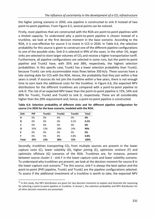
The influence of uncertainty in the development of a CO2 infrastructure
231
the higher joining scenario in 2050, one pipeline is constructed to sink D instead of two point‐to‐point pipelines. From Figure 6.5, several points can be noticed.
Firstly, most pipelines that are constructed with the ROA are point‐to‐point pipelines with a limited capacity. To understand why a point‐to‐point pipeline is chosen instead of a trunkline, we look at the first decision moment in the base scenario. According to the ROA, it is cost‐effective for source 3 to invest in CCS in 2034. In Table 6.6, the selection probability for this source is given to construct one of the different pipeline configurations to one of the possible sinks. Sink D is selected in 99% of the cases. In the other 1%, larger sinks are selected to store larger volumes of CO2 and receive a higher transportation tariff. Furthermore, all pipeline configurations are selected in some runs, but the point‐to‐point pipeline and Trunk2 have, with 35% and 38%, respectively, the highest selection probabilities. In this specific case, Trunk1 has a lower selection probability than Trunk2, because Trunk1 can only accommodate mass flows below 350 kt/y. These sources have a late starting date for CCS with the ROA. Hence, the probability that they join within a few years is small. If sources do not join the trunkline within a few years, there is not enough time to earn back the additional costs for the trunkline. In Figure 6.6, the expected NPV distributions for the different trunklines are compared with a point‐to‐point pipeline to sink D. The risk of an expected NPV lower than the point‐to‐point pipeline is 72%, 54% and 80% for Trunk1, Trunk2 and Trunk3 to sink D, respectively. These are all considerably higher than the 20% requirement and, hence, a point‐to‐point pipeline is constructed.
Table 6.6: Selection probability of different sinks and for different pipeline configuration for source 3 in 2035 for the base scenario, modeled with the ROA.
Sink PtP Trunk1 Trunk2 Trunk3 Total
A 0% 0% 0% 0% 0%
B 0% 0% 0% 0.2% 0.2%
C 0% 0% 0% 0% 0%
D 35% 13% 38% 14% 99%
E 0% 0% 0% 0% 0%
F 0% 0% 0% 0.8% 0.8%
Total 35% 13% 38% 15% 100%
Secondly, trunklines transporting CO2 from multiple sources are present in the lower capture costs (C), lower volatility (D), higher joining (E), optimistic onshore (F) and optimistic offshore (G) scenarios of the ROA. Trunklines are, for instance, present between source cluster 2 ‐ sink F in the lower capture costs and lower volatility scenario. To understand why trunklines are present, we look at the decision moment for source 8 in the lower capture cost scenario.18 For this source, sink F is always the best option and the point‐to‐point (PtP) pipeline, Trunk1 and Trunk2 are the pipeline configurations selected. To assess if the additional investment of a trunkline is worth to take, the expected NPV
18 In this study, the NPV distribution are given for two decision moments to explain and illustrate the reasoning
for selecting a point‐to‐point pipeline or trunkline. In Annex L, the selection probability and NPV distribution for all other decision moments are presented.

Chapter 6
232
distributions for Trunk1 and Trunk2 to sink F are given in Figure 6.7. The risk of a lower NPV than a point‐to‐point pipeline is 11% and 42% for Trunk1 and Trunk2, respectively. Trunk1 has a probability of less than 20% on a lower NPV than a PtP pipeline, and therefore Trunk1 is selected. The reason why in this case a trunkline is more cost‐effective than a PtP pipeline is that sources 1 and 2 want to start with CCS within 3 years, according to the ROA. As long as one of these source joins the trunkline, the trunkline is more cost‐effective than a PtP pipeline. Trunk2 is less attractive because the spare capacity of Trunk1 is already relatively large (2.5 Mt/y) and the tariff decreases with increasing capacities. For instance, for this trunkline the tariffs are 7.1 €/t and 4.8 €/t for Trunk1 and Trunk2, respectively.
Figure 6.6: Expected NPV distributions for source 3 (ammonia) for Trunk1, Trunk2 and Trunk3 to sink D for the base scenario. The red area on the left of the graph is a NPV lower and the blue area on the right a higher NPV than the point‐to‐point pipeline solution.
Thirdly, parallel pipelines are projected to be constructed in multiple ROA scenarios.19 For instance, two parallel pipelines are projected to be constructed from the landfall point to sink C in the optimistic offshore scenario. Although enough spare capacity is left in the trunkline, it was more cost‐effective for source 1 to construct an own pipeline rather than join the trunkline. To make joining cost‐effective, the tariff has to decrease with 40% (from 8.8 €/t to 5.5 €/t). This is comparable to a RRR of 8.6% instead of 16%. Note that source 1 benefits from the investment made by the previous source for developing
19 Pipelines starting from the same source cluster to the same sink (or other source cluster) are assumed to be
parallel. In Figure 6.5, they are drawn exaggerated separately from each other for clarity reasons. In reality, it is very likely that these pipelines will be placed very close to each other to make use of the same right‐of‐way.

The influence of uncertainty in the development of a CO2 infrastructure
233
surface facilities at the sink site. If no surface facilities were developed, the connection was made one year later. In the base scenario, two parallel pipelines are modelled to sink D in 2050. The reason for this is that the first source construct a point‐to‐point pipeline because the risk of the trunkline for realizing a lower NPV than the point‐to‐point pipeline was too high (>54%).
Figure 6.7: Expected NPV distributions for source 8 (PC) for Trunk1 and Trunk2 to sink F for the 30% lower capture cost scenario. The red area on the left of the graph is a NPV lower and the blue area on the right a higher NPV than the point‐to‐point pipeline solution.
Lastly, only a few of the trunklines are oversized in the ROA, see Figure 6.5. In this study, oversizing is defined as a pipeline which transports a volume that can also be handled by a diameter one size smaller. It is observed that after an oversized pipeline is constructed, it is joined almost immediately by other sources, especially the smaller ones. An exception to this is the oversized pipeline between the two source clusters in the optimistic onshore scenario in 2035, see Figure 6.5. This pipeline is constructed in 2028 with the expectation that sources 2 and 5 join the trunkline within two years. However, for these sources it is more cost‐effective to join the other trunkline. Consequently, only 18 years after construction, the pipeline capacity is fully used. This example shows that some pipelines were not correctly oversized, which is a consequence of designing a pipeline network under uncertainty.
In Table 6.7, the costs of the different layouts and the amount of CO2 stored in each scenario are given. In the base scenario, the average transport and storage costs are 13 €/t in 2050. These drop to 4.5 €/t if the capture costs are reduced with 30% and to 7.5 €/t with a 50% lower volatility. In addition, the cumulative amount of CO2 stored is projected to increase from 31 Mt to 84 Mt and 96 Mt, respectively. If only offshore storage is available, no CO2 is stored in the base scenario. In the optimistic offshore scenario, about 15% less CO2 is cumulative stored (112 Mt) than in the optimistic onshore scenario (132 Mt) in 2050. Furthermore, the average CO2 transport and storage costs are about 40% higher in the optimistic offshore (7.3 €/t) than in the optimistic onshore scenario (5.3 €/t).

Chapter 6
234
Perfect foresight and comparison with the ROA 6.5.1
The layouts of the infrastructure development are given for the perfect foresight model in Figure 6.5 and the corresponding amount of CO2 stored and costs are given in Table 6.7. A lower volatility or a higher joining probability has no effect on layout or costs of the infrastructure in the PF model. Hence, the lower volatility and higher joining scenarios are similar to the base scenario and the optimistic onshore scenario is similar to the lower capture cost scenario. Consequently, no layout or other results for these scenarios are shown. Two main observations can be made from the infrastructure projected by the PF model and their comparison with the ROA projections.
Firstly, the start of the CO2 infrastructure is projected to be developed in the onshore PF scenarios before 2025. In the offshore PF scenarios, the first sources start with capturing CO2 in 2025 and 2028. In the ROA scenarios, the development of CO2 infrastructure is projected to start 5‐10 years later. In addition, more sources start with CCS in the PF model. For example, all nine sources conduct CCS in the lower capture cost PF scenario in 2050, against six sources in the ROA. As a consequence, also more sinks are used. In the lower capture cost PF scenario, four different sinks are used and almost 60% of the overall included storage capacity is used in 2050 and almost 80% in 2060. In the optimistic offshore scenario, 70% and 100% of all available storage capacity is occupied in 2050 and 2060, respectively. Hence, the storage capacity available limits the timing and number of sources that can join the network in the optimistic offshore scenario.
Table 6.7: Costs and amount of CO2 stored for the different scenarios analyzed in this study with the PF model and ROA.a
Scenarios Cumulative amount of CO2 stored (Mt)
Cum. investment and variable costs (M€)
Cum. transport & storage costs (M€)
Average transport & storage costs (€/t CO2)
2025 2035 2050 2025 2035 2050 2025 2035 2050 2025 2035 2050
A) Base scenario
PF 0.25 46 137 58 2,283 4,446 31 306 389 124 6.7 2.8
ROA 0 0 31 0 28 1,632 0 20 410 n.a. n.a. 13
B) Only offshore
PF 0 35 109 0 1,636 3,561 0 299 678 n.a. 8.6 6.2
ROA 0 0 0 0 0 0 0 0 0 n.a. n.a. n.a.
C) Lower capture costs
PF 14 79 202 957 2,792 5,657 319 455 848 22 5.8 4.2
ROA 0 2.5 84 0 625 2,355 0 237 382 n.a. 95b
4.5
C) Lower volatility
ROA 0 18 96 0 1,394 3,730 0 428 726 n.a. 24 7.5
E) Higher joining
ROA 0 0 31 0 28 1,522 0 20 300 n.a. n.a. 9.7
F) Optimistic onshore
ROA 0 33 132 0 1,617 4,321 0 410 694 n.a. 12 5.3
G) Optimistic offshore
PF 0 46 114 0 1,338 2,716 226 299 674 n.a. 6.6 5.9
ROA 0 22 112 0 1,533 3,779 0 464 814 n.a. 21 7.3
a) No results from the PF model are given for the lower volatility and higher joining scenario, because these are similar to the base scenario. Likewise, the optimistic and the lower capture cost scenario are comparable.
b) These very high average transport and storage costs are caused by significant investments conducted just before 2035, combined with the limited amount of CO2 stored. This also explains the large drop in the average transport and storage costs of the next period.

The influence of uncertainty in the development of a CO2 infrastructure
235
Secondly, trunklines are projected to be present between the source clusters and the different sinks in all PF scenarios. None of the pipelines to the sinks transport CO2 from only one source, as was often the case in the ROA. Although not visible on the maps, oversizing pipelines happens more frequently in the PF model than in the ROA. For instance, the pipeline to sink C in the base scenario transports initially 0.25 Mt/y, but has a maximum capacity of 1.3 Mt/y. This pipeline is oversized with two sizes and remains oversized for six years. Also other several pipelines are oversized for a couple of years in the PF model, but their capacity is often fully used within a few years. In 2050, some pipelines are also oversized (like the pipeline to sink F in the lower capture cost scenario). However, these pipelines were used on full capacity in 2035. In contrast to the ROA, parallel pipelines are not present in the PF model.
From Table 6.7, it can be assessed that significant amounts of CO2 are projected to be stored with the PF model. For instance, 137 Mt is stored in the base scenario in 2050. Compared to the base PF scenario, almost 50% more CO2 is stored in the lower capture cost PF scenario, while about 20% less CO2 is stored in the only offshore scenario. Although less CO2 is stored in the only offshore scenario, the required investments in the transport and storage infrastructure increase with more than 70% compared to the base scenario. This is also reflected in the average transport and storage costs of 6.2 €/t in 2050, which is more than twice the costs of the base scenario.
Furthermore, it can be assessed that considerably less CO2 is stored in the ROA compared to the PF scenarios, see Table 6.7. For instance, in the base scenario in 2050, almost 140 Mt CO2 is projected to be cumulative captured in the PF compared to only 31 Mt in the ROA. The difference becomes smaller in the scenarios C (lower capture costs), D (lower volatility) and F (optimistic onshore). In these scenarios, 84, 96 and 132 Mt CO2 are projected to be captured with the ROA in 2050, respectively. However, this is still a difference of 30‐60% compared to related PF scenarios. Only in the optimistic offshore scenario, a similar amount of CO2 is stored, but this is caused by the lack of available storage capacity.
In the base scenario, the average transport and storage costs are more than 350% higher in the ROA than in the PF model in 2050 (see Table 6.7). The difference in average transportation and storage costs between the two approaches is smaller, with 160%; 30% and 7% in the lower volatility, optimistic onshore, and lower capture costs scenario, respectively. The difference is considerably smaller in the lower capture costs and optimistic onshore scenario, because an expensive offshore storage location needs to be opened to store the CO2 in the PF model. In general, the transport and storage costs in the ROA are considerably higher than in the PF approach, due to the less integrated network and less economies of scale.
Discussion and conclusion 6.6
In this study, the CO2 infrastructure development was modelled with two different approaches, namely a perfect foresight (PF) and a real option approach (ROA). The PF model can be considered as the optimal future, realizing the lowest cost solution for the

Chapter 6
236
entire system. In contrast, the ROA incorporates explicitly uncertainty in the CO2 price, probability that sources start with CCS and join the network, etc. Hence, the ROA reflects more the current situation, while the perfect foresight model can be a situation to strive for.
Considerations regarding the ROA and PF model 6.6.1
Similar assumptions were made for the perfect foresight model and the ROA. However, still some differences are present. Firstly, the decision to start with CCS was based on infinite lifetime in the ROA, while in the PF model the time frame till 2060 was incorporated. A shorter lifetime in the ROA would imply that sources start even later with CCS. Secondly, in the perfect foresight model it was possible to split up a mass flow between different trunklines, while in the ROA this was not possible. Thirdly, there were more starting locations for trunklines in the perfect foresight than in the ROA scenarios. The reason for this simplification in the ROA was that the underlying data of probability and willingness of joining for different kind of trunklines is completely unknown. Hence, all trunklines are assumed to start at the source and other starting locations were not incorporated for lack of data issues and simplicity reasons. Nevertheless, valuable insights are learnt from comparing the infrastructure development with and without uncertainty.
To incorporate explicitly the uncertainties in the ROA, more input data is required than for the perfect foresight model. More specifically, data is required on the volatility of the CO2 price, the tariff paid per tonne of CO2 transported, possible CCS starting dates for nearby sources, and for each of these sources the probability and willingness of joining. In particular, these last parameters are difficult to quantify and relatively simplistic assumptions were made. Nonetheless, certain trends, such as more uncertainty leading to postponement of CCS investments and less and smaller trunklines, can clearly be seen.
Considering the additional data requirements and involved effort of the ROA, a balance has to be found between applying the ROA instead of the more simple net present value (NPV) calculation and perfect foresight model. In this study, ROA is used for two decisions. First, the moment of investment is analyzed. According to Dixit and Pindyck (1994), ROA has the most added value for large initial investments, which concern an inflexible asset with large uncertainties in the future revenues and costs. Second, a decision has to be made for an appropriated sized pipeline. In our opinion, additional requirements to give ROA an added value for these kinds of decisions are economies of scale and a long time planning. Examples which would benefit from ROA include infrastructural projects (dikes, highways, bridges, etc.) and large scale technological innovations (GSM network, electric fuel stations, fiber optics, etc.). Even if there is chosen not to conduct a ROA, it has to be considered that results from the net present value calculation and perfect foresight model may be too optimistic with respect to timing, implementation rate and costs.
Summary and discussion of main results 6.6.2
Results of our case study show that 137 Mt CO2 is projected to be captured until 2050 in the PF base scenario, in comparison with 31 Mt CO2 in the ROA base scenario. In the most optimistic scenario, 132 Mt CO2 is captured up to 2050 in the ROA, compared to 202 Mt in
The influence of uncertainty in the development of a CO2 infrastructure
237
the PF model. This is still a difference of 35% between the ROA and PF model. The main reason for the significant difference in the amount of CO2 stored between PF model and the ROA is that more sources implement CCS and, in addition, they start earlier with CCS. Furthermore, in the PF model more trunklines are developed which stimulate other sources, especially smaller ones, to start also with CCS.
Less CO2 is captured in the ROA mostly because sources tend to postpone the decision to invest in CCS. The required CO2 price to stimulate CCS development almost triples in the ROA compared to the NPV approach. This required CO2 price is highly influenced by the volatility. For instance, with a volatility of 47% a pulverized coal power plant will start with CCS with a CO2 price of 99 €/t, while with a volatility of 5%, this is reduced to 47 €/t. Nonetheless, this is still 30% higher than the breakeven price of 36 €/t in the NPV approach.
An additional point to highlight is that if onshore storage is prohibited (e.g., due to public acceptance issues), CCS is only developed in an optimistic ROA scenario, meaning that the capture costs need to decrease with 30%, the volatility needs to be reduced with 50% and the joining probability is 100% for all sources. Comparing the optimistic onshore and optimistic offshore ROA scenario, about 20% less CO2 is avoided and captured up to 2050. In addition, the average transport and storage costs increase with 35% from 5.3 €/t to 7.3 €/t. In the optimistic PF scenarios, the cumulative amount of CO2 stored decrease even more, namely with 40% in 2050, if onshore CO2 storage is prohibit. The reason for this is that all offshore storage capacity is used at the end of the time frame.
With respect to the CO2 transport and storage infrastructure, clear differences could be seen between the ROA and the PF model. In the ROA, trunklines were not developed in the base scenario. Consequently, several parallel pipelines were constructed with no spare capacity. In all PF scenarios, trunklines are present and parallel pipelines are not projected. Altogether this leads to a clear difference in overall average transport and storage costs of the two approaches. For instance, for our case study, the average CO2 transport and storage in 2050 are over 4.5 times as high, namely 13 €/t instead of 2.8 €/t, in the base scenario of the ROA compared to the perfect foresight model. The difference between the two approaches is decreasing to 20% and 30% higher transport and storage costs in the optimistic offshore and optimistic onshore scenario, respectively.
The results that uncertainty leads to the postponing of investing in CCS is consistent with Abadie and Chamorro (2008), Zhou et al., (2010), Abadie et al., (2014) and Fleten and Näsäkkälä (2010). For instance, pulverized coal installations are two years later retrofitted with CCS if the CO2 price volatility increases from 2 to 5%, according to Zhou et al., (2010). Also the conclusion that much higher CO2 prices are needed to stimulate CCS development, if there is uncertainty in the CO2 price, is supported in literature (Abadie and Chamorro, 2008; Fleten and Näsäkkälä, 2010; Oda and Akimoto, 2011; Abadie et al., 2014). Abadie and Chamorro (2008) found that the required CO2 price to trigger CCS investment more than triples, with a CO2 price volatility of 47%, in comparison with the NPV approach. This is similar to the results of this study.

Chapter 6
238
Policy implications and recommendations 6.6.3
The results of this study lead to the following policy implications: ‐ Significant higher amounts of CO2 are projected to be captured and stored over the
investigated period with the PF model than with the ROA. Many future energy projections, like the ones of the IEA, do not take into account uncertainty. Hence, the amount of CO2 stored (and avoided) with CCS projected with these energy projections is probably too optimistic. This implies that to reach the projected amount of CO2 captured other measures, besides a CO2 price, will be necessary to stimulate or force companies to start with CCS. This study shows that a 30% reduction in the capture costs has a positive effect on the implementation rate of CCS. Hence, research and development to this topic should also be stimulated.
‐ The required CO2 price when companies start with CCS is highly dependent on the volatility of CO2. Even if the volatility is reduced to lower levels, the CO2 price required to stimulate investment in CCS is higher than with the standard NPV approach. Hence, policy makers should not only focus on the level of the CO2 price, but also on the uncertainty in the CO2 price.
‐ Trunklines realize economies of scale in the transportation network and stimulate CCS development, especially of smaller sources. More trunklines are developed when there is reduced uncertainty in the probability and time frame that other sources join the CO2 network. Hence, policy makers should stimulate cooperation between the different sources to facilitate trunkline development and, in this way, decrease the average transport and storage costs.
‐ If onshore CO2 storage is not allowed, the required CO2 prices to stimulate CCS development increase considerably, especially for smaller sources. Hence, policy makers should reconsider the prohibition of onshore CO2 storage, which is currently regulated in the Netherlands and Denmark. Local public opposition to CCS projects may be (partly) overcome by offering compensation to individuals or to the host community (ter Mors et al., 2012). Another possibility is to compensate companies in the additional transport and storage costs of offshore instead of onshore CO2 storage fields.
Research recommendations 6.6.4
This study was a first attempt to analyze the effect of uncertainty on the development of a CO2 infrastructure network. It can be improved by incorporating the following: ‐ Relatively large storage reservoirs were included in this study. Furthermore, a
constrain was added that the reservoir should be capable to store the CO2 of the source for minimal 20 years. It would be interesting to assess the influence (of a cluster) of small storage reservoirs without minimal storage requirements on the infrastructure layout.
‐ In this study, uncertainty was not included in every variable to limit the scope of the research. For instance, CO2 mass flows and possible capture locations may not be constant over time because existing facilities could be closed, shrink or extend their production activities. In addition, costs were assumed to be certain and fixed over

The influence of uncertainty in the development of a CO2 infrastructure
239
time, while in reality costs are uncertain and may decrease over time due to learning. Although learning is positive for the overall capture costs, it would also lead to more postponement because it gives companies an additional incentive to wait.
‐ More research is needed to come up with concrete and cost‐effective policy measures, which can stimulate CCS development under uncertain conditions.
‐ The pipeline design in this study was based on the total amount of CO2 transported in a year. In reality, the CO2 flow would vary every day (or even every hour) and the pipeline design should be based on peak flows. Consequently, the pipeline would be larger and the transportation costs will be slightly higher. Furthermore, flow variations could lead to a multi‐phase flow and the consequences of this for a CO2 network are not fully understood yet. Hence, dynamic modelling of CO2 flows deserves more attention.
References 6.7 ‐ Abadie, L.M., Chamorro, J.M., 2008. European CO2 prices and carbon capture
investments. Energy Econ 30, 2992‐3015. ‐ Abadie, L.M., Galarraga, I., Rübbelke, D., 2014. Evaluation of two alternative carbon
capture and storage technologies: A stochastic model. Environ Modell Softw 54, 182‐95.
‐ AMPL, 2014. AMPL. Streamlined modelling for real optimization. 2014. ‐ Benson, S.M., Bennaceur, K., Cook, P., Davison, J., de Coninck, H. et al., 2012. Global
Energy Assessment (GEA). Towards a sustainable future. Cambridge University Press, Cambridge UK and New York, NY, USA and the International Institute for Applied Systems Analysis, Laxenburg, Austria.
‐ Brown, D.R., Humphreys, K.K., Vail, L.W., 1993. Carbon dioxide control costs for gasification combined‐cylce plants in the United States. Prepared for the U.S. Department of Energy. PNL‐SA‐22634:1‐94.
‐ Chandel, M.K., Pratson, L.F., Williams, E., 2010. Potential economies of scale in CO2 transport through use of a trunk pipeline. Energ Convers Manage 51, 2825‐34.
‐ Chemical Engineering, 2013. Chemical plant cost index (CEPCI). Last accessed in December 2013. Retrieved from: http://www.chemengonline.com/pci‐home
‐ Chladná, Z., Chladn ý, M., Möllersten, K.,Obersteiner, M., 2004. Investment under Multiple Uncertainties: The Case of Future Pulp and Paper Mills. Interim report of the International Institute for applied systems analysis;IR‐04‐077:1‐53.
‐ Christensen, N.P., Holloway, S., 2004. Geological storage of CO2 from combustion of fossil fuel. The GESTCO project. Summary report. European Union Fifth Framework Programme for Research and Development; Second edition:1‐32.
‐ Dahowski, R.T., Dooley, J.J., Davidson, C.L., Bachu, S., Gupta, N., 2004. A CO2 storage supply curve for North America. PNWD‐3471:1‐92.
‐ Dahowski, R.T., Li, X., Davidson, C.L., Wei, N., Dooley, J.J., 2009. Regional opportunities for carbon dioxide capture and storage in China. A comprehensive CO2 storage cost curve and analysis of the potential for large scale carbon dioxide capture and storage

Chapter 6
240
in the people's Republic of China. Prepared for the U.S. Department of Energy;PNNL‐19091:1‐85.
‐ Dixit, A.K., Pindyck, R.S., 1994. Investment under uncertainty. Princeton University Press, New Jersey, U.S.A.
‐ ElementEnergy, 2010. CO2 pipeline infrastructure: An analysis of global challenges and opportunities. IEA GHG:1‐134.
‐ Energy and Environment Analysis, 2005. Characterization of the U.S. industrial/commercial boiler population. Prepared for Oak Ridge National Laboratory:1‐65.
‐ Energy Information Administration, 1995. Energy Policy Act Transportation Study: Interim Report on Natural Gas Flows and Rates. DOE/EIA‐0602(95):1‐139.
‐ Energy Information Administration, 2014. Short‐Term Energy Outlook Market Prices and Uncertainty Report. Independent Statistics & Analysis;October:1‐11.
‐ European Commission, 2011. Communication from the commission to the European parliament, the council, the European economic and social committee and the committee of the regions. A roadmap for moving to a competitive low carbon economy in 2050. COM(2011) 112 final:1‐16.
‐ Fimbres Weihs, G.A., Wiley, G.A., 2012. Steady‐state design of CO2 pipeline networks for minimal cost per tonne of CO2 avoided. Int J Greenhouse Gas Control 8, 150‐168.
‐ Fleten, S., Näsäkkälä, E., 2010. Gas‐fired power plants: Investment timing, operating flexibility and CO2 capture. Energy Econ 32, 805‐16.
‐ Fuss, S., Szolgayova, J., Obersteiner, M., Gusti, M., 2008. Investment under market and climate policy uncertainty. Appl Energy 85, 708‐21.
‐ Hacura, A., Jadamus‐Hacura, M., Kocot, A., 2001. Risk analysis in investment appraisal based on the Monte Carlo simulation technique. Eur Phys J B 20, 551‐3.
‐ Hektor, E., Berntsson, T., 2007. Future CO2 removal from pulp mills – Process integration consequences. Energ Convers Manage 48, 3025‐33.
‐ Hendriks, C., Graus, W., Van Bergen, F., 2004. Global carbon dioxide storage potential and costs. Prepared by Ecofys and TNO by order of the Rijksinstituut voor Volksgezondheid en Milieu;EEP‐02001:1‐59.
‐ Heydari, S., Ovenden, N., Siddiqui, A., 2012. Real options analysis of investment in carbon capture and sequestration technology. Comput Manag Sci 9, 109‐38.
‐ Ho, S.P., Liu, L.Y., 2002. An option pricing‐based model for evaluating the financial viability of privatized infrastructure projects. Constr Manage Econ 20, 143‐56.
‐ Hull, J.C., 1993. Options, futures, and other derivative securities. Second edition. Prentice‐Hall inc., New Jersey, U.S.A.
‐ IBM ILOG, 2015. IBM ILOG CPLEX Optimization Studio V12.6.1 Documentation. ‐ IEA, 2010. World energy outlook 2010. Organisation for Economic Co‐operation and
Development (OECD) / International Energy Agency (IEA), Paris, France. ‐ IEA, 2012. Energy Technology Perspective 2012. Pathways to a clean energy system.
Organisation for Economic Co‐operation and Development (OECD) / International Energy Agency (IEA), Paris, France.
‐ IEA, 2013a. Technology Roadmap. Carbon capture and storage. IEA publications, Paris, France.

The influence of uncertainty in the development of a CO2 infrastructure
241
‐ IEA, 2013b. World energy outlook 2013. Organisation for Economic Co‐operation and Development (OECD) / International Energy Agency (IEA), Paris, France.
‐ Johnke, B., 2002. Background papers. IPCC experts meetings on good practice guidance and uncertainty management in national greenhouse gas inventories. Institute for Global Environmental Strategies (IGES), Japan.
‐ Kato, M., Zhou, Y., 2011. A basic study of optimal investment of power sources considering environmental measures: Economic evaluation of CCS through a real option approach. Electr Eng Jpn 174, 9‐16.
‐ Knoope, M.M.J., Guijt, W., Ramírez, A., Faaij, A.P.C., 2014a. Improved cost models for optimizing CO2 pipeline configurations for point‐to‐point pipelines and simple networks. Int J Greenhouse Gas Control 22, 25‐46.
‐ Knoope, M.M.J., Raben, I., Spruijt, M., Ramírez, A., Faaij, A.P.C., 2014b. The influence of risk mitigation measures on the risk contours, costs and routing of CO2 pipelines. Int J Greenhouse Gas Control 29, 104‐24.
‐ Koller, T., Goedhart, M., Wessels, D., 2010. Valuation. Measuring and managing the value of companies. Fifth Edition. John Wiley & Sons, inc., New Jersey, USA.
‐ Kuby, M.J., Bielicki, J.M., Middleton, R.S., 2011. Optimal spatial deployment of CO2 capture and storage given a price on carbon. Int Regional Sci Rev 34, 285‐305.
‐ Kuramochi, T., Ramirez, A., Faaij, A., Turkenburg, W., 2010. Prospects for cost‐effective post‐combustion CO2 capture from industrial CHPs. Int J Greenhouse Gas Control 4, 511‐24.
‐ Kuramochi, T., Ramírez, A., Turkenburg, W., Faaij, A., 2013. Techno‐economic prospects for CO2 capture from distributed energy systems. Renew Sust Energy Rev 19, 328‐47.
‐ Kuramochi, T., Ramírez, A., Turkenburg, W., Faaij, A., 2012. Comparative assessment of CO2 capture technologies for carbon‐intensive industrial processes. Prog Energ Combust 38, 87‐112.
‐ Middleton, R.S., Bielicki, J.M., 2009. A scalable infrastructure model for carbon capture and storage: SimCCS. Energ Policy 37, 1052‐60.
‐ Middleton, R.S., Kuby, M.J., Wei, R., Keating, G.N., Pawar, R.J., 2012. A dynamic model for optimally phasing in CO2 capture and storage infrastructure. Environ Modell Softw 37, 193‐205.
‐ Mikunda, T., van Deurzen, J., Seebregts, A., Tetteroo, M., Kersemakers, K.,Apeland, S., 2011a. Towards a transport infrastructure for large‐scale CCS in Europe. Legal, financial and organizational aspects of CO2 pipeline infrastructures. CO2 Europipe;D3.3.1:1‐48.
‐ Mikunda, T., Van Deurzen, J., Seebregts, A., Kerssemakers, K., Tetteroo, M., Buit, L., 2011b. Towards a CO2 infrastructure in North‐Western Europe: Legalities, costs and organizational aspects. Enrgy Proced 4, 2409‐16.
‐ Moomaw, W., Yamba, F., Kamimoto, M., Maurice, L., Nyboer, J. et al., 2011. IPCC Special Report on Renewable Energy Sources and Climate Change Mitigation. 1st edition. Cambridge University Press, Cambridge, United Kingdom and New York, USA.
‐ Morbee, J., Serpa, J., Tzimas, E., 2012. Optimised deployment of a European CO2 transport network. Int J Greenhouse Gas Control 7, 48‐61.
Chapter 6
242
‐ Natural Gas Supply Association, 2010. Pipeline cost recovery report. 32 major pipelines. 2005‐2009. 1‐142.
‐ Neele, F., 2013. CATO2 sink database. ‐ Neele, F., 2014. Personal communication about CO2 storage in aquifers and
hydrocarbon fields in the Netherlands. ‐ Neele, F., ten Veen, J., Wilschut, F., Hofstee, C., 2012. Independent assessment of
high‐capacity offshore CO2 storage options. TNO report;TNO‐060‐UT‐2012‐00414 / B:1‐93.
‐ OANDA, 2014. Historical exchange rates. OANDA. Last accessed in August 2014. Retrieved from: http://www.oanda.com/.
‐ Oda, J., Akimoto, K., 2011. An analysis of CCS investment under uncertainty. Energy Procedia;4:1997‐2004.
‐ Oei, P., Herold, J., Mendelevitch, R., 2014. Modeling a Carbon Capture, Transport, and Storage Infrastructure for Europe. Environ Model Assess 19, 515‐31.
‐ Piessens, K., Laenen, B., Nijs, W., Mathieu, P., Baele, J.M., et al., 2008. Policy Support System for Carbon Capture and Storage. SD/CP/04A:1‐269.
‐ Piessens, K., Welkenhuysen, K., Laenen, B., Ferket, H., Nijs, W. et al., 2012. Policy Support System for Carbon Capture and Storage and collaboration between Belgium ‐ The Netherlands ‐ "PSS‐CCS". Final report. Belgian Science Policy, Brussels.
‐ Reinelt, P.S., Keith, D.W., 2007. Carbon capture retrofits and the cost of regulatory uncertainty. Energy J 28, 101‐27.
‐ Sarkis, J., Tamarkin, M., 2005. Real options analysis for "Green Trading": The case of greenhouse gases. The Engineering Economist: A Journal Devoted to the Problems of Capital Investment, 50, 273‐294.
‐ Sun, L., Chen, W., 2013. The improved ChinaCCS decision support system: A case study for Beijing–Tianjin–Hebei Region of China. Appl Energy 112, 793‐9.
‐ Switzer, L., Rosen, L., Thompson, D., Sirman, J., Howard, H., Bool, L., 2005. Carbon dioxide capture for storage in deep geological formations ‐ results from the CO2 capture project. Capture and sequestration of carbon dioxide from combustion sources. Volume I. Elsevier Ltd, The Netherlands.
‐ Szolgayova, J., Fuss, S., Obersteiner, M., 2008. Assessing the effects of CO2 price caps on electricity investments‐A real options analysis. Energy Policy 36, 3974‐81.
‐ ter Mors, E., Terwel, B.W., Daamen, D.D.L., 2012. The potential of host community compensation in facility siting. Int J Greenhouse Gas Control 11, Supplement, S130‐8.
‐ Van den Broek, M., Brederode, E., Ramírez, A., Kramers, L., van der Kuip, M. et al., 2010a. Designing a cost‐effective CO2 storage infrastructure using a GIS based linear optimization energy model. Environ Modell Softw 25, 1754‐68.
‐ Van den Broek, M., Faaij, A., Turkenburg, W., 2008. Planning for an electricity sector with carbon capture and storage. Case of the Netherlands. International Journal of Greenhouse Gas Control 2, 105‐29.
‐ Van den Broek, M., Ramírez, A., Groenenberg, H., Neele, F., Viebahn, P. et al., 2010b. Feasibility of storing CO2 in the Utsira formation as part of a long term Dutch CCS strategy: An evaluation based on a GIS/MARKAL toolbox. Int J Greenhouse Gas Control 4, 351‐66.

The influence of uncertainty in the development of a CO2 infrastructure
243
‐ Verweij, J.M., Simmelink, H.J., Van Balen, R.T., David, P., 2003. History of petroleum systems in the southern part of the Broad Fourteens Basin. Neth J Geosci 82, 71‐90.
‐ ZEP, 2011. The costs of CO2 Capture. Post‐demonstration CCS in the EU. 1‐81. ‐ Zhang, X., Wang, X., Chen, J., Xie, X., Wang, K., Wei, Y., 2014. A novel modeling based
real option approach for CCS investment evaluation under multiple uncertainties. Appl Energy 113, 1059‐67.
‐ Zhou, W., Zhu, B., Fuss, S., Szolgayová, J., Obersteiner, M., Fei, W., 2010. Uncertainty modeling of CCS investment strategy in China's power sector. Appl Energy 87, 2392‐400.
‐ Zhu, L., Fan, Y., 2011. A real options‐based CCS investment evaluation model: Case study of China's power generation sector. Appl Energy 88, 4320‐33.

244

245
Chapter 7: Summary, conclusions and recommendations
Background 7.1
One of the major challenges for the coming century is to limit drastic climate change. The parties of the United Nations Framework Convention on Climate Change agreed that long‐term global temperature should not rise more than 2°C above pre‐industrial levels (UNFCCC, 2011). It is estimated that to reach this target, CO2 emissions in the atmosphere have to stabilize on a level of 450 ppmv (Johansson et al., 2012; IEA, 2013). This implies that global CO2 emissions should peak around 2020, on a level only marginally higher than today (Riahi et al., 2012; IEA, 2014b). From then onwards, CO2 emissions should be significantly reduced.
Different options are available to limit CO2 emissions, such as renewable energy sources (wind, solar, hydro, biomass, geothermal), energy efficiency measures, switching to lower carbon intensive fuels (gas or nuclear energy) and applying carbon dioxide capture and storage (CCS). With CCS, CO2 is captured from flue gases, and subsequently transported with ships and / or pipelines to suitable underground geological storage reservoirs, like depleted hydrocarbon fields.
Most studies agree that different CO2 mitigation options are simultaneously needed to reach the required reduction of CO2 emissions (Edenhofer et al., 2010; European Commission, 2011; Riahi et al., 2012; IEA, 2013; IEA, 2014a; Bruckner et al., 2014). Compared to any other single mitigation technology, a lack of availability of CCS is most frequently associated with the most significant cost increase (Edenhofer et al., 2010; Riahi et al., 2012; Tavoni et al., 2012; Clarke et al., 2014; Krey et al., 2014). Moreover, the 2°C target becomes more difficult to reach if CCS technology is not available, especially if mitigation actions are postponed until 2030 (Edenhofer et al., 2010; Clarke et al., 2014; Riahi et al., 2015). Overall, it is projected that 9%‐38% of the primary energy mix is coupled with CCS in 2050 (Riahi et al., 2012).
Under these scenarios, up to 2050 about 55‐250 Gt CO2 needs to be captured, mainly in the industrial and power sectors (Riahi et al., 2012). To transport all the captured CO2 to suitable storage reservoirs, an extensive CO2 transportation network needs to be constructed. Currently, around 6,000‐7,000 km CO2 pipelines have been installed, mainly in the United States for enhanced oil recovery purposes (Mohitpour et al., 2012). It is expected that about 100,000 km of CO2 pipelines are needed in 2030, if CCS reaches the projected scale of 1.4 Gt CO2 avoided in 2030 (IEA, 2010). In 2050, the global network is projected to increase to an estimated length of about 200,000‐550,000 km, depending on the level of integration (IEA, 2010). To put these figures in perspective, the current high‐pressure natural gas transmission network is about 235,000 km in Europe (Marcogaz, 2011). However, while the majority of natural gas pipelines were installed within the last century, the projected CO2 pipelines should be installed within the coming decades.

Chapter 7
246
Although there are similarities between natural gas and CO2 pipeline transport, they are not one‐to‐one comparable with each other. There are knowledge gaps, among others, related to the configuration of a pipeline system, the design and operation of CO2 pipelines, the implications of impurities and consequences of safety aspects. The scope of this thesis is limited to gain insights into optimal configurations of the CO2 transportation system, including both pipeline and ship transport, and their economic consequences. The optimal pipeline configuration includes the preferred diameter, operation pressure, location of compressors and pumping stations as well as the choice between a point‐to‐point pipeline (i.e., linking one source to one sink) versus a trunkline transporting CO2 from multiple sources. The reason for focusing on the configuration of the transportation system is that this would significantly influence the costs, development and planning of a CO2 infrastructure over time. The optimal configuration can be influenced by uncertainty, safety aspects as well as by impurities. In this thesis, the implications of uncertainty and safety aspects on the costs and configuration for CO2 infrastructure development were investigated, but the consequences of impurities were not addressed.
Objective and research questions 7.2
This thesis aimed to assess, develop and test different approaches to design and evaluate cost‐effective configurations for CO2 infrastructure development. The purpose of this thesis was to generate in‐depth insights which can be used to support the development of continental, national or regional CO2 infrastructures.
In order to meet the objective, the following three research questions were formulated:
RQ 1. Which cost models are available for estimating CO2 pipeline costs, what are the key model factors driving the results, and how can the cost models be harmonized?
RQ 2. What are the most cost‐effective configurations for CO2 pipelines and networks and in what way are these affected by safety considerations?
RQ 3. Which uncertainties impact the economic viability and design of a CO2 infrastructure and how do these uncertainties influence the decision making process in the development of a CO2 transport infrastructure?
Summary of the findings per chapter 7.3
Chapter 2 provides a systematic and comprehensive overview of the existing cost models for CO2 pipelines and pumping stations available in literature. Results show that the different cost models provide a large cost range for a given pipeline diameter, especially with larger diameters. For instance, the costs for a 300 km long pipeline are estimated at 0.11‐0.64 and 1.5‐13 M€2010/km for a diameter of 0.30 m and 1.30 m, respectively. Several cost models for CO2 pipelines start with a mass flow rather than with a diameter, but also for these models a large cost range was found of, for instance, 0.9‐2.1 M€2010/km for a mass flow of 750 kg/s over 25 km. It should be realized that all costs models for pipeline transport depend, directly or indirectly, on the diameter. Therefore, also a systematic overview was made of several diameter models. This overview shows that diameter

Summary, conclusions and recommendations
247
variation is mostly caused by assumptions on the pressure drop or velocity, rather than difference in diameter models themselves. Nevertheless, if the uncertainty ranges of the diameter and cost models are combined for a given mass flow and length, the resulting cost range varies by a factor of 10. Based on the findings from the overview, key cost model characteristics were identified for a general costs comparison of CCS with other technologies and for a system analysis over time. For a general cost comparison, the cost model should at least be based on the CO2 mass flow or diameter and distance. A model used for a system analysis over time should be based on a cost model including pipeline technology, material price development, operation pressure or wall thickness, terrain impacts, effect of impurities, pipeline length and CO2 mass flow. For both applications, a pipeline cost model with parameters which have physical or economic meaning are preferred, because these models are easy to interpret and can be adjusted to new conditions. Finally, also the costs of pumping stations were studied. The findings indicate that the costs of pumping stations should be related to the capacity including some economies of scale. However, the cost range found in literature is very large, namely 3.1‐36 M€2010 for a pumping station with a capacity of 1.25 MWe. Hence, it is advised to validate the costs of pumping stations.
In chapter 3, a new cost model for CO2 pipeline transport was developed, which departed from the physical properties of CO2 transport and included different kinds of steel grades and up‐to‐date material and construction costs. The cost model was subsequently used within a new developed cost minimization tool to determine the optimal configuration for point‐to‐point pipelines and simple networks on different types of terrain and for different time frames. The cost minimization tool optimizes inlet pressure, diameter, steel grade and number of pumping stations. Results show that gaseous CO2 transport can have lower levelized costs than liquid CO2 transport for point‐to‐point pipelines as well as for simple networks from a chain perspective. Gaseous CO2 transport seems to be especially interesting for small CO2 mass flows on a close distance from a storage field with a low reservoir pressure, like a depleted gas field. The reason for this is that the lower initial compression costs compensate the higher pipeline costs. For storage reservoirs with a high reservoir pressure (like aquifers), or for CO2 transport over long distances, liquid CO2 transport is more cost‐effective than gaseous CO2 transport. For onshore pipelines transporting liquid CO2, the optimal inlet pressure is about 9‐13 MPa, pumping stations are installed roughly every 50‐100 km and higher steel grades are the most effective material (e.g., using carbon steel X120 reduces the pipeline costs up to 17% compared to X80). Most offshore pipelines and pipelines transporting gaseous CO2 do not benefit from the development of higher steel grades, due to the minimal thickness requirement. Furthermore, the results indicate that oversizing the pipeline, to transport CO2 from an additional source that is coming available later, is not always cost‐effective. This strongly depends on the time span at which additional CO2 sources are available and on the mass flows. In general, oversizing is only attractive if the second source comes available within 5‐10 years.

Chapter 7
248
Chapter 4 evaluates the implications of safety regulation on the optimal configuration, costs and routing of CO2 pipelines. For this, a quantitative risk assessment (QRA) was linked with an economic evaluation technique and a spatial model. First, the locational and societal risks of CO2 pipeline transport were calculated based on current safety regulation. Subsequently, the effect of implementing additional risk mitigation measures were assessed for the locational risks and the economic consequences of the risk mitigation measures were calculated. Finally, it was spatially determined whether rerouting or implementing additional risk mitigation measures was the most cost‐effective option. This analysis was conducted for three stylized case studies in the Netherlands, representing a point‐to‐point pipeline, a trunkline and a pipeline installed within an existing pipeline corridor. The findings indicate that dense phase CO2 pipeline transport leads to smaller lethality distances and locational risks than gaseous CO2 pipeline transport. This is caused by the large momentum behind a dense phase CO2 release, leading to a smaller but higher jet and to a higher mixing rate with the surrounding air than for a gaseous CO2 release. For instance, the 10
‐6 locational risks (i.e. the distance depicting the probability of 10‐6 per year than an unprotected ever‐present person dies) for a pipeline without additional risk mitigation measures were calculated to be 0 m for dense phase and 770 m for gaseous CO2 transport for a mass flow of about 4.5 Mt/y and a vertical release. For the gaseous case, the 10‐6 locational risks can be reduced from 770 m to 100 m if the pipeline is buried at 2.0 m depth, marker tape is installed and increased surveillance is applied. This will increase the pipeline costs with about 4%. For the dense phase cases, no additional risk mitigation measures are required to comply with Dutch regulation. Although pipelines transporting dense phase CO2 do not have 10
‐6 locational risks in our case studies, pumping stations handling about 14 MtCO2/y have a 10
‐6 locational risk distance of about 135 m. For the trunkline case, the required pumping stations could be located along the pipeline with respecting the locational risk distance. Nevertheless, it could be interesting to increase the operational pressure to avoid pumping stations, although this will increase the pipeline costs with about 20%. Based on the case studies, it can be concluded that dense phase CO2 transport is safe if it is well organized. Even without additional risk mitigation measures, the risks are manageable and within the limits established under current Dutch regulation, which is stricter or comparable with regulation in many other European countries. It is expected that pipeline route selection for dense phase CO2 transport is comparable to natural gas transport. In contrast, pipeline routing for gaseous CO2 transport appears more challenging in densely populated areas because larger safety zones are attached to it.
Chapter 5 assesses the investment decision between CO2 ship and pipeline transport by including the value of flexibility. First, the net present value (NPV) approach was applied to assess the preferred transportation mode and to evaluate if the entire CCS project, consisting of a coal power plant and offshore storage reservoir, is profitable. In the NPV approach, flexibility is neither present nor required. However, pipeline and ship transport can anticipate to uncertainties in, for instance, the CO2 price, utilization rate and volume of the storage reservoir. Different flexibility options are present to react to uncertainties. In chapter 5, the option to temporarily switch off the CO2 capture unit, the option to abandon the CCS project, and the option to connect to another storage reservoir if the

Summary, conclusions and recommendations
249
first one is full were considered. The value of each option separately and all options combined was calculated with the least‐squares Monte Carlo method, which is a real option approach (ROA). Results of the NPV and ROA show that ship transport is the most cost‐effective for transporting small volumes over long distances. For instance, for a design capacity of 2.5 Mt/y, pipelines are preferred for 250 km and ships for 500 km.
With the ROA, the option to switch to another reservoir is most valuable for the 10 MtCO2/y configurations. This option is about 10% more valuable for the pipeline than for the ship configurations with a design capacity of 10 MtCO2/y, despite the much higher switching costs of the former. The option to switch to another reservoir makes the project value positive for all considered 10 MtCO2/y configurations and pipelines are the preferred transportation mode. For smaller design capacities, the abandon option is most valuable, especially for the shipping configurations. However, the abandon option alone or combined with the other options, neither turns the project value to positive nor does it change the preferred transportation mode for design capacities of 1.0 and 2.5 MtCO2/y. For our case studies, including the value of flexibility did not change the preferred transportation mode from pipeline to ship transport. The main reasons for this are the 50% higher variable operational expenditures of ship compared to pipeline transport, combined with the fact that the other components of the shipping chain, representing about 70‐80% of the total costs, are (almost) as inflexible as pipelines. Furthermore, this analysis shows that both analyzed 10 MtCO2/y cases are profitable with the ROA, while they are not profitable with the NPV approach. Hence, incorporating the value of the most relevant flexibility options should be done to avoid that profitable projects are not conducted. The least‐squares Monte Carlo method applied in this chapter can be used to assess the value of flexibility for a range of options for different technologies.
In chapter 6, it was analyzed whether, and if so, in what way uncertainty influences the layout and costs of a CCS infrastructure, consisting of different kind of capture plants, CO2 pipelines and various storage fields. For this, two different models were developed and compared. The first model reflects the case without uncertainty and was based on perfect foresight (PF). The second model was based on the real option approach (ROA) and included uncertainties in the CO2 price, a tariff received per tonne of CO2 transported, the willingness, probability and moment that sources join the CO2 transportation network. Results show that the required CO2 price before companies make an investment in CCS almost triples in the ROA compared to the NPV approach. The required CO2 price is highly influenced by the volatility (i.e., standard deviation). For instance, with the current volatility of 47% a pulverized coal power plant will start with CCS with a CO2 price of 99 €/t, while with a volatility of 5%, this is reduced to 47 €/t. Nonetheless, this is still 30% higher than the breakeven price of 36 €/t in the NPV approach. Consequently, less sources are retrofitted with CCS and less CO2 is captured and stored over time. For instance, for the analyzed case study, 31 Mt and 137 Mt CO2 is projected to be captured in the base scenario of ROA and PF model, respectively, in the period 2015‐2050. If the volatility of the CO2 price is reduced with 50% to 23%, 96 Mt is projected to be captured in the ROA, which is still almost one third less than in the PF model. Furthermore, the results show that uncertainty leads to less development of trunklines and an increase of the number of

Chapter 7
250
point‐to‐point pipelines. All this leads to an increase of the average transport and storage costs. For our case study, the average CO2 transport and storage costs in 2050 increase from 2.9 €/t (PF model) to 13 €/t (ROA) in the base scenario. The research demonstrates the large impact that uncertainty has on the implementation rate of CCS and on the costs for developing a suitable infrastructure.
Answering the research questions 7.4
RQ 1. Which cost models are available for estimating CO2 pipeline costs, what are the key model factors driving the results, and how can the cost models be harmonized?
Fourteen different cost models for CO2 pipeline transport were identified in literature. These can be divided in five different types of cost models:
‐ Linear models ‐ Models based on the weight of the pipeline ‐ Quadratic equations ‐ CMU model, which has a Cobb Douglas format ‐ Models based on the flow rate
To compare the different cost models on a fair basis, they were harmonized by setting all terrain, regional, and other factors to 1 and the cost models were corrected to the same currency and reference year with an appropriate cost index. As a result, the costs are valid for onshore pipelines on flat terrain and are given in €2010. Subsequently, the cost models were compared with each other for a different set of diameters or mass flows, and length to assess the different cost relations.
A doubling in the diameter results in a 2 to 3.8‐fold increase of the investment costs, indicating significant economies of scale per tonne of CO2 transported. No correlation was found between length and costs for onshore pipelines as the different cost models show different relations ranging from a specific cost decrease of 10% to a cost increase of almost 18%, when the pipeline length doubles. No explanation was given, or could be found, for the specific cost increase if the length of an onshore pipeline doubles. Hence, a linear relation or minor economies of scale related to length appears to be the most appropriate relation for onshore pipelines.
For offshore pipeline transport, two opposite factors affect the relation between length and costs. Firstly, the specific pipeline costs tend to increase with pipeline length, because the inlet pressure has to increase, which requires a stronger pipeline, or the diameter has to be enlarged to compensate for the pressure drop. Secondly, there are also economies of scale related to offshore pipelines, because the costly onshore‐offshore connection has to be made only once and the equipment can be used more efficiently when laying longer pipelines.
In Figure 7.1, an overview of the costs estimated by the different costs models is given for several diameters and for an onshore pipeline of 25 km. In addition, publically available cost estimations of constructed or planned CO2 pipelines are given in Figure 7.1. The

Summary, conclusions and recommendations
251
comparison shows a very large cost range. There are three main reasons for this:
‐ Most models, except for the models based on pipeline weight, do not incorporate the higher operation pressure of the CO2 pipeline, therefore underestimating the costs
‐ Some models include the strong increase in material and construction costs of the last decade, while others do not. Although the costs are corrected with an appropriate cost index before the comparison, it is likely that still some discrepancies arise because shares between labor and material cost differ
‐ Although the terrain and regional correction factors were set to 1, some cost models are based on parameters and assumptions related to specific terrain aspects and regional circumstances.
Figure 7.1: Comparison of different cost model for CO2 pipeline transport for various diameters, based on a pipeline length of 25 km on flat terrain, with cost estimations for planned and existing CO2 pipelines. For the equations of the different models see chapter 2 and 3.
To overcome the first two shortcomings, a new cost model was developed. Our cost model is based on the weight of the pipeline, departs from the physical aspects of CO2 transport and uses recent material and construction costs. The results of this cost model for a carbon steel grade of X80 and a maximum operation pressure of 15 MPa are given in Figure 7.1. It can be concluded that our model is in the upper range of the cost models indicated in literature, with exception of the cost model of Piessens et al., (2008).
With some small adaptations, the cost model was made suitable for offshore pipeline transport. The most important modification was to include a fixed amount of 35 M€ to construct the onshore‐offshore connection and to mobilize the pipeline laying equipment.
Pipelines have to comply with the safety regulations. Additional risk mitigation measures, like marker tape, concrete sheets and block valves are available to limit the failure frequency or consequences of a pipeline failure. For dense liquid CO2 transport, additional risk mitigation measures are not required to comply with current Dutch safety regulation, which is stricter or comparable to regulation in many other European countries. Hence, under the scenarios studied, safety considerations do not appear as a key driver for costs
0.0
0.5
1.0
1.5
2.0
2.5
3.0
3.5
4.0
0.1 0.2 0.3 0.4 0.5 0.6 0.7 0.8 0.9 1.0 1.1 1.2 1.3
Costs (M
€2010/km)
Outer diameter (m)
Parker et al., 2004
Broek et al., 2010
Heddle et al., 2003
ElementEnergy, 2010
Piessens et al., 2008
Piessens et al., adapted
Gao et al., 2011
IEA GHG, 2002. ANSI 900#
IEA GHG, 2002. ANSI 1500#
McCoy and Rubin, 2008
This study, X80, 15 MPa
Alberta Carbon Trunk line
Kingsnorth CCS
Kinder Morgan
Weyburn
Denbury

Chapter 7
252
of dense liquid CO2 transport. For gaseous CO2 transport, the investment costs for onshore pipelines could increase up to about 15% to comply with safety regulation.
RQ 2. What are the most cost‐effective configurations for CO2 pipelines and networks and in what way are these affected by safety considerations?
CO2 transport cannot be evaluated on its own and should be part of a chain analysis. More specifically, the properties from the CO2 coming out of the capture plant and the storage requirements should be taken into account. Compression is often included in the CO2 capture costs, but in this thesis it was included in the transportation system, because the inlet pressure is key for optimizing the CO2 transportation system. In this thesis, a cost minimization model was developed incorporating inlet pressure, diameter, pumping stations and different kinds of steel grade to evaluate optimal configurations of CO2 pipeline transport. With this cost minimization model, it is possible to integrate the capture and transport side of CCS.
The cost minimization tool shows that gaseous CO2 transport could be an option for point‐to‐point pipelines and small scale networks if they cover only a limited length, transport a limited volume and if the CO2 is stored within a reservoir with a low bottom hole pressure, like depleted natural gas fields. A system design where gaseous CO2 of several plants is first collected and subsequently compressed with a large compressor is often less cost‐effective than immediate compression to liquid CO2 at each capture site.
Dense phase CO2 transport is the best option for pipelines and networks if they cover long lengths, transport large volumes or if the CO2 is stored within a reservoir with a high bottom hole pressure, like aquifers. For onshore pipelines transporting dense phase CO2, the optimal inlet pressure is about 9‐13 MPa and pumping stations are advised every 50‐100 km from an economic point view. Note that for offshore pipelines, pumping stations are not an option. Hence, the inlet pressure has to increase or the specific pressure drop has to decrease by increasing the pipeline diameter.
After several cost effective pipeline configurations are found for a given mass flow and length, a quantitative risk assessment (QRA) was conducted. This means that the locational risks of CO2 pipeline transport are determined, with and without several additional risk mitigation measures, like marker tape, increased surveillance, concrete slabs, etc. Subsequently, it was checked if the pipeline can be routed according to Dutch risk regulation, which state that vulnerable buildings (schools, houses, hospitals, etc.) should not be exposed to locational risks higher than 1 in the million (10‐6).
The QRA shows that safety aspects are related to gaseous CO2 transport with 10‐6
locational risk distance of, for instance, 770 m for 4.5 Mt/y and 125 m for 1.1 Mt/y for pipelines without additional risk mitigation measures. These 10‐6 locational risk distances could be decreased to 100 m and 0 m, respectively, if multiple risk mitigation measures are simultaneously applied. These additional measures increase the investment costs with 2%‐11% for the case studies analyzed. In addition, the 10‐6 locational risk distance of 100 m hampers the routing of the CO2 pipeline, at least in densely populated countries like the Netherlands. Consequently, gaseous CO2 transport is not advised for large point

Summary, conclusions and recommendations
253
sources of CO2, like coal power plants or steel factories. Overall, gaseous CO2 transport is only advised for transporting limited amounts (about <1 Mt/y) over short distances.
CO2 pipelines transporting dense phase CO2 already meets the 10‐6 locational risk distances without additional risk mitigation measures. Hence, additional risk mitigation measures are not required from a safety point of view, but some very cheap risk mitigation measures, like marker tape, could be added as part of a no‐regret strategy. In contrast to pipelines transporting dense phase CO2, pumping stations have location risk contours. For instance, pumping stations handling 14 MtCO2/y have 10
‐6 locational risks of 135 m. Although they could be placed along the pipeline route, it may be preferable to increase the inlet pressure to avoid pumping stations. An additional advantage of this solution is that pumping stations could later be added if the CO2 volume within the pipeline increases over time. This results in an additional flexibility option, which could have a considerable value.
RQ 3. Which uncertainties impact the economic viability and design of a CO2 infrastructure and how do these uncertainties influence the decision making process in the development of a CO2 transport infrastructure?
Uncertainties are present in many aspects of CCS development, like the volume of storage reservoirs, the timing when sources start with CCS, the price of CO2 and other commodities, etc. The decision to invest in (or continue with) a CCS project should be made with these uncertainties in mind.
In literature, it is standard practice to base an investment decision on the normal net present value (NPV) approach, which implies that the decision has to be taken now or never. In addition, the NPV approach assumes that revenues and costs are known over the lifetime of the project and adaptation after the investment decision is made is neither possible nor required. However, investments can be postponed to gain more information over the future and companies will adapt to changing situations. Therefore, also a real option approach (ROA) is used in this thesis, which includes the value of flexibility options, like deferring or abandoning a project.
In the initial uncertain starting up phase of CCS, ships may have an advantage compared to pipeline transport, due to their high residual value. In addition, ship transport is stated to be more flexible, because ships can easily be directed to different (storage) locations (IEA GHG, 2004; Decarre et al., 2010; Vermeulen, 2011). To investigate whether flexibility changes the preference from pipeline to ship transport, the two transportation modes were compared with each other by including the value of the option to abandon the project, switching temporarily off the capture unit and connecting to another storage reservoir. The results indicate that these options did not change the preference from pipeline to ship transport. However, the option to connect to another storage reservoir makes the project value positive for both transportation modes for a design capacity of 10 MtCO2/y and distances of 250 and 500 km.
The findings point out that especially the uncertainty in the CO2 price has a large influence on the decision to invest in a CCS project. With the historical CO2 price volatility of 47%,

Chapter 7
254
the required CO2 price before an investment in CCS is made almost triples, compared to the NPV approach. As a consequence, CCS projects are developed later in time than initially expected.
Over time, the CO2 price and the implementation rate of CCS are expected to increase, implying that the corresponding CO2 infrastructure also has to expand over time. Pipelines transporting CO2 from multiple sources in one trunkline lead to considerable economies of scale compared to an infrastructure where each source‐sink connection has a dedicated point‐to‐point pipeline. However, if the implementation rate of CCS is slower than expected, the cost‐effectiveness of trunklines declines. In the worst case, the spare capacity of trunklines is not used and becomes a ‘stranded asset’. For instance, two separate point‐to‐point pipelines transporting a similar amount of CO2 are more cost‐effective than a trunkline, if the second source is not joining the trunkline within 5 to 10 years. Hence, the rate and timing of CCS development is crucial in developing a cost‐effective infrastructure, especially if advantages from economies of scale want to be included.
To plan a cost‐effective infrastructure over time, different approaches can be taken. Existing approaches often assume perfect foresight, meaning that the infrastructure is planned with the optimized outcome in mind, without any barriers or uncertainties (among others: Van den Broek et al., 2010; Middleton et al., 2012; Morbee et al., 2012). In this way, the lowest possible costs are realized and insights are gained in attractive CO2 transport configurations. The insights of these perfect foresight models can be helpful for governments to evaluate attractive locations for trunklines and provide conditions to achieve those.
In this thesis, a different approach was developed based on the real option approach, to incorporate the fact that investment decisions are made under uncertainty about future prices, possibility that other sources start with CCS, etc. With this approach, a company perspective is adapted and it is investigated if the additional investments are worth with respect to both the expected profits and the uncertainty around the profits. By comparing investment decisions and layouts of CO2 transport with a perfect foresight model and with the real option approach, insights were gained into the effect of uncertainty on the economic viability and design of a CO2 infrastructure.
With a perfect foresight model, pipelines are oversized with multiple nominal pipe sizes, to accommodate also the CO2 flows of sources that start with CCS several years later. Especially, small CO2 emitters benefit from the presence of trunklines. In the presence of uncertainty regarding when nearby sources start with CCS, only a few companies take the risk to oversize their pipelines and only often with one nominal pipe size (so limited oversizing). Consequently, there is less surplus capacity in the pipelines and multiple smaller pipelines next to each other are thus constructed. In the absence of trunklines, many smaller CO2 emitters do not start with CCS, because the costs for constructing an own dedicated pipeline are too high. Overall, the levelized transport and storage costs increase for our regional case study from 2.9 €/t in the perfect foresight model to 13 €/t in the uncertainty scenario.

Summary, conclusions and recommendations
255
Therefore, smart strategies are required to optimally benefit from economies of scale and at the same time limit the risk of not earning back large upfront investment costs. Cooperation between companies in the same region should be stimulated, in such a way that regional networks are developed. A more integrated national, or even continental, network can most probably only be deployed if national governments, or multilateral organizations (like the European Union), play an active role in developing a CO2 infrastructure. If governments fail to stimulate cooperation, the costs of realizing a CO2 infrastructure would considerably increase.
The comparison of a scenario with and without uncertainty can be used to identify undesired developments, like the postponement of CCS investments, the development of many point‐to‐point pipelines, the presence of parallel pipelines, etc. Subsequently, these insights can be used to formulate policy measures to overcome undesired developments. The developed methodology is not only valuable for the development of a CO2 infrastructure, but can also be used to evaluate other type of (infrastructural) problems, like a glass fiber network or hydrogen infrastructure.
Final remarks 7.5
In this thesis, different approaches were developed to design and evaluate cost‐effective configurations for CO2 infrastructure development. These approaches are complementary and can be used consecutively to plan a CO2 infrastructure. First, evaluation of the profitability of CCS for companies is required, by incorporating relevant options, like abandoning or deferring the CCS project. The least‐squares Monte Carlo method or the binominal approach applied in chapter 5 and 6, respectively, can be used for this. If it is profitable to invest in CCS, cost‐effective configurations for CO2 transport have to be assessed. The cost minimization tool, which was developed in chapter 3, can be used to assess cost‐effective pipeline configurations for a given mass flow. Besides evaluating only the mass flow of one source, mass flows of nearby sources should also be incorporated to assess interesting trunkline configurations. In addition, several configurations may have almost similar levelized costs and it is recommended to also evaluate configurations, which lead to slightly higher costs, but may have other safety or flexibility advantages. Subsequently, it has to be evaluated if the different point‐to‐point pipeline and trunkline configurations comply with safety regulations, with or without additional safety measures, see chapter 4. Lastly, the different configurations, which comply with safety regulations, have to be compared with each other. As there is uncertainty in future mass flows and revenues, a Monte Carlo simulation can give insights into the profit distribution of the different configurations (see chapter 6). The configuration resulting in the highest average project value, but with a limited probability of losses, is the most interesting alternative. Communication and collaboration between different CO2 emitters would reduce the uncertainty in whether, and when, they want to join the CO2 network. This planning procedure may be influenced by policy measures and then especially the first and last step, i.e., the decision to invest in CCS and the decision to invest in a certain transport configuration.

Chapter 7
256
Before companies will invest in CCS, trust has to be gained in the technology. For this, several large scale demonstration projects covering the whole CCS chain are needed. To realize these projects, financial support is required. In this phase, point‐to‐point pipelines ‐which link one source to one sink‐ are the most appropriate. This limits the possibility of stranded assets, as it is unlikely that sources will start with CCS quickly after the start of a demonstration project. After successful demonstration, CCS technology has to be implemented rapidly in the power and industrial sector to reach the required CO2 reductions. A stable climate policy is required to persuade companies to invest in CCS technology.
In the post‐demonstration phase, developing an integrated and cost‐effective CO2 infrastructure is key to ensure that also smaller sources will start with CCS. The difficulty of realizing integrated networks is increasing from regional to national scale, because more potential sources are involved, thereby increasing the complexity of planning and managing the infrastructure development. A regional network could be realized by communication and collaboration between the different CO2 emitters in the same region, while for a national network the national government or another national organization has to play a coordinating and facilitating role. For the development of a continental network, liaising of multiple governments and potentially also coordination by a multilateral organization is required. For all geographical scales, government should facilitate trunkline development by offering compensation for the additional investment costs of trunklines compared to point‐to‐point pipelines.
The European CO2 infrastructure network is projected to be 11,000‐17,000 km in 2050 and the cumulative investments for realizing this are estimated at 15‐37 billion euros (Morbee et al., 2012). However, this estimation and many other estimations available in literature are based on a perfect foresight model. Pipeline length and investments would be considerably higher if a network, handling the same amount of CO2, is developed under uncertainty. Hence, the estimated lengths and costs, available in literature, are too optimistic for realizing a CO2 infrastructure. The real option approach, developed in chapter 5 and especially in chapter 6 of this thesis, can help with providing more realistic estimations of the length and costs of developing a CO2 infrastructure, at least when there is no strong policy in place for stimulating trunkline development.
Key research and policy recommendations 7.6
Based on the results found in the different chapters, the following recommendations for further research and policy makers are identified.
Recommendations for further research:
‐ In this thesis it was assumed that CO2 would be free of impurities (like H2S, NOx, SO2). However, impurities will be present in the CO2 flow and they would influence the phase envelope and the physical properties of CO2. Hence, they will affect the initial design and operation of transportation system. The implications of impurities in the findings of this thesis require further investigation.

Summary, conclusions and recommendations
257
‐ Optimizing the whole CCS chain is of key importance. For instance, it may be overall more cost‐effective to have very small amounts of impurities in the CO2 flow, although this increases the capture costs. Additionally, more insights have to be gained into the storage requirements (e.g., on injection temperature and pressure) of different types of storage fields over time.
‐ The pipeline system should be stable under all conditions, meaning that it has to be able to cope with variations in the mass flows due to start‐ups and (emergency) shut‐downs. The consequences of flow variations in the CO2 network are not fully understood and needs to be investigated.
‐ Before a large scale CO2 network is enrolled, the safety aspects of a large scale CO2 pipeline failure should be fully understood. This means that the toxicity of CO2 should be validated and better insights have to be gained into the entire release and dispersion of a dense phase CO2 pipeline.
‐ Uncertainty is a major hampering factor of stimulating the implementation of new technologies, like CCS, or the development of an integrated infrastructure. Hence, more research is needed to investigate cost‐effective policy measures to overcome barriers to invest in new required technologies and integrated infrastructure under uncertain (market) conditions.
Recommendations for policy makers: ‐ Policy makers should not only focus on the level of the CO2 price, but also on the
uncertainty in the CO2 price, because both influence the investment decision in CCS. In addition, other measures, besides a CO2 price, may be necessary to stimulate or force companies to start with CCS.
‐ Trunklines can offer substantial economies of scale in the transport costs and stimulate CCS development, especially for smaller CO2 emitters. Policy makers should stimulate cooperation between the different CO2 emitters to facilitate regional trunkline development and, in this way, decrease the average transport costs. For an integrated CO2 network on national or continental scale, national governments or multilateral organizations (like the European Union) should play an active role in developing a CO2 infrastructure.
‐ There is a need for several large scale demonstration projects covering the whole CCS chain for demonstrating the technology and for fully understanding the interaction between the CO2 capture plant, transport and storage facility. The projects should be selected in such a way that both ship and pipeline transport are demonstrated, thereby gaining insights into the techno‐economic aspects of linking a ship or pipeline to the injection well. In addition, these demonstration projects have to be used to acquire more knowledge about the influence of different impurity levels and the implications of dynamic flow behavior on the CO2 transportation system.
References 7.7‐ Bruckner, T., Bashmakov, I. A., Mulugetta, Y., Chum, H., de la Vega Navarro, A.,
Edmonds, J. et al., (2014). Energy Systems. In O. Edenhofer, R. Pichs‐Madruga, Y. Sokona, E. Farahani, S. Kadner, K. Seyboth, et al., (Eds.), Climate Change 2014: Mitigation of Climate Change. Contribution of Working Group III to the Fifth

Chapter 7
258
Assessment Report of Intergovernmental Panel on Climate Change. Cambridge University Press: Cambridge, United Kingdom and New York, USA.
‐ Clarke, L., Jiang, K., Akimoto, K., Babiker, M., Blanford, G., Fisher‐Vanden, K., Hourcade, J. ‐C., Krey, V., Kriegler, E., Löschel, A., McCollum, D., Paltsev, S., Rose, S., Shukla, P. R., Tavoni, M., van der Zwaan, B. C. C., & van Vuuren, D. P. (2014). Assessing Transformation Pathways. In O. Edenhofer, R. Pichs‐Madruga, Y. Sokona, E. Farahani, S. Kadner, K. Seyboth, A. Adler, I. Baum, S. Brunner, P. Eickemeier, B. Kriemann, J. Savolainen, S. Schlömer, C. von Stechow, T. Zwickel, & J. C. Minx (Eds.), Climate Change 2014: Mitigation of Climate Change. Contribution of Working Group III to the Fifth Assessment Report of Intergovernmental Panel on Climate Change.Cambridge University Press: Cambridge, United Kingdom and New York, USA.
‐ Decarre, S., Berthiaud, J., Butin, N., & Guillaume‐Combecave, J. ‐L. (2010). CO2 maritime transportation. International Journal of Greenhouse Gas Control, 4, 857‐864.
‐ Edenhofer, O., Knopf, B., Barker, T., Baumstark, L., Bellevrat, E., Chateau, B. et al., (2010). The economics of low stabilization: Model comparison of mitigation strategies and costs. Energy Journal, 31, 11‐48.
‐ European Commission (2011). Energy Roadmap 2050. Commission staff working paper. Impact Assessment, SEC(2011) 1565.
‐ IEA (2014a). Energy Technology Perspective 2014. Harnessing Electricity’s Potential. Organisation for Economic Co‐operation and Development (OECD) / International Energy Agency (IEA): Paris, France.
‐ IEA (2014b). World energy outlook 2014. Organisation for Economic Co‐operation and Development (OECD) / International Energy Agency (IEA): Paris, France.
‐ IEA (2013). World energy outlook 2013. Organisation for Economic Co‐operation and Development (OECD) / International Energy Agency (IEA): Paris, France.
‐ IEA (2010). Energy technology perspectives 2010: Scenarios and strategies to 2050. Organisation for Economic Co‐operation and Development (OECD) / International Energy Agency (IEA): Paris, France.
‐ IEA GHG (2004). Ship transport of CO2. Prepared by Mitsubishi, PH4/30, 1‐64. ‐ Johansson, T. B., Nakicenovic, N., Patwardhan, A., Gomez‐Echeverri, L., Banerjee, R.,
Benson, S. M. et al., (2012). Summaries. In T. B. Johansson, N. Nakicenovic, A. Patwardhan, & L. Gomez‐Echeverri (Eds.), Global Energy Assessment. Towards a sustainable future (pp. 3‐93). Cambridge University Press and International Institute for Applied System Analysis: Cambridge UK; New York, NY, USA; Laxenburg, Austria.
‐ Krey, V., Luderer, G., Clarke, L., & Kriegler, E. (2014). Getting from here to there ‐ energy technology transformation pathways in the EMF27 scenarios. Climatic Change, 123, 369‐382.
‐ Marcogaz (2011). Activity report 2010‐2011. Technical association of the European natural gas industry, 1‐26.
‐ Middleton, R. S., Kuby, M. J., Wei, R., Keating, G. N., & Pawar, R. J. (2012). A dynamic model for optimally phasing in CO2 capture and storage infrastructure. Environmental Modelling and Software, 37, 193‐205.

Summary, conclusions and recommendations
259
‐ Mohitpour, M., Seevam, P., Botros, K. K., Rothwell, B., & Ennis, C. (2012). Pipeline transportation of carbon dioxide containing impurities. (1st edition ed.). ASME Press: New York, USA.
‐ Morbee, J., Serpa, J., & Tzimas, E. (2012). Optimised deployment of a European CO2 transport network. International Journal of Greenhouse Gas Control, 7, 48‐61.
‐ Piessens, K., Laenen, B., Nijs, W., Mathieu, P., Baele, J. M., Hendriks, C., Bertrand, E., Bierkens, J., Brandsma, R., Broothaers, M., De Visser, E., Dreesen, R., Hildenbrand, S., Lagrou, D., Vandeginste, V., & Welkenhuysen, K. (2008). Policy Support System for Carbon Capture and Storage. SD/CP/04A, 1‐269.
‐ Riahi, K., Dentener, F., Gielen, D., Grubler, A., Jewell, J., Klimont, Z. et al., (2012). Chapter 17. Energy Pathways for Sustainable Development. In T. B. Johansson, N. Nakicenovic, A. Patwardhan, & L. Gomez‐Echeverri (Eds.), Global Energy Assessment (GEA). Towards a sustainable future. (pp. 1205‐1305). Cambridge University Press, Cambridge UK and New York, NY, USA and the International Institute for Applied Systems Analysis, Laxenburg, Austria.
‐ Riahi, K., Kriegler, E., Johnson, N., Bertram, C., den Elzen, M., Eom, J. et al., (2015). Locked into Copenhagen pledges — Implications of short‐term emission targets for the cost and feasibility of long‐term climate goals. Technological Forecasting and Social Change, 90, Part A, 8‐23.
‐ UNFCCC (2011). Report of the Conference of the Parties on its sixteenth session, held in Cancun from 29 November to 10 December 2010.Addendum Part Two: Action taken by the Conference of the Parties at its sixteenth session. Decisions adopted by the Conference of the Parties. United Nations Framework Convention on Climate Change (UNFCCC), FCCC/CP/2010/7/Add.1, 1‐31.
‐ Van den Broek, M., Brederode, E., Ramírez, A., Kramers, L., van der Kuip, M., Wildenborg, T. et al., (2010). Designing a cost‐effective CO2 storage infrastructure using a GIS based linear optimization energy model. Environmental Modelling and Software, 25, 1754‐1768.
‐ Vermeulen, T. N. (2011). Knowledge sharing report – CO2 liquid logistics shipping concept (LLSC). Overall supply chain optimization. Prepared by Tebodin B.V. for Vopak and Anthony Veder, 3112001, 1‐142.

260

261
Chapter 8: Samenvatting, conclusies en aanbevelingen
Achtergrond 8.1
Eén van de grootste uitdagingen van de komende eeuw is het voorkomen van te sterke klimaatverandering. Het klimaatverdrag van de Verenigde Naties stelt als doel dat de wereldwijde temperatuur, op de lange termijn, met niet meer dan 2°C mag stijgen (UNFCCC, 2011). Om dit doel te bereiken, zouden de CO2 emissies in de atmosfeer naar schatting moeten stabiliseren op 450 ppmv (parts per million volume) (Johansson et al., 2012; IEA, 2013). Dit betekent dat de mondiale CO2 uitstoot zou moeten pieken rond 2020 op een niveau dat slechts marginaal hoger is dan de huidige uitstoot (Riahi et al., 2012; IEA, 2014b). Vanaf 2020 zou de uitstoot van CO2 emissies significant moeten afnemen.
Er zijn verschillende opties beschikbaar om de CO2 uitstoot terug te dringen. Voorbeelden hiervan zijn hernieuwbare energiebronnen (wind, zon, water, biomassa en geothermisch), maatregelen die de energie efficiëntie verhogen, een transitie naar minder CO2 intensieve brandstoffen (gas of nucleaire energie) en het toepassen van CO2 afvang en opslag (CCS). CCS houdt in dat CO2 wordt afgevangen van rookgassen van grote industriële bronnen en vervolgens wordt getransporteerd met schepen en / of pijpleidingen naar een geschikt ondergronds opslagveld, zoals een uitgeput olie‐ of aardgasveld.
De meeste studies wijzen erop dat meerdere CO2 mitigatie opties tegelijkertijd nodig zijn om de benodigde CO2 reductie te realiseren (Edenhofer et al., 2010; European Commission, 2011; Riahi et al., 2012; IEA, 2013; IEA, 2014a; Bruckner et al., 2014). Als een mitigatie optie niet beschikbaar is zullen de kosten van CO2 reductie hoger uitvallen. Volgens de meeste studies zullen de mitigatiekosten het meeste stijgen als CCS niet beschikbaar is als CO2 mitigatie technologie (Edenhofer et al., 2010; Riahi et al., 2012; Tavoni et al., 2012; Clarke et al., 2014; Krey et al., 2014). Bovendien wordt het 2°C doel moeilijker te realiseren als CCS technologie niet inzetbaar is, vooral als mitigatie acties worden uitgesteld tot 2030 (Edenhofer et al., 2010; Clarke et al., 2014; Riahi et al., 2015). Naar schatting wordt 9‐38% van de primaire energiemix in 2050 gekoppeld met CCS technologie (Riahi et al., 2012).
Onder deze scenario’s wordt tot 2050 ongeveer 55‐250 Gt CO2 afgevangen, voornamelijk in de industriële en elektriciteitssector. Om de afgevangen CO2 te transporteren naar geschikte opslagvelden moet een uitgebreid CO2 transportnetwerk worden gebouwd. Momenteel zijn er ongeveer 6.000‐7.000 km CO2 pijpleidingen geïnstalleerd voornamelijk voor ‘enhanced oil recovery’ in de Verenigde Staten (Mohitpour et al., 2012). De schatting is dat in 2030 ongeveer 100.000 km CO2 pijpleidingen nodig zijn, mits CCS de verwachte schaal haalt van 1,4 Gt vermeden CO2 in 2030 (IEA, 2010). De lengte van het wereldwijde CO2 netwerk wordt in 2050 geraamd op ongeveer 200.000‐550.000 km, afhankelijk van de mate van integratie (IEA, 2010). Om deze getallen in perspectief te plaatsen: de lengte van het huidige Europees transmissienetwerk voor aardgas op hoge druk is ongeveer 235.000 km (Marcogaz, 2011). De meerderheid van deze aardgasleidingen zijn echter

Chapter 8
262
aangelegd in de laatste eeuw, terwijl het geraamde CO2 netwerk in de komende decennia moet worden gebouwd.
Hoewel er overeenkomsten zijn tussen aardgas en CO2 pijpleidingtransport, zijn ze niet één op één met elkaar te vergelijken. Er zijn verschillende kennishiaten in onder andere de configuratie van het pijpleidingsysteem, het ontwerp en de operationele aspecten van CO2 pijpleidingen, de consequenties van onzuiverheden en veiligheidsaspecten. Dit proefschrift beperkt zich tot het verwerven van inzichten in de optimale configuraties en de economische aspecten van het CO2 transportsysteem bestaande uit zowel pijpleiding‐ als schiptransport. Voor de optimale pijpleidingconfiguratie worden de voorkeursdiameter, operationele druk, locatie van compressie‐ en pompstations meegenomen alsmede de keuze tussen een punt‐naar‐punt pijpleiding (i.e., de verbinding tussen één bron en één opslagveld) en een trunkline, die CO2 transporteert van meerdere bronnen. Deze studie richt zich op de transportsysteemconfiguratie omdat deze over de tijd grote impact heeft op de kosten, ontwikkeling en planning van een CO2 infrastructuur. De optimale configuratie kan beïnvloedt worden door onzekerheden, veiligheidsaspecten en onzuiverheden. In dit proefschrift zijn de gevolgen van onzekerheden en veiligheidsaspecten op de ontwikkeling en configuratie van CO2 infrastructuur onderzocht. De gevolgen van onzuiverheden zijn echter buiten beschouwing gelaten.
Doelstelling en onderzoeksvragen 8.2
Het doel van dit proefschrift is om methoden te analyseren, ontwikkelen en testen, voor het ontwerp, ontwikkeling en evaluatie van kosteneffectieve configuraties van CO2
infrastructuren en hoe deze kennis de ontwikkeling van CO2 infrastructuur op continentale, nationale en regionale schaal kan faciliteren.
Om de doelstelling te beantwoorden, zijn de volgende drie onderzoeksvragen geformuleerd:
OV 1. Welke kostenmodellen zijn beschikbaar voor het schatten van de kosten van CO2 pijpleidingen, wat zijn de belangrijkste modelfactoren die de kosten bepalen en hoe kunnen de kostenmodellen worden geharmoniseerd?
OV 2. Wat zijn meest kosteneffectieve configuraties voor CO2 pijpleidingen en netwerken en op welke manier veranderen deze door veiligheidsaspecten?
OV 3. Welke onzekerheden hebben invloed op de economische levensvatbaarheid en ontwerp van een CO2 infrastructuur en hoe beïnvloeden deze onzekerheden het besluitvormingsproces in de ontwikkeling van een CO2 transportinfrastructuur?
Samenvatting van de resultaten per hoofdstuk 8.3
Hoofdstuk 2 geeft een systematische en beknopt literatuuroverzicht van de kostenmodellen voor CO2 pijpleidingen en pompstations. De verschillende kostenmodellen geven een grote kostenrange voor alle pijpleidingen maar met name voor leidingen met een grote diameter. Om een voorbeeld te geven, de kosten voor een

Samenvatting, conclusies en aabevelingen
263
300 km lange pijpleiding worden geschat op 0,11‐0,64 miljoen euro per kilometer (M€2010/km) voor een diameter van 0,30 m en op 1,5‐13 M€2010/km voor een diameter van 1,30 m. Er zijn ook een aantal kostenmodellen voor CO2 pijpleidingen beschikbaar die gebaseerd zijn op de CO2 massastroom in plaats van op de diameter. Maar ook bij deze kostenmodellen is de range groot, namelijk van 0,9‐2,1 M€2010/km voor een massastroom van 750 kg/s over 25 km. Omdat alle kostenmodellen voor pijpleidingtransport direct of indirect gebaseerd zijn op de pijpleidingdiameter is er een literatuuroverzicht gemaakt van de verschillende diametermodellen. Dit overzicht toont aan dat verschillende diametermodellen nauwelijks invloed hebben op de diametervariatie. De diametervariatie wordt voornamelijk veroorzaakt door verschillende aannames in de drukval of snelheid van de CO2 stroom. Vervolgens zijn de onzekerheidsintervallen van de verschillende diameter‐ en kostenmodellen voor een specifieke massastroom en lengte gecombineerd. Dit leidt tot een verschil in de minimale en maximale kosten van een factor 10.
Gebaseerd op de uitkomsten van het literatuuroverzicht zijn de belangrijkste modelfactoren in kaart gebracht voor twee verschillende doeleinden. Het eerste doeleinde is om een algemene kostenvergelijking van CCS met andere technologieën te maken en het tweede om een systeemanalyse over de tijd te doen. Een kostenmodel dat gebruikt wordt voor een algemene kostenvergelijking moet in ieder geval gebaseerd zijn op de lengte en de CO2 massastroom of diameter. Een kostenmodel voor een systeemanalyse over de tijd zou de pijpleidingtechnologie, de ontwikkeling van materiaalprijzen, operationele druk of dikte van de pijpleiding, terreinaspecten, effecten van onzuiverheden, lengte en CO2 massastroom moeten meenemen. De voorkeur gaat voor beide toepassingen uit naar een kostenmodel voor CO2 pijpleidingtransport waarin de parameters een fysische of economische betekenis hebben. Dit type modellen is makkelijker te interpreteren en aan te passen aan nieuwe condities. De bevindingen laten verder zien dat dat de kosten voor pompstations zouden moeten worden gerelateerd aan de capaciteit van het pompstation. Ook zou het kostenmodel enige schaalvoordelen voor pompstations met een grote capaciteit moeten meenemen. De kostenrange die gevonden is in de literatuur is echter erg groot, namelijk 3,1‐36 M€2010 voor een pompstation met een capaciteit van 1,25 MWe. Daarom is verdere validatie van de kosten van pompstations noodzakelijk.
In hoofdstuk 3 is een nieuw kostenmodel voor CO2 pijpleidingtransport ontwikkeld. Dit kostenmodel start met de fysische eigenschappen van CO2 transport, neemt verschillende staalkwaliteiten mee en is gebaseerd op recente materiaal‐ en constructiekosten. Het kostenmodel is vervolgens gebruikt als input voor een nieuw ontwikkeld kostenminimalisatiemodel. Het kostenminimalisatiemodel bepaalt de optimale configuratie voor punt‐naar‐punt pijpleidingen en voor simpele transportnetwerken over verschillende terreintypes en voor verschillende tijdsperiodes. In het model worden de ingangsdruk, diameter, staalkwaliteit en aantal pompstations geoptimaliseerd. De resultaten laten zien dat gasvormig CO2 transport vanuit een ketenperspectief lagere kosten per ton CO2 kan hebben dan vloeibaar CO2 transport voor punt‐naar‐punt pijpleidingen en voor simpele transportnetwerken. CO2 transport in de gasfase lijkt met name interessant te zijn voor het transport van kleine CO2 massastromen die vrijkomen

Chapter 8
264
op een korte afstand van een opslagveld met een lage reservoirdruk, bijvoorbeeld een leeg aardgasveld. De reden hiervoor is dat de hogere pijpleidingkosten worden gecompenseerd door de lagere kosten voor initiële compressie. Transport van vloeibaar CO2 is kosteneffectiever dan van gasvormig CO2 naar opslagvelden met een hoge reservoirdruk (zoals aquifers) of over lange afstanden. De optimale ingangsdruk voor pijpleidingen op land die vloeibaar CO2 transporteren is ongeveer 9‐13 MPa, pompstations zijn ruwweg elke 50‐100 km nodig en qua materiaal kan het beste gebruik worden gemaakt van hogere staalkwaliteiten (e.g., het gebruik van koolstofstaal X120 reduceert de pijpleidingskosten tot 17% in vergelijking met X80). De meeste pijpleidingen op zee en pijpleidingen die gasvormig CO2 transporteren profiteren niet van de ontwikkeling van staalsoorten met een hogere kwaliteit door de minimale dikte eis. De resultaten tonen verder aan dat overdimensionering van pijpleidingen, om te anticiperen op grotere toekomstige CO2 stromen, niet altijd kosteneffectief is. De kosteneffectiviteit van overdimensionering hangt sterk samen met de tijd waarna extra CO2 bronnen beschikbaar komen en met de hoeveelheid CO2 van die bronnen. Over het algemeen is overdimensionering alleen aantrekkelijk als een tweede CO2 bron binnen 5‐10 jaar beschikbaar komt.
Hoofdstuk 4 evalueert de gevolgen van veiligheidsvoorschriften voor de optimale configuratie, kosten en route van CO2 pijpleidingen. Hiervoor is een kwantitatieve risicoanalyse gecombineerd met een economische evaluatiemethode en een ruimtelijk model. Eerst zijn, op basis van de huidige veiligheidsvoorschriften, de plaatsgebonden‐ en groepsrisico’s van CO2 pijpleidingtransport berekend. Vervolgens zijn de effecten van extra risico mitigerende maatregelen op het plaatsgebonden risico geanalyseerd en de economische consequenties van deze maatregelen berekend. Als laatste wordt ruimtelijk bekeken of het kostenefficiënter is om de route van de pijpleiding te veranderen of om extra risico mitigerende maatregelen te implementeren. Deze analyse is gedaan voor drie casestudies in Nederland. Deze casestudies vertegenwoordigen een punt‐naar‐punt pijpleiding, een zogenaamde trunkline die CO2 transporteert van meerdere bronnen, en een pijpleiding geïnstalleerd in een bestaande pijpleidingenstraat. De uitkomsten wijzen erop dat CO2 pijpleidingtransport in de vloeibare fase leidt tot kleinere letaliteitsafstanden en plaatsgebonden risico’s dan CO2 pijpleidingtransport in de gasfase
1. Dit wordt veroorzaakt door het grote momentum van een vloeibare CO2 uitstroom, welke leidt tot een kleinere maar hogere pluim en grotere mengratio met de omliggende lucht dan voor een gasvormige CO2 uitstroom. De 10‐6 plaatsgebonden risico’s van een pijpleiding zonder extra risico mitigerende maatregelen zijn bijvoorbeeld berekend op 0 m voor vloeibaar CO2 en 770 m voor gasvormig CO2 transport met een massastroom van 4,5 Mt/jaar en een verticaal georiënteerde uitstroom2. De 10‐6 plaatsgebonden risico’s kunnen voor de gasvormige casus worden gereduceerd van 770 m tot 100 m als de pijpleiding begraven
1 Vloeibaar CO2 verwijst in dit hoofdstuk naar CO2 dat vloeibaar is gemaakt door het op druk te brengen van de CO2. 2 Een 10
‐6 plaatsgebonden risico laat de afstand zien waarop de jaarlijkse overlijdenskans van een persoon die
zich continu en onbeschermd op een bepaalde plaats bevindt, één op de miljoen (10‐6) is.

Samenvatting, conclusies en aabevelingen
265
wordt op een diepte van 2,0 m, waarschuwingslint wordt geïnstalleerd en extra surveillance wordt toegepast. Dit verhoogt de kosten van de pijpleiding met ongeveer 4%. Er zijn geen extra risico mitigerende maatregelen nodig voor de vloeibare casussen om te voldoen aan de Nederlandse voorschriften. In onze casestudies hebben pijpleidingen die vloeibaar CO2 transporteren geen 10
‐6 plaatsgebonden risico’s maar pompstations die circa 14 MtCO2/jaar behandelen hebben 10
‐6 plaatsgebonden risico’s van circa 135 m. Rekening houdend met het plaatsgebonden risico kunnen de benodigde pompstations worden geplaatst langs de trunkline. Desalniettemin zou het interessant kunnen zijn om de operationele druk in de trunkline te verhogen om zo het aantal pompstations terug te dringen of in zijn geheel te voorkomen. Dit laatste zou de pijpleidingkosten met ongeveer 20% verhogen. Gebaseerd op de uitgevoerde casestudies kan worden geconcludeerd dat vloeibaar CO2 transport veilig is, mits het goed georganiseerd is. Zelfs zonder extra risico mitigerende maatregelen zijn de risico’s hanteerbaar en binnen de grenzen die vastgesteld zijn onder de Nederlandse voorschriften, welke strikter of vergelijkbaar is met de voorschriften in veel andere Europese landen. Er wordt verwacht dat de routebepaling van vloeibaar CO2 transport vergelijkbaar is met aardgastransport. De routebepaling voor gasvormig CO2 transport lijkt echter een grotere uitdaging te vormen in dichtbevolkte gebieden omdat gasvormig CO2 transport grotere veiligheidsafstanden heeft.
Hoofdstuk 5 analyseert de investeringsbeslissing tussen CO2 schip‐ en pijpleidingtransport en houdt daarbij rekening met de waarde van flexibiliteit. De netto contante waarde (NCW) methode wordt eerst toegepast om de voorkeur tussen schip en pijpleiding te bepalen en om te evalueren of het gehele CCS project, bestaande uit een kolencentrale en een opslagreservoir op zee, winstgevend is. In de NCW methode is flexibiliteit niet aanwezig en ook niet nodig. Pijpleiding‐ en schiptransport kunnen echter anticiperen op onzekerheden in bijvoorbeeld de CO2 prijs, de capaciteitsfactor van de kolencentrale en het volume van het opslagveld. Er zijn verschillende flexibiliteitsopties aanwezig om te reageren op onzekerheden. In hoofdstuk 5 zijn drie opties geanalyseerd, namelijk de optie om tijdelijk de CO2 afvang installatie uit te schakelen, de optie om te stoppen met het CCS project en de optie om naar een ander opslagveld te gaan als het eerste opslagveld vol is. De waarde per optie en van alle opties samen zijn berekend met de kleinste kwadraten Monte Carlo methode. Dit is een reële optie methode (ROA). Resultaten van de NCW en ROA laten zien dat schiptransport het meest kosteneffectief is voor CO2 transport van kleine hoeveelheden over grotere afstanden. Om een voorbeeld te geven, voor een ontwerpcapaciteit van 2,5 Mt/jaar geniet pijpleidingtransport de voorkeur bij een afstand van 250 km en schiptransport bij een afstand van 500 km.
Volgens de ROA is de meest waardevolle optie voor de 10 MtCO2/jaar configuraties om naar een ander opslagveld te gaan als het eerst opslagveld vol is. Deze optie is voor een ontwerpcapaciteit van 10 MtCO2/jaar circa 10% meer waard voor de pijpleiding‐ dan voor de schipconfiguratie, ondanks de veel hogere kosten on naar een ander opslagveld te gaan voor de pijpleidingconfiguraties. De optie om te switchen naar een ander opslagveld maakt de projectwaarde positief voor alle geanalyseerde 10 MtCO2/jaar configuraties. Pijpleidingtransport geniet hierbij de voorkeur boven schiptransport. De optie om te stoppen met het project is het waardevolst voor kleinere ontwerpcapaciteiten, en dit

Chapter 8
266
geldt met name voor de schipconfiguraties. Deze optie is echter noch alleen, noch gecombineerd met de andere opties, genoeg om de projectwaarde positief te maken of om de voorkeur schip‐ en pijpleidingtransport te veranderen voor ontwerpcapaciteiten van 1,0 en 2,5 MtCO2/jaar. De voorkeur voor onze casestudies verandert niet van pijpleiding‐ naar schiptransport door het meenemen van de waarde van flexibiliteit. De belangrijkste redenen hiervoor zijn dat de variabele kosten van schepen 50% hoger zijn dan voor pijpleidingen en het feit dat de andere componenten van de schipketen, welke circa 70‐80% van de kosten vertegenwoordigen, (bijna) net zo inflexibel zijn dan pijpleidingen. De analyse laat verder zien dat beide 10 MtCO2/jaar configuraties winstgevend zijn met de ROA, terwijl ze niet winstgevend zijn met de NCW methode. De waarde van de belangrijkste flexibiliteitsopties zou dus moeten worden meegenomen om te voorkomen dat projecten die winstgevend zijn toch niet worden uitgevoerd, omdat de NCW negatief is. De kleinste kwadraten Monte Carlo methode die toegepast is in dit hoofdstuk kan worden gebruikt om de waarde van flexibiliteit van verschillende opties voor verschillende technologieën te analyseren.
In hoofdstuk 6 is geanalyseerd of, en zo ja in welke mate, onzekerheid de lay‐out en kosten beïnvloedt van een CCS infrastructuur. De CCS infrastructuur in dit hoofdstuk bestaat uit verschillende type CO2 bronnen, pijpleidingen en opslagvelden. Er zijn twee verschillende modellen ontwikkeld en met elkaar vergeleken om de invloed van onzekerheid te analyseren. Het eerste model reflecteert een case zonder onzekerheid en is gebaseerd op een situatie met volledige voorkennis, een zogenaamd ‘perfect foresight’ (PF) model. Het tweede model is gebaseerd op de reële optie theorie (ROA). Dit ROA model neemt onzekerheden in de CO2 prijs, het tarief per ton CO2 dat getransporteerd wordt en het moment waarop, de kans en bereidheid dat bronnen zich aansluiten op het CO2 transport netwerk mee. De resultaten laten zien dat de benodigde CO2 prijs, voordat bedrijven een investering maken in CCS, bijna verdrievoudigd met de ROA in vergelijking met de NCW methode. De benodigde CO2 prijs is sterk afhankelijk van de volatiliteit (i.e., standaard afwijking) in de CO2 prijs. Om een voorbeeld te geven, een poederkoolcentrale zal, gegeven de huidige volatiliteit van 47%, beginnen met CCS bij een CO2 prijs van 99 €/t terwijl de benodigde CO2 prijs zakt naar 47 €/t in het geval van een volatiliteit van 5%. Desondanks is dit nog steeds 30% hoger dan de break‐even prijs van 36 €/t van de NCW methode. Dit betekent in de praktijk dat er minder bronnen worden uitgerust met CCS en dat er minder CO2 wordt afgevangen en opgeslagen over de tijd. In de geanalyseerde casestudie wordt bijvoorbeeld gedurende de periode 2015‐2050 volgens het base scenario van de ROA naar verwachting 31 Mt CO2 afgevangen. Volgens het base scenario van het PF model is dit 137 Mt CO2. Als de volatiliteit van de CO2 prijs afneemt met 50% tot 23%, dan wordt er naar verwachting 96 Mt afgevangen in de ROA. Dit is nog steeds bijna 1/3 minder dan met het PF model. De resultaten laten verder zien dat onzekerheid tot minder trunklines leidt en tot een stijging van het aantal punt‐naar‐punt pijpleidingen. Dit alles tezamen resulteert in een stijging van de gemiddelde transport‐ en opslagkosten. De gemiddelde CO2 transport‐ en opslagkosten nemen voor onze casestudie toe van 2,9 €/t (PF model) tot 13 €/t (ROA) in het base scenario in 2050. Dit onderzoek demonstreert de grote impact die onzekerheid heeft op de implementatiegraad van CCS en op de kosten om een geschikte infrastructuur te ontwikkelen.

Samenvatting, conclusies en aabevelingen
267
Beantwoording van de onderzoeksvragen 8.4
OV 1. Welke kostenmodellen zijn beschikbaar voor het schatten van de kosten van CO2 pijpleidingen, wat zijn de belangrijkste modelfactoren die de kosten bepalen en hoe kunnen de kostenmodellen worden geharmoniseerd?
Er zijn veertien verschillende kostenmodellen voor CO2 pijpleidingtransport in de literatuur geïdentificeerd. Deze kunnen worden onderverdeeld in vijf verschillende type kostenmodellen:
‐ Lineaire kostenmodellen ‐ Kostenmodellen gebaseerd op het gewicht van de pijpleiding ‐ Kwadratische vergelijkingen ‐ CMU model, die een Cobb Douglas vergelijking volgt ‐ Kostenmodellen gebaseerd op de massastroom
De verschillende kostenmodellen zijn geharmoniseerd om een eerlijke vergelijking mogelijk te maken. Dit houdt in dat alle terrein, regionale en andere factoren op 1 zijn gezet. Verder zijn de kosten gecorrigeerd met een geschikte kostenindex zodat alle kosten uitgedrukt worden in dezelfde geldeenheid en referentiejaar. Na de harmonisatie geven alle kostenmodellen de kosten in €2010 voor pijpleidingen op land over vlak terrein. Vervolgens worden de kostenmodellen met elkaar vergeleken voor verschillende lengtes en diameters of massastromen. Ten slotte zijn de verschillende onderliggende kostenrelaties geanalyseerd.
Een verdubbeling van de diameter leidt tot 2 tot 3,8 keer zo hoge investeringskosten. Dit wijst op significante schaalvoordelen per ton getransporteerde CO2. Er is geen eenduidige correlatie tussen de lengte en kosten van pijpleiding op land. De verschillende kostenmodellen laten, bij verdubbeling van de lengte van de pijpleiding, namelijk relaties zien die variëren van een kostendaling van 10% tot een kostenstijging van bijna 18% per kilometer pijpleiding. Voor het fenomeen van een kostenstijging kon in de geraadpleegde literatuur geen verklaring worden gevonden. Zodoende lijkt een lineaire kostenrelatie of een kostenrelatie met een bescheiden schaalvoordeel het meest geschikt voor pijpleidingen op land.
Twee tegengestelde effecten beïnvloeden de relatie tussen lengte en kosten voor pijpleidingen op zee. Het eerste effect laat de kosten per kilometer pijpleiding stijgen als de pijpleidinglengte toeneemt. Dit wordt veroorzaakt doordat de diameter moet worden vergroot om het drukverlies per kilometer te verkleinen of doordat de ingangsdruk moet worden verhoogd wat een sterkere pijpleiding vereist. Het tegengestelde effect wordt veroorzaakt door schaalvoordelen gerelateerd met de aanleg van pijpleidingen op zee. Dit wordt veroorzaakt doordat de kostbare land ‐ zee verbinding maar één keer hoeft te worden aangelegd en doordat het materieel dat nodig is om pijpleidingen aan te leggen op zee efficiënter kan worden gebruikt.
Figuur 8.1 geeft een overzicht van de kosten die geschat zijn door de verschillende kostenmodellen voor een 25 km lange pijpleiding op land met verschillende diameters. Daarnaast zijn er verschillende openbare kostenschattingen van bestaande of geplande

Chapter 8
268
CO2 pijpleidingen weergegeven in Figuur 8.1. Het overzicht laat een grote kostenrange zien voor een bepaalde diameter. Daar zijn drie hoofdredenen voor:
‐ De meeste kostenmodellen, behalve de kostenmodellen die gebaseerd zijn op het gewicht van de pijpleiding, nemen niet mee dat CO2 pijpleidingen opereren onder een hogere druk dan aardgaspijpleidingen. Hierdoor onderschatten ze de kosten.
‐ Sommige kostenmodellen nemen de sterke stijging van de materiaal‐ en aanlegkosten mee van het laatste decennium, terwijl andere dit niet doen. Alhoewel de kosten gecorrigeerd zijn met een geschikte kostenindex voor de vergelijking, is het waarschijnlijk dat er nog steeds verschillen zitten tussen de modellen die dit wel en niet meenemen door de verschillende fracties van arbeids‐ en materiaalkosten in de verschillende kostenmodellen en gebruikte index.
‐ Sommige kostenmodellen zijn op parameters en aannames van specifieke terrein en regionale omstandigheden gebaseerd, ondanks dat alle terrein en regionale correctiefactoren op 1 zijn gezet.
Figuur 8.1: Vergelijking van de verschillende kostenmodellen van CO2 pijpleidingtransport voor verschillende diameters, gebaseerd op een 25 km lange pijpleiding op land over vlak terrein. Daarnaast zijn openbare kostenschatting van bestaande en geplande CO2 pijpleidingen opgenomen. De vergelijkingen van de verschillende modellen kunnen worden teruggevonden in hoofdstuk 2 en 3.
Er is een nieuw kostenmodel ontwikkeld om de eerste twee tekortkomingen aan te pakken. Ons kostenmodel is gebaseerd op het gewicht van de pijpleiding, start met de fysische eigenschappen van CO2 transport en gebruikt recente kostendata voor materiaal‐ en aanlegkosten. De resultaten van dit kostenmodel zijn voor koolstofstaal X80 en een maximale operationele druk van 15 MPa weergegeven in Figuur 8.1. Uit de grafiek kan worden afgeleid dat ons kostenmodel een relatief hoge kostenschatting geeft in vergelijken met de andere kostenmodellen, met uitzondering van het kostenmodel van Piessens et al. (2008).
0,0
0,5
1,0
1,5
2,0
2,5
3,0
3,5
4,0
0,1 0,2 0,3 0,4 0,5 0,6 0,7 0,8 0,9 1,0 1,1 1,2 1,3
Costs (M
€2010/km)
Outer diameter (m)
Parker et al., 2004
Broek et al., 2010
Heddle et al., 2003
ElementEnergy, 2010
Piessens et al., 2008
Piessens et al., adapted
Gao et al., 2011
IEA GHG, 2002. ANSI 900#
IEA GHG, 2002. ANSI 1500#
McCoy and Rubin, 2008
This study, X80, 15 MPa
Alberta Carbon Trunk line
Kingsnorth CCS
Kinder Morgan
Weyburn
Denbury

Samenvatting, conclusies en aabevelingen
269
Het ontwikkelde kostenmodel kan met een aantal kleine aanpassingen geschikt worden gemaakt voor pijpleidingtransport op zee. De belangrijkste aanpassing is de toevoeging van een vast bedrag van 35 M€ om de land‐zee connectie te realiseren en om het materieel te mobiliseren dat nodig is om pijpleidingen op zee aan te leggen.
Pijpleidingen moeten voldoen aan veiligheidsvoorschriften. Bestaande risico mitigerende maatregelen, zoals waarschuwingslint, betonnen beschermplaten en afsluitkleppen, zijn beschikbaar om de faalkans te verkleinen of om de consequenties van een pijpleidingongeluk te beperken. Extra risico mitigerende maatregelen zijn voor vloeibaar CO2 transport niet noodzakelijk om aan de Nederlandse richtlijnen te voldoen, welke vergelijkbaar of strikter zijn met de richtlijnen van veel andere verschillende Europese landen. Onder de bestudeerde scenario’s, lijken veiligheidsaspecten daarom geen belangrijke kostenbepalende factor te zijn voor CO2 transport in de vloeibare fase. De investeringskosten voor pijpleidingen die gasvormig CO2 transport vervoeren over land kunnen met maximaal circa 15% stijgen om aan de veiligheidsvoorschriften te voldoen.
OV 2. Wat zijn meest kosteneffectieve configuraties voor CO2 pijpleidingen en netwerken en op welke manier veranderen deze door veiligheidsaspecten?
CO2 transport kan niet als losstaand onderdeel worden geanalyseerd en moet deel uitmaken van een ketenanalyse. Zo moeten de eigenschappen van de CO2 uit de afvanginstallatie en de eisen van het opslagveld worden meegenomen. De kosten van het op druk brengen van de CO2 vallen vaak onder de CO2 afvangkosten. In dit proefschrift worden deze echter meegenomen in het transportsysteem omdat de ingangsdruk belangrijk is om het CO2 transportsysteem te optimaliseren. Er is in dit proefschrift een kostenminimalisatiemodel ontwikkeld die de ingangsdruk, diameter, pompstations en verschillende staalkwaliteiten meeneemt om tot optimale configuraties voor CO2 pijpleidingtransport te komen. Met dit kostenminimalisatiemodel is het mogelijk om de afvanginstallatie en het transportsysteem met elkaar te integreren.
Het kostenminimalisatiemodel laat zien dat CO2 transport in de gasfase een optie kan zijn voor punt‐naar‐punt pijpleidingen en voor kleinschalige transportnetwerken die een geringe lengte beslaan, een beperkt volume transporteren en de CO2 opslaan in een opslagveld met een lage reservoirdruk, zoals een uitgeput aardgasveld. Een ontwerp waarbij gebruik wordt gemaakt van een verzamelpunt om gasvormige CO2 van verschillende afvanglocaties te comprimeren naar vloeibare CO2 is vaak minder kostenefficiënt dan een ontwerp waarbij de CO2 bij elke opvanglocatie afzonderlijk gecomprimeerd wordt. CO2 transport in de vloeibare fase is meestal de beste optie voor pijpleidingen en pijpleidingnetwerken als ze een lange lengte hebben, grote volumes transporteren of als de CO2 opgeslagen wordt in een opslagveld met een hoge reservoirdruk, zoals aquifers. Voor pijpleidingen op land die vloeibaar CO2 vervoeren, is de optimale druk circa 9‐13 MPa en de adviesafstand tussen pompstations, vanuit een economisch perspectief, is 50‐100 km. Pompstations zijn geen optie voor pijpleidingen op zee en daarom moet de ingangsdruk worden verhoogt of moet de specifieke drukval worden verlaagt. Dit laatste kan door het vergroten van de diameter van de pijpleiding worden gerealiseerd.

Chapter 8
270
Nadat verschillende kosteneffectieve pijpleidingconfiguraties voor een specifieke massastroom en lengte zijn gevonden, is een kwantitatieve risicoanalyse uitgevoerd. Dit betekent dat de plaatsgebonden risico’s voor CO2 pijpleidingtransport worden berekend met en zonder verschillende risico mitigerende maatregelen zoals waarschuwingslint, extra surveillance, betonnen beschermplaten etc. Vervolgens is onderzocht of de pijpleidingroute kan worden bepaalt met inachtneming van de Nederlandse veiligheidsvoorschriften. Deze voorschriften stellen dat kwetsbare objecten (zoals scholen, huizen, ziekenhuizen etc.) niet mogen worden blootgesteld aan plaatsgebonden risico’s boven 1 op de miljoen (10‐6).
De kwantitatieve risicoanalyse laat zien dat er veiligheidsrisico’s aan CO2 transport in de gasfase zijn verbonden. Het 10‐6 plaatsgebonden risico is bijvoorbeeld 770 m voor 4,5 Mt/jaar en 125 m voor 1,1 Mt/jaar voor pijpleidingen zonder extra risico mitigerende maatregelen. Deze 10‐6 plaatsgebonden risico’s kunnen worden gereduceerd tot respectievelijk 100 m en 0 m als meerdere risico mitigerende maatregelen tegelijkertijd worden toegepast. Deze extra maatregelen verhogen de investeringskosten met 2%‐11% voor de geanalyseerde casestudies. Een 10‐6 plaatsgebonden risico van 100 m bemoeilijkt de routebepaling van CO2 pijpleidingen in ieder geval in dichtbevolkte landen zoals Nederland. CO2 transport in de gasfase wordt daarom niet aangeraden voor het transport van grote volumes die bijvoorbeeld worden uitgestoten door een kolencentrale of staalfabriek. In het algemeen wordt CO2 transport in de gasfase alleen geadviseerd voor het transporteren van beperkte hoeveelheden (<1 Mt/y) over kleine afstanden.
Pijpleidingen die vloeibaar CO2 transporteren hebben geen 10‐6 plaatsgebonden risico’s en
voldoen al aan de veiligheidsvoorschriften zonder extra risico mitigerende maatregelen. Daarom zijn extra risico mitigerende maatregelen niet nodig vanuit veiligheidsoogpunt. Enkele zeer goedkope risico mitigerende maatregelen, zoals waarschuwingslint, kunnen echter deel uitmaken van een ‘no‐regret’ strategie. In tegenstelling tot pijpleidingen die vloeibaar CO2 transporteren, hebben pompstations die 14 MtCO2/jaar behandelen een 10‐6 plaatsgebonden risico van 135 m. Alhoewel pompstations geplaatst kunnen worden langs de pijpleidingroute met inachtneming van de veiligheidsvoorschriften, kan het de voorkeur hebben om de ingangsdruk te verhogen om te voorkomen dat er pompstations in het pijpleidingtracé moeten worden geplaatst. Een extra voordeel van deze oplossing is dat pompstations later kunnen worden toegevoegd aan de pijpleiding als het CO2 volume in de pijpleiding over de tijd toeneemt. Dit resulteert in een extra flexibiliteitsoptie die een aanzienlijke waarde kan hebben.
OV 3. Welke onzekerheden hebben invloed op de economische levensvatbaarheid en ontwerp van een CO2 infrastructuur en hoe beïnvloeden deze onzekerheden het besluitvormingsproces in de ontwikkeling van een CO2 transportinfrastructuur?
Veel aspecten van CCS ontwikkeling hebben onzekerheden, zoals het volume in het opslagveld, wanneer bronnen starten met CCS, de prijs van CO2 en andere producten. De beslissing om te investeren in (of het doorgaan met) een CCS project zou moeten worden gemaakt met deze onzekerheden in het achterhoofd.

Samenvatting, conclusies en aabevelingen
271
In de literatuur is het gebruikelijk om een investeringsbeslissing te baseren op de netto contante waarde (NCW) methode. Deze methode gaat er vanuit dat een investering nu of nooit moet worden gedaan. Verder neemt de NCW methode aan dat de inkomsten en kosten bekend zijn over de gehele levensduur van het project. Aanpassingen aan het project zijn niet nodig en ook niet mogelijk nadat de investeringsbeslissing is genomen. In de praktijk kunnen investeringen echter worden uitgesteld om meer informatie in te winnen over de toekomst en verder zullen bedrijven reageren op veranderde omstandigheden. In dit proefschrift is daarom gebruik gemaakt van een reële optie methode (ROA) die de waarde van verschillende flexibiliteitopties, zoals het uitstellen van of het stoppen met een project, meeneemt.
In de onzekere beginfase van CCS kunnen schepen een voordeel hebben ten opzichte van pijpleidingen door hun hogere restwaarde. Verder wordt schiptransport flexibeler genoemd dan pijpleidingtransport omdat schepen makkelijker naar andere opslagvelden kunnen gaan (IEA GHG, 2004; Decarre et al., 2010; Vermeulen, 2011). De waarde van flexibiliteit zou de voorkeur kunnen veranderen van pijpleiding‐ naar schiptransport. Om te onderzoeken of dit inderdaad het geval is, worden deze twee transportmethoden met elkaar vergeleken en daarbij wordt de waarde van drie verschillende flexibiliteitsopties meegenomen. Deze flexibiliteitsopties zijn de optie om met het project te stoppen, de optie om de CO2 afvanginstallatie tijdelijk uit te schakelen en de optie om een verbinding te maken naar een ander opslagveld. De resultaten laten zien dat geen van deze opties de voorkeur van pijpleiding naar schiptransport verandert. De projectwaarde voor beide transportvormen wordt echter positief als de optie om naar een ander opslagveld te gaan wordt meegenomen voor een project met een ontwerpcapaciteit van 10 Mt/jaar en een afstand van 250 of 500 km.
De bevindingen laten verder zien dat vooral de onzekerheid in de CO2 prijs een grote invloed heeft op de beslissing om te investeren in een CCS project. De benodigde CO2 prijs, voordat een investering wordt gedaan, verdrievoudigt bijna in vergelijking met de NCW methode, als aangenomen wordt dat de CO2 prijs een volatiliteit heeft van 47% zoals blijkt uit historische data. Het gevolg is dat CCS projecten later in de tijd worden ontwikkeld dan oorspronkelijk gedacht.
De CO2 prijs en het implementatieniveau van CCS zullen naar verwachting stijgen over de tijd. Dit betekent dat ook de bijbehorende CO2 infrastructuur moet toenemen over de tijd. Pijpleidingen die CO2 van meerdere bronnen transporteren in een trunkline leiden tot aanzienlijke schaalvoordelen in vergelijking met een infrastructuur waar elke connectie tussen een bron en opslagveld een eigen punt‐naar‐punt pijpleiding heeft. Als het implementatietempo van CCS lager ligt dan verwacht dan neemt de kosteneffectiviteit van trunklines af. In het ergste geval wordt de bestaande capaciteit van trunklines niet geheel benut. Twee aparte punt‐naar‐punt pijpleidingen die dezelfde hoeveelheid CO2 transporteren zijn kosteneffectiever dan een trunkline indien de tweede bron niet binnen 5 tot 10 jaar beschikbaar is. Het tempo en tijdstip van CCS ontwikkeling is van cruciaal belang in de ontwikkeling van een kosteneffectieve infrastructuur, vooral als de schaalvoordelen benut willen worden.

Chapter 8
272
Er bestaan verschillende methodes om een kosteneffectieve infrastructuur te plannen over de tijd. Veel van de bestaande methodes zijn gebaseerd op ‘perfect foresight’. Dit betekent dat de infrastructuur wordt gepland met de optimale uitkomst in gedachten zonder rekening te houden met enige barrières of onzekerheden (onder andere: Van den Broek et al., 2010; Middleton et al., 2012; Morbee et al., 2012). Op deze manier kunnen de laagst mogelijk kosten gerealiseerd worden. Verder kunnen er inzichten in aantrekkelijke CO2 transportconfiguraties worden verkregen. Deze inzichten van de ‘perfect foresight’ modellen kunnen behulpzaam zijn voor overheden om aantrekkelijke locaties van trunklines te evalueren en condities te leveren om deze trunklines te realiseren.
Een andere methode, die ontwikkeld is in dit proefschrift, is gebaseerd op de reële optie theorie. Deze methode neemt het feit mee dat investeringsbeslissingen worden gemaakt met onzekerheid over toekomstige prijzen, de mogelijkheid dat andere bronnen ook CCS gaan toepassen, etc. De reële optie methode gaat uit van een bedrijfsperspectief en onderzoekt of het interessant is om extra investeringen te doen, daarbij rekening houdend met de verwachte winst en de onzekerheid daarvan. Het vergelijken van investeringsbeslissingen en de lay‐outs van CO2 transport met een ‘perfect foresight’ en reële optie methode leidt tot inzichten over de effecten van onzekerheid op de economische levensvatbaarheid en ontwerp van een CO2 infrastructuur.
In een ‘perfect foresight’ model worden pijpleidingen met meerdere nominale pijpleidingmaten overgedimensioneerd om ook CO2 massastromen van bronnen te vervoeren die een aantal jaren later starten met CCS. Vooral de kleinere CO2 bronnen profiteren van de aanwezigheid van trunklines. In de aanwezigheid van onzekerheid wanneer naastgelegen bronnen starten met CCS nemen slechts een aantal bedrijven het risico om hun pijpleiding te overdimensioneren. Verder worden de pijpleidingen vaak met maar één maat overgedimensioneerd. Er is bij onzekerheid dus slechts sprake van beperkte overdimensionering. Het gevolg is dat er maar in beperkte mate overcapaciteit in de pijpleidingen is en daarom worden meerdere kleinere pijpleidingen naast elkaar aangelegd. In de afwezigheid van trunklines starten veel kleine CO2 bronnen niet met CCS omdat de kosten om een eigen pijpleiding aan te leggen te hoog zijn. De transport‐ en opslagkosten van onze casestudie stijgen van 2,9 €/t met een ‘perfect foresight’ model tot 13 €/t in een scenario met onzekerheden.
Er zijn slimme strategieën nodig om optimaal te profiteren van schaalvoordelen en tegelijkertijd het risico te beperken om hoge initiële investeringskosten niet terug te verdienen. Samenwerking tussen bedrijven in dezelfde regio zou moeten worden gestimuleerd op zo’n manier dat regionale transportnetwerken worden ontwikkeld. Een meer geïntegreerd nationaal, of zelfs continentaal, netwerk kan hoogstwaarschijnlijk alleen ontwikkeld worden als nationale overheden, of grensoverschrijdende organisaties (zoals de Europese Unie), een actieve rol hebben in de ontwikkeling van een CO2 infrastructuur. De kosten voor het realiseren van een CO2 infrastructuur zouden aanzienlijk kunnen stijgen als overheden er niet in slagen om samenwerking te stimuleren.

Samenvatting, conclusies en aabevelingen
273
De vergelijking van een scenario met en zonder onzekerheid kan worden gebruikt om ongewilde ontwikkelingen, zoals de uitstel van investeringen in CCS technologie, de ontwikkeling van veel punt‐naar‐punt pijpleidingen, en de aanwezigheid van parallelle pijpleidingen te identificeren. Met deze inzichten kunnen vervolgens beleidsmaatregelen worden geformuleerd die deze ongewilde ontwikkelingen tegengaan. De ontwikkelde methode is niet alleen waardevol voor de ontwikkeling van een CO2 infrastructuur maar kan ook worden gebruikt om andere (infrastructurele) problemen, zoals de ontwikkeling van een glasvezelnetwerk of een waterstofinfrastructuur, te evalueren.
Slotopmerkingen 8.5
In dit proefschrift zijn verschillende methodes ontwikkeld om kosteneffectieve configuraties voor CO2 infrastructuur ontwikkeling te ontwerpen en te evalueren. De ontwikkelde methodes vullen elkaar aan en kunnen opeenvolgend worden gebruikt om een CO2 infrastructuur te plannen. Er moet allereerst worden geëvalueerd of het voor bedrijven winstgevend is om te investeren in CCS. Alle relevante opties, zoals het stoppen of uitstellen van een CCS project, moeten bij deze analyse worden meegenomen. De kleinste kwadraatmethode (toegepast in hoofdstuk 5) of de binominale methode (gebruikt in hoofdstuk 6) kan hiervoor worden gebruikt. Als het winstgevend is om te investeren in CCS, moeten kosteneffectieve configuraties voor CO2 transport worden bepaald. Het kostenminimalisatiemodel dat ontwikkeld is in hoofdstuk 3 kan gebruikt worden om kosteneffectieve pijpleidingconfiguraties voor een gegeven massastroom te generen. Potentieel interessante trunkline configuraties moeten ook onderzocht worden. Hiervoor kunnen de massastromen van naastgelegen bronnen worden meegenomen als input in het kostenminimalisatiemodel. Verschillende configuraties kunnen leiden tot bijna dezelfde kosten per ton CO2. Het is aan te bevelen om ook configuraties mee te nemen die tot iets hogere kosten leiden maar die veiligheids‐ of flexibiliteitsvoordelen kunnen hebben. Vervolgens moet worden geëvalueerd of de verschillende punt‐naar‐punt pijpleiding en trunkline configuraties, met of zonder extra risico mitigerende maatregelen, voldoen aan de veiligheidsvoorschriften (zie hoofdstuk 4). Als laatste moeten de verschillende configuraties, die voldoen aan de veiligheidsvoorschriften, met elkaar vergeleken worden. Aangezien er onzekerheden zitten in de toekomstige massastromen en inkomsten kan een Monte Carlo simulatie inzicht geven in de winstverdeling van de verschillende configuraties (zie hoofdstuk 6). De meest interessante configuratie is diegene die resulteert in de hoogste gemiddelde projectwaarde en maar een kleine kans heeft op verlies. De onzekerheid of, en wanneer, de verschillende bedrijven gebruik gaan maken van het CO2 netwerk kan worden gereduceerd met communicatie en samenwerking tussen de verschillende bedrijven die CO2 uitstoten. De beschreven planningsprocedure kan worden beïnvloed door beleidsmaatregelen. Vooral de eerste en laatste stap van het planningsproces, i.e., de beslissing om te investeren in CCS en de beslissing om te investeren in een bepaalde transportconfiguratie, zijn te beïnvloeden door beleid.
Voordat bedrijven gaan investeren in CCS moet er vertrouwen zijn in de technologie. Verschillende grootschalige demonstratieprojecten, die de hele keten beslaan, zijn

Chapter 8
274
hiervoor noodzakelijk. Om deze projecten te realiseren is financiële steun nodig. Tijdens de demonstratiefase zijn punt‐naar‐punt pijpleiding, die één bron met één opslagveld verbinden, het meest geschikt. Dit vermindert de kans op niet gebruikte pijpleidingcapaciteit, aangezien het onwaarschijnlijk is dat andere bedrijven snel met CCS beginnen na de start van een demonstratieproject. Nadat de technologie succesvol is gedemonstreerd moet er een snelle implementatie van CCS technologie in de industriële en de elektriciteitssector volgen om de benodigde CO2 reductie te realiseren. Stabiel klimaatbeleid is nodig om bedrijven over te halen om te investeren in CCS technologie.
Na de demonstratiefase is het belangrijk dat een geïntegreerde en kosteneffectieve CO2 infrastructuur wordt ontwikkeld om te zorgen dat ook kleinere bronnen zullen starten met CCS. Het is moeilijker om een geïntegreerd netwerk te realiseren op een nationale dan op regionale schaal omdat er meer potentiele bronnen zijn betrokken. Dit verhoogt de complexiteit om de infrastructuurontwikkeling te plannen en te beheren. Een regionaal netwerk kan worden gerealiseerd door communicatie en samenwerking tussen de verschillende bedrijven die CO2 uitstoten in dezelfde regio, terwijl de nationale overheid of een andere nationale organisatie een ondersteunde en coördinerende rol moet hebben voor de ontwikkeling van een nationaal netwerk. Voor de ontwikkeling van een continentaal netwerk is overleg tussen verschillende overheden en mogelijk ook de coördinatie van een grensoverschrijdende organisatie noodzakelijk. De overheid moet de ontwikkeling van regionale, nationale of continentale trunklines vergemakkelijken door compensatie te bieden voor de extra investeringskosten van trunklines in vergelijking met punt‐naar‐punt pijpleidingen.
De geschatte lengte van het Europees CO2 transport netwerk is 11.000‐17.000 km in 2050 (Morbee et al., 2012). De cumulatieve investeringskosten om dit te realiseren worden geschat op 15‐37 miljard euro (Morbee et al., 2012). Deze en vele andere schattingen in de literatuur zijn gebaseerd op een ‘perfect foresight’ model. De lengte en investeringskosten van een netwerk kunnen aanzienlijk hoger zijn als een netwerk, dat dezelfde hoeveelheid CO2 transporteert, onder onzekerheid is ontwikkeld. De schattingen in de literatuur zijn daardoor te optimistisch over de geschatte lengte en investeringskosten die nodig zijn om een CO2 infrastructuur te realiseren, ten minste wanneer er geen sterk beleid wordt gevoerd om de ontwikkeling van trunklines te stimuleren. De reële optie methode, die ontwikkeld is in hoofdstuk 5 en met name in hoofdstuk 6 van dit proefschrift, kan helpen om tot realistischere schattingen van de totale lengte en benodigde kosten te komen voor de ontwikkeling van een CO2 infrastructuur.
Belangrijkste onderzoeks‐ en beleidsaanbevelingen 8.6
Op basis van het uitgevoerde onderzoek zijn de onderstaande aanbevelingen voor verder onderzoek en voor beleidsmakers geïdentificeerd.
Aanbevelingen voor verder onderzoek: ‐ In dit proefschrift is aangenomen dat de CO2 geen onzuiverheden (zoals H2S, NOx, SO2)
bevat. Onzuiverheden zullen echter aanwezig zijn in de CO2 massastroom en het

Samenvatting, conclusies en aabevelingen
275
fasediagram en de fysische eigenschappen van CO2 beïnvloeden. Dit betekent dat onzuiverheden het initiële ontwerp en operationele aspecten van het transportsysteem beïnvloeden. De implicaties van onzuiverheden op de bevindingen van dit proefschrift moeten verder worden onderzocht.
‐ Het is erg belangrijk om de CCS keten in zijn geheel te optimaliseren. Zo kan het bijvoorbeeld kosteneffectiever zijn om slechts zeer kleine hoeveelheden onzuiverheden in de CO2 massastroom toe te staan ondanks dat dit de afvangkosten verhoogt. Er moet verder meer kennis komen over de ontwikkeling van de opslageisen (e.g., de injectietemperatuur en druk) van verschillende type opslagvelden over de duur van een CCS project.
‐ Het pijpleidingsysteem moet stabiel zijn onder alle condities. Dit betekent dat het systeem om moet kunnen gaan met variaties in de massastromen die kunnen ontstaan door het opstarten of (in geval van nood) afsluiten van CO2 afvang installaties. De precieze gevolgen van massastroomvariaties op een CO2 netwerk zijn onbekend en moeten worden onderzocht.
‐ De veiligheidsaspecten van een omvangrijk pijpleidingongeluk moeten bekend zijn voordat een grootschalig CO2 netwerk kan worden uitgerold. Dit betekent dat de toxiciteit van CO2 moet worden gevalideerd en dat het mogelijk moet zijn om de uitstroom en verspreiding van vloeibaar CO2 vanuit een pijpleidinglek correct te voorspellen.
‐ Onzekerheid belemmert de implementatie van nieuwe noodzakelijke technologieën en de ontwikkeling van een geïntegreerd netwerk. Bedrijven zijn huiverig om te investeren in CCS en een geïntegreerde CO2 infrastructuur door de onzekere (markt)condities. Er moet worden onderzocht welke beleidsmaatregelen op een kosteneffectieve manier de barrières, die onzekerheden met zich meebrengen, wegnemen.
Aanbevelingen voor beleidsmakers: ‐ Beleidsmakers zouden zich niet alleen moeten richten op het niveau van de CO2 prijs maar ook op de onzekerheid rond de CO2 prijs. Behalve beheersing van de CO2 prijs, kunnen andere maatregelen noodzakelijk zijn om bedrijven te stimuleren of te dwingen om te beginnen met CCS.
‐ Een substantiële kostenreductie voor CO2 transport kan worden gerealiseerd door het benutten van de schaalvoordelen die trunklines bieden. Trunklines kunnen hierdoor CCS ontwikkeling stimuleren, voornamelijk voor bronnen die kleinere hoeveelheden CO2 uitstoten. Beleidsmakers zouden de samenwerking tussen verschillende bedrijven die CO2 uitstoten moeten bevorderen. Dit vergemakkelijkt de ontwikkeling van een regionaal geïntegreerd CO2 netwerk en reduceert de gemiddelde transportkosten. Nationale overheden of grensoverschrijdende organisaties (zoals de Europese Unie) zouden een actieve rol moeten spelen in de ontwikkeling van een geïntegreerd CO2 netwerk op nationale of continentale schaal.
‐ Er moeten grootschalige demonstratieprojecten worden ontwikkeld die de gehele CCS keten beslaan Dit zal leiden tot meer kennis over de interactie tussen de CO2 afvanginstallatie, transport en opslagfaciliteiten. Deze demonstratieprojecten zouden zo geselecteerd moeten worden dat zowel schip‐ als pijpleidingtransport worden

Chapter 8
276
gedemonstreerd. Op deze manier worden inzichten verworven in de technologische en economische aspecten van het koppelen van een schip of pijpleiding aan de injectieput. Verder zouden deze demonstratieprojecten moeten worden gebruikt om meer kennis te verwerven over de gevolgen van concentraties van onzuiverheden in de CO2 massastroom en over de implicaties van variërende massastromen op het CO2 transport systeem.

277
Chapter 9: Annexes
Chapter 2 9.1
Annex A: Constants and detailed cost data 9.1.1
Table A1: Constants for the cost equations of IEA GHG (2002)a.
ANSI 900# ANSI 1500# Onshore Offshore
bOnshore Offshore
b
a1 0.0619 (0.000095)
0.4061 (0.00062)
0.057 (0.000088)
0.4048 (0.00062)
b1 0.8529 (1.31)
4.6926 (7.21)
1.8663 (2.87)
4.6936 (7.21)
a2 0.00115 (0.000070)
‐0.00174 (‐0.00010)
0.00129 (0.000078)
‐0.00153c
(‐0.000093) b2 ‐0.00001
(‐0.00061) ‐0.01133(‐0.68)
0(0)
‐0.0113 (‐0.68)
a3 0.000299 (0.00071)
0.000325 (0.00077)
0.000486 (0.0012)
0.000511 (0.0012)
b3 0.0003 (0.71)
0.000169 (0.40)
0.000007e
(0.017) 0.000204
e
(0.49)
a) Outside the brackets are the originally figures, referring to L in km, D in inches and investment costs in M$2000. The figures in the brackets are the numbers referring to L and D in meters and investment costs in M€2010.
b) Offshore costs are based on ‘S‐type’ pipe lay technology. This method is limited to maximum water depths of 600‐800 m.
c) Constant is negative in IEA GHG (2002) but positive in Wildenborg et al., (2004). It is not clear if there is a reason behind the sign change and most probably it is a typing mistake. The result is significantly influenced by this mistake and as a consequence Wildenborg et al., will estimate the offshore capital costs approximately 10% higher than the original IEA GHG report.
d) Constant is positive in IEA GHG (2002) but negative in Wildenborg et al. The figures of IEA GHG are used. It is not clear if there is a reason behind the sign change and most probably it is a typing mistake. The result is only to a minor extent (< 1%) influenced by this mistake.
Table A2: Costs constants of McCoy and Rubin (2008)a.
Materials Labor ROW Miscellaneous
a0 3.112 4.4870 3.950 4.390 a1 ‐ 0.075 ‐ 0.145 a2 0.074 ‐ ‐ 0.132 a3 ‐ ‐0.187 ‐0.382 ‐0.369 a4 ‐ ‐0.216 ‐ ‐a5 ‐ ‐ ‐ ‐0.377 a6 0.901 0.820 1.049 0.783 a7 1.590 0.940 0.403 0.791 a8 486 45 6.2 26
a) The constant a1 till a7 are directly taken from the source. The additional constant a8 is to correct to €2010 and for the fact that diameter is inserted in meters rather than in inches.

Chapter 9
278
Table A3: Binary constants referring to the different USA regions for the model of McCoy and Rubin (2008)a.
Region
X1 North East of the USAX2 South East of the USAX3 Central of the USAX4 South West of the USAX5 West of the USA
a) Binary constants can get a value of 0 or 1. For instance, if the pipeline is for the North East region of the USA, X1 gets a value of 1 while the other constants (X2‐X5 ) get a value of zero.

Annexes
279
Table A4: O
verview of cost estim
ations of realized or planned demonstration projects an
d from literature.
Diameter
based
Mass
flow
Overall
Weyburn
USA
‐
Canada
2000
3.0
a328
0.30/ 0.362
157
0.48a
0.20‐1.3
b0.51‐1.1
0.20‐1.3
Dakota
Gasification
Company, 2011;
IEA, 2011
Kinder Morgan‐
Centerline
USA
2003
5.5
182
0.41
41
0.23
0.28‐1.7
0.64‐1.6
0.28‐1.7
Kinder Morgan
Energy Partner,
L.P., 2003
Kinder Morgan ‐
Eastern Shelf
USA
2011
1.3 ‐ 3.8
c146
0.25
30
0.2
0.17‐0.820.58‐1.3
0.17‐1.3
Bradley, 2011;
Kinder Morgan,
2011
Denbury’s
Green pipeline
USA
2010
15
515
0.61
589d
1.1
0.46‐3.3
0.82‐2.5
0.46‐3.3
Denbury, 2011
Alberta Carbon
Trunk line
Canada
2012
0.9 ‐15e
240
0.41
200
0.83
0.27‐1.6
0.82‐2.6
0.27‐2.6
Jessup, 2012
413
1.5
516
1.9
707
2.5
2.5
10
0.30
12
1.2
0.23‐1.1
0.38‐2.6
0.24‐2.6
2.5
180
0.30
149
0.83
0.20‐1.0
0.48‐1.1
0.21‐1.1
10
10
0.51
15
1.5
0.49‐2.6
0.61‐5.1
0.49‐5.1
10
180
0.61
228
1.3
0.47‐3.3
0.72‐2.1
0.47‐3.3
10
500
0.61
607
1.2
0.46‐3.3
0.72‐2.0
0.46‐3.3
10
750
0.61
904
1.2
0.46‐3.2
0.72‐2.2
0.46‐3.2
10
1,500
0.61
1,795
1.2
0.46‐3.2
0.72‐2.6
0.46‐3.2
20
10
0.61
15
1.5
0.59‐3.5
0.78‐7.3
0.59‐7.3
20
180
0.81
228
1.3
0.72‐5.5
0.91‐3.0
0.72‐5.5
20
500
0.81
607
1.2
0.72‐5.4
0.91‐2.9
0.72‐5.4
20
750
0.81
904
1.2
0.72‐5.4
0.91‐3.1
0.72‐5.4
20
1,500
0.81
1,795
1.2
0.70‐5.3
0.91‐3.7
0.70‐5.3
0.87‐7.0
Total costs
(M€2010)
Cost range
of m
odels (M
€/km)Source
Nam
eRegion
Year
Mass flow
(Mt/y)
Distance
(km)
Diameter
(m)
Specific
costs
(M€/km)
2.4/9.6
f0.72‐2.0
0.72‐7.0
EON UK, 2011a;
EON UK, 2011b
ZEP
Europe
2010
ZEP, 2010
Kingsnorth CCS
project
UK
2011
278
0.91

Chapter 9
280
f) 2.4
Mt/y
isthemass
flow
which
would
beinitia
llytra
nsporte
dthrough
thepipelin
e,while
9.6
Mt/y
isthedesign
mass
flow.Thecost
estim
atio
ns in
the ta
ble and in
Figure 2.4 are based on th
e design
mass flo
w.
k) Thecosts
are
specific
forapipelin
econstru
ctedofX70,basedonadesign
facto
rof0.72.Furth
erm
ore,thecosts
are
foralongpipelin
e
through
mostly
openandfla
truralareaswith
lowpopulatio
ndensity.
Nolength
ismentio
nedinthesource
,therefore
alength
of300km
is
assu
med for th
e ca
lculatio
n of th
e co
st range.
g) Essandoh‐Ye
dduandGülenmentio
nthatthecapita
lcosts
foraCO2pipelin
eshould
beatleast1,468€/m
2.Inthetable,thevaluesfora
pipelin
e of 0.20 and 1.27 m
is given, because
these
are th
e minim
um and maxim
um size
s mentio
ned in
the article
.
h) Th
ecostestim
atio
nsofEssa
ndoh‐Ye
dduandGülen,Miku
nda,D
amenetal.,
andNOPEG
Aare
groupedunderthename“O
thersource
s”in
Figure 2.3.
i) Miku
nda give
s a co
st estim
atio
n for o
nshore Eu
rope of 1,969 €
2010 /m
2 for C
O2 p
ipelin
es w
ith a diameter o
f minim
al 0.41 m.
j) Thepipelin
eisto
connecte
donshore
source
sinRotte
rdamandIJm
uidento
offsh
ore
storage
fields.H
ence,partofthepipelin
eisinsta
lled
offsh
ore.
c) Theinitia
lcapacity
is65millio
nsta
ndard
cubicfeetCO2perday(about40kg/s)b
utthiscanbeexte
ndedto
200millio
nsta
ndard
cubicfeet
CO2 p
er d
ay (a
bout 1
20 kg/s). Th
e high
est n
umber is in
corporated in
Figure 2.4, because
this is th
e design
mass flo
w.
d) Th
e overall co
sts spread over fo
ur ye
ars fro
m 2005 ‐2010. W
ith th
e co
nversio
n th
e dolla
rs are assu
med to
be 2008 dolla
rs.
e) Th
eAlberta
CarbonTru
nklin
eis
plannedto
transport
CO2fro
mafertilize
rcomplexto
anEO
Rproject.
Inthebegin
ning,thelin
ewill
transport2.6–5.1kt/d
butthiswillin
crease
to40kt/d
in15‐20years.
Thehigh
est
numberisincorporatedin
Figure
2.4,because
thisisthe
Table A2.4: O
vervie
w of co
st estim
ations o
f realize
d or p
lanned demonstratio
n projects an
d fro
m lite
rature (co
ntin
ued
).
Table A4: O
verview of cost estim
ations of realized or planned demonstration projects an
d from literature (continued
).
n.a.
100
0.20
53
0.53
0.11‐0.59n.a.
0.11‐
n.a.
100
1.27
330
3.3
1.5‐126
n.a.
1.5‐126
Damen et al.h
NL
2009
n.a.
250
>1.02
>1,421
5.7
1.1‐8.6
n.a.
1.1‐8.6
Damen et al.,
2009
Mikundah,i
Europe
2011
n.a.
100
0.41
80
0.8
0.28‐1.7
n.a.
0.28‐1.7
Mikunda et al.,
2011
10
70
0.61
131
1.9
0.48‐3.5
0.72‐2.4
0.48‐3.5
20
180
0.91
390
2.2
0.88‐7.1
0.91‐3.0
0.88‐7.1
n.a.
300
0.20
103
0.34
0.12‐0.60n.a.
0.12‐
n.a.
300
0.25
130
0.43
0.17‐0.83n.a.
0.17‐
n.a.
300
0.30
158
0.53
0.20‐1.1
n.a.
0.20‐1.1
n.a.
300
0.36
184
0.61
0.24‐1.4
n.a.
0.24‐1.4
n.a.
300
0.41
206
0.69
0.27‐1.7
n.a.
0.27‐1.7
n.a.
300
0.46
236
0.79
0.31‐2.1
n.a.
0.31‐2.1
n.a.
300
0.51
267
0.89
0.36‐2.5
n.a.
0.36‐2.5
n.a.
300
0.56
305
1.02
0.41‐2.9
n.a.
0.41‐2.9
n.a.
300
0.61
345
1.15
0.46‐3.4
n.a.
0.46‐3.4
n.a.
300
0.66
374
1.25
0.52‐3.9
n.a.
0.52‐3.9
n.a.
300
0.71
527
1.76
0.59‐4.5
n.a.
0.59‐4.5
n.a.
300
0.76
608
2.03
0.51‐5.1
n.a.
0.51‐5.1
Essandoh‐
Yeddu and
Güleng,h
USA
2009
Essandoh‐Yeddu
and Gülen, 2009
Cronenberg et al.,
2009
WorleyParsonsk
Australi
a
2009
WorleyParsons
and EcoNomics,
2009
NOPEG
Ah,j
NL
2009
a) The W
eyburn pipeline was designed to transport 3 Mt anthropogenic CO2 per year with a pressure of 15.2 MPa over 328 km from the USA
to
anenhancedoilrecovery
project
inCanada.Thecarbonsteelpipelinehasadiameterof0.30m
andpartly
of0.36m.Initially,
two
compressorswere
installedonthepipelinebutathirdcompressorwasaddedto
transportmore
CO
2in
2006.Theoverallcostsexcludethe
compressor costs. The specific costs are calculated by assuming an average
pipeline diameter of 0.33 m.
b)Average
ofthetw
odiametersistakenascoordinate
inFigure
2.3.Theminim
um
costcalculationisbasedonthelowestdiameterandthe
maximum on the highest diameter.

Annexes
281
Table A5: Overview of cost estimations of realized or planned onshore natural gas pipeline outside the USA.a
Project Country Year Distance (km)
Diameter (m)
Total costs (M€2010)
Specific costs (M€2010/km )
Source
Maghreb ‐ Europe gas pipeline
Algeria, Spain
1993 1,430 1.2 4,561 3.19 Editorial staff, 1993; 1996
Foothill's pipelines
Calgary, Canada
1998 114 1.1 266 2.33 PennEnergy, 1998
JAGAL Germany 1999 330 1.2 893 2.71 PennEnergy, 1998
Arab gas pipeline I
Egypt, Jordan
2003 250 0.9 320 1.28 Groot and Meerdink, 2007; Ministry of Petroleum, 2010
Blue Stream pipeline
Russia, Turkey
2005 1,213 1.4 7,952 6.56 Hydrocarbons‐technology, 2011b
Arab gas pipeline II
Jordan, Syria
2005 393 0.9 319 0.82 Groot and Meerdink, 2007
Yamal ‐ Europe gas pipeline,
Russia 2006 4,107 1.4 3,508 0.85 Hydrocarbons‐technology, 2011f
Greece ‐ Bulgaria bypass line
Greece, Bulgaria
2007 160 0.7 156 0.98 Hydrocarbons‐technology, 2011d
Turkey ‐ Greece interconnect
Turkey, Greece
2007 296 0.8 316 1.17 Hydrocarbons‐technology, 2011d
South Wales gas pipeline
Wales 2007 316 1.2 1,207 3.82 Hydrocarbons‐technology, 2011e
Greece ‐ Italy interconnect
Greece, Italy
2007 600 1.1 ‐ Hydrocarbons‐technology, 2011d
SEL Germany 2008 500 1.2 616 1.23 Wingas Transport, 2008
Trans adriatic pipeline
Albania, Greece, Italy
2008 520 1.2 1,539 2.96 Pitt, 2008
Arad‐Szeged gas pipeline
Hungary, Romania
2009 109 0.7 71 0.65 Hydrocarbons‐technology, 2011a
Ring easy hard terrain
South‐East Europe
2010 1,264 0.6 584 0.46 PPIAF, 2010
Galsi Algeria, Italy
2010 1,505 0.6 2,000 1.33 Serpa et al., 2011
Nabucco 1 Caspian, Turkey
2010 132 0.6 75 0.57 PPIAF, 2010
Pipeline Gazprom Russia ‐ Bulgaria
Russia, Bulgaria
2010 139 0.6 75 0.54 PPIAF, 2010
IAP Greece Greece 2010 141 0.6 102 0.72 PPIAF, 2010

Chapter 9
282
Table A5: Overview of cost estimations of realized or planned onshore natural gas pipeline outside the USA (continued).a
Project Country Year Distance (km)
Diameter (m)
Total costs (M€2010)
Specific costs (M€2010/km )
Source
Nabucco 2 Caspian, Turkey
2010 160 0.6 98 0.61 PPIAF, 2010
Gazelle Natural gas pipeline
Czech Republic
2010 169 1.4 400 2.37 Hydrocarbons‐technology, 2011c
South stream onshore
Bulgaria, Greece, Hungary, Croatia
2010 2,700 0.8 5,500 2.04 Gazprom, 2011
IGI Greece ‐ Turkey
Greece, Turkey
2010 212 0.6 143 0.68 PPIAF, 2010
Gazprom, Russia ‐ Ukraine
Russia, Ukraine
2010 270 0.6 147 0.54 PPIAF, 2010
Dokkum ‐ Leeuwarden
Nether‐lands
2010 32 10 0.31 Kampman et al., 2010
ICO2N‐1 Canada 2010 400 310 0.78 Serpa et al., 2011
ICO2N‐2 Canada 2010 400 388 0.97 Serpa et al., 2011
Gasoducto del Noreste
Bolivia, Argentina
2011 1,700 1.2 2,011 1.18 Smith, 2011
Sakhalin, Khabarovsk‐Vladivostor
Russia 2011 1,900 0.8 12,505 6.58 Petrova, 2011
Yamal ‐ Nordstream system
Russia 2011 2,212 1.4 26,591 12.0 Petrova, 2011
Giurgiu ‐ Ruse pipeline
Romania, Bulgaria
2011 26 0.5 24 0.92 Money Express, 2012
Nabucco gas pipeline
Turkey, Bulgaria, Romania, Hungary, Austria
2011 3,893 1.4 12,023 3.09 Reuters, 2011
Nabucco gas pipeline
Turkey, Bulgaria, Romania, Hungary, Austria
2011 3,893 1.4 15,028 3.86 Reuters, 2011
Trans Sahara Gas Pipeline
Nigeria, Algeria, Spain
2011 4,300 1.2 9,793 2.28 Smith, 2011
NEL Germany 2011 440 1.2 1,002 2.28 NEL‐pipeline, 2011
OPAL Germany 2011 470 1.4 1,002 2.13 OPAL‐pipeline, 2011
Noord‐Zuid route
Nether‐lands
2011 500 1.2 1,803 3.61 Gasunie, 2011
a) The pipeline was assumed to be onshore if more than half of the pipeline is on land.

Annexes
283
Figure A1: The inner diameter predicted for several mass flows by the different models (including PIPESIM) for 25 km, 100 and 300 km with no pumping stations.1 The inlet pressure is assumed to be 12 MPa, outlet pressure is 10 MPa and temperature is 285 K.
1 If two pumping stations are installed on a 300 km pipeline, the diameters become similar to the 100 km case.
DEMOCOM
TRUNK
0.0
0.1
0.2
0.3
0.4
0.5
0.6
0.7
0.8
0.90
50
100
150
200
250
300
350
400
450
500
550
600
650
700
750
Diameter (m
)
Mass flow (kg/s)
25 km Kazmierczak et al., 2009
ElementEnergy, 2010
Wildenborg et al., 2004
Chandel et al., 2010
Heddle et al., 2003
Broek et al., 2010
Piessens et al., 2008
McCoy and Rubin, 2008
Ogden et al., 2004
PIPESIM
DEMO
COM
TRUNK
0.0
0.1
0.2
0.3
0.4
0.5
0.6
0.7
0.8
0.9
0
50
100
150
200
250
300
350
400
450
500
550
600
650
700
750
Diameter (m
)
Mass flow (kg/s)
100 km Kazmierczak et al., 2009
ElementEnergy, 2010
Wildenborg et al., 2004
Chandel et al., 2010
Heddle et al., 2003
Broek et al., 2010
Piessens et al., 2008
McCoy and Rubin, 2008
Ogden et al., 2004
PIPESIM
DEMO
COM
TRUNK
0.0
0.2
0.4
0.6
0.8
1.0
1.2
0
50
100
150
200
250
300
350
400
450
500
550
600
650
700
750
Diameter (m
)
Mass flow (kg/s)
300 km Kazmierczak et al., 2009
ElementEnergy, 2010
Wildenborg et al., 2004
Chandel et al., 2010
Heddle et al., 2003
Broek et al., 2010
Piessens et al., 2008
McCoy and Rubin, 2008
Ogden et al., 2004
PIPESIM

Chapter 9
284
Chapter 3 9.2
In the methodology section of chapter 3 not all formulas were mentioned for clarity reasons. The additional equations are given in Annex B. The verification of the diameter and thickness model used in the study is discussed in Annex C. The compressor cost data presented in an aggregated level in chapter 3 is given in more detail in Annex D. In Annex E, the effect of a different MAOP on the design and costs of a CO2 pipeline is analyzed. Additional model runs for point‐to‐point pipelines and the sensitivity analysis are presented in Annex F and Annex G, respectively.
Annex B: Additional equations 9.2.1
The Darcy‐Weisbach friction factor (equation B1) and Reynolds number (equation B2) are used for calculating IDcalculated. The next available ODNPS is selected with respect to IDcalculated. For ODNPS, the required thickness is determined and IDNPS is calculated with equation B3.
When IDNPS is smaller than IDcalculated, the next ODNPS is selected and the required thickness for this diameter is determined. This process is repeated until IDNPS is larger than IDcalculated. Subsequently, the capital costs of the pipeline are calculated. The thickness calculation process is conducted again with a higher steel grade and also for this steel grade the costs of the pipeline are determined. When all steel grades are covered, the combination of steel grade, IDNPS and thickness resulting in the lowest capital costs is selected for a given case.
1.8/
.
. . (B1)
(B2)
2 (B3)
where, f is the Darcy‐Weisbach friction factor; is the roughness height
(= 50 x 10‐ 6 m); IDNPS is the inner diameter of the NPS pipeline (m); Re is Reynolds number; ρ is the density (kg/m3); v is the actual velocity (m/s); μ is the viscosity (Pa*s) 2; t is the thickness (m) and ODNPS is the outer diameter of the nominal pipe size (m).
Since IDNPS can be larger than IDcalculated the distance between and number of pumping stations may be too pessimistic. Therefore, the actual pressure drop, distance between and number of pumping stations are calculated again for all liquid cases with equation B4, B5 and B6, respectively. As a consequence, the pumping stations are not evenly distributed over the pipeline and the last pumping station is placed relatively close to the sink.3 The capacity of the last pumping station is adapted such that the outlet pressure of
2 The viscosity is based on the lowest pressure in the pipeline (Poutlet) to take a conservative approach. 3 In reality, the first pumping station would be installed relatively close to the source and the last pumping

Annexes
285
the pipeline match the design outlet pressure (see equation B7). If no pumping stations are installed on the pipeline, the initial pressure inlet and compression capacity is adapted in a similar way. This is also done for the gaseous cases with equation B8. These adaptations have in principle consequences for the MAOP of the pipeline. This small deviation is, however, not taken into account in this analysis.
(B4)
(B5)
(B6)
_ (B7)
_ _
∆. (B8)
where, ΔPact is the actual pressure drop (Pa/m); f is the Darcy‐Weisbach friction factor; m is the CO2 mass flow (kg/s); ρ is the density (kg/m3); IDNPS is the inner diameter of the NPS pipeline (m); Lpump is the maximum distance between pumping stations (m); Pinlet is the pressure inlet (Pa); Poutlet is the pressure outlet (Pa); Npumps refers to the number of
pumping stations on the pipeline; L is the length of the pipeline (m); ... is the largest integer not greater than the enclosed ratio; Poutlet_last_pump is the pressure outlet of the pumping station closest to the sink (Pa); Poutlet_adapted_gas is the actual pressure outlet of the compressor (Pa).
Annex C: Verification of diameter and thickness model 9.2.2
To check the diameter model, input data of several existing CO2 pipelines are inserted in the model and the ODNPS is calculated which is subsequently compared to the actual ODNPS. Unfortunately, for only two cases all required input data was available (capacity, height difference, inlet and outlet pressure and number of pumping stations). For the cases where inlet or outlet pressure was unknown, a specific pressure drop of 20 Pa/m was assumed.
In Table C1, the input data as well as the calculated and actual ODNPS is presented. It can be concluded that in eight of the fifteen cases, the same ODNPS is calculated as the diameter which is installed on the whole or a part of the pipeline route. In six cases (Transpecto, Weyburn SACROC and COCATE (3x)), the calculated diameter of the model is
station would be placed far away from the sink. In this way, the minimum operation pressure is only approached at the outlet. The reason for this is that the density of the CO2 flow is somewhat higher meaning that the pressure drop is less and the compression requirement is lower. Nevertheless, as in this study the density is assumed to remain constant, the optimal configuration would not change and the current assumption about placement is easier to model.

Chapter 9
286
Length
Mt/y
kg/s
b(km)
Inlet
OutletMAOPe
Actual
Model
Actual
Modelf
Δ
17.5/
25.4
Transpectoh
S. pop.
3.3
105
193
1,094
n.a.
n.a.
n.a.
n.a.
0.32
0.41
n.a.
n.a.
n.a.
n.a.
Piessens et al., 2008; Eagleton
Engineering, 2012
Sheep
Mountain part
S. pop.
6.4
203
296
893
9.7
n.a.
n.a.
00.51
0.51
X70
19.1
12
‐7.1
Oosterkamp and Ramsen,
2008; Piessens et al., 2008
Sheep
Mountain part
S. pop.
9.3
295
360
464
n.a.
13.7
n.a.
n.a.
0.61
0.61
n.a.
n.a.
n.a.
n.a.
Piessens et al., 2008;
Mohitpour et al., 2012
15 /
0.41 /
16 /
0.51 /
17
0.61 /
0.66
1.8/
57/
9.5 /
4.6
146
12.7 /
15.9
l
NEJD pipeline
S. pop.
7222
294
65
n.a.
n.a.
15.2
n.a.
0.51
0.51
X60
n.a.
n.a.
n.a.
Oosterkamp and Ramsen,
2008; D
ownie, 2011; G
CCSI,
2012
8.74 /
8.5/
9.53
10.5
Bravo
S. pop.
7.4
235
351
955
n.a.
n.a.
16.5
n.a.
n.a.
n.a.
n.a.
n.a.
n.a.
n.a.
Piessens et al., 2008; D
ownie,
2011
415/
00.81
0.91
38.1
30
8.1
490
10.71
0.76
31.8
26.5
5.3
40.61
0.61
28.6
23
5.6
Offsh.
415/
505
920
820
00.71
0.76
n.a.
n.a.
n.a.
490
815
X60
Bureau et al., 2011
Cocate
nPopu.
616
915
2‐4
0.32 /
0.41
0.51
X65
0.2‐
1.0
IPCC, 2005; O
osterkamp and
Ramsen, 2008; Eagleton
Engineering, 2012
DTI and APG TF, 2003;
Oosterkamp and Ramsen,
2008; Piessens et al., 2008;
Downie, 2011
SACROC CO2
pipelinem
S. pop.
4.4
139
350
200
n.a.
9.6
n.a.
00.30 /
0.36
0.41
X65
9.5‐
12.5
0‐3.4
n.a.
n.a.
McCollough, 1986;
Oosterkamp and Ramsen,
2008
Weyburn
kS. pop.
330
46
17.2
15.2
18.6 /
20.4 .
n.a.
n.a.
0j
0.61
n.a.
n.a.
Central basin
pipeline
S. pop.
11.5
365
278
750
n.a.
n.a.
n.a.
n.a.
Oosterkamp and Ramsen,
2008; D
ownie, 2011;
Mohitpour et al., 2012
15
n.a.
20
00.22
0.22
X65
22
‐4.5/
3.4
Willbros, 2000; O
osterkamp
and Ramsen, 2008; Piessens
et al., 2008
Snøhvit
pipeline
Offsh.
0.7
22
153
300
13.8
13.8
17.9
10.76
0.76
ODNPS (m
)Steel
grade
Thickness (m
m)
Sources
Cortezg
S. Pop.
19.3
612
808
800
Pipeline
Terraina
Capacity
Δh (m
)cPressure (M
Pa)
d
Npumps
Table C1: Inform
ation about existing projects an
d diameter calib
ration.

Annexes
287
Table C1: Inform
ation about existing projects an
d diameter calib
ration (continued
).
Kingsnorth
(gaseous)
Kingsnorth
(liquid)
i) At the Sheep Mountain part 1 pipeline, 1
pressure reduction system is installed which reduces the pressure to 8.3 MPa. This is ignored in
the model.
j) Accordingto
McCollough
(1986),nopumpisrequiredattheCentralBasinPipelineupto
volumesof470kg/s.Withhighervolumes,
onepumpingstationis
required up to 681 kg/s, and two up to volumes of 827 kg/s.
k) Forthecurrentcapacityof57kg/s,thecalculatedinnerdiameteris0.35m.W
ithselectingtheNPS,theODnpsof0.36isjusttoosm
all,andtherefore
theOD
NPS of
0.41isselected,w
hichhasanID
NPSof0.38m.W
iththedesign
capacityof146kg/s,nopumpingstationsandthecurrentinletandoutletpressure,aninnerdiameter
of 0.61 m
is calculated. For transporting the design
capacity of 146 kg/s, pumping stations and/or a higher inlet pressure would be required.
l) Thepipelinewallthickness
is9.5mm
exceptatroad,railroadorwatercrossingwhere
thepipelinewallthickness
is12.7
or15.9
mm(OosterkampandRamsen,
2008).
c) Positive
heightdifference
isadecrease
inelevationbetw
eenin‐andoutlet.Forsomepipelines,
theactualheightdifference
wasnotgiven.However,the
elevationlevelofthein‐andoutletlocationdiffer(significantly).Therefore,thedifference
inheightofthein‐andoutletplace
wasassumedto
berepresentative
for
theheightdifference
ofthepipeline.Thiswasthecase
fortheCentralBasin(from
DenverCityto
McCamey,Texas),N
EJDpipeline(JacksonDome‐LittleCreekField),
Cocate (Le Havre to Rotterdam) and the SACROC CO2 pipeline (Scurry county – Val Verde County).
d) Iftheactualinletoroutletpressure
isnotpublicallyavailablein
literature,a
pressure
dropof25Pa/m
isassumed.Additionally,ifnoneofthetw
oare
given,the
minim
um operation pressure is set to 8.0 MPa which can be the inlet or outlet pressure depending on the height difference.
e) MAOP= Maximum operation pressure of the pipeline. This pressure is used to design
the pipeline thickness.
f) The thickness was calculated by using the outer diameter and steel grade stated in
the source. If m
ultiple diameters are given, the thickness is calculated for both
diameters.In
principle,MAOPisusedin
thethickness
calculation.However,ifitisnotgiven,aMAOPof15MPaisassumedforonshore
and20 MPaforoffshore
pipelines.
g) TheCortezpipelinehasasimilarin‐andoutletpressure
of13.8
MPa,dueto
theheightdifference.Additionally,onepumpof2.2MW
andthreepressure
reducing
stationsare
installedatthepipeline.A
similarinletandoutletpressure
incombinationwithapumpingstations,andpressure
reducingstationsca
nnotbehandled
bythemodel.Therefore,themaximumpressure
givenbyOosterkampandRamsen(2008),whichis17.9
MPaisassumedasinletpressure,theminim
um
pressure
as
outlet pressure (9.7 MPa) and the pressure reducing stations are ignored. The height difference
of 800 m
is inserted as a gradual decrease.
h) Itisstatedthatthere
isapossibilityto
addpumpingstationsto
theTranspectopipelineinthefuture,butitisnotclearifthere
are
currentlypumpingstations
installed.Noinform
ationisgivenaboutthein‐andoutletpressure
oftheTranspectopipeline,therefore
apressure
dropof25Pa/m
and0pumpingstationsare
assumed.However,dueto
theheightdifference,theoutletpressure
islowerthaninletpressure.Therefore,theinletpressure
issetto
8.0 MPa,resultingin
an
outlet pressure of 12.5 MPa. This leads to a calculated inner diameter of 0.35 m
and to ODNPS of 0.41 m.
27.0 /
23.8
28.5
‐4.7‐
1.5
EON UK, 2011a; 2011b
a) Thelocationtypeisdeterm
inedbylookingattheroute
ofthepipelineandapopulationdensity
mapoftherelevantarea.Ifthemajority
oftheroute
transverses
through
anareawithless
than200inhabitants/km
2thelocationis
consideredto
besparselypopulated(S.Pop.).Withapopulationdensity
ofmore
than200
inhabitants/km
2 the route is considered to be populated (Popu).
b) If the capacity was given in
Mtonne/year it was converted to kg/s by assuming a capacity factor of 100%.
n.a.
n.a.
00.91
0.61
X65
n.a.
n.a.
n.a.
EON UK, 2011a; 2011b
Offsh.
306
278
n.a.
15
2.7
n.a.
00.91
0.91
X65
Offsh.
76
278
n.a.
3.5

Chapter 9
288
m) Theoutletpressure
of9.6MPaisbasedonadesign
studyoftheSACROCCO2pipelineconductedby(W
est,1974),whichissummarizedin(IPCC,2005).Itisstated
that6(re)compressionstationsare
installedatthepipeline,wherefrom
minim
al1attheoutlet(EagletonEngineering,
2012).Itis
notclearifandhowmany
compressionstationsare
installedatthebeginningofthepipeline.However,lookingto
theoverallinstalledcapacity
of60MW,initialcompressionisincluded.
Furtherm
ore,itisstatedthatthemaximumdistance
betw
eentw
ocompressionstationis160km
,thisindicatesthatatleast2stationsare
installedatthepipeline.
One station at the inlet and one at the outlet indicates that maximal 4
pumping stations are installed at the pipeline.
n) In
theCOCATE
report,severaloptions(onshore,offshore
anddifferentcombinationsofdiameterandpumpingstations)are
givento
transportCO
2from
LeHavre
(France)to
Rotterdam
(theNetherlands).Thereportconcludesthattheoptionwithadiameterof0.61m
and4interm
ediate
pumpingstationsortheoptionwitha
diameterof0.71mand1interm
ediate
pumpingstationsgive
similarnetpresentvalues(‐1.3billionEuro).Theoptionwithadiameterof0.81 m
andnointerm
ediate
pumpingstationismore
expensive
(‐1.5billionEuro).IntheCOCATE
report,theCO2ispumpedwithapumpingstationto
20MPaattheendofthepipeline,to
match
the inlet conditions of another CO2 pipeline. H
owever, the model developed in
this study does not incorporate pumping stations at the end of the pipeline. Therefore,
inthetableonlytheinterm
ediate
pumpingstationsare
stated.N
otice
thatintheCOCATE
report,theonshore
pipelinesare
designedwithadesign
factorof0.4(due
to safety reasons) leading to a large wall thickness because
the pipeline passes through
populated area.
Table C1: Inform
ation about existing projects an
d diameter calib
ration (continued
).

Annexes
289
Table D1: Estimated compression costs of FEED
studies an
d vendor quotationsa.
Case
Mass
flow
(Mt/y)
TrainsStagesPressure
outlet
compressor
(MPa)
Installed
capacity
(MW
e)
CAPEX
(M€2010)
Instal‐
lation
costs
Total
(M€2010)
Installation
factor
Specific total
costs
(M€/M
W)
Source
CO2EuroPipe – Kårstøb
11
818.25
12.3
9.5
51
60.5
6.4
c4.9
Apeland et al., 2011b
CO2EuroPipe – Kårstøb
32
819.9
41.1
24
129
153
6.4
c3.7
Apeland et al., 2011b
CO2EuroPipe – Kårstøb
52
819.6
65.8
26
140
166
6.4
c2.5
Apeland et al., 2011b
CO2EuroPipe – Rotterdam
b20
n.a.
n.a.
22.7
197.7
108
324
432
42.2
Apeland et al., 2011a
CO2EuroPipe – Kingsnorth
31
77.5
24.2
18.3
54.9
73.2
43
Apeland et al., 2011a
CO2EuroPipe – Teesside C2‐C3d
41
77.5
32.7
20.9
62.7
83.6
42.6
Apeland et al., 2011a
CO2EuroPipe – Teesside C1d,e
4.0 / 7.0
2+1
819
67.8
46.4
139
185
42.7
Apeland et al., 2011a
24.1/
108
27.8
(81‐143)
Longannet, at plantg
2.2
25
3.1‐3.4
20.9
n.a.
n.a.
54
n.a.
2.6
ScottishPower CCS
Consortium, 2011
Longannet, interm
ediate
h2.2
2n.a.
8.0‐12
11.4
n.a.
n.a.
139
n.a.
12.2
ScottishPower CCS
Consortium, 2011
IEA GHGi
4.1
23
11
32.6
30.1
13.8
43.9
1.5
1.3
IEA GHG, 2008
RAMGEN
j,k
1.5
12
15.1
18.6
6.8
12.4
19.2
2.82
l1
Osch et al., 2010
RAMGEN
j,k
1.5
12
20.1
20.7
6.5
11.8
18.3
2.82
l0.88
Osch et al., 2010
RAMGEN
j,k
31
215.1
37.3
10.2
18.6
28.8
2.82
l0.77
Osch et al., 2010
RAMGEN
j,k
31
220.1
41.3
10.1
18.4
28.5
2.82
l0.69
Osch et al., 2010
RAMGEN
j,k
6.1
12
15.1
74.6
16.5
30
46.5
2.82
l0.62
Osch et al., 2010
RAMGEN
j,k
6.1
12
20.1
82.6
16.6
30.2
46.8
2.82
l0.57
Osch et al., 2010
RAMGEN
j,k
12.1
22
15.1
149
33
60.1
93.1
2.82
l0.62
Osch et al., 2010
RAMGEN
j,k
12.1
22
20.1
165
33.3
60.6
93.9
2.82
l0.57
Osch et al., 2010
a) The italic numbers in
the table are deducted from the data in
the source.
b)TheinletconditionsofthesaturatedCO
2are
0.1MPaand20°C.Themaximumoutlettemperature
is50°C
andthemaximumwatercontentis50ppm
(wt).
c) Avery
highinstallationfactorforKårstø
isusedbecause
thecompressorshave
tobeinstalledwithin
thegasprocessingplantarea(Apelandetal.,
2011a).
n.a.
n.a.
4.2
E.ON, 2011
d) These
cases are combinations of ship and pipeline transport. The CO2 enters with a pressure of 0.1 MPa and 50°C.
Kingsnorthf
2.4
24+2
4.0 / 8.8
n.a.

Chapter 9
290
Table D1: Estimated compression costs of FEED
studies an
d vendor quotations (continued).
l) Thecostsin
theCATO
‐2reportare
onlyCAPEX
andexcludeinstallationcosts.Therefore,weassumedaninstallationfactorof2.82whichis
atthe
upperendoftherange
of2.25‐2.82mentionedin
literature
(Woods,2007),because
CO2compressors
are
complicatedequipmentdueto
thelarge
number of stages.
f) Theinputtemperature
is30°C
andinletpressure
is0.15MPa.Theoutletpressure
would
bein
thedemonstrationphase
3.0‐4.0
MPa,butafterthe
demonstration phase, the compressor will have
an outlet pressure of 8.8 MPa. The maximum outlet temperature is 40°C but it may be increased to 50°C
g) Theinletpressure
is0.05MPa,theoutlettemperature
is5‐30°C
andthemaximum
watercontentin
theoutletis50ppmv.Theactualinstalled
capacity is not stated in
the study. Therefore, w
e assumed a typical energy consumption of 300 kJ/kg, resulting in an installed capacity of 20.9 MW
e.
h) Theinletpressure
isintherange
2.85‐3.1MPaandtheinlettemperature
dependsonweatherconditions.Themaximum
outlettemperature
is29°C.
Alsofortheinterm
ediate
compressionunittheinstalledcapacityisnotstated.However,there
ismentionedthattheenergyconsumptionoftransport
is45.33 kWh/tCO2.Byassumingthatallthisenergywillbeconsumedin
thesecondcompressionfacility,theinstalledcapacitywould
be11.4
MW
e. The
costsforthis
interm
ediate
compressorare
significantlymore
expensive
thanthecost
estim
ationsgivenbythe
othersources.
However,
this
compressionfacility
isstand‐alonewhichmeansthatacomplete
newbuildinghasto
beconstructed.Furtherm
ore,anewcombinedheatandpower
(CHP) plant is planned to be installed to generate the required electricity.
i) TheCO2inletcontainsofthreestreamswithapproximatelythesameflowrates,withpressuresof0.15,1.1and2.8MPa.Thestream
of0.15MPais
firstcompressedandthestream
of2.8MPaisdecompressedto
1.1
MPa.Subsequently,theentire
followiscompressedin
threestagesfrom1.1
to11
MPa. Since, the inlet pressures are different, the energy consumption is not calculated.
j) Severalsupplierswere
askedfortheCATO
‐2programto
give
process
designsandcostestim
ationsforcompressing100%watersaturatedCO2of30°C
fromatm
osphericpressure
(0.11MPa)to15or20MPa.Besidescompression,theCO2hasto
bedehydratedto
amaximum
watercontentof50ppmand
cooleddownto
32°C
(withcoolingwaterof10°C).Anadditionalrequirementisthatthecompressorshouldbeableto
operate
oncapacitiesrangingfrom
50‐100%.
k) TheRAMGEN
configurationdependsonasupersoniccompressorwhichcancompress
theCO2in
twostagesfrom
0.15MPato
therequiredoutlet
pressure.Although
thiskindofcompressordoesn’texist
yet,itisapromisingtechnology
tolimitcapitalcosts.However,theenergycostswillslightly
increase
since
thecompressionprocess
isfurtherawayfrom
theidealiso‐therm
alcompressioncurve.Partofthisenergycanbecompensatedbyusing
the waste heat of the compressor to generate steam for the steam turbine.
e) TheCO2from
thelocalsource(4
Mt/y)isbeingcompressedto
0.7
MPaandmixedwiththeCO2in
theinterm
ediate
storage
tanks
(3Mt/y)which
arrivedbyships.Themixedstreamiscompressedwithtw
oparallelcompressorto
16.0
MPaandsubsequentlyto
19.0MPawithonecompressor.Since,
the mass flow varies, the energy consumption is not calculated.

Annexes
291
larger than the pipeline diameter in place. This is partly caused by only including the most common NPS in the model. Additionally, in one case (Kingsnorth liquid) the diameter is smaller but this is probably caused that the diameter of the pipeline is sized for gaseous CO2 transport which will occur in the first phase of the project. Overall, it can be concluded the pipeline diameter installed can be estimated quite accurate with the developed model.
Besides checking the diameter model, also the thickness model was checked. Thickness depends on the maximum allowable operation pressure (MAOP), the steel grade, the outer diameter and location. With the information summarized in Table C1, the thickness is calculated based on the actual ODNPS and compared with the actual thickness. The average difference between the actual and calculated thickness is 1.0 mm, where the model underestimate the thickness. This is mainly caused that for some pipelines also the thickness is stated which is used by (rail)road and water crossings, where a higher thickness is required for a small part of the pipeline. Additionally, the COCATE pipelines have a large wall thickness because these were designed with a design factor of 0.4 due to the high populated area and for (additional) safety reasons (Bureau et al., 2011; Roussanaly, 2012). Without the COCATE pipelines, the difference decreases to 0.8 mm. Consequently, it is concluded that the model can estimate the thickness for CO2 pipelines quite accurate.
Annex D: Compression costs of FEED studies and vendor quotations 9.2.3
In Figure 3.4, the costs of compressors for several studies were presented. In Table D1, the data is given in more detail.
Annex E: Effect of a different MAOP 9.2.4
In chapter 3, Figure 3.7 provides thickness and cost estimations for different steel grades and maximum allowable operation pressures (MAOP) for a pipeline with a diameter of 0.61 m. However, pipeline diameter is not a design objective but more an outcome of other design inputs like mass flow and outlet pressure. Therefore, a similar analysis is done for a fixed mass flow of 100 kg/s, a fixed length of 100 km and a fixed outlet pressure of 1.5 MPa for gaseous and 8.0 MPa for liquid CO2 transport. The results of this analysis are given in Figure E1.
For gaseous CO2 transport through a nominal pipe size of 0.76 m, the required inlet pressure would be 2.9 MPa and the MAOP would be 3.2 MPa for all steel grades. The lowest costs are realized with X42. For liquid CO2 transport through a pipeline of 0.41 m, the MAOP vary from 10.2 to 10.5 MPa depending on the required steel grade. The lowest MAOP and costs are realized with X120. In comparison with X80, the costs decrease with 3% by using X120 instead of X80. For higher maximum allowable operation pressures (realized by a smaller diameter of 0.32 m) of 14.8 to 13.2 MPa, the results are similar. The lowest costs are realized with X120 and a cost advantage of 5% is realized by using X120 instead of X80. Furthermore, the initial compression costs would be slightly lower because an inlet pressure of 11.9 MPa instead of 12.3 MPa is needed.

Chapter 9
292
Figure E1: Influence of steel grades on the capital costs for pipelines, for a given mass flow (100 kg/s), length (100 km on sparely populated terrain, without pumping stations) and outlet pressure (1.5 MPa for gaseous and 8.0 MPa for liquid CO2 transport).
Hence, by doing the analysis again but now taking mass flow, inlet pressure and length as fixed variables, the conclusions do not change. Still, it can be concluded that lower steel grades lead to the lowest capital costs for gaseous CO2 transport while with liquid CO2 transport, higher steel grades lead to lower capital cost than lower steel grades. Furthermore, the cost advantage realized by higher steel grades is increasing with increasing operation pressures.
Annex F: Additional results point‐to‐point pipelines 9.2.5
Additional results from the cost minimization tool for point‐to‐point pipelines are given in Table F1.
Table F1: Results for the cost minimization process for pure CO2. The outlet pressure is fixed on 8 MPa for liquid transport and on 1.5 MPa for gaseous transport.
Time frame
a Terrain
b Mass flow (kg/s)
Length (km)
OD (m)
Pinlet
(MPa)Npumps Lpump
(km)LCALL
c
(€/t)LCtrans
c
(€/t) ΔPact (Pa/m)
Steel grade
Phase
Short S. Pop. 50 50 0.22 13 0 59 13.0 1.32 85 X80 Liq. Short S. Pop. 100 100 0.32 13 0 114 13.1 1.91 44 X80 Liq. Mid S. Pop. 100 100 0.32 12 1 96 13.0 1.87 42 X100 Liq. Long S. Pop. 100 100 0.32 12 1 99 13.0 1.84 40 X120 Liq. Short S. Pop. 100 250 0.32 11 3 71 16.4 5.31 42 X80 Liq. Mid S. Pop. 100 250 0.32 11 3 73 16.3 5.16 41 X100 Liq. Long S. Pop. 100 250 0.32 12 2 99 16.2 5.07 40 X120 Liq. Long S. Pop. 250 250 0.51 10 2 85 14.1 3.09 24 X120 Liq. Long S. Pop. 500 250 0.61 10 4 55 13.0 2.20 36 X120 Liq. Long S. Pop. 750 100 0.76 11 0 116 11.4 0.60 26 X120 Liq. Long S. Pop. 750 250 0.76 11 2 116 12.5 1.73 26 X120 Liq. Short S. Pop. 150 100 0.41 11 0 102 12.7 1.57 29 X80 Liq. Short S. Pop. 150 250 0.41 10 3 69 15.4 4.33 29 X80 Liq.
X42
X52
X65
X70
X80
X90
X100
X120
X42
X52
X65
X70
X80
X90
X100
X120
X42
X52
X65
X70
X80
X90
X100
X120
Gasesous transportNPS = 0.76 m
Liquid transportNPS = 0.41 m
Liquid transportNPS = 0.32 m
0
12
24
36
0.0
0.5
1.0
1.5
Thickn
ess (m
m)
Costs (M
€2010/km)
ROW and misc. costs Labor costs Material costs Thickness

Annexes
293
Table F1: Results for the cost minimization process for pure CO2. The outlet pressure is fixed on 8 MPa for liquid transport and on 1.5 MPa for gaseous transport (continued).
Time frame
a Terrain
b Mass flow (kg/s)
Length (km)
OD (m)
Pinlet
(MPa) Npumps Lpump
(km) LCALL
c
(€/t) LCtrans
c
(€/t) ΔPact (Pa/m)
Steel grade
Phase
Short S. Pop. 200 50 0.41 11 0 58 11.6 0.59 52 X80 Liq. Short S. Pop. 200 100 0.41 14 0 111 12.3 1.23 54 X80 Liq. Short S. Pop. 200 250 0.41 11 4 58 14.7 3.70 52 X80 Liq. Short S. Pop. 200 500 0.41 11 8 58 18.6 7.60 52 X80 Liq. Short S. Pop. 250 100 0.51 11 0 118 12.2 1.20 25 X80 Liq. Short S. Pop. 250 250 0.51 9 6 41 14.3 3.33 25 X80 Liq. Short S. Pop. 250 500 0.51 10 6 80 17.7 6.74 25 X80 Liq. Short S. Pop. 300 100 0.51 12 0 109 12.0 1.02 37 X80 Liq. Short S. Pop. 300 150 0.51 11 1 82 12.6 1.68 36 X80 Liq. Short S. Pop. 300 250 0.51 11 3 82 13.8 2.93 36 X80 Liq. Short S. Pop. 350 100 0.61 10 0 106 11.9 1.03 19 X80 Liq. Short S. Pop. 350 250 0.61 10 2 106 13.7 2.78 19 X80 Liq. Short S. Pop. 400 100 0.61 10 1 81 11.8 0.94 25 X80 Liq. Short S. Pop. 400 250 0.61 10 3 81 13.4 2.55 25 X80 Liq. Short S. Pop. 450 100 0.61 10 1 64 11.7 0.88 31 X80 Liq. Short S. Pop. 500 100 0.61 10 1 52 11.6 0.84 38 X80 Liq. Short S. Pop. 500 250 0.61 10 4 52 13.1 2.32 38 X80 Liq. Short S. Pop. 750 100 0.76 11 0 109 11.4 0.65 28 X80 Liq. Short S. Pop. 750 250 0.76 9 6 37 12.6 1.95 27 X80 Liq. Short S. Pop. 1,000 250 0.91 9 4 18 12.3 1.67 18 X80 Liq. Short Popu. 50 50 0.22 13 0 53 13.1 1.39 94 X80 Liq. Mid Popu. 50 100 0.22 14 1 67 14.8 3.01 89 X100 Liq. Short Popu. 50 100 0.22 13 1 53 14.9 3.17 94 X80 Liq. Short Popu. 100 100 0.32 13 0 48 13.2 2.05 48 X80 Liq. Mid Popu. 100 100 0.32 13 0 110 13.2 1.98 45 X100 Liq. Long Popu. 100 100 0.32 12 1 94 13.1 1.96 43 X120 Liq. Short Popu. 100 250 0.32 10 5 45 16.8 5.71 45 X80 Liq. Short Popu. 150 100 0.41 11 1 96 12.9 1.71 31 X80 Liq. Short Popu. 150 250 0.41 10 3 65 15.8 4.64 31 X80 Liq. Short Popu. 200 100 0.41 11 1 54 12.4 1.43 55 X80 Liq. Short Popu. 250 100 0.51 10 1 75 12.3 1.35 27 X80 Liq. Short Popu. 250 250 0.51 9 6 38 14.5 3.62 26 X80 Liq. Short Popu. 300 100 0.51 10 1 52 12.1 1.21 38 X80 Liq. Short Popu. 350 250 0.61 9 4 51 13.9 3.07 20 X80 Liq. Short Popu. 500 100 0.61 10 2 49 11.7 0.95 41 X80 Liq. Short Popu. 500 250 0.61 9 10 25 13.3 2.61 40 X80 Liq. Short Popu. 750 100 0.76 9 2 35 11.5 0.81 35 X80 Liq. Short Popu. 750 250 0.76 9 7 35 12.8 2.14 28 X80 Liq. Short Offsh. 50 100 0.22 17 n.a. n.a. 16.7 4.89 85 X80 Liq. Short Offsh. 100 100 0.32 13 n.a. n.a. 14.4 3.25 43 X65 Liq. Short Offsh. 100 250 0.32 20 n.a. n.a. 17.3 5.80 45 X80 Liq. Short Offsh. 150 100 0.41 11 n.a. n.a. 13.2 2.34 30 X52 Liq. Short Offsh. 200 100 0.41 14 n.a. n.a. 12.8 1.78 52 X65 Liq. Short Offsh. 250 100 0.51 11 n.a. n.a. 12.7 1.69 26 X52 Liq. Short Offsh. 250 250 0.51 15 n.a. n.a. 14.7 3.56 26 X65 Liq. Short Offsh. 250 500 0.51 22 n.a. n.a. 18.8 7.28 28 X80 Liq. M/L Offsh. 250 500 0.51 21 n.a. n.a. 18.1 6.66 26 X100 Liq. Short Offsh. 300 100 0.51 12 n.a. n.a. 12.4 1.43 38 X52 Liq. Short Offsh. 300 340 0.51 22 n.a. n.a. 15.7 4.35 40 X80 Liq. Short Offsh. 300 350 0.61 14 n.a. n.a. 15.9 4.91 14 X65 Liq.

Chapter 9
294
Table F1: Results for the cost minimization process for pure CO2. The outlet pressure is fixed on 8 MPa for liquid transport and on 1.5 MPa for gaseous transport (continued).
Time frame
a Terrain
b Mass flow (kg/s)
Length (km)
OD (m)
Pinlet
(MPa) Npumps Lpump
(km) LCALL
c
(€/t) LCtrans
c
(€/t) ΔPact (Pa/m)
Steel grade
Phase
Short Offsh. 350 100 0.51 13 n.a. n.a. 12.2 1.23 50 X65 Liq. Short Offsh. 500 100 0.61 12 n.a. n.a. 11.9 1.03 39 X65 Liq. Short Offsh. 500 250 0.61 19 n.a. n.a. 13.4 2.32 41 X80 Liq. Short Offsh. 500 500 0.76 15 n.a. n.a. 16.4 5.48 13 X65 Liq. Short Offsh. 750 100 0.76 11 n.a. n.a. 11.6 0.83 28 X52 Liq. Short Offsh. 750 250 0.76 15 n.a. n.a. 12.9 1.97 28 X70 Liq. S/M/L S. Pop. 50 50 0.51 2.5 n.a. n.a. 11.2 2.60 20 X42 Gas. S/M/L S. Pop. 50 100 0.61 2.4 n.a. n.a. 14.7 6.28 8.0 X42 Gas. S/M/L S. Pop. 100 50 0.76 2.1 n.a. n.a. 9.75 2.00 11 X42 Gas. S/M/L S. Pop. 100 100 0.76 2.5 n.a. n.a. 12.2 4.00 9.6 X42 Gas. S/M/L S. Pop. 100 250 0.91 2.5 n.a. n.a. 20.4 12.3 3.8 X42 Gas. S/M/L S. Pop. 150 100 0.91 2.4 n.a. n.a. 11.4 3.28 8.6 X42 Gas. S/M/L S. Pop. 200 50 1.22 1.8 n.a. n.a. 8.96 1.74 4.3 X42 Gas. S/M/L S. Pop. 200 100 1.07 2.3 n.a. n.a. 10.8 2.95 7.2 X42 Gas. S/M/L S. Pop. 200 250 1.07 3.0 n.a. n.a. 15.9 7.38 5.8 X42 Gas. S/M/L S. Pop. 300 100 1.22 2.3 n.a. n.a. 10.0 2.31 7.9 X42 Gas. S/M/L S. Pop. 300 250 1.32 2.7 n.a. n.a. 14.6 6.39 4.7 X42 Gas. S/M/L S. Pop. 500 100 1.42 2.5 n.a. n.a. 9.53 1.69 9.4 X42 Gas. S/M/L Popu. 50 50 0.61 2.0 n.a. n.a. 11.2 3.14 9.0 X52 Gas. S/M/L Popu. 50 100 0.61 2.4 n.a. n.a. 14.7 6.30 8.0 X52 Gas. S/M/L Popu. 100 100 0.76 2.5 n.a. n.a. 12.2 4.02 9.6 X52 Gas. S/M/L Popu. 150 100 1.07 2.0 n.a. n.a. 11.4 3.93 4.5 X42 Gas. S/M/L Popu. 200 100 1.07 2.3 n.a. n.a. 10.8 2.95 7.2 X42 Gas. S/M/L Popu. 250 100 1.22 2.1 n.a. n.a. 10.4 2.78 5.9 X42 Gas. S/M/L Popu. 250 250 1.22 2.8 n.a. n.a. 15.2 6.99 4.9 X52 Gas. S/M/L Popu. 300 100 1.22 2.2 n.a. n.a. 10.0 2.31 7.9 X42 Gas. S/M/L Offsh. 50 50 0.51 2.6 n.a. n.a. 14.2 5.54 20 X42 Gas. S/M/L Offsh. 50 100 0.61 2.4 n.a. n.a. 18.3 9.84 8.4 X42 Gas. S/M/L Offsh. 100 100 0.76 2.6 n.a. n.a. 14.6 6.43 10 X42 Gas. S/M/L Offsh. 150 100 0.91 2.4 n.a. n.a. 13.2 5.06 9.0 X42 Gas. S/M/L Offsh. 150 250 1.07 2.5 n.a. n.a. 22.1 13.9 4.0 X42 Gas. S/M/L Offsh. 200 100 0.91 2.9 n.a. n.a. 12.2 3.79 14 X42 Gas. S/M/L Offsh. 300 100 1.22 2.4 n.a. n.a. 11.5 3.62 8.3 X42 Gas.
a) S/M/L refers to the short, medium and long term, respectively.b) S. Pop., popu. and offsh. refers to sparsely populated, populated terrain and offshore pipelines, respectively. c) LCALL refers to the levelized costs associated with initial compression, pipeline and pumping stations, while
LCtrans refer to the costs associated with only pipeline and pumping stations.
Annex G: Additional results sensitivity analysis 9.2.6
In this section, additional results are given of the sensitivity analysis for 50% variation in the electricity costs (Table G1), steel costs (Table G2), labor (Table G3) and interest rate (Table G4) for point‐to‐point pipelines. Additionally, the sensitivity is analyzed for the preference for trunklines versus point‐to‐point pipelines if the interest rate is decreased to 5% or increased to 15% (Table G5).

Annexes
295
Table G1: Sensitivity of several cases to changes in the electricity costa.
Time frame
Terrain and phase
Mass flow (kg/s)
Length (km)
Electricity cost (€/MWh)
OD (m)
Pinlet
(MPa)Steel grade
Npumps LCALLb
(€/t CO2)LCtrans
b
(€/t CO2) ΔP (Pa/m)
Short term
Sparsely populated – Liquid
50 100 50 0.22 18 X80 0 10.0 2.75 91 100 0.22 18 X80 0 14.7 2.75 91 150 0.27 11 X65 0 19.4 3.18 26
Short term
Sparsely populated – Liquid
100
100
50 0.32 13 X80 0 8.48 1.91 44 100 0.32 13 X80 0 13.1 1.91 44 150 0.32 12 X80 1 17.7 1.94 43
Short term
Sparsely populated – Liquid
150
100
50 0.32 13 X80 0 8.15 1.52 98 100 0.41 11 X80 0 12.7 1.57 29 150 0.41 11 X80 0 17.3 1.57 29
Short term
Sparsely populated – Liquid
200 100 50 0.41 14 X80 0 7.70 1.23 54 100 0.41 14 X80 0 12.3 1.23 54 150 0.51 9 X80 1 16.9 1.51 16
Short term
Sparsely populated – Liquid
250 100
50 0.51 13 X80 1 7.62 1.13 25 100 0.51 11 X80 0 12.2 1.20 25 150 0.51 11 X80 0 16.8 1.20 25
Short term
Sparsely populated – Liquid
300 100 50 0.51 12 X80 0 7.36 1.02 37 100 0.51 12 X80 0 12.0 1.02 37 150 0.51 12 X80 0 16.6 1.02 37
Short term
Sparsely populated – Liquid
400 100 50 0.51 12 X80 1 7.18 0.88 65 100 0.61 10 X80 1 11.8 0.94 25 150 0.61 10 X80 1 16.3 0.95 25
Short term
Sparsely populated – Liquid
500 100 50 0.61 10 X80 1 7.02 0.81 38 100 0.61 10 X80 1 11.6 0.84 38 150 0.76 9 X80 1 16.2 0.95 12
Short term
Sparsely populated – Liquid
750 100 50 0.76 11 X80 0 6.84 0.65 28 100 0.76 11 X80 0 11.4 0.65 28 150 0.91 9 X80 1 16.0 0.77 10
Short term
Sparsely populated – Liquid
100 250 50 0.32 11 X80 3 11.7 5.15 42 100 0.32 11 X80 3 16.4 5.31 42 150 0.32 11 X80 3 21.2 5.47 42
Short term
Sparsely populated – Liquid
150 250 50 0.41 10 X80 3 10.8 4.22 29 100 0.41 10 X80 3 15.4 4.33 29 150 0.41 10 X80 3 20.1 4.44 29
Short term
Sparsely populated – Liquid
200 250 50 0.41 12 X80 3 9.89 3.46 53 100 0.41 11 X80 4 14.7 3.70 52 150 0.51 9 X80 3 19.4 3.93 16
Short term
Sparsely populated – Liquid
250 250 50 0.51 9 X80 6 9.61 3.22 25 100 0.51 9 X80 6 14.3 3.33 25 150 0.51 9 X80 6 18.9 3.44 25
Short term
Sparsely populated – Liquid
300 250 50 0.51 11 X80 3 9.13 2.80 36 100 0.51 11 X80 3 13.8 2.93 36 150 0.51 11 X80 3 18.6 3.06 36
Short term
Sparsely populated – Liquid
350 250 50 0.51 11 X80 4 8.90 2.59 49 100 0.61 10 X80 2 13.7 2.78 19 150 0.61 10 X80 2 18.3 2.83 19
Short term
Sparsely populated – Liquid
400 250 50 0.61 10 X80 3 8.71 2.46 25 100 0.61 10 X80 3 13.4 2.55 25 150 0.61 10 X80 3 18.0 2.64 25

Chapter 9
296
Table G1: Sensitivity of several cases to changes in the electricity costa (continued).
Time frame
Terrain and phase
Mass flow (kg/s)
Length (km)
Electricity cost (€/MWh)
OD (m)
Pinlet
(MPa)Steel grade
Npumps LCALLb
(€/t CO2)LCtrans
b
(€/t CO2) ΔP (Pa/m)
Short term
Sparsely populated – Liquid
500 250 50 0.61 10 X80 4 8.37 2.15 38 100 0.61 10 X80 4 13.1 2.32 38 150 0.76 9 X80 2 17.8 2.50 12
Short term
Sparsely populated – Liquid
750 250 50 0.76 9 X80 6 7.97 1.82 27 100 0.76 9 X80 6 12.6 1.95 27 150 0.91 9 X80 2 17.3 2.06 10
Short term
Sparsely populated – Liquid
1,000 250 50 0.91 9 X80 4 7.68 1.60 18 100 0.91 9 X80 4 12.3 1.67 18 150 0.91 9 X80 4 16.9 1.75 18
Short term
Sparsely populated – Liquid
250 500 50 0.51 10 X80 6 12.9 6.51 25 100 0.51 10 X80 6 17.7 6.74 25 150 0.51 10 X80 6 22.5 6.96 25
Long term
Sparsely populated – Liquid
100 250 50 0.32 12 X120 2 11.5 4.94 40 100 0.32 12 X120 2 16.2 5.07 40 150 0.32 12 X120 2 21.0 5.20 40
Long term
Sparsely populated – Liquid
250 250 50 0.51 10 X120 2 9.42 3.01 24
100 0.51 10 X120 2 14.1 3.09 24
150 0.51 10 X120 2 18.7 3.18 24
Long term
Sparsely populated – Liquid
500 250 50 0.61 10 X120 4 8.26 2.04 36
100 0.61 10 X120 4 13.0 2.20 36
150 0.76 10 X120 1 17.6 2.30 11
Long term
Sparsely populated – Liquid
750 250 50 0.76 11 X120 2 7.86 1.66 26
100 0.76 11 X120 2 12.5 1.73 26
150 0.76 11 X120 2 17.2 1.81 26
Long term
Sparsely populated – Liquid
750 100 50 0.76 11 X120 0 6.79 0.60 26
100 0.76 11 X120 0 11.4 0.60 26
150 0.76 11 X120 0 15.9 0.60 26
Short/ Mid/ Long
Sparsely populated – Gaseous
50 100 50 0.61 2.4 X42 n.a. 11.5 6.28 8.0
100 0.61 2.4 X42 n.a. 14.7 6.28 8.0
150 0.61 2.4 X42 n.a. 17.9 6.28 8.0
Short/ Mid/ Long
Sparsely populated – Gaseous
100 100 50 0.76 2.5 X42 n.a. 8.86 4.00 9.6
100 0.76 2.5 X42 n.a. 12.2 4.00 9.6
150 0.76 2.5 X42 n.a. 15.5 4.00 9.6
Short/ Mid/ Long
Sparsely populated – Gaseous
100 50 50 0.76 2.1 X42 n.a. 6.63 2.00 11
100 0.76 2.1 X42 n.a. 9.75 2.00 11
150 0.91 1.8 X42 n.a. 12.8 2.46 4.7
Short/ Mid/ Long
Sparsely populated – Gaseous
250 100 50 1.07 2.6 X42 n.a. 7.05 2.36 10 100 1.07 2.6 X42 n.a. 10.4 2.36 10 150 1.22 2.1 X42 n.a. 13.5 2.78 5.9
Short term
Sparsely populated – Gaseous
500 100 50 1.32 2.8 X42 n.a. 6.24 1.53 13 100 1.42 2.5 X42 n.a. 9.53 1.69 9.4 150 1.42 2.5 X42 n.a. 12.8 1.69 9.4
Short term
Offshore –Liquid
100
100
50 0.27 19 X80 n.a. 9.75 3.03 109 100 0.32 13 X65 n.a. 14.4 3.25 43 150 0.32 13 X65 n.a. 19.0 3.25 43

Annexes
297
Table G1: Sensitivity of several cases to changes in the electricity costa (continued).
Time frame
Terrain and phase
Mass flow (kg/s)
Length (km)
Electricity cost (€/MWh)
OD (m)
Pinlet
(MPa)Steel grade
Npumps LCALLb
(€/t CO2)LCtrans
b
(€/t CO2) ΔP (Pa/m)
Short term
Offshore – Liquid
250 100
50 0.41 17 X52 n.a. 8.11 1.56 82 100 0.51 11 X52 n.a. 12.8 1.78 26 150 0.51 11 X52 n.a. 17.3 1.78 26
Short term
Offshore –Liquid
500 100 50 0.61 12 X65 n.a. 7.32 1.07 39 100 0.61 12 X65 n.a. 11.9 1.07 39 150 0.61 12 X65 n.a. 16.5 1.07 39
Short term
Offshore –Liquid
750 100 50 0.76 11 X52 n.a. 7.04 0.86 28 100 0.76 11 X52 n.a. 11.6 0.86 28 150 0.76 11 X52 n.a. 16.2 0.86 28
Short term
Offshore –Liquid
100 250 50 0.32 20 X80 n.a. 12.8 6.03 45 100 0.32 20 X80 n.a. 17.5 6.03 45 150 0.32 20 X80 n.a. 22.2 6.03 45
Short term
Offshore –Liquid
250 250 50 0.51 15 X65 n.a. 10.2 3.65 26 100 0.51 15 X65 n.a. 14.8 3.65 26 150 0.51 15 X65 n.a. 19.4 3.65 26
Short term
Offshore –Liquid
500 250 50 0.61 19 X80 n.a. 8.77 2.37 41 100 0.61 19 X80 n.a. 13.5 2.37 41 150 0.61 19 X80 n.a. 18.2 2.37 13
Short term
Offshore –Liquid
750 250 50 076 15 X70 n.a. 8.28 2.00 28
100 0.76 15 X70 n.a. 12.9 2.00 28
150 0.76 15 X70 n.a. 17.6 2.00 11
Short/ Mid/ Long
Offshore – Gaseous
50 100 50 0.61 2.4 X42 n.a. 15.5 10.3 8.4 100 0.61 2.4 X42 n.a. 18.7 10.3 8.4 150 0.61 2.4 X42 n.a. 22.0 10.3 8.4
Short term
Populated –Liquid
50 100 50 0.22 13 X80 1 10.2 3.08 94
100 0.22 13 X80 1 14.9 3.17 94
150 0.27 10 X80 1 19.5 3.40 27
Short term
Populated –Liquid
100 100
50 0.32 13 X80 0 8.63 2.05 48 100 0.32 13 X80 0 13.2 2.05 48 150 0.32 10 X80 2 17.9 2.27 45
Short term
Populated –Liquid
250 100
50 0.41 11 X80 2 7.73 1.29 86 100 0.51 10 X80 1 12.3 1.35 27 150 0.51 10 X80 1 16.9 1.36 27
Short term
Populated –Liquid
500 100 50 0.61 10 X80 2 7.12 0.90 41 100 0.61 10 X80 2 11.7 0.95 41 150 0.76 9 X80 1 16.3 1.06 13
Short term
Populated –Liquid
750 100 50 0.76 9 X80 2 6.92 0.78 28 100 0.76 9 X80 2 11.5 0.81 28 150 0.76 9 X80 2 16.1 0.85 28
Short term
Populated –Liquid
100 250 50 0.32 10 X80 5 12.0 5.51 45 100 0.32 10 X80 5 16.8 5.71 45 150 0.32 10 X80 5 21.5 5.90 45
Short term
Populated –Liquid
150 250 50 0.41 10 X80 3 11.1 4.52 31 100 0.41 10 X80 3 15.8 4.64 31 150 0.41 9 X80 7 20.4 4.83 30
Short term
Populated –Liquid
250 250 50 0.51 9 X80 6 9.89 3.50 26 100 0.51 9 X80 6 14.5 3.62 26 150 0.51 9 X80 6 19.2 3.74 26

Chapter 9
298
Table G1: Sensitivity of several cases to changes in the electricity costa (continued).
Time frame
Terrain and phase
Mass flow (kg/s)
Length (km)
Electricity cost (€/MWh)
OD (m)
Pinlet
(MPa)Steel grade
Npumps LCALLb
(€/t CO2)LCtrans
b
(€/t CO2) ΔP (Pa/m)
Short term
Populated –Liquid
350 250 50 0.51 10 X80 6 9.19 2.86 52 100 0.61 9 X80 4 13.9 3.07 20 150 0.61 9 X80 4 18.5 3.16 20
Short term
Populated –Liquid
500 250 50 0.61 9 X80 10 8.61 2.42 40 100 0.61 9 X80 10 13.3 2.61 40 150 0.76 9 X80 3 18.1 2.78 13
Short term
Populated –Liquid
750 250 50 0.76 9 X80 7 8.16 2.01 28
100 0.76 9 X80 7 12.8 2.14 28
150 0.76 9 X80 7 17.5 2.27 28
Short/ Mid/ Long
Populated –Gaseous
50 100 50 0.61 2.4 X52 n.a. 11.5 6.30 8.0 100 0.61 2.4 X52 n.a. 14.7 6.30 8.0 150 0.61 2.4 X52 n.a. 17.9 6.30 8.0
a) The italic figures indicate that the optimal configuration differs from the base case with respect to diameter, inlet pressure or number of pumping stations.
b) LCALL refers to the levelized costs associated with initial compression, pipeline and pumping stations, while LCtrans refer to the costs associated with only pipeline and pumping stations.
Table G2: Sensitivity of several cases to changes in the steel costa.
Time frame
Terrain and phase
Mass flow (kg/s)
Length (km)
Steel factor
OD (m)
Pinlet
(MPa)Steel grade
Npumps LCALLb
(€/t CO2)LCtrans
b
(€/t CO2) ΔP (Pa/m)
Short term
Sparsely populated – Liquid
50 100 0.5 0.22 18 X80 0 14.4 2.51 91 1.0 0.22 18 X80 0 14.7 2.75 91 1.5 0.22 13 X80 1 14.9 3.15 85
Short term
Sparsely populated – Liquid
100
100
0.5 0.32 13 X80 0 12.9 1.72 44 1.0 0.32 13 X80 0 13.1 1.91 44 1.5 0.32 10 X80 2 13.3 2.20 42
Short term
Sparsely populated – Liquid
150
100
0.5 0.41 11 X80 0 12.6 1.40 29
1.0 0.41 11 X80 0 12.7 1.57 29 1.5 0.41 11 X80 0 12.9 1.75 29
Short term
Sparsely populated – Liquid
200 100 0.5 0.41 14 X80 0 12.2 1.08 54 1.0 0.41 14 X80 0 12.3 1.23 54 1.5 0.41 11 X80 1 12.5 1.48 52
Short term
Sparsely populated – Liquid
250 100
0.5 0.51 11 X80 0 12.0 1.05 25 1.0 0.51 11 X80 0 12.2 1.20 25 1.5 0.51 9 X80 2 12.3 1.42 25
Short term
Sparsely populated – Liquid
300 100 0.5 0.51 12 X80 0 11.8 0.88 37 1.0 0.51 12 X80 0 12.0 1.02 37 1.5 0.51 10 X80 1 12.1 1.23 36
Short term
Sparsely populated – Liquid
400 100 0.5 0.61 11 X80 0 11.6 0.79 25 1.0 0.61 10 X80 1 11.8 0.94 25 1.5 0.61 10 X80 1 11.9 1.06 25
Short term
Sparsely populated – Liquid
500 100 0.5 0.61 12 X80 0 11.5 0.64 40 1.0 0.61 10 X80 1 11.6 0.84 38 1.5 0.61 10 X80 1 11.7 0.94 38
Short term
Sparsely populated – Liquid
750 100 0.5 0.76 11 X80 0 11.3 0.54 28 1.0 0.76 11 X80 0 11.4 0.65 28 1.5 0.76 9 X80 2 11.5 0.83 27

Annexes
299
Table G2: Sensitivity of several cases to changes in the steel cost (continued)a.
Time frame
Terrain and phase
Mass flow (kg/s)
Length (km)
Steel factor
OD (m)
Pinlet
(MPa)Steel grade
Npumps LCALLb
(€/t CO2)LCtrans
b
(€/t CO2) ΔP (Pa/m)
Short term
Sparsely populated – Liquid
100 250 0.5 0.32 14 X80 1 16.0 4.73 45 1.0 0.32 11 X80 3 16.4 5.31 42 1.5 0.32 10 X80 5 16.8 5.75 42
Short term
Sparsely populated – Liquid
150 250 0.5 0.41 12 X80 1 15.0 3.79 30 1.0 0.41 10 X80 3 15.4 4.33 29 1.5 0.41 10 X80 3 15.8 4.73 29
Short term
Sparsely populated – Liquid
200 250 0.5 0.41 13 X80 2 14.3 3.25 53 1.0 0.41 11 X80 4 14.7 3.70 52 1.5 0.41 11 X80 4 15.0 4.03 52
Short term
Sparsely populated – Liquid
250 250 0.5 0.51 12 X80 1 13.9 2.81 26 1.0 0.51 9 X80 6 14.3 3.33 25 1.5 0.51 9 X80 6 14.6 3.66 25
Short term
Sparsely populated – Liquid
300 250 0.5 0.51 12 X80 2 13.5 2.56 37 1.0 0.51 11 X80 3 13.8 2.93 36 1.5 0.51 9 X80 8 14.1 3.33 35
Short term
Sparsely populated – Liquid
350 250 0.5 0.61 10 X80 2 13.3 2.42 19 1.0 0.61 10 X80 2 13.7 2.78 19 1.5 0.61 11 X80 4 14.0 3.06 49
Short term
Sparsely populated – Liquid
400 250 0.5 0.61 10 X80 3 13.1 2.24 25 1.0 0.61 10 X80 3 13.4 2.55 25 1.5 0.61 10 X80 3 13.7 2.85 25
Short term
Sparsely populated – Liquid
500 250 0.5 0.76 9 X80 2 12.8 2.10 12 1.0 0.61 10 X80 4 13.1 2.32 38 1.5 0.61 10 X80 4 13.3 2.56 38
Short term
Sparsely populated – Liquid
750 250 0.5 0.91 9 X80 2 12.4 1.70 10 1.0 0.76 9 X80 6 12.6 1.95 27 1.5 0.76 9 X80 6 12.9 2.18 27
Short term
Sparsely populated – Liquid
1,000 250 0.5 0.91 9 X80 4 12.1 1.43 18 1.0 0.91 9 X80 4 12.3 1.67 18 1.5 0.91 9 X80 4 12.5 1.92 18
Short term
Sparsely populated – Liquid
250 500 0.5 0.51 11 X80 4 17.0 5.93 25 1.0 0.51 10 X80 6 17.7 6.74 25 1.5 0.51 10 X80 6 18.4 7.47 25
Long term
Sparsely populated – Liquid
100 250 0.5 0.32 14 X120 1 15.8 4.57 41 1.0 0.32 12 X120 2 16.2 5.07 40 1.5 0.32 12 X120 2 16.6 5.44 40
Long term
Sparsely populated – Liquid
250 2 50 0.5 0.51 11 X120 1 13.8 2.75 24
1.0 0.51 10 X120 2 14.1 3.09 24 1.5 0.51 10 X120 2 14.3 3.38 24
Long term
Sparsely populated – Liquid
500 250 0.5 0.76 11 X120 0 12.7 1.92 12 1.0 0.61 10 X120 4 13.0 2.20 36 1.5 0.61 10 X120 4 13.2 2.40 36
Long term
Sparsely populated – Liquid
750 250 0.5 0.76 12 X120 1 12.3 1.46 26 1.0 0.76 11 X120 2 12.5 1.73 26 1.5 0.76 10 X120 3 12.7 1.99 26
Long term
Sparsely populated – Liquid
750 100 0.5 0.76 11 X120 0 11.3 0.51 26 1.0 0.76 11 X120 0 11.4 0.60 26 1.5 0.76 11 X120 0 11.5 0.69 26

Chapter 9
300
Table G2: Sensitivity of several cases to changes in the steel cost (continued)a.
Time frame
Terrain and phase
Mass flow (kg/s)
Length (km)
Steel factor
OD (m)
Pinlet
(MPa)Steel grade
Npumps LCALLb
(€/t CO2)LCtrans
b
(€/t CO2) ΔP (Pa/m)
Short/ Mid/ Long
Sparsely populated – Gaseous
50 100 0.5 0.61 2.4 X42 n.a. 14.2 5.75 8.0 1.0 0.61 2.4 X42 n.a. 14.7 6.28 8.0 1.5 0.61 2.4 X42 n.a. 15.2 6.80 8.0
Short/ Mid/ Long
Sparsely populated – Gaseous
100 100 0.5 0.76 2.5 X42 n.a. 11.8 3.60 9.6 1.0 0.76 2.5 X42 n.a. 12.2 4.00 9.6 1.5 0.76 2.5 X42 n.a. 12.6 4.40 9.6
Short/ Mid/ Long
Sparsely populated – Gaseous
100 50 0.5 0.91 1.8 X42 n.a. 9.5 2.17 4.7 1.0 0.76 2.1 X42 n.a. 9.75 2.00 11 1.5 0.76 2.1 X42 n.a. 9.95 2.20 11
Short/ Mid/ Long
Sparsely populated – Gaseous
250 100 0.5 1.22 2.1 X42 n.a. 9.97 2.37 5.9 1.0 1.07 2.6 X42 n.a. 10.4 2.36 10 1.5 1.07 2.6 X42 n.a. 10.7 2.67 10
Short/ Mid/ Long
Sparsely populated – Gaseous
500 100 0.5 1.42 2.5 X42 n.a. 9.3 1.41 9.4 1.0 1.42 2.5 X42 n.a. 9.5 1.69 9.4 1.5 1.42 2.5 X42 n.a. 9.8 1.96 9.4
Short term
Offshore –Liquid
100
100
0.5 0.32 13 X65 n.a. 14.2 3.04 43 1.0 0.32 13 X65 n.a. 14.4 3.25 43 1.5 0.32 13 X65 n.a. 14.6 3.46 43
Short term
Offshore –Liquid
250 100 0.5 0.51 11 X52 n.a. 12.6 1.60 26 1.0 0.51 11 X52 n.a. 12.8 1.78 26 1.5 0.51 11 X52 n.a. 12.9 1.96 26
Short term
Offshore –Liquid
500 100 0.5 0.61 12 X65 n.a. 11.8 0.93 39 1.0 0.61 12 X65 n.a. 11.9 1.07 39 1.5 0.61 12 X65 n.a. 12.1 1.21 39
Short term
Offshore –Liquid
750 100 0.5 0.76 11 X52 n.a. 11.5 0.73 28 1.0 0.76 11 X52 n.a. 11.6 0.86 28 1.5 0.76 11 X52 n.a. 11.7 1.00 28
Short term
Offshore – Liquid
100 250
0.5 0.32 20 X80 n.a. 16.8 5.35 45 1.0 0.32 20 X80 n.a. 17.5 6.03 45 1.5 0.32 20 X80 n.a. 18.2 6.70 45
Short term
Offshore –Liquid
250 250 0.5 0.51 15 X65 n.a. 14.3 3.11 26 1.0 0.51 15 X65 n.a. 14.8 3.65 26 1.5 0.51 15 X65 n.a. 15.3 4.19 26
Short term
Offshore –Liquid
500 250 0.5 0.61 19 X80 n.a. 13.0 1.92 41 1.0 0.61 19 X80 n.a. 13.5 2.37 41 1.5 0.61 19 X80 n.a. 13.9 2.82 41
Short term
Offshore –Liquid
750 250 0.5 0.76 15 X70 n.a. 12.5 1.59 28 1.0 0.76 15 X70 n.a. 12.9 2.00 28 1.5 0.76 15 X70 n.a. 13.3 2.41 28
Short/ Mid/ Long
Offshore – Gaseous
50 100 0.5 0.61 2.4 X42 n.a. 17.5 9.07 8.4 1.0 0.61 2.4 X42 n.a. 18.7 10.3 8.4 1.5 0.61 2.4 X42 n.a. 20.0 11.5 8.4
Short term
Populated –Liquid
50 100 0.5 0.22 19 X80 0 14.6 2.61 106
1.0 0.22 13 X80 1 14.9 3.17 94
1.5 0.22 11 X80 2 15.1 3.51 89
Short term
Populated –Liquid
100 100
0.5 0.32 13 X80 0 13.0 1.79 48 1.0 0.32 13 X80 0 13.2 2.05 48 1.5 0.32 10 X80 2 13.5 2.39 45

Annexes
301
Table G2: Sensitivity of several cases to changes in the steel cost (continued) a.
Time frame
Terrain and phase
Mass flow (kg/s)
Length (km)
Steel factor
OD (m)
Pinlet
(MPa)Steel grade
Npumps LCALLb
(€/t CO2)LCtrans
b
(€/t CO2) ΔP (Pa/m)
Short term
Populated –Liquid
250 100
0.5 0.51 11 X80 0 12.1 1.11 27 1.0 0.51 10 X80 1 12.3 1.35 27 1.5 0.51 9 X80 2 12.5 1.58 26
Short term
Populated –Liquid
500 100 0.5 0.61 11 X80 1 11.6 0.76 42 1.0 0.61 10 X80 2 11.7 0.95 41 1.5 0.61 9 X80 4 11.9 1.12 40
Short term
Populated –Liquid
750 100 0.5 0.76 11 X80 0 11.4 0.58 30 1.0 0.76 9 X80 2 11.5 0.81 28 1.5 0.76 9 X80 2 11.6 0.94 28
Short term
Populated –Liquid
100 250 0.5 0.32 12 X80 2 16.2 5.06 47 1.0 0.32 10 X80 5 16.8 5.71 45 1.5 0.32 10 X80 5 17.3 6.22 45
Short term
Populated –Liquid
150 250 0.5 0.41 11 X80 2 15.2 4.03 31 1.0 0.41 10 X80 3 15.8 4.64 31 1.5 0.41 9 X80 7 16.3 5.18 30
Short term
Populated –Liquid
250 250 0.5 0.51 10 X80 3 14.1 3.09 27 1.0 0.51 9 X80 6 14.5 3.62 26 1.5 0.51 9 X80 6 15.0 4.07 26
Short term
Populated –Liquid
350 250 0.5 0.61 9 X80 4 13.5 2.63 20 1.0 0.61 9 X80 4 13.9 3.07 20 1.5 0.51 10 X80 6 14.3 3.45 52
Short term
Populated –Liquid
500 250 0.5 0.76 9 X80 3 13.0 2.25 13 1.0 0.61 9 X80 10 13.3 2.61 40 1.5 0.61 9 X80 10 13.7 2.92 40
Short term
Populated –Liquid
750 250 0.5 0.76 9 X80 7 12.5 1.82 28
1.0 0.76 9 X80 7 12.8 2.14 28
1.5 0.76 9 X80 7 13.2 2.46 28
Short/ Mid/ Long
Populated –Gaseous
50 100 0.5 0.61 2.4 X52 n.a. 14.2 5.77 8.0 1.0 0.61 2.4 X52 n.a. 14.7 6.30 8.0 1.5 0.61 2.4 X52 n.a. 15.2 6.84 8.0
a) The italic figures indicate that the optimal configuration differs from the base case with respect to diameter, inlet pressure or number of pumping stations.
b) LCALL refers to the levelized costs associated with initial compression, pipeline and pumping stations, while LCtrans refer to the costs associated with only pipeline and pumping stations.
Table G3: Sensitivity of several cases to changes in the labor costsa.
Time frame
Terrain and phase
Mass flow (kg/s)
Length (km)
Labor costs (€/m
2)
OD (m)
Pinlet
(MPa) Steel grade
Npump LCALLb
(€/t CO2)LCtrans
b
(€/t CO2) ΔP (Pa/m)
Short term
Sparsely populated – Liquid
50 100 413 0.27 11 X80 0 13.7 2.15 27 825 0.22 18 X80 0 14.7 2.75 91 1,238 0.22 18 X80 0 15.5 3.58 91
1,650 0.22 18 X80 0 16.3 4.41 91
Short term
Sparsely populated – Liquid
100
100
413 0.32 13 X80 0 12.5 1.30 44 825 0.32 13 X80 0 13.1 1.91 44 1,238 0.32 13 X80 0 13.7 2.53 44
1,650 0.27 14 X80 1 14.3 3.04 109

Chapter 9
302
Table G3: Sensitivity of several cases to changes in the labor costs (continued)a.
Time frame
Terrain and phase
Mass flow (kg/s)
Length (km)
Labor costs (€/m
2)
OD (m)
Pinlet
(MPa) Steel grade
Npump LCALLb
(€/t CO2)LCtrans
b
(€/t CO2) ΔP (Pa/m)
Short term
Sparsely populated – Liquid
150
100
413 0.41 11 X80 0 12.2 1.06 29 825 0.41 11 X80 0 12.7 1.57 29 1,238 0.41 11 X80 0 13.3 2.09 29
1,650 0.32 13 X80 1 13.7 2.44 98
Short term
Sparsely populated – Liquid
200 100 413 0.51 9 X80 1 11.9 1.02 16 825 0.41 14 X80 0 12.3 1.23 54 1,238 0.41 14 X80 0 12.7 1.62 54
1,650 0.41 14 X80 0 13.1 2.00 54
Short term
Sparsely populated – Liquid
250 100
413 0.51 11 X80 0 11.8 0.82 25 825 0.51 11 X80 0 12.2 1.20 25 1,238 0.51 11 X80 0 12.6 1.59 25
1,650 0.41 13 X80 1 12.9 1.82 83
Short term
Sparsely populated – Liquid
300 100 413 0.51 12 X80 0 11.6 0.69 37 825 0.51 12 X80 0 12.0 1.02 37 1,238 0.51 12 X80 0 12.3 1.34 37
1,650 0.51 12 X80 0 12.6 1.66 37
Short term
Sparsely populated – Liquid
400 100 413 0.61 10 X80 1 11.5 0.65 25 825 0.61 10 X80 1 11.8 0.94 25 1,238 0.61 10 X80 1 12.0 1.23 25
1,650 0.51 12 X80 1 12.3 1.41 65
Short term
Sparsely populated – Liquid
500 100 413 0.76 9 X80 1 11.4 0.66 12 825 0.61 10 X80 1 11.6 0.84 38 1,238 0.61 10 X80 1 11.9 1.08 38
1,650 0.61 10 X80 1 12.1 1.31 38
Short term
Sparsely populated – Liquid
750 100 413 0.91 9 X80 1 11.2 0.54 10 825 0.76 11 X80 0 11.4 0.65 28 1,238 0.76 11 X80 0 11.6 0.84 28
1,650 0.76 11 X80 0 11.8 1.03 28
Short term
Sparsely populated – Liquid
100 250 413 0.32 11 X80 3 14.9 3.78 42 825 0.32 11 X80 3 16.4 5.31 42 1,238 0.32 11 X80 3 18.0 6.84 42
1,650 0.32 11 X80 3 19.5 8.38 42
Short term
Sparsely populated – Liquid
150 250 413 0.41 10 X80 3 14.2 3.05 29 825 0.41 10 X80 3 15.4 4.33 29 1,238 0.41 10 X80 3 16.7 5.61 29
1,650 0.32 13 X80 4 17.9 6.62 98
Short term
Sparsely populated – Liquid
200 250 413 0.51 9 X80 3 13.6 2.66 16 825 0.41 11 X80 4 14.7 3.70 52 1,238 0.41 11 X80 4 15.7 4.67 52
1,650 0.41 11 X80 4 16.6 5.63 52
Short term
Sparsely populated – Liquid
250 250 413 0.51 9 X80 6 13.3 2.37 25 825 0.51 9 X80 6 14.3 3.33 25 1,238 0.51 9 X80 6 15.2 4.30 25
1,650 0.41 12 X80 5 16.1 5.07 82
Short term
Sparsely populated – Liquid
300 250 413 0.61 10 X80 1 13.0 2.15 14 825 0.51 11 X80 3 13.8 2.93 36 1,238 0.51 11 X80 3 14.6 3.73 36
1,650 0.51 11 X80 3 15.4 4.53 36

Annexes
303
Table G3: Sensitivity of several cases to changes in the labor costs (continued)a.
Time frame
Terrain and phase
Mass flow (kg/s)
Length (km)
Labor costs (€/m
2)
OD (m)
Pinlet
(MPa) Steel grade
Npump LCALLb
(€/t CO2)LCtrans
b
(€/t CO2) ΔP (Pa/m)
Short term
Sparsely populated – Liquid
350 250 413 0.61 10 X80 2 12.8 1.95 19 825 0.61 10 X80 2 13.7 2.78 19 1,238 0.51 11 X80 4 14.4 3.47 49
1,650 0.51 11 X80 4 15.1 4.16 49
Short term
Sparsely populated – Liquid
400 250 413 0.61 10 X80 3 12.6 1.82 25 825 0.61 10 X80 3 13.4 2.55 25 1,238 0.61 10 X80 3 14.1 3.27 25
1,650 0.61 10 X80 3 14.8 3.99 25
Short term
Sparsely populated – Liquid
500 250 413 0.76 9 X80 2 12.5 1.74 12 825 0.61 10 X80 4 13.1 2.32 38 1,238 0.61 10 X80 4 13.7 2.89 38
1,650 0.61 10 X80 4 14.2 3.47 38
Short term
Sparsely populated – Liquid
750 250 413 0.91 9 X80 2 12.1 1.44 10 825 0.76 9 X80 6 12.6 1.95 27 1,238 0.76 9 X80 6 13.1 2.43 27
1,650 0.76 9 X80 6 13.6 2.91 27
Short term
Sparsely populated – Liquid
1,000 250 413 0.91 9 X80 4 11.9 1.24 18 825 0.91 9 X80 4 12.3 1.67 18 1,238 0.91 9 X80 4 12.7 2.11 18
1,650 0.91 9 X80 4 13.2 2.54 18
Short term
Sparsely populated – Liquid
250 500 413 0.51 10 X80 6 15.8 4.81 25 825 0.51 10 X80 6 17.7 6.74 25 1,238 0.51 10 X80 6 19.6 8.66 25
1,650 0.41 12 X80 10 21.5 10.4 82
Long term
Sparsely populated – Liquid
100 250 413 0.32 12 X120 2 14.7 3.54 40 825 0.32 12 X120 2 16.2 5.07 40 1,238 0.32 12 X120 2 17.8 6.61 40
1,650 0.27 17 X120 2 19.2 7.77 102
Long term
Sparsely populated – Liquid
250 250 413 0.51 10 X120 2 13.1 2.13 24
825 0.51 10 X120 2 14.1 3.09 24 1,238 0.51 10 X120 2 15.0 4.05 24
1,650 0.41 12 X120 4 15.9 4.87 77
Long term
Sparsely populated – Liquid
500 250 413 0.76 10 X120 1 12.3 1.56 11 825 0.61 10 X120 4 13.0 2.20 36 1,238 0.61 10 X120 4 13.6 2.77 36
1,650 0.61 10 X120 4 14.1 3.35 36
Long term
Sparsely populated – Liquid
750 250 413 0.76 11 X120 2 12.0 1.25 26 825 0.76 11 X120 2 12.5 1.73 26 1,238 0.76 11 X120 2 13.0 2.21 26
1,650 0.76 11 X120 2 13.5 2.70 26
Long term
Sparsely populated – Liquid
750 100 413 0.76 11 X120 0 11.2 0.41 26 825 0.76 11 X120 0 11.4 0.60 26 1,238 0.76 11 X120 0 11.6 0.79 26
1,650 0.76 11 X120 0 11.8 0.99 26
Short/ Mid/ Long
Sparsely populated – Gaseous
50 100 413 0.61 2.4 X42 n.a. 12.4 3.97 8.0 825 0.61 2.4 X42 n.a. 14.7 6.28 8.0 1,238 0.61 2.4 X42 n.a. 17.0 8.59 8.0
1,650 0.61 2.4 X42 n.a. 19.3 10.9 8.0

Chapter 9
304
Table G3: Sensitivity of several cases to changes in the labor costs (continued)a.
Time frame
Terrain and phase
Mass flow (kg/s)
Length (km)
Labor costs (€/m
2)
OD (m)
Pinlet
(MPa) Steel grade
Npump LCALLb
(€/t CO2)LCtrans
b
(€/t CO2) ΔP (Pa/m)
Short/ Mid/ Long
Sparsely populated – Gaseous
100 100 413 0.76 2.5 X42 n.a. 10.7 2.56 9.6 825 0.76 2.5 X42 n.a. 12.2 4.00 9.6 1,238 0.76 2.5 X42 n.a. 13.6 5.44 9.6
1,650 0.76 2.5 X42 n.a. 15.0 6.89 9.6
Short/ Mid/ Long
Sparsely populated – Gaseous
250 100 413 1.22 2.1 X42 n.a. 9.45 1.85 5.9 825 1.07 2.6 X42 n.a. 10.4 2.36 10 1,238 1.07 2.6 X42 n.a. 11.2 3.17 10
1,650 1.07 2.6 X42 n.a. 12.0 3.98 10
Short/ Mid/ Long
Sparsely populated – Gaseous
100 50 413 0.91 1.8 X42 n.a. 8.95 1.59 4.7 825 0.76 2.1 X42 n.a. 9.75 2.00 11 1,238 0.76 2.1 X42 n.a. 10.5 2.72 11
1,650 0.76 2.1 X42 n.a. 11.2 3.44 11
Short/ Mid/ Long
Sparsely populated – Gaseous
500 100 413 1.42 2.5 X42 n.a. 8.99 1.15 9.4 825 1.42 2.5 X42 n.a. 9.53 1.69 9.4 1,238 1.42 2.5 X42 n.a. 10.1 2.22 9.4
1,650 1.42 2.5 X42 n.a. 10.6 2.76 9.4
Short term
Offshore –Liquid
100
100
413 0.32 13 X65 n.a. 13.8 2.64 43 825 0.32 13 X65 n.a. 14.4 3.25 43 1,238 0.27 19 X80 n.a. 15.0 3.55 109
1,650 0.27 19 X80 n.a. 15.5 4.06 109
Short term
Offshore – Liquid
250 100
413 0.51 11 X52 n.a. 12.4 1.39 26 825 0.51 11 X52 n.a. 12.8 1.78 26 1,238 0.41 17 X80 n.a. 13.1 1.87 82
1,650 0.41 17 X80 n.a. 13.4 2.17 82
Short term
Offshore –Liquid
500 100 413 0.61 12 X65 n.a. 11.7 0.84 39 825 0.61 12 X65 n.a. 11.9 1.07 39 1,238 0.61 12 X65 n.a. 12.1 1.30 39
1,650 0.61 12 X65 n.a. 12.4 1.53 39
Short term
Offshore –Liquid
750 100 413 0.76 11 X52 n.a. 11.4 0.67 28 825 0.76 11 X52 n.a. 11.6 0.86 28 1,238 0.76 11 X52 n.a. 11.8 1.06 28
1,650 0.76 11 X52 n.a. 12.0 1.25 28
Short term
Offshore –Liquid
100 250 413 0.32 20 X80 n.a. 16.0 4.49 45 825 0.32 20 X80 n.a. 17.5 6.03 45 1,238 0.32 20 X80 n.a. 19.0 7.56 45
1,650 0.32 20 X80 n.a. 20.6 9.09 45
Short term
Offshore –Liquid
250 250 413 0.51 15 X65 n.a. 13.8 2.69 26 825 0.51 15 X65 n.a. 14.8 3.65 26 1,238 0.51 15 X65 n.a. 15.8 4.61 26
1,650 0.51 15 X65 n.a. 16.7 5.57 26
Short term
Offshore –Liquid
500 250 413 0.61 19 X80 n.a. 12.9 1.79 41 825 0.61 19 X80 n.a. 13.5 2.37 41 1,238 0.61 19 X80 n.a. 14.1 2.95 41
1,650 0.61 19 X80 n.a. 14.6 3.52 41
Short term
Offshore –Liquid
750 250 413 0.76 15 X70 n.a. 12.5 1.51 28 825 0.76 15 X70 n.a. 12.9 2.00 28 1,238 0.76 15 X70 n.a. 13.4 2.48 28
1,650 0.76 15 X70 n.a. 13.9 2.96 28

Annexes
305
Table G3: Sensitivity of several cases to changes in the labor costs (continued)a.
Time frame
Terrain and phase
Mass flow (kg/s)
Length (km)
Labor costs (€/m
2)
OD (m)
Pinlet
(MPa) Steel grade
Npump LCALLb
(€/t CO2)LCtrans
b
(€/t CO2) ΔP (Pa/m)
Short/ Mid/ Long
Offshore – Gaseous
50 100 413 0.61 2.4 X42 n.a. 16.4 7.99 8.4 825 0.61 2.4 X42 n.a. 18.7 10.3 8.4 1,238 0.61 2.4 X42 n.a. 21.1 12.6 8.4
1,650 0.61 2.4 X42 n.a. 23.4 14.9 8.4
Short term
Populated –Liquid
50 100 413 0.27 10 X80 1 13.9 2.35 27 825 0.22 13 X80 1 14.9 3.17 94 1,238 0.22 13 X80 1 15.7 4.00 94
1,650 0.22 13 X80 1 16.6 4.83 94
Short term
Populated –Liquid
100 100
413 0.32 13 X80 0 12.6 1.43 48 825 0.32 13 X80 0 13.2 2.05 48 1,238 0.32 13 X80 0 13.9 2.66 48
1,650 0.32 13 X80 0 14.5 3.27 48
Short term
Populated –Liquid
250 100
413 0.51 10 X80 1 11.9 0.96 27 825 0.51 10 X80 1 12.3 1.35 27 1,238 0.51 10 X80 1 12.7 1.73 27
1,650 0.41 11 X80 2 13.1 2.03 86
Short term
Populated –Liquid
500 100 413 0.76 9 X80 1 11.5 0.76 13 825 0.61 10 X80 2 11.7 0.95 41 1,238 0.61 10 X80 2 12.0 1.18 41
1,650 0.61 10 X80 2 12.2 1.41 41
Short term
Populated –Liquid
750 100 413 0.76 9 X80 2 11.3 0.62 28 825 0.76 9 X80 2 11.5 0.81 28 1,238 0.76 9 X80 2 11.7 1.01 28
1,650 0.76 9 X80 2 11.9 1.20 28
Short term
Populated –Liquid
100 250 413 0.32 10 X80 5 15.2 4.17 45 825 0.32 10 X80 5 16.8 5.71 45 1,238 0.32 10 X80 5 18.3 7.24 45
1,650 0.32 10 X80 5 19.8 8.77 45
Short term
Populated –Liquid
150 250 413 0.41 10 X80 3 14.5 3.36 31 825 0.41 10 X80 3 15.8 4.64 31 1,238 0.41 10 X80 3 17.0 5.93 31
1,650 0.32 12 X80 6 18.3 7.07 105
Short term
Populated –Liquid
250 250 413 0.51 9 X80 6 13.6 266 26 825 0.51 9 X80 6 14.5 3.62 26 1,238 0.51 9 X80 6 15.5 4.58 26
1,650 0.41 11 X80 7 16.4 5.40 86
Short term
Populated –Liquid
350 250 413 0.61 9 X80 4 13.1 2.25 20 825 0.61 9 X80 4 13.9 3.07 20 1,238 0.51 10 X80 6 14.7 3.78 52
1,650 0.51 10 X80 6 15.4 4.47 52
Short term
Populated –Liquid
500 250 413 0.76 9 X80 3 12.7 2.01 13 825 0.61 9 X80 10 13.3 2.61 40 1,238 0.61 9 X80 10 13.9 3.19 40
1,650 0.61 9 X80 10 14.5 3.77 40
Short term
Populated –Liquid
750 250 413 0.76 9 X80 7 12.4 1.66 28 825 0.76 9 X80 7 12.8 2.14 28 1,238 0.76 9 X80 7 13.3 2.62 28
1,650 0.76 9 X80 7 13.8 3.11 28

Chapter 9
306
Table G3: Sensitivity of several cases to changes in the labor costs (continued)a.
Time frame
Terrain and phase
Mass flow (kg/s)
Length (km)
Labor costs (€/m
2)
OD (m)
Pinlet
(MPa) Steel grade
Npump LCALLb
(€/t CO2)LCtrans
b
(€/t CO2) ΔP (Pa/m)
Short/ Mid/ Long
Populated –Gaseous
50 100 413 0.61 2.4 X52 n.a. 12.4 3.99 8.0 825 0.61 2.4 X52 n.a. 14.7 6.30 8.0 1,238 0.61 2.4 X52 n.a. 17.0 8.61 8.0
1,650 0.61 2.4 X52 n.a. 19.3 10.9 8.0
a) The italic figures indicate that the optimal configuration differs from the base case with respect to diameter, inlet pressure or number of pumping stations.
b) LCALL refers to the levelized costs associated with initial compression, pipeline and pumping stations, while LCtrans refer to the costs associated with only pipeline and pumping stations.
Table G4: Sensitivity of several cases to changes in the interest ratea.
Time frame
Terrain and phase
Mass flow (kg/s)
Length (km)
Interest rate (%)
OD (m)
Pinlet
(MPa) Steel grade
Npumps LCALLb
(€/t CO2
LCtransb
(€/t CO2) ΔP (Pa/m)
Short term
Sparsely populated – Liquid
50 100 5 0.27 11 X80 0 12.9 1.91 27 10 0.22 18 X80 0 14.7 2.75 91 15 0.22 18 X80 0 16.6 3.91 91
Short term
Sparsely populated – Liquid
100
100
5 0.32 13 X80 0 11.8 1.15 44 10 0.32 13 X80 0 13.1 1.91 44 15 0.32 12 X80 1 14.5 2.75 43
Short term
Sparsely populated – Liquid
150 100
5 0.41 11 X80 0 11.6 0.95 29 10 0.41 11 X80 0 12.7 1.57 29 15 0.41 11 X80 0 14.0 2.24 29
Short term
Sparsely populated – Liquid
200 100 5 0.51 9 X80 1 11.3 0.92 16 10 0.41 14 X80 0 12.3 1.23 54 15 0.41 14 X80 0 13.4 1.75 54
Short term
Sparsely populated – Liquid
250 100
5 0.51 11 X80 0 11.2 0.72 25 10 0.51 11 X80 0 12.2 1.20 25 15 0.51 11 X80 0 13.3 1.71 25
Short term
Sparsely populated – Liquid
300 100 5 0.51 12 X80 0 11.1 0.61 37 10 0.51 12 X80 0 12.0 1.02 37 15 0.51 12 X80 0 12.9 1.45 37
Short term
Sparsely populated – Liquid
400 100 5 0.61 10 X80 1 11.0 0.58 25 10 0.61 10 X80 1 11.8 0.94 25 15 0.61 10 X80 1 12.6 1.33 25
Short term
Sparsely populated – Liquid
500 100 5 0.76 9 X80 1 10.9 0.57 12 10 0.61 10 X80 1 11.6 0.84 38 15 0.61 10 X80 1 12.4 1.16 38
Short term
Sparsely populated – Liquid
750 100 5 0.91 9 X80 1 10.7 0.46 10 10 0.76 11 X80 0 11.4 0.65 28 15 0.76 10 X80 1 12.2 0.96 27
Short term
Sparsely populated – Liquid
100 250 5 0.32 11 X80 3 14.0 3.37 42 10 0.32 11 X80 3 16.4 5.31 42 15 0.32 11 X80 3 19.1 7.39 42
Short term
Sparsely populated – Liquid
150 250 5 0.41 11 X80 2 13.3 2.68 29 10 0.41 10 X80 3 15.4 4.33 29 15 0.41 10 X80 3 17.8 6.05 29
Short term
Sparsely populated – Liquid
200 250 5 0.51 9 X80 3 12.8 2.40 16 10 0.41 11 X80 4 14.7 3.70 52 15 0.41 11 X80 4 16.6 5.05 52

Annexes
307
Table G4: Sensitivity of several cases to changes in the interest rate (continued)a.
Time frame
Terrain and phase
Mass flow (kg/s)
Length (km)
Interest rate (%)
OD (m)
Pinlet
(MPa) Steel grade
Npumps LCALLb
(€/t CO2
LCtransb
(€/t CO2) ΔP (Pa/m)
Short term
Sparsely populated – Liquid
250 250 5 0.51 11 X80 2 12.6 2.03 25 10 0.51 9 X80 6 14.3 3.33 25 15 0.51 9 X80 6 16.1 4.63 25
Short term
Sparsely populated – Liquid
300 250 5 0.61 10 X80 1 12.3 1.91 14 10 0.51 11 X80 3 13.8 2.93 36 15 0.51 11 X80 3 15.5 4.04 36
Short term
Sparsely populated – Liquid
350 250 5 0.61 10 X80 2 12.2 1.73 19 10 0.61 10 X80 2 13.7 2.78 19 15 0.51 11 X80 4 15.2 3.77 49
Short term
Sparsely populated – Liquid
400 250 5 0.61 10 X80 3 12.0 1.62 25 10 0.61 10 X80 3 13.4 2.55 25 15 0.61 10 X80 3 14.9 3.54 25
Short term
Sparsely populated – Liquid
500 250 5 0.76 9 X80 2 11.8 1.52 12 10 0.61 10 X80 4 13.1 2.32 38 15 0.61 10 X80 4 14.4 3.14 38
Short term
Sparsely populated – Liquid
750 250 5 0.91 9 X80 2 11.5 1.25 10 10 0.76 9 X80 6 12.6 1.95 27 15 076 9 X80 6 13.8 2.65 27
Short term
Sparsely populated – Liquid
1,000 250 5 0.91 9 X80 4 11.3 1.08 18 10 0.91 9 X80 4 12.3 1.67 18 15 0.91 9 X80 4 13.4 2.31 18
Short term
Sparsely populated – Liquid
250 500 5 0.51 10 X80 6 14.8 4.29 25 10 0.51 10 X80 6 17.7 6.74 25 15 0.51 10 X80 6 20.9 9.36 25
Long term
Sparsely populated – Liquid
100 250 5 0.32 14 X120 1 13.8 3.09 41
10 0.32 12 X120 2 16.2 5.07 40 15 0.32 12 X120 2 18.8 7.09 40
Long term
Sparsely populated – Liquid
250 250 5 0.51 10 X120 2 12.4 1.95 24
10 0.51 10 X120 2 14.1 3.09 24 15 0.51 10 X120 2 15.8 4.32 24
Long term
Sparsely populated – Liquid
500 250 5 0.76 10 X120 1 11.7 1.39 11 10 0.61 10 X120 4 13.0 2.20 36 15 0.61 10 X120 4 14.2 2.98 36
Long term
Sparsely populated – Liquid
750 250 5 0.91 10 X120 1 11.5 1.15 10
10 0.76 11 X120 2 12.5 1.73 26
15 0.76 11 X120 2 13.7 2.40 26
Long term
Sparsely populated – Liquid
750 100 5 0.76 11 X120 0 10.7 0.36 26 10 0.76 11 X120 0 11.4 0.60 26 15 0.76 11 X120 0 12.1 0.86 26
Short/ Mid/ Long
Sparsely populated – Gaseous
50 100 5 0.61 2.4 X42 n.a. 11.7 3.78 8.0 10 0.61 2.4 X42 n.a. 14.7 6.28 8.0 15 0.61 2.4 X42 n.a. 17.9 8.95 8.0
Short/ Mid/ Long
Sparsely populated – Gaseous
100 100 5 0.76 2.5 X42 n.a. 10.2 2.41 9.6 10 0.76 2.5 X42 n.a. 12.2 4.00 9.6 15 0.76 2.5 X42 n.a. 14.3 5.70 9.6
Short/ Mid/ Long
Sparsely populated – Gaseous
250 100 5 1.22 2.1 X42 n.a. 8.92 1.67 5.9 10 1.07 2.6 X42 n.a. 10.4 2.36 10 15 1.07 2.6 X42 n.a. 11.8 3.36 10

Chapter 9
308
Table G4: Sensitivity of several cases to changes in the interest rate (continued)a.
Time frame
Terrain and phase
Mass flow (kg/s)
Length (km)
Interest rate (%)
OD (m)
Pinlet
(MPa) Steel grade
Npumps LCALLb
(€/t CO2
LCtransb
(€/t CO2) ΔP (Pa/m)
Short/ Mid/ Long
Sparsely populated – Gaseous
100 50 5 0.91 1.8 X42 n.a. 8.46 1.48 4.7 10 0.76 2.1 X42 n.a. 9.75 2.00 11 15 0.76 2.1 X42 n.a. 11.0 2.85 11
Short/ Mid/ Long
Sparsely populated – Gaseous
500 100 5 1.42 2.5 X42 n.a. 8.53 1.01 9.4 10 1.42 2.5 X42 n.a. 9.53 1.69 9.4 15 1.42 2.5 X42 n.a. 10.6 2.40 9.4
Short term
Offshore –Liquid
100
100
5 0.32 13 X65 n.a. 12.6 1.96 43 10 0.32 13 X65 n.a. 14.4 3.25 43 15 0.27 19 X80 n.a. 16.4 4.32 109
Short term
Offshore –Liquid
250 100
5 0.51 11 X52 n.a. 11.6 1.07 26 10 0.51 11 X52 n.a. 12.8 1.78 26 15 0.41 17 X52 n.a. 14.0 2.22 82
Short term
Offshore –Liquid
500 100 5 0.61 12 X65 n.a. 11.1 0.65 39 10 0.61 12 X65 n.a. 11.9 1.07 39 15 0.61 12 X65 n.a. 12.9 1.53 39
Short term
Offshore –Liquid
750 100 5 0.76 11 X52 n.a. 10.8 0.52 28 10 0.76 11 X52 n.a. 11.6 0.86 28 15 0.76 11 X52 n.a. 12.5 1.23 28
Short term
Offshore –Liquid
100 250 5 0.32 20 X80 n.a. 14.6 3.63 45 10 0.32 20 X80 n.a. 17.5 6.03 45 15 0.32 20 X80 n.a. 20.6 8.59 45
Short term
Offshore –Liquid
250 250 5 0.51 15 X65 n.a. 12.9 2.20 26 10 0.51 15 X65 n.a. 14.8 3.65 26 15 0.51 15 X65 n.a. 16.9 5.20 26
Short term
Offshore –Liquid
500 250 5 0.76 12 X80 n.a. 12.1 1.70 13 10 0.61 19 X80 n.a. 13.5 2.37 41 15 0.61 19 X80 n.a. 15.0 3.38 41
Short term
Offshore –Liquid
750 250 5 0.76 15 X70 n.a. 11.7 1.20 28 10 0.76 15 X70 n.a. 12.9 2.00 28 15 0.76 15 X70 n.a. 14.3 2.84 28
Short/ Mid/ Long
Offshore – Gaseous
50 100 5 0.61 2.4 X42 n.a. 14.1 6.20 8.4 10 0.61 2.4 X42 n.a. 18.7 10.3 8.4 15 0.61 2.4 X42 n.a. 23.7 14.7 8.4
Short term
Populated –Liquid
50 100 5 0.27 13 X80 1 13.0 2.06 27
10 0.22 13 X80 1 14.9 3.17 94
15 0.22 13 X80 1 16.9 4.42 94
Short term
Populated –Liquid
100 100
5 0.32 13 X80 0 11.9 1.23 48 10 0.32 13 X80 0 13.2 2.05 48 15 0.32 10 X80 2 14.7 3.05 45
Short term
Populated –Liquid
250 100
5 0.51 11 X80 0 11.3 0.79 27 10 0.51 10 X80 1 12.3 1.35 27 15 0.51 9 X80 2 13.4 1.96 26
Short term
Populated –Liquid
500 100 5 0.76 9 X80 1 10.9 0.64 13 10 0.61 10 X80 2 11.7 0.95 41 15 0.61 9 X80 4 12.6 1.36 40
Short term
Populated –Liquid
750 100 5 0.76 9 X80 2 10.8 0.53 28 10 0.76 9 X80 2 11.5 0.81 28 15 0.76 9 X80 2 12.3 1.12 28

Annexes
309
Table G4: Sensitivity of several cases to changes in the interest rate (continued)a.
Time frame
Terrain and phase
Mass flow (kg/s)
Length (km)
Interest rate (%)
OD (m)
Pinlet
(MPa) Steel grade
Npumps LCALLb
(€/t CO2
LCtransb
(€/t CO2) ΔP (Pa/m)
Short term
Populated –Liquid
100 250 5 0.32 10 X80 5 14.2 3.65 45 10 0.32 10 X80 5 16.8 5.71 45 15 0.32 10 X80 5 19.6 7.91 45
Short term
Populated –Liquid
150 250 5 0.41 11 X80 2 13.5 2.88 31 10 0.41 10 X80 3 15.8 4.64 31 15 0.41 9 X80 7 18.2 6.53 30
Short term
Populated –Liquid
250 250 5 0.51 10 X80 3 12.8 2.26 27 10 0.51 9 X80 6 14.5 3.62 26 15 0.51 9 X80 6 16.5 5.03 26
Short term
Populated –Liquid
350 250 5 0.61 9 X80 4 12.3 1.94 20 10 0.61 9 X80 4 13.9 3.07 20 15 0.51 10 X80 6 15.6 4.17 52
Short term
Populated –Liquid
500 250 5 0.76 9 X80 3 12.0 1.69 13 10 0.61 9 X80 10 13.3 2.61 40 15 0.61 9 X80 10 14.7 3.52 40
Short term
Populated –Liquid
750 250 5 0.97 9 X80 2 11.7 1.41 11
10 0.76 9 X80 7 12.8 2.14 28
15 0.76 9 X80 7 14.4 2.92 28
Short/ Mid/ Long
Populated –Gaseous
50 100 5 0.61 2.4 X52 n.a. 11.7 3.79 8.0 10 0.61 2.4 X52 n.a. 14.7 6.30 8.0 15 0.61 2.4 X52 n.a. 18.0 8.98 8.0
a) The italic figures indicate that the optimal configuration differs from the base case with respect to diameter, inlet pressure or number of pumping stations. b) LCALL refers to the levelized costs associated with initial compression, pipeline and pumping stations, while LCtrans refer to the costs associated with only pipeline and pumping stations.
Chapter 4 9.3
Annex H: EFFECTS and RISKCURVES 9.3.1
In this annex, the programs are described, which are used for modeling the dispersion and risk distances in chapter 4.
The TNO program EFFECTS performs calculations to predict the physical effects (e.g. gas concentration, heat radiation, overpressure) and consequences (e.g. level of lethality) of a release of a hazardous material. It contains a wide range of release‐, dispersion‐, fire‐ and explosion models. These models are based on the “Yellow Book” (Van den Bosch and Weterings, 2005), but some have been adapted to more recent theoretical insights. The different models work together to describe physical phenomena which may occur during a (complex) loss of containment scenario. Important inputs for the EFFECTS models are the substance released, initial pressure and temperature and puncture size causing the release (TNO, 2013).
RISCURVES is a program developed by TNO to perform quantitative risk assessments (QRA). It is used for calculating locational and societal risk of activities concerning hazardous materials. The risks are calculated based on failure frequencies: probabilities

Chapter 9
310
Table G5: Sensitivity of the trunkline versus the point‐to‐point pipelin
e solution for various interest rates. The first source becomes
available in
2020.
Length
trunk
Length
feeder
(km)
(km)
III
Tr.
PtP I
PtP II
Tr.PtP IPtP II
Tr.
PtP I
PtP II
LCALL
PtP
LCtrans
PtP
LCALL
Trunk
LCtrans
Trunk
59
10
11
34
20.5
0.32
0.32
14
3.13
13.4
2.96
10
11
10
11
34
20.41
0.32
0.32
16
4.62
15.4
4.34
15
11
10
11
34
20.41
0.32
0.32
18
6.3
18
6.32
59
10
11
34
20.5
0.32
0.32
14
3.13
13.5
3.06
10
11
10
11
34
20.41
0.32
0.32
16
4.62
15.5
4.45
15
11
10
11
34
20.41
0.32
0.32
18
6.3
18.1
6.42
59
10
11
34
20.5
0.32
0.32
14
3.13
13.7
3.23
10
11
10
11
34
20.41
0.32
0.32
16
4.62
15.7
4.62
15
11
10
11
34
20.41
0.32
0.32
18
6.3
18.3
6.61
59
11
11
32
20.5
0.32
0.32
13
2.9
13.2
2.73
10
12
11
11
22
20.41
0.32
0.32
15
4.3
15.1
4.03
15
12
11
11
22
20.41
0.32
0.32
18
5.87
17.6
5.92
59
11
11
32
20.5
0.32
0.32
13
2.9
13.3
2.82
10
12
11
11
22
20.41
0.32
0.32
15
4.3
15.2
4.13
15
12
11
11
22
20.41
0.32
0.32
18
5.87
17.7
6.02
59
11
11
32
20.5
0.32
0.32
13
2.9
13.4
2.98
10
12
11
11
22
20.41
0.32
0.32
15
4.3
15.4
4.31
15
12
11
11
22
20.41
0.32
0.32
18
5.87
17.9
6.19
200
75
200
2030
S. Pop.100
100
59
11
11
32
20.5
0.32
0.32
13
2.9
13.6
3.13
10
12
11
11
22
20.41
0.32
0.32
15
4.3
15.6
4.47
15
12
11
11
22
20.41
0.32
0.32
18
5.87
18
6.36
513
11
11
00
00.32
0.3
0.3
13
2.15
12.7
1.73
10
13
18
17
00
00.32
0.22
0.22
15
2.84
14.5
2.97
15
12
18
17
10
00.32
0.22
0.22
17
3.94
16.9
4.61
100
100
10
100
2030
S. Pop.
50
50
200
50
200
2030
S. Pop.100
100
200
25
200
2030
S. Pop.100
100
200
10
200
2030
S. Pop.100
100
200
50
200
2030
Popu
100
100
200
25
200
2030
Popu
100
Npump b
Diameterb
Levelized costs
(€/tCO2)c,
d
200
10
200
2030
Popu
100
100
Distance
source II ‐
sink (km)
Source II
a
availability
Terrain
Mass flow
(kg/s)
Interest
rate (%
)Inlet pressure
b

Annexes
311
Table G5: Sensitivity of the trunkline versus the point‐to‐point pipelin
e solution for various interest rates. The first source becomes
available in
2020 (continued
).
59
13
12
10
10.5
0.32
0.32
12
1.29
11.8
1.38
10
14
13
12
00
10.41
0.32
0.32
13
1.98
13
1.92
15
14
12
12
01
10.41
0.32
0.32
15
2.76
14.6
2.91
510
910
11
00.61
0.5
0.5
11
1.01
11.4
0.98
10
10
14
13
10
10.61
0.41
0.41
12
1.27
12.4
1.49
15
10
14
13
10
10.61
0.41
0.41
13
1.76
13.6
2.2
510
12
12
00
00.76
0.51
0.51
11
0.68
11
0.71
10
912
12
10
00.76
0.51
0.51
12
1.04
12
1.26
15
912
12
10
00.76
0.51
0.51
13
1.45
13.2
1.87
59
10
11
11
00.9
0.61
0.61
11
0.63
11
0.69
10
10
10
11
11
00.76
0.61
0.61
12
0.96
11.8
1.03
15
10
10
11
11
00.76
0.61
0.61
13
1.33
12.7
1.49
59
99
11
10.91
0.8
0.8
11
0.63
10.8
0.59
10
910
12
11
00.91
0.61
0.61
12
0.84
11.7
0.98
15
910
10
11
10.91
0.61
0.61
12
1.17
12.6
1.4
512
11
11
00
00.51
0.41
0.41
12
1.06
11.5
0.92
10
12
11
11
00
00.51
0.41
0.41
13
1.62
12.7
1.57
15
12
11
11
00
00.51
0.41
0.41
14
2.25
14.1
2.39
510
11
11
11
10.6
0.41
0.41
13
2.3
12.8
2.23
10
12
11
11
11
10.51
0.41
0.41
15
3.45
14.5
3.36
15
12
11
10
11
20.51
0.41
0.41
17
4.76
16.7
4.95
510
11
11
22
20.6
0.41
0.41
14
3.55
13.8
3.3
10
11
11
10
32
40.51
0.41
0.41
16
5.3
16.1
4.98
15
11
11
10
32
40.51
0.41
0.41
19
7.26
19.1
7.35
510
11
11
23
30.6
0.41
0.41
15
4.8
14.9
4.4
10
11
10
10
45
50.51
0.41
0.41
18
7.17
17.9
6.75
15
11
10
10
45
50.51
0.41
0.41
22
9.79
21.7
9.97
510
11
10
34
60.6
0.41
0.41
17
6.06
16.1
5.52
10
11
10
10
67
60.51
0.41
0.41
20
919.6
8.52
15
10
10
10
97
60.51
0.41
0.41
24
12.3
24.1
12.4
150
500
10
500
2030
S. Pop.150
150
400
10
400
2030
S. Pop.150
150
300
10
300
2030
S. Pop.150
150
200
10
200
2030
S. Pop.150
500
100
10
100
2030
S. Pop.150
150
100
10
100
2030
S. Pop.500
300
100
10
100
2030
S. Pop.400
400
100
10
100
2030
S. Pop.300
100
100
10
100
2030
S. Pop.200
200
100
10
100
2030
S. Pop.100

Chapter 9
312
Table G5: Sensitivity of the trunkline versus the point‐to‐point pipelin
e solution for various interest rates. The first source becomes
available in
2020 (continued
).
511
11
13
12
10.41
0.32
0.3
14
3.26
13.4
2.81
10
11
11
14
12
20.41
0.32
0.22
16
4.65
15.5
4.39
15
11
11
14
12
20.41
0.32
0.22
18
6.19
18
6.28
511
10
11
12
20.41
0.3
0.32
14
3.62
14
3.32
10
11
13
11
13
20.41
0.22
0.32
17
5.53
17.3
5.95
15
11
13
11
13
20.41
0.22
0.32
20
7.82
21.5
9.47
510
911
13
20.6
0.5
0.32
13
2.3
12.5
2.07
10
12
12
11
12
20.51
0.41
0.32
14
3.16
13.9
2.93
15
12
12
11
12
20.51
0.41
0.32
16
4.17
15.7
4.12
510
11
10
12
10.6
0.32
0.5
13
2.43
12.9
2.44
10
12
11
12
12
20.51
0.32
0.41
15
3.68
15
3.95
15
12
11
12
12
20.51
0.32
0.41
17
5.21
17.8
6.21
59
11
11
32
20.5
0.32
0.32
14
2.93
13.3
2.81
10
12
11
11
22
20.41
0.32
0.32
15
4.33
15.2
4.05
15
12
11
11
22
20.41
0.32
0.32
18
5.9
17.4
5.73
200
75
200
2025
S. Pop
100
100
59
11
11
32
20.5
0.32
0.32
14
2.93
13.5
2.99
10
12
11
11
22
20.41
0.32
0.32
15
4.33
15.4
4.29
15
12
11
11
22
20.41
0.32
0.32
18
5.9
17.7
6.04
200
100
200
2025
S. Pop.100
100
59
11
11
32
20.5
0.32
0.32
14
2.93
13.7
3.21
10
12
11
11
22
20.41
0.32
0.32
15
4.33
15.7
4.54
15
12
11
11
22
20.41
0.32
0.32
18
5.9
18.1
6.34
59
10
10
34
40.5
0.32
0.32
14
3.19
13.5
3.07
10
11
10
10
34
40.41
0.32
0.32
16
4.68
15.5
4.41
15
11
10
10
34
40.41
0.32
0.32
18
6.35
17.9
6.19
59
10
10
34
40.5
0.32
0.32
14
3.19
13.7
3.27
10
11
10
10
34
40.41
0.32
0.32
16
4.68
15.8
4.7
15
11
10
10
34
40.41
0.32
0.32
18
6.35
18.2
6.51
513
11
11
00
00.32
0.3
0.3
13
2.17
12.5
1.58
10
13
18
18
00
00.32
0.22
0.22
15
2.85
14.2
2.59
15
12
18
18
10
00.32
0.22
0.22
17
3.96
16.4
4.06
100
100
10
100
2025
S. Pop.
50
50
200
75
200
2025
Popu.
100
100
200
50
200
2025
Popu.
100
100
200
50
200
2025
S. Pop.100
100
200
10
200
2030
S. Pop.100
200
200
10
200
2030
S. Pop.200
50
200
10
200
2030
S. Pop.
50
100
200
10
200
2030
S. Pop.100

Annexes
313
59
13
13
10
00.5
0.32
0.32
12
1.3
11.7
1.31
10
14
13
13
00
00.41
0.32
0.32
13
1.99
12.8
1.68
15
14
12
12
01
10.41
0.32
0.32
15
2.78
14.2
2.49
512
11
11
00
00.51
0.41
0.41
12
1.07
11.4
0.83
10
12
11
11
00
00.51
0.41
0.41
13
1.64
12.5
1.37
15
12
11
11
00
00.51
0.41
0.41
14
2.27
13.8
2.03
510
99
11
10.61
0.5
0.5
11
1.03
11.3
0.87
10
10
14
14
10
00.61
0.41
0.41
12
1.28
12.2
1.35
15
10
14
14
10
00.61
0.41
0.41
13
1.77
13.4
1.94
510
12
12
00
00.8
0.51
0.51
11
0.69
11
0.65
10
912
12
10
00.76
0.51
0.51
12
1.06
11.9
1.13
15
912
12
10
00.76
0.51
0.51
13
1.46
12.9
1.63
59
10
10
11
10.9
0.61
0.61
11
0.65
10.9
0.64
10
10
10
10
11
10.76
0.61
0.61
12
0.98
11.7
0.95
15
10
10
10
11
10.76
0.61
0.61
13
1.35
12.6
1.34
59
99
11
10.91
0.8
0.8
11
0.65
10.8
0.56
10
910
10
11
10.91
0.61
0.61
12
0.87
11.5
0.86
15
910
10
11
10.91
0.61
0.61
12
1.18
12.4
1.24
200
10
200
2025
S. Pop.100
200
510
11
91
23
0.6
0.32
0.5
13
2.44
12.6
2.16
10
12
11
12
12
20.51
0.32
0.41
15
3.57
14.3
3.31
15
12
11
12
12
20.51
0.32
0.41
17
4.94
16.5
4.91
a) In 2025, the same steel grades are available as in the short term
.b)
S.Pop.,popu.andoffsh.refers
tosparselypopulated,populatedterrain
andoffshore
pipelines,respectively.Iftheconfigurationchangedwith
respect to the base
case
with an interest rate of 10%, the case
is given in
italic.
c) The abbreviations Tr, PtP I, and PtP II refer to trunkline, point‐to‐point pipeline from source I, and point‐to‐point pipeline from source II to the sink,
d)
LCALLrefers
tothelevelizedcostsassociatedwithinitialcompression,pipelineandpumpingstations,whileLC
transreferto
thecostsassociated
with only pipeline and pumping stations. The netw
ork approach
(point‐to‐point pipelines or trunkline) w
hich result in
the lowest LCALL, is bold.
400
100
10
100
2025
S. Pop.500
500
100
10
100
2025
S. Pop.400
200
100
10
100
2025
S. Pop.300
300
100
10
100
2025
S. Pop.200
100
100
10
100
2025
S. Pop.150
150
100
10
100
2025
S. Pop.100
Table G5: Sensitivity of the trunkline versus the point‐to‐point pipelin
e solution for various interest rates. The first source becomes
available in
2020 (continued
).

Chapter 9
314
that certain activities or events occur. For instance, the frequency of a rupture or leakage, the working or failure of a block valve, the change of a certain weather type, etc. The freedom in defining scenarios for a QRA is large, but guidelines are defined in the “Purple Book” (Tiemessen et al., 2005). RISKCURVES is linked to an internal GIS presentation system allowing to present individual iso‐risk contours and societal risk grids on a map (TNO, 2013).
Annex I: Additional literature review and results 9.3.2
In Table I1 and I2, literature overviews are given for 10‐6 locational risk and 1% lethality distances for CO2 pipelines, respectively. Table I3 gives an overview of the calculated failure frequency and costs for all scenarios. Additional results of the EFFECTS model are given for a full bore rupture and for a leakage in Table I4 and Table I5, respectively.
Table I1: Overview of risk distances for CO2 pipelines in literature.
Name P (MPa)
T (°C)
Dispersion model
Jet diameter (for rupture)
OD (m) Failure chance (/1,000 km/year)
Share rupture: leakage
Probit Locational 10
‐6 risk
distance (m)
Source
OCAP (Gaseous)
1.65 10 Pool sublimation
n.a. 0.66 0.61 25:75 TNO 21 Molag and Raben, 2006
4.0 90
1.65 10 Dispersion from a vessel
n.a. 0.66 0.61 25:75 Lievense 3.5 Lievense, 2005
ROADa
12.8 60 Vertical dispersion
Offshore: 30% of pipeline depth
0.41 1.97 onshore; 0.0809 offshore
25:15:60bTebodin 450‐600 Dijkshoorn
and Kaman, 2011
7.4 4 350‐850
Baren‐drecht
4.4 n.a. Vertical dispersion
n.a. 0.71 0.07 inside corridor; otherwise 0.61.
10:90 inside corridor; otherwise 25:75
Tebodin 0 Heijne and Kaman, 2008
QUEST pipeline
15 5 Horizontal n.a. 0.17 5.4 x 10‐4 6:94
c10%vol <5 Shell
Canada Limited, 2011
0.32 (straight)
<25
0.32 (bend)
<180
Schematic assessment
11.0 9 Vertical (two‐sided)
0.63 0.41 0.61 25:75 TNO 0 Koornneef et al., 2010 Horizontal
(two‐sided)0.63 0.41 0.61 25:75 0
2.0 0.91 0.61 25:75 0
Sublimation pool 20%
0.63 0.41 0.61 25:75 86
a) The locational risk distance are estimated from figures given in the report. The risk distances are caused by the offshore pipeline, due to the limited discharge rate and low momentum of the CO2. The contribution of the onshore pipeline to the locational risk is marginal.
b) A rupture has a probability of 25%, a leakage of 80 mm a probability of 15% and a leakage of 20 mm a probability of 60%.
c) The chance of a leakage of 5 mm is 94%, the chance of a rupture of 5% of the area is 2%, a rupture of 50% of the area is 2%, a rupture of 100% of the area is 1%, and a rupture of 200% of the area is 1%.

Annexes
315
Table I2: Overview of 1% lethality distance for CO2 pipelines in literature.
Name P (MPa)
OD(m)
Pipeline segment (km)
T (°C)
Probit Failure type
Dispersion model
Weather type
1% lethality (m)
Source
Kings‐north
4.0 0.87 1 40 HSE Leakage, 150 mm
Horizontal release
D5 41 E.ON, 2012
F2 43
15 D5 100
F2 102
4.0 Rupture Horizontal release, one sided
D5 198
F2 196
15 D5 416
F2 399
4.0 8 Rupture Horizontal 19° angled; impinged, two sided
D5 25F2 311
15 D5 725
F2 751
Jänsch‐woude
n.a. (MAOP = 14.0)
0.36 n.a. (765 t CO2)
n.a. SLOT (8%vol)
Rupture n.a. D0.6 139 Vattenfall, 2011 Instant D0.6 602
n.a. D6.7 81
OCAP 1.65 0.66 16.9 10 TNO
Rupture
Pool sublimation
F1.5 180 Molag and Raben, 2006 D5 65
B3 174.0 F1.5 250
D5 105B3 60
ROAD 12.8 0.41 ≈25 60 Tebodin Rupture of the pipeline offshore
Vertical dispersion (?)
F1.5 1,792 Dijkshoorn and Kaman, 2011
D5 8067.4 4 F1.5 1,478
D5 694
Baren‐drecht
14.9 n.a. n.a.(30,000 m
3)
10 Tebodin Leakage, 80 mm
Horizontal release
F1.5 150 Dijkshoorn, 2009 D5 140
Rupture F1.5 275D5 175
Baren‐drecht
4.4 0.71 <4.4 n.a. Tebodin Rupture Vertical release
D5 <2 Heijne and Kaman, 2008
ROAD 13 0.41 5.2 (onshore)
<80 Tebodin Rupture, burried
Vertical dispersion
F1.5 8 Koers et al., 2010 D5 8
Leakage, burried
F1.5 <0.5D5 <0.5
Rupture, above‐ ground
Horizontal dispersion
F1.5 156D5 145
Leakage, above‐ ground
F1.5 37D5 35
UK region 10.0 0.30 12.23 7.9 40,000 ppm
Leakage, 136 mm
Horizontal, two‐sided (?)
5 m/s 249 Vianello, 2012; Vianello et al., 2013
Rupture 5 m/s 2630.91 25.75 Leakage,
408 mm 5 m/s 626
Rupture 5 m/s 711

Chapter 9
316
Table I2: Overview of 1% lethality distance for CO2 pipelines in literature (continued).
Port of Rotter‐dam
3.45 0.51 31.5 10 Tebodin Rupture, buried
Vertical dispersion
F1.5 <1.5 Koers et al., 2010 D5 <1.5
Leakage, buried
F1.5 <0.5D5 <0.5
Rupture, above‐ ground
Horizontal dispersion
F1.5 90D5 83
Leakage, above‐ground
F1.5 15.5D5 14
Name P (MPa)
OD(m)
Pipeline segment (km)
T (°C)
Probit Failure type
Dispersion model
Weather type
1% lethality (m)
Source
QUEST (Canada)
15.0 0.32 15 5.0 100,000 ppm
Rupture (200% of OD)
Horizontal, 66% of the momentum removed
F1.5 260 Shell Canada Limited, 2011 0.16 F1.5 30

Annexes
317
Table I3: Failure frequency (per 1,000 km per year) an
d costs (in €/km) for all scenariosa.
Failure
Costs
Failure
Costs
Failure
Costs
Failure
Costs
Failure
Costs
Failure
Costs
Failure
Costs
1. Base case
0.081
1,332,954
0.15
638,148
0.085
979,677
0.050
1,034,938
0.018
1,144,334
0.148
709,978
0.287
355,367
2. D
esign
factor 0.5
0.081
1,332,954
0.087
684,296
0.029
1,089,823
0.016
1,157,903
0.004
1,318,900
0.133
719,055
0.140
370,108
3. Concrete
sheets
0.027
1,442,954
0.044
748,148
0.028
1,089,677
0.015
1,144,938
0.004
1,254,334
0.044
819,978
0.163
465,367
4. M
arker
tape
0.054
1,333,174
0.097
638,368
0.056
979,897
0.032
1,035,158
0.011
1,144,554
0.096
710,198
0.225
355,587
5. Concrete
sheets &
marker tape
0.016
1,443,174
0.022
748,368
0.016
1,089,897
0.008
1,145,158
0.001
1,254,554
0.022
820,198
0.136
465,587
6. Burying
the pipeline
at 2.0 m
0.020
1,386,604
0.030
684,298
0.020
1,028,827
0.010
1,084,088
0.002
1,193,484
n.a.
n.a.
n.a.
n.a.
7. W
eekly
surveillance
0.061
1,334,290
0.11
639,484
0.063
981,013
0.037
1,036,274
0.013
1,145,670
n.a.
n.a.
n.a.
n.a.
8. M
arker
tape and
weekly
surveillance
0.042
1,334,510
0.073
639,704
0.044
981,233
0.025
1,036,494
0.008
1,145,890
n.a.
n.a.
n.a.
n.a.
9. M
ultiple
measures
0.016
1,388,160
0.017
732,003
0.003
1,140,530
0.001
1,208,609
0.001
1,369,607
n.a.
n.a.
n.a.
n.a.
10. Installing
block valves
0.081
1,343,880
0.15
639,682
0.085
982,768
0.050
1,038,029
0.018
1,147,425
0.148
711,954
0.287
356,126
III‐liq
a) The scenarios given in
italic are not analyzed because
another scenario give lower failure frequencies and lower costs.
Case I, North Netherlands
Case II, trunkline through
the Netherlands
Case III, pipeline corridor
I‐gas
I‐liq
II‐3
II‐1
II‐0
III‐gas

Chapter 9
318
Table I4: EFFECTS results for a full bore rupture resulting in a vertical or horizontal release.
Scenario
Unit
III‐
liquid
Pressure
bar
110
Diameter
mm
210.1
Distance
to
rupture
km16
Speed of sound
in liquid phase
m/s
Outflow results
Max. flow rate
kg/s
Time needed to
empty pipeline
s
Representative
flow rate
kg/s
Representative
outflow
duration
s
Representative
pressure
bar
Sauter mean
diameter
μm
Liquid mass
fraction
(‐)
Diameter
expanded jet
m
Limit of
momentum
m
Nett mas flow
rained out
kg/s
Density of
airborne mass
kg/m
3
I‐gas
I‐liquid
II‐3
II‐1
II‐0
III‐gas
895.4
392.4
590.6
586.6
578.6
497
22
101
100
120
170
23
565
565
593
653
16
16
16
16
16
16
4,285
1,950
4,372
4,973
6,320
1,385
572
885
2,333
2,293
2,217
126
2,612
2,070
2,071
2,081
5.3
65.9
5.9
834
1,800
1,614
1,617
1,623
1,232
0.45
0.44
0.45
0.45
4.3
4.2
4.3
4.3
17.2
8.8
11.8
0.8
1.3
1.3
1.3
6
1.9
55
55
1.9
00
00

Annexes
319
Table I4: EFFECTS results for a full bore rupture resulting in a vertical or horizontal release (continued).
Flow rate
kg/s
Duration of
release
s
Liquid mass
fraction
(‐)
Jet diameter
m
1% lethality
distance
am x m
Vert.
Hor.
Vert.
Hor.
Vert.
Hor.
Vert.
Hor.
Vert.
Hor.
Vert.
Hor.
Vert.
10%
vol
D5
170x260
(6)
260x230
(17)
1x1
125x16
1x2
205x28
1x2
205x28
1x2
205x29
70x90
(4)
105x85
(9)
1x1
F1.5
790x1,355
1,015x1,605
(17)
1x1
145x17
1x2
230x29
1x2
230x30
1x2
235x30
185x46
5
295x485
(9)
20%
vol
D5
85x185 (6)160x165
(17)
55x6
95x10
95x10
95x10
F1.5
165x695
375x630
(17)
60x6
105x10
105x10
105x10
4,434
232
a)
Figure in
brackets is related to the offset, meaning that the lethality distance
starts from that distance
onwards.
Rupture 2‐sided outflow
16.7
1.2
1.8
1.8
1.8
8.8
00.45
0.53
0.45
0.45
834
1,800
1,614
1,617
1,623
1,232
1,144
1,770
4,666
4,586

Chapter 9
320
Table I5: EFFECTS results for a release from a leakage of 20 mm resulting in a vertical or horizontal release.
Scenario Unit I‐gas I‐liquid II‐3 II‐1 II‐0 III‐gas
Pressure bar 22 101 100 120 170 23 Leak size mm 20 20 20 20 20 20 Volume m
320,150 3,869 8,766 8,648 8,414 6,208
Outflow results
Max. flow rate kg/s 1.3 25.6 25.5 27.9 33.2 1.4 Time needed to empty pipeline
s > 100,000 > 100,000 > 100,000 > 100,000 > 100,000 > 100,000
Representative flow rate
kg/s 1.3 25.2 25.3 27.7 33.0 1.4
Representative outflow duration
s 1,800 1,800 1,800 1,800 1,800 1,800
Representative pressure
bar 22.0 98 98.9 118.5 167.5 23
Sauter mean diameter
μm 2.9 2.8 3.9 2.9
Liquid mass fraction
(‐) 0.55 0.55 0.66 0.55
Diameter expanded jet
m 11.2 0.16 0.16 0.14 0.16 11.2
Limit of momentum
m 12.0 12.0
Nett mas flow rained out
kg/s 0 0 0 0
Density of airborne mass
kg/m3 1.9 6.1 6.2 8.2 6.1 1.9
1% lethality distance, 10%vol
a m x m Vert.
Hor. Vert.
Hor. Vert.
Hor. Vert.
Hor. Vert.
Hor. Vert.
Hor.
D5 <1 1 x 18 (12)
‐ 12 x 1 ‐ 9 x 2 (2)
‐ 10 x 2 ‐ 10 x 2 (1)
<1 1x18 (12)
F1.5 <1 1 x 18 (12)
‐ 12 x 1 ‐ 9 x 1 (1)
‐ 10 x 2 ‐ 9 x 2 (1)
<1 1x18 (12)
a) The figure in brackets is related to the offset, meaning that the lethality distance starts from that distance onwards
Chapter 6 9.4
In Annex J, the objective function as well as the constrains are given for the perfect foresight model. In Annex K, the method and data used for correcting the CO2 compression costs to 11 MPa is described. In Annex L, the intermediate results from the real option approach (ROA) are presented. In Annex M, more detailed results from the perfect foresight (PF) model are given.
Annex J: Objective function and constraints for perfect foresight model 9.4.1
The objective is maximizing the NPV of the entire system, see eq. J8. The NPV consists of the value of the CO2 emission allowances spared, minus the fixed and variable capture, transport and storage costs (J1‐J7).
The maximization function is subject to various constraints. Constraints J9 and J10 are set

Annexes
321
to ensure that a reservoir can only be opened once and a capture unit can only be retrofitted once. To ensure that maximum capacity of a given pipeline is not crossed for onshore as well as offshore pipelines, constrain J11 and J12 are added. Furthermore, three balancing constraints are set. First, all CO2 captured at or flowing into a source node must be transported out of the node (J13). Second, all CO2 transported to a landfall point should also be transported from the landfall point (J14). Third, all CO2 flowing into a sink node must be stored or transported out of the node (J15).
In addition, four constrains are set to ensure that the reservoir properties are respected. First, the amount of CO2 stored cannot be higher than the sink capacity (J16). Second, the sink has to be capable of storing the annual CO2 amount for at least 20 years (J17). Third, the injectivity per well is limited (J18). Fourth, there is a maximum numbers of wells that a storage reservoir can accommodate (J19).
Finally, constraints J20‐J27 are binary, integral and non‐negativity constraints. The explanation of the abbreviations, decision variables, input parameters and sets is given in Table J1.
∑ ∑ (J1)
∑ ∑ ∑ (J2)
∑ ∑ ∑
(J3)
∑ ∑ ∑ ∑
(J4)
∑ ∑ (J5)
∑ ∑ ∑ (J6)
_ ∑ ∑ ∑ (J7)
: _
(J8)
Subject to:
∑ 1 ∀ j ϵ J; ∀ t ϵ T (J9)
∑ 1 ∀ s ϵ S; ∀ t ϵ T (J10)
∑ ∑ ∀ t ϵ T; ∀ k ϵ K (J11)
∑ ∑ ∀ t ϵ T; ∀ k ϵ K (J12)
∑ ∑ ∑ ∀ i ϵ S; ∀ t ϵ T (J13)

Chapter 9
322
∑ ∑ 0 ∀ l ϵ L; ∀ t ϵ T (J14)
∑ ∑ ∑ ∀ j ϵ J; ∀ t ϵ T (J15)
∑ /10 ∑ ∀ j ϵ J (J16)
/10 ∑ ∀ j ϵ J; ∀ t ϵ T (J17)
∑ ∀ j ϵ J; ∀ t ϵ T (J18)
∑ ∀ j ϵ R; ∀ t ϵ T (J19)
0,1 ∀ k ϵ K; ∀ d ϵ D; ∀ t ϵ T (J20)
0,1 ∀ i ϵ S; ∀ t ϵ T (J21)
0,1 ∀ j ϵ J; ∀ t ϵ T (J22)
0,1, … , ∀ j ϵ R; ∀ t ϵ T (J23)
0,1 ∀ k ϵ K (J24)
0,1 ∀ k ϵ K (J25)
0 ∀ i ϵ I; ∀ j ϵ Ni; ∀ t ϵ T (J26)
0 ∀ j ϵ W; ∀ t ϵ T (J27)
Table J1: Decision variables, input parameters and sets for the perfect foresight case.
Decision variables Unit
ykdt
1, if a pipeline is built using arc k with diameter d in period t0, otherwise
sit 1, if a capture unit is added to source i in period t0, otherwise
ujt 1, if reservoir j is opened in period t0, otherwise
vk 1, if a pipeline using arc k is onshore0, otherwise
zk 1, if a pipeline using arc k is offshore0, otherwise
wjt Number of wells constructed at reservoir j in period t xijt Annual amount of CO2 transported from i to j during period t kt CO2/y bjt Amount of CO2 stored in reservoir j during period t kt CO2/y
Inputs
Fs, F
pl, F
pz, F
go,
Fsr, F
w Fixed costs for constructing a CO2 capture installation at the source (
s),
constructing a pipeline onshore (pl), constructing a pipeline offshore (
pz),
making an onshore ‐ offshore connection (go), opening a storage reservoir (
sr),
and constructing a well (w)
k€
VCcap, VCtrans, VCstore
Variable costs for CO2 capture (cap), transport (trans) and storage (store) k€
FCcap, FCtrans, FCstore
Fixed costs for CO2 capture (cap), transport (trans) and storage (store) k€
NPVCO2_price Net present value of the CO2 emission allowances spared k€ Lk Pipeline length of a given arc km Vi
s Variable costs for capturing CO2 from source i €/t

Annexes
323
Table J1: Decision variables, input parameters and sets for the perfect foresight case (continued).
Inputs (continued)
OMcap, OMtrans, OMstore
O&M costs for capturing (cap), transporting (trans) and storing (store) CO2 as percentage of the investment costs
%
Qvp, Q
zp, Q
w Maximum capacity of a given onshore (
vp) or offshore pipeline (
zp), and
maximum capacity of a well (w)
kt CO2/y
Qr Maximum capacity of a reservoir (
r) Mt CO2
Pw
Maximum number of wells at each reservoir site mi Amount of CO2 captured at source i kt CO2/y ai Amount of allowances that do not have to be bought if CCS is applied at source
i kt CO2/y
r Discount rate (= 10%) % τ τ is used for summing over time periods y Pt CO2 price in time t €/t CO2 lifetime Minimum lifetime of the CCS project (=20 years) y
Sets
I, K, S, J,L, T Set of all nodes, candidate arcs (links between the nodes), sources, reservoirs, landfall points and time periods
D Set of maximum pipeline capacities of all discrete diameters Ni Set of nodes adjacent to node i
Annex K: Compression costs 9.4.2
The capture costs presented in Table 6.2 include compression costs to 11 MPa. If the capture costs mentioned in literature did not include compression costs, the initial investment, required capacity, energy consumption and costs of compression are calculated with eq. K1‐K4, respectively (adapted from Knoope et al., 2014).
In addition, if the investment and variable costs include compression to a different pressure level than 11 MPa, these costs are corrected. The difference in investment costs is calculated by first calculating the investment cost for the stated outlet pressure and subtracting this with the investment costs to an outlet pressure of 11 MPa. A similar approach is followed by calculating the difference in energy costs.
y
comp
compcomp W
WII
0,0 (K1)
(K2)
pump
stagesfirstcomp
PPEE 12
_ (K3)
compcomp ECOE
EC 3600
(K4)
where, Icomp are the investment costs of the compressor including dehydration (M€); I0 are the costs for the reference scale (21.9 M€); Wcomp is the capacity of the compressor (MWe); Wcomp,0 is the reference scale of the compressor (13 MWe); y is the scaling factor (0.67); Ecomp is the energy consumption of compression (MJ/kg); mcap is the amount of CO2 captured (kg/s); Efirst_stages is the energy needed for compressing from atmospheric pressure

Chapter 9
324
to 7.7 MPa (0.319 MJ/kg); P2 is the outlet pressure of the pump (MPa); P1 is the inlet pressure of the pump (=7.7 MPa); ηpump is the efficiency of the pump (=75%); ρ is the density of CO2 (867 kg/m
3); ECcomp is the energy costs of compression (€/t); and COE is the costs of electricity (60 €/MWh).
Annex L: Intermediate results from the real option approach 9.4.3
In this section, the choices made for a point‐to‐point pipeline, one (Trunk1), two (Trunk2) or three (Trunk3) sizes oversized pipelines are clarified for each decision moment in the ROA. Seven scenarios are analyzed. In section 9.4.3.1, the results for the base scenario are given. In the base scenario, CO2 can be stored onshore and offshore; the volatility of the CO2 price is 47%; the willingness of joining is 75% for large sources (>1 Mt/y) and 100% for small sources while the probability of joining is 75% for all sources. The other scenarios are variations of the base scenario. In the only offshore scenario, the CO2 can only be stored offshore, see section 9.4.3.2. In section 9.4.3.3, the results for the lower capture costs scenario are given. In this scenario, the investment as well as the variable costs for CO2 capture are assumed to be reduced with 30%. In the lower volatility scenario, the volatility of the CO2 price is assumed to be 50% lower than in the base scenario, see section 9.4.3.4. In section 9.4.3.5, the results are given of the higher probability and willingness of joining scenario. In this scenario, the probability and willingness of joining is 100% for all sources. Lastly, in section 9.4.3.6 and section 9.4.3.7, the results are given for the optimistic onshore and optimistic offshore scenario. These optimistic scenarios assume that the capture costs are reduced by 30%, the volatility is 50% lower and the probability and willingness of joining is 100% for all sources.
Base scenario 9.4.3.1
Source 3 wants to start with CCS in 2034. In Table L1, the selection probability for this source to one of the possible sinks with one of the different pipeline configuration is given. It can be assessed that sink D is selected in 99% of the cases. In Figure L1, the expected NPV distributions for the different trunkline are compared with a point‐to‐point pipeline to sink D. NPV distributions of pipeline‐sink combinations with a selection probability below 1% are not figured. The risk of an expected NPV lower than the point‐to‐point pipeline is 72%, 54% and 80% for Trunk1, Trunk2 and Trunk3 to sink D, respectively. These are all considerably higher than the 20% requirement and, hence, a point‐to‐point pipeline is constructed.
In 2042, source 8 wants to start with CCS. The selection probability for this source for one of the different pipeline configuration to one of the possible sinks is given Table L2. Sink F is selected in 99.9% of the cases and only Trunk1 is an attractive trunkline. The risk of an expected NPV lower than the point‐to‐point pipeline for this trunkline is 37%. This is considerably higher than the 20% requirement and, hence, a point‐to‐point pipeline to sink F is constructed.
Due to the opening of sink F, source 1 wants to start with CCS in 2042. However, one year construction time is assumed. Sink F is selected in all cases and only Trunk1 is an attractive trunkline. The selection probability for Trunk1 is only 15%. Hence, a point‐to‐point

Annexes
325
pipeline is constructed to sink F.
Table L1: Selection probability of source 3 (ammonia) to different sinks and for different pipeline configuration for the base scenario.
Year Capture location
Storage location
Point‐to‐point pipe
Trunk1 Trunk2 Trunk3 Total
2035 Source 3 Sink A 0% 0% 0% 0% 0%
Sink B 0% 0% 0% 0.2% 0.2%
Sink C 0% 0% 0% 0% 0%
Sink D 35% 13% 38% 14% 99%
Sink E 0% 0% 0% 0% 0%
Sink F 0% 0% 0% 0.8% 0.8%
Total 35% 13% 38% 15% 100%
Figure L1: Expected NPV distributions for source 3 (ammonia) for Trunk1, Trunk2 and Trunk3 to sink D for the base scenario in 2034. The red area on the left of the graph is a NPV lower and the blue area on the right a higher NPV than the point‐to‐point pipeline solution.
Source 2 wants to start with CCS in 2048. The selection probability for this source for one of the different pipeline configuration to one of the possible sinks is given Table L3. It can be assessed that sink D is selected in more than 99% of the cases and a point‐to‐point pipeline, Trunk1 and Trunk2 to sink D are the most interesting options. The other selection probabilities are all below 1%. In Figure L2, the expected NPV distributions for the two trunklines to sink D are compared with a point‐to‐point pipeline. The risk of an expected NPV lower than the point‐to‐point pipeline is 95% and 73% for Trunk1 and Trunk2 to sink D, respectively. These are all considerably higher than the 20% requirement and, hence, a point‐to‐point pipeline is constructed.

Chapter 9
326
Table L2: Selection probability of source 8 (PC) to different sinks and for different pipeline configuration in the base scenario.
Year Capture location
Storage location
Point‐to‐point pipe
Trunk1 Trunk2 Trunk3 Total
2042 Source 8 Sink A 0% 0% 0% 0% 0%
Sink B 0% 0% 0% 0% 0%
Sink C 0% 0.1% 0% 0% 0.1%
Sink D 0% 0% 0% 0% 0%
Sink E 0% 0% 0% 0% 0%
Sink F 37% 63% 0% 0% 99.9%
Total 37% 63% 0% 0% 100%
Table L3: Selection probability of source 2 (CHP‐CCGT) to different sinks and for different pipeline configuration for the base scenario.
Year Capture location
Storage location
Point‐to‐point pipe
Trunk1 Trunk2 Trunk3 Total
2048 Source 2 Sink A 0% 0% 0% 0% 0%
Sink B 0% 0% 0.2% 0% 0.2%
Sink C 0% 0% 0.1% 0% 0.1%
Sink D 70% 3.9% 26% 0% 99.7%
Sink E 0% 0% 0% 0% 0%
Sink F 0% 0% 0% 0% 0%
Total 70% 3.9% 27% 0% 100%
Figure L2: Expected NPV distributions for source 2 (CHP‐CCGT) for Trunk1 and Trunk2 to sink D for the base scenario in 2048. The red area on the left of the graph is a NPV lower and the blue area on the right a higher NPV than the point‐to‐point pipeline solution.
Summary of layout for the base scenario 2034: A point‐to‐point pipeline (of 0.11 m) is constructed from source 3 to sink D. 2042: A point‐to‐point pipeline (of 0.32 m) is constructed from source 8 to sink F. 2042: A point‐to‐point pipeline (of 0.32 m) is constructed from source 1 to sink F. 2048: A point‐to‐point pipeline (of 0.17 m) is constructed from source 2 to sink D.
Only offshore 9.4.3.2
Nothing happens before 2050.

Annexes
327
Lower capture cost scenario 9.4.3.3
If the capture costs are reduced with 30%, sources 1, 3 and 8 all want to start with CCS in 2033. Source 8 has the lowest breakeven price and is evaluated first. For this source, it is in 88% of the cases cost‐effective to design Trunk 1 to sink F, see Table L4. In Figure L3, the expected NPV distributions for Trunk1 are compared with a point‐to‐point pipeline to sink F. It can be assessed that the risk for this trunkline of a NPV lower than the point‐to‐point pipeline is 11%. This is lower than the 20% requirement, and therefore Trunk1 is constructed.
Table L4: Selection probability of source 8 (PC) to different sinks and for different pipeline configuration for the lower capital cost scenario.
Year Capture location
Storage location
Point‐to‐point pipe
Trunk1 Trunk2 Trunk3 Total
2033
Source 8 Sink A 0% 0% 0% 0% 0%
Sink B 0% 0% 0% 0% 0%
Sink C 0% 0% 0% 0% 0%
Sink D 0% 0% 0% 0% 0%
Sink E 0% 0% 0% 0% 0%
Sink F 11% 88% 0.4% 0% 100%
Total 11% 88% 0.4% 0% 100%
Source 3 and 1 want to immediately start with CCS and join the trunkline. However, a construction period of 1 year is assumed. Source 3 has the lowest breakeven price and is evaluated first. Source 3 can constructs a point‐to‐point pipeline or trunkline from source cluster 1 (where source 3 is part of) to source cluster 2 (where source 8 is part of). With this trunkline, other sources in cluster 1 can benefit. The selection probabilities are 39%, 10%, 13% and 38% for a point‐to‐point pipeline, Trunk1, Trunk2 and Trunk3, respectively. The risk of a lower NPV than the point‐to‐point pipeline is 76%, 83% and 58% for Trunk 1, Trunk2 and Trunk3, respectively. Hence, the probability of a NPV lower than the point‐to‐point pipeline solution is higher than 20% for all trunkline configurations. Hence, a point‐to‐point pipeline is constructed from source 3 to the beginning of the trunkline.
There is still enough spare capacity left and source 1 also joins the trunkline to sink F in 2034. A distribution pipeline is constructed from source 1 to the beginning of the trunkline.
Source 2 wants to start with CCS in 2035. Although there is enough spare capacity in the trunkline and enough storage capacity left in sink F, it is more cost‐effective for source 2 to construct a pipeline to sink D than to join the trunkline to sink F. The tariff has to decrease from 7.1 €/t to 1.8 €/t, to make joining more cost‐effective. To assess which pipeline configuration is the best option, the selection probabilities for this source for different pipeline configurations and sinks are given in Table L5. It can be seen that Trunk1 and Trunk2 to sink D and Trunk2 to sink B are interesting trunkline configurations. In Figure L4, the NPV distributions of these trunklines are given. It can be assessed that none of these trunklines has a risk of less than 20% on a NPV lower than a point‐to‐point pipeline to sink D. Hence, a point‐to‐point pipeline is constructed to sink D.

Chapter 9
328
Table L5: Selection probability of source 2 (CHP‐CCGT) to different sinks and for different pipeline configuration for the lower capital cost scenario.
Year Capture location
Storage location
Point‐to‐point pipe
Trunk1 Trunk2 Trunk3 Total
2035 Source 2 Sink A 0% 0% 0% 0% 0%
Sink B 0% 0% 1.5% 0% 1.5%
Sink C 0% 0% 0.8% 0.4% 1.2%
Sink D 17% 19% 62% 0% 97%
Sink E 0% 0% 0% 0% 0%
Sink F 0% 0% 0% 0.1% 0.1%
Total 17% 19% 64% 0% 100%
Figure L3: Expected NPV distributions for source 8 (PC) for Trunk1 to sink F for the lower capture cost scenario in 2033. The red area on the left of the graph is a NPV lower and the blue area on the right a higher NPV than the point‐to‐point pipeline solution.
Figure L4: Expected NPV distributions for source 2 (CHP‐CCGT) for Trunk1 and Trunk2 to sink D and for Trunk2 to sink B for the lower capture cost scenario in 2035. The red area on the left of the graph is a NPV lower and the blue area on the right a higher NPV than the point‐to‐point pipeline solution.

Annexes
329
In 2041, source 6 wants to start with CCS. For this source, not enough spare capacity is present in the existing trunkline. For source 6, it is in 99% of the cases cost‐effective to construct a point‐to‐point pipeline to sink D. So, a point‐to‐point pipeline to sink D is constructed.
Source 5 joins Trunk1 to sink F in 2042 and construct a distribution pipeline to the beginning of the trunkline. The other sources do not want to start with CCS before 2050.
Summary of layout for the lower capture cost scenario 2033: Source 8 constructs Trunk1 (of 0.41 m) to sink F. 2034: Source 3 joins Trunk1 to sink F and construct a not oversized distribution pipeline (of 0.11 m) to the beginning of the trunkline. 2034: Source 1 joins Trunk1 to sink F and construct a distribution pipeline (of 0.32 m) to the beginning of the trunkline. 2035: Source 2 constructs a point‐to‐point pipeline (of 0.17 m) to sink D. 2041: Source 6 construct a point‐to‐point pipeline (of 0.27 m) to sink D. 2042: Source 5 joins Trunk1 to sink F and construct a distribution pipeline (of 0.11 m) to the beginning of the trunkline.
Lower volatility scenario 9.4.3.4
Source 3 wants to start with CCS in 2028. In Table L6, the selection probability for this source is given for the different pipeline configuration to one of the possible sinks. It can be assessed that the point‐to‐point pipeline is in less than 5% of the cases the best option. In Figure L5, the expected NPV distributions for the different trunklines, with a selection probability of more than 1%, are compared with a point‐to‐point pipeline to sink D. None of the trunklines meets the target of less than 20% chance on a NPV lower than the point‐to‐point pipeline. Hence, a point‐to‐point pipeline is constructed from source 3 to sink D.
Table L6: Selection probability of source 3 (ammonia) to different sinks and for different pipeline configuration for the lower volatility scenario.
Year Capture location
Storage location
Point‐to‐point pipe
Trunk1 Trunk2 Trunk3 Total
2028
Source 3 Sink A 0% 0% 0% 0% 0%
Sink B 0% 0% 0% 0.3% 0.3%
Sink C 0% 0% 0.02% 0.04% 0.1%
Sink D 2.7% 7.5% 61% 21% 92%
Sink E 0% 0% 0% 0% 0%
Sink F 0% 0% 0% 7.1% 7.1%
Total 3% 8% 61.4% 28% 100%
In 2030, source 8 wants to start with CCS. In Table L7, the selection probabilities are given for different pipeline configuration to different sinks. It can be assessed that a point‐to‐point pipeline and Trunk1 to sink F are in 99% of the cases the best solutions. In Figure L6, the NPV distribution of Trunk1 in comparison with the point‐to‐point pipeline to sink F is given. The risk of a NPV lower than the point‐to‐point pipeline is 19%, which is lower than the 20% requirement. Hence, Trunk1 is constructed.

Chapter 9
330
Immediately, source 1 wants to start with CCS and join the trunkline from source 8 to sink F. However, one year construction time is assumed. There is a possibility to make a trunkline between the different source clusters, in such a way also other sources can benefit. However, this leads in 23% of the cases to a lower NPV than a point‐to‐point pipeline. Hence, a point‐to‐point pipeline (of 0.32 m) is constructed to the beginning of the trunkline.
Figure L5: Expected NPV distributions for source 3 (ammonia) for Trunk2 and Trunk3 to sink D and for Trunk3 to sink F for the lower volatility scenario in 2028. The red area on the right of the graph is a NPV lower and the blue area on the left a higher NPV than the point‐to‐point pipeline solution.
Figure L6: Expected NPV distributions for source 8 (PC) for Trunk1 to sink F for the lower volatility scenario in 2030. The red area on the left of the graph is a NPV lower and the blue area on the right a higher NPV than the point‐to‐point pipeline solution.

Annexes
331
Source 2 wants to start with CCS in 2031. Although there is enough spare capacity in Trunk1 to sink F, it is more cost‐effective for this source to make a connection to sink E. For this source, the selection probabilities of several pipeline configurations to various sinks are given in Table L8. Four trunkline configurations are interesting, namely Trunk1 to sink D and Trunk2 to sink B, C, or D. For these trunklines, the NPV distribution in comparison with a point‐to‐point pipeline to sink D is given in Figure L7. The lowest risk of 27% of a NPV lower than the point‐to‐point pipeline is realized by Trunk1 to sink D. This is higher than the 20% requirement, and hence a point‐to‐point pipeline is constructed.
Table L7: Selection probability of source 8 (PC) to different sinks and for different pipeline configuration for the lower volatility scenario.
Year Capture location
Storage location
Point‐to‐point pipe
Trunk1 Trunk2 Trunk3 Total
2030
Source 8 Sink A 0% 0% 0% 0% 0%
Sink B 0% 0% 0% 0% 0%
Sink C 0% 0.3% 0% 0% 0.3%
Sink D 0% 0% 0% 0% 0%
Sink E 0% 0% 0% 0% 0%
Sink F 19% 80% 0.6% 0% 99.7%
Total 19% 80% 0.6% 0% 100%
Table L8: Selection probability of source 2 (CHP‐CCGT) to different sinks and for different pipeline configuration for the higher probability and willingness of joining scenario.
Year Capture location
Storage location
Point‐to‐point pipe
Trunk1 Trunk2 Trunk3 Total
2031
Source 2 Sink A 0% 0% 0% 0% 0%
Sink B 0% 0% 2.7% 0% 2.7%
Sink C 0% 0% 1.4% 0% 1.4%
Sink D 11% 32% 52% 0% 96%
Sink E 0% 0% 0% 0% 0%
Sink F 0% 0% 0% 0% 0%
Total 11% 32% 56% 0% 100%
Table L9: Selection probability of source 5 (paper plant) to different sinks and for different pipeline configuration for the higher probability and willingness of joining scenario.
Year Capture location
Storage location
Point‐to‐point pipe
Trunk1 Trunk2 Trunk3 Total
2033
Source 5 Sink A 0% 0% 0% 0% 0%
Sink B 0% 0% 0% 0.8% 0.8%
Sink C 0% 0% 0% 0.3% 0.3%
Sink D 58% 2.3% 0% 38% 99%
Sink E 0% 0% 0% 0% 0%
Sink F 0% 0% 0% 0% 0%
Total 58% 2.3% 0% 39% 100%
In 2029, source 5 wants to start with CCS. Also for this source it is more cost‐effective to construct an own pipeline than to join the existing trunkline. In Table L9, the selection probabilities are given for different pipeline configuration to different sinks. It can be

Chapter 9
332
assessed that sink D is selected in about 99% of the cases and Trunk1 and Trunk3 are the most interesting trunkline options. In Figure L8, the NPV distributions of these trunklines are given. It can be assessed that none of these trunklines meet the 20% requirement. Hence, a point‐to‐point pipeline is constructed to sink D.
Figure L7: Expected NPV distributions for source 2 (CHP‐CCGT) for Trunk1 to sink D and Trunk2 to sink B, C, or D for the lower volatility scenario in 2031. The red area on the left of the graph is a NPV lower and the blue area on the right a higher NPV than the point‐to‐point pipeline solution.
Source 6 wants to start with CCS in 2045. The remaining capacity in the existing trunkline to sink F (670 kt/y) is not enough to transport the required mass flow (1,100 kt/y). Hence, source 6 construct an own point‐to‐point pipeline to sink F. For this source, oversizing the pipeline to sink F is not attractive, due to the limited storage capacity left. Furthermore, other trunklines have a selection probability of 0%, due to the limited amount of sources left combined with their late expected starting dates for CCS.
Figure L8: Expected NPV distributions for source 5 (paper plant) for Trunk1 and Trunk3 to sink D for the lower volatility scenario in 2033. The red area on the left of the graph is a NPV lower and the blue area on the right a higher NPV than the point‐to‐point pipeline solution.

Annexes
333
Summary of layout for the lower volatility scenario 2028: A point‐to‐point pipeline (of 0.11 m) is constructed from source 3 to sink D 2030: Trunk1 (of 0.41 m) is constructed from source 8 to sink F. 2031: Source 1 constructs a distribution pipeline (of 0.32 m) to the beginning of Trunk1 to sink F. 2031: Source 2 constructs a point‐to‐point pipeline (of 0.17 m) to sink D. 2033: Source 5 constructs a point‐to‐point pipeline (of 0.11 m) to sink D. 2045: Source 6 constructs a point‐to‐point pipeline (of 0.27 m) to sink F.
Higher probability and willingness of joining scenario
Source 3 wants to start with CCS in 2034. In Table L10, the selection probability is given of the different pipeline configurations to one of the possible sinks. It can be assessed that sink D is selected in 98% of the cases and sink F in almost 2% of the cases. In Figure L9, the expected NPV distributions for the trunklines, with a selection probability of more than 1%, are compared with a point‐to‐point pipeline to sink D. The lowest risk of an expected NPV lower than the point‐to‐point pipeline is 36% and realized by Trunk2 to sink D. Although the risk of a NPV lower than the point‐to‐point pipeline is decreasing with about 15%‐points for the different trunkline configuration compared to the base scenario, the risk of a lower NPV than the best point‐to‐point pipeline is for all trunkline configurations still above the 20%‐requirement. Hence, a point‐to‐point pipeline to sink D is selected and no changes arise compared to the base scenario.
Table L10: Selection probability of source 3 (ammonia) to different sinks and for different pipeline configuration for the higher probability and willingness of joining scenario.
Year
Capture location
Storage location
Point‐to‐point pipe
Trunk1 Trunk2 Trunk3 Total
2034 Source 3 Sink A 0% 0% 0.1% 0% 0.1% Sink B 0% 0% 0% 0% 0% Sink C 0% 0% 0% 0.1% 0.1% Sink D 19% 11% 46% 23% 98% Sink E 0% 0% 0% 0% 0% Sink F 0% 0% 0% 1.7% 1.7% Total 19% 11% 46% 24% 100%
Source 8 wants to start with CCS in 2042. The Monte Carlo analysis shows that Trunk1 to sink F is selected in 100% of the cases. The reason for this is that source 1 wants to start with CCS in 2043, and with a willingness and probability of joining is 100%, this source always joins the trunkline. Hence, it is cost‐effective for source 8 to construct Trunk1 to sink F. One year after construction, in 2043, source 1 joins Trunk1.
Source 2 wants to start with CCS in 2048. The selection probability for this source for the various pipeline configuration to one of the possible sinks is given in Table L11. In Figure L10, the expected NPV distributions for Trunk1 and Trunk2 to sink D are compared with a point‐to‐point pipeline. The risk of an expected NPV lower than the point‐to‐point pipeline is 92% and 53% for Trunk1 and Trunk2, respectively. These percentages are considerably higher than the 20% requirement and, hence, a point‐to‐point pipeline is
9.4.3.5

Chapter 9
334
constructed.
Summary of layout for the higher probability and willingness of joining scenario 2034: Point‐to‐point pipeline (of 0.11 m) is constructed from source 3 to sink D. 2042: Trunk1 (of 0.41 m) is constructed from source 8 to sink F. 2043: Source 1 joins Trunk1 to sink F and construct a distribution pipeline (of 0.32 m) to the beginning of the trunkline. 2048: Point‐to‐point pipeline (of 0.17 m) is constructed from source 2 to sink D.
Figure L9: Expected NPV distributions for source 3 (ammonia) for Trunk1, Trunk2 and Trunk3 to sink D and for Trunk3 to sink F for the higher joining probability scenario in 2034. The red area on the left of the graph is a NPV lower and the blue area on the right a higher NPV than the point‐to‐point pipeline solution.
Figure L10: Expected NPV distributions for source 2 (CHP‐CCGT) for Trunk1 and Trunk2 to sink D for the higher joining probability scenario in 2048. The red area on the left of the graph is a NPV lower and the blue area on the right a higher NPV than the point‐to‐point pipeline solution.

Annexes
335
Table L11: Selection probability of source 2 (CHP‐CCGT) to different sinks and for different pipeline configuration for the higher joining probability scenario.
Year Capture location
Storage location
Point‐to‐point pipe
Trunk1 Trunk2 Trunk3 Total
2048 Source 2 Sink A 0% 0% 0% 0% 0%
Sink B 0% 0% 0.2% 0% 0.2%
Sink C 0% 0% 0.1% 0% 0.1%
Sink D 48% 4.8% 47% 0% 99.7%
Sink E 0% 0% 0% 0% 0%
Sink F 0% 0% 0% 0% 0%
Total 48% 4.8% 47% 0% 100%
Optimistic onshore
If the capture costs are reduced with 30% and the volatility is reduced with 50%, source 3 has a breakeven price of 48 €/t and wants to start with CCS in 2027. In Table L12, the selection probability for this source to one of the possible sinks with one of the different pipeline configuration is given. It can be assessed that in all cases a trunkline is selected and Trunk2 to sink D, Trunk3 to sink D and Trunk3 to sink F are the most interesting options. In Figure L11, the expected NPV distributions for these different trunklines is given. It can be assessed that Trunk2 and Trunk3 to sink D are always better options than the cheapest point‐to‐point pipeline option, while Trunk3 to sink F realize in 42% of the cases a lower NPV than the point‐to‐point pipeline. So, both Trunk2 and Trunk3 meet the risk requirement of 20%. Trunk2 is preferred because this trunkline generate on average a higher NPV than Trunk3.
Source 8 also wants to start with CCS in 2027. With a joining probability and willingness of joining of 100%, it is in 99% of the cases cost‐effective to design Trunk 1 to sink F. Hence, Trunk1 is constructed.
Due to the presence of Trunk1 to sink F, the transportation costs of source 1 decrease. Consequently, this source wants to join the trunkline immediately. However, one year construction is assumed. In 2028, a connection pipeline from source 1 to Trunk1 to sink F has to be constructed. A point‐to‐point pipeline or trunkline can be constructed from source cluster 1 (where source 1 is part of) to source cluster 2 (where source 8 is part of). With this trunkline, other sources in cluster 1 can benefit. The selection probabilities of Trunk1 is 100% and is constructed.
Source 2 and 5 wants to join Trunk3 to sink D in 2028. There is enough spare capacity in the trunkline. Hence, both sources start with CCS and construct connection pipelines to Trunk3 to sink D.
In 2033, source 6 wants to start with CCS, but there is not enough spare capacity in the existing trunklines. The selection probability for this source for different pipeline configuration and to different sinks is given in Table L13. It can be assessed that Trunk1 to sink C and Trunk1 to sink F are interesting trunkline configurations. In Figure L12, the NPV distributions are given of these trunklines, in relation to the NPV of a point‐to‐point
9.4.3.6

Chapter 9
336
pipeline to sink E. The lowest probability of 20.2% of a lower NPV than a point‐to‐point pipeline is realized by Trunk1 to sink F. However, this is slightly higher than the 20% requirement and, therefore, a point‐to‐point pipeline is constructed to sink E.
Source 4 wants to start with CCS in 2045. There is not enough storage capacity present within the existing trunklines. Hence, a new pipeline has to be constructed. The selection probability of Trunk1 to sink F is 100%, because it is expected that source 7 joins almost immediately. Hence, Trunk1 to sink E is constructed.
Source 7 wants to start with CCS in 2045 and wants to join Trunk1 to sink E. However, one year construction time is assumed. In addition, for this source it is cost‐effective to join the trunkline between the two source clusters. Hence, source 7 construct a short distribution pipeline to the beginning of the trunkline connecting the two source clusters in 2046.
Table L12: Selection probability of source 3 (ammonia) to different sinks and for different pipeline configuration for the optimistic onshore scenario.
Year Capture location
Storage location
Point‐to‐point pipe
Trunk1 Trunk2 Trunk3 Total
2027 Source 3 Sink A 0% 0% 0% 0% 0%
Sink B 0% 0% 0% 0% 0.0%
Sink C 0% 0% 0% 0% 0.0%
Sink D 0% 0% 46% 13% 60%
Sink E 0% 0% 0% 0% 0%
Sink F 0% 0% 0% 40% 40%
Total 0% 0% 46% 54% 100%
Table L13: Selection probability of source 6 (waste plant) to different sinks and for different pipeline configuration for the optimistic onshore scenario.
Year Capture location
Storage location
Point‐to‐point pipe
Trunk1 Trunk2 Trunk3 Total
2034
Source 6 Sink A 0% 0% 0% 0% 0% Sink B 0% 0% 0% 0% 0% Sink C 0% 27% 0.2% 0% 28% Sink D 0% 0% 0% 0% 0% Sink E 15% 0% 0% 0% 15% Sink F 0% 58% 0% 0% 58% Total 15% 85% 0.2% 0% 100%
Summary of layout for the optimistic onshore scenario 2027: Source 3 construct Trunk2 (of 0.22 m) to sink D. 2027: Trunk1 (of 0.41 m) is constructed from source 8 to sink F. 2027: Source 1 joins Trunk2 to sink F and construct an one size oversized distribution pipeline ( of 0.32 m) from source cluster I to the beginning of the trunkline. 2027: Source 5 joins Trunk2 to sink D and constructs a distribution pipeline of 0.11 m to the beginning of the trunkline. 2028: Source 2 joins Trunk2 to sink D and constructs a distribution pipeline of 0.17 m to

Annexes
337
the beginning of the trunkline. 2033: Source 6 construct point‐to‐point pipeline to sink E. 2045: Source 4 construct Trunk1 (of 0.32 m) to sink F. 2046: Source 7 joins the trunkline between the source clusters, and connect to this trunkline with a short distribution pipeline of 0.22 m. Subsequently, source 7 joins Trunk1 to sink F.
Figure L11: Expected NPV distributions for source 3 (ammonia) for Trunk2 and Trunk3 to sink D and Trunk3 to sink F for the optimistic onshore scenario in 2027. The red area on the left of the graph is a NPV lower and the blue area on the right a higher NPV than the point‐to‐point pipeline solution.
Figure L12: Expected NPV distributions for source 6 (waste plant) for Trunk1 to sink C and sink F for the optimistic onshore scenario in 2033. The red area on the left of the graph is a NPV lower and the blue area on the right a higher NPV than the point‐to‐point pipeline solution.

Chapter 9
338
Optimistic offshore
If the capture costs are reduced with 30%, the volatility is reduced with 50% and only offshore sinks are available, source 8 has a breakeven price of 60 €/t and wants to start with CCS in 2029. With a joining probability and willingness of joining of 100%, it is in 100% of the cases cost‐effective to construct Trunk1 to sink C. The reason for the high cost‐effectiveness is that source 1 wants to start with CCS already in 2030 in the real option approach.
Due to the opening of sink C and the presence of Trunk1, source 1, 2, 3 and 5 wants to start immediately with CCS. However, one year planning and construction time is assumed. Source 3 has the lowest breakeven price and is evaluated first. In 2030, a connection pipeline from source 3 to the trunkline has to be built. The landfall point is nearest, and therefore a distribution pipeline to the landfall point is constructed. Also source 5 joins the trunkline in 2030 and construct a distribution pipeline to the landfall point.
Source 1 also wants to start with CCS in 2030 and connect to sink C. However, for this source, it is more cost‐effective to construct an own pipeline than joining the trunkline. The tariff for the trunkline has to decrease from 8.8 €/t to 5.5 €/t to make joining more cost‐effective than constructing an own pipeline, which is comparable to a reasonable rate of return of 8.6% instead of 15.8%. Hence, a point‐to‐point pipeline is constructed to sink C. Note that also source 1 profit from the initial investments made by source 8 in opening the sink.
For source 2, it cost‐effective to join the trunkline to sink D. Hence, a distribution pipeline is constructed from source 2 to the landfall point to join the trunkline. Note that source 2 can only join the trunkline because source 1 did not. If source 1 joined the pipeline, not enough spare capacity was left for source 2.
Source 6 wants to start with CCS in year 2035. Although there is still enough storage capacity in the trunkline, there is not enough storage capacity in sink C to store the CO2
from source 6 for 20 years. Hence, source 6 can construct a pipeline from the landfall point to sink B or can join the existing pipeline to sink C and construct a pipeline from sink C to sink B. The transportation costs of the option to construct a whole new point‐to‐point pipeline are 175 M€, while the option to join the trunkline and construct a shorter point‐to‐point pipeline are 143 M€. The second option is less expensive, and consequently a pipeline is constructed from sink C to sink B. It is not interesting to oversize the pipeline from sink C to B, due to the limited spare capacity in the existing trunkline combined with the limited storage capacity of sink B.
The cost for starting with CCS are too high for source 7 and 9, while source 4 wants to start with CCS before 2050. However, for this source none of the offshore sinks has enough storage capacity left for storing the CO2 of source 4 for 20 years. Hence, source 4 cannot start with CCS.
9.4.3.7

Annexes
339
Summary of layout for the optimistic offshore scenario 2029: Trunk1 (of 0.41 m) is constructed from source 8 to sink C. 2030: Source 3 joins the trunkline and construct a distribution pipeline of 0.11 m to the landfall point. 2030: Source 5 joins the trunkline and constructs a distribution pipeline of 0.11 m to the landfall point. 2030: Source 1 construct a point‐to‐point pipeline of 0.32 m to sink C. 2030: Source 2 joins the trunkline and constructs a distribution pipeline of 0.17 m to the landfall point. 2035: Source 6 joins the trunkline and construct a distribution pipeline of 0.27 m to the beginning of the trunkline and construct a point‐to‐point pipeline from sink B to sink C.
Annex M: Detailed results from the perfect foresight model
In this annex, the layouts are summarized of the different scenarios for the perfect foresight model.
Summary of layout for the base scenario 2023: a trunkline of 0.27 m is constructed from collection point I to sink D. 2023: a point‐to‐point pipeline of 0.11 m is constructed from source 3 to collection point I. 2023: a point‐to‐point pipeline of 0.11 m is constructed from source 5 to collection point I. 2026: a point‐to‐point pipeline of 0.17 m is constructed from source 2 to collection point I. 2026: a point‐to‐point pipeline of 0.32 m is constructed from source 8 to collection point II. 2026: a point‐to‐point pipeline of 0.32 m is constructed from source 1 to collection point I. 2026: a trunkline of 0.41 m is constructed from collection point II to sink F. 2026: a trunkline of 0.32 m is constructed from collection point I to collection point II. 2029: a point‐to‐point pipeline of 0.27 m is constructed from source 6 to collection point II. 2038: a point‐to‐point pipeline of 0.11 m is constructed from source 9 to collection point II.
Summary of layout for the only offshore scenario 2027: a pipeline of 0.32 m is constructed from source 8 to landfall point. 2027: a trunkline of 0.32 m is constructed from source 5 to landfall point. 2027: a trunkline of 0.51 m is constructed from the landfall point to sink C. 2027: a point‐to‐point pipeline of 0.11 m is constructed from source 3 to source 5. 2027: a point‐to‐point pipeline of 0.17 m is constructed from source 2 to source 5. 2027: a point‐to‐point pipeline of 0.32 m is constructed from source 1 to source 5. 2040: a trunkline of 0.41 m is constructed from sink C to sink B. 2041: a trunkline of 0.27 m is constructed from sink B to sink A.
Summary of layout for the lower capture cost / optimistic onshore scenario 2020: a trunkline of 0.27 m is constructed from collection point I to sink D. 2020: a point‐to‐point pipeline of 0.11 m is constructed from source 3 to collection point I.
9.4.4
9.4.4.1
9.4.4.2
9.4.4.3

Chapter 9
340
2021: a point‐to‐point pipeline of 0.11 m is constructed from source 5 to collection point I. 2021: a point‐to‐point pipeline of 0.32 m is constructed from source 1 to collection point I. 2021: a point‐to‐point pipeline of 0.32 m is constructed from source 8 to collection point II. 2021: a trunkline of 0.41 m is constructed from collection point II to collection point I. 2021: a trunkline of 0.51 m is constructed from collection point II to sink F. 2023: a point‐to‐point pipeline of 0.17 m is constructed from source 2 to collection point I. 2026: a point‐to‐point pipeline of 0.27 m is constructed from source 6 to collection point II. 2029: a point‐to‐point pipeline of 0.11 m is constructed from source 9 to collection point II. 2030: a point‐to‐point pipeline of 0.27 m is constructed from source 4 to collection point I. 2034: a trunkline of 0.27 m is constructed from sink F to sink E. 2035: a point‐to‐point pipeline of 0.22 m is constructed from source 7 to collection point II. 2042: a trunkline of 0.51 m is constructed from collection point I to land fall point. 2042: a trunkline of 0.51 m is constructed from land fall point to sink C.
Summary of layout for the optimistic offshore scenario 2024: a point‐to‐point pipeline of 0.32 m is constructed from source 1 to source 5. 2024: a point‐to‐point pipeline of 0.11 m is constructed from source 3 to source 5. 2024: a trunkline of 0.32 m is constructed from source 5 to landfall point. 2024: a point‐to‐point pipeline of 0.32 m is constructed from source 8 to landfall point. 2024: a trunkline of 0.41 m is constructed from the landfall point to sink C. 2040: a trunkline of 0.41 m is constructed from sink C to sink B. 2041: a trunkline of 0.27 m is constructed from sink B to sink A.
References ‐ Apeland, S., Belfroid, S., Santen, S., Hustad, C.W., Tettero, M. et al., 2011a. Towards a
transport infrastructure for large‐scale CCS in Europe. Kårstø CO2 pipeline project: Extension to a European case. CO2 Europipe D4.3.2, 1‐84.
‐ Apeland, S., Belfroid, S., Santen, S., Hustad, C.W., Tettero, M., Klein, K., 2011b. Towards a transport infrastructure for large‐scale CCS in Europe. Kårstø offshore CO2 pipeline design. CO2 Europipe D4.3.1, 1‐95.
‐ Bradley, T., 2011. CO2. Kinder Morgan analyst conference. Retrieved from: http://www.kindermorgan.com/investor/presentations/2011_Analysts_Conf_06_CO2.pdf
‐ Bureau, G., Roussanaly, S., Husebye, J., 2011. Cocate. Large‐scale CCS transportation infrastructure in Europe. Economic assessment of CO2 export systems and comparison of implementation strategies. COCATE D4.1.2, 1‐181.
‐ Cronenberg, C., Rottier R., van der Velde R., Breunese J., Remmelts G., 2009. Potential for CO2 storage in depleted gas fields on the Netherlands Continental Shelf. Phase 2: Costs of transport and storage. C2051 / MD‐MV20090186, 1‐45.
‐ Dakota Gasification Company, 2011. CO2 pipeline. Dakota Gasification Company. Last
9.4.4.4
9.5

Annexes
341
accessed in October 2011. Retrieved from: http://www.dakotagas.com/Gas_Pipeline/CO2_Pipeline/index.html.
‐ Damen, K., Faaij, A., Turkenburg, W., 2009. Pathways towards large‐scale implementation of CO2 capture and storage: A case study for the Netherlands. International Journal of Greenhouse Gas Control 3, 217‐236.
‐ Denbury, 2011. Denbury resources inc. 2010 annual report. Shedding light on a transformed Denbury. 1‐83.
‐ Dijkshoorn, J.S.P., 2009. Addendum control check Barendrecht: CO2 concentrations on critical locations; maximum effect distance (in Dutch). Tebodin B.V, 3412028, 1‐15.
‐ Dijkshoorn, J.S.P., Kaman, F.J.H., 2011. QRA CO2 transport ROAD (in Dutch). Tebodin B.V, 3413184, 1‐47.
‐ Downie, M., 2011. CO2 transport in CCS. UKCCS Winter School, School of Marine Technology. University of Newcastle.
‐ E.ON, 2012. Kingsnorth carbon capture & storage project. Consequence assessment of CO2 pipeline releases. Rev. 2. KCP‐ENT‐SHE‐REP‐0004, 1‐68.
‐ E.ON, 2011a. Kingsnorth Carbon Dioxide Capture and Storage Demonstration Project. Key Knowledge Reference Book. 1‐66.
‐ Eagleton Engineering, 2012. Carbon dioxide projects. Representative carbon dioxide projects. Last accessed in 2012. Retrieved from: http://www.eagletoninc.com/cabondioxide.htm#.
‐ Editorial staff, 1996. Maghreb‐Europe gas pipeline comes on stream. Europe Energy 8 November 1996.
‐ Editorial staff, 1993. Gas pipeline for Algeria. The New York Times; Business Day. Retrieved from: http://www.nytimes.com/1993/08/02/business/gas‐pipeline‐for‐algeria.html
‐ EON UK (2011a). Kingsnorth carbon capture & storage project. Post‐FEED Project Cost Estimates. KCP‐EUK‐FIN‐LIS0002.
‐ EON UK (2011b). Kingsnorth CCS project. Platform & pipeline operating philosophy. Gaseous phase operation. KCP‐GNS‐PCD‐DPR‐0005.
‐ Essandoh‐Yeddu, J., Gülen, G., 2009. Economic modeling of carbon dioxide integrated pipeline network for enhanced oil recovery and geologic sequestration in the Texas Gulf Coast region. Energy Procedia 1, 1603‐1610.
‐ Gasunie, 2011. Gasunie neemt nieuw station in gebruik. Last accessed in October 2011. Retrieved from: http://noordzuidroute.gasunie.nl/hoofdmenu/nieuws/gasunie‐neemt‐nieuw‐station‐in‐gebruik.
‐ Gazprom, 2011. South stream is estimated to cost EUR 15.5 billion. Gazprom news. Retrieved from: http://www.south‐stream.info/index.php?id=70&L=1
‐ GCCSI (2012). The global status of CCS 2012. Global CCS institute, 1‐218. ‐ Groot, M., Meerdink H., 2007. Arab gas pipeline projects: City Gate Al Aqaba &
Rashadeyya. Elster‐Instromet Profiles 1, 15. ‐ Heijne, M. A. M., & Kaman, F. J. H. (2008). Veiligheidsanalyse Ondergrondse Opslag
van CO2 in Barendrecht. Tebodin B.V., 3800784, 1‐78. ‐ Hydrocarbons‐technology, 2011a. Arad‐Szeged gas pipeline. Last accessed in October
2011. Retrieved from: http://www.hydrocarbons‐technology.com/projects/arad‐

Chapter 9
342
szeged‐pipeline. ‐ Hydrocarbons‐technology, 2011b. Blue Stream Pipeline. Last accessed in October
2011. Retrieved from: www.hydrocarbons‐technology.com/projects/bluestream/. ‐ Hydrocarbons‐technology, 2011c. Gazelle natural gas pipeline, Czech Republic. Last
accessed in October 2011. Retrieved from: http://www.hydrocarbons‐technology.com/projects/yamal‐europegaspipel/;.
‐ Hydrocarbons‐technology, 2011d. Interconnection Turkey Greece Italy (ITGI) Pipeline. Last accessed in October 2011. Retrieved from: http://www.hydrocarbons‐technology.com/projects/turkeygreeceitalypip/.
‐ Hydrocarbons‐technology, 2011e. South Wales gas pipeline. Last accessed in October 2011. Retrieved from: http://www.hydrocarbons‐technology.com/projects/southwalesgas/.
‐ Hydrocarbons‐technology, 2011f. Yamal – Europe gas pipeline. Last accessed in October 2011. Retrieved from: http://www.hydrocarbons‐technology.com/projects/yamal‐europegaspipel/IEA (2011). CO2 capture and storage, RD&D Projects Database. Greenhouse Gas R&D Programme. 2011.
‐ IEA GHG, 2008. Co‐production of hydrogen and electricity by coal gasification with CO2 capture ‐ updated economic analysis. 2008/9, 1‐528.
‐ IEA GHG, 2002. Pipeline transmission of CO2 and energy. Transmission study report. PH4/6, 1‐140.
‐ IPCC (2005). IPCC special report on carbon dioxide capture and storage. Cambridge University Press: USA.
‐ Jessup, B. W. J. (2012). Personal communication about the Alberta Carbon Trunk Line. Enhance Energy Inc.
‐ Kampman, B., Croezen, H.J., Verbraak, G.M., Brouwer, F.P.E., 2010. Rijden en varen op gas. Kosten en milieueffecten van aardgas en groen gas in transport. 10.4124.43, 1‐102.
‐ Kinder Morgan, 2011. Kinder Morgan CO2. Kinder Morgan Business. Last accessed in September 2011. Retrieved from: http://www.kne.com/business/co2.
‐ Kinder Morgan Energy Partner, 2003. Annual report pursuant to section 13 0r 15(d) of the securities exchange act of 1934 for the fiscal year ended December, 31 2003. 1‐11234, 1‐176.
‐ Knoope, M.M.J., Guijt, W., Ramírez, A., Faaij, A.P.C., 2014. Improved cost models for optimizing CO2 pipeline configurations for point‐to‐point pipelines and simple networks. International Journal of Greenhouse Gas Control 22, 25‐46.
‐ Koers, P., de Looij, M., Engbø, A., Bakker, M., Schouwenaars, E., 2010. Final public report: Safety study for liquid logistics shipping concept. Prepared by DNV for Vopak / Anthony Veder. 12TUIBY‐3, 1‐126.
‐ Koornneef, J., Spruijt, M., Molag, M., Ramírez, A., Turkenburg, W., Faaij, A., 2010. Quantitative risk assessment of CO2 transport by pipelines ‐ A review of uncertainties and their impacts. J Hazard Mater 177, 12‐27.
‐ Lievense, 2005. OCAP CO2 v.o.f. CO2 greengas project – risk analysis document of the NPM pipeline (in Dutch). Raadgevend Ingenieursbureau Lievense B.V. Breda 042282 rev. 3, 1‐31.

Annexes
343
‐ McCollough, D.E., 1986. The Central Basin pipeline: A CO2 system in West‐Texas. ‐ McCoy, S.T., Rubin, E.S., 2008. An engineering‐economic model for pipeline transport
of CO2 with application to carbon capture and storage. International Journal of Greenhouse Gas Control 2, 219‐229.
‐ Mikunda, T., Van Deurzen, J., Seebregts, A., Kerssemakers, K., Tetteroo, M., Buit, L., 2011. Towards a CO2 infrastructure in North‐Western Europe: Legalities, costs and organizational aspects. Energy Procedia 4, 2409‐2416.
‐ Ministry of Petroleum, 2010. Arab gas pipeline. Strategic Projects. Arabic Republic of Egypt. Last accessed in October 2012. Retrieved from: http://www.petroleum.gov.eg/en/ProjectsandActivities/StrategicProjects/Pages/GasPipeline.aspx.
‐ Mohitpour, M., Seevam, P., Botros, K. K., Rothwell, B., & Ennis, C. (2012). Pipeline transportation of carbon dioxide containing impurities. (1st edition ed.). ASME Press: New York, USA.
‐ Molag, M., & Raben, I. M. E. (2006). Externe veiligheid onderzoek CO2 buisleiding bij Zoetermeer. TNO‐rapport, 2006‐A‐R0144/B, 1‐46.
‐ Money Express, 2012. Transgaz va alege în februarie compania care va construi partea românească din conducta Giurgiu‐Ruse. Last accessed in October 2012. Retrieved from: http://www.money.ro/transgaz‐va‐alege‐in‐februarie‐compania‐care‐va‐construi‐partea‐romaneasca‐din‐conducta‐giurgiu‐ruse_817336.html.
‐ NEL‐pipeline, 2011. NEL in figures. Last accessed in November 2011. Retrieved from: http://www.nel‐pipeline.de/public/nel‐en/project/nel‐in‐figures.html.
‐ Oosterkamp, A., Ramsen, J., 2008. State‐of‐the‐art overview of CO2 pipeline transport with relevance to offshore pipelines. POL‐O‐2007‐138‐A, 1‐87.
‐ OPAL‐pipeline, 2011. The OPAL in figures. Last accessed in November 2011. Retrieved from: http://www.opal‐pipeline.com/.
‐ Otter, N., Hanstock, D., Sharman, P., Timms, A., Morris, B. et al., 2003. Carbon dioxide capture and storage. Report of Department of trade and Industry (DTI) International Technology service mission to the USA and Canada from 27th October to 7th November 2002. Advanced Power Generation Technology Forum (APG TF), 1‐96.
‐ PennEnergy, 1998. Energy demand uncertainties cloud pipeline construction outlook. International petroleum encyclopedia.
‐ Petrova, Z., 2011. Gazprom revealed the price of the most expensive gas‐pipeline. Business News, Financial comments.
‐ Piessens, K., Laenen, B., Nijs, W., Mathieu, P., Baele, J.M. et al., 2008. Policy Support System for Carbon Capture and Storage. SD/CP/04A, 1‐269.
‐ Pitt (2008). StatoilHydro takes place at TAP table. Upstream 12 February 2012. Retrieved from: http://www.upstreamonline.com/live/article1152480.ece.
‐ PPIAF, 2010. Public‐Private Infrastructure Advisory Facility (PPIAF). The future of natural gas market in South East Europe. Chapter 3: Supply side options. The World Bank. Washington.
‐ Reuters, 2011. Nabucco investment seen at 12‐15 bln euros‐sources. Retrieved from: http://www.reuters.com/article/2011/05/05/nabucco‐turkey‐idUSIST00770920110505
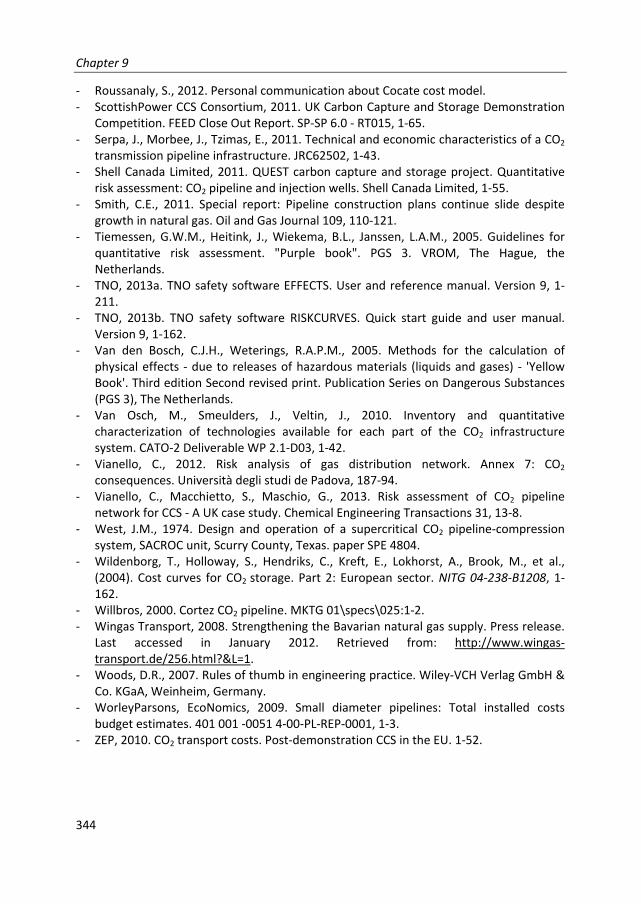
Chapter 9
344
‐ Roussanaly, S., 2012. Personal communication about Cocate cost model. ‐ ScottishPower CCS Consortium, 2011. UK Carbon Capture and Storage Demonstration
Competition. FEED Close Out Report. SP‐SP 6.0 ‐ RT015, 1‐65. ‐ Serpa, J., Morbee, J., Tzimas, E., 2011. Technical and economic characteristics of a CO2
transmission pipeline infrastructure. JRC62502, 1‐43. ‐ Shell Canada Limited, 2011. QUEST carbon capture and storage project. Quantitative
risk assessment: CO2 pipeline and injection wells. Shell Canada Limited, 1‐55. ‐ Smith, C.E., 2011. Special report: Pipeline construction plans continue slide despite
growth in natural gas. Oil and Gas Journal 109, 110‐121. ‐ Tiemessen, G.W.M., Heitink, J., Wiekema, B.L., Janssen, L.A.M., 2005. Guidelines for
quantitative risk assessment. "Purple book". PGS 3. VROM, The Hague, the Netherlands.
‐ TNO, 2013a. TNO safety software EFFECTS. User and reference manual. Version 9, 1‐211.
‐ TNO, 2013b. TNO safety software RISKCURVES. Quick start guide and user manual. Version 9, 1‐162.
‐ Van den Bosch, C.J.H., Weterings, R.A.P.M., 2005. Methods for the calculation of physical effects ‐ due to releases of hazardous materials (liquids and gases) ‐ 'Yellow Book'. Third edition Second revised print. Publication Series on Dangerous Substances (PGS 3), The Netherlands.
‐ Van Osch, M., Smeulders, J., Veltin, J., 2010. Inventory and quantitative characterization of technologies available for each part of the CO2 infrastructure system. CATO‐2 Deliverable WP 2.1‐D03, 1‐42.
‐ Vianello, C., 2012. Risk analysis of gas distribution network. Annex 7: CO2 consequences. Università degli studi de Padova, 187‐94.
‐ Vianello, C., Macchietto, S., Maschio, G., 2013. Risk assessment of CO2 pipeline network for CCS ‐ A UK case study. Chemical Engineering Transactions 31, 13‐8.
‐ West, J.M., 1974. Design and operation of a supercritical CO2 pipeline‐compression system, SACROC unit, Scurry County, Texas. paper SPE 4804.
‐ Wildenborg, T., Holloway, S., Hendriks, C., Kreft, E., Lokhorst, A., Brook, M., et al., (2004). Cost curves for CO2 storage. Part 2: European sector. NITG 04‐238‐B1208, 1‐162.
‐ Willbros, 2000. Cortez CO2 pipeline. MKTG 01\specs\025:1‐2. ‐ Wingas Transport, 2008. Strengthening the Bavarian natural gas supply. Press release.
Last accessed in January 2012. Retrieved from: http://www.wingas‐transport.de/256.html?&L=1.
‐ Woods, D.R., 2007. Rules of thumb in engineering practice. Wiley‐VCH Verlag GmbH & Co. KGaA, Weinheim, Germany.
‐ WorleyParsons, EcoNomics, 2009. Small diameter pipelines: Total installed costs budget estimates. 401 001 ‐0051 4‐00‐PL‐REP‐0001, 1‐3.
‐ ZEP, 2010. CO2 transport costs. Post‐demonstration CCS in the EU. 1‐52.
345
Dankwoord
4.5 jaar ben ik bezig geweest om onderzoek te doen naar de verschillende aspecten van CO2 infrastructuur ontwikkeling. Het resultaat van dit onderzoek ligt nu voor u. Maar dit boek was er niet gekomen, of had er op zijn minst heel anders uitgezien, zonder de hulp van anderen.
Als eerste wil ik graag mijn promotor André Faaij en copromotor Andrea Ramírez bedanken. Zonder André was ik waarschijnlijk nooit aan een promotie‐traject begonnen. Toen ik tijdens het afronden van mijn master thesis een keer informeerde naar de mogelijkheden van promoveren, reageerde hij zo enthousiast en vol vertrouwen dat ik niet langer twijfelde en de stap maakte. Ook tijdens mijn promotie‐traject had je een actieve rol, eerst in Utrecht en later vanuit Groningen. André, je hebt een gave om vrijwel in een oogopslag de zwakke punten uit een onderzoek te halen. Je suggesties om de verschillende artikelen na een hoger niveau te tillen waren altijd zeer waardevol.
Andrea, if I didn’t know where to go with my research anymore, you was always there to guide me into the right direction. You have a great eye for detail but also didn’t forget the great picture. Thanks for all you time and patient for answering my questions, discussions and providing comments on my (always relatively long) articles. Andrea and André, I would both like to thank you for the freedom you offered me for defining a large part of the scope of this thesis.
Verder wil ik graag Wim Guijt van Shell bedanken voor het beantwoorden van al mijn vragen over het ontwerpen, aanleggen, opereren en verwijderen van pijpleidingen. Voor mij was contact met iemand uit de industrie erg nuttig. De ‘reality‐check’ die je uitvoerde, heeft met name hoofdstuk 3 naar een hoger niveau getild. Onze verschillende gesprekken gaven me het gevoel dat mijn onderzoek niet alleen waardevol is voor wetenschappers, maar ook voor de industrie.
Hoofdstuk 4 was nooit tot stand gekomen zonder Ingrid Raben en Mark Spruijt van TNO. Ik vond het heel plezierig om met jullie samen te werken. Bedankt voor alle inzichten in de wereld van de veiligheid en risicoanalyse.
CATO‐2 heeft dit proefschrift financieel mogelijk gemaakt. Buiten dat heeft CATO‐2 verschillende interessante symposiums, leuke uitjes en gezellige PhD diners georganiseerd. Deze boden de mogelijkheid om echt deel uit te maken van de CATO‐2 gemeenschap en ook inzicht te krijgen in de andere delen van de CCS keten en aspecten van CCS implementatie. Dus CATO‐2, bedankt hiervoor.
Via de CATO‐2 gemeenschap, ben ik in contact gekomen met verschillende experts die hebben geholpen om meer inzicht te krijgen in de verschillende aspecten van CCS. Met het risico om iemand te vergeten, wil ik bij deze Chris Hendriks, Joris Koornneef (beide Ecofys), Jeremy Veltin, Stephan Belfroid, Philip Neele (alle drie TNO), Chantal Smulders (Shell), Wim Mallon (DNV‐GL) en Erwin Niessen (EBN) bedanken.

Dankwoord
346
Furthermore, I would like to thank all my colleagues for the nice talks during lunch, coffee breaks or just spontaneously in the hallways. A special thanks goes to all my colleagues who helped me with big and small questions related to CCS, software, modeling etc. Although we did not follow the same working hours, I couldn’t have a better roommate. Barbara, thanks that I always could share my frustration and good news with you. Bij deze wil ik ook Aisha, Siham, Petra en Fiona bedanken voor het uit handen nemen van de vele administratieve zaken die komen kijken bij een promotieonderzoek.
Af en toe moet je afstand nemen van je onderzoek om er daarna met een frisse blik naar te kijken. En wanneer gaat dat nu beter dan als met (schoon)familie en vrienden om je heen. Daarom wil ik bij deze al mijn (schoon)familie en vrienden bedanken voor alle gezellige etentjes, de goede gesprekken, de vrolijke borrels, de ontspannende weekendjes weg, de plezierige fiets‐ en wandeltochten, de geslaagde winkeluitjes en leerzame culturele uitjes van de afgelopen jaren.
Ik prijs mezelf gelukkig met ouders die mij de mogelijkheden en ruimte hebben gegeven om me te ontwikkelen en te doen wat ik graag wil. Mama, je hebt me geleerd om van het leven te genieten en op mijn gevoel te vertrouwen. Ik hoop dat je iets van jouw vlotte schrijfstijl terugvindt in dit boek. Papa, je hebt me geleerd om niet tevreden te zijn met een zes. De vaardigheid om overal lijstjes voor te maken, die ik van jou overgenomen heb, kwam zeer goed van pas de afgelopen 4.5 jaar.
Onno, meer nog dan ieder andere heb je de diepte‐ en hoogtepunten meegemaakt van mijn promotie‐traject. Bedankt voor je steun en grote vertrouwen op moeilijke momenten en je aanstekelijke enthousiasme zodra er iets te vieren is (ook al is het maar een eerste draftversie die opgestuurd is). Ik hoop nog heel veel hoogtepunten met jou te vieren!

347
Curriculum Vitae
Marlinde Knoope was born on 7th of November 1986 in Helvoirt, the Netherlands. She studied the bachelor Science and Innovation Management at Utrecht University. After her bachelor, she started with the master Energy Science at the same University. Her master thesis focused on assessing the learning potential, with a bottom‐up study as well as a top‐down approach, of gasification technologies for the production of power and Fischer‐Tropsch fuels with or without carbon capture and storage. After finishing her master, she started as a PhD student for the group Energy & Resources at the Copernicus institute of Utrecht University. The PhD project was part of the CATO‐2 program, the Dutch national research program on CO2 capture and storage. Her research investigated the cost, safety and uncertainties of CO2 infrastructure development system.
Peer reviewed articles and contributions:
‐ Knoope, M.M.J., Ramírez, A., Faaij, A.P.C., 2013. Future technological and economic performance of IGCC and FT production facilities with and without CO2 capture: Combining component based learning curve and bottom‐up analysis. International Journal of Greenhouse Gas Control 16, 287‐310.
‐ Meerman, J.C., Knoope, M.M.J., Ramirez, C.A., Turkenburg, W.C. & Faaij, A.P.C. (2013). Technical and economic prospects of coal‐ and biomass‐fired integrated gasification facilities equipped with CCS over time. International journal of greenhouse gas control, 16, 311‐323
‐ Knoope, M.M.J., Ramírez, A., Faaij, A.P.C., 2013. A state‐of‐the‐art review of techno‐economic models predicting the costs of CO2 pipeline transport. International Journal of Greenhouse Gas Control 16, 241‐270.
‐ Knoope, M.M.J., Guijt, W., Ramírez, A., Faaij, A.P.C., 2014. Improved cost models for optimizing CO2 pipeline configurations for point‐to‐point pipelines and simple networks. International Journal of Greenhouse Gas Control 22, 25‐46.
‐ Knoope, M.M.J., Raben, I., Spruijt, M., Ramírez, A., Faaij, A.P.C., 2014. The influence of risk mitigation measures on the risk contours, costs and routing of CO2 pipelines. International Journal of Greenhouse Gas Control 29, 104‐124.
‐ Knoope, M.M.J., Ramírez, A., Faaij, A.P.C., 2015. Investing in CO2 transport infrastructure under uncertainty: A comparison between ships and pipelines. International Journal of Greenhouse Gas Control 41, 174‐193.
(one more article is fortcoming, see chapter 6)

the Chairman of the SENSE board the SENSE Director of Education
Prof. dr. Huub Rijnaarts Dr. Ad van Dommelen
The SENSE Research School has been accredited by the Royal Netherlands Academy of Arts and Sciences (KNAW)
Netherlands Research School for the
Socio Economic and Natural Sciences of the Environment
D I P L O M AFor specialised PhD training
The Netherlands Research School for the
Socio Economic and Natural Sciences of the Environment
(SENSE) declares that
Marlinde Marissa Jasmijn Knoope
born on 7 November 1986 in Helvoirt, The Netherlands
has successfully fulfilled all requirements of the
Educational Programme of SENSE.
Utrecht, 4 September 2015

SENSE Coordinator PhD Education
Dr. ing. Monique Gulickx
The SENSE Research School declares that MsMarlinde Knoope has successfully fulfilled all
requirements of the Educational PhD Programme of SENSE with a work load of 45.5 EC,
including the following activities:
SENSE PhD Courses
o Basic Statistics (2011)
o Environmental Research in Context (2011)
o Research in Context Activity: Co organising the 7th Dutch CCS Symposium: Contributions of
SP2 (CO2 transport and chain integration) of CATO2 (2014)
Other PhD and Advanced MSc Courses
o Advanced GIS for geoscientists, Utrecht University (2012)
o Building models for GIS analysis using ArcGIS 10, ESRI online course (2013)
o Distance analysis using ArcGIS 10, ESRI online course (2013)
o Network analysis using ArcGIS 10, ESRI online course (2013)
o Python for everyone using ArcGIS 10.1, ESRI online course (2013)
o Transforming data using extract, transform and load processes, ESRI online course (2013)
o Using raster data for site selection for ArcGIS 10.1, ESRI online course (2013)
External training at a foreign research institute
o Summer School International Energy Agency Greenhouse Gas (IEA GHG), University of Illinois
(2011)
Management and Didactic Skills Training
o Supervising computer practicums of BSc course ‘Life Cycle Analysis’ and MSc course
‘Advanced Energy Analysis’ (2011 2013)
o Supervising the Consultancy Project of the MSc ‘Energy Science’ (2013)
o Supervising MSc student with thesis entitled ‘Assessing the role of ships in the development
of a CO2 transportation system for large scale storage in the North Sea’ (2014)
Oral Presentations
o The development of an economic optimization tool for CO2pipelines. 11th
International
Conference on Greenhouse Gas Technologies (GHGT 11), 18 22 November 2012, Kyoto,
Japan
o The influence of risk mitigation measures on the risk contours, costs and routing of CO2
pipelines. UKCCSRC CATO2 ECR Networking Meeting, 24 25 March 2014, York, United
Kingdom
o Pipeline safety vs. costs: How does it influence the CO2 transportation network? The 7th
Dutch
CCS symposium 19 20 June 2014, Amsterdam, The Netherlands