
Sedimentation on the Madeira Abyssal Plain: Eocene-Pleistocene history of turbidite infill
Upload
khangminh22Category
view
0download
0
Evaluation of uncertainties of thin oil turbidite reservoir using Experimental Design
Maura Serafina Matias Da Silva
Petroleum Engineering
Supervisor: Jon Kleppe, IPT
Department of Petroleum Engineering and Applied Geophysics
Submission date: August 2014
Norwegian University of Science and Technology

Maura Silva Page i
Abstract
This thesis concludes the degree of Master in Reservoir Engineering at the NTNU. The thesis
was conducted in collaboration with Maersk Oil Company in order to provide to the intern
valuable experience by using the reservoir simulator Eclipse and the software Petrel,
commonly applied in the oil industry. The report describes an application of different studies
performed in a real thin oil rim reservoir. It is oil with gas cap field located in the west of
Africa. The reservoir consists of various channels, which divide it into several compartments
with different heterogeneity and fluids oil contacts. In order to gain flexibility and ease testing
all studies were conducted in a sector model, consisting of the main compartment of the field.
The main goal of this thesis was to evaluate the uncertainties of the reservoir discovery using
experimental design. In this study the key uncertain parameters were relative permeability,
horizontal permeability and rock compressibility. A secondary objective was relate with
coning study, where the main objective was to estimate the critical oil production rate through
analytical correlations and numerical simulation, using available reservoir modeling tools.
The greatest challenge was obtaining a LGR resolution model with acceptable resolution and
CPU time, intending to improve simulation accuracy on the well bore region and to best
capture the cone. The process was time consuming and tedious but leaded to satisfactory
results. Finally, the report also describes three development schemes with water and gas
injection producing under critical oil rate, where the scenario with both gas and water
injection shows to be the most favorable scenario with 26% of oil recovered, and a coherent
solution to handle gas.
Maura Silva Page ii
Acknowledgement
First of all, I would like to thanks God, my great protector, for being the reason of existence
of all things, for all the blessings and always illuminate my way.
I also would like to thank my supervisor at Maersk Oil the reservoir engineer Sabrina Pereira.
Her professionalism and encouragement have been an inspiration every day in the office.
Thanks for all your guidance and motivational talks.
Thanks to the Maersk Oil Company for allow me to work in their office. The thesis would
never have been finished without this support.
I would like to express my gratitude to the people of the Exploration team of Maersk Oil
which has helped me with the thesis, especially the petroleum engineer Stig Adersen and the
reservoir engineer Bethany Rosenkrans. Both have been great consultants through interesting
and helpful conversations. Thank You.
Thanks to the engineers at Schlumberger, Eric Mahbou, for answering all my questions
regarding the software.
Sincere thanks go to my professional supervisor at the NTNU, Professor Jon Kleppe, for
motivational talks and guidance whenever needed.
Last but not least, my dearest greetings go to my lovely family: My mother Rita, for the love,
dedication, affection and unconditional support at all times of my life and for teaching me to
live with responsibility and above all with dignity. My dear sister Sonia and brother Edgar
for the affection. Thanks for all your support and patience throughout this period.
Thank You All!
Maura Silva Page iii
Table of Contents
Abstract ....................................................................................................................................... i
Acknowledgement ...................................................................................................................... ii
List of tables ............................................................................................................................. vii
List of equations ...................................................................................................................... viii
List of figures ............................................................................................................................ ix
Nomenclature ............................................................................................................................ xi
CHAPTER I – INTRODUCTION ........................................................................................... 13
1.1-Problem Description ....................................................................................................... 13
1.2 - Objective ...................................................................................................................... 14
CHAPTER II – LITERATURE REVIEW ............................................................................... 15
2.1- Coning concepts ............................................................................................................ 15
2.1.1 - Impact of coning .................................................................................................... 16
2.1.2 - Cause of coning ..................................................................................................... 17
2.1.3 - Handle the coning .................................................................................................. 17
2.2- Analytical correlations to predict coning ...................................................................... 18
2.2.1 - Giger & Karcher correlation .................................................................................. 18
2.2.2 - Joshi correlation ..................................................................................................... 19
2.2.3 – Work-Bench correlation ........................................................................................ 19
2.2.4 – Proxi model correlation ......................................................................................... 21
2.3 - Uncertainties ................................................................................................................. 21
2.3.1 - Management of reservoir uncertainties ................................................................. 23
2.3.2 - Assessment of reservoir uncertainties ................................................................... 23
2.3.2.1 – Experimental Design ...................................................................................... 23
2.3.2.1.1 - Full factorial designs in two levels ........................................................... 24
2.3.2.1.2 - Fractional factorial designs ...................................................................... 24
2.3.2.1.3 - Plackett-Burman designs .......................................................................... 24
2.3.2.1.4 - Central Composite Designs (CCD) .......................................................... 25
2.3.2.1.5 - D Optimal design ..................................................................................... 25
CHAPTER III - THE ALPHA FIELD ..................................................................................... 26
3.1 - Field description ........................................................................................................... 26
3.2 - Seismic acquisition ....................................................................................................... 27
3.3 - Evaluation of depositional environment and burial history ......................................... 28

Maura Silva Page iv
3.3.1 - Geological interpretation ....................................................................................... 29
3.3.2 - Sedimentological reservoir model ......................................................................... 30
3.4 - Strategy and developing plan ....................................................................................... 30
3.5 - Uncertainties in the Alpha reservoir data ..................................................................... 31
CHAPTER IV – THE SIMULATION MODEL...................................................................... 32
4.1 - Available data ............................................................................................................... 32
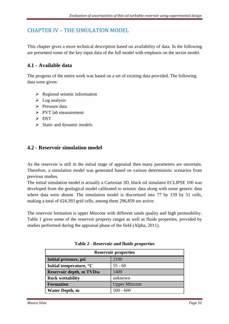
4.2 - Reservoir simulation model ......................................................................................... 32
4.2.1 – Sector model ......................................................................................................... 34
4.2.2- Model Input Data .................................................................................................... 34
4.2.2.1 - Fluid data ........................................................................................................ 35
4.2.2.2- Porosity ............................................................................................................ 36
4.2.2.3-Net to Gross ratio .............................................................................................. 37
CHAPTER V - DEVELOPING OF THE THESIS WORK .................................................... 38
5.1 – Impact of gridding (LGR)............................................................................................ 38
5.1.1-LGR on an irregular volume .................................................................................... 39
5.1.2 -Time steps ............................................................................................................... 39
5.1.3 - Convergence control .............................................................................................. 39
5.1.4 -The production well ................................................................................................ 39
5.1.5 - Scenario1 ............................................................................................................... 40
5.1.6 - Scenario 2 .............................................................................................................. 41
5.1.7 - Scenario 3 .............................................................................................................. 41
5.2 - Estimating critical oil rate on analytical study ............................................................. 42
5.2.1- Sensitivity analyses on estimated critical cone ....................................................... 42
5.3 -Estimating critical oil rate on numerical simulation study ............................................ 43
5.4 - Uncertainty parameters study ....................................................................................... 44
5.4.1 - Selecting the uncertainty parameters ..................................................................... 44
5.4.1.1- Relative permeability ....................................................................................... 44
5.4.1.2- Horizontal permeability ................................................................................... 45
5.4.1.3 - Vertical permeability ...................................................................................... 45
5.4.1.4 - Aquifer connectivity ....................................................................................... 45
5.4.1.5 - Rock Compressibility ...................................................................................... 46
5.4.1.6 - Well productivity index .................................................................................. 46
5.4.1.7 - Residual oil-to-water saturation ...................................................................... 46

Maura Silva Page v
5.4.2 - Generating the matrix design table using factorial fractional design method ....... 46
5.4.3 - Create the ED realizations depending on matrix design ........................................ 47
5.4.4 - Perform simulations for all realizations of the ED table ....................................... 48
5.4.5 - Import the results to an excel spreadsheet and generate the Pareto plot ............... 48
5.4.6 - Screening the key parameters from the Pareto plot ............................................... 49
5.5 - Impact of plateau length by producing above critical rate ........................................... 49
5.6 - Impact of surface constraints on production profiles ................................................... 49
5.7 - Improving oil recovery in the sector model ................................................................. 49
5.7.1- Gas injection scenario ............................................................................................. 50
5.7.2 - Water injection scenario ........................................................................................ 50
5.7.3 - Gas and water injection Scenario .......................................................................... 50
CHAPTER VI – RESULTS AND DISCUSSION ................................................................... 51
6.1 - LGR results .................................................................................................................. 51
6.2 - Analytical study results ................................................................................................ 54
6.2.1- Critical rate ............................................................................................................. 54
6.2.2 - Breakthrough time ................................................................................................. 56
6.2.3 - Sensitivity analyses ................................................................................................ 56
6.2.4 - Comparison between the methods ......................................................................... 58
6.3 - Results of the uncertainty parameters by using experimental design .......................... 58
6.3.1 - Pareto plot interpretation ....................................................................................... 58
6.3.2 - Uncertainty parameters discussion ............................................................................ 61
6.3.3 - Result of the three main cases generated from uncertainty study ......................... 62
6.3.4 - Results of impact on plateau length by producing above critical rate ................... 64
6.3.5 - Impact of surface constraints on profiles ............................................................... 66
6.4 - Results of IOR .............................................................................................................. 68
6.4.1 - Gas injection scenario ............................................................................................ 68
6.4.2 - Results of Water injection scenario ....................................................................... 71
6.4.4 - Results of both gas & water injection scenario ..................................................... 74
6.4.5 - Comparison of three case scenarios results ........................................................... 76
6.4.6 - Analog recovery factors ......................................................................................... 78
CHAPTER VII – CONCLUSION ........................................................................................... 79
RECOMMENDATIONS FOR FURTHER WORK ................................................................ 80
REFERENCE ........................................................................................................................... 81

Maura Silva Page vi
APPENDICES .......................................................................................................................... 84
Maura Silva Page vii
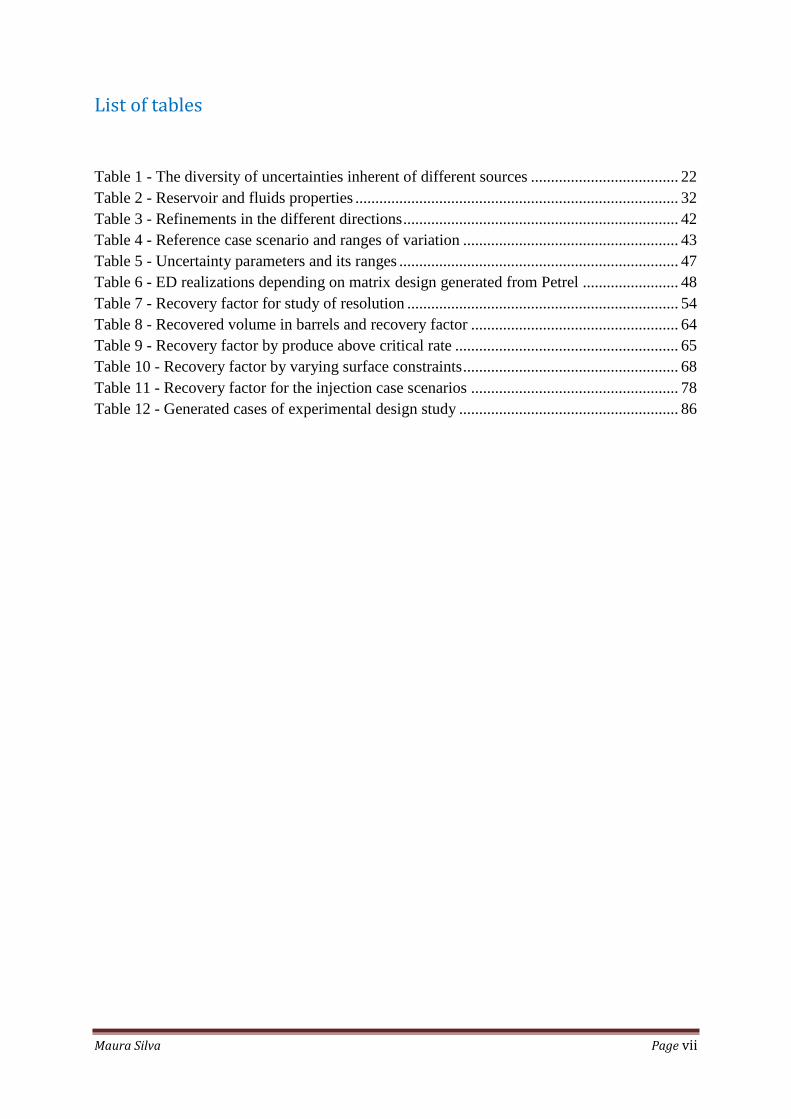
List of tables
Table 1 - The diversity of uncertainties inherent of different sources ..................................... 22
Table 2 - Reservoir and fluids properties ................................................................................. 32
Table 3 - Refinements in the different directions ..................................................................... 42
Table 4 - Reference case scenario and ranges of variation ...................................................... 43
Table 5 - Uncertainty parameters and its ranges ...................................................................... 47
Table 6 - ED realizations depending on matrix design generated from Petrel ........................ 48
Table 7 - Recovery factor for study of resolution .................................................................... 54
Table 8 - Recovered volume in barrels and recovery factor .................................................... 64
Table 9 - Recovery factor by produce above critical rate ........................................................ 65
Table 10 - Recovery factor by varying surface constraints ...................................................... 68
Table 11 - Recovery factor for the injection case scenarios .................................................... 78
Table 12 - Generated cases of experimental design study ....................................................... 86
Maura Silva Page viii
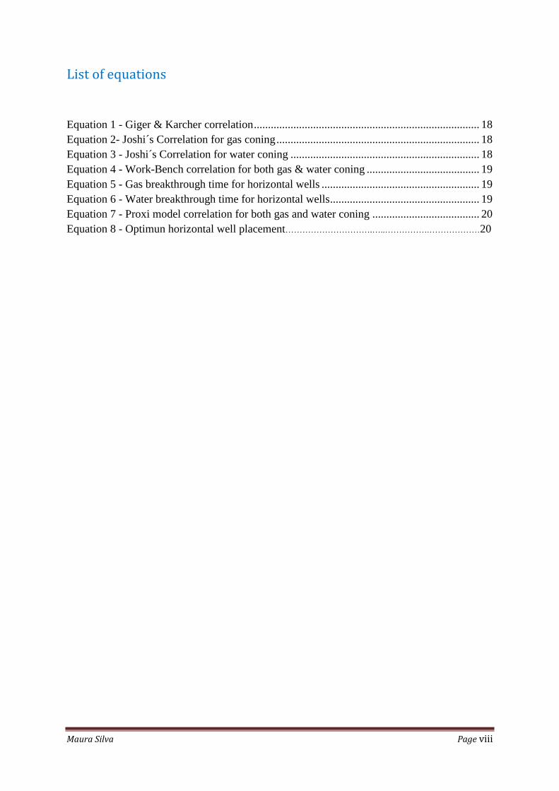
List of equations
Equation 1 - Giger & Karcher correlation ................................................................................ 18
Equation 2- Joshi´s Correlation for gas coning ........................................................................ 18
Equation 3 - Joshi´s Correlation for water coning ................................................................... 18
Equation 4 - Work-Bench correlation for both gas & water coning ........................................ 19
Equation 5 - Gas breakthrough time for horizontal wells ........................................................ 19
Equation 6 - Water breakthrough time for horizontal wells ..................................................... 19
Equation 7 - Proxi model correlation for both gas and water coning ...................................... 20
Equation 8 - Optimun horizontal well placement………………………….…..…………….………………20
Maura Silva Page ix
List of figures
Figure 1 - Double coning in a vertical well. ............................................................................. 15
Figure 2 - Coning in a horizontal well ..................................................................................... 16
Figure 3 - Structural cross sections through Petrel model ....................................................... 26
Figure 4 - Petrel illustration of full field model ....................................................................... 27
Figure 5 - Post-Salt Stratigraphy and Structural Events of the Alpha field ............................. 28
Figure 6 - Alpha field showing the area of Sector Model in blue dark .................................... 33
Figure 7 - Liquid formation volume factor vs. pressure captured from petrel ......................... 35
Figure 8 - Oil viscosity vs. pressure captured from petrel ....................................................... 35
Figure 9 - Gas formation volume factor vs. pressure captured from petrel ............................. 36
Figure 10 - Gas viscosity vs. pressure captured from petrel .................................................... 36
Figure 11 - Porosity distribution in the model ......................................................................... 37
Figure 12 - Net-to-Gross ratio distribution in the model ......................................................... 37
Figure 13 - Schematic overview of the main scenarios performed in this thesis ..................... 38
Figure 14 - Production well trajectory ..................................................................................... 40
Figure 15 - Illustration of LGR 3x3x3 resolutions inside the polygon used in the model ....... 40
Figure 16 - Illustration of LGR 5x5x5 resolutions inside the polygon used in the model ....... 41
Figure 17 - Illustration of LGR 7x7x7 resolutions inside the polygon used in the model ....... 41
Figure 18 - Relative Permeability Curves (water-oil system) .................................................. 45
Figure 19 - Matrix design generated from Petrel ..................................................................... 47
Figure 20 - Sector model showing the set of injection wells ................................................... 50
Figure 21 - cross sectional view of the well with different resolutions ................................... 51
Figure 22 - CPU time for the different resolutions .................................................................. 51
Figure 23 - Oil production rate for different resolutions .......................................................... 52
Figure 24 - Field water cut for different resolutions ................................................................ 52
Figure 25 - Gas oil ratio for different resolution ...................................................................... 53
Figure 26 - field oil production total at different resolution .................................................... 53
Figure 27- Cross section view of the coning progress over the time ....................................... 54
Figure 28 - Estimated critical oil rate by different correlations ............................................... 55
Figure 29 - Breakthrough time ................................................................................................. 56
Figure 30 - Critical oil rate as a function of horizontal permeability ....................................... 57
Figure 31- Critical oil rates calculated as a function of the well length ................................... 57
Figure 32 - Critical oil rate as a function of oil viscosity ......................................................... 58
Figure 33 - Impact of uncertainties on oil recovery on Pareto plot .......................................... 59
Figure 34 - Oil production rate vs. time of the experimental design study .............................. 60
Figure 35 - Gas oil ratio vs. time of the experimental design study ........................................ 60
Figure 36 - Oil production cumulative vs. time of the experimental design study .................. 61
Figure 37 - Gas oil rate vs. time for the three main case of experimental design .................... 62
Figure 38 - Water cut vs. time for the three main case of experimental design ....................... 63
Figure 39 - Field oil production total vs. time for the three main case of experimental design
.................................................................................................................................................. 63

Maura Silva Page x
Figure 40 - Field oil production rate vs. time for the three main case of experimental design 64
Figure 41 - Field oil production total vs. time for the three main case of experimental design
.................................................................................................................................................. 65
Figure 42 - Gas oil ratio vs. time for the test of fluid constraints ............................................ 66
Figure 43 - Field Water cut vs. time for the test of fluid constraints ....................................... 66
Figure 44 - Oil production rate vs. time for the test of fluid constraints .................................. 67
Figure 45 - Oil production Cumulative vs. time for study of the test constraints .................... 67
Figure 46 - field oil production rate vs. time for gas injection scenario .................................. 68
Figure 47 - Figure field gas oil ratio vs. time for gas injection scenario ................................. 69
Figure 48 - Figure field water cut vs. time for gas injection scenario ...................................... 69
Figure 49 - Field pressure vs. time for gas injection scenario .................................................. 70
Figure 50 - Reservoir volume production and injection rate vs. time for gas injection scenario
.................................................................................................................................................. 70
Figure 51 - Field oil production total vs. time for gas injection scenario ................................ 71
Figure 52 - Field gas oil ratio vs. time for water injection scenario ........................................ 71
Figure 53 - Reservoir volume production and injection rate vs. time for water injection
scenario ..................................................................................................................................... 73
Figure 54 - Field oil production total vs. time for water injection scenario ............................. 73
Figure 55 - Field gas oil ratio vs. time for gas & water injection scenario .............................. 74
Figure 56 - Reservoir volume production and injection rate vs. time for gas & water injection
scenario ..................................................................................................................................... 74
Figure 57 - Field pressure vs. time for gas & water injection scenario .................................... 75
Figure 58 - field water cut vs. time for gas & water injection scenario ................................... 75
Figure 59 - field gas oil ratio for injection cases ...................................................................... 76
Figure 60 - Field water cut field for injection cases ................................................................. 76
Figure 61 - Field pressure vs. time for injection cases ............................................................. 77
Figure 62 - field oil production total vs. time for injection cases ............................................ 77
Figure 63 - Analog Recovery Factors for Oil Rim with Gas Cap, Offshore Fields outside
Africa ........................................................................................................................................ 78
Figure 64 - critical oil correlation on VBA .............................................................................. 84
Figure 65 - Defining variables to generate the design matrix on Petrel ................................... 85
Figure 66 - Selecting method and and generating matrix design ............................................. 85
Figure 67 - Program sequence to generate Pareto plot (a) ....................................................... 87
Figure 68 - Program sequence to generate Pareto plot (b) ....................................................... 87
Figure 6969 - Gas production cumulative vs. time of the ED cases ........................................ 88
Figure 70 - Water production rate vs. time of the ED cases .................................................... 89
Figure 71 - Water cut vs. time of the ED cases ........................................................................ 90
Figure 72 - Pressure vs. time of the ED cases .......................................................................... 90
Figure 73 - CPU time vs. time of the ED cases........................................................................ 91
Figure 74 - Gas production cumulative and oil production rate vs. time of the three main ED
cases ......................................................................................................................................... 91
Figure 75 - gas and oil production rate vs. time of the three main ED cases ........................... 92
Figure 76 - Oil production cumulative and oil production rate of the three scenarios of the
IOR study ................................................................................................................................. 92
Maura Silva Page xi
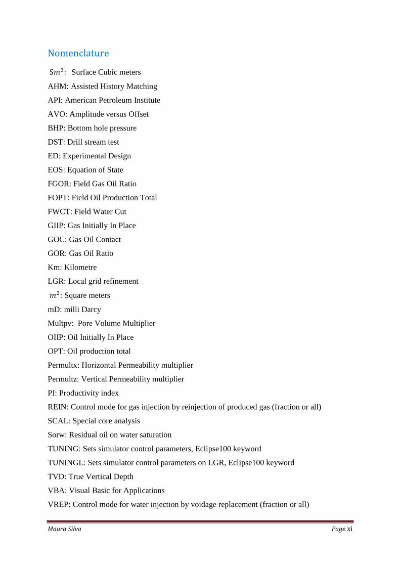
Nomenclature
Surface Cubic meters
AHM: Assisted History Matching
API: American Petroleum Institute
AVO: Amplitude versus Offset
BHP: Bottom hole pressure
DST: Drill stream test
ED: Experimental Design
EOS: Equation of State
FGOR: Field Gas Oil Ratio
FOPT: Field Oil Production Total
FWCT: Field Water Cut
GIIP: Gas Initially In Place
GOC: Gas Oil Contact
GOR: Gas Oil Ratio
Km: Kilometre
LGR: Local grid refinement
: Square meters
mD: milli Darcy
Multpv: Pore Volume Multiplier
OIIP: Oil Initially In Place
OPT: Oil production total
Permultx: Horizontal Permeability multiplier
Permultz: Vertical Permeability multiplier
PI: Productivity index
REIN: Control mode for gas injection by reinjection of produced gas (fraction or all)
SCAL: Special core analysis
Sorw: Residual oil on water saturation
TUNING: Sets simulator control parameters, Eclipse100 keyword
TUNINGL: Sets simulator control parameters on LGR, Eclipse100 keyword
TVD: True Vertical Depth
VBA: Visual Basic for Applications
VREP: Control mode for water injection by voidage replacement (fraction or all)

Maura Silva Page xii
WCT: Water cut
WGPR: Well Gas Production Rate
WOC: Water Oil Contact
WOPT: Well Oil Production Total
WTHP: Well tubing head pressure
Ye: Half Drainage area

Evaluation of uncertainties of thin oil turbidite reservoir using experimental design
Maura Silva Page 13
CHAPTER I – INTRODUCTION
1.1-Problem Description
A strategic development project of an oil field aims as a general rule to accelerate the
hydrocarbon production and maximize the recovery at a lowest cost. For thin oil rim reservoir
with a large gas cap on top and a strong aquifer on bottom, achieving such goal can be very
challenging since recovery of oil shall be maximized. This trend has initiated increasing
efforts to improve advanced technologies in order to make less expensive and more profitable
the exploitation of thin oil reservoirs. Since, some of them were abandoned in the past, being
characterized as non-commercial reserves due the inexistence of adequate technologies. In
this context today are notable few reserves around the world, which initially thought to not
have any commercial value at first evaluation.
One of the most challenging tasks that such reservoirs present is related to its complicated
production mechanism. Due to the very thin oil zone and pressure drawdown around the well
bore, during the production process fluid interfaces are not stable during the production
process thereby a phenomenon referred as coning or cresting depending on the well
completion (Khalili, 2005). While coning is related with the fluid motion towards the
perforation of a vertical well, cresting happens when comes to horizontal wells. Therefore,
many authors address the problem only as coning. The term cone is nothing more than the
tendency of gas and water to push oil towards the well in a cone shaped contour. It occurs
when viscous forces exceed gravity forces near the well bore of a producing well. As soon as
the cone breaks through the well, gas or water production increases substantially leading a
drastic drop in reservoir pressure and consequently affecting the oil production (Kazeem et al,
2010). Surface Constraints are a critical element in the development of oil rim.
In fact, after a certain period of production a reservoir often presents high production level of
gas or water, when its respective lines of contact with oil reach the perforation, but this should
not be confused with coning phenomena; where the unwanted fluids due the tortuosity of the
reservoir find channels to flow and easily reach the perforations. It is important to highlight
that cone is more likely to occur when a well is producing at high rates. Coning problem in
thin oil reservoirs can occurs even sooner than in conventional reservoirs, affecting seriously
the overall recovery efficiency, leaving significant amount of oil behind and consequently
increase cost of production operation (Olamigoke et al, 2009).
As this thesis work is focused on a specific thin oil reservoir, which is considered a three fluid
phase system the Muskat and Wyckoff method was discarded in this study. In order to portray
a similar panoramic of the reservoir under study an especial attention will be given to Work-
Bench and Proxi model correlations; which are a three phase, black oil model and suitable for
coning.
Evaluation of uncertainties of thin oil turbidite reservoir using experimental design
Maura Silva Page 14
In general this thesis work addresses the double coning problem of thin oil rim reservoirs with
a horizontal well. In order to provide some understanding the mathematical and physical
principles behind this process are briefly reviewed.
For the propose of evaluate uncertainty and impact of the various parameters a sensitivity
study will be performed, where a number of possible scenarios characterized by different
combination of petrophysical and fluid properties was conducted and the obtained results will
be displayed and discussed with respect to their simplifying assumptions.
1.2 - Objective
The main objective is to evaluate uncertainty on recovery factor of an oil-rim reservoir using
reservoir simulation and Experimental Design.
Others objectives will be also considered such us:
Understanding the physics behind the cone phenomena.
Providing an overview of the most relevant parameters that affect water/gas coning by
using analytical calculations.
Improving simulation accuracy on the well bore region in order to best capture the
cone by using LGR.
Accessing uncertainties parameters that most affect the overall oil recovery and how
to deal with by using experimental design tool.
Investigating a development scheme with water and/or gas injection.

Evaluation of uncertainties of thin oil turbidite reservoir using experimental design
Maura Silva Page 15
CHAPTER II – LITERATURE REVIEW
Attenuate gas or water coning problems during oil production in conventional oil reservoirs is
a challenge task but deal with such problem in a thin oil rim reservoir make the process even
more complex. Therefore, this chapter outlines concepts behind the coning phenomena and
ways to handle it when refers to thin oil accumulations. A few models that can be used to
predict critical rate will be mentioned. Procedures used in analytical as well as numerical
simulation will be pointed, and its utilities will be discussed.
Then, chapter will give a review of the uncertainties inherent in reservoir with associated
impact, and a brief overview of experimental design methodologies as current practice widely
used in the industry in quantifying and assessing uncertainties.
2.1- Coning concepts
The term coning is used to describe the mechanism of unwanted fluids trend to flow into the
perforation of a production well in a coning shape, due the viscous and gravitational forces in
a reservoir. In a system with distinct fluids phase two forces act upon the interface between
the oil and the unwanted fluid: viscous forces that result as consequence of fluid production
and gravitational forces that arise from the density difference between the two fluids and
which tend to counterbalance the viscous forces. If the viscous forces exceed the gravitational
forces, then a cone is formed and grows towards the wellbore until the viscous forces at some
elevation. If such balance is never achieved, the cone continues to grow and the unwanted
fluid breaks into the wellbore (Ozkan et al, 1990). Coning occurs when viscous forces
dominate.
The term coning is used because, in a vertical well, the shape of the interface when a well is
producing the second fluid resembles an upright or inverted cone. The figure 1 shows a
double coning in a vertical well.
Figure 1 - Double coning in a vertical well
.
In fact, there are three essential forces playing key role in the coning mechanism. They are
capillary, gravity and viscous forces. For simplicity, the process is assumed to be dominated
by viscous forces and capillary forces are therefore neglected. Before production, the gravity
force, which is a consequence of the density difference between the fluids, is dominant. Once
Evaluation of uncertainties of thin oil turbidite reservoir using experimental design
Maura Silva Page 16
a well is allowed to produce oil, the viscous forces which result from pressure drawdown
increase. In order to counterbalance the system, water oil contact (WOC) deforms and moves
up until viscous force is balanced by the gravitational force at a certain elevation, that is, at a
certain flow rate, there is a point at which a balance can be achieved between the viscous
force and the gravity force. If such a balance is never achieved the cone will be dragged up
until it will break into the wellbore (Veskimägi, 2013). The shape and the nature of the cone
depend on several factors such as production rate, mobility ratio, horizontal and vertical
permeability, well penetration and viscous forces.
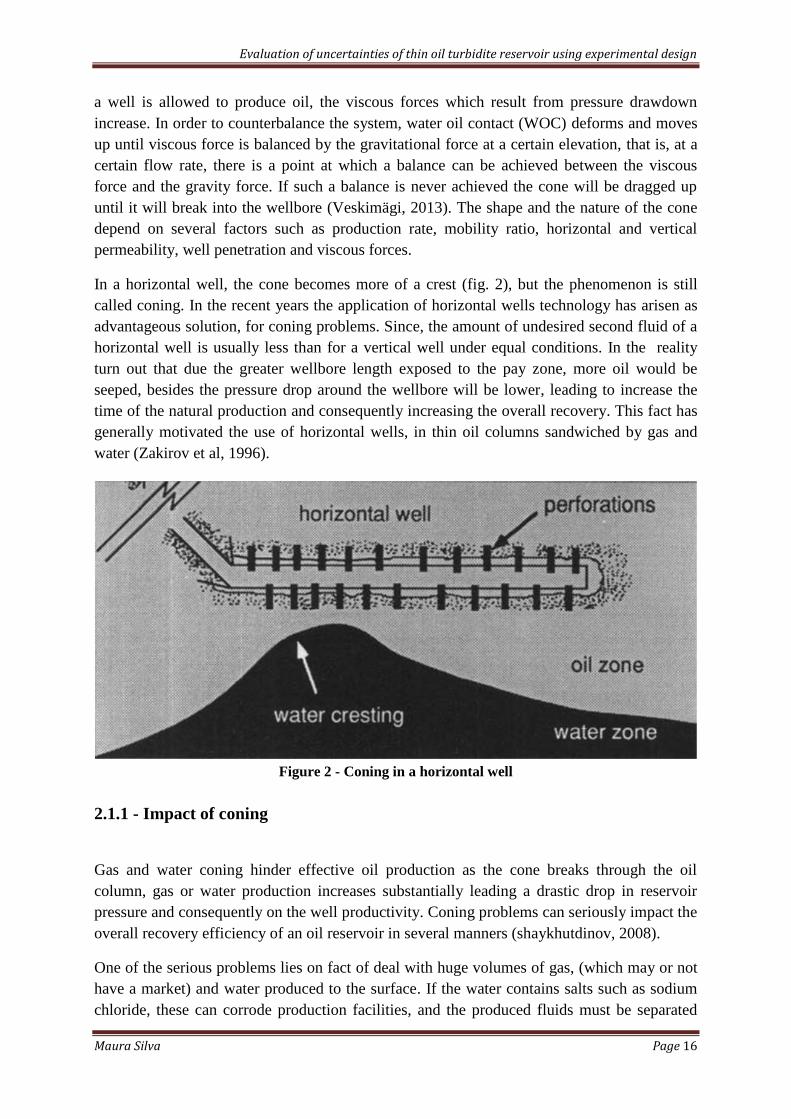
In a horizontal well, the cone becomes more of a crest (fig. 2), but the phenomenon is still
called coning. In the recent years the application of horizontal wells technology has arisen as
advantageous solution, for coning problems. Since, the amount of undesired second fluid of a
horizontal well is usually less than for a vertical well under equal conditions. In the reality
turn out that due the greater wellbore length exposed to the pay zone, more oil would be
seeped, besides the pressure drop around the wellbore will be lower, leading to increase the
time of the natural production and consequently increasing the overall recovery. This fact has
generally motivated the use of horizontal wells, in thin oil columns sandwiched by gas and
water (Zakirov et al, 1996).
Figure 2 - Coning in a horizontal well
2.1.1 - Impact of coning
Gas and water coning hinder effective oil production as the cone breaks through the oil
column, gas or water production increases substantially leading a drastic drop in reservoir
pressure and consequently on the well productivity. Coning problems can seriously impact the
overall recovery efficiency of an oil reservoir in several manners (shaykhutdinov, 2008).
One of the serious problems lies on fact of deal with huge volumes of gas, (which may or not
have a market) and water produced to the surface. If the water contains salts such as sodium
chloride, these can corrode production facilities, and the produced fluids must be separated
Evaluation of uncertainties of thin oil turbidite reservoir using experimental design
Maura Silva Page 17
before transporting to the refinery (Onwukwe et al, 2012). Besides, in terms of cost it implies
increase operating expenses with some extra surface facilities to separate the produced water
from oil and all lead to reduced revenue.
2.1.2 - Cause of coning
Silva et all (2010) claim that the increasing production of unwanted fluids coming from
coning problems is generally associated with high producing rates.
The rate above which the pressure gradients in the system cause the cone to break into the
well is defined as the critical production rate in the literature. Even when all the assumptions
of the critical rate concept hold, technical and economic necessities may enforce production
rates above the critical rate (Makinde et al, 2011). It is therefore important to predict the
evolution of the cone and the time breakthrough so that future completion and production
schemes can be envisaged.
2.1.3 - Handle the coning
Unfortunately, coning formation cannot be avoided in reservoirs with a thin oil-bearing layer,
sandwiched between gas cap and bottom or edge water, and in such cases both gas and water
coning can occur simultaneously. In consequence, the exploitation of these reservoirs poses a
challenge for reservoir development, as early gas and water coning severely hinder maximum
oil recovery. Alleviating these challenges by reservoir management involves knowing where
the fluid contacts are, optimization of well placement and predict a critical rate that will
generate a stable and controlled cone below the perforation.
In general operating a production well at critical rate is usually appointed as the most efficient
way to avoid anticipated coning problems. Hamed (2000), defines the critical production rate
as the rate above which the flowing pressure gradient at the well causes gas or water to cone
breaking into the well. In other words it is the maximum rate of oil production without
concurrent production of the displacing phase by coning. However, due to economic
necessities, oil companies often produce at a rate higher than critical coning rate. This causes
water or gas coning or simultaneous coning of water and gas. Therefore, if the oil flow rate of
a well exceeds the critical coning rate calculated for this well the cone becomes unstable and
will break into the wellbore after a certain time. At this stage, the well performance becomes
important, it merits careful attention and having knowledge of breakthrough time may help to
improve well management and extend well life without production of water or free gas
(Recham, 2001).
In this context, apart from predict the critical rate, prediction of the breakthrough time is also
crucial for oil wells subject to gas/water coning problems as well as to evaluate the well
performance after breakthrough. A survey of the literatures shows that several researches have
been carrying out around the subject. This ranges from experimental coning studies to
analytical and numerical simulation studies aimed at understanding and predicting coning;

Evaluation of uncertainties of thin oil turbidite reservoir using experimental design
Maura Silva Page 18
which usually imply estimate critical rate, time breakthrough and time after breakthrough in
vertical and horizontal wells. However, there is no guarantee of how great the analytical
methods are in terms of accuracy (when using to predict coning), because they all contain
significant simplifying assumptions (Yang, 1991).
As analytical methods often fail to reliably describe real systems because of their inherent
limitations, numerical models are also used in addition to predict cone, since they represent in
fact the only viable option for describing any type of fluid flow problem in complex reservoirs
problems. Accordingly, the prediction analytical methods are best used for quick
approximations, screening, and comparison of alternatives, and will require further reservoir
simulations, based on accurate reservoir characterization (Verga et al, 2007).
Moreover cone can also be stimulated or attenuated in numerical models by a setting of
constraints on the production well. The well is assumed to produce under specified conditions,
where the target of gas and liquid allowed to be produced can be specified, in order to
maximize oil production, while honor the sets well constraints. In other words while
implementing surface constraints it will limit coning effects by prevent high production of gas
and water.
2.2- Analytical correlations to predict coning
Most of the published works that address conning problem have developed correlations
assuming that only oil and gas or oil and water are present at reservoir conditions (two phase
systems). However, when refers to reservoirs with thin oil zones sandwiched between gas cap
and bottom water this scenario changes. Since, it will deal with three phase fluid system and
for these cases is believed that those correlations will not work out the same way. It would
probably require adjustments in order to preserve the real reservoir conditions. Based on the
most used analytical methods to predict the critical rate for horizontal wells, in the following
sections are presented four correlations, where two of them were developed to describe the
cone behave of a two phase system and the other two were specially developed to portray the
cone behave in thin oil reservoirs. The idea was to evaluate whether those developed for two
phase system would provide similar results as the one destined to three phase systems.
2.2.1 - Giger & Karcher correlation
Giger (1989) presented an analytical 2-D mathematical model of water cresting before
breakthrough for horizontal wells. He used the free surface boundary condition and assumed
that the free surface is at a large distance from the well, as the oil height in the model may be
difficult to choose. The author suggested that these solutions should not be used for small
values of the drainage radius, since he modified the mathematical solution based on the
comparison with experimental data (Verga et al, 2007).

Evaluation of uncertainties of thin oil turbidite reservoir using experimental design
Maura Silva Page 19
Equation 1 shows the respective developed correlation to estimate the critical rate in two
phase system. The density difference term ( ) to be used in the equation is ( ) for a
single gas cone and ( ) for a single water cone.
[
] *
+ * (
)
+
2.2.2 - Joshi correlation
Joshi (1988, 1991) studied the productivity of slanted and horizontal wells using the potential
fluid theory. The mathematical solution of his theory was simplified by subdividing the three-
dimensional fluid flow problem into two bi-dimensional problems, namely oil flow into a
horizontal well in a horizontal plane and in a vertical plane. He also compared horizontal
wells to vertical wells in terms of critical rate and gas and water coning occurrence, providing
an equation for the calculation of critical rates for gas coning (Eq. 2) and water coning (Eq. 3)
systems (Gawish, 2007).
[
]
[
]
Where:
[ ]
[ √ [ ] ][ ]
√
[ √ ]
2.2.3 – Work-Bench correlation
The Work-Bench is a standard numerical model, three phase, and black oil model with finite
difference formulation with simultaneous and direct solution and therefore suitable for coning
studies. Its validity has been extensively tested over the last years (Recham, 2001). This
approach was specially developed to deal with three phase fluid system and aim to predict,
optimum oil rate, water breakthrough time and gas breakthrough time for both vertical and

Evaluation of uncertainties of thin oil turbidite reservoir using experimental design
Maura Silva Page 20
horizontal wells. The following equations are the correlations to estimate the critical rate and
the breakthrough time for both gas and water in horizontal wells.
(
)
(
)
(
)
(
)
Where:
√
Gas breakthrough time for horizontal wells:
(
)
(
)
(
)
(
)
(
)
[ (
)
]
[ (
)
]
(
)
Where:
( )√
Water breakthrough time for horizontal wells:
(
)
(
)
(
)
(
)
(
)
(
)
Where:
√
Evaluation of uncertainties of thin oil turbidite reservoir using experimental design
Maura Silva Page 21
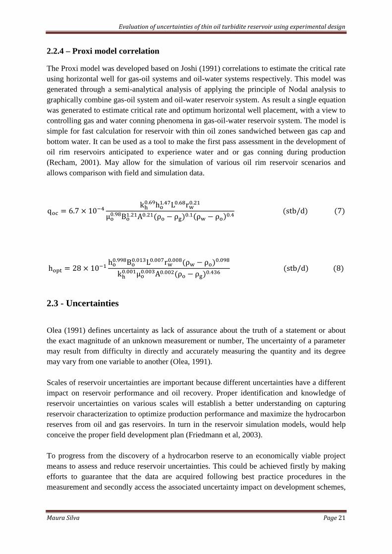
2.2.4 – Proxi model correlation
The Proxi model was developed based on Joshi (1991) correlations to estimate the critical rate
using horizontal well for gas-oil systems and oil-water systems respectively. This model was
generated through a semi-analytical analysis of applying the principle of Nodal analysis to
graphically combine gas-oil system and oil-water reservoir system. As result a single equation
was generated to estimate critical rate and optimum horizontal well placement, with a view to
controlling gas and water conning phenomena in gas-oil-water reservoir system. The model is
simple for fast calculation for reservoir with thin oil zones sandwiched between gas cap and
bottom water. It can be used as a tool to make the first pass assessment in the development of
oil rim reservoirs anticipated to experience water and or gas conning during production
(Recham, 2001). May allow for the simulation of various oil rim reservoir scenarios and
allows comparison with field and simulation data.
2.3 - Uncertainties
Olea (1991) defines uncertainty as lack of assurance about the truth of a statement or about
the exact magnitude of an unknown measurement or number, The uncertainty of a parameter
may result from difficulty in directly and accurately measuring the quantity and its degree
may vary from one variable to another (Olea, 1991).
Scales of reservoir uncertainties are important because different uncertainties have a different
impact on reservoir performance and oil recovery. Proper identification and knowledge of
reservoir uncertainties on various scales will establish a better understanding on capturing
reservoir characterization to optimize production performance and maximize the hydrocarbon
reserves from oil and gas reservoirs. In turn in the reservoir simulation models, would help
conceive the proper field development plan (Friedmann et al, 2003).
To progress from the discovery of a hydrocarbon reserve to an economically viable project
means to assess and reduce reservoir uncertainties. This could be achieved firstly by making
efforts to guarantee that the data are acquired following best practice procedures in the
measurement and secondly access the associated uncertainty impact on development schemes,

Evaluation of uncertainties of thin oil turbidite reservoir using experimental design
Maura Silva Page 22
improve the reservoirs appraisals, and manage their developments more efficiently (Riegert et
al, 2007).
Accordingly, a large number of uncertainties can be identified and classified into different
groups. Table 1 shows the diversity of uncertainties inherent of different sources. These
sources combine several types of data, including geological, seismic, petrophysical, and well
data (Walstrom et al, 1967).
Table 1 - The diversity of uncertainties inherent of different sources
Type of
uncertainty Difficult accuracy Impact
Uncertainty in
geophysical data
Uncertainties and errors in picking
Affects reservoir
envelope and its
fault system
diference between several interpretations
Uncertainties and errors in depth conversion
Uncertainties in the seismic
Uncertainties in pre-processing and migration
Uncertainties in the top map reservoir
Uncertainty
Geological data
Uncertainties in gross rock volume
Uncertainties in the extension and orientation of
sedimentary bodies Results in
uncertainties on
reservoir
sedimentary and
petrophysics-that
influence the
hydrocarbons
volume in place and
the dynamic of
fluids
Uncertainties in the distribution, shape and
limits of reservoir rock types
Uncertainties in the porosity values and their
distribution
Uncertainties in horizontal permeability values
and their distribution
Uncertainties in the layers Net to gross ratio
Uncertainties in the reservoir fluids contacts
Uncertainty in
dynamic reservoir
data
Horizontal permeability
Have impact on the
determination of
reserves and
production profiles
permeability anisotropy
Vertical to horizontal permeability
relative permeability parameters
capillary pressure ccurves
Aquifer behaviour
Fault sealing transmissibility
Extension of horizontal and vertical barriers
well productivity index and infectivity index
well skin
Uncertainty of
reservoir fluids
data
Lack of representative reservoir fluid samples
impact the on the
optimization of the
processing
capacities of oil and
gas
Uncertainty in reservoir samples from different
reservoir zones
Uncertainty in the compositional analyses
Uncertainty in the PVT laboratory
measurements
Uncertainty in the reservoir interfacial tension
Evaluation of uncertainties of thin oil turbidite reservoir using experimental design
Maura Silva Page 23
2.3.1 - Management of reservoir uncertainties
In undeveloped reservoirs, there are always many uncertain parameters affecting management
and decision making in a development plan stage. The diversity of inherent uncertainties and
how they impact the predicted hydrocarbon accumulation and recovery in the reservoir
require carefully analyze and therefore, the proper and unbiased decisions for oil reservoir
development can be made.
Management of uncertainty, would require identify uncertainties, both of the reservoir’s static
geometry and of its dynamic behavior (Friedmann et al 2003). For this purpose statistic
approaches provide a means of estimating the probability of outcomes from the uncertainty
variables. A rigorous approach of all possible realizations would imply a very large number of
simulations run making the process complicated and time consuming. Therefore, encouraging
solutions can be achieved.
2.3.2 - Assessment of reservoir uncertainties
To access the effect of uncertainties a systematic and efficient approach based in statistics
methods called Experimental Design has been widely used; where a set of reservoirs
parameters are chosen from their specific ranges in such a manner that the uncertainty in the
system is captured with the least number of simulations runs. Experimental Designs is often
used in diverse workflows to quantify uncertainties and to investigate the propagation of
parameter uncertainties by using Monte Carlo and Proxy sampling techniques (Begg 2001).
In other words it consists in performing an uncertainty workflow to generate many
realizations of the model. Each of the uncertainties is allowed to vary within prescribed
ranges. It is a useful tool firstly for saving simulation time and secondly for assessing a large
number of uncertainty parameters and selecting the ones that have more impact.
2.3.2.1 – Experimental Design
Experimental design is a structured methodology used to determine the relationship between
the different factors affecting a process and the output of that process. The methodology
offers not only an efficient way of assessing uncertainties by providing inference with
minimum number of simulations, but also can identify the key parameters governing
uncertainty in economic and production forecast (Yeten et al, 2005). Attempts to generate a
mathematical model that describes the process there are many experimental design methods,
the selection of which often depends on the objective of the exercise (Itotoi et al, 2010). The
following sections will focus on different techniques of experimental design based on
probabilistic method process with emphasis to fractional factorial design which is the method
used in this study.

Evaluation of uncertainties of thin oil turbidite reservoir using experimental design
Maura Silva Page 24
2.3.2.1.1 - Full factorial designs in two levels
A design in which every setting of every factor appears with every setting of very other factor
is a full factorial design. A common experimental design is one with all input factors set at
two levels each. These levels are called high and low or +1 and -1, respectively. A design with
all possible high/low combinations of all the input factors is called a full factorial design in
two levels. If there are k factors, each at two levels, a full factorial design has runs (Itotoi
et al, 2010).
2.3.2.1.2 - Fractional factorial designs
Fractional factorial design is defined as a factorial experiment in which only an adequately
chosen fraction of the treatment combinations required for the complete factorial experiment
is selected to be run (ASQC, 1983).
The design is mainly used for screening objective where the primary purpose of the
experiment is to select or screen out the few important main effects from the many less
important ones. Called also as screening design it usually requires a less rigorous resolution
(Itotoi et al, 2010). It is denoted by the expression
where N is the number of levels for
each factor, k specifies the number of factors (or variables), p is the confounding pattern, and
R is the resolution level. Designs resolutions seeks to screen out the few important main
effects from the many less important others. Higher resolution designs have less severe
confounding, but require more runs (NIST, 2014).
The solution of the current method uses only a fraction of the runs specified by the full
factorial design. The subject of interest of the method is to select which runs to make and
which to leave out. In general, it picks a fraction such as ½, ¼, etc. of the runs called for by
the full factorial using various strategies that ensure an appropriate choice of runs (NIST,
2014).
2.3.2.1.3 - Plackett-Burman designs
Plackett-Burman designs are very efficient screening designs when only main effects are of
interest, in general, heavily confounded with two-factor interactions. The Plackett-Burman
design in 12 runs, for example, may be used for an experiment containing up to 11 factors.
These designs do not have a defining relation since interactions are not identically equal to
main effects. However, these designs are very useful for economically detecting large main
effects, assuming all interactions are negligible when compared with the few important main
effects (NIST, 2014).

Evaluation of uncertainties of thin oil turbidite reservoir using experimental design
Maura Silva Page 25
2.3.2.1.4 - Central Composite Designs (CCD)
A Box-Wilson Central Composite Design, commonly called as 'central composite design,'
contains an imbedded factorial or fractional factorial design with center points that is
augmented with a group of star points that allow estimation of curvature. If the distance from
the center of the design space to a factorial point is ±1 unit for each factor, the distance from
the center of the design space to a star point is ± α with | | 1. The precise value of α
depends on certain properties desired for the design and on the number of factors involved.
Similarly, the number of center point runs the design is to contain also depends on certain
properties required for the design (Itotoi et al, 2010).
2.3.2.1.5 - D Optimal design
From a set of points (e.g. a full factorial set), an initial sub set is selected according to the
number of combinations desired. The methodology then iteratively exchanges design points
for candidate points in an attempt to reduce the variance of the coefficients that would be
estimated using this design. The order of the underlying regression model is quadratic, which
means the design matrix returned by the optimization algorithm will include linear, interaction
and squared terms (Itotoi et al, 2010).
Evaluation of uncertainties of thin oil turbidite reservoir using experimental design
Maura Silva Page 26
CHAPTER III - THE ALPHA FIELD
This chapter makes reference to one thin oil discovery in deep-water in wet of Africa, which
initially was thought not have enough volume of oil to allow a development plan viable. A
detailed description of the field in reference will be given based on regional study
information. Its potentialities will be pointed and strategies to allow a plan of development
will be discussed.
3.1 - Field description
Alpha is a gas field with a thin oil column located approximately 45 km off the Omega field,
(which is the main nearby discovery field) on the West of the cost of Africa. It was first
discovered in 1994, in the following four years the discovery was subsequently appraised and
considered non-commercial in 1999.
In 2005, new evaluations noted that Alpha could contain a sufficient volume of recoverable
oil to allow an economically viable development (Alpha, 2011). The Field, which has not
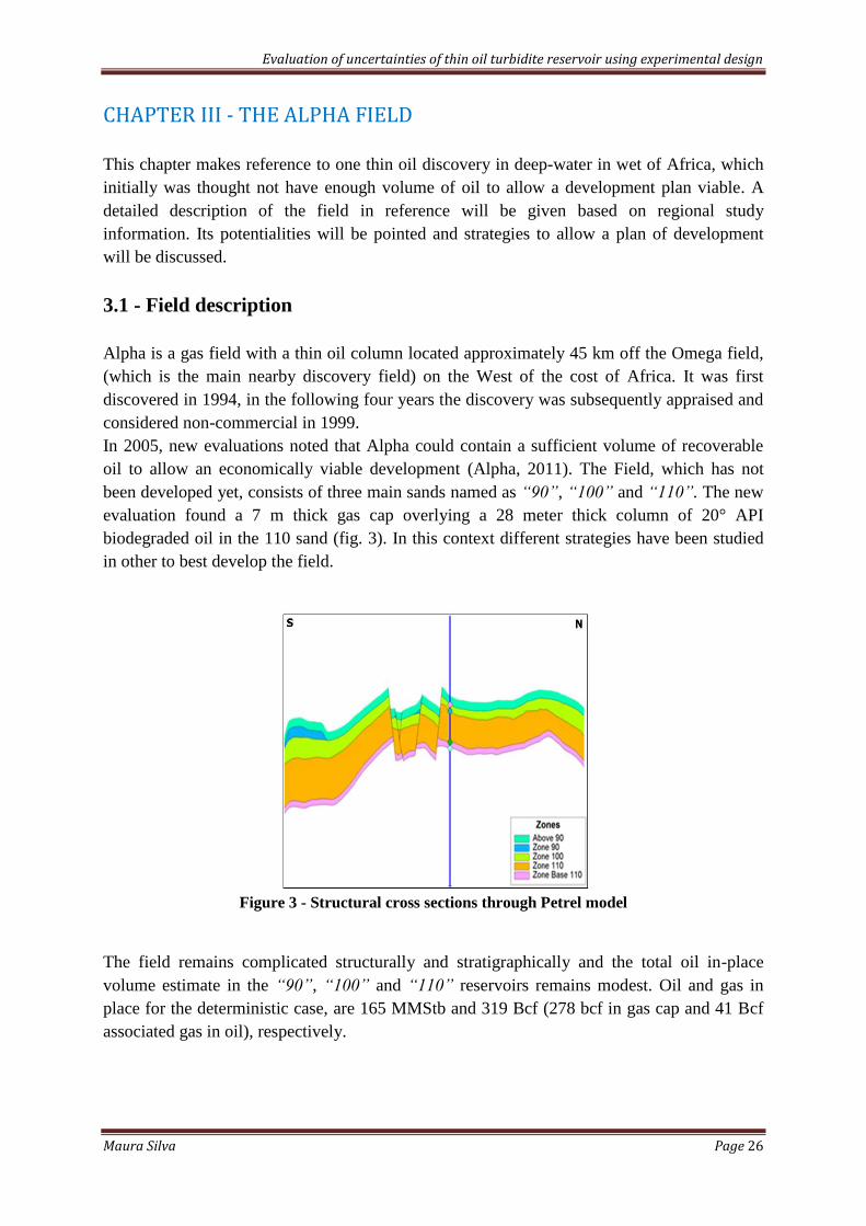
been developed yet, consists of three main sands named as “90”, “100” and “110”. The new
evaluation found a 7 m thick gas cap overlying a 28 meter thick column of 20° API
biodegraded oil in the 110 sand (fig. 3). In this context different strategies have been studied
in other to best develop the field.
Figure 3 - Structural cross sections through Petrel model
The field remains complicated structurally and stratigraphically and the total oil in-place
volume estimate in the “90”, “100” and “110” reservoirs remains modest. Oil and gas in
place for the deterministic case, are 165 MMStb and 319 Bcf (278 bcf in gas cap and 41 Bcf
associated gas in oil), respectively.
Evaluation of uncertainties of thin oil turbidite reservoir using experimental design
Maura Silva Page 27
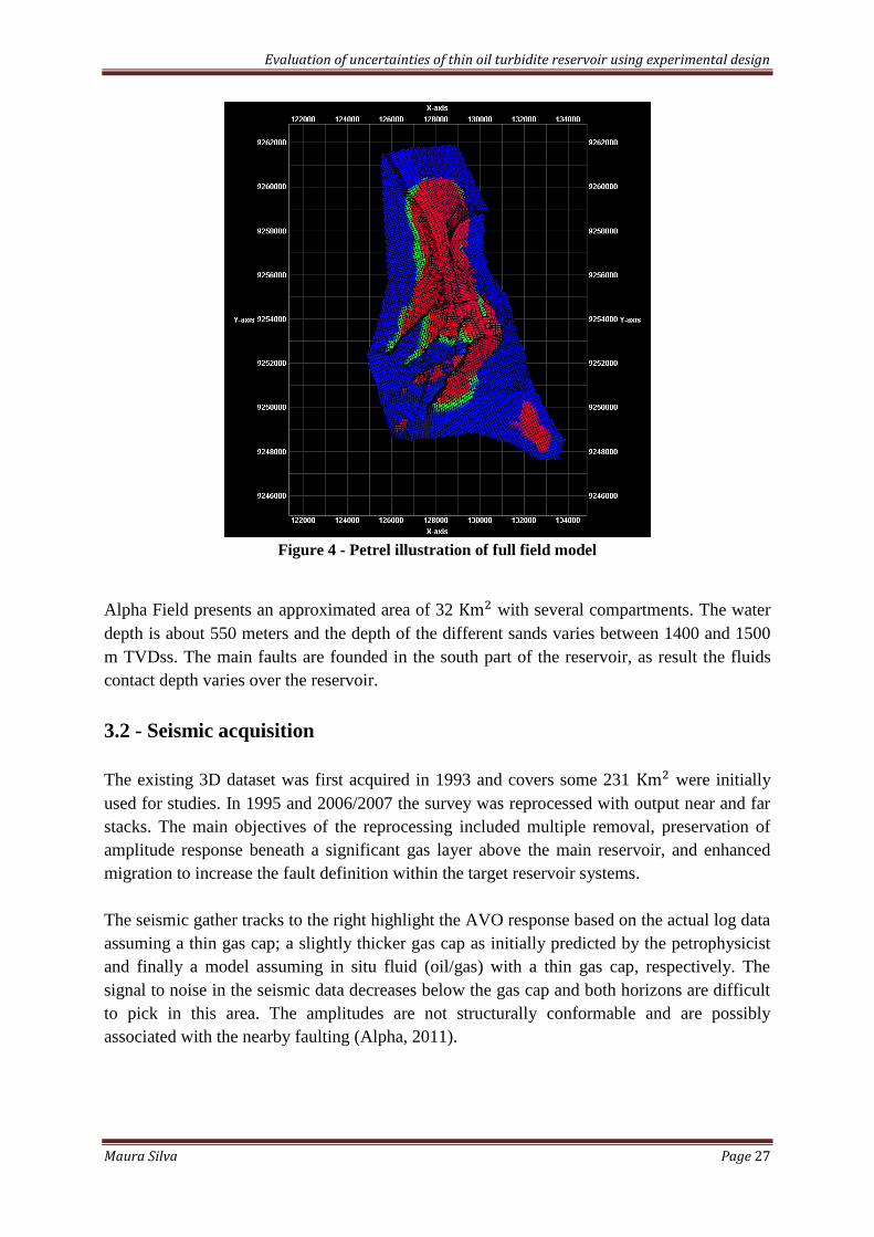
Figure 4 - Petrel illustration of full field model
Alpha Field presents an approximated area of 32 with several compartments. The water
depth is about 550 meters and the depth of the different sands varies between 1400 and 1500
m TVDss. The main faults are founded in the south part of the reservoir, as result the fluids
contact depth varies over the reservoir.
3.2 - Seismic acquisition
The existing 3D dataset was first acquired in 1993 and covers some 231 were initially
used for studies. In 1995 and 2006/2007 the survey was reprocessed with output near and far
stacks. The main objectives of the reprocessing included multiple removal, preservation of
amplitude response beneath a significant gas layer above the main reservoir, and enhanced
migration to increase the fault definition within the target reservoir systems.
The seismic gather tracks to the right highlight the AVO response based on the actual log data
assuming a thin gas cap; a slightly thicker gas cap as initially predicted by the petrophysicist
and finally a model assuming in situ fluid (oil/gas) with a thin gas cap, respectively. The
signal to noise in the seismic data decreases below the gas cap and both horizons are difficult
to pick in this area. The amplitudes are not structurally conformable and are possibly
associated with the nearby faulting (Alpha, 2011).
Evaluation of uncertainties of thin oil turbidite reservoir using experimental design
Maura Silva Page 28
3.3 - Evaluation of depositional environment and burial history
The depositional model for the Alpha reservoir is defined as a fully marine intra-slope or base
of slope environment, characterized by turbiditic sand flows originating from the shelf. Both
confined and unconfined channel systems have been observed, showing that the reservoir is
compartmentalized with different sands along with sheet-like facies indicating considerable
complexity. The natural local deposition was during the Upper and Middle Miocene, which
resulted in to present renewed sub-regional subsidence and raft grounding and initiation of
extreme downdip raft tectonics and continued halokinesis.
The ultimate seal to the alpha hydrocarbon accumulations is the Upper Miocene package
above the “90” and “100” sands. This package, was grey, soft, plastic, homogeneous
claystones with very minor streaks of dolomite, and represents a deep marine depositional
environment (Alpha, 2011).
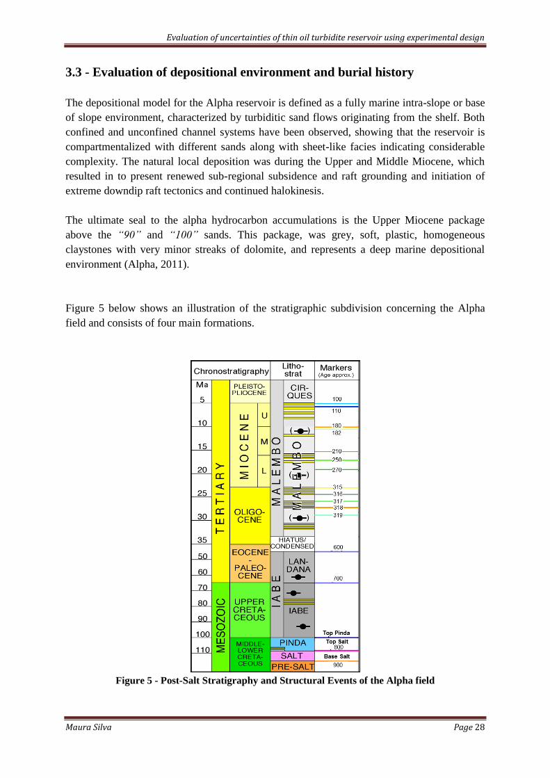
Figure 5 below shows an illustration of the stratigraphic subdivision concerning the Alpha
field and consists of four main formations.
Figure 5 - Post-Salt Stratigraphy and Structural Events of the Alpha field

Evaluation of uncertainties of thin oil turbidite reservoir using experimental design
Maura Silva Page 29
Malembo Formation: Closure of the Tethys and the incipient collision of the Indian and
Asian continents in the Middle Oligocene triggered a significant global tectonic event. The
West African margin was uplifted and eroded, shedding a large quantity of clastics into the
basin. Consequently the basin was gradually filled with a progradational sequence of fluvial,
deltaic to prodeltaic sediments. In the offshore area, a thick pile of deep marine shales and
sandy turbidites was deposited from the Late Oligocene into the Miocene (Alpha, 2011).
Iabe and Landana Formations: Deep marine black shales and bituminous lime mudstones
rich in organic matter were the predominant sediments deposited over the broad slope and
deeper shelf environment (Alpha, 2011).
Pinda formation: Separation of the African and South American continents accelerated
toward the end of the Aptian, leading to a eustatic sea level rise. Normal sea water broke
through the Walvis Ridge and flooded the entire inland basin. Albian carbonates or mixed
carbonates and clastics were accumulated on the shelf initially, but sediment-starved
conditions quickly took over under the rapid marine transgression from the late Cretaceous to
the early Tertiary (Alpha, 2011).
Salt and pre-salt formations: pre-salt and post-salt mega-sequences, separated by the Aptian
salt layer (fig. 5). Some minor early vertical salt movement is believed to have started in the
Albian and Cenomanian locally. Such deformation was closely associated with the
reactivation of the syn-rift faults, and it caused significant local thickness and lithology
variations of the Pinda Formation (Alpha, 2011).
3.3.1 - Geological interpretation
The geological interpretation of the Alpha reservoir systems was based upon seismic
sequence analysis, seismic amplitude, seismic waveform classification and core and log
analysis from the explorations wells (alpha-1 and alpha-2 wells).
Cores samples collected in “110”, “180” and in the “105/110” sands by alpha-1 reveals that
the reservoir sands in all of the cores were fine grained, rich in quartz without clay, fine-
medium grained, and moderate to well sorted. They were mostly massive at alpha-1. At alpha-
2 there were fining up cycles to silty and shaley sandstone. Environments of deposition were
interpreted as channels or sheets at alpha-1 and channel abandonment at alpha-2. The
numerous faults at Alpha opened the possibility that there could be fault
compartmentalization, especially in consideration of the fact that alpha-1 and alpha-2
encountered different fluid contacts. In addition, in the southeast and southwest parts of the
field there were some isolated “90” sand reservoirs which had deeper contacts. From the
seismic response, these appear to contain gas only (Alpha, 2011). The fluids contacts of the
wells were encountered at different depth.

Evaluation of uncertainties of thin oil turbidite reservoir using experimental design
Maura Silva Page 30
Alpha accumulation contains a free gas cap in the “90”, “100” and “110” intervals (as
penetrated by alpha-1 and alpha-2), it is also clear that the post “90” and “100” seal is
effective, despite clear evidence of faulting through the known reservoirs, through the seal
package, and into the shallower sand units above. In addition, shallow gas anomalies
associated with the crest of the Alpha structure indicate some leakage from the hydrocarbon
column (Alpha, 2011).
3.3.2 - Sedimentological reservoir model
Seismic analysis of the “100” and “110” intervals suggests that the reservoir systems are
related, with the “90” interval being the last pulse of coarser clastics from the shelf system
before the onset of deeper water and the dominance of the claystone which forms the present-
day hydrocarbon seal.
Coherency and amplitude extractions indicate that the core of the Alpha field is dominated by
strong, westward oriented, linear, confined turbidities channel systems, which appear to reach
a break in slope outboard of the field and become largely unconfined and more distributary in
nature.
The west of the field is dominated by two large turbidities fan systems, the greater of which
originates in the center of the field and coincides with an observed down-cutting canyon
system that partially erodes the ”100” and ”110” levels. The large fan system was observed
due to a switching confined to unconfined close to the observed oil water contact (OWC).
Above the OWC it would appear that the system is predominantly confined and hence limits
reservoir connectivity in the north-south direction. Below the OWC the reservoirs become
much more like amalgamated channelized sheets with a greater degree of connectivity and
avulsion events (Alpha, 2011).
3.4 - Strategy and developing plan
Different studies have been carrying out to evaluate how would be an optimal strategy for a
developing plan. It was already mentioned that Alpha field is located around 45 km away
from a main field (Omega field) and was initially thought to not have any commercial value.
Therefore, it is important to emphasize that as a thin oil reservoir in deep water, a standalone
would be a commercial challenge. The interest of developing such field is related in adopt
advanced technologies as smart or intelligent wells as well as integrated operations, and thus
extend the life time of the reservoir. As start point engineers have been focused in developing
the field along with the Omega field. In other words both reservoirs (Omega and Alpha)
would be sharing common surface infrastructure and production facilities, which strongly
interlinks its operations. This way some of the costs would be reduced. A tieback
development scenario relies mostly on flow assurance and pipelines issues.
Evaluation of uncertainties of thin oil turbidite reservoir using experimental design
Maura Silva Page 31
3.5 - Uncertainties in the Alpha reservoir data
Given that the Alpha field is in appraisal stage the data gathering process still in progress. The
process is been lengthy, due the limited volume of hydrocarbons encountered in different
compartments around the field. The progress of the process is compounded because it is
located in deep water conditions, where the data collection is a challenge beyond to be costly.
In addition the reservoir itself is stratigraphically complex with multiple reservoir layers
compartments, resulting in drastic changes along the reservoir,( in terms of type of sand
grains, net to gross ratio, permeability heterogeneity, fluids contacts, oil saturation), which
may lead to different scales of uncertainties.
As result some measurements as SCAL, rock compressibility, wettability are not available
and some others are uncertain as permeability. In cases were no SCAL data is available,
important measurements analysis as relative permeability become unknown leading to the use
of information based on generic data and some extent regional knowledge (as verified in the
present work) corresponding to a certain degree of uncertainty. Relative permeability curves
define the reservoir mechanics, and hence, they are vital for describing the depletion method
of any field discovery.
So, it becomes essential to have a consistent and efficient way of incorporating the effect of
uncertain parameters on the behavior of a reservoir and to forecast the probabilistic
production of the reservoir. In this study a screening experimental design is implemented in
order to portray how robust the oil production is to variations in some of the key engineer
parameters, and also highlight which of the inputs parameters is more sensitive to. Ranking
the uncertainties can greatly help to prioritize where resources should be directed to get the
most cost effective investigation.
Evaluation of uncertainties of thin oil turbidite reservoir using experimental design
Maura Silva Page 32
CHAPTER IV – THE SIMULATION MODEL
This chapter gives a more technical description based on availability of data. In the following
are presented some of the key input data of the full model with emphasis on the sector model.
4.1 - Available data
The progress of the entire work was based on a set of existing data provided. The following
data were given:
Regional seismic information
Log analysis
Pressure data
PVT lab measurement
DST
Static and dynamic models
4.2 - Reservoir simulation model
As the reservoir is still in the initial stage of appraisal then many parameters are uncertain.
Therefore, a simulation model was generated based on various deterministic scenarios from
previous studies.
The initial simulation model is actually a Cartesian 3D, black oil simulator ECLIPSE 100 was
developed from the geological model calibrated to seismic data along with some generic data
where data were absent. The simulation model is discretized into 77 by 159 by 51 cells,
making a total of 624,393 grid cells, among them 296,859 are active.
The reservoir formation is upper Miocene with different sands quality and high permeability.
Table 1 gives some of the reservoir property ranges as well as fluids properties, provided by
studies performed during the appraisal phase of the field (Alpha, 2011).
Table 2 - Reservoir and fluids properties
Reservoir properties
Initial pressure, psi 2100
Initial temperature, °C 55 - 60
Reservoir depth, m TVDss 1400
Rock wettability unknown
Formation Upper Miocene
Water Depth, m 500 - 600

Evaluation of uncertainties of thin oil turbidite reservoir using experimental design
Maura Silva Page 33
A three-dimensional view of the entire model with the respective area of interest modeled in
the sector model (area in blue) can be seen in fig. 6. The simulation period started from the
first of January 2016 up to the first of December 2041.
Figure 6 - Alpha field showing the area of Sector Model in blue dark
The regional seismic information indicates that the Alpha accumulation contains a free gas
cap in the main sands intervals (90, 100 and 110). In addition the several channels
encountered in south part of reservoir indicate clearly that the reservoir contains several
Crude Heavy oil biodegradaded
Porosity, % 22 - 38
Permeability (best estimate),
mD
2000
Thickness, m 28
Bubble point pressure, psi 2075
Fluids distribution Gas cap, thin oil, significant aquifer
Reservoir fluids properties
Oil density, g/ 0.8709
Specific gravity (air =1) 0.611
Oil viscosity, cp 4 - 5
Solution GOR, scf/stb 240
Formation volume factor,
rb/stb
1.11
Oil gravity (API) 20
Evaluation of uncertainties of thin oil turbidite reservoir using experimental design
Maura Silva Page 34
sealing faults, which divide the reservoir into different compartments. In the simulation model
those compartments were designated as region with no way of communication with nearby
regions. The simulation model comprises a total of seventeen regions but only one has been
selected. The so-called sector model will receive a special attention in the following sections.
4.2.1 – Sector model
It is well known that a single reservoir simulation could require several hours or even days of
computation time, depending on the size of the reservoir, the numbers of the wells involved,
and the complexity of the physical model to be considered. In this context the sector model
was selected for phenomenological and CPU time studies, where different tests were
performed involving critical rate prediction, impact of grid resolution, sensitivity analyses and
IOR. Since, the present work deals with a thin oil accumulation sandwiched by a gas cap and
bottom water, these studies were quite interesting to investigate the coning progression over
the time as well as to achieve a suitable plan that would lead to a realistic range of outcomes.
As previously mentioned the sector model is basically one of the field compartments, it is
located in the Southwest part of the Alpha field and has a total area of around 6 . The
initial gas in place is about 15% (43 bcf) of the total gas in place and 24% (38MMstb) of total
amount of oil present in the entire field. Its simulation model comprises a total of 31,350
coarse grids blocks with 100x100x3 m in dimensions. A single producer horizontal well was
placed and named P1.
In this work the sector model was considered to be the numerical model reference case
scenario, represented by thin heavy oil column, homogeneous and isotropic reservoir, for
simulating gas and water coning tendency, where P1 was producing for twenty six years as a
horizontal well.
The entire work was performed taking into account P1 well path in the sector model as
reference case. Knowing where the fluid contacts were in the model, the optimization of well
placement was achieved by varying the well’s vertical position within the oil column as
function of the oil recovery. A reasonable well placement was found at height closest WOC.
4.2.2- Model Input Data
Due to large amount of data on the full field model, only a few of the essential parameters are
presented in this report. In the following are presented some of the key input fluid and
reservoir data like formation volume factor oil and gas viscosity, porosity and net to gross
ratio. It is important to emphasize that permeability in the sector model was considered to be
homogeneous as little variation was observed within net sand package in the two wells in the
structure.

Evaluation of uncertainties of thin oil turbidite reservoir using experimental design
Maura Silva Page 35
4.2.2.1 - Fluid data
The fluid properties characterization of the Alpha reservoir was based in a number of
laboratory experiments. To construct a representative fluid data to be used as input to the
dynamic model, a fluid characterization study was generated using the EOS modeling and it
was conducted accordingly with respect to pressure in the simulation input data.
Figures 7 to 10 depict plots of fluid data which are oil formation volume factor (Bo), oil
viscosity (cp), solution, gas formation volume factor (Bg), and gas viscosity data (cp),
respectively.
Figure 7 - Liquid formation volume factor vs. pressure captured from petrel
Figure 8 - Oil viscosity vs. pressure captured from petrel
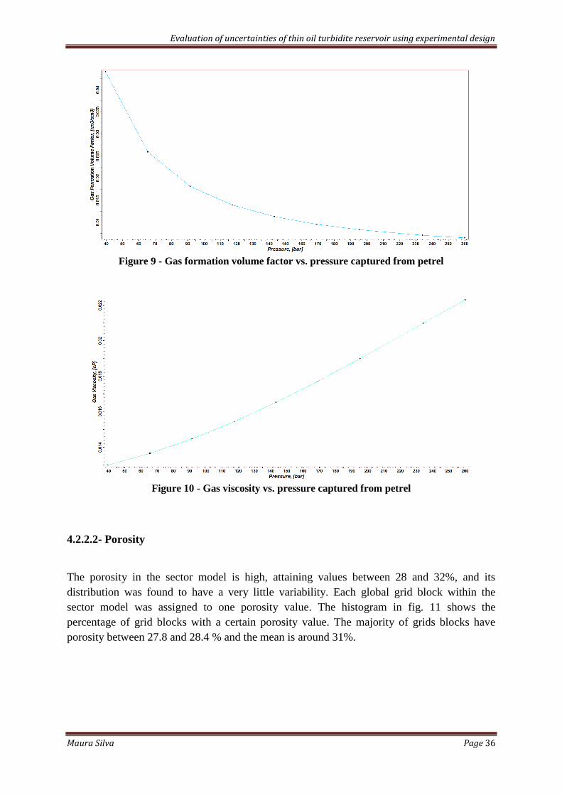
Evaluation of uncertainties of thin oil turbidite reservoir using experimental design
Maura Silva Page 36
Figure 9 - Gas formation volume factor vs. pressure captured from petrel
Figure 10 - Gas viscosity vs. pressure captured from petrel
4.2.2.2- Porosity
The porosity in the sector model is high, attaining values between 28 and 32%, and its
distribution was found to have a very little variability. Each global grid block within the
sector model was assigned to one porosity value. The histogram in fig. 11 shows the
percentage of grid blocks with a certain porosity value. The majority of grids blocks have
porosity between 27.8 and 28.4 % and the mean is around 31%.

Evaluation of uncertainties of thin oil turbidite reservoir using experimental design
Maura Silva Page 37
Figure 11 - Porosity distribution in the model
4.2.2.3-Net to Gross ratio
The Net-to-Gross ratio reveals the quality the height of producible sand relative to the total
thickness; it is usually linked to the accessible length of the appropriated sand in the reservoir,
required to convert from gross to net thickness. The good sands were grouped between 0.95 and 1
and accounted for more than 18 % of the grid blocks. About half of total grid blocks are found
around 0.05 and 0.5. Figure 12 shows the distribution.
Figure 12 - Net-to-Gross ratio distribution in the model
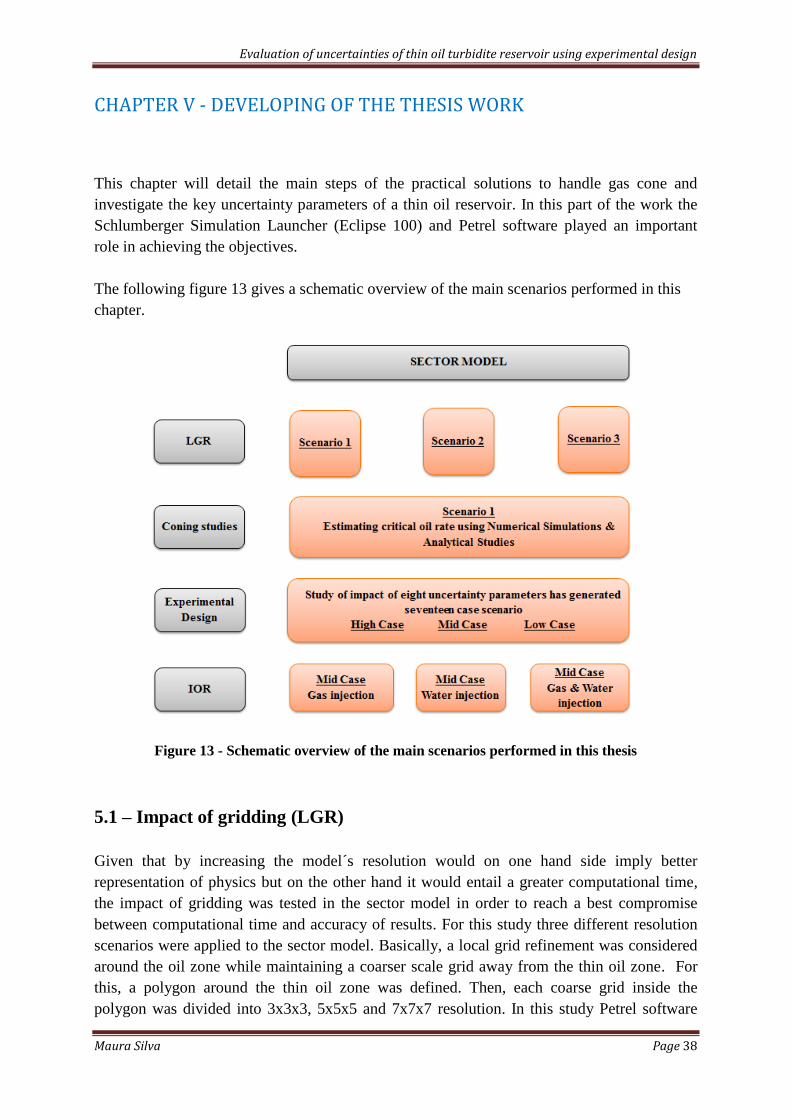
Evaluation of uncertainties of thin oil turbidite reservoir using experimental design
Maura Silva Page 38
CHAPTER V - DEVELOPING OF THE THESIS WORK
This chapter will detail the main steps of the practical solutions to handle gas cone and
investigate the key uncertainty parameters of a thin oil reservoir. In this part of the work the
Schlumberger Simulation Launcher (Eclipse 100) and Petrel software played an important
role in achieving the objectives.
The following figure 13 gives a schematic overview of the main scenarios performed in this
chapter.
Figure 13 - Schematic overview of the main scenarios performed in this thesis
5.1 – Impact of gridding (LGR)
Given that by increasing the model´s resolution would on one hand side imply better
representation of physics but on the other hand it would entail a greater computational time,
the impact of gridding was tested in the sector model in order to reach a best compromise
between computational time and accuracy of results. For this study three different resolution
scenarios were applied to the sector model. Basically, a local grid refinement was considered
around the oil zone while maintaining a coarser scale grid away from the thin oil zone. For
this, a polygon around the thin oil zone was defined. Then, each coarse grid inside the
polygon was divided into 3x3x3, 5x5x5 and 7x7x7 resolution. In this study Petrel software

Evaluation of uncertainties of thin oil turbidite reservoir using experimental design
Maura Silva Page 39
played an important role since, it allows rapid construction of LGR, which made this project
suitable for the limited time available. The scenarios are addressed more in detail in the
following sections.
5.1.1-LGR on an irregular volume
The refinement polygon area was specified in Petrel then exported to Eclipse 100. Therefore,
to perform LGR in ECLIPSE 100 on a volume that is not a regular box the AMALGAM
keyword has been used. By amalgamation smaller refinements could be made along the
wellbore in a zigzag pattern instead of having one single, large LGR box. This way the
amount of local cells and, consequently, simulation time would be reduced. Moreover, this
tool has provided a means of completing a well in more than one local grid. Thus the grid
would be refined more efficiently around a deviated well by employing a number of smaller
refinements.
5.1.2 -Time steps
In general, refined grids often require shorter time steps than coarse grids. Local time stepping
allows each amalgamation to be solved at individual time steps. Two types of time stepping
are available when simulating LGR; namely LGR using local time steps and LGR in-place.
The LGR using local time steps have been used in this study. It is basically an implicit
solution scheme (IMPES method) that Eclipse uses by default, which permits larger time
steps. It is important to take into account that problems related with stability may occur due
the semi-implicit of the method. Despite of the LGR in-place method lead to fully implicit
solution, where the solution of a nonlinear system is required at each time step it may reduce
efficiency of the process.
5.1.3 - Convergence control
Dealing with LGR tool, convergence problems may occur more than usual. Since the number
of cells in the sector model was increased, it also increases the odds that a cell will cause non-
convergence problem. The convergence tolerances are eased slightly at each non-linear
iteration, to make convergence easier as the number of iterations increases. Therefore, to
avoid several convergence problems, during the simulations runs the keyword TUNINGL
were applied along with TUNING. In order to avoid a time-step chop on study of coning the
maximum length of next time step for both global grid and refined grid was set to 0.01 days.
Adjustments on the LITMAX item in both TUNING and TUNINGL keywords were also
considered to improve the performance of the simulator.
5.1.4 -The production well
The horizontal production well here presented measures 2000 meters therefore, the use of a
well with such length in current practice still being investigated. It was considered open hole

Evaluation of uncertainties of thin oil turbidite reservoir using experimental design
Maura Silva Page 40
completed with a production hole of 8,5 inches diameter. A skin value was assumed to be
equal to zero. The well is mainly controlled by bottom hole pressure and rates, which was set
to 100 bars. In order to induce surface constraints, limits target on gas and water was set to
control the volume those fluids to be produced. A favorable vertical placement in the oil
column was considered at 1/3 above OWC. Figure 14 shows the completion and trajectory of
the production well along the layer nine used in all simulations runs.
Figure 14 - Production well trajectory
5.1.5 - Scenario1
Scenario 1 was a case study for a 3x3x3 setting of resolution. It contains 16 amalgamated
local grids, and the maximum number of cells in LGR is 38556. This means that each global
grid was divided into three on the x, y and z directions. In other words Nx=Ny=Nz=3. Figure
15 illustrates a two dimension of the LGR resolutions inside the polygon.
Figure 15 - Illustration of LGR 3x3x3 resolutions inside the polygon used in the model
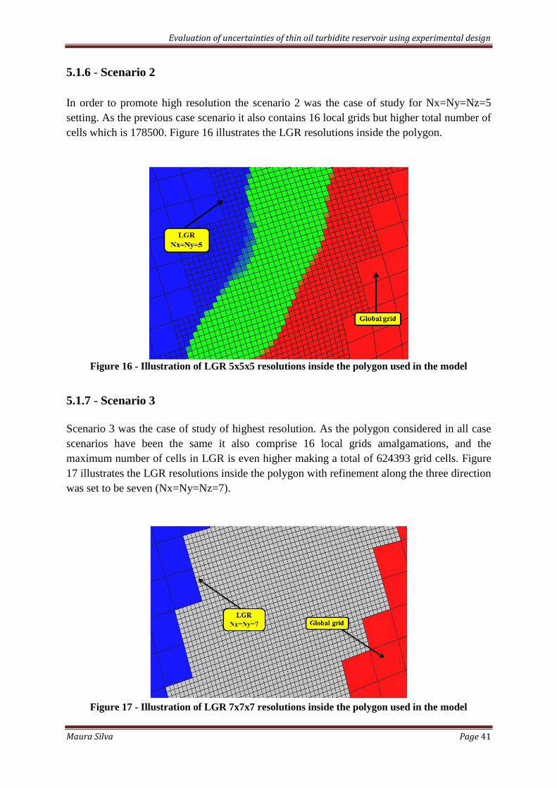
Evaluation of uncertainties of thin oil turbidite reservoir using experimental design
Maura Silva Page 41
5.1.6 - Scenario 2
In order to promote high resolution the scenario 2 was the case of study for Nx=Ny=Nz=5
setting. As the previous case scenario it also contains 16 local grids but higher total number of
cells which is 178500. Figure 16 illustrates the LGR resolutions inside the polygon.
Figure 16 - Illustration of LGR 5x5x5 resolutions inside the polygon used in the model
5.1.7 - Scenario 3
Scenario 3 was the case of study of highest resolution. As the polygon considered in all case
scenarios have been the same it also comprise 16 local grids amalgamations, and the
maximum number of cells in LGR is even higher making a total of 624393 grid cells. Figure
17 illustrates the LGR resolutions inside the polygon with refinement along the three direction
was set to be seven (Nx=Ny=Nz=7).
Figure 17 - Illustration of LGR 7x7x7 resolutions inside the polygon used in the model
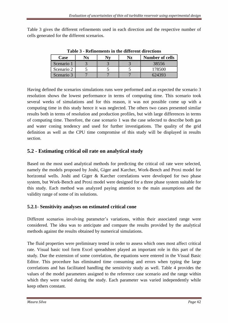
Evaluation of uncertainties of thin oil turbidite reservoir using experimental design
Maura Silva Page 42
Table 3 gives the different refinements used in each direction and the respective number of
cells generated for the different scenarios.
Table 3 - Refinements in the different directions
Case Nx Ny Nz Number of cells
Scenario 1 3 3 3 38556
Scenario 2 5 5 5 178500
Scenario 3 7 7 7 624393
Having defined the scenarios simulations runs were performed and as expected the scenario 3
resolution shows the lowest performance in terms of computing time. This scenario took
several weeks of simulations and for this reason, it was not possible come up with a
computing time in this study hence it was neglected. The others two cases presented similar
results both in terms of resolution and production profiles, but with large differences in terms
of computing time. Therefore, the case scenario 1 was the case selected to describe both gas
and water coning tendency and used for further investigations. The quality of the grid
definition as well as the CPU time compromise of this study will be displayed in results
section.
5.2 - Estimating critical oil rate on analytical study
Based on the most used analytical methods for predicting the critical oil rate were selected,
namely the models proposed by Joshi, Giger and Karcher, Work-Bench and Proxi model for
horizontal wells. Joshi and Giger & Karcher correlations were developed for two phase
system, but Work-Bench and Proxi model were designed for a three phase system suitable for
this study. Each method was analyzed paying attention to the main assumptions and the
validity range of some of its solutions.
5.2.1- Sensitivity analyses on estimated critical cone
Different scenarios involving parameter’s variations, within their associated range were
considered. The idea was to anticipate and compare the results provided by the analytical
methods against the results obtained by numerical simulations.
The fluid properties were preliminary tested in order to assess which ones most affect critical
rate. Visual basic tool form Excel spreadsheet played an important role in this part of the
study. Due the extension of some correlation, the equations were entered in the Visual Basic
Editor. This procedure has eliminated time consuming and errors when typing the large
correlations and has facilitated handling the sensitivity study as well. Table 4 provides the
values of the model parameters assigned to the reference case scenario and the range within
which they were varied during the study. Each parameter was varied independently while
keep others constant.
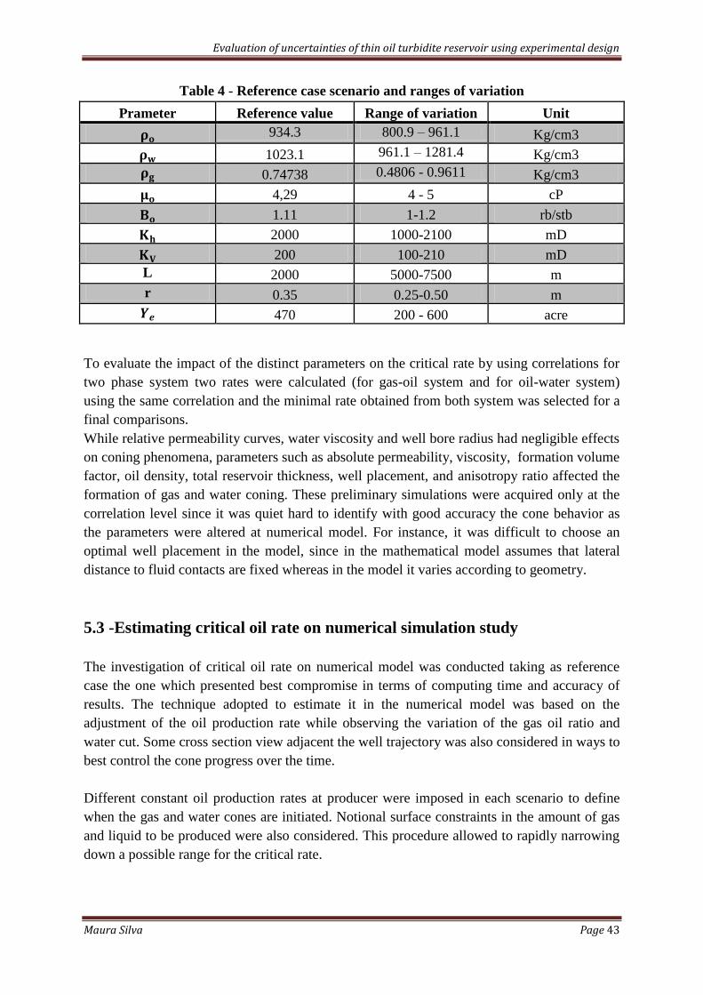
Evaluation of uncertainties of thin oil turbidite reservoir using experimental design
Maura Silva Page 43
Table 4 - Reference case scenario and ranges of variation
Prameter Reference value Range of variation Unit
934.3 800.9 – 961.1 Kg/cm3
1023.1 961.1 – 1281.4 Kg/cm3
0.74738 0.4806 - 0.9611 Kg/cm3
4,29 4 - 5 cP
1.11 1-1.2 rb/stb
2000 1000-2100 mD
200 100-210 mD
L 2000 5000-7500 m
r 0.35 0.25-0.50 m
470 200 - 600 acre
To evaluate the impact of the distinct parameters on the critical rate by using correlations for
two phase system two rates were calculated (for gas-oil system and for oil-water system)
using the same correlation and the minimal rate obtained from both system was selected for a
final comparisons.
While relative permeability curves, water viscosity and well bore radius had negligible effects
on coning phenomena, parameters such as absolute permeability, viscosity, formation volume
factor, oil density, total reservoir thickness, well placement, and anisotropy ratio affected the
formation of gas and water coning. These preliminary simulations were acquired only at the
correlation level since it was quiet hard to identify with good accuracy the cone behavior as
the parameters were altered at numerical model. For instance, it was difficult to choose an
optimal well placement in the model, since in the mathematical model assumes that lateral
distance to fluid contacts are fixed whereas in the model it varies according to geometry.
5.3 -Estimating critical oil rate on numerical simulation study
The investigation of critical oil rate on numerical model was conducted taking as reference
case the one which presented best compromise in terms of computing time and accuracy of
results. The technique adopted to estimate it in the numerical model was based on the
adjustment of the oil production rate while observing the variation of the gas oil ratio and
water cut. Some cross section view adjacent the well trajectory was also considered in ways to
best control the cone progress over the time.
Different constant oil production rates at producer were imposed in each scenario to define
when the gas and water cones are initiated. Notional surface constraints in the amount of gas
and liquid to be produced were also considered. This procedure allowed to rapidly narrowing
down a possible range for the critical rate.

Evaluation of uncertainties of thin oil turbidite reservoir using experimental design
Maura Silva Page 44
5.4 - Uncertainty parameters study
For the uncertainties studies was chose as start point a case that integrated good resolution,
satisfactory computational time and a well producing at estimated critical oil rate (200 ).
Experimental Design technique was applied, but limited to screening phase.
The impact of the chosen uncertainty parameters was evaluated by the variation of each
parameter from its minimum to its maximum values. For this, Petrel software offers a
powerful tool considered of extreme importance in this study; uncertainty and optimization,
tool has several available options to assist the creation of random models. This tool has
permitted select a subset of the combinations of the parameters that provide unambiguous
estimates by run a minimum number of simulations and extract the same information that
could be obtained if every single combination would be considered.
The notional experimental design workflow used in the present work is as followed:
Selecting the uncertainty parameters;
Generate the matrix design table using factorial fractional design method;
Create the ED realizations depending on matrix design;
Perform simulations for all realizations in the ED table;
Import the results to an excel spreadsheet and generate the Pareto plot;
Screen the key parameters from the Pareto plot.
5.4.1 - Selecting the uncertainty parameters
The reason to choose the parameters for this study was based on inexistence of information.
In other words some of data was not available for the Alpha field; therefore generic rock
curves and parameters based on experience and some regional knowledge were used. In the
following are presented the main parameters considered uncertain in this study.
5.4.1.1- Relative permeability
In the absence of actual SCAL for the rock-flow curves, assess the influence of the relative
permeability with an emphasis on the degree of the rock wettability was based considering
different wettabilities.
Three sets of generic relative permeability data were considered representing three different
wettabilities. The oil-wet, weak water-wet and strong water-wet were represented by the low,
mid and high case data sets, respectively. Figure 14 shows the relative permeability curves for
different wettabilities used in this study for water oil system.

Evaluation of uncertainties of thin oil turbidite reservoir using experimental design
Maura Silva Page 45
Figure 18 - Relative Permeability Curves (water-oil system)
5.4.1.2- Horizontal permeability
Both horizontal and vertical permeability were also selected for this study. The permeability
used on previous studies was set to be constant on the intire sector and a reasonabel value to
promote coning prblems. Although a DST was run on a 110 sand interval in the Alpha-1 well
(sector model zone) there is no BHP or WTHP information for the test. BHP or WTHP data is
often used to calibrate permeability and, if run for a sufficient time, can also be used to detect
boundaries and or faults. Since no pressure data was available, the dynamic model used the
horizontal permeability without any calibration. Permeabilities multipliers values rnging from
0,5 to 1,25 were used for this study.
5.4.1.3 - Vertical permeability
A generic vertical permeability of 0.275 for the Permultx mnemonic was used in the mid case
model. Since the core data is very limited and does not suggest a representative degree of
permeability, the influence of anisotropy for this value was investigated. While a low value
was used to incorporate the impact of more shale baffles appearing in the reservoir a high
value was simulated to capture the possibility of a low degree of reservoir anisotropy or the
possibility of holes in shales which would act as vertical conduits to flow.
5.4.1.4 - Aquifer connectivity
It is well perceived that pressure support to the production of reservoir’s hydrocarbons is
critical to the reservoir performance. The efficiency of production wells has the aquifer as a
source of pressure support.
To quantify its effectiveness the connectivity between the aquifer and reservoir was selected
as uncertain parameter to represent both the reasonably low and high sides. The impact of
aquifer on oil production was analyzed by allowing the permeability of certain grid blocks
situated in or near water-oil contacts to vary. This was modeled by applying, to these grid
Evaluation of uncertainties of thin oil turbidite reservoir using experimental design
Maura Silva Page 46
blocks, a pore volume multiplier (MULTPV) of 1, 8 and 15 for the low mid and high cases
respectively.
5.4.1.5 - Rock Compressibility
Being the absence of information the main reason for selecting the uncertain parameters, the
rock mechanics data of the Alpha field were also not available; therefore assumptions were
made to represent the rock compressibility. A typical rock compressibility value of
unconsolidated rock of 0.000217 (at approximately 141 bars) was used in the mid case
model. A range of rock compressibility was assigned 0.0000725 and 0.000435
for the low and high sides respectively.
5.4.1.6 - Well productivity index
Well productivity index reflects the improvement of connectivity between well bore and
formation in terms of degree of damage created during drilling and/or completion of the well.
In order to evaluate the degree of uncertainty for this parameter the permeability in a near-
wellbore area was altered. Multipliers ranging from 0.1 to 10 were used to represent the
possible range of productivity impairment or improvement in the near wellbore area.
5.4.1.7 - Residual oil-to-water saturation
Residual oil saturation is considered as the stranded oil which is capillary trapped in the rock.
The accurate measurement of residual oil saturation is one of the most difficult parameters to
attain in SCAL experiments. In this context a residual oil saturation ranging from 0.1 to 0.25
was used to evaluate its influence on oil production.
5.4.2 - Generating the matrix design table using factorial fractional design method
The case scenario 1 developed in section 5.1.5 (LGR 3x3x3) was set as reference case
scenario and the variables were actually altered based on correspondent Eclipse keyword. In
the context of this study the method was selected with aim of a screening design.
First the variables were defined in Petrel software in order to access the design matrix, where
eight uncertainty parameters have been chosen with low, middle and high values. Table 5
summarizes the ranges in which the parameters have been stretched for this study.
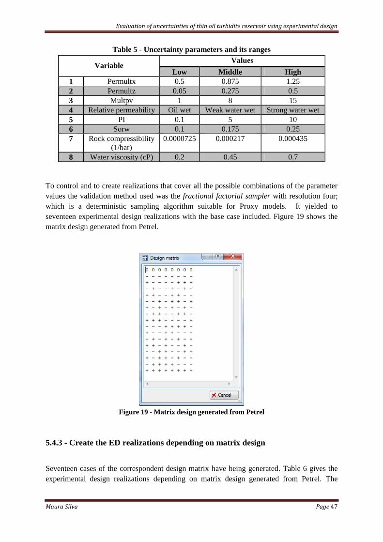
Evaluation of uncertainties of thin oil turbidite reservoir using experimental design
Maura Silva Page 47
Table 5 - Uncertainty parameters and its ranges
Variable Values
Low Middle High
1 Permultx 0.5 0.875 1.25
2 Permultz 0.05 0.275 0.5
3 Multpv 1 8 15
4 Relative permeability Oil wet Weak water wet Strong water wet
5 PI 0.1 5 10
6 Sorw 0.1 0.175 0.25
7 Rock compressibility
(1/bar)
0.0000725 0.000217 0.000435
8 Water viscosity (cP) 0.2 0.45 0.7
To control and to create realizations that cover all the possible combinations of the parameter
values the validation method used was the fractional factorial sampler with resolution four;
which is a deterministic sampling algorithm suitable for Proxy models. It yielded to
seventeen experimental design realizations with the base case included. Figure 19 shows the
matrix design generated from Petrel.
Figure 19 - Matrix design generated from Petrel
5.4.3 - Create the ED realizations depending on matrix design
Seventeen cases of the correspondent design matrix have being generated. Table 6 gives the
experimental design realizations depending on matrix design generated from Petrel. The
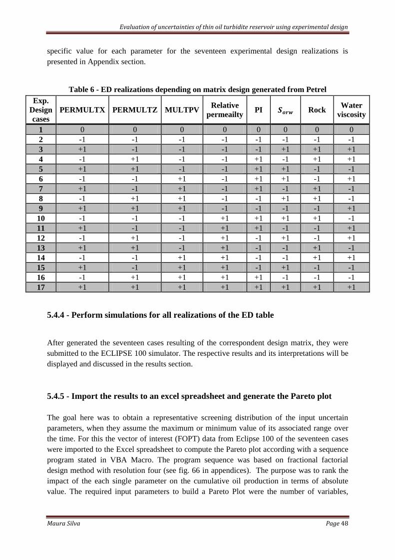
Evaluation of uncertainties of thin oil turbidite reservoir using experimental design
Maura Silva Page 48
specific value for each parameter for the seventeen experimental design realizations is
presented in Appendix section.
Table 6 - ED realizations depending on matrix design generated from Petrel
Exp.
Design
cases
PERMULTX PERMULTZ MULTPV Relative
permeailty PI Rock
Water
viscosity
1 0 0 0 0 0 0 0 0
2 -1 -1 -1 -1 -1 -1 -1 -1
3 +1 -1 -1 -1 -1 +1 +1 +1
4 -1 +1 -1 -1 +1 -1 +1 +1
5 +1 +1 -1 -1 +1 +1 -1 -1
6 -1 -1 +1 -1 +1 +1 -1 +1
7 +1 -1 +1 -1 +1 -1 +1 -1
8 -1 +1 +1 -1 -1 +1 +1 -1
9 +1 +1 +1 -1 -1 -1 -1 +1
10 -1 -1 -1 +1 +1 +1 +1 -1
11 +1 -1 -1 +1 +1 -1 -1 +1
12 -1 +1 -1 +1 -1 +1 -1 +1
13 +1 +1 -1 +1 -1 -1 +1 -1
14 -1 -1 +1 +1 -1 -1 +1 +1
15 +1 -1 +1 +1 -1 +1 -1 -1
16 -1 +1 +1 +1 +1 -1 -1 -1
17 +1 +1 +1 +1 +1 +1 +1 +1
5.4.4 - Perform simulations for all realizations of the ED table
After generated the seventeen cases resulting of the correspondent design matrix, they were
submitted to the ECLIPSE 100 simulator. The respective results and its interpretations will be
displayed and discussed in the results section.
5.4.5 - Import the results to an excel spreadsheet and generate the Pareto plot
The goal here was to obtain a representative screening distribution of the input uncertain
parameters, when they assume the maximum or minimum value of its associated range over
the time. For this the vector of interest (FOPT) data from Eclipse 100 of the seventeen cases
were imported to the Excel spreadsheet to compute the Pareto plot according with a sequence
program stated in VBA Macro. The program sequence was based on fractional factorial
design method with resolution four (see fig. 66 in appendices). The purpose was to rank the
impact of the each single parameter on the cumulative oil production in terms of absolute
value. The required input parameters to build a Pareto Plot were the number of variables,
Evaluation of uncertainties of thin oil turbidite reservoir using experimental design
Maura Silva Page 49
combination of the matrix design provided by Petrel, the number of simulations runs and the
output vector of interest.
5.4.6 - Screening the key parameters from the Pareto plot
A representative screening distribution to assess the impact of the each of the chosen variables
on oil production was achieved. The respective outcome of the screening study is displayed
on the Pareto plot addressed on the results section with respective interpretations.
5.5 - Impact of plateau length by producing above critical rate
In order to access the impact on the plateau length by producing above critical oil rate, the
three main scenarios generated from uncertainty study were considered as low, mid and high
scenarios. The aim of this analysis was to provide an overall view in terms of gains and losses
of reserves when oil companies for economic reasons produce oil as fast as possible. The
results referring to this case will be presented and discussed in the results chapter.
5.6 - Impact of surface constraints on production profiles
Given that specific recovery factor is only valid for a given development concept, in this
particular section the base case generated from experimental design study was simulated
under different gas and water constraints in order to test how the recovery could be affected.
In reality it is linked to the investment proposal on surface capacity. In this context different
scenarios were tested, where only the target limit of unwanted fluids were duplicated and
divided by a factor two. Another case neglecting constraints on the amount of gas and water
allowed to be produced was also considered. On the results section for this study the scenarios
named as high, low and no constraints cases will be presented by Case_Mult, Case_Divid and
Case_No_limit constraints respectively.
5.7 - Improving oil recovery in the sector model
Minimizing the amount of oil recovered in a conventional reservoir is already a challenging
process. It becomes even more complex when it comes to thin oil reservoir with heavy oil
between gas cap and bottom water. As in any reservoir during production it will sooner or
later require pressure maintenance in order to recover as much oil as possible. This study was
conducted under conditions of the mid case generated from experimental design study; where
different scenarios were tested involving gas and water injection wells, placed in different
zones of the sector model in order to support the pressure and thus improve the oil recovery.
Variations on injection rate and test the performance of the injectors at different control mode
were also considered. Therefore, only one case from the each different scenario studied that
yield good results in terms of oil recovery will be presented and compared with the base case.
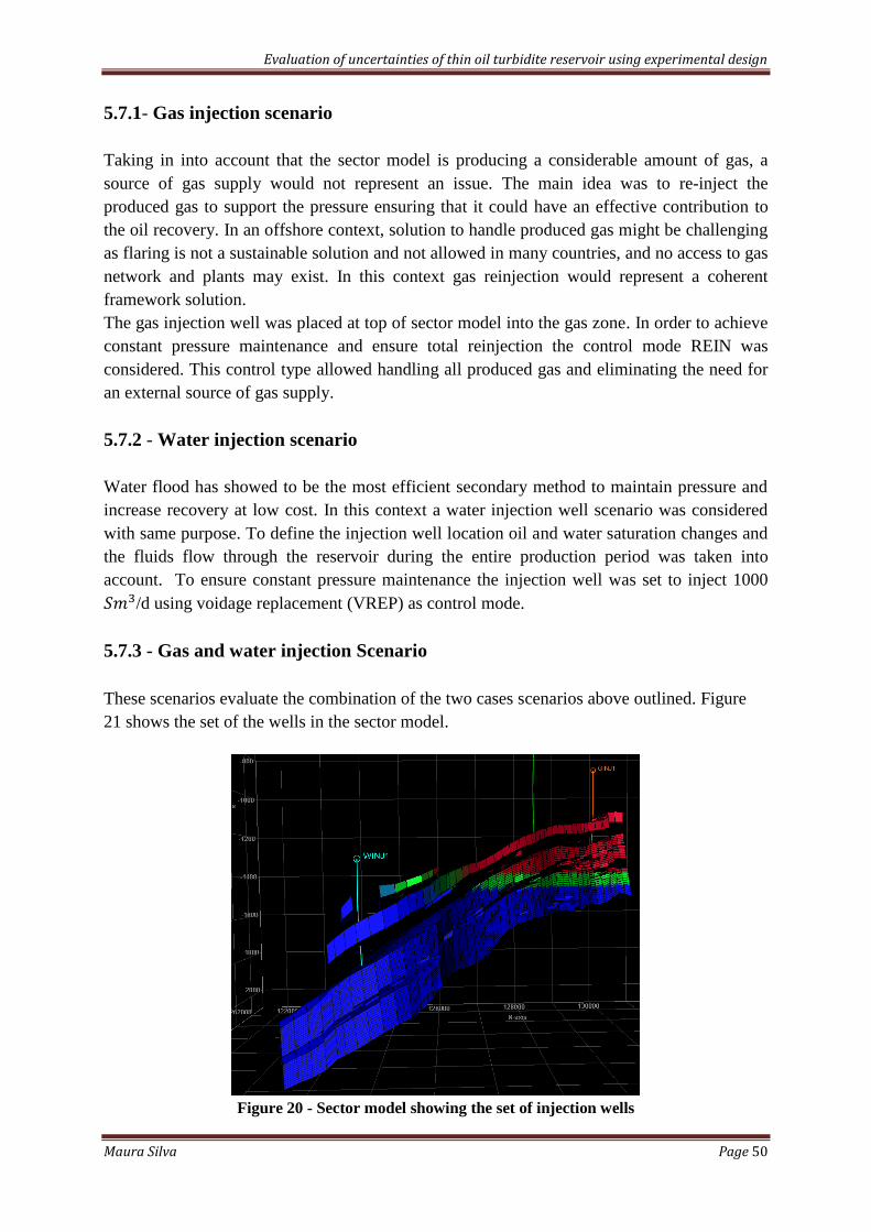
Evaluation of uncertainties of thin oil turbidite reservoir using experimental design
Maura Silva Page 50
5.7.1- Gas injection scenario
Taking in into account that the sector model is producing a considerable amount of gas, a
source of gas supply would not represent an issue. The main idea was to re-inject the
produced gas to support the pressure ensuring that it could have an effective contribution to
the oil recovery. In an offshore context, solution to handle produced gas might be challenging
as flaring is not a sustainable solution and not allowed in many countries, and no access to gas
network and plants may exist. In this context gas reinjection would represent a coherent
framework solution.
The gas injection well was placed at top of sector model into the gas zone. In order to achieve
constant pressure maintenance and ensure total reinjection the control mode REIN was
considered. This control type allowed handling all produced gas and eliminating the need for
an external source of gas supply.
5.7.2 - Water injection scenario
Water flood has showed to be the most efficient secondary method to maintain pressure and
increase recovery at low cost. In this context a water injection well scenario was considered
with same purpose. To define the injection well location oil and water saturation changes and
the fluids flow through the reservoir during the entire production period was taken into
account. To ensure constant pressure maintenance the injection well was set to inject 1000
/d using voidage replacement (VREP) as control mode.
5.7.3 - Gas and water injection Scenario
These scenarios evaluate the combination of the two cases scenarios above outlined. Figure
21 shows the set of the wells in the sector model.
Figure 20 - Sector model showing the set of injection wells
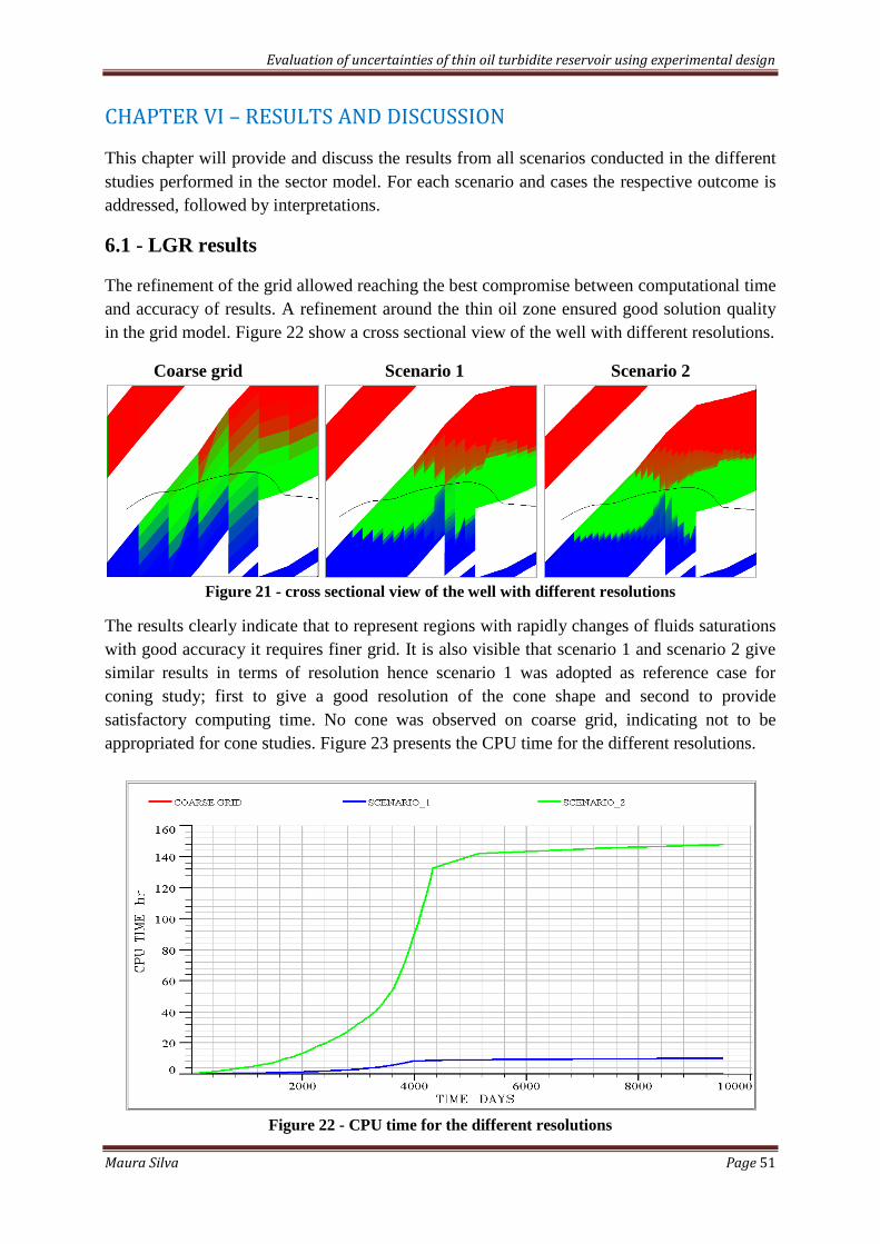
Evaluation of uncertainties of thin oil turbidite reservoir using experimental design
Maura Silva Page 51
CHAPTER VI – RESULTS AND DISCUSSION
This chapter will provide and discuss the results from all scenarios conducted in the different
studies performed in the sector model. For each scenario and cases the respective outcome is
addressed, followed by interpretations.
6.1 - LGR results
The refinement of the grid allowed reaching the best compromise between computational time
and accuracy of results. A refinement around the thin oil zone ensured good solution quality
in the grid model. Figure 22 show a cross sectional view of the well with different resolutions.
Coarse grid Scenario 1 Scenario 2
Figure 21 - cross sectional view of the well with different resolutions
The results clearly indicate that to represent regions with rapidly changes of fluids saturations
with good accuracy it requires finer grid. It is also visible that scenario 1 and scenario 2 give
similar results in terms of resolution hence scenario 1 was adopted as reference case for
coning study; first to give a good resolution of the cone shape and second to provide
satisfactory computing time. No cone was observed on coarse grid, indicating not to be
appropriated for cone studies. Figure 23 presents the CPU time for the different resolutions.
Figure 22 - CPU time for the different resolutions
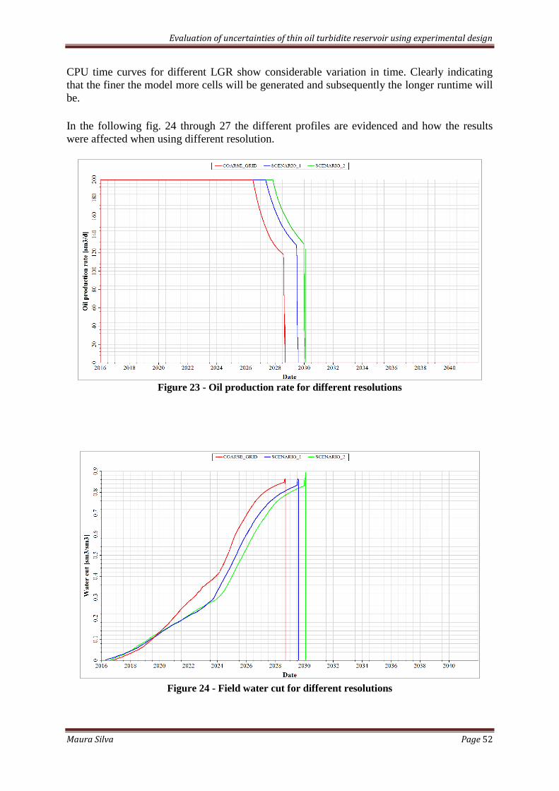
Evaluation of uncertainties of thin oil turbidite reservoir using experimental design
Maura Silva Page 52
CPU time curves for different LGR show considerable variation in time. Clearly indicating
that the finer the model more cells will be generated and subsequently the longer runtime will
be.
In the following fig. 24 through 27 the different profiles are evidenced and how the results
were affected when using different resolution.
Figure 23 - Oil production rate for different resolutions
Figure 24 - Field water cut for different resolutions

Evaluation of uncertainties of thin oil turbidite reservoir using experimental design
Maura Silva Page 53
Figure 25 - Gas oil ratio for different resolution
Figure 26 - field oil production total at different resolution
Based on presented results for this study it is clearly visible that Scenario1 has yielded to the
best compromise between computational time and accuracy of results. Table 7 shows the
recovered volume in barrels and its respective recovery factor for the study above outlined.

Evaluation of uncertainties of thin oil turbidite reservoir using experimental design
Maura Silva Page 54
Table 7 - Recovery factor for study of resolution
Case of study Recovered volume
(MMbbl)
Recovery Factor
(%)
Coarse Grid 5,5 16,2
Scenario_1 6,0 17,5
Scenario_2 6,2 18,2
The cross sections are useful for capturing the cone shape and control its progress over time.
Figure 28 represents the west to east cross section view, how the coning progress over the
time.
Figure 27- Cross section view of the coning progress over the time
This study has allowed verifying that gridding effects, leaded to a satisfactory saturations
disposition and a better resolution of the fluids variation at the model level.
A conclusion that can be taken from this study is that increasing grid resolution improves the
coning interpretation and provides good accuracy on results but the process can be very time
consuming. Therefore, a good compromise between computational time accuracy of results
was achieved.
6.2 - Analytical study results
6.2.1- Critical rate
The analytical and numerical models were used to estimate the critical oil rates based on the
real reservoir characteristics. The ranges of estimated critical rate obtained for correlations
where encountered when varying the parameters evaluated in the sensitivity study. The
response of the numerical model was taken as a reference, so the results obtained with the
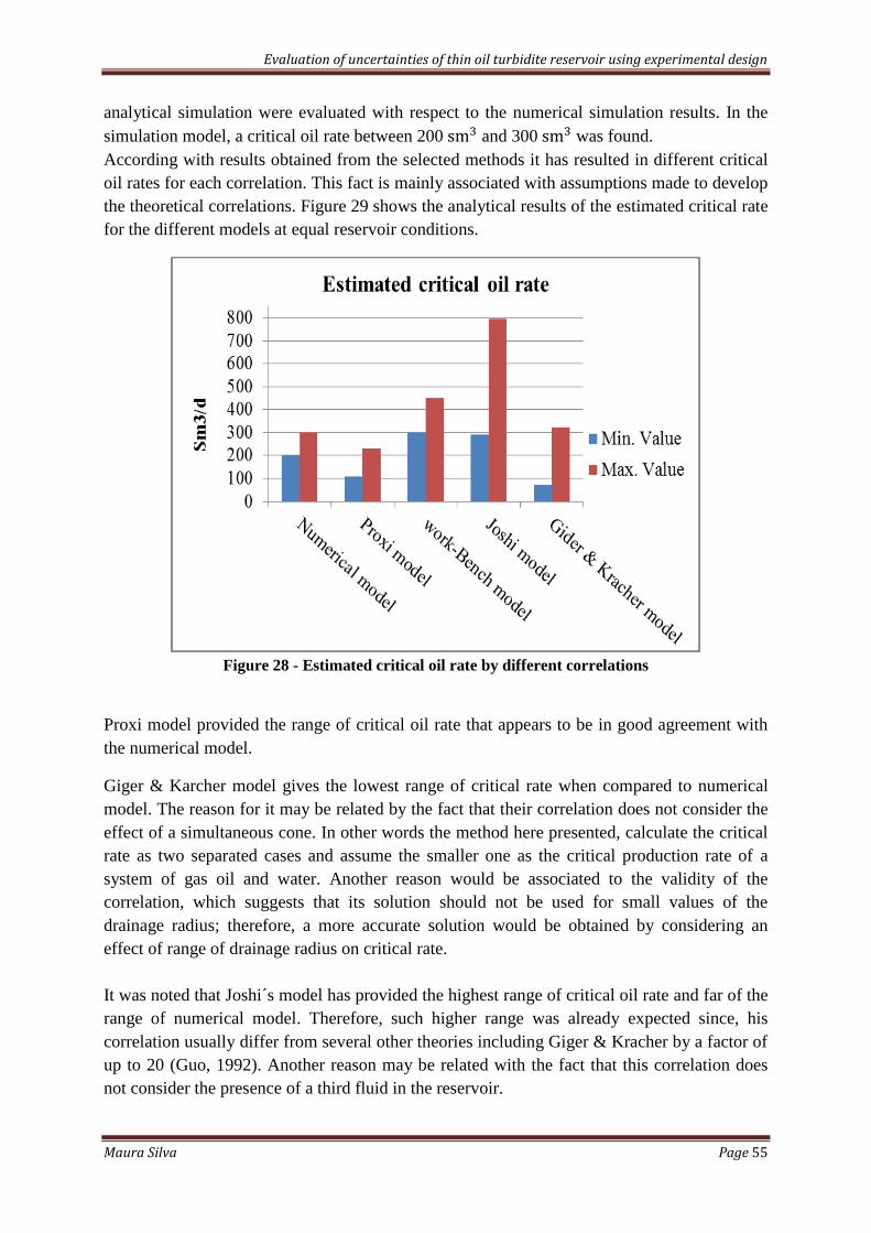
Evaluation of uncertainties of thin oil turbidite reservoir using experimental design
Maura Silva Page 55
analytical simulation were evaluated with respect to the numerical simulation results. In the
simulation model, a critical oil rate between 200 and 300 was found.
According with results obtained from the selected methods it has resulted in different critical
oil rates for each correlation. This fact is mainly associated with assumptions made to develop
the theoretical correlations. Figure 29 shows the analytical results of the estimated critical rate
for the different models at equal reservoir conditions.
Figure 28 - Estimated critical oil rate by different correlations
Proxi model provided the range of critical oil rate that appears to be in good agreement with
the numerical model.
Giger & Karcher model gives the lowest range of critical rate when compared to numerical
model. The reason for it may be related by the fact that their correlation does not consider the
effect of a simultaneous cone. In other words the method here presented, calculate the critical
rate as two separated cases and assume the smaller one as the critical production rate of a
system of gas oil and water. Another reason would be associated to the validity of the
correlation, which suggests that its solution should not be used for small values of the
drainage radius; therefore, a more accurate solution would be obtained by considering an
effect of range of drainage radius on critical rate.
It was noted that Joshi´s model has provided the highest range of critical oil rate and far of the
range of numerical model. Therefore, such higher range was already expected since, his
correlation usually differ from several other theories including Giger & Kracher by a factor of
up to 20 (Guo, 1992). Another reason may be related with the fact that this correlation does
not consider the presence of a third fluid in the reservoir.
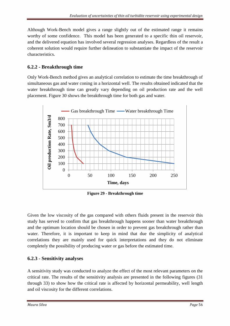
Evaluation of uncertainties of thin oil turbidite reservoir using experimental design
Maura Silva Page 56
Although Work-Bench model gives a range slightly out of the estimated range it remains
worthy of some confidence. This model has been generated to a specific thin oil reservoir,
and the delivered equation has involved several regression analyses. Regardless of the result a
coherent solution would require further delineation to substantiate the impact of the reservoir
characteristics.
6.2.2 - Breakthrough time
Only Work-Bench method gives an analytical correlation to estimate the time breakthrough of
simultaneous gas and water coning in a horizontal well. The results obtained indicated that the
water breakthrough time can greatly vary depending on oil production rate and the well
placement. Figure 30 shows the breakthrough time for both gas and water.
Figure 29 - Breakthrough time
Given the low viscosity of the gas compared with others fluids present in the reservoir this
study has served to confirm that gas breakthrough happens sooner than water breakthrough
and the optimum location should be chosen in order to prevent gas breakthrough rather than
water. Therefore, it is important to keep in mind that due the simplicity of analytical
correlations they are mainly used for quick interpretations and they do not eliminate
completely the possibility of producing water or gas before the estimated time.
6.2.3 - Sensitivity analyses
A sensitivity study was conducted to analyze the effect of the most relevant parameters on the
critical rate. The results of the sensitivity analysis are presented in the following figures (31
through 33) to show how the critical rate is affected by horizontal permeability, well length
and oil viscosity for the different correlations.
0
100
200
300
400
500
600
700
800
0 50 100 150 200 250
Oil
pro
du
ctio
n R
ate
, S
m3/d
Time, days
Gas breakthrough Time Water breakthrough Time

Evaluation of uncertainties of thin oil turbidite reservoir using experimental design
Maura Silva Page 57
Figure 30 - Critical oil rate as a function of horizontal permeability
As it can be seen all methods have similar trend for critical rate. They increase slightly as
horizontal permeability and well length increases, and almost constant as oil viscosity
decreases. With exception of the Joshi method that shows an abrupt and different variation in
all cases.
Figure 31- Critical oil rates calculated as a function of the well length
Work-Bench correlation shows not to be too sensitive for the chosen intervals for both well
length and oil viscosity parameters since it yielded to a variation almost constant on sensitive
study.
50
150
250
350
450
550
650
880 1380 1880
Cri
tica
l R
ate
, S
m3
/d
Horizontal Permeability, mD
Proxi model
Work-Bench
Joshi Method
Giger & Karcher
50
150
250
350
450
550
650
750
850
1500 2000 2500
Cri
tica
l R
ate
, S
m3/d
Well Length, m
Proxi model
Work-Bench
Joshi Method
Giger & Karcher
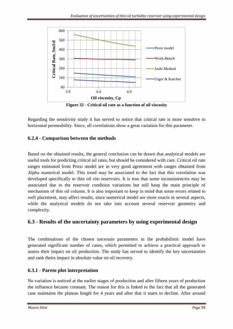
Evaluation of uncertainties of thin oil turbidite reservoir using experimental design
Maura Silva Page 58
Figure 32 - Critical oil rate as a function of oil viscosity
Regarding the sensitivity study it has served to notice that critical rate is more sensitive to
horizontal permeability. Since, all correlations show a great variation for this parameter.
6.2.4 - Comparison between the methods
Based on the obtained results, the general conclusion can be drawn that analytical models are
useful tools for predicting critical oil rates, but should be considered with care. Critical oil rate
ranges estimated from Proxi model are in very good agreement with ranges obtained from
Alpha numerical model. This trend may be associated to the fact that this correlation was
developed specifically to thin oil rim reservoirs. It is true that some inconsistencies may be
associated due to the reservoir condition variations but still keep the main principle of
mechanism of thin oil column. It is also important to keep in mind that some errors related to
well placement, may affect results, since numerical model are more exacts in several aspects,
while the analytical models do not take into account several reservoir geometry and
complexity.
6.3 - Results of the uncertainty parameters by using experimental design
The combinations of the chosen uncertain parameters in the probabilistic model have
generated significant number of cases, which permitted to achieve a practical approach to
assess their impact on oil production. The study has served to identify the key uncertainties
and rank theirs impact in absolute value on oil recovery.
6.3.1 - Pareto plot interpretation
No variation is noticed at the earlier stages of production and after fifteen years of production
the influence became constant. The reason for this is linked to the fact that all the generated
case maintains the plateau length for 4 years and after that it starts to decline. After around
60
160
260
360
460
560
660
3.9 4.4 4.9
Cri
tica
l R
ate
, S
m3
/d
Oil viscosity, Cp
Proxi model
Work-Bench
Joshi Method
Giger & Karcher

Evaluation of uncertainties of thin oil turbidite reservoir using experimental design
Maura Silva Page 59
fifteen years of production, influence became almost stable in most of the cases as the well
stopped producing. Indeed BHP has reached its limit so just few of them still producing for
this reason the variation at the last years of production on Pareto plot is slightly constant.
Figure 34 shows the impact of uncertainties on oil recovery on a Pareto plot.
Figure 33 - Impact of uncertainties on oil recovery on Pareto plot
MULTPV and residual oil on water saturation parameters present a different tend between
the years 2025 and 2028, indicating that at this stage of production these parameters do not
affect significantly the oil production.
Figures 34, 35 and 36 show oil production rate, gas oil ratio and oil production cumulative
over the years of the seventeen ED realizations.
-2.0E+04
3.0E+04
8.0E+04
1.3E+05
1.8E+05
2017
2019
2021
2023
2025
2027
2029
2031
2033
2035
2037
2039
2041
Vari
an
ce i
n o
il r
ecover
y f
rom
min
to m
ax
valu
e (-
1/+
1),
sm
3
Date
Impact of uncertainties on Oil Recovery
Pareto Plot
MULTPV
PERMULTX
PERMULTZ
PI
RELPERM
ROCK
SORW
WATER_VISCOSITY
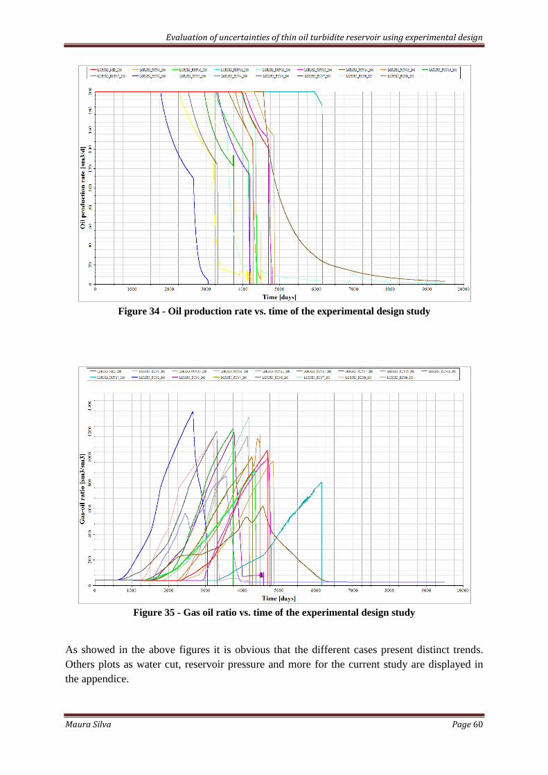
Evaluation of uncertainties of thin oil turbidite reservoir using experimental design
Maura Silva Page 60
Figure 34 - Oil production rate vs. time of the experimental design study
Figure 35 - Gas oil ratio vs. time of the experimental design study
As showed in the above figures it is obvious that the different cases present distinct trends.
Others plots as water cut, reservoir pressure and more for the current study are displayed in
the appendice.
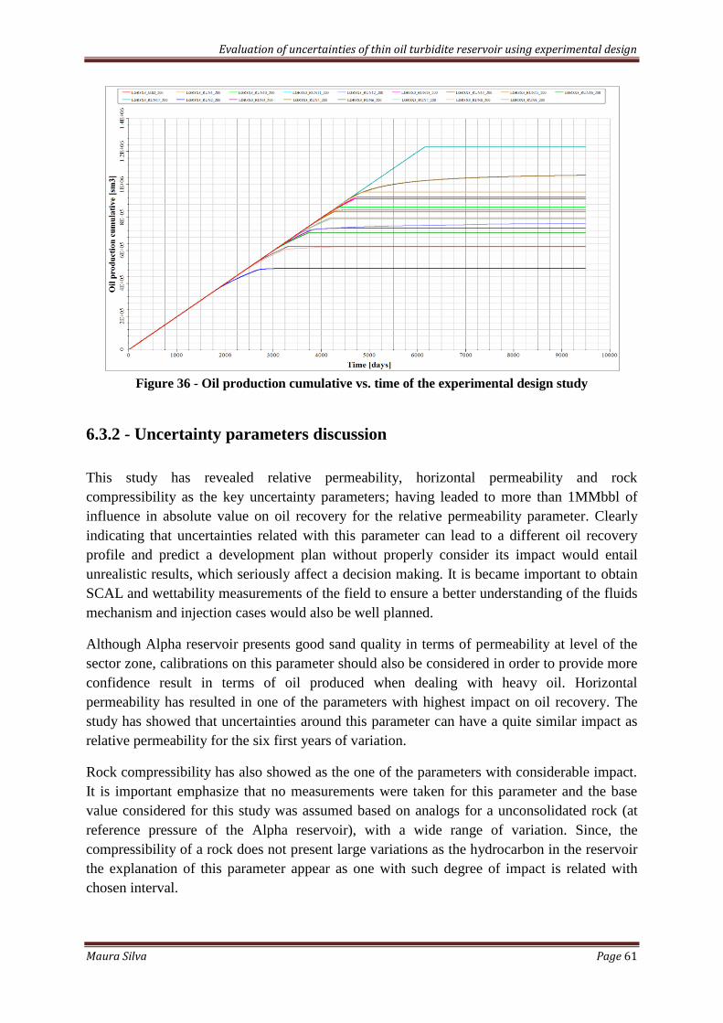
Evaluation of uncertainties of thin oil turbidite reservoir using experimental design
Maura Silva Page 61
Figure 36 - Oil production cumulative vs. time of the experimental design study
6.3.2 - Uncertainty parameters discussion
This study has revealed relative permeability, horizontal permeability and rock
compressibility as the key uncertainty parameters; having leaded to more than 1MMbbl of
influence in absolute value on oil recovery for the relative permeability parameter. Clearly
indicating that uncertainties related with this parameter can lead to a different oil recovery
profile and predict a development plan without properly consider its impact would entail
unrealistic results, which seriously affect a decision making. It is became important to obtain
SCAL and wettability measurements of the field to ensure a better understanding of the fluids
mechanism and injection cases would also be well planned.
Although Alpha reservoir presents good sand quality in terms of permeability at level of the
sector zone, calibrations on this parameter should also be considered in order to provide more
confidence result in terms of oil produced when dealing with heavy oil. Horizontal
permeability has resulted in one of the parameters with highest impact on oil recovery. The
study has showed that uncertainties around this parameter can have a quite similar impact as
relative permeability for the six first years of variation.
Rock compressibility has also showed as the one of the parameters with considerable impact.
It is important emphasize that no measurements were taken for this parameter and the base
value considered for this study was assumed based on analogs for a unconsolidated rock (at
reference pressure of the Alpha reservoir), with a wide range of variation. Since, the
compressibility of a rock does not present large variations as the hydrocarbon in the reservoir
the explanation of this parameter appear as one with such degree of impact is related with
chosen interval.
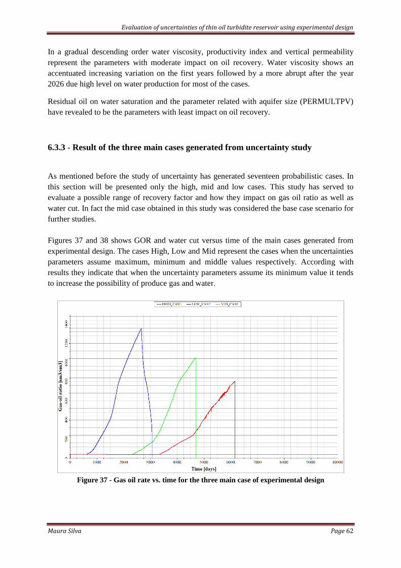
Evaluation of uncertainties of thin oil turbidite reservoir using experimental design
Maura Silva Page 62
In a gradual descending order water viscosity, productivity index and vertical permeability
represent the parameters with moderate impact on oil recovery. Water viscosity shows an
accentuated increasing variation on the first years followed by a more abrupt after the year
2026 due high level on water production for most of the cases.
Residual oil on water saturation and the parameter related with aquifer size (PERMULTPV)
have revealed to be the parameters with least impact on oil recovery.
6.3.3 - Result of the three main cases generated from uncertainty study
As mentioned before the study of uncertainty has generated seventeen probabilistic cases. In
this section will be presented only the high, mid and low cases. This study has served to
evaluate a possible range of recovery factor and how they impact on gas oil ratio as well as
water cut. In fact the mid case obtained in this study was considered the base case scenario for
further studies.
Figures 37 and 38 shows GOR and water cut versus time of the main cases generated from
experimental design. The cases High, Low and Mid represent the cases when the uncertainties
parameters assume maximum, minimum and middle values respectively. According with
results they indicate that when the uncertainty parameters assume its minimum value it tends
to increase the possibility of produce gas and water.
Figure 37 - Gas oil rate vs. time for the three main case of experimental design
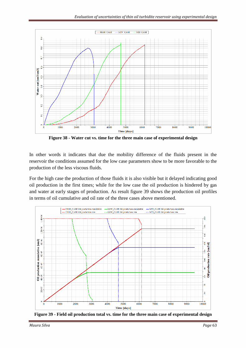
Evaluation of uncertainties of thin oil turbidite reservoir using experimental design
Maura Silva Page 63
Figure 38 - Water cut vs. time for the three main case of experimental design
In other words it indicates that due the mobility difference of the fluids present in the
reservoir the conditions assumed for the low case parameters show to be more favorable to the
production of the less viscous fluids.
For the high case the production of those fluids it is also visible but it delayed indicating good
oil production in the first times; while for the low case the oil production is hindered by gas
and water at early stages of production. As result figure 39 shows the production oil profiles
in terms of oil cumulative and oil rate of the three cases above mentioned.
Figure 39 - Field oil production total vs. time for the three main case of experimental design

Evaluation of uncertainties of thin oil turbidite reservoir using experimental design
Maura Silva Page 64
The three cases yielded to 9%, 17% and 23% of recovery factor for the low, mid and high
case respectively. Table 8 shows the recovered volume in barrels and its respective recovery
factor.
Table 8 - Recovered volume in barrels and recovery factor
Case of study Recovered volume
(MMbbl)
Recovery Factor
(%)
Low Case 3.1 9
Mid Case (Base case) 5.8 17
High Case 7.7 23
6.3.4 - Results of impact on plateau length by producing above critical rate
The study of the impact of plateau has served to evaluate the plateau length and an interval of
recovery when producing above critical rate. Figures 40 and 41 show the possible plateau
length and the respective oil recovery of the three main cases generated from experimental
design study, when they produce above critical oil rate (1000 ).
Figure 40 - Field oil production rate vs. time for the three main case of experimental design
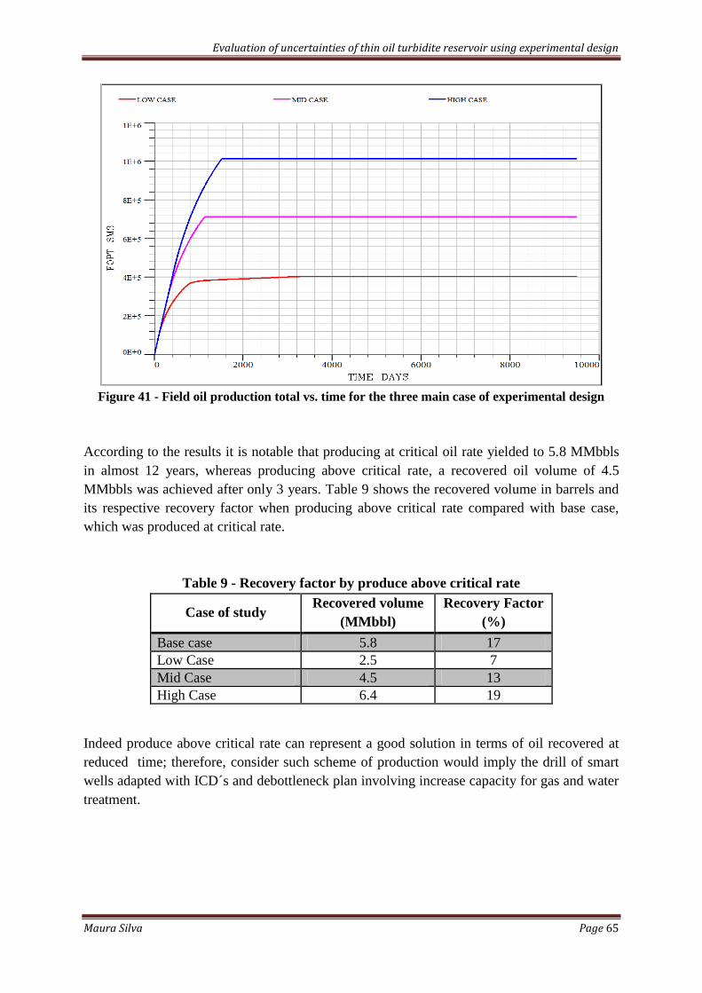
Evaluation of uncertainties of thin oil turbidite reservoir using experimental design
Maura Silva Page 65
Figure 41 - Field oil production total vs. time for the three main case of experimental design
According to the results it is notable that producing at critical oil rate yielded to 5.8 MMbbls
in almost 12 years, whereas producing above critical rate, a recovered oil volume of 4.5
MMbbls was achieved after only 3 years. Table 9 shows the recovered volume in barrels and
its respective recovery factor when producing above critical rate compared with base case,
which was produced at critical rate.
Table 9 - Recovery factor by produce above critical rate
Case of study Recovered volume
(MMbbl)
Recovery Factor
(%)
Base case 5.8 17
Low Case 2.5 7
Mid Case 4.5 13
High Case 6.4 19
Indeed produce above critical rate can represent a good solution in terms of oil recovered at
reduced time; therefore, consider such scheme of production would imply the drill of smart
wells adapted with ICD´s and debottleneck plan involving increase capacity for gas and water
treatment.
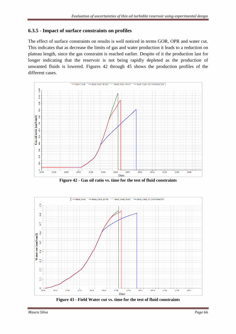
Evaluation of uncertainties of thin oil turbidite reservoir using experimental design
Maura Silva Page 66
6.3.5 - Impact of surface constraints on profiles
The effect of surface constraints on results is well noticed in terms GOR, OPR and water cut.
This indicates that as decrease the limits of gas and water production it leads to a reduction on
plateau length, since the gas constraint is reached earlier. Despite of it the production last for
longer indicating that the reservoir is not being rapidly depleted as the production of
unwanted fluids is lowered. Figures 42 through 45 shows the production profiles of the
different cases.
Figure 42 - Gas oil ratio vs. time for the test of fluid constraints
Figure 43 - Field Water cut vs. time for the test of fluid constraints
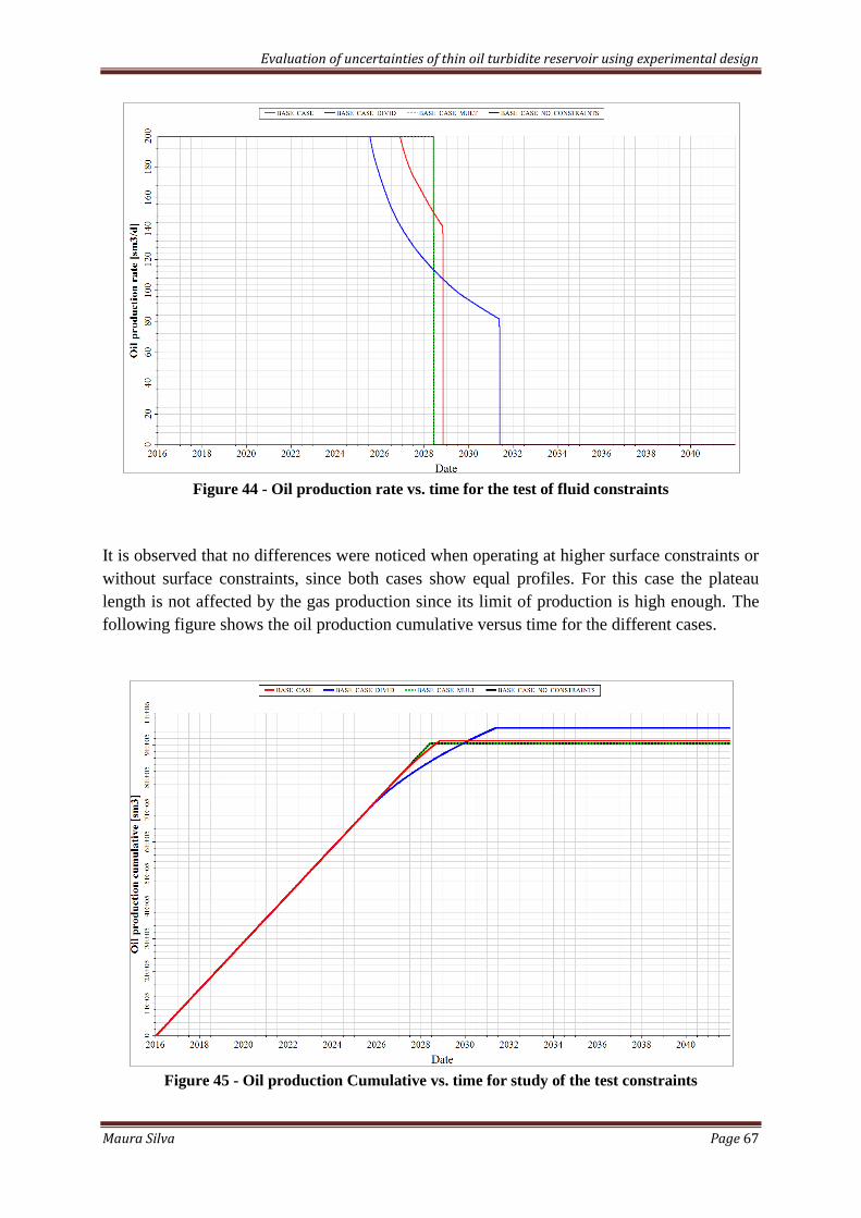
Evaluation of uncertainties of thin oil turbidite reservoir using experimental design
Maura Silva Page 67
Figure 44 - Oil production rate vs. time for the test of fluid constraints
It is observed that no differences were noticed when operating at higher surface constraints or
without surface constraints, since both cases show equal profiles. For this case the plateau
length is not affected by the gas production since its limit of production is high enough. The
following figure shows the oil production cumulative versus time for the different cases.
Figure 45 - Oil production Cumulative vs. time for study of the test constraints

Evaluation of uncertainties of thin oil turbidite reservoir using experimental design
Maura Silva Page 68
According with results decreasing surface constraints leaded to an increasing on oil recovery
of 18%. Table 10 shows the recovered volume in barrels and its respective recovery factor
when surface constraints are altered.
Table 10 - Recovery factor by varying surface constraints
Case of study Recovered volume
(MMbbl)
Recovery Factor
(%)
Base Case 5.8 17
Base Case_ No limit constraints 5.7 16.7
Case_Low surface constraints 6.0 18
Case_High surface constraints 5.7 16.7
6.4 - Results of IOR
6.4.1 - Gas injection scenario
The conditions implemented on injection well for this scenario yielded satisfactory results. In
fact the control mode stated, has positively contributed achieving the expected results. Figures
46 through 51 are presented the different profiles obtained in this study compared with the
reference case.
Figure 46 - field oil production rate vs. time for gas injection scenario
Although the plateau last less than Mid case scenario (Base case) it produces for longer time
as expecting confirming the pressure maintenance of gas injection as showed in figure 49. For
Base case it stops due the low BHP verified on production well when pressure maintenance
was not implemented. The reason why the plateau length is shorter than base case scenario it
is due to gas constraints. In other words for the injection case it was expected to produce more
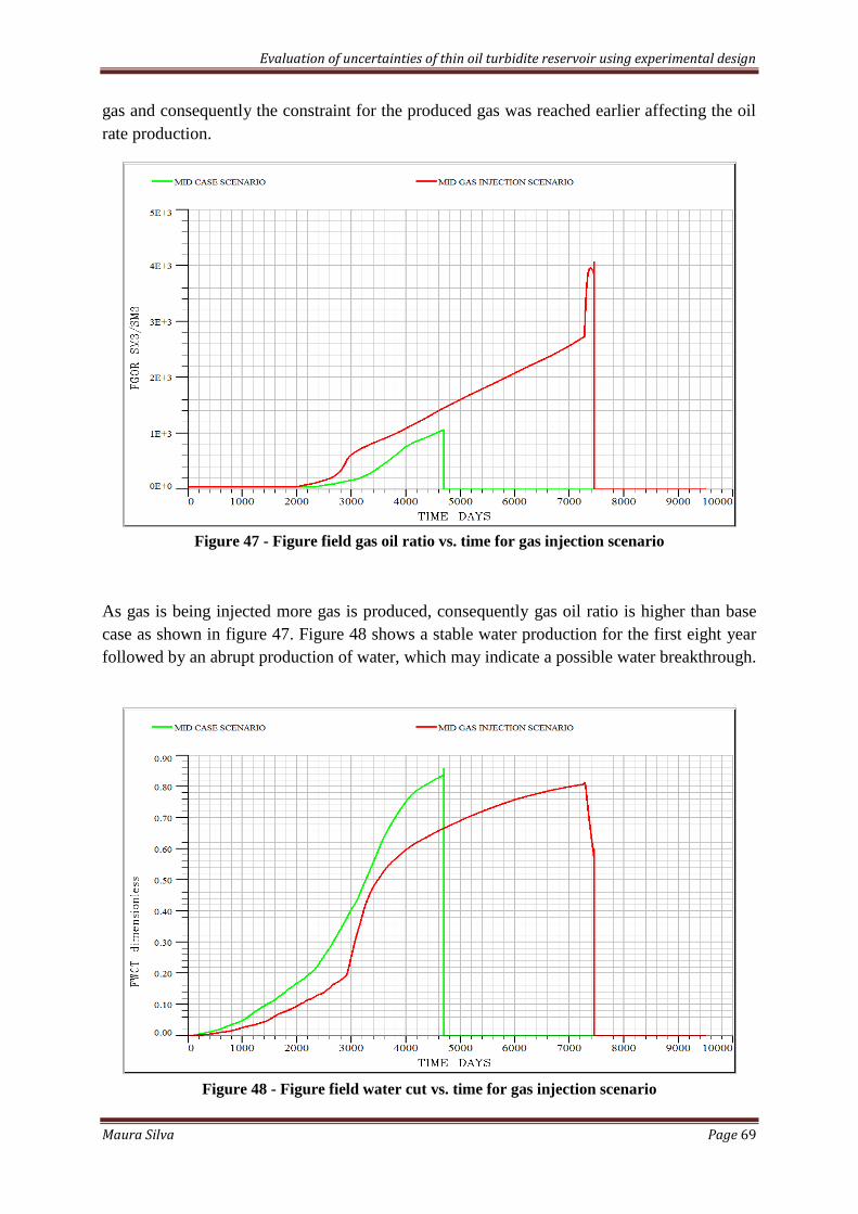
Evaluation of uncertainties of thin oil turbidite reservoir using experimental design
Maura Silva Page 69
gas and consequently the constraint for the produced gas was reached earlier affecting the oil
rate production.
Figure 47 - Figure field gas oil ratio vs. time for gas injection scenario
As gas is being injected more gas is produced, consequently gas oil ratio is higher than base
case as shown in figure 47. Figure 48 shows a stable water production for the first eight year
followed by an abrupt production of water, which may indicate a possible water breakthrough.
Figure 48 - Figure field water cut vs. time for gas injection scenario
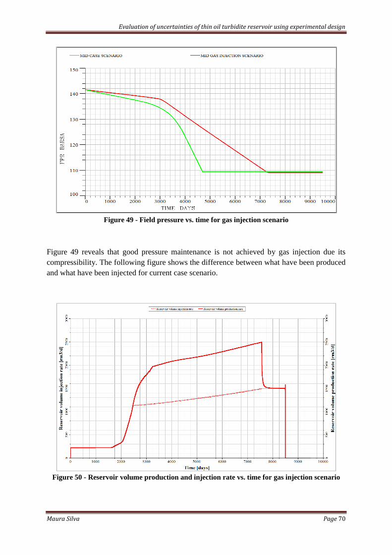
Evaluation of uncertainties of thin oil turbidite reservoir using experimental design
Maura Silva Page 70
Figure 49 - Field pressure vs. time for gas injection scenario
Figure 49 reveals that good pressure maintenance is not achieved by gas injection due its
compressibility. The following figure shows the difference between what have been produced
and what have been injected for current case scenario.
Figure 50 - Reservoir volume production and injection rate vs. time for gas injection scenario
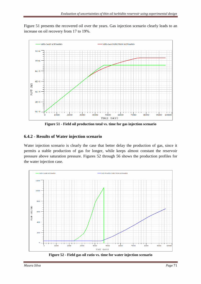
Evaluation of uncertainties of thin oil turbidite reservoir using experimental design
Maura Silva Page 71
Figure 51 presents the recovered oil over the years. Gas injection scenario clearly leads to an
increase on oil recovery from 17 to 19%.
Figure 51 - Field oil production total vs. time for gas injection scenario
6.4.2 - Results of Water injection scenario
Water injection scenario is clearly the case that better delay the production of gas, since it
permits a stable production of gas for longer, while keeps almost constant the reservoir
pressure above saturation pressure. Figures 52 through 56 shows the production profiles for
the water injection case.
Figure 52 - Field gas oil ratio vs. time for water injection scenario

Evaluation of uncertainties of thin oil turbidite reservoir using experimental design
Maura Silva Page 72
Figure 53 - Field water cut vs. time for water injection scenario
As observed on fig. 54 it is well seen how the pressure in being maintained at early stages of
production as stated on control mode. It is verified that the desired pressure maintenance as
stated on control mode was not achieved so, an increase on water injection rate could be
considered.
Figure 54 - Field pressure vs. time for water injection scenario
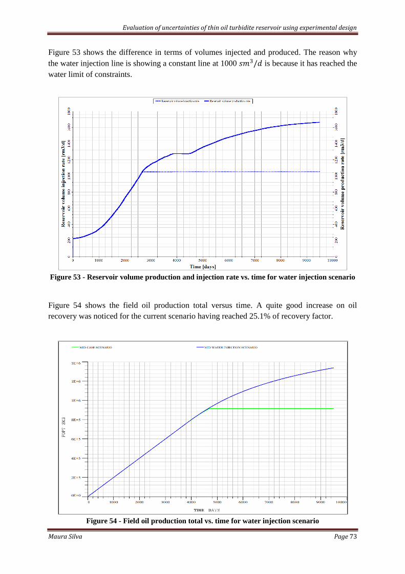
Evaluation of uncertainties of thin oil turbidite reservoir using experimental design
Maura Silva Page 73
Figure 53 shows the difference in terms of volumes injected and produced. The reason why
the water injection line is showing a constant line at 1000 is because it has reached the
water limit of constraints.
Figure 53 - Reservoir volume production and injection rate vs. time for water injection scenario
Figure 54 shows the field oil production total versus time. A quite good increase on oil
recovery was noticed for the current scenario having reached 25.1% of recovery factor.
Figure 54 - Field oil production total vs. time for water injection scenario
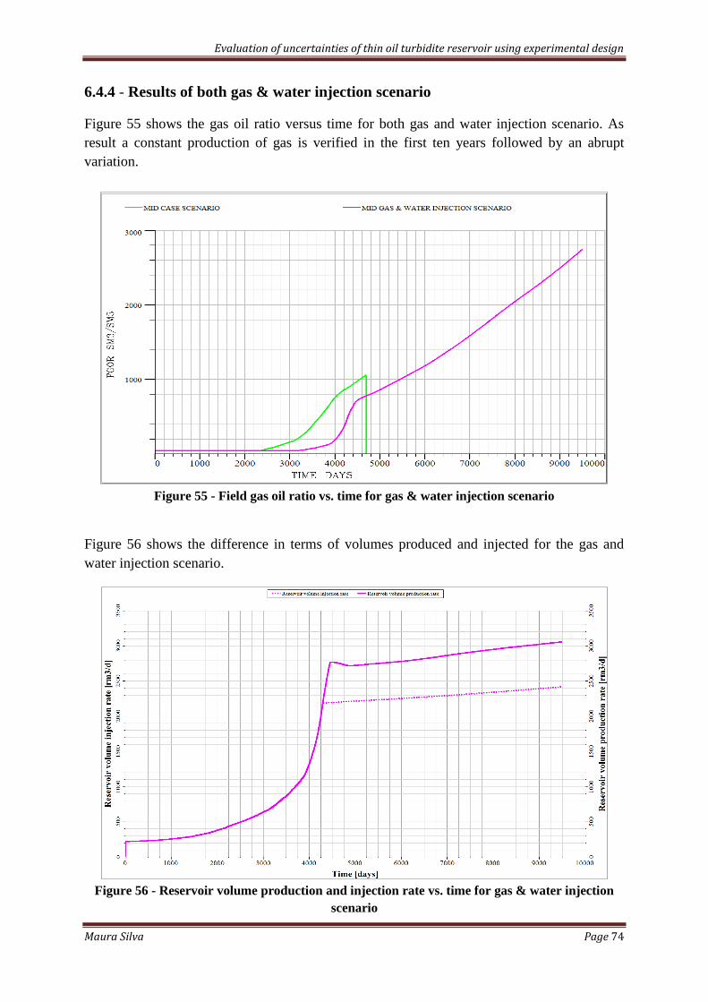
Evaluation of uncertainties of thin oil turbidite reservoir using experimental design
Maura Silva Page 74
6.4.4 - Results of both gas & water injection scenario
Figure 55 shows the gas oil ratio versus time for both gas and water injection scenario. As
result a constant production of gas is verified in the first ten years followed by an abrupt
variation.
Figure 55 - Field gas oil ratio vs. time for gas & water injection scenario
Figure 56 shows the difference in terms of volumes produced and injected for the gas and
water injection scenario.
Figure 56 - Reservoir volume production and injection rate vs. time for gas & water injection
scenario
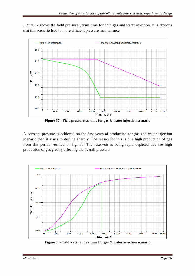
Evaluation of uncertainties of thin oil turbidite reservoir using experimental design
Maura Silva Page 75
Figure 57 shows the field pressure versus time for both gas and water injection. It is obvious
that this scenario lead to more efficient pressure maintenance.
Figure 57 - Field pressure vs. time for gas & water injection scenario
A constant pressure is achieved on the first years of production for gas and water injection
scenario then it starts to decline sharply. The reason for this is due high production of gas
from this period verified on fig. 55. The reservoir is being rapid depleted due the high
production of gas greatly affecting the overall pressure.
Figure 58 - field water cut vs. time for gas & water injection scenario
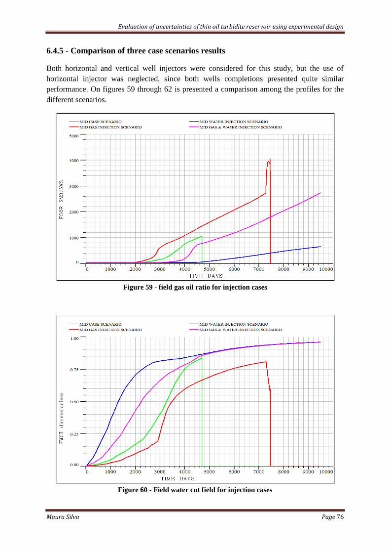
Evaluation of uncertainties of thin oil turbidite reservoir using experimental design
Maura Silva Page 76
6.4.5 - Comparison of three case scenarios results
Both horizontal and vertical well injectors were considered for this study, but the use of
horizontal injector was neglected, since both wells completions presented quite similar
performance. On figures 59 through 62 is presented a comparison among the profiles for the
different scenarios.
Figure 59 - field gas oil ratio for injection cases
Figure 60 - Field water cut field for injection cases
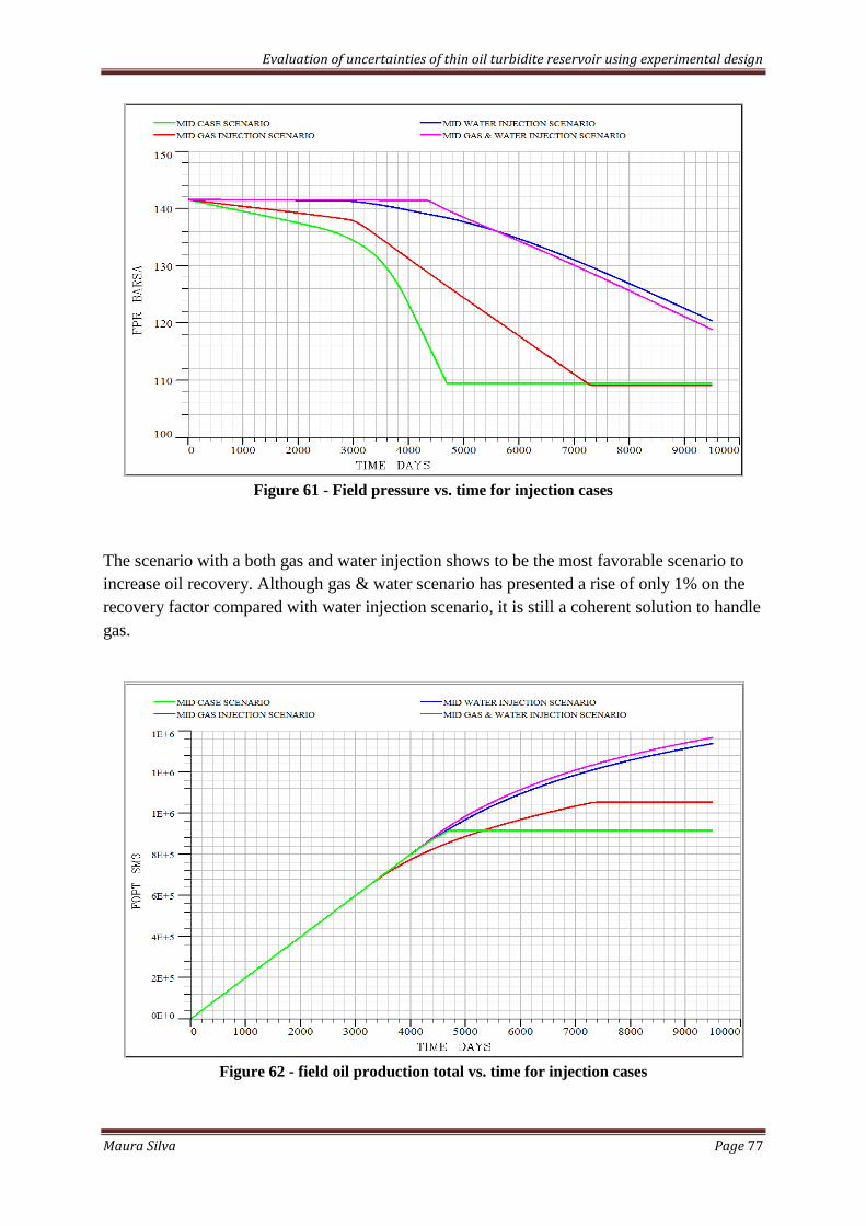
Evaluation of uncertainties of thin oil turbidite reservoir using experimental design
Maura Silva Page 77
Figure 61 - Field pressure vs. time for injection cases
The scenario with a both gas and water injection shows to be the most favorable scenario to
increase oil recovery. Although gas & water scenario has presented a rise of only 1% on the
recovery factor compared with water injection scenario, it is still a coherent solution to handle
gas.
Figure 62 - field oil production total vs. time for injection cases
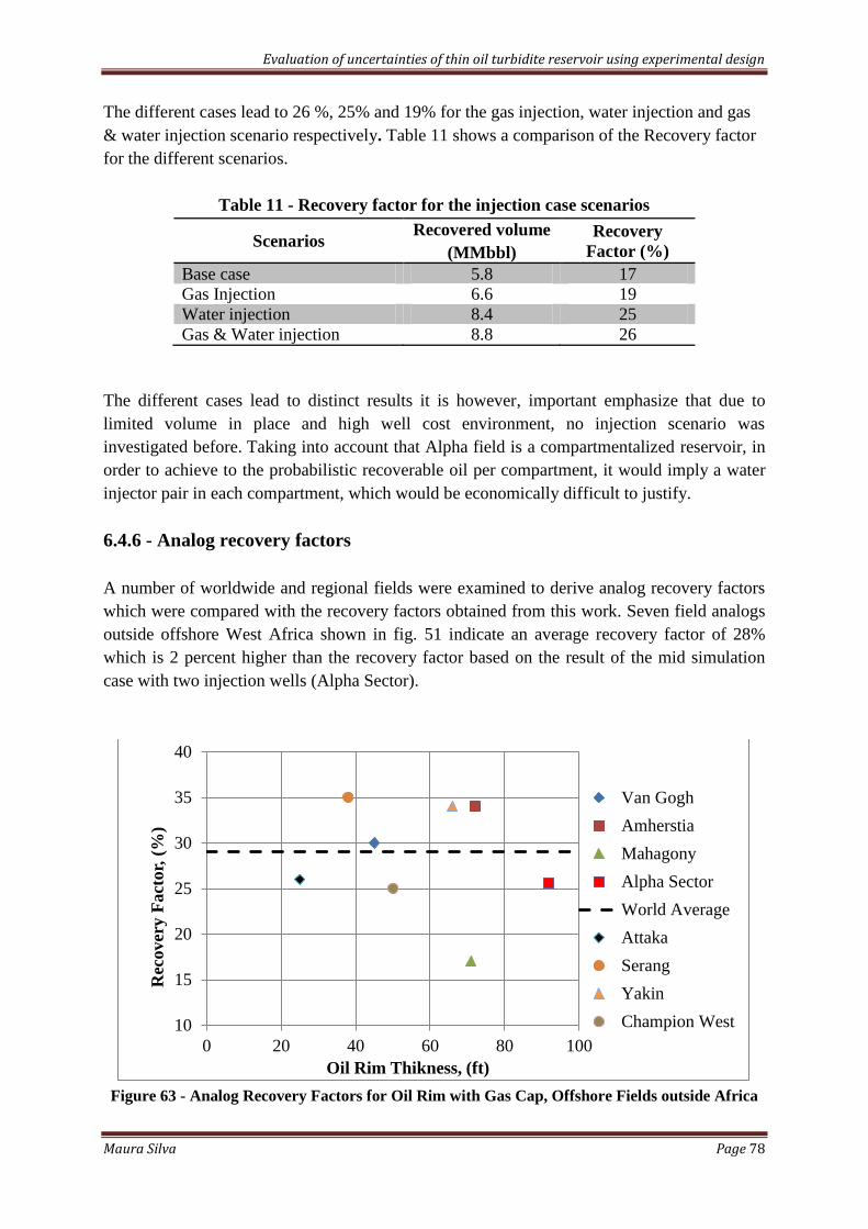
Evaluation of uncertainties of thin oil turbidite reservoir using experimental design
Maura Silva Page 78
The different cases lead to 26 %, 25% and 19% for the gas injection, water injection and gas
& water injection scenario respectively. Table 11 shows a comparison of the Recovery factor
for the different scenarios.
Table 11 - Recovery factor for the injection case scenarios
Scenarios Recovered volume
(MMbbl)
Recovery
Factor (%)
Base case 5.8 17
Gas Injection 6.6 19
Water injection 8.4 25
Gas & Water injection 8.8 26
The different cases lead to distinct results it is however, important emphasize that due to
limited volume in place and high well cost environment, no injection scenario was
investigated before. Taking into account that Alpha field is a compartmentalized reservoir, in
order to achieve to the probabilistic recoverable oil per compartment, it would imply a water
injector pair in each compartment, which would be economically difficult to justify.
6.4.6 - Analog recovery factors
A number of worldwide and regional fields were examined to derive analog recovery factors
which were compared with the recovery factors obtained from this work. Seven field analogs
outside offshore West Africa shown in fig. 51 indicate an average recovery factor of 28%
which is 2 percent higher than the recovery factor based on the result of the mid simulation
case with two injection wells (Alpha Sector).
Figure 63 - Analog Recovery Factors for Oil Rim with Gas Cap, Offshore Fields outside Africa
10
15
20
25
30
35
40
0 20 40 60 80 100
Rec
over
y F
act
or,
(%
)
Oil Rim Thikness, (ft)
Van Gogh
Amherstia
Mahagony
Alpha Sector
World Average
Attaka
Serang
Yakin
Champion West

Evaluation of uncertainties of thin oil turbidite reservoir using experimental design
Maura Silva Page 79
CHAPTER VII – CONCLUSION
The main goal of this thesis was to evaluate the uncertainties of a thin oil reservoir discovery
using experimental design. The reservoir consists of various channels, which divide it into
several compartments with different heterogeneity and fluids oil contacts. A secondary
objective was relate with coning study, where the main objective was to estimate the critical
oil production rate through analytical correlations and numerical simulation, using available
reservoir modeling tools. A development scheme with water and gas injection was also
investigated. Based on the results the following general conclusions were achieved.
Increasing grid resolution improves the coning interpretation and provides good accuracy on
results but the process can be very time consuming. Therefore, a good compromise between
computational time and accuracy of results was achieved.
Due to the conflicting results of analytical correlations they should be carefully used when
implemented in a specific field data and further investigations (i.e. model simulations) should
be considered in order to support the results.
The adopted screening design shows relative permeability, horizontal permeability and Rock
compressibility as the key uncertainties parameters. The study clearly suggests that SCAL
data are required. Indicating that the data availability to be really important in provide
confident results and therefore a more realistic plan would be achieved.
Pressure maintenance is required to maximize oil recovery. The development scheme scenario
with a both gas and water injection shows to be the most favorable scenario with 26% of oil
recovered. Although gas and water scenario has presented a slightly rise on the recovery
factor compared with water injection scenario, it is still a coherent solution to handle gas.

Evaluation of uncertainties of thin oil turbidite reservoir using experimental design
Maura Silva Page 80
RECOMMENDATIONS FOR FURTHER WORK
• Well modelization (Inflow/outflow, to understand the regime of fluid transportation
inside the tubing).
• Impact on three phase relative permeability (to get more accurate knowledge of fluid
movement in the analyses).
• Integration with surface engineering
Development concept and facility capacity constraints
Flow assurance
• Sensitivity on injection wells (varying distances between the wells should be
investigated to determine any effect on well spacing)

Evaluation of uncertainties of thin oil turbidite reservoir using experimental design
Maura Silva Page 81
REFERENCE
Alpha 2011. Internal Maersk oil Integrated Field Study report Alpha 2011.
ASQC, 1983. Glossary & Tables for Statistical Quality Control.
http://books.google.dk/books/about/Glossary_and_tables_for_statistical_qual.html?id=LsFTA
AAAMAAJ&redir_esc=y - 2014/05/30.
Begg, S., Bratvold, R.B. and Campbell, J.M., 2001. Improving Investment Decisions Using a
Friedmann, F., Chawathe, A. and Larue, D.K., 2003. Assessing Uncertainty in Channelized
Reservoirs Using Experimental Designs, SPE 85117 revised for publication from paper SPE
71622, first presented at the 2001 SPE Annual Tachnical Conference and Exhibition, New
Orlenans, from 30th
of September to 3rd
of October. Paper peer approved on 22nd
May of
2003.
Gawish A., 2007. Visual basic program for study water and gas parameters.
Giger F. M., 1986. Analytic 2-D Models Of Water Cresting Before Breakthrough for
Horizontal Wells. Paper SPE 15378 presented at the 61st SPE Annual Technical Conference
and Exhibition, New Orleans (LA), 5-8 October.
Guo B., Molinard J. E., France G. D. and Lee R.L., 1992. A General Solution of Gas/Water
Coning Problem for Horizontal Well. SPE 25050 paper prepared for presentation at the
European Petroleum Conference held in Cannes - France from 16th
to 18th
of November.
Itotoi I. H., Ojeke A. And Nnamdi D., 2010. Managing reservoir uncertainty in gas field
development using experimental design. Paper SPE 140619 prepared for presentation at 34th
Annual SPE International Conference and Exhibition held in, Tinapa – Calabar, Nigeria 31
July – 7 August.
Joshi S.D., “Augmentation of Well Productivity Using Slant and Horizontal Wells”, JPT No.6,
June 1988, pp. 729-739.
Joshi S.D., “Horizontal well technology”, Pennwell Publishing Company, 1991, pp. 535.
Kazeem A. Lawal, Ademola O. Adenuga, 2010. Preliminary Assessment of Oil-Rim
reservoirs: A review of current practices and formulation of new concepts. SPE 136955 paper
prepared for the 34th
Annual SPE International Conference and Exibition held in Tinapa.
Calabar, Nigeria 31st July to 7
th August.
Khalili A., 2005. A review of critical coning rate correlations and identifying the most
reliable equation. Submitted to the School of Petroleum Engineering of University of New
south Wales in partial fulfillment of the requirements for the degree of master of engineering.
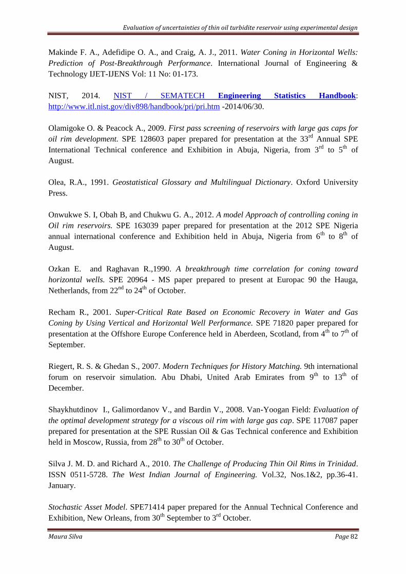
Evaluation of uncertainties of thin oil turbidite reservoir using experimental design
Maura Silva Page 82
Makinde F. A., Adefidipe O. A., and Craig, A. J., 2011. Water Coning in Horizontal Wells:
Prediction of Post-Breakthrough Performance. International Journal of Engineering &
Technology IJET-IJENS Vol: 11 No: 01-173.
NIST, 2014. NIST / SEMATECH Engineering Statistics Handbook:
http://www.itl.nist.gov/div898/handbook/pri/pri.htm -2014/06/30.
Olamigoke O. & Peacock A., 2009. First pass screening of reservoirs with large gas caps for
oil rim development. SPE 128603 paper prepared for presentation at the 33rd
Annual SPE
International Technical conference and Exhibition in Abuja, Nigeria, from 3rd
to 5th
of
August.
Olea, R.A., 1991. Geostatistical Glossary and Multilingual Dictionary. Oxford University
Press.
Onwukwe S. I, Obah B, and Chukwu G. A., 2012. A model Approach of controlling coning in
Oil rim reservoirs. SPE 163039 paper prepared for presentation at the 2012 SPE Nigeria
annual international conference and Exhibition held in Abuja, Nigeria from 6th
to 8th
of
August.
Ozkan E. and Raghavan R.,1990. A breakthrough time correlation for coning toward
horizontal wells. SPE 20964 - MS paper prepared to present at Europac 90 the Hauga,
Netherlands, from 22nd
to 24th
of October.
Recham R., 2001. Super-Critical Rate Based on Economic Recovery in Water and Gas
Coning by Using Vertical and Horizontal Well Performance. SPE 71820 paper prepared for
presentation at the Offshore Europe Conference held in Aberdeen, Scotland, from 4th
to 7th
of
September.
Riegert, R. S. & Ghedan S., 2007. Modern Techniques for History Matching. 9th international
forum on reservoir simulation. Abu Dhabi, United Arab Emirates from 9th
to 13th
of
December.
Shaykhutdinov I., Galimordanov V., and Bardin V., 2008. Van-Yoogan Field: Evaluation of
the optimal development strategy for a viscous oil rim with large gas cap. SPE 117087 paper
prepared for presentation at the SPE Russian Oil & Gas Technical conference and Exhibition
held in Moscow, Russia, from 28th
to 30th
of October.
Silva J. M. D. and Richard A., 2010. The Challenge of Producing Thin Oil Rims in Trinidad.
ISSN 0511-5728. The West Indian Journal of Engineering. Vol.32, Nos.1&2, pp.36-41.
January.
Stochastic Asset Model. SPE71414 paper prepared for the Annual Technical Conference and
Exhibition, New Orleans, from 30th
September to 3rd
October.

Evaluation of uncertainties of thin oil turbidite reservoir using experimental design
Maura Silva Page 83
Verga F, Viberti D., Ferraro P., and Torino P. D., 2007. Prediction of water coning and water
cresting: analytical or numerical models. OMC 2007-173 paper presented at the Offshore
Mediterranean Conference and Exhibition in Ravenna, Italy, from 28th
to 30th
of March.
Veskimägi V., 2013. Gas Coning Control with a Smart Horizontal Well in a Thin Oil Rim.
TA Report number AES/PE/13-09. Section for Petroleum Engineering Department of
Geoscience & Engineering.
Walstrom, J.E. & Mueller, T.D., McFarlane, R.C., 1967. Evaluating Uncertainty in
Engineering Calculations. Journal of Petroleum Technology, Dec 1967, pag 1595 - 1603 .
Paper SPE 1928presented at SPE 42nd Annual Fall Meeting held in Houston, Tex. From 1st
to 4th
of Octuber.
Yang W. & Wattenbarger R. A., 1991. Water coning calculations for vertical and horizontal
wells. SPE 22931 paper prepared for presentation at the 66th
Annual conference and
exhibition of the society of petroleum engineers held in Dallas, TX, from 6th
to 9th
of October.
Yeten B., Castellini A., Guyaguler B., and Chen W. H., 2005. A comparison study on
Experimental Design and response surface methodologies. Paper SPE 93347 prepared for
presentation at the 2005 SPE Reservoir Simulatiuon Symposium held in, Houston, Texas -
U.S.A from 31st
of January to 2nd
of February.
Zakirov S. N., and Zakirov I. S., 1996. New Methods for Improved Oil Recovey of Thin Oil
Rim. SPE 36845paper prepared for presentation at the SPE European Petroleum Conference
held in Milan, Italy, from 22nd
to 24th
of October.

Evaluation of uncertainties of thin oil turbidite reservoir using experimental design
Maura Silva Page 84
APPENDICES
Figure 64 - critical oil correlation on VBA

Evaluation of uncertainties of thin oil turbidite reservoir using experimental design
Maura Silva Page 85
Figure 65 - Defining variables to generate the design matrix on Petrel
Figure 66 - Selecting method and and generating matrix design
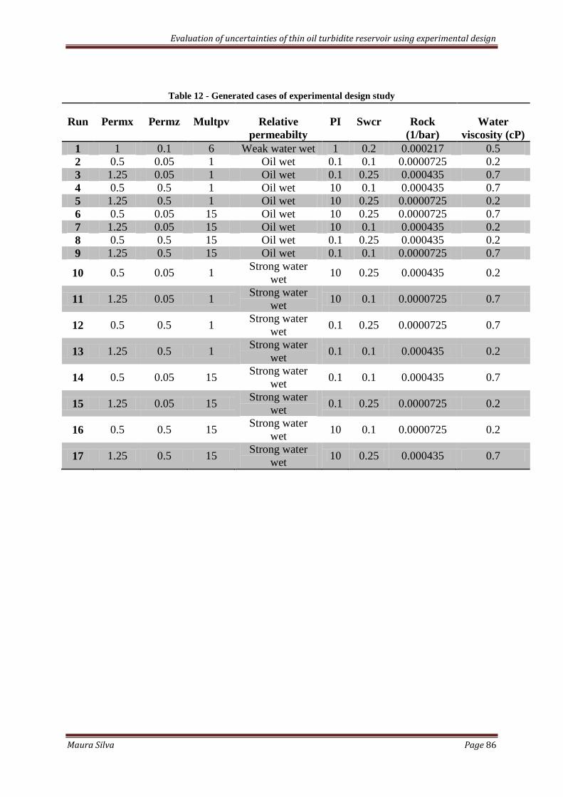
Evaluation of uncertainties of thin oil turbidite reservoir using experimental design
Maura Silva Page 86
Table 12 - Generated cases of experimental design study
Run Permx Permz Multpv Relative
permeabilty
PI Swcr Rock
(1/bar)
Water
viscosity (cP)
1 1 0.1 6 Weak water wet 1 0.2 0.000217 0.5
2 0.5 0.05 1 Oil wet 0.1 0.1 0.0000725 0.2
3 1.25 0.05 1 Oil wet 0.1 0.25 0.000435 0.7
4 0.5 0.5 1 Oil wet 10 0.1 0.000435 0.7
5 1.25 0.5 1 Oil wet 10 0.25 0.0000725 0.2
6 0.5 0.05 15 Oil wet 10 0.25 0.0000725 0.7
7 1.25 0.05 15 Oil wet 10 0.1 0.000435 0.2
8 0.5 0.5 15 Oil wet 0.1 0.25 0.000435 0.2
9 1.25 0.5 15 Oil wet 0.1 0.1 0.0000725 0.7
10 0.5 0.05 1 Strong water
wet 10 0.25 0.000435 0.2
11 1.25 0.05 1 Strong water
wet 10 0.1 0.0000725 0.7
12 0.5 0.5 1 Strong water
wet 0.1 0.25 0.0000725 0.7
13 1.25 0.5 1 Strong water
wet 0.1 0.1 0.000435 0.2
14 0.5 0.05 15 Strong water
wet 0.1 0.1 0.000435 0.7
15 1.25 0.05 15 Strong water
wet 0.1 0.25 0.0000725 0.2
16 0.5 0.5 15 Strong water
wet 10 0.1 0.0000725 0.2
17 1.25 0.5 15 Strong water
wet 10 0.25 0.000435 0.7
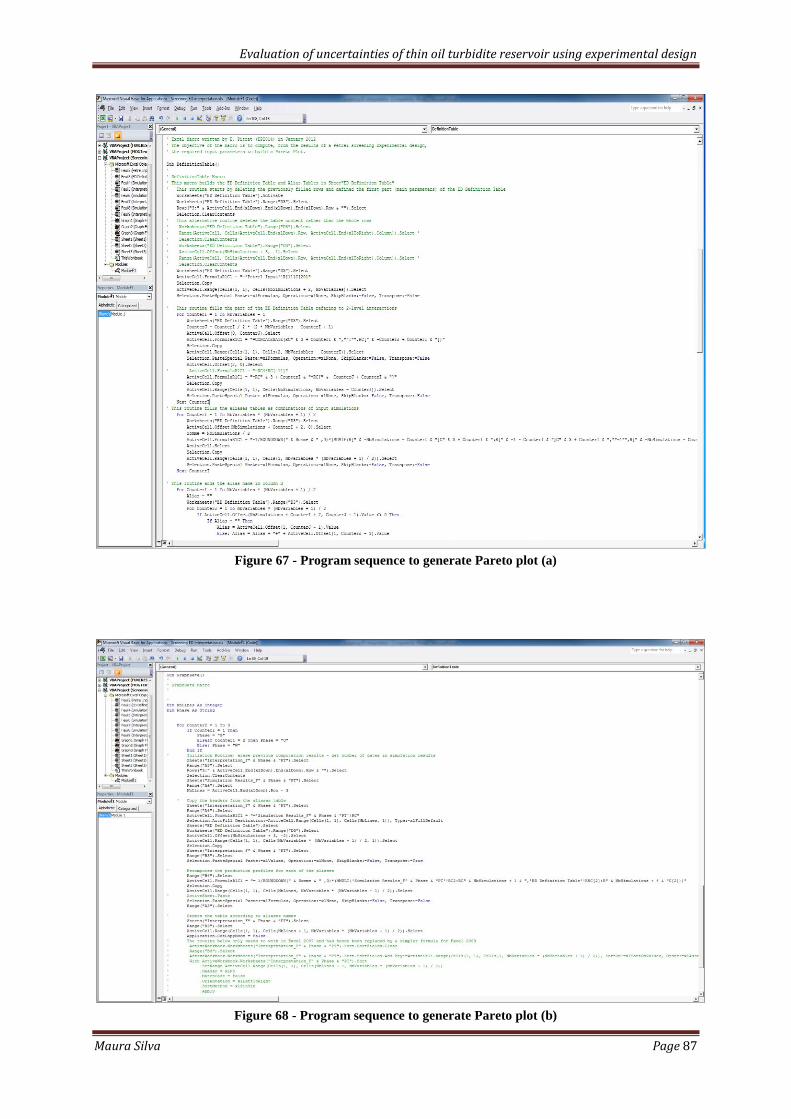
Evaluation of uncertainties of thin oil turbidite reservoir using experimental design
Maura Silva Page 87
Figure 67 - Program sequence to generate Pareto plot (a)
Figure 68 - Program sequence to generate Pareto plot (b)

Evaluation of uncertainties of thin oil turbidite reservoir using experimental design
Maura Silva Page 88
Figure 6969 - Gas production cumulative vs. time of the ED cases
Figure 70 - Gas production rate vs. time of the ED cases
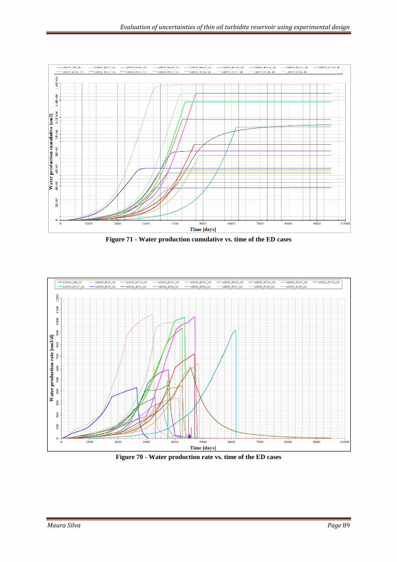
Evaluation of uncertainties of thin oil turbidite reservoir using experimental design
Maura Silva Page 89
Figure 71 - Water production cumulative vs. time of the ED cases
Figure 70 - Water production rate vs. time of the ED cases
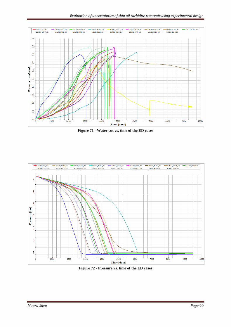
Evaluation of uncertainties of thin oil turbidite reservoir using experimental design
Maura Silva Page 90
Figure 71 - Water cut vs. time of the ED cases
Figure 72 - Pressure vs. time of the ED cases

Evaluation of uncertainties of thin oil turbidite reservoir using experimental design
Maura Silva Page 91
Figure 73 - CPU time vs. time of the ED cases
Figure 74 - Gas production cumulative and oil production rate vs. time of the three main ED cases
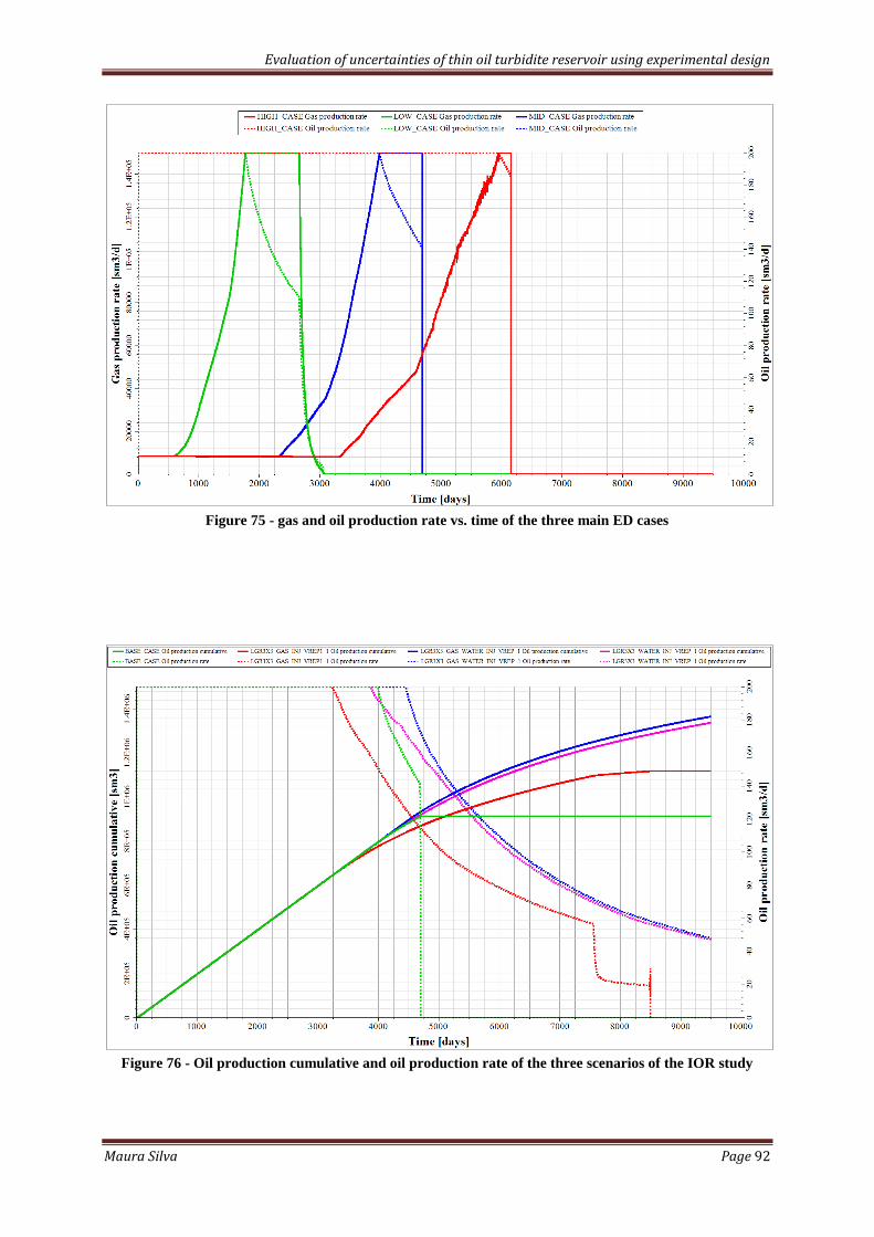
Evaluation of uncertainties of thin oil turbidite reservoir using experimental design
Maura Silva Page 92
Figure 75 - gas and oil production rate vs. time of the three main ED cases
Figure 76 - Oil production cumulative and oil production rate of the three scenarios of the IOR study
Copyright © 2022 FDOKUMEN