CO : CO2, N2O : CO2, CH4 : CO2, O2 : CO2 ratios - ACP ...

Atmos. Chem. Phys., 14, 2105–2123, 2014www.atmos-chem-phys.net/14/2105/2014/doi:10.5194/acp-14-2105-2014© Author(s) 2014. CC Attribution 3.0 License.

Atmospheric Chemistry

and PhysicsO

pen Access

Vehicle emissions of greenhouse gases and related tracers from atunnel study: CO : CO2, N2O : CO2, CH4 : CO2, O2 : CO2 ratios, andthe stable isotopes13C and 18O in CO2 and CO

M. E. Popa1, M. K. Vollmer 2, A. Jordan3, W. A. Brand3, S. L. Pathirana1, M. Rothe3, and T. Röckmann1

1Institute for Marine and Atmospheric research Utrecht, Utrecht University, Princetonplein 5, 3508TA Utrecht, theNetherlands2Empa, Swiss Federal Laboratories for Materials Testing and Research, Laboratory for Air Pollution and EnvironmentalTechnology, Überlandstrasse 129, 8600 Dübendorf, Switzerland3Max-Planck Institute for Biogeochemistry, Hans-Knöll-Str. 10, 07745 Jena, Germany

Correspondence to:M. E. Popa ([email protected])

Received: 7 August 2013 – Published in Atmos. Chem. Phys. Discuss.: 6 September 2013Revised: 13 December 2013 – Accepted: 16 December 2013 – Published: 24 February 2014

Abstract. Measurements of CO2, CO, N2O and CH4 molefractions, O2 / N2 ratios and the stable isotopes13C and18O in CO2 and CO have been performed in air samplesfrom the Islisberg highway tunnel (Switzerland). The molarCO : CO2 ratios, with an average of (4.15± 0.34) ppb:ppm,are lower than reported in previous studies, pointing to a re-duction in CO emissions from traffic. The13C in CO2 re-flects the isotopic composition of the fuel.18O in CO2 isslightly depleted compared to the18O in atmospheric O2,and shows significant variability. In contrast, theδ13C val-ues of CO show that significant fractionation takes placeduring CO destruction in the catalytic converter.13C in COis enriched by 3 ‰ compared to the13C in the fuel burnt,while the18O content is similar to that of atmospheric O2.We compute a fractionation constant of (−2.7± 0.7) ‰ for13C during CO destruction. The N2O : CO2 average ratioof (1.8± 0.2)× 10−2 ppb:ppm is significantly lower than inpast studies, showing a reduction in N2O emissions likelyrelated to improvements in the catalytic converter technol-ogy. We also observed small CH4 emissions, with an av-erage CH4 : CO2 ratio of (4.6± 0.2)× 10−2 ppb:ppm. TheO2 : CO2 ratios of (−1.47± 0.01) ppm:ppm are very close tothe expected, theoretically calculated values of O2 depletionper CO2 enhancement.

1 Introduction

In densely populated areas, traffic emissions are a significantsource of trace gases and pollutants. The main product of fuelburning is CO2, but a wide series of other gases are emittedconcurrently. Some of these are short lived and have mainlylocal health and environmental effects. Long lived gases, likeCO2, CH4, N2O, CO, and H2, are (indirect) greenhouse gasesand have global effects on atmospheric chemistry and cli-mate.

CO2 emissions from traffic can be computed fairly ac-curately from fuel consumption statistics. The emissions ofother gases are more difficult to estimate and depend stronglyon technology, vehicle type and driving conditions. The in-troduction of catalytic converters led to a strong decrease inthe emissions of some gases, and emissions further decreasedwith each generation of emission standards. In Europe for ex-ample, the accepted CO emission for Euro 3 passenger gaso-line vehicles was 2.3 g km−1, and the Euro 4 and Euro 5 stan-dards decreased the limit to 1 g km−1. Other relevant gases,like for example H2 and N2O, are not controlled by the ex-isting vehicle emission standards, while CH4 is usually onlyincluded in the total hydrocarbon category. However, vehi-cle emissions of N2O and CH4 have to be estimated and in-cluded in annual reports by the United Nations FrameworkConvention on Climate Change (UNFCCC) partners. Theseestimations are based on traffic statistics and emission factors

Published by Copernicus Publications on behalf of the European Geosciences Union.

2106 M. E. Popa et al.: Vehicle emissions of greenhouse gases

(IPCC, 1997; UNFCCC, 2006), thus it is important that emis-sion factors reflect the actual real-life emissions.

Because of the relatively fast evolution of vehicle technol-ogy and emission standards, emissions can change signifi-cantly on timescales of several years. Besides this, differentcomposition and age of the car fleet lead to large regionaldifferences in emissions.

Vehicle emission rates (or factors) are used together withtraffic statistics to estimate traffic emissions at various scales.Emission rates are often obtained in laboratory setup by dy-namometer studies, but it has been shown that the results donot always represent the real-life emissions (Ropkins et al.,2009 and references therein). Tunnel measurements provedto be very useful for estimating real-world fleet-wide emis-sion rates (see Ropkins et al., 2009 for a review of emis-sion estimation methods). The obvious advantage of a tun-nel setup is that it allows observing real-life traffic emis-sions while keeping out other possible sources. Tunnel stud-ies have, however, some limitations; for example, they aremostly representative for fluent traffic conditions and not forurban driving with frequent stops and accelerations. Thustunnel measurements have to be complemented by othertypes of measurements in order to obtain a complete picture.

The Islisberg-2011 measurement campaign took place inJune–July 2011 at the Islisberg highway tunnel located nearZürich, Switzerland, with the intention to update (whereolder estimates exist) or quantify emissions and isotopic sig-natures of several important long lived trace gases, character-istic to the western European vehicle fleet.

The purpose of the present paper is as follows:

– to quantify CO : CO2, N2O : CO2 and CH4 : CO2 emis-sion ratios for the present vehicle fleet;

– to determine the present isotopic signatures of traffic-emitted CO2 and CO;

– to verify the theoretically calculated O2 : CO2 ratios oftraffic emissions.

Results on the H2 : CO emission ratios and H2 isotopic sig-natures will be presented in a different publication.

The remainder of the paper is organized as follows. Sec-tion 1.1 contains background information on each speciesdealt with in the paper – we considered necessary to in-clude this information, but it can be skipped by the expertreader. Section 2 presents the sampling and measurementmethods. Section 3 starts with a general description of thedata acquired and continues with a detailed discussion onthe CO : CO2 ratios and the isotopic composition of CO2 andCO, followed by N2O : CO2, CH4 : CO2 and O2 : CO2 ratios.Section 4 contains a summary of our findings. The Supple-ment includes a more detailed description of the CO molefraction measurements at the Institute for Marine and At-mospheric research Utrecht (IMAU) and the main numericaldata used in the paper.

1.1 Background on the investigated species

CO : CO2 ratios

CO is an atmospheric trace gas that results from incompleteoxidation of carbon. Anthropogenic emissions are responsi-ble for a large part of the global CO; in Europe anthropogenicsources account for about 70 % of the total sources (Pfister etal., 2004). About a quarter of these emissions were in 2010from road transport (EEA, 2013).

CO is important for the atmospheric chemistry, mainly dueto its reaction with OH radicals. CO is also a toxic gas and,because some of its largest sources are associated with hu-man agglomerations, it is a concern for human (and animal)health. Thus most urban air quality monitoring programs in-clude CO. Besides these, CO is a good tracer for detectingand quantifying anthropogenic emissions from burning pro-cesses, since it is a product of incomplete burning. For ex-ample, the ratio between atmospheric variations of CO andCO2 (the CO : CO2 ratio) has been used to quantify the fossilfuel contribution to the CO2 variability and the CO2 fossilfuel fluxes (e.g. Gamnitzer et al., 2006; Levin and Karstens,2007; Rivier et al., 2006; Turnbull et al., 2006, 2011; Zon-dervan and Meijer, 1996). The CO : CO2 ratios are higher forpoorer burning (e.g. forest fires), thus these ratios can be usedto distinguish between different burning processes or to de-termine the burning efficiency (Andreae and Merlet, 2001;Röckmann et al., 2010; Suntharalingam et al., 2004; Wang etal., 2010).

Anthropogenic emissions of CO have been decreasingover the last two decades, according to various inventories(see e.g. Granier et al., 2011), and the decrease in emissionsis reflected in decreasing atmospheric mole fractions in ur-ban areas, background areas and in the atmospheric column(Angelbratt et al., 2011; von Schneidemesser et al., 2010;Worden et al., 2013; Zellweger et al., 2009); for Europe, thedecreasing trends are larger than the global ones.

In populated regions like Europe one of the major sourcesof CO2 and CO is road traffic. The CO2 emission rate is rel-atively constant, as it depends directly on the quantity of fuelburnt. Emissions of CO, on the other hand, are strongly de-pendent on vehicle technology and thus on fleet composition.Emission standards gradually lowered the limits of allowedCO from Euro 1 to Euro 4. A gradual decrease in emis-sions from pre-Euro to Euro 4 cars has been confirmed byreal-world measurements (e.g. Rhys-Tyler et al., 2011). Thestricter vehicle emission standards and the mandatory intro-duction of catalytic converters in new cars at the beginningof the 1990s are partly responsible for the decrease in emis-sions.

It is expected that traffic CO emissions will continue todecrease while older vehicles are replaced by new ones. Itis also likely that the overall anthropogenic emissions ofCO in Europe (and in consequence the CO : CO2 ratios)will continue to decrease with the evolution towards cleaner

Atmos. Chem. Phys., 14, 2105–2123, 2014 www.atmos-chem-phys.net/14/2105/2014/

M. E. Popa et al.: Vehicle emissions of greenhouse gases 2107

technologies, under the pressure of pollution reduction poli-cies. Periodically updating the information on CO : CO2emission ratios for different sources will reduce uncertain-ties in CO emission inventories. This will on one hand im-prove the possibility to use these ratios for CO2 source dis-crimination. On the other hand, for vehicle emissions, whereCO2 is relatively well known from fuel consumption, knownCO : CO2 ratios can help determining CO emissions, whichis important for example for assessment and control of pol-lution in populated areas.

1.1.1 CO2 stable isotopes13C and 18O

Numerous studies have used the isotopic composition of at-mospheric CO2 in order to constrain various aspects of thecarbon cycle (e.g. Battle et al., 2000; Gruber and Keeling,2001; Yakir and Sternberg, 2000; Yakir and Wang, 1996).In general, the isotopic composition of atmospheric CO2 islinked to the biosphere–atmosphere exchange and, in the caseof 18O, to the water cycle (Farquhar et al., 1993; Franceyand Tans, 1987; Mills and Urey, 1940). However, especiallyin highly populated areas like Europe, a significant part ofthe CO2 emitted originates from fossil fuel burning. Goodknowledge on the isotopic composition of the fossil fuel-derived CO2 can in principle help interpreting atmosphericmeasurements and partitioning sources and sinks at local andregional level (e.g. Meijer et al., 1996; Pataki et al., 2003,2006, 2007; Zimnoch et al., 2004; Zondervan and Meijer,1996).

In modelling studies so far, the18O isotopic ratio ofcombustion-derived CO2 is considered to be equal to the18O isotopic ratio of atmospheric O2 (e.g. Ciais et al., 1997;Cuntz et al., 2003). This assumes that atmospheric O2 is con-sumed without fractionation; however, this has been ques-tioned by some recent studies. For example, Affek and Eiler(2006), Horvath et al. (2012) and Schumacher et al. (2011)found the18O in vehicle exhaust CO2 to be significantly dif-ferent from the18O in atmospheric O2; combustion of othermaterials has been shown to suffer fractionation processesaffecting18O in CO2 as well. More work appears thus neces-sary for better defining the source signatures of CO2 resultingfrom different burning processes.

1.1.2 CO stable isotopes13C and 18O

Stable isotopes have been used as a tool to distinguish be-tween CO emission sources, for example to distinguish be-tween traffic and wood combustion (Saurer et al., 2009), toidentify large scale pollution from forest fires (Röckmann etal., 2002) and to identify various anthropogenic emissions(e.g. Tarasova et al., 2007). Also, modelling studies that in-cluded13C and18O provided more robust results than whenconsidering CO mole fractions alone (Bergamaschi et al.,2000; Manning et al., 1997). For these uses, however, thesource-specific isotopic signatures have to be known. It has

been shown that the13C and18O isotopic signatures of COfrom combustion sources are not necessarily the same as the13C of the material burnt and the18O in the atmospheric O2due to fractionation during the burning process (e.g. Kato etal., 1999a, b; Tsunogai et al., 2003). Relatively few estimatesexist on the isotopic signatures of different CO sources, andin particular on traffic CO, although in some areas trafficemissions account for a large proportion of anthropogenicCO sources.

There are two main types of studies regarding the isotopiccomposition of CO emitted by traffic, which are complemen-tary. One consists of fleet integrated measurements, with re-sults representative for the real-world average traffic emis-sions. Only few such studies exist worldwide (Kato et al.,1999a; Stevens et al., 1972; Tsunogai et al., 2003); the mostrecent measurements in Europe were performed in 1997 byKato et al. (1999a).

The other category of studies focuses on measuringemissions of individual vehicles or engines (e.g. Huff andThiemens, 1998; Kato et al., 1999a; Tsunogai et al., 2003);upscaling their results to fleet level is not always straightfor-ward, but these studies are particularly useful for understand-ing the factors controlling the emissions and the phenomenabehind. As revealed by the studies above, the isotopic com-position of exhaust CO is strongly dependent on vehicle tech-nology. 13C in CO in exhaust gas is approximately similarto that in the fuel for old vehicles without a catalyst, and itis enriched for gasoline vehicles with catalyst and for dieselvehicles.18O is enriched relative to atmospheric O2 for gaso-line vehicles with catalyst, and is depleted for old gasolinevehicles without catalyst and for diesel vehicles. The driv-ing regime and the temperature of the catalyst have been ob-served to affect the isotopic composition of emitted CO aswell.

The above implies that the isotopic composition of trafficCO should change in time with the change in technology, in-creasing proportion of vehicles equipped with catalytic con-verters, and changing shares for different fuel types. Suchevolution is already clear when comparing the results of oldand new estimates, and it is expected that the CO isotopiccomposition will continue to change and will have to be re-evaluated periodically (Tsunogai et al., 2003).

1.1.3 N2O : CO2 ratios

N2O is an important greenhouse gas, considered to be re-sponsible for about 6 % of the anthropogenic radiative forc-ing (NOAA-AGGI, 2011); besides this, following the re-duction of CFCs, N2O is expected to become the most im-portant ozone-depleting gas (Ravishankara et al., 2009). At-mospheric N2O has increased from 270 ppb in preindustrialtimes to 324 ppb in 2011 (Flückiger et al., 2002; WMO(World Meteorological Organization), 2012), the main an-thropogenic sources responsible for this increase beingthe use of nitrogen fertilizer, biomass burning, fossil fuel

www.atmos-chem-phys.net/14/2105/2014/ Atmos. Chem. Phys., 14, 2105–2123, 2014


combustion, and industrial production of adipic and nitricacids. For NW Europe, road transport emissions are esti-mated to account for about 2.6 % of the total anthropogenicN2O (UNFCCC, 2013).

It is known that vehicles equipped with a three-way cata-lyst have higher N2O emission rates than old vehicles with-out a catalyst, as N2O is formed inside the catalyst as an in-termediary during NO reduction (Berges et al., 1993; Cant etal., 1998; Dasch, 1992). In the beginning of the 1990s, it waspredicted that N2O emissions from vehicles would continueto increase with the increasing proportion of catalyst-fittedvehicles. Berges et al. (1993) estimated that, if the entire carfleet would be equipped with the then-current type of cata-lysts, the global N2O emissions from traffic could double andbecome responsible for 6–32 % of the atmospheric growthrate. However, later studies suggested that N2O traffic emis-sions had been decreasing (e.g. Becker et al., 2000), possiblydue to improvement in catalytic technology.

Emissions of N2O, including the ones from traffic, haveto be estimated, for example for reporting to the UNFCCC.The total N2O emitted from traffic is difficult to estimate ina bottom-up way because, at vehicle level, the N2O emissionrate depends on a multitude of factors: presence, technologyand age of catalyst; driving regime and catalyst temperature(largest emissions for cold catalyst); type of fuel; presence ofsulfur in fuel; etc. (for a detailed discussion see Lipman andDelucchi, 2002). Studies of real-world traffic that integrateemissions from a large number of vehicles are particularlyuseful in such a case.

1.1.4 CH4 : CO2 ratios

CH4 is the second most important anthropogenic greenhousegas, being responsible for about 20 % of the anthropogenicradiative forcing (Forster et al., 2007), and it is also of majorimportance for atmospheric chemistry. CH4 is a good can-didate for greenhouse gases emission reduction measures,in the sense that its relatively short atmospheric lifetimeof about 9 yr allows observing effects of such measures ontimescales of several years.

Atmospheric CH4 increased over the past centuries froma preindustrial level of about 700 ppb to the present levelof 1800 ppb (Etheridge et al., 1998; WMO, 2012), mostlydue to anthropogenic emissions from rice paddies, landfills,ruminants, biomass burning and energy production. Vehicleemissions are known as a minor or even insignificant sourceon global scale (Nam et al., 2004). It has been shown, how-ever, that locally, in areas with high traffic density, they canaccount for a larger proportion, reaching even 30 % of thetotal emissions (Nakagawa et al., 2005). CH4 vehicle emis-sions have to be estimated and included in annual reports bythe UNFCCC partners.

1.1.5 O2 : CO2 ratios

During any burning process that produces CO2, atmosphericO2 is consumed, often in a fixed proportion. CO2 and O2are also exchanged between the biosphere and atmosphereduring photosynthesis and respiration, with a stoichiometricO2 : CO2 ratio assumed to be approximately−1.1 mol:mol.The O2 : CO2 ratios of fossil fuel burning (including roadtransport) and of land biosphere–atmosphere gas exchangehave been used to estimate the partitioning of CO2 uptake be-tween land biosphere and ocean, to determine the geographi-cal distribution of the CO2 sink based onN−S gradients, andto distinguish contributions of various sources to short-termatmospheric signals (e.g. Battle et al., 2000; Bender et al.,2005; Keeling and Shertz, 1992; Keeling et al., 1993, 1996;Manning and Keeling, 2006; Stephens et al., 2003).

The global O2 : CO2 ratio for fossil fuel burning was firstcomputed by Keeling (1988) based on the chemical compo-sition and the relative contribution of various fuel types, andupdated by several other studies for different time periods;the resultant global O2 : CO2 ratio was around−1.4 mol:molin all estimates. The fuel composition however may vary inspace and time, and a global average cannot account for this.Manning and Keeling (2006) noted that improved estimatesof the O2 : CO2 ratios of the source fuels are necessary forbetter constraining the land and oceanic carbon sinks. Re-cently, Steinbach et al. (2011) created a global database ofO2 : CO2 ratios from fossil fuel burning (COFFEE; CO2 re-lease and O2 uptake from Fossil Fuel Emission Estimate) cal-culated from fuel composition and updated production pro-portions; COFFEE is an hourly resolution data set with a gridof 1◦

× 1◦ and covers the years 1999–2008.We are only aware of one study that aimed to determine

the fossil fuel O2 : CO2 ratio experimentally (Keeling, 1988),through atmospheric measurements in an urban environmentinfluenced by vehicle emissions. Our estimation of O2 : CO2ratios for the road traffic is the first one based on actualmeasurements of traffic signals isolated from other sourcesor sinks, and is useful for verifying the theoretically calcu-lated ratios and to estimate the potential variability on shorttimescales of hours to days.

2 Methods

The Islisberg-2011 campaign had two components: (1) con-tinuous, in situ measurements of CO and H2 mole fractions,and (2) flask sampling for laboratory analysis of CO2, CO,CH4, N2O, SF6, H2, O2 / N2, A / N2, 13C and18O in CO2,13C and18O in CO, and D in H2. The results reported hereare based on the flask sample measurements.



2.1 Site description

The Islisberg highway tunnel is relatively new (2009); it is4.6 km long and has separated bores for the two traffic direc-tions, each with two lanes. In normal situations it has no ac-tive ventilation, which means that the air movement throughthe tunnel is created by the moving vehicles. The averagetraffic through the tunnel is about 25 000–30 000 vehicles perday in each direction (slightly lower during weekend); about85 % are personal vehicles. This traffic load level is mediumfor the national roads in Switzerland, but relatively low com-pared to other roads around Zürich. Due to the relatively lowvehicle load, the traffic in the Islisberg Tunnel is generallyfluent. The proportion of heavy goods transport is in gen-eral about 5 %, which is a medium level for national roads inSwitzerland. Like other roads used intensively for commut-ing, the traffic has morning and afternoon peaks during work-ing days. The speed limit is 100 km h−1. Our measurementstook place in the tunnel bore that leads towards Zürich, whichhas an uphill slope of 1.3 %. Given the location of the tunnelit is likely that most vehicles were already warmed up, withthe catalytic converters operating at optimal temperature.

Hourly traffic count data per vehicle category were ob-tained from the automatic traffic count network of FE-DRO (Federal Roads Office) (data downloaded fromwww.portal-stat.admin.ch/sasvz/files/fr/03.xml).

2.2 Air sampling

Air was sampled in parallel at two locations in the same tun-nel bore, close to each end of the tunnel. The “entrance”sampling site was located inside the tunnel, about 80 m fromthe tunnel entrance; the “exit” site was also inside the tun-nel, about 50 m from the exit. The sampling equipment wasinstalled in the maintenance spaces located below the traf-fic level. At each location, air was drawn from the traf-fic level via 14 mm OD, about 10 m long PTFE tubes, at aflow rate higher than 15 L min−1. Air for flask samples wasdrawn from this main air stream via a glass distributor lo-cated before the main sampling pump (thus the sample airdid not pass through this pump), with a flow of approximately2 L min−1. The other outlets of the distributor were used forour in situ measurements of H2 and CO, and for other mea-surements made by the Zürich Office of Waste, Water, En-ergy and Air (WWEA).

At the end of the campaign, after the WWEA measure-ments had ended, we removed the glass distributor and filledseveral flasks with air drawn directly from the tunnel withoutdividing the stream; this was done for testing the influenceof the distributor on the O2 / N2 values, as it is known thatair stream divisions (e.g. a tee-junction) can lead to oxygenfractionation (Keeling et al., 2004). No significant differencewas found between the flask sampled with and without theglass distributor.

2.3 Flask sampling

The two flask samplers that were employed used 1/4′′

Synflex-1300 tubing and KNF Neuberger N86 diaphragmpumps. Air was dried using stainless steel traps (20 cmlong, 1′′ OD) filled with magnesium perchlorate, which waschanged every one or two samplings. We used glass flasksequipped with PCTFE seals, made by Normag, Ilmenau,Germany: one set of 1 L flasks from IMAU (referred to inwhat follows asimau-flasks), one set of 1 L flasks from theMax-Planck Institute for Biogeochemistry (MPI-BGC,mpi-flasks) and one set of 2 L flasks from Empa (empa-flasks).

The standard sampling procedure was as follows. At theentrance site, two flasks were installed in series, onempiandone imau flask (thempi flask was always the first after thepump). At the exit site, three flasks were filled in series:mpi,imauandempa, in this order. The flushing time was 15 min,at a flow rate of 2 L min−1 and a pressure of 1.7 bar abs; thepressure was kept constant through the sampling time. Thenormal sampling action involved sampling at both entranceand exit site in parallel, with a delay of 15 min for the exitsite. Unless otherwise specified, our analysis is based on thedifference between these exit and the entrance flasks sampledin parallel. A total of 133 flasks were filled, most of themduring a 30 h intensive sampling period on 21–22 June 2011.

2.4 Flask measurements

Different measurements were performed on the flask samplesat MPI-BGC and IMAU. Thempi flasks were analysed atMPI-BGC for CO2, CH4, N2O, SF6, H2, CO, O2 / N2, A / N2,and the stable isotopes13C and18O in CO2. Theimauflaskswere analysed at IMAU for CO, H2, 13C and18O in CO, andD in H2. Theempaflasks travelled to MPI-BGC and IMAUand were analysed for all species. The results for H2 and itsisotopic composition are not discussed in this paper.

2.4.1 Flask measurements at MPI-BGC

Two sets of flasks (thempi and empaflasks) were anal-ysed at MPI-BGC as mentioned above. MPI-BGC routinelyperforms flask sample analyses following well-establishedmethods (Jordan and Brand, 2003; Jordan and Steinberg,2011), thus we will only give a summary here.

CH4, CO2, N2O and SF6 were analysed using Agilentgas chromatographs with flame ionization (FID) and elec-tron capture detectors (ECD). Typical 1-σ precisions are onthe order of 0.075 % for CH4, 0.017 % for CO2, 0.05 % forN2O and 0.4 % for SF6. The mole fractions reported aretraceable to WMO calibration scales (CO2: NOAAX2007scale, CH4: NOAA2004 scale, N2O: NOAA2006A scale,SF6: NOAA2006 scale). Out of the 70 flask samples anal-ysed, CO2 mole fraction was above the range set by theWMO laboratory calibration standards in 38 samples andN2O mole fraction in 9 samples. No significant extrapolation


www.portal-stat.admin.ch/sasvz/files/fr/03.xml

www.portal-stat.admin.ch/sasvz/files/fr/03.xml


error is assumed for these extrapolated data as for CO2 theFID is very linear, whereas N2O mole fractions (detectedwith the more non-linear ECD) were not much above the cal-ibrated range.

CO was analysed (together with H2) using a RGA3 Reduc-tion Gas Analyzer (Trace Analytical), with a typical CO pre-cision of 0.2 %. CO results are traceable to the NOAA2004scale. The calibration range covered by WMO tertiary stan-dards at MPI-BGC extends up to 484 ppb. From the totalof 70 flasks, 24 had CO mole fractions above the cut-offrange of the instrument, thus could not be analysed. Addi-tionally, 17 flask samples had mole fractions above the cali-brated range; due to the significant non-linearity of the RGAinstruments, the results of these flasks are possibly affectedby large errors and will not be used here.

O2 / N2 and A / N2 were analysed with a mass spectromet-ric method (Brand, 2005), with a typical precision of 2 permeg for O2 / N2 and 5 per meg for A / N2 (“per meg” defini-tion is given in Sect. 2.5). O2 / N2 results are traceable to theSIO (Scripps Institute of Oceanography) calibration scale.A / N2 results were only used in our work as a quality check,in order to detect potential problems that could have led toO2 fractionation (Battle et al., 2006; Keeling et al., 2004).Following this check, the results of two flasks that showedabnormal A / N2 ratios were excluded from further analysisfor O2 / N2.

13C and 18O in CO2 were analysed with a mass spec-trometric method (Brand et al., 2009; Ghosh et al., 2005;Werner et al., 2001), with a typical precision of 0.013 ‰ for13C and 0.025 ‰ for18O. The results are reported by MPI-BGC on the VPDB (Vienna Pee Dee Belemnite) scale in thecase ofδ13C and on the VPDB-CO2 scale in the case ofδ18O,using JRAS air as the principle anchor to the VPDB scale(JRAS= Jena Reference Air Set, Wendeberg et al., 2013).In this paper, for direct comparison with previous works andwith the CO results, we converted the18O in CO2 data to theVSMOW (Vienna Standard Mean Ocean Water) scale con-sidering thatδ18O (VPDB-CO2, VSMOW) = +41.5 ‰.

2.4.2 Flask measurements at IMAU

Two sets of flasks (theempaandimauflasks) were analysedat IMAU for CO (and H2) mole fractions and the stable iso-topes13C and18O in CO.

CO mole fractions were measured (together with H2) witha Peak Performer 1 RGA, using synthetic air as a carrier gas.The CO results are traceable to the NOAA2004 scale. A to-tal 40 out of the 75 flasks measured had CO mole fractionsabove the cut-off range of the instrument and were dilutedwith CO-free synthetic air in order to make the analysis pos-sible. A dilution series was produced in order to calibrate theRGA instrument over the whole measurement range (up toapprox. 1000 ppb for CO) and to correct for the instrumentnon-linearity. Typical repeatability of the instrument, whenmeasuring a constant gas with mole fraction in the normal

atmospheric range, is better than 1 % for CO. The overalluncertainty that we assigned to the CO mole fractions, ac-counting for the dilution and calibration errors, is 5 %. Fur-ther details on the CO mole fraction measurements at IMAUare given in the Supplement.

13C and 18O in CO were measured with a continuousflow mass spectrometry system, which is described in detailin Pathirana et al. (2014).δ13C andδ18O values were cali-brated against one calibration cylinder with a known isotopiccomposition (Brenninkmeijer, 1993) and are reported on theVPDB and VSMOW international scales respectively. Thesemeasurements were performed after the CO mole fractionmeasurements, thus after the flasks with very high CO molefractions had been already diluted. The analytical precision(repeatability) during these measurements was estimated at0.12 ‰ forδ13C and 0.16 ‰ forδ18O. Additionally, based onthe drift observed in the reference gas measurements, we as-sume a possible systematic error of the results of up to 0.2 ‰in δ13C and 0.1 ‰ inδ18O.

2.5 Units, conventions and calculations

Atmospheric mole fractions are given in the commonly usedunits of ppm (parts per million) and ppb (parts per bil-lion); these are equivalent to the “official” µmol mol−1 andnmol mol−1 units.

We report variations in atmospheric O2 in terms ofδO2 / N2, as defined by Keeling and Shertz (1992):

δO2/

N2 =

( (O2/

N2)sample(

O2/

N2)reference

− 1

).

δO2 / N2 values are given on the SIO scale in “per meg” units,with 1 per meg= 10−6. For comparing to CO2 on a mol:molbasis, we converted the variations of O2 / N2 ratios to ppmunits, considering that a variation of 4.8 per meg is equivalentto 1 ppm.

We express all isotopic data using the commonδ defini-tion:

δX =

(Rsample

Rreference− 1

),

whereX is the heavy isotope of interest (13C or18O),Rsampleis the ratio between the heavy and the lightest isotopes of thespecies (e.g.13C /12C) in the sample air, andRreference is thesame ratio for the reference material specific to the scale con-sidered. Theδ values are multiplied by 1000 and expressed in‰ (permil) units.δ18O values in both CO2 and CO are givenon the international scale VSMOW.δ13C values in CO2 andCO are given on the VPDB scale.

The isotopic fractionation factor (α) for 13C during COdestruction is defined as

α = k13C/k12C,



wherek12C and k13C are the rate constants for the reactionof 12CO and13CO, respectively, during the removal process.The fractionation constant (ε) is defined as

ε = α − 1.

With this definition, negativeε means that13C reactsslower than12C. In this paper we expressε in ‰ units.

The CO : CO2, N2O : CO2, CH4 : CO2 and O2 : CO2 ratioswere computed for each group of entrance – exit flasks as fol-lows. First, for each sampling action, “entrance” and “exit”mole fractions were computed for each species as averagesof all available results from entrance and exit respectively (1to 3 results). The ratio was then computed for each samplingaction as a slope of the line defined by the two points cor-responding to the entrance and exit. The error for each ratioresult was computed by standard error propagation at 1-σ

(68 % confidence) level. Keeling plot intercepts for13C and18O in CO2 were computed in a similar way (δ values wereaveraged weighted by the corresponding mole fractions).

The ± intervals reported for the mean results are 68 %confidence intervals (CI), assuming the data normally dis-tributed; CI are computed as one standard deviation dividedby the square root of the number of data points minus one.

3 Results and discussion

3.1 Data overview

Most samples were collected during an intensive samplingperiod on 21–22 June and on 25 July 2011. For an impressionon data variability, we show in Fig. 1 the measurement resultsof the flasks sampled during 21–22 June 2011 (plots a–i), to-gether with the traffic characteristics during the same time in-terval (plot j). For the quantitative results in the later sectionswe also include the data from 25 July. The flask data fromthe entrance site are shown in blue, the ones from the exitsite are shown in red and, for CO, the measurement resultsfrom MPI-BGC are shown by green dots. (CO in most sam-ples exceeded the instrument range at MPI-BGC; the IMAUdata set is more complete because the samples were dilutedprior to measurement and thus they could all be analysed).

As expected for working days, traffic peaks were observedduring the morning and evening, with a total vehicle count ofaround 2000 vehicles per hour (Fig. 1j). These traffic peaksare due to the personal vehicles, which account for most ofthe traffic (about 85 %) through the day. The heavy transporthas a different evolution, with relatively constant intensityover the day and a decrease around 16:00 LT, just at the startof the evening peak.

The exit samples show for CO2, CO and N2O much highervalues and higher variability than the entrance samples; thuswe can consider for these species that all the variability atthe exit site is due to the traffic inside the tunnel. (The traf-fic influences the mole fractions both through emissions and

by controlling the air flow through the tunnel.) For CO2 andN2O, the exit site mole fractions and the difference betweenthe exit and entrance data seem to follow a diurnal variation,with lower values during night. This feature is not that ob-vious in CO mole fractions, except for the largest peak at10:00 LT on 22 June.δO2 / N2 values are as expected anti-correlated to CO2. Unlike the mole fractions, the isotopiccomposition does show a significant variability at the en-trance site, which in the case of18O in CO is even largerthan the variability at the exit site.13C and18O in CO2 aredepleted at the exit site compared to the entrance site, whileboth isotopes are enriched in CO at the exit compared to theentrance. For CH4, most of the exit data are slightly higherthan the corresponding entrance data, but the difference issmall compared to the overall variability in mole fractions.This is discussed in more detail in a following paragraph. Nosignificant traffic influence was found in the SF6 data; thusthis species is not shown and not discussed further.

The mole fractions at the exit are somewhat correlated tothe traffic intensity, in the sense that they are higher duringday when the traffic is more intense. Apart from this, there isno finer correlation; the mole fractions do not seem to fol-low the hourly evolution of traffic. For example the molefractions do not drop at midday between the morning andevening traffic peaks, but instead a large peak can be ob-served in CO2, CO and N2O mole fractions, with correspond-ing variations in O2 / N2 and in CO2 isotopes. None of thetracers we describe in detail in the rest of this paper showedany significant correlation with the traffic count or with theproportion of heavy duty vehicles. The explanation could bein the fact that more intense traffic results not only in higheremissions but also in faster air flow through the tunnel, whichin turn leads to a stronger dilution of emitted gases and thuspartly counteracts the effect of higher emissions on the molefractions.

One issue that must be mentioned is the following. Theair in the tunnel is not perfectly and instantaneously mixed,which, corroborated with the large emissions, leads to largespatial gradients, and, when sampling at a fixed point, to largetemporal variations even over seconds to minutes. One con-sequence of this is that the air in two or three flasks installedin series and sampled at the same time is not identical, be-cause each flask contains a different weighted average ofthe incoming air during the sampling time, with increasingsmoothing towards the last flask. A second consequence isthat this variability will introduce additional “noise” whencomparing flasks sampled in parallel at the entrance and theexit of the tunnel. This noise is expected to have however anormal distribution and it should not affect the average re-sults.

During the night, the CH4 mole fractions at the entrancewere actually higher than the ones at the exit. A possible sce-nario to explain this observation is that under low traffic con-ditions, the flow of air through the tunnel slowed down andthe entrance site was influenced by the accumulation of CH4



500

1000

1500

2000

CO

2 (pp

m)

a

entrance

exit

−25

−20

−15

−10

−5

δ13C

in C

O2 (

‰) b

25

30

35

40

45

δ18O

in C

O2 (

‰) c

−10000

−5000

0

δ(O

2/N2)

(per

meg

)

d

21−Jun 12:00 22−Jun 00:00 22−Jun 12:00 23−Jun 00:001800

2000

2200

2400

2600

CH

4 (pp

b)

e

0

2000

4000

6000

8000

10000

CO

(pp

b)

f

−30

−28

−26

−24

−22

δ13C

in C

O (

‰) g

10

15

20

25

30

δ18O

in C

O (

‰) h

320

340

360

380

N2O

(pp

b)

i

21−Jun 12:00 22−Jun 00:00 22−Jun 12:00 23−Jun 00:000

1000

2000

Veh

icle

s / h

our

Traffictotalpersonalheavy

j

0

10

20

% h

eavy

traf

fic

Fig. 1. (a–i)Results of the flasks sampled during 21–22 June 2011 (the intensive flask sampling campaign). O2 / N2, CO2, 13C and18O inCO2, N2O and CH4 were measured by MPI-BGC.13C and18O in CO were measured at IMAU. CO mole fractions were measured bothat MPI-BGC and IMAU; the green dots show the results from MPI.(j) Traffic count hourly data during the same time interval, showingseparately the personal vehicle category and the “heavy traffic” category (which includes all large vehicles: trailers, trucks and busses). Thedotted green line shows the proportion of heavy traffic (right-hand axis).

in the shallow night-time boundary layer (outside tunnel) ofgases from other sources. This influence apparently did notreach the exit site. In these conditions the entrance site couldnot be considered as “background” for the exit site; thus weexcluded the data from this period from further analysis forall species.

3.2 CO : CO2 emission ratios

The 1CO :1CO2 results for each parallel sampling actionare plotted in Fig. 2 against time of day. CO : CO2 emissionratios range approximately between 2 and 6 ppb:ppm, withan average of (4.15± 0.34) ppb:ppm. This is significantlylower than previously measured ratios for traffic, and thanthe overall CO : CO2 emission ratio reported for fossil fuelcombustion. Table 1 lists reported CO : CO2 ratios for trafficemissions and for fossil fuel combustion from previous stud-ies. Of particular interest is a comparison of our results withthe ones of Vollmer et al. (2007), who performed measure-

ments in 2004–2005 in another highway tunnel in the sameregion of Switzerland. Our CO : CO2 ratios are roughly halfthe value of those from 2004. Although other factors mayhave a small contribution (differently sloping tunnels; dif-ferent seasons), the observed difference in CO : CO2 ratiosshows a significant decrease in vehicle CO emissions, whichlikely reflects the technological improvement of vehicles inthe actual fleet over 7 yr.

It has been shown that gasoline vehicles emit much largerquantities of CO during the cold start phase (when the cat-alyst is not yet working at optimal temperature), and thatthese cold start emissions and the CO : CO2 ratios stronglyincrease for very low ambient temperatures (Weilenmann etal., 2009). Our estimate is representative for fluent highwaytraffic and does not include cold start conditions or otherdriving regimes where CO : CO2 ratios could be different,likely higher. The same applies, however, to the results ofVollmer et al. (2007); thus we can safely compare the results



00:00 06:00 12:00 18:00 00:000

1

2

3

4

5

6

7

8

9

10

time of day

ΔCO

: ΔC

O2 (

ppb:

ppm

)

21−Jun−201122−Jun−201125−Jul−2011

Fig. 2. 1CO :1CO2 ratios for groups of exit-entrance flasks sam-pled in parallel, shown against time of day. Different colours indi-cate different sampling dates.

and conclude that CO : CO2 ratios have been decreasing be-tween 2004 and 2011. For an overall estimate of traffic-related CO : CO2 ratios, other traffic conditions must be takeninto account.

3.3 CO2 isotopes

CO2 isotopic ratios are clearly anti-correlated to the CO2mole fractions, and both13C and 18O are depleted at thetunnel exit compared to the entrance (Fig. 1).13C and18Oof CO2 at the exit are a mixture of the isotopic compositionof the traffic-emitted CO2 and the isotopic composition ofthe “background” CO2 (typical values forδ18O andδ13C inbackground CO2 are+41 ‰ VSMOW and−8 ‰ VPDB re-spectively). In order to estimate the isotopic signature of thefuel-derived CO2 and its variability, we employed the Keel-ing plot approach for each entrance-exit pair of results; thatis, we computed the slope of the isotopic variation versusvariation in the inverse of CO2 mole fraction (1/CO2). Theresulting isotope signatures are shown in Fig. 3 versus time ofday; samples from different days are distinguished by colour.

The average isotopic signature is (−28.49± 0.04) ‰ forδ13C and (+23.57± 0.13) ‰ forδ18O. By computing a Keel-ing plot intercept separately for each sampling action (andnot for all data together) we minimize the influence of iso-topic variability of the air entering the tunnel, which is oth-erwise not negligible (see Fig. 1).

The 13C signature has to represent the average isotopiccomposition of the fuel burnt, since fuel is the major sourceof C in CO2, and almost all C in fuel is combusted to CO2.

The averageδ18O value is close to theδ18O of atmosphericO2 ((+23.88± 0.02) ‰ VSMOW, Barkan and Luz, 2005).The small difference of 0.3 ‰ is significant at the 3 % con-fidence level. The range of variability in ourδ18O signature

values is relatively large, and larger than the computed uncer-tainty in the individual Keeling plot intercept values. Takinginto account that each of our data points represents the in-tegrated influence of many vehicles, we can assume that thevariability of δ18O in CO2 from individual emitters is evenlarger.

Several recent studies suggested that CO2 emitted fromvehicles could have a different isotopic composition than at-mospheric O2. Affek and Eiler (2006) sampled tailpipe andexhaust air from two vehicles and found an averageδ18Osignature of+29.9 ‰, which is by 6 ‰ enriched comparedto the atmospheric O2. They explained this value by isotopicequilibration between CO2 and water vapour at a tempera-ture of 200◦C. Schumacher et al. (2011) analysed the ex-haust of several vehicles and obtained variableδ18O valuesin the range+22.2 to+29.6 ‰, thus both depleted and en-riched relative to the atmospheric O2. Horvath et al. (2012)analysed the exhaust CO2 of one gasoline vehicle and founda 9 ‰ enrichment in18O-CO2 compared to the atmosphericO2; they suggest the cause could be isotopic exchange be-tween CO2 and liquid or gaseous water.

Partial equilibration of CO2 with water in the tailpipe atdifferent temperatures is possibly one of the causes of vari-ability in theδ18O of CO2 emitted. Two of the studies men-tioned above suggested that CO2 thermodynamically equi-librates with water in the vehicle catalyst or exhaust. How-ever, the thermodynamic equilibration would always lead to18O enrichment in CO2 compared to water (Friedman andO’Neil, 1977 and references therein). When the only oxygensource for both water and CO2 is atmospheric O2 and thesupplied oxygen is consumed completely (most modern ve-hicle are set to run near the stoichiometric equilibrium), en-richment of CO2 relative to water implies enrichment in CO2relative to the source oxygen. We do not observe a systematicenrichment in our CO2 results relative to the atmospheric O2,which suggests that the thermodynamic equilibration of CO2with water is not the dominant process that influences the fi-nal CO2 isotopic composition. As the catalytic chemistry isquite complex, it is possible that other reactions involvingoxygen influence the finalδ18O in CO2, depending on cata-lyst type, temperature, other chemical species present, etc.

The studies mentioned above show a large variability inthe δ18O of CO2 from individual vehicles, and our results(which represent the integrated signals of a large numberof emitters) are consistent with this. It follows that the re-sults from only one or several vehicles cannot be consideredto represent the general behaviour of18O in traffic-emittedCO2. Such studies are useful for understanding the processes,while our approach leads to results that are more representa-tive for the integrated traffic emissions to the atmosphere. Insummary, we find a large variability in theδ18O of trafficCO2 and only a small average deviation of 0.3 ‰ relative theδ18O of atmospheric O2.



Table 1.CO : CO2 ratios for traffic and fossil fuel emissions. Results from Europe are shown in bold.

Reference CO : CO2 (ppb:ppm) Location Measurement year

CO : CO2 traffic

Bradley et al. (2000) 50± 4a Denver, CO, USA 1997Bishop and Stedman (2008) 9.3 ... 18.4 US cities 2005–2007Vollmer et al. (2007) 9.19± 3.74 Gubrist Tunnel, Switzerland 2004This study 4.15± 0.34 Islisberg Tunnel, Switzerland 2011

CO : CO2 fossil fuel

Graven et al. (2009) 18.6± 2.7b flights US 2004Turnbull et al. (2011) 14± 2 Sacramento, CA, USA (flight) 2009Meijer et al. (1996) 7.8± 1.5c Kollumerwaard, Netherlands 1994–1996Gamnizer et al. (2006) 11.0± 1.1d Heidelberg, Germany 2002

a OP-FTIR measurements,b average of the 5 data points given in Graven et al. (2009),c average of the 8 data points given in Meijer et al.(1996),d event sample measurements.

00:00 06:00 12:00 18:00 00:00−29.5

−29

−28.5

−28

−27.5

−27

time of day

δ13C

in C

O2 i

nter

cept

(‰

VP

DB

)

a 21−Jun−201122−Jun−201125−Jul−2011

00:00 06:00 12:00 18:00 00:0022.5

23

23.5

24

24.5

25

b

time of day

δ18O

in C

O2 in

terc

ept (

‰ V

SM

OW

)

Fig. 3. Intercepts of Keeling plots for13C in CO2 (a) and18O in CO2 (b) for groups of entrance-exit flasks, plotted versus time of day.Different colours indicate different sampling dates. The error bars show the error of the intercept.

3.4 CO isotopes

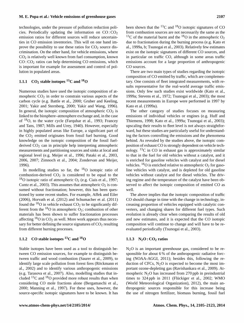
In the case of CO, the mole fractions at the tunnel exit area few tens of times larger than the ones at the entrance, thuswe can consider that essentially all CO observed at the exit isproduced by traffic. In this case we estimate the traffic signa-ture directly from the exit site data, without using the Keelingplot approach. Figure 4 shows theδ13C andδ18O in CO, withthe entrance and exit data shown in different colours. In theabsence of fractionation, the13C isotopic composition shouldbe the one of the fuel burnt, and the18O isotopic compositionshould derive from atmospheric O2.

δ13C in CO at the tunnel exit is consistently enriched com-pared to theδ13C value of the fuel of (−28.49± 0.06) ‰ asestimated from theδ13C in CO2 (assuming that13C in CO2represents the composition of the fuel, see previous section).The averageδ13C in CO for the exit site is (−25.6± 0.2) ‰.

For δ13C there is a subset of data that stands out of thegeneral trend, with CO more enriched in13C. These are the

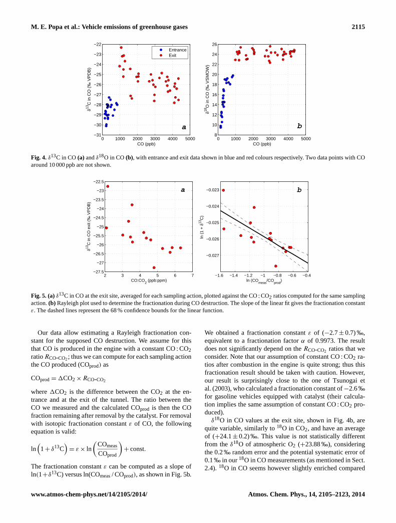
data with the lowest CO mole fractions from the tunnel exit.This suggests that the enrichment in13C in CO could takeplace not during the CO formation, but during its subsequentdestruction. Fig. 5 showsδ13C in CO at the exit site, aver-aged for each sampling action, plotted against the CO : CO2ratio of the same groups of flasks. Although quite noisy, atendency is evident of higherδ13C values for flasks that havea lower CO : CO2 ratio.

13C enrichment during CO destruction has been observedbefore by Tsunogai et al. (2003), who tested individual en-gines in various running and idling conditions. A similarphenomenon is documented for other gas species emittedby vehicles with catalyst, like N2O (Toyoda et al., 2008),CH4 (Chanton et al., 2000; Nakagawa et al., 2005) and H2(Vollmer et al., 2010). Although CO destruction takes placeboth in the engine and in the catalyst, it is most likely that the13C enrichment mainly happens in the catalyst, since it hasnot been observed in the case of vehicles without a catalyst(Tsunogai et al., 2003).



0 1000 2000 3000 4000 5000−31

−30

−29

−28

−27

−26

−25

−24

−23

−22

a

CO (ppb)

δ13C

in C

O (

‰ V

PD

B)

EntranceExit

0 1000 2000 3000 4000 50008

10

12

14

16

18

20

22

24

26

b

CO (ppb)

δ18O

in C

O (

‰ V

SM

OW

)

Fig. 4. δ13C in CO(a) andδ18O in CO(b), with entrance and exit data shown in blue and red colours respectively. Two data points with COaround 10 000 ppb are not shown.

2 3 4 5 6 7−27.5

−27

−26.5

−26

−25.5

−25

−24.5

−24

−23.5

−23

−22.5

CO:CO2 (ppb:ppm)

δ13C

in C

O e

xit (

‰ V

PD

B)

a

−1.6 −1.4 −1.2 −1 −0.8 −0.6 −0.4

−0.027

−0.026

−0.025

−0.024

−0.023

ln (COmeas

/COprod

)

ln (

1 +

δ13

C)

b

Fig. 5. (a)δ13C in CO at the exit site, averaged for each sampling action, plotted against the CO : CO2 ratios computed for the same samplingaction.(b) Rayleigh plot used to determine the fractionation during CO destruction. The slope of the linear fit gives the fractionation constantε. The dashed lines represent the 68 % confidence bounds for the linear function.

Our data allow estimating a Rayleigh fractionation con-stant for the supposed CO destruction. We assume for thisthat CO is produced in the engine with a constant CO : CO2ratioRCO-CO2; thus we can compute for each sampling actionthe CO produced (COprod) as

COprod = 1CO2 × RCO-CO2

where1CO2 is the difference between the CO2 at the en-trance and at the exit of the tunnel. The ratio between theCO we measured and the calculated COprod is then the COfraction remaining after removal by the catalyst. For removalwith isotopic fractionation constantε of CO, the followingequation is valid:

ln(1+ δ13C

)= ε × ln

(COmeas

COprod

)+ const.

The fractionation constantε can be computed as a slope ofln(1+δ13C) versus ln(COmeas/ COprod), as shown in Fig. 5b.

We obtained a fractionation constantε of (−2.7± 0.7) ‰,equivalent to a fractionation factorα of 0.9973. The resultdoes not significantly depend on theRCO-CO2 ratios that weconsider. Note that our assumption of constant CO : CO2 ra-tios after combustion in the engine is quite strong; thus thisfractionation result should be taken with caution. However,our result is surprisingly close to the one of Tsunogai etal. (2003), who calculated a fractionation constant of−2.6 ‰for gasoline vehicles equipped with catalyst (their calcula-tion implies the same assumption of constant CO : CO2 pro-duced).

δ18O in CO values at the exit site, shown in Fig. 4b, arequite variable, similarly to18O in CO2, and have an averageof (+24.1± 0.2) ‰. This value is not statistically differentfrom theδ18O of atmospheric O2 (+23.88 ‰), consideringthe 0.2 ‰ random error and the potential systematic error of0.1 ‰ in our18O in CO measurements (as mentioned in Sect.2.4). 18O in CO seems however slightly enriched compared



to the18O in CO2 (+23.57 ‰). Unlike theδ13C , the exit siteδ18O values do not depend on CO mole fractions; thus theyare not significantly affected during the CO destruction in thecatalytic converter.

Previous studies reported enrichment in18O in CO forgasoline vehicles with a functioning catalyst, and depletionin 18O for vehicles without a catalyst, for vehicles with cat-alyst during a cold start (when the catalyst is not yet func-tioning efficiently), and for diesel vehicles (e.g. Huff andThiemens, 1998; Kato et al., 1999a; Tsunogai et al., 2003).Our result integrates the emissions of many vehicles with po-tentially contrary effects, and the large variability in18O re-sults show that individual emitters could have very differentsignatures.

In summary, our fleet averaged results show net enrich-ment in13C relative to fuel and no significant difference in18O relative to atmospheric O2. For comparison, we show inFig. 6 our results together with results of several previousstudies that reported CO isotopic composition for the entirefleet, and separately for gasoline and diesel vehicles.

Part of the differences in13C among studies can probablybe explained by the different isotopic composition of the fuel.The results of our study and of Tsunogai et al. (2003) (Japanfleet, 2000) are similar and show the highestδ13C values forfleet averages; in addition, both studies find a13C enrichmentphenomenon during catalytic CO destruction. This could bethus a characteristic of modern vehicles and could probablybe related to the efficiency of catalytic destruction. Our18Oresults are very close to the ones of Tsunogai et al. (2003) andStevens et al. (1972) (world average, 1971), but differ signifi-cantly from the estimate of Kato et al. (1999a) (German fleet,1997).

As gasoline and diesel vehicles were reported to emit COwith very different isotopic signatures, the isotope valuesmeasured for the entire fleet could in principle be used to de-termine the relative emissions from gasoline and diesel vehi-cles. In the two studies shown in Fig. 6 that include separateestimates per fuel type, the fleet averages tend to be closer tothe gasoline signatures, which show a larger share of gaso-line emissions in the total CO. It would be useful to deter-mine the share of gasoline and diesel CO emissions for thepresent fleet, if data on isotopic signatures of recent vehiclesbecame available.

Modelling studies that include the isotopic composition ofCO (Bergamaschi et al., 2000; Manning et al., 1997) haveused until now, for the traffic-emitted CO, theδ13C andδ18Ovalues of fuel and atmospheric O2 respectively. Our studyadds to the already existing evidence that significant fraction-ation can occur during the formation and subsequent destruc-tion of CO, and that the traffic signatures can vary with timeand place. Better characterizing these signatures through ad-ditional measurements and updating the information used inmodels would help constraining the CO budget.

−32 −30 −28 −26 −24 −22 −20 −1810

12

14

16

18

20

22

24

26

28

δ13C in CO (‰ VPDB)

δ18O

in C

O (‰

VS

MO

W)

−30 −20 −1010

12

14

16

18

20

22

24

26This work Switzerland 2011Kato fleet Germany 1997Kato gasoline Germany 1997Kato diesel Germany 1997Tsunogai fleet Japan 2000Tsunogai gasoline Japan 2000Tsunogai diesel Japan 2000Tsunogai gasoline no−cat Japan 2000Stevens world average 1971

Fig. 6. δ18O versusδ13C in traffic CO from our work and previousstudies: Kato et al., 1999a (Kato); Tsunogai et al., 2003 (Tsunogai);Stevens et al., 1972 (Stevens). The year shown in legend is the yearwhen measurements were done. The dotted black lines indicate theδ18O in atmospheric oxygen (Barkan and Luz, 2005) and the aver-ageδ13C value of the fuel in our study, as estimated from theδ13Cvalue of CO2; the shades indicate their standard errors, and theirintersection shows the hypothetical CO isotopic composition in theabsence of fractionation. The CO isotopic composition of gasolinevehicles from Kato et al. (1999a) is based on vehicles without acatalyst and one vehicle with catalyst functioning with cold engine.

3.5 N2O : CO2 emission ratios

Figure 7 shows the1N2O:1CO2 ratios for the mole fractiondifferences of groups of exit-entrance flasks sampled at thesame time; the average ratio is (1.8± 0.2)× 10−2 ppb:ppm(equivalent for N2O : CO2 to mg:g). The results exhibit awide spread, with an upper limit of about 3× 10−2 ppb:ppm.The N2O : CO2 ratios seem to vary with the time of day andit is interesting to note that samples taken on different datesat about the same hour tend to give comparable results. How-ever no significant correlation was found with any of the traf-fic parameters available.

As the early morning data could have been influencedby N2O emissions outside the tunnel entrance in conditionsof slower air flow through the tunnel (see Sect. 3.1), wealso compute the N2O : CO2 ratios when removing the dataearlier than 08:30 LT. The N2O : CO2 average ratio is then(2.1± 0.1)× 10−2 ppb:ppm.

Table 2 summarizes results of traffic N2O : CO2 emissionratios from several previous studies. Our results are obvi-ously lower than all the previous ones, and it can be observedthat the N2O : CO2 ratios in Europe decreased monotonicallyover the past 20 yr. Since in general the emission of CO2per kilometre decreased, the N2O emission rate per kilome-tre travelled has decreased even more during this period thanthe N2O : CO2 ratio.

After the introduction of catalytic converters, it had beenobserved that vehicles fitted with a catalyst emitted moreN2O than older vehicles without a catalyst. N2O is formedat relatively low catalyst temperatures as an intermediate in



Table 2.Traffic emission N2O : CO2 ratios from various studies. The bold text shows the studies concerning European traffic.

Reference N2O : CO2 (g:g)× 105 Location Measurement year

Berges et al. (1993) 14± 9 Klara Tunnel, Sweden 1992Berges et al. (1993) 6± 3 Elbtunnel, Germany 1992Jimenez et al. (2000) 8.8± 2.8 Los Angeles, CA, USA 1996Jimenez et al. (2000) 12.8± 0.3 Manchester, NH, USA 1998Becker et al. (2000) 4.1± 1.2 Kiesberg Tunnel, Germany 1997Becker et al. (2000) 4.3± 1.2 Ford Research Laboratory (USA) 1996–1998Bradley et al. (2000) 18.7± 1.3 Denver, CO, USA 1997This study 1.8± 0.2 (2.1± 0.1)∗ Islisberg Tunnel, Switzerland 2011

∗ When excluding the early morning data.

00:00 06:00 12:00 18:00 00:000.005

0.01

0.015

0.02

0.025

0.03

time of day

ΔN2O

: ΔC

O2 (

ppb:

ppm

)

21−Jun−201122−Jun−201125−Jul−2011

Fig. 7.1N2O :1CO2 ratios for groups of exit-entrance flasks sam-pled in parallel, shown against time of day. Different colours indi-cate different sampling dates.

nitrogen oxides reduction. The concern appeared that thequantity of N2O emitted by traffic would increase with theincreasing proportion of catalyst vehicles (e.g. Berges et al.,1993; Dasch, 1992). Our study clearly does not support thisconcern; on the contrary, we find for the present fleet sig-nificantly lower N2O : CO2 emission ratios than reported inthe past. This is in line with the decreasing trend already ob-served from the study of Becker et al. (2000), when com-pared to the older ones. We assume that with improving cat-alytic technology, less N2O is produced and a larger propor-tion of N2O is completely reduced.

The following issue may affect our N2O : CO2 emissionratio estimate. N2O can be formed inside containers fromNOx, in the presence of water and SO2, with a time constantfor N2O formation on the order of hours; for dried samplesthe effect is smaller but is still present (Muzio et al., 1989).Since NOx, SO2 and water are present in vehicle emissionsand consequently increased in the tunnel atmosphere, it ispossible that part of the N2O excess we observed is not di-

rectly emitted by vehicles but formed later either in the tunnelor inside the glass flasks during the few months’ storage. Inthis case our estimate is a sum of direct and indirect trafficemissions in tunnel conditions. If N2O resulted from NOxmakes a significant proportion, then in open air conditionsthe total traffic-resulted N2O may be even lower than our es-timate.

3.6 CH4 : CO2 emission ratios

As already mentioned, the variability in the CH4 mole frac-tions of the air entering the tunnel is large compared to thetraffic signal (see Fig. 1). Thus, for the1CH4 : 1CO2 ratios,we only used the afternoon data, when the CH4 variabilityat the entrance was smallest, because we considered that theother data would give unreliable CH4 : CO2 emission ratioresults. This leaves us with only seven data points for theCH4 : CO2 emission ratios (not shown in figures); the aver-age1CH4 : 1CO2 ratio is (4.6± 0.2)× 10−2 ppb:ppm.

It is general knowledge that vehicles emit small quan-tities of methane, and (indirect) measurements of methaneare included in certification vehicle testing, but we are notaware of comprehensive studies focusing on the recent Eu-ropean vehicle fleet. We can compare our results to theones of Nam et al. (2004), who performed measurementson US vehicles of model years 1995 to 1999. For hot run-ning vehicles, they obtained an average1CH4 : 1CO2 ratioof 3.8× 10−2 ppb:ppm, which is close to our result. Theiroverall result that includes cold start emissions is much larger(14× 10−2 ppb:ppm); this supports that, for estimating theoverall traffic CH4 : CO2 emission ratios, other traffic condi-tions must be taken into account.

Nakagawa et al. (2005) estimated the contribution of traf-fic emissions to the total CH4 fluxes to be up to 30 % in aJapanese large urban area (based on isotope measurements).In our case it is obvious that the mole fraction increase dueto traffic emissions (represented by the difference betweenthe tunnel exit and entrance) is small compared to the over-all variability; thus the traffic emissions account for a muchsmaller proportion of the total CH4 fluxes.



3.7 O2 : CO2 ratios

As obvious in Fig. 1, variations in O2 / N2 ratios areanti-correlated to the CO2 variations. Figure 8 shows the1O2 : 1CO2 ratios computed from groups of exit-entranceflasks sampled in parallel. All1O2 : 1CO2 ratios lie withinthe narrow interval−1.48 to −1.46, with an average of−1.47± 0.01 ppm:ppm.

Overall our1O2 : 1CO2 results are similar to the ratiosof approximately−1.5 calculated theoretically based on fuelcomposition by Steinbach et al. (2011) for this region. Wenote that the oxidative ratios from Steinbach et al. (2011) in-clude other fossil fuel burning processes, not only road traf-fic.

Interestingly, our1O2 : 1CO2 ratios are also very close tothe average reduction level (or oxidative ratio) of the fuelburnt of 1.5± 0.06 obtained by Keeling (1988), based onO2 and CO2 simultaneous measurements in an urban atmo-sphere dominated by traffic. For determining the reductionlevel, Keeling (1988) corrected the measured1O2 : 1CO2ratios, assuming that a proportion of (8.5± 8.5) % of the car-bon in fuel is emitted as CO. With the actual technology inEurope, a much smaller proportion of the fuel is burnt to CO(see Sect. 3.2); thus we can consider that the1O2 : 1CO2 ra-tios we obtained directly represent the reduction level of thefuel burnt, without a correction being necessary.

4 Summary and final remarks

The main results of our paper can be summarized as follows.

a. The CO : CO2 emission ratios, with an averageof (4.15± 0.34) ppb:ppm, are lower than the ratiospresently available from databases and used in models,and than older experimental estimates. This is proba-bly due to the evolution of the vehicle fleet associatedwith the evolution of vehicle emission standards. TheCO : CO2 emission ratio is likely to continue decreas-ing in the future, as older vehicles are replaced by newones, thus it will have to be continuously updated ifused for estimating the fossil fuel CO2.

b. According to our measurements, theδ18O in traffic-emitted CO2 has an average value of+23.6 ‰, andthus is depleted by 0.3 ‰ relative to the atmosphericO2. The variability of ourδ18O-CO2 data suggests thepossibility that individual vehicles do emit CO2 withdifferent δ18O signatures, which is in line with mea-surements of individual vehicles in other studies. How-ever, our results do not show a large systematic devia-tion in δ18O-CO2 at fleet level.

c. δ13C in CO is enriched by 3 ‰ compared to the iso-topic composition of the fuel, and its variability seemsto be dominated by a destruction phenomenon in thecatalyst, with highestδ13C values associated to low

00:00 06:00 12:00 18:00 00:00−1.49

−1.485

−1.48

−1.475

−1.47

−1.465

−1.46

−1.455

−1.45

−1.445

time of day

ΔO2:Δ

CO

2 rat

io (

ppm

:ppm

)

21−Jun−201122−Jun−201125−Jul−2011

Fig. 8. 1O2 : 1CO2 ratios for groups of exit-entrance flasks sam-pled in parallel, shown against time of day. Different colours indi-cate different sampling dates. The negative ratios are due to the factthat O2 is consumed while CO2 is produced.

CO : CO2 emission ratios. Forδ13C we compute a frac-tionation constantε of (−2.7± 0.7) ‰ for the catalyticCO oxidation.δ18O in CO is similar within the un-certainty to the isotopic composition of atmosphericO2, and, unlikeδ13C, is not correlated to the CO : CO2emission ratios.

A potential application of integrated fleet measure-ments of CO isotopic composition is to estimate therelative contribution of emissions from gasoline anddiesel vehicles; for this, more knowledge on the iso-topic signature of CO emitted from recent vehicles isnecessary.

d. The N2O : CO2 emission ratios of (1.8± 0.2) × 0−2

ppb:ppm ((2.1± 0.1)× 10−2 ppb:ppm when excludingthe early morning data) are lower than older estimates,suggesting a decrease in N2O emissions with improv-ing technology. The concern that N2O emissions willincrease with the proportion of vehicles fitted with cat-alyst converters is not supported by our results. It ispossible that the technological improvements will leadto an even further decrease in traffic N2O emissions.

e. We find an average CH4 : CO2 emission ratio of(4.6± 0.2)× 10−2 ppb:ppm. Our results confirm thatthe traffic CH4 source is small compared to the otheremissions.

f. The 1O2 : 1CO2 ratios from traffic emissions of(−1.47± 0.01) ppm:ppm are very close to previoustheoretical and experimental estimates.

The main limitations of our study are as follows. (1)The fleet composition in the Islisberg Tunnel during our



campaign may be different from the fleet composition inother locations in Europe and not fully representative for theoverall European fleet. Thus our results may not be repre-sentative for different places and times, and an upscaling ofour results to the entire western Europe must be done withcaution. (2) The tunnel has a highway driving regime and thetraffic was fluent during our measurement campaign. In dif-ferent traffic conditions, like in urban areas or during trafficjams, emissions and the ratios between the emitted speciesare likely to be different. Emission rates reported for suchcases are usually higher.

We recommend

– a periodical update of CO : CO2 emission ratios if theyare to be used for quantifying fossil fuel contributions;

– further studies on the possibility of using CO isotopesto distinguish between emission sources, and the pos-sibilities of combining this with other tracers; for thispurpose more information is needed on the isotopicsignatures of CO sources and sinks;

– more studies characterizing the isotopic signature oftraffic (and other fossil fuel) derived CO2 to addressthe discrepancy between modelling studies that as-sume that burning processes occur without significantfractionation, and measurements that find fractionationinduced alterations of CO2 isotopic signatures;

– complementary studies for estimating traffic emissionsin different conditions that are necessary to completethe picture: locations with different fleet composition,traffic type (e.g. city or traffic jams), and atmosphericconditions (e.g. different temperatures during winter);

– increasing the number of atmospheric oxygen mea-surements and testing new possibilities to use oxy-gen data for distinguishing between sources and sinks,making use of the well-defined O2 : CO2 ratios for cer-tain combustion processes.

Supplementary material related to this article isavailable online athttp://www.atmos-chem-phys.net/14/2105/2014/acp-14-2105-2014-supplement.zip.

Acknowledgements.The authors would like to thank the follow-ing colleagues for support during sampling and measurements:Michel Bolder and Carina van der Veen (IMAU), Matz Hill (Empa),Bert Steinberg and Juergen Richter (MPI-BGC).

We thank Urs Schaufelberger and Markus Meier(AWEL/WWEA) for sharing their sampling lines and forgeneral support.

The travel of M. E. Popa to Switzerland for the sampling cam-paign has been financially supported by the European Science Foun-dation (ESF), in the framework of the Research Networking Pro-gramme TTORCH. The measurements of flask samples at MPI-BGC were funded by the FP6 project IMECC, Transnational AccessActivity TA1. This work has received additional support from theNWO projects 053.61.026 and 865.07.001 and from the EU projectINTRAMIF.

We thank Hans Coops for useful comments on the manuscript.

Edited by: R. Harley

References

Affek, H. P. and Eiler, J. M.: Abundance of mass 47 CO2 in urbanair, car exhaust, and human breath, Geochim Cosmochim Ac, 70,1–12, doi:10.1016/j.gca.2005.08.021, 2006.

Andreae, M. O. and Merlet, P.: Emission of trace gases and aerosolsfrom biomass burning, Global Biogeochem. Cy., 15, 955–966,doi:10.1029/2000GB001382, 2001.

Angelbratt, J., Mellqvist, J., Simpson, D., Jonson, J. E., Blumen-stock, T., Borsdorff, T., Duchatelet, P., Forster, F., Hase, F.,Mahieu, E., De Mazière, M., Notholt, J., Petersen, A. K., Raffal-ski, U., Servais, C., Sussmann, R., Warneke, T., and Vigouroux,C.: Carbon monoxide (CO) and ethane (C2H6) trends fromground-based solar FTIR measurements at six European stations,comparison and sensitivity analysis with the EMEP model, At-mos. Chem. Phys., 11, 9253–9269, doi:10.5194/acp-11-9253-2011, 2011.

Barkan, E. and Luz, B.: High precision measurements of17O/16Oand 18O/16O ratios in H2O, Rapid Commun. Mass. Sp., 19,3737–3742, doi:10.1002/rcm.2250, 2005.

Battle, M., Bender, M. L., Tans, P. P., White, J. W. C., Ellis, J. T.,Conway, T., and Francey, R. J.: Global carbon sinks and theirvariability inferred from atmospheric O2 andδ13C, Science, 287,2467–2470, doi:10.1126/science.287.5462.2467, 2000.

Battle, M., Fletcher, S. M., Bender, M. L., Keeling, R. F.,Manning, A. C., Gruber, N., Tans, P. P., Hendricks, M. B.,Ho, D. T., and Simonds, C.: Atmospheric potential oxygen:New observations and their implications for some atmosphericand oceanic models, Global Biogeochem. Cy., 20, GB1010,doi:10.1029/2005GB002534, 2006.

Becker, K. H., Lörzer, J. C., Kurtenbach, R., Wiesen, P., Jensen, T.E., and Wallington, T. J.: Contribution of vehicle exhaust to theglobal N2O budget, Chemosphere – Global Change Science, 2,387–395, doi:10.1016/S1465-9972(00)00017-9, 2000.

Bender, M. L., Ho, D. T., Hendricks, M. B., Mika, R., Battle, M. O.,Tans, P. P., Conway, T. J., Sturtevant, B., and Cassar, N.: Atmo-spheric O2 / N2 changes, 1993–2002: Implications for the par-titioning of fossil fuel CO2 sequestration, Global Biogeochem.Cy., 19, GB4017, doi:10.1029/2004GB002410, 2005.


http://www.atmos-chem-phys.net/14/2105/2014/acp-14-2105-2014-supplement.zip

http://www.atmos-chem-phys.net/14/2105/2014/acp-14-2105-2014-supplement.zip

http://dx.doi.org/10.1016/j.gca.2005.08.021

http://dx.doi.org/10.1029/2000GB001382

http://dx.doi.org/10.5194/acp-11-9253-2011


http://dx.doi.org/10.1002/rcm.2250

http://dx.doi.org/10.1126/science.287.5462.2467

http://dx.doi.org/10.1029/2005GB002534

http://dx.doi.org/10.1016/S1465-9972(00)00017-9

http://dx.doi.org/10.1029/2004GB002410


Bergamaschi, P., Hein, R., Brenninkmeijer, C. A. M., and Crutzen,P. J.: Inverse modeling of the global CO cycle, 2. Inversion of13C /12C and 18O/16O isotope ratios, J. Geophys. Res., 105,1929–1946, doi:10.1029/1999JD900819, 2000.

Berges, M. G. M., Hofmann, R. M., Scharffe, D., and Crutzen, P.J.: Nitrous oxide emissions from motor vehicles in tunnels andtheir global extrapolation, J. Geophys. Res.-Atmos., 98, 18527–18531, doi:10.1029/93jd01637, 1993.

Bishop, G. A. and Stedman, D. H.: A decade of on-road emis-sions measurements, Environ. Sci. Technol., 42, 1651–1656,doi:10.1021/es702413b, 2008.

Bradley, K. S., Brooks, K. B., Hubbard, L. K., Popp, P. J., and Sted-man, D. H.: Motor vehicle fleet emissions by OP-FTIR, Environ.Sci. Technol., 34, 897–899, doi:10.1021/es9909226, 2000.

Brand, W. A.: O2 / N2 storage aspects and open split mass spectro-metric determination, in: Proceedings of the 12th IAEA/WMOmeeting of CO2 experts, Toronto, Sept. 2003, edited by: Worthy,D., and Huang, L., WMO-GAW Report 161, 146–151, 2005.

Brand, W. A., Huang, L., Mukai, H., Chivulescu, A., Richter, J.M., and Rothe, M.: How well do we know VPDB? Variabilityof δ13C andδ18O in CO2 generated from NBS19-calcite., RapidCommun. Mass. Sp., 23, 915–926, doi:10.1002/rcm.3940, 2009.

Brenninkmeijer, C. A. M.: Measurement of the abundance of14COin the atmosphere and the13C /12C and18O/16O ratio of atmo-spheric CO with applications in New Zealand and Antarctica,J. Geophys. Res., 98, 10595–10614, doi:10.1029/93JD00587,1993.

Cant, N. W., Angove, D. E., and Chambers, D. C.: Nitrous ox-ide formation during the reaction of simulated exhaust streamsover rhodium, platinum and palladium catalysts, Appl. CatalB-Environ., 17, 63–73, doi:10.1016/S0926-3373(97)00105-7,1998.

Chanton, J. P., Rutkowski, C. M., Schwartz, C. C., Ward, D. E., andBoring, L.: Factors influencing the stable carbon isotopic signa-ture of methane from combustion and biomass burning, J. Geo-phys. Res.-Atmos., 105, 1867–1877, doi:10.1029/1999jd900909,2000.

Ciais, P., Denning, A. S., Tans, P. P., and Berry, J. A.: A three-dimensional synthesis study of in atmospheric CO2, J. Geophys.Res., 102, 5857–5872, doi:10.1029/96JD02360, 1997.

Cuntz, M., Ciais, P., Hoffmann, G., and Knorr, W.: A compre-hensive global three-dimensional model ofδ18O in atmosphericCO2: 1. Validation of surface processes, J. Geophys. Res.-Atmos., 108, 4527, doi:10.1029/2002jd003153, 2003.

Dasch, J. M.: Nitrous Oxide Emissions from Vehicles, J. Air WasteManage., 42, 63–67, doi:10.1080/10473289.1992.10466971,1992.

EEA: www.eea.europa.eu/data-and-maps/figures/sector-contributions-of-ozone-precursor-2, 2013.

Etheridge, D. M., Steele, L. P., Francey, R. J., and Lan-genfelds, R. L.: Atmospheric methane between 1000 A.D.and present: Evidence of anthropogenic emissions and cli-matic variability, J. Geophys. Res.-Atmos., 103, 15979–15993,doi:10.1029/98jd00923, 1998.

Farquhar, G. D., Lloyd, J., Taylor, J. A., Flanagan, L. B., Syvertsen,J. P., Hubick, K. T., Wong, S. C., and Ehleringer, J. R.: Vegeta-tion effects on the isotope composition of oxygen in atmosphericCO2, Nature, 363, 439–443, doi:10.1038/363439a0, 1993.

Flückiger, J., Monnin, E., Stauffer, B., Schwander, J., Stocker,T. F., Chappellaz, J., Raynaud, D., and Barnola, J. M.: High-resolution Holocene N2O ice core record and its relation-ship with CH4 and CO2, Global Biogeochem. Cy., 16, 1010,doi:10.1029/2001GB001417, 2002.

Forster, P., Ramaswamy, V., Artaxo, P., Berntsen, T., Betts, R., Fa-hey, D. W., Haywood, J., Lean, J., Lowe, D. C., Myhre, G.,Nganga, J., Prinn, R., Raga, G., Schultz, M., and Van Dorland,R.: Changes in Atmospheric Constituents and in Radiative Forc-ing, in: Climate Change 2007: The Physical Science Basis. Con-tribution of Working Group I to the Fourth Assessment Reportof the Intergovernmental Panel on Climate Change, edited by:Solomon, S., Qin, D., Manning, M., Chen, Z., Marquis, M., Av-eryt, K. B., Tignor, M., and Miller, H. L., Cambridge UniversityPress, Cambridge, United Kingdom, 2007.

Francey, R. J. and Tans, P. P.: Latitudinal variation in oxygen-18 ofatmospheric CO2, Nature, 327, 495–497, doi:10.1038/327495a0,1987.

Friedman, I. and O’Neil, J. R.: Compilation of stable isotope frac-tionation factors of geochemical interest, USGPO, 1977.

Gamnitzer, U., Karstens, U., Kromer, B., Neubert, R. E. M., Mei-jer, H. A. J., Schroeder, H., and Levin, I.: Carbon monoxide: Aquantitative tracer for fossil fuel CO2?, J. Geophys. Res.-Atmos.,111, D22302, doi:10.1029/2005jd006966, 2006.

Ghosh, P., Patecki, M., Rothe, M., and Brand, W. A.: Calcite-CO2mixed into CO2-free air: a new CO2-in-air stable isotope refer-ence material for the VPDB scale, Rapid Commun Mass. Sp., 19,1097–1119, 2005.

Granier, C., Bessagnet, B., Bond, T., D’Angiola, A., Denier van derGon, H., Frost, G., Heil, A., Kaiser, J., Kinne, S., Klimont, Z.,Kloster, S., Lamarque, J.-F., Liousse, C., Masui, T., Meleux, F.,Mieville, A., Ohara, T., Raut, J.-C., Riahi, K., Schultz, M., Smith,S., Thompson, A., Aardenne, J., Werf, G., and Vuuren, D.: Evolu-tion of anthropogenic and biomass burning emissions of air pol-lutants at global and regional scales during the 1980–2010 pe-riod, Climatic Change, 109, 163–190, doi:10.1007/s10584-011-0154-1, 2011.

Graven, H. D., Stephens, B. B., Guilderson, T. P., Campos, T.L., Schimel, D. S., Campbell, J. E., and Keeling, R. F.: Verti-cal profiles of biospheric and fossil fuel-derived CO2 and fos-sil fuel CO2 : CO ratios from airborne measurements of114C,CO2 and CO above Colorado, USA, Tellus B, 61, 536–546,doi:10.1111/j.1600-0889.2009.00421.x, 2009.

Gruber, N. and Keeling, C. D.: An improved estimate of the iso-topic air-sea disequilibrium of CO2: Implications for the oceanicuptake of anthropogenic CO2, Geophys. Res. Lett., 28, 555–558,doi:10.1029/2000GL011853, 2001.

Horvath, B., Hofmann, M. E. G., and Pack, A.: On the triple oxy-gen isotope composition of carbon dioxide from some com-bustion processes, Geochim. Cosmochim. Ac., 95, 160–168,doi:10.1016/j.gca.2012.07.021, 2012.

Huff, A. K. and Thiemens, M. H.:170/160 and180/160 isotope mea-surements of atmospheric carbon monoxide and its sources, Geo-phys. Res. Lett., 25, 3509–3512, doi:10.1029/98GL02603, 1998.

IPCC: Revised 1996 IPCC Guidelines for National Greenhouse GasInventories, Intergovernmental Panel on Climate Change,www.ipcc-nggip.iges.or.jp/public/gl/invs1.html, 1997.

Jimenez, J. L., McManus, J. B., Shorter, J. H., Nelson, D. D.,Zahniser, M. S., Koplow, M., McRae, G. J., and Kolb, C. E.:


http://dx.doi.org/10.1029/1999JD900819

http://dx.doi.org/10.1029/93jd01637

http://dx.doi.org/10.1021/es702413b

http://dx.doi.org/10.1021/es9909226


http://dx.doi.org/10.1029/93JD00587

http://dx.doi.org/10.1016/S0926-3373(97)00105-7

http://dx.doi.org/10.1029/1999jd900909

http://dx.doi.org/10.1029/96JD02360

http://dx.doi.org/10.1029/2002jd003153

http://dx.doi.org/10.1080/10473289.1992.10466971

www.eea.europa.eu/data-and-maps/figures/sector-contributions-of-ozone-precursor-2

www.eea.europa.eu/data-and-maps/figures/sector-contributions-of-ozone-precursor-2


http://dx.doi.org/10.1038/363439a0

http://dx.doi.org/10.1029/2001GB001417

http://dx.doi.org/10.1038/327495a0

http://dx.doi.org/10.1029/2005jd006966

http://dx.doi.org/10.1007/s10584-011-0154-1

http://dx.doi.org/10.1007/s10584-011-0154-1

http://dx.doi.org/10.1111/j.1600-0889.2009.00421.x

http://dx.doi.org/10.1029/2000GL011853

http://dx.doi.org/10.1016/j.gca.2012.07.021

http://dx.doi.org/10.1029/98GL02603

www.ipcc-nggip.iges.or.jp/public/gl/invs1.html

www.ipcc-nggip.iges.or.jp/public/gl/invs1.html


Cross road and mobile tunable infrared laser measurementsof nitrous oxide emissions from motor vehicles, Chemosphere– Global Change Science, 2, 397–412, doi:10.1016/S1465-9972(00)00019-2, 2000.

Jordan, A. and Brand, W. A.: Technical Report: MPI-BGC, Ger-many, in: Proceedings of the 11th IAEA/WMO meeting of CO2experts, Tokyo, September 2001, edited by: Toru, S., WMO-GAW Report 148, 149–153, 2003.

Jordan, A. and Steinberg, B.: Calibration of atmospheric hy-drogen measurements, Atmos. Meas. Tech., 4, 509–521,doi:10.5194/amt-4-509-2011, 2011.

Kato, S., Akimoto, H., Braunlich, M., Rockmann, T., and Bren-ninkmeijer, C. A. M.: Measurements of stable carbon and oxygenisotopic compositions of CO in automobile exhausts and ambientair from semi-urban Mainz, Germany, Geochem. J., 33, 73–77,doi:10.2343/geochemj.33.73, 1999a.

Kato, S., Akimoto, H., Rockmann, T., Braunlich, M., and Bren-ninkmeijer, C. A. M.: Stable isotopic compositions of carbonmonoxide from biomass burning experiments, Atmos. Environ.,33, 4357–4362, doi:10.1016/S1352-2310(99)00243-5, 1999b.

Keeling, R. F.: Measuring Correlations between AtmosphericOxygen and Carbon Dioxide Mole Fractions: a Prelimi-nary Study in Urban Air, J. Atmos. Chem., 7, 153–176,doi:10.1007/Bf00048044, 1988.

Keeling, R. F. and Shertz, S. R.: Seasonal and interannual variationsin atmospheric oxygen and implications for the global carboncycle, Nature, 358, 723–727, doi:10.1038/358723a0, 1992.

Keeling, R. F., Najjar, R. P., Bender, M. L., and Tans, P. P.:What atmospheric oxygen measurements can tell us aboutthe global carbon cycle, Global Biogeochem. Cy., 7, 37–67,doi:10.1029/92gb02733, 1993.

Keeling, R. F., Piper, S. C., and Heimann, M.: Global and hemi-spheric CO2 sinks deduced from changes in atmospheric O2 con-centration, Nature, 381, 218–221, doi:10.1038/381218a0, 1996.

Keeling, R. F., Blaine, T., Paplawsky, B., Katz, L., Atwood, C.,and Brockwell, T.: Measurement of changes in atmosphericA / N2 ratio using a rapid-switching, single-capillary mass spec-trometer system, Tellus B, 56, 322–338, doi:10.1111/j.1600-0889.2004.00117.x, 2004.

Levin, I. and Karstens, U.: Inferring high-resolution fossil fuelCO2 records at continental sites from combined14CO2 andCO observations, Tellus B, 59, 245–250, doi:10.1111/j.1600-0889.2006.00244.x, 2007.

Lipman, T. E. and Delucchi, M. A.: Emissions of nitrous oxide andmethane from conventional and alternative fuel motor vehicles,Climatic Change, 53, 477–516, doi:10.1023/A:1015235211266,2002.

Manning, M. R., Brenninkmeijer, C. A. M., and Allan, W.: Atmo-spheric carbon monoxide budget of the southern hemisphere: Im-plications of13C /12C measurements, J. Geophys. Res.-Atmos.,102, 10673–10682, doi:10.1029/96jd02743, 1997.

Manning, A. C. and Keeling, R. F.: Global oceanic and land bi-otic carbon sinks from the Scripps atmospheric oxygen flasksampling network, Tellus B, 58, 95–116, doi:10.1111/j.1600-0889.2006.00175.x, 2006.

Meijer, H. A. J., Smid, H. M., Perez, E., and Keizer, M. G.: Iso-topic characterisation of anthropogenic CO2 emissions using iso-topic and radiocarbon analysis, Phys. Chem. Earth, 21, 483–487,doi:10.1016/S0079-1946(97)81146-9, 1996.

Mills, G. A. and Urey, H. C.: The kinetics of isotopic exchange be-tween carbon dioxide, bicarbonate ion, carbonate ion and water,J. Am. Chem. Soc., 62, 1019–1026, doi:10.1021/Ja01862a010,1940.

Muzio, L. J., Teague, M. E., Kramlich, J. C., Cole, J. A., Mc-Carthy, J. M., and Lyon, R. K.: Errors in Grab Sample Measure-ments of N2O from Combustion Sources, JAPCA, 39, 287–293,doi:10.1080/08940630.1989.10466528, 1989.

Nakagawa, F., Tsunogai, U., Komatsu, D. D., Yamada, K., Yoshida,N., Moriizumi, J., Nagamine, K., Iida, T., and Ikebe, Y.: Auto-mobile exhaust as a source of13C- and D-enriched atmosphericmethane in urban areas, Organic Geochemistry, 36, 727–738,doi:10.1016/j.orggeochem.2005.01.003, 2005.

Nam, E. K., Jensen, T. E., and Wallington, T. J.: Methane Emis-sions from Vehicles, Environ. Sci. Technol., 38, 2005–2010,doi:10.1021/es034837g, 2004.

NOAA-AGGI 2011: http://www.esrl.noaa.gov/gmd/aggi, last ac-cess: March 2011.

Pataki, D. E., Bowling, D. R., and Ehleringer, J. R.: Seasonal cycleof carbon dioxide and its isotopic composition in an urban atmo-sphere: Anthropogenic and biogenic effects, J. Geophys. Res.-Atmos., 108, 4735, doi:10.1029/2003jd003865, 2003.

Pataki, D. E., Bowling, D. R., Ehleringer, J. R., and Zob-itz, J. M.: High resolution atmospheric monitoring of ur-ban carbon dioxide sources, Geophys. Res. Lett., 33, L03813,doi:10.1029/2005gl024822, 2006.

Pataki, D. E, Xu, T., Luo, Y. Q, and Ehleringer, J. R: Inferring bio-genic and anthropogenic carbon dioxide sources across an urbanto rural gradient, Oecologia, 152, 307–322, doi:10.1007/s00442-006-0656-0, 2007.

Pathirana, S. L and Röckmann, T.: An analytical system for study-ing the stable isotopes of carbon monoxide using ContinuousFlow – Isotope Ratio Mass Spectroscopy (CF-IRMS), in prepa-ration, 2014.

Pfister, G., Pétron, G., Emmons, L. K., Gille, J. C., Edwards,D. P., Lamarque, J. F., Attie, J. L., Granier, C., and Novelli,P. C.: Evaluation of CO simulations and the analysis of theCO budget for Europe, J. Geophys. Res.-Atmos., 109, D19304,doi:10.1029/2004jd004691, 2004.

Ravishankara, A., Daniel, J. S., and Portmann, R. W.: Ni-trous oxide (N2O): The dominant ozone-depleting sub-stance emitted in the 21st century, Science, 326, 123–125,doi:10.1126/science.1176985, 2009.

Rhys-Tyler, G. A., Legassick, W., and Bell, M. C.: The significanceof vehicle emissions standards for levels of exhaust pollutionfrom light vehicles in an urban area, Atmos Environ, 45, 3286–3293, doi:10.1016/j.atmosenv.2011.03.035, 2011.

Rivier, L., Ciais, P., Hauglustaine, D. A., Bakwin, P., Bousquet, P.,Peylin, P., and Klonecki, A.: Evaluation of SF6, C2Cl4, and COto approximate fossil fuel CO2 in the Northern Hemisphere us-ing a chemistry transport model, J. Geophys. Res., 111, D16311,doi:10.1029/2005JD006725, 2006.

Röckmann, T., Jöckel, P., Gros, V., Bräunlich, M., Possnert, G., andBrenninkmeijer, C. A. M.: Using14C, 13C, 18O and17O iso-topic variations to provide insights into the high northern lat-itude surface CO inventory, Atmos. Chem. Phys., 2, 147–159,doi:10.5194/acp-2-147-2002, 2002.

Röckmann, T., Gómez Álvarez, C. X., Walter, S., Veen, C. v.,Wollny, A. G., Gunthe, S. S., Helas, G., Pöschl, U., Keppler,


http://dx.doi.org/10.1016/S1465-9972(00)00019-2

http://dx.doi.org/10.1016/S1465-9972(00)00019-2

http://dx.doi.org/10.5194/amt-4-509-2011

http://dx.doi.org/10.2343/geochemj.33.73

http://dx.doi.org/10.1016/S1352-2310(99)00243-5

http://dx.doi.org/10.1007/Bf00048044

http://dx.doi.org/10.1038/358723a0

http://dx.doi.org/10.1029/92gb02733

http://dx.doi.org/10.1038/381218a0

http://dx.doi.org/10.1111/j.1600-0889.2004.00117.x

http://dx.doi.org/10.1111/j.1600-0889.2004.00117.x

http://dx.doi.org/10.1111/j.1600-0889.2006.00244.x

http://dx.doi.org/10.1111/j.1600-0889.2006.00244.x

http://dx.doi.org/10.1023/A:1015235211266


http://dx.doi.org/10.1111/j.1600-0889.2006.00175.x

http://dx.doi.org/10.1111/j.1600-0889.2006.00175.x

http://dx.doi.org/10.1016/S0079-1946(97)81146-9

http://dx.doi.org/10.1021/Ja01862a010

http://dx.doi.org/10.1080/08940630.1989.10466528

http://dx.doi.org/10.1016/j.orggeochem.2005.01.003

http://dx.doi.org/10.1021/es034837g

http://www.esrl.noaa.gov/gmd/aggi

http://dx.doi.org/10.1029/2003jd003865

http://dx.doi.org/10.1029/2005gl024822

http://dx.doi.org/10.1007/s00442-006-0656-0

http://dx.doi.org/10.1007/s00442-006-0656-0

http://dx.doi.org/10.1029/2004jd004691

http://dx.doi.org/10.1126/science.1176985

http://dx.doi.org/10.1016/j.atmosenv.2011.03.035

http://dx.doi.org/10.1029/2005JD006725



F., Greule, M., and Brand, W. A.: The isotopic composition ofH2 from wood burning – dependency on combustion efficiency,moisture content andδD of local precipitation, J. Geophys. Res.,115, D17308, doi:17310.11029/12009JD013188, 2010.

Ropkins, K., Beebe, J., Li, H., Daham, B., Tate, J., Bell, M., andAndrews, G.: Real-World Vehicle Exhaust Emissions Monitor-ing: Review and Critical Discussion, Crit. Rev. Env. Sci. Tec.,39, 79–152, doi:10.1080/10643380701413377, 2009.

Saurer, M., Prévôt, A. S. H., Dommen, J., Sandradewi, J., Bal-tensperger, U., and Siegwolf, R. T. W.: The influence of traf-fic and wood combustion on the stable isotopic composi-tion of carbon monoxide, Atmos. Chem. Phys., 9, 3147–3161,doi:10.5194/acp-9-3147-2009, 2009.

Schumacher, M., Werner, R. A., Meijer, H. A. J., Jansen, H. G.,Brand, W. A., Geilmann, H., and Neubert, R. E. M.: Oxygenisotopic signature of CO2 from combustion processes, Atmos.Chem. Phys., 11, 1473–1490, doi:10.5194/acp-11-1473-2011,2011.

Steinbach, J., Gerbig, C., Rödenbeck, C., Karstens, U., Minejima,C., and Mukai, H.: The CO2 release and Oxygen uptake fromFossil Fuel Emission Estimate (COFFEE) dataset: effects fromvarying oxidative ratios, Atmos. Chem. Phys., 11, 6855–6870,doi:10.5194/acp-11-6855-2011, 2011.

Stephens, B. B., Keeling, R. F., and Paplawsky, W. J.: Ship-board measurements of atmospheric oxygen using a vacuum-ultraviolet absorption technique, Tellus B, 55, 857–878,doi:10.1046/j.1435-6935.2003.00075.x, 2003.

Stevens, C. M., Krout, L., Walling, D., Venters, A., Engelke-meir, A., and Ross, L. E.: The isotopic composition of atmo-spheric carbon monoxide, Earth Planet. Sci. Lett., 16, 147–165,doi:10.1016/0012-821X(72)90183-5, 1972.

Suntharalingam, P., Jacob, D. J., Palmer, P. I., Logan, J. A., Yan-tosca, R. M., Xiao, Y. P., Evans, M. J., Streets, D. G., Vay, S. L.,and Sachse, G. W.: Improved quantification of Chinese carbonfluxes using CO2/CO correlations in Asian outflow, J. Geophys.Res.-Atmos., 109, D18S18, doi:10.1029/2003jd004362, 2004.

Tarasova, O. A., Brenninkmeijer, C. A. M., Assonov, S. S., Elan-sky, N. F., Röckmann, T., and Sofiev, M. A.: Atmospheric COalong the Trans-Siberian Railroad and River Ob: source identi-fication using isotope analysis, J. Atmos. Chem., 57, 135–152,doi:10.1007/s10874-007-9066-x, 2007.

Toyoda, S., Yamamoto, S., Arai, S., Nara, H., Yoshida, N., Kashi-wakura, K., and Akiyama, K.: Isotopomeric characterization ofN2O produced, consumed, and emitted by automobiles, RapidCommun. Mass. Sp., 22, 603–612, doi:10.1002/rcm.3400, 2008.

Tsunogai, U., Hachisu, Y., Komatsu, D. D., Nakagawa, F.,Gamo, T., and Akiyama, K.: An updated estimation ofthe stable carbon and oxygen isotopic compositions of au-tomobile CO emissions, Atmos. Environ., 37, 4901–4910,doi:10.1016/j.atmosenv.2003.08.008, 2003.

Turnbull, J. C., Miller, J. B., Lehman, S. J., Tans, P. P., Sparks, R. J.,and Southon, J.: Comparison of14CO2, CO, and SF6 as tracersfor recently added fossil fuel CO2 in the atmosphere and impli-cations for biological CO2 exchange, Geophys. Res. Lett., 33,L01817, doi:10.1029/2005GL024213, 2006.

Turnbull, J. C., Karion, A., Fischer, M. L., Faloona, I., Guilder-son, T., Lehman, S. J., Miller, B. R., Miller, J. B., Montzka, S.,Sherwood, T., Saripalli, S., Sweeney, C., and Tans, P. P.: Assess-ment of fossil fuel carbon dioxide and other anthropogenic trace

gas emissions from airborne measurements over Sacramento,California in spring 2009, Atmos. Chem. Phys., 11, 705–721,doi:10.5194/acp-11-705-2011, 2011.

UNFCCC: Updated UNFCCC reporting guidelines on annualinventories following incorporation of the provisions ofdecision 14/CP.11.,http://unfccc.int/documentation/documents/advanced_search/items/6911.php?priref=600003988#beg, 2006.

UNFCCC, Greenhouse Gas Inventory Data:http://unfccc.int/ghg_data/ghg_data_unfccc/items/4146.php, last access: June 2013.

Vollmer, M. K., Juergens, N., Steinbacher, M., Reimann, S., Weilen-mann, M., and Buchmann, B.: Road vehicle emissions of molec-ular hydrogen (H2) from a tunnel study, Atmos. Environ., 41,8355–8369, doi:10.1016/j.atmosenv.2007.06.037, 2007.

Vollmer, M. K., Walter, S., Bond, S. W., Soltic, P., and Röckmann,T.: Molecular hydrogen (H2) emissions and their isotopic signa-tures (H/D) from a motor vehicle: implications on atmosphericH2, Atmos. Chem. Phys., 10, 5707–5718, doi:10.5194/acp-10-5707-2010, 2010.

von Schneidemesser, E., Monks, P. S., and Plass-Duelmer,C.: Global comparison of VOC and CO observa-tions in urban areas, Atmos. Environ., 44, 5053–5064,doi:10.1016/j.atmosenv.2010.09.010, 2010.

Wang, Y., Munger, J. W., Xu, S., McElroy, M. B., Hao, J., Nielsen,C. P., and Ma, H.: CO2 and its correlation with CO at a rural sitenear Beijing: implications for combustion efficiency in China,Atmos. Chem. Phys., 10, 8881–8897, doi:10.5194/acp-10-8881-2010, 2010.

Weilenmann, M., Favez, J.-Y., and Alvarez, R.: Cold-start emissionsof modern passenger cars at different low ambient temperaturesand their evolution over vehicle legislation categories, Atmos.Environ., 43, 2419–2429, doi:10.1016/j.atmosenv.2009.02.005,2009.

Wendeberg, M., Richter, J. M., Rothe, M., and Brand, W. A.: JenaReference Air Set (JRAS): a multi-point scale anchor for isotopemeasurements of CO2 in air, Atmos. Meas. Tech., 6, 817–822,doi:10.5194/amt-6-817-2013, 2013.

Werner, R. A., Rothe, M., and Brand, W. A.: Extraction of CO2from air samples for isotopic analysis and limits to ultra high pre-cision δ18O determination in CO2 gas, Rapid Commun. Mass.Sp., 15, 2152–2167, doi:10.1002/rcm.487, 2001.

WMO: WMO Greenhouse Gas Bulletin No. 8, ISSN 2078-0796,2012.

Worden, H. M., Deeter, M. N., Frankenberg, C., George, M., Nichi-tiu, F., Worden, J., Aben, I., Bowman, K. W., Clerbaux, C., Co-heur, P. F., de Laat, A. T. J., Detweiler, R., Drummond, J. R.,Edwards, D. P., Gille, J. C., Hurtmans, D., Luo, M., Martínez-Alonso, S., Massie, S., Pfister, G., and Warner, J. X.: Decadalrecord of satellite carbon monoxide observations, Atmos. Chem.Phys., 13, 837–850, doi:10.5194/acp-13-837-2013, 2013.

Yakir, D. and Sternberg, L. d. S.: The use of stable isotopesto study ecosystem gas exchange, Oecologia, 123, 297–311,doi:10.1007/s004420051016, 2000.

Yakir, D. and Wang, X.-F.: Fluxes of CO2 and water between terres-trial vegetation and the atmosphere estimated from isotope mea-surements, Nature, 380, 515–517, doi:10.1038/380515a0, 1996.

Zellweger, C., Hüglin, C., Klausen, J., Steinbacher, M., Vollmer,M., and Buchmann, B.: Inter-comparison of four different car-bon monoxide measurement techniques and evaluation of thelong-term carbon monoxide time series of Jungfraujoch, At-


http://dx.doi.org/10.1080/10643380701413377




http://dx.doi.org/10.1046/j.1435-6935.2003.00075.x

http://dx.doi.org/10.1016/0012-821X(72)90183-5

http://dx.doi.org/10.1029/2003jd004362

http://dx.doi.org/10.1007/s10874-007-9066-x



http://dx.doi.org/10.1029/2005GL024213


http://unfccc.int/documentation/documents/advanced_search/items/6911.php?priref=600003988#beg

http://unfccc.int/documentation/documents/advanced_search/items/6911.php?priref=600003988#beg

http://unfccc.int/ghg_data/ghg_data_unfccc/items/4146.php

http://unfccc.int/ghg_data/ghg_data_unfccc/items/4146.php








http://dx.doi.org/10.5194/amt-6-817-2013



http://dx.doi.org/10.1007/s004420051016

http://dx.doi.org/10.1038/380515a0


mos. Chem. Phys., 9, 3491–3503, doi:10.5194/acp-9-3491-2009,2009.

Zimnoch, M., Florkowski, T., Necki, J. M., and Neubert, R.E.: Diurnal variability of δ13C and δ18O of atmosphericCO2 in the urban atmosphere of Kraków, Poland, Iso-topes in Environmental and Health Studies, 40, 129–143,doi:10.1080/10256010410001670989, 2004.

Zondervan, A. and Meijer, H. A. J.: Isotopic characterisation of CO2sources during regional pollution events using isotopic and ra-diocarbon analysis, Tellus B, 48, 601–612, doi:10.1034/j.1600-0889.1996.00013.x, 1996.



http://dx.doi.org/10.1080/10256010410001670989

http://dx.doi.org/10.1034/j.1600-0889.1996.00013.x

http://dx.doi.org/10.1034/j.1600-0889.1996.00013.x

CO : CO2, N2O : CO2, CH4 : CO2, O2 : CO2 ratios - ACP ...

Documents

Transcript of CO : CO2, N2O : CO2, CH4 : CO2, O2 : CO2 ratios - ACP ...