Comparison of CMAM simulations of carbon monoxide (CO), nitrous oxide (N2O), and methane (CH4) with...

ACPD8, 13063–13123, 2008

Comparison ofCMAM with SMR,

ACE-FTS, and MLS

J. J. Jin et al.

Title Page

Abstract Introduction

Conclusions References

Tables Figures

J I

J I

Back Close

Full Screen / Esc

Printer-friendly Version

Interactive Discussion

Atmos. Chem. Phys. Discuss., 8, 13063–13123, 2008www.atmos-chem-phys-discuss.net/8/13063/2008/© Author(s) 2008. This work is distributed underthe Creative Commons Attribution 3.0 License.

AtmosphericChemistry

and PhysicsDiscussions

Comparison of CMAM simulations ofcarbon monoxide (CO), nitrous oxide(N2O), and methane (CH4) withobservations from Odin/SMR, ACE-FTS,and Aura/MLSJ. J. Jin1, K. Semeniuk1, S. R. Beagley1, V. I. Fomichev1, A. I. Jonsson2,J. C. McConnell1, J. Urban3, D. Murtagh3, G. L. Manney4,5, C. D. Boone6,P. F. Bernath6,7, K. A. Walker2,6, B. Barret8, P. Ricaud8, and E. Dupuy6

1Department of Earth and Space Science and Engineering, York University, Toronto,Ontario, Canada2Department of Physics, University of Toronto, Ontario, Canada3Department of Radio and Space Science, Chalmers University of Technology, Goteborg,Sweden4Jet Propulsion Laboratory, California Institute of Technology, Pasadena, California, USA5New Mexico Institute of Mining and Technology, Socorro, New Mexico, USA6Department of Chemistry, University of Waterloo, Waterloo, Ontario, Canada

13063

http://www.atmos-chem-phys-discuss.net

http://www.atmos-chem-phys-discuss.net/8/13063/2008/acpd-8-13063-2008-print.pdf

http://www.atmos-chem-phys-discuss.net/8/13063/2008/acpd-8-13063-2008-discussion.html

http://creativecommons.org/licenses/by/3.0/

ACPD8, 13063–13123, 2008


ACE-FTS, and MLS

J. J. Jin et al.

Title Page



Tables Figures

J I

J I

Back Close

Full Screen / Esc



7Department of Chemistry, University of York, Heslington, York, UK8Laboratoire d’Aerologie, UMR 5560 CNRS/Universite Paul Sabatier, Observatoire de Midi-Pyrenees, Toulouse, France

Received: 9 May 2008 – Accepted: 9 June 2008 – Published: 9 July 2008

Correspondence to: J. J. Jin ([email protected])

Published by Copernicus Publications on behalf of the European Geosciences Union.

13064





ACPD8, 13063–13123, 2008


ACE-FTS, and MLS

J. J. Jin et al.

Title Page



Tables Figures

J I

J I

Back Close

Full Screen / Esc



Abstract

Simulations of CO, N2O and CH4 from a coupled chemistry-climate model (CMAM)are compared with satellite measurements from Odin Sub-Millimeter Radiometer(Odin/SMR), Atmospheric Chemistry Experiment Fourier Transform Spectrometer(ACE-FTS), and Aura Microwave Limb Sounder (Aura/MLS). Pressure-latitude cross-5

sections and seasonal time series demonstrate that CMAM reproduces the observedglobal distributions and the polar winter time evolutions of the CO, N2O, and CH4 mea-surements quite well. Generally, excellent agreement with measurements is found inCO monthly zonal mean profiles in the stratosphere and mesosphere for various lati-tudes and seasons. The difference between the simulations and the observations are10

generally within 30%, which is comparable with the difference between the instrumentsin the upper stratosphere and mesosphere. In general, the CO measurements alsoshow an excellent agreement between themselves although MLS retrievals are noisierthan other retrievals above 10 hPa (∼32 km). The measurements also show large dif-ference in the lower stratosphere and upper troposphere. Comparisons of N2O show15

that CMAM results usually have a less than 15% difference to the measurements inthe lower and middle stratosphere, and the observations are consistent as well. How-ever, the standard version of CMAM has a serious low bias in the upper stratosphere.The CMAM CH4 distribution is also close to the observations in the lower stratosphere,but has a similar but smaller negative bias in the upper stratosphere. These negative20

biases can be reduced by introducing a vertical diffusion coefficient related to grav-ity wave drag. CO measurements from 2004 and 2006 show evidence of enhanceddescent of air from the mesosphere into the stratosphere in the Arctic after strongstratospheric sudden warmings (SSWs). CMAM also shows strong descent of air afterSSWs, but further investigation is needed. In the tropics, CMAM captures the “tape25

recorder” (or annual oscillation) in the lower stratosphere and the semiannual oscil-lations (SAO) at the stratopause and mesopause shown in MLS CO and SMR N2Oobservations. The inter-annual variation of the SAO at the stratopause in SMR N2O

13065





ACPD8, 13063–13123, 2008


ACE-FTS, and MLS

J. J. Jin et al.

Title Page



Tables Figures

J I

J I

Back Close

Full Screen / Esc



observations also shows a biennial oscillation, but CMAM cannot does not reproducethis feature. However, this study confirms that CMAM is able to simulate middle atmo-spheric transport processes reasonably well.

1 Introduction

The Canadian Middle Atmosphere Model (CMAM) is a coupled Chemistry-Climate5

Model (CCM) and incorporates comprehensive representations of the middle atmo-spheric radiation, dynamics, and chemistry as well as standard processes for tro-pospheric general circulation models (GCMs) (Beagley et al., 1997; de Grandpre etal., 2000; Fomichev et al., 2004). The model has been extensively used to investi-gate middle atmospheric climate change (i.e. Jonsson et al., 2004; Fomichev et al.,10

2007), conduct data assimilation (Polavarapu et al., 2005), and assess changes to theglobal ozone layer (WMO, 2003, 2007; Eyring et al., 2006, 2007; Shepherd and Jons-son, 2008). A previous model assessment showed that the model ozone climatologyagrees well with observations (de Grandpre et al., 2000). This was also confirmedin a more recent assessment (Eyring et al., 2006) where a limited set of tempera-15

ture, ozone (O3), water vapour (H2O), methane (CH4) and hydrogen chloride (HCl)measurements and age of air estimates were compared with simulations from over adozen CCMs. This comparison, which was focused on model comparisons rather thanextensive measurement comparisons, also suggested that CMAM is representative ofthe better-performing models. In this paper, we perform a much more extensive and20

challenging comparison of CMAM with measurements. In particular, CMAM results forcarbon monoxide (CO), nitrous oxide (N2O) and CH4 are compared with observationsfrom three satellite instruments: Atmospheric Chemistry Experiment Fourier TransformSpectrometer (ACE-FTS), Odin Sub-Millimeter Radiometer (Odin/SMR) and Aura Mi-crowave Limb Sounder (Aura/MLS). This allows us to evaluate chemistry and transport25

processes in the model, while the inter-comparison between the measurements allowsus to further evaluate the quality of the observational data after the recent validation

13066





ACPD8, 13063–13123, 2008


ACE-FTS, and MLS

J. J. Jin et al.

Title Page



Tables Figures

J I

J I

Back Close

Full Screen / Esc



studies on CO (Barret et al., 2006; Clerbaux et al, 2008; Pumphrey et al., 2007; Liveseyet al., 2008), N2O (Lambert et al., 2007; Strong et al., 2008) and CH4 (De Maziere etal., 2008).

CO, N2O and CH4 have local chemical lifetimes in the middle atmosphere that areequivalent to or longer than the typical advection and mixing timescales, and thus they5

act as useful tracers for middle atmospheric transport processes (e.g. Brasseur andSolomon, 2005). CO in the middle atmosphere is mainly produced by oxidation of CH4in the stratosphere and by photolysis of CO2 in the mesosphere and thermosphere,and is mainly destroyed through the reaction with hydroxyl radicals (OH). The localchemical lifetime of CO is about six months in the lower stratosphere and three weeks10

in the upper stratosphere. It increases to about two months in the lower mesosphere.In the upper mesosphere the local lifetime can be over one year and becomes evenlonger in the thermosphere. In addition, there is virtually no chemical loss during polarnight because of the absence of OH in those regions. N2O is emitted at the surfaceof the Earth and its local chemical lifetime varies from years in the lower stratosphere15

to weeks in the upper stratosphere and mesosphere. N2O is primarily destroyed byphotolysis; however, the oxidation of N2O through the reaction with excited oxygenatoms (O(1D)) is the main source of stratospheric nitrogen oxides (NOx=NO+NO2).CH4 is also emitted at the Earth’s surface and is destroyed through reactions with OHand O(1D) producing CO and H2O in the middle atmosphere. It also reacts with atomic20

chlorine to produce HCl. CH4 has a local chemical lifetime ranging from over 100 yrsin the lower stratosphere to months in the middle stratosphere. Its lifetime increases toa few years at the stratopause, but decreases again above that, ranging from weeksto days above 70 km due to photolysis by Lyman-α radiation. It can be seen that themiddle atmospheric N2O and CH4 are transported from the surface and their volume25

mixing ratios (VMRs) decrease with height. Middle atmospheric CO, while producedlocally, is still subject to transport processes and its VMR increases with height. Hence,these three species allow us to test different dynamical aspects of the model.

The SMR on board the Odin satellite performs limb observations of trace gases in the

13067





ACPD8, 13063–13123, 2008


ACE-FTS, and MLS

J. J. Jin et al.

Title Page



Tables Figures

J I

J I

Back Close

Full Screen / Esc



spectral range 486–581 GHz (Murtagh et al., 2002). CO is retrieved from the 576.6 GHzband between ∼18–100 km with an altitude resolution of about 3 km. The retrievalmethodology of CO is described by Dupuy et al. (2004). N2O is retrieved from a line at502.3 GHz in the altitude range 13–50 km with a vertical resolution of 1.5–2 km (Urbanet al., 2005, 2006). ACE-FTS is a Fourier Transform Spectrometer on the Canadian5

Atmospheric Chemistry Experiment (ACE) satellite SCISAT-1 (Bernath et al., 2005).It currently measures temperature, pressure and more than thirty species involved inozone-related chemistry as well as isotopologues of some of the molecules. ACE-FTSobserves solar occultations in the spectral range 750–4400 cm−1 (2.3–13.3µm) with ahigh spectral resolution of 0.02 cm−1. The vertical resolution is ∼3–4 km. The retrieval10

approach for temperature, pressure, and volume mixing ratios is described by Boone etal. (2005). Information on the CO retrievals can also be found in Clerbaux et al. (2005).

We also compare the model simulations with measurements from the MLS (Waterset al., 2006) on the Aura satellite. The MLS CO data are retrieved from the measure-ments of the 240 GHz radiometer with a vertical resolution of about 2.5 km in the strato-15

sphere and mesosphere and about 4 km in the upper troposphere and lower strato-sphere (Pumphrey et al., 2007; Livesey et al., 2008). The N2O measurements arederived from the 640 GHz retrievals with a vertical resolution of about 4–5 km between100–1 hPa (Lambert et al., 2007).

Recent comparisons between these instruments show that the measurements for20

CO, N2O and CH4 are reliable (Barret et al., 2006; Clerbaux et al, 2008; De Maziereet al., 2008; Lambert et al., 2007; Livesey et al., 2008; Pumphrey et al., 2007; Stronget al., 2008). The difference between ACE-FTS and SMR CO measurements is lessthan 25% between 25–68 km, but ACE-FTS CO is about 50% lower than the CO fromSMR below 22 km. Compared to MLS, the ACE-FTS CO is significantly lower in the25

troposphere, up to 50% higher in the lower stratosphere, and about 25% lower in themesosphere. MLS CO is noisier than CO from ACE-FTS and SMR (Clerbaux et al.,2008; Pumphrey et al., 2007). The MLS N2O measurements are close to the ACE-FTS and SMR data, generally within 5–10% difference between 100–1 hPa (Strong et

13068





ACPD8, 13063–13123, 2008


ACE-FTS, and MLS

J. J. Jin et al.

Title Page



Tables Figures

J I

J I

Back Close

Full Screen / Esc



al., 2008). The agreement between ACE-FTS and SMR is also excellent below 40 kmwhere the difference is generally less than 10% on average. The relative agreementbecomes worse above 40 km because of decreasing N2O mixing ratios with altitudealbeit a small absolute difference of 2–3 ppbv between the N2O data of the two instru-ments (Lambert et al., 2007; Strong et al., 2008). De Maziere et al. (2008) show that5

the ACE-FTS CH4 also has a generally good agreement with other observations buthas a 5–20% positive bias between 10 and 55 km compared to measurements from theHalogen Occultation Experiment (HALOE) on board the Upper Atmosphere ResearchSatellite (UARS).

An earlier inter-comparison of CO showed good agreement between ACE-FTS and10

Odin/SMR at various latitudes and seasons, and good agreement between these mea-surements and CMAM simulations at low latitudes as well as poor agreement betweenthe measurements and model results in the polar winter stratosphere (Jin et al., 2005).The poor agreement was due to the typically abnormal meteorological condition for theArctic winter 2004 (Manney et al., 2005a) and the large background vertical diffusion15

coefficient (1.0 m2 s−1) used in the model at that time. That coefficient has now beenreduced and the model’s performance has generally improved, particularly in the lowerand middle stratosphere. In this study, we compare observations from three instru-ments which have different properties: ACE-FTS observations have precise profilesand MLS measurements have a global coverage while the SMR observations have not20

only a global coverage but also a longer time record, as described in Sect. 2.In Sect. 2, the CMAM simulation and the processing of the measurements from the

instruments are described. The comparisons of CO, N2O, and CH4 are presented inSects. 3, 4 and 5, respectively. The time evolution of the measurements and the modelresults in the polar regions are analyzed in Sect. 6. The enhanced Arctic upper strato-25

sphere and lower mesosphere descent associated with stratospheric sudden warmingsin 2004 and 2006, which has been highlighted in recent studies (Randall et al., 2006;Manney et al., 2008a, 2008b), is also discussed in this section. To our knowledgethis is the first time that the complete annual evolution of CO in the stratosphere and

13069





ACPD8, 13063–13123, 2008


ACE-FTS, and MLS

J. J. Jin et al.

Title Page



Tables Figures

J I

J I

Back Close

Full Screen / Esc



mesosphere in the Arctic and Antarctica is shown. In Sect. 7, the annual and inter-annual oscillations in satellite measurements and model simulation in the tropics arecompared. Section 8 provides a summary of this study.

2 CMAM simulation and measurement

This study uses the standard version of CMAM which has a spectral horizontal res-5

olution of T31 with an associated horizontal grid of 64×32 points (5.8◦×5.8◦). Thereare 71 vertical levels and the upper boundary is at 6×10−4 hPa (∼95 km geometric al-titude). The standard version of the model used in this study includes comprehensivestratospheric gas phase and heterogeneous chemistry, but tropospheric chemistry islimited and detailed surface emissions are not included in the model. Additional details10

are given in de Grandpre et al. (2000). In the simulation, the surface concentrationsof green house gases CO2, CH4 and N2O are based on the Intergovernmental Panelon Climate Change (IPCC) (2001). In addition, the quasi-biennial oscillation in thetropical stratospheric zonal wind is neither internally generated nor externally driven byobserved equatorial zonal wind. Details of the particular simulation used for the com-15

parisons herein are given in Eyring et al. (2006) and we used the data for the period of2004–2007.

For comparison, the ACE-FTS, SMR and MLS retrievals are first binned into latitudi-nal bands centered on the CMAM grid and interpolated to the CMAM pressure levels.Monthly and seasonal zonal averages are calculated from the gridded datasets. In or-20

der to reduce the noise in the SMR and MLS CO retrievals, however, running averagesin 10 degree-wide latitude bands, centered at the CMAM latitude grid points, are usedin the CO cross-section Figs. 1 and 12. For ACE-FTS, Vers. 2.2 retrievals for the pe-riod February 2004 to August 2007 are used. Validation studies, in addition to the workintroduced in Sect. 1, can be found in the special issue on “Validation results for the25

Atmospheric Chemistry Experiment” in Atmospheric Chemistry and Physics (2008).The observational geometry of the ACE-FTS instrument is such that up to 15 sunrise

13070





ACPD8, 13063–13123, 2008


ACE-FTS, and MLS

J. J. Jin et al.

Title Page



Tables Figures

J I

J I

Back Close

Full Screen / Esc



and 15 sunset observations are collected along two latitude circles per day. One ofthe circles of nearly constant latitude is in the Northern Hemisphere and the other isin the Southern Hemisphere. The observed latitudes vary with time so that over sev-eral months global coverage is achieved. We note that this distribution of occultationsmeans that the temporal coverage for some latitude bins and months is limited. As a5

result, only the CMAM zonal means sampled at the nearest latitudes to the ACE-FTSlocations on the simulation day, rather than the whole CMAM results in the latitudinaland seasonal bins, are applied in the comparisons with the ACE-FTS seasonal profilesin Sects. 3, 4, and 5.

SMR and MLS both provide measurements with near-global coverage, between10

82.5◦ S and 82.5◦ N. The observation time for SMR was divided between aeronomyand astronomy, but the astronomical observations ceased in April 2007 and the SMRis now used solely for aeronomical observations. For SMR, the results from the latestCO retrievals, Vers. 225, between October 2003 and August 2006, and the Vers. 2.1N2O between July 2001 and February 2007 are used. We use the N2O data with the15

quality flags of 0 or 4 and CO data with the quality flags of 0. For both molecules, weonly use data with measurement responses greater than 0.9 (see Urban et al. (2005)for a description of the quality flag and the measurement response). In contrast toN2O, CO measurements are conducted only on about 1–2 d per month (see Table 1),which likely introduces biases in the derived monthly averages compared to mean at-20

mospheric conditions. However, we estimate that this error is small considering thelong local chemical lifetime of CO in the atmosphere, as noted above, except at themiddle and polar latitudes where fast meridional and vertical transport affects the COdistribution in winter.

For MLS, we use the new Vers. 2.2 retrievals between August 2004 and March 2008.25

The processing and validation of this new version of the data can be found in a specialsection on “Aura Validation” in Journal of Geophysical Research (Vol. 112(D24), 2007).

13071





ACPD8, 13063–13123, 2008


ACE-FTS, and MLS

J. J. Jin et al.

Title Page



Tables Figures

J I

J I

Back Close

Full Screen / Esc



3 CO comparisons

3.1 Monthly zonal mean cross-sections

Figure 1 shows monthly and zonal mean CO latitude-pressure cross-sections of thesimulation and the observations above 400 hPa in January, April, July, and October.Since the SMR observations currently are available only for limited time periods (par-5

ticularly during 2004, see Table 1), we use data from January 2004 and January 2006,April 2004, July 2004, and October 2003 for the monthly averages in January, April,July, and October, respectively. However, all other observations and the model sim-ulation are multi-year averages for the four months. It can be seen that the CMAMsimulation generally agrees well with the measurements throughout the model domain10

for the four seasons. A detailed comparison follows.The model simulation and the observations show large and comparable CO mixing

ratios in the mesosphere. The CO mixing ratio generally increases from ∼0.1 ppmvin the lower mesosphere to about 10–50 ppmv in the upper mesosphere. This strongincrease with altitude in the mesosphere is caused by the increasing photolysis of CO2,15

and the relatively constant or increasing local chemical lifetime against the loss reactionwith OH. There is also a strong meridional gradient from the summer polar region tothe winter polar region in the mesosphere, reflecting both chemistry and dynamics.From a photochemistry perspective, the CO photochemical source and the variation oflocal chemical lifetime from about 30 d in polar daylight regions to tens of years in polar20

night regions are important factors involved. The single-cell structure of the meridionalcirculation from the summer hemisphere to the winter hemisphere in the mesosphere(Andrews et al., 1987) is another factor affecting the meridional gradient.

A downward extension of the high mesospheric CO values into the upper strato-sphere at high latitudes in winter is evident both in the CMAM results and in the ACE-25

FTS, SMR and MLS observations. For the northern high latitudes, the 0.1 ppmv con-tour in the CMAM and the MLS data descends from about 0.5 hPa in October to about10 hPa in January (corresponding to a descent rate of about 7 km per month) and a

13072





ACPD8, 13063–13123, 2008


ACE-FTS, and MLS

J. J. Jin et al.

Title Page



Tables Figures

J I

J I

Back Close

Full Screen / Esc



similar downward movement can be seen at southern high latitudes from April to July(7 km per month). A strong CO meridional gradient in the winter polar region and as-sociated downward transport have been reported in observations by ISAMS (Allen etal., 2000), SMR (Dupuy et al., 2004) and MLS (Pumphrey et al., 2007). The ISAMSobservations showed a similar descent rate (about 7.5 km per month) in the Antarc-5

tic upper stratosphere and lower mesosphere from late April to late July (Allen et al.,2000). SMR observations show a stronger CO enhancement in the Antarctic middlestratosphere in July than in the Arctic middle stratosphere in January. In the MLS data,between about 2 and 0.1 mb, the 0.5 ppmv contour is farther from the pole and alsolower in the Antarctic stratosphere in July than in the Arctic stratosphere in January10

showing stronger CO enhancement in a broader region in the Antarctica than in theArctic during winter. This feature is also well reproduced by the model, and can beattributed to the less disturbed nature of the southern winter vortex.

The observed enhancement of CO in the middle and upper stratosphere between10–1 hPa (∼32–50 km) in the tropics is due to CH4 oxidation in rising air in this region15

(Allen et al., 1999) and is clearly captured by the model. The enhancement displays aseasonal variation in the model simulation between 5–1 hPa (∼38 km–50 km), beingnotably weaker in January and July than in April and October. This is due to theSemiannual Oscillation (SAO), which will be discussed in Sect. 7. Briefly, the COvariation is caused by a combination of upward transport of CH4 and its oxidation.20

However, it is difficult to see this seasonal variation in the measurements due to thediscontinuous record of the ACE-FTS tropical retrievals and due to the noise in theSMR and MLS data.

The CMAM produces very small CO mixing ratios (less than 15 ppbv) around 5 hPain the Antarctic middle stratosphere in April and in the Arctic middle stratosphere in25

October, and in the lower tropical stratosphere (around 50 hPa, 20 km) in all seasons.These small CO values are also observed by the satellite instruments although SMRand MLS are somewhat noisier than ACE-FTS. The polar minimum is due to the combi-nation of chemical loss by OH, reduced production from CH4, and reduced meridional

13073





ACPD8, 13063–13123, 2008


ACE-FTS, and MLS

J. J. Jin et al.

Title Page



Tables Figures

J I

J I

Back Close

Full Screen / Esc



transport from lower latitudes. The lower tropical stratosphere minimum represents theturning point between two regions of CO production: fossil fuel and biomass burningin the troposphere and chemical production from CH4 in the stratosphere. In addi-tion, MLS has a significant negative bias in the lower stratosphere (around 30 hPa)(Pumphrey et al., 2007), which will be shown more clearly in Figs. 2 and 3.5

One significant difference between CMAM and the observations is the larger mod-eled CO maximum compared to the MLS and SMR observations near the South Polebetween 20–10 hPa in October. This discrepancy is also present in November (notshown), and reflects a common problem with current CCMs, which tend to have a coldbias in the austral spring and a later break-up of the Antarctic polar vortex than what is10

observed (Shepherd, 2000; Eyring et al., 2006).The measurements from the three instruments display similar distributions through-

out the domain and seasons, except that the CO from SMR is obviously smaller thanthat from MLS above the middle stratosphere (above 10 hPa) in the Arctic in January.This disagreement can be attributed to the different meteorological conditions in the15

datasets: The SMR averages are the means of the observations in January 2004 and2006 when the Arctic stratospheric vortices were not strong (see details in Sect. 6).The MLS averages are the means of observations in January between 2005 and 2008,while the stratospheric vortices in January 2005 and 2007 were very strong (Manneyet al., 2006; Rosevall et al., 2007). The meteorological data (not shown) show that the20

Arctic stratospheric vortex was also strong in January 2008.

3.2 Seasonal zonal mean profiles

Figure 2 shows model and observed seasonal zonal mean CO profiles in the lat-itudinal bands 90◦ S–60◦ S, 60◦ S–20◦ S, 20◦–20◦ N, 20◦ N–60◦ N, and 60◦ N–90◦ Nfor December–January–February (DJF), March–April–May (MAM), June–July–August25

(JJA), and September–October–November (SON). The ratios of the observations tothe CMAM results are shown in Fig. 3. Figure 3 also shows the ratios of the CMAMzonal means sampled near the ACE-FTS latitudes to the CMAM zonal means at the full

13074





ACPD8, 13063–13123, 2008


ACE-FTS, and MLS

J. J. Jin et al.

Title Page



Tables Figures

J I

J I

Back Close

Full Screen / Esc



latitude bands. If these ratios (CMAM sampled near the ACE-FTS latitudes)/CMAM de-part far from 1, the averages of the values sampled near the ACE-FTS latitudes cannotrepresent the averages at the full latitude bands. However, only in the polar regions inthe winter season (in the Antarctica for JJA and the Arctic for DJF) is there a noticeabledifference between the CMAM zonal means at the full latitude bands and the values5

at the ACE-FTS latitudes (see Fig. 2) and a noticeable departure of the ratios from 1(see Fig. 3). That means that the mean ACE-FTS values are comparable to the CMAMvalues except in these regions. Nevertheless, we note that the ACE-FTS/CMAM ra-tios are derived from the ACE-FTS zonal means and the CMAM zonal means samplednear the ACE-FTS latitudes, so that the effect of the varying ACE-FTS locations on the10

comparison can be eliminated.The seasonal zonal mean observations generally are in good agreement in the up-

per stratosphere and mesosphere above about 10 hPa (∼32 km), as was already sug-gested in the cross-sections in Fig. 1. All the instrument profiles show similar merid-ional trends, with CO increasing from the summer polar region to the winter polar re-15

gion. However, there are some discrepancies among the observations in the upperstratosphere and mesosphere. The SMR observations generally show a negative biascompared to ACE-FTS and MLS in the mesosphere, especially in the Antarctica above0.1 hPa for June–August and in the Arctic above 10 hPa for December–February.

CMAM reproduces the observations reasonably well in the upper stratosphere and20

mesosphere (above 10 hPa, see Fig. 3), where the CMAM CO follows the observationsclosely over 3 orders of magnitude. CMAM also reproduces the meridional trend andthe seasonal cycle demonstrated by the measurements. However, CMAM has a pos-itive bias of CO between 1–0.01 hPa (about 50–80 km) in the tropics for all seasons.At middle and high latitudes, CMAM also shows a slight over-estimation, but the bias25

varies with altitude and season.A step-like feature can be seen both in the model results and in the observations at

10 hPa over Antarctica in the austral winter (June–August). This feature is the resultof the descent of CO-rich air from the mesosphere in the polar vortex. In the austral

13075





ACPD8, 13063–13123, 2008


ACE-FTS, and MLS

J. J. Jin et al.

Title Page



Tables Figures

J I

J I

Back Close

Full Screen / Esc



spring (September–November) a local maximum near 10 hPa, which is the remnant ofthe CO-rich air in the Antarctic vortex, and a local minimum above it, which is due tothe dilution of mid-latitude low-CO air in the breaking upper stratospheric vortex, arealso reproduced by CMAM. However, the simulated local maximum is larger than theobservations, which is also shown in the cross-sections in Fig. 1 and is discussed in5

Sect. 3.1. This is likely due to the late break-up of the model Antarctic vortex.Between 100–10 hPa (∼16–32 km) CMAM shows good agreement with ACE-FTS.

Both profiles show local minima (<20 ppbv) near 50 hPa in the tropics and near 100 hPain the polar regions. These minima reflect the turning point previously discussed. TheMLS observations show a negative bias and the SMR observations show a positive10

bias compared to ACE-FTS. The largest negative bias for MLS occurs near 30 hPa,which is consistent with the MLS systematic negative bias in the lower stratosphere(Pumphrey et al., 2007). This negative bias is most severe in the tropics but lessnoticeable in the polar regions.

In the upper troposphere, CMAM values are similar to ACE-FTS values in the south-15

ern polar region, but are smaller than the ACE-FTS values at other latitudes, partic-ularly in the northern hemisphere. However, we note that CMAM does not includedetailed tropospheric surface emissions: the only tropospheric CO source is from CH4oxidation. Furthermore, the CMAM CO surface boundary condition used for this simu-lation is set to a constant value of 50 ppbv, which is far from the real surface values20

varying from a minimum 35–45 ppbv in the southern summer to a maximum 200–210 ppbv in the northern winter (Brasseur and Solomon, 2005). Moreover, the MLSand ACE-FTS observations show discrepancies in the upper troposphere, consistentwith recent validation results showing that MLS has a persistent positive bias by a fac-tor of 2 in the upper troposphere, although the morphology is realistic for scientific use25

(Livesey et al., 2008).The relative differences between the observations and the simulation vary signifi-

cantly in the vertical, but the ratios generally are within 0.7–1.3 in the stratosphere andmesosphere (see Fig. 3). In general, CMAM values are about 20% larger than those

13076





ACPD8, 13063–13123, 2008


ACE-FTS, and MLS

J. J. Jin et al.

Title Page



Tables Figures

J I

J I

Back Close

Full Screen / Esc



from ACE-FTS and about 50% larger than values from SMR, while the relative differ-ence with respect to MLS lies between these two values above 1 hpa (∼50 km). Theover-estimation is probably due to that the VMR of CO2 is fixed in the standard versionof CMAM, which results in more CO source than in the real atmosphere. Between10 hPa and 1 hPa, CMAM is closer to ACE-FTS and SMR than to MLS, which shows5

a positive bias up to 50%, as stated above. Between 100–10 hPa, the CMAM resultsare close to the ACE-FTS measurements and the difference is usually less than 30%.In contrast, MLS shows a negative bias with a ratio as small as 0.1 at around 30 hPaand SMR shows a positive bias with a ratio as large as 4 compared to CMAM near100 hPa.10

In the upper troposphere, the largest ACE-FTS/CMAM ratio is usually close to 1.5in the southern hemisphere for all seasons except at southern middle latitudes in thefall season, while the maximum ratios are about 2–3 in the tropics and the northernhemisphere. MLS observations show ratios as large as 3–4 at various latitudes inthe upper troposphere. These differences are due to the lack of detailed tropospheric15

surface sources.

4 N2O comparisons

4.1 Monthly zonal mean cross-sections

Figure 4 shows the monthly zonal mean latitude-pressure cross-sections of N2O fromCMAM, ACE-FTS, SMR, and MLS in January, April, July, and October. The distribution20

of N2O from the model is quite similar to the observations in the stratosphere below1 hPa (∼50 km). The values range from over 300 ppbv in the lower stratosphere to lessthan 1 ppbv in the upper stratosphere. An enhancement is evident in tropics both in themodel results and measurements for all seasons, reflecting the persistent upwellingthroughout the year. In addition, the values of the simulation and the observations are25

similar except that MLS is slightly smaller in the lower tropical stratosphere. In the

13077





ACPD8, 13063–13123, 2008


ACE-FTS, and MLS

J. J. Jin et al.

Title Page



Tables Figures

J I

J I

Back Close

Full Screen / Esc



sub-tropics and sub-polar regions CMAM exhibits “mixing barriers” (shown as closecontours, which suggest a large gradient, of the VMRs in the sub-tropics and sub-polarregions in the winter hemisphere) (Plumb, 2002) similar to those observed by SMR,MLS and ACE-FTS in the southern hemisphere in July and October. The “mixing bar-rier” can also be seen in the northern sub-tropics in January in the model results and5

in the measurements, but it is not so evident in the northern sub-polar regions. This isbecause the Arctic stratospheric vortex is not as symmetric and pole-centered as theAntarctic one and we have done simple zonal averages rather than using equivalentlatitudes (the latitudes that would enclose the same area as a given potential vorticity(PV) contours, e.g. Butchart and Remsberg, 1986) which would preserve the distinc-10

tion between vortex and extra-vortex air. In April, Arctic N2O is higher than in Januarybecause mid-latitude air with high N2O mixing ratios is mixed into high latitudes duringthe vortex breakup. In October, however, both the model and the observations showlow N2O concentrations above ∼30 hPa in the Antarctic vortex, which has not yet bro-ken up (Manney et al., 2005b). From the summer to the fall, both the simulation and15

observations display N2O decrease in the polar stratosphere, which can be attributedto the continuous photolysis during this period. After that, it increases above 5 hPa inthe winter due to the meridional transport and mixing of N2O-rich air from the middlelatitudes.

The CMAM simulation shows two maxima (or rabbit’s ears) above 2 hPa in April and20

October. These two peaks are located at middle latitudes producing a trough in thetropics. In April, the ACE, SMR and MLS also show two peaks in the sub-tropics above5 hPa. The double-peak feature is also shown in CH4 measurements (see Fig. 7 andSect. 5). It is related to the SAO at the stratopause and only occurs about every otheryear in the measurements (not shown, and see Sect. 7 for details). In October, the25

multi-year averaged observations do not show such a double-peak feature. However,the feature does occur about every other year, but it is weaker than in April and is indifferent calendar years from the one in April (not shown).

Comparison of the observations from each instrument indicates that their distribu-

13078





ACPD8, 13063–13123, 2008


ACE-FTS, and MLS

J. J. Jin et al.

Title Page



Tables Figures

J I

J I

Back Close

Full Screen / Esc



tions are quite similar. However, SMR and MLS measurements have positive biasesrelative to ACE-FTS above about 10 hPa (∼32 km) at high latitudes in the fall season (inthe Antarctica in April and in the Arctic in October). In addition, MLS values rarely ex-ceed 300 ppbv in the lower stratosphere (below 50 hPa) in tropics, showing a negativebias compared to ACE and SMR (Lambert et al., 2007).5

4.2 Seasonal zonal mean profiles

Figure 5 shows the seasonal zonal mean N2O profiles between 200–1 hPa (∼12–50 km) for the same latitude bands and seasons as in Fig. 2. The ratios of the mea-surements to CMAM results are shown in Fig. 6. In general, the observations are ingood agreement while CMAM exhibits a negative bias in the upper stratosphere.10

All the measurements and the model results demonstrate similar morphologies asshown in Fig. 5. The observed and simulated profiles show that the N2O is signif-icantly reduced from 300–320 ppbv in the upper troposphere to several ppbv in theupper stratosphere. The decrease is primarily due to the photo-dissociation with a∼10% contribution from oxidation by O(1D). Compared to ACE-FTS, SMR has a large15

negative bias at some latitudes below about 150 hPa, but it has no significant differ-ence from the ACE-FTS profiles above that height, as can be seen in Fig. 5. MLS alsofollows the ACE-FTS and SMR results above 50 hPa (∼21 km) but shows a negativebias as large as 20 ppbv at lower latitudes below 70 hPa (∼18 km). The differencesare consistent with the co-located comparisons shown in Lambert et al. (2007) and20

Strong et al. (2008). CMAM reproduces the observations well but generally underesti-mates the mixing ratios above 10 hPa (∼32 km). The negative bias in model results isevident in the tropics throughout the seasons and in the southern hemisphere duringSeptember–November and December–January.

However, the ratios of observations to model results, illustrated in Fig. 6, show25

varying levels of agreement. Below 10 hPa (∼32 km) the ratios are generally within0.85 ∼1.15 for most regions and seasons. At southern high latitudes for the peri-ods December–February and September–November, the same degree of agreement

13079





ACPD8, 13063–13123, 2008


ACE-FTS, and MLS

J. J. Jin et al.

Title Page



Tables Figures

J I

J I

Back Close

Full Screen / Esc



is only achieved at lower altitudes near 30 hPa (∼25 km). Above these altitudes, theratios increase greatly. The maxima of the ratios vary from 3 to 10 at various latitudesthroughout the seasons, indicating that CMAM results are significantly smaller than themeasurements, certainly outside the error of the observations. A study underway (alsosee Sect. 6) of eddy diffusion for tracers associated with non-orographic gravity wave5

drag (GWD) in CMAM suggests that an increase in vertical diffusion for chemical trac-ers, using the GWD scheme, would improve agreement with the measurements in themiddle and upper stratosphere.

The ratios of the CMAM results averaged at the ACE-FTS observation latitudes to themeans of all the CMAM results in these latitude bands, which are shown as the black10

dash dot lines in Fig. 6, are generally close to 1 except in the upper stratosphere at highlatitudes in the winter and summer and in the tropics from March through August. Thissuggests that the effect of the varying ACE-FTS latitudes on the representativeness ofthe ACE-FTS seasonal zonal means is generally small. As for the CO ratios this effectis reduced in the ACE-FTS/CMAM ratios derived from ACE-FTS averages and CMAM15

averages at the ACE-FTS observation latitudes. Therefore, the ACE-FTS/CMAM ratioscan also be compared to the ratios of SMR/CMAM and MLS/CMAM, which yields thedifferences between the ACE-FTS and the SMR and MLS retrievals.

In Fig. 6, the ratios of the SMR and MLS measurements to CMAM are generallyquite similar, suggesting that SMR and MLS are in good agreement between 100–20

1 hPa. The ratios of ACE-FTS/CMAM near the ACE-FTS latitudes are also close to theratios of SMR/CMAM and MLS/CMAM over most of the lower and middle latitudes, butshow differences in the upper stratosphere (above 10 hPa) at high latitudes. The goodagreement is consistent with the recent comparisons of co-located MLS (or SMR) andACE-FTS observations which demonstrate their differences are generally within 10%25

in global average or zonal means (Lambert et al., 2007; Strong et al., 2008). However,the differences in the upper stratosphere at high latitudes show that the MLS and SMRzonal means have a positive bias with a factor of two or larger relative to ACE-FTS. Thelarge relative difference between ACE-FTS and SMR at high altitudes in polar regions

13080





ACPD8, 13063–13123, 2008


ACE-FTS, and MLS

J. J. Jin et al.

Title Page



Tables Figures

J I

J I

Back Close

Full Screen / Esc



was also reported by Strong et al. (2008).

5 CH4 comparisons

In this section modeled and measured CH4 profiles are compared. Unlike CO and N2O,CH4 is not measured by the SMR or MLS instruments and our comparison is only withACE-FTS. The monthly zonal mean cross-sections for January, April, July and October5

are shown in Fig. 7, while the seasonal zonal mean profiles and the relative ratios areshown in Figs. 8 and 9, respectively.

It can be seen from Fig. 7 that CMAM CH4 is quite similar to the ACE-FTS observa-tions below 1 hPa (∼50 km) in the stratosphere. Both the simulation and the observa-tions show the tropical peak which is also apparent in the N2O fields. This can be at-10

tributed to the continuous upwelling in the tropics (e.g. Plumb, 2002; Shepherd, 2007).Both model results and measurements show a decrease in the upper stratosphere inthe polar regions from summer to fall due to destruction by OH. The ACE-FTS showsstrong gradients in the stratosphere at 60◦ N in January and at 60◦ S in July. Individualprofiles also indicate smaller CH4 mixing ratios inside the polar vortex than outside it15

in January 2005 (e.g. Jin et al, 2006). The CMAM also shows CH4 decrease in thelower stratosphere from fall to winter because of the descent of mesospheric air withlow mixing ratios of CH4 inside the winter polar vortex. The CMAM CH4 shows mixingbarriers similar to those revealed by N2O in the sub-tropics and sub-polar regions inthe winter hemisphere. The simulated values are also close to the observations below20

about 1 hPa except that CMAM is ∼0.1 ppmv larger than the ACE-FTS near the tropi-cal tropopause. Above 1 hPa, however, CMAM is generally smaller except at southernhigh latitudes in January.

Below 1 hPa, Figs. 8 and 9 show that the seasonal mean profiles are similar andthe ratios of the ACE-FTS observations to the CMAM simulation at the ACE-FTS lati-25

tudes are mostly within 0.85–1.15. One exception is that the ratio is about 1.5–2 near5 hPa (∼37 km) in the southern middle and high latitudes, indicating smaller model val-

13081





ACPD8, 13063–13123, 2008


ACE-FTS, and MLS

J. J. Jin et al.

Title Page



Tables Figures

J I

J I

Back Close

Full Screen / Esc



ues. At high latitudes this is probably related to the descent of air with a low CH4 biasfrom above (see the following discussion). Above 1 hPa, although the absolute differ-ence between the simulated and observed mixing ratio profiles is generally less than0.2 ppmv, the ratios of ACE-FTS/CMAM depart significantly from the value 1.0. Themaxima of the ratios range from 1.5–7, showing a low bias in the CMAM simulation.5

This low bias suggests that the transport from the lower stratosphere to the upperstratosphere in the model is slower than in the atmosphere thus allowing for morechemical destruction. Previous comparisons of CMAM CH4 with HALOE observations(Russell et al., 1993a) also showed a good agreement below 1 hPa (Zhang, 2002;Eyring et al., 2006). Figure 9 also shows the ratios of ACE-FTS N2O observations to10

the CMAM N2O simulation at the ACE-FTS latitudes. Although the ratios for N2O arein general significantly larger than the ratios for CH4, their departures from the value1.0 occur at similar altitudes. Since the chemical destruction processes of CH4 andN2O are different, this pattern strongly suggests the negative biases are due to modeltransport behavior in the upper stratosphere.15

The difference between the ratios for N2O and CH4 above 10 hPa can perhaps beattributed to the treatment of vertical diffusion in the standard CMAM model. In theappendix, for a species whose profile is determined by chemical loss and supply bytransport, we show that its scale height is determined by a ratio connecting the chem-ical lifetime and the vertical diffusion. The scale height for a shorter-lived species is20

smaller than a relatively longer-lived species, and thus the mixing ratios of a short-livedspecies decrease more quickly than the relatively longer-lived species. In other words,if the diffusion is smaller in a model than in the atmosphere, the model results wouldhave a larger negative bias for a relatively shorter-lived species than a relatively longer-lived species which is the case for N2O versus CH4. We note that in the CMAM version25

used this study, the only vertical diffusion in the stratosphere and lower mesosphereis due to wind shear with mean Kz≤0.6 m2s−1 and due to a background eddy diffusionof 0.1 m2s−1. As a result, the modeled N2O and CH4 not only are smaller than themeasurements, but also differ in their negative biases. The local chemical lifetimes

13082





ACPD8, 13063–13123, 2008


ACE-FTS, and MLS

J. J. Jin et al.

Title Page



Tables Figures

J I

J I

Back Close

Full Screen / Esc



of N2O and CH4 are about a few weeks and a few months, respectively, in the upperstratosphere. Therefore, the simulated N2O has a relatively larger negative bias thanthe simulated CH4. Furthermore, our ongoing study shows that the behavior of N2Oand CH4 can be improved by introducing the diffusion associated with the GWD in thestratosphere and lower mesosphere (paper in preparation).5

6 Polar descent

Measurements of long lived species such as CO, CH4, N2O and H2O indicate thatpolar mesospheric air can be transported downward into the stratosphere with a limiteddegree of dilution (Schoeberl et al., 1992, 1995; Manney et al., 1995; Abrams et al.,1996a and b; Allen et al., 1999, 2000; Manney et al., 2007; Juckes, 2007) and this10

is also seen in transport calculations (e.g., Manney et al., 1994; Plumb et al., 2002).This phenomenon is related to the rapid and deep descent inside the polar vortex fromlate fall to early spring. Enhanced NOx has also been observed recently in the upperstratosphere in the Arctic in early year 2004 and 2006 (Rinsland et al., 2005, Randallet al., 2006; Hauchecorne et al., 2007; Semeniuk et al., 2008). These transport events15

of high concentration of NOx occurred in the wake of major and persistent suddenstratospheric warmings (SSWs) (Manney et al., 2005a, 2008a, 2008b; Siskind et al.,2007).

The development of major SSWs involves the reversal of stratospheric zonal windsfrom westerly to easterly in the middle stratosphere. In the mesosphere, as a result,20

the non-orographic gravity wave drag changes from easterly to westerly and a westerlyvortex develops (e.g. Holton, 1982). As the westerlies restore themselves in the strato-sphere, the easterly gravity wave drag is restored as well in the mesosphere whichenhances downward descent. A strong radiative cooling in the upper stratosphere andlower mesosphere after SSW also leads to a strong upper-level vortex and enhances25

the descent (Siskind et al., 2007; Manney et al., 2008b). This enhanced descent cre-ates a window for relatively confined transport of NOx from the mesopause region in

13083





ACPD8, 13063–13123, 2008


ACE-FTS, and MLS

J. J. Jin et al.

Title Page



Tables Figures

J I

J I

Back Close

Full Screen / Esc



the polar night (Semeniuk et al., 2008).The CO measurements along with other tracers such as H2O from ACE-FTS and

MLS showed an evident enhancement in the Arctic upper stratosphere after a strongSSW during the winters 2004 and 2006, and showed a strong enhancement in theArctic middle stratosphere inside a strong stratospheric vortex during the winter 20055

(Randall et al., 2006; Manney et al., 2007, 2008a). The change of the zonal wind duringSSWs was observed at Poker Flats, Alaska (65◦ N, 147◦ W) during the Arctic winters2002 and 2004 (Jones et al., 2007). A detailed description of the evolution of theArctic SSWs during the winters 2004 and 2006 is offered by Manney et al. (2005a) andManney et al. (2008b), respectively, based on satellite observations and assimilated10

meteorological analyses. In this section, we compare time-altitude slices of the polardescent in stratosphere and mesosphere from CMAM with recent CO measurementsfrom MLS, ACE-FTS and SMR.

A full picture of observed annual evolution of CO in the polar stratospheric and meso-spheric is lacking although previous measurements and simulations revealed its strong15

seasonal variability in the middle atmosphere (Clancy et al., 1984; Solomon et al.,1985). Several long term ground based measurements were reported recently (Fork-man et al., 2003, 2005; Velazco et al., 2007), which have improved the understandingof seasonal variability in the Arctic. However, these observations either have low ver-tical resolution or lack information on the stratospheric evolution. Consecutive CO20

measurements with high vertical resolution and global coverage have been conductedby satellite instruments ISAMS on UARS (Lopez-Valverde et al., 1996; Allen et al.,1999, 2000), SMR on Odin (Dupuy et al., 2004), ACE-FTS (Clerbaux et al., 2005) andMLS on Aura (Pumphrey et al., 2007). Seasonal variability has been shown in thesestudies, but the annual evolution of the CO distribution in the stratosphere and meso-25

sphere in the Arctic and the Antarctica has not yet been described. In this section, wealso provide measurements in the Arctic during periods 1 July 2004–1 July 2005, and1 July 2005–1 July 2006 and average observations in the Antarctica during the pastthree years 2004–2007, and compare them to CMAM results.

13084





ACPD8, 13063–13123, 2008


ACE-FTS, and MLS

J. J. Jin et al.

Title Page



Tables Figures

J I

J I

Back Close

Full Screen / Esc



Panel A in Figs. 10 and 11 shows the MLS CO measurements near the North Pole(70◦ N–82◦ N) during periods of 1 July 2004–1 July 2005 and 1 July 2005–1 July 2006.Because the model results are from a climatological simulation, exact reproductionof the observations in each calendar year is not expected. So we choose the CMAMsimulation in two periods of 1 July 2006–1 July 2007 and 1 July 2004–1 July 2005 when5

minor and strong Arctic SSWs occurs as indicated by the CO evolution (see panel C inFigs. 10 and 11). In addition, the daily zonal mean of ACE-FTS CO observations northof 50◦N for the periods of 1 July 2004–1 July 2005 and 1 July 2005–1 July 2006 areshown in panel B in Figs. 10 and 11, while the CMAM zonal means near the ACE-FTSlatitudes for the model periods of 1 July 2006–1 July 2007 and 1 July 2004–1 July 200510

are shown in panel D in Figs. 10 and 11.The winter of 2004/2005 was identified as one of the coldest winters ever observed

in the Arctic stratosphere and there was a strong stratospheric polar vortex before itsearly breakup in March 2005 (Manney et al., 2006, 2008a). As a result, significantlyincreased CO mixing ratios can be seen in the stratosphere during the winter season15

(November 2004–March 2005) (see Fig. 10 panels A and B). Air containing 0.1 ppmvCO, located in the lower mesosphere at around 0.1 hPa (∼65 km) in late September2004, descended to 20 hPa (∼28 km) in some locations by mid-March 2005, reflectingrapid downward transport in the polar region: of course there is no CO production andits loss is extremely slow during the polar night. In mid-March 2005, the stratospheric20

vortex broke up and the high CO mixing ratio air was quickly diluted with low CO mixingratio air from mid-latitudes. The Arctic stratosphere CO evolution during the winters of2004/2005 and 2005/2006 is also shown by Manney et al. (2007, 2008a). In the wintermesosphere, where the lifetime of CO is very long, the CO concentration stabilizedabove around 0.1 hPa (∼65 km) after the rapid increase in September–October, and25

the CO enriched air was not diluted until April/May 2005. The rapid increase in Falland decrease in Spring are related to the onset of descent and ascent resulting fromthe mesospheric pole-to-pole meridional circulation (Plumb, 2002; Shepherd, 2007).The flatness of the CO isopleths in the winter mesosphere indicates that an equilibrium

13085





ACPD8, 13063–13123, 2008


ACE-FTS, and MLS

J. J. Jin et al.

Title Page



Tables Figures

J I

J I

Back Close

Full Screen / Esc



between vertical transport and horizontal mixing is established quickly and maintained.The CMAM simulation shown in panel C in Fig. 10 has a very similar morphology to

the MLS measurements. There is similar descent of CO rich air from the mesosphereinto the lower stratosphere from fall to spring and CO decrease in later spring. However,there is a significant reduction of CO in the middle and upper stratosphere after mid-5

January, which is due to a SSW and the associated mixing with mid-latitude low COmixing ratio air. This is more clearly seen in measurements and simulations with strongSSWs as discussed below. The CMAM results also follow ACE-FTS measurements(see panels B and D) very well over the Arctic regions throughout the year. Around1 March, however, CMAM is larger than ACE-FTS above 10 hPa. In fact, CMAM is10

also larger than the MLS above 10 hPa near the North Pole around 1 March. Thisdifference can be attributed to the strong vortex in the selected model period and theearly breakup of the Arctic stratospheric vortex in March 2005 although it was verystrong in January and February 2005 (Manney et al., 2007, 2008a).

Panel A in Fig. 11 shows the Arctic CO evolution observed by MLS in winter15

2005/2006 when a strong and long-lasting SSW occurred in early January 2006 (Man-ney et al., 2008b). As a result, the high CO air was rapidly diluted in mid-Januarybelow 0.1 hPa (∼65 km). However, the mesospheric air above was not disturbed untillate January 2006. Previous studies have shown that the stratopause broke down inlate January, then reformed at about 0.01 hPa (∼75 km) and a cold upper stratospheric20

vortex formed below it (Siskind et al., 2007; Manney et al., 2008b). After that, theair isolated in this recovered vortex started to descend above 0.5 hPa, and the down-ward tongue, which is a distinct feature from the winter 2004/2005, is seen in the upperstratosphere and lower mesosphere (above 2 hPa) in the spring. The CO concentrationis even larger than that before the SSW. This CO downward tongue is also observed25

by ACE-FTS (see panel B, also shown by Randall et al., 2006).Panel C in Fig. 11 shows CMAM Arctic simulations with a major SSW in January and

two minor SSWs in November and March. The major SSW that happened to developin one of the four model years is not as strong as seen in the observations so that CO is

13086





ACPD8, 13063–13123, 2008


ACE-FTS, and MLS

J. J. Jin et al.

Title Page



Tables Figures

J I

J I

Back Close

Full Screen / Esc



not diluted to pre-vortex background values (compare with panels A and B). However,the evolution of the model temperature (not shown) does exhibit similar features com-pared with the observations (Manney et al., 2008b): the temperature decreases over20 K, which suggests there is a strong radiative cooling and enhanced descent, in theupper stratosphere and lower mesosphere after the SSW. In addition, the mesospheric5

CO is immediately disturbed by the SSW in the simulation. Nevertheless, the descentfrom the mesosphere into the stratosphere after the SSW (although the CO mixing ra-tio is not larger than that before the SSW as is the case in the observations) agreeswith the observations of downward transport following a strong SSW in mid-winter. Wealso note that there is a CO disturbance in the upper stratosphere in November and10

March in model results. CMAM zonal means near the ACE-FTS latitudes are shownin panel D. Although the CMAM model results at the northern high latitudes show theCO enhancement after the major SSW (panel C), CMAM results sampled near theACE-FTS locations do not display this feature, which suggests that the restored upper-level vortex is too small and short-lived. However, we note that the difference does15

not necessarily point to a deficiency in the model since the simulated SSW is modeledin a climate model and is not expected to match exactly the strong SSW during thewinter 2006. Obviously, further investigation of the characteristics of the model’s SSWbehavior is needed.

In order to further demonstrate the downward transport from the mesosphere into the20

stratosphere after SSWs, pressure-latitude cross-sections of SMR CO measurementsbetween November 2003–March 2004 along with MLS CO cross-sections betweenNovember 2004–March 2005 and November 2005–March 2006 are shown in Fig. 12.The Arctic winter 2004 was also exceptional for a strong SSW that started in late De-cember 2003 persisted through January 2004 and the subsequent reformation of a25

strong and cold upper stratospheric vortex (Manney et al., 2005a). Since CMAM is aclimatological model, the simulation cannot match the observations on specific days.Therefore, the model results are not shown in Fig. 12 for comparison. The CO mixingratio in later November and early December 2003 is smaller than in the subsequent

13087





ACPD8, 13063–13123, 2008


ACE-FTS, and MLS

J. J. Jin et al.

Title Page



Tables Figures

J I

J I

Back Close

Full Screen / Esc



years 2004 and 2005. During the sudden warming, the CO mixing ratio was reduced inthe stratosphere in late December 2003, resulting in significantly smaller CO concen-trations in the stratosphere compared to those measured during the same period in thewinters 2005 and 2006. However, there was also a significant increase above ∼0.5 hPaat the end of January 2004 and in the middle of February 2004. The CO enhancement5

was due to the enhanced descent inside the re-formed cold upper stratospheric vortex.In 2005, however, the air with large CO mixing ratios descended as low as 5 hPa–10 hPa in January and February before being mixed with middle latitude low CO mixingratio air in March. This reflects descent inside the strong stratospheric polar vortexand its break-up as discussed above. The cross-sections in 2006 also show consis-10

tency with the evolution shown in Fig. 11, panel A, in that polar stratospheric CO hasbeen diluted by the end of January while downward transport in the upper stratosphereand lower mesosphere (above 0.5 hPa) can be seen during 15–16 February 2006 and22–23 March 2006.

The figure also clearly shows the similarities in the CO distributions in 2004 and in15

2006: no elevated CO is confined in the lower and middle stratosphere in northernhigh latitudes in late winter and early spring, while enhanced CO can be seen in theupper stratosphere and lower mesosphere. In addition, more CO is seen below 0.1 hPa(∼65 km) on 29–30 January 2004 than on 29–30 January 2006 at high latitudes. Thissuggests that the upper stratospheric vortex was stronger in late January 2004 than in20

late January 2006, which is consistent with previous analyses that the SSW and theupper stratospheric vortex occurred slightly earlier in 2004 than in 2006 (Manney et al.,2005a, 2008a). The ACE-FTS observations also show the enhanced CO concentrationin the upper stratosphere in February–March 2004 and 2006 compared to the winter2005 (see Fig. 1 in Randall et al. (2006)). In short, the CO measurements in these three25

winters show that there was an enhanced descent in the upper stratosphere followinga prolonged SSW after which the upper stratospheric vortex redeveloped very strongly.

Figure 13 shows the multi-year averaged CO in the Antarctica from MLS (panel A),ACE-FTS (panel C) and CMAM (panels B and D). They all demonstrate very similar

13088





ACPD8, 13063–13123, 2008


ACE-FTS, and MLS

J. J. Jin et al.

Title Page



Tables Figures

J I

J I

Back Close

Full Screen / Esc



annual CO evolutions throughout the domain. However, CMAM mixing ratios are evi-dently larger than MLS values in the mesosphere from April to October. The modeledair with 1 ppmv CO at high southern latitudes is found at lower altitudes (about 2 hPa)than in the MLS measurements (about 0.5 hPa) in July. Furthermore, the CO tongue,which reflects the residual stratospheric vortex at high latitudes in late spring, did not5

vanish until late November in the model results (panel B), while it disappeared at thebeginning of November in the MLS measurements. The CO distributions of ACE-FTSand CMAM are generally very similar throughout the year. The tongue shown by MLSand CMAM in panels A and C does not extend into the lower stratosphere in ACE-FTS and CMAM sampled near ACE latitudes because of the absence of ACE-FTS10

observations at high latitudes in October. However, CMAM does shows a maximum at20–10 hPa in November while it is not evident in ACE-FTS measurements. All thesedifferences suggest that CMAM has a later break-up of the Antarctic polar vortex thanthe real atmosphere (Shepherd, 2000; Eyring et al., 2006) as discussed in Sect. 3.

An inter-hemispheric comparison shows a similar mesospheric CO morphology15

above about 0.1 hPa (∼65 km) in the Antarctica as in the Arctic in the absence ofa major SSW. However, there is a prolonged stratospheric CO enhancement in theAntarctica in spring, because the stratospheric vortex in the Antarctica is generallystronger and longer lasting than in the Arctic.

7 Comparisons of tropical oscillations20

In the tropics, convection and land-sea surface contrasts drive major wave activitywhich propagates into the middle atmosphere (e.g. Baldwin et al., 2001 and referencestherein). This wave activity can leave its signature on the distribution of minor species.For example, the water vapour and CO “tape recorders” (e.g. Mote et al., 1996; Randelet al., 2004; Schoeberl et al., 2006) in the upper troposphere and lower stratosphere25

(UT/LS), the quasi-biennial oscillation (QBO) and the semi-annual oscillation (SAO) inozone and water vapour in the stratosphere and mesosphere (e.g. Ray et al., 1994;

13089





ACPD8, 13063–13123, 2008


ACE-FTS, and MLS

J. J. Jin et al.

Title Page



Tables Figures

J I

J I

Back Close

Full Screen / Esc



Randel and Wu, 1996; Garcia et al., 1997; Dunkerton, 2001; Tian et al., 2006; Huanget al., 2008). Schoeberl et al. (2006) suggested that part of the CO tape recorder signal(or annual oscillation, in the lower stratosphere) is due to seasonal changes of surfacesources such as biomass burning. Thus the behavior of this signal is superimposedon the dynamical signature. Other studies have shown that the signal is driven by the5

tropical upwelling due to annual temperature oscillation (Randel et al., 2007) and by theBrewer-Dobson circulation (Schoeberl et al., 2008) in the lower stratosphere. The SAOand QBO in the chemical tracers are also determined by the wind and temperature os-cillations associated with the middle atmospheric circulation (e.g. Gray and Pyle, 1986;Ray et al., 1994; Baldwin et al., 2001).10

In this section, we qualitatively compare the signals in the CMAM simulation withthose in the satellite observations. We note that ACE-FTS observations are not used inthis section. Because the prime objectives for SCISAT-1 were focused on polar regionsthe orbit design yielded limited coverage of the tropics, although careful employment ofthem did produce valuable information on seasonal convective outflow at the tropical15

tropopause (Folkins et al., 2006) and the tropical tape recorder of HCN (Pumphreyet al, 2008). The anomalies of the zonal mean CO, CH4 and N2O over their annualaverages are shown in Figs. 14, 15 and 16.

First, the CMAM results show a morphology similar to the observed CO tape recorderin the lower stratosphere. In Fig. 14, panels A, B and C, MLS CO observations20

demonstrate a seasonal variation below 50 hPa (20 km), which was identified as a taperecorder-like signal linked to the seasonal change of biomass burning by Schoeberl etal. (2006). In panels D, E and F, the seasonal variation of CMAM CO is evident between100–50 hPa (16–20 km). The +1 ppbv positive anomaly and –1 ppbv negative anomalystart from December and July, respectively. The maximum and the minimum values25

of the anomalies are about +3 ppbv and –3 ppbv, respectively. As noted above thereare no biomass burning sources in the simulation, therefore the oscillation reveals apurely dynamical signal. Its amplitude is thus expected to be smaller than in the obser-vations. As a result, the upper tropospheric (below 150 hPa) CO enhancement is not

13090





ACPD8, 13063–13123, 2008


ACE-FTS, and MLS

J. J. Jin et al.

Title Page



Tables Figures

J I

J I

Back Close

Full Screen / Esc



seen in the model. Aside from these differences, the oscillation in the model shows asimilar temporal evolution of the upward motion in the lower stratosphere. Since theupper tropospheric variation is not significant, the model variation suggests that dia-batic upwelling and the Brewer-Dobson circulation are reasonably well characterizedin the model. There are also similar seasonal variations of CH4 and N2O between 100–5

20 hPa (16–28 km) in the model results (Fig. 15, panels A and B, and Fig. 16, panels Cand F). A similar seasonal variation of N2O can be seen in the SMR measurementsalthough their amplitude is larger in the model (Fig. 16, panels A and D). The highlypositively correlated N2O and CH4 oscillations in the model results confirm that thevariations are due to transport. However, between 100–20 hPa there is a vertical dis-10

placement between the N2O and CH4 oscillations and the variations of CO, the latterof which are only evident between 100–50 hPa, although they all show similar temporalevolution. This difference is likely simply due to the shorter chemical lifetime of COtransported in the UT/LS as compared to the much longer lifetimes of both N2O andCH4.15

Figure 14 shows another feature common in the observations and model: TheSAO of tracer concentrations at the mesopause and stratopause. Two large CO posi-tive anomalies occur above 0.005 hPa (∼85 km) in April–May and October–Novemberin both CMAM and MLS, suggesting presence of a significant SAO signal at themesopause. The one occurring in the first half of the calendar year stays at the20

mesopause and decreases quickly to a negative anomaly in June. However, the onein the second half of the calendar year descends during the subsequent months andreaches the stratopause (about 1 hPa) in February–March when it merges with one ofthe positive anomalies at the stratopause. At the stratopause, CMAM exhibits anotherpositive anomaly in September–October. Descent of the positive and negative anoma-25

lies originating at the stratopause in the first half of the calendar year (and subsequentmonths too) can be seen above about 10 hPa (32 km). However, the anomalies orig-inating at the stratopause in the second half of the year stay above ∼3 hPa (40 km).The MLS CO measurements exhibit similar semi-annual oscillations in the middle and

13091





ACPD8, 13063–13123, 2008


ACE-FTS, and MLS

J. J. Jin et al.

Title Page



Tables Figures

J I

J I

Back Close

Full Screen / Esc



upper stratosphere (panels A and B). There is also a clear downward propagation ofthe first pair of anomalies while it is not evident for the second pair.

The SAO in the CO field is in phase with the oscillations of model temperature (notshown) and observed temperature (Garcia et al., 1997): the positive anomaly of COis associated with the warm anomaly in the temperature field. The positive anomaly5

is also associated with the observed westerly wind shear (Hirota, 1978; Garcia et al.,1997). When considering that CO increases with height in the mesosphere, we mayconclude that the positive anomaly of CO is driven by the descent associated with asecondary meridional circulation during the westerly phase of the oscillation (Andrewset al., 1987). In addition, the SAO in MLS and CMAM CO field is in phase with the SAO10

in the SABER (Sounding of the Atmosphere using Broadband Emission Radiometry)O3 field above 0.01 hPa (∼80 km) (Huang et al., 2008). This is not surprising since O3also increases with height due to the local chemical production in the tropical meso-sphere. However, the CO field shows a strong annual oscillation between 0.5–0.05 hPa(53–70 km), while the SABER O3 field shows the SAO. The reason for this difference15

is not clear at the moment.The SMR and MLS N2O measurements also show an SAO signature at the

stratopause (Fig. 16). We find that the CMAM N2O oscillations are in general agree-ment with the SMR and MLS measurements but with a smaller amplitude except forthe spatially larger anomaly at 2 hPa in September. Both measurements and model20

results show that the first cycle in the calendar year is stronger than the second, whichis consistentwith previous reports, e.g. SAO in ozone observations (Ray et al., 1994).The SAO is also evident in the CMAM CH4 field (Fig. 15), and the maximum amplitudeof the CH4 anomalies exceeds 100 ppbv at the stratopause. In addition, the SAO inCMAM stratospheric N2O and CH4 fields are locked in phase, which is not surpris-25

ing since N2O and CH4 are similar long-lived tracers in the stratosphere and both areemitted from the Earth’s surface.

The similarity of the SAO signal in the both observed and simulated N2O fields sug-gests that the model is capturing important dynamical features. The temperature SAO

13092





ACPD8, 13063–13123, 2008


ACE-FTS, and MLS

J. J. Jin et al.

Title Page



Tables Figures

J I

J I

Back Close

Full Screen / Esc



at the stratopause in CMAM (not shown) is also in good agreement with the SABERobservations reported by Huang et al. (2008). Comparisons of the zonal wind SAOat the stratopause in CMAM (Medvedev and Klaassen, 2001) and observations (Hi-rota, 1978, Garcia et al., 1997) indicate that the positive anomalies in these tracersare associated with easterly wind shear and negative temperature anomalies while the5

negative anomalies in the tracers are associated with westerly wind shear and positivetemperature anomalies. This is also consistent with the understanding of the SAO inlong-lived tracers (e.g. Gray and Pyle, 1986; Ray et al., 1994).

The anomalies in the CO field are also in phase with the anomalies of N2O and CH4at the stratopause. When considering that CO is produced from CH4 in the strato-10

sphere, we can attribute the SAO of CO to the oscillations of CH4.In addition, the inter-annual variation of the SAO in SMR N2O field shows a bien-

nial oscillation. The SMR N2O anomalies over a long term (July 2001–February 2007)mean are shown in Fig. 16, panel D. It can be seen that that the large positive anoma-lies in the SAO cycles propagate downward in the upper stratosphere and the temporal15

interval between the propagation is about two years. Comparing with the QBO of thezonal wind given in Schoeberl et al. (2008) it is found that the QBO is in its westerlyphase (the wind is westerly at 40 hPa) during the years 2002, 2004 and 2006 when thefirst positive N2O anomaly in the calendar year occurs at relative higher altitudes, whilethe QBO is in its easterly phase during the years 2003 and 2005 when the first positive20

anomaly in the calendar years occurs at relative lower altitudes. The latter conditioncorresponds to the prominent double-peak in N2O at the extra-tropical stratopause,which is displayed in the panel for April in Fig. 4. (However, we recall that Fig. 4 showsmulti-year averages). When the QBO is in its westerly phase, the double-peak featureis barely discernible. A relation of the SAO and QBO was also demonstrated by HALOE25

CH4 measurements by Ruth et al. (1997) and Randel et al. (1998) and summarized byBaldwin et al. (1999). However, in their reports the prominent double-peak feature oc-curred in April 1993 and 1995 during the westerly QBO phase, which is different fromthe recent measurements. Thus the combination of the previous and current reports

13093





ACPD8, 13063–13123, 2008


ACE-FTS, and MLS

J. J. Jin et al.

Title Page



Tables Figures

J I

J I

Back Close

Full Screen / Esc



suggests that the relationship between the inter-annual variation of SAO in tracer fieldsand the QBO of the zonal wind is not well-understood (Baldwin et al., 2001) and thatthe double-peak feature and the SAO may have a biennial oscillation instead of thequasi-biennial oscillation. Obviously, a more comprehensive analysis of the SAO-QBOlink is outside the scope of this paper. The inter-annual variation of the SAO in the MLS5

N2O field also shows a biennial oscillation. In addition, the variation is very similar withthat in the SMR N2O field during the overlap period August 2004–January 2007. De-tails about the phase and amplitude of the MLS N2O SAO and QBO can be found inSchoeberl et al. (2008). The CMAM N2O anomalies over 4-year mean are shown inFig. 16, panel F. Since the version of the model used in this study does not capture10

the dynamical QBO, it is not surprising to see that the SAO in the model results fails tofollow the inter-annual variation shown by the measurements.

8 Summary

In order to further evaluate the chemistry climate model CMAM, the model results ofCO, N2O and CH4 for model year 2004–2007 have been compared with the recent15

measurements from the satellite instruments Odin/SMR, ACE-FTS, and Aura/MLS.The comparison shows that CMAM reproduces the main characteristics of the COdistribution and temporal evolution very well. The differences between the model andthe measurements are generally less than 30% in the middle atmosphere. The differ-ence is comparable with the difference between the instruments (see also Pumphrey20

et al., 2007). Above the middle stratosphere (10 hPa), the CO measurements showa good agreement between ACE-FTS, MLS and SMR although MLS usually shows apositive bias compared to ACE-FTS while SMR has a negative bias. However, at about30 hPa, MLS shows a large negative bias compared to CMAM and the other two in-struments, especially in the tropics. In the lower stratosphere and troposphere, CMAM25

CO values are smaller than the measurements because of the absence of realistic sur-face emissions in the model. However, differences between measurements are also

13094





ACPD8, 13063–13123, 2008


ACE-FTS, and MLS

J. J. Jin et al.

Title Page



Tables Figures

J I

J I

Back Close

Full Screen / Esc



large, suggesting that improvements in the measurements and/or retrieved values inthis region are needed.

CMAM also reproduces the seasonal CO variation at high latitudes very well. Allthe measurements and the model results show the strong meridional increase towardsthe winter polar regions, which is due to the meridional transport in the mesosphere5

and descent into the stratospheric polar vortex. The complete annual evolution of COin the Arctic and Antarctica is also presented in this study. Both the observations andsimulation show that mesospheric air can descend into stratosphere as low as 20 hPain both the Arctic and Antarctic. However, in the Antarctica the large CO concentra-tions in the lower stratosphere in November indicate that the CMAM polar vortex is10

too persistent. In addition, the SMR and MLS CO measurements demonstrate strongdescent in the recovery phase of the upper stratospheric Arctic polar vortex followingthe SSWs in the winters of 2004 and 2006. CMAM also shows this rapid descent in theupper stratospheric polar vortex in the wake of a SSW. However, CMAM sampled atthe ACE-FTS latitudes does not show this feature, which is also shown by ACE-FTS.15

Nevertheless, we note that the comparison here is between a climatological simulationand observations in a particular year and thus the difference does not necessary meanthere is a deficiency in the model although further investigation of the model’s behaviorduring and after SSWs is needed.

CMAM simulates lower and middle stratospheric N2O and CH4 very well. The model-20

measurement comparison, however, has highlighted the need for improvement of thevertical sub-grid scale diffusion in CMAM. In general, the “mixing barriers” which isevident in the CMAM monthly mean cross-sections are quite realistic. The CMAMresults are generally within 15% of the N2O and CH4 measurements. Apart from thefact that the MLS N2O has a low bias of about 20 ppbv in the lower tropical stratosphere25

and that MLS and SMR have high biases in the polar upper stratosphere compared toACE-FTS, the N2O measurements from these three instruments demonstrate excellentagreement in the stratosphere.

CMAM captures the tropical tape recorder (or annual oscillation) and SAO. The ab-

13095





ACPD8, 13063–13123, 2008


ACE-FTS, and MLS

J. J. Jin et al.

Title Page



Tables Figures

J I

J I

Back Close

Full Screen / Esc



sence of biomass and fossil fuel burning emissions in the model simulation allows fora clear signature of the annual variation of tropical upwelling in the CO. The CO taperecorder indicates CMAM has a reasonable upward motion in the tropical lower strato-sphere. Despite that the modeled amplitude of the SAO is smaller and the biennialvariation of the SAO shown by the SMR and MLS observations is not reproduced by5

the model, the SAO in CMAM generally shows good agreement with the observations.

Appendix A

Scale height for species

When considering a simple one-dimension model, the vertical flux, ϕi , of a species “i ”10

of volume mixing ratio fi is given by

ϕi = −KZMdfidz

(A1)

where KZ is the vertical eddy diffusion coefficient and is, for simplicity, assumed to be aconstant although it varies with atmospheric conditions and chemical species (Andrewset al., 1987). M is the total air number density. If the species has no local chemical15

source but only a loss process of frequency Li , the continuity equation can be writtenin steady state

dϕi

dz= −Li fiM (A2)

Combining these into a single equation and assuming that the atmosphere is isother-mal with scale height, Hav , we obtain20

d2fidz2

− 1Hav

dfidz

−Li

KZfi = 0 (A3)

13096





ACPD8, 13063–13123, 2008


ACE-FTS, and MLS

J. J. Jin et al.

Title Page



Tables Figures

J I

J I

Back Close

Full Screen / Esc



If we assume that fi=fi0 exp(−αiz), then substituting it into (A3), we find that αi satisfies

α2i +

1Hav

αi −Li

KZ= 0 (A4)

or αi is given by

αi = − 12Hav

±

√1

(2Hav )2+

Li

KZ= − 1

2Hav± 1

2Hav

√1 +

4H2avLi

KZ(A5)

The role of the chemical lifetime is made more explicit if we look at limiting cases when5

the second term under the square root is both >1 and <1 which will occur for short-lived and long-lived species (short and long-lived in the context of a given KZ ). For thefirst case (“short-lived” species) which for KZ ∼ 1m2s−1, Hav ∼ 7 km then Li > 10−7s−1

or a local chemical time constant <3 months. In this case, neglecting the first term

on the right hand side we obtain αi =√Li/KZ m−1 or the scale height of the minor10

species mixing ratio,

Hi = 1/αi =√KZ/Li m (A6)

For long-lived species expanding the term under the square root sign and choosing the+ root we obtain

αi ≈ +HavLi

KZ(A7)15

In each case the role played by the chemical lifetime, τchem = 1/Li , is evident.

Acknowledgements. The authors would like to thank the Canadian Space Agency (CSA), theNatural Sciences and Engineering Research Council (NSERC) of Canada and the CanadianFoundation for Climate and Atmospheric Science for support. Computing resources were alsoprovided by the Canadian Foundation for Innovation and the Ontario Innovation Trust. Work20

13097





ACPD8, 13063–13123, 2008


ACE-FTS, and MLS

J. J. Jin et al.

Title Page



Tables Figures

J I

J I

Back Close

Full Screen / Esc



at the Jet Propulsion Laboratory, California Institute of Technology was done under contractwith the National Aeronautics and Space Administration. Odin is a Swedish-led satellite projectfunded jointly by the Swedish National Space Board (SNSB), the CSA, the Centre Nationald’Etudes Spatiales (CNES) in France and the National Technology Agency of Finland (Tekes).

References5

Abrams, M. C., Manney, G. L., Gunson, M. R., Abbas, M. M., Chang, A. Y., Goldman, A., Irion,F. W., Michelsen, H. A., Newchurch, M. J., Rinsland, C. P., Salawitch, R. J., Stiller, G. P.,and Zander, R.: Observations of Long-Lived Tracers and Descent in the Antarctic Vortex inNovember 1994, Geophys. Res. Lett., 23(17), 2341–2344, 1996a.

Abrams, M. C., Manney, G. L., Gunson, M. R., Abbas, M. M., Chang, A. Y., Goldman, A., Irion,10

F. W., Michelsen, H. A., Newchurch, M. J., Rinsland, C. P., Salawitch, R. J., Stiller, G. P.,and Zander, R.: Trace Gas Transport in the Arctic Vortex Inferred From ATMOS ATLAS-2Observations During April 1993, Geophys. Res. Lett., 23(17), 2345–2348, 1996b.

Allen, D. R., Stanford, J. L., Lopez-Valverde, M. A., Nakamura, N., Lary, D. J., Douglass, A.R., Cerniglia, M. C., Remedios, J. J., and Taylor, F. W.: Observations of middle atmosphere15

CO from the UARS ISAMS during the early northern winter 1991/1992, J. Atmos. Sci., 56,563–583, 1999.

Allen, D. R., Stanford, J. L., Nakamura, N., Lopez-Valverde, M. A., Lopez-Puertas, M., Taylor,F. W., and Remedios, J. J.: Antarctic polar descent and planetary wave activity observed inISAMS CO from April to July 1992, Geophys. Res. Lett., 27(5), 665–668, 2000.20

Andrews, D. G., Holton, J. R., and Leovy, C. B.: Middle Atmospheric Dynamics, AcademicPress, 1–489, 1987.

Austin, J., Shindell, D., Beagley, S. R., Bruhl, C., Dameris, M., Manzini, E., Nagashima, T.,Newman, P., Pawson, S., Pitari, G., Rozanov, E., Schnadt, C., and Shepherd, T. G.: Uncer-tainties and assessments of chemistry-climate models of the stratosphere, Atmos. Chem.25

Phys., 3, 1–27, 2003,http://www.atmos-chem-phys.net/3/1/2003/.

Baldwin, M. P., Gray, L. J., Dunkerton, T. J., Hamilton, K., Haynes, P. H., Randel, W. J., Holton,J. R., Alexander, M. J., Hirota, I., Horinouchi, T., Jones, D. B. A., Kinnersley, J. S., Marquardt,

13098





http://www.atmos-chem-phys.net/3/1/2003/

ACPD8, 13063–13123, 2008


ACE-FTS, and MLS

J. J. Jin et al.

Title Page



Tables Figures

J I

J I

Back Close

Full Screen / Esc



C., Sato, K., and Takahashi, M.: The Quasi-Biennial Oscillation, Rev. Geophys., 39(2), 179–229, 2001.

Barret, B., Ricaud, P., Santee, M. L., Attie, J.-L., Urban, J., Le Flochmoen, E., Berthet,G., Murtagh, D., Eriksson, P., Jones, A., De La Noe, J., Dupuy, E., Froidevaux, L.,Livesey, N. J., Waters, J. W., and Filipiak, M. J.: Intercomparisons of trace gases pro-5

files from the Odin/SMR and Aura/MLS limb sounders, J. Geophys. Res., 111, D21302,doi:10.1029/2006JD007305, 2006.

Beagley, S. R., de Grandpre, J., Koshyk, J. N., McFarlane, N. A., and Shepherd, T. G.:Radiative-dynamical climatology of the first-generation Canadian Middle Atmosphere Model,Atmos. Ocean, 35(3), 293–331, 1997.10

Bernath, P. F.: Atmospheric Chemistry Experiment (ACE): Analytical Chemistry from Orbit,Trends in Analytical Chemistry, 25(7), 647–654, 2006.

Bernath, P. F., McElroy, C. T., Abrahams, M. C. et al.: Atmospheric Chemistry Experiment(ACE): Mission overview, Geophys. Res. Lett., 32, L15S01, doi:10.1029/2005GL022386,2005.15

Boone, C. D., Nassar, R., Walker, K. A., Rochon, Y., McLeod, S. D., Rinsland, C. P., andBernath, P. F.: Retrievals for the atmospheric chemistry experiment Fourier-transform spec-trometer, Appl. Opt., 44(33), 7218–7231, 2005.

Brasseur G. P. and Solomon, S.: Aeronomy of the middle atmosphere, 3rd ed., Springer, 2005.Butchart, N. and Remsberg, E. E.: The area of the stratospheric polar vortex as a diagnostic20

for tracer transport on an isentropic surface, J. Atmos. Sci., 43, 1319–1339, 1986.Clancy, R. T., Muhleman, D. O., and Allen, M.: Seasonal variability of CO in the terrestrial

mesosphere, J. Geophys. Res., 89(D6), 9673–9676, 1984.Clerbaux C., Coheur, P.-F., Hurtmans, Barret, B., Carleer, M., Colin, R., Semeniuk,

K., McConnell, J. C., Boone, C., Bernath P. F.: Carbon monoxide distribution from25

the ACE-FTS solar occultation measurements, Geophys. Res. Lett., 32, L16S01,doi:10.1029/2005GL022394, 2005.

Clerbaux, C., George, M., Turquety, S., Walker, K. A., et al.: CO measurements from the ACE-FTS satellite instrument: data analysis and validation using ground-based, airborne andspaceborne observations, Atmos. Chem. Phys., 8, 2569–2594, 2008,30

http://www.atmos-chem-phys.net/8/2569/2008/.de Grandpre, J., Beagley, S. R., Fomichev, V. I., Griffioen, E., McConnell, J. C., Medvedev,

A. S., and Shepherd, T. G.: Ozone climatology using interactive chemistry: Results from

13099






ACPD8, 13063–13123, 2008


ACE-FTS, and MLS

J. J. Jin et al.

Title Page



Tables Figures

J I

J I

Back Close

Full Screen / Esc



the Canadian Middle Atmosphere Model, J. Geophys. Res., 105(D21), 26 475–26 492,doi:10.1029/2000JD900427, 2000.

De Maziere, M., Vigouroux, C., Bernath, P. F., et al.: Validation of ACE-FTS v2.2 methaneprofiles from the upper troposphere to lower mesosphere, Atmos. Chem. Phys., 8, 2421–2435, 2008,5

http://www.atmos-chem-phys.net/8/2421/2008/.Dunkerton, T. J.: Quasi-Biennial and Subbiennial Variations of Stratospheric Trace Constituents

Derived from HALOE Observations, J. Atmos. Sci, 58(1), 7–25, 2001.Dupuy, E., Urban, J., Ricaud, P., Le Flochmoen, E., Lautie, N., Murtagh, D., De La

Noe, J., El Amraoui, L., Eriksson, P., Forkman, P., Frisk, U., Jegou, F., Jimenez, C.,10

and Olberg, M: Strato-mesospheric measurements of carbon monoxide with the OdinSub-Millimetre Radiometer: Retrieval and first results, Geophys. Res. Lett, 31, L20101,doi:10.1029/2004GL020558, 2004.

Eyring, V., Butchart, N., Waugh, D. W., et al.: Assessment of temperature, trace species, andozone in chemistry-climate model simulations of the recent past, J. Geophys. Res., 111,15

D22308, doi:10.1029/2006JD007327, 2006.Eyring, V., Waugh, D. W., Bodeker, G. E., et al.: Multi-model projections of stratospheric ozone

in the 21st century. J. Geophys. Res., 112, D16303, doi:10.1029/2006JD008332, 2007.Filipiak, M. J., Harwood, R. S., Jiang, J. H., Li, Q., Livesey, N. J., Manney, G. L., Read, W.

G., Schwartz, M. J., Waters, J. W., and Wu, D. L.: Carbon monoxide measured by the20

EOS Microwave Limb Sounder on Aura: First results, Geophys. Res. Lett., 32, L14825,doi:10.1029/2005GL022765, 2005.

Folkins, I., Bernath, P., Boone, C., Lesins, G., Livesey, N., Thompson, A.M., Walker, K., andWitte, J.C.: Seasonal cycles of O3, CO, and convective outflow at the tropical tropopause,Geophys. Res. Lett. 33, L16802, doi:10.1029/2006GL026602, 2006.25

Fomichev V. I., Fu, C., de Grandpre, J., Beagley, S. R., Ogibalov, V. P., and McConnell, J. C.:Model thermal response to minor radiative energy sources and sinks in the middle atmo-sphere. J. Geophys. Res., 109, D19107, doi:10.1029/2004JD004892, 2004.

Fomichev V. I., Jonsson, A. I., de Grandpre, J., Beagley, S. R., McLandress, C., Semeniuk, K.,and Shepherd, T. G.: Response of the Middle Atmosphere to CO2 Doubling: Results from30

the Canadian Middle Atmosphere Model, J. Climate, 20(7), 1121–1144, 2007.Forkman, P., Eriksson, P., Winnberg, A., Garcia, R. R., and D. Kinnison: Longest continu-

ous ground-based measurements of mesospheric CO, Geophys. Res. Lett., 30(10), 1532,

13100






ACPD8, 13063–13123, 2008


ACE-FTS, and MLS

J. J. Jin et al.

Title Page



Tables Figures

J I

J I

Back Close

Full Screen / Esc



doi:10.1029/2003GL016931, 2003.Forkman P., Eriksson, P., Murtagh, D., and Espy, P.: Observing the vertical branch of the

mesospheric circulation at latitude 60◦ N using ground-based measurements of CO and H2O,J. Geophys. Res., 110, D05107, doi:10.1029/2004JD004916, 2005.

Froidevaux, L., Livesey, N. J., Read, W. G., et al.: Early validation analyses of atmospheric5

profiles from EOS MLS on the Aura satellite, IEEE Trans. Geosci. Remote Sensing, 44(5),1106–1121, 2006.

Garcia, R. R., Dunkerton, T. J., Lieberman, R. S., and Vincent, R. A.: Climatology of the semi-annual oscillation of the tropical middle atmosphere, J. Geophys. Res., 102(D22), 26019–26032, 1997.10

Gray, L. J. and Pyle, J. A.: The semi-annual oscillation and equatorial tracer distributions, Q. J.R. Meteor. Soc., 112, 387–407, 1986.

Hauchecorne, A., Bertaux, J.-L., Dalaudier, F., Russell, J. M., III, Mlynczak, M. G., Kyrola, E.,and Fussen, D.: Large increase of NO2 in the north polar mesosphere in January–February2004: Evidence of a dynamical origin from GOMOS/ENVISAT and SABER/TIMED data,15

Geophys. Res. Lett., 34, L03810, doi:10.1029/2006GL027628, 2007.Hirota, I.: Equatorial Waves in the Upper Stratosphere and Mesosphere in Relation to the

Semiannual Oscillation of the Zonal Wind, J. Atmos. Sci., 35(4), 714–722, 1978.Holton, J. R.: The role of gravity wave induced drag and diffusion in the momentum budget of

the mesosphere. J. Atmos. Sci., 39, 791–799, 1982.20

Huang, F. T., Mayr, H. G., Reber, C. A., Russell, J. M., III, Mlynczak, M. G., and Mengel, J.G.: Ozone quasi-biennial oscillations (QBO), semiannual oscillations (SAO), and correla-tions with temperature in the mesosphere, lower thermosphere, and stratosphere, based onmeasurements from SABER on TIMED and MLS on UARS, J. Geophys. Res., 113, A01316,doi:10.1029/2007JA012634, 2008.25

Intergovernmental Panel on Climate Change (IPCC), Climate Change 2001: The scientificbasis. Contribution of Working Group 1 to the Third Assessment Report, edited by J. T.Houghton et al., Cambridge Univ. Press, New York, 2001.

Jin, J. J., Semeniuk, K., Jonsson, A. I., Beagley, S. R., McConnell, J. C., Boone, C. D.,Walker, K. A., Bernath, P. F., Rinsland, C. P., Dupuy, E., Ricaud, P., De la Noe, J., Ur-30

ban, J., and Murtagh, D.: Co-located ACE-FTS and Odin/SMR stratospheric-mesosphericCO 2004 measurements and comparison with a GCM, Geophys. Res. Lett., 32, L15S03,doi:10.1029/2005GL022433, 2005.

13101





ACPD8, 13063–13123, 2008


ACE-FTS, and MLS

J. J. Jin et al.

Title Page



Tables Figures

J I

J I

Back Close

Full Screen / Esc



Jin, J. J., Semeniuk, K., Manney, G. L., Jonsson, A. I., Beagley, S. R., McConnell, J. C., Dufour,G., Nassar, R., Boone, C. D., Walker, K. A., Bernath, P. F., Rinsland, C. P.: Severe Arcticozone loss in the winter 2004/2005: observations from ACE-FTS, Geophys. Res. Lett., 33,L15801, doi:10.1029/2006GL026752, 2006.

Jones, N. B., Kasai, Y., Dupuy, E., Murayama, Y., Urban, J., Barret, B., Sinnhuber, M., and5

Kagawa, A.: Stratomesospheric CO measured by a ground-based Fourier Transform Spec-trometer over Poker Flat, Alaska: Comparisons with Odin/SMR and a 2-D model, J. Geophys.Res., 112, D20303, doi:10.1029/2006JD007916, 2007.

Jonsson A. I., de Grandpre, J., Fomichev, V. I., McConnell, J. C., and Beagley, S. R.: Dou-bled CO2-induced cooling in the middle atmosphere: Photochemical analysis of the ozone10

radiative feedback, J. Geophys. Res., 109, D24103, doi:10.1029/2004JD005093, 2004.Juckes, M. N.: An annual cycle of long lived stratospheric gases from MIPAS, Atmos. Chem.

Phys., 7, 1879–1897, 2007,http://www.atmos-chem-phys.net/7/1879/2007/.

Lambert, A., Read, W. G., Livesey, N. J., et al.: Validation of the Aura Microwave Limb Sounder15

middle atmosphere water vapor and nitrous oxide measurements, J. Geophys. Res., 112,D24S36, doi:10.1029/2007JD008724, 2007.

Liu, C., Zipser, E., Garrett, T., Jiang, J. H., and Su, H.: How do the water vapor and carbonmonoxide “tape recorders” start near the tropical tropopause?, Geophys. Res. Lett., 34,L09804, doi:10.1029/2006GL029234, 2007.20

Livesey, N. J., Filipiak, M. J., Froidevaux, L., et al.: Validation of Aura Microwave Limb SounderO3 and CO observations in the upper troposphere and lower stratosphere, J. Geophys. Res.113, D15S02, doi:10.1029/2007JD008805, 2008.

Lopez-Valverde, M. A, Lopez-Puertas, M., Remedios, J. J., Rodgers, C. D., Taylor, F. W., Zipf, E.C., and Erdman, P. W.: Validation of measurements of carbon monoxide from the improved25

stratospheric and mesospheric sounder, J. Geophys. Res. 101(D6), 9929–9956, 1996.Manney, G. L., Zurek, R. W., O’Neill, A., and Swinbank, R.: On the motion of air through

stratospheric polar vortex, J. Atmos. Sci., 51, 2973–2994, 1994.Manney, G. L., Zurek, R. W., Lahoz, W. A., Harwood, R. S., Kumer, J. B., Mergenthaler, J.,

Roche, A. E., O’Neill, A., Swinbank, R., and Waters, J. W.: Lagrangian transport calculations30

using UARS data. Part I: Passive tracers, J. Atmos. Sci. 52, 3049–3068, 1995.Manney, G. L., Kruger, K., Sabutis, J. L., Sena, S. A., and Pawson, S.: The remarkable 2003–

2004 winter and other recent warm winters in the Arctic stratosphere since the late 1990s, J.

13102






ACPD8, 13063–13123, 2008


ACE-FTS, and MLS

J. J. Jin et al.

Title Page



Tables Figures

J I

J I

Back Close

Full Screen / Esc



Geophys. Res., 110, D04107, doi:10.1029/2004JD005367, 2005a.Manney G. L., Santee, M. L., Livesey, N. J., Froidevaux, L., Read, W. G., Pumphrey, H. C.,

Waters, J. W., and Pawson, S.: EOS Microwave Limb Sounder observations of the Antarcticpolar vortex breakup in 2004, Geophys. Res. Lett., 32, L12811, doi:10.1029/2005GL022823,2005b.5

Manney, G. L., Santee, M. L., Froidevaux, L., Hoppel, K., Livesey, N. J., and Waters, J. W.:EOS MLS observations of ozone loss in the 2004–2005 Arctic winter, Geophys. Res. Lett.,33, L04802, doi:10.1029/2005GL024494, 2006.

Manney, G. L., Daffer, W. H., Zawodny, J. M., et al.: Solar Occultation Satellite Data and DerivedMeteorological Products: Sampling Issues and Comparisons with Aura MLS, J. Geophys.10

Res. 112, D24S50, doi:10.1029/2007JD008709, 2007.Manney, G. L., Daffer, W. H., Strawbridge, K. B., et al.: The High Arctic in Extreme Winters:

Vortex, Temperature, and MLS and ACE-FTS Trace Gas Evolution, Atmos. Chem. Phys. 8,505–522, 2008a.

Manney, G. L., Krueger, K., Pawson, S., Minschwaner, K., Schwartz, M. J., Daffer, W., Livesey,15

N. J., Mlynczak, M. G., Remsberg, E., Russell, J. M., and Waters, J. W.: The evolution of thestratopause during the 2006 major warming: Satellite Data and Assimilated MeteorologicalAnalyses, J. Geophys. Res., 113, D11115, doi:10.1029/2007JD009097, 2008b.

Medvedev, A. S. and Klaassen, G. P: Realistic Semiannual Oscillation Simulated in a MiddleAtmosphere General Circulation Model, Geophys. Res. Lett., 28(4), 733–736, 2001.20

Mote, P. W., Rosenlof, K. H., Mclntyre, M. E., Carr, E. S., Gille, J. C., Holton, J. R., Kinnersley,J. S., Pumphrey, H. C., Russell, J. M., III, and Waters, J. W.: An atmospheric tape recorder:The imprint of tropical tropopause temperatures on stratospheric water vapor, J. Geophys.Res., 101(D2), 3989–4006, 1996.

Murtagh, D., Frisk, U., Merino, F., et al.: An overview of the Odin atmospheric mission, Can. J.25

Phys., 80(4), 309–319, 2002.Plumb, R. A.: Stratospheric transport, J. Meteor. Soc. Japan, 80, 793–809, 2002.Plumb, R. A., Heres, W., Neu, J. L., Mahowald, N. M., del Corral, J., Toon, G. C., Ray, E., Moore,

F., and Andrews, A. E.: Global tracer modeling during SOLVE: High-latitude descent andmixing, J. Geophys. Res., 107, 8309, doi:10.1029/2001JD001023, 2002, [printed 108(D5),30

8309, 2003].Polavarapu S., Ren, S. Z., Rochon, Y., Sankey, D., Ek, N., Koshyk, J., and Tarasick, D.: Data

assimilation with the Canadian middle atmosphere model, Atmos. Ocean, 43(1), 77–100,

13103





ACPD8, 13063–13123, 2008


ACE-FTS, and MLS

J. J. Jin et al.

Title Page



Tables Figures

J I

J I

Back Close

Full Screen / Esc



2005.Pumphrey, H. C., Filipiak, M. J., Livesey, N. J., Schwartz, M. J., Boone, C., Walker, K. A.,

Bernath, P., Ricaud, P., Barret, Clerbaux, C., Jarnot, R. F., Manney, G. L., and Waters, J. W.:Validation of middle-atmosphere carbon monoxide retrievals from MLS on Aura, J. Geophys.Res., 112, D24S38, doi:10.1029/2007JD008723, 2007.5

Pumphrey H. C., Boone, C., Walker, K. A., Bernath, P., and Livesey, N. J.:, Tropical taperecorder observed in HCN, Geophys. Res. Lett., 35, L05801, doi:10.1029/2007GL032137,2008.

Randall, C. E., Harvey, V. L., Singleton, C. S., Bernath, P. F., Boone, C. D., and Kozyra, J. U.:Enhanced NOx in 2006 linked to strong upper stratospheric Arctic vortex, Geophys. Res.10

Lett., 33, L18811, doi:10.1029/2006GL027160, 2006.Randel, W. J. and Wu, F.: Isolation of the Ozone QBO in SAGE II Data by Singular-Value

Decomposition, J. Atmos. Sci., 53(17), 2546–2559, 1996.Randel, W. J., Wu, F., Russell, J. M., III, Roche, A., and Waters, J. W.: Seasonal Cycles and

QBO Variations in Stratospheric CH4 and H2O Observed in UARS HALOE Data, J. Atmos.15

Sci., 55, 163–185, 1998.Randel, W. J., Wu, F., Gettelman, A., Russell III, J. M., Zawodny, J. M., and Oltmans, S. J.:

Seasonal variation of water vapor in the lower stratosphere observed in Halogen OccultationExperiment data, J. Geophys. Res., 106(13), 14 313–14 325, 2004.

Randel, W. J., Park, M., Wu, F., and Livesey, N. J.: A large annual cycle in ozone above the20

tropical tropopause linked to the Brewer-Dobson circulation, J. Atmos. Sci., 64, 4479–4488,2007.

Ray, E., Holton, J. R., Fishbein, E. F., Froidevaux, L., and Waters, J. W.: The tropical semiannualoscillation in temperature and ozone observed by the MLS, J. Atmos. Sci., 51, 3045–3052,1994.25

Read, W. G., Wu, D. L., Waters, J. W., and Pumphrey, H. C.: Dehydration in the tropicaltropopause layer: Implications from the UARS Microwave Limb Sounder, J. Geophys. Res.,109, D06110, doi:10.1029/2003JD004056, 2004.

Rinsland, C. P., Boone, C., Nassar, R., Walker, K., Bernath, P., McConnell, J. C., and Chiou, L.:Atmospheric Chemistry Experiment (ACE) Arctic stratospheric measurements of NOx during30

February and March 2004: Impact of intense solar flares, Geophys. Res. Lett., 32, L16S05,doi:10.1029/2005GL022425, 2005.

Rosevall, J. D., Murtagh, D. P., and Urban, J.: Ozone depletion in the 2006/2007 Arctic winter,

13104





ACPD8, 13063–13123, 2008


ACE-FTS, and MLS

J. J. Jin et al.

Title Page



Tables Figures

J I

J I

Back Close

Full Screen / Esc



Geophys. Res. Lett., 34, L21809, doi:10.1029/2007GL030620, 2007.Russell, J. M., III, Gordley, L. L., Park, J. H., Drayson, S. R., Hesketh, W. D., Cicerone, R.

J., Tuck, A. F., Frederick, J. E., Harries, J. E., and Crutzen, P. J.: The Halogen OccultationExperiment, J. Geosphys. Res., 98(D6), 10 777–10 797, 1993.

Ruth, S., Kennaugh, R., Gray, L. J., and Russell III, J. M.: Seasonal, semiannual, and interan-5

nual variability seen in measurements of methane made by the UARS Halogen OccultationExperiment, J. Geophys. Res., 102(D13), 16 189–16 199, 1997.

Schoeberl, M. R., Lait, L. R., Newman, P. A., and Rosenfield, J. E.: The Structure of the PolarVortex, J. Geophys. Res., 97(D8), 7859–7882, 1992.

Schoeberl, M. R, Luo, M., and Rosenfield, J. E.: An analysis of the Antarctic Halogen Occulta-10

tion Experiment trace gas observations, J. Geophys. Res., 100(D3), 5159–5172, 1995.Schoeberl, M. R., Duncan, B. N., Douglass, A. R., Waters, J., Livesey, N., Read, W.,

and Filipiak, M.: The carbon monoxide tape recorder, Geophys. Res. Lett., 33, L12811,doi:10.1029/2006GL026178, 2006.

Schoeberl, M. R., Douglass, A. R., Newman, P. A., Lait, L. R., Lary, D., Waters, J., Livesey,15

N., Froidevaux, L., Lambert, A., Read, W., Filipiak, M. J., and Pumphrey, H. C.: QBO andAnnual Cycle Variations in Tropical Lower Stratosphere Trace Gases from HALOE and AuraMLS Observations, J. Geophys. Res. 113, D05301, doi:10.1029/2007JD008678, 2008.

Semeniuk, K., McConnell, J. C., Jin, J. J., Jarosz, J. R., Bernath, P. F., and Boone,C. D.: N2O production by high energy auroral electron precipitation, J. Geophys. Res.,20

doi:10.1029/2007JD009690, in press, 2008.Shepherd, T. G.: The middle atmosphere, J. Atmos. Solar-Terres. Phys., 62, 1587–1601, 2000.Shepherd, T. G. and Jonsson, A. I.: On the attribution of stratospheric ozone and temperature

changes to changes in ozone depleting substances and well mixed greenhouse gases, At-mos. Chem. Phys., 8, 1435–1444, 2008,25

http://www.atmos-chem-phys.net/8/1435/2008/.Shepherd, T. G.: Transport in the middle atmosphere, J. Meteor. Soc. Japan, 85B, 165–191,

2007.Siskind, D. E., Eckermann, S. D., Coy, L., McCormack, J. P., and Randall, C. E.: On recent inter-

annual variability of the Arctic winter mesosphere: Implications for tracer descent, Geophys.30

Res. Lett., 34, L09806, doi:10.1029/2007GL029293, 2007.Strong, K., Wolff, M. A., Kerzenmacher, T. E., Walker, K. A., Bernath, P. F., et al.:, Validation of

ACE-FTS N2O measurements, Atmos. Chem. Phys. Discuss., 8, 3597–3663, 2008,

13105






ACPD8, 13063–13123, 2008


ACE-FTS, and MLS

J. J. Jin et al.

Title Page



Tables Figures

J I

J I

Back Close

Full Screen / Esc



http://www.atmos-chem-phys-discuss.net/8/3597/2008/.Tian W., Chipperfield, M. P., Gray, L. J., and Zawodny, J. M.: Quasi-biennial oscillation and

tracer distributions in a coupled chemistry-climate model, J. Geophys. Res., 111, D20301,doi:10.1029/2005JD006871, 2006.

Urban, J., Lautie, N., Le Flochmoen, E., et al.: Odin/SMR limb observations of stratospheric5

trace gases: Validation of N2O, J. Geophys. Res., 110, D09301, doi:10.1029/2004JD005394,2005.

Urban, J., Murtagh, D. P., Lautie, N., et al.: Odin/SMR Limb Observations of Trace Gases inthe Polar Lower Stratosphere during 2004–2005, Proc. ESA First Atmospheric Science Con-ference, 8–12 May 2006, Frascati, Italy/Ed. Lacoste, H., ESA-SP-628 Noordwijk: European10

Space Agency. ISBN/ISSN: ISBN-92-9092-939-1, ISSN-1609-042X, 2006.Velazco, V., Wood, S. W., Sinnhuber, M., Kramer, I., Jones, N. B., Kasai, Y., Notholt, J.,

Warneke, T., Blumenstock, T., Hase, F., Murcray, F. J., and Schrems, O.:, Annual varia-tion of strato-mesospheric carbon monoxide measured by ground-based Fourier transforminfrared spectrometry, Atmos. Chem. Phys., 7, 1305–1312, 2007,15

http://www.atmos-chem-phys.net/7/1305/2007/.Waters, J. W., Froidevaux, L., Harwood, R. S., et al.: The Earth Observing System Microwave

Limb Sounder (EOS MLS) on the Aura satellite, IEEE Trans. Geosci. Remote Sensing, 44(5),1075–1092, 2006.

World Meteorological Organization (WMO): Scientific Assessment of Ozone Depletion: 2002,20

Global Ozone Research and Monitoring Project–Report No. 47, Geneva, 2003.World Meteorological Organization (WMO): Scientific Assessment of Ozone Depletion: 2006,

Global Ozone Research and Monitoring Project–Report No. 50, Geneva, 2007.Zhang, X. C.: The semi-annual oscillation in the middle atmosphere: A comparison of CMAM

with HALOE measurements, M. Sc. dissertation, York University, Canada, 2002.25

13106





http://www.atmos-chem-phys-discuss.net/8/3597/2008/


ACPD8, 13063–13123, 2008


ACE-FTS, and MLS

J. J. Jin et al.

Title Page



Tables Figures

J I

J I

Back Close

Full Screen / Esc



Table 1. Availability of Odin/SMR v225 CO data.

Year Jan. Feb. Mar. Apr. May Jun. Jul. Aug. Sep. Oct. Nov. Dec.

2003 8–9 13–14; 1;30– 19–20

2004 10–11 15–16 5–6; 27–28 16–17 21–22 27–28 13–14; 1–2; 29–3029–30 22–23 19–20; 18–19

25–26

2005 23–24

2006 13–18; 1–2 3121–22;24–25;27–28;30–31

13107





ACPD8, 13063–13123, 2008


ACE-FTS, and MLS

J. J. Jin et al.

Title Page



Tables Figures

J I

J I

Back Close

Full Screen / Esc



Fig. 1. Monthly zonal mean latitude-pressure cross-sections of CO from CMAM, ACE-FTS,SMR, and MLS.

13108





ACPD8, 13063–13123, 2008


ACE-FTS, and MLS

J. J. Jin et al.

Title Page



Tables Figures

J I

J I

Back Close

Full Screen / Esc


Interactive DiscussionFig. 2. Seasonal mean CO profiles. Black dash line, CMAM simulations; yellow solid line,CMAM simulations near the ACE-FTS latitudes; blue solid line, SMR measurement; greensolid line, MLS measurements; red solid line, ACE-FTS measurements.

13109





ACPD8, 13063–13123, 2008


ACE-FTS, and MLS

J. J. Jin et al.

Title Page



Tables Figures

J I

J I

Back Close

Full Screen / Esc



Fig. 3. Ratios for seasonal mean CO profiles. Blue solid line, SMR/CMAM; green solid line,MLS/CMAM; red dot line, ACE-FTS/(CMAM near the ACE-FTS latitudes); black dash-dot line,(CMAM sampled near the ACE-FTS latitudes)/CMAM. Blue dash line, ACE-FTS/(CMAM nearthe ACE-FTS latitudes) for N2O, which is shown in the FIg. 6. The grey vertical straight linesindicate ratios 0.7, 1.0 and 1.3. The values of the measurements and the model results areshown in Fig. 2.

13110





ACPD8, 13063–13123, 2008


ACE-FTS, and MLS

J. J. Jin et al.

Title Page



Tables Figures

J I

J I

Back Close

Full Screen / Esc



Fig. 4. Monthly zonal mean latitude-pressure cross-sections of N2O from CMAM, ACE-FTS,SMR, and MLS.

13111





ACPD8, 13063–13123, 2008


ACE-FTS, and MLS

J. J. Jin et al.

Title Page



Tables Figures

J I

J I

Back Close

Full Screen / Esc


Interactive DiscussionFig. 5. Seasonal mean N2O profiles. See the colour scheme in Fig 2.

13112





ACPD8, 13063–13123, 2008


ACE-FTS, and MLS

J. J. Jin et al.

Title Page



Tables Figures

J I

J I

Back Close

Full Screen / Esc


Interactive DiscussionFig. 6. Ratios for seasonal mean N2O profiles. See the colour scheme in Fig. 3. The greyvertical straight lines indicate ratios 0.85 and 1.15. The values of the measurements and themodel results are shown in Fig. 5.

13113





ACPD8, 13063–13123, 2008


ACE-FTS, and MLS

J. J. Jin et al.

Title Page



Tables Figures

J I

J I

Back Close

Full Screen / Esc



Fig. 7. Monthly zonal mean latitude-pressure cross-sections of CH4 from CMAM and ACE-FTS.

13114





ACPD8, 13063–13123, 2008


ACE-FTS, and MLS

J. J. Jin et al.

Title Page



Tables Figures

J I

J I

Back Close

Full Screen / Esc



Fig. 8. Seasonal zonal mean CH4 profiles. See the colour scheme in Fig. 2.

13115





ACPD8, 13063–13123, 2008


ACE-FTS, and MLS

J. J. Jin et al.

Title Page



Tables Figures

J I

J I

Back Close

Full Screen / Esc



Fig. 9. Ratios for seasonal mean CH4 profiles. See the colour scheme in Fig. 3. Blue dashline, ACE-FTS/(CMAM near the ACE-FTS latitudes) for N2O, which is shown in the Fig. 6. Thegrey vertical straight lines indicate ratios 0.85 and 1.15. The values of the measurements andthe model results are shown in Fig. 8.

13116





ACPD8, 13063–13123, 2008


ACE-FTS, and MLS

J. J. Jin et al.

Title Page



Tables Figures

J I

J I

Back Close

Full Screen / Esc



Fig. 10. Evolution of CO zonal averages from MLS (panel A) and ACE-FTS (panel B) mea-surements for the period 1 July 2004–1 July 2005. CMAM results and CMAM results nearthe ACE-FTS latitudes in the Arctic for the model period 1 July 2006–1 July 2007 are shownin panel C and panel D, respectively. The averaged latitudes of ACE-FTS are also shown inpanel B.

13117





ACPD8, 13063–13123, 2008


ACE-FTS, and MLS

J. J. Jin et al.

Title Page



Tables Figures

J I

J I

Back Close

Full Screen / Esc



Fig. 11. Evolution of CO zonal averages. See the panel scheme in Fig. 10, but the observationperiod of MLS and ACE-FTS is 1 July 2005–1 July 2006 and the model period is 1 July 2004–1July 2005.

13118





ACPD8, 13063–13123, 2008


ACE-FTS, and MLS

J. J. Jin et al.

Title Page



Tables Figures

J I

J I

Back Close

Full Screen / Esc


Interactive DiscussionFig. 12. Latitude-pressure cross-sections of CO measurements from SMR and MLS during theArctic winters 2004, 2005, and 2006.

13119





ACPD8, 13063–13123, 2008


ACE-FTS, and MLS

J. J. Jin et al.

Title Page



Tables Figures

J I

J I

Back Close

Full Screen / Esc



Fig. 13. Evolution of CO zonal averages from MLS and ACE-FTS measurements, CMAMresults, and CMAM results at the ACE-FTS latitudes in the Antarctica.

13120





ACPD8, 13063–13123, 2008


ACE-FTS, and MLS

J. J. Jin et al.

Title Page



Tables Figures

J I

J I

Back Close

Full Screen / Esc


Interactive DiscussionFig. 14. Tropical CO anomalies (zonal means over annual averages) of MLS (panel A) andCMAM (panel D). Panel B and panel E show the mean anomalies. Panels C and panel Fshow the mean anomalies in the upper troposphere and lower stratosphere (UT/LS). Note thecontour levels in panel F are different from the others.

13121





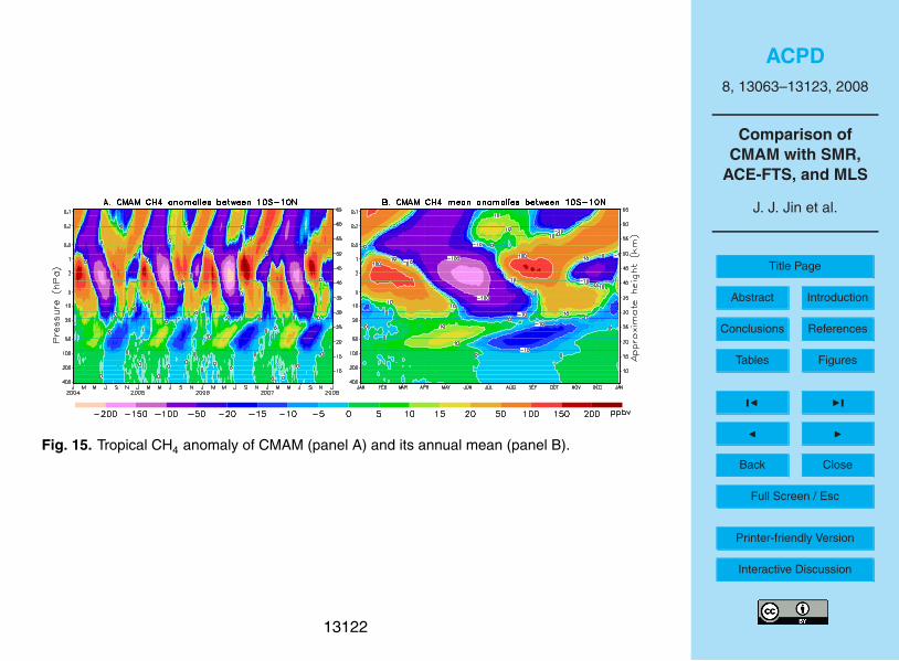
ACPD8, 13063–13123, 2008


ACE-FTS, and MLS

J. J. Jin et al.

Title Page



Tables Figures

J I

J I

Back Close

Full Screen / Esc



Fig. 15. Tropical CH4 anomaly of CMAM (panel A) and its annual mean (panel B).

13122





ACPD8, 13063–13123, 2008


ACE-FTS, and MLS

J. J. Jin et al.

Title Page



Tables Figures

J I

J I

Back Close

Full Screen / Esc


Interactive DiscussionFig. 16. Tropical N2O mean anomalies of SMR (panel A), MLS (panel B) and CMAM (panel C).Panels D, E and F show the anomalies over long-term (periods shown in the plots) averages.

13123





Comparison of CMAM simulations of carbon monoxide (CO), nitrous oxide (N2O), and methane (CH4) with...

Documents

Transcript of Comparison of CMAM simulations of carbon monoxide (CO), nitrous oxide (N2O), and methane (CH4) with...