Clustering high dimensional data using subspace and projected clustering algorithms
Upload
independentCategory
view
2download
0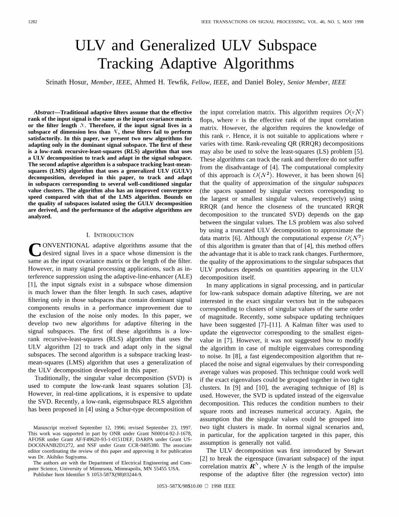
1282 IEEE TRANSACTIONS ON SIGNAL PROCESSING, VOL. 46, NO. 5, MAY 1998
ULV and Generalized ULV SubspaceTracking Adaptive Algorithms
Srinath Hosur,Member, IEEE, Ahmed H. Tewfik,Fellow, IEEE, and Daniel Boley,Senior Member, IEEE
Abstract—Traditional adaptive filters assume that the effectiverank of the input signal is the same as the input covariance matrixor the filter length N: Therefore, if the input signal lives in asubspace of dimension less thanN , these filters fail to performsatisfactorily. In this paper, we present two new algorithms foradapting only in the dominant signal subspace. The first of theseis a low-rank recursive-least-squares (RLS) algorithm that usesa ULV decomposition to track and adapt in the signal subspace.The second adaptive algorithm is a subspace tracking least-mean-squares (LMS) algorithm that uses a generalized ULV (GULV)decomposition, developed in this paper, to track and adaptin subspaces corresponding to several well-conditioned singularvalue clusters. The algorithm also has an improved convergencespeed compared with that of the LMS algorithm. Bounds onthe quality of subspaces isolated using the GULV decompositionare derived, and the performance of the adaptive algorithms areanalyzed.
I. INTRODUCTION
CONVENTIONAL adaptive algorithms assume that thedesired signal lives in a space whose dimension is the
same as the input covariance matrix or the length of the filter.However, in many signal processing applications, such as in-terference suppression using the adaptive-line-enhancer (ALE)[1], the input signals exist in a subspace whose dimensionis much lower than the filter length. In such cases, adaptivefiltering only in those subspaces that contain dominant signalcomponents results in a performance improvement due tothe exclusion of the noise only modes. In this paper, wedevelop two new algorithms for adaptive filtering in thesignal subspaces. The first of these algorithms is a low-rank recursive-least-squares (RLS) algorithm that uses theULV algorithm [2] to track and adapt only in the signalsubspaces. The second algorithm is a subspace tracking least-mean-squares (LMS) algorithm that uses a generalization ofthe ULV decomposition developed in this paper.
Traditionally, the singular value decomposition (SVD) isused to compute the low-rank least squares solution [3].However, in real-time applications, it is expensive to updatethe SVD. Recently, a low-rank, eigensubspace RLS algorithmhas been proposed in [4] using a Schur-type decomposition of
Manuscript received September 12, 1996; revised September 23, 1997.This work was supported in part by ONR under Grant N00014-92-J-1678,AFOSR under Grant AF/F49620-93-1-0151DEF, DARPA under Grant US-DOC6NANB2D1272, and NSF under Grant CCR-9405380. The associateeditor coordinating the review of this paper and approving it for publicationwas Dr. Akihiko Sugiyama.
The authors are with the Department of Electrical Engineering and Com-puter Science, University of Minnesota, Minneapolis, MN 55455 USA.
Publisher Item Identifier S 1053-587X(98)03244-9.
the input correlation matrix. This algorithm requiresflops, where is the effective rank of the input correlationmatrix. However, the algorithm requires the knowledge ofthis rank Hence, it is not suitable to applications wherevaries with time. Rank-revealing QR (RRQR) decompositionsmay also be used to solve the least-squares (LS) problem [5].These algorithms can track the rank and therefore do not sufferfrom the disadvantage of [4]. The computational complexityof this approach is However, it has been shown [6]that the quality of approximation of thesingular subspaces(the spaces spanned by singular vectors corresponding tothe largest or smallest singular values, respectively) usingRRQR (and hence the closeness of the truncated RRQRdecomposition to the truncated SVD) depends on the gapbetween the singular values. The LS problem was also solvedby using a truncated ULV decomposition to approximate thedata matrix [6]. Although the computational expenseof this algorithm is greater than that of [4], this method offersthe advantage that it is able to track rank changes. Furthermore,the quality of the approximations to the singular subspaces thatULV produces depends on quantities appearing in the ULVdecomposition itself.
In many applications in signal processing, and in particularfor low-rank subspace domain adaptive filtering, we are notinterested in the exact singular vectors but in the subspacescorresponding to clusters of singular values of the same orderof magnitude. Recently, some subspace updating techniqueshave been suggested [7]–[11]. A Kalman filter was used toupdate the eigenvector corresponding to the smallest eigen-value in [7]. However, it was not suggested how to modifythe algorithm in case of multiple eigenvalues correspondingto noise. In [8], a fast eigendecomposition algorithm that re-placed the noise and signal eigenvalues by their correspondingaverage values was proposed. This technique could work wellif the exact eigenvalues could be grouped together in two tightclusters. In [9] and [10], the averaging technique of [8] isused. However, the SVD is updated instead of the eigenvaluedecomposition. This reduces the condition numbers to theirsquare roots and increases numerical accuracy. Again, theassumption that the singular values could be grouped intotwo tight clusters is made. In normal signal scenarios and,in particular, for the application targeted in this paper, thisassumption is generally not valid.
The ULV decomposition was first introduced by Stewart[2] to break the eigenspace (invariant subspace) of the inputcorrelation matrix , where is the length of the impulseresponse of the adaptive filter (the regression vector) into
1053–587X/98$10.00 1998 IEEE
HOSUR et al.: ULV AND GENERALIZED ULV SUBSPACE TRACKING ADAPTIVE ALGORITHMS 1283
two subspaces: one corresponding to the cluster of largestsingular values and the other corresponding to the smallersingular values or noise subspace. This method is easilyupdated when new data arrives without making anya prioriassumptions about the overall distribution of the singularvalues. Each ULV update requires only operations. Ananalysis of the ULV algorithm was also performed [6], [12].It was shown in [6] that the “noise” subspace (the subspacecorresponding to the cluster of small singular values) is closeto the corresponding SVD subspace. The analysis of [12] alsoshows that the ULV subspaces are only slightly more sensitiveto perturbations. These analyses show that the ULV algorithmcan be used in many situations where SVD was the onlyavailable alternative to date.
We use the ULV decomposition to develop a low-rankrecursive-least-squares (RLS) algorithm. The proposed algo-rithm tracks the subspace that contains the signal of interestusing the ULV decomposition and adapts only in that subspace.Although the ULV decomposition requires flops, theincrease in computational complexity can be justified by thefact that the ULV decomposition is able to track changes inthe numerical rank.
We also develop a new subspace tracking least-mean-squares (LMS) algorithm. The ULV decomposition tracks onlytwo subspaces: the dominant signal subspace and the smallersingular value subspace. Even though the dominant subspacecontains strong signal components, its condition number mightstill be large. Now, recall that the convergence speed of theLMS algorithm depends inversely on the condition number ofthe input autocorrelation matrix (the ratio of its maximum tominimum eigenvalue) [1], [13]. Thus, a low-rank LMS algo-rithm that uses the ULV decomposition would still have a poorconvergence performance. We therefore develop a generaliza-tion of the ULV algorithm to track several well-conditionedsubspaces of the input correlation matrix. The input is then pro-jected onto these subspaces, and LMS adaptive filtering is per-formed in these well-conditioned subspaces. This improves theconvergence speed of the subspace tracking LMS algorithm.
This paper is organized as follows. In Section II, we describethe rank-revealing ULV decomposition to track subspacescorresponding to clusters of singular values fast and presentvarious heuristics for locating gaps among the singular values.We also discuss the distance between the subspaces obtainedusing the ULV decomposition on a perturbed data matrix andthe true subspaces obtained using an SVD of the unperturbeddata matrix. In Section III, we describe how the ULV leads to aULV-RLS algorithm and analyze the resulting performance inSection IV. In Section V, we propose the GULV algorithm andpresent some results on the quality of the resulting individualsubspaces. Section VI introduces the idea of subspace domainLMS adaptive filtering, and Section VII analyzes its perfor-mance. Numerical examples are discussed in Section VIII.
II. THE ULV DECOMPOSITION
Many signal processing problems require that we isolate thesmallest singular values of a matrix. The matrix is typicallya covariance matrix or a data matrix that is used to estimate
a covariance matrix. The decision as to how many singularvalues to isolate is usually based on a threshold value (find allthe singular values below the threshold) or on a count (find thelast singular values). While extracting the singular values, weoften wants to keep clusters of the singular values together asa unit. In the SVD, this extraction is easy since all the singularvalues are “displayed.” We can, therefore, easily traverse theentire sequence of singular values to isolate the desired set.Therefore, in order to isolate the smallest singular values, weneed to choose a proper threshold and identify all the singularvalues that lie below this threshold. As mentioned earlier, thedrawback of the SVD is that it requires flops. Here,we review the ULV decomposition of Stewart [2]. The ULVdecomposition can be used to divide the singular values intotwo groups and compute a basis for the space spanned by thecorresponding groups of singular vectors.
A. Data Structure
The ULV decomposition of a real matrix (whereis a triple of three matrices , plus a rank
index , where
(2.1)
orthogonal matrix;lower triangular matrix;
has the same shape aswith orthonormal columns.
The lower triangular matrix can be partitioned as
(2.2)
where , which is the leading part of , has a Frobeniusnorm approximately equal to the norm of a vector of theleading singular values of That is, if the singular valuesof satisfy
(2.3)
then This implies thatencapsulates the “large” singular values of, and(the trailing rows of ) approximately encapsulate the
smallest singular values. The last columns ofencapsulate the corresponding trailing right singular vectors.
In the data structure actually used for computation,isneeded to determine the rank index at each stage as newrows are appended. However, is not needed to obtain theright singular vectors. Therefore, a given ULV decompositioncan be represented just by the triple The ULVdecomposition isrank revealing1 in the sense that the norm ofthe matrix is smaller than some specified tolerance.
Thus, this decomposition immediately provides us with thesubspaces corresponding to a group of largest singular valuesand another corresponding to the group of smallest singularvalues.
The ULV updating procedure updates the ULV decomposi-tion of the data matrix corresponding to the input process, as
1This term was coined by T. F. Chan.
1284 IEEE TRANSACTIONS ON SIGNAL PROCESSING, VOL. 46, NO. 5, MAY 1998
Fig. 1. Sketch ofAbsorb One procedure. Upper case letters denote large entries, lower case letters small entries in the ULV partitioning,R denotesan entry of the new row,+ a temporary fill, and� a zero entry.
additional data vectors become available. In essence, it updatesthe subspaces corresponding to the group of large eigenvaluesand that of small eigenvalues of the correlation matrix of theinput to the adaptive filter.
B. Primitive Procedures
The ULV updating process consists of five primitive proce-dures. The first three procedures are designed to allow easyupdating of the ULV decomposition as new rows are appended.Each basic procedure costs operations and consists ofa sequence of plane (Givens) rotations [3]. Premultiplicationby a plane rotation operates on the rows of the matrix,whereas postmultiplication operates on its columns. By usinga sequence of such rotations in a very special order, we canannihilate desired entries while filling in as few zero entries aspossible. We then restore the few zeroes that are filled in. Weshow the operations on, partitioned as in (2.2). Each rotationapplied from the right is also accumulated in to maintainthe identity , where is not saved. The last twoprocedures use the first three to complete a ULV update. Thefive primitive procedures are summarized below.
Augment matrix by one row, yielding
Update matrices to restore the ULV structure.Increment the rank index by 1.
Extract ( )a) an approximation to the last singular value
of (the leading part ofb) an approximation to the left singular vector
of corresponding to this singular value.
Apply transformations to isolate the smallestsingular value of using item (b) from
Decrement the rank index by 1.
Check if there is a gap between item (a) fromand
If yes, this procedure terminates with no furtherprocessing.If no, apply and thenand repeat.
Apply to incorporate the new row.Apply to the resulting toadjust rank boundaries.
We remark that inAbsorb One, we could potentially avoida call to Deflate One by checking whether the rank hasreally increased by one, as suggested in [2]. However, whenincorporated in the generalized ULV process to be described,some calls toDeflate One will still be necessary; therefore,for simplicity, we omit this feature.
1) Choice of Heuristics for Deflation:Various heuristicscan be used to decide if a gap exists in the singular values.The choice of the heuristic is extremely important as it isused to cluster the singular values and, hence, obtain thecorrect singular subspaces. To our knowledge, three heuristics(including the one used in this paper) have been proposedin literature.
The heuristic proposed in [15] estimates the smallest singu-lar value of and compares it with a user specified tolerance.This tolerance, which is provided by the user, is usually basedon some knowledge of the eigenvalue distribution. The choiceof the tolerance is important. If it is too large, the rank may beunderestimated, and if it is too small, it may be overestimated.In addition, as we shall see later, the user has to provide severaltolerances to track more than two clusters using the generalizedULV decomposition. In practice, all these tolerances may notbe available. Therefore, this heuristic cannot be used in theGULV algorithm that we describe next.
A second heuristic has been proposed in [11]. This heuristicdecides that a gap in the singular values exists if
, where is the Frobenius norm of the trailing partThe parameter, which is calledZero Tolerance ,
is selected by the user. It is included to allow for roundoffor other errors. This heuristic has the nice feature that onlythe Spread and the Zero Tolerance need to bespecified. The algorithm then uses this heuristic to clusterall singular values of similar order of magnitude. However,
HOSUR et al.: ULV AND GENERALIZED ULV SUBSPACE TRACKING ADAPTIVE ALGORITHMS 1285
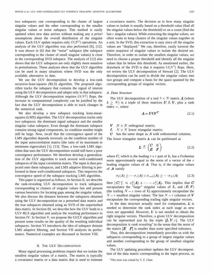
Fig. 2. Tracking performance of ULV using different heuristics for findinga gap in singular values.
when the algorithm initially underestimates the numerical rank,this heuristic leads to some problems. In particular, if oneof the larger singular values lies within the trailing part, theheuristic might decide that no gap exists. Deflation is thenrepeatedly applied till the rank index becomes zero. As thealgorithm is limited to growing the rank boundary by nomore than one for each iteration, the algorithm has to bereinitialized by artificially moving the rank boundary all theway down to the smallest eigenvalue ofand searching forthe rank boundary (using deflations). Fig. 2 shows the ranktracking behavior of the ULV algorithm using the heuristicsof [2] and [11] and that proposed in this paper. The inputinitially consisted of two complex sinusoids, each having anamplitude of 0.1. The background noise was white with avariance of Therefore, there are initially two largesingular values with magnitudes on the order of 0.01 each.The ULV algorithms using all the heuristics converge to a rankestimate of two. Next, a complex exponential of unit amplitudeis added to the input. Now, the larger group of singular valuesis The figure shows that after some time, theULV algorithm using the proposed heuristic and that of [2]converged to a rank of three. However, the ULV algorithmusing the heuristic of [11] converges to one. This is becausethe heuristic initially under estimated the rank as two. Thus,a singular value of magnitude 0.01 is isolated into the trailingpart of , making the Frobenius norm of this part of the sameorder as the smallest singular value of the leading part andforcing a deflation.
The heuristic proposed in this paper tries to combine theadvantages of the two heuristics that we discussed above. Byusing the heuristic proposed in this paper, we can automaticallyisolate clusters of singular values of similar order of magni-tude, i.e., the condition number of each cluster lies within theuser definedSpread . In addition, it does not suffer from thedisadvantage of the second heuristic. If the estimate of the rankboundary is too low, the heuristic allows the rank to grow untilit attains the correct value. This heuristic estimates the smallestsingular value of in addition to that of The heuristic
then decides that a gap between the singular values exists if, where is theSpread chosen by the user. Thus, this
heuristic does not require a user-specified tolerance. In caseof the GULV decomposition, is simply the smallest value ofthe small singular value group adjacent to the group on whichDeflate To Gap is being applied. We shall see later thatthis heuristic can be used with the GULV decomposition withminimum additional computations. The tracking performanceof the ULV decomposition using this heuristic is shown in Fig.2. Note that if we replace by the user-specified tolerancein our heuristic, we obtain the heuristic of [2].
C. Quality of Subspaces
Let be a subspace with orthonormal basis (a matrixwith orthonormal columns), let be the orthogonalprojector onto that subspace, and let be an orthonormalbasis for (the orthogonal complement to). Let bea second subspace of dimension equal to that ofwithcorresponding quantities The distance between thesubspaces is characterized by the sine of the angle betweenthem [3, p. 76]
(2.4)
Bounds have been derived for the ULV algorithm to assess thedistance between the ULV subspaces and the correspondingsingular subspaces and to measure sensitivity of the subspacesto perturbations.
Let the ULV decomposition of and a perturbedbe represented as
a and
b (2.5)
and let the SVD of be given by
(2.6)
Furthermore, let denote the column space of matrix(the subspace spanned by the columns of). The followingtheorem due to Fierro and Bunch [6] shows that as the off-diagonal block decreases, the ULV subspaces converge totheir SVD counterparts.
Theorem 1 (Fierro and Bunch):Let have the ULV in(2.5a) and the SVD in (2.6). Assume that
1286 IEEE TRANSACTIONS ON SIGNAL PROCESSING, VOL. 46, NO. 5, MAY 1998
If , then
These bounds also reveal that there is a limit on how closesome subspaces can be.
In most applications, we will have access to the perturbedmatrix rather than itself. Let have theULV decomposition (2.5b). Further, let and form anorthogonal basis for and , respectively. Define
(2.7)
Then, the following theorem bounds the sensitivity of the ULVsubspaces.
Theorem 2 (Fierro): Let and have the ULV decompo-sitions (2.5). If then for as defined in(2.7), we have
These results indicate that the ULV subspaces are only slightlymore sensitive to perturbations than the singular subspaces[12].
The above theorems provide us with bounds on the distancebetween ULV subspaces and the SVD subspaces of a givenmatrix as well as bounds on the effect on the ULV spaceswhen the matrix is perturbed. However, what if the two effectsare combined? This is relevant because the theory behind theperformance of many signal processing algorithms dependson the exact SVD derived from the “exact” signal, but weare computing the cheaper ULV of a signal subject to noiseand round-off error. Such combined bounds may be obtaineddirectly from Theorem 2 by noting that the SVD ofmay beviewed as a ULV decomposition with
, and Hence, we have the following newtheorem.
Theorem 3: Let and have the SVD and ULV decom-positions (2.6) and (2.5b), respectively. If ,then for as defined in (2.7), we have
The above theorem indicates that as the norm of the off-diagonal block decreases, the error between the ULVsubspace and the corresponding true SVD subspace is domi-nated by the magnitude of the perturbation in the data matrix.
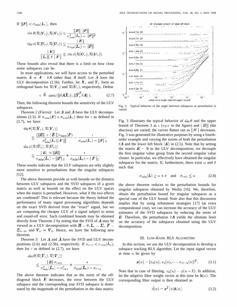
Fig. 3. Typical behavior of the angle between subspaces as perturbation isvaried.
Fig. 3 illustrates the typical behavior of and the upperbound of Theorem 3 as (eps in the figure) and (theabscissa) are varied; the curves flatten out as decreases.Fig. 3 was generated for illustrative purposes by using a fourth-order example and varying the norms of both the perturbation
and the lower left block in (2.5). Note that by settingthe matrix in the ULV decomposition, we decouplethe first singular value group from the second singular valuecluster. In particular, we effectively have obtained the singularsubspaces for the matrix. If, furthermore, there existandsuch that
and (2.8)
the above theorem reduces to the perturbation bounds forsingular subspaces obtained by Wedin [16]. We, therefore,obtain the perturbation bound for singular subspaces as aspecial case of the ULV bound. Note also that this discussionimplies that by using refinement strategies [17] (at extracomputational cost), we can increase the accuracy of the ULVestimates of the SVD subspaces by reducing the norm of
Therefore, the perturbation yields the ultimate limiton the accuracy of the subspaces obtained using the ULVdecomposition.
III. L OW-RANK RLS ALGORITHM
In this section, we use the ULV decomposition to develop asubspace tracking RLS algorithm. Let the input signal vectorat time be given by
(3.1)
Note that in case of filtering, In addition,let the adaptive filter weight vector at this time be Thecorresponding filter output is then obtained as
(3.2)
HOSUR et al.: ULV AND GENERALIZED ULV SUBSPACE TRACKING ADAPTIVE ALGORITHMS 1287
The error between the desired response and that estimatedby the adaptive filter can be written as
(3.3)
The RLS algorithm tries to recursively solve the weighted LSproblem
(3.4)
By rewriting (3.4), we find that the RLS algorithm solves thefollowing problem [1]:
(3.5)
In (3.5), is the desired responsevector, is the input data matrix given by
(3.6)
and is the diagonal exponential weighting matrixgiven by
(3.7)
When , the LS solution can be expressed in terms ofthe SVD as
(3.8)
Here, denotes the pseudoinverse [3].When is close to rank deficient, the least squares
solution is ill conditioned due to the inversion of the smallsingular values in In such cases, a rankapproximant
of the matrix is constructed by setting thesmall singular values of to zero in its singular valuedecomposition. Thus, if the singular value decomposition of
is given by (2.6), its low rank approximate is given by
(3.9)
The solution to the modified LS problem is then obtained as
(3.10)It has been recently suggested [18] that the rankapproximateof , which was discussed above, be replaced by a matrixobtained using a truncated ULV decomposition. The mainmotivations behind the use of the ULV decomposition is itslower computational expense as compared with theSVD Thus, the ULV-LS solution (an approximationto the “exact” MLS solution) can be computed as [18]
- (3.11)
It was, however, not suggested how the algorithm is to bemodified in case the data matrix grows as new databecomes available. Clearly, in such a case, storing is
not a viable option. In this section, we suggest a method toobtain a recursive solution to the modified LS problem (3.10).
The LS minimization problem discussed above is invariantunder any unitary transformation. For some , let theULV decomposition of the weighted data matrix be given as
(3.12)
where the columns of and can again be clusteredas in (2.5). Then
(3.13)
where
(3.14)
Thus, the RLS problem is equivalent to solving, for , thesystem of linear equations
(3.15)
Note that Therefore, the above equa-tion can be rewritten as
(3.16)
where are the first elements of Thus, the low-rank RLS solution can be obtained in two steps as
a and
b - (3.17)
The computation of the ULV-LS solution using (3.17) a) andb) requires only flops.
Note that the ULV algorithm updates andfrom previously computed values. To do this, it appends thenew input vector as a row to and appliesGivens rotations from the right and the left in a special orderto compute This operation can be written as
(3.18)
The ULV algorithm discards all the rotations applied from theleft. The right rotations are absorbed into However, thevector can be easily updated from as
(3.19)
Since each Givens rotation affects only two elements of thevector, we must perform flops to update Thus,the low-rank RLS requires flops per iteration.
1288 IEEE TRANSACTIONS ON SIGNAL PROCESSING, VOL. 46, NO. 5, MAY 1998
IV. ULV-RLS PERFORMANCE ANALYSIS
In this section, we perform a simple convergence analysis ofthe ULV-RLS algorithm. The ULV subspaces are, in general,perturbed from their SVD counterparts. Therefore, the mainpurpose of this section is to analyze these effects on theconvergence behavior of the ULV-RLS algorithm. For therest of this section, we assume that the algorithm operatesin a stationary environment. Therefore, we set the exponentialweighting factor to get the optimal steady-state result.This assumption implies that the environment is stationaryand allows us to draw some general conclusions about theULV-RLS algorithm.
In order to analyze the behavior of the ULV-RLS algorithm,we consider the following multiple linear regression model.Assume that the input is in a low-rank subspace of dimension, where The input vector at time
is projected into the -dimensional subspace using atransformation matrix The columns of are theeigenvectors of the covariance matrixcorresponding to its nonzero eigenvalues. The resultingvector is weighted by , which is anregression parameter vectorin the transform domain. Thedesired output is then generated, according to this model,as
(4.20)
where is called themeasurement error, and is thecorresponding time domain regression parameter vector
(4.21)
The process is assumed to be white with zero meanand variance Since the algorithm operates in a stationaryenvironment, the vector is constant.
A. Weight Vector Behavior
The rank- ULV-RLS weight vector at time -satisfies [see (3.11)]
- (4.22)
From (4.20), we see that the regression vector satisfies
(4.23)
where is the vector of themeasurement errors up to timeAs the rank of is , wecan rewrite (4.23) using the SVD of defined in (2.6), as
(4.24)
Subtracting (4.24) from (4.22), multiplying both sides of theresult by , and performing some simple mathematicalmanipulations, we obtain
-
(4.25)
Notice that is an approxi-mation to the matrix, Therefore
or (4.26)
(4.27)
where is the error in the approximation. Thus, from(4.25) and (4.27), we obtain
- (4.28)
Taking the expectation of both sides of (4.28) for a givenrealization and noting that the measurementerror has zero mean, we obtain
- (4.29)
Assuming the stochastic process represented by is er-godic, we can approximate the ensemble averaged covariancematrix of as
large (4.30)
Thus, (4.29) can be rewritten as
-
(4.31)
In the above expression, astends to infinity, the perturbationtends to a finite value due to the inaccuracy in the
subspaces estimated by the ULV decomposition. In fact, it hasbeen shown that [18]
(4.32)
Thus, unlike the traditional RLS algorithm, which is asymptot-ically unbiased [1], the ULV-RLS algorithm has a small bias.However, the magnitude of this bias depends on the closenessof the ULV subspace to its corresponding singular sub-
HOSUR et al.: ULV AND GENERALIZED ULV SUBSPACE TRACKING ADAPTIVE ALGORITHMS 1289
space. This closeness, in turn, depends on the magnitude ofthe off-diagonal matrix (see Theorem 1). Therefore, usingextra refinements [17], it is possible to reduce the norm ofto close to zero (i.e., extra refinements will make the matrix
close to block diagonal) and make the bias negligible.
B. Mean Squared Error
Let us now perform a convergence analysis of the RLSalgorithm based on the mean squared value of thea prioriestimation error of the RLS algorithm.
The a priori estimation error is given by
- (4.33)
Eliminating between (4.33) and (4.20), we obtain
-(4.34)
We now note that it follows from (4.28) that
(4.35)
Define We then have
(4.36)
(4.37)
where we used the fact that is independent ofgiven
We therefore have
(4.38)
Notice that the second term in the above equation dependson the distance between the ULV and the SVD subspaces.Now, the magnitude of depends on the norm of
the off diagonal matrix (see [18], (4.32), and Theorem1). This norm can be made arbitrarily small using extrarefinements [17]. Furthermore,the magnitude of the third termin the right-hand side of (4.38) is Therefore, for smallperturbations, thea priori MSE is
(4.39)
If we now take the expectation of both sides of the aboveequation with respect to and use (4.30) and the definitionof , we obtain for large
(4.40)
Based on (4.40), we can make the following observationsabout the ULV-RLS algorithm: 1) The ULV-RLS algorithmconverges in the mean square in about iterations,i.e., its rate of convergence is of the same order as thatof the traditional RLS algorithm, and 2) if the quality ofthe subspaces approximated are high, e.g., in a stationaryenvironment, thea priori MSE of the ULV-RLS approachesthe variance of the measurement error. Therefore, in theory, insuch an environment, it has a zero excess MSE. Thus, its MSEperformance is similar to that of the traditional RLS algorithm.
V. GENERALIZED ULV UPDATE
As mentioned in the Introduction, the ULV decompositiontracks only two subspaces: the dominant signal subspace andthe smaller singular subspace. Even though the dominant sub-space contains strong signal components, its condition numbermight still be large. Thus, a low-rank LMS algorithm that usesthe ULV decomposition would still have a poor convergenceperformance. We therefore generalize the ULV decompositionin this section to track subspaces corresponding to more thantwo clusters of singular values. The GULV decompositionis represented by the “tuple” , whereare defined as in (2.1), and the’s are integer-valued rankboundaries such that each of the triplesis an ordinary ULV decomposition. This means that the first
rows of encapsulates the first singular values offor For example, the GULV decomposition for
has the form
(5.1)
wherehave columns, respectively, being partitionedconformally.
1290 IEEE TRANSACTIONS ON SIGNAL PROCESSING, VOL. 46, NO. 5, MAY 1998
Each update in the GULV decomposition consists of ap-pending a row and restoring the lower triangular structure of
followed by an adjustment of all the rank indicesto restore the separation between each cluster. This task isaccomplished by using the primitive operations from SectionII-B. The following is a sketch of the procedures in a formsuitable for exposition, although the specific implementationcould be reorganized for efficiency.
Apply to with the new row(incrementing ).
Increment by 1, for
Apply to is decremented).For increment by 1.If apply to
(recursively).(
Check if would deflate
If yes, apply toand repeat.
If not, this procedure terminates with no furtherprocessing.
Apply to incorporate thenew row.
Apply toto adjust rank boundaries.
A. Quality of Subspaces
The theory of Section II-C can be used to boundthe distance between the spaces
arising from the GULV (5.1) and thecorresponding true singular subspaces that would arise fromthe true SVD. Here, we show that the results of Section II-Calso provide a bound on the distances between the individualGULV subspaces , etc. and their correspondingtrue singular subspaces. Specifically, we have the followingtheorem.
Theorem 4: Consider two orthogonal matricesand Define the upper
bounds for each
Then, we have the following bounds between the individualblock columns:
(5.2)
Proof: We illustrate the proof for the case ; thegeneral case is similar. We have the orthogonal matrices
andThe distances between the subspaces can be analyzed usingthe product
(5.3)
By (2.4), the distance between and is
We observe that
from which it follows that (5.2) must hold for The casefor general and general is handled similarly.
Applying this result to the matrix in the GULV decom-position, the theory of Section II-C shows that the perturbedsubspaces spanned by converges to the true leadingsingular subspace as the off-diagonal entries decrease to zero.Hence, (5.2) shows that each individual block of columnsalso converges to the correspondingth individual singularsubspace.
VI. GENERALIZED ULV-LMS A LGORITHM
The LMS algorithm tries to minimize the mean squaredvalue of the error given by (3.3) by updating the weightvector with each new data sample received as
(6.1)
where the step size is a positive constant.As noted in the Introduction, the convergence of the LMS al-
gorithm depends on the condition number of the input autocor-
relation matrix [1], [19], whereWhen all the eigenvalues of the input correlation matrix areequal, i.e., the condition number , the algorithmconverges fastest. As the condition number increases (i.e., asthe eigenvalue spread increases or the input correlation matrixbecomes more ill conditioned), the algorithm converges moreslowly.
Instead of using a Newton-LMS or a transform domainLMS algorithm to improve the convergence speed of theLMS algorithm, we will develop here a GULV-based LMSprocedure. The GULV decomposition groups the singularvalues of any matrix into an arbitrary number of groups. Thenumber of groups or clusters is determined automatically bythe largest condition number that can be tolerated in eachcluster. This condition number in turn is determined by each
HOSUR et al.: ULV AND GENERALIZED ULV SUBSPACE TRACKING ADAPTIVE ALGORITHMS 1291
cluster that has singular values of nearly the same orderof magnitude, i.e., the condition number in each cluster isimproved. If we now apply an LMS algorithm to a projectionof the filter weights in each subspace, the projected weightswill have faster convergence. The convergence of the overalladaptive procedure will depend on the most ill-conditionedsubspace, i.e., the maximum of the ratio of the largest singularvalue in each cluster to its smallest singular value.
Let us transform the input using the unitary matrixobtained by the GULV decomposition. As the GULV decom-position is updated at relatively low cost, this would implya savings in the computational expense. We note thatalmost block diagonalizes in the sense that it exactly blockdiagonalizes a small perturbation of it. In particular, let theinput data matrix withdefined by (2.2). Since exactly blockdiagonalizes as
where
Here, is small, withLet the input data vector be transformed using as
(6.2)
The first coefficients of belong to the subspacecorresponding to the first singular value cluster, the nextcoefficients to the second singular value cluster, and so on.The variance of coefficients of in each such cluster isnearly the same. This is due to the fact that each subspaceis selected to cluster the singular values to minimize thecondition number in that subspace. This implies that theadaptive filter coefficients in the transform domain can alsobe similarly clustered.
The GULV-LMS update equations for updating the trans-form domain adaptive filter vector are given as
a and
b (6.3)
where is a diagonal matrix of step sizes used, andis an orthogonal matrix indicating the cumulative effect ofGivens rotations performed to update from ,i.e.,
(6.4)
It is easy to deduce from the fact that the output of thetransform domain adaptive filter should be the same as thatof the tapped delay line adaptive filter that
(6.5)
and
(6.6)
As the transformed coefficients belonging to a single clusterhave nearly the same variance, the corresponding coefficientsof can be adapted using the same step size. In otherwords, the diagonal elements of are clustered into valuesof equal step sizes
diag (6.7)
The size of each cluster matches the dimension of the cor-responding subspace. The adaptation within each subspacetherefore has nearly optimal convergence speed. Thus, forthe subspace tracking LMS filter to have a fast convergence,it should converge with the same speed in each subspace.This implies that the slow converging subspace projections(usually the ones with lower signal energy) should be assignedlarge step sizes. Note that the average time constantofthe learning curve [1] is , where isthe average eigenvalue of the input correlation matrix or theaverage input power. Therefore, the step size for coefficientsin a subspace should be made inversely proportional to theaverage energy in that subspace. Now, note that the diagonalvalues of the lower triangular matrix generated by theGULV decomposition reflect the average magnitude of thesingular values in each cluster. This information can thereforebe directly used to select the step sizes.
As the slowly converging subspace projections are usuallythose subspaces with lower signal energy, a large step size forthese subspaces implies that the noise in these subspaces isboosted. By not adapting in these subspaces, we can reducethe excess MSE. This can be done by setting the correspondingdiagonal entries of to zero. In addition, in case theautocorrelation matrix is close to singular, the projectionsof the tap weights onto the subspaces corresponding to zerosingular values need not be updated. This results in stableadaptation.
VII. GULV-LMS PERFORMANCE ANALYSIS
Several analyzes of the LMS and Newton-LMS algorithmhave appeared in literature. The GULV-LMS algorithm differsfrom traditional LMS and Newton-LMS type algorithms inthat the subspaces estimated by the GULV algorithm areperturbed from the true subspaces by a small amount. Thegoal of this section is to analyze the effect of this perturbationon the performance of the algorithm. Specifically, we willconsider its effect on the mean and mean-squared behaviorof the weight vectors in our algorithm. We also study itseffect on the steady-state mean square error of the proposedalgorithm. Our analyses are approximate in that they relyon the standard simplifying assumptions that have been usedin the literature to analyze the various variants of the LMSalgorithm. They nevertheless provide guidelines for selecting
and an understanding of the performance of the algorithmsthat is confirmed by simulations (cf. Section VIII). Therefore,we make the following standard assumptions to simplify theanalysis:
1) Each sample vector is statistically independent ofall previous vectors
(7.1)
1292 IEEE TRANSACTIONS ON SIGNAL PROCESSING, VOL. 46, NO. 5, MAY 1998
2) Each sample vector is statistically independent ofall previous samples of the desired response
(7.2)
3) The desired response at theth instance dependson the corresponding input vector
4) The desired response and the input vector arejointly Gaussian.
A. Weight Vector Behavior
Based on these assumptions, we can show that the GULV-LMS algorithm will converge with sufficiently small stepsizes
Specifically, let be the th eigenvalue of the inputcovariance matrix , and let be the perturbation to theeffective covariance matrix arising from the fact that theGULV does not yield the exact subspaces. Then, we showin Appendix A that for convergence, it is sufficient to choose
as
(7.3)
B. Mean Squared Error
The MSE of the LMS algorithm is given by
(7.4)
This equation can be rewritten in terms of the weight errorvector as [1]
(7.5)
In the above equation, denotes the minimum MSEachieved by the optimum weight vector. The excess MSE isthen given by
Tr (7.6)
where Tr denotes the trace operator, andis the weight error correlation matrix. The
misadjustment error is the excess MSE after the adaptive filterhas converged,
One can show that is given by
TrTr
(7.7)
where is the diagonal eigenvalue matrix of the inputcorrelation matrix This can be derived in a straightforwardmanner following the method outlined in [1, Sec. IX-D] (Sec.IX-G in the second edition); therefore, we omit it for brevity.
C. Discussion
The condition on for convergence (7.3) is similar to thatobtained in [19] and [20]. Specifically, when the matrix isreplaced by a multiple of the identity matrix and ,the convergence condition becomes
(7.8)
Note also that if the subspaces estimated using the GULValgorithm were the true subspaces and the condition numberof each cluster is 1, then , and by choosing such that
(7.9)
the convergence condition becomes
(7.10)
This is equivalent to whitening the input process by precon-ditioning with the appropriate In practice, the elementsof are negligible, and is very small. Further, thestep size for each cluster is chosen to be the inverse ofthe estimate of the variance of the component of the inputsignal that lies in the cluster (i.e., the inverse of the average ofthe eigenvalues in the cluster). This implies that the conditionfor convergence (7.3) is almost always satisfied in practice.Choosing the step sizes as the inverse of the estimated powerin each cluster also matches the speeds of adaptation acrossthe clusters.
The step sizes for modes/subspaces that contain essentiallynoise and little signal components can be chosen to be verysmall. As the subspaces have been decoupled on the basisof signal strengths, adapting very slowly or not at all in thenoise only subspaces leads to little loss of information, whichis confirmed by simulations (cf. Section VIII). As discussedin the Appendix, adapting only in thedominant subspacescorresponds to adaptively estimating the solution to the mod-ified Wiener equation (A.6). This implies that there is aninherent “noise cleaning” associated with such an approach. Itis noted [22] that as we slowly increase the number of nonzero
’s corresponding to the subspaces containing significantsignal strengths, the MSE decreases until the desired signalsare contained in these spaces. A further increase would onlyincrease the MSE due to the inclusion of the noise eigenvalues.In addition, note that the solution to the unmodified normal(A.3) involve inverting the input correlation matrix. Therefore,the contribution of the noise eigenvalues to the MSE using thissolution is inversely proportional to their magnitudes. Hence,if the noise eigenvalues are small (high SNR), this amountsto noise boosting, resulting in a larger MSE. As conventionaladaptive filters recursively estimate this solution, their MSEat convergence is also high.
Equations (A.17) and (A.18) give a recursive update equa-tion for the weight error vector. The speed with which thisweight error vector tends to zero determines the speed of con-vergence of the algorithm. Assume that the GULV projectionshave converged at step In addition, assume that we cancluster the eigenvalues of into clusters, i.e., the diagonaleigenvalue matrix of can be written as
......
...(7.11)
where is the diagonal matrix of eigenvalues correspondingto the th cluster. Rewriting (A.18) in terms of some weight

HOSUR et al.: ULV AND GENERALIZED ULV SUBSPACE TRACKING ADAPTIVE ALGORITHMS 1293
error vector , we obtain for
diag
diag (7.12)
For sufficiently small , (7.12) indicates that the conver-gence speed in each subspace depends on the step size matrix
and the condition number of For the same stepsize, the modes corresponding to smaller eigenvalues ofconverge more slowly than those corresponding to its largereigenvalues. In addition, note that to achieve minimum MSE,one needs to adapt only in the signal subspaces. Therefore, theconvergence of the GULV-LMS adaptive filter to the requiredsolution depends only on the condition number of the clusteridentified by the GULV decomposition corresponding to eachof the
For the th subspace identified by the GULV algorithm, thecondition number is given as
th subspace
(7.13)
However, as noted above, in steady state, the perturbation isvery small, and the condition number of the subspace identifiedby the GULV decomposition is close to the condition numberof the corresponding cluster of eigenvalues. The speed ofthe adaptive algorithm therefore depends on the speed ofconvergence in that subspace that has the maximum conditionnumber. By proper application of the GULV algorithm andchoice of the subspaces, this condition number can be madeto be close to unity for fast convergence.
The misadjustment error expression given by (7.7) is ap-proximate. In deriving this result, we have made use of thefact that is a very small perturbation and can be neglected.Now, if the step size for the th dominant cluster is chosensuch that
Tr
where Tr is the total input power in that cluster, then itcan be easily verified that Tr (size of the inputsignal subspace). Thus, for small, the misadjustment errordepends linearly on the step size and the effective rank of theinput signal.
We therefore conclude that for a step size leading to thesame misadjustment error, the GULV-LMS algorithm wouldconverge at least as fast as the LMS algorithm. It wouldconverge faster than the LMS algorithm when the conditionnumber of the input correlation matrix is large.
VIII. SIMULATION RESULTS
An adaptive line enhancer (ALE) experiment was conductedto illustrate the performance of the algorithm when the adap-tation is done only in the signal subspaces. The input to theALE was chosen to beWhite Gaussian noise with a variance of60 and 160 dB
(a)
(b)
Fig. 4. Learning curves illustrating performance. Noise at�60 dB. Curvesare averages of 20 runs.
was added to obtain the learning curves of Figs. 4 and 5,respectively. The figures show the performance of the GULV-LMS algorithm, the plain ULV-LMS, plain LMS, traditionalRLS, QRD-RLS, ULV-RLS, and the Schur pseudoinverse-based least squares method discussed in [4]. The learningcurves show the improved performance of the GULV-LMSalgorithm. It can be seen from these figures that breakingup the subspaces corresponding to the larger singular valuesinto subclusters using the GULV algorithm further reduces thecondition numbers of these clusters. This, in turn, yields animprovement in the convergence performance of the GULV-LMS algorithm.
Fig. 5 also demonstrates the stability of the GULV-basedRLS and LMS algorithms when the input matrix becomesnumerically ill conditioned. As the GULV-based algorithmsare based on Givens rotations, they enjoy the same stabilityproperties of the QRD-RLS algorithm.
Fig. 6 shows the tracking behavior of the GULV-basedprocedures. The input to the ALE in this figure is initially
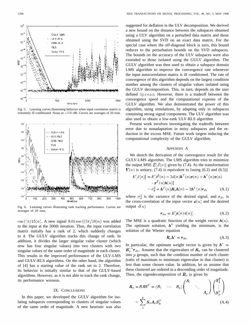
1294 IEEE TRANSACTIONS ON SIGNAL PROCESSING, VOL. 46, NO. 5, MAY 1998
Fig. 5. Learning curves illustrating behavior when input correlation matrix isextremely ill conditioned. Noise at�160 dB. Curves are averages of 20 runs.
Fig. 6. Learning curves illustrating rank tracking performance. Curves areaverages of 20 runs.
A new signal was addedto the input at the 500th iteration. Thus, the input correlationmatrix initially has a rank of 2, which suddenly changesto 4. The GULV algorithm tracks this change of rank. Inaddition, it divides the larger singular value cluster (whichnow has four singular values) into two clusters with twosingular values of the same order of magnitude in each cluster.This results in the improved performance of the ULV-LMSand GULV-RLS algorithms. On the other hand, the algorithmof [4] has a starting value of the rank set to 2. Therefore,its behavior is initially similar to that of the GULV-basedalgorithms. However, as it is not able to track the rank change,its performance worsens.
IX. CONCLUSIONS
In this paper, we developed the GULV algorithm for iso-lating subspaces corresponding to clusters of singular valuesof the same order of magnitude. A new heuristic was also
suggested for deflation in the ULV decomposition. We deriveda new bound on the distance between the subspaces obtainedusing a ULV algorithm on a perturbed data matrix and thoseobtained using the SVD on an exact data matrix. For thespecial case where the off-diagonal block is zero, this boundreduces to the perturbation bounds on the SVD subspaces.The bounds on the accuracy of the ULV subspaces were alsoextended to those isolated using the GULV algorithm. TheGULV algorithm was then used to obtain a subspace domainLMS algorithm to improve the convergence rate wheneverthe input autocorrelation matrix is ill conditioned. The rate ofconvergence of this algorithm depends on the largest conditionnumber among the clusters of singular values isolated usingthe GULV decomposition. This, in turn, depends on the userdefinedSpread . However, there is a tradeoff between theconvergence speed and the computational expense of theGULV algorithm. We also demonstrated the power of thisalgorithm, using simulations, by adapting only in subspacescontaining strong signal components. The ULV algorithm wasalso used to obtain a low-rank ULV-RLS algorithm.
Present work involves investigating the tradeoffs betweenerror due to nonadaptation in noisy subspaces and the re-duction in the excess MSE. Future work targets reducing thecomputational complexity of the GULV algorithm.
APPENDIX A
We sketch the derivation of the convergence result for theGULV-LMS algorithm. The LMS algorithm tries to minimizethe output MSE given by (7.4). As the transformation
is unitary, (7.4) is equivalent to [using (6.2) and (6.5)]
(A.1)
where is the variance of the desired signal, and isthe cross-correlation of the input vector and the desiredoutput
(A.2)
The MSE is a quadratic function of the weight vectorThe optimum solution, yielding the minimum, is thesolution of the Wiener equation
(A.3)
In particular, the optimum weight vector is given byAssume that the eigenvalues of can be clustered
into groups, such that the condition number of each cluster(ratio of maximum to minimum eigenvalue in that cluster) isless than some chosen value. In addition, let us assume thatthese clustered are ordered in a descending order of magnitude.Then, the eigendecomposition of is given by
......
(A.4)
HOSUR et al.: ULV AND GENERALIZED ULV SUBSPACE TRACKING ADAPTIVE ALGORITHMS 1295
where is the number of eigenvalues in theth cluster. Now,consider a low-rank solution to the Wiener equation (A.3).Let the rank low-rank approximate for be the matrixconstructed by replacing the smallest eigenvalue clustersof in its eigendecomposition by zeros, i.e.,
(A.5)
The -order solution is then obtained by solving the mod-ified Wiener equation
(A.6)
for each Note that when In addition,if is the projector onto the subspace spanned by theeigenvectors corresponding to theth cluster, it follows fromthe definition of the projectors that
(A.7)
Suppose now that we use a GULV-LMS algorithm thatadapts only in the dominant subspaces produced by theGULV decomposition. Let be the time domain weightvector that it produces. We now proceed to show that under thesimplifying assumptions listed in Section VII, convergesto with a very small bias. This bias depends on the qualityof the estimated subspaces i.e., how close they are to the trueeigenvector subspaces. We also show that whenconverges to with a zero bias as tends to infinity.
Let the unitary transformation matrix be partitionedinto blocks, each block corresponding to the subspace of acluster eigenvalues having the same order of magnitude
The orthogonal projection matrix in the subspacecorresponding to the th cluster of eigenvalues is obtainedapproximately by the GULV algorithm at theth as
The GULV-LMS update (6.3a) can thereforebe rewritten as
(A.8)
Note that step-size matrix is chosen to be a block diagonalmatrix, with each block being a scalar multiple of the identityof appropriate dimension. This is due to the fact that we havea single step size for the modes belonging to a single clusterof eigenvalues. Premultiplying the above equation by ,we obtain
(A.9)
where denotes the projection of the inputvector onto the subspace estimate corresponding to the
th cluster of eigenvalues.
We define the weight error vector as
(A.10)
where is the modified Wiener solution as discussed above.Subtracting from both sides of (A.9), and using (A.10)
and (3.3), we obtain
(A.11)
From Theorems 2 and 3, it can be seen that the distancebetween the perturbed ULV subspaces and the correspondingtrue subspaces depends on the amount of perturbationTheinput correlation matrix is estimated as a sample average
Therefore, the perturbationtendsto 0 as tends to infinity. This implies that for large, wecan assume that converges to its steady-state value,which is independent of Taking the expectation of bothsides of (A.11), for large , we obtain
(A.12)
where we have made use of the independence assumptions.Noting that
(A.13)
and using (A.3), we obtain
(A.14)
Using (A.4), (A.7), and the fact that and are orthogonalprojections and , it is easy to verify that wheneverthe estimated subspaces converge to the exact subspaces (i.e.,
) or when , the second term in(A.14) is zero.
However, the subspaces estimated by the GULV algorithmwill, in general, be perturbed from the true subspaces by asmall amount. Therefore, we have
a and
b (A.15)
1296 IEEE TRANSACTIONS ON SIGNAL PROCESSING, VOL. 46, NO. 5, MAY 1998
Using (A.15b) in (A.14), the weight error update equation canbe rewritten as
(A.16)
(A.17)
where is the eigendecomposition of Bymaking the transformation and , we canrewrite (A.17) as
(A.18)
where This error equation isof the form derived for the LMS algorithm [1] and can berewritten as
(A.19)
We can now state the main result of this analysis as follows.If the step size for each cluster satisfies the condition [19],[20]
(A.20)
where is the perturbation in the corresponding eigenvaluedue to the perturbation matrix , then the quantities
and go to zero as , andhence, it follows that
(A.21)
This result shows that unlike the LMS algorithm, for theGULV-LMS algorithm, Again, from Theorem3, we can see that if the norm of the off-diagonal matrixisreduced close to zero using refinement strategies, then for large
, the ULV subspaces converge to the true SVD subspaces. Inpractice, the norms and are usually small,or they can be reduced using extra refinements so that thebias is negligible. In addition, as pointed out earlier, for thecase This, in tur,n implies thatTherefore, for , the algorithm converges in mean to theoptimum weight vector
Using the inequality (see Weyl’sTheorem [21, p. 203]), we get the inequality
Thus for convergence, it is sufficient tochoose as
(A.22)
REFERENCES
[1] S. Haykin, Adaptive Filter Theory. Englewood Cliffs, NJ: Prentice-Hall, 3rd ed., 1995.
[2] G. W. Stewart, “An updating algorithm for subspace tracking,”IEEETrans. Signal Processing, vol. 40, pp. 1535–1541, June 1992.
[3] G. H. Golub and C. F. Van Loan,Matrix Computations, 3rd ed.Baltimore, MD, John Hopkins Univ. Press, 1996.
[4] P. Strobach, “Fast recursive eigensubspace adaptive filters,” inProc.ICASSP, 1995, vol. 2, pp. 1416–1419.
[5] T. F. Chan and P. C. Hansen, “Some applications of the rank revealingQR factorization,”SIAM J. Sci. Stat. Comput., vol. 13, pp. 727–741,1992.
[6] R. D. Fierro and J. R. Bunch, “Bounding the subspaces from rankrevealing two-sided orthogonal decompositions,”SIAM J. Matrix Anal.Appl., vol. 16, no. 3, pp. 743–759, 1995.
[7] C. E. Davila, “Recursive total least squares algorithm for adaptivefiltering,” in Proc. ICASSP, May 1991, pp. 1853–1856.
[8] K. B. Yu, “Recursive updating the eigenvalue decomposition of a covari-ance matrix,”IEEE Trans. Signal Processing, vol. 39, pp. 1136–1145,1991.
[9] E. M. Dowling and R. D. DeGroat, “Recursive total least squaresadaptive filtering,” inProc. SPIE Conf. Adaptive Signal Process., vol.1565, pp. 35–46, July 1991.
[10] R. D. DeGroat, “Noniterative subspace tracking,”IEEE Trans. SignalProcessing, vol. 40, pp. 571–577, 1992.
[11] D. L. Boley and K. T. Sutherland, “Recursive total least squares: Analternative to the discrete Kalman filter,” Tech. Rep. TR 93-92, Dept.Comput. Sci., Univ. Minnesota, Minneapolis, 1993.
[12] R. D. Fierro, “Perturbation analysis for two-sided (or complete) orthog-onal decompositions,”SIAM J. Matrix Anal. Appl., vol. 17, no. 2, pp.383–400, 1996.
[13] D. F. Marshall, W. K. Jenkins, and J. J. Murphy, “The use of orthogonaltransforms for improving performance of adaptive filters,”IEEE Trans.Circuits Syst., vol. 36, pp. 474–483, Apr. 1989.
[14] N. J. Higham, “A survey of condition number estimators for triangularmatrices,”SIAM Rev., pp. 575–596, 1987.
[15] G. W. Stewart, “Updating a rank-revealing ULV decomposition,”SIAMJ. Matrix Anal. Appl., vol. 14, pp. 494–499, 1993.
[16] P. A. Wedin, “Perturbation bounds in connection with singular valuedecomposition,”BIT, vol. 12, pp. 99–111, 1973.
[17] R. Mathias and G. W. Stewart, “A block qr algorithm and the singularvalue decomposition,”Linear Algebra Applicat., vol. 182, pp. 91–100,1993.
[18] R. D. Fierro and P. C. Hansen, “Accuracy of TSVD solutions computedfrom rank revealing decompositions,”Numerische Mathematik, vol. 70,no. 4, pp. 453–471, 1995.
[19] B. Widrow and S. D. Stearns,Adaptive Signal Processing. EngelwoodCliffs, NJ: Prentice-Hall, 1985.
[20] G. Ungerboeck, “Theory on the speed of convergence in adaptiveequalizers for digital communication,”IBM J. Res. Develop., vol. 16,pp. 546–555, 1972.
[21] G. W. Stewart and J. Sun,Matrix Perturbation Theory. San Diego,CA: Academic, 1990.
[22] J. S. Goldstein, M. A. Ingram, E. J. Holder, and R. Smith, “Adaptivesubspace selection using subband decompositions for sensor arrayprocessing,” inProc. ICASSP, Apr. 1994, vol. IV, pp. 281–284.
Srinath Hosur (M’95) was born in Hyderabad, India, on August 17, 1967. Hereceived the B.E. degree in electronics and communications engineering fromOsmania University, Osmania, India, in 1988 and the M.E. degree in electricalcommunication engineering from the Indian Institute of Science in 1990. Hereceived the Ph.D. degree in electrical engineering from the University ofMinnesota, Minneapolis, in 1996.
From 1990 to 1991, he was with the Central Research Laboratory, Ban-galore, India. He is currently with the Digital Communications Technologybranch of the Digital Signal Processing Research and Development Center,Texas Instruments, Dallas, TX. His current research interests are in the areasof wireless and mobile communications and statistical and adaptive signalprocessing.
He was awarded the Prof. S. V .C. Aiya and the Dr. M. N. S. SwamyGold Medals for the best M.E. student in the Departments of ElectricalCommunication Engineering and Electrical Engineering at the Indian Instituteof Science.
HOSUR et al.: ULV AND GENERALIZED ULV SUBSPACE TRACKING ADAPTIVE ALGORITHMS 1297
Ahmed H. Tewfik (F’96) was born in Cairo, Egypt, on October 21, 1960. Hereceived the B.Sc. degree from Cairo University, in 1982 and the M.Sc., E.E.,and Sc.D. degrees from the Massachusetts Institute of Technology, Cambridge,in 1984, 1985, and 1987, respectively.
He worked at Alphatech, Inc., Burlington, MA, in 1987. He is currently theE. F. Johnson Professor of Electronic Communications within the Departmentof Electrical Engineering, University of Minnesota, Minneapolis. He servedas a consultant to MTS Systems, Inc., Eden Prairie, MN, and is a regularconsultant to Rosemount, Inc., Eden Prairie. His current research interests arein signal processing for multimedia (in particular, watermarking, data hiding,and content-based retrieval), low-power multimedia communications, adaptivesearch and data acquisition strategies for world wide web applications,radar and dental/medical imaging, monitoring of machinery using acousticemissions, and industrial measurments.
Dr. Tewfik is a Distinguished Lecturer of the IEEE Signal ProcessingSociety for the period July 1997 to July 1999. He was a principal lecturerat the 1995 IEEE EMBS summer school. He was awarded the E. F. JohnsonProfessorship of Electronic Communications in 1993. He received a Taylorfaculty development award from the Taylor foundation in 1992 and an NSFresearch initiation award in 1990. He gave a plenary lecture at the 1994IEEE International Conference on Acoustics, Speech, and Signal Processing(ICASSP’94) and an invited tutorial on wavelets at the 1994 IEEE Workshopon Time–Frequency and Time–Scale Analysis. He was selected to be the firstEditor-in-Chief of the IEEE SIGNAL PROCESSINGLETTERS in 1993. He is apast associate editor of the IEEE TRANSACTIONS ON SIGNAL PROCESSINGandwas a guest editor of two special issues of that journal on wavelets and theirapplications.
Daniel Boley (SM’96) received the A.B. degree (summa cum laude) inmathematics and with distinction in all subjects from Cornell University,Ithaca, NY, in 1974 and the M.S. and Ph.D. degrees in computer sciencefrom Stanford University, Stanford, CA, in 1976 and 1981, respectively.
Since 1981, he has been on the Faculty of the Department of ComputerSciences and Engineering, University of Minnesota, Minneapolis. He hashad extended visiting positions at the Los Alamos Scientific Laboratory, LosAlamos, NM, the IBM Research Center, Zurich, Switzerland, the AustralianNational University, Canberra, Stanford University, and the University ofSalerno, Salerno, Italy. He is known for his work in numerical linear algebramethods for control problems, parallel algorithms, iterative methods for matrixeigenproblems, error correction for floating-point computations, and inverseproblems in linear algebra.
Dr. Boley has been a guest editor for theSIAM Journal of Material Analysisand has chaired symposia on methods for large sparse problems.
Copyright © 2022 FDOKUMEN