1

Grassmannian learning mutual subspacemethod for image set recognition

Lincon S. Souza, Naoya Sogi, Bernardo B. Gatto, Takumi Kobayashi, and Kazuhiro Fukui

Abstract—This paper addresses the problem of object recognition given a set of images as input (e.g., multiple camera sources andvideo frames). Convolutional neural network (CNN)-based frameworks do not exploit these sets effectively, processing a pattern asobserved, not capturing the underlying feature distribution as it does not consider the variance of images in the set. To address this issue,we propose the Grassmannian learning mutual subspace method (G-LMSM), a NN layer embedded on top of CNNs as a classifier, thatcan process image sets more effectively and can be trained in an end-to-end manner. The image set is represented by a low-dimensionalinput subspace; and this input subspace is matched with reference subspaces by a similarity of their canonical angles, an interpretableand easy to compute metric. The key idea of G-LMSM is that the reference subspaces are learned as points on the Grassmann manifold,optimized with Riemannian stochastic gradient descent. This learning is stable, efficient and theoretically well-grounded. We demonstratethe effectiveness of our proposed method on hand shape recognition, face identification, and facial emotion recognition.

Index Terms—Grassmannian learning mutual subspace method, learning subspace methods, subspace learning, image recognition,deep neural networks, manifold optimization.

F

1 INTRODUCTION

MULTIPLE images of an object are useful for boostingperformance of object classification [1], [2]. In surveillance

and industrial systems, distributed cameras and sensors capturedata in a continuous stream to provide multiple images pointingto a target object. The task of object recognition based on a set ofimages, called image set recognition, is formulated to classify animage set through comparing the input set to reference image sets(dictionary) of class objects.

The image set that we consider in this paper refers to acollection of image samples captured from the same object orevent, thereby freeing images in a set from any order, such astemporal ordering. For example, image sets of our interest includemulti-view images from multiple camera sources and video frames.As in the other image classification tasks, each image in the setcould be represented by a naive image vector [3], [4], [5] or bythe more sophisticated feature vector via CNNs [6], [7], to provideus with a set of feature vectors for set classification. Therefore,the primal issue to be addressed in the set recognition is how torepresent the set which is composed of variable number of featurevectors.

Subspace-based methods [8], [9], [10] have been one ofthe leading solutions for image set recognition, and a centralresearch topic for object recognition in computer vision. In thesubspace methods, a set of images is effectively modeled by a low-dimensional subspace in a high-dimensional vector space [1], [2],[4], [11]. Such subspaces are typically generated by applyingeither singular value decomposition (SVD) or Gram–Schmidtorthogonalization to feature vectors in a set. The subspace-based setrepresentation is effective in the following points. (1) A subspaceexploits the geometrical structure of the probability distribution

• L.S. Souza, T. Kobayashi and B.B. Gatto are with the National Institute ofAdvanced Industrial Science and Technology (AIST), Japan.

• K. Fukui and N. Sogi are with the Department of Computer Science,Graduate School of Systems and Information Engineering, University ofTsukuba, Japan. (E-mail: lincon.souza@aist.go.jp)

underlying an image set. (2) The subspaces are also statisticallyrobust to input noises, e.g., occlusion in an image. (3) In addition,a subspace is a compact representation of a set; we can describea set by fixed and low dimensional subspace no matter how manyimage frames are included in a set.

In the subspace-based methods, for classifying sets into classcategories, an input subspace is compared to reference subspacesby using a structural similarity based on canonical angles [12],[13] between subspaces. For example, suppose we have image setsof 3D objects, and it can be observed that under some assumptions,the structural similarity is related to 3D shape similarity [2], [3],[4], which enables us to implicitly compare object shapes bymeans of subspaces. Therefore, to further improve performance ofsubspace-based set classification, there are two directions regardingoptimization of feature space on which the structural similarityis measured and that of reference subspace to describe dictionarysamples.

For improving the feature space, some methods are proposedin the subspace literature, such as constrained mutual subspacemethod (CMSM) [14], [15] and orthogonal MSM [16], by exploringlinear projection from the original feature space to the space that iscontributive to discriminatively measuring the structural similarities.Though the linear projection is extended to non-linear one viakernel tricks [17], [18], [19], the space that those methods produceis highly dependent on the input feature space in which imageframes are originally represented. As to optimization of referencesubspaces, the seminal work is performed by Kohonen and Oja [10],[20] to formulate the learning subspace methods (LSM). In theLSM [20], a class reference subspace is iteratively improved bymeans of rotation based on the statistical decision-theoretic rule,beyond the simple SVD which computes reference subspace in agenerative way. LSM is extended to averaged LSM (ALSM) [21]toward learning stability by considering iterative updating based onmini-batch. These two research directions are made in the subspaceliterature rather separately, while they could complement eachother.

arX

iv:2

111.

0435

2v1

[cs

.CV

] 8

Nov

202

1

2

Input subspace χ

θi

Reference subspaceυ(t)

υ(t + 1)

Proposed G-LMSM

Grassmannian 𝔾

Input subspace χ

s

∇L(υ)

υ(t + 1)

Reference subspace υ(t) Grassmannian gradient

Proposed LMSM

EuclideanGradientupdate

Feature space ℝd

𝒔

Proposed method

input image set of size 𝑛

conv. max-pool.conv.

𝑯 –dim.

features𝑑

ReLU ReLU

SoftMax

PCA 𝑿

ℝ𝑑 × 𝑛 𝔾(d, m)

subspace

𝑑 × 𝑚 neutral

surprised

angryhappy

sad

Classes

Fig. 1: Diagram of the proposed method embedded as a layer in an end-to-end learning framework.

Input subspace χ

θi

Reference subspaceυ(t)

υ(t + 1)

Proposed G-LMSM

Grassmannian 𝔾

Input subspace χ

s

∇L(υ)

υ(t + 1)

Reference subspace υ(t) Grassmannian gradient

Proposed LMSM

EuclideanGradientupdate

Feature space ℝd

𝒔

Proposed method

input image set of size 𝑛

conv. max-pool.conv.

𝑯 –dim.

features𝑑

ReLU ReLU

SoftMax

PCA 𝑿

ℝ𝑑 × 𝑛 𝔾(d, m)

subspace

𝑑 × 𝑚 neutral

surprised

angryhappy

sad

Classes

Fig. 2: Conceptualized depiction of the proposed LMSM and G-LMSM key idea. Both proposed methods match an input subspace χ(blue) to a reference subspace υj(t) (green) by using a similarity sj (red) based on their canonical angles. In the learning step, LMSMupdates the reference subspaces to υj(t+ 1) (yellow) using a gradient vector; LMSM uses a gradient on the Euclidean matrix space,and G-LMSM uses the gradient ∇L(υj) (black) on the Grassmannian G.

In this paper, we formulate a new set-classification framework(Fig. 1) to learn both the reference subspaces and the feature space(representation) in which the set subspaces are extracted. It containsa key module which we propose to learn reference subspacesand is conceptualized in Fig. 2. As in previous mutual subspacemethod, an input subspace is classified based on matching to classreference subspace by using canonical angle, a structural similarity.It should be noted that the reference subspaces are learned by meansof the gradient descent and thereby it is possible to embed thelearning subspace functionality into an end-to-end learning schemeto simultaneously learn image feature representation beyond thenaive linear projection of off-the-shelf features [14], [19].

From the viewpoint of learning subspace, the proposed methodis connected to Oja’s LSM. There, however, are several keydifferences between those two methods. The LSM improves areference subspace in an instance-based manner by consideringvector-to-subspace classification, while our method learns subspacebased on subspace-to-subspace comparison for set classification.Besides, in contrast to the heuristic updating rule in LSM, we applygradient-based update to optimize the reference subspaces in atheoretical way.

Vector-to-subspace comparison in LSM is simply defined inEuclidean feature space. On the other hand, subspace-to-subspacerelationships are naturally formulated in Grassmann manifold [22],[23], [24], a non-linear Riemannian manifold beyond the Euclideanspace, thereby imposing difficulty on the gradient-based updating.

While the gradient-based optimization has been usually appliedin Euclidean parameter space such as by SGD, we establish thesubspace updating formula by applying Riemannian stochasticgradient descent (RSGD) [25], [26] to naturally optimize a subspacealong a geodesic path towards (local) minima. It endows thelearning subspace with an elegant geometrical structure of subspaceas well as a clear and strong theoretical background and effectiveoptimization; our method directly updates subspace representationwithout ad-hoc post-processing such as SVD to ensure orthonor-mality of the subspace basis which is time-consuming and degradesoptimality of the updating.

The proposed method to learn subspaces can thus be pluggedinto an end-to-end learning framework which optimizes neuralnetworks through back-propagation, as shown in Fig. 1. As a result,the method contributes to learn both reference subspaces and featurerepresentation in which the subspaces are extracted. The proposedset classification is formulated in such a general form that (1) itcan cope with pre-designed (off-the-shelf) features to only learnreference subspaces and (2) can be embedded in an intermediatelayer to represent an input set by a fixed-dimensional vector as setrepresentation learning; from that viewpoint, the above-mentionedset classification (Fig. 1) is regarded as a set-based classificationlayer whose counterpart in a standard CNN is implemented infully-connected (FC) layer.

Our contributions are summarized as follows.

• We propose two new subspace-based methods named learn-

3

ing mutual subspace method (LMSM) and Grassmannianlearning mutual subspace method (G-LMSM). They matchsubspaces and learns reference subspaces: LMSM learnson the Euclidean space, whereas G-LMSM learns on theGrassmannian.

• We combine LMSM and G-LMSM with CNNs, by em-ploying CNN as backbones and our methods as a classifier,yielding a straightforward yet powerful model for imageset recognition. We showcase this combination by trainingmodels in an end-to-end manner and applying them tothe problems of hand shape, face recognition, and faceexpression recognition from video data.

• We also propose variations of the : (1) the repulsion loss tomaximize the G-LMSM representativity; (2) the square rootas an activation function to reprimand overconfidence; (3)fully-connected layer after a G-LMSM layer to representmore abstract objects and (4) temperature softmax tocontrol model confidence and unbound the logit similarityvalues.

2 RELATED WORKS

In this section, we briefly review the recent literature of image setrecognition and subspace-based learning.

2.1 Image set recognitionThe task of image set recognition aims to recognize an objectfrom an image set, classifying the set in one of a finite amount ofdefined categories. It has attracted extensive attention of researchcommunity [27], [28], [28], [29], [30], and various applicationshave found success in this paradigm, such as face recognition [31],[32], [33] and object recognition [34], [35], [36].

Zhao et al. [37] categorized the methods that approach image setrecognition into parametric and non-parametric models. Parametricmodels, e.g. manifold density divergence [38], model sets andcompare them by probability distributions and their divergences.Non-parametric models, however, do not assume a specific distri-bution and instead model the sets by a geometric object. The non-parametric models can be divided into: (1) linear subspace methods,such as the mutual subspace method (MSM) [39], discriminantcorrelation analysis (DCC) [40], constrained MSM (CMSM) [14].(2) nonlinear manifold methods, such as the manifold-manifold dis-tance (MMD) [41] and manifold discriminant analysis (MDA) [42];and (3) affine subspace methods, e.g. affine hull based image setdistance (AHISD) [43] and sparse approximated nearest point(SANP) [44], [45].

2.2 Subspace-based learningAs seen in the previous section, linear subspaces can be employedas models for image sets. Although subspace-based learningintersects with the area of image set recognition, it also intersects awide range of other fields, as many problems involve some kindof subspace structure, orthogonality or low-rank constraints, orsubspace distances (e.g., canonical angles or projection norms). Inmost cases, the problems mathematical characteristics are expressednaturally using the Grassmann manifold. In the last few years, therehave been growing interest in studying the Grassmann manifold totackle new learning problems in computer vision, natural languageprocessing, wireless communications, and statistical learning. Someof the recent approaches of Grassmannian learning involve metric

learning, Grassmann kernels, dictionary learning and capsules. Weintroduce some of these works below.

Dictionary learning: Harandi et al. [46] proposes an approachbased on sparse dictionary learning to learn linear subspaces,exploiting the Grassmann geometry to update the dictionary andhandle non-linearity. Experiments on various classification taskssuch as face recognition, action recognition, dynamic texture clas-sification display advantages in discrimination accuracy comparedto related methods.

Another method for face recognition based on dictionarylearning and subspace learning (DLSL) is introduced in [47]. Thisnew approach efficiently handles corrupted data, including noiseor face variations (e.g., occlusion and significant pose variation).The DLSL uses a new subspace learning algorithm with sparseand low-rank constraints. Results obtained through experimentson FRGC, LFW, CVL, Yale B, and AR face databases revealthat DLSL achieves better performance than many state-of-the-artalgorithms.

Grassmannian kernels: Encouraged by the advantages of lin-ear subspace representation, a discriminant learning framework hasbeen proposed by Hamm et al. [18], [48]. In this method, VariousGrassmann kernel functions are developed that can map a subspaceto a vector in a kernel space isometric to the Grassmannian. Thesubspaces are handled as a point in this kernel space through the useof a kernel trick, allowing feature extraction and classification. Inthe paper, kernel discriminant analysis is applied to the subspaces, amethod called Grassmann discriminant analysis (GDA). In addition,experimental results on diverse datasets confirm that the proposedmethod provides competitive performance compared with state-of-the-art solutions.

In [49], a Grassmannian kernel based on the canonical correla-tion between subspaces is proposed, improving the discriminationaccuracy by estimating the local structure of the learning sets.More precisely, within-class and between-class similarity graphsare generated to describe intra-class compactness and inter-classseparability. Experimental results obtained on PIE, BANCA, MoBo,and ETH-80 datasets confirm that the discriminant approachimproves the accuracy compared to current methods.

Another kernel-based method [50] argues that Grassmanndiscriminant analysis (GDA) has a decrease in its discriminantability when there are large overlaps between the subspaces. Theenhanced GDA is proposed to resolve this issue, where class sub-spaces are projected onto a generalized difference subspace (GDS)before mapping them onto the manifold. In general terms, GDSremoves the overlapping between the class subspaces, assistingthe feature extraction and image set classification conducted byGDA. Hand shape and CMU face databases are employed to showthe advantages of the proposed eGDA in terms of classificationaccuracy.

Metric learning: Zhu et al. [51] employs nonlinear Rie-mannian manifolds for representing data as points, a practicewidely adopted in the computer vision community. This workproposes a generalized and efficient Riemannian manifold metriclearning (RMML), a general metric learning technique that canbe applied to a large class of nonlinear manifolds. The RMMLoptimization process minimizes the geodesic distance of similarpoints and maximizes the geodesic distance of dissimilar ones onnonlinear manifolds. As a result, this procedure produces a closed-form solution and high efficiency. Experiments were performedusing several computer vision tasks. Experimental results Theexperimental results show that RMML outperforms related methods

4

in terms of accuracy.Sogi et al. [52] propose a metric learning approach for image

set recognition. The main task is to provide a reliable metric forsubspace representation. The objective of the proposed metriclearning approach is to learn a general scalar product space thatprovides improved canonical angles to estimate the similaritybetween subspaces. In addition, they present a formulation fordimensionality reduction by imposing a low-rank constraint. Ex-perimental results are provided using video-based face recognition,multi-view object recognition, and action recognition datasets.

Luo et al. [53] addresses the problem that current metriclearning solutions employ the L2-norm to estimate the similaritybetween data points. The authors argue that although practical,this approach may fail when handling noisy data. Then, theyintroduce a robust formulation of metric learning to solve thisproblem, where a low-dimensional space is utilized for producinga suitable error estimation. In addition to a robust framework,the authors present generalization guarantees by developing thegeneralization bounds employing the U-statistics. The proposedframework is evaluated using six benchmark datasets, obtaininghigh discrimination accuracy compared to related methods.

Capsules: Capsule projection (CapPro), proposed recentlyby [54], is a neural network layer constructed by subspace capsules.In CapPro subspaces have been incorporated in neural networks,concretely as parameters of capsules. The general idea of capsulewas first proposed by [55], [56], and since then, much effort hasbeen made to seek more effective capsule structures as the basefor the next generation of deep network architectures. Capsulesare groups of neurons that can learn an object’s variations, suchas deformations and poses effectively. CapPro obtains an outputvector by performing an orthogonal projection of feature vectors xonto the capsule subspace. The intuition behind CapPro is that itlearns a set of such capsule subspaces, each representing a class.Note that CapPro cannot handle a set in a natural manner, and itdoes not perform subspace matching. Our proposed models canbe seen as extensions of CapPro, in the sense that their forwardmap correspond to CapPro in the case the input consists of a singlevector x ∈ Rd.

3 A REVIEW OF LEARNING SUBSPACES

In this section, we review the theory and algorithms of classiclearning subspace methods.

3.1 Problem formulation

The learning subspace methods are Bayesian classifiers. The taskthey solve is defined as follows: Let xi, yiNi=1 be a set of Nreference image feature vectors with d variables xi, paired withrespective labels yi ∈ 1, · · · , C. We want to learn a set of classsubspaces, each represented by orthogonal basis matrices VcCc=1,that correctly predicts the class of a novel vector x ∈ Rd.

3.2 Subspace method

The subspace method (SM) [57], [58] is a generative method thatrepresents classes by subspaces. Let VcCc=1 be the bases of m-dimensional class subspaces. In SM, the bases are obtained fromprincipal component analysis (PCA) without centering of each classreference data, i.e., each class subspace is computed independently

by an eigenvalue decomposition of the class auto-correlation matrixA: ∑

yi∈cxixi

> = A = UΛU>, (1)

Vc = U1:m. (2)

Since A is symmetric positive semidefinite, it has eigenvectorsu1, . . . ,ur , and corresponding real eigenvalues λ1, . . . , λr , wherer = rankA and m ≤ r. Without loss of generality we can assumeλ1 ≥ λ2 · · · ≥ λr. Here, U = [u1,u2, · · · ,ur] is the matrixof eigenvectors and Λ ∈ Rr×r is a diagonal matrix where eachk-th diagonal entry is an eigenvalue λk. U1:m represents the firstm eigenvectors of A. The subspace dimension m is selected as ahyperparameter.

3.3 Learning subspace method

The learning subspace method (LSM), proposed by Kohonen [20]introduces concepts of learning to SM by learning the classsubspaces with an iterative algorithm. To initialize, the subspacesare computed as in SM. Then, the reference samples are classifiediteratively. For a training sample x of class y, let the LSM classifierprediction be written as q ∈ 1, · · · , C. The prediction q isobtained as:

q = argmaxc‖V >c x‖. (3)

When a training sample is correctly classified, i.e., q = y, thesubspace representation is reinforced by rotating the class subspaceVy slightly towards the sample vector. Let t denote the currentiteration and α a learning rate, then:

Vy(t+ 1) = (I + αxx>)Vy(t). (4)

When a sample is misclassified as being of some other class, i.e.,q 6= y, the misclassified class subspace Vq is punished by rotatingit away from the sample vector, while the class subspace Vy isrotated towards the sample vector so that it is correctly classified.Let β, γ be learning rates, then:

Vy(t+ 1) = (I + βxx>)Vy(t), (5)

Vq(t+ 1) = (I − γxx>)Vq(t). (6)

3.4 Average learning subspace method

This subspace updating procedure is simple, yet theoretically soundand clearly superior to a priori methods such as SM and the Bayesclassifier with normality assumptions up to a certain size [10].Yet, LSM is sensitive to the order of samples in iterations; therepresentation induced by the first samples tends to be canceled bysubsequent samples, making the subspace wander around instead ofsteadily move towards local optima. To obtain smoother behaviorand faster convergence, the averaged learning subspace method(ALSM) has been proposed, which considers the update based onthe expectation of samples rather than each sample individually.

The ALSM update, also referred in this paper as Oja’s update,assumes that the sampling order of the training data is statisticallyindependent. For a class subspace c, let the three potential statisticaloutcomes be denoted as follows. HCC stands for the event of acorrect classification into class c i.e. c = q = y. Then, thereare two cases of misclassification (q 6= y): HFN denotes a false

5

negative (c = y), and HFP denotes a false positive (c = q). Then,the ALSM update is given for a class subspace c as follows:

Vc(t+ 1) = (I + αE[xix>i |HCC]p(HCC)

+ β∑

c=yi 6=qE[xix

>i |HFN]p(HFN)

− γ∑

c=q 6=yi

E[xix>i |HFP]p(HFP))Vc(t).

(7)

That is, the expected updated subspace Vc(t + 1) given theprevious subspace Vc(t) is a rotation of Vc(t). This rotation is aweighted average of three cases: (1) the rotation to reinforce thecorrectly classified cases (c = q); (2) to punish false negatives(c 6= q a sample of class c misclassified as q); (3) to punish falsepositives (q 6= c a sample of class q misclassified as c). Notethat Vc(t+ 1) will not necessarily be an orthogonal basis matrix,requiring Gram-Schmidt orthogonalization. We omit this fromnotation, being implicitly necessary for all Oja’s updates.

4 PROPOSED METHODS

In this section, we describe the algorithm of the proposed LMSMand G-LMSM.

4.1 Basic idea

The ALSM has two major shortcomings that makes it unfitfor image set recognition: (1) their input can only be a singlevector, rather than a set of vectors, and (2) they update thereference subspaces with the Euclidean gradient. Therefore, inthe following we propose two methods to address these problemsby: (1) matching subspace to subspace and (2) performing updateswith the Grassmannian gradient.

In this section, we generalize Oja’s learning subspace frame-work to an image set setting, where now one sample representsone image set. Concretely, we replace a sample vector x ∈ Rdby a subspace spanning an image set X ∈ Rd×m with m basisvectors, in the same manner as realized by MSM. We call thisalgorithm the learning mutual subspace method (LMSM). The"mutual" word refers to the introduction of a matching betweentwo subspaces based on their canonical angles. Such a methodwould be a natural extension of the learning subspace methods,but to the best of our knowledge, has not been proposed, mostlikely because finding appropriate ALSM’s parameters α, β, and γwould become increasingly exhaustive under a heuristic subspacematching paradigm. Instead, we rewrite Oja’s rule as a gradientupdate so that LMSM can exploit the backpropagation algorithmto enjoy learning stability similar to neural networks.

The main differences between ALSM and LMSM are: (1)LMSM performs subspace matching, whereas ALSM performsvector matching; And (2) ALSM learns its reference subspaces byperforming heuristic parameter updates, while the LMSM performsexplicit gradient updates.

Then we propose the Grassmann learning subspace method(G-LMSM), further generalizing ALSM and LMSM. Unlike them,G-LMSM updates the gradient through the Riemannian SGD,which smoothly enforces the subspace constraint by correcting theEuclidean gradient to a Grassmannian gradient, keeping the refer-ence subspace bases orthogonal. In contrast, the previous methodsrecompute the bases based on the Gram-Schmidt orthogonalization,which can lead to unstable convergence.

4.2 Oja’s rule reformulationBefore describing the proposed methods, we reformulate Oja’s ruleas a gradient update.

Now we turn our attention to Oja’s update (equation 7). In ourformulation, we assume that all learning rates are equal; as a result,equation 7 can be condensed as follows:

Vc(t+ 1) = (I + αN∑i=1

ι(c, qi, yi)xx>)Vc(t) (8)

= Vc(t) + αN∑i=1

ι(c, qi, yi)xx>Vc(t), (9)

where ι(c, q, y) is the indicator function for ALSM: for falsenegatives and correct classification it outputs +1 and for falsepositives it indicates −1, otherwise it indicates 0.

Without loss of generality, assume a sample of size 1:

Vc(t+ 1) = Vc(t) + αι(c, q, y)xx>Vc(t). (10)

Let the indicator function of the Oja’s update be the gradient ofa loss function L, i.e., dL

dsc= ι(c, q, y). From the definition of

ι, it is possible to determine that L corresponds to the commoncross-entropy loss function plus an extra term. Throughout thispaper, we use L to be the cross-entropy.

We prove that the remaining term xx>Vc(t) is the derivative ofthe squared vector projection onto the subspace Vc (up to scaling),the similarity used by ALSM to match subspace and vector on thelearning subspaces classification (eq. 3).

Proposition. dsdV = 2xx>V for s = ‖V >x‖22.

Proof.

ds

dV=

d

dV‖V >x‖22 (11)

= 2‖V >x‖2d

dV‖V >x‖2 (12)

= 2‖V >x‖2‖V >x‖−12 xx>V (13)

= 2xx>V . (14)

By using this result and inverting the signal of α, we rewriteOja’s rule as an usual gradient update:

Vc(t+ 1) = Vc(t)− αdL

dsc

dscdVc

. (15)

This gradient form of the Oja’s rule is the basis to developLMSM and G-LMSM learning methods. The reasoning behind thisreformulation is that many modern learning algorithms used forpattern recognition, especially neural networks, are trained withgradient descent methods. By using a gradient update, the methodswe will develop in the next subsections can be flexibly employedwithin modern neural network frameworks in a plugin manner,without the need for reconfiguring the learning strategy.

4.3 Problem formulationOur learning problem is defined as follows: let H = Ilnl=1

denote a set of n images Il of size w × h× c, where w is width,h is height and c denotes the number of channels. Given trainingsets Hi, yiNi=1, paired with respective labels yi, we want to learna model that correctly predicts the class of a novel set H. Notethat the number of images n in a set does not need be the same

6

among all sets. In this section, we consider the processing of asingle instance H to keep the notation simple.

In our framework, we model a set H by means of a subspaceχ ∈ G(d,m), where G(d,m) denotes the Grassmann manifold(or Grassmannian) of m-dimensional linear subspaces in Rd. TheGrassmannian is an m(d − m)-dimensional manifold, where apoint corresponds to a m-dimensional subspace. χ is spanned bythe orthogonal basis matrix X ∈ S(d,m), where S(d,m) denotesthe set of orthonormal matrices of shape Rd×m, called the compactStiefel manifold. To compute X , we utilize noncentered PCA onthe vectorized images or their CNN features, more being explainedon Section 5.1, where all framework parts are put together.

4.4 Proposed learning methods

In this subsection, we explain the matching framework of theLMSM and G-LMSM. Our subspace matching is defined as the mapsυ : G(d,m)→ R from the Grassmann manifold to the reals. sυis parameterized by the reference subspace υ ∈ G(d, p) spannedby a matrix V ∈ S(d, p). Given an input subspace χ ∈ G(d,m),spanned by an orthogonal basis matrix X ∈ S(d,m), sυ(χ) isdefined as the sum of the squared cosines of the canonical anglesθi between χ and υ:

sυ =r∑i=1

cos2 θi(χ,υ), (16)

where r = min(p,m). The canonical angles 0 ≤ θ1, · · · , θr ≤π2 between χ and υ are recursively defined as follows [12], [13].

cos θi = maxu∈χ

maxw∈υ

uTw = uTi wi, (17)

s.t. ‖ui‖2 = ‖wi‖2 = 1,uTi uj = wT

i wj = 0, i 6= j,

where ui and wi are the canonical vectors forming the i-th smallestcanonical angle θi between χ and υ. The j-th canonical angle θjis the smallest angle in the direction orthogonal to the canonicalangles θkj−1k=1.

This optimization problem can be solved from the orthogonalbasis matrices of subspaces χ and υ, i.e., cos2 θi can be obtainedas the i-th largest singular value ofX>V [59]. From this approach,our output sυ can be obtained as the sum of the squared singularvalues of X>V , written as

∑ri=1 δ

2i (X>V ). We utilize the

spectral definition of the Frobenius norm to simplify our operation,redefining the subspace matching as:

s =r∑i=1

δ2i (X>V ) = ‖X>V ‖2F = trV >XX>V . (18)

As such, in our framework, we compute the matching with thismatrix trace. Note that we omit the subscript from sυ , as it is clearit is parameterized by υ. We follow this to simplify notation.

This definition of the LMSM similarity is a natural extensionof ALSM similarity (eq. 3) that works for subspaces. In the specialcase of set recognition in which the input is a single vector xinstead of a subspace, we obtain s = ‖x>V ‖22.

LMSM has a set of learnable parameters composed of Kreference subspaces as matrices Vj ∈ S(d, p)Kj=1. It is afunction G(d,m)→ RK from the Grassmann manifold to a latentspace of dimension K .

Matching: Given an input subspace basis X , its matching tothe reference subspaces is defined as:

s =

trV1>XX>V1

...trVK

>XX>VK

∈ RK , (19)

which we write as sj = trVj>XX>Vj for compactness. Each

reference subspace represents a class, so that each value sjrepresents the match of the input subspace to the patterns in areference subspace.

Gradient: The gradient of parameters and input can beobtained by differentiating (19) and applying the chain rule, giventhe gradient sj with respect to a loss L. We obtain the followingparameter update:

Vj = (2sjVj>XX>)> = 2sjXX

>Vj . (20)

The input gradient is then:

X = 2sjVjVjX>. (21)

4.5 Learning mutual subspace method

Both LMSM and G-LMSM perform matching using the similaritypresented above. They differ in their learning update, on how theyconsider the geometrical structure. LMSM uses Euclidean updateswhereas G-LMSM uses updates on the Grassmannian.

LMSM employs conventional stochastic gradient descent(SGD). For that, we set the reference subspaces Vj to be uncon-strained parameters (not orthogonal bases), which can be updatedby SGD. Then, when matching subspaces (eq. 19) we rewrite oursimilarity to an equivalent form as follows:

s = trX>V (V >V + εI)−1V >X. (22)

εI is a very small-valued multiplier of the identity matrix toregularize possible computational instabilities. We utilize thepseudoinverse of Vj to ensure that the similarity reflects the definedfunction of canonical angles, and is not affected by other quantitiesembedded in the correlation matrices of nonorthogonal bases, suchas norms of vectors and their correlation. Note that the inputsubspace basisX is normally is computed by PCA as a orthogonalbasis.

4.6 Grassmann learning subspace method

G-LMSM performs its learning on the Grassmannian instead ofthe Euclidean space, updating the reference subspaces by theRiemannian stochastic gradient descent (RSGD) [26], [60]. Thismanifold aware update allows the method to keep the referencesubspace bases consistently orthogonal while maintaining a stableand efficient learning, without the need of tricks such as thepseudoinverse. From a geometry perspective, the method enforcesthe iterates Vj(t) to always be a member of the Grassmannmanifold, i.e., avoiding the parameter search line to leave themanifold. The RSGD update consists of two steps: (1) transformingthe Euclidean gradient Vj to a Riemannian gradient π(Vj) tangentto the Grassmannian, that is, the closest vector to Vj that isalso tangent to G at Vj . That can be obtained by the orthogonalprojection of Vj to the horizontal space at Vj as:

π(Vj) = (I − VjVj>)Vj . (23)

7

The next step is (2) updating the reference subspace by theGrassmannian exponential map:

V ′ = ExpV λV = orth(V Q(cos Θλ)Q> + J(sin Θλ)Q>).(24)

Here, JΘQ> = π(V ) is the compact singular value decomposi-tion (SVD) of the gradient, and λ is a learning rate. This updatecan be regarded as a geodesic walk towards the opposite directionto the Riemannian gradient (direction of descent), landing on amore optimal point V ′.

4.7 Loss functionsIn their basic form, both LMSM and G-LMSM are trained usingthe cross-entropy (CE) as an objective: First, the similarities aremapped by softmax (similarities are used as logits):

qc =exp(sc)∑Cj=1 exp(sj)

. (25)

Then, the CE loss can be defined as follows. LetΩ : 1, . . . , C → 0, 1C be a function such that‖Ω(p)‖1 = 1. This function maps an integer p to a one-hotvector, i.e., a vector of zeroes where only the entry p-th entry is setto one. With that function we can define two vectors: the one-hotprediction vector q = Ω(q) and the label vector y = Ω(y). Thenthe CE loss follows:

LCE(V ,x, y) = −1

τ

C∑c=1

yc log(qc). (26)

However, the cross-entropy does not handle one possibility inthe learning subspace methods. Their capacity for representationand discrimination can be impaired if the reference subspacesare highly overlapped, as most multiple activation values willtend to full activation r. This is more likely to happen when theclass spread is very large, or the dimension r is large, and d issmall. To tackle this possibility, we propose a repulsion loss touse in G-LMSM architectures. Let LCE(H) be the cross-entropyloss given the set H. The total loss is then given by L(H) =LCE(H) + γLRP (Vj), where γ is a control parameter and:

LRP =1

K2

K∑i=1

K∑j=1

(1

r‖Vi>Vj‖2F − δij)2. (27)

Here, δij is the Dirac delta. The idea of the repulsion loss is toguide the learning to mutually repel the reference subspaces, sothat the class representations are unique and well separated.

4.8 Nonlinear activationA possible scenario when training a G-LMSM is that, as thevalue sj approaches zero, the reference subspaces may offer littlecontribution to the model. This situation can impair some subspacesfrom ever contributing, or in the softmax, can lead to sparse,confident predictions that result in misclassification of borderlinesamples. To avoid this possibility, we can extend the G-LMSMwith an elementwise nonlinear activation φ as follows:

sj = φ(trVj>XX>Vj). (28)

There are numerous choices of φ for G-LMSMs. In this paper,we choose to use the square root, that is, s = ‖X>V ‖F . The mainreason is that it is a more natural extension of ALSM. Another

reason is that it is straightforward nonlinearity that has been usedto regularize neural networks [61]. Concretely, the square root willdecrease the value of very high activations with high intensity,while not decreasing as much lower activations.

4.9 Softmax with temperatureAnother approach to handling overconfidence is to use softmaxwith temperature T , used by [62], [63], [64]. In our framework,we utilize the inverse-temperature hyperparameter τ = 1/T toscale the logits before applying softmax. This learned scaling hasthe potential to free the bounded logits (0 ≤ sj ≤

√r), allowing

them to achieve proper classification margin. We can use it withour G-LMSM simply as exp(τsj)/

∑Cj′=1 exp(τsj′) . Agarwala

et al. [65] offers a detailed analysis of the underpinning learningmechanisms of softmax with temperature.

The intuition of this idea is that by scaling the values of theactivation we can control the level of confidence of our model whenit makes predictions. When the temperature is τ = 1, we computethe unscaled softmax, leading to the basic G-LMSM with softmax.When the temperature is greater than 1 the input of softmax isa larger value. Performing softmax on larger values makes themodel more confident, i.e., a smaller activation is needed to yield ahigh posterior probability. However, it also makes the model moreconservative when looking at data, that is, it is less likely to samplefrom unlikely candidates. Using a temperature less than 1 producesa less confident probability distribution over the classes, where theprobabilities are more distributed over categories. The model isless conservative on data, resulting in more diverse representation.However, if overdone the model is also more prone to mistakes.

Since the temperature depends largely on the task, in ourframework, we allow the temperature to be learned automaticallyas a network parameter.

5 EXPERIMENTS

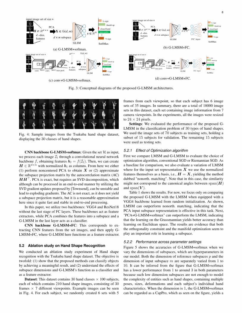
5.1 Network ArchitecturesIn the following experiments, we use network architecturescontaining the proposed methods as a layer to approach imageset recognition. The architectures are different in two separatedesign choices: (1) choice of set features, for example, raw imagesor CNN features; and (2) function of G-LMSM in the pipeline asa classifier or as a feature extractor. From these options, we canobtain the following architectures, shown on Figure 3.

G-LMSM+softmax: This is the simplest architecture, consist-ing of a G-LMSM layer and a softmax applied to the activations. In this setting, the input set is preprocessed into a subspace asfollows: Let the matrix H ∈ Rd×n contain the set images as itscolumns, where d = w ∗ h ∗ c. Then, we compute a subspacefrom the set using noncentered PCA, i.e., HH> = UΣUT . Thesubspace basis X ∈ Rd×m consists of the m leftmost columns ofU , that is, the columns with the highest corresponding eigenvalues.The subspace basis X is input in the G-LMSM layer, obtainingthe activation s ∈ RC . Each reference subspace Vj represents oneclass, and the softmax of sj corresponds to the probability of thatclass given the samples. This model corresponds to CapPro in thecase the input consists of a single vector x ∈ Rd.

G-LMSM+FC: This variation extends G-LMSM to act as afeature extractor rather than simply as a classifier, by processing sfurther through a fully-connected layer before applying softmax.The number of reference subspaces K becomes a free parameter,and the FC weights are W ∈ RK×C and b ∈ RC .

8

𝒔

MuCap

input image set of size 𝑛

conv. max-pool.conv.

𝑯 –dim.

features𝑑

ReLU ReLU

SoftMax

PCA 𝑿

ℝ𝑑 × 𝑛 𝔾(d, m)

subspace𝑑 × 𝑚

𝒔 ∈ ℝ𝑁

GLSM

input image set of size 𝑛

𝑯 ∈ ℝ𝑑 × 𝑛

–dim.features𝑑

SoftMax

open palm

L-sign

thumb up

closed hand

V-sign

PCAX ∈ 𝔾(d, m)

subspace𝑑 × 𝑚

open palm

L-sign

thumb up

closed hand

V-sign

(a) G-LMSM+softmax.

𝒔

MuCap

input image set of size 𝑛

conv. max-pool.conv.

𝑯 –dim.

features𝑑

ReLU ReLU

PCA 𝑿

subspace𝑑 × 𝑚

𝒔 ∈ ℝ𝑁

GLSM

input image set of size 𝑛

𝑯 ∈ ℝ𝑑 × 𝑛

–dim.features𝑑

SoftMax

open palm

L-sign

thumb up

closed hand

V-sign

PCA

subspace𝑑 × 𝑚𝒒

F.C. layer

SoftMax

open palm

L-sign

thumb up

closed hand

V-sign

𝒒

F.C. layer

X ∈ 𝔾(d, m)

(b) G-LMSM+FC.

𝒔

GLSM

input image set of size 𝑛

conv. max-pool.conv.

𝑯 –dim.

features𝑑

ReLU ReLU

SoftMax

PCA 𝑿

ℝ𝑑 × 𝑛 𝔾(d, m)

subspace

𝑑 × 𝑚

𝒔 ∈ ℝ𝑁

MuCap

input image set of size 𝑛

𝑯 ∈ ℝ𝑑 × 𝑛

–dim. features𝑑

SoftMax

open palm

L-sign

thumb up

closed hand

V-sign

PCAX ∈ 𝔾(d, m)

subspace𝑑 × 𝑚

open palm

L-sign

thumb up

closed hand

V-sign

(c) conv+G-LMSM+softmax.

𝒔

GLSM

input image set of size 𝑛

conv. max-pool.conv.

𝑯 –dim.

features𝑑

ReLU ReLU

PCA 𝑿

subspace𝑑 × 𝑚

𝒔 ∈ ℝ𝑁

MuCap

input image set of size 𝑛

𝑯 ∈ ℝ𝑑 × 𝑛

–dim. features𝑑

SoftMax

open palm

L-sign

thumb up

closed hand

V-sign

PCA

subspace𝑑 × 𝑚𝒒

F.C. layer

SoftMax

open palm

L-sign

thumb up

closed hand

V-sign

𝒒

F.C. layer

X ∈ 𝔾(d, m)

(d) conv+G-LMSM+FC.

Fig. 3: Conceptual diagrams of the proposed G-LMSM architectures.

Fig. 4: Sample images from the Tsukuba hand shape dataset,displaying the 30 classes of hand shapes.

CNN backbone G-LMSM+softmax: Given the setH as input,we process each image Il through a convolutional neural networkbackbone f , obtaining features hl = f(Il). Then, we can createH ∈ Rd×n with normalized hl as columns. From here we either(1) perform noncentered PCA to obtain X or (2) approximatethe subspace projection matrix by the autocorrelation matrix (AC)HH>. PCA is exact, but requires an SVD decomposition, whichalthough can be processed in an end-to-end manner by utilizing theSVD gradient updates proposed by [Townsend], can be unstable andlead to exploding gradients. The AC is not exact, as it does not yielda subspace projection matrix, but it is a reasonable approximationhere since it quite fast and stable in end-to-end processing.

In this paper, we utilize two backbones: VGG4 and ResNet18without the last stage of FC layers. These backbones act as featureextractors, while PCA combines the features into a subspace and aG-LMSM in the last layer acts as a classifier.

CNN backbone G-LMSM+FC: This corresponds to ex-tracting CNN features from the set images, and then apply G-LMSM+FC, where G-LMSM here functions as a feature extractor.

5.2 Ablation study on Hand Shape Recognition

We conducted an ablation study experiment of Hand shaperecognition with the Tsukuba hand shape dataset. The objective istwofold: (1) show that the proposed methods can classify objectsby achieving a meaningful result, and (2) understand the effects ofsubspace dimensions and G-LMSM’s function as a classifier andas a feature extractor.

Dataset: This dataset contains 30 hand classes × 100 subjects,each of which contains 210 hand shape images, consisting of 30frames × 7 different viewpoints. Example images can be seenin Fig. 4. For each subject, we randomly created 6 sets with 5

frames from each viewpoint, so that each subject has 6 imagesets of 35 images. In summary, there are a total of 18000 imagesets in this dataset, each set containing image information from 7camera viewpoints. In the experiments, all the images were resizedto 24× 24 pixels.

Settings: We evaluated the performance of the proposed G-LMSM in the classification problem of 30 types of hand shapes.We used the image sets of 70 subjects as training sets, holding asubset of 15 subjects for validation. The remaining 15 subjectswere used as testing sets.

5.2.1 Effect of Optimization algorithmFirst we compare LMSM and G-LMSM to evaluate the choice ofoptimization algorithm, conventional SGD or Riemannian SGD. Asa baseline for comparison, we also evaluate a variation of LMSMwhere for the input set representation X we use the normalizedfeatures themselves as a basis, i.e., H = X , yielding the methoddubbed "nonorth. matching". Note that in this case, the similaritymight not correspond to the canonical angles between span(H)and span(V ).

Table 1 shows the results. For now, we focus only on comparingthe proposed G-LMSM with the LMSM when equipped with aVGG4 backbone learned from random initialization. As shown,LMSM can outperform nonorth. matching, indicating that thePCA input subspace representation is effective in this task. Next,"PCA+G-LMSM+softmax" can outperform the LMSM, indicatingthat the learning on the Grassmannian yields better accuracy thanlearning on Euclidean space. The results are evidence that boththe orthogonality constraint and the manifold optimization seem toplay an important role in learning a subspace.

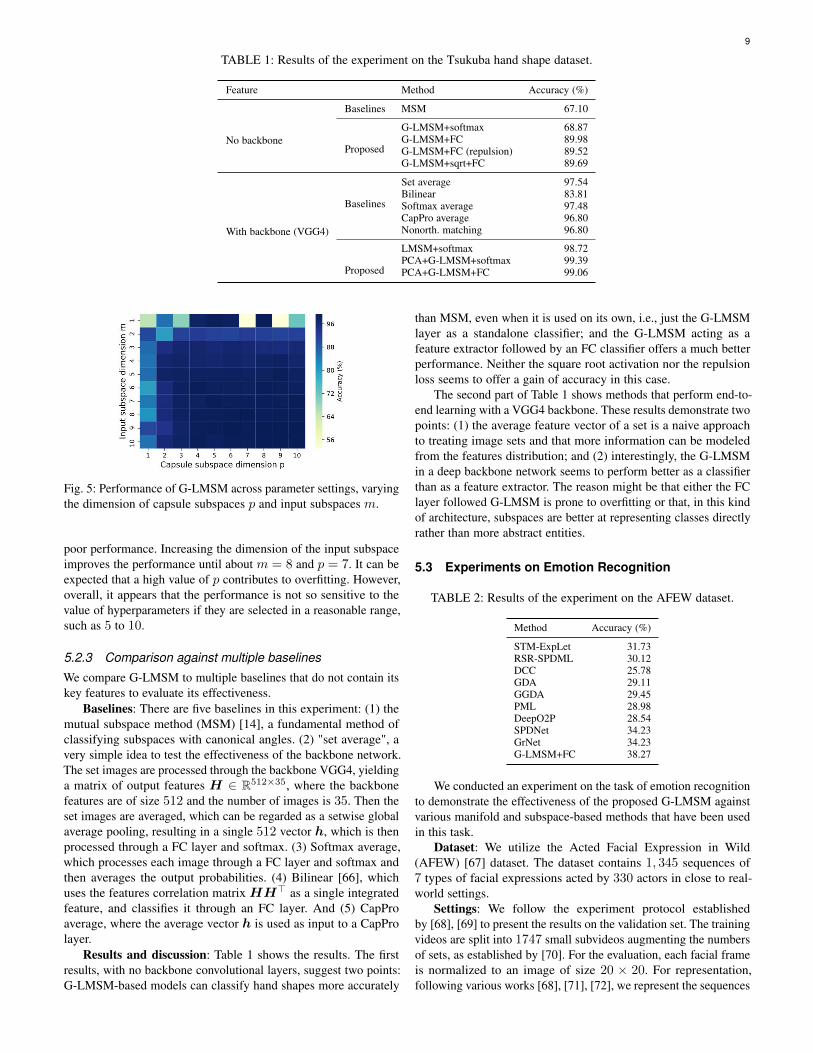
5.2.2 Performance across parameter settingsFigure 5 shows the accuracies of G-LMSM+softmax when wevary the dimensions of subspaces, which are hyperparameters inour model. Both the dimension of reference subspaces p and thedimension of input subspace m are separately varied from 1 to10. It can be inferred from the figure that G-LMSM+softmaxhas a lower performance from 1 to around 3 in both parametersbecause such low dimension subspaces are not enough to modelthe complexity of entities such as hand shapes, containing multipleposes, sizes, deformations and each subject’s individual handcharacteristics. When the dimension is 1, the G-LMSM+softmaxcan be regarded as a CapPro, which as seen on the figure, yields a

9

TABLE 1: Results of the experiment on the Tsukuba hand shape dataset.

Feature Method Accuracy (%)

No backbone

Baselines MSM 67.10

Proposed

G-LMSM+softmax 68.87G-LMSM+FC 89.98G-LMSM+FC (repulsion) 89.52G-LMSM+sqrt+FC 89.69

With backbone (VGG4)

Baselines

Set average 97.54Bilinear 83.81Softmax average 97.48CapPro average 96.80Nonorth. matching 96.80

Proposed

LMSM+softmax 98.72PCA+G-LMSM+softmax 99.39PCA+G-LMSM+FC 99.06

Fig. 5: Performance of G-LMSM across parameter settings, varyingthe dimension of capsule subspaces p and input subspaces m.

poor performance. Increasing the dimension of the input subspaceimproves the performance until about m = 8 and p = 7. It can beexpected that a high value of p contributes to overfitting. However,overall, it appears that the performance is not so sensitive to thevalue of hyperparameters if they are selected in a reasonable range,such as 5 to 10.

5.2.3 Comparison against multiple baselines

We compare G-LMSM to multiple baselines that do not contain itskey features to evaluate its effectiveness.

Baselines: There are five baselines in this experiment: (1) themutual subspace method (MSM) [14], a fundamental method ofclassifying subspaces with canonical angles. (2) "set average", avery simple idea to test the effectiveness of the backbone network.The set images are processed through the backbone VGG4, yieldinga matrix of output features H ∈ R512×35, where the backbonefeatures are of size 512 and the number of images is 35. Then theset images are averaged, which can be regarded as a setwise globalaverage pooling, resulting in a single 512 vector h, which is thenprocessed through a FC layer and softmax. (3) Softmax average,which processes each image through a FC layer and softmax andthen averages the output probabilities. (4) Bilinear [66], whichuses the features correlation matrix HH> as a single integratedfeature, and classifies it through an FC layer. And (5) CapProaverage, where the average vector h is used as input to a CapProlayer.

Results and discussion: Table 1 shows the results. The firstresults, with no backbone convolutional layers, suggest two points:G-LMSM-based models can classify hand shapes more accurately

than MSM, even when it is used on its own, i.e., just the G-LMSMlayer as a standalone classifier; and the G-LMSM acting as afeature extractor followed by an FC classifier offers a much betterperformance. Neither the square root activation nor the repulsionloss seems to offer a gain of accuracy in this case.

The second part of Table 1 shows methods that perform end-to-end learning with a VGG4 backbone. These results demonstrate twopoints: (1) the average feature vector of a set is a naive approachto treating image sets and that more information can be modeledfrom the features distribution; and (2) interestingly, the G-LMSMin a deep backbone network seems to perform better as a classifierthan as a feature extractor. The reason might be that either the FClayer followed G-LMSM is prone to overfitting or that, in this kindof architecture, subspaces are better at representing classes directlyrather than more abstract entities.

5.3 Experiments on Emotion Recognition

TABLE 2: Results of the experiment on the AFEW dataset.

Method Accuracy (%)

STM-ExpLet 31.73RSR-SPDML 30.12DCC 25.78GDA 29.11GGDA 29.45PML 28.98DeepO2P 28.54SPDNet 34.23GrNet 34.23G-LMSM+FC 38.27

We conducted an experiment on the task of emotion recognitionto demonstrate the effectiveness of the proposed G-LMSM againstvarious manifold and subspace-based methods that have been usedin this task.

Dataset: We utilize the Acted Facial Expression in Wild(AFEW) [67] dataset. The dataset contains 1, 345 sequences of7 types of facial expressions acted by 330 actors in close to real-world settings.

Settings: We follow the experiment protocol establishedby [68], [69] to present the results on the validation set. The trainingvideos are split into 1747 small subvideos augmenting the numbersof sets, as established by [70]. For the evaluation, each facial frameis normalized to an image of size 20 × 20. For representation,following various works [68], [71], [72], we represent the sequences

10

TABLE 3: Results of the experiment on the YouTube Celebrities dataset.

Type Method Accuracy (%)

Baselines

Classic

DCC 51.42 ± 4.95MMD 54.04 ± 3.69CHISD 60.42 ± 5.95PLRC 61.28 ± 6.37

Deep

DRM 66.45 ± 5.07Resnet50 vote 64.18 ± 2.20Resnet18 set average 68.24 ± 3.32Resnet18 bilinear 67.85 ± 3.35

Proposed

Features (from ResNet50) G-LMSM+FC 66.17 ± 4.19

End-to-end (backbone ResNet18)

PCA+G-LMSM+softmax 68.80 ± 3.30AC+G-LMSM+softmax 68.93 ± 3.97AC+G-LMSM+sqrt 71.09 ± 3.62AC+G-LMSM (repulsion) 70.01 ± 2.87AC+G-LMSM+temp-softmax 69.92 ± 3.79

of facial expressions with linear subspaces of dimension 10, whichexist on a Grassmann manifold G(400, 10).

Baselines: As the G-LMSM is a network layer that learnssubspaces based on iterative Riemannian optimization, we compareit against the following methods: (1) a regular CNN that can handleimage sets, namely the Deep Second-order Pooling (DeepO2P) [73].(2) Methods based on subspace without Riemannian optimization:DCC [5], Grassmann Discriminant Analysis (GDA [18] and Grass-mannian Graph-Embedding Discriminant Analysis (GGDA) [19].And (3) methods based on Riemannian optimization: ProjectionMetric Learning (PML) [74], Expressionlets on Spatio-TemporalManifold (STMExpLet) [68], Riemannian Sparse Representationcombining with Manifold Learning on the manifold of SPD matri-ces (RSR-SPDML) [75], Network on SPD manifolds (SPDNet) [69]and Grassmann net (GrNet) [72]. Especially, GrNet proposes ablock of manifold layers for subspace data. GrNet-1 denotes thearchitecture with 1 block and GrNet-2 with 2 blocks.

Results and discussion: The results can be seen in Table 2.The proposed method achieved quite competitive results comparedto the manifold-based methods, by mapping the subspace into avector and then uses simple Euclidean operations such as fully-connected layers and cross-entropy loss, in contrast to severalmethods that use complex approaches requiring multiple matrixdecompositions. First, G-LMSM+softmax outperforms popularmethods such as GDA and GGDA, which have a similar purposeof mapping Grassmann manifold data into a vector representation.The reason is perhaps that G-LMSM learns both the representationand discrimination in an end-to-end manner, while GDA uses akernel function to represent subspaces and learns the discriminantindependently. Methods such as SPDNet and GrNet are composedof many complex layers involving SVD, QR decompositions, andGram–Schmidt orthogonalization and its derivatives are utilized aswell. They increase in complexity as the number of layers increasesby repeating these operations, which are not easily scalable touse in GPUs. On the other hand, the proposed method providescompetitive results with fewer layers and no decompositions,making it naturally parallelizable and scalable.

5.4 Experiment on Face Identification

We conducted an experiment of face identification with theYouTube Celebrities (YTC) dataset. Dataset: The YTC dataset [76]contains 1910 videos of 47 identities. Similarly to [77], as an imageset, we used a set of face images extracted from a video by theIncremental Learning Tracker [78]. All the extracted face imageswere scaled to 30 × 30 pixels and converted to grayscale.

Settings: Three videos per each person were randomly selectedas training data, and six videos per each person were randomlyselected as test data. We repeated the above procedure five timesand measured the average accuracy.

Baselines: (1) Classic image set-based methods: DiscriminativeCanonical Correlations (DCC) [5], manifold-manifold distance(MMD) [79], Convex Hull-based Image Set Distance (CHISD) [43],Pairwise linear regression classification (PLRC) [30]. (2) Deeplearning methods: deep reconstruction model (DRM) [80]; Resnetvote [81] is a baseline consisting of a Resnet50 [81] fine-tuned tothis dataset with the cross-entropy loss in a single image setting.For the fine-tuning, we added two fully connected (FC) layersafter the last global average pooling layer in the network. The firstFC layer outputs a 1024 dimension vector through the ReLU [82]function, and the second layer outputs a 47 (the number of classes)dimension vector through the softmax function. Hyperparametersof the optimizer were used as suggested by the original paper. Forclassification, each image of a set is classified independently and amajority voting strategy of all predictions is used to select a singleclass prediction for the whole set. The model called Resnet18set average is the same as used in the hand shape experiment.The Resnet18 bilinear model uses the correlation matrix of thebackbone features of the image set, generating a 512× 512 matrix.The vectorized matrix is processed through an FC layer and softmaxfor classification.

Results and discussion: Table 3 shows the results. G-LMSMoutperforms not only the classical manifold methods, but alsovarious deep methods. Although G-LMSM uses the same backboneas some methods, it still can achieve better results. In the case ofResnet50 vote and the G-LMSM+FC, the key difference is thatvoting is a simple heuristic approach to image set recognition, asthe model is not aware of the set as a whole. This leads to unstableand diverging predictions on a set’s class, as it does not take intoaccount the underlying set distribution. The voting method is notdifferentiable by nature, so it is not trivial to extend this idea to anend-to-end approach. Then, set average seems again to be a naiveapproach to treating image sets and that more information can bemodeled from the features distribution. The bilinear model could intheory capture the underlying set information from the correlations,but the high dimensionality of the correlation matrix makes italmost impossible to learn a FC classifier without overfitting.

These results confirm the advantage of G-LMSM over thesemethods using the same backbone: mutual subspaces providea low-dimensional, differentiable approach to modeling the setdistribution, ultimately leading to a straightforward integration of

11

the deep convolutional networks and the problem of image sets.Furthermore, the AC+G-LMSM+softmax seems to yield the

same result as PCA+G-LMSM+softmax, evidence that it is a goodapproximation for processing the input data. Then, the proposedvariations of G-LMSM, namely, repulsion loss, the square rootactivation and the temperature softmax (temp-softmax) appear toprovide an advantage over the base G-LMSM. “

6 CONCLUSION

In this paper, we addressed the problem of image set recognition.We proposed two subspace-based methods, named learning mutualsubspace method (LMSM) and Grassmannian learning mutualsubspace method (G-LMSM), that can recognize image sets withDNN as feature extractors in an end-to-end fashion. The proposedmethods generalize the classic average learning subspace method(ALSM), in that LMSM and G-LMSM can handle an image set asinput and perform subspace matching. The key idea of G-LMSM isto learn the subspaces with Riemannian stochastic gradient descenton the Grassmann manifold, ensuring each parameter is always anorthogonal basis of a subspace.

Extensive experiments on hand shape recognition, face iden-tification, and facial emotion recognition showed that LMSMand G-LMSM have a high discriminant ability in image setrecognition. It can be used easily as a standalone method orwithin larger DNN frameworks. The experiments also reveal thatRiemannian optimization is effective in learning G-LMSM withinneural networks.

REFERENCES

[1] A. Shashua, “On Photometric Issues in 3D Visual Recognitionfrom a Single 2D Image,” International Journal of ComputerVision, vol. 21, no. 1, pp. 99–122, Jan. 1997. [Online]. Available:https://doi.org/10.1023/A:1007975506780

[2] P. N. Belhumeur and D. J. Kriegman, “What Is the Set of Images ofan Object Under All Possible Illumination Conditions?” InternationalJournal of Computer Vision, vol. 28, no. 3, pp. 245–260, Jul. 1998.[Online]. Available: https://doi.org/10.1023/A:1008005721484

[3] K.-C. Lee, J. Ho, and D. J. Kriegman, “Acquiring linear subspaces forface recognition under variable lighting,” IEEE Transactions on patternanalysis and machine intelligence, vol. 27, no. 5, pp. 684–698, 2005.

[4] R. Basri and D. W. Jacobs, “Lambertian reflectance and linear subspaces,”IEEE transactions on pattern analysis and machine intelligence, vol. 25,no. 2, pp. 218–233, 2003.

[5] T.-K. Kim, J. Kittler, and R. Cipolla, “Discriminative learning andrecognition of image set classes using canonical correlations,” IEEETransactions on Pattern Analysis and Machine Intelligence, vol. 29, no. 6,pp. 1005–1018, 2007.

[6] N. Sogi, R. Zhu, J.-H. Xue, and K. Fukui, “Constrained mutual convexcone method for image set based recognition,” Pattern Recognition, vol.121, p. 108190, 2022.

[7] L. S. Souza, B. B. Gatto, J.-H. Xue, and K. Fukui, “Enhanced grass-mann discriminant analysis with randomized time warping for motionrecognition,” Pattern Recognition, vol. 97, p. 107028, 2020.

[8] S. Watanabe and N. Pakvasa, “Subspace method of pattern recognition,”in Proc. 1st. IJCPR, 1973, pp. 25–32.

[9] T. Iijima, H. Genchi, and K.-i. Mori, “A theory of character recognitionby pattern matching method,” in Learning systems and intelligent robots.Springer, 1974, pp. 437–450.

[10] E. Oja, Subspace methods of pattern recognition. Research Studies Press,1983, vol. 6.

[11] A. S. Georghiades, P. N. Belhumeur, and D. J. Kriegman, “From fewto many: Illumination cone models for face recognition under variablelighting and pose,” IEEE transactions on pattern analysis and machineintelligence, vol. 23, no. 6, pp. 643–660, 2001.

[12] H. Hotelling, “Relations between two sets of variates,” in Breakthroughsin statistics. Springer, 1992, pp. 162–190.

[13] S. N. Afriat, “Orthogonal and oblique projectors and the characteristics ofpairs of vector spaces,” in Mathematical Proceedings of the CambridgePhilosophical Society, vol. 53, no. 4. Cambridge University Press, 1957,pp. 800–816.

[14] K. Fukui and A. Maki, “Difference subspace and its generalization forsubspace-based methods,” Pattern Analysis and Machine Intelligence,IEEE Transactions on, vol. 37, no. 11, pp. 2164–2177, 2015.

[15] O. Yamaguchi and K. Fukui, “Smartface–a robust face recognition systemunder varying facial pose and expression,” 2003.

[16] K. Fukui and O. Yamaguchi, “The kernel orthogonal mutual subspacemethod and its application to 3d object recognition,” in Asian Conferenceon Computer Vision. Springer, 2007, pp. 467–476.

[17] H. Sakano and N. Mukawa, “Kernel mutual subspace method forrobust facial image recognition,” in KES’2000. Fourth InternationalConference on Knowledge-Based Intelligent Engineering Systems andAllied Technologies. Proceedings (Cat. No. 00TH8516), vol. 1. IEEE,2000, pp. 245–248.

[18] J. Hamm and D. D. Lee, “Grassmann discriminant analysis: a unifyingview on subspace-based learning,” in Proceedings of the 25th internationalconference on Machine learning. ACM, 2008, pp. 376–383.

[19] ——, “Extended grassmann kernels for subspace-based learning,” inAdvances in neural information processing systems, 2009, pp. 601–608.

[20] T. Kohonen, G. Németh, K.-J. Bry, M. Jalanko, and H. Riittinen, “Spectralclassification of phonemes by learning subspaces,” in ICASSP’79. IEEEInternational Conference on Acoustics, Speech, and Signal Processing,vol. 4. IEEE, 1979, pp. 97–100.

[21] E. Oja and M. Kuusela, “The ALSM algorithm — an improved subspacemethod of classification,” Pattern Recognition, vol. 16, no. 4, pp. 421–427,1983.

[22] P.-A. Absil, R. Mahony, and R. Sepulchre, “Riemannian geometry ofgrassmann manifolds with a view on algorithmic computation,” ActaApplicandae Mathematica, vol. 80, no. 2, pp. 199–220, 2004.

[23] A. A. Borisenko and Y. A. Nikolaevskii, “Grassmann manifolds andthe grassmann image of submanifolds,” Russian mathematical surveys,vol. 46, no. 2, pp. 45–94, 1991.

[24] K. Fujii, “Introduction to grassmann manifolds and quantum computation,”Journal of Applied Mathematics, vol. 2, no. 8, pp. 371–405, 2002.

[25] O.-E. Ganea and G. Bécigneul, “Riemannian adaptive optimizationmethods,” in 7th International Conference on Learning Representations(ICLR 2019), 2018.

[26] S. Bonnabel, “Stochastic gradient descent on riemannian manifolds,” IEEETransactions on Automatic Control, vol. 58, no. 9, pp. 2217–2229, 2013.

[27] L. Wang, H. Cheng, and Z. Liu, “A set-to-set nearest neighborapproach for robust and efficient face recognition with imagesets,” Journal of Visual Communication and Image Representation,vol. 53, pp. 13–19, May 2018. [Online]. Available: https://www.sciencedirect.com/science/article/pii/S1047320318300300

[28] W. Wang, R. Wang, S. Shan, and X. Chen, “Discriminative CovarianceOriented Representation Learning for Face Recognition with Image Sets,”in 2017 IEEE Conference on Computer Vision and Pattern Recognition(CVPR). Honolulu, HI: IEEE, Jul. 2017, pp. 5749–5758. [Online].Available: http://ieeexplore.ieee.org/document/8100092/

[29] J. Lu, G. Wang, W. Deng, P. Moulin, and J. Zhou, “Multi-manifolddeep metric learning for image set classification,” in Proceedings of theIEEE conference on computer vision and pattern recognition, 2015, pp.1137–1145.

[30] Q. Feng, Y. Zhou, and R. Lan, “Pairwise Linear Regression Classificationfor Image Set Retrieval,” in 2016 IEEE Conference on Computer Visionand Pattern Recognition (CVPR), Jun. 2016, pp. 4865–4872, iSSN: 1063-6919.

[31] I. Naseem, R. Togneri, and M. Bennamoun, “Linear Regression forFace Recognition,” IEEE Transactions on Pattern Analysis and MachineIntelligence, vol. 32, no. 11, pp. 2106–2112, Nov. 2010, conference Name:IEEE Transactions on Pattern Analysis and Machine Intelligence.

[32] J. Stallkamp, H. K. Ekenel, and R. Stiefelhagen, “Video-based FaceRecognition on Real-World Data,” in 2007 IEEE 11th InternationalConference on Computer Vision, Oct. 2007, pp. 1–8, iSSN: 2380-7504.

[33] S. Zhou and R. Chellappa, “Probabilistic Human Recognition from Video,”in Computer Vision — ECCV 2002, ser. Lecture Notes in ComputerScience, A. Heyden, G. Sparr, M. Nielsen, and P. Johansen, Eds. Berlin,Heidelberg: Springer, 2002, pp. 681–697.

[34] J. R. Uijlings, K. E. Van De Sande, T. Gevers, and A. W. Smeulders,“Selective search for object recognition,” International journal of computervision, vol. 104, no. 2, pp. 154–171, 2013.

[35] X. Li, K. Fukui, and N. Zheng, “Boosting constrained mutual subspacemethod for robust image-set based object recognition,” in Twenty-FirstInternational Joint Conference on Artificial Intelligence, 2009.

12

[36] K. Jarrett, K. Kavukcuoglu, M. Ranzato, and Y. LeCun, “What is thebest multi-stage architecture for object recognition?” in 2009 IEEE 12thinternational conference on computer vision. IEEE, 2009, pp. 2146–2153.

[37] Z.-Q. Zhao, S.-T. Xu, D. Liu, W.-D. Tian, and Z.-D. Jiang, “A review ofimage set classification,” Neurocomputing, vol. 335, pp. 251–260, 2019.

[38] O. Arandjelovic, G. Shakhnarovich, J. Fisher, R. Cipolla, and T. Darrell,“Face recognition with image sets using manifold density divergence,” in2005 IEEE Computer Society Conference on Computer Vision and PatternRecognition (CVPR’05), vol. 1. IEEE, 2005, pp. 581–588.

[39] K.-i. Maeda, O. Yamaguchi, and K. Fukui, “Towards 3-dimensionalpattern recognition,” in Joint IAPR International Workshops on StatisticalTechniques in Pattern Recognition (SPR) and Structural and SyntacticPattern Recognition (SSPR). Springer, 2004, pp. 1061–1068.

[40] T.-K. Kim and R. Cipolla, “Canonical correlation analysis of video volumetensors for action categorization and detection,” IEEE Transactions onPattern Analysis and Machine Intelligence, vol. 31, no. 8, pp. 1415–1428,2009.

[41] R. Wang, S. Shan, X. Chen, Q. Dai, and W. Gao, “Manifold–manifolddistance and its application to face recognition with image sets,” IEEETransactions on Image Processing, vol. 21, no. 10, pp. 4466–4479, 2012.

[42] R. Wang and X. Chen, “Manifold discriminant analysis,” in 2009 IEEEConference on Computer Vision and Pattern Recognition. IEEE, 2009,pp. 429–436.

[43] H. Cevikalp and B. Triggs, “Face recognition based on image sets,” in2010 IEEE Computer Society Conference on Computer Vision and PatternRecognition. IEEE, 2010, pp. 2567–2573.

[44] Y. Hu, A. S. Mian, and R. Owens, “Face recognition using sparseapproximated nearest points between image sets,” IEEE transactions onpattern analysis and machine intelligence, vol. 34, no. 10, pp. 1992–2004,2012.

[45] ——, “Sparse approximated nearest points for image set classification,”in CVPR 2011. IEEE, 2011, pp. 121–128.

[46] M. Harandi, C. Sanderson, C. Shen, and B. C. Lovell, “Dictionary learningand sparse coding on grassmann manifolds: An extrinsic solution,” inProceedings of the IEEE international conference on computer vision,2013, pp. 3120–3127.

[47] M. Liao and X. Gu, “Face recognition based on dictionary learning andsubspace learning,” Digital Signal Processing, vol. 90, pp. 110–124, 2019.

[48] J. Hamm, “Subspace-based learning with grassmann kernels,” 2008.[49] M. T. Harandi, C. Sanderson, S. Shirazi, and B. C. Lovell, “Graph em-

bedding discriminant analysis on Grassmannian manifolds for improvedimage set matching,” in Computer Vision and Pattern Recognition, IEEEConference on. IEEE, 2011, pp. 2705–2712.

[50] L. Souza, H. Hino, and K. Fukui, “3d object recognition with enhancedgrassmann discriminant analysis,” in ACCV 2016 Workshop (HIS 2016),2016.

[51] P. Zhu, H. Cheng, Q. Hu, Q. Wang, and C. Zhang, “Towards Generalizedand Efficient Metric Learning on Riemannian Manifold,” Proceedingsof the Twenty-Seventh International Joint Conference on ArtificialIntelligence, pp. 3235–3241, 2018.

[52] N. Sogi, L. S. Souza, B. B. Gatto, and K. Fukui, “Metric learning witha-based scalar product for image-set recognition,” in Proceedings ofthe IEEE/CVF Conference on Computer Vision and Pattern RecognitionWorkshops, 2020, pp. 850–851.

[53] L. Luo, J. Xu, C. Deng, and H. Huang, “Robust Metric Learning onGrassmann Manifolds with Generalization Guarantees,” Proceedings ofthe AAAI Conference on Artificial Intelligence, vol. 33, pp. 4480–4487,2019.

[54] L. Zhang, M. Edraki, and G.-J. Qi, “Cappronet: Deep feature learning viaorthogonal projections onto capsule subspaces,” in Advances in neuralinformation processing systems, 2018.

[55] G. E. Hinton, A. Krizhevsky, and S. D. Wang, “Transforming auto-encoders,” in International conference on artificial neural networks.Springer, 2011, pp. 44–51.

[56] S. Sabour, N. Frosst, and G. E. Hinton, “Dynamic routing betweencapsules,” arXiv preprint arXiv:1710.09829, 2017.

[57] S. Watanabe, “Evaluation and selection of variables in pattern recognition,”Computer and Information Science II, pp. 91–122, 1967.

[58] T. Iijima, “A theoretical study of pattern recognition by matching method,”in Proc. of First USA-Japan Computer Conf., 1972, 1972, pp. 42–48.

[59] A. Edelman, T. A. Arias, and S. T. Smith, “The geometry of algorithmswith orthogonality constraints,” SIAM journal on Matrix Analysis andApplications, vol. 20, no. 2, pp. 303–353, 1998.

[60] G. Bécigneul and O.-E. Ganea, “Riemannian adaptive optimizationmethods,” arXiv preprint arXiv:1810.00760, 2018. [Online]. Available:https://openreview.net/forum?id=r1eiqi09K7

[61] X. Yang, Y. Chen, and H. Liang, “Square root based activation function inneural networks,” in 2018 International Conference on Audio, Languageand Image Processing (ICALIP). IEEE, 2018, pp. 84–89.

[62] C. Guo, G. Pleiss, Y. Sun, and K. Q. Weinberger, “On calibrationof modern neural networks,” in International Conference on MachineLearning. PMLR, 2017, pp. 1321–1330.

[63] G. Hinton, O. Vinyals, and J. Dean, “Distilling the knowledge in a neuralnetwork,” arXiv preprint arXiv:1503.02531, 2015.

[64] S. Liang, Y. Li, and R. Srikant, “Enhancing the reliability of out-of-distribution image detection in neural networks,” arXiv preprintarXiv:1706.02690, 2017.

[65] A. Agarwala, J. Pennington, Y. Dauphin, and S. Schoenholz, “Temperaturecheck: theory and practice for training models with softmax-cross-entropylosses,” arXiv preprint arXiv:2010.07344, 2020.

[66] Y. Gao, O. Beijbom, N. Zhang, and T. Darrell, “Compact bilinear pooling,”in Proceedings of the IEEE conference on computer vision and patternrecognition, 2016, pp. 317–326.

[67] A. Dhall, R. Goecke, J. Joshi, K. Sikka, and T. Gedeon, “Emotionrecognition in the wild challenge 2014: Baseline, data and protocol,”in Proceedings of the 16th international conference on multimodalinteraction. ACM, 2014, pp. 461–466.

[68] M. Liu, S. Shan, R. Wang, and X. Chen, “Learning expressionlets onspatio-temporal manifold for dynamic facial expression recognition,” inProceedings of the IEEE Conference on Computer Vision and PatternRecognition, 2014, pp. 1749–1756.

[69] Z. Huang and L. Van Gool, “A riemannian network for spd matrix learning,”in Thirty-First AAAI Conference on Artificial Intelligence, 2017.

[70] Z. Huang, J. Wu, and L. V. Gool, “Building Deep Networks on GrassmannManifolds,” arXiv, 2016.

[71] M. Liu, R. Wang, Z. Huang, S. Shan, and X. Chen, “Partial leastsquares regression on grassmannian manifold for emotion recognition,” inProceedings of the 15th ACM on International conference on multimodalinteraction. ACM, 2013, pp. 525–530.

[72] Z. Huang, J. Wu, and L. Van Gool, “Building deep networks on grassmannmanifolds,” in Thirty-Second AAAI Conference on Artificial Intelligence,2018.

[73] C. Ionescu, O. Vantzos, and C. Sminchisescu, “Training deep networkswith structured layers by matrix backpropagation,” arXiv preprintarXiv:1509.07838, 2015.

[74] Z. Huang, R. Wang, S. Shan, and X. Chen, “Projection metric learningon grassmann manifold with application to video based face recognition,”in Proceedings of the IEEE conference on computer vision and patternrecognition, 2015, pp. 140–149.

[75] M. T. Harandi, M. Salzmann, and R. Hartley, “From manifold to manifold:Geometry-aware dimensionality reduction for spd matrices,” in Europeanconference on computer vision. Springer, 2014, pp. 17–32.

[76] M. Kim, S. Kumar, V. Pavlovic, and H. Rowley, “Face tracking andrecognition with visual constraints in real-world videos,” in ComputerVision and Pattern Recognition. IEEE, 2008, pp. 1–8.

[77] S. A. A. Shah, U. Nadeem, M. Bennamoun, F. A. Sohel, and R. Togneri,“Efficient image set classification using linear regression based imagereconstruction.” in Computer Vision and Pattern Recognition Workshops,2017, pp. 601–610.

[78] D. A. Ross, J. Lim, R.-S. Lin, and M.-H. Yang, “Incremental learning forrobust visual tracking,” International Journal of Computer Vision, vol. 77,no. 1-3, pp. 125–141, 2008.

[79] R. Wang, S. Shan, X. Chen, and W. Gao, “Manifold-manifold distancewith application to face recognition based on image set,” in 2008 IEEEConference on Computer Vision and Pattern Recognition. IEEE, 2008,pp. 1–8.

[80] S. A. Shah, U. Nadeem, M. Bennamoun, F. Sohel, and R. Togneri,“Efficient image set classification using linear regression based imagereconstruction,” in Proceedings of the IEEE Conference on ComputerVision and Pattern Recognition Workshops, 2017, pp. 99–108.

[81] K. He, X. Zhang, S. Ren, and J. Sun, “Deep residual learning for imagerecognition,” in The IEEE Conference on Computer Vision and PatternRecognition, 2016.

[82] V. Nair and G. E. Hinton, “Rectified linear units improve restrictedboltzmann machines,” in Proceedings of the 27th International Conferenceon Machine Learning, 2010, pp. 807–814.