Model-Shared Subspace Boosting for Multi-labelClassification

Rong YanIBM TJ Watson Research

19 Skyline Dr.Hawthorne, NY, 10523

yanr@us.ibm.com

Jelena TesicIBM TJ Watson Research

19 Skyline Dr.Hawthorne, NY, 10523

jtesic@us.ibm.com

John R. SmithIBM TJ Watson Research

19 Skyline Dr.Hawthorne, NY, 10523

jsmith@us.ibm.com

ABSTRACTTypical approaches to the multi-label classification prob-lem require learning an independent classifier for every la-bel from all the examples and features. This can become acomputational bottleneck for sizeable datasets with a largelabel space. In this paper, we propose an efficient and ef-fective multi-label learning algorithm called model-sharedsubspace boosting (MSSBoost) as an attempt to reduce theinformation redundancy in the learning process. This algo-rithm automatically finds, shares and combines a numberof base models across multiple labels, where each model islearned from random feature subspace and bootstrap datasamples. The decision functions for each label are jointly es-timated and thus a small number of shared subspace modelscan support the entire label space. Our experimental resultson both synthetic data and real multimedia collections havedemonstrated that the proposed algorithm can achieve bet-ter classification performance than the non-ensemble base-line classifiers with a significant speedup in the learning andprediction processes. It can also use a smaller number ofbase models to achieve the same classification performanceas its non-model-shared counterpart.

Categories and Subject DescriptorsH.1.0 [Information System]: Models and Principles

General TermsAlgorithms, Performance, Theory

KeywordsMulti-label classification, random subspace methods, boost-ing, model sharing

1. INTRODUCTIONMulti-label classification is a concept in learning systems

that refers to the simultaneous categorization of a given in-

Permission to make digital or hard copies of all or part of this work forpersonal or classroom use is granted without fee provided that copies arenot made or distributed for profit or commercial advantage and that copiesbear this notice and the full citation on the first page. To copy otherwise, torepublish, to post on servers or to redistribute to lists, requires prior specificpermission and/or a fee.KDD’07, August 12–15, 2007, San Jose, California, USA.Copyright 2007 ACM 978-1-59593-609-7/07/0008 ...$5.00.

put example into a set of multiple labels. The need formulti-label classification in large-scale systems is increasingin diverse applications such as music categorization, imageand video annotation, text categorization and medical ap-plications. Detecting multiple semantic labels from imagesbased on their low-level visual features [2, 15, 14] and auto-matically classifying text documents into a number of topicsbased on their textual context [25, 18] are some of the typi-cal multi-label applications. In reality, multimedia and textdata collections can contain hundred thousands to millionsof data items, and these items can be associated with thou-sands of different labels. Most existing algorithms do notscale well to such a high computational demand, becausethey need to learn an independent classifier for every possi-ble label using all the data samples and the entire featurespace. Thus it is a great challenge and opportunity for us todesign more advanced multi-label learning algorithms thatcan learn and predict multiple labels in an accurate andefficient way.

To speed up multi-label classification without performancedegradation, one approach is to exploit the information re-dundancy in the learning space. To this end, researchershave proposed several ensemble learning algorithms basedon random feature selection and data bootstrapping. Therandom subspace method (RSM) [12] takes advantage ofboth feature space bootstrapping and model aggregation,and combines multiple base models learned on a randomlyselected subset of the feature space. RSM considerably re-duces the size of the feature space in each base model, andthe model computation is more efficient than a classifier di-rectly built on the entire feature space. Combining bagging(bootstrap aggregation) and RSM, Breiman has developeda more general algorithm called random forest [4]. Randomforest aims to aggregate an ensemble of unpruned classi-fication/regression trees using both bootstrapped trainingexamples and random feature selection in the tree induc-tion process. Random forest can be learned more efficientlythan the baseline method, and it has empirically demon-strated superiority compared to a single tree classifier. Forthe multi-label scenario, above algorithms need to learn anindependent classifier for every label or assume that the un-derlying base models can produce multi-label predictions.

However, they ignore an important fact that different la-bels are not independent of each other, or orthogonal to oneanother. On the contrary, multiple labels are usually inter-related and connected by their semantic interpretations, andhence exhibit certain co-occurrence patterns in the data col-lections. For example, in an image collection, the label “car”

Research Track Paper

834

Label 1Label 2Label 3Others

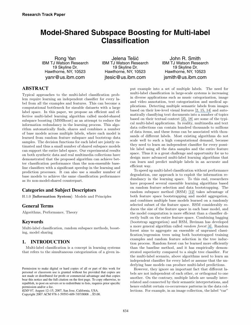
Figure 1: Redundancy in the decision space demon-strated using a 2-D synthetic dataset with 3 labels.The dashed circles indicate the true decision bound-ary for each label.

almost always co-occurs with the label “road”, while theconcept “office” is not likely to appear with “road”. Inter-related multi-labels exhibit the redundancy of informationin the label space. This observation inspires us to furtherimprove the classification efficiency by exploiting the labelspace redundancy. To achieve this goal in an ensemble learn-ing algorithm, we can allow the underlying base models tobe shared across multiple labels and thus the decisions ofbase models can be re-used in several places at the sametime. To illustrate, Figure 1 shows a 2-D synthetic datasetwith 3 labels, where its characteristics are explained in Sec-tion 6.1. Let us assume that each base model is learnedfrom a depth-1 decision tree that can only produce an axis-parallel decision boundary. In this case, if these models arenot allowed to be shared, we need at least 12 base modelsto construct accurate classifiers for all three labels, becauseeach label requires at least 4 models for capturing its bound-aries. However, as we can observe, the decision boundariesof all three labels are closely related to each other. As itresults, only 5 base models are needed to construct classi-fiers of a similar quality, if these models can be shared acrossmultiple decision functions.

In this paper, we propose a boosting-type learning algo-rithm called model-shared subspace boosting (MSSBoost).It merges ensemble learning, random subspace sampling,and models sharing techniques to automatically find, shareand combine a number of random subspace models acrossmultiple labels. MSSBoost is able to reduce the informa-tion redundancy in the label space by jointly optimizing theloss functions over all possible labels. Meanwhile, since itsbase models are built on a small number of bootstrap datasamples and a randomly selected feature subspace, the pro-posed algorithm can scale to sizeable datasets with a largenumber of labels. Our experiments show that MSSBoostcan outperform the non-ensemble baseline classifiers with asignificant speedup on the learning and prediction process.It can also use a smaller number of base models to achievethe same classification performance as its non-model-sharedcounterpart. As a by-product, the proposed algorithm canautomatically discover the underlying context between mul-tiple labels, and this offers us more insights to analyze thedata collections.

Our following discussions are organized as follows. Sec-tion 2 presents the basic notations and terminologies usedin this paper. Section 3 illustrates the random space bag-

ging methods in detail. Section 4 describes the proposedMSSBoost algorithm and analyzes its learning propertiesas well as its computational complexity. Section 5 reviewsthe related efforts and compares them with our approaches.Section 6 presents the experimental results on multiple datacollections and Section 7 concludes our discussions.

2. PRELIMINARIESIn this section, we present the formal notations and termi-

nologies that we use in our study. Let X be the domain of allpossible features, and the number of features for X is M . LetY be a finite set of labels of size L, L = |Y|. Without loss ofgenerality, we assume the labels are {1, ..., L}. In the multi-label classification setting, each data point x ∈ X can be as-signed multiple labels from Y. For instance, for an image an-notation problem where “building”, “sky” and “water” arethe possible labels, we can associate an image with the labelsof both “building” and “sky”. Let yl ∈ {−1, +1} indicate ifthe data example x belongs to the lth label, l ∈ [1, L]. There-fore, we can represent a labeled example as (x,y), wherey = {yl}l=1..L. Given a set of training data {(xi,yi)}i=1..N ,the goal of the multi-label learning algorithms is to producea decision function of the form F : X × Y → R. Here weuse a simpler representation by assuming each label l has itsown decision function Fl : X → R, and the correspondingprediction yl is determined by sign(Fl(x)).

Ensemble learning approaches such bagging [3] and boost-ing [8] aim to improve the classification performance by com-bining the outputs from a family of base models H, a.k.a.weak learners. Each base model h ∈ H is a binary classifierthat produces a real-valued predictions 1 h : X → R, and weassume |h(·)| ≤ 1. The base models can be generated fromdifferent types of algorithms such as decision tree and sup-port vector machines. Some classification algorithms alsoattempt to optimize a loss function C(y, f), i.e. AdaBoostuses the exponential loss C(y, f) = exp(yf(·)), and Logit-Boost uses the logistic loss C(y, f) = log(1 + exp(yf(·))).Given the base models available, the learning algorithmscan find a linear combination of base models to construct acomposite decision function, F (x) =

∑t αtht(x), where αt

is the combination weight.

3. RANDOM SUBSPACE BAGGINGBagging, boosting and the random subspace method are

among the most popular ensemble learning approaches. Bag-ging approach was proposed by Breiman [3], and it incorpo-rates the approaches of bootstrapping and classifier aggrega-tion. Multiple sets of training examples can be generated byrandom sampling the original training set with replacement.The decision functions based on multiple samples can beaggregated by majority voting or averaging. Previous the-oretical and empirical results have shown that bagging canreduce the variance of the prediction outputs and thus sig-nificantly improve the performance of unstable classifiers [3].However, a simple bagging approach can under-perform inthe imbalanced set scenarios, because as multi-label classi-fication problem often faces imbalance distribution in thedataset, the bootstrap examples may only contain few oreven none of the minority labeled data. As shown by recent

1This setting is more general than most previous work [18] which

assumes the base models have to produce multi-label outputs h :X × Y → R.

Research Track Paper

835

Algorithm 1 The round-robin random subspace bagging(RSBag) algorithm for multi-label classification.

Input: training data {xi,yi}i=1...N , xi ∈ RM , number of

total base models T , number of labels L, data sampling ratiord(≤ 1), feature sampling ratio rf (≤ 1).

1. For t = 1 to T,

(a) Choose a label l = μ(t), where μ(·) is the remain-der over L;

(b) Take a bootstrap sample Xt+ from the positive

data {xi} for l (i.e., yil = 1), |Xt+| = Nrd/2;

(c) Take a bootstrap sample Xt− from the negative

data {xi} for l (i.e., yil = −1), |Xt−| = Nrd/2;

(d) Take a random sample F t from the feature indices{1, ..., M}, |F t| = Mrf ;

(e) Learn a base model ht(x) using Xt+, Xt

− and F t.

(f) Fl(x)← Fl(x) + ht(x).

2. Output the classifier yl = sign[Fl(x)].

studies [22, 7], artificially making the class prior equal bydown sampling is usually more effective and efficient thansimple bagging. This technique is called “asymmetric bag-ging” or “balanced bagging”.

The random subspace method (RSM) [12] is another ex-ample of ensemble learning approach that takes advantagesof bootstrapping and aggregating classifiers. However, in-stead of bootstrapping the training samples, RSM modifiesthe data examples from the other dimension by randomly se-lecting a subset of the features to learn the base models. Byreducing the size of the feature space, RSM can usually becomputed more efficiently than the baseline. The learningperformance of RSM can benefit from operating on a smallnumber of features, especially when the number of trainingexamples are insufficient. In this case, more stable classifierscan be built with a relatively larger amount of training datawith respect to the feature space.

The connections between bagging and RSM has inspiredthe development of a more general algorithm called randomforest [4], which aggregate an ensemble of unpruned clas-sification/regression trees using both bootstrapped trainingexamples and random feature selection in the tree inductionprocess. Random forest has empirically demonstrated to beable to outperform a single tree classifier such as CART andC4.5. It also yields a generalization error comparable withAdaBoost. However, ensemble learning approaches were notlimited to tree classifiers. The extended idea of bagging wasapplied in a video retrieval task [16], and the random forestidea was used in an image retrieval task [22]. In general, weterm the algorithmic combination of bagging and randomsubspace selection as “random subspace bagging” (RSBag)classifiers (a.k.a., Asymmetric Bagging and Random Sub-space classifiers in previous work [22]), and define it as,

Definition 1. A random subspace bagging classifier is acomposite classifier combining a collection of base models{h(x, Θt)}Tt=1 where {Θt} are independent identically dis-tributed random vectors. Each classifier generates a predic-tion output based on training data and Θt. 2

2Θt can have different semantics: in bagging Θt can be a boot-

To apply the random subspace bagging algorithms for themulti-label classification problem, we present a round-robinrandom subspace bagging approach in Algorithm 1. Thisalgorithm first selects a label to work with in a round robinfashion. Then we learn a base model based on Nrd bal-anced bootstrap samples from the positive and the negativedata, together with Mrf random samples from the featureindices, where rd is called the data sampling ratio and rf iscalled the feature sampling ratio. Both sampling ratios aredetermined by the input parameters and typically they areless than 1. At the end we aggregate all the base models forthe same label into a composite classifier. This algorithm issimilar to a balanced version of random forests [22, 7] withthe random vectors Θt as the indices of Xt

+, Xt− and F t.

The only difference is that it can use any binary classifierto construct the base models without being limited to thedecision trees. To shed lights on why the random subspacebagging works, we present an upper bound for its generaliza-tion error. The importance of the interaction between twoingredients, the model strength s and the model correlationρ, for minimizing the upper bound on the classification erroris shown in the following theorem:

Theorem 1. For each label l in the random subspace bag-ging algorithms described in Algorithm 1, an upper bound forthe generalization error is given by,

E∗(Fl) ≤ ρ(1− s2l )/s2

l ,

where sl is the strength of base models for the label l, i.e.,

sl = 2Ex,ylPΘ(h(x, Θ) = yl)− 1,

and ρ is the correlation between any two base models, i.e.,

ρ = EΘ,Θ′[ρx(h(x,Θ), h(x, Θ′))

].

Proof: Immediately follow the proof of Theorem 2.3 in [4]by viewing multi-label classification as a set of binary clas-sification problems on each label l. �

Therefore, classification accuracy can be improved by min-imizing the model correlation ρ while maintaining the modelstrength s. Randomly sampling the training examples andfeature subspace is useful to diversify the base models, andmeanwhile reduce the model size. As long as the quality ofeach bootstrap models is not significantly deteriorated, ran-dom subspace bagging is able to generate a classifier withsmaller model size, while produce a comparable performancewith the single classifier learned from the entire data space.This claim is confirmed by the experiments in Section 6.

4. MODEL-SHARED SUBSPACE BOOSTINGThe base models learned from bootstrap samples and fea-

ture subspace provide a foundation for developing scalableensemble learning algorithms for multi-label classification.However, because the base models are learned independentlyon each label, they may contain redundant decision informa-tion that can be shared across a number of labels. By ex-ploiting this kind of information redundancy, we can furtherreduce the size of ensemble classifiers and keep the classi-fication performance intact. To automatically discover thebase models that can be shared among labels, we switch the

strapped sample from the integers from 1 to the number of data N ,and in RSM Θt can be a number of independent random integersbetween 1 to the number of features M .

Research Track Paper

836

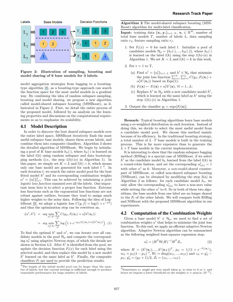
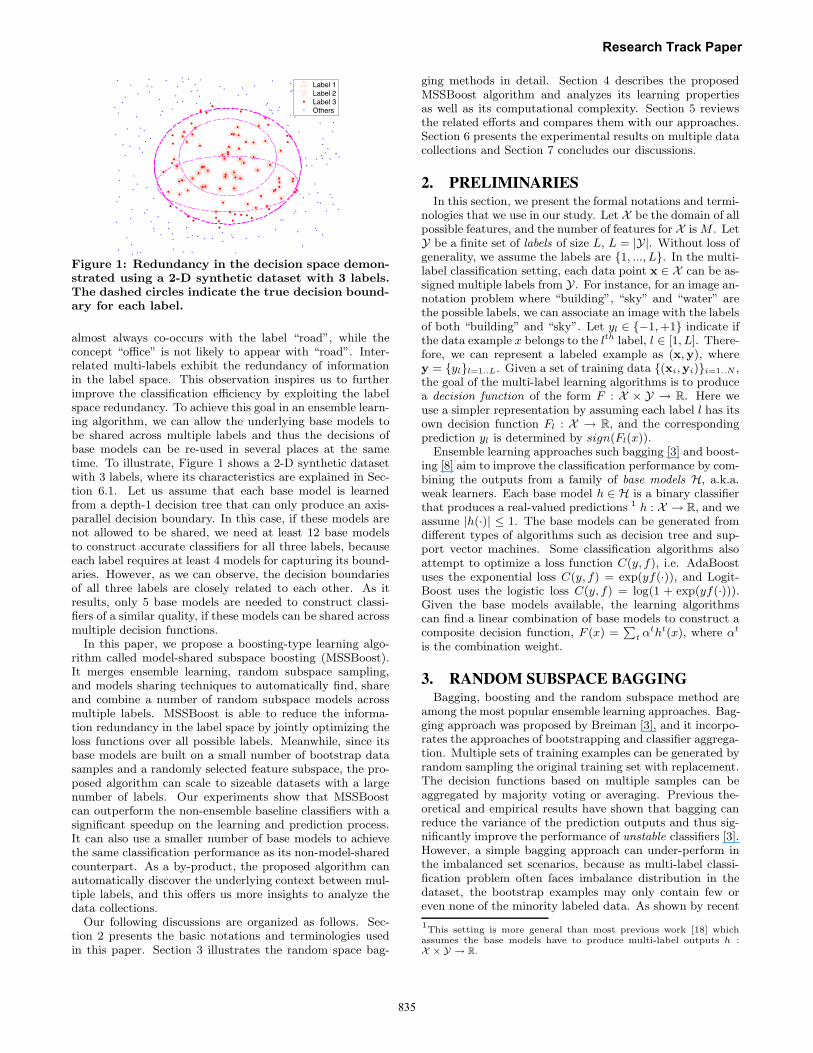
Figure 2: Illustration of sampling, boosting andmodel sharing of 6 base models for 3 labels.

model aggregation strategies from bagging to a boosting-type algorithm [8], as a boosting-type approach can searchthe function space for the most useful models in a gradientway. By combining the idea of random subspace sampling,boosting and model sharing, we propose a new algorithmcalled model-shared subspace boosting (MSSBoost), as il-lustrated in Figure 2. First, we detail the entire process ofthe proposed model, followed by an analysis on the learn-ing properties and discussions on the computational require-ments so as to emphasize its scalability.

4.1 Model DescriptionIn order to discover the best shared subspace models over

the entire label space, MSSBoost iteratively finds the mostuseful subspace base models, shares them across labels, andcombine them into composite classifiers. Algorithm 2 showsthe detailed algorithm of MSSBoost. We begin by initializ-ing a pool of K base models hk(·), where hk(·) is learned onthe label l(k) using random subspace and data bootstrap-ping methods (i.e., the step 1(b)-(e) in Algorithm 1). Inthis paper, we simply set K = L and l(k) = k, which meansonly one base model are generated for each label l 3. Ineach iteration t, we search the entire model pool for the bestfitted model ht and its corresponding combination weightsαt = {αt

l}Ll=1. This can be achieved by minimizing a jointlogistic loss function summed over all the labels. One impor-tant issue here is to select a proper loss function. Extremeloss functions such as the exponential loss functions are notrobust against outliers, because they tend to assign muchhigher weights to the noisy data. Following the idea of Log-itBoost [9], we adopt a logistic loss C(y, f) = log(1 + e−yf )and thus the optimization step can be rewritten as,

{αt, ht} = arg minαt,ht

∑il

C(yil, Fl(xi) + αtlh

t(xi))

= arg minαt

l,ht

∑il

log(1 + e−yil(Fl(xi)+αt

lht(xi)))

. (1)

To find the optimal ht and αt, we can iterate over all can-didate models in the pool Hp and compute the correspond-ing αt

l using adaptive Newton steps, of which the details areshown in Section 4.2. After ht is identified from the pool, weupdate the decision function Fl(x) for each label using theselected model, and then replace this model by a new modelht learned on the same label as ht. Finally, the compositeclassifiers Fl are used to provide the prediction results.3The length of the initial model pool can be larger than the num-

ber of labels, but the current settings is sufficient enough to producereasonable performance for large number of labels.

Algorithm 2 The model-shared subspace boosting (MSS-Boost) algorithm for multi-label classification.

Input: training data {xi, yi}i=1..N , xi ∈ RM , number of

total base models T , number of labels L, data samplingratio rd, feature sampling ratio rf .

1. Set Fl(x) = 0 for each label l. Initialize a pool ofcandidate models Hp = {h1(·), ..., hK(·)}, where hk(·)is learned on the label l(k) using the step 1(b)-(e) inAlgorithm 1. We set K = L and l(k) = k in this work.

2. For t = 1 to T,

(a) Find αt = {αtl}l=1..L and ht ∈ Hp that minimize

the joint loss function∑N

i=1

∑Ll=1 C(yil, Fl(xi) +

αtlh

t(xi)) based on Eqn(1);

(b) Fl(x)← Fl(x) + αtlh

t(x), ∀l = 1...L;

(c) Replace ht in Hp with a new candidate model ht,which is learned on the same label as ht using thestep 1(b)-(e) in Algorithm 1.

3. Output the classifier yl = sign[Fl(x)].

Remark: Typical boosting algorithms learn base modelsusing a re-weighted distribution in each iteration. Instead ofdoing this, we decide to select the most useful model froma candidate model pool. We choose this method mainlybecause of its efficiency. In the traditional boosting strategy,a total number of L · T base models is built in the trainingprocess. This is far more expensive than to generate theL + T base models in the current implementation.

It is interesting to show that the random subspace baggingmethod (RSBag) is a special case of MSSBoost, if we selectht as the candidate model hk learned from the label l(k) ina round-robin fashion, and set the corresponding αt

l(k) = 1

with other αt as 0. Moreover, a non-model-shared counter-part of MSSBoost, or called non-shared subspace boosting(NSBoost), can be obtained by modifying the step 3(a) inAlgorithm 2 as follows: for each candidate model hk, weonly allow the corresponding αt

l(k) to have a non-zero value

while setting the other αt to 0. So in both of these two algo-rithms, the base models from one label are no longer sharedto the Fl of the other labels. We will compare both RSBagand NSBoost with the proposed MSSBoost algorithm in ourexperiments.

4.2 Computation of the Combination WeightsGiven a base model ht ∈ Hp, we need to find a set of

combination weights αt that helps to minimize the joint lossfunction. To this end, we apply an efficient adaptive Newtonalgorithm. Adaptive Newton algorithm can be summarizedas the following weighted least-squares regression step:

αtl = (HT WlH)−1HT Zl, (2)

where H = (ht(x1), ..., ht(xN ))T , pil = 1/(1 + e−Fl(xi)),

wil = pil(1− pil)4, Wl = diag(wl1, ..., wlN ) and zil = y′

il −pil, y′

il = (yil + 1)/2, Zl = (zl1, ..., zlN).

4Sometimes wi might get very small when pi is close to 0 or 1, and

hence we impose a lower threshold on the weights w = max(w, 10−6).

Research Track Paper

837

Proposition 1. Eqn(2) is a one-step adaptive Newtonupdate for the joint logistic loss function.

Proof: Let us consider the update Fl(x)+αtlh

t(x) and thejoint loss function with respect to αt,

C(αt) =∑

i

∑l

C(yil, Fl(xi) + αtlh

t(xi))

We can compute the first derivative and second derivativeat αt

l = 0,∀l,∂C(αt)

∂αtl

|αtl=0=

∑i

yilht(xi)

1 + eyilFl(xi)= HT Zl,

∂C2(αt)

∂αt2l

|αtl=0=

∑i

[ht(xi)]2

2 + eyilFl(xi) + e−yilFl(xi)= HT WlH.

Therefore the Newton update can be written as,

αlt ←

[∂C2(αt)

∂αt2l

]−1∂C(αt)

∂αtl

= (HT WlH)−1HT Zl.

�For each model ht in the candidate model pool, we can

compute its corresponding combination weights αt. ThenEqn(1) is applied to find the best pair of {αt, ht} that canbest minimize the joint loss function. Theoretically, ratherthan only running one-step update, we can compute mul-tiple consecutive steps of Newton updates in the step 2(a)of Algorithm 2 in order to get a better estimate for αt

l periteration. However, since the boosting update also aims tooptimize the same criterion in the outer loop, increasing thenumber of consecutive Newton updates inside will bring lit-tle advantage on the final prediction results. Therefore weonly run one-step Newton update to compute each αt

l . Thisstrategy is also adopted in [9].

4.3 Analysis of Learning PropertiesIn this section, we analyze two learning properties for the

proposed algorithm. First, we derive an upper bound forthe cumulative training error over all the labels:

Theorem 2. Let Fil = Fl(xi). The following upper boundholds for the cumulative training error,∑

i

∑l

I(sign(Fil) �= yil) ≤∑

i

∑l

C(yil, Fil),

where I(x) = 1 if x is true and otherwise I(x) = 0.

Proof: Based on the inequalities log(1+e−x) > 0 and whenx ≤ 0, log(1 + e−x) ≥ 1, we can show that

∑i

∑l

I(sign(Fil �= yil) ≤∑

yilFil �=0

log(1 + e−yilFil

)

≤∑

i

∑l

log(1 + e−yilFil

),

where the right hand side is exactly∑

i

∑l C(yil, Fil) based

on its definition. �Theorem 2 suggests that it is reasonable for the MSS-

Boost algorithm to directly optimize the joint logistic lossfunction, which serves as an upper bound for the training er-ror over all the labels. Therefore minimizing this joint lossfunction can guarantee to produce a low training error inthe learning process. Next, we show the proposed algorithm

also satisfy the boosting property [17], i.e., if the hypothesisspace of base models satisfy the “weak learnability” (i.e., theweighted margin of base models is at least λ > 0 in each it-eration), the loss function will go towards 0 with sufficientlylarge training samples, and thus the generalization error willgo to 0 with an increasing margin [9]. The satisfaction ofthe boosting property can be proved as follows,

Theorem 3. Suppose the base models hk in the candidatepool satisfy the weak learnability for the label l(k), i.e.,∑

i wil(k)yl(k)hk(xi)∑i wil(k)

≥ λ > 0,∀k = 1...K (3)

where wil is the sampling distribution ∂C(yil,Fil)∂Fil

= 1

1+eyi1Fi1

for the ith data example. Then for any value S0, we can

show that after at most T = 2N4L4

λ2S20

rounds we can obtain a

joint loss C(·) no more than S0L.

Proof Sketch: Let Ctl be the total loss for the label l in

iteration t, i.e., Ctl =

∑i C(yil, Fil), and the joint loss is

Ct =∑

l Ctl . If the condition Ct ≥ S0L satisfies, there must

be one Ctl ≥ S0. Without loss of generality, let us assume

Ct1 ≥ S0. In the following we will show the improvement

in the joint loss function is at leastλ2S2

02N3L3 if the candidate

model h1 (learned on the label 1) is selected from the modelpool. For the sake of simplicity, we ignore the iteration indext in the rest of the discussion unless stated otherwise.

Because the joint loss function is minimized in each itera-tion, C1 must be less than the initial joint loss NL and thuslog(1+ e−yi1Fi1) ≤ NL, ∀i. By combining this fact with thefollowing inequality,

− log γ ≥ 1− γ ≥ 1− γ0

log γ0log γ, if 0 ≤ γ0 ≤ γ ≤ 1,

where γ0 is a constant, we can have

log(1 + e−yi1Fi1) ≥ 1

1 + eyi1Fi1≥ β0 log(1 + e−yi1Fi1),∀i (4)

where β0 = (1 − 2−NL)/NL. Since N and L is large ingeneral, we can simplify β0 = 1/NL.

Using the inequalities in (3) and (4), we can derive anlower bound for the negative gradient of C1 w.r.t. α1,

−∑

i

∂C(yi1, Fi1 + α1hi1)

∂α1|α1=0=

∑i

1

1 + eyi1Fi1· yi1hi1

≥ λ∑

i

1

1 + eyi1Fi1≥ λβ0

∑i

log(1 + e−yi1Fi1) ≥ λS0

NL. (5)

Next, we bound the second derivative of the change in theloss function under the assumption that |hi1| ≤ 1,

∑i

∂2C(yi1, Fi1 + α1hi1)

∂α21

|α1=0≤∑

i

h2i1

1 + eyi1Fi1≤ NL. (6)

If we combine the two bounds together and take a stepsize α1 = λS0

N2L2 , the reduction of the loss function C1 is at

leastλ2S2

02N3L3 according to Taylor’s theorem. Since the loss

function of the other labels will at least be unaffected, the

joint loss function C will also at least be reduced byλ2S2

02N3L3 .

In this case, if a different candidate model hk′ is selectedin MSSBoost, its joint loss reduction must be more thanusing h1 based on our model selection criterion. Now since

Research Track Paper

838

the initial joint loss is NL and thus within this number of

iterations, T = 2N4L4

λ2S20

, we must get a non-positive loss if we

still have a joint loss large than S0L. This obviously gives acontradiction and thus the boosting property is proved. �

4.4 Computational ComplexityThe computational complexity of MSSBoost mainly comes

from (a) the generation of base models from bootstrappeddata/feature spaces, and (b) minimization of the joint lossfunction using adaptive Newton steps. Since the second steponly involves the operations of matrix computations and ascalar inverse, its effect on the computational complexity ofthe overall system is not influential as the calculations aremuch faster than a generation of base models in first step.

As noted in Section 4.1, our current implementation needsto generate L+T base models in total, where each model islearned with Nrd examples and Mrf features. Thus the to-tal time is (L+T ) · tl(Nrd, Mrf ), where tl(n, m) is the basemodel learning time with n examples and m features. Sim-ilarly, the total prediction time is T · tp(Nrd, Mrf ), wheretp(n, m) is the base model prediction time. The form of tl

and tp is determined by the choice of the underlying basemodels. For example, the learning time of decision trees istl(n, m) = O(mn log n) (Chapter 9 in [11]) and the predic-tion time is tp(n, m) = O(mn) if we assume the base modelsize is proportional to the number of data and features.Most current support vector machine(SVM) implementa-tions such as [13] have a learning time of tl(n, m) = O(mn2)and a prediction time of tp(n, m) = O(mn) if the numberof support vectors is proportional to the number of train-ing data. Compared with a baseline classifier that learnsa model from N examples and M features for each label,MSSBoost can achieve a speedup of T+L

Lrdrf in learning

and TL

rdrf in prediction with decision trees. Similarly, with

SVMs, MSSBoost can achieve a speedup of T+LL

r2drf and

TL

rdrf in learning and prediction respectively. This can re-sult in a significant speedup in general. For instance, if weset rd = 0.1, rf = 0.1 and T = 3L, the learning and predic-tion time of MSSBoost with SVMs can be reduced around250 times and 33 times over the baseline.

5. RELATED WORK AND DISCUSSIONSEnsemble learning approaches such as boosting and bag-

ging [8, 3, 18] have been demonstrated to be effective in im-proving the classification accuracy of weak learned models.By combining the idea of ensemble learning with randomsubspace methods, random forest [4] shows the possibilityof developing efficient and effective classifiers using a setof tree models. The similar idea has also been applied tothe task of image retrieval with SVMs as the base mod-els [22]. Along another line, Caruana et al. [6] proposedan ensemble selection approach for choosing the most usefulmodels from a large model library via a forward stepwiseselection method. However, since most ensemble learningapproaches are developed on binary classification, their ex-tensions to multi-label classification either need to maintainindependent binary classifiers for each label, or require theunderlying models to be able to generate multi-label out-puts, which prevent them from capturing the common repre-sentations across labels in the ensemble aggregation level. Inthis sense, the AdaBoost.OC algorithm [19] is a more closelyrelated to our work, which merges AdaBoost with the Error-

Correcting Output Codes (ECOC) to handle the multi-classlearning problem with a pool of binary classifiers. It onlyneeds to keep track of one set of data distributions for mul-tiple classes at the same time. However, because multi-classlearning problems assume each data point can only associateone single class, their algorithm is not directly applicable tothe multi-label problem.

In the machine learning community, the idea of sharingthe common information among multiple labels have beeninvestigated by the methods called “multi-task learning”,which has also been known as “transfer learning” and “learn-ing to learn”. These methods handle the multi-label classi-fication problem by treating each label as a single task andgeneralizing the correlations among multiple tasks. Fromanother viewpoint, they can also be thought as learning acommon feature representation across all the tasks. Manymethods have been proposed for multi-task learning, suchas neural networks [5], regularization learning methods [1],hierarchical Bayesian models [26] and so on. For exam-ple, Zhang et al. [26] proposed a latent variable model formulti-task learning which assumes that tasks are sparse lin-ear combination of basic classifiers. Ghamrawi et al. [10]proposed a multilabel conditional random field classifica-tion model that directly parameterize label co-occurrences inmulti-label classification. The listed approaches are usuallymore computationally expensive than the baseline single-task learning algorithms because they often use the single-task learners in an iterative process and require a complexinference effort to estimate the task parameters. This clearlycontrasts with the MSSBoost algorithm which can consider-ably improve the learning efficiency in multi-label scenarios.In addition, MSSBoost can be build on any base modelswithout being limited to a specific type.

The problem of exploring and leveraging the connectionsacross labels have also been seen in many other researchareas. One such example is the domain of image annota-tion and object recognition which aims to detect a numberof scenes and objects in the given images. For instance,Snoek et al. [21] proposed an semantic value chain architec-ture including a multi-label learning layer called context link.Yan et al. [24] studied various multi-label relational learn-ing approaches via a unified probabilistic graphical modelrepresentation. However, these methods need to constructan additional computational intensive layer on top of thebase models, and they do not provide any mechanisms toreduce the redundancy among labels other than utilizing themulti-label relations. Torralba et al. [23] developed a jointboosting algorithm that finds the common image featuresshared across multiple labels. But this method are specif-ically built above the level of image features rather thanthe general base models in our methods. In addition, itslearning process is computationally demanding, as it needsto search either 2L− 1 sharing patterns or L(L + 1)/2 in itssimplified version.

6. EXPERIMENTSWe demonstrate the effectiveness and efficiency of the pro-

posed MSSBoost algorithm on several multi-label data col-lections, including a synthetic dataset and two real-worldmultimedia collections. The statistics of the data collectionsare summarized in Table 1.

Research Track Paper

839

12

3

4

5

67

8

Label 1Label 2Label 3

Label 1Label 2Label 3

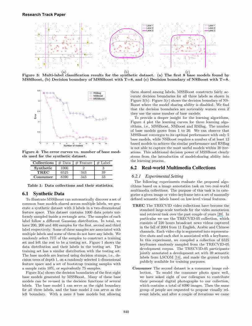
(a) (b) (c)Figure 3: Multi-label classification results for the synthetic dataset. (a) The first 8 base models found byMSSBoost, (b) Decision boundary of MSSBoost with T=8, and (c) Decision boundary of NSBoost with T=8.

0 2 4 6 8 10 12 14 16 18 200

0.05

0.1

0.15

0.2

0.25

Err

or

Number of models

RSBagNSBoostMSSBoost

Figure 4: The error curves vs. number of base mod-els used for the synthetic dataset.

Collections # Data # Feature # Label

Synthetic 1000 2 3TREC 6525 343 39

Consumer 8390 343 33

Table 1: Data collections and their statistics.

6.1 Synthetic DataTo illustrate MSSBoost can automatically discover a set of

common base models shared across multiple labels, we gen-erate a synthetic dataset with 3 labels in a two-dimensionalfeature space. This dataset contains 1000 data points uni-formly sampled inside a rectangle area. The samples of eachlabel follow a different Gaussian distribution. In total, wehave 200, 200 and 400 samples for the first, second and thirdlabel respectively. Some of these samples are associated withmultiple labels and some of them do not have any labels. Werandomly select 75% of the samples to construct a trainingset and left the rest to be a testing set. Figure 1 shows thedata distribution and their labels in the testing set. Thetraining set has a similar distribution with the testing set.The base models are learned using decision stumps, i.e., de-cision trees of depth 1, on a randomly selected 1-dimensionalfeature space and a set of bootstrap training samples witha sample ratio 10%, or equivalently 75 samples.

Figure 3(a) shows the decision boundaries of the first eightbase models generated by MSSBoost. Many of these basemodels can be re-used in the decision functions of severallabels. The base model 1 can serve as the right boundaryfor all three labels, and the base model 2 can serve as theleft boundary. With a mere 8 base models but allowing

them shared among labels, MSSBoost constructs fairly ac-curate decision boundaries for all three labels as shown inFigure 3(b). Figure 3(c) shows the decision boundary of NS-Boost where the model sharing ability is disabled. We findthat the decision boundaries are noticeably worsen even ifthey use the same number of base models.

To provide a deeper insight for the learning algorithms,Figure 4 plot the learning curves for three learning algo-rithms, i.e., MSSBoost, NSBoost and RSBag. The numberof base models grows from 1 to 20. We can observe thatMSSBoost converges to its optimal performance with only 5base models, while NSBoost requires a number of at least 12based models to achieve the similar performance and RSBagis not able to capture the most useful models within 20 iter-ations. This additional decision power of MSSBoost clearlystems from the introduction of model-sharing ability intothe learning process.

6.2 Real-world Multimedia Collections

6.2.1 Experimental SettingThe following experiments evaluate the proposed algo-

rithms based on a image annotation task on two real-worldmultimedia collections. The purpose of this task is to cate-gorize a given image or video keyframe into a set of manuallydefined semantic labels based on low-level visual features.

TREC The TRECVID video collections have become thestandard large-scale testbeds for the video annotationand retrieval task over the past couple of years [20]. Inparticular we use the TRECVID-05 collection, whichconsists of 220 hours broadcast news videos capturedin the fall of 2004 from 11 English, Arabic and Chinesechannels. Each video clip is segmented into representa-tive shots and each shot is associated with a keyframe.In this experiment, we compiled a collection of 6525keyframes randomly sampled from the TRECVID-05development corpus. The TRECVID-05 participantsjointly annotated a development set with 39 semanticlabels from LSCOM [14], and made the ground truthpublicly available for training purposes.

Consumer The second dataset is a consumer image col-lection. To model the consumer photo space well,we have asked eight of our colleagues to contributetheir personal digital photographs to our collection,which contains a total of 8390 images. Then the samegroup of people are requested to propose visually rel-evant labels, and after a couple of iterations we came

Research Track Paper

840

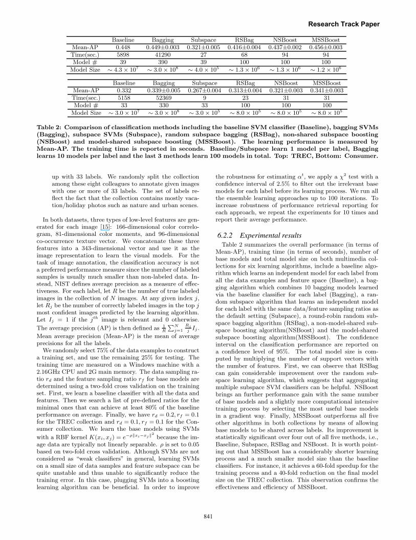
Baseline Bagging Subspace RSBag NSBoost MSSBoostMean-AP 0.448 0.449±0.003 0.321±0.005 0.416±0.004 0.437±0.002 0.456±0.003Time(sec.) 5898 41290 27 68 94 94Model # 39 390 39 100 100 100

Model Size ∼ 4.3× 107 ∼ 3.0 × 108 ∼ 4.0× 105 ∼ 1.3× 106 ∼ 1.3× 106 ∼ 1.2 × 106

Baseline Bagging Subspace RSBag NSBoost MSSBoostMean-AP 0.332 0.339±0.005 0.267±0.004 0.313±0.004 0.321±0.003 0.341±0.003Time(sec.) 5158 52369 9 23 31 31Model # 33 330 33 100 100 100

Model Size ∼ 3.0× 107 ∼ 3.0× 108 ∼ 3.0 × 105 ∼ 8.0× 105 ∼ 8.0× 105 ∼ 8.0× 105

Table 2: Comparison of classification methods including the baseline SVM classifier (Baseline), bagging SVMs(Bagging), subspace SVMs (Subspace), random subspace bagging (RSBag), non-shared subspace boosting(NSBoost) and model-shared subspace boosting (MSSBoost). The learning performance is measured byMean-AP. The training time is reported in seconds. Baseline/Subspace learn 1 model per label, Bagginglearns 10 models per label and the last 3 methods learn 100 models in total. Top: TREC, Bottom: Consumer.

up with 33 labels. We randomly split the collectionamong these eight colleagues to annotate given imageswith one or more of 33 labels. The set of labels re-flect the fact that the collection contains mostly vaca-tion/holiday photos such as nature and urban scenes.

In both datasets, three types of low-level features are gen-erated for each image [15]: 166-dimensional color correlo-gram, 81-dimensional color moments, and 96-dimensionalco-occurrence texture vector. We concatenate these threefeatures into a 343-dimensional vector and use it as theimage representation to learn the visual models. For thetask of image annotation, the classification accuracy is nota preferred performance measure since the number of labeledsamples is usually much smaller than non-labeled data. In-stead, NIST defines average precision as a measure of effec-tiveness. For each label, let R be the number of true labeledimages in the collection of N images. At any given index j,let Rj be the number of correctly labeled images in the top jmost confident images predicted by the learning algorithm.Let Ij = 1 if the jth image is relevant and 0 otherwise.

The average precision (AP) is then defined as 1R

∑Nj=1

Rj

jIj .

Mean average precision (Mean-AP) is the mean of averageprecisions for all the labels.

We randomly select 75% of the data examples to constructa training set, and use the remaining 25% for testing. Thetraining time are measured on a Windows machine with a2.16GHz CPU and 2G main memory. The data sampling ra-tio rd and the feature sampling ratio rf for base models aredetermined using a two-fold cross validation on the trainingset. First, we learn a baseline classifier with all the data andfeatures. Then we search a list of pre-defined ratios for theminimal ones that can achieve at least 80% of the baselineperformance on average. Finally, we have rd = 0.2, rf = 0.1for the TREC collection and rd = 0.1, rf = 0.1 for the Con-sumer collection. We learn the base models using SVMs

with a RBF kernel K(xi, xj) = e−ρ‖xi−xj‖2because the im-

age data are typically not linearly separable. ρ is set to 0.05based on two-fold cross validation. Although SVMs are notconsidered as “weak classifiers” in general, learning SVMson a small size of data samples and feature subspace can bequite unstable and thus unable to significantly reduce thetraining error. In this case, plugging SVMs into a boostinglearning algorithm can be beneficial. In order to improve

the robustness for estimating αt, we apply a χ2 test with aconfidence interval of 2.5% to filter out the irrelevant basemodels for each label before its learning process. We run allthe ensemble learning approaches up to 100 iterations. Toincrease robustness of performance retrieval reporting foreach approach, we repeat the experiments for 10 times andreport their average performance.

6.2.2 Experimental resultsTable 2 summarizes the overall performance (in terms of

Mean-AP), training time (in terms of seconds), number ofbase models and total model size on both multimedia col-lections for six learning algorithms, include a baseline algo-rithm which learns an independent model for each label fromall the data examples and feature space (Baseline), a bag-ging algorithm which combines 10 bagging models learnedvia the baseline classifier for each label (Bagging), a ran-dom subspace algorithm that learns an independent modelfor each label with the same data/feature sampling ratios asthe default setting (Subspace), a round-robin random sub-space bagging algorithm (RSBag), a non-model-shared sub-space boosting algorithm(NSBoost) and the model-sharedsubspace boosting algorithm(MSSBoost). The confidenceinterval on the classification performance are reported ona confidence level of 95%. The total model size is com-puted by multiplying the number of support vectors withthe number of features. First, we can observe that RSBagcan gain considerable improvement over the random sub-space learning algorithm, which suggests that aggregatingmultiple subspace SVM classifiers can be helpful. NSBoostbrings an further performance gain with the same numberof base models and a slightly more computational intensivetraining process by selecting the most useful base modelsin a gradient way. Finally, MSSBoost outperforms all fiveother algorithms in both collections by means of allowingbase models to be shared across labels. Its improvement isstatistically significant over four out of all five methods, i.e.,Baseline, Subspace, RSBag and NSBoost. It is worth point-ing out that MSSBoost has a considerably shorter learningprocess and a much smaller model size than the baselineclassifiers. For instance, it achieves a 60-fold speedup for thetraining process and a 40-fold reduction on the final modelsize on the TREC collection. This observation confirms theeffectiveness and efficiency of MSSBoost.

Research Track Paper

841

10 20 30 40 50 60 70 80 90 1000.1

0.15

0.2

0.25

0.3

0.35

0.4

0.45

0.5

Number of Models

Mea

n A

vera

ge P

reci

sion

BaselineRSBagNSBoostMSSBoost

10 20 30 40 50 60 70 80 90 1000.05

0.1

0.15

0.2

0.25

0.3

0.35

Number of Models

Mea

n A

vera

ge P

reci

sion

BaselineRSBagNSBoostMSSBoost

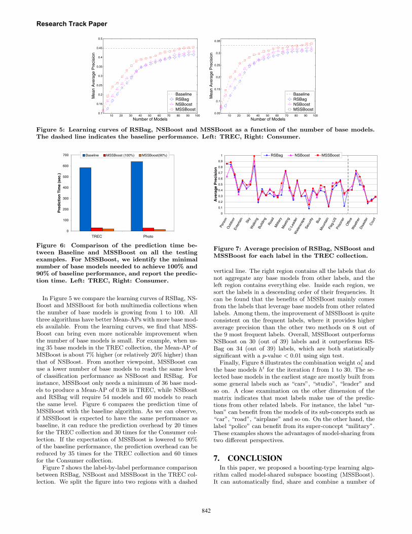
Figure 5: Learning curves of RSBag, NSBoost and MSSBoost as a function of the number of base models.The dashed line indicates the baseline performance. Left: TREC, Right: Consumer.

0

100

200

300

400

500

600

700

TREC Photo

Pre

dic

tio

n T

ime

(sec

.)

Baseline MSSBoost (100%) MSSBoost(90%)

Figure 6: Comparison of the prediction time be-tween Baseline and MSSBoost on all the testingexamples. For MSSBoost, we identify the minimalnumber of base models needed to achieve 100% and90% of baseline performance, and report the predic-tion time. Left: TREC, Right: Consumer.

In Figure 5 we compare the learning curves of RSBag, NS-Boost and MSSBoost for both multimedia collections whenthe number of base models is growing from 1 to 100. Allthree algorithms have better Mean-APs with more base mod-els available. From the learning curves, we find that MSS-Boost can bring even more noticeable improvement whenthe number of base models is small. For example, when us-ing 35 base models in the TREC collection, the Mean-AP ofMSBoost is about 7% higher (or relatively 20% higher) thanthat of NSBoost. From another viewpoint, MSSBoost canuse a lower number of base models to reach the same levelof classification performance as NSBoost and RSBag. Forinstance, MSSBoost only needs a minimum of 36 base mod-els to produce a Mean-AP of 0.38 in TREC, while NSBoostand RSBag will require 54 models and 60 models to reachthe same level. Figure 6 compares the prediction time ofMSSBoost with the baseline algorithm. As we can observe,if MSSBoost is expected to have the same performance asbaseline, it can reduce the prediction overhead by 20 timesfor the TREC collection and 30 times for the Consumer col-lection. If the expectation of MSSBoost is lowered to 90%of the baseline performance, the prediction overhead can bereduced by 35 times for the TREC collection and 60 timesfor the Consumer collection.

Figure 7 shows the label-by-label performance comparisonbetween RSBag, NSBoost and MSSBoost in the TREC col-lection. We split the figure into two regions with a dashed

0

0.1

0.2

0.3

0.4

0.5

0.6

0.7

0.8

0.9

1

Pers

onO

utdo

orEn

terta

in

Sky

Wal

king

Build

ing

Roa

dM

ilitar

yM

eetin

gC

-Lea

der

Wat

ersc

ape

Secu

rity

Bus

Mou

ntai

nFl

ag-U

SPr

ison

erO

ffice

Wea

ther

Dis

aste

rC

ourt

Ave

rag

e P

reci

sio

n

RSBag NSBoost MSSBoost

Figure 7: Average precision of RSBag, NSBoost andMSSBoost for each label in the TREC collection.

vertical line. The right region contains all the labels that donot aggregate any base models from other labels, and theleft region contains everything else. Inside each region, wesort the labels in a descending order of their frequencies. Itcan be found that the benefits of MSSBoost mainly comesfrom the labels that leverage base models from other relatedlabels. Among them, the improvement of MSSBoost is quiteconsistent on the frequent labels, where it provides higheraverage precision than the other two methods on 8 out ofthe 9 most frequent labels. Overall, MSSBoost outperformsNSBoost on 30 (out of 39) labels and it outperforms RS-Bag on 34 (out of 39) labels, which are both statisticallysignificant with a p-value < 0.01 using sign test.

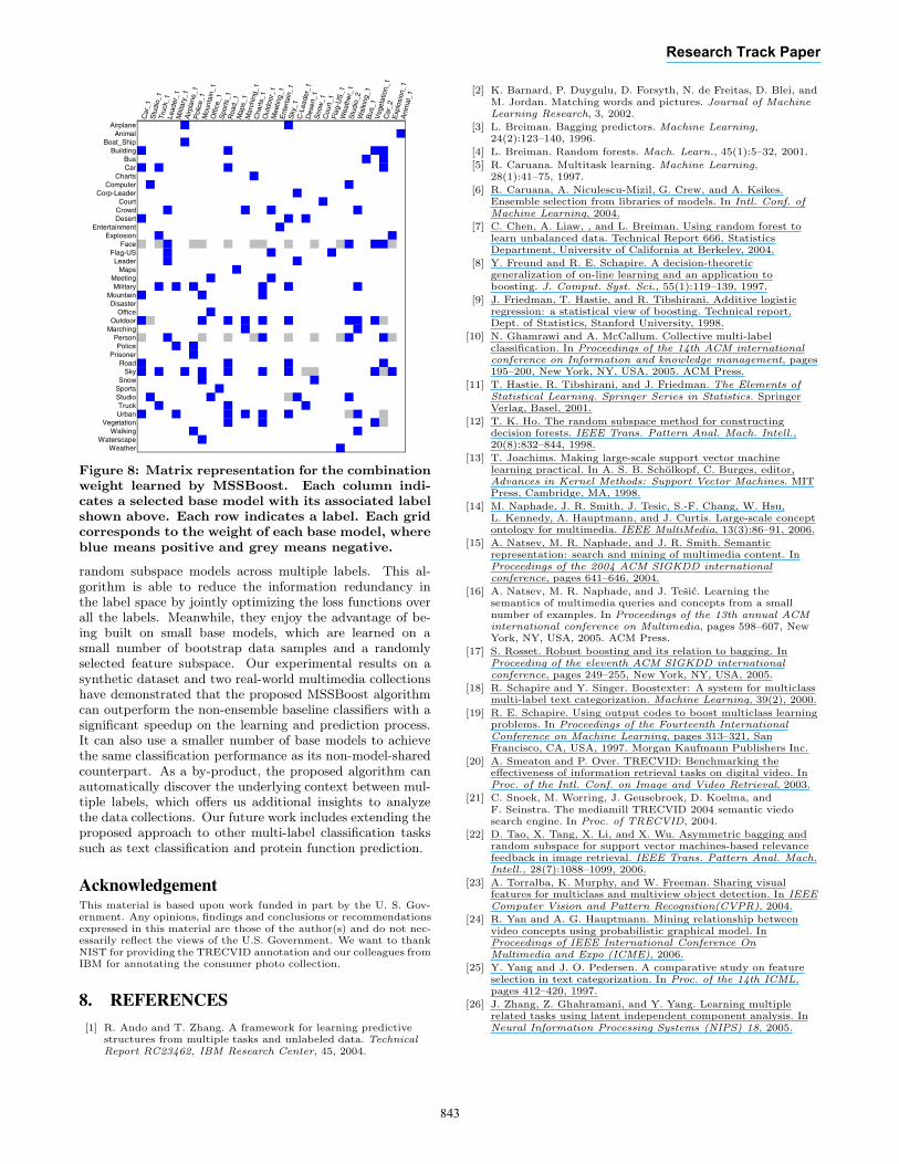
Finally, Figure 8 illustrates the combination weight αtl and

the base models ht for the iteration t from 1 to 30. The se-lected base models in the earliest stage are mostly built fromsome general labels such as “cars”, “studio”, “leader” andso on. A close examination on the other dimension of thematrix indicates that most labels make use of the predic-tions from other related labels. For instance, the label “ur-ban” can benefit from the models of its sub-concepts such as“car”, “road”, “airplane” and so on. On the other hand, thelabel “police” can benefit from its super-concept “military”.These examples shows the advantages of model-sharing fromtwo different perspectives.

7. CONCLUSIONIn this paper, we proposed a boosting-type learning algo-

rithm called model-shared subspace boosting (MSSBoost).It can automatically find, share and combine a number of

Research Track Paper

842

Car

_1S

tudi

o_1

Tru

ck_1

Lead

er_1

Mili

tary

_1A

irpla

ne_1

Pol

ice_

1M

ount

ain_

1O

ffice

_1S

port

s_1

Roa

d_1

Map

s_1

Mar

chin

g_1

Cha

rts_

1O

utdo

or_1

Mee

ting_

1E

nter

tain

_1S

ky_1

C-L

eade

r_1

Des

ert_

1S

now

_1C

ourt

_1F

lag-

US

_1W

eath

er_1

Stu

dio_

2W

alki

ng_1

Bus

_1V

eget

atio

n_1

Car

_2E

xplo

sion

_1A

nim

al_1

AirplaneAnimal

Boat_ShipBuilding

BusCar

ChartsComputer

Corp-LeaderCourt

CrowdDesert

EntertainmentExplosion

FaceFlag-US

LeaderMaps

MeetingMilitary

MountainDisaster

OfficeOutdoor

MarchingPersonPolice

PrisonerRoad

SkySnow

SportsStudioTruckUrban

VegetationWalking

WaterscapeWeather

Figure 8: Matrix representation for the combinationweight learned by MSSBoost. Each column indi-cates a selected base model with its associated labelshown above. Each row indicates a label. Each gridcorresponds to the weight of each base model, whereblue means positive and grey means negative.

random subspace models across multiple labels. This al-gorithm is able to reduce the information redundancy inthe label space by jointly optimizing the loss functions overall the labels. Meanwhile, they enjoy the advantage of be-ing built on small base models, which are learned on asmall number of bootstrap data samples and a randomlyselected feature subspace. Our experimental results on asynthetic dataset and two real-world multimedia collectionshave demonstrated that the proposed MSSBoost algorithmcan outperform the non-ensemble baseline classifiers with asignificant speedup on the learning and prediction process.It can also use a smaller number of base models to achievethe same classification performance as its non-model-sharedcounterpart. As a by-product, the proposed algorithm canautomatically discover the underlying context between mul-tiple labels, which offers us additional insights to analyzethe data collections. Our future work includes extending theproposed approach to other multi-label classification taskssuch as text classification and protein function prediction.

AcknowledgementThis material is based upon work funded in part by the U. S. Gov-ernment. Any opinions, findings and conclusions or recommendationsexpressed in this material are those of the author(s) and do not nec-essarily reflect the views of the U.S. Government. We want to thankNIST for providing the TRECVID annotation and our colleagues fromIBM for annotating the consumer photo collection.

8. REFERENCES[1] R. Ando and T. Zhang. A framework for learning predictive

structures from multiple tasks and unlabeled data. TechnicalReport RC23462, IBM Research Center, 45, 2004.

[2] K. Barnard, P. Duygulu, D. Forsyth, N. de Freitas, D. Blei, andM. Jordan. Matching words and pictures. Journal of MachineLearning Research, 3, 2002.

[3] L. Breiman. Bagging predictors. Machine Learning,24(2):123–140, 1996.

[4] L. Breiman. Random forests. Mach. Learn., 45(1):5–32, 2001.

[5] R. Caruana. Multitask learning. Machine Learning,28(1):41–75, 1997.

[6] R. Caruana, A. Niculescu-Mizil, G. Crew, and A. Ksikes.Ensemble selection from libraries of models. In Intl. Conf. ofMachine Learning, 2004.

[7] C. Chen, A. Liaw, , and L. Breiman. Using random forest tolearn unbalanced data. Technical Report 666, StatisticsDepartment, University of California at Berkeley, 2004.

[8] Y. Freund and R. E. Schapire. A decision-theoreticgeneralization of on-line learning and an application toboosting. J. Comput. Syst. Sci., 55(1):119–139, 1997.

[9] J. Friedman, T. Hastie, and R. Tibshirani. Additive logisticregression: a statistical view of boosting. Technical report,Dept. of Statistics, Stanford University, 1998.

[10] N. Ghamrawi and A. McCallum. Collective multi-labelclassification. In Proceedings of the 14th ACM internationalconference on Information and knowledge management, pages195–200, New York, NY, USA, 2005. ACM Press.

[11] T. Hastie, R. Tibshirani, and J. Friedman. The Elements ofStatistical Learning. Springer Series in Statistics. SpringerVerlag, Basel, 2001.

[12] T. K. Ho. The random subspace method for constructingdecision forests. IEEE Trans. Pattern Anal. Mach. Intell.,20(8):832–844, 1998.

[13] T. Joachims. Making large-scale support vector machinelearning practical. In A. S. B. Scholkopf, C. Burges, editor,Advances in Kernel Methods: Support Vector Machines. MITPress, Cambridge, MA, 1998.

[14] M. Naphade, J. R. Smith, J. Tesic, S.-F. Chang, W. Hsu,L. Kennedy, A. Hauptmann, and J. Curtis. Large-scale conceptontology for multimedia. IEEE MultiMedia, 13(3):86–91, 2006.

[15] A. Natsev, M. R. Naphade, and J. R. Smith. Semanticrepresentation: search and mining of multimedia content. InProceedings of the 2004 ACM SIGKDD internationalconference, pages 641–646, 2004.

[16] A. Natsev, M. R. Naphade, and J. Tesic. Learning thesemantics of multimedia queries and concepts from a smallnumber of examples. In Proceedings of the 13th annual ACMinternational conference on Multimedia, pages 598–607, NewYork, NY, USA, 2005. ACM Press.

[17] S. Rosset. Robust boosting and its relation to bagging. InProceeding of the eleventh ACM SIGKDD internationalconference, pages 249–255, New York, NY, USA, 2005.

[18] R. Schapire and Y. Singer. Boostexter: A system for multiclassmulti-label text categorization. Machine Learning, 39(2), 2000.

[19] R. E. Schapire. Using output codes to boost multiclass learningproblems. In Proceedings of the Fourteenth InternationalConference on Machine Learning, pages 313–321, SanFrancisco, CA, USA, 1997. Morgan Kaufmann Publishers Inc.

[20] A. Smeaton and P. Over. TRECVID: Benchmarking theeffectiveness of information retrieval tasks on digital video. InProc. of the Intl. Conf. on Image and Video Retrieval, 2003.

[21] C. Snoek, M. Worring, J. Geusebroek, D. Koelma, andF. Seinstra. The mediamill TRECVID 2004 semantic viedosearch engine. In Proc. of TRECVID, 2004.

[22] D. Tao, X. Tang, X. Li, and X. Wu. Asymmetric bagging andrandom subspace for support vector machines-based relevancefeedback in image retrieval. IEEE Trans. Pattern Anal. Mach.Intell., 28(7):1088–1099, 2006.

[23] A. Torralba, K. Murphy, and W. Freeman. Sharing visualfeatures for multiclass and multiview object detection. In IEEEComputer Vision and Pattern Recognition(CVPR), 2004.

[24] R. Yan and A. G. Hauptmann. Mining relationship betweenvideo concepts using probabilistic graphical model. InProceedings of IEEE International Conference OnMultimedia and Expo (ICME), 2006.

[25] Y. Yang and J. O. Pedersen. A comparative study on featureselection in text categorization. In Proc. of the 14th ICML,pages 412–420, 1997.

[26] J. Zhang, Z. Ghahramani, and Y. Yang. Learning multiplerelated tasks using latent independent component analysis. InNeural Information Processing Systems (NIPS) 18, 2005.

Research Track Paper

843