DRAFT SUBMITTED TO THE IEEE TRANS ON SPEECH AND AUDIO PROCESSING 2001 1

Generalized Digital Waveguide NetworksDavide Rocchesso Julius O Smith III

Abstractmdash Digital waveguides are generalized to the

multivariable case with the goal of maximizing gen-

erality while retaining robust numerical properties

and simplicity of realization Multivariable complex

power is defined and conditions for ldquomedium pas-

sivityrdquo are presented Multivariable complex wave

impedances such as those deriving from multivari-

able lossy waveguides are used to construct scattering

junctions which yield frequency dependent scattering

coefficients which can be implemented in practice us-

ing digital filters The general form for the scattering

matrix at a junction of multivariable waveguides is

derived An efficient class of loss-modeling filters is

derived including a rule for checking validity of the

small-loss assumption An example application in mu-

sical acoustics is given

I Introduction

Digital Waveguide Networks (DWN) have beenwidely used to develop efficient discrete-time physi-cal models for sound synthesis particularly for wood-wind string and brass musical instruments [1] [2][3] [4] [5] [6] [7] They were initially developed forartificial reverberation [8] [9] [10] and more recentlythey have been applied to robust numerical simula-tion of 2D and 3D vibrating systems [11] [12] [13][14] [15] [16] [17]

A digital waveguide may be thought of as a sam-pled transmission linemdashor acoustic waveguidemdashinwhich sampled unidirectional traveling waves are ex-plicitly simulated Simulating traveling-wave compo-nents in place of physical variables such as pressureand velocity can lead to significant computationalreductions particularly in sound synthesis applica-tions since the models for most traditional musicalinstruments (in the string wind and brass families)can be efficiently simulated using one or two long de-lay lines together with sparsely distributed scatteringjunctions and filters [2] [18] [19] Moreover desir-able numerical properties are more easily ensured inthis framework such as stability [20] ldquopassivityrdquo ofround-off errors and minimized sensitivity to coeffi-

D Rocchesso is with the Dipartimento di Informatica Uni-versita degli Studi di Verona strada Le Grazie 37134 Verona -ITALY Phone ++390458027979 FAX ++390458027982E-mail rocchessosciunivrit J O Smith is with the Cen-ter for Computer Research in Music and Acoustics (CCRMA)Music Department Stanford University Stanford CA 94305E-mail josccrmastanfordedu

cient quantization [21] [22] [23] [14]

In [24] a multivariable formulation of digital wave-guides was proposed in which the real positive char-acteristic impedance of the waveguide medium (beit an electric transmission line or an acoustic tube)is generalized to any q times q para-Hermitian matrixThe associated wave variables were generalized to aqtimesm matrix of z transforms From fundamental con-straints assumed at a junction of two or more wave-guides (pressure continuity conservation of flow) as-sociated multivariable scattering relations were de-rived and various properties were noted

In this paper partially based on [25] we pursue adifferent path to vectorized DWNs starting with amultivariable generalization of the well known tele-

grapherrsquos equations [26] This formulation provides amore detailed physical interpretation of generalizedquantities and new potential applications are indi-cated

The paper is organized as follows Section II in-troduces the generalized DWN formulation startingwith the scalar case and proceeding to the multi-variable case The generalized wave impedance andcomplex signal power appropriate to this formulationare derived and conditions for ldquopassiverdquo computa-tion are given In Section III losses are introducedand some example applications are considered Fi-nally Section IV presents a derivation of the generalform of the physical scattering junctions induced in-tersecting multivariable digital waveguides

II Multivariable DWN Formulation

This section reviews the DWN paradigm andbriefly outlines considerations arising in acoustic sim-ulation applications The multivariable formulationis based on m-dimensional vectors of ldquopressurerdquo andldquovelocityrdquo p and u respectively These variables canbe associated with physical quantities such as acous-tic pressure and velocity respectively or they can beanything analogous such as electrical voltage and cur-rent or mechanical force and velocity We call thesedual variables Kirchhoff variables to distinguish themfrom wave variables [22] which are their traveling-wave components In other words in a 1D waveguidetwo components traveling in opposite directions must

be summed to produce a physical variable For con-creteness we will focus on generalized pressure andvelocity waves in a lossless linear acoustic tube Inacoustic tubes velocity waves are in units of volumevelocity (particle velocity times cross-sectional areaof the tube) [27]

A The Ideal Waveguide

First we address the scalar case For an idealacoustic tube we have the following wave equa-

tion [27]part2p(x t)

partt2= c2 part2p(x t)

partx2 (1)

where p(x t) denotes (scalar) pressure in the tube atthe point x along the tube at time t in seconds If thelength of the tube is LR then x is taken to lie between0 and LR We adopt the convention that x increasesldquoto the rightrdquo so that waves traveling in the directionof increasing x are referred to as ldquoright-goingrdquo Theconstant c is the speed of sound propagation in thetube given by c =

radic

Kmicro where K is the ldquotension1rdquoof the gas in the tube and micro is the mass per unit vol-ume of the tube The dual variable volume velocityu also obeys (1) with p replaced by u The waveequation (1) also holds for an ideal string if p rep-resents the transverse displacement K is the tensionof the string and micro is its linear mass density

The wave equation (1) follows from the more phys-ically meaningful equations [28 p 243]

minuspartp(x t)

partx= micro

partu(x t)

partt(2)

minuspartu(x t)

partx= Kminus1 partp(x t)

partt (3)

Equation (2) follows immediately from Newtonrsquos sec-ond law of motion while (3) follows from conserva-tion of mass and properties of an ideal gas

The general traveling-wave solution to (1) or (2)and (3) was given by DrsquoAlembert as [27]

p(x t) = p+(xminus ct) + pminus(x + ct)u(x t) = u+(xminus ct) + uminus(x + ct)

(4)

where p+ pminus u+ uminus are the right- and left-goingwave components of pressure and velocity respect-ively and are referred to as wave variables Thissolution form is interpreted as the sum of two fixed

1ldquoTensionrdquo is defined here for gases as the reciprocal of theadiabatic compressibility of the gas [28 p 230] This definitionhelps to unify the scattering formalism for acoustic tubes withthat of mechanical systems such as vibrating strings

wave-shapes traveling in opposite directions along thetube The specific waveshapes are determined by theinitial pressure p(x 0) and velocity u(x 0) through-out the tube x isin [0 LR]

B Multivariable Formulation of the Waveguide

Perhaps the most straightforward multivariablegeneralization of (2) and (3) is

partp(x t)

partx= minusM

partu(x t)

partt(5)

partp(x t)

partt= minusK

partu(x t)

partx(6)

in the spatial coordinates xT = [x1 middot middot middot xm] at time

t where M and K are mtimesm non-singular matricesplaying the respective roles of multidimensional massand tension Differentiating (5) with respect to x

and (6) with respect to t and eliminating the termpart2u(x t)partxpartt yields the m-variable generalizationof the wave equation

part2p(x t)

partt2= KMminus1 part2p(x t)

partx2 (7)

The second spatial derivative is defined here as

[

part2p(x t)

partx2

]T=

[

part2p1(x t)

partx21

part2pm(x t)

partx2m

]

(8)Similarly differentiating (5) with respect to t and

(6) with respect to x and eliminating part2p(x t)partxparttyields

part2u(x t)

partt2= Mminus1K

part2u(x t)

partx2 (9)

For digital waveguide modeling we desire solu-tions of the multivariable wave equation involvingonly sums of traveling waves Consider the eigen-function

p(x t) =

est+v1x1

est+vmxm

= estI+V X middot 1 (10)

where s is interpreted as a Laplace-transform vari-able s = σ + jω I is the m times m identity matrix

X=diag(x) V

=diag([v1 vm]) is a diagonal ma-

trix of spatial Laplace-transform variables (the imag-inary part of vi being spatial frequency along the

ith spatial coordinate) and 1T =[1 1] is the m-

dimensional vector of ones Applying the eigenfunc-tion (10) to (7) gives the algebraic equation

s2I = KMminus1V 2 = Cp

2V 2 (11)

2

where Cp is the diagonal matrix of sound-speedsalong the m coordinate axes Since Cp

2V 2 = s2Iwe have

V = plusmnsCp

minus1 (12)

Substituting (12) into (10) the eigensolutions of (7)are found to be of the form

p(x t) = es(

tIplusmnCp

minus1X)

middot 1 (13)

Similarly applying (10) to (9) yields

V = plusmnsCu

minus1 (14)

where Cu

= Mminus1K The eigensolutions of (9) are

then of the form

u(x t) = es(

tIplusmnCu

minus1X)

middot 1 (15)

The generalized sound-speed matrices Cp and Cu arethe same whenever Mminus1 and K commute eg whenthey are both diagonal

Having established that (13) is a solution of (7)when condition (11) holds on the matrices M and Kwe can express the general traveling-wave solution to(7) in both pressure and velocity as

p(x t) = p+ + pminus

u(x t) = u+ + uminus (16)

where p+=f(tI minusCp

minus1X) and f is an arbitrary su-perposition of right-going components of the form

(13) (ie taking the minus sign) and pminus=g(tI +

Cp

minus1X) is similarly any linear combination of left-going eigensolutions from (13) (all having the plussign) Similar definitions apply for u+ and uminusWhen the time and space arguments are dropped asin the right-hand side of (16) it is understood thatall the quantities are written for the same time t andposition x

When the mass and tension matrices M and K

are diagonal our analysis corresponds to consideringm separate waveguides as a whole For example thetwo transversal planes of vibration in a string canbe described by (7) with m = 2 In a musical in-strument such as the piano [29] the coupling amongthe strings and between different vibration modali-ties within a single string occurs primarily at thebridge [30] Indeed the bridge acts like a junction ofseveral multivariable waveguides (see section IV)

When the matrices M and K are non-diagonalthe physical interpretation can be of the form

Cp

2 = KMminus1 (17)

where K is the stiffness matrix and M is the mass

density matrix Cp is diagonal if (11) holds andin this case the wave equation (7) is decoupled inthe spatial dimensions There are physical exampleswhere the matrices M and K are not diagonal eventhough (17) is satisfied with a diagonal Cp Onesuch example in the domain of electrical variables isgiven by m conductors in a sheath or above a groundplane where the sheath or the ground plane acts asa coupling element [31 pp 67ndash68] In acoustics itis more common to have coupling introduced by adissipative term in equation (7) but the solution canstill be expressed as decoupled attenuating travelingwaves An example of such acoustical systems willbe presented in Section III-B

Besides the existence of physical systems that sup-port multivariable traveling wave solutions there areother practical reasons for considering a multivari-able formulation of wave propagation For instancemodal analysis considers the vector p (whose dimen-sion is infinite in general) of coefficients of the normalmode expansion of the system response For spacesin perfectly reflecting enclosures p can be compactedso that each element accounts for all the modes shar-ing the same spatial dimension [32] p admits a wavedecomposition as in (16) and Cp is diagonal Havingwalls with finite impedance there is a damping termproportional to partppartt that functions as a couplingterm among the ideal modes [33] Coupling amongthe modes can also be exerted by diffusive propertiesof the enclosure [32] [9]

Note that the multivariable wave equation (7) con-sidered here does not include wave equations govern-ing propagation in multidimensional media (such asmembranes spaces and solids) In higher dimen-sions the solution in the ideal linear lossless case isa superposition of waves traveling in all directions

in the m-dimensional space [27] However it turnsout that a good simulation of wave propagation ina multidimensional medium may in fact be obtainedby forming a mesh of unidirectional waveguides asconsidered here each described by (7) such a meshof 1D waveguides can be shown to solve numericallya discretized wave equation for multidimensional me-dia [34] [35] [13] [14]

3

where Cp is the diagonal matrix of sound-speedsalong the m coordinate axes Since Cp

2V 2 = s2Iwe have

V = plusmnsCp

minus1 (12)

Substituting (12) into (10) the eigensolutions of (7)are found to be of the form

p(x t) = es(

tIplusmnCp

minus1X)

middot 1 (13)

Similarly applying (10) to (9) yields

V = plusmnsCu

minus1 (14)

where Cu

= Mminus1K The eigensolutions of (9) are

then of the form

u(x t) = es(

tIplusmnCu

minus1X)

middot 1 (15)

The generalized sound-speed matrices Cp and Cu arethe same whenever Mminus1 and K commute eg whenthey are both diagonal

Having established that (13) is a solution of (7)when condition (11) holds on the matrices M and Kwe can express the general traveling-wave solution to(7) in both pressure and velocity as

p(x t) = p+ + pminus

u(x t) = u+ + uminus (16)

where p+=f(tI minusCp

minus1X) and f is an arbitrary su-perposition of right-going components of the form

(13) (ie taking the minus sign) and pminus=g(tI +

Cp

minus1X) is similarly any linear combination of left-going eigensolutions from (13) (all having the plussign) Similar definitions apply for u+ and uminusWhen the time and space arguments are dropped asin the right-hand side of (16) it is understood thatall the quantities are written for the same time t andposition x

When the mass and tension matrices M and K

are diagonal our analysis corresponds to consideringm separate waveguides as a whole For example thetwo transversal planes of vibration in a string canbe described by (7) with m = 2 In a musical in-strument such as the piano [29] the coupling amongthe strings and between different vibration modali-ties within a single string occurs primarily at thebridge [30] Indeed the bridge acts like a junction ofseveral multivariable waveguides (see section IV)

When the matrices M and K are non-diagonalthe physical interpretation can be of the form

Cp

2 = KMminus1 (17)

where K is the stiffness matrix and M is the mass

density matrix Cp is diagonal if (11) holds andin this case the wave equation (7) is decoupled inthe spatial dimensions There are physical exampleswhere the matrices M and K are not diagonal eventhough (17) is satisfied with a diagonal Cp Onesuch example in the domain of electrical variables isgiven by m conductors in a sheath or above a groundplane where the sheath or the ground plane acts asa coupling element [31 pp 67ndash68] In acoustics itis more common to have coupling introduced by adissipative term in equation (7) but the solution canstill be expressed as decoupled attenuating travelingwaves An example of such acoustical systems willbe presented in Section III-B

Besides the existence of physical systems that sup-port multivariable traveling wave solutions there areother practical reasons for considering a multivari-able formulation of wave propagation For instancemodal analysis considers the vector p (whose dimen-sion is infinite in general) of coefficients of the normalmode expansion of the system response For spacesin perfectly reflecting enclosures p can be compactedso that each element accounts for all the modes shar-ing the same spatial dimension [32] p admits a wavedecomposition as in (16) and Cp is diagonal Havingwalls with finite impedance there is a damping termproportional to partppartt that functions as a couplingterm among the ideal modes [33] Coupling amongthe modes can also be exerted by diffusive propertiesof the enclosure [32] [9]

Note that the multivariable wave equation (7) con-sidered here does not include wave equations govern-ing propagation in multidimensional media (such asmembranes spaces and solids) In higher dimen-sions the solution in the ideal linear lossless case isa superposition of waves traveling in all directions

in the m-dimensional space [27] However it turnsout that a good simulation of wave propagation ina multidimensional medium may in fact be obtainedby forming a mesh of unidirectional waveguides asconsidered here each described by (7) such a meshof 1D waveguides can be shown to solve numericallya discretized wave equation for multidimensional me-dia [34] [35] [13] [14]

3

C Multivariable Wave Impedance

From (5) we have using (13)

partp(x t)partx = minusMpartu(x t)parttrArr plusmnsCp

minus1p = minussMu

rArr p = plusmnCpMu

= plusmnK12M12u= plusmnRu

(18)

where lsquo+rsquo is for right-going and lsquominusrsquo is for left-goingThus following the classical definition for the scalarcase the mtimesm wave impedance is defined by

R= K12M12 = CpM = KCu (19)

and we have

p+ = Ru+

pminus = minus Ruminus (20)

Thus the wave impedance R is the factor of propor-tionality between pressure and velocity in a travelingwave In the cases governed by the ideal wave equa-tion (7) R is diagonal if and only if the mass matrixM is diagonal (since Cp is assumed diagonal) Theminus sign for the left-going wave pminus accounts for thefact that velocities must move to the left to generatepressure to the left The wave admittance is definedas Γ = Rminus1

A linear propagation medium in the discrete-timecase is completely determined by its wave impedance

R(zx) which in a generalized formulation is fre-quency dependent and spatially varying Examplesof such general cases will be given in the sectionsthat follow A waveguide is defined for purposes ofthis paper as a length of medium in which the waveimpedance is either constant with respect to spatialposition x or else it varies smoothly with x in sucha way that there is no scattering (as in the coni-cal acoustic tube2) For simplicity we will suppressthe possible spatial dependence and write only R(z)which is intended to be an m times m function of thecomplex variable z analytic for |z| gt 1

2There appear to be no tube shapes supporting exact travel-ing waves other than cylindrical and conical (or conical wedgewhich is a hybrid) [36] However the ldquoSalmon horn familyrdquo(see eg [27] [37]) characterizes a larger class of approximateone-parameter traveling waves In the cone the wave equationis solved for pressure p(x t) using a change of variables pprime = pxwhere x is the distance from the apex of the cone causing thewave equation for the cone pressure to reduce to the cylindri-cal case [38] Note that while pressure waves behave simplyas non-dispersive traveling waves in cones the correspondingvelocity waves are dispersive [38]

The generalized version of (20) is

p+ = R(z)u+

pminus = minus Rlowast(1zlowast)uminus (21)

where Rlowast(1zlowast) is the paraconjugate of R(z) ie theunique analytic continuation (when it exists) fromthe unit circle to the complex plane of the conjugatetransposed of R(z) [39]

D Multivariable Complex Signal Power

The net complex power involved in the propagationcan be defined as [40]

P = ulowastp = (u+ + uminus)lowast(p+ + pminus)

= u+lowastRu+ minus uminuslowast

Rlowastuminus +

uminuslowastRu+ minus u+lowast

Rlowastuminus

= (P+ minus Pminus) + (Ptimes minus Ptimeslowast) (22)

where all quantities above are functions of z asin (21) The quantity P+ = u+lowast

Ru+ is called right-

going active power (or right-going average dissipatedpower3) while Pminus = uminuslowast

Rlowastuminus is called the left-

going active power The term P+ minus Pminus the right-going minus the left-going power components we callthe net active power while the term PtimesminusPtimeslowast is net

reactive power These names all stem from the case inwhich the matrix R(z) is positive definite for |z| ge 1In this case both the components of the active powerare real and positive the active power itself is realwhile the reactive power is purely imaginary

E Medium Passivity

Following the classical definition of passivity [40][41] a medium is said to be passive if

ReP+ + Pminus ge 0 (23)

for |z| ge 1 Thus a sufficient condition for ensuringpassivity in a medium is that each traveling active-power component is real and non-negative

To derive a definition of passivity in terms of thewave impedance consider a perfectly reflecting inter-ruption in the transmission line such that uminus = u+

3Note that |z| = 1 corresponds to the average physical powerat frequency ω where z = exp(jωT ) and the wave variablemagnitudes on the unit circle may be interpreted as RMS lev-els For |z| gt 1 we may interpret the power u

lowast(1zlowast)p(z) asthe steady state power obtained when exponential damping isintroduced into the waveguide giving decay time-constant τ where z = exp(minusTτ) exp(jωT ) (for the continuous-time casesee [40 p 48])

4

For a passive medium using (22) the inequality (23)becomes

R(z) + Rlowast(1zlowast) ge 0 (24)

for |z| ge 1 Ie the sum of the wave impedance andits paraconjugate is positive semidefinite

The wave impedance R(z) is an m-by-m functionof the complex variable z Condition (24) is essen-tially the same thing as saying R(z) is positive real4

[42] except that it is allowed to be complex even forreal z

The matrix Rlowast(1zlowast) is the paraconjugate of R

Since Rlowast(1zlowast) generalizes R(ejω)T to the entire

complex plane we may interpret [R(z)+Rlowast(1zlowast)]2as generalizing the Hermitian part of R(z) to the z-plane viz the para-Hermitian part

Since the inverse of a positive-real function is pos-itive real the corresponding generalized wave admit-tance Γ(z) = Rminus1(z) is positive real (and hence an-alytic) in |z| ge 1

We say that wave propagation in the medium islossless if the impedance matrix is such that

R(z) = Rlowast(1zlowast) (25)

ie if R(z) is para-Hermitian (which implies its in-verse Γ(z) is also)

Most applications in waveguide modeling are con-cerned with nearly lossless propagation in passive me-dia In this paper we will state results for R(z) inthe more general case when applicable while con-sidering applications only for constant and diagonalimpedance matrices R As shown in Section II-Ccoupling in the wave equation (7) implies a non-diagonal impedance matrix since there is usually aproportionality between the speed of propagation Cp

and the impedance R through the non-diagonal ma-trix M (see eq 19)

F Multivariable Digital Waveguides

The wave components of equations (16) travelundisturbed along each axis This propagation is im-plemented digitally using m bidirectional delay linesas depicted in Fig 1 We call such a collection ofdelay lines an m-variable waveguide section Wave-guide sections are then joined at their endpoints viascattering junctions (discussed in section IV) to forma DWN

4A complex-valued function of a complex variable f(z) issaid to be positive real if1) z real rArr f(z) real2) |z| ge 1 rArr Ref(z) ge 0Positive real functions characterize passive impedances in clas-sical network theory

p (t)+

z-mL

z-m

L

p (t + m T)-

+p (t - m T)

L s

L s

p (t)-

p (t)+

z-mL

z-m

L

p (t + m T)-

+p (t - m T)

L s

L s

p (t)-

1 1

11

m

m

m

m

Fig 1

An m-variable waveguide section

III Lossy Waveguides

A Multivariable Formulation

The m-variable lossy wave equation is

part2p(x t)

partt2+KMminus1ΦKminus1 partp(x t)

partt= KMminus1 part2p(x t)

partx2

(26)where Φ is a mtimesm matrix that represents a viscousresistance If we plug the eigensolution (10) into (26)we get in the Laplace domain

s2I + sKMminus1ΦKminus1 = KMminus1V 2 = Cp

2V 2 (27)

or by letting

ΦKminus1 = Υ (28)

we gets2I + sCp

2Υ = Cp

2V 2 (29)

By restricting the Laplace analysis to the imaginary(frequency) axis s = jωs decomposing the (diagonal)spatial frequency matrix into its real and imaginaryparts V = V R + jV I and equating the real andimaginary parts of equation (29) we get the equa-tions

V R2 minus V I

2 = minusCp

minus2ωs (30)

2V RV I = ωsΥ (31)

The term V R can be interpreted as attenuation perunit length while V I keeps the role of spatial fre-quency so that the traveling wave solution is

p = eV RXej(ωstIminusV IX) middot 1 (32)

Defining Θ as the ratio5 between the real and imag-inary parts of V (ΘV I = V R) the equations (30)

5Indeed in the general case Θ is a diagonal matrix

5

and (31) become

V 2I =

(

I minusΘ2)minus1

ωs2Cp

minus2 (33)

Υ = 2Θ(

I minusΘ2)minus1

ωsCp

minus2 (34)

Following steps analogous to those of eq (18) themtimesm admittance matrix turns out to be

Γ = Mminus1(

I minusΘ2)minus12

Cp

minus1 minus1

sMminus1V R (35)

which for Φrarr 0 collapses to the reciprocal of (19)For the discrete-time case we may map Γ(sx) fromthe s plane to the z plane via the bilinear transfor-mation [43] or we may sample the inverse Laplacetransform of Γ(sx) and take its z transform to ob-

tain Γ(zx)

B Example in Acoustics

There are examples of acoustics systems made oftwo or more tightly coupled media whose wave prop-agation can be simulated by a multivariable wave-guide section One such system is an elastic poroussolid [28 pp 609ndash611] where the coupling betweengas and solid is given by the frictional force arisingwhen the velocities in the two media are not equalThe wave equation for this acoustic system is (26)where the matrix Φ takes form

Φ =

[

Φ minusΦminusΦ Φ

]

(36)

and Φ is a flow resistance The stiffness and the massmatrices are diagonal and can be written as

K =

[

ka 00 kb

]

(37)

M =

[

microa 00 microb

]

(38)

Let us try to enforce a traveling wave solution withspatial and temporal frequencies V and ωs respect-ively

p = p0ej(V xminusωst) =

[

pa

ps

]

(39)

where pa and ps are the pressure wave componentsin the gas and in the solid respectively We easilyobtain from (26) the two relations

jωsΦksminus1ps = (ωs

2αa2 minus V 2)pa (40)

jωsΦkaminus1pa = (ωs

2αs2 minus V 2)ps (41)

where

αa2 = ca

minus2 + jksΦ

ω(42)

αs2 = cs

minus2 + jkaΦ

ω(43)

and ca and cs are the sound speeds in the gas and inthe solid respectively By multiplying together bothmembers of (40) and (41) we get

V 2 = 12ωs

2(αa2 + αs

2)plusmn12

radic

ωs4(αa

2 minus αs2)2 minus 4ωs

2Φ2kakb(44)

Equation (44) gives us a couple of complex numbersfor v ie two attenuating traveling waves forminga vector p as in (32) It can be shown [28 p 611]that in the case of small flow resistance the fasterwave propagates at a speed slightly slower than csand the slower wave propagates at a speed slightlyfaster than ca It is also possible to show that theadmitance matrix (35) is non-diagonal and frequencydependent

This example is illustrative of cases in which thematrices K and M are diagonal and the couplingamong different media is exerted via the resistancematrix Φ If Φ approaches zero we are back to thecase of decoupled waveguides In any case two pairsof delay lines are adequate to model this kind of sys-tem

C Lossy Digital Waveguides

Let us now approach the simulation of propaga-tion in lossy media which are represented by equa-tion (26) We treat the one-dimensional scalar casehere in order to focus on the kinds of filters thatshould be designed to embed losses in digital wave-guide networks [44] [25]

As usual by inserting the exponential eigensolu-tion into the wave equation we get the one-variableversion of (29)

s2

c2+ sΥ = V 2 (45)

where V is the wave number or spatial frequencyand it represents the wave length and attenuation inthe direction of propagation

Reconsidering the treatment of section III-A andreducing it to the scalar case let us derive from (33)and (34) the expression for Θ

Θ =1

2Υωs|VI |

minus2 (46)

6

which gives the unique solution for (33)

Θ = minusωs

Υc2+

radic

ωs2

Υ2c4+ 1 (47)

This shows us that the exponential attenuationin (32) is frequency dependent and we can even plotthe real and imaginary parts of the wave number Vas functions of frequency as reported in Fig 2

0 100 200 300 400 500 600 700 800 900 10000

5

10

15

20

frequency (Hz)

Im(V

)

wavenumber vs frequency (loss coefficient = 0001)

0 100 200 300 400 500 600 700 800 900 1000005

01

015

02

frequency (Hz)

Re(

V)

Fig 2

Imaginary and real part of the wave number as

functions of frequency (Υ = 0001)

If the frequency range of interest is above a certainthreshold ie Υc2ωs is small we can obtain thefollowing relations from (47) by means of a Taylorexpansion truncated at the first term

|vI | ≃ωs

c

|vR| ≃12Υc

(48)

Namely for sufficiently high frequencies the attenu-ation can be considered to be constant and the dis-persion relation can be considered to be the same asin a non-dissipative medium as it can be seen fromFig 2

Still under the assumption of small losses andtruncating the Taylor expansion of Θ to the firstterm we find that the wave admittance (35) reducesto the two ldquodirectional admittancesrdquo

Γ+ = Γ(s) = u+

p+ = G0

(

1 + 1sL

)

Γminus = minusΓlowast(minusslowast) = uminus

pminus= G0

(

minus1 + 1sL

)

(49)

where G0 = 1microc is the admittance of the medium

without losses and L = minus 2Υc2 is a negative shunt

reactance that accounts for losses

The actual wave admittance of a one-dimensionalmedium such as a tube is Γ(s) while Γlowast(minusslowast) is itsparaconjugate in the analog domain Moving to thediscrete-time domain by means of a bilinear transfor-mation it is easy to verify that we get a couple of ldquodi-rectional admittancesrdquo that are related through (21)

In the case of the dissipative tube as we ex-pect wave propagation is not lossless since R(s) 6=Rlowast(minusslowast) However the medium is passive in thesense of section II-E since the sum R(s) + Rlowast(minusslowast)is positive semidefinite along the imaginary axis

The relations here reported hold for any one-dimensional resonator with frictional losses There-fore they hold for a certain class of dissipative stringsand tubes Remarkably similar wave admittances arealso found for spherical waves propagating in conicaltubes (see Appendix A)

The simulation of a length-LR section of lossy res-onator can proceed according to two stages of ap-proximation If the losses are small (ie Υ asymp 0)the approximation (48) can be considered valid in allthe frequency range of interest In such case we canlump all the losses of the section in a single coeffi-cient gL = e

12ΥcLR The resonator can be simulated

by the structure of Fig 3 where we have assumedthat the length LR is equal to an integer number mL

of spatial samples

p (t)+

p (t)+

p (t)-

gL

z-m

z-m

z

z

p(t0) p(tL )

gL

L

L

R

Fig 3

Length-LR one-variable waveguide section with small

losses

At a further level of approximation if the values ofΥ are even smaller we can consider the reactive com-ponent of the admittance to be zero thus assumingΓ+ = Γminus = G0

On the other hand if losses are significant we haveto represent wave propagation in the two directionswith a filter whose frequency response can be deducedfrom Fig 2 In practice we have to insert a filter GL

having magnitude and phase delay that are repre-sented in Fig 4 for different values of Υ From suchfilter we can subtract a contribution of linear phasewhich can be implemented by means of a pure delay

7

0 100 200 300 400 500 600 700 800 900 10000

0005

001

0015

002

frequency (Hz)

phas

e de

lay

amplitude and phase delay Vs frequency

0001

001

01

0 100 200 300 400 500 600 700 800 900 10000

02

04

06

08

1

frequency (Hz)

ampl

itude

0001

001

01

Fig 4

Magnitude and phase delay introduced by frictional

losses in a waveguide section of length LR = 1 for

different values of Υ

C1 An Efficient Class of Loss Filters

A first-order IIR filter that when cascaded witha delay line simulates wave propagation in a lossyresonator of length LR can take the form

GL(z) =

(

α1minus r

1minus rzminus1+ (1minus α)

)

zminusLRFsc

= HL(z)zminusLRFsc (50)

At the Nyquist frequency and for r ≃ 1 such fil-ter gains GL(ejπ) ≃ 1 minus α and we have to use

α = 1 minus eminus12ΥcLR to have the correct attenuation

at high frequency Fig 5 shows the magnitude andphase delay (in seconds) obtained with the first-orderfilter GL for three values of its parameter r

By comparison of the curves of Fig 4 with the re-sponses of Fig 5 we see how the latter can be usedto represent the losses in a section of one-dimensionalwaveguide section Therefore the simulation schemeturns out to be that of Fig 6 Of course better ap-proximations of the curves of Fig 4 can be obtainedby increasing the filter order or at least by control-ling the zero position of a first-order filter How-ever the form (50) is particularly attractive becauseits low-frequency behavior is controlled by the singleparameter r

As far as the wave impedance is concerned in thediscrete-time domain it can be represented by a dig-ital filter obtained from (49) by bilinear transforma-

0 100 200 300 400 500 600 700 800 900 10000

0005

001

0015

002

frequency (Hz)

phas

e de

lay

amplitude and phase delay Vs frequency

099994

09997

09996

0 100 200 300 400 500 600 700 800 900 10000

02

04

06

08

1

frequency (Hz)

ampl

itude

099994

09997

09996

Fig 5

Magnitude and phase delay of a first-order IIR filter

for different values of the coefficient r α is set to

1 minus eminus12ΥcLR with the same values of Υ used for the

curves in fig 4

p (t)+

LH

LH

p (t)+

LH

LH

p (t)+

p (t)-

z-m

z-m

L

L

z-m

z-m

L

L

z

z

H

H

p(t0) p(tL )R

Fig 6

Length-LR one-variable waveguide section with small

losses

tion which leads to

R+ =2LFs

G0

1minus zminus1

2LFs + 1minus (2LFs minus 1)zminus1 (51)

that is a first-order high-pass filter The discretiza-tion by impulse invariance can not be applied in thiscase because the impedance has a high-frequency re-sponse that would alias heavily

C2 Validity of Small-Loss Approximation

One might ask how accurate are the small-loss ap-proximations leading to (48) We can give a quanti-tative answer by considering the knee of the curve inFig 4 and saying that we are in the small-losses caseif the knee is lower than the lowest modal frequencyof the resonator Given a certain value of frictionΥ we can find the best approximating IIR filter andthen find its knee frequency ωk corresponding to amagnitude that is 1 + d times the asymptotic value

8

with d a small positive number If such frequency ωkis smaller than the lowest modal frequency we cantake the small-losses assumption as valid and use thescheme of fig 3

C3 Frequency-Dependent Friction

With a further generalization we can considerlosses that are dependent on frequency so that thefriction coefficient Υ is replaced by Υ(ωs) In suchcase all the formulas up to (49) will be recomputedwith this new Υ(ωs)

Quite often losses are deduced from experimentaldata which give the value VR(ωs) In these cases itis useful to calculate the value of Υ(ωs) so that thewave admittance can be computed From (33) wefind

Θ =|VR|

radic

ω2s

c2 + VR2

(52)

and therefore from (46) we get

Υ(ωs) =2|VR(ωs)|

ωs

radic

ω2s

c2+ VR(ωs)

2 (53)

For instance in a radius-a cylindrical tube thevisco-thermal losses can be approximated by the for-mula [45]

|VR(ωs)| =30times 10minus5

a

radic

ωs

2π (54)

which can be directly replaced into (53)In vibrating strings the viscous friction with air

determines a damping that can be represented by theformula [45]

|VR(ωs)| = a1

radic

ωs

2π+ a2 (55)

where a1 and a2 are coefficients that depend on radiusand density of the string

IV Multivariable Waveguide Junctions

A set of N waveguides can be joined together atone of their endpoints to create an N -port waveguide

junction General conditions for lossless scattering inthe scalar case appeared in [9] Waveguide junctionsare isomorphic to adaptors as used in wave digitalfilters [22]

This section focuses on physically realizable scat-tering junctions produced by connecting multivari-able waveguides having potentially complex wave

impedances A physical junction can be realized as aparallel connection of waveguides (as in the connec-tion of N tubes that share the same value of pressureat one point) or as a series connection (as in theconnection of N strings that share the same value ofvelocity at one point) The two kinds of junctions areduals of each other and the resulting matrices sharethe same structure exchanging impedance and ad-mittance Therefore we only treat the parallel junc-tion

A Parallel Junction of Multivariable Complex

Waveguides

We now consider the scattering matrix for the par-allel junction of N m-variable physical waveguidesand at the same time we treat the generalized caseof matrix transfer-function wave impedances Equa-tions (21) and (16) can be rewritten for each m-variable branch as

u+i = Γi(z)p+

i

uminus

i = minusΓlowast

i (1zlowast)pminus

i (56)

andui = u+

i + uminus

i

pi = p+i + pminus

i = pJ1 (57)

where Γi(z) = Rminus1i (z) pJ is the pressure at the junc-

tion and we have used pressure continuity to equatepi to pJ for any i

Using conservation of velocity we obtain

0 = 1TNsum

i=1

ui

= 1TNsum

i=1

[Γi(z) + Γlowast

i (1zlowast)] p+i

minusΓlowast

i (1zlowast)pJ1 (58)

and

pJ = S1TNsum

i=1

[Γi(z) + Γlowast

i (1zlowast)] p+i (59)

where

S =

1T

[

Nsum

i=1

Γlowast

i (1zlowast)

]

1

minus1

(60)

From (57) we have the scattering relation

pminus =

pminus

1pminus

N

= Ap+

9

= A

p+1

p+

N

= pJ

11

minus p+ (61)

where the scattering matrix is deduced from (59)

A = S

1T[

Γ1 + Γlowast

1 ΓN + Γlowast

N

]

1T[

Γ1 + Γlowast

1 ΓN + Γlowast

N

]

minus I

(62)If the branches do not all have the same dimen-

sionality m we may still use the expression (62) byletting m be the largest dimensionality and embed-ding each branch in an m-variable propagation space

B Loaded Junctions

In discrete-time modeling of acoustic systems it isoften useful to attach waveguide junctions to exter-nal dynamic systems which act as a load We speakin this case of a loaded junction [24] The load isexpressed in general by its complex admittance andcan be considered a lumped circuit attached to thedistributed waveguide network

To derive the scattering matrix for the loaded par-allel junction of N lossless acoustic tubes the Kirch-hoffrsquos node equation is reformulated so that the sumof velocities meeting at the junction equals the exitvelocity (instead of zero) For the series junction oftransversely vibrating strings the sum of forces ex-erted by the strings on the junction is set equal tothe force acting on the load (instead of zero)

The load admittance ΓL is regarded as a lumped

driving-point admittance [42] and the equation

UL(z) = ΓL(z)pJ(z) (63)

expresses the relation at the loadFor the general case of N m-variable physical wave-

guides the expression of the scattering matrix is thatof (62) with

S =

[

1T

(

Nsum

i=1

Γi

)

1 + ΓL

]minus1

(64)

C Example in Acoustics

As an application of the theory developed hereinwe outline the digital simulation of two pairs of pi-ano strings The strings are attached to a commonbridge which acts as a coupling element betweenthem (see Fig 7) An in-depth treatment of coupledstrings can be found in [30]

To a first approximation the bridge can be mod-eled as a lumped mass-spring-damper system whilefor the strings a distributed representation as wave-guides is more appropriate For the purpose of illus-trating the theory in its general form we representeach pair of strings as a single 2-variable waveguideThis approach is justified if we associate the pair withthe same key in such a way that both the strings aresubject to the same excitation Actually the 2 times 2matrices M and T of (7) can be considered to bediagonal in this case thus allowing a description ofthe system as four separate scalar waveguides

mz

z

microk

1

2

Fig 7

Two pairs of strings coupled at a bridge

The ith pair of strings is described by the 2-variableimpedance matrix

Ri =

[

Ri1 00 Ri2

]

(65)

The lumped elements forming the bridge are con-nected in series so that the driving-point velocity6 uis the same for the spring mass and damper

u(t) = um(t) = uk(t) = umicro(t) (66)

Also the forces provided by the spring mass anddamper add

p(t) = pm(t) + pk(t) + pmicro(t) (67)

We can derive an expression for the bridgeimpedances using the following relations in the

6The symbols for the variables velocity and force have beenchosen to maintain consistency with the analogous acousticalquantities

10

Laplace-transform domain

Pk(s) = (ks)Uk(s)Pm(s) = msUm(s)Pmicro(s) = microUmicro(s)

(68)

Equations (68) and (67) give the continuous-timeload impedance

RL(s) =P (s)

U(s)= m

s2 + smicrom + km

s (69)

In order to move to the discrete-time domain we mayapply the bilinear transform

slarr α1minus zminus1

1 + zminus1(70)

to (69) The factor α is used to control the compres-sion of the frequency axis It may be set to 2T sothat the discrete-time filter corresponds to integrat-ing the analog differential equation using the trape-zoidal rule or it may be chosen to preserve the reso-nance frequency

We obtain

RL(z) =[

(α2 minus αmicrom + km)zminus2

+ (minus2α2 + 2km)zminus1

+ (α2 + αmicrom + km)] [

αm(1minus zminus2)]

The factor S in the impedance formulation of thescattering matrix (62) is given by

S(z) =

2sum

ij=1

Rij + RL(z)

minus1

(71)

which is a rational function of the complex variablez The scattering matrix is given by

A = 2S

R11 R12 R21 R22

R11 R12 R21 R22

R11 R12 R21 R22

R11 R12 R21 R22

minus I (72)

which can be implemented using a single second-order filter having transfer function (71)

V Conclusions

We presented a generalized formulation of digitalwaveguide networks derived from a vectorized setof telegrapherrsquos equations Multivariable complexpower was defined and conditions for ldquomedium pas-sivityrdquo were presented Incorporation of losses was

carried out and applications were discussed An ef-ficient class of loss-modeling filters was derived anda rule for checking validity of the small-loss assump-tion was proposed Finally the form of the scatter-ing matrix was derived in the case of a junction ofmultivariable waveguides and an example in musicalacoustics was given

Appendix

I Propagation of Spherical Waves (ConicalTubes)

We have seen how a tract of cylindrical tube is gov-erned by a partial differential equation such as (7)and therefore it admits exact simulation by meansof a waveguide section When the tube has a con-ical profile the wave equation is no longer (1) butwe can use the equation for propagation of sphericalwaves [27]

1

r2

part

partr

(

r2 partp(r t)

partr

)

=1

c2

part2p(r t)

partt2 (73)

where r is the distance from the cone apexIn the equation (73) we can evidentiate a term in

the first derivative thus obtaining

part2p(r t)

partr2+

2

r

partp(r t)

partr=

1

c2

part2p(r t)

partt2 (74)

If we recall equation (26) for lossy waveguides wefind some similarities Indeed we are going to showthat in the scalar case the media described by (26)and (74) have structurally similar wave admittances

Let us put a complex exponential eigensolutionin (73) with an amplitude correction that accountsfor energy conservation in spherical wavefronts Sincethe area of such wavefront is proportional to r2 suchamplitude correction has to be inversely proportionalto r in such a way that the product intensity (thatis the square of amplitude) by area is constant Theeigensolution is

p(r t) =1

rest+vr (75)

where s is the complex temporal frequency and vis the complex spatial frequency By substitutionof (75) in (73) we find the algebraic relation

v = plusmns

c (76)

So even in this case the pressure can be expressedby the first of (4) where

p+ = 1r es(tminusrc) pminus = 1

r es(t+rc) (77)

11

Newtonrsquos second law

partur

partt= minus

1

ρ

partp

partr(78)

applied to (77) allows to express the particle velocityur as

ur(r t) =

(

1

rs∓

1

c

)

1

ρres(tplusmnrc) (79)

Therefore the two wave components of the air floware given by

u+ = S(

1rs + 1

c

)

1ρr es(tminusrc)

uminus = S(

1rs minus

1c

)

1ρr es(t+rc)

(80)

where S is the area of the spherical shell outlined bythe cone at point r

We can define the two wave admittances

Γ+ = Γ(s) = u+

p+ = G0

(

1 + 1sL

)

Γminus = minusΓlowast(minusslowast) = uminus

pminus= G0

(

minus1 + 1sL

)

(81)

where G0 = Sρc is the admittance in the degenerate

case of a null tapering angle and L = rc is a shunt

reactance accounting for conicity [46] The wave ad-mittance for the cone is Γ(s) and Γlowast(minusslowast) is its para-conjugate in the analog domain If we translate theequations into the discrete-time domain by bilineartransformation we can check the validity of equa-tions (21) for the case of the cone

Wave propagation in conical ducts is not losslesssince R(s) 6= Rlowast(minusslowast) However the medium ispassive in the sense of section II since the sumR(s) + Rlowast(minusslowast) is positive semidefinite along theimaginary axis

As compared to the lossy cylindrical tube theexpression for wave admittance is structurally un-changed with the only exception of the sign inversionin the shunt inductance This difference is justifiedby thinking of the shunt inductance as a representa-tion of the signal that does not propagate along thewaveguide In the case of the lossy tube such sig-nal is dissipated into heat in the case of the cone itfills the shell that is formed by interfacing a planarwavefront with a spherical wavefront

The discrete-time simulation of a length-LR conetract having the (left) narrow end at distance r0 fromthe apex is depicted in figure 8

References

[1] J O Smith ldquoEfficient simulation of the reed-bore andbow-string mechanismsrdquo in Proc 1986 Int Computer

p (t)+

p (t)+

p (t)-

-mz

r0r

r0

r0

r0

z

z-m

L

L

-1R 0(L + )

Rp(t + L )

0p(tr )

Fig 8

One-variable waveguide section for a length-LR

conical tract

Music Conf The Hague pp 275ndash280 Computer MusicAssociation 1986 Also available in [24]

[2] J O Smith ldquoPhysical modeling using digital wave-guidesrdquo Computer Music J vol 16 pp 74ndash91Winter 1992 Special issue Physical Modelingof Musical Instruments Part I Available online athttpccrmastanfordedu˜jos

[3] V Valimaki and M Karjalainen ldquoImproving the Kelly-Lochbaum vocal tract model using conical tube sectionsand fractional delay filtering techniquesrdquo in Proc 1994Int Conf Spoken Language Processing (ICSLP-94)vol 2 (Yokohama Japan) pp 615ndash618 IEEE PressSept 18ndash22 1994

[4] V Valimaki J Huopaniemi M Karjalainen andZ Janosy ldquoPhysical modeling of plucked string instru-ments with application to real-time sound synthesisrdquo JAudio Eng Soc vol 44 pp 331ndash353 May 1996

[5] M Karjalainen V Valimaki and T Tolonen ldquoPluckedstring models From the Karplus-Strong algorithmto digital waveguides and beyondrdquo Computer MusicJ vol 22 pp 17ndash32 Fall 1998 Available online athttpwwwacousticshutfi˜vpvpublicationscmj98htm

[6] D P Berners Acoustics and Signal Processing Tech-niques for Physical Modeling of Brass InstrumentsPhD thesis Elec Eng Dept Stanford Univer-sity (CCRMA) June 1999 Available online athttpccrmastanfordedu˜dpberner

[7] G De Poli and D Rocchesso ldquoComputational modelsfor musical sound sourcesrdquo in Music and Mathematics(G Assayag H Feichtinger and J Rodriguez eds)Springer Verlag 2001 In press

[8] J O Smith ldquoA new approach to digital reverberation us-ing closed waveguide networksrdquo in Proc 1985 Int Comp-uter Music Conf Vancouver pp 47ndash53 Computer Mu-sic Association 1985 Also available in [24]

[9] D Rocchesso and J O Smith ldquoCirculant and ellip-tic feedback delay networks for artificial reverberationrdquoIEEE Trans Speech and Audio Processing vol 5 no 1pp 51ndash63 1997

[10] D Rocchesso ldquoMaximally-diffusive yet efficient feedbackdelay networks for artificial reverberationrdquo IEEE SignalProcessing Letters vol 4 pp 252ndash255 Sept 1997

[11] F Fontana and D Rocchesso ldquoPhysical modeling ofmembranes for percussion instrumentsrdquo Acustica vol 77no 3 pp 529ndash542 1998 S Hirzel Verlag

[12] L Savioja J Backman A Jarvinen and T TakalaldquoWaveguide mesh method for low-frequency simulationof room acousticsrdquo in Proc 15th Int Conf Acoustics(ICA-95) Trondheim Norway pp 637ndash640 June 1995

[13] L Savioja and V Valimaki ldquoReducing the dispersionerror in th digital waveguide mesh using interpolation andfrequency-warping techniquesrdquo IEEE Trans Speech andAudio Processing vol 8 pp 184ndash194 March 2000

[14] S Bilbao Wave and Scattering Methods for the Numer-ical Integration of Partial Differential Equations PhD

12

which gives the unique solution for (33)

Θ = minusωs

Υc2+

radic

ωs2

Υ2c4+ 1 (47)

This shows us that the exponential attenuationin (32) is frequency dependent and we can even plotthe real and imaginary parts of the wave number Vas functions of frequency as reported in Fig 2

0 100 200 300 400 500 600 700 800 900 10000

5

10

15

20

frequency (Hz)

Im(V

)

wavenumber vs frequency (loss coefficient = 0001)

0 100 200 300 400 500 600 700 800 900 1000005

01

015

02

frequency (Hz)

Re(

V)

Fig 2

Imaginary and real part of the wave number as

functions of frequency (Υ = 0001)

If the frequency range of interest is above a certainthreshold ie Υc2ωs is small we can obtain thefollowing relations from (47) by means of a Taylorexpansion truncated at the first term

|vI | ≃ωs

c

|vR| ≃12Υc

(48)

Namely for sufficiently high frequencies the attenu-ation can be considered to be constant and the dis-persion relation can be considered to be the same asin a non-dissipative medium as it can be seen fromFig 2

Still under the assumption of small losses andtruncating the Taylor expansion of Θ to the firstterm we find that the wave admittance (35) reducesto the two ldquodirectional admittancesrdquo

Γ+ = Γ(s) = u+

p+ = G0

(

1 + 1sL

)

Γminus = minusΓlowast(minusslowast) = uminus

pminus= G0

(

minus1 + 1sL

)

(49)

where G0 = 1microc is the admittance of the medium

without losses and L = minus 2Υc2 is a negative shunt

reactance that accounts for losses

The actual wave admittance of a one-dimensionalmedium such as a tube is Γ(s) while Γlowast(minusslowast) is itsparaconjugate in the analog domain Moving to thediscrete-time domain by means of a bilinear transfor-mation it is easy to verify that we get a couple of ldquodi-rectional admittancesrdquo that are related through (21)

In the case of the dissipative tube as we ex-pect wave propagation is not lossless since R(s) 6=Rlowast(minusslowast) However the medium is passive in thesense of section II-E since the sum R(s) + Rlowast(minusslowast)is positive semidefinite along the imaginary axis

The relations here reported hold for any one-dimensional resonator with frictional losses There-fore they hold for a certain class of dissipative stringsand tubes Remarkably similar wave admittances arealso found for spherical waves propagating in conicaltubes (see Appendix A)

The simulation of a length-LR section of lossy res-onator can proceed according to two stages of ap-proximation If the losses are small (ie Υ asymp 0)the approximation (48) can be considered valid in allthe frequency range of interest In such case we canlump all the losses of the section in a single coeffi-cient gL = e

12ΥcLR The resonator can be simulated

by the structure of Fig 3 where we have assumedthat the length LR is equal to an integer number mL

of spatial samples

p (t)+

p (t)+

p (t)-

gL

z-m

z-m

z

z

p(t0) p(tL )

gL

L

L

R

Fig 3

Length-LR one-variable waveguide section with small

losses

At a further level of approximation if the values ofΥ are even smaller we can consider the reactive com-ponent of the admittance to be zero thus assumingΓ+ = Γminus = G0

On the other hand if losses are significant we haveto represent wave propagation in the two directionswith a filter whose frequency response can be deducedfrom Fig 2 In practice we have to insert a filter GL

having magnitude and phase delay that are repre-sented in Fig 4 for different values of Υ From suchfilter we can subtract a contribution of linear phasewhich can be implemented by means of a pure delay

7

0 100 200 300 400 500 600 700 800 900 10000

0005

001

0015

002

frequency (Hz)

phas

e de

lay

amplitude and phase delay Vs frequency

0001

001

01

0 100 200 300 400 500 600 700 800 900 10000

02

04

06

08

1

frequency (Hz)

ampl

itude

0001

001

01

Fig 4

Magnitude and phase delay introduced by frictional

losses in a waveguide section of length LR = 1 for

different values of Υ

C1 An Efficient Class of Loss Filters

A first-order IIR filter that when cascaded witha delay line simulates wave propagation in a lossyresonator of length LR can take the form

GL(z) =

(

α1minus r

1minus rzminus1+ (1minus α)

)

zminusLRFsc

= HL(z)zminusLRFsc (50)

At the Nyquist frequency and for r ≃ 1 such fil-ter gains GL(ejπ) ≃ 1 minus α and we have to use

α = 1 minus eminus12ΥcLR to have the correct attenuation

at high frequency Fig 5 shows the magnitude andphase delay (in seconds) obtained with the first-orderfilter GL for three values of its parameter r

By comparison of the curves of Fig 4 with the re-sponses of Fig 5 we see how the latter can be usedto represent the losses in a section of one-dimensionalwaveguide section Therefore the simulation schemeturns out to be that of Fig 6 Of course better ap-proximations of the curves of Fig 4 can be obtainedby increasing the filter order or at least by control-ling the zero position of a first-order filter How-ever the form (50) is particularly attractive becauseits low-frequency behavior is controlled by the singleparameter r

As far as the wave impedance is concerned in thediscrete-time domain it can be represented by a dig-ital filter obtained from (49) by bilinear transforma-

0 100 200 300 400 500 600 700 800 900 10000

0005

001

0015

002

frequency (Hz)

phas

e de

lay

amplitude and phase delay Vs frequency

099994

09997

09996

0 100 200 300 400 500 600 700 800 900 10000

02

04

06

08

1

frequency (Hz)

ampl

itude

099994

09997

09996

Fig 5

Magnitude and phase delay of a first-order IIR filter

for different values of the coefficient r α is set to

1 minus eminus12ΥcLR with the same values of Υ used for the

curves in fig 4

p (t)+

LH

LH

p (t)+

LH

LH

p (t)+

p (t)-

z-m

z-m

L

L

z-m

z-m

L

L

z

z

H

H

p(t0) p(tL )R

Fig 6

Length-LR one-variable waveguide section with small

losses

tion which leads to

R+ =2LFs

G0

1minus zminus1

2LFs + 1minus (2LFs minus 1)zminus1 (51)

that is a first-order high-pass filter The discretiza-tion by impulse invariance can not be applied in thiscase because the impedance has a high-frequency re-sponse that would alias heavily

C2 Validity of Small-Loss Approximation

One might ask how accurate are the small-loss ap-proximations leading to (48) We can give a quanti-tative answer by considering the knee of the curve inFig 4 and saying that we are in the small-losses caseif the knee is lower than the lowest modal frequencyof the resonator Given a certain value of frictionΥ we can find the best approximating IIR filter andthen find its knee frequency ωk corresponding to amagnitude that is 1 + d times the asymptotic value

8

with d a small positive number If such frequency ωkis smaller than the lowest modal frequency we cantake the small-losses assumption as valid and use thescheme of fig 3

C3 Frequency-Dependent Friction

With a further generalization we can considerlosses that are dependent on frequency so that thefriction coefficient Υ is replaced by Υ(ωs) In suchcase all the formulas up to (49) will be recomputedwith this new Υ(ωs)

Quite often losses are deduced from experimentaldata which give the value VR(ωs) In these cases itis useful to calculate the value of Υ(ωs) so that thewave admittance can be computed From (33) wefind

Θ =|VR|

radic

ω2s

c2 + VR2

(52)

and therefore from (46) we get

Υ(ωs) =2|VR(ωs)|

ωs

radic

ω2s

c2+ VR(ωs)

2 (53)

For instance in a radius-a cylindrical tube thevisco-thermal losses can be approximated by the for-mula [45]

|VR(ωs)| =30times 10minus5

a

radic

ωs

2π (54)

which can be directly replaced into (53)In vibrating strings the viscous friction with air

determines a damping that can be represented by theformula [45]

|VR(ωs)| = a1

radic

ωs

2π+ a2 (55)

where a1 and a2 are coefficients that depend on radiusand density of the string

IV Multivariable Waveguide Junctions

A set of N waveguides can be joined together atone of their endpoints to create an N -port waveguide

junction General conditions for lossless scattering inthe scalar case appeared in [9] Waveguide junctionsare isomorphic to adaptors as used in wave digitalfilters [22]

This section focuses on physically realizable scat-tering junctions produced by connecting multivari-able waveguides having potentially complex wave

impedances A physical junction can be realized as aparallel connection of waveguides (as in the connec-tion of N tubes that share the same value of pressureat one point) or as a series connection (as in theconnection of N strings that share the same value ofvelocity at one point) The two kinds of junctions areduals of each other and the resulting matrices sharethe same structure exchanging impedance and ad-mittance Therefore we only treat the parallel junc-tion

A Parallel Junction of Multivariable Complex

Waveguides

We now consider the scattering matrix for the par-allel junction of N m-variable physical waveguidesand at the same time we treat the generalized caseof matrix transfer-function wave impedances Equa-tions (21) and (16) can be rewritten for each m-variable branch as

u+i = Γi(z)p+

i

uminus

i = minusΓlowast

i (1zlowast)pminus

i (56)

andui = u+

i + uminus

i

pi = p+i + pminus

i = pJ1 (57)

where Γi(z) = Rminus1i (z) pJ is the pressure at the junc-

tion and we have used pressure continuity to equatepi to pJ for any i

Using conservation of velocity we obtain

0 = 1TNsum

i=1

ui

= 1TNsum

i=1

[Γi(z) + Γlowast

i (1zlowast)] p+i

minusΓlowast

i (1zlowast)pJ1 (58)

and

pJ = S1TNsum

i=1

[Γi(z) + Γlowast

i (1zlowast)] p+i (59)

where

S =

1T

[

Nsum

i=1

Γlowast

i (1zlowast)

]

1

minus1

(60)

From (57) we have the scattering relation

pminus =

pminus

1pminus

N

= Ap+

9

= A

p+1

p+

N

= pJ

11

minus p+ (61)

where the scattering matrix is deduced from (59)

A = S

1T[

Γ1 + Γlowast

1 ΓN + Γlowast

N

]

1T[

Γ1 + Γlowast

1 ΓN + Γlowast

N

]

minus I

(62)If the branches do not all have the same dimen-

sionality m we may still use the expression (62) byletting m be the largest dimensionality and embed-ding each branch in an m-variable propagation space

B Loaded Junctions

In discrete-time modeling of acoustic systems it isoften useful to attach waveguide junctions to exter-nal dynamic systems which act as a load We speakin this case of a loaded junction [24] The load isexpressed in general by its complex admittance andcan be considered a lumped circuit attached to thedistributed waveguide network

To derive the scattering matrix for the loaded par-allel junction of N lossless acoustic tubes the Kirch-hoffrsquos node equation is reformulated so that the sumof velocities meeting at the junction equals the exitvelocity (instead of zero) For the series junction oftransversely vibrating strings the sum of forces ex-erted by the strings on the junction is set equal tothe force acting on the load (instead of zero)

The load admittance ΓL is regarded as a lumped

driving-point admittance [42] and the equation

UL(z) = ΓL(z)pJ(z) (63)

expresses the relation at the loadFor the general case of N m-variable physical wave-

guides the expression of the scattering matrix is thatof (62) with

S =

[

1T

(

Nsum

i=1

Γi

)

1 + ΓL

]minus1

(64)

C Example in Acoustics

As an application of the theory developed hereinwe outline the digital simulation of two pairs of pi-ano strings The strings are attached to a commonbridge which acts as a coupling element betweenthem (see Fig 7) An in-depth treatment of coupledstrings can be found in [30]

To a first approximation the bridge can be mod-eled as a lumped mass-spring-damper system whilefor the strings a distributed representation as wave-guides is more appropriate For the purpose of illus-trating the theory in its general form we representeach pair of strings as a single 2-variable waveguideThis approach is justified if we associate the pair withthe same key in such a way that both the strings aresubject to the same excitation Actually the 2 times 2matrices M and T of (7) can be considered to bediagonal in this case thus allowing a description ofthe system as four separate scalar waveguides

mz

z

microk

1

2

Fig 7

Two pairs of strings coupled at a bridge

The ith pair of strings is described by the 2-variableimpedance matrix

Ri =

[

Ri1 00 Ri2

]

(65)

The lumped elements forming the bridge are con-nected in series so that the driving-point velocity6 uis the same for the spring mass and damper

u(t) = um(t) = uk(t) = umicro(t) (66)

Also the forces provided by the spring mass anddamper add

p(t) = pm(t) + pk(t) + pmicro(t) (67)

We can derive an expression for the bridgeimpedances using the following relations in the

6The symbols for the variables velocity and force have beenchosen to maintain consistency with the analogous acousticalquantities

10

Laplace-transform domain

Pk(s) = (ks)Uk(s)Pm(s) = msUm(s)Pmicro(s) = microUmicro(s)

(68)

Equations (68) and (67) give the continuous-timeload impedance

RL(s) =P (s)

U(s)= m

s2 + smicrom + km

s (69)

In order to move to the discrete-time domain we mayapply the bilinear transform

slarr α1minus zminus1

1 + zminus1(70)

to (69) The factor α is used to control the compres-sion of the frequency axis It may be set to 2T sothat the discrete-time filter corresponds to integrat-ing the analog differential equation using the trape-zoidal rule or it may be chosen to preserve the reso-nance frequency

We obtain

RL(z) =[

(α2 minus αmicrom + km)zminus2

+ (minus2α2 + 2km)zminus1

+ (α2 + αmicrom + km)] [

αm(1minus zminus2)]

The factor S in the impedance formulation of thescattering matrix (62) is given by

S(z) =

2sum

ij=1

Rij + RL(z)

minus1

(71)

which is a rational function of the complex variablez The scattering matrix is given by

A = 2S

R11 R12 R21 R22

R11 R12 R21 R22

R11 R12 R21 R22

R11 R12 R21 R22

minus I (72)

which can be implemented using a single second-order filter having transfer function (71)

V Conclusions

We presented a generalized formulation of digitalwaveguide networks derived from a vectorized setof telegrapherrsquos equations Multivariable complexpower was defined and conditions for ldquomedium pas-sivityrdquo were presented Incorporation of losses was

carried out and applications were discussed An ef-ficient class of loss-modeling filters was derived anda rule for checking validity of the small-loss assump-tion was proposed Finally the form of the scatter-ing matrix was derived in the case of a junction ofmultivariable waveguides and an example in musicalacoustics was given

Appendix

I Propagation of Spherical Waves (ConicalTubes)

We have seen how a tract of cylindrical tube is gov-erned by a partial differential equation such as (7)and therefore it admits exact simulation by meansof a waveguide section When the tube has a con-ical profile the wave equation is no longer (1) butwe can use the equation for propagation of sphericalwaves [27]

1

r2

part

partr

(

r2 partp(r t)

partr

)

=1

c2

part2p(r t)

partt2 (73)

where r is the distance from the cone apexIn the equation (73) we can evidentiate a term in

the first derivative thus obtaining

part2p(r t)

partr2+

2

r

partp(r t)

partr=

1

c2

part2p(r t)

partt2 (74)

If we recall equation (26) for lossy waveguides wefind some similarities Indeed we are going to showthat in the scalar case the media described by (26)and (74) have structurally similar wave admittances

Let us put a complex exponential eigensolutionin (73) with an amplitude correction that accountsfor energy conservation in spherical wavefronts Sincethe area of such wavefront is proportional to r2 suchamplitude correction has to be inversely proportionalto r in such a way that the product intensity (thatis the square of amplitude) by area is constant Theeigensolution is

p(r t) =1

rest+vr (75)

where s is the complex temporal frequency and vis the complex spatial frequency By substitutionof (75) in (73) we find the algebraic relation

v = plusmns

c (76)

So even in this case the pressure can be expressedby the first of (4) where

p+ = 1r es(tminusrc) pminus = 1

r es(t+rc) (77)

11

Newtonrsquos second law

partur

partt= minus

1

ρ

partp

partr(78)

applied to (77) allows to express the particle velocityur as

ur(r t) =

(

1

rs∓

1

c

)

1

ρres(tplusmnrc) (79)

Therefore the two wave components of the air floware given by

u+ = S(

1rs + 1

c

)

1ρr es(tminusrc)

uminus = S(

1rs minus

1c

)

1ρr es(t+rc)

(80)

where S is the area of the spherical shell outlined bythe cone at point r

We can define the two wave admittances

Γ+ = Γ(s) = u+

p+ = G0

(

1 + 1sL

)

Γminus = minusΓlowast(minusslowast) = uminus

pminus= G0

(

minus1 + 1sL

)

(81)

where G0 = Sρc is the admittance in the degenerate

case of a null tapering angle and L = rc is a shunt

reactance accounting for conicity [46] The wave ad-mittance for the cone is Γ(s) and Γlowast(minusslowast) is its para-conjugate in the analog domain If we translate theequations into the discrete-time domain by bilineartransformation we can check the validity of equa-tions (21) for the case of the cone

Wave propagation in conical ducts is not losslesssince R(s) 6= Rlowast(minusslowast) However the medium ispassive in the sense of section II since the sumR(s) + Rlowast(minusslowast) is positive semidefinite along theimaginary axis

As compared to the lossy cylindrical tube theexpression for wave admittance is structurally un-changed with the only exception of the sign inversionin the shunt inductance This difference is justifiedby thinking of the shunt inductance as a representa-tion of the signal that does not propagate along thewaveguide In the case of the lossy tube such sig-nal is dissipated into heat in the case of the cone itfills the shell that is formed by interfacing a planarwavefront with a spherical wavefront

The discrete-time simulation of a length-LR conetract having the (left) narrow end at distance r0 fromthe apex is depicted in figure 8

References

[1] J O Smith ldquoEfficient simulation of the reed-bore andbow-string mechanismsrdquo in Proc 1986 Int Computer

p (t)+

p (t)+

p (t)-

-mz

r0r

r0

r0

r0

z

z-m

L

L

-1R 0(L + )

Rp(t + L )

0p(tr )

Fig 8

One-variable waveguide section for a length-LR

conical tract

Music Conf The Hague pp 275ndash280 Computer MusicAssociation 1986 Also available in [24]

[2] J O Smith ldquoPhysical modeling using digital wave-guidesrdquo Computer Music J vol 16 pp 74ndash91Winter 1992 Special issue Physical Modelingof Musical Instruments Part I Available online athttpccrmastanfordedu˜jos

[3] V Valimaki and M Karjalainen ldquoImproving the Kelly-Lochbaum vocal tract model using conical tube sectionsand fractional delay filtering techniquesrdquo in Proc 1994Int Conf Spoken Language Processing (ICSLP-94)vol 2 (Yokohama Japan) pp 615ndash618 IEEE PressSept 18ndash22 1994

[4] V Valimaki J Huopaniemi M Karjalainen andZ Janosy ldquoPhysical modeling of plucked string instru-ments with application to real-time sound synthesisrdquo JAudio Eng Soc vol 44 pp 331ndash353 May 1996

[5] M Karjalainen V Valimaki and T Tolonen ldquoPluckedstring models From the Karplus-Strong algorithmto digital waveguides and beyondrdquo Computer MusicJ vol 22 pp 17ndash32 Fall 1998 Available online athttpwwwacousticshutfi˜vpvpublicationscmj98htm

[6] D P Berners Acoustics and Signal Processing Tech-niques for Physical Modeling of Brass InstrumentsPhD thesis Elec Eng Dept Stanford Univer-sity (CCRMA) June 1999 Available online athttpccrmastanfordedu˜dpberner

[7] G De Poli and D Rocchesso ldquoComputational modelsfor musical sound sourcesrdquo in Music and Mathematics(G Assayag H Feichtinger and J Rodriguez eds)Springer Verlag 2001 In press

[8] J O Smith ldquoA new approach to digital reverberation us-ing closed waveguide networksrdquo in Proc 1985 Int Comp-uter Music Conf Vancouver pp 47ndash53 Computer Mu-sic Association 1985 Also available in [24]

[9] D Rocchesso and J O Smith ldquoCirculant and ellip-tic feedback delay networks for artificial reverberationrdquoIEEE Trans Speech and Audio Processing vol 5 no 1pp 51ndash63 1997

[10] D Rocchesso ldquoMaximally-diffusive yet efficient feedbackdelay networks for artificial reverberationrdquo IEEE SignalProcessing Letters vol 4 pp 252ndash255 Sept 1997

[11] F Fontana and D Rocchesso ldquoPhysical modeling ofmembranes for percussion instrumentsrdquo Acustica vol 77no 3 pp 529ndash542 1998 S Hirzel Verlag

[12] L Savioja J Backman A Jarvinen and T TakalaldquoWaveguide mesh method for low-frequency simulationof room acousticsrdquo in Proc 15th Int Conf Acoustics(ICA-95) Trondheim Norway pp 637ndash640 June 1995

[13] L Savioja and V Valimaki ldquoReducing the dispersionerror in th digital waveguide mesh using interpolation andfrequency-warping techniquesrdquo IEEE Trans Speech andAudio Processing vol 8 pp 184ndash194 March 2000

[14] S Bilbao Wave and Scattering Methods for the Numer-ical Integration of Partial Differential Equations PhD

12

0 100 200 300 400 500 600 700 800 900 10000

0005

001

0015

002

frequency (Hz)

phas

e de

lay

amplitude and phase delay Vs frequency

0001

001

01

0 100 200 300 400 500 600 700 800 900 10000

02

04

06

08

1

frequency (Hz)

ampl

itude

0001

001

01

Fig 4

Magnitude and phase delay introduced by frictional

losses in a waveguide section of length LR = 1 for

different values of Υ

C1 An Efficient Class of Loss Filters

A first-order IIR filter that when cascaded witha delay line simulates wave propagation in a lossyresonator of length LR can take the form

GL(z) =

(

α1minus r

1minus rzminus1+ (1minus α)

)

zminusLRFsc

= HL(z)zminusLRFsc (50)

At the Nyquist frequency and for r ≃ 1 such fil-ter gains GL(ejπ) ≃ 1 minus α and we have to use

α = 1 minus eminus12ΥcLR to have the correct attenuation

at high frequency Fig 5 shows the magnitude andphase delay (in seconds) obtained with the first-orderfilter GL for three values of its parameter r

By comparison of the curves of Fig 4 with the re-sponses of Fig 5 we see how the latter can be usedto represent the losses in a section of one-dimensionalwaveguide section Therefore the simulation schemeturns out to be that of Fig 6 Of course better ap-proximations of the curves of Fig 4 can be obtainedby increasing the filter order or at least by control-ling the zero position of a first-order filter How-ever the form (50) is particularly attractive becauseits low-frequency behavior is controlled by the singleparameter r

As far as the wave impedance is concerned in thediscrete-time domain it can be represented by a dig-ital filter obtained from (49) by bilinear transforma-

0 100 200 300 400 500 600 700 800 900 10000

0005

001

0015

002

frequency (Hz)

phas

e de

lay

amplitude and phase delay Vs frequency

099994

09997

09996

0 100 200 300 400 500 600 700 800 900 10000

02

04

06

08

1

frequency (Hz)

ampl

itude

099994

09997

09996

Fig 5

Magnitude and phase delay of a first-order IIR filter

for different values of the coefficient r α is set to

1 minus eminus12ΥcLR with the same values of Υ used for the

curves in fig 4

p (t)+

LH

LH

p (t)+

LH

LH

p (t)+

p (t)-

z-m

z-m

L

L

z-m

z-m

L

L

z

z

H

H

p(t0) p(tL )R

Fig 6

Length-LR one-variable waveguide section with small

losses

tion which leads to

R+ =2LFs

G0

1minus zminus1

2LFs + 1minus (2LFs minus 1)zminus1 (51)

that is a first-order high-pass filter The discretiza-tion by impulse invariance can not be applied in thiscase because the impedance has a high-frequency re-sponse that would alias heavily

C2 Validity of Small-Loss Approximation

One might ask how accurate are the small-loss ap-proximations leading to (48) We can give a quanti-tative answer by considering the knee of the curve inFig 4 and saying that we are in the small-losses caseif the knee is lower than the lowest modal frequencyof the resonator Given a certain value of frictionΥ we can find the best approximating IIR filter andthen find its knee frequency ωk corresponding to amagnitude that is 1 + d times the asymptotic value

8

with d a small positive number If such frequency ωkis smaller than the lowest modal frequency we cantake the small-losses assumption as valid and use thescheme of fig 3

C3 Frequency-Dependent Friction

With a further generalization we can considerlosses that are dependent on frequency so that thefriction coefficient Υ is replaced by Υ(ωs) In suchcase all the formulas up to (49) will be recomputedwith this new Υ(ωs)

Quite often losses are deduced from experimentaldata which give the value VR(ωs) In these cases itis useful to calculate the value of Υ(ωs) so that thewave admittance can be computed From (33) wefind

Θ =|VR|

radic

ω2s

c2 + VR2

(52)

and therefore from (46) we get

Υ(ωs) =2|VR(ωs)|

ωs

radic

ω2s

c2+ VR(ωs)

2 (53)

For instance in a radius-a cylindrical tube thevisco-thermal losses can be approximated by the for-mula [45]

|VR(ωs)| =30times 10minus5

a

radic

ωs

2π (54)

which can be directly replaced into (53)In vibrating strings the viscous friction with air

determines a damping that can be represented by theformula [45]

|VR(ωs)| = a1

radic

ωs

2π+ a2 (55)

where a1 and a2 are coefficients that depend on radiusand density of the string

IV Multivariable Waveguide Junctions

A set of N waveguides can be joined together atone of their endpoints to create an N -port waveguide

junction General conditions for lossless scattering inthe scalar case appeared in [9] Waveguide junctionsare isomorphic to adaptors as used in wave digitalfilters [22]

This section focuses on physically realizable scat-tering junctions produced by connecting multivari-able waveguides having potentially complex wave

impedances A physical junction can be realized as aparallel connection of waveguides (as in the connec-tion of N tubes that share the same value of pressureat one point) or as a series connection (as in theconnection of N strings that share the same value ofvelocity at one point) The two kinds of junctions areduals of each other and the resulting matrices sharethe same structure exchanging impedance and ad-mittance Therefore we only treat the parallel junc-tion

A Parallel Junction of Multivariable Complex

Waveguides

We now consider the scattering matrix for the par-allel junction of N m-variable physical waveguidesand at the same time we treat the generalized caseof matrix transfer-function wave impedances Equa-tions (21) and (16) can be rewritten for each m-variable branch as

u+i = Γi(z)p+

i

uminus

i = minusΓlowast

i (1zlowast)pminus

i (56)

andui = u+

i + uminus

i

pi = p+i + pminus

i = pJ1 (57)

where Γi(z) = Rminus1i (z) pJ is the pressure at the junc-

tion and we have used pressure continuity to equatepi to pJ for any i

Using conservation of velocity we obtain

0 = 1TNsum

i=1

ui

= 1TNsum

i=1

[Γi(z) + Γlowast

i (1zlowast)] p+i

minusΓlowast

i (1zlowast)pJ1 (58)

and

pJ = S1TNsum

i=1

[Γi(z) + Γlowast

i (1zlowast)] p+i (59)

where

S =

1T

[

Nsum

i=1

Γlowast

i (1zlowast)

]

1

minus1

(60)

From (57) we have the scattering relation

pminus =

pminus

1pminus

N

= Ap+

9

= A

p+1

p+

N

= pJ

11

minus p+ (61)

where the scattering matrix is deduced from (59)

A = S

1T[

Γ1 + Γlowast

1 ΓN + Γlowast

N

]

1T[

Γ1 + Γlowast

1 ΓN + Γlowast

N

]

minus I

(62)If the branches do not all have the same dimen-

sionality m we may still use the expression (62) byletting m be the largest dimensionality and embed-ding each branch in an m-variable propagation space

B Loaded Junctions

In discrete-time modeling of acoustic systems it isoften useful to attach waveguide junctions to exter-nal dynamic systems which act as a load We speakin this case of a loaded junction [24] The load isexpressed in general by its complex admittance andcan be considered a lumped circuit attached to thedistributed waveguide network

To derive the scattering matrix for the loaded par-allel junction of N lossless acoustic tubes the Kirch-hoffrsquos node equation is reformulated so that the sumof velocities meeting at the junction equals the exitvelocity (instead of zero) For the series junction oftransversely vibrating strings the sum of forces ex-erted by the strings on the junction is set equal tothe force acting on the load (instead of zero)

The load admittance ΓL is regarded as a lumped

driving-point admittance [42] and the equation

UL(z) = ΓL(z)pJ(z) (63)

expresses the relation at the loadFor the general case of N m-variable physical wave-

guides the expression of the scattering matrix is thatof (62) with

S =

[

1T

(

Nsum

i=1

Γi

)

1 + ΓL

]minus1

(64)

C Example in Acoustics

As an application of the theory developed hereinwe outline the digital simulation of two pairs of pi-ano strings The strings are attached to a commonbridge which acts as a coupling element betweenthem (see Fig 7) An in-depth treatment of coupledstrings can be found in [30]

To a first approximation the bridge can be mod-eled as a lumped mass-spring-damper system whilefor the strings a distributed representation as wave-guides is more appropriate For the purpose of illus-trating the theory in its general form we representeach pair of strings as a single 2-variable waveguideThis approach is justified if we associate the pair withthe same key in such a way that both the strings aresubject to the same excitation Actually the 2 times 2matrices M and T of (7) can be considered to bediagonal in this case thus allowing a description ofthe system as four separate scalar waveguides

mz

z

microk

1

2

Fig 7

Two pairs of strings coupled at a bridge

The ith pair of strings is described by the 2-variableimpedance matrix

Ri =

[

Ri1 00 Ri2

]

(65)

The lumped elements forming the bridge are con-nected in series so that the driving-point velocity6 uis the same for the spring mass and damper

u(t) = um(t) = uk(t) = umicro(t) (66)

Also the forces provided by the spring mass anddamper add

p(t) = pm(t) + pk(t) + pmicro(t) (67)

We can derive an expression for the bridgeimpedances using the following relations in the

6The symbols for the variables velocity and force have beenchosen to maintain consistency with the analogous acousticalquantities

10

Laplace-transform domain

Pk(s) = (ks)Uk(s)Pm(s) = msUm(s)Pmicro(s) = microUmicro(s)

(68)

Equations (68) and (67) give the continuous-timeload impedance

RL(s) =P (s)

U(s)= m

s2 + smicrom + km

s (69)

In order to move to the discrete-time domain we mayapply the bilinear transform

slarr α1minus zminus1

1 + zminus1(70)

to (69) The factor α is used to control the compres-sion of the frequency axis It may be set to 2T sothat the discrete-time filter corresponds to integrat-ing the analog differential equation using the trape-zoidal rule or it may be chosen to preserve the reso-nance frequency

We obtain

RL(z) =[

(α2 minus αmicrom + km)zminus2

+ (minus2α2 + 2km)zminus1

+ (α2 + αmicrom + km)] [

αm(1minus zminus2)]

The factor S in the impedance formulation of thescattering matrix (62) is given by

S(z) =

2sum

ij=1

Rij + RL(z)

minus1

(71)

which is a rational function of the complex variablez The scattering matrix is given by

A = 2S

R11 R12 R21 R22

R11 R12 R21 R22

R11 R12 R21 R22

R11 R12 R21 R22

minus I (72)

which can be implemented using a single second-order filter having transfer function (71)

V Conclusions

We presented a generalized formulation of digitalwaveguide networks derived from a vectorized setof telegrapherrsquos equations Multivariable complexpower was defined and conditions for ldquomedium pas-sivityrdquo were presented Incorporation of losses was

carried out and applications were discussed An ef-ficient class of loss-modeling filters was derived anda rule for checking validity of the small-loss assump-tion was proposed Finally the form of the scatter-ing matrix was derived in the case of a junction ofmultivariable waveguides and an example in musicalacoustics was given

Appendix

I Propagation of Spherical Waves (ConicalTubes)

We have seen how a tract of cylindrical tube is gov-erned by a partial differential equation such as (7)and therefore it admits exact simulation by meansof a waveguide section When the tube has a con-ical profile the wave equation is no longer (1) butwe can use the equation for propagation of sphericalwaves [27]

1

r2

part

partr

(

r2 partp(r t)

partr

)

=1

c2

part2p(r t)

partt2 (73)

where r is the distance from the cone apexIn the equation (73) we can evidentiate a term in

the first derivative thus obtaining

part2p(r t)

partr2+

2

r

partp(r t)

partr=

1

c2

part2p(r t)

partt2 (74)

If we recall equation (26) for lossy waveguides wefind some similarities Indeed we are going to showthat in the scalar case the media described by (26)and (74) have structurally similar wave admittances

Let us put a complex exponential eigensolutionin (73) with an amplitude correction that accountsfor energy conservation in spherical wavefronts Sincethe area of such wavefront is proportional to r2 suchamplitude correction has to be inversely proportionalto r in such a way that the product intensity (thatis the square of amplitude) by area is constant Theeigensolution is

p(r t) =1

rest+vr (75)

where s is the complex temporal frequency and vis the complex spatial frequency By substitutionof (75) in (73) we find the algebraic relation

v = plusmns

c (76)

So even in this case the pressure can be expressedby the first of (4) where

p+ = 1r es(tminusrc) pminus = 1

r es(t+rc) (77)

11

Newtonrsquos second law

partur

partt= minus

1

ρ

partp

partr(78)

applied to (77) allows to express the particle velocityur as

ur(r t) =

(

1

rs∓

1

c

)

1

ρres(tplusmnrc) (79)

Therefore the two wave components of the air floware given by

u+ = S(

1rs + 1

c

)

1ρr es(tminusrc)

uminus = S(

1rs minus

1c

)

1ρr es(t+rc)

(80)

where S is the area of the spherical shell outlined bythe cone at point r

We can define the two wave admittances

Γ+ = Γ(s) = u+

p+ = G0

(

1 + 1sL

)

Γminus = minusΓlowast(minusslowast) = uminus

pminus= G0

(

minus1 + 1sL

)

(81)

where G0 = Sρc is the admittance in the degenerate

case of a null tapering angle and L = rc is a shunt

reactance accounting for conicity [46] The wave ad-mittance for the cone is Γ(s) and Γlowast(minusslowast) is its para-conjugate in the analog domain If we translate theequations into the discrete-time domain by bilineartransformation we can check the validity of equa-tions (21) for the case of the cone

Wave propagation in conical ducts is not losslesssince R(s) 6= Rlowast(minusslowast) However the medium ispassive in the sense of section II since the sumR(s) + Rlowast(minusslowast) is positive semidefinite along theimaginary axis

As compared to the lossy cylindrical tube theexpression for wave admittance is structurally un-changed with the only exception of the sign inversionin the shunt inductance This difference is justifiedby thinking of the shunt inductance as a representa-tion of the signal that does not propagate along thewaveguide In the case of the lossy tube such sig-nal is dissipated into heat in the case of the cone itfills the shell that is formed by interfacing a planarwavefront with a spherical wavefront

The discrete-time simulation of a length-LR conetract having the (left) narrow end at distance r0 fromthe apex is depicted in figure 8

References

[1] J O Smith ldquoEfficient simulation of the reed-bore andbow-string mechanismsrdquo in Proc 1986 Int Computer

p (t)+

p (t)+

p (t)-

-mz

r0r

r0

r0

r0

z

z-m

L

L

-1R 0(L + )

Rp(t + L )

0p(tr )

Fig 8

One-variable waveguide section for a length-LR

conical tract

Music Conf The Hague pp 275ndash280 Computer MusicAssociation 1986 Also available in [24]

[2] J O Smith ldquoPhysical modeling using digital wave-guidesrdquo Computer Music J vol 16 pp 74ndash91Winter 1992 Special issue Physical Modelingof Musical Instruments Part I Available online athttpccrmastanfordedu˜jos

[3] V Valimaki and M Karjalainen ldquoImproving the Kelly-Lochbaum vocal tract model using conical tube sectionsand fractional delay filtering techniquesrdquo in Proc 1994Int Conf Spoken Language Processing (ICSLP-94)vol 2 (Yokohama Japan) pp 615ndash618 IEEE PressSept 18ndash22 1994

[4] V Valimaki J Huopaniemi M Karjalainen andZ Janosy ldquoPhysical modeling of plucked string instru-ments with application to real-time sound synthesisrdquo JAudio Eng Soc vol 44 pp 331ndash353 May 1996

[5] M Karjalainen V Valimaki and T Tolonen ldquoPluckedstring models From the Karplus-Strong algorithmto digital waveguides and beyondrdquo Computer MusicJ vol 22 pp 17ndash32 Fall 1998 Available online athttpwwwacousticshutfi˜vpvpublicationscmj98htm

[6] D P Berners Acoustics and Signal Processing Tech-niques for Physical Modeling of Brass InstrumentsPhD thesis Elec Eng Dept Stanford Univer-sity (CCRMA) June 1999 Available online athttpccrmastanfordedu˜dpberner

[7] G De Poli and D Rocchesso ldquoComputational modelsfor musical sound sourcesrdquo in Music and Mathematics(G Assayag H Feichtinger and J Rodriguez eds)Springer Verlag 2001 In press

[8] J O Smith ldquoA new approach to digital reverberation us-ing closed waveguide networksrdquo in Proc 1985 Int Comp-uter Music Conf Vancouver pp 47ndash53 Computer Mu-sic Association 1985 Also available in [24]

[9] D Rocchesso and J O Smith ldquoCirculant and ellip-tic feedback delay networks for artificial reverberationrdquoIEEE Trans Speech and Audio Processing vol 5 no 1pp 51ndash63 1997

[10] D Rocchesso ldquoMaximally-diffusive yet efficient feedbackdelay networks for artificial reverberationrdquo IEEE SignalProcessing Letters vol 4 pp 252ndash255 Sept 1997

[11] F Fontana and D Rocchesso ldquoPhysical modeling ofmembranes for percussion instrumentsrdquo Acustica vol 77no 3 pp 529ndash542 1998 S Hirzel Verlag

[12] L Savioja J Backman A Jarvinen and T TakalaldquoWaveguide mesh method for low-frequency simulationof room acousticsrdquo in Proc 15th Int Conf Acoustics(ICA-95) Trondheim Norway pp 637ndash640 June 1995

[13] L Savioja and V Valimaki ldquoReducing the dispersionerror in th digital waveguide mesh using interpolation andfrequency-warping techniquesrdquo IEEE Trans Speech andAudio Processing vol 8 pp 184ndash194 March 2000

[14] S Bilbao Wave and Scattering Methods for the Numer-ical Integration of Partial Differential Equations PhD

12

with d a small positive number If such frequency ωkis smaller than the lowest modal frequency we cantake the small-losses assumption as valid and use thescheme of fig 3

C3 Frequency-Dependent Friction

With a further generalization we can considerlosses that are dependent on frequency so that thefriction coefficient Υ is replaced by Υ(ωs) In suchcase all the formulas up to (49) will be recomputedwith this new Υ(ωs)

Quite often losses are deduced from experimentaldata which give the value VR(ωs) In these cases itis useful to calculate the value of Υ(ωs) so that thewave admittance can be computed From (33) wefind

Θ =|VR|

radic

ω2s

c2 + VR2

(52)

and therefore from (46) we get

Υ(ωs) =2|VR(ωs)|

ωs

radic

ω2s

c2+ VR(ωs)

2 (53)

For instance in a radius-a cylindrical tube thevisco-thermal losses can be approximated by the for-mula [45]

|VR(ωs)| =30times 10minus5

a

radic

ωs

2π (54)

which can be directly replaced into (53)In vibrating strings the viscous friction with air

determines a damping that can be represented by theformula [45]

|VR(ωs)| = a1

radic

ωs

2π+ a2 (55)

where a1 and a2 are coefficients that depend on radiusand density of the string

IV Multivariable Waveguide Junctions

A set of N waveguides can be joined together atone of their endpoints to create an N -port waveguide

junction General conditions for lossless scattering inthe scalar case appeared in [9] Waveguide junctionsare isomorphic to adaptors as used in wave digitalfilters [22]

This section focuses on physically realizable scat-tering junctions produced by connecting multivari-able waveguides having potentially complex wave

impedances A physical junction can be realized as aparallel connection of waveguides (as in the connec-tion of N tubes that share the same value of pressureat one point) or as a series connection (as in theconnection of N strings that share the same value ofvelocity at one point) The two kinds of junctions areduals of each other and the resulting matrices sharethe same structure exchanging impedance and ad-mittance Therefore we only treat the parallel junc-tion

A Parallel Junction of Multivariable Complex

Waveguides

We now consider the scattering matrix for the par-allel junction of N m-variable physical waveguidesand at the same time we treat the generalized caseof matrix transfer-function wave impedances Equa-tions (21) and (16) can be rewritten for each m-variable branch as

u+i = Γi(z)p+

i

uminus

i = minusΓlowast

i (1zlowast)pminus

i (56)

andui = u+

i + uminus

i

pi = p+i + pminus

i = pJ1 (57)

where Γi(z) = Rminus1i (z) pJ is the pressure at the junc-

tion and we have used pressure continuity to equatepi to pJ for any i

Using conservation of velocity we obtain

0 = 1TNsum

i=1

ui

= 1TNsum

i=1

[Γi(z) + Γlowast

i (1zlowast)] p+i

minusΓlowast

i (1zlowast)pJ1 (58)

and

pJ = S1TNsum

i=1

[Γi(z) + Γlowast

i (1zlowast)] p+i (59)

where

S =

1T

[

Nsum

i=1

Γlowast

i (1zlowast)

]

1

minus1

(60)

From (57) we have the scattering relation

pminus =

pminus

1pminus

N

= Ap+

9

= A

p+1

p+

N

= pJ

11

minus p+ (61)

where the scattering matrix is deduced from (59)

A = S

1T[

Γ1 + Γlowast

1 ΓN + Γlowast

N

]

1T[

Γ1 + Γlowast

1 ΓN + Γlowast

N

]

minus I

(62)If the branches do not all have the same dimen-

sionality m we may still use the expression (62) byletting m be the largest dimensionality and embed-ding each branch in an m-variable propagation space

B Loaded Junctions

In discrete-time modeling of acoustic systems it isoften useful to attach waveguide junctions to exter-nal dynamic systems which act as a load We speakin this case of a loaded junction [24] The load isexpressed in general by its complex admittance andcan be considered a lumped circuit attached to thedistributed waveguide network

To derive the scattering matrix for the loaded par-allel junction of N lossless acoustic tubes the Kirch-hoffrsquos node equation is reformulated so that the sumof velocities meeting at the junction equals the exitvelocity (instead of zero) For the series junction oftransversely vibrating strings the sum of forces ex-erted by the strings on the junction is set equal tothe force acting on the load (instead of zero)

The load admittance ΓL is regarded as a lumped

driving-point admittance [42] and the equation

UL(z) = ΓL(z)pJ(z) (63)

expresses the relation at the loadFor the general case of N m-variable physical wave-

guides the expression of the scattering matrix is thatof (62) with

S =

[

1T

(

Nsum

i=1

Γi

)

1 + ΓL

]minus1

(64)

C Example in Acoustics

As an application of the theory developed hereinwe outline the digital simulation of two pairs of pi-ano strings The strings are attached to a commonbridge which acts as a coupling element betweenthem (see Fig 7) An in-depth treatment of coupledstrings can be found in [30]

To a first approximation the bridge can be mod-eled as a lumped mass-spring-damper system whilefor the strings a distributed representation as wave-guides is more appropriate For the purpose of illus-trating the theory in its general form we representeach pair of strings as a single 2-variable waveguideThis approach is justified if we associate the pair withthe same key in such a way that both the strings aresubject to the same excitation Actually the 2 times 2matrices M and T of (7) can be considered to bediagonal in this case thus allowing a description ofthe system as four separate scalar waveguides

mz

z

microk

1

2

Fig 7

Two pairs of strings coupled at a bridge

The ith pair of strings is described by the 2-variableimpedance matrix

Ri =

[

Ri1 00 Ri2

]

(65)

The lumped elements forming the bridge are con-nected in series so that the driving-point velocity6 uis the same for the spring mass and damper

u(t) = um(t) = uk(t) = umicro(t) (66)

Also the forces provided by the spring mass anddamper add

p(t) = pm(t) + pk(t) + pmicro(t) (67)

We can derive an expression for the bridgeimpedances using the following relations in the

6The symbols for the variables velocity and force have beenchosen to maintain consistency with the analogous acousticalquantities

10

Laplace-transform domain

Pk(s) = (ks)Uk(s)Pm(s) = msUm(s)Pmicro(s) = microUmicro(s)

(68)

Equations (68) and (67) give the continuous-timeload impedance

RL(s) =P (s)

U(s)= m

s2 + smicrom + km

s (69)

In order to move to the discrete-time domain we mayapply the bilinear transform

slarr α1minus zminus1

1 + zminus1(70)

to (69) The factor α is used to control the compres-sion of the frequency axis It may be set to 2T sothat the discrete-time filter corresponds to integrat-ing the analog differential equation using the trape-zoidal rule or it may be chosen to preserve the reso-nance frequency

We obtain

RL(z) =[

(α2 minus αmicrom + km)zminus2

+ (minus2α2 + 2km)zminus1

+ (α2 + αmicrom + km)] [

αm(1minus zminus2)]

The factor S in the impedance formulation of thescattering matrix (62) is given by

S(z) =

2sum

ij=1

Rij + RL(z)

minus1

(71)

which is a rational function of the complex variablez The scattering matrix is given by

A = 2S

R11 R12 R21 R22

R11 R12 R21 R22

R11 R12 R21 R22

R11 R12 R21 R22

minus I (72)

which can be implemented using a single second-order filter having transfer function (71)

V Conclusions

We presented a generalized formulation of digitalwaveguide networks derived from a vectorized setof telegrapherrsquos equations Multivariable complexpower was defined and conditions for ldquomedium pas-sivityrdquo were presented Incorporation of losses was

carried out and applications were discussed An ef-ficient class of loss-modeling filters was derived anda rule for checking validity of the small-loss assump-tion was proposed Finally the form of the scatter-ing matrix was derived in the case of a junction ofmultivariable waveguides and an example in musicalacoustics was given

Appendix

I Propagation of Spherical Waves (ConicalTubes)

We have seen how a tract of cylindrical tube is gov-erned by a partial differential equation such as (7)and therefore it admits exact simulation by meansof a waveguide section When the tube has a con-ical profile the wave equation is no longer (1) butwe can use the equation for propagation of sphericalwaves [27]

1

r2

part

partr

(

r2 partp(r t)

partr

)

=1

c2

part2p(r t)

partt2 (73)

where r is the distance from the cone apexIn the equation (73) we can evidentiate a term in

the first derivative thus obtaining

part2p(r t)

partr2+

2

r

partp(r t)

partr=

1

c2

part2p(r t)

partt2 (74)

If we recall equation (26) for lossy waveguides wefind some similarities Indeed we are going to showthat in the scalar case the media described by (26)and (74) have structurally similar wave admittances

Let us put a complex exponential eigensolutionin (73) with an amplitude correction that accountsfor energy conservation in spherical wavefronts Sincethe area of such wavefront is proportional to r2 suchamplitude correction has to be inversely proportionalto r in such a way that the product intensity (thatis the square of amplitude) by area is constant Theeigensolution is

p(r t) =1

rest+vr (75)

where s is the complex temporal frequency and vis the complex spatial frequency By substitutionof (75) in (73) we find the algebraic relation

v = plusmns

c (76)

So even in this case the pressure can be expressedby the first of (4) where

p+ = 1r es(tminusrc) pminus = 1

r es(t+rc) (77)

11

Newtonrsquos second law

partur

partt= minus

1

ρ

partp

partr(78)

applied to (77) allows to express the particle velocityur as

ur(r t) =

(

1

rs∓

1

c

)

1

ρres(tplusmnrc) (79)

Therefore the two wave components of the air floware given by

u+ = S(

1rs + 1

c

)

1ρr es(tminusrc)

uminus = S(

1rs minus

1c

)

1ρr es(t+rc)

(80)

where S is the area of the spherical shell outlined bythe cone at point r

We can define the two wave admittances

Γ+ = Γ(s) = u+

p+ = G0

(

1 + 1sL

)

Γminus = minusΓlowast(minusslowast) = uminus

pminus= G0

(

minus1 + 1sL

)

(81)

where G0 = Sρc is the admittance in the degenerate

case of a null tapering angle and L = rc is a shunt

reactance accounting for conicity [46] The wave ad-mittance for the cone is Γ(s) and Γlowast(minusslowast) is its para-conjugate in the analog domain If we translate theequations into the discrete-time domain by bilineartransformation we can check the validity of equa-tions (21) for the case of the cone

Wave propagation in conical ducts is not losslesssince R(s) 6= Rlowast(minusslowast) However the medium ispassive in the sense of section II since the sumR(s) + Rlowast(minusslowast) is positive semidefinite along theimaginary axis

As compared to the lossy cylindrical tube theexpression for wave admittance is structurally un-changed with the only exception of the sign inversionin the shunt inductance This difference is justifiedby thinking of the shunt inductance as a representa-tion of the signal that does not propagate along thewaveguide In the case of the lossy tube such sig-nal is dissipated into heat in the case of the cone itfills the shell that is formed by interfacing a planarwavefront with a spherical wavefront

The discrete-time simulation of a length-LR conetract having the (left) narrow end at distance r0 fromthe apex is depicted in figure 8

References

[1] J O Smith ldquoEfficient simulation of the reed-bore andbow-string mechanismsrdquo in Proc 1986 Int Computer

p (t)+

p (t)+

p (t)-

-mz

r0r

r0

r0

r0

z

z-m

L

L

-1R 0(L + )

Rp(t + L )

0p(tr )

Fig 8

One-variable waveguide section for a length-LR

conical tract

Music Conf The Hague pp 275ndash280 Computer MusicAssociation 1986 Also available in [24]

[2] J O Smith ldquoPhysical modeling using digital wave-guidesrdquo Computer Music J vol 16 pp 74ndash91Winter 1992 Special issue Physical Modelingof Musical Instruments Part I Available online athttpccrmastanfordedu˜jos

[3] V Valimaki and M Karjalainen ldquoImproving the Kelly-Lochbaum vocal tract model using conical tube sectionsand fractional delay filtering techniquesrdquo in Proc 1994Int Conf Spoken Language Processing (ICSLP-94)vol 2 (Yokohama Japan) pp 615ndash618 IEEE PressSept 18ndash22 1994

[4] V Valimaki J Huopaniemi M Karjalainen andZ Janosy ldquoPhysical modeling of plucked string instru-ments with application to real-time sound synthesisrdquo JAudio Eng Soc vol 44 pp 331ndash353 May 1996

[5] M Karjalainen V Valimaki and T Tolonen ldquoPluckedstring models From the Karplus-Strong algorithmto digital waveguides and beyondrdquo Computer MusicJ vol 22 pp 17ndash32 Fall 1998 Available online athttpwwwacousticshutfi˜vpvpublicationscmj98htm

[6] D P Berners Acoustics and Signal Processing Tech-niques for Physical Modeling of Brass InstrumentsPhD thesis Elec Eng Dept Stanford Univer-sity (CCRMA) June 1999 Available online athttpccrmastanfordedu˜dpberner

[7] G De Poli and D Rocchesso ldquoComputational modelsfor musical sound sourcesrdquo in Music and Mathematics(G Assayag H Feichtinger and J Rodriguez eds)Springer Verlag 2001 In press

[8] J O Smith ldquoA new approach to digital reverberation us-ing closed waveguide networksrdquo in Proc 1985 Int Comp-uter Music Conf Vancouver pp 47ndash53 Computer Mu-sic Association 1985 Also available in [24]

[9] D Rocchesso and J O Smith ldquoCirculant and ellip-tic feedback delay networks for artificial reverberationrdquoIEEE Trans Speech and Audio Processing vol 5 no 1pp 51ndash63 1997

[10] D Rocchesso ldquoMaximally-diffusive yet efficient feedbackdelay networks for artificial reverberationrdquo IEEE SignalProcessing Letters vol 4 pp 252ndash255 Sept 1997

[11] F Fontana and D Rocchesso ldquoPhysical modeling ofmembranes for percussion instrumentsrdquo Acustica vol 77no 3 pp 529ndash542 1998 S Hirzel Verlag

[12] L Savioja J Backman A Jarvinen and T TakalaldquoWaveguide mesh method for low-frequency simulationof room acousticsrdquo in Proc 15th Int Conf Acoustics(ICA-95) Trondheim Norway pp 637ndash640 June 1995

[13] L Savioja and V Valimaki ldquoReducing the dispersionerror in th digital waveguide mesh using interpolation andfrequency-warping techniquesrdquo IEEE Trans Speech andAudio Processing vol 8 pp 184ndash194 March 2000

[14] S Bilbao Wave and Scattering Methods for the Numer-ical Integration of Partial Differential Equations PhD

12

= A

p+1

p+

N

= pJ

11

minus p+ (61)

where the scattering matrix is deduced from (59)

A = S

1T[

Γ1 + Γlowast

1 ΓN + Γlowast

N

]

1T[

Γ1 + Γlowast

1 ΓN + Γlowast

N

]

minus I

(62)If the branches do not all have the same dimen-

sionality m we may still use the expression (62) byletting m be the largest dimensionality and embed-ding each branch in an m-variable propagation space

B Loaded Junctions

In discrete-time modeling of acoustic systems it isoften useful to attach waveguide junctions to exter-nal dynamic systems which act as a load We speakin this case of a loaded junction [24] The load isexpressed in general by its complex admittance andcan be considered a lumped circuit attached to thedistributed waveguide network

To derive the scattering matrix for the loaded par-allel junction of N lossless acoustic tubes the Kirch-hoffrsquos node equation is reformulated so that the sumof velocities meeting at the junction equals the exitvelocity (instead of zero) For the series junction oftransversely vibrating strings the sum of forces ex-erted by the strings on the junction is set equal tothe force acting on the load (instead of zero)

The load admittance ΓL is regarded as a lumped

driving-point admittance [42] and the equation

UL(z) = ΓL(z)pJ(z) (63)

expresses the relation at the loadFor the general case of N m-variable physical wave-

guides the expression of the scattering matrix is thatof (62) with

S =

[

1T

(

Nsum

i=1

Γi

)

1 + ΓL

]minus1

(64)

C Example in Acoustics

As an application of the theory developed hereinwe outline the digital simulation of two pairs of pi-ano strings The strings are attached to a commonbridge which acts as a coupling element betweenthem (see Fig 7) An in-depth treatment of coupledstrings can be found in [30]

To a first approximation the bridge can be mod-eled as a lumped mass-spring-damper system whilefor the strings a distributed representation as wave-guides is more appropriate For the purpose of illus-trating the theory in its general form we representeach pair of strings as a single 2-variable waveguideThis approach is justified if we associate the pair withthe same key in such a way that both the strings aresubject to the same excitation Actually the 2 times 2matrices M and T of (7) can be considered to bediagonal in this case thus allowing a description ofthe system as four separate scalar waveguides

mz

z

microk

1

2

Fig 7

Two pairs of strings coupled at a bridge

The ith pair of strings is described by the 2-variableimpedance matrix

Ri =

[

Ri1 00 Ri2

]

(65)

The lumped elements forming the bridge are con-nected in series so that the driving-point velocity6 uis the same for the spring mass and damper

u(t) = um(t) = uk(t) = umicro(t) (66)

Also the forces provided by the spring mass anddamper add

p(t) = pm(t) + pk(t) + pmicro(t) (67)

We can derive an expression for the bridgeimpedances using the following relations in the

6The symbols for the variables velocity and force have beenchosen to maintain consistency with the analogous acousticalquantities

10

Laplace-transform domain

Pk(s) = (ks)Uk(s)Pm(s) = msUm(s)Pmicro(s) = microUmicro(s)

(68)

Equations (68) and (67) give the continuous-timeload impedance

RL(s) =P (s)

U(s)= m

s2 + smicrom + km

s (69)

In order to move to the discrete-time domain we mayapply the bilinear transform

slarr α1minus zminus1

1 + zminus1(70)

to (69) The factor α is used to control the compres-sion of the frequency axis It may be set to 2T sothat the discrete-time filter corresponds to integrat-ing the analog differential equation using the trape-zoidal rule or it may be chosen to preserve the reso-nance frequency

We obtain

RL(z) =[

(α2 minus αmicrom + km)zminus2

+ (minus2α2 + 2km)zminus1

+ (α2 + αmicrom + km)] [

αm(1minus zminus2)]

The factor S in the impedance formulation of thescattering matrix (62) is given by

S(z) =

2sum

ij=1

Rij + RL(z)

minus1

(71)

which is a rational function of the complex variablez The scattering matrix is given by

A = 2S

R11 R12 R21 R22

R11 R12 R21 R22

R11 R12 R21 R22

R11 R12 R21 R22

minus I (72)

which can be implemented using a single second-order filter having transfer function (71)

V Conclusions

We presented a generalized formulation of digitalwaveguide networks derived from a vectorized setof telegrapherrsquos equations Multivariable complexpower was defined and conditions for ldquomedium pas-sivityrdquo were presented Incorporation of losses was

carried out and applications were discussed An ef-ficient class of loss-modeling filters was derived anda rule for checking validity of the small-loss assump-tion was proposed Finally the form of the scatter-ing matrix was derived in the case of a junction ofmultivariable waveguides and an example in musicalacoustics was given

Appendix

I Propagation of Spherical Waves (ConicalTubes)

We have seen how a tract of cylindrical tube is gov-erned by a partial differential equation such as (7)and therefore it admits exact simulation by meansof a waveguide section When the tube has a con-ical profile the wave equation is no longer (1) butwe can use the equation for propagation of sphericalwaves [27]

1

r2

part

partr

(

r2 partp(r t)

partr

)

=1

c2

part2p(r t)

partt2 (73)

where r is the distance from the cone apexIn the equation (73) we can evidentiate a term in

the first derivative thus obtaining

part2p(r t)

partr2+

2

r

partp(r t)

partr=

1

c2

part2p(r t)

partt2 (74)

If we recall equation (26) for lossy waveguides wefind some similarities Indeed we are going to showthat in the scalar case the media described by (26)and (74) have structurally similar wave admittances

Let us put a complex exponential eigensolutionin (73) with an amplitude correction that accountsfor energy conservation in spherical wavefronts Sincethe area of such wavefront is proportional to r2 suchamplitude correction has to be inversely proportionalto r in such a way that the product intensity (thatis the square of amplitude) by area is constant Theeigensolution is

p(r t) =1

rest+vr (75)

where s is the complex temporal frequency and vis the complex spatial frequency By substitutionof (75) in (73) we find the algebraic relation

v = plusmns

c (76)

So even in this case the pressure can be expressedby the first of (4) where

p+ = 1r es(tminusrc) pminus = 1

r es(t+rc) (77)

11

Newtonrsquos second law

partur

partt= minus

1

ρ

partp

partr(78)

applied to (77) allows to express the particle velocityur as

ur(r t) =

(

1

rs∓

1

c

)

1

ρres(tplusmnrc) (79)

Therefore the two wave components of the air floware given by

u+ = S(

1rs + 1

c

)

1ρr es(tminusrc)

uminus = S(

1rs minus

1c

)

1ρr es(t+rc)

(80)

where S is the area of the spherical shell outlined bythe cone at point r

We can define the two wave admittances

Γ+ = Γ(s) = u+

p+ = G0

(

1 + 1sL

)

Γminus = minusΓlowast(minusslowast) = uminus

pminus= G0

(

minus1 + 1sL

)

(81)

where G0 = Sρc is the admittance in the degenerate

case of a null tapering angle and L = rc is a shunt

reactance accounting for conicity [46] The wave ad-mittance for the cone is Γ(s) and Γlowast(minusslowast) is its para-conjugate in the analog domain If we translate theequations into the discrete-time domain by bilineartransformation we can check the validity of equa-tions (21) for the case of the cone

Wave propagation in conical ducts is not losslesssince R(s) 6= Rlowast(minusslowast) However the medium ispassive in the sense of section II since the sumR(s) + Rlowast(minusslowast) is positive semidefinite along theimaginary axis

As compared to the lossy cylindrical tube theexpression for wave admittance is structurally un-changed with the only exception of the sign inversionin the shunt inductance This difference is justifiedby thinking of the shunt inductance as a representa-tion of the signal that does not propagate along thewaveguide In the case of the lossy tube such sig-nal is dissipated into heat in the case of the cone itfills the shell that is formed by interfacing a planarwavefront with a spherical wavefront

The discrete-time simulation of a length-LR conetract having the (left) narrow end at distance r0 fromthe apex is depicted in figure 8

References

[1] J O Smith ldquoEfficient simulation of the reed-bore andbow-string mechanismsrdquo in Proc 1986 Int Computer

p (t)+

p (t)+

p (t)-

-mz

r0r

r0

r0

r0

z

z-m

L

L

-1R 0(L + )

Rp(t + L )

0p(tr )

Fig 8

One-variable waveguide section for a length-LR

conical tract

Music Conf The Hague pp 275ndash280 Computer MusicAssociation 1986 Also available in [24]

[2] J O Smith ldquoPhysical modeling using digital wave-guidesrdquo Computer Music J vol 16 pp 74ndash91Winter 1992 Special issue Physical Modelingof Musical Instruments Part I Available online athttpccrmastanfordedu˜jos

[3] V Valimaki and M Karjalainen ldquoImproving the Kelly-Lochbaum vocal tract model using conical tube sectionsand fractional delay filtering techniquesrdquo in Proc 1994Int Conf Spoken Language Processing (ICSLP-94)vol 2 (Yokohama Japan) pp 615ndash618 IEEE PressSept 18ndash22 1994

[4] V Valimaki J Huopaniemi M Karjalainen andZ Janosy ldquoPhysical modeling of plucked string instru-ments with application to real-time sound synthesisrdquo JAudio Eng Soc vol 44 pp 331ndash353 May 1996

[5] M Karjalainen V Valimaki and T Tolonen ldquoPluckedstring models From the Karplus-Strong algorithmto digital waveguides and beyondrdquo Computer MusicJ vol 22 pp 17ndash32 Fall 1998 Available online athttpwwwacousticshutfi˜vpvpublicationscmj98htm

[6] D P Berners Acoustics and Signal Processing Tech-niques for Physical Modeling of Brass InstrumentsPhD thesis Elec Eng Dept Stanford Univer-sity (CCRMA) June 1999 Available online athttpccrmastanfordedu˜dpberner

[7] G De Poli and D Rocchesso ldquoComputational modelsfor musical sound sourcesrdquo in Music and Mathematics(G Assayag H Feichtinger and J Rodriguez eds)Springer Verlag 2001 In press

[8] J O Smith ldquoA new approach to digital reverberation us-ing closed waveguide networksrdquo in Proc 1985 Int Comp-uter Music Conf Vancouver pp 47ndash53 Computer Mu-sic Association 1985 Also available in [24]

[9] D Rocchesso and J O Smith ldquoCirculant and ellip-tic feedback delay networks for artificial reverberationrdquoIEEE Trans Speech and Audio Processing vol 5 no 1pp 51ndash63 1997

[10] D Rocchesso ldquoMaximally-diffusive yet efficient feedbackdelay networks for artificial reverberationrdquo IEEE SignalProcessing Letters vol 4 pp 252ndash255 Sept 1997

[11] F Fontana and D Rocchesso ldquoPhysical modeling ofmembranes for percussion instrumentsrdquo Acustica vol 77no 3 pp 529ndash542 1998 S Hirzel Verlag

[12] L Savioja J Backman A Jarvinen and T TakalaldquoWaveguide mesh method for low-frequency simulationof room acousticsrdquo in Proc 15th Int Conf Acoustics(ICA-95) Trondheim Norway pp 637ndash640 June 1995

[13] L Savioja and V Valimaki ldquoReducing the dispersionerror in th digital waveguide mesh using interpolation andfrequency-warping techniquesrdquo IEEE Trans Speech andAudio Processing vol 8 pp 184ndash194 March 2000

[14] S Bilbao Wave and Scattering Methods for the Numer-ical Integration of Partial Differential Equations PhD

12

Laplace-transform domain

Pk(s) = (ks)Uk(s)Pm(s) = msUm(s)Pmicro(s) = microUmicro(s)

(68)

Equations (68) and (67) give the continuous-timeload impedance

RL(s) =P (s)

U(s)= m

s2 + smicrom + km

s (69)

In order to move to the discrete-time domain we mayapply the bilinear transform

slarr α1minus zminus1

1 + zminus1(70)

to (69) The factor α is used to control the compres-sion of the frequency axis It may be set to 2T sothat the discrete-time filter corresponds to integrat-ing the analog differential equation using the trape-zoidal rule or it may be chosen to preserve the reso-nance frequency

We obtain

RL(z) =[

(α2 minus αmicrom + km)zminus2

+ (minus2α2 + 2km)zminus1

+ (α2 + αmicrom + km)] [

αm(1minus zminus2)]

The factor S in the impedance formulation of thescattering matrix (62) is given by

S(z) =

2sum

ij=1

Rij + RL(z)

minus1

(71)

which is a rational function of the complex variablez The scattering matrix is given by

A = 2S

R11 R12 R21 R22

R11 R12 R21 R22

R11 R12 R21 R22

R11 R12 R21 R22

minus I (72)

which can be implemented using a single second-order filter having transfer function (71)

V Conclusions

We presented a generalized formulation of digitalwaveguide networks derived from a vectorized setof telegrapherrsquos equations Multivariable complexpower was defined and conditions for ldquomedium pas-sivityrdquo were presented Incorporation of losses was

carried out and applications were discussed An ef-ficient class of loss-modeling filters was derived anda rule for checking validity of the small-loss assump-tion was proposed Finally the form of the scatter-ing matrix was derived in the case of a junction ofmultivariable waveguides and an example in musicalacoustics was given

Appendix

I Propagation of Spherical Waves (ConicalTubes)

We have seen how a tract of cylindrical tube is gov-erned by a partial differential equation such as (7)and therefore it admits exact simulation by meansof a waveguide section When the tube has a con-ical profile the wave equation is no longer (1) butwe can use the equation for propagation of sphericalwaves [27]

1

r2

part

partr

(

r2 partp(r t)

partr

)

=1

c2

part2p(r t)

partt2 (73)

where r is the distance from the cone apexIn the equation (73) we can evidentiate a term in

the first derivative thus obtaining

part2p(r t)

partr2+

2

r

partp(r t)

partr=

1

c2

part2p(r t)

partt2 (74)

If we recall equation (26) for lossy waveguides wefind some similarities Indeed we are going to showthat in the scalar case the media described by (26)and (74) have structurally similar wave admittances

Let us put a complex exponential eigensolutionin (73) with an amplitude correction that accountsfor energy conservation in spherical wavefronts Sincethe area of such wavefront is proportional to r2 suchamplitude correction has to be inversely proportionalto r in such a way that the product intensity (thatis the square of amplitude) by area is constant Theeigensolution is

p(r t) =1

rest+vr (75)

where s is the complex temporal frequency and vis the complex spatial frequency By substitutionof (75) in (73) we find the algebraic relation

v = plusmns

c (76)

So even in this case the pressure can be expressedby the first of (4) where

p+ = 1r es(tminusrc) pminus = 1

r es(t+rc) (77)

11

Newtonrsquos second law

partur

partt= minus

1

ρ

partp

partr(78)

applied to (77) allows to express the particle velocityur as

ur(r t) =

(

1

rs∓

1

c

)

1

ρres(tplusmnrc) (79)

Therefore the two wave components of the air floware given by

u+ = S(

1rs + 1

c

)

1ρr es(tminusrc)

uminus = S(

1rs minus

1c

)

1ρr es(t+rc)

(80)

where S is the area of the spherical shell outlined bythe cone at point r

We can define the two wave admittances

Γ+ = Γ(s) = u+

p+ = G0

(

1 + 1sL

)

Γminus = minusΓlowast(minusslowast) = uminus

pminus= G0

(

minus1 + 1sL

)

(81)

where G0 = Sρc is the admittance in the degenerate

case of a null tapering angle and L = rc is a shunt

reactance accounting for conicity [46] The wave ad-mittance for the cone is Γ(s) and Γlowast(minusslowast) is its para-conjugate in the analog domain If we translate theequations into the discrete-time domain by bilineartransformation we can check the validity of equa-tions (21) for the case of the cone

Wave propagation in conical ducts is not losslesssince R(s) 6= Rlowast(minusslowast) However the medium ispassive in the sense of section II since the sumR(s) + Rlowast(minusslowast) is positive semidefinite along theimaginary axis

As compared to the lossy cylindrical tube theexpression for wave admittance is structurally un-changed with the only exception of the sign inversionin the shunt inductance This difference is justifiedby thinking of the shunt inductance as a representa-tion of the signal that does not propagate along thewaveguide In the case of the lossy tube such sig-nal is dissipated into heat in the case of the cone itfills the shell that is formed by interfacing a planarwavefront with a spherical wavefront

The discrete-time simulation of a length-LR conetract having the (left) narrow end at distance r0 fromthe apex is depicted in figure 8

References

[1] J O Smith ldquoEfficient simulation of the reed-bore andbow-string mechanismsrdquo in Proc 1986 Int Computer

p (t)+

p (t)+

p (t)-

-mz

r0r

r0

r0

r0

z

z-m

L

L

-1R 0(L + )

Rp(t + L )

0p(tr )

Fig 8

One-variable waveguide section for a length-LR

conical tract

Music Conf The Hague pp 275ndash280 Computer MusicAssociation 1986 Also available in [24]

[2] J O Smith ldquoPhysical modeling using digital wave-guidesrdquo Computer Music J vol 16 pp 74ndash91Winter 1992 Special issue Physical Modelingof Musical Instruments Part I Available online athttpccrmastanfordedu˜jos

[3] V Valimaki and M Karjalainen ldquoImproving the Kelly-Lochbaum vocal tract model using conical tube sectionsand fractional delay filtering techniquesrdquo in Proc 1994Int Conf Spoken Language Processing (ICSLP-94)vol 2 (Yokohama Japan) pp 615ndash618 IEEE PressSept 18ndash22 1994

[4] V Valimaki J Huopaniemi M Karjalainen andZ Janosy ldquoPhysical modeling of plucked string instru-ments with application to real-time sound synthesisrdquo JAudio Eng Soc vol 44 pp 331ndash353 May 1996

[5] M Karjalainen V Valimaki and T Tolonen ldquoPluckedstring models From the Karplus-Strong algorithmto digital waveguides and beyondrdquo Computer MusicJ vol 22 pp 17ndash32 Fall 1998 Available online athttpwwwacousticshutfi˜vpvpublicationscmj98htm

[6] D P Berners Acoustics and Signal Processing Tech-niques for Physical Modeling of Brass InstrumentsPhD thesis Elec Eng Dept Stanford Univer-sity (CCRMA) June 1999 Available online athttpccrmastanfordedu˜dpberner

[7] G De Poli and D Rocchesso ldquoComputational modelsfor musical sound sourcesrdquo in Music and Mathematics(G Assayag H Feichtinger and J Rodriguez eds)Springer Verlag 2001 In press

[8] J O Smith ldquoA new approach to digital reverberation us-ing closed waveguide networksrdquo in Proc 1985 Int Comp-uter Music Conf Vancouver pp 47ndash53 Computer Mu-sic Association 1985 Also available in [24]

[9] D Rocchesso and J O Smith ldquoCirculant and ellip-tic feedback delay networks for artificial reverberationrdquoIEEE Trans Speech and Audio Processing vol 5 no 1pp 51ndash63 1997

[10] D Rocchesso ldquoMaximally-diffusive yet efficient feedbackdelay networks for artificial reverberationrdquo IEEE SignalProcessing Letters vol 4 pp 252ndash255 Sept 1997

[11] F Fontana and D Rocchesso ldquoPhysical modeling ofmembranes for percussion instrumentsrdquo Acustica vol 77no 3 pp 529ndash542 1998 S Hirzel Verlag

[12] L Savioja J Backman A Jarvinen and T TakalaldquoWaveguide mesh method for low-frequency simulationof room acousticsrdquo in Proc 15th Int Conf Acoustics(ICA-95) Trondheim Norway pp 637ndash640 June 1995

[13] L Savioja and V Valimaki ldquoReducing the dispersionerror in th digital waveguide mesh using interpolation andfrequency-warping techniquesrdquo IEEE Trans Speech andAudio Processing vol 8 pp 184ndash194 March 2000

[14] S Bilbao Wave and Scattering Methods for the Numer-ical Integration of Partial Differential Equations PhD

12

Newtonrsquos second law

partur

partt= minus

1

ρ

partp

partr(78)

applied to (77) allows to express the particle velocityur as

ur(r t) =

(

1

rs∓

1

c

)

1

ρres(tplusmnrc) (79)

Therefore the two wave components of the air floware given by

u+ = S(

1rs + 1

c

)

1ρr es(tminusrc)

uminus = S(

1rs minus

1c

)

1ρr es(t+rc)

(80)

where S is the area of the spherical shell outlined bythe cone at point r

We can define the two wave admittances

Γ+ = Γ(s) = u+

p+ = G0

(

1 + 1sL

)

Γminus = minusΓlowast(minusslowast) = uminus

pminus= G0

(

minus1 + 1sL

)

(81)

where G0 = Sρc is the admittance in the degenerate

case of a null tapering angle and L = rc is a shunt

reactance accounting for conicity [46] The wave ad-mittance for the cone is Γ(s) and Γlowast(minusslowast) is its para-conjugate in the analog domain If we translate theequations into the discrete-time domain by bilineartransformation we can check the validity of equa-tions (21) for the case of the cone

Wave propagation in conical ducts is not losslesssince R(s) 6= Rlowast(minusslowast) However the medium ispassive in the sense of section II since the sumR(s) + Rlowast(minusslowast) is positive semidefinite along theimaginary axis

As compared to the lossy cylindrical tube theexpression for wave admittance is structurally un-changed with the only exception of the sign inversionin the shunt inductance This difference is justifiedby thinking of the shunt inductance as a representa-tion of the signal that does not propagate along thewaveguide In the case of the lossy tube such sig-nal is dissipated into heat in the case of the cone itfills the shell that is formed by interfacing a planarwavefront with a spherical wavefront

The discrete-time simulation of a length-LR conetract having the (left) narrow end at distance r0 fromthe apex is depicted in figure 8

References

[1] J O Smith ldquoEfficient simulation of the reed-bore andbow-string mechanismsrdquo in Proc 1986 Int Computer

p (t)+

p (t)+

p (t)-

-mz

r0r

r0

r0

r0

z

z-m

L

L

-1R 0(L + )

Rp(t + L )

0p(tr )

Fig 8

One-variable waveguide section for a length-LR

conical tract

Music Conf The Hague pp 275ndash280 Computer MusicAssociation 1986 Also available in [24]

[2] J O Smith ldquoPhysical modeling using digital wave-guidesrdquo Computer Music J vol 16 pp 74ndash91Winter 1992 Special issue Physical Modelingof Musical Instruments Part I Available online athttpccrmastanfordedu˜jos

[3] V Valimaki and M Karjalainen ldquoImproving the Kelly-Lochbaum vocal tract model using conical tube sectionsand fractional delay filtering techniquesrdquo in Proc 1994Int Conf Spoken Language Processing (ICSLP-94)vol 2 (Yokohama Japan) pp 615ndash618 IEEE PressSept 18ndash22 1994

[4] V Valimaki J Huopaniemi M Karjalainen andZ Janosy ldquoPhysical modeling of plucked string instru-ments with application to real-time sound synthesisrdquo JAudio Eng Soc vol 44 pp 331ndash353 May 1996

[5] M Karjalainen V Valimaki and T Tolonen ldquoPluckedstring models From the Karplus-Strong algorithmto digital waveguides and beyondrdquo Computer MusicJ vol 22 pp 17ndash32 Fall 1998 Available online athttpwwwacousticshutfi˜vpvpublicationscmj98htm

[6] D P Berners Acoustics and Signal Processing Tech-niques for Physical Modeling of Brass InstrumentsPhD thesis Elec Eng Dept Stanford Univer-sity (CCRMA) June 1999 Available online athttpccrmastanfordedu˜dpberner

[7] G De Poli and D Rocchesso ldquoComputational modelsfor musical sound sourcesrdquo in Music and Mathematics(G Assayag H Feichtinger and J Rodriguez eds)Springer Verlag 2001 In press

[8] J O Smith ldquoA new approach to digital reverberation us-ing closed waveguide networksrdquo in Proc 1985 Int Comp-uter Music Conf Vancouver pp 47ndash53 Computer Mu-sic Association 1985 Also available in [24]

[9] D Rocchesso and J O Smith ldquoCirculant and ellip-tic feedback delay networks for artificial reverberationrdquoIEEE Trans Speech and Audio Processing vol 5 no 1pp 51ndash63 1997

[10] D Rocchesso ldquoMaximally-diffusive yet efficient feedbackdelay networks for artificial reverberationrdquo IEEE SignalProcessing Letters vol 4 pp 252ndash255 Sept 1997

[11] F Fontana and D Rocchesso ldquoPhysical modeling ofmembranes for percussion instrumentsrdquo Acustica vol 77no 3 pp 529ndash542 1998 S Hirzel Verlag

[12] L Savioja J Backman A Jarvinen and T TakalaldquoWaveguide mesh method for low-frequency simulationof room acousticsrdquo in Proc 15th Int Conf Acoustics(ICA-95) Trondheim Norway pp 637ndash640 June 1995

[13] L Savioja and V Valimaki ldquoReducing the dispersionerror in th digital waveguide mesh using interpolation andfrequency-warping techniquesrdquo IEEE Trans Speech andAudio Processing vol 8 pp 184ndash194 March 2000

[14] S Bilbao Wave and Scattering Methods for the Numer-ical Integration of Partial Differential Equations PhD

12

thesis Stanford University June 2001 Available onlineat httpccrmastanfordedu˜bilbao

[15] F Fontana and D Rocchesso ldquoSignal-theoretic char-acterization of waveguide mesh geometries for modelsof two-dimensional wave propagation in elastic mediardquoIEEE Transactions on Speech and Audio Processingvol 9 pp 152ndash161 Feb 2001

[16] D T Murphy and D M Howard ldquo2-D digital wave-guide mesh topologies in room acoustics modellingrdquo inProc Conf Digital Audio Effects (DAFx-00) VeronaItaly pp 211ndash216 Dec 2000 Available online athttpwwwsciunivrit˜dafx

[17] P Huang S Serafin and J Smith ldquoA waveguide meshmodel of high-frequency violin body resonancesrdquo in Proc2000 Int Computer Music Conf Berlin Aug 2000

[18] J O Smith ldquoPrinciples of digital waveguide mod-els of musical instrumentsrdquo in Applications ofDigital Signal Processing to Audio and Acoustics(M Kahrs and K Brandenburg eds) pp 417ndash466 BostonDordrechtLondon Kluwer AcademicPublishers 1998 See httpwwwwkapnlbookhtm0-7923-8130-0

[19] J O Smith and D Rocchesso ldquoAspects of digi-tal waveguide networks for acoustic modeling applica-tionsrdquo httpccrmastanfordedu˜joswgj December19 1997

[20] R J Anderson and M W Spong ldquoBilateral control ofteleoperators with time delayrdquo IEEE Trans AutomaticControl vol 34 pp 494ndash501 May 1989

[21] A Fettweis ldquoPseudopassivity sensitivity and stability ofwave digital filtersrdquo IEEE Trans Circuit Theory vol 19pp 668ndash673 Nov 1972

[22] A Fettweis ldquoWave digital filters Theory and practicerdquoProc IEEE vol 74 pp 270ndash327 Feb 1986

[23] J O Smith ldquoElimination of limit cycles and overflowoscillations in time-varying lattice and ladder digital fil-tersrdquo in Proc IEEE Conf Circuits and Systems SanJose pp 197ndash299 May 1986 Conference version Fullversion available in [24]

[24] J O Smith ldquoMusic applications of digital waveguidesrdquoTech Rep STANndashMndash39 CCRMA Music Dept StanfordUniversity 1987 A compendium containing four relatedpapers and presentation overheads on digital waveguidereverberation synthesis and filtering CCRMA technicalreports can be ordered by calling (650)723-4971 or bysending an email request to infoccrmastanfordedu

[25] D Rocchesso Strutture ed Algoritmi per lrsquoElaborazionedel Suono basati su Reti di Linee di Ritardo Intercon-nesse Phd thesis Universita di Padova Dipartimento diElettronica e Informatica Feb 1996

[26] W C Elmore and M A Heald Physics of Waves NewYork McGraw Hill 1969 Dover Publ New York 1985

[27] P M Morse Vibration and Sound (516)349-7800 x 481American Institute of Physics for the Acoustical Societyof America 1981 1st ed 1936 4th ed 1981

[28] P M Morse and K U Ingard Theoretical Acoustics NewYork McGraw-Hill 1968

[29] A Askenfelt ed Five lectures on the acoustics of thepiano Stockholm Royal Swedish Academy of Music1990

[30] G Weinreich ldquoCoupled piano stringsrdquo J Acoustical Socof America vol 62 pp 1474ndash1484 Dec 1977 Also con-tained in [29] See also Scientific American vol 240p 94 1979

[31] R W Newcomb Linear Multiport Synthesis New YorkMcGraw-Hill 1966

[32] D Rocchesso ldquoThe ball within the box a sound-processing metaphorrdquo Computer Music J vol 19pp 47ndash57 Winter 1995

[33] L P Franzoni and E H Dowell ldquoOn the accuracyof modal analysis in reverberant acoustical systemswith dampingrdquo J Acoustical Soc of America vol 97pp 687ndash690 Jan 1995

[34] S A Van Duyne and J O Smith ldquoPhysical modelingwith the 2-d digital waveguide meshrdquo in Proc Inter-national Computer Music Conference (Tokyo Japan)pp 40ndash47 ICMA 1993

[35] S A Van Duyne and J O Smith ldquoThe tetrahedral wave-guide mesh Multiply-free computation of wave propa-gation in free spacerdquo in Proc IEEE Workshop on Ap-plications of Signal Processing to Audio and Acoustics(Mohonk NY) Oct 1995

[36] G Putland ldquoEvery one-parameter acoustic field obeyswebsterrsquos horn equationrdquo J Audio Eng Soc vol 41pp 435ndash451 June 1993

[37] J O Smith ldquoWaveguide simulation of non-cylindricalacoustic tubesrdquo in Proc 1991 Int Computer MusicConf Montreal pp 304ndash307 Computer Music Associ-ation 1991

[38] R D Ayers L J Eliason and D Mahgerefteh ldquoTheconical bore in musical acousticsrdquo American Journal ofPhysics vol 53 pp 528ndash537 June 1985

[39] P P Vaidyanathan Multirate Systems and Filter BanksEnglewood Cliffs NY Prentice Hall 1993

[40] V Belevitch Classical Network Theory San FranciscoHolden-Day 1968

[41] M R Wohlers Lumped and Distributed Passive Net-works New York Academic Press Inc 1969

[42] M E Van Valkenburg Introduction to Modern NetworkSynthesis New York John Wiley and Sons Inc 1960

[43] T W Parks and C S Burrus Digital Filter Design NewYork John Wiley and Sons Inc June 1987

[44] N Amir G Rosenhouse and U Shimony ldquoDiscretemodel for tubular acoustic systems with varying cross sec-tion - the direct and inverse problems Part 1 TheoryrdquoActa Acustica vol 81 pp 450ndash462 1995

[45] N H Fletcher and T D Rossing The Physics of MusicalInstruments New York Springer-Verlag 1991

[46] A Benade ldquoEquivalent circuits for conical waveguidesrdquoJ Acoustical Soc of America vol 83 pp 1764ndash1769May 1988

Davide Rocchesso is a PhD candidateat the Dipartimento di Elettronica e In-formatica Universita di Padova - ItalyHe received his Electrical Engineeringdegree from the Universita di Padova in1992 with a dissertation on real-timephysical modeling of music instrumentsIn 1994 and 1995 he was visiting scholarat the Center for Computer Research inMusic and Acoustics (CCRMA) Stan-ford University He has been collabo-

rating with the Centro di Sonologia Computazionale (CSC)dellrsquoUniversita di Padova since 1991 as a researcher and alive-electronic designerperformer His main interests are inaudio signal processing physical modeling sound reverbera-tion and spatialization parallel algorithms Since 1995 he hasbeen a member of the Board of Directors of the Associazionedi Informatica Musicale Italiana (AIMI)

13

Julius O Smith received the BSEEdegree from Rice University HoustonTX in 1975 He received the MSand PhD degrees in EE from Stan-ford University Stanford CA in 1978and 1983 respectively His PhD re-search involved the application of digi-tal signal processing and system identi-fication techniques to the modeling andsynthesis of the violin clarinet rever-berant spaces and other musical sys-

tems From 1975 to 1977 he worked in the Signal ProcessingDepartment at ESL Sunnyvale CA on systems for digitalcommunications From 1982 to 1986 he was with the Adap-tive Systems Department at Systems Control Technology PaloAlto CA where he worked in the areas of adaptive filteringand spectral estimation From 1986 to 1991 he was employedat NeXT Computer Inc responsible for sound music andsignal processing software for the NeXT computer workstationSince then he has been an Associate Professor at the Cen-ter for Computer Research in Music and Acoustics (CCRMA)at Stanford teaching courses in signal processing and musictechnology and pursuing research in signal processing tech-niques applied to music and audio For more information seehttpccrmastanfordedu˜jos

14
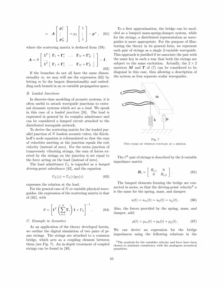
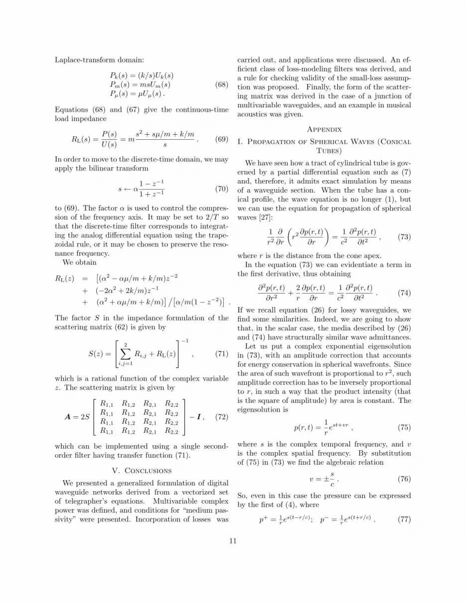