Multiple stages classification of Alzheimer's disease based on structural brain networks using...
10
Multiple stages classification of Alzheimers disease based on structural brain networks using Generalized Low Rank Approximations (GLRAM) Zhan L, Nie Z, Ye J, Wang Y, Jin Y, Jahanshad N, Prasad G, de Zubicaray GI, McMahon KL, Martin NG, Wright MJ, Thompson PM Abstract To classify each stage for a progressing disease such as Alzheimers dis- ease is a key issue for the disease prevention and treatment. In this study, we derived structural brain networks from diffusion-weighted MRI using whole-brain tractog- raphy since there is growing interest in relating connectivity measures to clinical, cognitive, and genetic data. Relatively little work has used machine learning to make inferences about variations in brain networks in the progression of the Alzheimers disease. Here we developed a framework to utilize generalized low rank approxima- tions of matrices (GLRAM) and modified linear discrimination analysis for unsu- pervised feature learning and classification of connectivity matrices. We apply the methods to brain networks derived from DWI scans of 41 people with Alzheimers disease, 73 people with EMCI, 38 people with LMCI, 47 elderly healthy controls and 221 young healthy controls. Our results show that this new framework can sig- nificantly improve classification accuracy when combining multiple datasets; this suggests the value of using data beyond the classification task at hand to model variations in brain connectivity. Zhan, Jin, Jahanshad,Prasad and Thompson Imaging Genetics Center, Department of Neurology, Keck School of Medicine, University of Southern California, Los Angeles, CA 90089, USA, e-mail: [email protected] Nie, Ye and Wang School of Computing, Informatics, and Decision Systems Engineering, Arizona State University, Tempe, AZ, USA de Zubicaray and McMahon fMRI Laboratory, University of Queensland, Brisbane, Australia Martin and Wright Berghofer Queensland Institute of Medical Research, Australia The final publication will be available at http://link.springer.com/book/10.1007/978-3-319-11182- 7. Computational Diffusion MRI. MICCAI Workshop, Boston, USA, September 18, 2014.. L. O’Donnell, G.Nedjati-Gilani,, Y. Rathi, M. Reisert, and T. Schneider. (Eds.), Springer-Verlag 2015. 1
Transcript of Multiple stages classification of Alzheimer's disease based on structural brain networks using...

Multiple stages classification of Alzheimersdisease based on structural brain networks usingGeneralized Low Rank Approximations(GLRAM)
Zhan L, Nie Z, Ye J, Wang Y, Jin Y, Jahanshad N, Prasad G, de Zubicaray GI,
McMahon KL, Martin NG, Wright MJ, Thompson PM
Abstract To classify each stage for a progressing disease such as Alzheimers dis-
ease is a key issue for the disease prevention and treatment. In this study, we derived
structural brain networks from diffusion-weighted MRI using whole-brain tractog-
raphy since there is growing interest in relating connectivity measures to clinical,
cognitive, and genetic data. Relatively little work has used machine learning to make
inferences about variations in brain networks in the progression of the Alzheimers
disease. Here we developed a framework to utilize generalized low rank approxima-
tions of matrices (GLRAM) and modified linear discrimination analysis for unsu-
pervised feature learning and classification of connectivity matrices. We apply the
methods to brain networks derived from DWI scans of 41 people with Alzheimers
disease, 73 people with EMCI, 38 people with LMCI, 47 elderly healthy controls
and 221 young healthy controls. Our results show that this new framework can sig-
nificantly improve classification accuracy when combining multiple datasets; this
suggests the value of using data beyond the classification task at hand to model
variations in brain connectivity.
Zhan, Jin, Jahanshad,Prasad and Thompson
Imaging Genetics Center, Department of Neurology, Keck School of Medicine, University of
Southern California, Los Angeles, CA 90089, USA, e-mail: [email protected]
Nie, Ye and Wang
School of Computing, Informatics, and Decision Systems Engineering, Arizona State University,
Tempe, AZ, USA
de Zubicaray and McMahon
fMRI Laboratory, University of Queensland, Brisbane, Australia
Martin and Wright
Berghofer Queensland Institute of Medical Research, Australia
The final publication will be available at http://link.springer.com/book/10.1007/978-3-319-11182-
7. Computational Diffusion MRI. MICCAI Workshop, Boston, USA, September 18, 2014.. L.
O’Donnell, G.Nedjati-Gilani,, Y. Rathi, M. Reisert, and T. Schneider. (Eds.), Springer-Verlag
2015.
1

2 Zhan et al. Multi-stage classification using GLARM
1 Introduction
Alzheimer’s disease is by far the leading form of dementia. There is no cure for the
disease, which worsens as it progresses, and eventually leads to death. According to
the studies of Alzheimers Disease Neuroimaging Initiative (ADNI) and other large-
scale multicenter studies, this disease has been described into four stages: health
control (HC); early mild cognitive impairment (EMCI), late mild cognitive impair-
ment (LMCI) and Alzheimers disease (AD)[1, 2, 3]. HC means there is no sign/clue
that subject have any cognition impairment, while EMCI and LMCI are the mid-
dle stages in time for disease detection. AD is the last stage when there is clearly
clue that disease has been onset. Defining atrisk stages of this disease is crucial for
predementia detection, which in turn is the requirement for future predementia treat-
ment. In literature, the Alzheimers disease multiple stages classification is mainly
based on subjective questionnaire[1, 4]. Here we adopted machine learning method
to explore multiple stages automatic classification using diffusion-weighted MRI
(DW-MRI).
DW-MRI is a non-invasive brain imaging technique, sensitive to aspects of the
brains white matter microstructure that are not typically detectable with standard
anatomical MRI.[5] With DWI, anisotropic water diffusion can be tracked along
the direction of axons using tractography methods. When tractography is applied to
the entire brain, one can reconstruct major fiber bundles and describe connectivity
patterns in the brains anatomical network [6]. Brain networks and topological mea-
sures derived from them have been shown to be highly associated with aspects of
brain function and clinical measures of disease burden [7]. Some studies have begun
to apply machine learning techniques to identify network features that differentiate
people with various neurological and psychiatric disorders from matched HC [8].
However, most studies focus only on identifying abnormal connectivity patterns in
a single disease, compared to controls, and not intermediate stages of the disease,
using only using one dataset to do so. While this may improve our understanding of
the outcome of the disease, when applying the same analysis to a new disease or a
new dataset, the model must be re-trained and re-evaluated. Often, disease effects (or
effects of other predictors on brain networks) are subtle and may not be detected in
one dataset alone, or may show conflicting results across datasets. In this light, con-
sortia such as Enhancing Neuro Imaging Genetics through Meta-Analysis (Enigma)
have been formed to jointly analyze over 20,000 brain scans from patients and con-
trols scanned at over 100 sites worldwide to meta-analyze effects on the brain [9].
This allows researchers to compare effect sizes obtained with different imaging pro-
tocols and scanners, but also across different diseases. The notion of who qualifies as
a healthy control may also depend on the dataset and may not represent the healthy
population at large. If multiple datasets are used to model normal variation, then
arguably diagnostic classification may be improved without retraining new models
for every disease and every new dataset.
When pooling scans from patients with a variety of diseases, or at different stages
of disease progression, machine learning techniques can classify the data into diag-
nostic groups. This may involve feature extraction, dimension reduction, model

Zhan et al., Multi-stage classification using GLARM 3
training and testing. For example, Principal Component Analysis (PCA) uses an
orthogonal linear transformation to convert observations of potentially correlated
variables into a new set of linearly uncorrelated principal components (PC). New
datasets can then be classified into groups based on PC-projected features. Linear
discriminant analysis (LDA) can also be used for dimensionality reduction and clas-
sification. It finds a linear combination of features that optimally separates two or
more classes. LDA and PCA both use linear combinations of variables to model the
data. LDA models the differences between classes within the data, but PCA seeks
components that have the highest variance possible under the constraint that they
are orthogonal to (i.e., uncorrelated with) the preceding components [10]. These
dimensionality reduction methods assume that the data form a vector space. Here,
each subjects data is modeled as a vector and the collection of subjects is modeled
as a single data matrix. Each column of the data matrix corresponds to one subject
and each row corresponds to a feature. There are disadvantages of this vector model,
as it overlooks spatial relations within the data. To overcome this, Generalized Low
Rank Approximations of Matrices (GLRAM) has been proposed to use a lower di-
mension 2D matrix to obtain more compact representations of original data with
limited loss of information [11].
In this study, we combined two different datasets collected with both standard
T1-weighted MRI and DW-MRI and created connectivity networks for all study
partici-pants. Both datasets had scanned healthy controls; one had also scanned pa-
tients with Alzheimers disease and patients with early and advanced signs of mild
cognitive impairment (early MCI and late MCI respectively). We merged this data
hypothesizing that we could automatically classify the scans into four groups (HC,
EMCI, LMCI, and AD) using brain networks as the raw features. We used GLRAM
to first reduce the dimensionality, and then applied LDA in the PCA subspace to
classify the data. Classification of data from multiple sites and scanners will help us
to understand differences in disease progression, ideally unconfounded by scanner
differences.
2 Subjects and Methods
2.1 Data Description
Table 1 summarizes the two datasets used in this study. For all datasets, participants
were scanned with both DW-MRI and standard T1-weighted structural MRI.
The first dataset included 221 healthy young adults. Images were acquired with
a 4T Bruker Medspec MRI scanner, using single-shot echo planar imaging with the
following parameters: TR/TE = 6090/91.7ms, 23cm FOV, and a 128x128 acquisi-
tion matrix. Each 3D volume consisted of 55 2-mm axial slices, with no gap, and
1.79x1.79mm2 in-plane resolution. 105 image volumes were acquired per subject:

4 Zhan et al. Multi-stage classification using GLARM
11 with T2-weighted b0 volumes and 94 diffusion-weighted volumes (b = 1159
s/mm2).
The second dataset was from ADNI2, the second stage of the Alzheimers Disease
Neuroimaging Initiative (ADNI), publically available online (http://adni.loni.usc.edu).
This dataset has 199 subjects, which includes 47 healthy elderly controls, 111 with
mild cognitive impairment (MCI) and 41 with Alzheimers disease (AD). Images
were acquired with 3T GE Medical Systems scanners at 14 sites across North Amer-
ica. Each 3D volume consisted of 2.7mm isotropic voxels with a 128x128 acquisi-
tion matrix. 46 image volumes were acquired per subject: 5 T2-weighted b0 images
and 41 diffusion-weighted volumes (b = 1000 s/mm2).
Table 1: Summary of data used in this study
Dataset 1 Dataset 2
Type Number Age Sex Number Age Sex
HC 221 24.1±2.1 85M 47 72.6±6.2 21M
EMCI
N/A
73 72.3±7.9 44M
LMCI 38 72.6±5.6 24M
AD 41 75.5±9.0 25M
2.2 Proposed framework
First, we first used GLRAM to create dimensionality-reduced matrices for each
sub-ject. These new matrices were used as input to LDA on PCA for model train-
ing. Adaptive 1-nearest neighbor classification (A-1NNC) was used to label the test
cases. The frameworks flowchart is shown in Fig. 1.
2.2.1 Brain Network Computation
In this study, we used the subjects structural networks as features for classification.
To compute the brain networks, FreeSurfer (http://freesurfer.net/) was run on the T1-
weighted images to automatically segment the cortex into 68 unique regions (34 per
hemisphere). This segmentation was dilated with an isotropic box kernel of 5mm to
ensure cortical labels would intersect with the white matter tissue in areas of reliable
tractography for the connectivity analysis. We registered the T1-weighted intensity
image to the fractional anisotropy (FA) image from the DWI data. The resultant
transformations were used to transform the dilated cortical segmentations into the
DWI space.
DWI images were corrected for eddy current distortions using FSL [12]. Then we
used an optimized global probabilistic tractography method [13] to generate whole
brain tractography for each subject. We combined the cortical segmentation and

Zhan et al., Multi-stage classification using GLARM 5
tractography to compute a connectivity matrix for each subject. The matrices were
68 x 68 in dimension, corresponding to the 68 segmented cortical regions. Each cell
value of the matrix represented the number of fibers that intersected pairs of cortical
regions. We normalized the matrix by the total number of fibers per subject. This
symmetric 68x68 matrix served as the input for our classification.
2.2.2 Data Normalization
Some form for data normalization is critical especially when working with data
from different cohorts or projects, covering a wide age range. So directly pooling
two datasets may introduce bias, if the proportion of controls depends on the scan-
ner used or scanning site. To account for these confounds, we used generalized
linear regression to adjust each value in the brain connectivity matrix for age, sex
and scanning site. Then we further normalized the residual after regression to yield
centered, scaled data, which served as the input for next step. This normalization
used a Z-transformation based on the standardized statistic Z=(X-mean(X))/std(X),
where X is one feature vector within each dataset. For our connectivity matrix, X is
element(i,j) for all subjects in each dataset.
Fig. 1: Flowchart of proposed framework for connectivity based disease classification.

6 Zhan et al. Multi-stage classification using GLARM
2.2.3 GLRAM
The purpose of GLRAM, proposed in [11], is similar to singular value decomposi-
tion (SVD) but has lower computational cost; it finds a lower rank 2D matrix Di to
approximate the original 2D matrix Ai, realizing the following function:
minL,R,D
N
∑i=1
∥
∥Ai −LDiRT∥
∥
2
F(1)
Here, Ai is each subjects raw brain network, N is the total number of subjects,
Di is the reduced representation of Ai; and L and R are transformation matrices on
the left and right side, respectively. F is the Frobenius norm. Details of how to solve
this cost function optimization problem are in [11].
2.2.4 LDA on the PCA subspace
PCA finds linear projections that maximize the scatter of all projected samples.
Mathematically, given a set of N subjects X = {x1,x2, ...xN}, where each subject
belongs to one of C classes X1, X2, , XC, we plan to map xi to yi where yi ∈ Rm and
m¡n. To do this, we define a linear transformation W to satisfy yi=WT xi (i=1,2,N).
In PCA, the optimal projection Wopt−pca is defined as:
Wopt−pca = argmaxw
∣
∣W T STW∣
∣
ST =N
∑i=1
(xi −µ)(xi −µ)T (2)
Here µ ∈Rn is the mean value of all samples. And Wopt−pca = {wi ∈ Rn |i = 1..m}is the set of eigenvectors of ST corresponding to the m largest eigenvalues. Once
eigenvectors are determined, all data can be projected into this eigenspace for clas-
sification. However, PCA is not optimal for classification as the dimensions that
model the greatest amount of variance in the data are not typically the ones that best
differentiate groups. In other words, the discriminant dimensions could be thrown
out or intermixed during PCA.
LDA seeks a projection to maximize the ratio of the determinant of the between-
class scatter matrix (SB) of the projected data to the determinant of the within-class
scatter matrix (SW ) of the projected data. However, the within-class scatter matrix
SW in LDA is typically singular. This is because the number of subjects is often
much smaller than the number of variables in the data. To overcome the complica-
tion of a singular SW , we adopted the solution in [14]. In short, C is the number
of classes, so we first adopted PCA to reduce the dimension of the feature space to
N-C , and then we applied the standard LDA to reduce the dimension to C-1, so the
transformation Wopt is given by:
Zhan et al., Multi-stage classification using GLARM 7
Wopt =Wopt−pcaWopt−pca−lda
Wopt−pca−lda = argmaxw|W T W T
opt−pcaSBWopt−pcaW ||W T W T
opt−pcaSW Wopt−pcaW |
SB =C
∑i=1
Ni(µi −µ)(µi −µ)T
Sw =C
∑i=1
∑xk∈Xi
(xk −µi)(xk −µi)T
(3)
Where i is the mean vector of class Xi, and Ni is the number of samples in class
Xi. Also, Wopt−pca can be computed using Eq. 2.
2.2.5 Adaptive 1-NNC
We classified the subjects class membership based on the Euclidean distance using
1-nearest neighbor classification (1-NNC). 1-NNC is designed to assign an object
to the same class as its single nearest neighbor. Adaptive 1-NNC (A-1NNC) is a
varia-tion of 1-NNC. The test objects class membership is still decided based on the
class membership of the single nearest-neighbor used for training, but once a new
test objects class membership has been determined, it is grouped into training group
to enhance the membership class affinity.
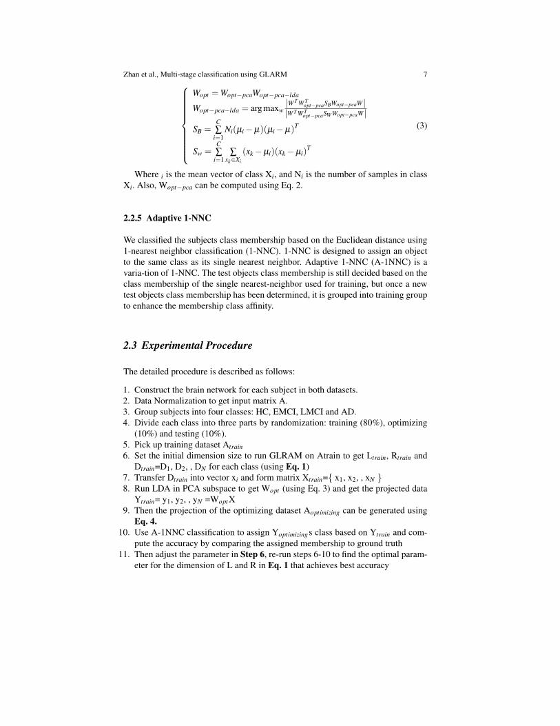
2.3 Experimental Procedure
The detailed procedure is described as follows:
1. Construct the brain network for each subject in both datasets.
2. Data Normalization to get input matrix A.
3. Group subjects into four classes: HC, EMCI, LMCI and AD.
4. Divide each class into three parts by randomization: training (80%), optimizing
(10%) and testing (10%).
5. Pick up training dataset Atrain
6. Set the initial dimension size to run GLRAM on Atrain to get Ltrain, Rtrain and
Dtrain=D1, D2, , DN for each class (using Eq. 1)
7. Transfer Dtrain into vector xi and form matrix Xtrain={ x1, x2, , xN }8. Run LDA in PCA subspace to get Wopt (using Eq. 3) and get the projected data
Ytrain= y1, y2, , yN =WoptX
9. Then the projection of the optimizing dataset Aoptimizing can be generated using
Eq. 4.
10. Use A-1NNC classification to assign Yoptimizings class based on Ytrain and com-
pute the accuracy by comparing the assigned membership to ground truth
11. Then adjust the parameter in Step 6, re-run steps 6-10 to find the optimal param-
eter for the dimension of L and R in Eq. 1 that achieves best accuracy

8 Zhan et al. Multi-stage classification using GLARM
12. Use this optimal parameter achieved in Step 11, and use the test dataset to test
our framework and get final grade
13. Repeat steps 4-12 (100 times) and compute the area under the curve (AUC) for
overall classification accuracy, as well as for the accuracy of each class. The
higher the AUC, the better the model performance.
Doptimizing
= LTtrainAoptimizingRtrain
Doptimizing
→ Xoptimizing
Yoptimizing
=WoptXoptimizing
(4)
3 Results and Discussion
Before we ran classification experiments, we first studied the effects of pooling
datasets 1 and 2 together. A testable null hypothesis is that the feature set in the
dataset 1 and dataset 2 are independent random samples drawn from Normal distri-
butions with equal means and equal but unknown variances. As each subjects brain
network is symmetric and has dimension 68x68, we have 68x67/2=2278 features
per subject. Thus we adopted False Discovery Rate (FDR) to account for the mul-
tiple comparisons (FDR q=0.05). Figure 2 shows the FDR-corrected P map from
a Students t-test between dataset 1 (all HC) and HC from dataset 2. Our results
showed that by using our proposed normalization methods, there are no detectable
differences between the HCs in dataset 1 and dataset 2. Given this information, we
pooled data bettering an effort to boost statistical power.
Then we compared our proposed method with the other 3 methods including:
direct PCA, LDA in the PCA subspace, and GLRAM only. Table 2 shows the AUC
comparison for the 4-class (HC, EMCI, LMCI and AD) classification results using
dataset 2 only and then also using both datasets for defining the PCs. The results
indicated that our proposed framework performed better than other methods. As
shown in Table 2, PCA showed the poorest performance, which is reasonable as
PCA emphasizes the data variance, which is not necessarily useful for classifica-
tion. Also, GLRAM performed better than LDA. The possible explanation could be
that our features were the full brain networks, which emphasized the connections
between the nodes. So there may be some 2D spatial information in the features that
are ignored in the vector space model (LDA). Moreover, HC classification accuracy
improved when adding dataset 1, suggesting the advantage of pooling data, so long
as appropriate normalization is applied.
4 Conclusion
Here we presented a novel framework using GLRAM and modified LDA to reduce
the dimension of a 68x68 element structural brain connectivity network. We then
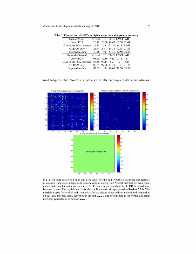
Zhan et al., Multi-stage classification using GLARM 9
Table 2: Comparison of AUCs. A higher value indicates greater accuracy
Dataset2 Only Overall HC EMCI LMCI AD
Direct PCA 26.19 26.50 46.47 17.50 22.44
LDA in the PCA subspace 26.31 59 21.20 9.25 13.67
GLRAM only 26.74 53.1 14.38 12.38 21.22
Proposed method 40.48 40 53.33 37.50 22.22
Dataset1+Dataset2 Overall HC EMCI LMCI AD
Direct PCA 65.43 82.36 5.25 5.75 14
LDA in the PCA subspace 66.48 90.14 5.2 2 5.11
GLRAM only 80.69 99.96 43.40 15 21.33
Proposed method 83.62 100 46.67 37.50 33.33
used Adaptive-1NNC to classify patients with different stages of Alzheimers disease
Fig. 2: An FDR-corrected P map (on a log scale) for the null hypothesis asserting that features
in datasets 1 and 2 are independent random samples drawn from Normal distributions with equal
means and equal but unknown variances. All P values larger than the critical FDR threshold have
been set to zero. The top left map is for the raw brain networks (generated in Section 2.2.1). The
top right map is for residual brain networks after the effects of age and sex are removed (regression
on age, sex and data label, described in section 2.2.2). The bottom map is for normalized brain
networks generated as in Section 2.2.2.

10 Zhan et al. Multi-stage classification using GLARM
versus healthy controls. Our proposed method outperformed classical classification
methods, but incorporating healthy controls from additional datasets also improved
classification.
As our proposed framework is based on some elementary approaches (such as
PCA and LDA), we compared these methods to ours, instead of other more com-
plex approaches. In future work, we will try more sophisticated approaches. As an
innovation, most current studies focus on one type disease vs. HC, while our tar-
get is for a more complicated (realistic) situation and we know there are ways to
improve the proposed framework. Our current results indicate that our approach is
promising.
References
1. Jessen F, Wolfsgruber S, Wiese B et al (2014) AD dementia risk in late MCI, in early MCI,
and in subjective memory impairment. Alzheimers Dement. 10:76–83.
2. Mitchell, AJ (2009) CSF phosphorylated tau in the diagnosis and prognosis of mild cogni-
tive impairment and Alzheimer’s disease: a meta-analysis of 51 studies. J Neurol Neurosurg
Psychiatry 80:966–975.
3. Aisen PS, Petersen RC, Donohue MC et al (2010) Clinical Core of the Alzheimer’s Disease
Neuroimaging Initiative: progress and plans. Alzheimers Dement 6:239–246.
4. Winblad B, Palmer K, Kivipelto M et al (2004) Mild cognitive impairment–beyond contro-
versies, towards a consensus: report of the International Working Group on Mild Cognitive
Impairment. J Intern Med 256:240–246.
5. LeBihan, D (1990) IVIM method measures diffusion and perfusion. Diagn Imaging (San
Franc) 12:133–136.
6. Sporns, O (2011) The human connectome: a complex network. Ann N Y Acad Sci 1224:109–
125.
7. Ajilore, O, Lamar M, Leow A et al (2014) Graph Theory Analysis of Cortical-Subcortical
Networks in Late-Life Depression. Am J Geriatr Psychiatry. 22:195–206.
8. Zhang, J., Cheng W., Wang Z et al(2012) Pattern classification of large-scale functional
brain networks: identification of informative neuroimaging markers for epilepsy. PLoS One
7:e36733.
9. Thompson, PM., Stein JL, Medland SE et al (2014) The ENIGMA Consortium: large-scale
collaborative analyses of neuroimaging and genetic data. Brain Imaging Behav 8:153–162.
10. Wang, J., Zhou L(2011) Research on magnetoencephalography-brain computer interface
based on the PCA and LDA data reduction. Sheng Wu Yi Xue Gong Cheng Xue Za Zhi
28:1069–1074.
11. Ye, J. (2005) Generalized Low Rank Approximations of Matrices. Mach. Learn. 61:167–191.
12. Jenkinson M, Beckmann CF, Behrens TE et al.(2012) FSL. Neuroimage 62:782–790
13. Aganj, I, Lenglet C, Jahanshad N et al (2011) A Hough transform global probabilistic ap-
proach to multiple-subject diffusion MRI tractography. Med Image Anal 15:414–425
14. Belhumeur PN, Hespanha JP, Kriegman DJ (1997) Eigenfaces vs. fisherfaces: Recognition
using class specific linear projection. Pattern Analysis and Machine Intelligence, IEEE Trans-
actions on 19:711–720.