1

Two-Dimensional Modeling and Analysis ofGeneralized Random Mobility Models for

Wireless Ad Hoc NetworksDenizhan N. Alparslan and Khosrow Sohraby,Senior Member, IEEE

Abstract— Most important characteristics of wireless ad hocnetworks such as link distance distribution, connectivity, andnetwork capacity are dependent on the long-run properties ofthe mobility profiles of communicating terminals. Therefore, theanalysis of the mobility models proposed for these networksbecomes crucial. The contribution of this paper is to providean analytical framework that is generalized enough to performthe analysis of realistic random movement models over two-dimensional regions. The synthetic scenarios that can be cap-tured include hotspots where mobiles accumulate with higherprobability and spend more time, and take into considerationlocation and displacement dependent speed distributions. Bythe utilization of the framework to random waypoint mobilitymodel, we derive an approximation to the spatial distribution ofterminals over rectangular regions. We validate the accuracyof this approximation via simulation, and by comparing themarginals with proven results for one-dimensional regions wefind out that the quality of the approximation is insensitive tothe proportion between dimensions of the terrain.

Index Terms— Mobility Modeling, Long-Run Analysis, Ad HocNetworks, Two-Dimensional Regions.

I. I NTRODUCTION

IN WIRELESS ad hoc networks communicating termi-nals move with respect to many different mobility

patterns each one having unique attributes. Therefore, mobilitymodeling and its analysis become very important for theperformance evaluation of these kinds of networks. In thispaper, we focus on the long-run location and speed distributionanalysis of a generalized random mobility modeling approachover two-dimensional mobility terrains.

The modeling methodology we are concentrating on isoriginally defined in [1] as a generalized model that is flexibleenough to capture the major characteristics of several realisticmovement profiles. In that paper, long-run location and speeddistributions are given in closed form expressions for one-dimensional regions. Here, we extend the analysis to two-dimensional terrains. A variety of examples are also givento show how the proposed model and its long-run analysisframework work for a broad range of mobility modelingapproaches.

In what follows, we give a brief description of the gen-eralized random mobility characterization approach that isanalyzed in this article. LetR denote the two-dimensional

(c)20xx IEEE. Personal use of this material is permitted. However, permis-sion to reprint/republish this material for advertising or promotional purposesor for creating new collective works for resale or redistribution to servers orlists, or to reuse any copyrighted component of this work in other works, mustbe obtained from the IEEE.

D. N. Alparslan is with The MathWorks, Inc., MA, USAK. Sohraby is with School of Computing and Engineering, University of

Missouri - Kansas City, MO, USA

bounded region on which mobile terminals operate. A mobilelocated at the pointXs = (Xs1

,Xs2) ∈ R, selects a random

point Xd = (Xd1,Xd2

) ∈ R as destination according to theconditional probability density function (pdf)fXd|Xs

(xd|xs),and moves to pointXd on the straight line segment joiningthe two points, and at a speedV that is drawn randomlyfrom the interval[vmin, vmax], wherevmin > 0, according tothe conditional pdffV |Xs,Xd

. After reaching the destination,mobile pauses for a random amount of time, denoted byTp,atXd, which is distributed with respect to the conditional pdffTp|Xd

, and whole cycle is repeated by selecting a new desti-nation. Hence, the pattern of a mobile terminal is composed ofconsecutive movement epochs between the randomly selectedpointsXs andXd, and it is uncorrelated with the movementbehaviors of other terminals. Throughout this paper, we usethe triplet< fXd|Xs

, fV |Xs,Xd, fTp|Xd

> to characterize themovement pattern of a mobile that moves with respect to thismodel.

Among the parameters of the triplet< fXd|Xs, fV |Xs,Xd

,fTp|Xd

>, the conditional pdffXd|Xsidentifies the distribution

of Xd given Xs at the embedded points in time wherea new movement epoch starts. Incorporation of this kernelinto this mobility characterization methodology providestheability to define hotspots on the two-dimensional mobilityterrain where mobiles accumulate with higher probability,and correlations between consecutive hotspot decisions canbe successfully modeled. Furthermore, sinceV is randomlydrawn fromfV |Xs,Xd

, we have the flexibility of constructinga correlation between the distribution ofV and the locationsof the starting pointXs and destinationXd. For instance, ascenario that identifiesV proportional to the distance that isgoing to be traveled, that is,|Xs −Xd|, can be easily defined.In addition, the usage offTp|Xd

makes it possible to capturedifferent pause distributions at different destinations availablefor the mobility model.

For wireless ad hoc networks, there have been proposed anumber of different mobility models. Comprehensive surveysof these models can be found in [2], [3]. Among them, therandom waypoint model [4] is one of the most widely usedone for analytic and simulation-based performance analysis ofad hoc networks. In this model, a mobile selects a destinationpoint in the mobility terrain with equal probability, and movesto that point with a speed that is drawn uniformly from agiven range. After reaching the destination, mobile pausesfor arandom time, which has a distribution that is independent fromthe current location, and whole cycle is repeated by selectinga new destination. In [5], [6], [7], analytical frameworks arepresented for the long-run analysis of this mobility model.

2

The analysis that we propose in this paper is also applicableto random waypoint model, and to demonstrate the correctnessand superiority of our work, we present a comparison of theresults derived with the ones presented in literature.

The rest of this paper is outlined as follows. In Section II,we describe analytical framework we developed for long-runanalysis. Section III provides the long-run distributionsfor alimited version of the exact mobility formulation constructedaccording to the methodology explained in the second section.Section IV utilizes the results reached in section three toderive approximations for the long-run distributions of thegeneralized model proposed. In Section V, we focus onexample scenarios, and the final section presents a summaryof the paper.

II. M ETHODOLOGY AND DESCRIPTION OFANALYTICAL

FRAMEWORK

In this section, we describe the analytical framework weestablish for the long-run analysis of the generalized mobilitymodel proposed.

Now since the movement behavior of mobiles are assumedto be uncorrelated with each other, we can concentrate on asingle terminal for long-run analysis. Hence, for the termi-nal whose movement pattern is characterized by the triplet< fXd|Xs

, fV |Xs,Xd, fTp|Xd

>, let the vectorX(t) denotethe state descriptor whose components identify the currentlocation, destination, and the speed of that mobile at timet. Inour solution methodology, we discretisize the two-dimensionalmobility terrain R and approximate the random variableVwith a discrete random variable so that the stochastic process{X(t), t ≥ 0} can be defined on a multidimensional discretestate space. The assumptions that we have made to generatethis discrete state space are as follows:

A1: The bounded regionR is discretisized inton disjoint,non-overlapping cells of the same shape denoted byci,i = 0 . . . n− 1, such thatR ⊆

⋃n−1i=0 ci wheren > 1. A

mobile terminal is assumed to occupy one of theci’sat any moment in time, and movement epochs occurbetween two randomly picked starting and destinationcells.

A2: The random variableV , that is, the speed during amovement epoch, is approximated by the discrete ran-dom variableV ∗ defined on the state spaceSV ∗ ={z1, z2, . . . , zm} where zr = r∆v, r = 1, . . . ,m, forsome discretization parameter∆v > 0, and an integerm ≥ 1 such that∆v ≤ vmin andvmax = m∆v.

Based on these assumptions, observe that a mobile can be inpausing or moving modes at the cell it is currently located.

Additionally, instead of observing the state of a terminalcontinuously, we observe it at embedded times denoted byTk, for k ∈ N, such thatT0 = 0, Tk+1 ≥ Tk, ∀k ∈ Z

+,which point to the time of occurrence of one of the followingevents:

E1: The terminal which is in pause mode, selects a new cell asdestination that is different from the current cell occupied,and changes its state to moving state in the current cellit is located,

1,11,0 1,2 1,3 1,4 1,6

0,10,0 0,2 0,4 0,5 0,6

2,0 2,2 2,3 2,4

3,13,0 3,2 3,3 3,4 3,5 3,6

4,14,0 4,2 4,3 4,4 4,5 4,6

5,15,0 5,2 5,4 5,5 5,6

6,0

0,3

6,1 6,2 6,3 6,4 6,5 6,6

1,5

2,5

2,1

5,3

line 0

line 1

line 2

line 3

line 4

line 5

line 6

(1/2)(1/2)

2,6γ2

γ3

γ1

γ0

Fig. 1. Discretization of the square regionR into squares.

E2: The terminal which is traveling in the direction of thetarget cell, moves out from the current cell and enters theneighboring cell that lies on the shortest path between thecurrent and destination cells,

E3: The terminal reaches to the destination cell and enters thepause mode at that location.

In our analysis, to apply assumptionA1, which is done toapproximate the exact location that can be occupied by a termi-nal at any point in time, we focus on the discretization methodsthat partition the regionR into squares or hexagons. Thereasoning behind concentrating on two different discretizationapproaches forR concurrently will become more clear as weproceed further in the long-run analysis. In Fig. 1, we applythesquare discretization approach to a square region. Visualizationof a discretization that is performed by hexagons can be foundin [8].

In Fig. 1, we also depict the scheme we decide on to identifythe cells on the discretisized region. Basically, the centers ofthe cells are grouped by lines that are parallel to each other,and the indexi of cell ci is denoted byi = (ℓi, ℓ

′i) whereℓi

represents the line that the center ofci is located, andℓ′i is itslocation on that line. For the rest of this paper, we will usethe notationsci and c(ℓi,ℓ′i)

interchangeably. Hence, if therearenℓ lines, and ifqℓ denotes the number of cells on lineℓ,then set of the cells on the discretisized region can be definedas follows:

R =

nℓ−1⋃

ℓ=0

{c(ℓ,0), . . . , c(ℓ,qℓ−1)}, (1)

Clearly, the path traveled during a movement epoch de-scribed by the discretisized version of the mobility charac-terization we constructed is composed of consecutive straightline segments between the centers of the cellsci, i =0, . . . , n− 1. In other words, a mobile terminal moves to oneof the neighboring cells from the current cell occupied whiletraveling towards the destination cell. Hence, ifd denotes thenumber of available movement directions for the discretisizedmobility formulation, thend would be equal to the numberof the sides of the regular polygons used in the discretizationprocess. Thus,d = 4 for square discretization, andd = 6 forhexagonal discretization, and letγı, ı = 0, . . . , d − 1 denotethose directions (see cellc(2,5) in Fig. 1). On the other hand,in principle, if there are no obstacles on the regionR that canrestrict the movement directions, then mobile should be ableto move at any direction. Therefore, by discretizing the region,

3

we are also forced todiscretisize the movement direction.Obviously, if R is discretisized by regular polygons of thesame shape, as we are doing, thend can be at most equal tosix. Furthermore, if the discretization of a regionR with ageneral shape (e.g. rectangle) with regular polygons is donefor the purpose approximating the exact location of a terminal,as in our case, then using hexagons is a better choice becausethe number of available movement directions are higher, andamore realistic approximation can be done to the exact mobilitypattern.

At this point, it should be noted that, the enforcement ofdiscretizing movement directions will not arise for the one-dimensional case because there are only two directions for amobile to move on a one-dimensional region and discretizationmethod does not enforce any kind of restriction on thesedirections. Clearly the fundamental difference between thediscretization parametersd, and n and m is that n and mcan be increased, butd, as we have mentioned above, can beat most equal to six. This difference introduces a new issuethat has to be clarified before continuing. In what follows, weexplain this issue and our solution approach for it.

Now recall that according to our mobility model proposed,during a movement epoch, mobile travels on the straight linejoining the pointsXs and Xd. In the discretisized versionof this mobility model, movement epochs occur betweenrandomly selected cells. Obviously if the mobile terminal isallowed to move at any direction in the regionR, then theshortest path between those two points is just the straightline between them, and it is unique. However, for the discreteformulation, the shortest path is defined in terms of the numberof jumps between cells. More importantly, for a discretizationthat is done according to squares (i.e.,d = 4), or to hexagons(i.e., d = 6), if p(d)(i, j), d = 4, 6, denotes the ordered list ofthe cells that are located on a shortest path for the movementepoch that had started atci, and ended up at destination cellcj , then the members ofp(d)(i, j) will not be necessarilyunique. The algorithm that we use in this paper to generatep(d)(i, j) is as follows. If cj is towards the directionγı′ forsomeı′ ∈ {0, . . . , d − 1} from ci, then mobile follows thatdirection until it reaches destinationcj . On the other hand,mobile proceeds to the next cell either in the directionγı′ orγı′+1mod d with equal probabilities for someı′ ∈ {0, . . . , d−1}that generates the least possible shortest path if selected, andcontinues in that direction until it reaches to a cell that can bejoined tocj by following one of thed available directions. Forexample, in Fig. 1, consider the scenario whereci = c(2,1) andcj = c(5,3). Observe that for this scenario, this algorithm eithergenerates the path{c(2,1), c(2,2), c(2,3), c(3,3), c(4,3), c(5,3)} orthe path{c(2,1), c(3,1), c(4,1), c(5,1), c(5,2), c(5,3)}. It should bealso noted that, according to our notation, the first and the lastmembers of the listp(d)(i, j) areci andcj , respectively.

Having clarified these issues, we now proceed to the formaldefinition of the discretisized mobility formulation. DenoteSk,k ∈ N, as the state of the mobile terminal at timeTk. Hence,based on assumptionsA1, A2, and the eventsE1, E2, E3 thatidentify observation timesTk, for k ∈ N, the finite state-spaceof Sk will be defined as follows:

S = SM ∪ SP (2)

whereSM = {(ci, cj , zr, q) | i, j = 0, . . . , n− 1, i 6= j,

r = 1, . . . ,m, q = 1} (3)

SP = {(ci, q) | i = 0, . . . , n− 1, q = 0} (4)

whereci is the current cell occupied,cj is the destination cell,zr is the discretisized speed, andq is the indicator functionthat is defined as follows:

q =

{

1, mobile is moving towards the target cell0, mobile is pausing at the destination cell

(5)

Consequently, the stochastic process{X(t), t ≥ 0} can beformally defined on the finite-state spaceS according to thefollowing expression:

X(t) = Sk, if Tk ≤ t < Tk+1

Notice that whenX(t) occupies a states ∈ SM, since the states has a separate dimension for the destination cell, the nextstate to be visited can be determined from the components ofit. In other words, the future evolution of the stochastic process{Sk, k ∈ N} becomes dependent only on the current state ofthe mobile terminal, not on its history at previous observationpoints. Furthermore, for alls ∈ S, the distribution of sojourntime in states would be independent from the previous statesoccupied and can be determined only from the components ofstates.

Therefore, the stochastic process{Sk, Tk; k ∈ N} withfinite-state spaceS satisfies the conditions for beingMarkovRenewal Process, and the process{X(t), t ≥ 0} can becalled as thesemi-Markov process (SMP) associated with{Sk, Tk; k ∈ N} [9]. Moreover, since the distributions fordestination, speed, and pause time parameters are assumedto be time-homogeneous in the mobility model proposed, thedistribution of state holding time in states, given that thenext state to be visited iss′, would be independent ofk.Hence, the transitions of the processX(t) at the embeddedtime instantsTk can be governed by thediscrete-time Markovchain (DTMC) {Sk, k ∈ N} with finite-state spaceS in (2)and transition probability matrixP = [ps s′ ], whereps s′ =Pr{Sk+1 = s′ |Sk = s}, such that

∑

s′∈S ps s′ = 1 for alls ∈ S. The process{Sk, k ∈ N} is also referred asembeddedDTMC of SMP.

Thus, in order to characterize the SMP{X(t), t ≥ 0} at thelong-run, the DTMC{Sk, k ∈ N} must satisfy the ergodicityconditions and the mean state holding times must be finite.If these conditions are satisfied, then the long-run proportionof time spent in a states ∈ S can be obtained, and afteraggregating the states that has the samecurrent cell andspeedcomponents, the long-run distributions sought can be derivedfor this discretisized version of the mobility formulation.

Notice that, as the discretization parametersn → ∞ andm → ∞, we obtain better approximations to the locationand speed of the mobile terminals, respectively, and in thelimit we converge to a restricted version the continuous modelwhere the available movement directions are limited by theddifferent directionsγ0, . . . , γd−1 given by

γı =

{ 2π ıd , if d = 4,

2π (ı+1/2)d , if d = 6,

(6)

4

for ı = 0, . . . , d − 1. Visualization of these directions arealso provided in Fig. 1 ford = 4. Clearly because of themethodology we decided to generatep(d)(i, j), at the limitn→ ∞, the path followed during a movement epoch betweenXs andXd ∈ R will generally be composed of two directedfinite line segments towards the directionsγı1 andγı2 where{ı1 = ı, ı2 = (ı+1)mod d} or {ı1 = (ı+1)mod d, ı2 = ı} forsomeı ∈ {0, . . . , d− 1}. This can be also observed from theexample movement scenarios depicted in Fig. 1. Obviously ifXd is towards any of directionsγı, ı = 0, . . . , d − 1, fromXs, then the path will be composed of a single straight line.For the rest of this report we will use the termcontinuous-d mobility formulation to refer to this limited version of theexact continuous mobility formulation. Finally, we note that,sinced can be at most equal to six, a formal transition fromthis limited case to the original continuous formulation cannotbe done. Therefore, in the following sections we will usedistributions of the continuous-d mobility formulation to gainsome insight into the methodology that can be used to deriveapproximations for the long-run distributions of originalcase.

III. A NALYTICAL RESULTS FORTHE DISCRETISIZED AND

CONTINUOUS-d MOBILITY FORMULATION

In this section, we first concentrate on generating the long-run location and speed distributions for the discretisizedcase,and after that we will use those results to derive long-rundistributions of the continuous-d mobility formulation.

Now, to able to identify the transition probabilities of theDTMC {Sk, k ∈ N}, we first denoteτj|i as the probability ofselecting cellcj as target from cellci. Then, according to themobility characterization parameterfXd|Xs

, τj|i will be givenby

τj|i =

∫

xd∈cj

fXd|Xs(xd|Xs ∈ ci) dxd, (7)

Similarly, denoteνr|i,j as the conditional probability massfunction of V ∗ for a movement epoch that had started at cellci with destinationcj . Then, by using the parameterfV |Xs,Xd

we have

νr|i,j =

∫ r∆v

(r−1)∆v

fV |Xs,Xd(v|Xs ∈ ci,Xd ∈ cj) dv (8)

for r = 1, . . . ,m. In addition, letnh(ci) denote the cells in theneighborhood of cellci that can be reached in one jump fromit, and let[i′, i, j] denote the index of the cellci′ in the orderedlist that defines the pathp(d)(i, j). Note that,[i, i, j] = 1, and[j, i, j] =

∣

∣

∣

∣p(d)(i, j)∣

∣

∣

∣ where∣

∣

∣

∣p(d)(i, j)∣

∣

∣

∣ denotes the numberof the cells on the pathp(d)(i, j). Hence, if we are interestedin the probability of the cellci′ to be the next cell to be visitedafter cell ci, that is,Pr{[i′, i, j] = 2}, thenPr{[i′, i, j] = 2}is either equal to1, or 1/2, or 0 (i.e. ci′ is not on the pathp(d)(i, j)). For instance, in Fig. 1, whenci = c(2,1), cj =c(5,3), andci′ = c(2,2), thenPr{[i′, i, j] = 2} = 1/2. On theother hand, ifci = c(2,1), cj = c(2,3), and ci′ = c(2,2), thenPr{[i′, i, j] = 2} = 1.

Based on these definitions, the transition probabilities cor-responding to the eventsE1, E2, andE3, can be grouped asin Table I.

Next, we examine the irreducibility and aperiodicity of theDTMC {Sk, k ∈ N} with respect to the transition probabilitiesdefined in Table I. Letϕi denote the probability of starting a

TABLE I

TRANSITION PROBABILITIES OF THE PROCESS{Sk, k ∈ N}

Event Transition Probability Condition∗

E1 (ci, 0) → (ci, cj , zr, 1)τj|i

1−τi|iνr|i,j i 6= j

E2 (ci, cj , zr, 1) → (ci′ , cj , zr, 1) 1 cj /∈ nh(ci),Pr{[i′,i,j]=2} =

1

1/2 cj /∈ nh(ci),Pr{[i′,i,j]=2} =

1/2

E3 (ci, cj , zr, 1) → (cj , 0) 1 cj ∈ nh(ci)∗ i, i′, j = 0, . . . , n − 1, r = 1 . . . m

movement epoch from a cellci, i = 0, . . . , n−1 at the steady-state. Obviously, in order to satisfy the irreducibility,ϕi mustbe greater than0 for all i = 0, . . . , n − 1. Otherwise, somecells on the two-dimensional discretisized region will neverbe visited (i.e., selected as destination) and the chain becomesreducible. Hence, a steady-state distribution must exist forXs. The conditional pdffXd|Xs

(xd|xs), which identifies thedistribution ofXd givenXs at the embedded points in timewhere a new epoch starts, is referred asstochastic densitykernel by Feller [10]. Under some “mild” regularity conditionsdefined in [10] onfXd|Xs

(xd|xs) the steady-state distributionof Xs with pdf fXs

(xd) can be uniquely determined from thesolution of the following integral equation

fXs(xd) =

∫

xs∈R

fXd|Xs(xd|xs)fXs

(xs)dxs, (9)

andϕi will then be equal to

ϕi =

∫

xd∈ci

fXs(xd) dxd (10)

Observe that, ifT = [τj|i], and if the integral equation (9) hasa unique solution, thenϕi can be also obtained by solvingϕT = ϕ, ||ϕ||1 = 1 whereϕ = [ϕ0, . . . , ϕn−1].

In view of the discussions above, the following can be easilyproven.

Lemma 1: If the pdf fXs(xd) can be uniquely determined

from the solution of the integral equation (9), and ifνr|i,j > 0,i, j = 0, . . . , n − 1 and r = 1, . . . ,m, then the embeddedDTMC {Sk, k ∈ N} defined on state spaceS in (2), withtransition probabilities given as in Table I, is irreducible andaperiodic.

Next, we provide the steady-state distribution of the DTMC{Sk, k ∈ N}.

Lemma 2: For the DTMC{Sk, k ∈ N} defined on the statespaceS in (2), whered is either equal four or six, letπ(d)

i

and π(d)(i,j,r) denote the steady-state probabilities of being in

the states of the forms = (ci, 0), i = 0, . . . , n − 1, ands = (ci, cj , zr, 1), i, j = 0, . . . , n − 1, i 6= j, r = 1, . . . ,m,respectively. If the conditions of Lemma 1 are satisfied, thenthey are uniquely given by

π(d)i = ϕi (1 − τi|i)/N, (11)

π(d)i,j =

∑

ci′∈p(d)t,1 (i,j)

ϕi′ τj|i′ νm|i′,j/N

+ 12

∑

ci′∈p(d)t,2 (i,j)

ϕi′ τj|i′ νm|i′,j/N (12)

where

5

π(d)i,j = [π

(d)(i,j,1), . . . , π

(d)(i,j,m)], (13)

νm|i′,j = [ν1|i′,j , . . . , νm|i′,j ], (14)

andp(d)t,1 (i, j) =

{

ci′ |ci′ ∈ R,Pr{ci ∈ p(d)(i′, j)} = 1}

, (15)

p(d)t,2 (i, j) =

{

ci′ |ci′ ∈ R,Pr{ci ∈ p(d)(i′, j)} = 1/2}

,(16)

andN =∑n−1

i=0 π(d)i +

∑n−1i=0

∑n−1j=0,j 6=i

∣

∣

∣

∣

∣

∣π

(d)i,j

∣

∣

∣

∣

∣

∣

1.

Proof: Refer to [8].It should be noted that, the setsp(d)

t,1 (i, j) in (15) and

p(d)t,2 (i, j) in (16) represent the subset of cells inR from where

a movement epoch originated with destination cellcj passesthrough the cellci with probabilities 1 and 1/2, respectively.

Now, let ts denote the sojourn time of the SMP{X(t), t ≥0} in states ∈ S. Then, if s = (ci, cj , zr, 1) (i.e., mobile ismoving towards the destination with discrete speedzr), andif ∆c(d) denotes the traveled distance in a cell while passingtrough it, then

ts =∆c(d)

zr(17)

On the other hand, ifs = (ci, 0), then we define the following.

ts = E[Tpi] = E[Tp|Xs ∈ ci] (18)

Finally, in order to characterize the SMP{X(t), t ≥ 0} at thelong-run, the following must be satisfied [9]:

∑

s∈S

πsts <∞ (19)

Hence, by applying the theory of semi-Markov processeswe obtained the long-run proportion of time that the SMP{X(t), t ≥ 0} is in a states ∈ S. After aggregating the statesin S that has the samecurrent location andspeed components,including the ones with zero speed (i.e,s = (ci, 0)), we reachto the following result.

Lemma 3: For the mobile terminal, whose mobility patternis characterized according to the discretisized version ofthe< fXd|Xs

, fV |Xs,Xd, fTp|Xd

> mobility formulation, letp(d)i ,

i = 0, . . . , n− 1, d = 4, 6, denote the long-run proportion oftime that terminal stays in cellci, which can be a square orhexagon. Similarly, denoteψ(d)

r as the long-run proportion oftime that mobile possesses speedzr = rδv, r = 0, . . . ,m. Ifthe conditions given by Lemma 1 are satisfied, and equation(19) holds to be true, then

p(d)i =

ϕi (1 − τi|i)E[Tpi] +

m∑

r=1k

(d)i,r

N(d)n,m

, (20)

and

ψ(d)r =

n−1∑

i=0

ϕi (1 − τi|i)E[Tpi] /N

(d)n,m , if r = 0

n−1∑

i=0

k(d)i,r /N

(d)n,m , else

(21)

where

k(d)i,r =

∑

cj∈R−{ci}

(

∑

ci′∈p(d)t,1 (i,j)

ϕi′τj|i′1

zrνr|i′,j ∆c(d)

+ 12

∑

ci′∈p(d)t,2 (i,j)

ϕi′τj|i′1

zrνr|i′,j ∆c(d)

)

, (22)

c1

c3c2

c0

a0 a2

(a) n = 4, d = 4

c0 c1 c2 c3

a0 a2

c4 c5 c6 c7

c8 c9 c10 c11

c12 c13 c14 c15

(b) n = 16, d = 4

Fig. 2. Discretisized version of a simple mobility scenario.

andN (d)

n,m =

n−1∑

i=0

ϕi (1 − τi|i)E[Tpi] + D(d)

n (23)

whereD(d)

n =

n−1∑

i=0

m∑

r=1

k(d)i,r (24)

To simplify the formulation ofD(d)n in (24) for some special

cases, we now state the following claim.Claim 1: If the distribution ofV ∗ is assumed to be inde-

pendent from the location of the starting and destination cellsof the movement epochs, the expression forD

(d)n in (24) is

equivalent to the following:

D(d)n = E[

1

V ∗]∑

ci∈R

∑

cj∈R

ϕi τj|i dis(d)(i, j) ∆c(d), (25)

wheredis(d)(i, j) =∣

∣

∣

∣p(d)(i, j)∣

∣

∣

∣ − 1, that is, the number ofthe discrete jumps made on the pathp(d)(i, j).

Proof: Refer to [8].Before continuing on with the long-run analysis of the

continuous-d mobility formulation, in order to clarify theinterpretation of termk(d)

i,r given in (22), we now concentrateon a simple example scenario. Now, consider a continuousmobility formulation (i.e., mobiles can move anywhere at anydirection) over the regionR = [0, a] × [0, a] where V isdeterministic and equalv, and the other mobility character-ization parameters,fXd|Xs

and fTp|Xd, can be arbitrary as

long as the integral equation in (9) is uniquely solvable andequation (19) is satisfied. Now to be able to apply Lemma 3,we need to generate the discretisized version of this mobilityformulation. Hence, assumen = 4, d = 4, and sinceV isdeterministic,m = 1. In Fig. 2.(a) we provided a visualizationof the discretisized mobility model generated according tothese assumptions.

Now for this discretisized mobility formulation, if we areinterested in the long-run proportion of time mobile stays incell c0 (i.e.,p(4)

0 ), then according to Lemma 3 we simply have

p(4)0 =

ϕ0 (1 − τ0|0)E[Tp0] + k

(4)0,1

N(4)4,1

, (26)

where

k(4)0,1 =

a

2v(ϕ0τ1|0 + 1

2ϕ2τ1|2 + ϕ0τ2|0 + 12ϕ1τ2|1

ϕ0τ3|0 + ϕ1τ0|1 + ϕ2τ0|2 + ϕ3τ0|3), (27)

which is equal to the average time spent over the cellc0 whilemoving between randomly picked cells. In other words,k

(4)0,1

is equal toa/2v multiplied with the probability of a movement

6

epoch between two randomly picked cells that pass troughthe cell c0, including the ones starting or ending at cellc0.Notice that in this simple formulationνr|i′,j = 1 for alli′, j = 0, . . . , 3. However, if the distribution ofV is dependentonXs andXd in the original continuous mobility formulation,thenm > 1, and we have to multiply each additive term ofk

(4)0,r , r = 1, . . . ,m with the probability of selecting speedzr = rδv, (i.e.,νr|i′,j) and 1

zrfor the the movement epoch that

passes trough cellc0, as it is shown by the formulation ofk(d)i,r

in (22). Observe that, for all choices ofV , the term∑m

r=1 k(d)i,r

corresponds to the expected time spent over cellci whilemoving between two randomly picked cells that are drawnfrom the distributionsϕi′ in (10) andτj|i′ in (7), respectively.

Next we proceed to the long-run analysis of the continuous-d mobility formulation. At first, recall that in this case sincemovement directions are restricted to four or six differentdirections, the path followed during a movement epoch be-tween the pointsXs ∈ R and Xd ∈ R will be composedtwo or one line segments each directed towards one of theavailable directionsγı in (6), ı = 0, . . . , d− 1. Thus, in orderto keep the formulation of this case separate from the exactmodel, where movement epochs occur on a single directed linesegment that can have any direction, let the random variablesX(d)(t) = (X

(d)1 (t),X

(d)2 (t)) and V (d)(t), whered is either

four or six, denote the location and the speed of a mobileterminal at timet, respectively. Note thatX(d)(t) ∈ R, andsince the mobile can be in moving or pausing modes at anypoint in time, V (d)(t) is either equal to0, or in the range[vmin, vmax].

Now let X(d) = (X(d)1 ,X

(d)2 ) and V (d) denote the random

variables having the long-run distribution ofX(d)(t) andV (d)(t), respectively. Recall that in the discretisized versionof the mobility formulation, we assumed the random variablesX(d)(t) and V (d)(t) to take only discrete values, and inLemma 3, provided the long-run proportion of times that amobile stays in cellci, (i.e., p(d)

i in (20)), and possessesspeedzr (i.e., ψ(d)

r in (21)). Therefore, in order to derivethe distributions ofX(d) and V (d), we need to focus on thelimiting behavior of the discrete distributions given by Lemma3 as discretization parametersn andm approaches infinity.

As an illustration of the methodology that is going to beapplied during this transition, lets concentrate on the simplemobility formulation whose discretisized version is depictedin Fig. 2.(a). Recall that, in that simple modelV = v(i.e., deterministic) and the other mobility characterizationparameters can be arbitrary. Now for the discretisized case,let P (d)

n (a2 ) denote the long-run proportion of time mobile is

located in the regionR(a2 ) = [0, a

2 ] × [0, a2 ]. Hence, ifd = 4

andn = 4, we haveP

(4)4 (a

2 ) = p(4)0 (28)

wherep(4)0 is defined by (26). Notice that in this formulation

the discretization parameterm is skipped because sinceV =v, andm = 1.

Next, the important question is what will be the limitingform of P (4)

n (a2 ) in (28) asn → ∞. Hence, if we assume

n = 16, then discretisized region given in Fig. 2.(a) will betransformed to form given in Fig. 2.(b). By applying Lemma

3 we have

P(4)16 (a

2 ) =

∑

ci∈R( a2 )

ϕi (1 − τi|i)E[Tpi] +

∑

ci∈R( a2 )

k(4)i,1

N(4)16,1

, (29)

whereR(a2 ) = {c0, c1, c4, c5}, that is, the set of discrete cells

located on the regionR(a2 ).

Now based on the interpretation ofk(d)i,r in (22), the term

∑

ci∈R( a2 ) k

(4)i,1 corresponds to the average time spent over

R(a2 ) while moving between randomly picked two cells.

Notice that both of those cells or one of them can be alsobelong toR(a

2 ). Hence we reach to the following:

∑

ci∈R( a2 )

k(4)i,1 =

∑

cj∈R

∑

ci′∈R

ϕi′ τj|i′ P( a2 )(i

′, j)1

vJ( a

2 )(i′, j)∆c(d)

(30)where P( a

2 )(i′, j) denotes the probability passing over the

region R(a2 ) while moving from ci′ to cj , and J( a

2 )(i′, j)

represents the number of discrete jumps overR(a2 ) while mov-

ing. Notice that the termJ( a2 )(i

′, j)∆c(d) represents the totaldistance traveled overR(a

2 ), which is required to calculate theaverage time spent.

Therefore, in order to obtain the limiting form ofP (4)n (a

2 )as n → ∞, we need to derive the limiting expression ofthe double summation given in (30) which requires a properformulation ofP( a

2 )(i′, j) andJ( a

2 )(i′, j).

Thus, we now focus on the formalization of the observationswe mentioned above. In order to keep our formulation assimple as possible, we concentrate on deriving the long-rundistributions of the continuous-4 (i.e., d = 4) and continuous-6 (i.e., d = 6) mobility formulations over square and hexag-onal mobility terrains of side lengtha, respectively. Denotethese terrains with the generic notationR(d)(a), whered issubstituted by 4 if it is a square, else by 6 (i.e., hexagon).Also, to describe long-run location distribution consistentlywith d and the shape of mobility terrain (i.e.,R(d)(a)), wefocus on defining the probability mass function (pmf) ofX(d)

over a square subregion inR(4)(a), and a hexagonal subregionin R(6)(a). Let R(d)(x, b) denote these subregions, which isa square ifd = 4, and a hexagon ifd = 6, with centerx ∈ R(d)(a) and side lengthb such thatR(d)(x, b) ⊆ R(d)(a).In Fig. 3, we provided illustrations ofR(4)(a) andR(4)(x, b).We also denote byS(d)(a, b) the set of all nonintersectingR(d)(x, b) ⊆ R(d)(a).

In addition to the these notations, letL(d)(p, xs, xd, x, b)denote the length of the total distance traveled over thesubregionR(d)(x, b) for a movement epoch that occurs be-tween the pointsxs and xd, and passes throughR(d)(x, b)with probability p, which can be equal to1, 1/2, or 0 forthe continuous-d mobility formulation. In Fig. 3, we depictL(4)(p, xs, xd, x, b) for example movement epochs. Finally, wedefine

S(d)(p, xd, x, b)

= {xs|xs ∈ R(d)(a), L(d)(p, xs, xd, x, b) 6= 0} (31)Based on the notations given in the preceding two para-

graphs, we are now ready to state the main theorem of thissection.

7

x

b

ba

xs

xd

L(4)(12, xs, xd, x, b)

R(4)(x, b)xs xd

L(4)(1, xs, xd, x, b)

Fig. 3. Illustrations ofR(4)(a), R(4)(x, b), andL(4)(p, xs, xd, x, b).

Theorem 1: For the mobile terminal, whose mobility pat-tern is characterized by the continuous-d mobility formulationover the mobility terrainR(d)(a), d = 4, 6, let FX(d)(x, a, b)denote probability mass function ofX(d) over the subregionR(d)(x, b) ⊆ R(d)(a). Also, let fV (d) denote the pdf ofV (d).

If the pdf fXs(xd) can be uniquely determined from the in-

tegral equation (9), andE[Tp|Xs = xs] <∞, ∀xs ∈ R(d)(a),and fV |Xs,Xd

> 0, ∀ v ∈ [vmin, vmax], and ∀xs, xd ∈R(d)(a), then

FX(d)(x, a, b)

=

E[Tp|Xs∈R(d)(x,b)] Pr{Xs∈R(d)(x,b)} +vmax∫

vmin

K(d)(x,v,b,a) dv

E[Tp|Xs∈R(d)(a)]+D(d), (32)

and

fV (d)(v)=

E[Tp|Xs∈R(d)(a)]δ(v)

E[Tp|Xs∈R(d)(a)]+D(d), v = 0

P

R(d)(x,b)∈S(d)(a,b)

K(d)(x,v,b,a)

E[Tp|Xs∈R(d)(a)]+D(d), v ∈ [vmin, vmax]

(33)

where

K(d)(x, v, b, a)

=

∫

xd∈R(d)(a)

dxd

(

∫

xs∈S(d)(1,xd,x,b)

dxs k(d)(1,xs,xd,x,v,b)

+ 12

∫

xs∈S(d)(1/2,xd,x,b)

dxs k(d)(1/2,xs,xd,x,v,b))

, (34)

k(d)(p,xs,xd,x,v,b)

=fXs (xs)fXd|Xs(xd|xs) 1

vfV |Xs,Xd

(v|xs,xd)L(d)(p,xs,xd,x,b), (35)

and

D(d) =∑

R(d)(x,b)∈S(d)(a,b)

∫ vmax

vmin

dv K(d)(x,v,b,a) (36)

Proof: Refer to [8].We may note that the term

∫ vmax

vminK(d)(x,v,b,a) dv, where

K(d)(x, v, b, a) is given in (34), corresponds to the expectedtime spent over the regionR(d)(x, b) while moving betweenthe pointsXs andXd that are respectively drawn from thedistributions fXs

and fXd|Xs. Also, in order to formulate

L(d)(p, xs, xd, x, b) and the regionS(d)(p, xd, x, b) explicitly

we need to partitionR(d)(a) with respect toR(d)(x, b). Clearlythis will increase the complexity of the results presented byTheorem 1. However since we are aimed at using the distri-butions of the continuous-d case to reach some conclusionsabout the exact case, we decided to keep the presentation ofthe results given by Theorem 1 as simple as possible.

Now, in view of the result given by Claim 1 forD(d)n in

(25), if V (i.e., the speed for a movement epoch) is assumedto be independent from the distributions ofXs andXd, thenwe get the following forD(d) in (36):

D(d) = E[1

V]D(d) (37)

where

D(d) =

∫

xs∈R(d)(a)

dxs

∫

xd∈R(d)(a)

dxd fXs(xs)fXd|Xs

(xd|xs) |xs − xd|(d)

(38)where |xs − xd|

(d) represent the total distance traveled be-tween the pointsxs = (xs1

, xs2) andxd = (xd1

, xd2) for the

continuous-d mobility formulation. Clearly ifd = 4, then

|xs − xd|(4)

= |xd1− xs1

| + |xd2− xs2

| (39)

which is also know as theManhattan distance [11]. Also,notice that|xs − xd|

(4)> |xs − xd|

(6) , ∀xs, xd ∈ R.Finally, based on the definition ofD(d) in (38), theE[V (d)]

will be given by the following even if the distribution ofV isdependent on the distributions ofXs andXd.

E[V (d)] =D(d)

E[Tp|Xs ∈ R(d)(a)] + D(d)(40)

IV. CONTINUOUS MOBILITY FORMULATION

In this section, we concentrate on the long-run properties ofthe continuous mobility formulation. In order to be as genericas possible, the mobility terrainR is assumed to be rectangulardefined byR = [0, a1] × [0, a2]. DenoteX(t) and V (t),respectively, as the location and speed of a mobile terminalattime t. Because we are interested in the long-run distributions,let X and V respectively denote the random variables havingthe long-run distribution ofX(t) and V (t). Notice that thestate spaces ofX andX(d), andV andV (d) are the same butsince the continuous-d mobility formulation puts restrictionon the movement directions, their long-run speed and locationdistributions will be always different from each other.

Now as mentioned before, sinced can be either equal tofour or six, the results provided by Theorem 1 cannot beextended formally to cover the exact case that allows mobileto move at any direction. Therefore, we now concentrate onusing the results of Theorem 1 to construct an approximationmethodology for the long-run distributions of the originalcontinuous case.

Hence, analogous to the definition ofR(d)(x, b) insideR(d)(a) (see Fig. 3), we define the following rectangularsubregion insideR = [0, a1]× [0, a2] for the continuous case:

R(x,∆x1,∆x2) = [x1 −∆x1

2 , x1 + ∆x1

2 ]

× [x2 −∆x2

2 , x2 + ∆x2

2 ] (41)

8

xd

xs

x10 a1

0

a2

xx2

L(xs, xd, x, ∆x1, ∆x2)

∆x1

∆x

2

: The region S(xd, x, ∆x1, ∆x2)

Fig. 4. Illustrations ofS(xd, x, ∆x1, ∆x2) and L(xs, xd, x, ∆x1, ∆x2)for the continuous mobility formulation.

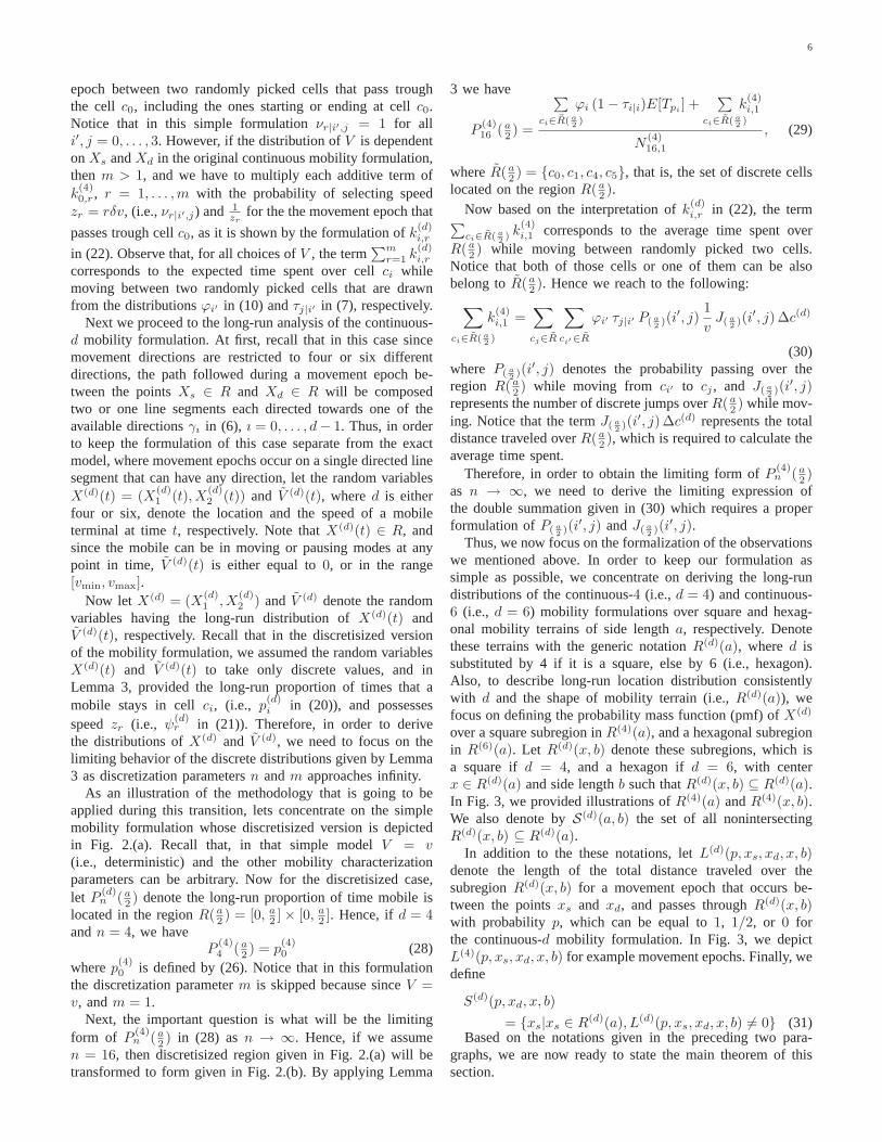
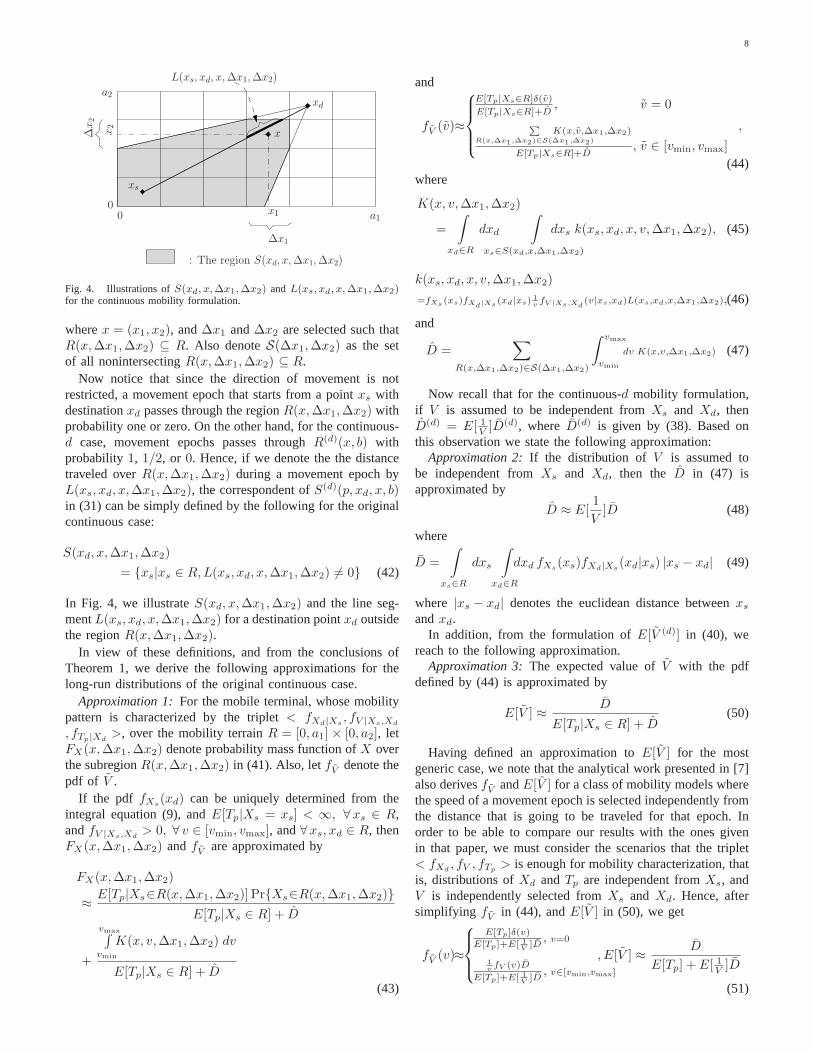
wherex = (x1, x2), and∆x1 and∆x2 are selected such thatR(x,∆x1,∆x2) ⊆ R. Also denoteS(∆x1,∆x2) as the setof all nonintersectingR(x,∆x1,∆x2) ⊆ R.

Now notice that since the direction of movement is notrestricted, a movement epoch that starts from a pointxs withdestinationxd passes through the regionR(x,∆x1,∆x2) withprobability one or zero. On the other hand, for the continuous-d case, movement epochs passes throughR(d)(x, b) withprobability 1, 1/2, or 0. Hence, if we denote the the distancetraveled overR(x,∆x1,∆x2) during a movement epoch byL(xs, xd, x,∆x1,∆x2), the correspondent ofS(d)(p, xd, x, b)in (31) can be simply defined by the following for the originalcontinuous case:

S(xd, x,∆x1,∆x2)

= {xs|xs ∈ R,L(xs, xd, x,∆x1,∆x2) 6= 0} (42)

In Fig. 4, we illustrateS(xd, x,∆x1,∆x2) and the line seg-mentL(xs, xd, x,∆x1,∆x2) for a destination pointxd outsidethe regionR(x,∆x1,∆x2).

In view of these definitions, and from the conclusions ofTheorem 1, we derive the following approximations for thelong-run distributions of the original continuous case.

Approximation 1: For the mobile terminal, whose mobilitypattern is characterized by the triplet< fXd|Xs

, fV |Xs,Xd

, fTp|Xd>, over the mobility terrainR = [0, a1] × [0, a2], let

FX(x,∆x1,∆x2) denote probability mass function ofX overthe subregionR(x,∆x1,∆x2) in (41). Also, letfV denote thepdf of V .

If the pdf fXs(xd) can be uniquely determined from the

integral equation (9), andE[Tp|Xs = xs] < ∞, ∀xs ∈ R,andfV |Xs,Xd

> 0, ∀ v ∈ [vmin, vmax], and∀xs, xd ∈ R, thenFX(x,∆x1,∆x2) andfV are approximated by

FX(x,∆x1,∆x2)

≈E[Tp|Xs∈R(x,∆x1,∆x2)] Pr{Xs∈R(x,∆x1,∆x2)}

E[Tp|Xs ∈ R] + D

+

vmax∫

vmin

K(x, v,∆x1,∆x2) dv

E[Tp|Xs ∈ R] + D

(43)

and

fV (v)≈

E[Tp|Xs∈R]δ(v)

E[Tp|Xs∈R]+D, v = 0

P

R(x,∆x1,∆x2)∈S(∆x1,∆x2)

K(x,v,∆x1,∆x2)

E[Tp|Xs∈R]+D, v ∈ [vmin, vmax]

,

(44)where

K(x, v,∆x1,∆x2)

=

∫

xd∈R

dxd

∫

xs∈S(xd,x,∆x1,∆x2)

dxs k(xs, xd, x, v,∆x1,∆x2), (45)

k(xs, xd, x, v,∆x1,∆x2)

=fXs (xs)fXd|Xs(xd|xs) 1

vfV |Xs,Xd

(v|xs,xd)L(xs,xd,x,∆x1,∆x2),(46)

and

D =∑

R(x,∆x1,∆x2)∈S(∆x1,∆x2)

∫ vmax

vmin

dv K(x,v,∆x1,∆x2) (47)

Now recall that for the continuous-d mobility formulation,if V is assumed to be independent fromXs and Xd, thenD(d) = E[ 1

V ]D(d), where D(d) is given by (38). Based onthis observation we state the following approximation:

Approximation 2: If the distribution of V is assumed tobe independent fromXs and Xd, then the D in (47) isapproximated by

D ≈ E[1

V]D (48)

where

D =

∫

xs∈R

dxs

∫

xd∈R

dxd fXs(xs)fXd|Xs

(xd|xs) |xs − xd| (49)

where |xs − xd| denotes the euclidean distance betweenxs

andxd.In addition, from the formulation ofE[V (d)] in (40), we

reach to the following approximation.Approximation 3: The expected value ofV with the pdf

defined by (44) is approximated by

E[V ] ≈D

E[Tp|Xs ∈ R] + D(50)

Having defined an approximation toE[V ] for the mostgeneric case, we note that the analytical work presented in [7]also derivesfV andE[V ] for a class of mobility models wherethe speed of a movement epoch is selected independently fromthe distance that is going to be traveled for that epoch. Inorder to be able to compare our results with the ones givenin that paper, we must consider the scenarios that the triplet< fXd

, fV , fTp> is enough for mobility characterization, that

is, distributions ofXd andTp are independent fromXs, andV is independently selected fromXs andXd. Hence, aftersimplifying fV in (44), andE[V ] in (50), we get

fV (v)≈

E[Tp]δ(v)

E[Tp]+E[ 1V

]D, v=0

1v

fV (v)D

E[Tp]+E[ 1V

]D, v∈[vmin,vmax]

, E[V ] ≈D

E[Tp] + E[ 1V ]D

(51)

9

whereδ(v) is defined as the direc delta function. The aboveformulation of fV and E[V ] are consistent with the onesgiven in [7]. Hence, our approximations forfV and E[V ]becomes exact for the mobility characterizations done by< fXd

, fV , fTp>.

We should also note that, the results presented by Approx-imations 1, 2, and 3, becomes exact for a mobility modelingthat restricts the available movement directions to 4 or 6different choices that are exactly defined byγı in equation(6). As an application of this case, consider a mobility scenariowhere mobiles are only allowed to move on the grids over themobility terrain.

We finally note that, since we can only prove the limiteddirection case, we can never state that these approximationsare highly accurate for all possible mobility scenarios definedby the triplet< fXd|Xs

, fV |Xs,Xd, fTp|Xd

>. Fundamentally,their accuracy is dependent on the frequency of the movementepochs that is targeted to a destination point with a movingdirection outside the directionsγı in (6), where ı = 4, 6.Hence, in Section V, we concentrate on the applicabilityand accuracy of our approximations for some example casesthat allows mobiles to move at any direction when travelingtowards the destination point. The methodology we follow inSection V to analyze the accuracy of the approximations canbe also applied to analyze other example mobility cases.

A. Approximation to the pdf of long-run location distribution

Before proceeding further, we now focus on simplifyingthe results of Approximation 1 to derive an approximationto the pdf of long-run location distribution in closed form.Hence, letfX denote the pdf ofX, that is, the random variablehaving the long-run distribution ofX(t). It then follows fromthe definition given in [12] for the pdf of bivariate randomvariables that

fX(x) = lim∆x1→0∆x2→0

FX(x,∆x1,∆x2)

∆x1 ∆x2(52)

At this point, the important question is, given the triplet< fXd|Xs

, fV |Xs,Xd, fTp|Xd

>, whether it is possible to finda closed form expression for the termK(x, v,∆x1,∆x2) in(45) so that the above limit can be taken explicitly. If thiscan be done, then we can state an approximation tofX(x) inclosed form.

To answer this question, we first concentrate on a simplescenario whereXd is uniformly distributed overR for a givenXs, and V is characterized byfV . Obviously for this case,K(x, v,∆x1,∆x2) in (45) simplifies to

K(x, v,∆x1,∆x2)

=fV (v)

(a1 a2)2 v

∫

xd∈R

dxd

∫

xs∈S(xd,x,∆x1,∆x2)

dxs L(xs, xd, x,∆x1,∆x2)(53)

Therefore, to be able to derive a closed form expressionfor K(x, v,∆x1,∆x2), the integrandL(xs, xd, x,∆x1,∆x2)must be expressible in terms of a function that can beanalytically integrated over the given integration region.

:S1(xd, x, ∆x1, ∆x2)

:S3(xd, x, ∆x1, ∆x2)

:S2(xd, x, ∆x1, ∆x2)

∆x1

x1

xd

0 a1

a2

0

∆x

2

x2

xs

xs

xs

Fig. 5. Partitioning the regionS(xd, x, ∆x1, ∆x2).

Now from the definition ofL(xs, xd, x,∆x1,∆x2), andalso from Fig. 4, observe that

L(xs, xd, x,∆x1,∆x2) = (g(xs, xd, x,∆x1,∆x2))1/2 (54)

for a function g(xs, xd, x,∆x1,∆x2) that is piecewise con-tinuous onS(xd, x,∆x1,∆x2) for given xd ∈ R. Clearly,the analytical integration ofL(xs, xd, x,∆x1,∆x2) in (54)over the given 4-dimensional integration region (see (53))is complicated. Hence, we conclude that obtaining a closedform expression forK(x, v,∆x1,∆x2) even for the simplestof all possible mobility characterization parameters is nearlyimpossible.

However, if some exceptional choices ofxs = (xs1, xs2

)and xd = (xd1

, xd2) are not taken into consideration, for

example, suppose thatxs, xd /∈ R(x,∆x1,∆x2), |xd1− x1|

> ∆x1

2 , and |xd2− x2| >

∆x2

2 , thenL(xs, xd, x,∆x1,∆x2)will be expressible in terms of an easily integrable functionfor some mobility characterization choices.

To be more precise, on the rectangular mobility terrainR = [0, a1] × [0, a2] assumexd1

> x1 + ∆x1

2 andxd2

> x2 + ∆x2

2 . Furthermore, letℓR(x1) denote the linesegment joining the pointsxd and (x1 + ∆x1

2 , x2 − ∆x2

2 ),and assumeℓR(0) > 0. In Fig. 5, we provided a visual-ization of these assumptions. Notice that this special casealso implies |xd1

− xs1| > |xd2

− xs2|. In addition, con-

sider the partitioning of the subregionS(xd, x,∆x1,∆x2)into three subregions as shown in Figure 5, and denoteLr(xs, xd, x,∆x1,∆x2), r = 1, 2, 3, as the distance traveledoverR(x,∆x1,∆x2) whenxs ∈ Sr(xd, x,∆x1,∆x2). Next,formulatingLr(xs, xd, x,∆x1,∆x2) explicitly we get

Lr(xs, xd, x,∆x1,∆x2)

=

|xd−xs|∆x1

xd1−xs1

, r=2

|xd−xs|(x2+cr

∆x22 −xs2

xd2−xs2

−x1+cr

∆x12 −xs1

xd1−xs1

), r=1,3

(55)

wherec1 = 1 andc3 = −1.Before we proceed further, it should be noted that, for

the formulation that assumesxd1> x1 + ∆x1

2 and xd2>

x2 + ∆x2

2 , if we had concentrated on the case that onlyallows |xd2

− xs2| > |xd1

− xs1|, and had partitioned

S(xd, x,∆x1,∆x2) in the same way as we did in Fig. 5, then

10

theLr(xs, xd, x,∆x1,∆x2), r = 1, 3, would be also definedby (55). However, ifr = 2, then

L2(xs, xd, x,∆x1,∆x2) =|xd−xs|∆x2

xd2−xs2

, (56)

which is expected intuitively.Now returning back to case that is constructed according

to the assumption|xd1− xs1

| > |xd2− xs2

|, it is clearthatL2(xs, xd, x,∆x1,∆x2) > Lr(xs, xd, x,∆x1,∆x2), r =1, 3 (also observe it from Fig. 5). Hence, concentrating onL2(xs, xd, x,∆x1,∆x2) observe the following:

L2(xs, xd, x,∆x1,∆x2) = ∆x1

s

1+(xd2

−xs2)2

(xd1−xs1

)2, (57)

Obviously as the difference between|xd1−xs1

| and|xd2−xs2

|

increases, the term(xd2

−xs2)2

(xd1−xs1

)2 converges to zero. Hence, wecan state the following:

L2(xs, xd, x,∆x1,∆x2) ≈ ∆x1 (58)

Finally, sinceL2(xs, xd, x,∆x1,∆x2) is always more dom-inant thanLr(xs, xd, x,∆x1,∆x2), r = 1, 3, we conclude thefollowing approximation.

L(xs, xd, x,∆x1,∆x2)≈

{

∆x1, |xd1−xs1

|>|xd2−xs2

|

∆x2, |xd1−xs1

|<|xd2−xs2

|(59)

As a result, if mobility model is simple enough to stateK(x, v,∆x1,∆x2) as in (53), and if the above substitutionfor L(xs, xd, x,∆x1,∆x2) is used, then the result of Approx-imation 1 can be simplified to derive an approximation forfX

in closed form after tedious symbolic integrations. We alsoconcentrate on the applicability of this statement in the nextsection.

V. EXAMPLE SCENARIOS

Example 1: The random waypoint model proposed in [4],which is commonly used to model node movement by theperformance analysis studies for wireless ad hoc networks,can be considered as the simplest nontrivial case for themobility characterizations that can be analyzed accordingtothe triplet < fXd|Xs

, fV |Xs,Xd, fTp|Xd

>. For this model,the distributions ofXd and V are assumed to be uniformin the regionsR and [vmin, vmax], respectively. Moreover,the distribution ofTp is considered to be the same at alldestinations. Therefore, for the rectangular mobility terrainR = [0, a1] × [0, a2], we simply have

fXs(xd) =

{

1a1 a2

, if xd ∈ [0, a1] × [0, a2]

0, otherwise(60)

Hence, form Approximations 1 and 2 we reach the followingapproximation for the pmf ofX overR(x,∆x1,∆x2) in (41):

FX(x,∆x1,∆x2)≈

E[Tp]∆x1 ∆x2

a1 a2+ E[ 1

V ]KX(x,∆x1,∆x2)

E[Tp] + E[ 1V ]D

(61)where

KX(x,∆x1,∆x2)

=

∫

xd∈R

dxd

∫

xs∈S(xd,x,∆x1,∆x2)

dxs L(xs, xd, x,∆x1,∆x2) (62)

xd

• • • • • sr1

x2

∆x

2

x1

∆x1

: The region S(xd, x, ∆x1, ∆x2)

Fig. 6.Partitioning ofS(xd, x, ∆x1, ∆x2) into sr subregions for a givenxd.

where E[ 1V ] =

ln( vmaxvmin

)

(vmax−vmin) , and D is given by (49). In

addition, fV andE[V ] can be derived respectively from theequations in (51).

In order to assess the accuracy of the approximationwe stated forFX(x,∆x1,∆x2) by equation (61) for therandom waypoint model, we will now focus on the taskof evaluatingFX(x,∆x1,∆x2) in (61) numerically for allR(x,∆x1,∆x2) ∈ S(∆x1,∆x2), and comparing them withthe results derived from the simulation of the random waypointmobility model.

Hence, observe first that to generate an approximation toFX(x,∆x1,∆x2) from (61) for a givenR(x,∆x1,∆x2), weneed to evaluateKX(x,∆x1,∆x2) numerically in (62), whichis defined by a 4-dimensional integral. Obviously, the accuracyof a result that can be derived from a numerical integrationmethodology is dependent on thesmoothness of the integrandover the integration region [13]. Therefore, to increase theaccuracy of our numerical experiments, we partition the regionS(xd, x,∆x1,∆x2) into sr subregions, wheresr ≥ 1, so thatthe integrandL(xs, xd, x,∆x1,∆x2) (see (62)) evaluated fora fixedxd deviates less for all of thexs that belongs to thosesubregions. In Fig. 6, we illustrated this partitioning method-ology for a givenxd. Next, to evaluate the 4-dimensionalintegrals for each of these subregions, we first transformedthem to an integral over a hypercube [13]. Then, each of theresulting integrals are evaluated by repeated one-dimensionalintegrations according to the Gauss’ Formula [14]. Clearly, thisis not “economical”, however, it is required in order to evaluatethe accuracy of our approximation. The program implementingthis methodology is designed in a generic form in order to alsocapture different mobility characterization parameters,and itis available from authors.

In order to assess the accuracy of the approximation toFX(x,∆x1,∆x2), a simple simulation model is developedconsisting of a single node moving according to the randomwaypoint mobility profile. In this model, during each sim-ulation run, the node travels forne number of movementepochs. For each movement epoch, the time spent at eachR(x,∆x1,∆x2) ∈ S(∆x1,∆x2), while passing through it orpausing at it, is exactly calculated, and added to the total timespent at the subregionR(x,∆x1,∆x2) for the whole simula-tion run. At the end of the run,FX(x,∆x1,∆x2) is derived bynormalizing the total time spent atR(x,∆x1,∆x2) to the total

11

0.316

0.226

0.183

0.254

0.212

0.425

0.632

0.688

0.491

0.563

0.385

0.226

0.127

0.133

0.223

0.352

0.346

0.221

0.171

0.143

0.194

0.4

0.353

0.259

0.25

0.167

0.216

0.355

0.205

0.2

0.246

0.259

0.323

0.291

0.159

0.215

0.241

1.291

0.501

0.468

0.256

0.345

0.709

0.41

0.494

1.2311.237

1.04

a1

a2

6

a2

6

a2

6

a2

6

a2

6

a2

a1

82a1

83a1

84a1

85a1

86a1

87a1

80

0

Percentage of Error: E(S,A)X (b(1), b(2)) × 100

(a)

2.427

0.839

0.329

0.301

0.865

2.476

2.434

0.802

0.406

0.326

0.844

2.436

1.752

0.328

0.323

0.33

0.331

1.72

1.659

0.348

0.395

0.442

0.295

1.691

0.201

0.551

0.11

0.180

0.536

0.092

0.048

0.483

0.142

0.182

0.566

0.172

4.07

1.432

0.189

0.388

1.503

3.862

3.805

1.353

0.377

0.47

1.573

3.868

a1

a2

6

a2

6

a2

6

a2

6

a2

6

a2

a1

82a1

83a1

84a1

85a1

86a1

87a1

80

0

Percentage of Error: E(S,A)X (b(1), b(2)) × 100

(b)

Fig. 7. E(S,A)X (b(1), b(2)) for Example 1 (a1 = 1200, a2 = 900, b

(1)1 = i a1/8, i = 0, . . . , 7, b

(1)2 = b

(1)1 + a1/8, b

(2)1 = j a2/6, j = 0, . . . , 5,

b(2)2 = b

(2)1 + a2/6, vmin = 1 m/s, vmax = 20 m/s, Tp = U [0, 30] sec).

run time of the experiment.nr independent replications of thisexperiment is run, and the finalFX(x,∆x1,∆x2) is obtainedby averaging the results of these runs. Also, at the beginningof each replication, the initial location, and speed and pausetime distributions of the node is determined according to themethodology explained in [6] for the efficient and reliablesimulation of random waypoint mobility model.

Now to be able to represent a comparison of the results ob-tained form (61), and from the simulation model we describedabove, consider the region[b(1)1 , b

(1)2 ]× [b

(2)1 , b

(2)2 ] ⊆ R where

b(1)i , i = 1, 2, and b(2)j , j = 1, 2, are multipliers of∆x1 and

∆x2, respectively. Notice that ifPX(b(1), b(2)) denotes theprobability of the mobile terminal to be located over the region[b

(1)1 , b

(1)2 ]× [b

(2)1 , b

(2)2 ] at the long-run, thenPX(b(1), b(2)) can

be easily derived by accumulating all of theFX(x,∆x1,∆x2)

such thatR(x,∆x1,∆x2) ⊂ [b(1)1 , b

(1)2 ] × [b

(2)1 , b

(2)2 ]. Hence,

let P (A)X (b(1), b(2)) and P

(S)X (b(1), b(2)) respectively denote

the correspondent ofPX(b(1), b(2)) obtained from (61) (i.e.,Approximation 1) and from the simulation model. Based onthese notations, we define the following metric to asses thecorrectness of our conjecture for this mobility model.

E(S,A)X (b(1), b(2)) =

|P(S)X (b(1), b(2)) − P

(A)X (b(1), b(2))|

P(S)X (b(1), b(2))

,

(63)Finally, for our experiments, we considered a[0, 1200]m

×[0, 900]m mobility terrain, and set the parameters of mobilityas follows:vmin = 1m/s, vmax = 20m/s, andTp is uniformover the range[0, 30]sec. Then, we chose∆x1 = ∆x2 = 5m,and setne = 107, nr = 100 for the simulation experiment,and evaluatedE(S,A)

X (b(1), b(2)) for various choices ofb(1)i

and b(2)i , i = 1, 2. The results are presented in Fig. 7.(a).Simulation results are acquired with a95% confidence in-terval lower than0.001. Since the percentage of error, (i.e.,E

(S,A)X (b(1), b(2)) × 100) is at most1.29% we conclude that

the application of the Approximation 1 to random waypointmobility model is accurate.

Thus, usingFX(x,∆x1,∆x2) in (61) we can obtain an

approximation to the pmf ofX = (X1,X2) over the sub-regionR(x,∆x1,∆x2) numerically. With this knowledge athand, we will now concentrate on findingE[X1], E[X2], andCorr(X1,X2). Hence, we set∆x1 = a1

n1and∆x2 = a2

n2for

some discretization parametersn1, n2 ∈ Z+, and define the

discrete bivariate random variableX∗ = (X∗1 ,X

∗2 ) with the

finite state space

S∗={∆x12 ,

3∆x12 ,...,

(2n1−1)∆x12 }×{∆x2

2 ,3∆x2

2 ,...,(2n2−1)∆x2

2 } (64)

to denote the subregionR(x∗,∆x1,∆x2) in (41), wherex∗ ∈S∗, that the mobile is located at the long-run. Clearly, asn1 →∞ and n2 → ∞, X∗ converges to the continuous bivariaterandom variableX.

Evaluating the distribution ofX∗ from FX(x,∆x1,∆x2)in (61) we obtainedE[X∗

1 ], E[X∗2 ], and Corr(X∗

1 ,X∗2 )

numerically for several different parameter choices for therandom waypoint mobility model. For all of the scenarioswe considered, we setn1 and n2 sufficiently large enoughto closely approximateX = (X1,X2) with X∗ = (X∗

1 ,X∗2 ),

and observed the following:

E[X∗1 ] =

a1

2, E[X∗

2 ] =a2

2, Corr(X∗

1 ,X∗2 ) = 0 (65)

The simulation studies presented in [15], [16] points out thatthe long-run location distribution of the random waypointmobility model is more accumulated at the center of themobility terrain. More importantly, it is symmetric with respectto center. Therefore, obtainingE[X∗

1 ] andE[X∗2 ] as in (65) is

expected. However, the result forCorr(X∗1 ,X

∗2 ) = 0 is not

observed before. In fact, our numerical experiments showedthatX∗

1 andX∗2 are not independent.

It should also be noted that analytical work presented in[5] for the spatial node distribution generated by this mobilitymodel concentrates on the case whereR = [0, a] × [0, a],V is deterministic with parameterv, and E[Tp] = 0, andformulates the long-run cumulative distribution functionovera region with an area ofδ2. If we substituteE[1/V ] with 1

v ,andE[Tp] = 0, and assume∆x1 = ∆x2 = δ, anda1 = a2,the formulation of the approximation we defined by (61) for

12

FX(x,∆x1,∆x2) becomes consistent with the formulation ofthe cumulative distribution function given in [5].

We now focus on applying the approximation we definedby (59) forL(xs, xd, x,∆x1,∆x2) to derive an approximationto fX(x) in (52) (i.e., the pdf ofX). First, notice fromthe formulation ofKX(x,∆x1,∆x2) in (62) that when thisapproximation is used, the integration of the integrand overthe regionS(xd, x,∆x1,∆x2), will be equal to∆x1 or ∆x2

times the area of the regionS(xd, x,∆x1,∆x2). Hence, bypartitioning the boundaries of the 4-dimensional integrationthat formulatesKX(x,∆x1,∆x2) according to the condition|xd1

−xs1| > |xd2

−xs2| and its counterpart appropriately, we

obtained a closed form expression for (62). Finally, evaluatingthe limit FX(x,∆x1,∆x2)

∆x1 ∆x2as ∆x1 → 0 and ∆x2 → 0, we

reached the following approximation forfX :

fX(x) ≈ fX(x) (66)

where

fX(x) =E[Tp]

1a1 a2

+ E[ 1V ]k(x)/N

E[Tp] + E[ 1V ]D

(67)

where

k(x)=

k1(x)+k4(x)+k6(x)+k8(x), 0<x1<a12 , 0<x2<

a2x1a1

k1(x)+k4(x)+k6(x)+k8(x), a12 <x1<a1, 0<x2<a2(1−

x1a1

)

k2(x)+k4(x)+k5(x)+k8(x), 0<x1<a12 ,

a2x1a1

<x2<a2(1−x1a1

)

k1(x)+k3(x)+k6(x)+k7(x), a12 <x1<a1, a2(1−

x1a1

)<x2<a2x1

a1

k2(x)+k3(x)+k5(x)+k7(x), 0<x1<a12 , a2(1−

x1a1

)<x2<a2

k2(x)+k3(x)+k5(x)+k7(x), a12 <x1<a1,

a2x1a1

<x2<a2

(68)wherex = (x1, x2), andki(x), i = 1, . . . , 8 are defined by

k1(x) = (a1−x1)x2[2 a2 x1+a1(x1−x2)+x1 x2g1(x)]

2 a21 a2

2 x1

k2(x) = x1(a2−x2)[2 a1 x2+a2(x2−x1)−x1 x2g1(x)]

2 a21 a2

2 x2

k3(x) = (a1−x1)(a2−x2)[a2(x1−a1)+x2(a2+2a1)+(a1−x1)x2g2(x)]

2 a21 a2

2 x2

k4(x) = x1 x2[(a1+2 a2)(a1−x1)−a1 x2−(a1−x1)x2g2(x)]

2 a21 a2

2(a1−x1)

k5(x) = x1(a2−x2)[a1(a1−x1+x2)+a2(a1−2x1)−(a1−x1)(a2−x2)g1(x)]

2 a21 a2

2(a1−x1)

k6(x) = (a1−x1)x2[a2(a1+a2+x1)−(2 a1+a2)x2+(a1−x1)(a2−x2)g1(x)]

2 a21 a2

2(a2−x2)

k7(x) = (a1−x1)(a2−x2)[2 a2 x1+a1(x1+x2−a2)+x1(a2−x2)g2(x)]

2 a21 a2

2 x1

k8(x) = x1 x2[a2(2 a1+a2−x1)−(2 a1+a2)x2−x1(a2−x2)g2(x)]

2 a21 a2

2(a2−x2)

where

g1(x)=log(x1(a2−x2)

(a1−x1)x2), g2(x)=log(

x1 x2(a1−x1)(a2−x2)

) (69)

and N is the normalization term given by

N =(

∫

x∈R

k(x) dx)

/D (70)

It should be noted that since the termL(xs, xd, x,∆x1,∆x2)is either substituted by∆x1 or ∆x2, the functionk(x) in (68)must be normalized in the regionR so thatfX(x) will be aprobability density function.

In order to asses the validity of the approximation wepresented by (66) we evaluatedP (A)

X (b(1), b(2)) by integratingfX(x) in (67) over the region[b(1)1 , b

(1)2 ] × [b

(2)1 , b

(2)2 ] and

compared the results with simulation. In Fig. 7.(b) we pro-vided theE(S,A)

X (b(1), b(2)) for the same mobility parameterchoices we considered in Fig. 7.(a). From the values ofE

(S,A)X (b(1), b(2)) for different [b(1)1 , b

(1)2 ]× [b

(2)1 , b

(2)2 ] ⊆ R, we

reached to the conclusion that the approximation we statedby (66) for the long-run spatial distribution of the randomwaypoint model over the given rectangular mobility terrainis quite accurate. Also notice that, the percentage of errors(i.e., E(S,A)

X (b(1), b(2)) × 100) presented in Fig. 7.(a). arebetter than the ones in Fig. 7.(b). This is expected becauseto evaluate theE(S,A)

X (b(1), b(2)) in Fig. 7.(a), we computedFX(x,∆x1,∆x2) directly from equation (43). However, inFig. 7.(b), we approximatedL(xs, xd, x,∆x1,∆x2) by equa-tion (59) to evaluateFX(x,∆x1,∆x2), which decreased thequality of the approximation but gave us an approximation tofX(x) in closed form.

In addition, if one is interested in a variant of random way-point mobility model where mobiles may pause at different atdifferentXd, that is,fTp|Xd

needs to be employed in mobilitycharacterization in stead offTp

, then the approximation givenin (67) can be redefined as follows:

fX(x) =E[Tp|Xd = x] 1

a1 a2+ E[ 1

V ]k(x)/N

E[Tp|Xd ∈ R] + E[ 1V ]D

(71)

where E[Tp|Xd = x] is the expected pause time at thedestination pointx, and

E[Tp|Xd] =

∫

xd∈R

dxdfXs(xd)E[Tp|Xd = xd] (72)

Finally, we note that in [5] authors also present a veryaccurate approximation for the pdf ofX for the special case ofthe original random waypoint model whereR = [0, 1]× [0, 1],and speed choice for all movement epochs is constant. In orderto compare that approximation with the one given in this papernumerically for this special case (i.e.,R = [0, 1] × [0, 1] andspeed is constant), we evaluated cumulative long-run locationdistributions for several subregions overR according to both ofthem. We observed for various choices ofE[Tp] andV that therelative error between the results obtained from approximationand simulation is at most2% for both of the approximationmethods defined in [5] and in (66).

Example 2: According to the results that are proved in[1] for the one-dimensional version of the random waypointmobility model, the probability distribution function ofX1

(i.e., the first component ofX = (X1,X2)) over the mobilityterrainR = [0, a1] is

FX1(x1) =

x1

a1E[Tp] +

x21(a1−2x1/3)

a21

E[ 1V ]

E[Tp] + a1

3 E[ 1V ]

(73)

Now, it is clear that an approximation to the marginaldistribution of X1 can be stated from the approximationdefined by (66) for the joint probability density function ofX = (X1,X2) as follows:

F(A)X1

(x1) =

∫ x1

0

du

∫ a2

0

dvfX(u, v) (74)

In principle, if fX can closely approximatefX , then thedistribution F

(A)X1

(x1) defined by (74) should also closely

13

0 0.2 0.4 0.6 0.8 10

0.1

0.2

0.3

0.4

0.5

0.6

0.7

0.8

0.9

1

x1/a

1

F

X1

FX

1

(A) : a2 = a

1

FX

1

(A) : a2 = a

1/2

FX

1

(A) : a2 = a

1/4

(a)

0 0.2 0.4 0.6 0.8 10

0.1

0.2

0.3

0.4

0.5

0.6

0.7

0.8

0.9

1

x1/a

1

F

X1

FX

1

(A) : a2 = 2a

1

FX

1

(A) : a2 = 4a

1

(b)Fig. 8. Comparison ofFX1

andF(A)X1

for Example 2 (a1 = 1000 m, ∆x1 = ∆x2 = 5m, vmin = 1 m/s, vmax = 20 m/s, Tp = U [0, 30] sec).

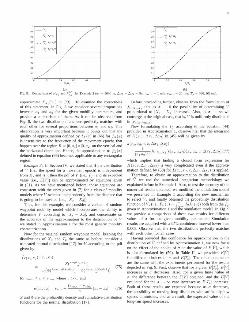
approximateFX1(x1) in (73) . To examine the correctness

of this statement, in Fig. 8 we consider several proportionsbetweena1 and a2 for the given mobility parameters, andprovide a comparison of them. As it can be observed fromFig. 8, the two distribution functions perfectly matches witheach other for several proportions betweena1 and a2. Thisobservation is very important because it points out that thequality of approximation defined byfX(x) in (66) for fX(x)is insensitive to the frequency of the movement epochs thathappen over the regionR = [0, a1]×[0, a2] on the vertical andthe horizontal directions. Hence, the approximation tofX(x)defined in equation (66) becomes applicable to any rectangularregion.

Example 3: In Section IV, we stated that if the distributionof V (i.e., the speed for a movement epoch) is independentfrom Xs andXd, then the pdf ofV (i.e., fV ) and its expectedvalue (i.e.,E[V ]) can be approximated by equations givenin (51). As we have mentioned before, those equations areconsistent with the ones given in [7] for a class of mobilitymodels whereV selected independently from the distance thatis going to be traveled (i.e.,|Xs −Xd|).

Thus, for this example, we consider a variant of randomwaypoint mobility model which incorporates the ability todetermineV according to |Xs − Xd|, and concentrate onthe accuracy of the approximation to the distribution ofVwe stated in Approximation 1 for the most generic mobilitycharacterization.

Now for the original random waypoint model, keeping thedistributions ofXd and Tp the same as before, consider atruncated normal distribution [17] forV according to the pdfgiven by

fV |Xs,Xd(v|xs, xd)

=Z(v−µ(xs,xd)

σ )

σ(

Φ(vmax−µ(xs,xd)σ ) − Φ( vmin−µ(xs,xd)

σ ))

(75)

for vmin ≤ v ≤ vmax whereσ > 0, and

µ(xs, xd) = vmin +(vmax − vmin)

a|xs − xd| (76)

Z andΦ are the probability density and cumulative distributionfunctions for the normal distribution [17].

Before proceeding further, observe from the formulation offV |Xs,Xd

that asσ → 0 the possibility of determiningVproportional to|Xs − Xd| increases. Also, asσ → ∞ weconverge to the original case, that is,V is uniformly distributedin [vmin, vmax].

Now formulating thefV according to the equation (44)provided in Approximation 1, observe first that the integrandof K(x, v,∆x1,∆x2) in (45) will be given by

k(xs, xd, x, v,∆x1,∆x2)

=1

(a1 a2)2vfV |Xs,Xd

(v|xs, xd)L(xs, xd, x,∆x1,∆x2),(77)

which implies that finding a closed form expression forK(x, v,∆x1,∆x2) is very complicated even if the approxi-mation defined by (59) forL(xs, xd, x,∆x1,∆x2) is applied.

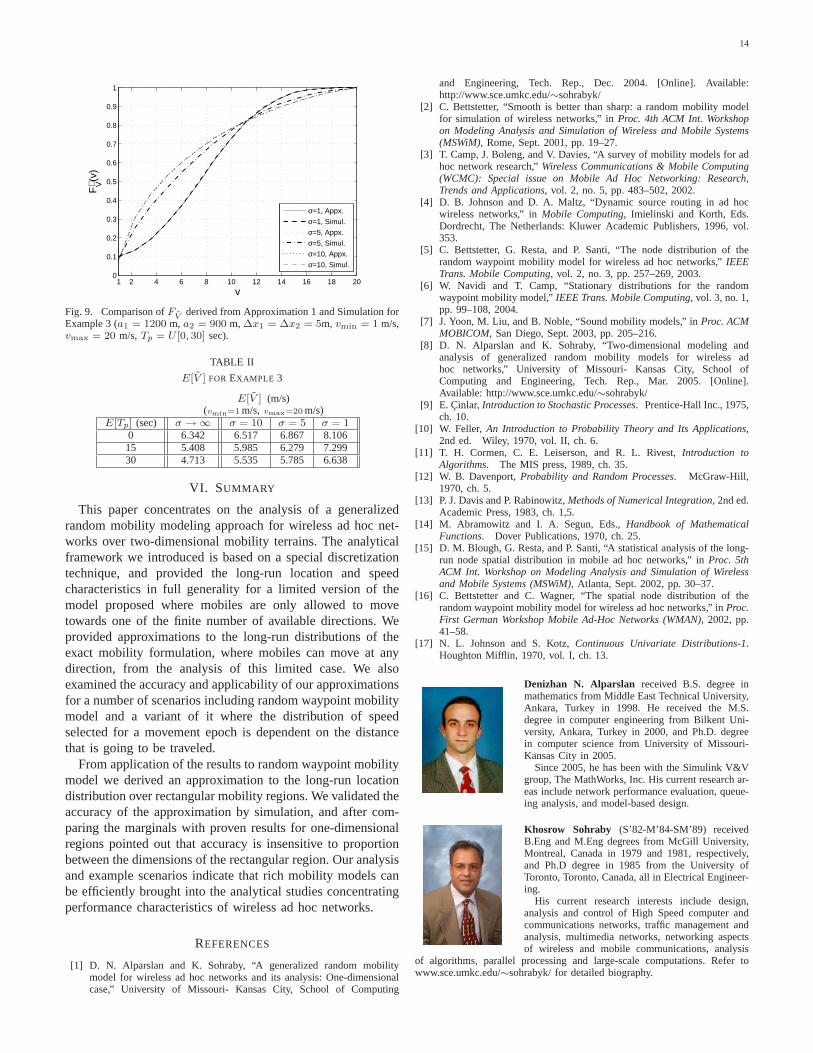
Therefore, to obtain an approximation to the distributionof V we use the numerical integration methodology weexplained before in Example 1. Also, to test the accuracy of thenumerical results obtained, we modified the simulation modelwe presented in Example 1 according the new mechanismto selectV , and finally obtained the probability distributionfunction ofV , (i.e.,FV (v) =

∫ v

vmindufV (u)) both from thefV

given in Approximation 1 and the simulation model. In Fig. 9we provide a comparison of these two results for differentvalues of σ for the given mobility parameters. Simulationresults are acquired with a95% confidence interval lower than0.003. Observe that, the two distributions perfectly matcheswith each other for all cases.

Having provided this confidence for approximation to thedistribution of V defined by Approximation 1, we now focuson the effect of the choice ofσ on the value ofE[V ], whichis also formulated by (50). In Table II, we providedE[V ]for different choices ofσ and E[Tp]. The other parametersare the same with the experiments performed for the resultsdepicted in Fig. 9. First, observe that for a givenE[Tp], E[V ]increases asσ decreases. Also, for a given finite value ofσ, the difference between theE[V ] obtained, and theE[V ]evaluated for theσ → ∞ case increases asE[Tp] increases.Both of these results are expected because asσ decreases,the possibility of moving long distances with artificially lowspeeds diminishes, and as a result, the expected value of thelong-run speed increases.

14

1 2 4 6 8 10 12 14 16 18 200

0.1

0.2

0.3

0.4

0.5

0.6

0.7

0.8

0.9

1

v

FV(v

)

∼

σ=1, Appx.

σ=1, Simul.

σ=5, Appx.

σ=5, Simul.

σ=10, Appx.

σ=10, Simul.

Fig. 9. Comparison ofFV derived from Approximation 1 and Simulation forExample 3 (a1 = 1200 m, a2 = 900 m, ∆x1 = ∆x2 = 5m, vmin = 1 m/s,vmax = 20 m/s, Tp = U [0, 30] sec).

TABLE II

E[V ] FOR EXAMPLE 3

E[V ] (m/s)(vmin=1 m/s, vmax=20 m/s)

E[Tp] (sec) σ → ∞ σ = 10 σ = 5 σ = 10 6.342 6.517 6.867 8.10615 5.408 5.985 6.279 7.29930 4.713 5.535 5.785 6.638

VI. SUMMARY

This paper concentrates on the analysis of a generalizedrandom mobility modeling approach for wireless ad hoc net-works over two-dimensional mobility terrains. The analyticalframework we introduced is based on a special discretizationtechnique, and provided the long-run location and speedcharacteristics in full generality for a limited version ofthemodel proposed where mobiles are only allowed to movetowards one of the finite number of available directions. Weprovided approximations to the long-run distributions of theexact mobility formulation, where mobiles can move at anydirection, from the analysis of this limited case. We alsoexamined the accuracy and applicability of our approximationsfor a number of scenarios including random waypoint mobilitymodel and a variant of it where the distribution of speedselected for a movement epoch is dependent on the distancethat is going to be traveled.

From application of the results to random waypoint mobilitymodel we derived an approximation to the long-run locationdistribution over rectangular mobility regions. We validated theaccuracy of the approximation by simulation, and after com-paring the marginals with proven results for one-dimensionalregions pointed out that accuracy is insensitive to proportionbetween the dimensions of the rectangular region. Our analysisand example scenarios indicate that rich mobility models canbe efficiently brought into the analytical studies concentratingperformance characteristics of wireless ad hoc networks.

REFERENCES

[1] D. N. Alparslan and K. Sohraby, “A generalized random mobilitymodel for wireless ad hoc networks and its analysis: One-dimensionalcase,” University of Missouri- Kansas City, School of Computing

and Engineering, Tech. Rep., Dec. 2004. [Online]. Available:http://www.sce.umkc.edu/∼sohrabyk/

[2] C. Bettstetter, “Smooth is better than sharp: a random mobility modelfor simulation of wireless networks,” inProc. 4th ACM Int. Workshopon Modeling Analysis and Simulation of Wireless and Mobile Systems(MSWiM), Rome, Sept. 2001, pp. 19–27.

[3] T. Camp, J. Boleng, and V. Davies, “A survey of mobility models for adhoc network research,”Wireless Communications & Mobile Computing(WCMC): Special issue on Mobile Ad Hoc Networking: Research,Trends and Applications, vol. 2, no. 5, pp. 483–502, 2002.

[4] D. B. Johnson and D. A. Maltz, “Dynamic source routing in adhocwireless networks,” inMobile Computing, Imielinski and Korth, Eds.Dordrecht, The Netherlands: Kluwer Academic Publishers, 1996, vol.353.

[5] C. Bettstetter, G. Resta, and P. Santi, “The node distribution of therandom waypoint mobility model for wireless ad hoc networks,”IEEETrans. Mobile Computing, vol. 2, no. 3, pp. 257–269, 2003.

[6] W. Navidi and T. Camp, “Stationary distributions for the randomwaypoint mobility model,”IEEE Trans. Mobile Computing, vol. 3, no. 1,pp. 99–108, 2004.

[7] J. Yoon, M. Liu, and B. Noble, “Sound mobility models,” inProc. ACMMOBICOM, San Diego, Sept. 2003, pp. 205–216.

[8] D. N. Alparslan and K. Sohraby, “Two-dimensional modelingandanalysis of generalized random mobility models for wireless adhoc networks,” University of Missouri- Kansas City, SchoolofComputing and Engineering, Tech. Rep., Mar. 2005. [Online].Available: http://www.sce.umkc.edu/∼sohrabyk/

[9] E. Cinlar,Introduction to Stochastic Processes. Prentice-Hall Inc., 1975,ch. 10.

[10] W. Feller, An Introduction to Probability Theory and Its Applications,2nd ed. Wiley, 1970, vol. II, ch. 6.

[11] T. H. Cormen, C. E. Leiserson, and R. L. Rivest,Introduction toAlgorithms. The MIS press, 1989, ch. 35.

[12] W. B. Davenport,Probability and Random Processes. McGraw-Hill,1970, ch. 5.

[13] P. J. Davis and P. Rabinowitz,Methods of Numerical Integration, 2nd ed.Academic Press, 1983, ch. 1,5.

[14] M. Abramowitz and I. A. Segun, Eds.,Handbook of MathematicalFunctions. Dover Publications, 1970, ch. 25.

[15] D. M. Blough, G. Resta, and P. Santi, “A statistical analysis of the long-run node spatial distribution in mobile ad hoc networks,” inProc. 5thACM Int. Workshop on Modeling Analysis and Simulation of Wirelessand Mobile Systems (MSWiM), Atlanta, Sept. 2002, pp. 30–37.

[16] C. Bettstetter and C. Wagner, “The spatial node distribution of therandom waypoint mobility model for wireless ad hoc networks,”in Proc.First German Workshop Mobile Ad-Hoc Networks (WMAN), 2002, pp.41–58.

[17] N. L. Johnson and S. Kotz,Continuous Univariate Distributions-1.Houghton Mifflin, 1970, vol. I, ch. 13.

Denizhan N. Alparslan received B.S. degree inmathematics from Middle East Technical University,Ankara, Turkey in 1998. He received the M.S.degree in computer engineering from Bilkent Uni-versity, Ankara, Turkey in 2000, and Ph.D. degreein computer science from University of Missouri-Kansas City in 2005.

Since 2005, he has been with the Simulink V&Vgroup, The MathWorks, Inc. His current research ar-eas include network performance evaluation, queue-ing analysis, and model-based design.

Khosrow Sohraby (S’82-M’84-SM’89) receivedB.Eng and M.Eng degrees from McGill University,Montreal, Canada in 1979 and 1981, respectively,and Ph.D degree in 1985 from the University ofToronto, Toronto, Canada, all in Electrical Engineer-ing.

His current research interests include design,analysis and control of High Speed computer andcommunications networks, traffic management andanalysis, multimedia networks, networking aspectsof wireless and mobile communications, analysis

of algorithms, parallel processing and large-scale computations. Refer towww.sce.umkc.edu/∼sohrabyk/ for detailed biography.