RaSE: Random Subspace Ensemble Classification - Yang Feng
93
Journal of Machine Learning Research 22 (2021) 1-93 Submitted 6/20; Revised 1/21; Published 1/21 RaSE: Random Subspace Ensemble Classification Ye Tian [email protected] Department of Statistics Columbia University New York, NY 10027, USA Yang Feng [email protected] Department of Biostatistics, School of Global Public Health New York University New York, NY 10003, USA Editor: Jie Peng Abstract We propose a flexible ensemble classification framework, Random Subspace Ensemble (RaSE), for sparse classification. In the RaSE algorithm, we aggregate many weak learners, where each weak learner is a base classifier trained in a subspace optimally selected from a col- lection of random subspaces. To conduct subspace selection, we propose a new criterion, ratio information criterion (RIC), based on weighted Kullback-Leibler divergence. The theoretical analysis includes the risk and Monte-Carlo variance of the RaSE classifier, es- tablishing the screening consistency and weak consistency of RIC, and providing an upper bound for the misclassification rate of the RaSE classifier. In addition, we show that in a high-dimensional framework, the number of random subspaces needs to be very large to guarantee that a subspace covering signals is selected. Therefore, we propose an iterative version of the RaSE algorithm and prove that under some specific conditions, a smaller number of generated random subspaces are needed to find a desirable subspace through iteration. An array of simulations under various models and real-data applications demon- strate the effectiveness and robustness of the RaSE classifier and its iterative version in terms of low misclassification rate and accurate feature ranking. The RaSE algorithm is implemented in the R package RaSEn on CRAN. Keywords: Random Subspace Method, Ensemble Classification, Sparsity, Information Criterion, Consistency, Feature Ranking, High Dimensional Data 1. Introduction Ensemble classification is a very popular framework for carrying out classification tasks, which typically combines the results of many weak learners to form the final classification. It aims at improving both the accuracy and stability of weak classifiers and usually leads to a better performance than the individual weak classifier (Rokach, 2010). Two prominent examples of ensemble classification are bagging (Breiman, 1996, 1999) and random forest (Breiman, 2001), which focused on decision trees and aimed to improve the performance by bootstrapping training data and/or randomly selecting the splitting dimension in different trees, respectively. Boosting is another example that converts a weak learner that performs only slightly better than random guessing into a strong learner achieving arbitrary accu- c 2021 Ye Tian and Yang Feng. License: CC-BY 4.0, see https://creativecommons.org/licenses/by/4.0/. Attribution requirements are provided at http://jmlr.org/papers/v22/20-600.html.
-
Upload
khangminh22 -
Category
Documents
-
view
6 -
download
0
Transcript of RaSE: Random Subspace Ensemble Classification - Yang Feng

Journal of Machine Learning Research 22 (2021) 1-93 Submitted 6/20; Revised 1/21; Published 1/21
RaSE: Random Subspace Ensemble Classification
Ye Tian [email protected] of StatisticsColumbia UniversityNew York, NY 10027, USA
Yang Feng [email protected]
Department of Biostatistics, School of Global Public Health
New York University
New York, NY 10003, USA
Editor: Jie Peng
Abstract
We propose a flexible ensemble classification framework, Random Subspace Ensemble (RaSE),for sparse classification. In the RaSE algorithm, we aggregate many weak learners, whereeach weak learner is a base classifier trained in a subspace optimally selected from a col-lection of random subspaces. To conduct subspace selection, we propose a new criterion,ratio information criterion (RIC), based on weighted Kullback-Leibler divergence. Thetheoretical analysis includes the risk and Monte-Carlo variance of the RaSE classifier, es-tablishing the screening consistency and weak consistency of RIC, and providing an upperbound for the misclassification rate of the RaSE classifier. In addition, we show that in ahigh-dimensional framework, the number of random subspaces needs to be very large toguarantee that a subspace covering signals is selected. Therefore, we propose an iterativeversion of the RaSE algorithm and prove that under some specific conditions, a smallernumber of generated random subspaces are needed to find a desirable subspace throughiteration. An array of simulations under various models and real-data applications demon-strate the effectiveness and robustness of the RaSE classifier and its iterative version interms of low misclassification rate and accurate feature ranking. The RaSE algorithm isimplemented in the R package RaSEn on CRAN.
Keywords: Random Subspace Method, Ensemble Classification, Sparsity, InformationCriterion, Consistency, Feature Ranking, High Dimensional Data
1. Introduction
Ensemble classification is a very popular framework for carrying out classification tasks,which typically combines the results of many weak learners to form the final classification.It aims at improving both the accuracy and stability of weak classifiers and usually leadsto a better performance than the individual weak classifier (Rokach, 2010). Two prominentexamples of ensemble classification are bagging (Breiman, 1996, 1999) and random forest(Breiman, 2001), which focused on decision trees and aimed to improve the performance bybootstrapping training data and/or randomly selecting the splitting dimension in differenttrees, respectively. Boosting is another example that converts a weak learner that performsonly slightly better than random guessing into a strong learner achieving arbitrary accu-
c©2021 Ye Tian and Yang Feng.
License: CC-BY 4.0, see https://creativecommons.org/licenses/by/4.0/. Attribution requirements are providedat http://jmlr.org/papers/v22/20-600.html.
Tian and Feng
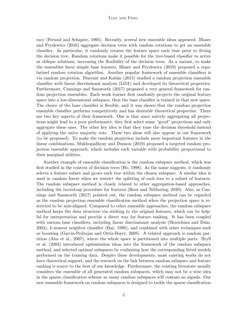
racy (Freund and Schapire, 1995). Recently, several new ensemble ideas appeared. Blaserand Fryzlewicz (2016) aggregate decision trees with random rotations to get an ensembleclassifier. In particular, it randomly rotates the feature space each time prior to fittingthe decision tree. Random rotations make it possible for the tree-based classifier to arriveat oblique solutions, increasing the flexibility of the decision trees. As a variant, to makethe ensembles favor simple base learners, Blaser and Fryzlewicz (2019) proposed a regu-larized random rotation algorithm. Another popular framework of ensemble classifiers isvia random projection. Durrant and Kaban (2015) studied a random projection ensembleclassifier with linear discriminant analysis (LDA) and developed its theoretical properties.Furthermore, Cannings and Samworth (2017) proposed a very general framework for ran-dom projection ensembles. Each weak learner first randomly projects the original featurespace into a low-dimensional subspace, then the base classifier is trained in that new space.The choice of the base classifier is flexible, and it was shown that the random projectionensemble classifier performs competitively and has desirable theoretical properties. Thereare two key aspects of their framework. One is that since naıvely aggregating all projec-tions might lead to a poor performance, they first select some “good” projections and onlyaggregate these ones. The other key idea is that they tune the decision threshold insteadof applying the naıve majority vote. These two ideas will also appear in our framework(to be proposed). To make the random projection include more important features in thelinear combinations, Mukhopadhyay and Dunson (2019) proposed a targeted random pro-jection ensemble approach, which includes each variable with probability proportional totheir marginal utilities.
Another example of ensemble classification is the random subspace method, which wasfirst studied in the context of decision trees (Ho, 1998). As the name suggests, it randomlyselects a feature subset and grows each tree within the chosen subspace. A similar idea isused in random forest when we restrict the splitting of each tree to a subset of features.The random subspace method is closely related to other aggregation-based approaches,including the bootstrap procedure for features (Boot and Nibbering, 2020). Also, as Can-nings and Samworth (2017) pointed out, the random subspace method can be regardedas the random projection ensemble classification method when the projection space is re-stricted to be axis-aligned. Compared to other ensemble approaches, the random subspacemethod keeps the data structure via sticking to the original features, which can be help-ful for interpretation and provide a direct way for feature ranking. It has been coupledwith various base classifiers, including linear discriminant analysis (Skurichina and Duin,2002), k-nearest neighbor classifier (Bay, 1998), and combined with other techniques suchas boosting (Garcıa-Pedrajas and Ortiz-Boyer, 2008). A related approach is random par-tition (Ahn et al., 2007), where the whole space is partitioned into multiple parts. Bryllet al. (2003) introduced optimization ideas into the framework of the random subspacemethod, and selected optimal subspaces by evaluating how the corresponding fitted modelsperformed on the training data. Despite these developments, most existing works do nothave theoretical support, and the research on the link between random subspace and featureranking is scarce to the best of our knowledge. Furthermore, the existing literature usuallyconsiders the ensemble of all generated random subspaces, which may not be a wise ideain the sparse classification scheme as many random subspaces will contain no signals. Ournew ensemble framework on random subspaces is designed to tackle the sparse classification
2
RaSE: Random Subspace Ensemble Classification
problems with theoretical guarantees. Instead of naively aggregating all generated randomsubspaces, we divide them into groups and only keep the “optimally” performing subspaceinside each group to construct the ensemble classifier.
Feature ranking and selection are of critical importance in many real-world applications.For example, in disease diagnosis, beyond getting an accurate prediction for patients, weare also interested in understanding how each feature contributes to our prediction, whichcan facilitate the advancement of medical science. It has been widely acknowledged that inmany high-dimensional classification problems, we only have a handful of useful features,with the rest being irrelevant ones. This is sometimes referred to as the sparse classificationproblem, which we briefly review next. Bickel et al. (2004) showed that linear discriminantanalysis (LDA) is equivalent to random guessing in the worst scenario when the sample sizeis smaller than the dimensionality. Exploiting the underlying sparsity plays a significant rolein improving the performance of the classic methods, including the LDA and the quadraticdiscriminant analysis (QDA) (Mai et al., 2012; Jiang et al., 2018; Hao et al., 2018; Fan et al.,2012; Shao et al., 2011; Fan et al., 2015; Li and Shao, 2015). While those methods workwell under their corresponding models, it is not clear how to conduct feature ranking withother types of base classifiers. In this work, we propose a flexible ensemble classificationframework, named Random Subspace Ensemble (RaSE), which can be combined with anybase classifiers and provide feature ranking as a by-product.
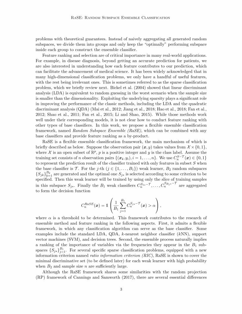
RaSE is a flexible ensemble classification framework, the main mechanism of which isbriefly described as below. Suppose the observation pair (x, y) takes values from X ×0, 1,where X is an open subset of Rp, p is a positive integer and y is the class label. Assume thetraining set consists of n observation pairs (xi, yi), i = 1, . . . , n. We use CS−Tn (x) ∈ 0, 1to represent the prediction result of the classifier trained with only features in subset S whenthe base classifier is T . For the j-th (j ∈ 1, . . . , B1) weak learner, B2 random subspacesSjkB2
k=1 are generated and the optimal one Sj∗ is selected according to some criterion to bespecified. Then this weak learner will be trained by using only the slice of training samples
in this subspace Sj∗. Finally the B1 weak classifiers CS1∗−Tn , . . . , C
SB1∗−Tn are aggregated
to form the decision function
CRaSEn (x) = 1
1
B1
B1∑j=1
CSj∗−Tn (x) > α
,
where α is a threshold to be determined. This framework contributes to the research ofensemble method and feature ranking in the following aspects. First, it admits a flexibleframework, in which any classification algorithm can serve as the base classifier. Someexamples include the standard LDA, QDA, k-nearest neighbor classifier (kNN), supportvector machines (SVM), and decision trees. Second, the ensemble process naturally impliesa ranking of the importance of variables via the frequencies they appear in the B1 sub-spaces Sj∗B1
j=1. For several specific sparse classification problems, equipped with a newinformation criterion named ratio information criterion (RIC), RaSE is shown to cover theminimal discriminative set (to be defined later) for each weak learner with high probabilitywhen B2 and sample size n are sufficiently large.
Although the RaSE framework shares some similarities with the random projection(RP) framework of Cannings and Samworth (2017), there are several essential differences
3

Tian and Feng
between them. First, the key workhorse behind RaSE is to search for a desirable subspacethat covers the signals, which makes it amenable for feature ranking and selection. TheRP framework, on the other hand, is not naturally designed for feature ranking. Second, akey condition (Assumption 2 in Cannings and Samworth (2017)) to guarantee the successof RP implies that using the criterion for choosing the optimal random projection, eachrandom projection does not deviate much from the optimal one with a non-zero probabilitythat is independent of n and p, which may not be satisfied under the high-dimensionalsetting. RaSE, however, assumes a set of conditions that explicitly take into account thehigh-dimensionality, which leads to the screening consistency and weak consistency. Third,we propose a new information criterion RIC with its theoretical properties analyzed underthe high-dimensional setting. Fourth, motivated by the stringent requirement of a large B2
for the vanilla RaSE (see Sections 3.2 and 3.5), we propose the iterative RaSE, which relaxesthe requirement on B2 by taking advantage of the feature ranking in preceding steps.
The rest of this paper is organized as follows. In Section 2, we first introduce the RaSEalgorithm, and discuss some important concepts, including minimal discriminative set andRIC. At the end of Section 2, an iterative version of the RaSE algorithm is presented. InSection 3, theoretical properties of RaSE and RIC are investigated, including the impactof B1 on the risk and Monte-Carlo variance of RaSE classifier, the screening consistencyand weak consistency of RIC, the upper bound of expected misclassification rate, and thetheoretical analysis for iterative RaSE algorithm. In Section 4, we discuss several importantcomputational issues in the RaSE algorithm, tuning parameter selection, and how to applythe RaSE framework for feature ranking. Section 5 focuses on numerical studies in terms ofextensive simulations and several real data applications, through which we compare RaSEwith various competing methods. The results frequently feature RaSE classifiers amongthe top-ranked methods and also shows its effectiveness in feature ranking. Finally, wesummarize our contributions and point out a few potential directions for future work inSection 6. We present some additional results for empirical studies in Appendix A, and allproofs are relegated to Appendix B.
2. Methodology
Recall that we have n pairs of observations (xi, yi), i = 1, . . . , n i.i.d.∼ (x, y) ∈ X × 0, 1,where X is an open subset of Rp, p is a positive integer and y ∈ 0, 1 is the class label. Weuse SFull = 1, . . . , p to represent the whole feature set. We assume the marginal densitiesof x for class 0 (y = 0) and 1 (y = 1) exist and are denoted as f (0) and f (1), respectively.The corresponding probability measures they induce are denoted as P(0) and P(1). Thus,the joint distribution of (x, y) can be described in the following mixture model
x|y = y0 ∼ (1− y0)f (0) + y0f(1), y0 = 0, 1, (1)
where y is a Bernoulli variable with success probability π1 = 1−π0 ∈ (0, 1). For any subspaceS, we use |S| to denote its cardinality. Denote Px as the probability measure induced bythe marginal distribution of x, which is in fact π0P(0) + π1P(1). When restricting to thefeature subspace S, the corresponding marginal densities of class 0 and 1 are denoted as
f(0)S and f
(1)S , respectively.
4

RaSE: Random Subspace Ensemble Classification
2.1 Random Subspace Ensemble Classification (RaSE)
Motivated by Cannings and Samworth (2017), to train each weak learner (e.g., the j-th one),B2 independent random subspaces are generated as Sj1, . . . , SjB2 . Then, according to somespecific criterion (to be introduced in Section 2.3), the optimal subspace Sj∗ is selectedand the j-th weak learner is trained only in Sj∗. Subsequently, B1 such weak classifiers
CSj∗−Tn B1j=1 are obtained. Finally, we aggregate outputs of CSj∗−Tn B1
j=1 to form the finaldecision function by taking a simple average. The whole procedure can be summarized inthe following algorithm.
Algorithm 1: Random subspace ensemble classification (RaSE)
Input: training data (xi, yi)ni=1, new data x, subspace distribution D, criterionC, integers B1 and B2, type of base classifier T
Output: predicted label CRaSEn (x), the selected proportion of each feature η1 Independently generate random subspaces Sjk ∼ D, 1 ≤ j ≤ B1, 1 ≤ k ≤ B2
2 for j ← 1 to B1 do
3 Select the optimal subspace Sj∗ from SjkB2k=1 according to C and T
4 end
5 Construct the ensemble decision function νn(x) = 1B1
∑B1j=1C
Sj∗−Tn (x)
6 Set the threshold α according to (2)7 Output the predicted label CRaSEn (x) = 1(νn(x) > α), the selected proportion of
each feature η = (η1, . . . , ηp)T where ηl = B−1
1
∑B1j=1 1(l ∈ Sj∗), l = 1, . . . , p
In Algorithm 1, the subspace distribution D is chosen as a hierarchical uniform distribu-tion over the subspaces by default. Specifically, with D as the upper bound of the subspacesize1, we first generate the subspace size d from the uniform distribution over 1, . . . , D.Then, the subspace S11 follows the uniform distribution over S ⊆ SFull : |S| = d. Inpractice, the subspace distribution can be adjusted if we have prior information about thedata structure.
In Step 6 of Algorithm 1, we set the decision threshold to minimize the empirical clas-sification error on the training set,
α = arg minα∈[0,1]
[π0(1− G(0)n (α)) + π1G
(1)n (α)], (2)
where
nr =n∑i=1
1(yi = r), r = 0, 1,
πr =nrn, r = 0, 1,
G(r)n (α) =
1
nr
n∑i=1
1(yi = r)1(νn(xi) ≤ α), r = 0, 1,
1. How to set D in practice will be discussed in Section 4.1.
5

Tian and Feng
νn(xi) =1
B1
B1∑j=1
1(CSj∗n (xi) = 1).
2.2 Minimal Discriminative Set
For sparse classification problems, it is of significance to accurately separate signals fromnoises. Motivated by Kohavi et al. (1997) and Zhang and Wang (2011), we define thediscriminative set and study some of its properties as follows.
Definition 1 A feature subset S is called a discriminative set if y is conditionally inde-pendent with xSc given xS, where Sc = SFull \ S. We call S a minimal discriminativeset if it has minimal cardinality among all discriminative sets.
Assumption 1 The densities f (0) and f (1) have the same support a.s. with respect to Px.
Remark 2 Note that the existence of densities and the common support requirement arenot necessary for the definition of the minimal discriminative set and the RaSE framework.We focus on the continuous distribution purely for notation convenience. We will discussthis assumption again after introducing our information criterion in Definition 6.
Proposition 3 Under Assumption 1, we can characterize the discriminative set using themarginal density ratio due to the following two facts.
(i) If S is a discriminative set, then
f (1)(x)
f (0)(x)=f
(1)S (xS)
f(0)S (xS)
almost surely with respect to Px.
(ii) If for a feature subset S, there exists a function h : R|S| → [0,+∞] such that
f (1)(x)
f (0)(x)= h(xS)
almost surely with respect to Px, then S is a discriminative set and
h(xS) =f
(1)S (xS)
f(0)S (xS)
almost surely with respect to Px.
In general, there may exist more than one minimal discriminative sets. For instance, iftwo features are exactly the same, then more than one minimal discriminative sets may existsince we cannot distinguish between them. To rule out this type of degenerate scenario, weimpose the uniqueness assumption for the minimum discriminative set.
Assumption 2 There is only one minimal discriminative set, which is denoted as S∗. Inaddition, all discriminative sets cover S∗.
6

RaSE: Random Subspace Ensemble Classification
In the classification problem, we are often interested in the risk of a classifier C. Withthe 0-1 loss, the risk or the misclassification rate is defined as
R(C) = E[1(C(x) 6= y)] = P(C(x) 6= y).
The Bayes classifier
CBayes(x) =
1, P(y = 1|x) > 1
2 ,
0, otherwise.(3)
is known to achieve the minimal risk among all classifiers (Devroye et al., 2013). If only fea-tures in S are used, it will provide us a “local” Bayes classifier CSBayes(xS) which achieves theminimal risk among all classifiers using only features in S. In general, there is no guaranteethat R(CSBayes) = R(CBayes). Fortunately, the equation holds when S is a discriminativeset.
Proposition 4 For any discriminative set S, it holds that
R(CSBayes) = R(CS∗
Bayes) = R(CBayes).
This direct result illustrates that covering S∗ is sufficient to obtain performance as good asthe Bayes classifier.
To clarify the notions above, we next take the two-class Gaussian settings as examplesand investigate what S∗ is in each case.
Example 1 (LDA) Suppose f (0) ∼ N(µ(0),Σ), f (1) ∼ N(µ(1),Σ), where Σ is positivedefinite. The log-density ratio is
log
(f (0)(x)
f (1)(x)
)= C − (µ(1) − µ(0))TΣ−1x,
where C is a constant independent of x. By Proposition 3, the minimal discriminative setS∗ = j : [Σ−1(µ(1) − µ(0))]j 6= 0.
This definition is equivalent to that in Mai et al. (2012) for the LDA case.
Example 2 (QDA) Suppose f (0) ∼ N(µ(0),Σ(0)), f (1) ∼ N(µ(1),Σ(1)), where Σ(0) andΣ(1) are positive definite matrices with Σ(0) 6= Σ(1), then the log-density ratio is
log
(f (0)(x)
f (1)(x)
)= C+
1
2xT[(Σ(1))−1 − (Σ(0))−1
]x+
[(Σ(0))−1µ(0) − (Σ(1))−1µ(1)
]Tx, (4)
where C is a constant independent of x. Let S∗l = j : [(Σ(0))−1µ(0) − (Σ(1))−1µ(1)]j 6= 0,S∗q = j : [(Σ(1))−1 − (Σ(0))−1]ij 6= 0, ∃i. The elements in S∗l are often called variableswith main effects while elements in S∗q are called variables with quadratic effects (Hao et al.,2018; Fan et al., 2015; Jiang et al., 2018). By Proposition 3, the minimal discriminativeset S∗ = S∗l ∪ S∗q .
Proposition 5 If f (0) ∼ N(µ(0),Σ(0)), f (1) ∼ N(µ(1),Σ(1)), where Σ(0) and Σ(1) are posi-tive definite matrices, then the following conclusions hold:
7

Tian and Feng
(i) The minimal discriminative set S∗ is unique;
(ii) For any discriminative set S, we have S ⊇ S∗;
(iii) Any set S ⊇ S∗ is a discriminative set. This conclusion also holds without the Gaus-sian assumption.
2.3 Ratio Information Criterion (RIC)
As discussed in Section 2.2, it is desirable to identify the minimal discriminative set S∗ forthe classifier to achieve a low misclassification rate. Hence in Algorithm 1, it is important toapply a proper criterion to select the “optimal” subspace. In the variable selection literature,a criterion enjoying the property of correctly selecting the minimal discriminative set withhigh probability is often referred to as a “consistent” one. For model (1), Zhang and Wang(2011) proved that BIC, in conjunction with a backward elimination procedure, is selec-tion consistent in the Gaussian mixture case. However, the BIC they investigated involvedthe joint log-likelihood function for (x, y), which involves estimating high-dimensional co-variance matrices that could be problematic when p is close to or larger than n withoutadditional structural assumptions.
Here we propose a new criterion, which enjoys the weak consistency under the generalsetting of (1), based on Kullback-Leibler divergence (Kullback and Leibler, 1951). Twoasymmetric Kullback-Leibler divergences for densities f and g are defined as
KL(f ||g) = Ex∼f
[log
(f(x)
g(x)
)],KL(g||f) = Ex∼g
[log
(g(x)
f(x)
)],
where Ex∼f represents taking expectation with respect to x ∼ f . In binary classificationmodel (1), marginal probabilities can be crucial because imbalanced marginal distributionscan significantly compromise the performance of most standard learning algorithms (Heand Garcia, 2009). Therefore, we consider a weighted version of two KL divergences for the
marginal distributions f(0)S and f
(1)S with subspace S, i.e. π0KL(f
(0)S ||f
(1)S )+π1KL(f
(1)S ||f
(0)S ).
Denote by f(0)S , f
(1)S , π0, π1 the estimated version via MLEs of parameters, then it holds that
π0KL(f(0)S ||f
(1)S ) = n−1
n∑i=1
1(yi = 0) · log
[f
(0)S (xi,S)
f(1)S (xi,S)
],
π1KL(f(1)S ||f
(0)S ) = n−1
n∑i=1
1(yi = 1) · log
[f
(1)S (xi,S)
f(0)S (xi,S)
].
Now, we are ready to introduce the following new criterion named ratio information crite-rion (RIC), with a proper penalty term.
Definition 6 For model (1), the ratio information criterion (RIC) for feature subspace Sis defined as
RICn(S) = −2[π0KL(f(0)S ||f
(1)S ) + π1KL(f
(1)S ||f
(0)S )] + cn · deg(S), (5)
where cn is a function of sample size n and deg(S) is the degree of freedom correspondingto the model with subspace S.
8

RaSE: Random Subspace Ensemble Classification
Remark 7 Assumption 1 is necessary to make sure RIC is well-defined. To see this, notethat the existence of both Kullback-Leibler divergences requires (1) f (0)(x) = 0⇒ f (1)(x) =0 a.s. with respect to P(1); (2) f (1)(x) = 0⇒ f (0)(x) = 0 a.s. with respect to P(0). This isequivalent to Assumption 1 when π0, π1 > 0.
Note that although AIC is also motivated by the Kullback-Leibler divergence, it aims tominimize the KL divergence between the estimated density and the true density (Burnhamand Anderson, 1998). In our case, however, the goal is to maximize the KL divergencebetween the conditional densities under two classes to achieve a greater separation.
Next, let’s work out a few familiar examples where explicit expressions exist for RIC.
Proposition 8 (RIC for the LDA model) Suppose f (0) ∼ N(µ(0),Σ), f (1) ∼ N(µ(1),Σ),where Σ is positive definite. The MLEs of the parameters are
µ(r)S =
1
nr
n∑i=1
1(yi = r)xi,S , r = 0, 1,
ΣS,S =1
n
n∑i=1
1∑r=0
1(yi = r) · (xi,S − µ(r)S )(xi,S − µ(r)
S )T ,
Then we have
RICn(S) = −(µ(1)S − µ
(0)S )T Σ−1
S,S(µ(1)S − µ
(0)S ) + cn(|S|+ 1).
Proposition 9 (RIC for the QDA model) Suppose f (0) ∼ N(µ(0),Σ(0)), f (1) ∼ N(µ(1),Σ(1)),where Σ(0), Σ(1) are positive definite but not necessarily equal. The MLEs of the estimators
are as follows. µ(r)S , r = 0, 1 are the same as in Proposition 8, and
Σ(r)S,S =
1
nr
n∑i=1
1(yi = r) · (xi,S − µ(r)S )(xi,S − µ(r)
S )T , r = 0, 1.
Then we have
RICn(S) = −(µ(1)S − µ
(0)S )T [π1(Σ
(0)S,S)−1 + π0(Σ
(1)S,S)−1](µ
(1)S − µ
(0)S )
+ Tr[((Σ(1)S,S)−1 − (Σ
(0)S,S)−1)(π1Σ
(1)S,S − π0Σ
(0)S,S)] + (π1 − π0)(log |Σ(1)
S,S | − log |Σ(0)S,S |)
+ cn ·[|S|(|S|+ 3)
2+ 1
].
Note that the primary term of RIC for the LDA case, is the Mahalanobis distance(McLachlan, 1999), which is closely related to the Bayes error of LDA classifier (Efron,1975). And for the QDA case, the KL divergence components contain three terms. The firstterm is similar to the Mahalanobis distance, representing the contributions of linear signalsto the classification model. And the second and third terms represent the contributions ofquadratic signals.
Note that the KL divergence can also be estimated by non-parametric methods includ-ing the k-nearest neighbor distance (Wang et al., 2009; Ganguly et al., 2018), which may
9

Tian and Feng
sometimes lead to more robust estimates than the parametric ones in our numerical exper-
iments. Specifically, consider two samples x(0)i,S
n0i=1
i.i.d.∼ f(0)S and x(1)
i,Sn1i=1
i.i.d.∼ f(1)S , and
write ρk0,0(x(0)j,S) for the Euclidean distance between x
(0)j,S and its k0-th nearest neighbor in
the sample x(0)i,S
n0i=1\x
(0)j,S, and write ρk1,1(x
(0)j,S) for the Euclidean distance between x
(0)j,S
and its k1-th nearest neighbor in the sample x(1)i,S
n1i=1. Wang et al. (2009) and Ganguly
et al. (2018) defined the following asymptotic unbiased estimator given k0 and k1:
KL(f(0)S ||f
(1)S ) =
|S|n0
n0∑i=1
log
ρk0,0(x(0)i,S)
ρk1,1(x(0)i,S)
+ log
(n1
n0 − 1
)+ Ψ(k0)−Ψ(k1), (6)
where Ψ denotes the diGamma function (Abramowitz and Stegun, 1948). Similarly we can
obtain estimate KL(f(1)S ||f
(0)S ). Besides, Berrett and Samworth (2019) proposed a weighted
estimator based on (6) and investigated its efficiency. We will compare the performance ofRaSE when using the estimate in (6) to that using parametric methods in simulation.
Another line of research for classification is to study the conditional distribution ofy|x. For this setup, there has been a rich literature on various information type criteriathat involves the conditional log-likelihood function. Akaike information criterion (AIC)(Akaike, 1973) was shown to be inconsistent. It was demonstrated that Bayesian informationcriterion (BIC) is consistent under certain regularity conditions (Rao and Wu, 1989). Chenand Chen (2008, 2012) modified the definition of conventional BIC to form the extendedBIC (eBIC) for the high-dimensional setting where p grows at a polynomial rate of n. Fanand Tang (2013) proved the consistency of a generalized information criterion (GIC) forgeneralized linear models in ultra-high dimensional space.
2.4 Iterative RaSE
The success of the RIC proposed in Section 2.3 relies on the assumption that the minimaldiscriminative set S∗ appears in some of the B2 subspaces for each weak learner. Forsparse classification problems, the size of S∗ can be very small compared to p. Whenp is large, the probability of generating a subset that covers S∗ is quite low accordingto the hierarchical uniform distribution for subspaces. It turns out by using the selectedfrequency of each feature in B1 subspaces Sj∗B1
j=1 from Algorithm 1, we can improve theRaSE algorithm by running the RaSE algorithm again with a new hierarchical distributionfor subspaces. In particular, we first calculate the percentage vector η = (η1, . . . , ηp)
T
representing the proportion of each feature appearing among B1 subspaces Sj∗B1j=1, where
ηl = B−11
∑B1j=1 1(l ∈ Sj∗), l = 1, . . . , p. The new hierarchical distribution is specified as
follows. In the first step, we generate the subspace size d from the uniform distribution over1, . . . , D as before. Before moving on to the second step, note that each subspace S canbe equivalently represented as J = (J1, . . . , Jp)
T , where Jl = 1(l ∈ S), l = 1, . . . , p. Then,we generate J from a restrictive multinomial distribution with parameter (p, d, η), whereη = (η1, . . . , ηp)
T , ηl = ηl1(ηl > C0/ log p) + C0p 1(ηl ≤ C0/ log p), and the restriction is that
Jl ∈ 0, 1, l = 1, . . . , p. Here C0 is a constant.Intuitively, this strategy can be repeated to increase the probability that signals in
S∗ are covered in the subspaces we generate. It could also lead to an improved feature
10

RaSE: Random Subspace Ensemble Classification
ranking according to the updated proportion of each feature η. This will be verified viamultiple simulation experiments in Section 5. This iterative RaSE algorithm is summarizedin Algorithm 2.
A related idea was introduced by Mukhopadhyay and Dunson (2019) to generate randomprojections with probabilities proportional to the marginal utilities. One major differencein RaSE is that the feature importance is determined via their joint contributions in theselected subspaces.
Algorithm 2: Iterative RaSE (RaSET )
Input: training data (xi, yi)ni=1, new data x, initial subspace distribution D(0),criterion C, integers B1 and B2, the type of base classifier T , the number ofiterations T
Output: predicted label CRaSEn (x), the proportion of each feature η(T )
1 for t← 0 to T do
2 Independently generate random subspaces S(t)jk ∼ D
(t), 1 ≤ j ≤ B1, 1 ≤ k ≤ B2
3 for j ← 1 to B1 do
4 Select the optimal subspace S(t)j∗ from S(t)
jk B2k=1 according to C and T
5 end
6 Update η(t) where η(t)l = B−1
1
∑B1j=1 1(l ∈ S(t)
j∗ ), l = 1, . . . , p
7 Update D(t) ← restrictive multinomial distribution with parameter (p, d, η(t)),
where η(t)l = η
(t)l 1(η
(t)l > C0/ log p) + C0
p 1(η(t)l ≤ C0/ log p) and d is sampled
from the uniform distribution over 1, . . . , D8 end9 Set the threshold α according to (2)
10 Construct the ensemble decision function νn(x) = 1B1
∑B1j=1C
S(T )j∗ −T
n (x)
11 Output the predicted label CRaSEn (x) = 1(νn(x) > α) and η(T )
3. Theoretical Studies
In this section, we investigate various theoretical properties of RaSE, including the impactof B1 on the risk of RaSE classifier and expectation of misclassification rate. Furthermore,we will demonstrate that RIC achieves weak consistency. Throughout this section, we allowthe dimension p grows with sample size n.
To streamline the presentation, we first introduce some additional notations. In thispaper, we have three different sources of randomness: (1) the randomness of the trainingdata, (2) the randomness of the subspaces, and (3) the randomness of the test data. Wewill use the following notations to differentiate them.
• Analogous to Cannings and Samworth (2017), we write P and E to represent theprobability and expectation with respect to the collection of B1B2 random subspacesSjk : 1 ≤ j ≤ B1, 1 ≤ k ≤ B2;
• P and E are used when the randomness comes from the training data (xi, yi)ni=1;
11

Tian and Feng
• We use P and E when considering all three sources of randomness.
Recall that in Algorithm 1, the decision function is
νn(x) =1
B1
B1∑j=1
CSj∗n (x).
For a given threshold α ∈ (0, 1), the RaSE classifier is
CRaSEn (x) =
1, νn(x) > α,
0, νn(x) ≤ α.
By the weak law of large numbers, as B1 → ∞, νn will converge in probability to itsexpectation
µn(x) = P(CS1∗n (x) = 1
).
It should be noted that here as both the training data and the criterion C in Algorithm 1are fixed, S1∗ is a deterministic function of S1kB2
k=1. Nevertheless, µn(x) is still randomdue to randomness of the new x. Then, it is helpful to define the conditional cumulative
distribution function of µn for class 0, 1 respectively as G(0)n (α′) = P(µn(x) ≤ α′|y =
0) = P(0)(µn(x) ≤ α′) and G(1)n (α′) = P(µn(x) ≤ α′|y = 1) = P(1)(µn(x) ≤ α′). Since
the distribution D of subspaces is discrete, µn(x) takes finite unique values almost surely,
implying G(0)n , G
(1)n to be step functions. We denote the corresponding probability mass
functions of G(0)n and G
(1)n as g
(0)n and g
(1)n , respectively. Since for any x, νn(x)→ µn(x) as
B1 →∞, we consider the following randomized RaSE classifier in population
CRaSE∗n (x) =
1, µn(x) > α,
0, µn(x) < α,
Bernoulli(
12
), µn(x) = α.
as the infinite simulation RaSE classifier with B1 →∞.In the following sections, we would like to study different properties of CRaSEn . In
Section 3.1, we condition on the training data and study the impact ofB1 via the relationshipbetween test error of CRaSEn and CRaSE∗n and Monte-Carlo variance Var(R(CRaSEn )), whichcan reflect the stability of RaSE classifier as B1 increases. It will be demonstrated thatconditioned on training data, both the difference between the test errors of CRaSEn andCRaSE∗n , and the Monte-Carlo variance of CRaSEn , converge to zero as B1 → ∞ for almostevery threshold α ∈ (0, 1) at an exponential rate. In Section 3.3, we will prove an upperbound for the expected misclassification rate R(CRaSEn ) with respect to all the randomnessfor fixed threshold α. Next, we introduce several scaling notations. For two sequences anand bn, we use an = o(bn) or an bn to denote |an/bn| → 0; an = O(bn) or an . bnto denote |an/bn| < ∞. The corresponding stochastic scaling notations are op and Op,
where an = op(bn), an = Op(bn) imply that |an/bn|p−→ 0 and for any ε > 0, there exists
M > 0 such that P(|an/bn| > M) ≤ ε, ∀n. Also, we use λmin(A) and λmax(A) to denote thesmallest and largest eigenvalues of a square matrix A. For any vector x = (x1, . . . , xp)
T , the
Euclidean norm ‖x‖ =√∑
i x2i . And for any matrix A = (aij)p×p, we define the operator
12

RaSE: Random Subspace Ensemble Classification
norm ‖A‖2 = sup‖x‖2=1
‖Ax‖2, the infinity norm ‖A‖∞ = supi
∑pj=1 |aij |, the maximum norm
‖A‖max = maxi,j|aij |, and the Frobenius norm ‖A‖F =
√∑i,j a
2ij .
3.1 Impact of B1
In this section, we study the impact of B1 by presenting upper bounds of the absolutedifference between the test error of CRaSEn and CRaSE∗n , and Monte-Carlo variance for RaSEwhen conditioned on the training data as B1 grows. Note that the discrete distribution ofrandom subspaces leads to both bounds vanishing at exponential rates, except for a finiteset of thresholds α, which is very appealing.
Theorem 10 (Risk for the RaSE classifier conditioned on training data) Denote
Gn(α′) = π1G(1)n (α′) − π0G
(0)n (α′) and αiNi=1 represents the discontinuity points of Gn.
Given training samples with size n, we have the following bound for expected misclassifica-tion rate of RaSE classifier with threshold α when B1 →∞ as
|E[R(CRaSEn )]−R(CRaSE∗n )| ≤
O(
1√B1
), α ∈ αiNi=1,
exp −CαB1 , otherwise,
where Cα = 2 min1≤i≤N
(|α− αi|2).
It shows that as B1 →∞, the RaSE classifier CRaSEn and its infinite simulation versionCRaSE∗n achieve the same expected misclassification rate conditioned on the training data.Many similar results about the excess risk of randomized ensembles have been studied inliterature (Cannings and Samworth, 2017; Lopes et al., 2019; Lopes, 2020). Next, we providea similar upper bound for the MC variance of the RaSE classifier. Suppose the discontinuity
points of G(0)n and G
(1)n are α0
i N0i=1 and α1
jN1j=1, respectively.
Theorem 11 (MC variance for the RaSE classifier) It holds that
Var[R(CRaSEn )] ≤
12
[π0(g
(0)n (α))2 + π1(g
(1)n (α))2
]+O
(1√B1
), α ∈ α(0)
i N0i=1 ∪ α
(1)j
N1j=1
exp −CαB1 , otherwise,
where Cα = 2 min1≤i≤N01≤j≤N1
(|α− α(0)i |2, |α− α
(1)j |2).
This theorem asserts that except for a finite set of threshold α, the MC variance of RaSEclassifier shrinks to zero at an exponential rate.
3.2 Theoretical Properties of RIC
An important step of the RaSE classifier is the choice of an “optimal” subspace among B2
subspaces for each of the B1 weak classifiers. Before showing the screening consistency andweak consistency of RIC, we first present a proposition that explains the intuition of whyRIC can succeed.
13

Tian and Feng
Proposition 12 When Assumptions 1 and 2 hold, we have the following conclusions:
(i) KL(f(0)S ||f
(1)S ) = KL(f
(0)S∗ ||f
(1)S∗ ),KL(f
(1)S ||f
(0)S ) = KL(f
(1)S∗ ||f
(0)S∗ ) hold for any S ⊇ S∗;
(ii) π0KL(f(0)S ||f
(1)S ) + π1KL(f
(1)S ||f
(0)S ) < π0KL(f
(0)S∗ ||f
(1)S∗ ) + π1KL(f
(1)S∗ ||f
(0)S∗ ) if S 6⊇ S∗;
(iii) KL(f(0)S∗ ||f
(1)S∗ ) = sup
SKL(f
(0)S ||f
(1)S ),KL(f
(1)S∗ ||f
(0)S∗ ) = sup
SKL(f
(1)S ||f
(0)S ).
From Proposition 12, if we define the population RIC without penalty as
RIC(S) = −2[π0KL(f
(0)S ||f
(1)S ) + π1KL(f
(1)S ||f
(0)S )],
it can be easily seen that supS:S⊇S∗
RIC(S) = RIC(S∗) < infS:S 6⊇S∗
RIC(S). To successfully
differentiate S∗ from S : S 6⊇ S∗ using RICn, we need to impose a condition on theminimum gap of RIC on S∗ and that on S where S 6⊇ S∗. Similar assumptions suchas the “beta-min” condition appears in the high-dimensional variable selection literature(Buhlmann and Van De Geer, 2011). Denote
ψ(n, p,D) =
√D log p+ κ1 logD
nmax
Dκ1(Dκ3 +Dκ4), Dκ5 , D2κ1+κ2
√D log p+ κ1 logD
n
.
The complete set of conditions is presented as follows.
Assumption 3 Suppose densities f (0) and f (1) are in parametric forms with f (0)(x) =f (0)(x;θ), f (1)(x) = f (1)(x;θ), where θ contains all parameters for both f (0) and f (1).Note that not all elements of θ appear in f (0) or f (1). Denote the dimension of θ as p′.As in Section 2.1, D represents the upper bound of the subspace size. Define LS(x,θ) =
log
(f
(0)S (xS ;θS)
f(1)S (xS ;θS)
). Assume the following conditions hold, where κ1, κ2, κ3, κ4, κ5 ≥ 0 and
C1, C2, C3, C4, C5 > 0 are some universal constants which does not depend on n, p or D:
(i) p′ is a function of p and p′(p) . pκ1;
(ii) max[KL(f (0)||f (1)),KL(f (1)||f (0))
]. (p∗)κ1 . Dκ1;
(iii) There exists a family of functions VS(xi,Sni=1)S where VS(xi,Sni=1) ∈ R, suchthat for ∀xi,Sni=1 ∈ X and subset S with |S| ≤ D, there exists a constant ζ such thatif ‖θ′S − θS‖2 ≤ ζ, then∥∥∥∥∥ 1
n
n∑i=1
∇2θSLS(xi,θ
′)
∥∥∥∥∥max
≤ VS(xi,Sni=1),
and the following tail probability bound holds for VS:
P (VS(xi,Sni=1) > C1Dκ2) . exp−C2n,
where xi,S ∼ f (0)S or f
(1)S ;
14

RaSE: Random Subspace Ensemble Classification
(iv) Each component of ∇θSLS(x,θ) is√
2C3Dκ3-subGaussian for any subset S with |S| ≤
D where xS ∼ f (0)S or xS ∼ f (1)
S , respectively;
(v) supS:|S|≤D
∥∥∥ExS∼f
(0)S
∇θSLS(x,θ)∥∥∥∞, supS:|S|≤D
∥∥∥ExS∼f
(1)S
∇θSLS(x,θ)∥∥∥∞
. Dκ4;
(vi) LS(x,θ) is a√
2C4Dκ5-subGaussian variable, where xS ∼ f (0)
S or xS ∼ f (1)S ;
(vii) Denoting the MLE of θ based on subset S with |S| ≤ D as
θS = arg maxθS
n∑i=1
1∑r=0
1(yi = r) log f(r)S (xi,S ;θS),
then when ε is smaller than a positive constant, it holds that
P(‖θS − θS‖∞ > ε) . |S|κ1 exp−C5nε2 ⇒ ‖θS − θS‖∞ = Op
(√κ1 log |S|
n
).
(viii) The signal strength satisfies
∆ := infS:S 6⊇S∗|S|≤D
RIC(S)− RIC(S∗) ψ(n, p,D),
where ψ(n, p,D) = o(1).
Here condition (i) assumes the number of parameters in the model grows slower than apolynomial rate of the dimension. Condition (ii) assumes an upper bound for the two KLdivergences. Conditions (iii)-(vi) are imposed to guarantee the accuracy of the second-orderapproximation for RIC. And condition (vii) is usually satisfied for common distributionfamilies (Van der Vaart, 2000). The last condition is a requirement for the signal strength.A condition of this type is necessary to prove the consistency result for any informationcriterion.
For condition (viii), it imposes a constraint among n, p, and D. When D p, it canbe simplified as
Dκ · log p
n= o(1),
where κ is some positive constant. To cover all the signals in S∗, we require D ≥ p∗.Therefore, an implied requirement for n, p, and p∗ is
(p∗)κ · log p
n= o(1),
which is similar to the conditions in the literature of variable selection. Here, we allow p togrow at an exponential rate of n.
To help readers understand these conditions better, we show that some commonly usedconditions (presented in Assumption 4) for high-dimensional LDA model are sufficient forAssumption 3.(i)-(vii) to hold with the results presented in Proposition 14. Assumption3.(viii) can be relaxed under the LDA model.
15

Tian and Feng
Assumption 4 (LDA model) Suppose the following conditions are satisfied, where m,M , M ′ are constants:
(i) λmin(Σ) ≥ m > 0, ‖Σ‖max ≤M <∞;
(ii) ‖µ(1) − µ(0)‖∞ ≤M ′ <∞;
(iii) Denote δS = Σ−1S,S(µ
(1)S − µ
(0)S ), γ = inf
j|(δS∗)j | > 0, then
γ2 D2
√log p
n= o(1).
Remark 13 Here, condition (i) constrains the eigenvalues of the common covariance ma-trix, which is similar to condition (C2) in Hao et al. (2018) and Wang (2009), condition(2) in Shao et al. (2011), condition (C4) in Li and Liu (2019). Condition (ii) imposes anupper bound for the maximal componentwise mean difference of the two classes, which issimilar to condition (3) in Shao et al. (2011). Condition (iii) assumes a lower bound on theminimum signal strength γ, which is in a similar spirit to condition 2 in Mai et al. (2012).
Proposition 14 Suppose f (0) ∼ N(µ(0),Σ), f (1) ∼ N(µ(1),Σ), where Σ is positive definite.
If Assumption 4 holds, then Assumption 3.(i)-(vii) hold with θS = ((µ(0)S )T , (µ
(1)S )T , vec(ΣS,S)T )T
and κ1 = 2, κ2 = κ4 = 1, κ3 = κ5 = 12 .
The detailed proof for this proposition can be found in Appendix B. We are now ready topresent the consistency result for RIC as defined in (5).
Theorem 15 (Consistency of RIC) Under Assumptions 1-3, we have
(i) If supS:|S|≤D
deg(S) · cn/∆ = o(1), then the following screening consistency holds for
RIC:2
P
supS:S⊇S∗|S|≤D
RICn(S) < infS:S 6⊇S∗|S|≤D
RICn(S)
≥ 1−O(pDDκ1 exp
−Cn
(∆
D2κ1+κ2
))
−O
(pDDκ1 exp
−Cn
(∆
Dκ1(Dκ3 +Dκ4)
)2)−O
(pD exp
−Cn
(∆
Dκ5
)2)
→ 1.
(ii) If in addition cn ψ(n, p,D), then the weak consistency in the following sense holdsfor RIC:
P(
RICn(S∗) = infS:|S|≤D
RICn(S)
)≥ 1−O
(pDDκ1 exp
−Cn
( cnD2κ1+κ2
))2. Note that here we assume that MLE of θ is well-defined for all models under consideration.
16

RaSE: Random Subspace Ensemble Classification
−O
(pDDκ1 exp
−Cn
(cn
Dκ1(Dκ3 +Dκ4)
)2)−O
(pD exp
−Cn
( cnDκ5
)2)
→ 1.
Corollary 16 Denote pS∗ = P(S11 ⊇ S∗) = 1D
∑p∗≤d≤D
(p−p∗
d−p∗)(pd)
, where the subspaces are
generated from the hierarchical uniform distribution. Assume the conditions stated in As-sumption 1-2 hold, and in addition there holds
B2pS∗ 1.
If we select the optimal subspace by minimizing RIC as the criterion in RaSE where D ≥ p∗,then we have
P(S1∗ ⊇ S∗) ≥ P
supS:S⊇S∗|S|≤D
RICn(S) < infS:S 6⊇S∗|S|≤D
RICn(S)
·P B2⋃j=1
S1j ⊇ S∗
, (7)
where
P
B2⋃j=1
S1j ⊇ S∗
= 1− (1− pS∗)B2 ≥ 1−O (exp −B2pS∗) .
Remark 17 Note that this corollary actually holds when we replace RICn with a generalcriterion Crn (smaller value leads to better subspace) with more discussions in Section 3.5.And for RIC, the bounds for the first probability on the right-hand side of (7) in Theorems15, 18 and 20 can be plugged in to get the explicit bounds.
Also, we want to point out that direct analyses of RIC for discriminant analysis modelsare also insightful and interesting. We can show similar consistency results as those inTheorem 15 from properties of discriminant analysis approach itself based on some commonconditions used in literature about sparse discriminant analysis, instead of applying thegeneral analysis of KL divergence.
Theorem 18 (LDA consistency) For the LDA model, under Assumption 4, we have
(i) If Dcn/γ2 = o(1), then the following screening consistency holds for RIC:
P
supS:S⊇S∗|S|≤D
RICn(S) < infS:S 6⊇S∗|S|≤D
RICn(S)
≥ 1−O
(p2 exp
−Cn
(γ2
D2
)2)→ 1.
(ii) If in addition cn D2√
log pn , then RIC is weakly consistent:
P(
RICn(S∗) = infS:|S|≤D
RICn(S)
)≥ 1−O
(p2 exp
−Cn
( cnD2
)2)→ 1.
17

Tian and Feng
Assumption 5 (QDA model) Denote Ω(r)S,S = (Σ
(r)S,S)−1, r = 0, 1. Suppose the following
conditions are satisfied, where m,M,M ′ are constants:
(i) λmin(Σ(r)) ≥ m > 0, λmax(Σ(r)) ≤M <∞, r = 0, 1;
(ii) ‖µ(1) − µ(0)‖∞ ≤M ′ <∞;
(iii) Denote γl = infj
∣∣∣(Ω(1)S,Sµ
(1)S − Ω
(0)S,Sµ
(0)S )j
∣∣∣ > 0, γq = infi
supj
∣∣∣(Ω(1)S∗q ,S
∗q− Ω
(0)S∗q ,S
∗q)ij
∣∣∣ > 0,
then
minγ2l , γ
2q , γq D2
√log p
n= o(1).
Remark 19 The conditions here are similar to Assumption 4 for the LDA model. A setof analogous conditions were used in Jiang et al. (2018).
Theorem 20 (QDA consistency) For the QDA model, under Assumption 5,
(i) If D2cn/minγ2l , γ
2q , γq = o(1), then RIC is screening consistent:
P
supS:S⊇S∗|S|≤D
RICn(S) < infS:S 6⊇S∗|S|≤D
RICn(S)
≥ 1−O
p2 exp
−Cn(
minγ2l , γ
2q , γq
D2
)2
→ 1.
(ii) Further, if cn D2√
log pn , then RIC is weakly consistent:
P(
RICn(S∗) = infS:|S|≤D
RICn(S)
)≥ 1−O
(p2 exp
−Cn
( cnD2
)2)→ 1.
The proof is available in Appendix B. Note that the bound here is tighter than the resultsfrom Proposition 14 and Theorem 15.
Based on the consistency of RIC, in the next section, we will construct an upper boundfor the expectation of the misclassification rate R(CRaSEn ).
3.3 Misclassification Rate of the RaSE Classifier
In the following theorem, we present an upper bound on the misclassification rate for theRaSE classifier, which holds for any criterion to choose optimal subspaces.
Theorem 21 (General misclassification rate) For the RaSE classifier with thresholdα and any criterion to choose optimal subspaces, it holds that
EE[R(CRaSEn )−R(CBayes)] ≤
E supS:S⊇S∗|S|≤D
[R(CSn )−R(CBayes)] + P(S1∗ 6⊇ S∗)
min(α, 1− α). (8)
18

RaSE: Random Subspace Ensemble Classification
Here, the upper bound consists of two terms. The first term involving E supS:S⊇S∗|S|≤D
[R(CS∗
n )−
R(CBayes)] can be seen as the maximum discrepancy between the risk of models trainedin any subspace covering S∗ based on finite samples with the Bayes risk, which will beinvestigated in detail in the next subsection. This term shrinks to zero under certainconditions (see details in Section 3.4). The second term corresponds to the event that atleast one signal is missed in the selected subspace. Corollary 16 in Section 3.2 shows thatB2 needs to be sufficiently large to ensure this term goes to 0. We will show in Section 3.5that the iterative RaSE could relax the requirement on B2 under certain scenarios.
Specifically, if we use the criterion of minimizing training error (misclassification rate onthe training set) or leave-one-out cross-validation error, a similar guarantee of performancecan be arrived as follows.
Theorem 22 (Misclassification rate when minimizing training error or leave-one-out cross-validation error) If the criterion of minimal training error or leave-one-out cross-validation error is applied for the RaSE classifier with threshold α, it holds that
EE[R(CRaSEn )−R(CBayes)]
≤
E supS:S⊇S∗|S|≤D
[R(CSn )−R(CBayes)] +
E(εn) + E supS:S⊇S∗|S|≤D
|εSn |
+ (1− pS∗)B2
min(α, 1− α), (9)
where εSn = R(CSn ) − Rn(CSn ), εn = E[R(CS1∗n ) − Rn(CS1∗
n )]. Here Rn(C) is the trainingerror or leave-one-out cross-validation error of classifier C.
This theorem is closely related to Theorem 3 in Cannings and Samworth (2017) andderived along similar lines. The merit of Theorem 22 compared with Theorem 21 is thatwe don’t have the term P(S1∗ 6⊇ S∗) in the bound, which can be difficult to quantifywhen minimizing training error or leave-one-out cross-validation error. Regarding the upperbound in (9), the first term is the same as the first term of the bound in Theorem 21. Thesecond term involving E(εn) + E sup
S:S⊇S∗|S|≤D
|εSn | is relative to the distance between the training
error and test error, which usually shrinks to zero for some specific classifiers under certainconditions (see details in Section 3.4). The third term involving (1 − pS∗)B2 reflects thepossibility that S∗ is not selected in any of the B2 subspaces we generate, which is similarto the second term in the bound given by Theorem 21. This term shrinks to zero under thecondition of Corollary 16.
3.4 Detailed Analysis for Several Base Classifiers
In this section, we work out the technical details for the RaSE classifier when the baseclassifier is chosen to be LDA, QDA, and kNN.
19

Tian and Feng
3.4.1 Linear Discriminant Analysis (LDA)
LDA was proposed by Fisher (1936) and corresponds to model (1) where f (r) ∼ N(µ(r),Σ), r =0, 1. For given training data xi, yini=1 in subspace S, using the MLEs given in Proposition8, the classifier can be constructed as
CS−LDAn (x) =
1, LS(xS |π0, π1, µ
(0)S , µ
(1)S , ΣS,S) > 0,
0, otherwise,
where the decision function
LS(xS |π0, π1, µ(0)S , µ
(1)S , ΣS,S) = log(π1/π0) + (xS − (µ
(0)S + µ
(1)S )/2)T (ΣS,S)−1(µ
(1)S − µ
(0)S ).
And the degree of freedom of the LDA model with feature subspace S is deg(S) = |S|+ 1.Efron (1975) derived that
R(CS−LDAn )−R(CBayes) = π1
[Φ
(−∆S
2+ τS
)− Φ
(−∆S
2+ τS
)]
+ π0
[Φ
(−∆S
2− τS
)− Φ
(−∆S
2− τS
)], (10)
where ∆S =
√(µ
(1)S − µ
(0)S
)TΣ−1S,S
(µ
(1)S − µ
(0)S
), ∆S =
√(µ
(1)S − µ
(0)S
)TΣ−1S,S
(µ
(1)S − µ
(0)S
),
τS = log(π1/π0)/∆S , τS = log(π1/π0)/∆S .
Proposition 23 If Assumption 4 holds, then we have
E supS:S⊇S∗|S|≤D
[R(CS−LDAn )−R(CBayes)] . D2
√log p
n·max(p∗)−
12γ−1, (p∗)−
32γ−3.
Regarding the second term in the upper bound in Theorem 22, due to Theorem 23.1 inDevroye et al. (2013), for any subset S, we have
P(|εSn | > ε
)≤ 8nD exp
− 1
32nε2,
which yields
P
supS:S⊇S∗|S|≤D
|εSn | > ε
≤ ∑S:S⊇S∗|S|≤D
P(|εSn | > ε
)≤ 8nDpD−p
∗exp
− 1
32nε2.
By Lemma 39 in Appendix B, it follows
E supS:S⊇S∗|S|≤D
|εSn | ≤√
32[(D − p∗) log p+D log n+ 3 log 2 + 1]
n. (11)
20

RaSE: Random Subspace Ensemble Classification
Also since
E|εn| ≤ E
[E
(sup
k=1,...,B2
|εS1kn |
)],
and
P
(sup
k=1,...,B2
|εSn | > ε
)≤
B2∑k=1
P(|εS1kn | > ε
)≤ 8B2n
D exp
− 1
32nε2,
again by Lemma 39, we have
E|εn| ≤√
32[logB2 +D log n+ 3 log 2 + 1]
n. (12)
By plugging these bounds in the right-hand side of (8) and (9), we can get the explicitupper bound of the misclassification rate for the LDA model.
3.4.2 Quadratic Discriminant Analysis (QDA)
QDA considers the model (1) analogous to LDA while x|y = r ∼ N(µ(r),Σ(r)), r = 0, 1,where Σ(0) can be different from Σ(1). On the basis of training data (xi, yi)ni=1 in subspaceS, it admits the following form of classifier based on the MLEs given in Proposition 9:
CS−QDAn (x) =
1, QS(xS |π0, π1, µ
(0)S , µ
(1)S , Σ
(0)S,S , Σ
(1)S,S) > 0,
0, otherwise,
where the decision function
QS(xS |π0, π1, µ(0)S , µ
(1)S , Σ
(0)S,S , Σ
(1)S,S) = log(π1/π0)− 1
2xTS [(Σ
(1)S,S)−1 − (Σ
(0)S,S)−1]xS
+ xTS [(Σ(1)S,S)−1µ
(1)S − (Σ
(0)S,S)−1µ
(0)S ]
− 1
2(µ
(1)S )T (Σ
(1)S,S)−1µ
(1)S +
1
2(µ
(0)S )T (Σ
(0)S,S)−1µ
(0)S .
And the degree of freedom of QDA model with feature subspace S is deg(S) = |S|(|S| +1)/2 + |S|+ 1.
To analyze the first term in (8) and (9), as in Jiang et al. (2018), for any constant c, wedefine
uc = max
ess supz∈[−c,c]
h(r)(z), r = 0, 1
,
where ess sup represents the essential supremum defined as the supremum except a set with
measure zero and h(r)(z) is the density of QS∗(xS∗ |π1, π0,µ(0)S∗ ,µ
(1)S∗ ,Σ
(0)S∗,S∗ ,Σ
(1)S∗,S∗) given
that y = r.
Proposition 24 If Assumption 5 and the following conditions hold:
(i) There exist positive constants c, Uc such that uc ≤ Uc <∞;
(ii) There exists a positive number $0 ∈ (0, 1), p . expn$0;
21

Tian and Feng
then we have
E supS:S⊇S∗|S|≤D
[R(CS−QDAn )−R(CBayes)
]. D2
(log p
n
) 1−2$2
.
for any $ ∈ (0, 1/2).
Also, by applying Theorem 23.1 in Devroye et al. (2013) and Lemma 39, we have similarconclusions as (11) and (12) in the following
E supS:S⊇S∗|S|≤D
|εSn | ≤√
32[(D − p∗) log p+D(D + 3)/2 · log n+ 3 log 2 + 1]
n,
E|εn| ≤√
32[logB2 +D(D + 3)/2 · log n+ 3 log 2 + 1]
n.
The explicit upper bound of misclassification rate for the QDA model follows when we plugthese inequalities into the right-hand sides of (8) and (9).
3.4.3 k-nearest Neighbor (kNN)
kNN method was firstly proposed by Fix (1951). Given x, it tries to mimic the regressionfunction E[y|x] in the local region around x by using the average of k nearest neighbors.kNN is a non-parametric method and its success has been witnessed in a wide range ofapplications.
Given training data xi, yini=1, for the new observation x and subspace S, rank thetraining data by the increasing `2 distance in Euclidean space to xS as xmi,Sni=1 suchthat
‖xS − xm1,S‖2 ≤ ‖xS − xm2,S‖2 ≤ . . . ≤ ‖xS − xmn,S‖2,
where ‖ · ‖2 represents the `2 norm in the corresponding Euclidean space. Then the kNNclassifier admits the following form:
CS−kNNn (x) =
1, 1
k
∑ki=1 ymi > 0.5,
0, otherwise.
By Devroye and Wagner (1979) and Cannings and Samworth (2017), it holds the fol-lowing tail bound:
P
supS:S⊇S∗|S|≤D
|εSn | > ε
≤ ∑S:S⊇S∗|S|≤D
P(|εSn | > ε
)≤ 8pD−p
∗exp
− nε3
108k(3D + 1)
.
Then by Lemma 39 and similar to the analysis for deriving (12), it follows
E supS:S⊇S∗|S|≤D
|εSn | ≤ [108k(3D + 1)]13 ·(
3 log 2 + (D − p∗) log p+ 1
n
) 13
,
22

RaSE: Random Subspace Ensemble Classification
E|εn| ≤ [108k(3D + 1)]13 ·(
3 log 2 + logB2 + 1
n
) 13
.
However, for kNN, due to its lack of parametric form, it is much more involved to derive asimilar upper bound as those presented in Propositions 23 and 24. We decide to leave thisanalysis as future work.
3.5 Theoretical Analysis of Iterative RaSE
Recall that to control the misclassification rate when minimizing RIC, we showed in Section3.3 that to control P(S1∗ 6⊇ S∗), B2 needs to be sufficiently large. In particular, a sufficientcondition regarding B2 was presented in Corollary 16. Since(
p−p∗d−p∗
)(pd
) ≤(p−p∗D−p∗
)(pD
) ≤(
D
p− p∗ + 1
)p∗,
condition (ii) in Corollary 16 implies B2 (p−p∗+1
D
)p∗, which could be very large for high-
dimensional settings. Next, we show the iterative RaSE in Algorithm 2 can sometimes relaxthe requirement on B2 substantially.
Different from the hierarchical uniform distribution over the subspaces in RaSE (Al-gorithm 1), the iterative RaSE in Algorithm 2 uses a non-uniform distribution from thesecond iteration. The non-uniform distribution works by assigning higher probabilities tosubspaces that include the more frequently appeared variables among the B1 subspaces cho-sen in the previous step. We will show that the subspaces generated from such non-uniformdistributions require a smaller B2 to cover S∗.
In the following analysis, we study the iterative RaSE algorithm that minimizes a generalcriterion Cr, which is a real-valued function on any subspace with its sample version denotedas Crn.
To guarantee the success of Algorithm 2, we need the following conditions.
Assumption 6 Suppose the following conditions are satisfied:
(i) There exists a positive function of n, p,D called ν satisfying ν(n, p,D) = o(1), suchthat
supS:|S|≤D
|Crn(S)− Cr(S)| = Op(ν(n, p,D)).
(ii) (Stepwise detectable condition) There exists a series Mn∞n=1 → ∞ and a specificpositive integer p∗ ≤ p∗ such that
(a) for any feature subset S(1)∗ ⊆ S∗ where |S(1)
∗ | ≤ p∗−p∗, there exists S(2)∗ ⊆ S∗\S(1)
∗
and |S(2)∗ | = p∗ such that
Cr(S′)− Cr(S) > Mnν(n, p,D)
holds for any n, any S and S′ satisfying S ∩ S∗ 6= S′ ∩ S∗, S ∩ S∗ = S(1)∗ ∪ S(2)
∗ ,
S′ ∩ S∗ = S′1 ∪ S′2 where S′1 ⊆ S(1)∗ , S′2 ⊆ S∗\S
(1)∗ , |S′2| ≤ p∗;
23

Tian and Feng
(b) the criterion satisfies
infS:|S|≤DS 6⊇S∗
Cr(S)− supS:|S|≤DS⊇S∗
Cr(S) > Mnν(n, p,D).
(iii) We have
D log log p log p.
In Assumption 6, condition (i) provides a uniform bound for the specific criterion weuse. Condition (ii)(a) is introduced to make Algorithm 2 detect additional signals in eachiteration until all signals are covered. Condition (ii)(b) is imposed to help us find discrim-inative sets among B2 subspaces, and it holds for RIC by previous analysis in Section 3.2.Condition (iii) characterizes the requirement on the dimension p and the maximal subspacesize D.
Theorem 25 For Algorithm 2, B2 in the first step is set as
Dpp∗. B2
(p
p∗D
)p∗+1
,
and B2 in the following steps is set as(1 +
D
C0
)Dpp∗(log p)p
∗. B2
(p
p∗D
)p∗+1
,
where C0 is the same as in Algorithm 2. Also we set B1 such that B1 log p∗. If As-sumption 6 holds, then after T iterations where eB1
p∗ T ≥ dp∗
p∗ e, as n,B1, B2 → ∞ thereholds
P(S(T )1∗ 6⊇ S
∗)→ 0.
Next, we compare the requirements on B2 for iterative RaSE with that for the vanillaRaSE. For simplicity, we assume D, p∗, and p∗ are constants. When p∗ < p∗, iterativeRaSE requires B2 & pp
∗(log p)p
∗, which is much weaker than the requirement B2 pp
∗for
vanilla RaSE implied by Corollary 16.
Using the results in Theorem 21, an upper bound for the error rate could be obtained.Also note that the rate of p is constrained by Assumption 6.(i), where we assume ν(n, p,D) =o(1). For example, with LDA and QDA model, by Lemmas 32 and 38 in Appendix B, underAssumptions 4 and 5 respectively, we have
ν(n, p,D) = D2
√log p
n.
Therefore the constraint is D2√
log pn = o(1).
24
RaSE: Random Subspace Ensemble Classification
4. Computational and Practical Issues
4.1 Tuning Parameter Selection
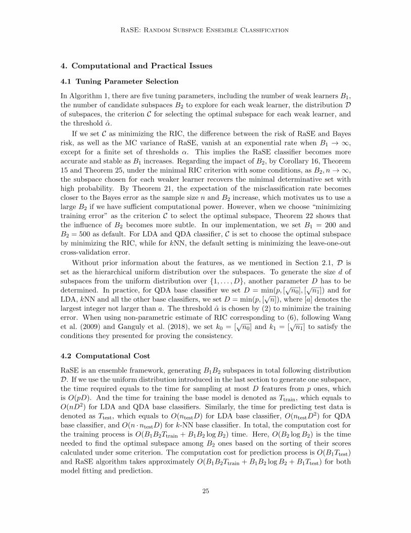
In Algorithm 1, there are five tuning parameters, including the number of weak learners B1,the number of candidate subspaces B2 to explore for each weak learner, the distribution Dof subspaces, the criterion C for selecting the optimal subspace for each weak learner, andthe threshold α.
If we set C as minimizing the RIC, the difference between the risk of RaSE and Bayesrisk, as well as the MC variance of RaSE, vanish at an exponential rate when B1 → ∞,except for a finite set of thresholds α. This implies the RaSE classifier becomes moreaccurate and stable as B1 increases. Regarding the impact of B2, by Corollary 16, Theorem15 and Theorem 25, under the minimal RIC criterion with some conditions, as B2, n→∞,the subspace chosen for each weaker learner recovers the minimal determinative set withhigh probability. By Theorem 21, the expectation of the misclassification rate becomescloser to the Bayes error as the sample size n and B2 increase, which motivates us to use alarge B2 if we have sufficient computational power. However, when we choose “minimizingtraining error” as the criterion C to select the optimal subspace, Theorem 22 shows thatthe influence of B2 becomes more subtle. In our implementation, we set B1 = 200 andB2 = 500 as default. For LDA and QDA classifier, C is set to choose the optimal subspaceby minimizing the RIC, while for kNN, the default setting is minimizing the leave-one-outcross-validation error.
Without prior information about the features, as we mentioned in Section 2.1, D isset as the hierarchical uniform distribution over the subspaces. To generate the size d ofsubspaces from the uniform distribution over 1, . . . , D, another parameter D has to bedetermined. In practice, for QDA base classifier we set D = min(p, [
√n0], [
√n1]) and for
LDA, kNN and all the other base classifiers, we set D = min(p, [√n]), where [a] denotes the
largest integer not larger than a. The threshold α is chosen by (2) to minimize the trainingerror. When using non-parametric estimate of RIC corresponding to (6), following Wanget al. (2009) and Ganguly et al. (2018), we set k0 = [
√n0] and k1 = [
√n1] to satisfy the
conditions they presented for proving the consistency.
4.2 Computational Cost
RaSE is an ensemble framework, generating B1B2 subspaces in total following distributionD. If we use the uniform distribution introduced in the last section to generate one subspace,the time required equals to the time for sampling at most D features from p ones, whichis O(pD). And the time for training the base model is denoted as Ttrain, which equals toO(nD2) for LDA and QDA base classifiers. Similarly, the time for predicting test data isdenoted as Ttest, which equals to O(ntestD) for LDA base classifier, O(ntestD
2) for QDAbase classifier, and O(n ·ntestD) for k-NN base classifier. In total, the computation cost forthe training process is O(B1B2Ttrain + B1B2 logB2) time. Here, O(B2 logB2) is the timeneeded to find the optimal subspace among B2 ones based on the sorting of their scorescalculated under some criterion. The computation cost for prediction process is O(B1Ttest)and RaSE algorithm takes approximately O(B1B2Ttrain + B1B2 logB2 + B1Ttest) for bothmodel fitting and prediction.
25
Tian and Feng
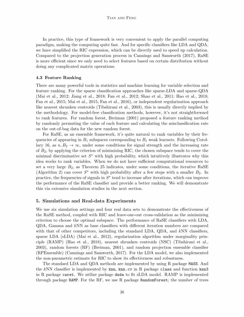
In practice, this type of framework is very convenient to apply the parallel computingparadigm, making the computing quite fast. And for specific classifiers like LDA and QDA,we have simplified the RIC expression, which can be directly used to speed up calculation.Compared to the projection generation process in Cannings and Samworth (2017), RaSEis more efficient since we only need to select features based on certain distribution withoutdoing any complicated matrix operations.
4.3 Feature Ranking
There are many powerful tools in statistics and machine learning for variable selection andfeature ranking. For the sparse classification approaches like sparse-LDA and sparse-QDA(Mai et al., 2012; Jiang et al., 2018; Fan et al., 2012; Shao et al., 2011; Hao et al., 2018;Fan et al., 2015; Mai et al., 2015; Fan et al., 2016), or independent regularization approachlike nearest shrunken centroids (Tibshirani et al., 2003), this is usually directly implied bythe methodology. For model-free classification methods, however, it’s not straightforwardto rank features. For random forest, Breiman (2001) proposed a feature ranking methodby randomly permuting the value of each feature and calculating the misclassification rateon the out-of-bag data for the new random forest.
For RaSE, as an ensemble framework, it’s quite natural to rank variables by their fre-quencies of appearing in B1 subspaces corresponding to B1 weak learners. Following Corol-lary 16, as n,B2 → ∞, under some conditions for signal strength and the increasing rateof B2, by applying the criterion of minimizing RIC, the chosen subspace tends to cover theminimal discriminative set S∗ with high probability, which intuitively illustrates why thisidea works to rank variables. When we do not have sufficient computational resources toset a very large B2, as Theorem 25 indicates, under some conditions, the iterative RaSE(Algorithm 2) can cover S∗ with high probability after a few steps with a smaller B2. Inpractice, the frequencies of signals in S∗ tend to increase after iterations, which can improvethe performance of the RaSE classifier and provide a better ranking. We will demonstratethis via extensive simulation studies in the next section.
5. Simulations and Real-data Experiments
We use six simulation settings and four real data sets to demonstrate the effectiveness ofthe RaSE method, coupled with RIC and leave-one-out cross-validation as the minimizingcriterion to choose the optimal subspace. The performance of RaSE classifiers with LDA,QDA, Gamma and kNN as base classifiers with different iteration numbers are comparedwith that of other competitors, including the standard LDA, QDA, and kNN classifiers,sparse LDA (sLDA) (Mai et al., 2012), regularization algorithm under marginality prin-ciple (RAMP) (Hao et al., 2018), nearest shrunken centroids (NSC) (Tibshirani et al.,2003), random forests (RF) (Breiman, 2001), and random projection ensemble classifier(RPEnsemble) (Cannings and Samworth, 2017). For the LDA model, we also implementedthe non-parametric estimate for RIC to show its effectiveness and robustness.
The standard LDA and QDA methods are implemented by using R package MASS. Andthe kNN classifier is implemented by knn, knn.cv in R package class and function knn3
in R package caret. We utilize package dsda to fit sLDA model. RAMP is implementedthrough package RAMP. For the RF, we use R package RandomForest; the number of trees
26

RaSE: Random Subspace Ensemble Classification
are set as 500 (as default) and [√p] variables are randomly selected when training each tree
(as default). And the NSC model is fitted by calling function pamr.train in package pamr.RPEnsemble is implemented by R package RPEnsemble. To obtain the MLE of parametersin the Gamma distribution, the Newton’s method is applied via function nlm in packagestats and the initial point is chosen to be the moment estimator. To get the non-parametricestimate of KL divergence and RIC, we call function KL.divergence in package FNN.
When fitting the standard kNN classifier, and the kNN base classifier in RPEnsembleand RaSE method, the number of neighbors k is chosen from 3, 5, 7, 9, 11 via leave-one-outcross-validation, following Cannings and Samworth (2017). For RAMP, the response type isset as “binomial”, for which the logistic regression with interaction effects is considered. InsLDA, the penalty parameter λ is chosen to minimize cross-validation error. In RPEnsemblemethod, LDA, QDA, kNN, are set as base classifiers with default parameters, and thenumber of weak learner B1 = 500 and the number of projection candidates for each weaklearner B2 = 50 and the dimension of projected space d = 5. The projection generationmethod is set to be “Haar”. The criterion of choosing optimal projection is set to minimizetraining error for LDA and QDA and minimize leave-one-out cross-validation error for kNN.For the RaSE method, for LDA, QDA, and independent Gamma classifier (to be illustratedlater in Section 5.1.2), the criterion is set to be minimizing RIC, and for k-NN, the strategyof minimizing leave-one-out cross-validation error is applied. Other parameter settings inRaSE are the same as in the last section. For simulations, the number of iterations T inAlgorithm 2 is set to be 0, 1, 2, while for real-data experiments, we only consider RaSEmethods with 0 or 1 iteration. We write the iteration number on the subscript, and if it iszero, the subscript will be omitted. For example, RaSE1-LDA represents the RaSE classifierwith T = 1 iteration and LDA base classifier. In addition, we use LDAn to denote the LDAbase classifier with the non-parametric estimate of RIC.
For all experiments, 200 replicates are considered, and the average test errors (percent-age) are calculated based on them. The standard deviation of the test errors over 200replicates is also calculated for each approach and written on the subscript. The approachwith minimal test error for each setting is highlighted in bold, and methods that achievetest error within one standard deviation of the best one are highlighted in italics. Also,for all simulations and the madelon data set, the average selected percentage of featuresin B1 subspaces for the largest sample size setting in the RaSE method in 200 replicatesare presented, which provides a natural way for feature ranking. For the average selectedpercentage in the case of the smallest sample size, refer to Appendix A. To highlight thedifferent behaviors of signals and noises, we present the average selected percentages of allnoise features as a box-plot marked with “N”.
The RaSE classifier competes favorably with existing classification methods. Its mis-classification rate is the lowest in 27 out of 30 (simulation and real-data) settings and withinone standard deviation of the lowest in the remaining four settings.
5.1 Simulations
For the simulated data, model 1 follows model 1 in Mai et al. (2012), which is a sparseLDA-adapted setting. In model 2, for each class, a Gamma distribution with independentcomponents is used. Model 3 follows from the setting of model 3 in Fan et al. (2015), which is
27

Tian and Feng
a QDA-adapted model. The marginal distribution for two classes is set to be π0 = π1 = 0.5for the first three simulation models. Model 4 is motivated by the kNN algorithm, andthe data generation process will be introduced below. To test the robustness of RaSE, twonon-sparse settings, model 1’ and 4’ are investigated as well, where model 1’ has decayingsignals in the LDA model while model 4’ inherits from model 4 by increasing the numberof signals to 30 with the signal strength decreased.
For simulations, we consider the “signal” model as a benchmark. These models use thecorrect model on the minimal discriminative set S∗, mimicking the behavior of the Bayesclassifier when S∗ is sparse.
5.1.1 Models 1 and 1’ (LDA)
First we consider a sparse LDA setting (model 1). Let x|y = r ∼ N(µ(r),Σ), r = 0, 1,where Σ = (Σij)p×p = (0.5|i−j|)p×p,µ
(0) = 0p×1,µ(1) = Σ × 0.556(3, 1.5, 0, 0, 2,01×(p−5))
T .Here p = 400, and the training sample size n ∈ 200, 400, 1000. Test data of size 1000 isindependently generated from the same model.
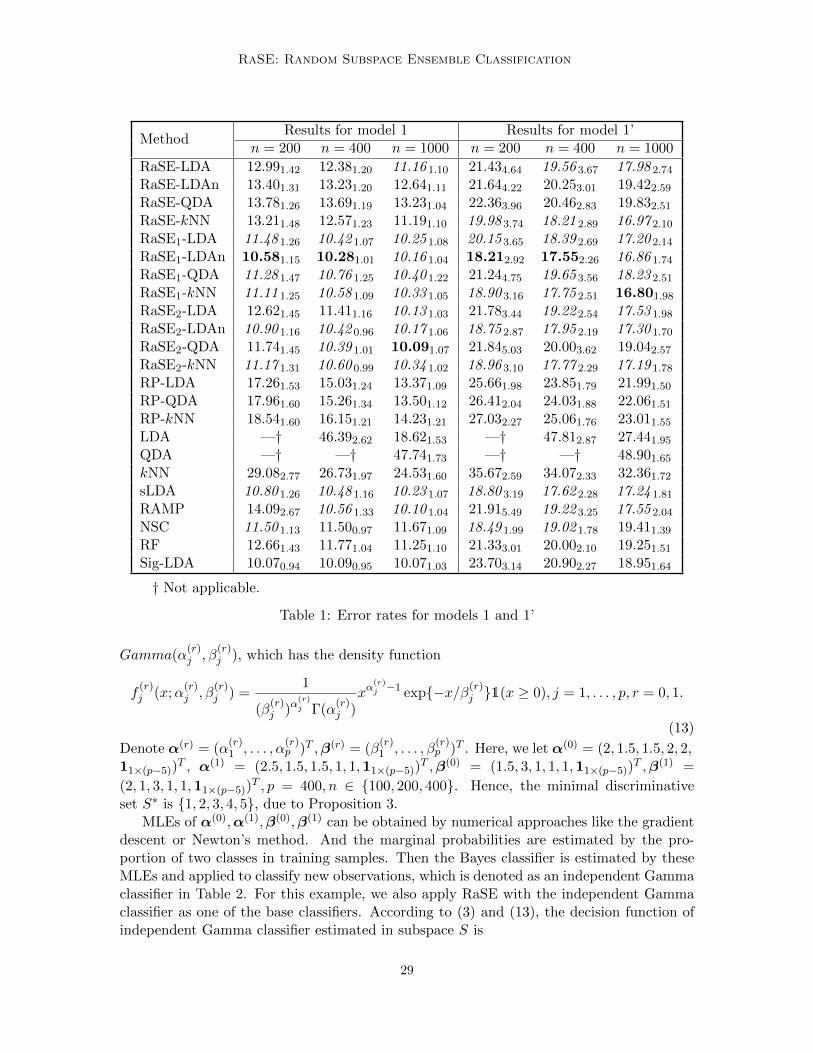
As analyzed in Example 1, feature subset 1, 2, 5 is the minimal discriminative set S∗.On the left panel of Table 1, the performance of various methods on model 1 for differentsample sizes are presented. As we could see, RaSE1-LDAn performs the best when thesample size n = 200 and 400. sLDA achieves similar performances to the best classifiers foreach setting, and RaSE2-QDA ranks the top when n = 1000. Also, since this model is verysparse, the default value of B2 cannot guarantee that the minimal discriminative set can beselected. Therefore the iterative version of RaSE improves the performance of RaSE a lot.And NSC also achieves a comparably small misclassification rate when n = 200.
In Figure 1, the average selected percentages of 400 features in 200 replicates whenn = 1000 are presented. Note that after two iterations, the three signals can be captured byalmost all B1 = 200 subspaces for all three base classifiers, and all noises are rarely selectedacross B1 subspaces except when the non-parametric estimate of RIC is applied.
Next, we consider a non-sparse LDA model (model 1’). Let µ(1) = Σ·(0.9, 0.92, . . . , 0.950,01×(p−50))
T and keep other parameters the same as above. Now S∗ contains the first 50features. Under this non-sparse setting, as the right panel of Table 1 shows, althoughmost methods obtain similar error rates, RaSE1-LDAn achieves the best performance whenn = 200 and 400. RaSE1-kNN performs the best when n = 1000. From the table, it can beseen that despite the non-sparse design, the iterations can still improve the performance ofRaSE.
An interesting phenomenon is observed from Figure 2, which exhibits the average se-lected percentages for model 1’. Note that the selected percentages are decaying as the signalstrength decreases except for the first feature. One possible reason is that the marginal dis-criminative powers of feature 2 and 3 are the strongest among all features due to the specificcorrelation structure in our setting.
5.1.2 Model 2 (Gamma distribution)
In this model we investigate the Gamma distribution with independent features, which israrely studied in the literature. x|y = r at j-th coordinate follows Gamma distribution
28
RaSE: Random Subspace Ensemble Classification
MethodResults for model 1 Results for model 1’
n = 200 n = 400 n = 1000 n = 200 n = 400 n = 1000
RaSE-LDA 12.991.42 12.381.20 11.16 1.10 21.434.64 19.56 3.67 17.98 2.74
RaSE-LDAn 13.401.31 13.231.20 12.641.11 21.644.22 20.253.01 19.422.59
RaSE-QDA 13.781.26 13.691.19 13.231.04 22.363.96 20.462.83 19.832.51
RaSE-kNN 13.211.48 12.571.23 11.191.10 19.98 3.74 18.21 2.89 16.97 2.10
RaSE1-LDA 11.48 1.26 10.42 1.07 10.25 1.08 20.15 3.65 18.39 2.69 17.20 2.14
RaSE1-LDAn 10.581.15 10.281.01 10.16 1.04 18.212.92 17.552.26 16.86 1.74
RaSE1-QDA 11.28 1.47 10.76 1.25 10.40 1.22 21.244.75 19.65 3.56 18.23 2.51
RaSE1-kNN 11.11 1.25 10.58 1.09 10.33 1.05 18.90 3.16 17.75 2.51 16.801.98
RaSE2-LDA 12.621.45 11.411.16 10.13 1.03 21.783.44 19.22 2.54 17.53 1.98
RaSE2-LDAn 10.90 1.16 10.42 0.96 10.17 1.06 18.75 2.87 17.95 2.19 17.30 1.70
RaSE2-QDA 11.741.45 10.39 1.01 10.091.07 21.845.03 20.003.62 19.042.57
RaSE2-kNN 11.17 1.31 10.60 0.99 10.34 1.02 18.96 3.10 17.77 2.29 17.19 1.78
RP-LDA 17.261.53 15.031.24 13.371.09 25.661.98 23.851.79 21.991.50
RP-QDA 17.961.60 15.261.34 13.501.12 26.412.04 24.031.88 22.061.51
RP-kNN 18.541.60 16.151.21 14.231.21 27.032.27 25.061.76 23.011.55
LDA —† 46.392.62 18.621.53 —† 47.812.87 27.441.95
QDA —† —† 47.741.73 —† —† 48.901.65
kNN 29.082.77 26.731.97 24.531.60 35.672.59 34.072.33 32.361.72
sLDA 10.80 1.26 10.48 1.16 10.23 1.07 18.80 3.19 17.62 2.28 17.24 1.81
RAMP 14.092.67 10.56 1.33 10.10 1.04 21.915.49 19.22 3.25 17.55 2.04
NSC 11.50 1.13 11.500.97 11.671.09 18.49 1.99 19.02 1.78 19.411.39
RF 12.661.43 11.771.04 11.251.10 21.333.01 20.002.10 19.251.51
Sig-LDA 10.070.94 10.090.95 10.071.03 23.703.14 20.902.27 18.951.64
† Not applicable.
Table 1: Error rates for models 1 and 1’
Gamma(α(r)j , β
(r)j ), which has the density function
f(r)j (x;α
(r)j , β
(r)j ) =
1
(β(r)j )α
(r)j Γ(α
(r)j )
xα(r)j −1 exp−x/β(r)
j 1(x ≥ 0), j = 1, . . . , p, r = 0, 1.
(13)
Denote α(r) = (α(r)1 , . . . , α
(r)p )T ,β(r) = (β
(r)1 , . . . , β
(r)p )T . Here, we let α(0) = (2, 1.5, 1.5, 2, 2,
11×(p−5))T , α(1) = (2.5, 1.5, 1.5, 1, 1,11×(p−5))
T ,β(0) = (1.5, 3, 1, 1, 1,11×(p−5))T ,β(1) =
(2, 1, 3, 1, 1,11×(p−5))T , p = 400, n ∈ 100, 200, 400. Hence, the minimal discriminative
set S∗ is 1, 2, 3, 4, 5, due to Proposition 3.MLEs of α(0),α(1),β(0),β(1) can be obtained by numerical approaches like the gradient
descent or Newton’s method. And the marginal probabilities are estimated by the pro-portion of two classes in training samples. Then the Bayes classifier is estimated by theseMLEs and applied to classify new observations, which is denoted as an independent Gammaclassifier in Table 2. For this example, we also apply RaSE with the independent Gammaclassifier as one of the base classifiers. According to (3) and (13), the decision function ofindependent Gamma classifier estimated in subspace S is
29

Tian and Feng
0
25
50
75
100
1 2 5 Nfeature
sele
cted
per
cent
age
RaSE−LDA
0
25
50
75
100
1 2 5 Nfeature
sele
cted
per
cent
age
RaSE1−LDA
0
25
50
75
100
1 2 5 Nfeature
sele
cted
per
cent
age
RaSE2−LDA
0
25
50
75
100
1 2 5 Nfeature
sele
cted
per
cent
age
RaSE−LDAn
0
25
50
75
100
1 2 5 Nfeature
sele
cted
per
cent
age
RaSE1−LDAn
0
25
50
75
100
1 2 5 Nfeature
sele
cted
per
cent
age
RaSE2−LDAn
0
20
40
60
80
1 2 5 Nfeature
sele
cted
per
cent
age
RaSE−QDA
0
25
50
75
100
1 2 5 Nfeature
sele
cted
per
cent
age
RaSE1−QDA
0
25
50
75
100
1 2 5 Nfeature
sele
cted
per
cent
age
RaSE2−QDA
0
25
50
75
100
1 2 5 Nfeature
sele
cted
per
cent
age
RaSE−kNN
0
25
50
75
100
1 2 5 Nfeature
sele
cted
per
cent
age
RaSE1−kNN
0
25
50
75
100
1 2 5 Nfeature
sele
cted
per
cent
age
RaSE2−kNN
Figure 1: Average selected percentages of features for model 1 in 200 replicates when n =1000
CS−Gamman (x) = 1
π1
π0·∏j∈S
f(1)j (xj ; α
(1)j , β
(1)j )
f(0)j (xj ; α
(0)j , β
(0)j )
> 0.5
,
where π1, π0, α(1)j , α
(0)j , β
(1)j , β
(0)j are corresponding MLEs.
This is also a very sparse model. Therefore the iteration process can improve the RaSEmethod with a lower misclassification rate. The left panel of Table 2 shows us the perfor-mance of various methods on this model. It demonstrates that RaSE1-Gamma performs
30
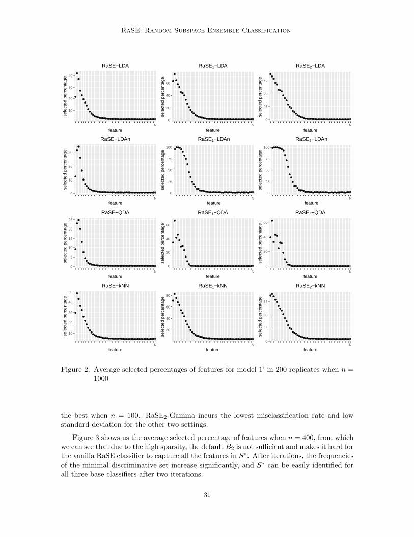
RaSE: Random Subspace Ensemble Classification
10
20
30
40
Nfeature
sele
cted
per
cent
age
RaSE−LDA
0
20
40
60
Nfeature
sele
cted
per
cent
age
RaSE1−LDA
0
25
50
75
Nfeature
sele
cted
per
cent
age
RaSE2−LDA
0
10
20
30
Nfeature
sele
cted
per
cent
age
RaSE−LDAn
0
25
50
75
100
Nfeature
sele
cted
per
cent
age
RaSE1−LDAn
0
25
50
75
100
Nfeature
sele
cted
per
cent
age
RaSE2−LDAn
0
5
10
15
20
25
Nfeature
sele
cted
per
cent
age
RaSE−QDA
0
20
40
60
Nfeature
sele
cted
per
cent
age
RaSE1−QDA
0
20
40
60
Nfeature
sele
cted
per
cent
age
RaSE2−QDA
10
20
30
40
50
Nfeature
sele
cted
per
cent
age
RaSE−kNN
20
40
60
80
Nfeature
sele
cted
per
cent
age
RaSE1−kNN
0
25
50
75
Nfeature
sele
cted
per
cent
age
RaSE2−kNN
Figure 2: Average selected percentages of features for model 1’ in 200 replicates when n =1000
the best when n = 100. RaSE2-Gamma incurs the lowest misclassification rate and lowstandard deviation for the other two settings.
Figure 3 shows us the average selected percentage of features when n = 400, from whichwe can see that due to the high sparsity, the default B2 is not sufficient and makes it hard forthe vanilla RaSE classifier to capture all the features in S∗. After iterations, the frequenciesof the minimal discriminative set increase significantly, and S∗ can be easily identified forall three base classifiers after two iterations.
31
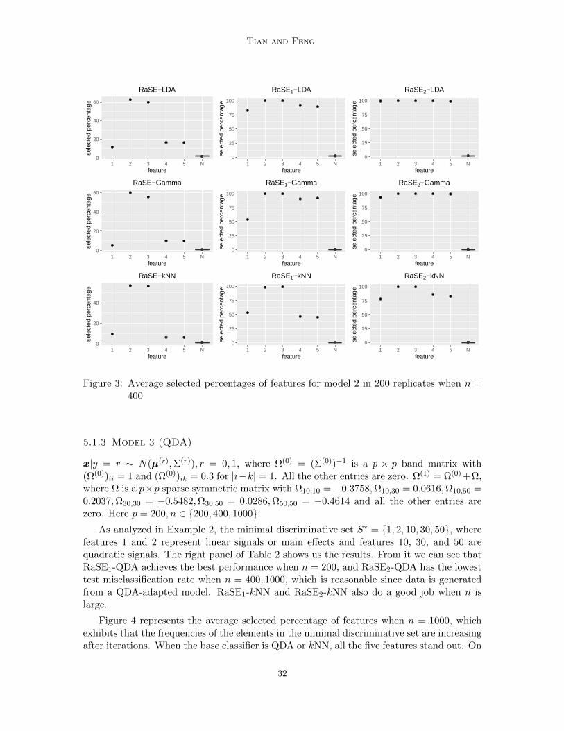
Tian and Feng
0
20
40
60
1 2 3 4 5 Nfeature
sele
cted
per
cent
age
RaSE−LDA
0
25
50
75
100
1 2 3 4 5 Nfeature
sele
cted
per
cent
age
RaSE1−LDA
0
25
50
75
100
1 2 3 4 5 Nfeature
sele
cted
per
cent
age
RaSE2−LDA
0
20
40
60
1 2 3 4 5 Nfeature
sele
cted
per
cent
age
RaSE−Gamma
0
25
50
75
100
1 2 3 4 5 Nfeature
sele
cted
per
cent
age
RaSE1−Gamma
0
25
50
75
100
1 2 3 4 5 Nfeature
sele
cted
per
cent
age
RaSE2−Gamma
0
20
40
1 2 3 4 5 Nfeature
sele
cted
per
cent
age
RaSE−kNN
0
25
50
75
100
1 2 3 4 5 Nfeature
sele
cted
per
cent
age
RaSE1−kNN
0
25
50
75
100
1 2 3 4 5 Nfeature
sele
cted
per
cent
age
RaSE2−kNN
Figure 3: Average selected percentages of features for model 2 in 200 replicates when n =400
5.1.3 Model 3 (QDA)
x|y = r ∼ N(µ(r),Σ(r)), r = 0, 1, where Ω(0) = (Σ(0))−1 is a p × p band matrix with(Ω(0))ii = 1 and (Ω(0))ik = 0.3 for |i−k| = 1. All the other entries are zero. Ω(1) = Ω(0) +Ω,where Ω is a p×p sparse symmetric matrix with Ω10,10 = −0.3758,Ω10,30 = 0.0616,Ω10,50 =0.2037,Ω30,30 = −0.5482,Ω30,50 = 0.0286,Ω50,50 = −0.4614 and all the other entries arezero. Here p = 200, n ∈ 200, 400, 1000.
As analyzed in Example 2, the minimal discriminative set S∗ = 1, 2, 10, 30, 50, wherefeatures 1 and 2 represent linear signals or main effects and features 10, 30, and 50 arequadratic signals. The right panel of Table 2 shows us the results. From it we can see thatRaSE1-QDA achieves the best performance when n = 200, and RaSE2-QDA has the lowesttest misclassification rate when n = 400, 1000, which is reasonable since data is generatedfrom a QDA-adapted model. RaSE1-kNN and RaSE2-kNN also do a good job when n islarge.
Figure 4 represents the average selected percentage of features when n = 1000, whichexhibits that the frequencies of the elements in the minimal discriminative set are increasingafter iterations. When the base classifier is QDA or kNN, all the five features stand out. On
32

RaSE: Random Subspace Ensemble Classification
the other hand, RaSE, with the LDA base classifier, only captures the two linear signals,which is expected since LDA does not consider the quadratic terms.
Method3 Results for model 2 Results for model 3n = 100 n = 200 n = 400 n = 200 n = 400 n = 1000
RaSE-LDA 21.513.42 18.522.75 17.432.00 37.303.17 36.111.97 35.671.73
RaSE-Gamma/QDA 23.573.65 21.413.17 20.292.43 32.522.90 30.442.60 29.001.97
RaSE-kNN 22.833.09 21.073.07 20.472.57 31.103.23 27.832.41 25.221.56
RaSE1-LDA 19.012.83 15.141.75 13.551.20 36.092.87 32.821.74 32.681.49
RaSE1-Gamma/QDA 15.052.31 13.02 1.51 12.50 1.18 26.832.47 25.07 1.89 23.53 1.50
RaSE1-kNN 19.842.90 16.641.86 15.331.39 28.76 2.60 25.88 1.98 24.18 1.47
RaSE2-LDA 20.883.03 16.922.05 13.661.14 38.092.48 33.691.83 32.711.55
RaSE2-Gamma/QDA 16.27 2.22 12.641.31 11.831.02 26.99 2.68 24.871.99 23.111.60
RaSE2-kNN 22.393.13 17.402.27 14.591.44 28.73 2.56 25.46 1.82 23.76 1.54
RP-LDA 38.891.96 35.001.97 30.891.76 44.901.86 42.821.76 40.381.74
RP-QDA 43.623.62 37.622.35 33.022.14 43.022.07 39.871.88 36.381.78
RP-kNN 41.482.26 38.902.06 36.691.85 44.321.81 42.461.58 40.802.12
LDA —† —† 47.502.35 49.031.94 42.881.82 38.681.70
QDA 32.062.40 26.221.80 21.561.44 —† —† 45.131.58
kNN 45.482.24 44.682.14 44.072.00 45.671.78 44.632.02 43.431.63
sLDA 22.263.52 18.642.12 15.341.55 36.413.15 33.872.01 32.991.52
RAMP 20.643.81 16.722.25 13.311.21 36.945.87 32.651.89 32.421.78
NSC 26.006.49 19.924.31 16.872.69 41.144.49 38.243.85 35.132.20
RF 24.975.74 18.022.77 15.261.47 37.342.91 31.612.19 27.421.60
Sig-Gamma/QDA 12.651.12 12.121.12 11.760.97 23.621.47 22.721.40 22.161.31
† Not applicable.
Table 2: Error rates for models 2 and 3
5.1.4 Models 4 and 4’ (kNN)
As in the LDA models, we first study a sparse setting (model 4) with the data generatingprocess motivated by the kNN classifier. First, 10 initial points z1, . . . ,z10 are generatedi.i.d. from N(0p×1, Ip), five of which are labeled as 0 and the other five are labeled as1. Then each time one of z1, . . . ,z10 is randomly selected (suppose zki) and we thengenerate xi ∼ N((zTki,S∗ ,01×(p−5))
T , 0.52Ip). Here the minimal discriminative set is S∗ =1, 2, 3, 4, 5, p = 200, and n ∈ 200, 400, 1000. The results are presented in Table 3 andthe average selected percentages of features in B1 = 200 subspaces are presented in Figure5.
From the left panel of Table 3, it can be seen that the performance of RaSE2-kNN issurprising. It outperforms all the other methods, and the difference between its misclassi-fication rate and others is very prominent. Note that in this case, the Sig-kNN classifieris calculated by applying kNN on only the first five features and also uses leave-one-out
3. To save space, for the rows involving “Gamma/QDA”, it represents the independent Gamma classifierin model 2 and the QDA in model 3.
33

Tian and Feng
0
25
50
75
1 2 10 30 50 Nfeature
sele
cted
per
cent
age
RaSE−LDA
0
25
50
75
100
1 2 10 30 50 Nfeature
sele
cted
per
cent
age
RaSE1−LDA
0
25
50
75
100
1 2 10 30 50 Nfeature
sele
cted
per
cent
age
RaSE2−LDA
0
10
20
30
40
1 2 10 30 50 Nfeature
sele
cted
per
cent
age
RaSE−QDA
0
25
50
75
100
1 2 10 30 50 Nfeature
sele
cted
per
cent
age
RaSE1−QDA
0
25
50
75
100
1 2 10 30 50 Nfeature
sele
cted
per
cent
age
RaSE2−QDA
20
40
60
1 2 10 30 50 Nfeature
sele
cted
per
cent
age
RaSE−kNN
0
25
50
75
1 2 10 30 50 Nfeature
sele
cted
per
cent
age
RaSE1−kNN
0
25
50
75
100
1 2 10 30 50 Nfeature
sele
cted
per
cent
age
RaSE2−kNN
Figure 4: Average selected percentages of features for model 3 in 200 replicates when n =1000
cross-validation to choose k from 3, 5, 7, 9, 11. Note that it is not the optimal classifierdue to the lack of a true model, which explains why RaSE2-kNN can even achieve a betterperformance when n = 400, 1000.
Figure 5 shows that RaSE, based on all the three base classifiers, can capture featuresin the minimal discriminative set.
Now, we study a non-sparse setting (model 4’), where the number of signals are in-creased to 30 and each xi ∼ N((zTki,S∗ ,01×(p−30))
T , 2Ip). The other parameters and thedata generation mechanism are the same as model 4. From the right panel of Table 3, weobserve that RaSE2-kNN still achieves the best performance, and the iterations improve theperformance of RaSE classifiers under this non-sparse setting. In addition, Figure 6 showsthat RaSE can capture the signals while the noises keep a low selected percentage, whichagain verifies the robustness of RaSE.
34
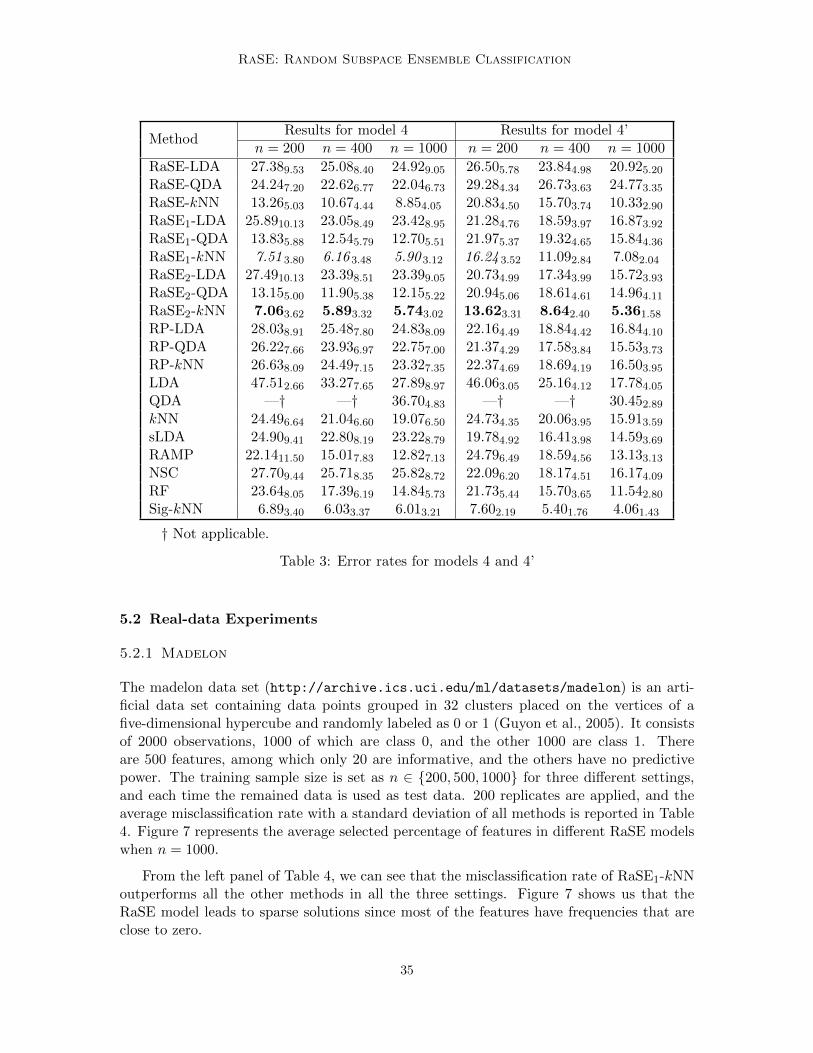
RaSE: Random Subspace Ensemble Classification
MethodResults for model 4 Results for model 4’
n = 200 n = 400 n = 1000 n = 200 n = 400 n = 1000
RaSE-LDA 27.389.53 25.088.40 24.929.05 26.505.78 23.844.98 20.925.20
RaSE-QDA 24.247.20 22.626.77 22.046.73 29.284.34 26.733.63 24.773.35
RaSE-kNN 13.265.03 10.674.44 8.854.05 20.834.50 15.703.74 10.332.90
RaSE1-LDA 25.8910.13 23.058.49 23.428.95 21.284.76 18.593.97 16.873.92
RaSE1-QDA 13.835.88 12.545.79 12.705.51 21.975.37 19.324.65 15.844.36
RaSE1-kNN 7.51 3.80 6.16 3.48 5.90 3.12 16.24 3.52 11.092.84 7.082.04
RaSE2-LDA 27.4910.13 23.398.51 23.399.05 20.734.99 17.343.99 15.723.93
RaSE2-QDA 13.155.00 11.905.38 12.155.22 20.945.06 18.614.61 14.964.11
RaSE2-kNN 7.063.62 5.893.32 5.743.02 13.623.31 8.642.40 5.361.58
RP-LDA 28.038.91 25.487.80 24.838.09 22.164.49 18.844.42 16.844.10
RP-QDA 26.227.66 23.936.97 22.757.00 21.374.29 17.583.84 15.533.73
RP-kNN 26.638.09 24.497.15 23.327.35 22.374.69 18.694.19 16.503.95
LDA 47.512.66 33.277.65 27.898.97 46.063.05 25.164.12 17.784.05
QDA —† —† 36.704.83 —† —† 30.452.89
kNN 24.496.64 21.046.60 19.076.50 24.734.35 20.063.95 15.913.59
sLDA 24.909.41 22.808.19 23.228.79 19.784.92 16.413.98 14.593.69
RAMP 22.1411.50 15.017.83 12.827.13 24.796.49 18.594.56 13.133.13
NSC 27.709.44 25.718.35 25.828.72 22.096.20 18.174.51 16.174.09
RF 23.648.05 17.396.19 14.845.73 21.735.44 15.703.65 11.542.80
Sig-kNN 6.893.40 6.033.37 6.013.21 7.602.19 5.401.76 4.061.43
† Not applicable.
Table 3: Error rates for models 4 and 4’
5.2 Real-data Experiments
5.2.1 Madelon
The madelon data set (http://archive.ics.uci.edu/ml/datasets/madelon) is an arti-ficial data set containing data points grouped in 32 clusters placed on the vertices of afive-dimensional hypercube and randomly labeled as 0 or 1 (Guyon et al., 2005). It consistsof 2000 observations, 1000 of which are class 0, and the other 1000 are class 1. Thereare 500 features, among which only 20 are informative, and the others have no predictivepower. The training sample size is set as n ∈ 200, 500, 1000 for three different settings,and each time the remained data is used as test data. 200 replicates are applied, and theaverage misclassification rate with a standard deviation of all methods is reported in Table4. Figure 7 represents the average selected percentage of features in different RaSE modelswhen n = 1000.
From the left panel of Table 4, we can see that the misclassification rate of RaSE1-kNNoutperforms all the other methods in all the three settings. Figure 7 shows us that theRaSE model leads to sparse solutions since most of the features have frequencies that areclose to zero.
35
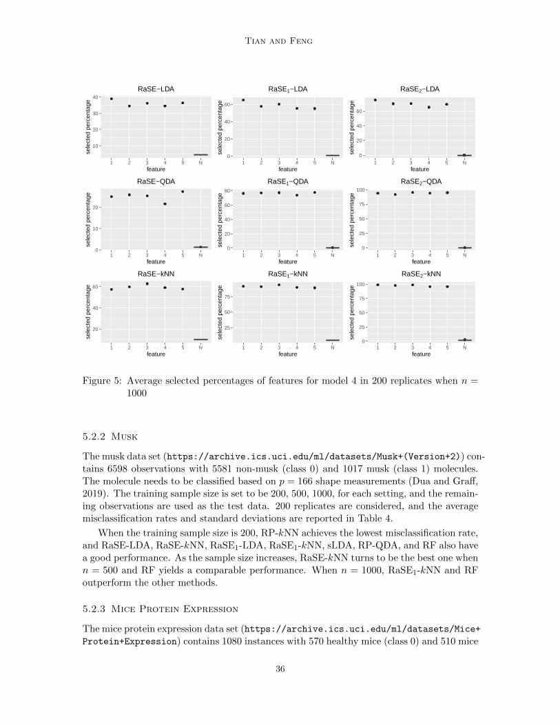
Tian and Feng
10
20
30
40
1 2 3 4 5 Nfeature
sele
cted
per
cent
age
RaSE−LDA
0
20
40
60
1 2 3 4 5 Nfeature
sele
cted
per
cent
age
RaSE1−LDA
0
20
40
60
1 2 3 4 5 Nfeature
sele
cted
per
cent
age
RaSE2−LDA
0
10
20
1 2 3 4 5 Nfeature
sele
cted
per
cent
age
RaSE−QDA
0
20
40
60
80
1 2 3 4 5 Nfeature
sele
cted
per
cent
age
RaSE1−QDA
0
25
50
75
100
1 2 3 4 5 Nfeature
sele
cted
per
cent
age
RaSE2−QDA
20
40
60
1 2 3 4 5 Nfeature
sele
cted
per
cent
age
RaSE−kNN
25
50
75
1 2 3 4 5 Nfeature
sele
cted
per
cent
age
RaSE1−kNN
0
25
50
75
100
1 2 3 4 5 Nfeature
sele
cted
per
cent
age
RaSE2−kNN
Figure 5: Average selected percentages of features for model 4 in 200 replicates when n =1000
5.2.2 Musk
The musk data set (https://archive.ics.uci.edu/ml/datasets/Musk+(Version+2)) con-tains 6598 observations with 5581 non-musk (class 0) and 1017 musk (class 1) molecules.The molecule needs to be classified based on p = 166 shape measurements (Dua and Graff,2019). The training sample size is set to be 200, 500, 1000, for each setting, and the remain-ing observations are used as the test data. 200 replicates are considered, and the averagemisclassification rates and standard deviations are reported in Table 4.
When the training sample size is 200, RP-kNN achieves the lowest misclassification rate,and RaSE-LDA, RaSE-kNN, RaSE1-LDA, RaSE1-kNN, sLDA, RP-QDA, and RF also havea good performance. As the sample size increases, RaSE-kNN turns to be the best one whenn = 500 and RF yields a comparable performance. When n = 1000, RaSE1-kNN and RFoutperform the other methods.
5.2.3 Mice Protein Expression
The mice protein expression data set (https://archive.ics.uci.edu/ml/datasets/Mice+Protein+Expression) contains 1080 instances with 570 healthy mice (class 0) and 510 mice
36

RaSE: Random Subspace Ensemble Classification
5
10
15
Nfeature
sele
cted
per
cent
age
RaSE−LDA
10
20
30
Nfeature
sele
cted
per
cent
age
RaSE1−LDA
10
20
30
40
Nfeature
sele
cted
per
cent
age
RaSE2−LDA
2
4
6
Nfeature
sele
cted
per
cent
age
RaSE−QDA
0
10
20
Nfeature
sele
cted
per
cent
age
RaSE1−QDA
0
10
20
30
Nfeature
sele
cted
per
cent
age
RaSE2−QDA
10
15
20
25
Nfeature
sele
cted
per
cent
age
RaSE−kNN
10
20
30
40
Nfeature
sele
cted
per
cent
age
RaSE1−kNN
10
20
30
40
50
Nfeature
sele
cted
per
cent
age
RaSE2−kNN
Figure 6: Average selected percentages of features for model 4 in 200 replicates when n =1000
with Down’s syndrome (class 1). There are 77 features representing the expression of 77 dif-ferent proteins (Higuera et al., 2015). Training samples of size 200, 500, 800 are considered,and the remaining observations are set as the test data.
The average of test misclassification rates and the standard deviations of 200 replicatesare calculated with results reported in Table 5. When n = 200, sLDA achieves the lowesterror among all approaches, and RaSE-kNN achieves a similar performance. As the samplesize increases to 500 and 800, the average misclassification rate of RaSE-kNN and RaSE1-kNN decrease significantly, and they become the best classifier when n = 500 and 800,respectively. When n = 800, RP-kNN and RF also have a similar performance.
5.2.4 Hand-written Digits Recognition
The hand-written digits recognition data set (https://archive.ics.uci.edu/ml/datasets/Multiple+Features) consists of features of hand-written numerals (0-9) extracted from acollection of Dutch utility maps (Dua and Graff, 2019). Here we use the mfeat-fou data set,which records 76 Fourier coefficients of the character shapes. We extract the observationscorresponding to number 7 (class 0) and 9 (class 1) from the original data. There are 400observations, 200 of which belong to class 0, and the remaining 200 belong to class 1. The
37
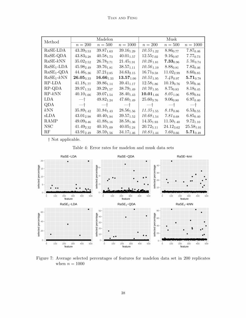
Tian and Feng
MethodMadelon Musk
n = 200 n = 500 n = 1000 n = 200 n = 500 n = 1000
RaSE-LDA 43.393.53 39.871.63 39.161.29 10.55 1.22 8.860.77 7.870.46
RaSE-QDA 43.833.28 40.581.73 40.011.57 12.557.02 9.160.97 7.770.73
RaSE-kNN 35.022.52 26.782.71 21.451.91 10.26 1.81 7.330.96 5.76 0.74
RaSE1-LDA 45.982.49 39.761.81 38.571.11 10.56 1.19 8.880.81 7.820.46
RaSE1-QDA 44.465.36 37.212.85 34.632.15 16.719.58 11.022.99 8.600.85
RaSE1-kNN 26.053.33 16.661.33 13.571.00 10.52 1.95 7.49 0.97 5.710.78
RP-LDA 41.181.77 39.861.14 39.411.17 12.581.86 10.190.76 9.500.46
RP-QDA 39.971.53 39.291.57 38.791.49 10.70 1.95 8.750.83 8.180.45
RP-kNN 40.101.66 39.071.54 38.401.43 10.011.66 8.05 1.06 6.890.84
LDA —† 49.821.24 47.601.49 25.603.76 9.060.80 6.970.40
QDA —† —† —† —† —† —†kNN 35.891.42 31.841.43 28.561.56 11.35 1.55 8.19 0.86 6.530.55
sLDA 43.012.98 40.401.94 39.571.52 10.68 1.54 7.81 0.68 6.850.40
RAMP 49.093.46 41.885.16 38.581.36 14.351.93 11.501.40 9.721.10
NSC 41.492.32 40.101.09 40.051.24 20.725.11 24.123.62 25.581.01
RF 43.912.49 38.591.56 34.171.46 10.83 1.44 7.60 0.66 5.710.48
† Not applicable.
Table 4: Error rates for madelon and musk data sets
0
5
10
15
20
0 100 200 300 400 500feature
sele
cted
per
cent
age
RaSE−LDA
0
2
4
6
0 100 200 300 400 500feature
sele
cted
per
cent
age
RaSE−QDA
10
20
30
40
0 100 200 300 400 500feature
sele
cted
per
cent
age
RaSE−knn
0
20
40
60
0 100 200 300 400 500feature
sele
cted
per
cent
age
RaSE1−LDA
0
10
20
30
40
50
0 100 200 300 400 500feature
sele
cted
per
cent
age
RaSE1−QDA
0
20
40
60
80
0 100 200 300 400 500feature
sele
cted
per
cent
age
RaSE1−kNN
Figure 7: Average selected percentages of features for madelon data set in 200 replicateswhen n = 1000
38
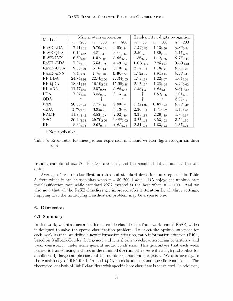
RaSE: Random Subspace Ensemble Classification
MethodMice protein expression Hand-written digits recognition
n = 200 n = 500 n = 800 n = 50 n = 100 n = 200
RaSE-LDA 7.411.14 5.700.93 4.651.24 1.56 0.85 1.130.59 0.80 0.54
RaSE-QDA 9.142.58 4.811.17 3.441.23 2.501.47 1.890.91 1.470.96
RaSE-kNN 6.801.88 1.550.88 0.62 0.55 1.860.96 1.120.66 0.75 0.45
RaSE1-LDA 7.241.10 5.531.02 4.491.23 1.060.63 0.70 0.35 0.530.40
RaSE1-QDA 9.382.21 5.161.16 3.401.16 2.181.66 1.180.71 0.85 0.61
RaSE1-kNN 7.432.00 1.70 0.87 0.600.56 1.720.95 1.02 0.62 0.60 0.44
RP-LDA 24.842.91 22.792.50 22.342.55 1.751.29 1.220.67 1.040.61
RP-QDA 18.312.57 16.192.08 15.662.38 2.121.67 1.280.94 0.92 0.62
RP-kNN 11.772.54 2.570.89 0.92 0.68 1.68 1.34 1.03 0.60 0.84 0.59
LDA 7.071.37 3.880.85 3.131.08 —† 1.820.96 1.010.56
QDA —† —† —† —† —† 3.252.32
kNN 20.532.47 7.751.44 2.801.21 1.42 1.32 0.670.41 0.60 0.47
sLDA 5.701.10 3.950.91 3.131.05 2.301.36 1.711.27 1.150.95
RAMP 11.762.42 8.521.69 7.021.89 3.311.75 2.261.19 1.700.87
NSC 30.493.31 29.702.76 29.883.02 3.221.44 3.531.23 3.591.50
RF 8.321.71 2.620.94 1.04 0.73 2.341.24 1.630.73 1.370.74
† Not applicable.
Table 5: Error rates for mice protein expression and hand-written digits recognition datasets
training samples of size 50, 100, 200 are used, and the remained data is used as the testdata.
Average of test misclassification rates and standard deviations are reported in Table5, from which it can be seen that when n = 50, 200, RaSE1-LDA enjoys the minimal testmisclassification rate while standard kNN method is the best when n = 100. And wealso note that all the RaSE classifiers get improved after 1 iteration for all three settings,implying that the underlying classification problem may be a sparse one.
6. Discussion
6.1 Summary
In this work, we introduce a flexible ensemble classification framework named RaSE, whichis designed to solve the sparse classification problem. To select the optimal subspace foreach weak learner, we define a new information criterion, ratio information criterion (RIC),based on Kullback-Leibler divergence, and it is shown to achieve screening consistency andweak consistency under some general model conditions. This guarantees that each weaklearner is trained using features in the minimal discriminative set with a high probability fora sufficiently large sample size and the number of random subspaces. We also investigatethe consistency of RIC for LDA and QDA models under some specific conditions. Thetheoretical analysis of RaSE classifiers with specific base classifiers is conducted. In addition,
39

Tian and Feng
we present two versions of RaSE algorithms, that is, the vanilla version (RaSE) and theiterative version (RaSET ). We also apply RaSE for feature ranking based on the averageselected percentage of features in subspaces. Theoretical analysis shows that when thestepwise detectable condition holds and the signal is sufficiently sparse, the iterative RaSEcan cover the minimal discriminative set with high probability after a few iterations, withthe required number of random subspaces smaller than that for the vanilla RaSE.
Multiple numerical experiments, including simulations and real data, verify that RaSEis a favorable classification method for sparse classification problems.
The RaSE algorithms are available in R package RaSEn (https://cran.r-project.org/web/packages/RaSEn/index.html).
6.2 Future Work
There are many interesting directions along which RaSE can be extended and explored.An interesting question is how to extend RaSE and RIC into multi-class problems. Forexample, the pair-wise KL divergences can be used to define the multi-class RIC. Moreover,we can also apply RaSE for variable selection. We can conduct thresholding to the averageselected percentage of features in B1 subspaces to select variables. When the sample sizeis small, a bootstrap-type idea can be used, and each time we apply RaSE on a bootstrapsample and at the end, take the average for the selected percentage to do variable selection orfeature ranking. Finally, we aggregate the classifiers by taking a simple average over all weaklearners. However, the boosting-type idea can also be applied here to assign different weightsfor different weak learners according to the training error, which may further improve theperformance of RaSE. In addition, the distribution for random subspaces can also be chosento be different for each weak learner and can also be updated using a similar idea to boosting.
Acknowledgments
The authors would like to thank the Action Editor and anonymous referees for many con-structive comments which have greatly improved the paper. This work was partially sup-ported by National Science Foundation CAREER grant DMS-2013789.
40
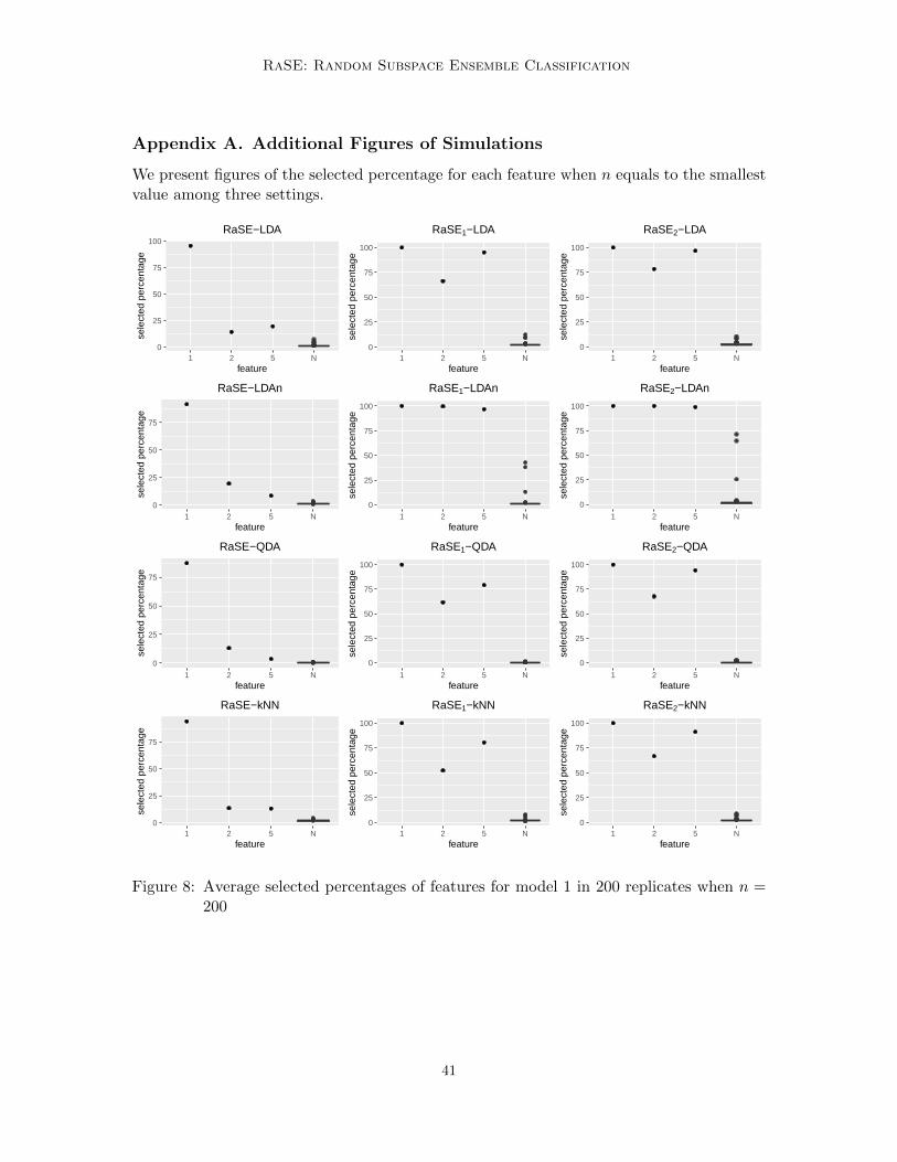
RaSE: Random Subspace Ensemble Classification
Appendix A. Additional Figures of Simulations
We present figures of the selected percentage for each feature when n equals to the smallestvalue among three settings.
0
25
50
75
100
1 2 5 Nfeature
sele
cted
per
cent
age
RaSE−LDA
0
25
50
75
100
1 2 5 Nfeature
sele
cted
per
cent
age
RaSE1−LDA
0
25
50
75
100
1 2 5 Nfeature
sele
cted
per
cent
age
RaSE2−LDA
0
25
50
75
1 2 5 Nfeature
sele
cted
per
cent
age
RaSE−LDAn
0
25
50
75
100
1 2 5 Nfeature
sele
cted
per
cent
age
RaSE1−LDAn
0
25
50
75
100
1 2 5 Nfeature
sele
cted
per
cent
age
RaSE2−LDAn
0
25
50
75
1 2 5 Nfeature
sele
cted
per
cent
age
RaSE−QDA
0
25
50
75
100
1 2 5 Nfeature
sele
cted
per
cent
age
RaSE1−QDA
0
25
50
75
100
1 2 5 Nfeature
sele
cted
per
cent
age
RaSE2−QDA
0
25
50
75
1 2 5 Nfeature
sele
cted
per
cent
age
RaSE−kNN
0
25
50
75
100
1 2 5 Nfeature
sele
cted
per
cent
age
RaSE1−kNN
0
25
50
75
100
1 2 5 Nfeature
sele
cted
per
cent
age
RaSE2−kNN
Figure 8: Average selected percentages of features for model 1 in 200 replicates when n =200
41

Tian and Feng
0
10
20
30
Nfeature
sele
cted
per
cent
age
RaSE−LDA
0
20
40
60
Nfeature
sele
cted
per
cent
age
RaSE1−LDA
0
20
40
60
Nfeature
sele
cted
per
cent
age
RaSE2−LDA
0
10
20
Nfeature
sele
cted
per
cent
age
RaSE−LDAn
0
25
50
75
100
Nfeature
sele
cted
per
cent
age
RaSE1−LDAn
0
25
50
75
100
Nfeature
sele
cted
per
cent
age
RaSE2−LDAn
0
5
10
15
20
25
Nfeature
sele
cted
per
cent
age
RaSE−QDA
0
10
20
30
40
Nfeature
sele
cted
per
cent
age
RaSE1−QDA
0
10
20
30
40
Nfeature
sele
cted
per
cent
age
RaSE2−QDA
0
10
20
30
Nfeature
sele
cted
per
cent
age
RaSE−kNN
0
20
40
60
Nfeature
sele
cted
per
cent
age
RaSE1−kNN
0
20
40
60
Nfeature
sele
cted
per
cent
age
RaSE2−kNN
Figure 9: Average selected percentages of features for model 1’ in 200 replicates when n =200
42
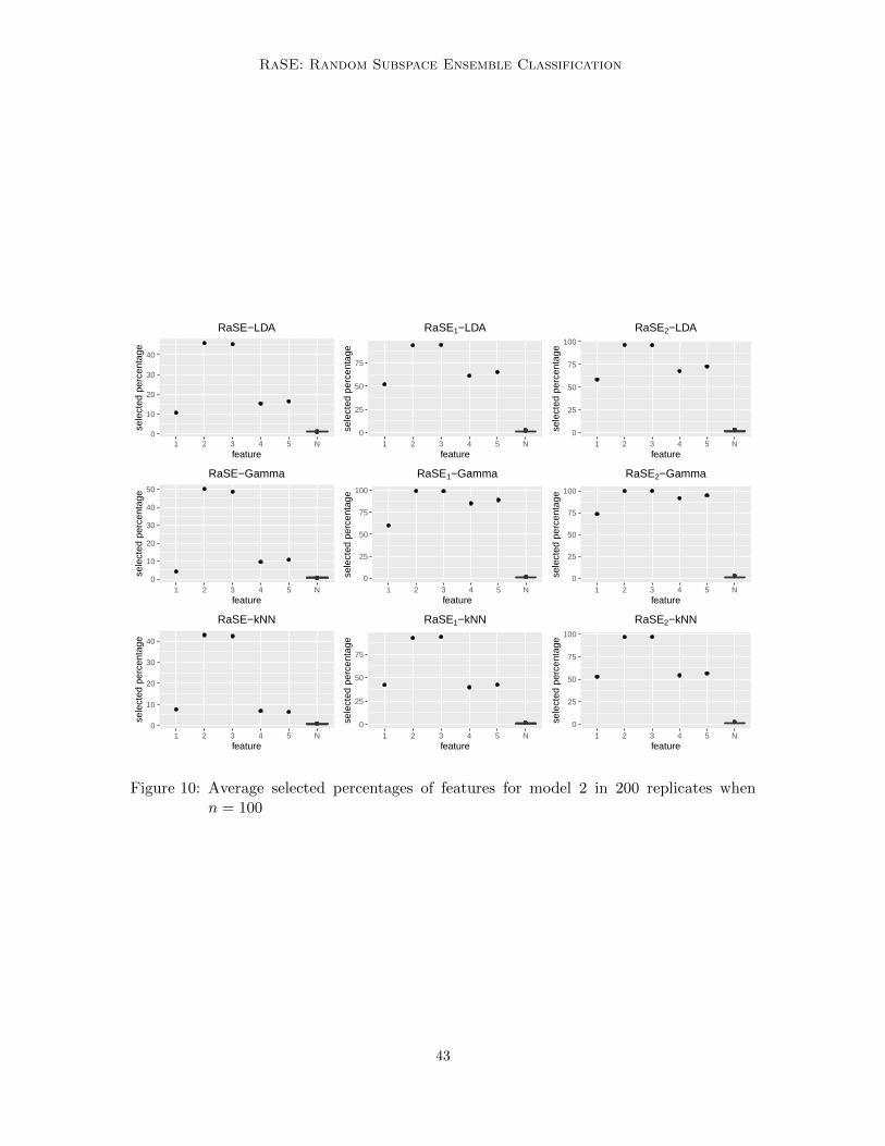
RaSE: Random Subspace Ensemble Classification
0
10
20
30
40
1 2 3 4 5 Nfeature
sele
cted
per
cent
age
RaSE−LDA
0
25
50
75
1 2 3 4 5 Nfeature
sele
cted
per
cent
age
RaSE1−LDA
0
25
50
75
100
1 2 3 4 5 Nfeature
sele
cted
per
cent
age
RaSE2−LDA
0
10
20
30
40
50
1 2 3 4 5 Nfeature
sele
cted
per
cent
age
RaSE−Gamma
0
25
50
75
100
1 2 3 4 5 Nfeature
sele
cted
per
cent
age
RaSE1−Gamma
0
25
50
75
100
1 2 3 4 5 Nfeature
sele
cted
per
cent
age
RaSE2−Gamma
0
10
20
30
40
1 2 3 4 5 Nfeature
sele
cted
per
cent
age
RaSE−kNN
0
25
50
75
1 2 3 4 5 Nfeature
sele
cted
per
cent
age
RaSE1−kNN
0
25
50
75
100
1 2 3 4 5 Nfeature
sele
cted
per
cent
age
RaSE2−kNN
Figure 10: Average selected percentages of features for model 2 in 200 replicates whenn = 100
43
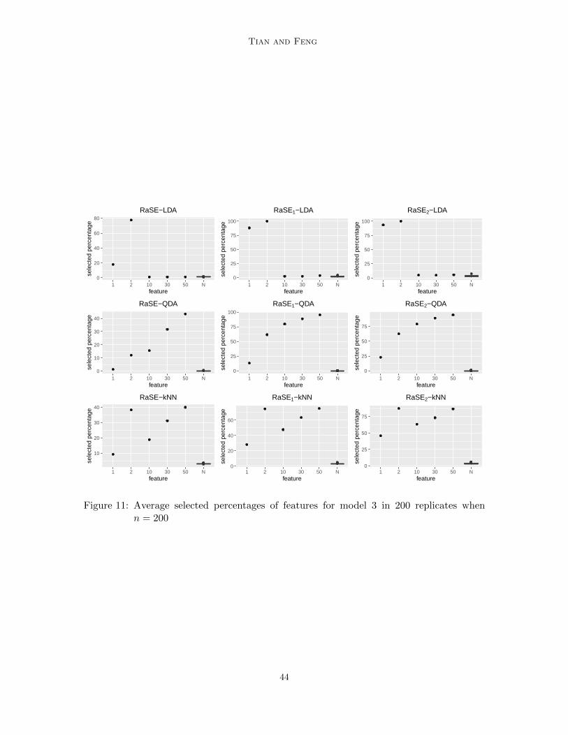
Tian and Feng
0
20
40
60
80
1 2 10 30 50 Nfeature
sele
cted
per
cent
age
RaSE−LDA
0
25
50
75
100
1 2 10 30 50 Nfeature
sele
cted
per
cent
age
RaSE1−LDA
0
25
50
75
100
1 2 10 30 50 Nfeature
sele
cted
per
cent
age
RaSE2−LDA
0
10
20
30
40
1 2 10 30 50 Nfeature
sele
cted
per
cent
age
RaSE−QDA
0
25
50
75
100
1 2 10 30 50 Nfeature
sele
cted
per
cent
age
RaSE1−QDA
0
25
50
75
1 2 10 30 50 Nfeature
sele
cted
per
cent
age
RaSE2−QDA
10
20
30
40
1 2 10 30 50 Nfeature
sele
cted
per
cent
age
RaSE−kNN
0
20
40
60
1 2 10 30 50 Nfeature
sele
cted
per
cent
age
RaSE1−kNN
0
25
50
75
1 2 10 30 50 Nfeature
sele
cted
per
cent
age
RaSE2−kNN
Figure 11: Average selected percentages of features for model 3 in 200 replicates whenn = 200
44

RaSE: Random Subspace Ensemble Classification
10
20
30
1 2 3 4 5 Nfeature
sele
cted
per
cent
age
RaSE−LDA
0
20
40
1 2 3 4 5 Nfeature
sele
cted
per
cent
age
RaSE1−LDA
0
20
40
60
1 2 3 4 5 Nfeature
sele
cted
per
cent
age
RaSE2−LDA
0
10
20
1 2 3 4 5 Nfeature
sele
cted
per
cent
age
RaSE−QDA
0
20
40
60
80
1 2 3 4 5 Nfeature
sele
cted
per
cent
age
RaSE1−QDA
0
25
50
75
100
1 2 3 4 5 Nfeature
sele
cted
per
cent
age
RaSE2−QDA
10
20
30
40
1 2 3 4 5 Nfeature
sele
cted
per
cent
age
RaSE−kNN
0
20
40
60
80
1 2 3 4 5 Nfeature
sele
cted
per
cent
age
RaSE1−kNN
0
25
50
75
1 2 3 4 5 Nfeature
sele
cted
per
cent
age
RaSE2−kNN
Figure 12: Average selected percentages of features for model 4 in 200 replicates whenn = 200
45

Tian and Feng
2
4
6
8
10
Nfeature
sele
cted
per
cent
age
RaSE−LDA
10
20
Nfeature
sele
cted
per
cent
age
RaSE1−LDA
0
10
20
30
Nfeature
sele
cted
per
cent
age
RaSE2−LDA
0
1
2
3
4
5
Nfeature
sele
cted
per
cent
age
RaSE−QDA
0
5
10
15
20
Nfeature
sele
cted
per
cent
age
RaSE1−QDA
0
5
10
15
20
25
Nfeature
sele
cted
per
cent
age
RaSE2−QDA
5.0
7.5
10.0
12.5
Nfeature
sele
cted
per
cent
age
RaSE−kNN
5
10
15
20
25
Nfeature
sele
cted
per
cent
age
RaSE1−kNN
0
10
20
30
Nfeature
sele
cted
per
cent
age
RaSE2−kNN
Figure 13: Average selected percentages of features for model 4’ in 200 replicates whenn = 200
46

RaSE: Random Subspace Ensemble Classification
Appendix B. Main Proofs
In the following proofs, for convenience, we use C to represent a positive constant, whichcould be different at different occurences.
B.1 Proof of Proposition 3
(i) The conditional probability is
P(y = 1|x) =π1f
(1)(x)
π1f (1)(x) + π0f (0)(x).
The definition of discriminative set is equivalent to
P(y = 1|x) = P(y = 1|xS), (14)
orP(y = 0|x) = P(y = 0|xS)
almost surely, which is also equivalent to
f (1)(x)
f (0)(x)=f
(1)S (xS)
f(0)S (xS)
. (15)
(ii) First, we observe the condition is equivalent to f (1)(x) = h(xS)f (0)(x). Taking
integration on both sides with respect to xSc , we get f(1)S (xS) = h(xS)f
(0)S (xS). Due to the
equivalence of (14) and (15), S is a discriminative set.
B.2 Proof of Proposition 5
To facilitate our analysis, we first state the following lemma.
Lemma 26 A discriminative set S is unique, if it will not be a discriminative set anymoreafter removing any features from it.
Proof [Proof of Lemma 26] Suppose the conclusion is not correct, then there exist twodifferent discriminative sets S1 and S2 satisfying such a property, that is, deleting anyfeatures from them leads to non-discriminative sets. Then according to Proposition 3 (i),we have
f(1)S1
(xS1)
f(0)S1
(xS1)=f
(1)S2
(xS2)
f(0)S2
(xS2), (16)
almost surely w.r.t Px, where Px = π0P(0) + π1P(1). Since f (0), f (1) are supported on thewhole Rp, Px dominates the Lebesgue measure. Combined with the explicit form of density
functions of Gaussian distribution and denoting ΩS1,S1 = (Σ(1)S1,S1
)−1 − (Σ(0)S1,S1
)−1,ΩS2,S2 =
(Σ(1)S2,S2
)−1 − (Σ(0)S2,S2
)−1, δS1 = (Σ(0)S1,S1
)−1µ(0)S1− (Σ
(1)S1,S1
)−1µ(1)S1, δS2 = (Σ
(0)S2,S2
)−1µ(0)S2−
(Σ(1)S2,S2
)−1µ(1)S2
, it can be obtained from (4) and (16) that
c+1
2xTS1
ΩS1,S1xS1 + δTS1xS1 = c′ +
1
2xTS2
ΩS2,S2xS2 + δTS2xS2 ,
47

Tian and Feng
where c, c′ are constants irrelative to S1, S2. Considering the combined vector xS1∪S2 , thereexists some matrix Ω and vector δ such that the equation above can be simplified as
xTS1∪S2ΩxS1∪S2 + δTxS1∪S2 + c− c′ = 0, (17)
for almost every xS1∪S2 in the Euclidean space. Since S1 is a discriminative set, by Exam-ple 2, for every feature j ∈ S1, the corresponding row of ΩS1,S1 is not zero vector or thecorresponding component of δS1 is not zero. The same argument holds for S2 as well. SinceS1\S2 and S2\S1 are not empty, at least one of Ω and δ contain non-zero components.However, it’s obvious that (17) cannot hold for almost every xS1∪S2 in Euclidean space,which leads to contradiction. Thus S∗ is unique.
Now let’s proceed on the proof of Proposition 5.By Definition 1, the minimal discriminative set S∗ satisfies the property described in
Lemma 26, therefore by this lemma S∗ is obviously unique, which implies (i).For (ii), if there exists a discriminative set S 6⊇ S∗, we can remove elements from S until
we arrive at a discriminative set S′ that satisfies the property stated in Lemma 26. It’sapparent S′ 6= S∗, which contradicts with Lemma 26.
(iii) is trivial from Definition 1.
B.3 Proof of Proposition 8
By Definition 6 and the fact that deg(S) = |S|+ 1, it’s easy to obtain that
RICn(S) =2
n
n∑i=1
1(yi = 0)
[((µ
(1)S )T Σ−1
S,S − (µ(0)S )T Σ−1
S,S)xi,S +1
2(µ
(0)S )T Σ−1
S,Sµ(0)S
−1
2(µ
(1)S )T Σ−1
S,Sµ(1)S
]+
2
n
n∑i=1
1(yi = 1)
[((µ
(0)S )T Σ−1
S,S − (µ(1)S )T Σ−1
S,S)xi,S
+1
2(µ
(1)S )T Σ−1
S,Sµ(1)S −
1
2(µ
(0)S )T Σ−1
S,Sµ(0)S
]+ cn · (|S|+ 1)
= 2π0
[((µ
(1)S )T Σ−1
S,S − (µ(0)S )T Σ−1
S,S)µ(0)S +
1
2(µ
(0)S )T Σ−1
S,Sµ(0)S −
1
2(µ
(1)S )T Σ−1
S,Sµ(1)S
]+ 2π1
[((µ
(0)S )T Σ−1
S,S − (µ(1)S )T Σ−1
S,S)µ(1)S +
1
2(µ
(1)S )T Σ−1
S,Sµ(1)S −
1
2(µ
(0)S )T Σ−1
S,Sµ(0)S
]+ cn · (|S|+ 1)
= −(µ(1)S − µ
(0)S )T Σ−1
S,S(µ(1)S − µ
(0)S ) + cn · (|S|+ 1),
which completes the proof.
B.4 Proof of Proposition 9
By Definition 6 and the fact deg(S) = |S|(|S|+ 3)/2 + 1, it’s easy to obtain that
RICn(S) =2
n
n∑i=1
1(yi = 0)
[1
2xTi,S((Σ
(0)S,S)−1 − (Σ
(1)S,S)−1)xi,S + ((µ
(1)S )T (Σ
(1)S,S)−1
48

RaSE: Random Subspace Ensemble Classification
− (µ(0)S )T (Σ
(0)S,S)−1)xi,S +
1
2(µ
(0)S )T (Σ
(0)S,S)−1µ
(0)S −
1
2(µ
(1)S )T (Σ
(1)S,S)−1µ
(1)S
+ log(|Σ(0)S,S |)− log(|Σ(1)
S,S |)]
+2
n
n∑i=1
1(yi = 1)
[1
2xTi,S((Σ
(1)S,S)−1 − (Σ
(0)S,S)−1)xi,S
+ ((µ(0)S )T (Σ
(0)S,S)−1 − (µ
(1)S )T (Σ
(1)S,S)−1)xi,S +
1
2(µ
(1)S )T (Σ
(1)S,S)−1µ
(1)S
− 1
2(µ
(0)S )T (Σ
(0)S,S)−1µ
(0)S + log(|Σ(1)
S,S |)− log(|Σ(0)S,S |)
]+ cn · (|S|(|S|+ 3)/2 + 1).
Denote the observations with class r as x(r)i
nri=1, r = 0, 1. And it holds that
1
n
n∑i=1
1(yi = 0)[xTi,S((Σ
(0)S,S)−1 − (Σ
(1)S,S)−1)xi,S
]=n0
n· 1
n0
n0∑i=1
[(x
(0)i,S)T ((Σ
(0)S,S)−1 − (Σ
(1)S,S)−1)x
(0)i,S
]= π0 ·
1
n0
n0∑i=1
Tr[((Σ
(0)S,S)−1 − (Σ
(1)S,S)−1)x
(0)i,S(x
(0)i,S)T
]= π0Tr
[((Σ
(0)S,S)−1 − (Σ
(1)S,S)−1)
1
n0
n0∑i=1
x(0)i,S(x
(0)i,S)T
]= π0Tr
[((Σ
(0)S,S)−1 − (Σ
(1)S,S)−1)(µ
(0)S (µ
(0)S )T + Σ
(0)S,S)
]= π0(µ
(0)S )T ((Σ
(0)S,S)−1 − (Σ
(1)S,S)−1)µ
(0)S + π0Tr
[((Σ
(0)S,S)−1 − (Σ
(1)S,S)−1)Σ
(0)S,S
].
Similarly we have
1
n
n∑i=1
1(yi = 1)[xTi,S((Σ
(1)S,S)−1 − (Σ
(0)S,S)−1)xi,S
]= π1(µ
(1)S )T ((Σ
(1)S,S)−1 − (Σ
(0)S,S)−1)µ
(1)S + π1Tr
[((Σ
(1)S,S)−1 − (Σ
(0)S,S)−1)Σ
(1)S,S
].
Combining with the fact
1
n
n∑i=1
1(yi = r)xi,S = πrµ(r)S , r = 0, 1,
we obtain that
RICn(S) = −(µ(1)S − µ
(0)S )T [π1(Σ
(0)S,S)−1 + π0(Σ
(1)S,S)−1](µ
(1)S − µ
(0)S )
+ Tr[((Σ(1)S,S)−1 − (Σ
(0)S,S)−1)(π1Σ
(1)S,S − π0Σ
(0)S,S)] + (π1 − π0)(log |Σ(1)
S,S | − log |Σ(0)S,S |)
+ cn · (|S|(|S|+ 3)/2 + 1),
which completes the proof.
49

Tian and Feng
B.5 Proof of Theorem 10
Denote gn(α′) = π1g(1)n (α′)− π0g
(0)n (α′). By the definition of αiNi=1, it holds that
gn(α) = 0,when α /∈ αiNi=1.
Recall that x|y = 0 ∼ P(0),x|y = 1 ∼ P(1), where P(0),P(1) are the corresponding cumula-tive distribution functions. We have
E[R(CRaSEn )] = π0
∫X
P(νn(x) > α)dP(0) + π1
∫X
P(νn(x) ≤ α)dP(1).
For given x and the corresponding α′ = µn(x), we can construct a random variable T =∑B1j=1 1
CSj∗n (x) = 1
∼ Bin(B1, α
′). Then∫X
P(νn(x) ≤ α)dP(1) =
∫[0,1]
P(T ≤ B1α)dG(1)n (α′).
Similarly, ∫X
P(νn(x) > α)dP(0) = 1−∫
[0,1]P(T ≤ B1α)dG(0)
n (α′).
This leads to
E[R(CRaSEn )] = π0 +
∫[0,1]
P(T ≤ B1α)dGn(α′),
where Gn(α′) = π1G(1)n (α′)− π0G
(0)n (α′). And there also holds that
R(CRaSE∗n ) = π0P(0)(µn(x) > α) + π1P(1)(µn(x) < α)
+1
2[π0P(0)(µn(x) = α)) + π1P(1)(µn(x) = α)]
= π0(1−G(0)n (α)) + π1G
(1)n (α) +
1
2[π0g
(0)n (α)− π1g
(1)n (α)]
= π0 +Gn(α)− 1
2gn(α),
where gn(α′) = π1g(1)n (α′)− π0g
(0)n (α′). This implies
E[R(CRaSEn )]−R(CRaSE∗n ) =
∫[0,1]
[P(T ≤ B1α)− 1α′≤α]dGn(α′) +1
2gn(α). (18)
(i) When α /∈ αiNi=1, gn(α) = 0 holds. For α′ ∈ αiNi=1, by Hoeffding’s inequality(Petrov, 2012), we obtain that
|P(T ≤ B1α)− 1α′≤α|≤ P(T −B1α
′ > B1(α− α′))1α′≤α + P(B1α′ − T ≥ B1(α′ − α))1α′>α
≤ exp−2B1(α′ − α)2≤ exp −CαB1 ,
where Cα = min1≤i≤N
|α−αi|2. This leads to the final bound |E[R(CRaSEn )]−R(CRaSE∗n )| ≤
exp −CαB1.
50

RaSE: Random Subspace Ensemble Classification
(ii) When α = αi0 , i0 ∈ 1, 2, . . . , N, for α′ 6= αi0 , we have
|P(T ≤ B1α)− 1α′≤α| ≤ exp−2B1(α′ − α)2,
leading to∑i 6=i0
|P(T ≤ B1α)− 1α′≤α|gn(αi) = exp −CαB1∑i 6=i0
gn(αi) ≤ exp −CαB1 ,
where Cα = 2 min1≤i≤N
|α− αi|2 = 2 mini 6=i0|αi0 − αi|2. Therefore, again by (18), we have
|E[R(CRaSE)]−R(CRaSE∗n )| ≤∣∣∣∣[P(T ≤ B1αi0)− 1] · gn(αi0) +
1
2gn(αi0)
∣∣∣∣+exp −CαB1 .
By Berry-Esseen theorem (Esseen, 1956),
P(T ≤ B1αi0) = P
(T −B1αi0√
B1(αi0(1− αi0))≤ 0
)=
1
2+O
(1√B1
), (19)
as B1 →∞. Eventually there holds that
|E[R(CRaSE)]−R(CRaSE∗n )| ≤ O(
1√B1
).
This completes the proof.
B.6 Proof of Theorem 11
Referring to the proof of the bound on MC-variance in Cannings and Samworth (2017), itcan be obtained that
Var
(∫Rp1νn(x)>αdP(0)
)≤ 2
∫[0,1]
∫[0,α′′]
P(T ′ ≤ B1α)P(T ′′ > B1α)dG(0)n (α′)dG(0)
n (α′′),
where given x, T ′ ∼ Bin(B1, α′), T ′′ ∼ Bin(B1, α
′′) and T ′, T ′′ are independent.
(i) For α /∈ α(0)i
N0i=1 ∪ α
(1)i
N1i=1: constant C
(0)α = 2 min
1≤i≤N0
(|α − α(0)i |2) > 0, C
(1)α =
2 min1≤i≤N1
(|α− α(1)i |2) > 0. If α ≤ α′ ≤ α′′: Then by Hoeffding’s inequality, we have
P(T ′ ≤ B1α) = P(T ′ −B1α′ ≤ B1(α− α′)) ≤ exp−B1C
(0)α . (20)
If α′ ≤ α′′ ≤ α: Similarly we have
P(T ′′ > B1α) ≤ exp−B1C(0)α . (21)
If α′ ≤ α ≤ α′′: We have both (20) and (21).
Thus we always have
P(T ′ ≤ B1α)P(T ′′ > B1α) ≤ exp−B1C(0)α .
51

Tian and Feng
Since here the integration actually is the finite summation, it implies that
Var
(∫X1νn(x)>αdP(0)
)≤ exp−B1C
(0)α .
Since α /∈ α(1)i
N1i=1: We can obtain the similar conclusion that
Var
(∫X1νn(x)≤αdP(1)
)≤ exp−B1C
(1)α .
Thus for any α /∈ α(0)i
N0i=1∪α
(1)i
N1i=1, setting Cα = 2 min
1≤i≤N01≤j≤N1
(|α−α(0)i |2, |α−α
(1)j |2) =
min(C(0)α , C
(1)α ) > 0, then by the convexity, we have
Var(R(CRaSEn )
)= Var
(π0
∫X1νn(x)>αdP(0) + π1
∫X1νn(x)≤αdP(1)
)≤ π0Var
(∫X1νn(x)>αdP(0)
)+ π1Var
(∫X1νn(x)≤αdP(1)
)≤ exp−B1Cα.
(ii) For α = α(0)i0
or α(1)i1
: Without loss of generality, suppose α = α(0)i0
. When α′ < α′′,similar to (i), there exists positive number C ′α such that
P(T ′ ≤ B1α)P(T ′′ > B1α) ≤ exp−B1C′α.
When α′ = α′′ = α(0)i0
, similar to (19), there holds
P(T ′ ≤ B1α)P(T ′′ > B1α) =1
4+O
(1√B1
).
Thus it holds
Var
(∫X1νn(x)>αdP
(0)
)≤ 1
2(g(0)n (α
(0)i0
))2 +O
(1√B1
).
And similar results hold for Var(∫X 1νn(x)≤αdP
(1)). Eventually we would have
Var(R(CRaSEn )
)≤ π0Var
(∫X1νn(x)>αdP(0)
)+ π1Var
(∫X1νn(x)≤αdP(1)
)≤ 1
2
[π0(g(0)
n (α))2 + π1(g(1)n (α))2
]+O
(1√B1
),
which completes the proof.
52

RaSE: Random Subspace Ensemble Classification
B.7 Proof of Proposition 12
(i) Due to Proposition 3, this is trivial to be seen to hold here.
(ii) First let’s consider subspace S = S′ ∪ j, where |S′| ≥ 1, j /∈ S′. The conditional
densities of j|S′ are denoted as f(0)j|S′ , f
(1)j|S′ and the components of xS corresponding
to S′ and j are xS′ ,xj , respectively. The definition of KL divergence and Fubinitheorem incur
KL(f(0)S ||f
(1)S ) = E
xS∼f(0)S
log
(f
(0)S′ (xS′)
f(1)S′ (xS′)
)+ log
f (0)j|S′(xj)
f(1)j|S′(xj)
= E
xS′∼f(0)
S′
[log
(f
(0)S′ (xS′)
f(1)S′ (xS′)
)]+ E
xS′∼f(0)
S′
Exj∼f
(0)
j|S′log
f (0)j|S′(xj)
f(1)j|S′(xj)
= KL(f
(0)S′ ||f
(1)S′ ) + E
xS′∼f(0)
S′
[KL(f
(0)j|S′ ||f
(1)j|S′)
]≥ KL(f
(0)S′ ||f
(1)S′ ).
Here “=” holds if and only if f(0)j|S′(xj |xS′) = f
(1)j|S′(xj |xS′) a.s. with respect to P(0).
By induction, this indicates that for any S ⊇ S′ and S′ 6= ∅, there holds
KL(f(0)S ||f
(1)S ) ≥ KL(f
(0)S′ ||f
(1)S′ ). (22)
Note that in (22), by Proposition 3, if f(0)j|S′(xj |xS′) = f
(1)j|S′(xj |xS′) a.s. with respect
to P(0), we have
f(0)S (xS)
f(1)S (xS)
=f
(0)S′ (xS′)
f(1)S′ (xS′)
, a.s. , w.r.t. P(0). (23)
Similarly, we have
KL(f(1)S ||f
(0)S ) ≥ KL(f
(1)S′ ||f
(0)S′ ), (24)
where the “ = ” holds if and only if
f(1)S (xS)
f(0)S (xS)
=f
(1)S′ (xS′)
f(0)S′ (xS′)
, a.s. , w.r.t. P(1). (25)
If S 6⊇ S∗, consider S = S ∪ (S∗\S) ⊇ S∗, then by (i) and (22), there holds
π0KL(f(0)S ||f
(1)S ) + π1KL(f
(1)S ||f
(0)S ) ≤ π0KL(f
(0)
S||f (1)
S) + π1KL(f
(1)
S||f (0)
S) (26)
= π0KL(f(0)S∗ ||f
(1)S∗ ) + π1KL(f
(1)S∗ ||f
(0)S∗ ).
Then by Proposition 3, if the “=” holds in (26), due to (23) and (25), we have
f(0)S (xS)
f(1)S (xS)
=f
(0)
S(xS)
f(1)
S(xS)
=f
(0)S∗ (xS∗)
f(1)S∗ (xS∗)
, a.s. , w.r.t. Px = π0P(0) + π1P(1),
implying that S is a discriminative set but S 6⊇ S∗, which yields a contradiction.Therefore (ii) holds here.
53

Tian and Feng
(iii) holds since the full model SFull ⊇ S∗ and the KL divergence is monotone in the senseof (22) and (24).
B.8 Proof of Proposition 14
DenoteR0|1S (µ
(0)S ,µ
(1)S ,ΣS,S ,xS) = log
(f
(0)S (xS)
f(1)S (xS)
)=(µ
(0)S − µ
(1)S
)TΣ−1S,S
[xS − 1
2(µ(0)S + µ
(1)S )].
To eliminate any confusion and better illustrate the meaning of the gradient and second-
order derivative matrix, we will use∂R
0|1S
∂µ(0)S
,∂R
0|1S
∂µ(1)S
,∂R
0|1S
∂ΣS,Sto represent the gradient and use
∂2R0|1S
∂µ(0)S ∂ΣS,S
,∂2R
0|1S
∂µ(1)S ∂ΣS,S
,∂2R
0|1S
∂ΣS,S∂ΣS,Sto represent the second-order derivative matrix.
According to Brookes (2005) and Petersen and Pedersen (2012), with some calculationwe can obtain that
∂R0|1S
∂µ(0)S
= Σ−1S,S
(xS − µ(0)
S
),
∂R0|1S
∂µ(1)S
= Σ−1S,S
(xS − µ(1)
S
),
∂R0|1S
∂ΣS,S= Σ−1
S,S
(µ
(0)S − µ
(1)S
)(xS −
1
2(µ
(0)S + µ
(1)S )
)TΣ−1S,S ,
∂2R0|1S
∂µ(0)S ∂µ
(0)S
=∂2R
0|1S
∂µ(1)S ∂µ
(1)S
= −Σ−1S,S ,
∂2R0|1S
∂ΣS,S∂µ(0)S
= −(
Σ−1S,S ⊗ Σ−1
S,S
)(I|S| ⊗
(xS − µ(0)
S
)),
∂2R0|1S
∂ΣS,S∂µ(1)S
= −(
Σ−1S,S ⊗ Σ−1
S,S
)(I|S| ⊗
(xS − µ(1)
S
)),
∂2R0|1S
∂ΣS,S∂ΣS,S= −
[I|S| ⊗ Σ−1
S,S
(µ
(0)S − µ
(1)S
)(xS −
1
2(µ
(0)S + µ
(1)S )
)T+
(xS −
1
2(µ
(0)S + µ
(1)S )
)(µ
(0)S − µ
(1)S
)TΣ−1S,S ⊗ I|S|
](Σ−1S,S ⊗ Σ−1
S,S
),
where ⊗ is the Kronecker product.Then let’s check conditions in Assumption 3 one by one. Without loss of generality, for
(iii), we only check the case that xi,Si.i.d.∼ f
(0)S . And for (iv), (v), we only check the case
that xS ∼ f (0)S .
(i) It’s easy to see that the number of parameters in LDA model in p-dimensional space
is 2 + 2p+ p(p+1)2 , therefore κ1 = 2.
(ii) According to Assumption 4, we have
KL(f (0)||f (1)) =(µ(1) − µ(0)
)TΣ−1
(µ(1) − µ(0)
)54

RaSE: Random Subspace Ensemble Classification
≤ ‖µ(1)S∗ − µ
(0)S∗ ‖
22 · ‖Σ−1
S∗,S∗‖2≤ p∗(M ′)2m−1
≤ D(M ′)2m−1.
The similar conclusion holds for KL(f (1)||f (0)) as well.
(iii) For any (µ(0)S , µ
(1)S , ΣS,S):∥∥∥∥∥ 1
n
n∑i=1
∂2R0|1S
∂ΣS,S∂ΣS,S(µ
(0)S , µ
(1)S , ΣS,S ,xi)
∥∥∥∥∥max
≤
∥∥∥∥∥ 1
n
n∑i=1
∂2R0|1S
∂ΣS,S∂ΣS,S(µ
(0)S , µ
(1)S , ΣS,S ,xi)
∥∥∥∥∥2
≤ 2∥∥∥Σ−1
S,S(µ(0)S − µ
(1)S )∥∥∥
2·
∥∥∥∥∥ 1
n
n∑i=1
[xi,S −
1
2(µ
(0)S + µ
(1)S )
]∥∥∥∥∥2
·∥∥∥Σ−1
S,S
∥∥∥2
2
≤ 2∥∥∥Σ−1
S,S
∥∥∥3
2·∥∥∥µ(0)
S − µ(1)S
∥∥∥2·
∥∥∥∥∥ 1
n
n∑i=1
[xi,S −
1
2(µ
(0)S + µ
(1)S )
]∥∥∥∥∥2
.
When ‖µ(0)S − µ
(0)S ‖2, ‖µ
(1)S − µ
(1)S ‖2, ‖ΣS,S − ΣS,S‖F ≤ ζ < m, due to (28), it follows
that
‖Σ−1S,S − Σ−1
S,S‖2 ≤1m2 ‖ΣS,S − ΣS,S‖2
1− 1m‖ΣS,S − ΣS,S‖2
≤1m2 ‖ΣS,S − ΣS,S‖F
1− 1m‖ΣS,S − ΣS,S‖F
≤ ζ
m2 −mζ,
which leads to
‖Σ−1S,S‖2 ≤ ‖Σ
−1S,S‖2 + ‖Σ−1
S,S − Σ−1S,S‖2 ≤
1
m− ζ.
In addition, we have
‖µ(0)S − µ
(1)S ‖2 ≤ ‖µ
(0)S − µ
(0)S ‖2 + ‖µ(1)
S − µ(1)S ‖2 + ‖µ(0)
S − µ(1)S ‖2 . D
12M ′.
Without loss of generality, consider xi,Si.i.d.∼ f
(0)S , it holds that∥∥∥∥∥ 1
n
n∑i=1
[xi,S −
1
2(µ
(0)S + µ
(1)S )
]∥∥∥∥∥2
≤
∥∥∥∥∥ 1
n
n∑i=1
(xi,S − µ(0)
S
)∥∥∥∥∥2
+1
2‖µ(0)
S − µ(0)S ‖2
+1
2‖µ(1)
S − µ(1)S ‖2 +
1
2‖µ(0)
S − µ(1)S ‖2
.
∥∥∥∥∥ 1
n
n∑i=1
(xi,S − µ(0)
S
)∥∥∥∥∥2
+D12M ′.
By Proposition 1 in Hsu et al. (2012), since 1n
∑ni=1(xi,S − µ(0)
S ) ∼ N(0, 1nΣS,S), it
follows that
P
∥∥∥∥∥ 1
n
n∑i=1
(xi,S − µ(0)
S
)∥∥∥∥∥2
>
√1
nTr(ΣS,S) + 2
√Tr(Σ2
S,S) · εn
+ 2‖ΣS,S‖2ε
≤ exp−nε.
55

Tian and Feng
And due to Assumption 4, we have
Tr(ΣS,S) ≤ D‖ΣS,S‖max ≤ DM,
Tr(Σ2S,S) = ‖ΣS,S‖2F ≤ D2‖ΣS,S‖2max ≤ D2M2,
‖ΣS,S‖2 ≤ D‖ΣS,S‖max ≤ DM,
yielding
P
∥∥∥∥∥ 1
n
n∑i=1
(xi,S − µ(0)
S
)∥∥∥∥∥2
>
√1
nDM + 2DM
√ε
n+ 2DMε
≤ exp−nε.
Therefore when ‖µ(0)S − µ
(0)S ‖2, ‖µ
(1)S − µ
(1)S ‖2, ‖ΣS,S − ΣS,S‖2 ≤ ζ, we have∥∥∥∥∥ 1
n
n∑i=1
∂2R0|1S
∂ΣS,S∂ΣS,S(µ
(0)S , µ
(1)S , ΣS,S ,xi)
∥∥∥∥∥max
. D12M
(∥∥∥∥∥ 1
n
n∑i=1
(xi,S − µ(0)
S
)∥∥∥∥∥2
+D12M
)
:= VS(xi,Sni=1),
andP (VS(xi,Sni=1) > CD) . exp−Cn.
Thus we can set κ2 = 1.
(iv) Σ−1S,S
(xS − µ(0)
S
)∼ N(0,Σ−1
S,S),Σ−1S,S
(xS − µ(1)
S
)∼ N(Σ−1
S,S(µ(0)S − µ
(1)S ),Σ−1
S,S) when
xS ∼ f (0)S . And also we have∥∥∥Σ−1
S,S
∥∥∥max≤∥∥∥Σ−1
S,S
∥∥∥2≤∥∥Σ−1
∥∥2≤ m−1.
Then each component of∂R
0|1S
∂µ(0)S
and∂R
0|1S
∂µ(1)S
is√m−1-subGaussian. On the other hand,
since Σ−1S,S
(xS − 1
2(µ(0)S + µ
(1)S ))∼ N
(12Σ−1
S,S(µ(0)S − µ
(1)S ),Σ−1
S,S
)and∥∥∥Σ−1
S,S(µ(0)S − µ
(1)S )∥∥∥∞≤ D
12
∥∥∥Σ−1S,S
∥∥∥2·∥∥∥µ(0)
S − µ(1)S
∥∥∥∞≤ m−1M ′D
12 , (27)
it follows that each component of∂R
0|1S
∂ΣS,Sis m−1
√M ′D-subGaussian. Therefore κ3 = 1
2 .
(v) Notice that because of (27), we have∥∥∥ExS∼f
(0)S
[Σ−1S,S(xS − µ(1)
S )]∥∥∥∞
=∥∥∥Σ−1
S,S(µ(0)S − µ
(1)S )∥∥∥∞≤ m−1M ′D
12 ,
∥∥∥∥∥ExS∼f (0)S
[Σ−1S,S
(µ
(0)S − µ
(1)S
)(xS −
1
2(µ
(0)S + µ
(1)S )
)TΣ−1S,S
]∥∥∥∥∥max
56

RaSE: Random Subspace Ensemble Classification
=1
2
∥∥∥∥Σ−1S,S
(µ
(0)S − µ
(1)S
)(µ
(0)S − µ
(1)S
)TΣ−1S,S
∥∥∥∥max
≤ 1
2
∥∥∥Σ−1S,S(µ
(0)S − µ
(1)S )∥∥∥2
∞
≤ 1
2(m−1M ′)2D.
Therefore κ4 = 1.
(vi) It’s easy to see that(µ
(1)S − µ
(0)S
)TΣ−1S,S
[xS − 1
2(µ(0)S + µ
(1)S )]∼ N((µ
(1)S −µ
(0)S )TΣ−1
S,S(µ(1)S −
µ(0)S ), (µ
(1)S − µ
(0)S )TΣ−1
S,S(µ(1)S − µ
(0)S )). And there holds
(µ(1)S − µ
(0)S )TΣ−1
S,S(µ(1)S − µ
(0)S ) ≤
∥∥∥µ(1)S − µ
(0)S
∥∥∥2
2·∥∥∥Σ−1
S,S
∥∥∥2≤ m−1(M ′)2D,
which yields that log
(f
(0)S (xS)
f(1)S (xS)
)is M ′
√m−1D-subGaussian. So κ5 = 1
2 .
(vii) This can be easily derived from Lemma 28 and its proof.
(viii) This is obvious because of Lemma 31.(iii) and Assumption 4.(iii).
B.9 Proof of Theorem 15
First suppose that we have n0 observations of class 0 x(0)i
n0i=1 and n1 observations of class
1 x(1)i
n1i=1, where n0 + n1 = n. Define
G(0)n0,S
(θ′S) =1
n0
n0∑i=1
log
f (0)S (x
(0)i,S |θ′S)
f(1)S (x
(0)i,S |θ′S)
, G(1)n1,S
(θ′S) =1
n1
n1∑i=1
log
f (1)S (x
(1)i,S |θ′S)
f(0)S (x
(1)i,S |θ′S)
,for any θ′S . Denote RIC(S) = −2[π0G
(0)n0,S
(θS) + π1G(1)n1,S
(θS)], then RICn(S) = RIC(S) +cn deg(S).
Lemma 27 If Assumptions 1-3 holds, then we have
P
(sup
S:|S|≤D|RIC(S)− RIC(S)| > ε
). pDDκ1 exp
−Cn
(ε
Dκ1(Dκ3 +Dκ4)
)2
+ pDDκ1 exp−Cn · ε
D2κ1+κ2
+ pD exp
−Cn
( ε
Dκ5
)2.
Proof [Proof of Lemma 27] By Taylor expansion and mean-value theorem, there existsλ ∈ (0, 1) and θS = λθS + (1− λ)θS satisfying that
G(0)n0,S
(θS) = G(0)n0,S
(θS) +∇G(0)n0,S
(θS)T (θS − θS) +1
2(θS − θS)T∇2G
(0)n0,S
(θ)(θS − θS).
57

Tian and Feng
Notice that ∥∥∥∇G(0)n0,S
(θS)T (θS − θS)∥∥∥
2≤ Dκ1
∥∥∥∇G(0)n0,S
(θS)∥∥∥∞‖θS − θS‖∞,
and when ‖θS − θS‖2 ≤ ζ, we also have∣∣∣(θS − θS)T∇2G(0)n0,S
(θ)(θS − θS)∣∣∣ . Dκ1‖θS − θS‖2∞‖∇2G
(0)n0,S
(θ)‖max
≤ D2κ1‖θS − θS‖2∞ ·∣∣∣VS(x(0)
i,Sn0i=1)
∣∣∣ .Since nr ∼ Bin(n, πr), r = 0, 1, by Hoeffding’s inequality, we have
P(|nr − nπr| > 0.5nπr) . exp−Cn, r = 0, 1.
Because of Assumption 3.(iv), given n0, each component of n0∇G(0)n0,S
(θS) is n0
√2C3D
κ3-subGaussian, then the tail bound in the below holds:
P
(∥∥∥∇G(0)n0,S
(θS)− ExS∼f
(0)S
∇θSLS(x;θ)∥∥∥∞> ε
∣∣∣∣∣n0
). Dκ1 exp
−Cn0
( ε
Dκ3
)2.
Then according to all conclusions above, we have
P(|G(0)n0,S
(θS)−KL(f(0)S ||f
(1)S )| > ε)
≤ En0 [P(|G(0)n0,S
(θS)−KL(f(0)S ||f
(1)S )| > ε||n0 − nπ0| ≤ 0.5nπ0)] + P(|n0 − nπ0| > 0.5nπ0)
≤ En0P(∣∣∣G(0)
n0,S(θS)−KL(f
(0)S ||f
(1)S )∣∣∣ > ε/3
∣∣∣|n0 − nπ0| ≤ 0.5nπ0
)+
+ En0P
(∥∥∥∇G(0)n0,S
(θS)− ExS∼f
(0)S
∇G(0)n0,S
(θS)∥∥∥∞> CDκ3
∣∣∣∣∣|n0 − nπ0| ≤ 0.5nπ0
)+ P
(CDκ1(Dκ3 +Dκ4)‖θS − θS‖∞ > ε/3
)+ P
(0.5CD2κ1+κ2‖θS − θS‖2∞ > ε/3
)+ En0P
(VS(x(0)
i,Sn0i=1) > CDκ2
∣∣∣∣∣|n0 − nπ0| ≤ 0.5nπ0
)+ P(|n0 − nπ0| > 0.5nπ0) + P(D
12κ1‖θS − θS‖∞ > ζ)
. Dκ1 exp
−Cn
(ε
Dκ1(Dκ3 +Dκ4)
)2
+Dκ1 exp−Cn · ε
D2κ1+κ2
+ exp
−Cn
( ε
Dκ5
)2,
which yields
P(|π0G(0)n0,S
(θS)− π0KL(f(0)S ||f
(1)S )| > ε) . Dκ1 exp
−Cn
(ε
Dκ1(Dκ3 +Dκ4)
)2
+Dκ1 exp−Cn · ε
D2κ1+κ2
+ exp
−Cn
( ε
Dκ5
)2.
58

RaSE: Random Subspace Ensemble Classification
Similarly, there holds
P(|π1G(1)n1,S
(θS)− π1KL(f(1)S ||f
(0)S )| > ε) . Dκ1 exp
−Cn
(ε
Dκ1(Dκ3 +Dκ4)
)2
+Dκ1 exp−Cn · ε
D2κ1+κ2
+ exp
−Cn
( ε
Dκ5
)2.
Since RIC(S) = −2[π0G(0)n0,S
(θS) + π1G(1)n1,S
(θS)], we obtain that
P(|RIC(S)− RIC(S)| > ε
). Dκ1 exp
−Cn
(ε
Dκ1(Dκ3 +Dκ4)
)2
+Dκ1 exp−Cn · ε
D2κ1+κ2
+ exp
−Cn
( ε
Dκ5
)2.
Due to the union bound over all(pD
)= O(pD) possible subsets, we obtain the conclusion.
Let’s now prove Theorem 15.
(i) It’s easy to see that
P
supS:S⊇S∗|S|≤D
RICn(S) ≥ infS:S 6⊇S∗|S|≤D
RICn(S)
≤ P
RIC(S∗) + cn supS:|S|≤D
deg(S) + ∆/3 ≥ infS:S 6⊇S∗|S|≤D
RIC(S)−∆/3
+ P
(sup
S:|S|≤D|RIC(S)− RIC(S)| > ∆/3
)
≤ P(cn supS:|S|≤D
deg(S) ≥ ∆/3) + P
(sup
S:|S|≤D|RIC(S)− RIC(S)| > ∆/3
)
. pDDκ1 exp
−Cn
(∆
Dκ1(Dκ3 +Dκ4)
)2
+ pDDκ1 exp
−Cn
(∆
D2κ1+κ2
)
+ pD exp
−Cn
(∆
Dκ5
)2
→ 0.
59

Tian and Feng
(ii) Similar to above, we have
P
RICn(S∗) ≥ infS:S 6⊇S∗|S|≤D
RICn(S)
≤ P
RIC(S∗) + cn deg(S∗) + ∆/3 ≥ infS:S 6⊇S∗|S|≤D
RIC(S)−∆/3
+ P
(sup
S:|S|≤D|RIC(S)− RIC(S)| > ∆/3
)
. pDDκ1 exp
−Cn
(∆
Dκ1(Dκ3 +Dκ4)
)2
+ pDDκ1 exp
−Cn
(∆
D2κ1+κ2
)
+ pD exp
−Cn
(∆
Dκ5
)2
→ 0.
Besides, it holds
P
RICn(S∗) ≥ infS:S⊇S∗|S|≤D
RICn(S)
≤ P (RIC(S∗) + cn deg(S∗) + cn/3 ≥ RIC(S∗) + cn(deg(S∗) + 1)− cn/3)
+ P
(sup
S:|S|≤D|RIC(S)− RIC(S)| > cn/3
)
. pDDκ1 exp
−Cn
(cn
Dκ1(Dκ3 +Dκ4)
)2
+ pDDκ1 exp−Cn
( cnD2κ1+κ2
)+ pD exp
−Cn
( cnDκ5
)2
→ 0.
Therefore we have
P(
RICn(S∗) 6= infS:|S|≤D
RICn(S)
)
≤ P
RICn(S∗) ≥ infS:S 6⊇S∗|S|≤D
RICn(S)
+ P
RICn(S∗) ≥ infS:S⊇S∗|S|≤D
RICn(S)
60

RaSE: Random Subspace Ensemble Classification
. pDDκ1 exp
−Cn
(cn
Dκ1(Dκ3 +Dκ4)
)2
+ pDDκ1 exp−Cn
( cnD2κ1+κ2
)+ pD exp
−Cn
( cnDκ5
)2
→ 0,
which is because cn ∆. This completes the proof.
B.10 Proof of Theorem 18
Lemma 28 For arbitrary ε ∈ (0,m−1), we have the following conclusions:
(i) P(‖(µ(1) − µ(0))− (µ(1) − µ(0))‖∞ > ε) . p exp−Cnε2, r = 0, 1;
(ii) P
supS1:|S1|≤DS2:|S2|≤D
‖ΣS1,S2 − ΣS1,S2‖∞ > ε
. p2 exp−Cn ·
(εD
)2+ p exp
−Cn · εD
;
(iii) P
(sup
S:|S|≤D‖ΣS,S − ΣS,S‖2 > ε
). p2 exp
−Cn ·
(εD
)2+ p exp
−Cn · εD
;
(iv) P
(sup
S:|S|≤D‖Σ−1
S,S − Σ−1S,S‖2 > ε
). p2 exp
−Cn ·
(εD
)2+ p exp
−Cn · εD
.
Proof [Proof of Lemma 28] For (i), because ‖Σ‖max ≤M , for any j = 1, . . . , p and r = 0, 1,
µ(r)j − µ
(r)j is a
√M -subGaussian variable. By the tail bound and union bound, we have
P(‖µ(r) − µ(r)‖∞ > ε) ≤p∑j=1
P(|µ(r)j − µ
(r)j | > ε) . p exp−Cnε2, r = 0, 1,
which leads to (i). Denote Σ = (σij)p×p, Σ = (σij)p×p. To show (ii), similar to Bickel et al.(2008), we have
P(
maxi,j|σij − σij | > ε
). p2 exp−Cnε2+ p exp−Cnε.
And it yields
P
supS1:|S1|≤DS2:|S2|≤D
‖ΣS1,S2 − ΣS1,S2‖∞ > ε
= P
supS1:|S1|≤DS2:|S2|≤D
supi∈S1
∑j∈S2
|σij − σij | > ε
≤ P
(D ·max
i,j|σij − σij | > ε
). p2 exp
−Cn ·
( εD
)2
+ p exp−Cn · ε
D
.
61

Tian and Feng
Since ΣS,S − ΣS,S is symmetric, we have ‖ΣS,S − ΣS,S‖2 ≤ ‖ΣS,S − ΣS,S‖∞ (Bickel et al.(2008)). For (iv), firstly because the operator norm is sub-multiplicative, we have
‖Σ−1S,S − Σ−1
S,S‖2 = ‖Σ−1S,S(ΣS,S − ΣS,S)Σ−1
S,S‖2≤ ‖Σ−1
S,S‖2 · ‖ΣS,S − ΣS,S‖2 · ‖Σ−1S,S‖2
≤ (‖Σ−1S,S − Σ−1
S,S‖2 + ‖Σ−1S,S‖2) · ‖ΣS,S − ΣS,S‖2 · ‖Σ−1
S,S‖2,
leading to
‖Σ−1S,S − Σ−1
S,S‖2 ≤‖Σ−1
S,S‖22 · ‖ΣS,S − ΣS,S‖21− ‖ΣS,S − ΣS,S‖2 · ‖Σ−1
S,S‖2≤
1m2 ‖ΣS,S − ΣS,S‖2
1− 1m‖ΣS,S − ΣS,S‖2
. (28)
Then we obtain that
P
(sup
S:|S|≤D‖Σ−1
S,S − Σ−1S,S‖2 > ε
)≤ P
(‖ΣS,S − ΣS,S‖2 >
1
2m
)+ P
(2
m2‖ΣS,S − ΣS,S‖2 > ε
)≤ 2P
(sup
S:|S|≤D‖ΣS,S − ΣS,S‖2 >
m2
2ε
).
Then by applying (iii), we get (iv) immediately.
Lemma 29 Define δS = Σ−1S,S(µ
(1)S − µ
(0)S ) for any subset S. For ∀S = S ∪ S∗, where
S ∩ S∗ = ∅, we have
δS = Σ−1S,S
(µ(1)
S− µ(0)
S) = Σ−1
S,S
(µ
(1)S − µ
(0)S
µ(1)S∗ − µ
(0)S∗
)=
(0δS∗
).
Proof [Proof of Lemma 29] First, when S = SFull, we know that
δS = Σ−1S,S
(µ(1)
S− µ(0)
S) = Σ−1
S,S
(µ
(1)S − µ
(0)S
µ(1)S∗ − µ
(0)S∗
)=
(0∗
).
Then combined with the matrix decomposition
Σ−1S,S
=
((ΣS,S − ΣS,S∗Σ
−1S∗,S∗ΣS∗,S)−1 −Σ−1
S,SΣS,S∗(ΣS∗,S∗ − ΣS∗,SΣ−1S,SΣS,S∗)
−1
−Σ−1S∗,S∗ΣS∗,S(ΣS,S − ΣS,S∗Σ
−1S∗,S∗ΣS∗,S)−1 (ΣS∗,S∗ − ΣS∗,SΣ−1
S,SΣS,S∗)−1
),
it can be noticed that
(ΣS,S−ΣS,S∗Σ−1S∗,S∗ΣS∗,S)−1(µ
(1)S −µ
(0)S ) = Σ−1
S,SΣS,S∗(ΣS∗,S∗−ΣS∗,SΣ−1S,SΣS,S∗)
−1(µ(1)S∗−µ
(0)S∗ ).
62

RaSE: Random Subspace Ensemble Classification
Also since there holds that
(ΣS∗,S∗−ΣS∗,SΣ−1S,SΣS,S∗)
−1 = Σ−1S∗,S∗−Σ−1
S∗,S∗ΣS∗,S(−ΣS,S+ΣS,S∗Σ−1S∗,S∗ΣS∗,S)−1ΣS,S∗Σ
−1S∗,S∗ ,
it can be easily verified that the “*” part is actually δS∗ . Therefore the conclusion holdswith S = SFull.
For general S ⊇ S∗, notice that SFull = (SFull\S) ∪ S, with the same procedure, we canobtain that
δSFull= Σ−1(µ(1) − µ(0)) =
(0δS
).
And since
δSFull=
(0δS∗
),
we reach the conclusion.
Lemma 30 For ∀S which satisfies S 6⊇ S∗, let S∗ = S∗\S, then∥∥∥ΣS∗,SΣ−1S,S
(µ
(1)S − µ
(0)S
)−(µ
(1)S∗ − µ
(0)S∗
)∥∥∥2≥ γm.
Proof [Proof of Lemma 30] Let S = S ∪ S∗, due to Lemma 29, it’s easy to see that thereholds
Σ−1S,S
(µ
(1)S − µ
(0)S
µ(1)
S∗− µ(0)
S∗
)=
(∗δ′S∗
), (29)
where
Σ−1S,S
=
((ΣS,S − ΣS,S∗Σ
−1S∗,S∗
ΣS∗,S)−1 −Σ−1S,SΣS,S∗(ΣS∗,S∗ − ΣS∗,SΣ−1
S,SΣS,S∗)−1
−Σ−1S∗,S∗
ΣS∗,S(ΣS,S − ΣS,S∗Σ−1S∗,S∗
ΣS∗,S)−1 (ΣS∗,S∗ − ΣS∗,SΣ−1S,SΣS,S∗)
−1
),
(30)
and δ′S∗
consists of several components of δS∗ . Denote c = ΣS∗,SΣ−1S,S
(µ
(1)S − µ
(0)S
)−(
µ(1)
S∗− µ(0)
S∗
). Since Σ−1
S,Sis symmetric, combining with (29) we have
(ΣS∗,S∗ − ΣS∗,SΣ−1S,SΣS,S∗)
−1c = −δ′S∗,
leading to‖(ΣS∗,S∗ − ΣS∗,SΣ−1
S,SΣS,S∗)−1c‖2 = ‖δ′
S∗‖2 ≥ γ,
by Assumption 4.(iii). For the left-hand side:
‖(ΣS∗,S∗ − ΣS∗,SΣ−1S,SΣS,S∗)
−1c‖2≤ ‖c‖2 · ‖(ΣS∗,S∗ − ΣS∗,SΣ−1
S,SΣS,S∗)−1‖2
≤ ‖c‖2 · ‖Σ−1S,S‖2
≤ ‖c‖2 · λ−1min(ΣS,S)
63

Tian and Feng
≤ m−1‖c‖2,
which leads to ‖c‖2 ≥ γm.
Lemma 31 For LDA, RIC(S) = −(µ
(1)S − µ
(0)S
)TΣ−1S,S
(µ
(1)S − µ
(0)S
). It satisfies the fol-
lowing conclusions:
(i) If S ⊇ S∗, then RIC(S) = RIC(S∗);
(ii) For S = S∗ ∪ S, we have
RIC(S) = RIC(S)−[ΣS∗,SΣ−1
S,S
(µ
(1)S − µ
(0)S
)−(µ
(1)
S∗− µ(0)
S∗
)]T(
ΣS∗,S∗ − ΣS∗,SΣ−1S,SΣS,S∗
) [ΣS∗,SΣ−1
S,S
(µ
(1)S − µ
(0)S
)−(µ
(1)
S∗− µ(0)
S∗
)](iii) It holds
infS:|S|≤DS 6⊇S∗
RIC(S)− RIC(S∗) ≥ m3γ2.
Proof [Proof of Lemma 31]
(i) First let’s suppose (ii) is correct. For S ⊇ S∗, consider SFull = S∗ ∪S and S∗ ∩S = ∅,then by sparsity condition, we have(
∗0
)= Σ−1(µ(1) − µ(0)) = Σ−1
(µ
(1)S − µ
(0)S
µ(1)
S∗− µ(0)
S∗
).
Also by basic algebra, there holds
(ΣS,S−ΣS,S∗Σ−1S∗,S∗
ΣS∗,S)−1 = Σ−1S,S−Σ−1
S,SΣS,S∗(−ΣS∗,S∗+ΣS∗,SΣ−1S,SΣS,S∗)
−1ΣS∗,SΣ−1S,S .
(31)Combined with (30) and (31), it can be obtained that
ΣS∗,SΣ−1S,S
(µ
(1)S − µ
(0)S
)−(µ
(1)
S∗− µ(0)
S∗
)= 0,
yielding that RIC(SFull) = RIC(S). Since the same procedure can be conducted forarbitrary S ⊇ S∗, we complete the proof.
(ii) This can be directly calculated and simplified by applying (30) and (31).
(iii) It’s easy to see that
λmin(ΣS∗,S∗ − ΣS∗,SΣ−1S,SΣS,S∗) = λ−1
max((ΣS∗,S∗ − ΣS∗,SΣ−1S,SΣS,S∗)
−1)
≥ λ−1max(Σ−1
S,S)
= λmin(ΣS,S)
64

RaSE: Random Subspace Ensemble Classification
≥ m.
Then by (ii) and Lemma 30, it holds that
RIC(S)− RIC(S)
≥∥∥∥ΣS∗,SΣ−1
S,S
(µ
(1)S − µ
(0)S
)−(µ
(1)
S∗− µ(0)
S∗
)∥∥∥2
2· λmin(ΣS∗,S∗ − ΣS∗,SΣ−1
S,SΣS,S∗)
≥ m3γ2,
which completes the proof.
Lemma 32 If Assumption 4 holds, for ε smaller than some constant and n, p larger thansome constants, we have
P
(sup
S:|S|≤D|RIC(S)− RIC(S)| > ε
). p2 exp
−Cn
( ε
D2
)2.
Proof [Proof of Lemma 32] By Lemma 28, when ε < m−1, there holds that
P
(sup
S:|S|≤D|RIC(S)− RIC(S)| > ε
)
= P
(sup
S:|S|≤D
∣∣∣∣(µ(1)S − µ
(0)S
)TΣ−1S,S
(µ
(1)S − µ
(0)S
)−(µ
(1)S − µ
(0)S
)TΣ−1S,S
(µ
(1)S − µ
(0)S
)∣∣∣∣ > ε
)
≤ P
(sup
S:|S|≤D
∣∣∣∣(µ(1)S − µ
(0)S
)T (Σ−1S,S − Σ−1
S,S
)(µ
(1)S − µ
(0)S
)∣∣∣∣+
∣∣∣∣(µ(1)S − µ
(0)S − µ
(1)S + µ
(0)S
)TΣ−1S,S
(µ
(1)S − µ
(0)S
)∣∣∣∣+
∣∣∣∣(µ(1)S − µ
(0)S − µ
(1)S + µ
(0)S
)TΣ−1S,S
(µ
(1)S − µ
(0)S
)∣∣∣∣ > ε
)
≤ P
(sup
S:|S|≤D
[∥∥∥µ(1)S − µ
(0)S
∥∥∥2
2
∥∥∥Σ−1S,S − Σ−1
S,S
∥∥∥2
+(∥∥∥(µ
(1)S − µ
(0)S )− (µ
(1)S − µ
(0)S )∥∥∥
2
)·∥∥∥Σ−1
S,S
∥∥∥2·(∥∥∥µ(1)
S − µ(0)S
∥∥∥2
+∥∥∥µ(1)
S − µ(0)S
∥∥∥2
)]> ε
)
≤ P
((3M ′)2D · sup
S:|S|≤D
∥∥∥Σ−1S,S − Σ−1
S,S
∥∥∥2>ε
3
)
+ P
(sup
S:|S|≤D
∥∥∥(µ(1)S − µ
(0)S )− (µ
(1)S − µ
(0)S )∥∥∥∞>M ′
2
)
65

Tian and Feng
+ P
(sup
S:|S|≤D
∥∥∥(µ(1)S − µ
(0)S )− (µ
(1)S − µ
(0)S )∥∥∥
2·m−1
(3
2M ′ +M ′
)√D >
ε
3
)
. p2 exp
−Cn
( ε
D2
)2
+ p exp−Cn · ε
D
+ p exp −Cn+ p exp
−Cn
( εD
)2
. p2 exp
−Cn
( ε
D2
)2.
Then the following steps to prove Theorem 18 are analogous to what we did to proveTheorem 15.
B.11 Proof of Theorem 20
Denote Ω(r)S,S = (Σ
(r)S,S)−1, r = 0, 1. Then we denote
T (S) = Tr[(Ω
(1)S,S − Ω
(0)S,S)(π1Σ
(1)S,S − π0Σ
(0)S,S)
]+ (π1 − π0)(log |Σ(1)
S,S | − log |Σ(0)S,S |),
D(S) = (µ(1)S − µ
(0)S )T
[π1Ω
(0)S,S + π0Ω
(1)S,S
](µ
(1)S − µ
(0)S ),
RIC(S) = 2[T (S)−D(S)].
And their sample versions by MLEs are
T (S) = Tr[(Ω
(1)S,S − Ω
(0)S,S)(π1Σ
(1)S,S − π0Σ
(0)S,S)
]+ (π1 − π0)(log |Σ(1)
S,S | − log |Σ(0)S,S |),
D(S) = (µ(1)S − µ
(0)S )T
[π1Ω
(0)S,S + π0Ω
(1)S,S
](µ
(1)S − µ
(0)S ),
RIC(S) = 2[T (S)− D(S)].
Similar to Lemma 28, we have the following lemma holds.
Lemma 33 For arbitrary ε ∈ (0,m−1), we have conclusions in the follows for r = 0, 1:
(i) P(‖(µ(1) − µ(0))− (µ(1) − µ(0))‖∞ > ε) . p exp−Cnε2;
(ii) P
(sup
S:|S|≤D
∥∥∥Σ(r)S,S − Σ
(r)S,S
∥∥∥2> ε
). p2 exp
−Cn ·
(εD
)2+ p exp
−Cn · εD
;
(iii) P
(sup
S:|S|≤D
∥∥∥Ω(r)S,S − Ω
(r)S,S
∥∥∥2> ε
). p2 exp
−Cn ·
(εD
)2+ p exp
−Cn · εD
.
Also, the lemmas in the follows are useful to prove Theorem 20 as well.
Lemma 34 There hold the following conditions:
66

RaSE: Random Subspace Ensemble Classification
(i) For S = S ∪ j, k(r)j,S = Σ
(r)j,j − Σ
(r)j,S(Σ
(r)S,S)−1Σ
(r)S,j , r = 0, 1, where j /∈ S, we have:
T (S)− T (S) = −[Ω
(1)S,SΣ
(1)S,j − Ω
(0)S,SΣ
(0)S,j
]T π0
k(0)j,S
Σ(0)S,S +
π1
k(1)j,S
Σ(1)S,S
[Ω
(1)S,SΣ
(1)S,j − Ω
(0)S,SΣ
(0)S,j
]+ 1− π0
k(1)j,S
· k(0)j,S −
π1
k(0)j,S
· k(1)j,S
+ (π1 − π0) log
k(1)j,S
k(0)j,S
. (32)
And for S = S ∪ S∗ where S ∩ S∗ = ∅, there holds
D(S)−D(S) = π1
[Σ
(0)
S∗,SΩ
(0)S,S(µ
(1)S − µ
(0)S )− (µ
(1)
S∗− µ(0)
S∗)]T
(Σ
(0)
S∗,S∗− Σ
(0)
S∗,SΩ
(0)S,SΣ
(0)
S,S∗
) [Σ
(0)
S∗,SΩ
(0)S,S(µ
(1)S − µ
(0)S )− (µ
(1)
S∗− µ(0)
S∗)]
+ π0
[Σ
(1)
S∗,SΩ
(1)S,S(µ
(1)S − µ
(0)S )− (µ
(1)
S∗− µ(0)
S∗)]T
(Σ
(1)
S∗,S∗− Σ
(1)
S∗,SΩ
(1)S,SΣ
(1)
S,S∗
) [Σ
(1)
S∗,SΩ
(1)S,S(µ
(1)S − µ
(0)S )− (µ
(1)
S∗− µ(0)
S∗)].
(33)
(ii) Further, (i) implies the monotonicity of T,D,RIC in the following sense: If S1 ⊇ S2,then T (S1) ≤ T (S2), D(S1) ≥ D(S2), which leads to RIC(S1) ≤ RIC(S2).
(iii) Define S∗l = j : [(Σ(0))−1µ(0)−(Σ(1))−1µ(1)]j 6= 0, S∗q = j : [(Σ(1))−1−(Σ(0))−1]ij 6=0,∃i, then:
(a) If S ⊇ S∗q , then T (S) = T (S∗q );
(b) If S ⊇ S∗, then D(S) = D(S∗) = D(S∗l ).
Proof [Proof of Lemma 34]
(i) (33) is obvious due to Lemma 31. Now let’s prove (32). It’s easy to see that
T (S) = Tr[(Ω
(1)
S,S− Ω
(0)
S,S)(π1Σ
(1)
S,S− π0Σ
(0)
S,S)]
+ (π1 − π0)(log |Σ(1)
S,S| − log |Σ(0)
S,S|)
= |S| − π1Tr[Ω
(0)
S,SΣ
(1)
S,S
]− π0Tr
[Ω
(1)
S,SΣ
(0)
S,S
]+ (π1 − π0)(log |Σ(1)
S,S| − log |Σ(0)
S,S|).
(34)
Because
Ω(r)
S,S=
Ω(r)S,S + 1
k(r)j,S
Ω(r)S,SΣ
(r)S,jΣ
(r)j,SΩ
(r)S,S − 1
k(r)j,S
Ω(r)S,SΣ
(r)S,j
− 1
k(r)j,S
Σ(r)j,SΩ
(r)S,S
1
k(r)j,S
, (35)
67

Tian and Feng
for r = 0, 1, we have
Tr(
Ω(1)
S,SΣ
(0)
S,S
)= Tr
Ω(1)S,SΣ
(0)S,S +
1
k(1)j,S
Ω(1)S,SΣ
(1)S,jΣ
(1)j,SΩ
(1)S,SΣ
(0)S,S −
1
k(1)j,S
Ω(1)S,SΣ
(1)S,jΣ
(0)j,S
− 1
k(1)j,S
Σ(1)j,SΩ
(1)S,SΣ
(0)S,j +
Σ(0)j,j
k(1)j,S
= Tr[Ω(1)S,SΣ
(0)S,S ] +
1
k(1)j,S
Σ(1)j,SΩ
(1)S,SΣ
(0)S,SΩ
(1)S,SΣ
(1)S,j −
2
k(1)j,S
Σ(1)j,SΩ
(1)S,SΣ
(0)S,j +
Σ(0)j,j
k(1)j,S
, (36)
where the last equality follows from the fact that Tr(AB) = Tr(BA) if A and B aresquare matrices with the same dimension.
Similarly we have
Tr(
Ω(0)
S,SΣ
(1)
S,S
)= Tr[Ω
(0)S,SΣ
(1)S,S ]+
1
k(0)j,S
Σ(0)j,SΩ
(0)S,SΣ
(1)S,SΩ
(0)S,SΣ
(0)S,j−
2
k(0)j,S
Σ(0)j,SΩ
(0)S,SΣ
(1)S,j+
Σ(1)j,j
k(0)j,S
.
(37)
Combining (34), (36), (37), the fact that Σ(r)j,j = k
(r)j,S + Σ
(r)j,SΩ
(r)S,SΣ
(r)S,j , |Σ
(r)
S,S| = |Σ(r)
S,S | ·
|k(r)j,S |, r = 0, 1 and T (S) = |S|−π1Tr
(Ω
(0)S,SΣ
(1)S,S
)−π0Tr
(Ω
(1)S,SΣ
(0)S,S
)+(π1−π0)(log |Σ(1)
S,S |−
log |Σ(0)S,S |), (32) is obtained.
(ii) For the monotonicity, since −π0 log
(k
(1)j,S
k(0)j,S
)= π0 log
(k
(0)j,S
k(1)j,S
)≤ π0
(k
(0)j,S
k(1)j,S
− 1
)and
π1 log
(k
(1)j,S
k(0)j,S
)≤ π1
(k
(1)j,S
k(0)j,S
− 1
), we have
1 + (π1 − π0) log
k(1)j,S
k(0)j,S
− π0
k(1)j,S
· k(0)j,S −
π1
k(0)j,S
· k(1)j,S
≤ 1 + π0
k(0)j,S
k(1)j,S
− 1
+ π1
k(1)j,S
k(0)j,S
− 1
− π0
k(1)j,S
· k(0)j,S −
π1
k(0)j,S
· k(1)j,S
≤ 0,
implying that
T (S) ≤ T (S).
And it’s easy to see that Σ(r)
S∗,S∗− Σ
(r)
S∗,SΩ
(r)S,SΣ
(r)
S,S∗is positive-definite, thus
D(S) ≥ D(S).
68

RaSE: Random Subspace Ensemble Classification
And we also haveRIC(S) ≤ RIC(S).
By induction we will obtain the monotonicity.
(iii) Denote Ω(r) = (Σ(r))−1, r = 0, 1. Consider full feature space SFull ⊇ S∗. Let’s removeone feature which does not belong to S∗q from SFull. Again, without loss of generality(in fact, we can always switch this feature with the last one), suppose we are removingthe last feature j. That is, SFull = S ∪ j.By sparsity:
Ω(1) − Ω(0) =
(∗ 0
0T 0
). (38)
Plugging (35) into above and by simplification we can obtain that
k(0)j,S = k
(1)j,S , (39)
Ω(0)S,SΣ
(0)S,j = Ω
(1)S,SΣ
(1)S,j , (40)
By Lemma 34, T (SFull) = T (S). Besides, this also implies that
Ω(1) − Ω(0) =
(Ω
(1)S,S − Ω
(0)S,S 0
0T 0
).
By induction, it can be seen that for all subspace S ⊇ S∗q , T (S) = T (S∗q ).
Then again consider SFull = S ∪ j but j /∈ S∗, therefore by sparsity, in addition to(38), we also have
Ω(1)µ(1) − Ω(0)µ(0) =
(∗0
),
which together with (38) leads to
Σ(0)j,SΩ
(0)S,S(µ
(1)S − µ
(0)S )− (µ
(1)j − µ
(0)j ) = 0,
Σ(1)j,SΩ
(1)S,S(µ
(1)S − µ
(0)S )− (µ
(1)j − µ
(0)j ) = 0.
By Lemma 34, D(SFull) = D(S). And it holds that
Ω(1)µ(1) − Ω(0)µ(0) =
(Ω
(1)S,Sµ
(1)S − Ω
(0)S,Sµ
(0)S
0
).
Again by induction, it can be seen that for any subspace S ⊇ S∗, D(S) = D(S∗).
Lemma 35 It holds that
infj∈S∗q
infS:S∗\S=j|S|≤D+p∗
T (S)− T (S∗) ≥ m2
4Mγq ·min
mγq,
1
3,m2
4Mγq
.
69

Tian and Feng
Proof [Proof of Lemma 35] Suppose S∗\S = j, S = S ∪ j ⊇ S∗ and j ∈ S∗q . Due to
Lemma 34, equation (35) and Assumption 5, we have either∣∣∣(k(1)
j,S)−1 − (k(0)j,S)−1
∣∣∣ ≥ γq or
‖(k(1)j,S)−1Ω
(1)S,SΣ
(1)S,j−(k
(0)j,S)−1Ω
(0)S,SΣ
(0)S,j‖∞ ≥ γq holds. And it’s easy to notice that for r = 0, 1,
(k(r)j,S)−1 ≤
∥∥∥Ω(r)
S,S
∥∥∥2
= λ−1min(Σ
(r)
S,S) ≤ λ−1
min(Σ(r)) ≤ m−1,
k(r)j,S = Σ
(r)j,j − Σ
(r)j,SΩ
(r)S,SΣ
(r)S,j ≤ Σ
(r)j,j ≤M,
which implies that
m ≤ (k(r)j,S) ≤M, r = 0, 1.
(i) If∣∣∣(k(1)
j,S)−1 − (k(0)j,S)−1
∣∣∣ ≥ γq, then we have∣∣∣∣∣∣k(0)j,S
k(1)j,S
− 1
∣∣∣∣∣∣ =∣∣∣k(0)j,S
∣∣∣ · ∣∣∣(k(1)j,S)−1 − (k
(0)j,S)−1
∣∣∣ ≥ mγq,leading to
k(0)j,S
k(1)j,S
− 1− log
k(0)j,S
k(1)j,S
≥ mγq − log(1 +mγq).
When mγq ≤ 1, we know that
mγq − log(1 +mγq) ≥1
2(mγq)
2 − 1
3(mγq)
3 ≥ 1
6(mγq)
2.
When mγq > 1, it holds that
mγq − log(1 +mγq) ≥1
6mγq.
Thus, we have
k(0)j,S
k(1)j,S
− 1− log
k(0)j,S
k(1)j,S
≥ 1
6minmγq, (mγq)2.
And the same result holds fork
(1)j,S
k(0)j,S
as well. Therefore by (32), we have
T (S)− T (S) = T (S)− T (S∗)
≥ π0
k(0)j,S
k(1)j,S
− 1− log
k(0)j,S
k(1)j,S
+ π1
k(1)j,S
k(0)j,S
− 1− log
k(1)j,S
k(0)j,S
≥ 1
6minmγq, (mγq)2.
Since this holds for arbitrary j ∈ S∗q and S satisfying S∗\S = j, we obtain that
infj∈S∗q
infS:S∗\S=j|S|≤D+p∗
T (S)− T (S∗) ≥ 1
6minmγq, (mγq)2. (41)
70

RaSE: Random Subspace Ensemble Classification
(ii) If∥∥∥(k
(1)j,S)−1Ω
(1)S,SΣ
(1)S,j − (k
(0)j,S)−1Ω
(0)S,SΣ
(0)S,j
∥∥∥∞≥ γq, when
∣∣∣(k(1)j,S)−1 − (k
(0)j,S)−1
∣∣∣ ≥ m2M γq,
similar to (i), we have
T (S)− T (S) ≥ 1
6min
m2
2Mγq,
m4
4M2γ2q
. (42)
Otherwise,
γq ≤∥∥∥(k
(1)j,S)−1Ω
(1)S,SΣ
(1)S,j − (k
(0)j,S)−1Ω
(0)S,SΣ
(0)S,j
∥∥∥∞
≤∣∣∣(k(1)
j,S)−1 − (k(0)j,S)−1
∣∣∣ · ∥∥∥Ω(1)S,SΣ
(1)S,j
∥∥∥∞
+ (k(0)j,S)−1 ·
∥∥∥Ω(1)S,SΣ
(1)S,j − Ω
(0)S,SΣ
(0)S,j
∥∥∥∞.
By (35), (k(1)j,S)−1Ω
(1)S,SΣ
(1)S,j is part of Ω
(1)
S,S, then
M−1∥∥∥Ω
(1)S,SΣ
(1)S,j
∥∥∥∞≤∥∥∥(k
(1)j,S)−1Ω
(1)S,SΣ
(1)S,j
∥∥∥∞≤∥∥∥Ω
(1)
S,S
∥∥∥max≤∥∥∥Ω
(1)
S,S
∥∥∥2≤ m−1,
yielding ∥∥∥Ω(1)S,SΣ
(1)S,j
∥∥∥∞≤ M
m.
Then we have∥∥∥Ω(1)S,SΣ
(1)S,j − Ω
(0)S,SΣ
(0)S,j
∥∥∥2≥∥∥∥Ω
(1)S,SΣ
(1)S,j − Ω
(0)S,SΣ
(0)S,j
∥∥∥∞≥ 1
2mγq,
leading to
T (S)− T (S) ≥∥∥∥Ω
(1)S,SΣ
(1)S,j − Ω
(0)S,SΣ
(0)S,j
∥∥∥2
2· λmin
(π0(k
(1)j,S)−1Σ
(0)S,S + π1(k
(0)j,S)−1Σ
(1)S,S
)≥(
1
2mγq
)2
·(π0M
−1λmin(Σ(0)S,S) + π1M
−1λmin(Σ(1)S,S)
)≥m3γ2
q
4M. (43)
Combining (41), (42) and (43), we complete the proof.
Lemma 36 It holds that
infj∈S∗l \S∗q
infS:S∗\S=j|S|≤D+p∗
[D(S∗)−D(S)] ≥ m3γ2l .
Proof For any j ∈ S∗l \S∗q and S satisfying S∗\S = j, let S = S ∪ j, it’s easy to seethat there holds
Ω(1)
S,S
(µ
(1)S
µ(1)j
)− Ω
(0)
S,S
(µ
(0)S
µ(0)j
)=
(∗δ′j
), (44)
71
Tian and Feng
Denote c = Σ(1)j,SΩ
(1)S,S(µ
(1)S − µ
(0)S )− (µ
(1)j − µ
(0)j ). By (39), (40), we can obtain
Σ(0)j,SΩ
(0)S,S(µ
(1)S − µ
(0)S )− (µ
(1)j − µ
(0)j ) = Σ
(1)j,SΩ
(1)S,S(µ
(1)S − µ
(0)S )− (µ
(1)j − µ
(0)j ).
Combining with (44), we have
m−1|c| ≥ (k(1)j,S)−1|c| = |δ′j | ≥ γl,
because δ′j is the corresponding component of δS∗ with respect to feature j. We obtain that|c| ≥ mγl, which leads to
D(S∗)−D(S) = D(S)−D(S) = k(1)j,S |c|
2 ≥ m3γ2l .
Lemma 37 It holds that
infS:S 6⊇S∗|S|≤D
RIC(S)− RIC(S∗) ≥ min
m2
4Mγq ·min
mγq,
1
3,m2
4Mγq
,m3γ2
l
.
Proof [Proof of Lemma 37] Because of Lemmas 35 and 36, it suffices to prove
infS:S 6⊇S∗|S|≤D
RIC(S)− RIC(S∗)
≥ infj∈S∗
infS:S∗\S=j|S|≤D+p∗
RIC(S)− RIC(S∗)
≥ min
infj∈S∗q
infS:S∗\S=j|S|≤D+p∗
[T (S)− T (S∗)], infj∈S∗l \S∗q
infS:j /∈S|S|≤D+p∗
[D(S∗)−D(S)]
.
For any subset S which does not cover S∗ and |S| ≤ D, consider feature j ∈ S∗\S andS = S ∪ S∗\j ⊇ S. It’s easy to notice that |S| ≤ D + p∗. By the monotonicity proved inLemma 34, we know that RIC(S) ≤ RIC(S). In addition, we know that
RIC(S) ≥ infj∈S∗
infS:S∗\S=j|S|≤D+p∗
RIC(S),
which yields the first inequality. For the second inequality, it directly comes from Lemma34.(iii).
Lemma 38 If Assumption 5 holds, for ε smaller than some constant and n, p larger thansome constants, we have
P
(sup
S:|S|≤D|RIC(S)− RIC(S)| > ε
). p2 exp
−Cn
( ε
D2
)2.
72

RaSE: Random Subspace Ensemble Classification
Proof [Proof of Lemma 38] Recall that RIC(S) = 2[T (S)−D(S)], RIC(S) = 2[T (S)−D(S)].
Denote T1(S) = Tr[(
Ω(1)S,S − Ω
(0)S,S
)(π1Σ
(1)S,S − π0Σ
(0)S,S
)], T2(S) = (π1 − π0)(log |Σ(1)
S,S | −
log |Σ(0)S,S |), then T (S) = T1(S) + T2(S).
And since for any S with |S| ≤ D, we have∣∣∣T1(S)− T1(S)∣∣∣
=∣∣∣Tr[(
Ω(1)S,S − Ω
(0)S,S
)(π1Σ
(1)S,S − π0Σ
(0)S,S
)−(
Ω(1)S,S − Ω
(0)S,S
)(π1Σ
(1)S,S − π0Σ
(0)S,S
)]∣∣∣≤ D
∥∥∥(Ω(1)S,S − Ω
(0)S,S
)(π1Σ
(1)S,S − π0Σ
(0)S,S
)−(
Ω(1)S,S − Ω
(0)S,S
)(π1Σ
(1)S,S − π0Σ
(0)S,S
)∥∥∥2
≤ D∥∥∥Ω
(1)S,S − Ω
(0)S,S
∥∥∥2·[|π1 − π1| ·
(∥∥∥Σ(1)S,S
∥∥∥2
+∥∥∥Σ
(0)S,S
∥∥∥2
)+∥∥∥Σ
(1)S,S − Σ
(1)S,S
∥∥∥2
+∥∥∥Σ
(0)S,S − Σ
(0)S,S
∥∥∥2
]+D
∥∥∥π1Σ(1)S,S − π0Σ
(0)S,S
∥∥∥2·(∥∥∥Ω
(1)S,S − Ω
(1)S,S
∥∥∥2
+∥∥∥Ω
(0)S,S − Ω
(0)S,S
∥∥∥2
)≤ 2Dm−1 ·
[|π1 − π1| · 2M +
∥∥∥Σ(1)S,S − Σ
(1)S,S
∥∥∥2
+∥∥∥Σ
(0)S,S − Σ
(0)S,S
∥∥∥2
]+DM ·
(∥∥∥Ω(1)S,S − Ω
(1)S,S
∥∥∥2
+∥∥∥Ω
(0)S,S − Ω
(0)S,S
∥∥∥2
),
where the last inequality comes from∥∥∥Σ
(r)S,S
∥∥∥2≤M and
∥∥∥Ω(1)S,S − Ω
(0)S,S
∥∥∥2≤ 2m−1. And this
yields
P
(sup
S:|S|≤D
∣∣∣T1(S)− T1(S)∣∣∣ > ε
)
≤ P(
4Dm−1M |π1 − π1| >ε
4
)+ P
(2Dm−1 · sup
S:|S|≤D
∥∥∥Σ(1)S,S − Σ
(1)S,S
∥∥∥2>ε
8
)
+ P
(2Dm−1 · sup
S:|S|≤D
∥∥∥Σ(0)S,S − Σ
(0)S,S
∥∥∥2>ε
8
)+ P
(DM sup
S:|S|≤D
∥∥∥Ω(1)S,S − Ω
(1)S,S
∥∥∥2>ε
4
)
+ P
(DM sup
S:|S|≤D
∥∥∥Ω(0)S,S − Ω
(0)S,S
∥∥∥2>ε
4
)
. p2 exp
−Cn
( ε
D2
)2.
On the other hand, we have∣∣∣∣∣∣log
|Σ(1)S,S |
|Σ(1)S,S |
∣∣∣∣∣∣ ≤|S|∑i=1
∣∣∣∣∣∣log
λi(Σ(1)S,S)
λi(Σ(1)S,S)
∣∣∣∣∣∣≤|S|∑i=1
∣∣∣∣∣∣λi(Σ(1)S,S)
λi(Σ(1)S,S)− 1
∣∣∣∣∣∣+ o
∣∣∣∣∣∣λi(Σ(1)S,S)
λi(Σ(1)S,S)− 1
∣∣∣∣∣∣ .
By Weyl’s inequality, ∣∣∣∣∣∣λi(Σ(1)S,S)− λi(Σ(1)
S,S)
λi(Σ(1)S,S)
∣∣∣∣∣∣ ≤ 1
m
∥∥∥Σ(1)S,S − Σ
(1)S,S
∥∥∥2.
73

Tian and Feng
Therefore there exists ε′ > 0 such that when∥∥∥Σ
(1)S,S − Σ
(1)S,S
∥∥∥2≤ ε′, we have∣∣∣∣∣∣log
|Σ(1)S,S |
|Σ(1)S,S |
∣∣∣∣∣∣ ≤ D
m
∥∥∥Σ(1)S,S − Σ
(1)S,S
∥∥∥2
+ o(D∥∥∥Σ
(1)S,S − Σ
(1)S,S
∥∥∥2
)≤ 2D
m
∥∥∥Σ(1)S,S − Σ
(1)S,S
∥∥∥2.
Therefore, there holds
P
(sup
S:|S|≤D
∣∣∣T2(S)− T2(S)∣∣∣ > ε
)
≤ P
supS:|S|≤D
2 |π1 − π1| ·∣∣∣log |Σ(1)
S,S |+ log |Σ(0)S,S |∣∣∣+ log
|Σ(1)S,S |
|Σ(1)S,S |
+ log
|Σ(0)S,S |
|Σ(0)S,S |
> ε
≤ P
2 |π1 − π1| · supS:|S|≤D
|S|∑i=1
[∣∣∣log(λi
(Σ
(1)S,S
))∣∣∣+∣∣∣log
(λi
(Σ
(1)S,S
))∣∣∣] > ε
3
+ P
supS:|S|≤D
log
|Σ(1)S,S |
|Σ(1)S,S |
>ε
3
+ P
supS:|S|≤D
log
|Σ(0)S,S |
|Σ(0)S,S |
>ε
3
≤ P
(2Dmax| logM |, | logm| · |π1 − π1| >
ε
3
)+ P
(2D
m· supS:|S|≤D
∥∥∥Σ(1)S,S − Σ
(1)S,S
∥∥∥2>ε
3
)
+ P
(2D
m· supS:|S|≤D
∥∥∥Σ(0)S,S − Σ
(0)S,S
∥∥∥2>ε
3
)+ P
(sup
S:|S|≤D
∥∥∥Σ(1)S,S − Σ
(1)S,S
∥∥∥2> ε′
)
+ P
(sup
S:|S|≤D
∥∥∥Σ(0)S,S − Σ
(0)S,S
∥∥∥2> ε′
)
. p2 exp
−Cn
( ε
D2
)2.
Thus we have
P
(sup
S:|S|≤D
∣∣∣T (S)− T (S)∣∣∣ > ε
). p2 exp
−Cn
( ε
D2
)2. (45)
Besides, following the same strategy in the proof of Lemma 32, it can be shown that
P
(sup
S:|S|≤D
∣∣∣D(S)−D(S)∣∣∣ > ε
). p2 exp
−Cn
( ε
D2
)2. (46)
By (45) and (46), we complete the proof.
By all the above lemmas, and following similar idea in the proof of Theorem 15, we canprove the consistency stated in the theorem.
74

RaSE: Random Subspace Ensemble Classification
B.12 Proof of Theorem 21
Firstly since taking subspace can also be seen as an axis-aligned projection, applying The-orem 2 in Cannings and Samworth (2017) we have
E[R(CRaSEn )−R(CBayes)] ≤E[R(CS1∗
n )−R(CBayes)]
min(α, 1− α). (47)
Then it can be easily noticed that
EE[R(CS1∗n )−R(CBayes)] ≤ EE[(R(CS1∗
n )−R(CBayes))1(S1∗ ⊇ S∗)]+ (1−R(CBayes))P(S1∗ 6⊇ S∗)≤ E sup
S:S⊇S∗|S|≤D
[R(CSn )−R(CBayes)
]+ P(S1∗ 6⊇ S∗). (48)
Combining (47) and (48), we obtain the conclusion.
B.13 Proof of Theorem 22
This conclusion is almost the same as Theorem 2 in Cannings and Samworth (2017). How-ever, since we are studying the discrete space of subspaces and discriminative sets are idealsubspaces here, we can drop Assumptions 2 and 3 in their paper and get a similar upperbound. Firstly we have
E[R(CRaSEn )−R(CBayes)] ≤E[R(CS1∗
n )−R(CBayes)]
min(α, 1− α), (49)
by Cannings and Samworth (2017). Then write
E[R(CS1∗n )] = E[Rn(CS1∗
n )] + εn, (50)
where εn = E[R(CS1∗n )]−E[Rn(CS1∗
n )]. Then we have
E[Rn(CS1∗n )]
≤ supS:S⊇S∗|S|≤D
Rn(CSn ) + E
R(CS1∗n ) · 1
Rn(CS1∗n ) > sup
S:S⊇S∗|S|≤D
Rn(CSn )
≤ supS:S⊇S∗|S|≤D
Rn(CSn ) + P
Rn(CS1∗n ) > sup
S:S⊇S∗|S|≤D
Rn(CSn )
= supS:S⊇S∗|S|≤D
Rn(CSn ) +
P
Rn(CS11n ) > sup
S:S⊇S∗|S|≤D
Rn(CSn )
B2
≤ supS:S⊇S∗|S|≤D
Rn(CSn ) + (1− pS∗)B2
75

Tian and Feng
= supS:S⊇S∗|S|≤D
R(CSn ) + supS:S⊇S∗|S|≤D
|εSn |+ (1− pS∗)B2 , (51)
where εSn = R(CSn )−Rn(CSn ). Combining (49), (50) and (51), we obtain
EE[R(CRaSEn )−R(CBayes)]
≤
E supS:S⊇S∗|S|≤D
[R(CSn )−R(CBayes)
]+ E sup
S:S⊇S∗|S|≤D
|εSn |+ E(εn) + (1− pS∗)B2
min(α, 1− α).
B.14 Proof of Proposition 23
First we prove the following lemma.
Lemma 39 (Devroye et al. (2013)) For a non-negative random variable z satisfying
P(z > t) ≤ C1 exp−C2ntα,
for any t > 0, where C1 > 1, C2 > 0 and α ≥ 1 are three fixed constants, then we have
Ez ≤(
logC1 + 1
C2n
) 1α
.
Proof [Proof of Lemma 39] It’s easy to see
Ezα =
∫ ∞0
P(zα > t)dt = ε+ C1
∫ ∞ε
exp−C2ntdt = ε+C1
C2n· exp−C2nε,
leading to
Ezα ≤ infε>0
[ε+
C1
C2n· exp−C2nε
]=
logC1 + 1
C2n.
Then by Jensen’s inequality, it holds
Ez ≤ (Ezα)1α ≤
(logC1 + 1
C2n
) 1α
,
which completes the proof.
Then let’s prove the proposition. Notice that
∆2S = |δTSΣS,SδS | ≥ ‖δS‖22 · λmin(ΣS,S) ≥ mp∗γ2,
for any S ⊇ S∗. In addition, due to mean value theorem, it follows that
Φ
(−∆S
2+ τS
)− Φ
(−∆S
2+ τS
)≤ 1
2|∆S −∆S |+ |τS − τS |.
76

RaSE: Random Subspace Ensemble Classification
By a similar argument, due to (10), we can obtain that
R(CS−LDAn )−R(CBayes) ≤1
2|∆S −∆S |+ |τS − τS |.
By Lemma 32, we know that
P
(sup
S:|S|≤D|∆2
S −∆2S | > ε
). p2 exp
−Cn
( ε
D2
)2.
This yields that
P
supS:S⊇S∗|S|≤D
[R(CS−LDAn )−R(CBayes)
]> ε
≤ P
supS:S⊇S∗|S|≤D
|∆2S −∆2
S | >3
4mp∗γ2
+ P
1
2· supS:S⊇S∗|S|≤D
|∆2S −∆2
S |∆S + ∆S
>1
2ε, supS:S⊇S∗|S|≤D
|∆2S −∆2
S | ≤3
4mp∗γ2
+ P
supS:S⊇S∗|S|≤D
|τS − τS | >1
2ε, supS:S⊇S∗|S|≤D
|∆2S −∆2
S | ≤3
4mp∗γ2
≤ P
(sup
S:|S|≤D|∆2
S −∆2S | >
3
4mp∗γ2
)+ P
(sup
S:|S|≤D|∆2
S −∆2S | >
3
2ε√mp∗γ2
)
+ P
log
(π1
π0
)· supS:|S|≤D
|∆S −∆S |∆S∆S
>1
4ε, supS:S⊇S∗|S|≤D
|∆2S −∆2
S | ≤3
4mp∗γ2
+ P
∣∣∣∣log
(π1
π0
)− log
(π1
π0
)∣∣∣∣ · supS:|S|≤D
1
∆S
>1
4ε, supS:S⊇S∗|S|≤D
|∆2S −∆2
S | ≤3
4mp∗γ2
≤ P
(sup
S:|S|≤D|∆2
S −∆2S | >
3
4mp∗γ2
)+ P
(sup
S:|S|≤D|∆2
S −∆2S | >
3
2ε√mp∗γ2
)
+ P
(sup
S:|S|≤D|∆2
S −∆2S | > C(p∗)
32γ3ε
)+ P
(|π0 − π0| > Cε
√mp∗γ2
)+ P
(|π1 − π1| > Cε
√mp∗γ2
). p2 exp
−Cn(ε(p∗)
32γ3
D2
)2+ p2 exp
−Cn(ε(p∗)
12γ
D2
)2 ,
which completes the proof by applying Lemma 39.
77

Tian and Feng
B.15 Proof of Proposition 24
Denote δS = Ω(1)S,Sµ
(1)S −Ω
(0)S,Sµ
(0)S , ΩS,S = Ω
(1)S,S−Ω
(0)S,S , and dS(xS) = log
(π1π0
)−1
2xTSΩS,SxS+
δTSxS−12(µ
(1)S )TΩ
(1)S,Sµ
(1)S + 1
2(µ(0)S )TΩ
(0)S,Sµ
(0)S . Their estimators are correspondingly denoted
as δS = Ω(1)S,Sµ
(1)S − Ω
(0)S,Sµ
(0)S , ΩS,S = Ω
(1)S,S − Ω
(0)S,S , and dS(xS) = log
(π1π0
)− 1
2xTS ΩS,SxS +
δTSxS −12(µ
(1)S )T Ω
(1)S,Sµ
(1)S + 1
2(µ(0)S )T Ω
(0)S,Sµ
(0)S . From the proof of Theorem 20, we know
that dS(xS) = dS∗(xS∗) for any S ⊇ S∗. Denote the training data as Dtr, then R(CSn ) =π0P(0)(dS(xS) > 0|Dtr) + π1P(1)(dS(xS) ≤ 0|Dtr), R(CBayes) = π0P(0)(dS∗(xS∗) > 0) +π1P(1)(dS∗(xS∗) ≤ 0). Then we have
supS:S⊇S∗|S|≤D
[P(0)(dS(xS) > 0|Dtr)− P(0)(dS∗(xS∗) > 0)]
≤ supS:S⊇S∗|S|≤D
P(0)(dS(xS) > dS(xS)− dS(xS)|Dtr)− P(0)(dS∗(xS∗) > 0)
≤ P(0)(dS∗(xS∗) > −ε) + supS:S⊇S∗|S|≤D
P(0)(|dS(xS)− dS(xS)| > ε|Dtr)
− P(0)(dS∗(xS∗) > 0)
≤∫ 0
−εh(0)(z)dz + sup
S:S⊇S∗|S|≤D
P(0)(|dS(xS)− dS(xS)| > ε|Dtr)
≤ εuc + supS:S⊇S∗|S|≤D
P(0)(|dS(xS)− dS(xS)| > ε|Dtr), (52)
for any ε ∈ (0, c). Denote aS = (Σ(0)S,S)
12 [Ω
(1)S,S(µ
(1)S − µ
(1)S ) + (Ω
(1)S,S − Ω
(1)S,S)(µ
(1)S − µ
(0)S ) +
Ω(0)S,S(µ
(0)S − µ
(0)S )]. Notice that
dS(xS)− dS(xS) = log
(π1
π0
)− log
(π1
π0
)+
1
2(xS − µ(0)
S )T (ΩS,S − ΩS,S)(xS − µ(0)S )
+ aTS (Σ(0)S,S)−
12 (xS − µ(0)
S ) +1
2(µ
(1)S − µ
(0)S )TΩ
(1)S,S(µ
(1)S − µ
(1)S )
− 1
2(µ
(0)S − µ
(0)S )TΩ
(0)S,S(µ
(0)S − µ
(0)S ).
Further, denote zS = (Σ(0)S,S)−
12 (xS − µ(0)
S ) ∼ N(0|S|, I|S|). Then it follows that
|dS(xS)− dS(xS)| ≤ C|π1 − π1|+1
2‖ΩS,S − ΩS,S‖2 · ‖Σ(0)
S,S‖2 · ‖zS‖22 + |aTSzS |
+1
2‖µ(1)
S − µ(0)S ‖2 · ‖Ω
(1)S,S‖2 · ‖µ
(1)S − µ
(1)S ‖2
+1
2‖µ(0)
S − µ(0)S ‖
22 · ‖Ω
(0)S,S‖2
≤ C|π1 − π1|+M
2‖ΩS,S − ΩS,S‖2 · ‖zS‖22 + |aTSzS |
78

RaSE: Random Subspace Ensemble Classification
+M ′Dm−1 · ‖µ(1)S − µ
(1)S ‖∞ +Dm−1 · ‖µ(0)
S − µ(0)S ‖
2∞,
where
‖aS‖2 . ‖µ(1)S − µ
(1)S ‖2 + ‖Ω(1)
S,S − Ω(1)S,S‖2 · ‖µ
(1)S − µ
(0)S ‖2 + ‖µ(0)
S − µ(0)S ‖2
. D12 (‖µ(1)
S − µ(1)S ‖∞ + ‖µ(0)
S − µ(0)S ‖∞) + ‖Ω(1)
S,S − Ω(1)S,S‖2 · ‖µ
(1)S − µ
(0)S ‖2.
For any t, t′ > 0, denote event B = C|π1 − π1| ≤ ε/4, supS:|S|≤D ‖ΩS,S − ΩS,S‖2 ≤t,M ′Dm−1‖µ(1)
S − µ(1)S ‖∞ ≤ ε/8, Dm−1‖µ(0)
S − µ(0)S ‖∞ ≤ ε/8, ‖aS‖2 ≤ t′. When ‖aS‖2 ≤
t′, aTSzS is a t′-subGaussian. This yields that
P
supS:S⊇S∗|S|≤D
|dS(xS)− dS(xS)| > ε
∣∣∣∣Dtr ∈ B
≤ P(t‖zS‖22 > ε/4) + P(|aTSzS | > ε/4|‖aS‖2 ≤ t′)
. exp
− 1
D
(Cε
t−D
)2
+ exp
−C
( εt′
)2,
(53)
where ε satisfies Cεt > D and the first term comes from the tail bound of χ2
1-distribution
P
(‖zS‖22 >
Cε
t
)= P
(‖zS‖22 > D +
(Cε
t−D
))≤ exp
− 1
D
(Cε
t−D
)2.
Taking the expectation for the training data in (52), we have
E supS:S⊇S∗|S|≤D
[R(CSn )−R(CBayes)]
≤ εuc + E supS:S⊇S∗|S|≤D
P(|dS(xS)− dS(xS)| > ε|Dtr ∈ B) + P(Bc)
. εuc + exp
− 1
D
(Cε
t−D
)2
+ exp
−C
( εt′
)2
+ exp−Cnε2
+ p2 exp
−Cn
(t
D
)2
+ p2 exp
−Cn
(t′
D3/2
)2
+ p exp
−Cn
( εD
)2. (54)
Let ε = D2
C
(log pn
) 1−2$2
, t = D(
log pn
) 1−$2, t′ = D
32
(log pn
) 1−$2
for an arbitrary $ ∈(0, 1/2) and plug them into (53), we obtain that
exp
− 1
D
(Cε
t−D
)2
+ exp
−C
( εt′
)2
+ exp−Cnε2+ p2 exp
−Cn
(t
D
)2
+ p2 exp
−Cn
(t′
D3/2
)2
+ p exp
−Cn
( εD
)2
79

Tian and Feng
. exp
−CD3
(n
log p
)$+ p2 exp
−Cn$(log p)1−$+ p exp
−CDn2$(log p)1−$
+ exp
−C
(n
log p
)$ D2
(log p
n
) 1−2$2
,
because log p . n$0 for some $0 ∈ (0, 1). Therefore, due to (54), we have
E supS:S⊇S∗|S|≤D
[R(CSn )−R(CBayes)] . D2
(log p
n
) 1−2$2
.
B.16 Proof of Theorem 25
We first prove the following helpful lemma.
Lemma 40 For H ∼ Hypergeometric(p, p∗, d), if min(d, p∗)· p∗dp = o(1) and B2
(pp∗d
)t+1,
where t is a positive integer no larger than d, then (Pr(H ≤ t))B2 → 1 as p→∞.
Proof [Proof of Lemma 40] The cumulative distribution function of H satisfies
Pr(H ≤ t) = 1−(dt+1
)(p−d
p∗−t−1
)(pp∗
) 3F 2
[1, t+ 1− p∗, t+ 1− nt+ 2, p+ t+ 2− p∗ − d ; 1
],
where 3F 2 is the generalized hypergeometric function (Abadir, 1999). And we have
3F 2
[1, t+ 1− p∗, t+ 1− nt+ 2, p+ t+ 2− p∗ − d ; 1
]=
∞∑n=0
1n(t+ 1− p∗)n(t+ 1− d)n(t+ 2)n(p+ t+ 2− p∗ − d)n
· 1
n!
=
∞∑n=0
(t+ 1− p∗)n(t+ 1− d)n(t+ 2)n(p+ t+ 2− p∗ − d)n
= 1 +
min(d−t,p∗−t)∑n=1
(p∗ − t− 1) · · · (p∗ − t− n)(d− t− 1) · · · (d− t− n)
(t+ 2)n(p+ t+ 2− p∗ − d) · · · (p+ t+ 1− p∗ − d+ n)
≤ 1 +
min(d−t,p∗−t)∑n=1
(p∗d
p
)n≤ 1 + min(d, p∗) ·O
(p∗d
p
)≤ 1 + o(1),
where an := a(a + 1) · · · (a + n − 1), a0 := 1 for any real number a and positive integer n.On the other hand, we can also see that
3F 2
[1, t+ 1− p∗, t+ 1− nt+ 2, p+ t+ 2− p∗ − d ; 1
]≥ 1.
80

RaSE: Random Subspace Ensemble Classification
For convenience, denote F = 3F 2
[1, t+ 1− p∗, t+ 1− nt+ 2, p+ t+ 2− p∗ − d ; 1
], then by Taylor expansion,
it holds that
B2 log
[1−
(dt+1
)(p−d
p∗−t−1
)(pp∗
) F
]= −B2 ·
(dt+1
)(p−d
p∗−t−1
)(pp∗
) F +O
B2
((dt+1
)(p−d
p∗−t−1
)(pp∗
) )2 .
In addition, we have(dt+1
)(p−d
p∗−t−1
)(pp∗
) ≤ dt+1p∗(p∗ − 1) · · · (p∗ − t)(t+ 1)!(p− p∗ + t+ 1) · · · (p− p∗ + 1)
≤(p∗d
p
)t+1
· 1
(t+ 1)!.
Therefore
B2 ·(dt+1
)(p−d
p∗−t−1
)(pp∗
) = o(1), B2 ·
((dt+1
)(p−d
p∗−t−1
)(pp∗
) )2
= o(1),
leading to B2 log
[1− ( d
t+1)(p−d
p∗−t−1)( pp∗)
F
]= o(1), which implies the conclusion.
Next let’s prove the original theorem. Without loss of generality, assume there is apositive constant C such that at the first step of Algorithm 2, B2 satisfies
CDpp∗
D − p∗ + 1≤ B2
(p
p∗D
)p∗+1
,
and at the following steps it follows
C · (D + C0)D+1pp∗(log p)p
∗
CD0 (D − p∗ + 1)≤ B2
(p
p∗D
)p∗+1
.
Notice that condition (i) in Assumption 6 implies that
limn→∞
P
(sup
S:|S|≤D|Crn(S)− Cr(S)| > Mnν(n, p,D)
)= 0.
We will prove the original theorem in three steps. Denote η(t)j = P(j ∈ S
(t)1∗ ), η
(t)j =
1B1
∑B1i=1 1(j ∈ S(t)
i∗ ), S(t) = j : η(t)j > 1/ log p, S(t)
∗ = S(t) ∩ S∗, p∗t = |S(t)∗ |.
(i) Step 1: When t = 0, due to the stepwise detectable condition, there exists a subset
S(0)∗ ⊆ S∗ with cardinality p∗ that satisfies the conditions. On the other hand,
P
(B2⋃k=1
S1k ⊇ S(0)∗
)= 1−
[1−P
(S1k ⊇ S
(0)∗
)]B2
= 1−
1− 1
D
∑p∗≤d≤D
(p−p∗d−p∗
)(pd
)B2
81

Tian and Feng
≥ 1−[1− D − p∗ + 1
D· 1
pp∗
]B2
,
where
B2 log
(1− D − p∗ + 1
D· 1
pp∗
)≤ −B2 ·
D − p∗ + 1
D· 1
pp∗≤ −C,
yielding that
P
(B2⋃k=1
S(0)1k ⊇ S
(0)∗
)≥ 1− e−C .
Then we have
P(S
(0)1∗ ⊇ S
(0)∗
)≥ P
B2⋃k=1
S(0)1k ⊇ S
(0)∗ , inf
S:|S∩S∗|≤p∗|S|≤D
Crn(S)− supS:S∩S∗=S(0)
∗
Crn(S) > Mnν(n, p,D),
B2⋂k=1
|S(0)
1k ∩ S∗| ≤ p∗
)
≥ P
(B2⋃k=1
S(0)1k ⊇ S
(0)∗ , sup
S:|S|≤D|Crn(S)− Cr(S)| ≤ 1
2Mnν(n, p,D),
B2⋂k=1
|S(0)
1k ∩ S∗| ≤ p∗
)
≥ P
(B2⋃k=1
S(0)1k ⊇ S
(0)∗
)− P
(sup
S:|S|≤D|Crn(S)− Cr(S)| > 1
2Mnν(n, p,D)
)
−P
(B2⋃k=1
|S(0)
1k ∩ S∗| ≥ p∗ + 1
)
≥ 1− 3
2e−C , (55)
as n is sufficiently large. The last inequality holds because there exists a variableH ∼ Hypergeometric(p, p∗, D), such that
P
(B2⋃k=1
|S(0)
1k ∩ S∗| ≥ p∗ + 1
)= 1−
[1−P
(|S(0)
1k ∩ S∗| ≥ p∗ + 1
)]B2
= 1−
1− 1
D
∑1≤d≤D
P(|S(0)
1k ∩ S∗| ≥ p∗ + 1||S(0)
1k | = d)B2
≤ 1−
1− 1
D
∑1≤d≤D
P(|S(0)
1k ∩ S∗| ≥ p∗ + 1||S(0)
1k | = D)B2
82

RaSE: Random Subspace Ensemble Classification
= P
(B2⋃k=1
|S(0)
1k ∩ S∗| ≥ p∗ + 1
∣∣∣∣ B2⋂k=1
|S(0)
1k | = D)
= 1− P(H ≤ p∗)→ 0
due to Lemma 40.
Then for any j ∈ S(0)∗ , it holds that
P(j ∈ S(0)
1∗
)≥ P
(S
(0)1∗ ⊇ S
(0)∗
)≥ 1− 3
2e−C .
And by Hoeffding’s inequality (Petrov, 2012):
P(η
(1)j ≥ 1− 2e−C
)≥ P
(η
(1)j − η
(1)j > −1
2e−C
)≥ 1− exp
−2B1 ·
1
4e−2C
.
Following by union bounds, we can obtain
P
⋂j∈S(0)
∗
η
(1)j ≥ 1− 2e−C
≥ 1− p∗ exp
−1
2B1e
−2C
.
(ii) Step 2: When t = 1, let’s first condition on some specific S(0) defined before as
j : η(0)j > C0/ log p satisfying |S(0)
∗ | = p∗. Later we will take the expectation to getthe inequality without conditioning. To simplify and distinguish the notations, weomit the condition mentioned above and denote the new corresponding conditionalprobabilities as Pc,Pc,Pc.
For any specific S(0)∗ , due to the stepwise detectable condition again, there exists a
subset S(1)∗ ⊆ S∗ with cardinality p∗ satisfies the conditions. Similar to step 1, we
have
Pc
(B2⋃k=1
S
(1)1k ⊇ S
(0)∗ ∪ S(1)
∗
)(56)
= 1−
1− 1
D
∑p∗1+p∗≤d≤D
Pc
(S
(1)1k ⊇ S
(0)∗ ∪ S(1)
∗∣∣|S(1)
1k | = d)B2
,
where
Pc
(S
(1)1k ⊇ S
(0)∗ ∪ S(1)
∗∣∣|S(1)
1k | = d)
≥ Pc
(S
(1)1k ⊇ S
(1)∗∣∣|S(1)
1k | = d, S(1)1k ⊇ S
(0)∗ , S
(1)1k ∩ (S(0)\S(0)
∗ ) = ∅)
×Pc
(S
(1)1k ⊇ S
(0)∗ , S
(1)1k ∩ (S(0)\S(0)
∗ ) = ∅∣∣|S(1)
1k | = d). (57)
83

Tian and Feng
For convenience, let’s consider a series (j1, . . . , jd) sampled from 1, . . . , p without re-
placement with sampling weight (η(1)1 , . . . , η
(1)p ) in this order. We use Pc(j1, . . . , jd||S
(1)1k | =
d) to represent the corresponding probability and use Pc(ji|j1, . . . , ji−1, |S(1)1k | = d) to
represent the conditional probability for sampling ji given j1, . . . , ji−1.
Based on the notations defined above, there holds
Pc
(S
(1)1k ⊇ S
(0)∗ , S
(1)1k ∩ (S(0)\S(0)
∗ ) = ∅∣∣|S(1)
1k | = d)
=∑
(j1,...,jd)⊇S(0)∗
(j1,...,jd)∩(S(0)\S(0)∗ )=∅
Pc
(j1, . . . , jd
∣∣|S(1)1k | = d
)
=∑
(j1,...,jd)⊇S(0)∗
(j1,...,jd)∩(S(0)\S(0)∗ )=∅
Pc
(j1∣∣|S(1)
1k | = d)
Pc
(j2∣∣j1, |S(1)
1k | = d)
· · ·Pc(jd|j1, . . . , jd−1, |S(1)1k | = d). (58)
Since for ji ∈ S(0)∗ , it holds
Pc(ji|j1, . . . , ji−1, |S(1)1k | = d) ≥ Pc(ji||S(1)
1k | = d)
≥η
(0)ji∑
j∈S(0)∗η
(0)j +
∑j /∈S(0)
∗
C0p
≥ C0
(D + C0) log p.
And for ji ∈ 1, . . . , p\S(0), it holds
Pc(ji|j1, . . . , ji−1, |S(1)1k | = d) ≥ Pc(ji||S(1)
1k | = d)
≥η
(0)ji∑
j∈S(0)∗η
(0)j +
∑j /∈S(0)
∗
C0p
≥ C0
(D + C0)p.
Therefore by plugging these inequalities into (58), it yields that when d ≥ p(0)∗ ,
Pc
(S
(1)1k ⊇ S
(0)∗ , S
(1)1k ∩ (S(0)\S(0)
∗ ) = ∅∣∣|S(1)
1k | = d)
≥(p− |S(0)|d− p(0)
∗
)(d
p(0)∗
)p
(0)∗ !(d− p(0)
∗ )! ·(
C0
(D + C0) log p
)p(0)∗
·(
C0
(D + C0)p
)d−p(0)∗
=
(1− |S
(0)|p
)· · ·
(1− |S
(0)| − p(0)∗ + d− 1
p
)· d(d− 1) · · · (d− p(0)
∗ + 1)
· Cd0
(D + C0)d(log p)p(0)∗
84

RaSE: Random Subspace Ensemble Classification
≥(
1− D log p
C0p
)d−p(0)∗
· p(0)∗ !
(log p)p(0)∗·(
C0
D + C0
)d≥ 1
(log p)p∗·(
C0
D + C0
)D, (59)
when n is sufficiently large. In the last second inequality, we used the fact that
|S(0)| ≤ D log pC0
. On the other hand, given |S(1)1k | = d, S
(1)1k ⊇ S
(0)∗ , S
(1)1k ∩(S(0)\S(0)
∗ ) = ∅,the indicators of whether the remaining features are sampled out or not follow the
restricted multinomial distribution with parameters (p−|S(0)|, d−p(0)∗ ,1), which means
that the remaining variables have the same sampling weights. Then for d ≥ p(0)∗ − p∗,
Pc
(S
(1)1k ⊇ S
(1)∗∣∣|S(1)
1k | = d, S(1)1k ⊇ S
(0)∗ , S
(1)1k ∩ (S(0)\S(0)
∗ ) = ∅)
=
(p−|S(0)|−p∗
d−p(0)∗ −p∗
)(p−|S(0)|d−p(0)
∗
)≥
(max(d− p(0)
∗ − p∗, 1)
p− |S(0)|
)p∗≥ 1
pp∗,
which combined with (56), (57) and (59) leads to
Pc
(B2⋃k=1
S
(1)1k ⊇ S
(0)∗ ∪ S(1)
∗
)
≥ 1−
1− 1
D
∑p∗1+p∗≤d≤D
1
(log p)p∗·(
C0
D + C0
)D· 1
pp∗
B2
≥ 1− 1
2e−C ,
since B2 ≥ C · (D+C0)D+1pp∗
(log p)p∗
CD0 (D−p∗+1).
Furthermore,
Pc
(B2⋃k=1
|S(1)
1k ∩ (S∗\S(0)∗ )| ≥ p∗ + 1
)= 1−
[1−Pc
(|S(1)
11 ∩ (S∗\S(0)∗ )| ≥ p∗ + 1
)]B2
,
where
Pc
(|S(1)
11 ∩ (S∗\S(0)∗ )| ≥ p∗ + 1
)= Pc
(|S(1)
11 ∩ (S∗\S(0)∗ )| ≥ p∗ + 1
∣∣S(1)11 ∩ (S(0)\S(0)
∗ ) = ∅)
Pc
(S
(1)11 ∩ (S(0)\S(0)
∗ ) = ∅)
85

Tian and Feng
+ Pc
(|S(1)
11 ∩ (S∗\S(0)∗ )| ≥ p∗ + 1
∣∣S(1)11 ∩ (S(0)\S(0)
∗ ) 6= ∅)
Pc
(S
(1)11 ∩ (S(0)\S(0)
∗ ) 6= ∅)
≤ Pc
(|S(1)
11 ∩ (S∗\S(0)∗ )| ≥ p∗ + 1
∣∣S(1)11 ∩ (S(0)\S(0)
∗ ) = ∅)
=1
D
∑1≤d≤D
Pc
(|S(1)
11 ∩ (S∗\S(0)∗ )| ≥ p∗ + 1
∣∣S(1)11 ∩ (S(0)\S(0)
∗ ) = ∅, |S(1)11 | = d
)≤ 1
D
∑1≤d≤D
P(|S(1)
11 ∩ (S∗\S(0)∗ )| ≥ p∗ + 1
∣∣S(1)11 ∩ (S(0)\S(0)
∗ ) = ∅, |S(1)11 | = D
)= Pc
(|S(1)
11 ∩ (S∗\S(0)∗ )| ≥ p∗ + 1
∣∣S(1)11 ∩ (S(0)\S(0)
∗ ) = ∅, |S(1)11 | = D
).
Similar to step 1, because of Lemma 40, it follows that
Pc
(B2⋃k=1
|S(1)
1k ∩ (S∗\S(0)∗ )| ≥ p∗ + 1
)
≥ 1−[1−Pc
(|S(1)
11 ∩ (S∗\S(0)∗ )| ≥ p∗ + 1
∣∣S(1)11 ∩ (S(0)\S(0)
∗ ) = ∅, |S(1)11 | = D
)]B2
= Pc
(B2⋃k=1
|S(1)
1k ∩ (S∗\S(0)∗ )| ≥ p∗ + 1
∣∣∣∣ B2⋂k=1
S
(1)1k ∩ (S(0)\S(0)
∗ ) = ∅, |S(1)1k | = D
)
= o(1),
uniformly for any S(0). Then similar to (55), we have for j ∈ S(0)∗ ∪ S(1)
∗ :
η(1)j = Pc
(j ∈ S(1)
1∗
)≥ Pc
(S
(1)1∗ ⊇ S
(0)∗ ∪ S(1)
∗
)≥ 1− 3
2e−C .
And by Hoeffding’s inequality (Petrov, 2012):
P(η
(1)j ≥ 1− 2e−C
∣∣S(0))≥ P
(η
(1)j − η
(1)j > −1
2e−C
)≥ 1− exp
−2B1 ·
1
4e−2C
.
By union bounds, it holds that
P
⋂j∈S(0)
∗ ∪S(1)∗
η
(1)j ≥ 1− 2e−C
∣∣∣∣S(0)
≥ 1− p∗ exp
−1
2B1e
−2C
.
Since the above conclusions hold for any S(0) and |S(0)∗ | ≥ |S(0)
∗ | = p∗, we can concludethat
P
p∑j=1
1(η(1)j ≥ 1− 2e−C) ≥ 2p∗
86

RaSE: Random Subspace Ensemble Classification
≥ ES(0)
P
⋂j∈S(0)
∗ ∪S(1)∗
η
(1)j ≥ 1− 2e−C
∣∣∣∣S(0)
∣∣∣∣∣|S(0)∗ | = p∗
≥(
1− p∗ exp
−1
2B1e
−2C
)(1− p∗ exp
−1
2B1e
−2C
)≥ 1− 2p∗ exp
−1
2B1e
−2C
.
After the the second iteration step, with probability 1 − 2p∗ exp−1
2B1e−2C
, there
will be at least 2p∗ features of S∗ covered in S(1) and having ηj > 1−2e−C . Similarly,after the the t-th iteration step, there will be at least (t+ 1)p∗ features of S∗ coveredin S(t) and having ηj > 1− 2e−C .
(iii) Step 3: By step 2, after at most t′ = dp∗
p∗ e − 1 iterations, S(t′) will cover S∗. Without
loss of generality, let’s assume the smallest t′ satisfying S(t′) ⊇ S∗ equal to dp∗
p∗ e. Then
when the iteration number t = dp∗
p∗ e, we have
P
⋂j∈S∗
η
(t−1)j ≥ 1− 2e−C
≥ 1− tp∗ exp
−1
2B1e
−2C
.
Using the same notations defined at the beginning of step 2 (notice that here we only
need to condition on⋂j∈S∗η(t−1)j ≥ 1− 2e−C), we have
Pc
(S
(t)1k ⊇ S
∗)
≥ 1
D
∑p∗≤d≤D
∑(j1,...,jd)⊇S∗
Pc(j1, . . . , jd||S(t)1k | = d)
=1
D
∑p∗≤d≤D
∑(j1,...,jd)⊇S∗
Pc
(j1∣∣|S(t)
1k | = d)· · ·Pc
(jd|j1, . . . , jd−1, |S
(t)1k | = d
).
Similar to step 2, for ji ∈ S∗, it holds
Pc(ji|j1, . . . , ji−1, |S(t)1k | = d) ≥ Pc(ji||S(t)
1k | = d) ≥η
(t−1)ji∑
j∈S∗ η(t−1)j +
∑j /∈S∗
C0p
≥ 1− 2e−C
D + C0.
And for ji ∈ 1, . . . , p\S∗, it holds
Pc(ji|j1, . . . , ji−1, |S(t)1k | = d) ≥ Pc(ji||S(t)
1k | = d) ≥η
(1)ji∑
j∈S∗ η(t)j +
∑j /∈S∗
C0p
≥ C0
(D + C0)p.
Thus, we have
Pc
(S
(t)1k ⊇ S
∗)≥ 1
D
∑p∗≤d≤D
∑(j1,...,jd)⊇S∗
(1− 2e−C
D + C0
)p∗·(
C0
(D + C0)p
)d−p∗
87

Tian and Feng
≥ 1
D
∑p∗≤d≤D
(p− p∗
d− p∗
)d!
(1− 2e−C
D + C0
)p∗·(
C0
(D + C0)p
)d−p∗
≥ D − p∗ + 1
D·(
1− 2e−C
D + C0
)p∗·(
C0
D + C0
)D−p∗·(
1− D − 1
p
)D−p∗
=(D − p∗ + 1)(1− 2e−C)p
∗CD−p
∗
0
D(D + C0)D·(
1− D − 1
p
)D−p∗,
leading to
Pc
(B2⋃k=1
S
(t)1k ⊇ S
∗)
= 1−[1−Pc
(S
(t)1k ⊇ S
∗)]B2
≥ 1− exp
−B2 ·
(D − p∗ + 1)(1− 2e−C)p∗CD−p
∗
0
D(D + C0)D·(
1− D − 1
p
)D−p∗
≥ 1− exp
−C · (D + C0)pp
∗
DCp∗
0
·(
1− D − 1
p
)D−p∗.
Thus we have
P
(B2⋃k=1
S
(t)1k ⊇ S
∗)
≥ Pc
(S
(t)1k ⊇ S
∗)
P
⋂j∈S∗
η
(t−1)j ≥ 1− 2e−C
≥ 1− exp
−C · (D + C0)p
∗+1pp∗
DCp∗
0
·(
1− D − 1
p
)D−p∗− p∗
⌈p∗
p∗
⌉exp
−1
2B1e
−2C
.
Then similar to (55), there holds
P(S(t)1∗ ⊇ S
∗) ≥ P
B2⋃k=1
S1k ⊇ S(t)∗ , inf
S:S 6⊇S∗|S|≤D
Crn(S)− supS:S⊇S∗
Crn(S) > Mnν(n, p,D)
≥ P
(B2⋃k=1
S1k ⊇ S(t)∗ , sup
S:|S|≤D|Crn(S)− Cr(S)| ≤ 1
2Mnν(n, p,D)
)
≥ 1−P
(B2⋃k=1
S
(t)1k ⊇ S
∗)− P
(sup
S:|S|≤D|Crn(S)− Cr(S)| > 1
2Mnν(n, p,D)
).
88

RaSE: Random Subspace Ensemble Classification
Combined with all the conclusions above, as n,B1, B2 →∞, we get
P(S(t)1∗ 6⊇ S
∗) ≤ exp
−C · (D + C0)p
∗+1pp∗
DCp∗
0
·(
1− D − 1
p
)D−p∗
+ p∗⌈p∗
p∗
⌉exp
−1
2B1e
−2C
+ P
(sup
S:|S|≤D|Crn(S)− Cr(S)| > 1
2Mnν(n, p,D)
)→ 0.
And for t > dp∗
p∗ e, the same conclusion can be obtained by following the same proce-dure, which completes our proof.
References
K. M. Abadir. An introduction to hypergeometric functions for economists. EconometricReviews, 18(3):287–330, 1999.
M. Abramowitz and I. A. Stegun. Handbook of mathematical functions with formulas,graphs, and mathematical tables, volume 55. US Government printing office, 1948.
H. Ahn, H. Moon, M. J. Fazzari, N. Lim, J. J. Chen, and R. L. Kodell. Classification byensembles from random partitions of high-dimensional data. Computational Statistics &Data Analysis, 51(12):6166–6179, 2007.
H. Akaike. Information theory and an extension of the maximum likelihood principle.Proceeding of IEEE international symposium on information theory, 1973.
S. D. Bay. Combining nearest neighbor classifiers through multiple feature subsets. InICML, volume 98, pages 37–45. Citeseer, 1998.
T. B. Berrett and R. J. Samworth. Efficient two-sample functional estimation and thesuper-oracle phenomenon. arXiv preprint arXiv:1904.09347, 2019.
P. J. Bickel, E. Levina, et al. Some theory for fisher’s linear discriminant function ,naivebayes’, and some alternatives when there are many more variables than observations.Bernoulli, 10(6):989–1010, 2004.
P. J. Bickel, E. Levina, et al. Covariance regularization by thresholding. The Annals ofStatistics, 36(6):2577–2604, 2008.
R. Blaser and P. Fryzlewicz. Random rotation ensembles. The Journal of Machine LearningResearch, 17(1):126–151, 2016.
R. Blaser and P. Fryzlewicz. Regularizing axis-aligned ensembles via data rotations thatfavor simpler learners, 2019.
89

Tian and Feng
T. Boot and D. Nibbering. Subspace methods. In Macroeconomic Forecasting in the Eraof Big Data, pages 267–291. Springer, 2020.
L. Breiman. Bagging predictors. Machine learning, 24(2):123–140, 1996.
L. Breiman. Pasting small votes for classification in large databases and on-line. Machinelearning, 36(1-2):85–103, 1999.
L. Breiman. Random forests. Machine learning, 45(1):5–32, 2001.
M. Brookes. The matrix reference manual. Imperial College London, 3, 2005.
R. Bryll, R. Gutierrez-Osuna, and F. Quek. Attribute bagging: improving accuracy ofclassifier ensembles by using random feature subsets. Pattern recognition, 36(6):1291–1302, 2003.
P. Buhlmann and S. Van De Geer. Statistics for high-dimensional data: methods, theoryand applications. Springer Science & Business Media, 2011.
K. P. Burnham and D. R. Anderson. Practical use of the information-theoretic approach.In Model selection and inference, pages 75–117. Springer, 1998.
T. I. Cannings and R. J. Samworth. Random-projection ensemble classification. Journal ofthe Royal Statistical Society: Series B (Statistical Methodology), 79(4):959–1035, 2017.
J. Chen and Z. Chen. Extended bayesian information criteria for model selection with largemodel spaces. Biometrika, 95(3):759–771, 2008.
J. Chen and Z. Chen. Extended bic for small-n-large-p sparse glm. Statistica Sinica, pages555–574, 2012.
L. Devroye and T. Wagner. Distribution-free inequalities for the deleted and holdout errorestimates. IEEE Transactions on Information Theory, 25(2):202–207, 1979.
L. Devroye, L. Gyorfi, and G. Lugosi. A probabilistic theory of pattern recognition, vol-ume 31. Springer Science & Business Media, 2013.
D. Dua and C. Graff. Uci machine learning repository. school of information and computerscience, university of california, irvine, ca, 2019.
R. J. Durrant and A. Kaban. Random projections as regularizers: learning a linear dis-criminant from fewer observations than dimensions. Machine Learning, 99(2):257–286,2015.
B. Efron. The efficiency of logistic regression compared to normal discriminant analysis.Journal of the American Statistical Association, 70(352):892–898, 1975.
C.-G. Esseen. A moment inequality with an application to the central limit theorem. Scan-dinavian Actuarial Journal, 1956(2):160–170, 1956.
90
RaSE: Random Subspace Ensemble Classification
J. Fan, Y. Feng, and X. Tong. A road to classification in high dimensional space: theregularized optimal affine discriminant. Journal of the Royal Statistical Society: SeriesB (Statistical Methodology), 74(4):745–771, 2012.
J. Fan, Y. Feng, J. Jiang, and X. Tong. Feature augmentation via nonparametrics andselection (fans) in high-dimensional classification. Journal of the American StatisticalAssociation, 111(513):275–287, 2016.
Y. Fan and C. Y. Tang. Tuning parameter selection in high dimensional penalized likelihood.Journal of the Royal Statistical Society: Series B (Statistical Methodology), 75(3):531–552, 2013.
Y. Fan, Y. Kong, D. Li, Z. Zheng, et al. Innovated interaction screening for high-dimensionalnonlinear classification. The Annals of Statistics, 43(3):1243–1272, 2015.
R. A. Fisher. The use of multiple measurements in taxonomic problems. Annals of eugenics,7(2):179–188, 1936.
E. Fix. Discriminatory analysis: nonparametric discrimination, consistency properties.USAF school of Aviation Medicine, 1951.
Y. Freund and R. E. Schapire. A desicion-theoretic generalization of on-line learning and anapplication to boosting. In European conference on computational learning theory, pages23–37. Springer, 1995.
S. Ganguly, J. Ryu, Y.-H. Kim, Y.-K. Noh, and D. D. Lee. Nearest neighbor density func-tional estimation based on inverse laplace transform. arXiv preprint arXiv:1805.08342,2018.
N. Garcıa-Pedrajas and D. Ortiz-Boyer. Boosting random subspace method. Neural Net-works, 21(9):1344–1362, 2008.
I. Guyon, S. Gunn, A. Ben-Hur, and G. Dror. Result analysis of the nips 2003 featureselection challenge. In Advances in neural information processing systems, pages 545–552, 2005.
N. Hao, Y. Feng, and H. H. Zhang. Model selection for high-dimensional quadratic regressionvia regularization. Journal of the American Statistical Association, 113(522):615–625,2018.
H. He and E. A. Garcia. Learning from imbalanced data. IEEE Transactions on knowledgeand data engineering, 21(9):1263–1284, 2009.
C. Higuera, K. J. Gardiner, and K. J. Cios. Self-organizing feature maps identify proteinscritical to learning in a mouse model of down syndrome. PloS one, 10(6), 2015.
T. K. Ho. The random subspace method for constructing decision forests. IEEE Transac-tions on Pattern Analysis and Machine Intelligence, 20(8):832–844, 1998.
D. Hsu, S. Kakade, T. Zhang, et al. A tail inequality for quadratic forms of subgaussianrandom vectors. Electronic Communications in Probability, 17, 2012.
91

Tian and Feng
B. Jiang, X. Wang, and C. Leng. A direct approach for sparse quadratic discriminantanalysis. The Journal of Machine Learning Research, 19(1):1098–1134, 2018.
R. Kohavi, G. H. John, et al. Wrappers for feature subset selection. Artificial intelligence,97(1-2):273–324, 1997.
S. Kullback and R. A. Leibler. On information and sufficiency. The annals of mathematicalstatistics, 22(1):79–86, 1951.
Q. Li and J. Shao. Sparse quadratic discriminant analysis for high dimensional data. Sta-tistica Sinica, pages 457–473, 2015.
Y. Li and J. S. Liu. Robust variable and interaction selection for logistic regression andgeneral index models. Journal of the American Statistical Association, 114(525):271–286,2019.
M. E. Lopes. Estimating a sharp convergence bound for randomized ensembles. Journal ofStatistical Planning and Inference, 204:35–44, 2020.
M. E. Lopes et al. Estimating the algorithmic variance of randomized ensembles via thebootstrap. The Annals of Statistics, 47(2):1088–1112, 2019.
Q. Mai, H. Zou, and M. Yuan. A direct approach to sparse discriminant analysis in ultra-high dimensions. Biometrika, 99(1):29–42, 2012.
Q. Mai, Y. Yang, and H. Zou. Multiclass sparse discriminant analysis. arXiv preprintarXiv:1504.05845, 2015.
G. J. McLachlan. Mahalanobis distance. Resonance, 4(6):20–26, 1999.
M. Mukhopadhyay and D. B. Dunson. Targeted random projection for prediction fromhigh-dimensional features. Journal of the American Statistical Association, pages 1–13,2019.
K. B. Petersen and M. S. Pedersen. The matrix cookbook, nov 2012. URL http://www2.imm. dtu. dk/pubdb/p. php, 3274:14, 2012.
V. V. Petrov. Sums of independent random variables, volume 82. Springer Science &Business Media, 2012.
R. Rao and Y. Wu. A strongly consistent procedure for model selection in a regressionproblem. Biometrika, 76(2):369–374, 1989.
L. Rokach. Ensemble-based classifiers. Artificial Intelligence Review, 33(1-2):1–39, 2010.
J. Shao, Y. Wang, X. Deng, S. Wang, et al. Sparse linear discriminant analysis by thresh-olding for high dimensional data. The Annals of statistics, 39(2):1241–1265, 2011.
M. Skurichina and R. P. Duin. Bagging, boosting and the random subspace method forlinear classifiers. Pattern Analysis & Applications, 5(2):121–135, 2002.
92

RaSE: Random Subspace Ensemble Classification
R. Tibshirani, T. Hastie, B. Narasimhan, and G. Chu. Class prediction by nearest shrunkencentroids, with applications to dna microarrays. Statistical Science, pages 104–117, 2003.
A. W. Van der Vaart. Asymptotic statistics, volume 3. Cambridge university press, 2000.
H. Wang. Forward regression for ultra-high dimensional variable screening. Journal of theAmerican Statistical Association, 104(488):1512–1524, 2009.
Q. Wang, S. R. Kulkarni, and S. Verdu. Divergence estimation for multidimensional densitiesvia k-nearest-neighbor distances. IEEE Transactions on Information Theory, 55(5):2392–2405, 2009.
Q. Zhang and H. Wang. On bic’s selection consistency for discriminant analysis. StatisticaSinica, pages 731–740, 2011.
93