Orbital Motions and the Conservation-Law/Preferred-Frame α3 Parameter

Galaxies 2014, 2, 482-495; doi:10.3390/galaxies2040482OPEN ACCESS

galaxiesISSN 2075-4434

www.mdpi.com/journal/galaxiesArticle

Orbital Motions and the Conservation-Law/Preferred-Frameα3 ParameterLorenzo Iorio

Italian Ministry of Education, University and Research (M.I.U.R.)-Education, Fellow of the RoyalAstronomical Society (F.R.A.S.), Viale Unità di Italia 68, Bari (BA) 70125, Italy;E-Mail: [email protected]; Tel.: +39-329-239-9167

External Editor: Emilio Elizalde

Received: 10 June 2014; in revised form: 12 September 2014 / Accepted: 12 September 2014 /Published: 29 September 2014

Abstract: We analytically calculate some orbital effects induced by the Lorentz-invariance/momentum-conservation parameterized post-Newtonian (PPN) parameter α3 in agravitationally bound binary system made of a primary orbited by a test particle. We neitherrestrict ourselves to any particular orbital configuration nor to specific orientations of theprimary’s spin axis ψ. We use our results to put preliminary upper bounds on α3 in theweak-field regime by using the latest data from Solar System’s planetary dynamics. Bylinearly combining the supplementary perihelion precessions ∆$ of the Earth, Mars andSaturn, determined by astronomers with the Ephemerides of Planets and the Moon (EPM)2011 ephemerides for the general relativistic values of the PPN parameters β = γ = 1,we infer |α3| . 6× 10−10. Our result is about three orders of magnitude better thanthe previous weak-field constraints existing in the literature and of the same order ofmagnitude of the constraint expected from the future BepiColombo mission to Mercury.It is, by construction, independent of the other preferred-frame PPN parameters α1, α2, bothpreliminarily constrained down to a ≈ 10−6 level. Future analyses should be performed byexplicitly including α3 and a selection of other PPN parameters in the models fitted by theastronomers to the observations and estimating them in dedicated covariance analyses.

Keywords: experimental studies of gravity; experimental tests of gravitational theories;modified theories of gravity; solar system objects; orbit determination and improvement;ephemerides, almanacs and calendars

PACS classifications: 04.80.-y; 04.80.Cc; 04.50.Kd; 96.30.-t; 95.10.Eg; 95.10.Km

Galaxies 2014, 2 483

1. Introduction

Looking at the equations of motion of massive objects within the framework of the parameterizedpost-Newtonian (PPN) formalism [1–4], it turns out that, in general, the parameter α3 [4–6] enters bothpreferred-frame accelerations (see Equation (6.34) of [4]) and terms depending on the body’s internalstructure, which, thus, represent “self-accelerations” of the body’s center of mass (see Equation (6.32)of [4]). The latter ones arise from violations of the total momentum conservation, since they generallydepend on the PPN conservation-law parameters α3, ζ1, ζ2, ζ3, ζ4, which are zero in any semiconservativetheory, such as general relativity. It turns out [4] that, for both spherically symmetric bodies and binarysystems in circular motions, almost all of the self-accelerations vanish independently of the theory ofgravity adopted. An exception is represented by a self-acceleration involving also a preferred-frameffect through the body’s motion with respect to the Universe rest frame: it depends only on α3 (seeEquation (1) below). The aim of the paper is to work out in detail some orbital effects of sucha preferred-frame self-acceleration and to preliminarily infer upper bounds on α3 from the latestobservations in our Solar System. As a by-product of the use of the latest data from the Solar System’sdynamics, we will able to bound the other preferred-frame PPN parameters α1, α2, as well.

The plan of the paper is as follows. In Section 2, the long-term orbital precessions for a test particleare analytically worked out without any a priori assumptions on both the primary’s spin axis and theorbital configuration of the test particle. Section 3 deals with the confrontation of our theoreticalpredictions with the observations. The constraints on α3 in the existing literature are critically reviewedin Section 3.1, while new upper bounds are inferred in Section 3.2 in the weak-field regime by using thelatest results from Solar System’s planetary motions. Section 4 summarizes our findings.

2. Orbital Precessions

Let us consider a binary system made of two nearly spherical bodies, whose barycenter movesrelative to the Universe rest frame with velocityw. Let us assume that one of the two bodies of mass Mhas a gravitational self-energy much larger than the other one, as in a typical main sequence star-planetscenario. It turns out that a relative conservation-law/preferred-frame acceleration due to α3 arises (theother purely (i.e., Θ−independent) preferred-frame accelerations proportional to α3 in Equation (8.72)of [4] either cancel out in taking the two-body relative acceleration or are absorbed into the Newtonianacceleration by redefining the gravitational constantG. See Chapter 8.3 of [4] and Equation (2.5) of [7]):it is [4,5,7]:

Aα3 =α3Θ

3w×ψ (1)

where ψ is the angular velocity vector of the primary, assumed rotating uniformly, and:

Θ.=EMc2

(2)

is its fractional content of gravitational energy measuring its compactness; c is the speed of light invacuum. In Equation (2):

E = −G2

∫V

ρ (r) ρ(r′)

|r − r′ |d3rd3r

′(3)


is the (negative) gravitational self-energy of the primary occupying the volume V with mass density ρ,and Mc2 is its total mass-energy. For a spherical body of radius R and uniform density, it is [8]:

Θ = −3GM

5Rc2(4)

The acceleration of Equation (1) can be formally obtained from the following perturbing potential:

Uα3 = −α3Θwψ

3(u · r) (5)

as:Aα3 = −∇Uα3 (6)

In Equation (5), we defined:u.= w× ψ (7)

Note that, in general, w and ψ are not mutually perpendicular, so that u is not a unit vector. Forexample, in the case of the Sun, the north pole of rotation at the epoch J2000.0 is characterized by [9]:

α = 286.13 (8)

δ = 63.87 (9)

so that the Sun’s spin axis ψ

is, in celestial coordinates:

ψx = 0.122 (10)

ψy = −0.423 (11)

ψz = 0.897 (12)

As far as w is concerned, in the literature on preferred-frame effects [10–15], it is common to adoptthe Cosmic Microwave Background (CMB) as the preferred frame. In this case, it is determined by theglobal matter distribution of the Universe. The latest results from the Wilkinson Microwave AnisotropyProbe (WMAP) yield a peculiar velocity of the Solar System barycenter (SSB) of [16]:

wSSB = 369.0± 0.9 km s−1 (13)

lSSB = 263.99 ± 0.14 (14)

bSSB = 48.26 ± 0.03 (15)

where l and b are the galactic longitude and latitude, respectively. Thus, in celestial coordinates, it is:

wSSBx = −0.970 (16)

wSSBy = 0.207 (17)

wSSBz = −0.120 (18)

The components of u are then:

ux = 0.135 (19)

uy = 0.856 (20)

uz = 0.385 (21)


with:

u = 0.949 (22)

ϑ = 71.16 (23)

where ϑ is the angle between wSSB and ψ

. As far as the solar rotation ψ is concerned, it is notuniform, since it depends on the latitude ϕ. Its differential rotation rate is usually described as [17,18]:

ψ = A+B sin2 ϕ+ C sin4 ϕ (24)

where A is the equatorial rotation rate, while B,C set the differential rate. The values of A,B,Cdepend on the measurement techniques adopted and on the time period examined [17]; currently acceptedaverage values are [18]:

A = 2.972± 0.009 µrad s−1 (25)

B = −0.48± 0.04 µrad s−1 (26)

C = −0.36± 0.05 µrad s−1 (27)

As a measure for the Sun’s rotation rate, we take the average of Equation (24) over the latitude:

〈ψ〉ϕ = A+B

2+

3

8C = 2.59± 0.03 µrad s−1 (28)

where the quoted uncertainty comes from an error propagation.About the fractional gravitational energy of the Sun, a numerical integration of Equation (3) with the

standard solar model yields for our star [19]:

|Θ| ≈ 3.52× 10−6 (29)

The long-term rates of change of the Keplerian orbital elements of a test particle can bestraightforwardly worked out with a first order calculation within the Lagrange perturbativescheme [20,21]. To this aim, Equation (5), assumed as a perturbing correction to the usual Newtonianmonopole UN = −GMr−1, must be averaged out over a full orbital revolution of the test particle. Afterevaluating Equation (5) onto the Keplerian ellipse, assumed as unperturbed reference trajectory, andusing the eccentric anomaly E as fast variable of integration, one has:

〈Uα3〉Pb=α3Θwψae

2cosω (ux cosΩ + uy sinΩ)

+ sinω [uz sin I + cos I (uy cosΩ − ux sinΩ)] (30)

where a, e, I,Ω , ω are the semimajor axis, the eccentricity, the inclination to the reference x, yplane adopted, the longitude of the ascending node and the argument of pericenter, respectively, of thetest particle.

In obtaining Equation (30), we computed Equation (5) onto the Keplerian ellipse, assumed asunperturbed reference trajectory. In fact, one could adopt, in principle, a different reference pathas unperturbed orbit, which includes also general relativity at the 1PN level, and use, e.g., the


so-called Post-Newtonian (PN) Lagrange planetary equations [22,23]. As explained in [22], in orderto consistently apply the PN Lagrange planetary equations to Equation (5), its effects should be greaterthan the 2PN ones; in principle, such a condition could be satisfied, as shown later in Section 3.2.However, in the specific case of Equation (5), in addition to the first order precessions of order O (α3),other “mixed” α3c

−2 precessions of higher order would arise specifying the influence of α3 on the 1PNorbital motion assumed as unperturbed. From the point of view of constraining α3 from observations,they are practically negligible, since their magnitude is much smaller than the first order terms and thepresent-day observational accuracy, as will become clear in Section 3.2.

In integrating Equation (5) over one orbital period Pb = 2πn−1b = 2π√a3G−1M−1 of the test particle,

we kept both w and ψ constant. In principle, the validity of such an assumption, especially as far as ψis concerned, should be checked for the specific system one is interested in. For example, the standardtorques, which may affect the Sun’s spin axis ψ, are so weak, that they change over timescales of a Myor so [12,24]. In principle, also the time variations of the rotation rate ψ should be taken into account.Indeed, in the case of the Sun, both the equatorial rate A [25] and the differential rates B,C [26] varywith different timescales, which may be comparable with the orbital frequencies of the planets usedto constrain α3. However, we will neglect them, since they are at the level of ≈0.01 µrad s−1 [26].Furthermore, the orbital elements were kept fixed in the integration, which yielded Equation (30). It is agood approximation in most of the systems, which could likely be adopted to constrain α3, such as, e.g.,the planets of our Solar System and binary pulsars. Indeed, I , Ω , ω may experience secular precessionscaused by several standard effects (oblateness of the primary, N-body perturbations in multiplanetarysystems, 1PN gravitoelectric and gravitomagnetic precessions à la Schwarzschild and Lense-Thirring).Nonetheless, their characteristic timescales are quite longer than the orbital frequencies. Suffice it tosay that, in the case of our Solar System, the classical N-body precessions of the planets for whichaccurate data are currently available may have timescales as large as (that figures hold for Saturn [27])PωN−body

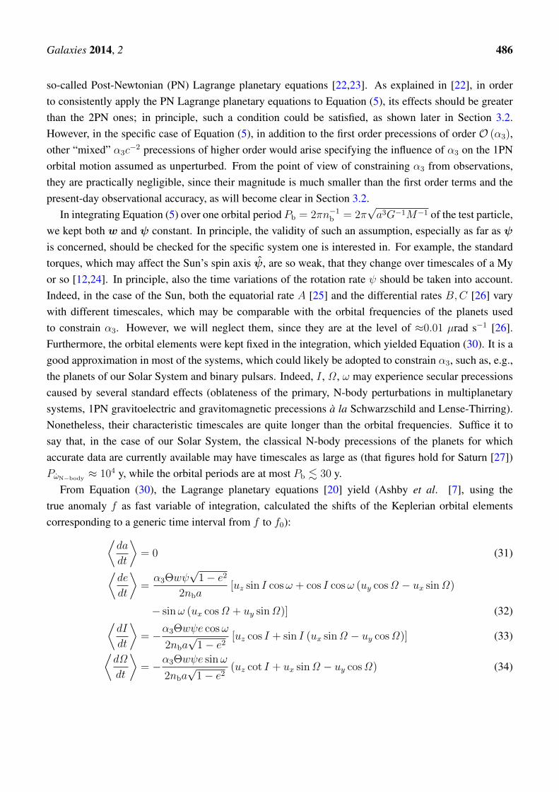
≈ 104 y, while the orbital periods are at most Pb . 30 y.From Equation (30), the Lagrange planetary equations [20] yield (Ashby et al. [7], using the

true anomaly f as fast variable of integration, calculated the shifts of the Keplerian orbital elementscorresponding to a generic time interval from f to f0):⟨

da

dt

⟩= 0 (31)⟨

de

dt

⟩=α3Θwψ

√1− e2

2nba[uz sin I cosω + cos I cosω (uy cosΩ − ux sinΩ)

− sinω (ux cosΩ + uy sinΩ)] (32)⟨dI

dt

⟩= −α3Θwψe cosω

2nba√

1− e2[uz cos I + sin I (ux sinΩ − uy cosΩ)] (33)⟨

dΩ

dt

⟩= −α3Θwψe sinω

2nba√

1− e2(uz cot I + ux sinΩ − uy cosΩ) (34)


⟨dω

dt

⟩=

α3Θwψ

2nbae√

1− e2(−1 + e2

)cosω (ux cosΩ + uy sinΩ)

+ sinω(−uy cos I cosΩ + uze

2 csc I − uz sin I + ux cos I sinΩ)

(35)⟨d$

dt

⟩=

α3Θwψ

2nbae√

1− e2(−1 + e2

)cosω (ux cosΩ + uy sinΩ)

+ sinω[−uz sin I +

(e2 − cos I

)(uy cosΩ − ux sinΩ)

+ e2uz tan

(I

2

)](36)

where the angular brackets 〈. . .〉 denote the temporal averages. It is important to note that, because ofthe factor n−1b a−1 ∝

√a in Equations (31)–(36), it turns out that the wider the system is, the larger the

effects due to α3 are. We also stress that the long-term variations of Equations (31)–(36) were obtainedwithout any a priori assumption concerning either the orbital geometry of the test particle or the spatialorientation of ψ and w. In this sense, Equations (31)–(36) are exact; due to their generality, they can beused in a variety of different specific astronomical and astrophysical systems for which accurate data areor will be available in the future.

As a further check of the validity of Equations (31)–(36), we re-obtained them by projecting theperturbing acceleration of Equation (1) onto the radial, transverse and normal directions of a trihedroncomoving with the particle and using the standard Gauss equations [20].

3. Confrontation with the Observations

3.1. Discussion of the Existing Constraints

Under certain simplifying assumptions, Will [4] used the perihelion precessions of Mercury and theEarth to infer:

|α3| . 2× 10−7 (37)

More precisely, he assumed that ψ is perpendicular to the orbital plane and used an expressionfor the precession of the longitude of perihelion$ approximated to zeroth order in e. Then, he comparedhis theoretical formulas to figures for the measured perihelion precessions, which were accurate toa ≈200–400 milliarcseconds per century (mas cty−1) level. Previous bounds inferred with the sameapproach were at the level [5]:

|α3| . 2× 10−5 (38)

A modified worst-case error analysis of simulated data of the future spacecraft-based BepiColombomission to Mercury allowed Ashby et al. [7] to infer a bound of the order of |α3| . 10−10.

Strong field constraints were obtained from the slowing down of the pulse periods of some isolatedpulsars assumed as rotating neutron stars; for an overview, see [28]. In particular, Will [4], from theimpact of Equation (1) on the rotation rate of the neutron stars and using statistical arguments concerningthe randomness of the orientation of the pulsars’ spins, inferred:

|α3| ≤ 2× 10−10 (39)


where α3 is the strong field equivalent of the conservation-law/preferred-frame PPN parameter. Thisapproach was followed by Bell [29] with a set of millisecond pulsars obtaining [29,30]:

|α3| . 10−15 (40)

Tighter bounds on |α3|were put from wide-orbit binary millisecond pulsars, as well [28]. They rely uponthe formalism of the time-dependent eccentricity vector e(t) = eF+eR(t) by Damour and Schaefer [31],where eR(t) is the part of the eccentricity vector rotating due to the periastron precession, while eF isthe forced component. Wex [32] inferred:

|α3| ≤ 1.5× 10−19 (41)

at the 95% confidence level, while Stairs et al. [33] obtained:

|α3| ≤ 4× 10−20 (42)

at the 95% confidence level. Such strong-field constraints are much tighter than the weak-field ones byWill [4]. Nonetheless, it is important to stress that their validity should not be straightforwardlyextrapolated to the weak-field regime for the reasons discussed in [15], contrary to what is often done inthe literature (see, e.g., [7]). More specifically, Shao and Wex [15] warn that it is always recommendableto specify the particular binary system used to infer the given constraints. Indeed, using differentpulsars implies a potential compactness-dependence (or mass-dependence) because of certain peculiarphenomena, such as spontaneous scalarization [34], which may take place. Moreover, they heavily relyupon statistical considerations to cope with the partial knowledge of some key systems’ parameters, suchas the longitude of the ascending nodes and the pulsars’ spin axes. Furthermore, the inclinations are ofteneither unknown or sometimes determined modulo the ambiguity of I → 180 − I . Finally, assumptionson the evolutionary history of the systems considered come into play, as well.

A general remark valid for almost all of the upper bounds on α3/α3 just reviewed is, now, inorder before offering to the reader our own ones. We stress that the following arguments are notlimited merely to the PPN parameter considered in this study, being, instead, applicable to othernon-standard (with such a denomination, we refer to any possible dynamical feature of motion, includedin the PPN formalism or not, departing from general relativity) effects, as well. Strictly speaking,the tests existing in the literature did not yield genuine “constraints” on either α3 or its strong-fieldversion α3. Indeed, they were never explicitly determined in a least square sense as solved-forparameters in dedicated analyses in which ad hoc modified models including their effects were fit toobservations. Instead, a somewhat “opportunistic” and indirect approach has always been adopted, sofar, by exploiting already existing observation-based determinations of some quantities, such as, e.g.,perihelion precessions, pulsar spin period derivatives, etc. Theoretical predictions for α3-driven effectswere, then, compared with more or less elaborated arguments to such observation-based quantities toinfer the bounds previously quoted. In the aforementioned sense, they should rather be seen as anindication of acceptable values. For example, think about the pulsar spin period derivative due toα3 [4]. In [28], it is possible to read: “Young pulsars in the field of the Galaxy [. . . ] all show positiveperiod derivatives, typically around 10−14 s/s. Thus, the maximum possible contribution from α3 mustalso be considered to be of this size, and the limit is given by α3 < 2 × 10−10 [4]”. In principle, a


putative unmodeled signature, such as the one due to α3/α3, could be removed to some extent in thedata reduction procedure, being partly “absorbed” in the estimated values of other explicitly solved-forparameters. That is, there could be still room, in principle, for larger values of the parameters of theunmodeled effect one is interested in with respect to their upper bounds, indirectly inferred as previouslyoutlined. On the other hand, it must also be remarked that, even in a formal covariance analysis, there isthe lingering possibility that some still unmodeled/exotic competing physical phenomenon, not evenconceived, may somewhat lurk in the explicitly estimated parameters of interest. Another possibledrawback of the indirect approach could consist in that one looks at just one PPN parameter at a time, bymore or less tacitly assuming that all of the other ones are set to their standard general relativistic values.This fact would drastically limit the meaningfulness of the resulting bounds, especially when it seemsunlikely that other parameters, closely related to the one that is allowed to depart from its standard value,can, instead, simultaneously assume just their general relativistic values. It may be the case here withα3 and, e.g., the other Lorentz-violating preferred-frame PPN parameters α1, α2. Actually, even in a fullcovariance analysis targeted to a specific effect, it is not conceivable to estimate all of the parameters onewants; a compromise is always necessarily implemented by making a selection of the parameters, whichcan be practically determined. However, in Section 3.2, we will show how to cope with such an issue inthe case of the preferred-frame parameters α1, α2, α3 by suitably using the planetary perihelia. Moreover,the upper bounds coming from the aforementioned “opportunistic” approach should not be consideredas unrealistically tight, because they were obtained in a worst possible case, i.e., by attributing to theunmodeled effect of interest the whole experimental range of variation of the observationally determinedquantities used. Last, but not least, at present, it seems unlikely, although certainly desirable, that theastronomers will reprocess observational data records several decades long by purposely modifying theirmodels to include this or that non-standard effect every time.

The previous considerations should be kept in mind in evaluating the bounds on α3 offered in thenext Sections.

3.2. Preliminary Upper Bounds From the Planetary Perihelion Precessions

Pitjeva [35] recently processed a huge observational data set of about 680,000 positionalmeasurements for the major bodies of the Solar System spanning almost one century (1913–2011) byfitting an almost complete suite of standard models to the observations. They include all the knownNewtonian and Einsteinian effects for measurements, propagation of electromagnetic waves and bodies’orbital dynamics up to the 1PN level, with the exception of the gravitomagnetic field of the rotatingSun. Its impact, which is negligible in the present context, is discussed in the text. In one of theglobal solutions produced, Pitjeva and Pitjev [36] kept all of the PPN parameters fixed to their generalrelativistic values and, among other things, estimated corrections ∆$ to the standard (i.e., Newtonianand Einsteinian) perihelion precessions of some planets: they are quoted in Table 1.

By construction, they account, in principle, for any mismodeled/unmodeled dynamical effect, alongwith some mismodeling of the astrometric and tracking data; thus, they are potentially suitable toput preliminary upper bounds on α3 by comparing them with Equation (36). See Section 3.1 for adiscussion on potential limitations and strength of such an indirect, opportunistic approach. We stress


once again that an examination of the existing literature shows that such a strategy is widely adoptedfor preliminarily constraining several non-standard effects in the Solar System; see, e.g., the recentworks [37–41]. Here, we recall that, strictly speaking, it allows one to test alternative theories of gravitydiffering from general relativity just for α3, all of the other PPN parameters being set to their generalrelativistic values. If and when the astronomers will include α3 in their dynamical models, then it couldbe simultaneously estimated along with a selection of other PPN parameters. Similar views can be foundin [42].

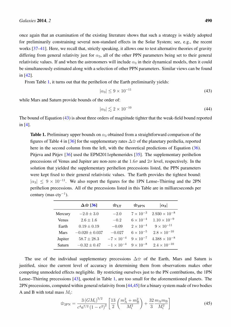
From Table 1, it turns out that the perihelion of the Earth preliminarily yields:

|α3| ≤ 9× 10−11 (43)

while Mars and Saturn provide bounds of the order of:

|α3| . 2× 10−10 (44)

The bound of Equation (43) is about three orders of magnitude tighter that the weak-field bound reportedin [4].

Table 1. Preliminary upper bounds on α3 obtained from a straightforward comparison of thefigures of Table 4 in [36] for the supplementary rates ∆$ of the planetary perihelia, reportedhere in the second column from the left, with the theoretical predictions of Equation (36).Pitjeva and Pitjev [36] used the EPM2011ephemerides [35]. The supplementary perihelionprecessions of Venus and Jupiter are non-zero at the 1.6σ and 2σ level, respectively. In thesolution that yielded the supplementary perihelion precessions listed, the PPN parameterswere kept fixed to their general relativistic values. The Earth provides the tightest bound:|α3| ≤ 9 × 10−11. We also report the figures for the 1PN Lense–Thirring and the 2PNperihelion precessions. All of the precessions listed in this Table are in milliarcseconds percentury (mas cty−1).

∆$ [36] $LT $2PN |α3|

Mercury −2.0± 3.0 −2.0 7× 10−3 2.930× 10−8

Venus 2.6± 1.6 −0.2 6× 10−4 1.10× 10−9

Earth 0.19± 0.19 −0.09 2× 10−4 9× 10−11

Mars −0.020± 0.037 −0.027 6× 10−5 2.8× 10−10

Jupiter 58.7± 28.3 −7× 10−4 9× 10−7 4.388× 10−8

Saturn −0.32± 0.47 −1× 10−4 9× 10−8 2.4× 10−10

The use of the individual supplementary precessions ∆$ of the Earth, Mars and Saturn isjustified, since the current level of accuracy in determining them from observations makes othercompeting unmodeled effects negligible. By restricting ourselves just to the PN contributions, the 1PNLense–Thirring precessions [43], quoted in Table 1, are too small for the aforementioned planets. The2PN precessions, computed within general relativity from [44,45] for a binary system made of two bodiesA and B with total mass Mt:

$2PN =3 (GMt)

5/2

c4a7/2 (1− e2)2

[13

2

(m2

A +m2B

M2t

)+

32

3

mAmB

M2t

](45)


are completely negligible (see Table 1). As remarked in Section 3.1, the assumption that the otherpreferred-frame PPN parameters α1, α2 are zero when a non-zero value for α3 is admitted seems unlikely.The availability of more than one perihelion extra-precession ∆$ allows us to cope with such an issue.Indeed, it is possible to simultaneously infer bounds on α1, α2, α3, which are, by construction, mutuallyindependent of each other. From the following linear system of three equations in the three unknownsα1, α2, α3:

∆$j = α1$j.α1

+ α2$j.α2

+ α3$j.α3, j = Earth, Mars, Saturn (46)

where the coefficients $.α1 , $.α2 , $.α3 are the analytical expressions of the pericenter precessions (as faras α3 is concerned, $.α3 comes from Equation (35), while $.α1 , $.α2 can be found in [46]) caused byα1, α2, α3, and by using the figures in Table 1 for ∆$j , one gets:

α1 = (−2± 2)× 10−6 (47)

α2 = (3± 4)× 10−6 (48)

α3 = (−4± 6)× 10−10 (49)

It can be noticed that the bound on α3 of Equation (49) is slightly weaker than the ones listed inTable 1, obtained individually from each planet; nonetheless, it is free from any potential correlationwith α1, α2. It is also interesting to notice how the bounds on α1, α2 of Equations (47) and (48) aresimilar, or even better in the case of α2, than those inferred in [46] in which the INPOP10aephemerideswere used [47]. In it, all of the rocky planets of the Solar System were used to separate (the α1, α2

planetary signals are enhanced for close orbits) α1, α2 from the effects due to the unmodeled Sun’sgravitomagnetic field and the mismodeled solar quadrupole mass moment, which have an impact onMercury and, to a lesser extent, Venus. Interestingly, our bounds on α3 of Equations (43), (44) and (49)are roughly of the same order of magnitude of the expected constraint from BepiColombo [7]; the sameholds also for Equations (47) and (48). We remark that the approach of Equation (46) can, in principle,be extended also to other planets and/or other orbital elements, such as the nodes [47], to separate morePPN parameters and other putative exotic effects. To this aim, it is desirable that the astronomers willrelease corrections to the standard precessions of more orbital elements for an increasing number ofplanets in future global solutions.

It may be worthwhile noticing from Table 1 that Pitjeva and Pitjev [36] obtained marginally significantnon-zero precessions for Venus and Jupiter. They could be used to test the hypothesis that α3 6= 0 bytaking their ratio and confronting it with the corresponding theoretical ratio, which, for planets of thesame central body, such as the Sun, is independent of α3 itself. From Table 1 and Equation (36), it is:

∆$Ven

∆$Jup

= 0.044± 0.034 (50)

$Venα3

$Jupα3

= 2.251 (51)

Thus, the existence of the α3-induced precessions would be ruled out, independently of the value of α3

itself. However, caution is in order in accepting the current non-zero precessions of Venus and Jupiter asreal; further independent analyses by astronomers are required to confirm or disproof them as genuinephysical effects needing explanation.


Finally, we mention that the use of the supplementary perihelion precessions determined by Fiengaet al. with the INPOP10a ephemerides [47] would yield less tight bounds on |α3|, because of the loweraccuracy of the INPOP10a-based ∆$ with respect to those determined in [36] by a factor ≈ 1.4 − 4

for the planets used here. More recent versions of the INPOP ephemerides, i.e., INPOP10e [48] andINPOP13a [49], have been recently produced, but no supplementary orbital precessions have yet beenreleased for them.

4. Summary and Conclusions

In this paper, we focused on the Lorentz invariance/momentum-conservation PPN parameter α3 andon some of its orbital effects.

We analytically calculated the long-term variations of the standard Keplerian orbital elements of a testparticle orbiting a compact primary. Our results are exact in the sense that we did not restrict ourselvesto any a priori peculiar orientation of the primary’s spin axis. Furthermore, the orbital geometry of thenon-compact object was left unconstrained in our calculations. Thus, they have a general validity, whichmay allow one to use them in different astronomical and astrophysical scenarios.

We used the latest results in the field of the planetary ephemerides of the Solar System to preliminarilyinfer new weak-field bounds on α3. From a linear combination of the current constraints on possibleanomalous perihelion precessions of the Earth, Mars and Saturn, recently determined with the EPM2011ephemerides in global solutions in which all of the PPN parameters were kept fixed to their standardgeneral relativistic values, we preliminarily inferred |α3| ≤ 6× 10−10. It is about three orders ofmagnitude better than previous weak-field constraints existing in the literature. Slightly less accuratebounds could be obtained from the supplementary perihelion precessions determined with the INPOP10aephemerides. We obtained our limit on α3 by allowing also for possible non-zero values of the otherpreferred-frame PPN parameter α1, α2, for which we got α1 ≤ 2 × 10−6, α2 ≤ 4 × 10−6. All suchbounds, by construction, are mutually independent of each other. An alternative strategy, requiringdedicated and time-consuming efforts, would consist in explicitly modeling the effects accounted for byα3 (and, possibly, by other PPN parameters, as well) and re-processing the same planetary data set withsuch ad hoc modified dynamical models to estimate α3 along with other selected parameters in dedicatedcovariance analyses.

Conflicts of Interest

The authors declare no conflict of interest.

References

1. Nordtvedt, K. Equivalence Principle for Massive Bodies. II. Theory. Phys. Rev. 1968, 169,1017–1025.

2. Will, C.M. Theoretical Frameworks for Testing Relativistic Gravity. II. ParametrizedPost-Newtonian Hydrodynamics, and the Nordtvedt Effect. Astrophys. J. 1971, 163, 611–628.


3. Will, C.M.; Nordtvedt, K., Jr. Conservation Laws and Preferred Frames in Relativistic Gravity.I. Preferred-Frame Theories and an Extended PPN Formalism. Astrophys. J. 1972, 177, 757–774.

4. Will, C.M. Theory and Experiment in Gravitational Physics; Cambridge University Press:Cambridge, UK, 1993.

5. Nordtvedt, K., Jr.; Will, C.M. Conservation Laws and Preferred Frames in Relativistic Gravity.II. Experimental Evidence to Rule Out Preferred-Frame Theories of Gravity. Astrophys. J. 1972,177, 775–792.

6. Nordtvedt, K. Post-Newtonian Gravitational Effects in Lunar Laser Ranging. Phys. Rev. D 1973,7, 2347–2356.

7. Ashby, N.; Bender, P.L.; Wahr, J.M. Future gravitational physics tests from ranging to theBepiColombo Mercury planetary orbiter. Phys. Rev. D 2007, 75, 022001.

8. Turyshev, S.G. Experimental Tests of General Relativity. Annu. Rev. Nucl. Part. Sci. 2008, 58,207–248.

9. Seidelmann, P.K.; Archinal, B.A.; A’Hearn, M.F.; Conrad, A.; Consolmagno, G.J.; Hestroffer, D.;Hilton, J.L.; Krasinsky, G.A.; Neumann, G.; Oberst, J.; et al. Report of the IAU/IAG WorkingGroup on cartographic coordinates and rotational elements: 2006. Celest. Mech. Dyn. Astron.2007, 98, 155–180.

10. Warburton, R.J.; Goodkind, J.M. Search for evidence of a preferred reference frame. Astrophys. J.1976, 208, 881–886.

11. Hellings, R.W. Testing Relativity with Solar System Dynamics. In General Relativity andGravitation Conference; Bertotti, B., de Felice, F., Pascolini, A., Eds.; Reidel: Dordrecht,The Netherland, 1984; pp. 365–385.

12. Nordtvedt, K. Probing gravity to the second post-Newtonian order and to one part in 10 to the 7thusing the spin axis of the sun. Astrophys. J. 1987, 320, 871–874.

13. Damour, T.; Esposito-Farèse, G. Testing local Lorentz invariance of gravity with binary-pulsardata. Phys. Rev. D 1992, 46, 4128–4132.

14. Damour, T.; Esposito-Farèse, G. Testing for preferred-frame effects in gravity with artificial Earthsatellites. Phys. Rev. D 1994, 49, 1693–1706.

15. Shao, L.; Wex, N. New tests of local Lorentz invariance of gravity with small-eccentricity binarypulsars. Class. Quantum Grav. 2012, 29, 215018.

16. Hinshaw, G.; Weiland, J.L.; Hill, R.S.; Odegard, N.; Larson, D.; Bennett, C.L.; Dunkley, J.;Gold, B.; Greason, M.R.; Jarosik, N.; et al. Five-Year Wilkinson Microwave Anisotropy ProbeObservations: Data Processing, Sky Maps, and Basic Results. Astrophys. J. Suppl. Ser. 2009,180, 225–245.

17. Beck, J.G. A comparison of differential rotation measurements—(Invited Review). Sol. Phys.2000, 191, 47–70.

18. Snodgrass, H.B.; Ulrich, R.K. Rotation of Doppler features in the solar photosphere. Astrophys. J.1990, 351, 309–316.

19. Ulrich, R.K. The influence of partial ionization and scattering states on the solar interior structure.Astrophys. J. 1982, 258, 404–413.


20. Bertotti, B.; Farinella, P.; Vokrouhlický, D. Physics of the Solar System; Kluwer Academic Press:Dordrecht, The Netherland, 2003.

21. Kopeikin, S.; Efroimsky, M.; Kaplan, G. Relativistic Celestial Mechanics of the Solar System;Wiley-VCH: Berlin, Germany, 2011.

22. Calura, M.; Fortini, P.; Montanari, E. Post-Newtonian Lagrangian planetary equations. Phys.Rev. D 1997, 56, 4782–4788.

23. Calura, M.; Montanari, E.; Fortini, P. Lagrangian planetary equations in Schwarzschild spacetime.Class. Quantum Gravity 1998, 15, 3121–3129.

24. Souami, D.; Souchay, J. The solar system’s invariable plane. Astron. Astrophys. 2012, 543, A133.25. Javaraiah, J. A Comparison of Solar Cycle Variations in the Equatorial Rotation Rates of the

Sun’s Subsurface, Surface, Corona, and Sunspot Groups. Sol. Phys. 2013, 287, 197–214.26. Javaraiah, J. Long-Term Variations in the Solar Differential Rotation. Sol. Phys. 2003, 212,

23–49.27. Database. Available online: http://ssd.jpl.nasa.gov/txt/p_elem_t2.txt (accessed on 22

September 2014).28. Stairs, I.H. Testing General Relativity with Pulsar Timing. Living Rev. Relat. 2003, 6,

doi:10.12942/lrr-2003-5.29. Bell, J.F. A Tighter Constraint on Post-Newtonian Gravity Using Millisecond Pulsars.

Astrophys. J. 1996, 462, 287.30. Bell, J.F.; Damour, T. A new test of conservation laws and Lorentz invariance in relativistic

gravity. Class. Quantum Gravity 1996, 13, 3121–3127.31. Damour, T.; Schaefer, G. New tests of the strong equivalence principle using binary-pulsar data.

Phys. Rev. Lett. 1991, 66, 2549–2552.32. Wex, N. Small-eccentricity binary pulsars and relativistic gravity. In Proceedings of the 177th

Colloquium of the IAU, Bonn, Germany, 30 August–3 September 1999.33. Stairs, I.H.; Faulkner, A.J.; Lyne, A.G.; Kramer, M.; Lorimer, D.R.; McLaughlin, M.A.;

Manchester, R.N.; Hobbs, G.B.; Camilo, F.; Possenti, A.; et al. Discovery of Three Wide-OrbitBinary Pulsars: Implications for Binary Evolution and Equivalence Principles. Astrophys. J.2005, 632, 1060–1068.

34. Damour, T.; Esposito-Farèse, G. Nonperturbative strong-field effects in tensor-scalar theories ofgravitation. Phys. Rev. Lett. 1993, 70, 2220–2223.

35. Pitjeva, E.V. Updated IAA RAS Planetary Ephemerides-EPM2011 and Their Use in ScientificResearch. Sol. Syst. Res. 2013, 47, 386–402.

36. Pitjeva, E.V.; Pitjev, N.P. Relativistic effects and dark matter in the Solar system from observationsof planets and spacecraft. Mon. Not. R. Astron. Soc. 2013, 432, 3431–3437.

37. Avalos-Vargas, A.; Ares de Parga, G. The precession of the orbit of a charged body interactingwith a massive charged body in General Relativity. Eur. Phys. J. Plus 2012, 127, 155.

38. Xie, Y.; Deng, X.M. f(T ) gravity: Effects on astronomical observations and Solar systemexperiments and upper bounds. Mon. Not. R. Astron. Soc. 2013, 433, 3584–3589.

39. Cheung, Y.K.E.; Xu, F. Constraining the String Gauge Field by Galaxy Rotation Curves andPerihelion Precession of Planets. Astrophys. J. 2013, 774, 65.


40. Deng, X.M.; Xie, Y. Preliminary limits on a logarithmic correction to the Newtonian gravitationalpotential in the solar system. Astrophys. Space Sci. 2013, 350, 103–107.

41. Li, Z.W.; Yuan, S.F.; Lu, C.; Xie, Y. New upper limits on deviation from the inverse-squarelaw of gravity in the solar system: A Yukawa parameterization. Res. Astron. Astrophys. 2014,14, 139–143.

42. Nordtvedt, K. Improving gravity theory tests with solar system “grand fits”. Phys. Rev. D 2000,61, 122001.

43. Lense, J.; Thirring, H. Über den Einfluß der Eigenrotation der Zentralkörper auf die Bewegungder Planeten und Monde nach der Einsteinschen Gravitationstheorie. Physikalische Zeitschrift1918, 19, 156–163. (In German)

44. Damour, T.; Schafer, G. Higher-order relativistic periastron advances and binary pulsars. NuovoCimento B 1988, 101, 127–176.

45. Wex, N. The second post-Newtonian motion of compact binary-star systems with spin. Class.Quantum Gravity 1995, 12, 983–1005.

46. Iorio, L. Constraints on the Preferred-Frame α1, α2 Parameters from Solar System PlanetaryPrecessions. Int. J. Mod. Phys. D 2014, 23, 1450006.

47. Fienga, A.; Laskar, J.; Kuchynka, P.; Manche, H.; Desvignes, G.; Gastineau, M.; Cognard, I.;Theureau, G. The INPOP10a planetary ephemeris and its applications in fundamental physics.Celest. Mech. Dyn. Astron. 2011, 111, 363–385.

48. Fienga, A.; Manche, H.; Laskar, J.; Gastineau, M.; Verma, A. INPOP new release: INPOP10e.2013, arXiv:1301.1510.

49. Verma, A.K.; Fienga, A.; Laskar, J.; Manche, H.; Gastineau, M. Use of MESSENGERradioscience data to improve planetary ephemeris and to test general relativity. Astron. Astrophys.2014, 561, A115.

c© 2014 by the author; licensee MDPI, Basel, Switzerland. This article is an open access articledistributed under the terms and conditions of the Creative Commons Attribution license(http://creativecommons.org/licenses/by/4.0/).

Orbital Motions and the Conservation-Law/Preferred-Frame α3 Parameter

Documents

Transcript of Orbital Motions and the Conservation-Law/Preferred-Frame α3 Parameter