Pergamon Bulletin of Mathematical Biology Vol. 56, No. 3, pp. 562586, 1994

Copyright © 1994 Elsevier Science Ltd Printed in Great Britain. All rights reserved

0092-8240/94 $7.00 + 0.00

N U M E R I C A L S I M U L A T I O N O F P R O P A G A T I N G C O N C E N T R A T I O N P R O F I L E S I N R E N A L T U B U L E S

• E. BRUCE PITMAN Department of Mathematics, State University of New York, Buffalo, NY 14214-3093, U.S.A.

(E.mail: pitman@galileo.math.buffalo.edu )

• H . E . LAYTON

Department of Mathematics, Duke University, Box 90320, Durham, NC 27708-0320, U.S.A.

(E.mail: layton@math.duke.edu)

• LEON C. MOORE

Department of Physiology and Biophysics, State University of New York, Stony Brook, NY 11794, U.S.A.

(E.mail: moore@pofvax.pnb.sunysb.edu)

Method-dependent mechanisms that may affect dynamic numerical solutions of a hyperbolic partial differential equation that models concentration profiles in renal tubules are described. Some numerical methods that have been applied to the equation are summarized, and ways by which the methods may misrepresent true solutions are analysed. Comparison of these methods demonstrates the need for thoughtful application of computational mathematics when simulating complicated time-dependent phenomena.

Introduction. Mathematical modeling of flow in renal tubules has played an important role in elucidating the urine concentrating mechanism and the tubuloglomerular feedback (TGF) system (Holstein-Rathlou and Marsh, 1990; Layton et al., 1991; Stephenson, 1992). An element common to many dynamic models of intratubular flow is a hyperbolic partial differential equation (PDE) expressing solute conservation in fluid flowing through a rigid tubule of small diameter. The solution to this PDE expresses luminal solute concentration as a function of time and axial position along the tube. Owing to the presence of nonlinearities, the PDE must be solved numerically.

The purpose of this paper is to demonstrate that care must be taken in choosing a numerical method (or "scheme"); for the PDE, to ensure that the

567

568 E B. PITMAN et aL

computed solution is in acceptable agreement with the actual solution. First we summarize some of the schemes available for solving a: simplified version of this PDE, and then we consider the suitability of the schemes for representing concentration profiles. We apply the schemes to a simplified form of the PDE, provide examples of the ways in which the schemes misrepresent the actual solutions, and describe the theoretical basis for the numerical artifacts responsible for the misrepresentations. Although our analysis contains no new theoretical results, it does provide a unified exposition of some applicable methods in the context of renal modeling.

The Model Equation. In a companion paper (Layton and Pitman, 1994), we derive, by enforcing solute balance, the hyperbolic PDE typically used to represent the solute concentration in a renal tubule. That PDE, obtained under the assumption that axial convection dominates decisively over diffusion, is given by:

8 1 8 1 Ot C(x, t ) - A(x) 8x [Fv(x' t)C(x, t)] +. ~ Ju(x, t) (1)

where x is the axial coordinate, A(x) is the cross-sectional area of the tube atx , C(x, t) is intratubular solute concentration at x at time t, Fv(X, t) is intratubular water flow, and Ju(x, t) is flux of solute into the tube through the tubular walls.

Observe that ~ is proportional to the circumference of the tube. In this equation every quantity is expressed in nondimensional form, following the convention in Layton and Pitman (1994).

In models of renal tubules the walls are often assumed to be water-permeable with transmural water flux into the tubule given by Jr(X, t). By water Volume conservation, Jv and F v are related by:

8 Fv(X ' t). (2)

We use equation (2) and the product-rule to rewrite equation (1) as:

0 1 a5 t)= A(x) Fv( , t) c ( x , t) + - - - -

1 (J,.(x, t ) -c (x , t)Jv(x, t)). (3) ./A(x)

Here, the first term on the right-hand side represents the effect on concentration that arises from axial solute convection at flow rate F v. The second term represents the effect oftransmural solute and water flux on that concentration. Observe that solute entry raises the concentration, while water entry lowers it. These transmural fluxes are referred to as "source" terms. Generally speaking,

SIMULATION o F PROPAGATING CONCENTRATION PROFILES IN TUBULES 569

the source terms depend on the both the intra- and extratubular concentrations and on the assumptions made about transmural transport.

In models of the water-impermeable ascending limb used in simulating TGF, it is assumed that Fv is independent of x, so that Jv is zero and axial flow F v is a function of time only (Holstein-Rathlou and Marsh, 1990; Layton et al., 1991).

In general, equation (3) must be solved numerically, since explicit solutions do not exist, except under very special assumptions. PDEs of this form are often solved by using an operator splitting method, in which: (1) the ordinary differential equation (ODE) obtained by disregarding the convection term is solved for one time step, to obtain a resultant concentration C*; and (2) the PDE obtained by disregarding the source terms is solved for a time step, using C* as the current concentration to be updated. To preserve second-order accuracy in time, we used a symmetric form of this splitting, introduced by Strang (1963), in solving equation (3) for mathematical simulations of TGF (Pitman and Layton, 1989; Layton et al., 1.991).

The benefit of operator splitting is that specialized methods may be applied separately to the PDE and to the ODE. Scientific understanding of numerical methods for solving ODEs is more advanced than for solving hyperbolic PDEs, and several ODE methods are well known. Thus, we turn our attention to numerical techniques for the PDE in equation (3), without source terms. We further simplify the PDE by assuming constant axial flow rate. That is, we apply computational methods to the linear transport equation:

~t u(x, t) + a ~-x u(x, t) = 0, a>O (4)

which we obtain from equation (3) by discarding the source terms and specifying constant flow rate F v = a, and constant cross-sectional area A = 1. We also replace C by the standard dependent variable u. The action of the simplified equation is to move initial data u(x, 0) to the right at constant speed a. In the sections that follow we present several computational schemes, examine how each scheme propagates (or advects) wave profiles, and provide a Fourier analysis of the schemes. A good general reference for much of this material is by Strikwerda (1989).

Methods. We discretize, space and time with uniform space step Ax, and time step At, giving a lattice of numerical grid points. The notation u~. designates a numerical approximation to the (true) solution u at locationjAx and time nAt, i.e., uj ~ u(jAx, nat).

Given initial data u(x,O)=h(x), the solution of equation (4) is u(x, t ) = h ( x - a t ) , which may be verified by direct substitution. Along the characteristic lines in the (x, t)-plane, determined by dx/dt = a, u is constant. A

570 E.B. PITMAN et al.

reasonable computational method, then, is to differentiate in the direction that information is propagating by using a backward space difference and writing:

n + l _ _ n . . uj -us -2 (us -us_~) (5)

where 2 = aAt /Ax is known as the Courant-Friedrichs-Lewy number (or the CFL number). This scheme, called "upwind differencing", is only first-order accurate in space and time, but it can be shown to preserve monotonicity (Godunov, 1959). That is, when a consecutive set of increasing (or decreasing) grid values is advected by this scheme, the resulting grid values are again increasing (or decreasing). The upwind scheme is stable for 2 ~< 1. This criterion has a physically plausible interpretation: for if aAt > Ax, the difference quotient (u s -u~_ ~)/Ax is based on information that has propagated past the location jAx .

To achieve second-order accuracy, Lax and Wendroff (1960) began with the Taylor series approximation:

U . + I n n ( A t ) 2

s =uj +(ut) 7 At+(u,,)s 2 (6)

where u t = ~?u/Ot. Next, using the PDE, they replaced the time derivatives with space derivatives; thus, by equation (4):

u t = - a u x and u t t = ( u , ) , = ( - - a u x ) t = - a ( u t ) ~ = a Z u x , . (7)

Finally they replaced space derivatives with centered-difference approxima- tions. The resulting scheme may be written:

22 . + 1 . 2 . - u " " - 2 u ] + " ). (8)

b/j : l / j - - ~ (/./j +1 j - 1 ) "1- y (/'/j +1 /A j_ I

The Lax-Wendroff scheme is second-order accurate in space and time and stable for 2 ~< 1, but does not preserve monotonicity. [Godunov (1959) showed that a monotonicity-preserving difference scheme that depends linearly on the grid values is at most first-order accurate.]

The scheme we have used in simulations of TGF combines the upwind and Lax-Wendroff schemes (Pitman and Layton, 1989; Layton et al., 1991). Written explicitly, the scheme is:

.+1 . / 22 2-2 2 ) /

+ ( 1 - , ~ ) ( - ~ " " u" tuj - j _ 1))- (9 )

When @~. = 1 the scheme uses Lax-Wendroff differencing; when 0~.=0, the

S I M U L A T I O N O F P R O P A G A T I N G C O N C E N T R A T I O N P R O F I L E S I N T U B U L E S 571

scheme reverts to upwind differencing. This scheme may be rewritten and conceptualized as a weighted sum of two numerical fluxes: a high-order flux Ha+ 1/2 and a low-order flux L ] + I / 2 . That is:

n + l n n n uj -u j - - (F j+ l /2 -F}_1 /2 ) (10)

where the composite numerical flux is:

with

?l t l ?1 ?~ ?l F~+ 1/2 = ~)jH}+ 1/2 "~ (1 - - @j)Lj+ 1/2 (11)

H]+1/2 2 , +u~) 22 %+1 - 2 (u7+1- 7) and LT+l/2=2u (12)

When @~ = 1 (the Lax-Wendroff case), the scheme has second-order accuracy in space and time. However, the limiter (I)~ is designed to adjust the contribution of the Lax-Wendroff flux to preserve monotonicity. In particular, as is evident below, any monotonicity-preserving scheme reverts to upwinding at local extrema. Thus, at some points in space and at some times, this scheme may be only first-order accurate locally. But if these points constitute a small subset of (x, t)-space, the cumulative effect is that the scheme will exhibit second-order accuracy.

A class of numerical methods called flux-limiting schemes can be designed by choosing the limiter to depend on local gradients: @~=f(rT) where r~=

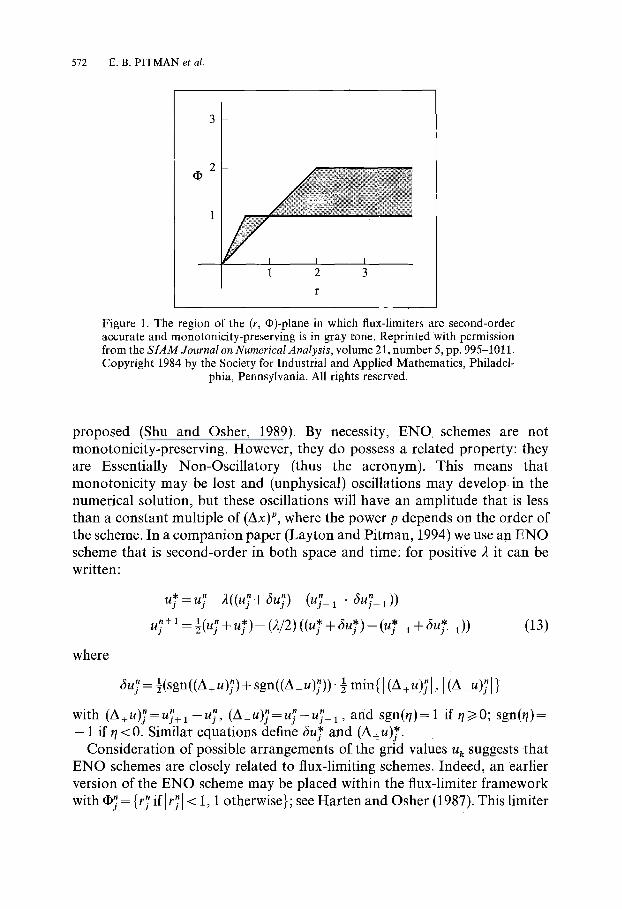
/An __ u n n j j_l) /(Uj+l-u~). Zalesak (1987) tested some important limiters, and Sweby (1984) formulated principles for selecting good limiters. In particular, Sweby showed that in the region of (r, @)-space shown in Fig. 1, second-order accuracy and monotonicity can be attained. Using his principle, two frequently used limiters are:

• MUSCL (Monotone Upstream-centered Scheme for Conservation Laws):

@~ = max(0, min(2, 2r7, (1 + r~)/2))

• and Min-Mod (Minimum Modulus):

q)~. = max(0, min(1, rT) ).

We used the MUSCL limiter in Layton e t al. (1991) and the Min-Mod limiter in Pitman and Layton (1989). When solving equations for which the flow rate can switch from positive to negative, the flux-limiter formulation given above must be modified.

A related class of methods, called ENO schemes, has been designed in an attempt to maintain high-order accuracy everywhere (Harten and Osher, 1987). ENO schemes of second-, third-, and fourth-order accuracy have been

572 E.B. PITMAN et al.

0

N. =

F I I I 1 2 3

Figure 1. The region of the (r, ~)-plane in which flux-limiters are second-order accurate and monotonicity-preserving is in gray tone. Reprinted with permission from the S I A M Journal on Numerical Analysis , volume 21, number 5, pp. 995-1011. Copyright 1984 by the Society for Industrial and Applied Mathematics, Philadel-

phia, Pennsylvania. All rights reserved.

proposed (Shu and Osher, 1989). By necessity, ENO. schemes are not monotonicity-preserving. However, they do possess a related property: they are Essentially Non-Oscillatory (thus the acronym). This means that monotonicity may be lost and (unphysical) oscillations may develop-in the numerical solution, but these oscillations will have an amplitude that is less than a constant multiple of (Ax) p, where the power p depends on the order of the scheme. In a companion paper (Layton and Pitman, 1994) we use an ENO scheme that is second-order in both space and time: for positive 2 it can be written:

where

= " u" + 5 u 7 1)) n + l 1 n , uj (13)

6u~. = ½(sgn( (A + u);) + sgn((A_ u);)) - ½ min( [ (A + u)j' [, I (A_ u)y I }

( A . xn /An n 12 n n n with ~ + u S = j + l - U j , ( A _ ) ; - u j - u ; _ 1, and sgn(t/)=l if t/~>0; sgn(t/)= - 1 if 77 < 0. Similar equations define 6u* and (A_+ u)*.

Consideration of possible arrangements of the grid values u k suggests that ENO schemes are closely related to flux-limiting schemes. Indeed, an earlier version of the ENO scheme may be placed within the flux-limiter framework with 07= {r~. i f l r ] l < 1, 1 otherwise}; see Harten and Osher (1987). This limiter

SIMULATION OF PROPAGATING CONCENTRATION PROFILES IN TUBULES 573

falls outside the monotonicity-preserving region if r~ < 0, and is equivalent to the M i n - M o d limiter if r~ > 0.

A different type of second-order scheme may be obtained by using differences in space and time centered at grid midpoints. This differencing for u t and u x is defined by letting:

1 "+'-u" t l j - - l l 2 - - 2 a t t u j - 1 j - - l ) )

1 . "~n+1/2 _ _ ( ( U j + l . n + l , n n uxjj- 1/2 2 Ax - u j_ 1 ) + (uj - u j_ 1 ))- (14)

By substituting these expressions into equation (4) one obtains:

-"+l"'-£)=u;(1-A)+u7 1(1 +R). "+1(1 + 2)-}-uj_ 1 t l uj (15)

This scheme, similar to the Crank-Nicholson (CN) scheme used for parabolic PDEs, is sometimes called the "box" scheme [-see von Rosenberg (1969), pp. 34-37]. It has been used in a numerical simulation of T G F (Holstein- Rathlou and Marsh, 1990). By Godunov's result, the CN scheme cannot be monotonicity-preserving. The E N O and CN schemes, like the flux-limiting schemes, must be modified if the flow rate is allowed to change sign.

Propagation Examples. To better understand the properties of the schemes introduced in the previous section we illustrate, by numerical experiment, some ways in which the schemes produce distorted solutions when used to advect simple waveforms. To show the extremes of behavior we mostly compare the more recently developed MUSCL scheme with the more traditional CN scheme. In the subsequent section we use the Fourier transform to better understand the results.

Given a waveform w(x) we define a function h(x) by:

i x<0 .1 h(x)= (x) 0 . 1 < x < 0 . 5 . (16)

0 . 5 < x

We solve equation (4) on the interval x e [0, 2], with a = 1 and initial data u(x, O)= h(x). At the boundary x = 0, u is set to zero. In Figs 2-5 we plot, for time t = 1, the exact solution with a thin solid curve and the numerical solution with thick dashes. For all numerical tests, the space grid is Ax = 1/100.

In Fig. 2a,b, the original square pulse h, obtained with w = 0.25, has been propagated by one unit in the positive x-direction to give the exact solution. This exact solution has been approximated by the flux-limiting scheme with the

574 E. B, P I T M A N et al.

0.3

0.2

0.1

0.0

I

Exact

------ F CT

-0,] i

0 .0 0.5

I I

1.0 1.5

X

(a)

2.0

0.3

0.2

0.1

0.0

-0.1 0.0

- - Exact

- - - - C N

r r

0.5 1.0

X

I I

(b)

, I r"'r'Y 1.5 2.0

Figure 2_ Comparison of the (a) flux-limiting and (b) CN scheme in advecting a square pulse. The flux-limiting scheme is designated by the acronym FTC here and in subsequent figures. Here, and in Figs 3-5, an initial profile given by equation (16) has been propagated to the right at speed 1 for 1 time unit. In this pair of figures, the FCT scheme produces minor rounding at the corners (evidence of dissipation), whereas the CN scheme produces spurious oscillations (evidence of dispersion).

M U S C L limiter in Fig. 2a and by the C N scheme in Fig. 2b. (The curve for the flux-limiting scheme is identified by the acronym FCT, for "flux-corrected transport", a c o m m o n synonym for flux-limited advection.) The calculations were performed with a CFL number of 2 = 0.8.

The flux-limiting scheme advects the square pulse with some rounding of the corners. Roughly speaking, this exemplifies a numerical error called "dissipa- tion", the smearing or smoothing out of the exact solution, possibly accompanied by a decrease in its amplitude. In contrast, the C N scheme shown in Fig. 2b introduces spurious oscillations that extend beyond the region delineated by the exact square pulse solution. This exemplifies a numerical error called "dispersion", the decoupling of the Fourier components of the exact solution into oscillatory modes traveling at speeds different from that of the exact solution. As we show below through Fourier analysis, these results

SIMULATION OF PROPAGATING CONCENTRATION PROFILES IN TUBULES 575

0.2

0_1

0.0

-0.1

Exact ------ FCT

i

I

(a)

U -0.21 i i i

0.0 0_5 1.0 1.5 2.0 X

0.2

t i 0.1 Exact ------ CN

0.0

-0.l f

-0.2 i 0.0 0.5

i i

. ( b )

i f

1 . 0 1.5 2.0 X

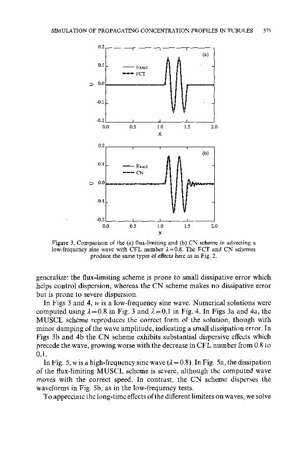
Figure 3. Comparison of the (a) flux-limiting and (b) CN scheme in advecting a low-frequency sine wave with CFL number 2=0.8. The FCT and CN schemes

produce the same types of effects here as in Fig. 2.

generalize: the flux-limiting scheme is prone to small dissipative error which helps control dispersion, whereas the CN scheme makes no dissipative error but is prone to severe dispersion.

In Figs 3 and 4, w is a low-frequency sine wave. Numerical solutions were computed using 2=0.8 in Fig. 3 and 2=0.1 in Fig. 4. In Figs 3a and 4a, the MUSCL scheme reproduces the correct form of the solution, though with minor damping of the wave amplitude, indicating a small dissipation error. In Figs 3b and 4b the CN scheme exhibits substantial dispersive effects which precede the wave, growing worse with the decrease in CFL number from 0.8 to 0.1.

In Fig. 5, w is a high-frequency sine wave (2 = 0.8). In Fig. 5a, the dissipation of the flux-limiting MUSCL scheme is severe, although the computed wave moves with the correct speed. In contrast, the CN scheme disperses the waveforms in Fig. 5b, as in the low-frequency tests.

To appreciate the long-time effects of the different limiters on waves, we solve

576 E . B . P I T M A N et al.

0.2

0.1

0.0

-0.1

Exact

- - - - - - FCT _ i

(a)

I

1,5 -0.21 I t

0.0 0.5 1.0 2_0

X

0.2

0.1

0.0

-0.1

I I

- - ExactcN J

I

(b)

A

-0.21 i i i 0.0 0.5 1.0 1.5 2.0

X

Figure 4. Comparison of the (a) flux-limiting and (b) CN scheme in advecting a low-frequency sine wave with CFL number 2 = 0.1. Note that the dispersive errors

in the CN scheme are worse than those shown in Fig. 3 for 2=0.8.

equation (4) on the unit interval with periodic boundary conditions. In Fig. 6 an initial square pulse has cycled 10 times. Figure 6a shows how the upwind scheme diffuses the pulse, the effect worsening as the CFL number decreases. Figure 6b shows the oscillatory behavior of the Lax-Wendroff scheme; although formally second-order accurate, the method produces a wildly oscillating solution. The MUSCL limiter is used in Fig. 6c, showing the important r o l e the limiter plays in providing an accurate numerical solution. The E N O scheme given by equation (13) is used in Fig. 6d. Both MUSCL and ENO diffuse the square pulse somewhat, but this diffusive effect, even at low CFL number, does not obliterate the pulse, as does upwinding. Furthermore, in contrast with the Lax-Wendroff scheme, M U S C L and ENO maintain the i n t eg r i t yo f the pulse shape. The E N O scheme shows improvement with decreasing CFL number, whereas the M U S C L scheme degrades, though both appea r to be approaching a limiting profile as the CFL approaches zero. (In Fig. 6a,c and d, the solution curves for CFL = 0.1 and CFL = 0.01 lie almost on

SIMULATION OF PROPAGATING CONCENTRATION PROFILES IN TUBULES 577

0.2

0_1

o.ol

-0.1

i [ J

(a)

_ .xact J

-0,2 I t t 0.0 0.5 1.0 1.5 2.0

X

0.2

0.I

0.0

-0.1

-O.2

0.0

b

i B m

I I I

0_5 1.0 1.5 2.0 X

Figure 5. Compar i son of the (a) flux-limiting and (b) C N scheme in advecting a high-frequency sine wave. The dissipat ion by the F C T scheme and the dispersion by the C N scheme are bo th severe, a l though the F C T solution propagates at the

correct speed.

top of each other.) In that limit, the ENO scheme appears more dissipative than the MUSCL scheme. However, the ENO scheme is easier to implement in cases where the flow rate may change sign. When used at very low CFL number, both MUSCL and ENO are well behaved.

Fourier Analysis. Insight into the origin of the numerical artifacts illustrated above can be obtained through a Fourier analysis of the difference schemes. Let vj' be a function defined on uniformly spaced points jAx of the real line. A discrete Fourier transform is defined by:

1 ~ - i,, v"(~) = ~ ,,= - ~o e aXCv~ Ax. (17)

If ~ 2 = _ ~(v,~) 2 is finite, then the Fourier transform converges and has other useful properties.

578 E. B P I T M A N et al.

I I I I

0_3 ( a )

0.2 [ . . . . - - , , ] L// ",J

O.l ........... t ' , .............

.../" / - - c ~ = o , / "--. 0 . 0 """ / - - - C F L = 0 . 1 / " -

........... C F L = 0_01

- 0 . 1 i i i i

0 . 0 0 . 2 0 . 4 0 . 6 0 . 8 1 . 0

X

I I I I

03 ad)'~\ _ . k t ~.~

0_2 - ,~ "

= o.1 I ! / 11 / - - Exact ~ ' "~"

f f / _ _ _ C F L = # ] " ~ "t 08 / ' 4 0.0 V '~ . . . . CFL = 0.1 • ~ • # -

"'~. ~ l ........... CFL = 0.01

- 0 . I v i I I i

0.0 0_2

(b)

&

k ~t

0_4 0_6 0.8 1.0

0.3

0.2

0.1

0_0

-0.1 0.0

I

(c)

Exact ~ ---CFL=08 ~

- " ~ CFL = 0.1 / %

........... CFL = 0.01

I I I 1

0.2 0.4 0.6 0_8

X

F i g u r e 6. (a) , (b ) a n d (c).

1.0

S I M U L A T I O N O F P R O P A G A T I N G C O N C E N T R A T I O N P R O F I L E S I N T U B U L E S 579

t i f I I 0.3 (d)

/ I;7 "\1 i [

| . f l ~ Exact I V \ / ,.,-'-'~ ] - - c ~ = o . 8 / \ , x

0 . 0 [-----'~-.~';" | - - - C F L = 0 . 1

-0.1 ........... CFL = 0.01

I I I I

0.0 0.2 0.4 0.6 0.8 1.0

X

Figure 6. Comparison of the (a) upwind, (b) Lax-Wendroff, (c) MUSCL, and (d) ENO schemes advecting a square pulse 10 times around the unit interval, with periodic boundary conditions. Shown are the exact solution and the solution curves produced using the different methods, for CFL numbers equal to 0.8, 0.1, and 0.01. Note that in (a), (c), and (d) the solution curves for CFL--0.1 and CFL=0.01 lie almost on top of each other. Dissipation in the upwind scheme is severe, and the Lax-Wendroff solution contains unphysical oscillations. In contrast, the FCT scheme with the MUSCL limiter reproduces the pulse with good accuacy. The ENO

scheme, closely related to the FCT scheme, also shows good performance.

The nonl inear i ty of the limiter • 7 precludes a general Four ie r analysis for a flux-limiting scheme. However , one m a y examine dispersion and dissipation for any fixed value of the limiter. Similarly, no general Four ie r analysis is possible for the E N O scheme. However , for any part icular a r rangement of the values u k, and therefore a par t icular choice of the 5us, analysis is possible. We concentrate here on the flux-limiting schemes.

Fo r fixed ~ , the t ransform of the flux-limiting scheme, equa t ion (9), is given by:

~.+ 1(~)= l + q ) ( e i ° - e - i ° ) + ~- ( e i ° - 2 + e - ' ° )

+ (1 - o ) - (18)

where 0 = Axe. After rear rangement , this equat ion can be wri t ten as:

fi" + ~(~) = g(O)O"(~) (19)

where:

g(0) -- 1 -- 2(1 - cos(0)) [1 - ~(1 -- 2)3 - i2 sin(0) (20)

580 E.B. PITMAN et al.

is known as the amplification factor. If this factor has modulus less than 1, then any error introduced in a time step is reduced during subsequent time steps, thus ensuring this scheme's numerical stability. For the flux-limiting scheme, [g]~<l if the Courant-Fr iedr ichs-Lewy condition is satisfied, that is, if 2 = a At/Ax<<. 1. If [gl= 1 there is no dissipation in the scheme and the amplitude of all Fourier modes is preserved. The amount by which ]gl is less than 1 is a measure of the scheme's dissipation.

The amplification factor for the CN scheme is:

cos2(0/2) - 22 sin2 (0/2) - 2i2 cos(0/2)sin(0/2) g(O) = cos2(0/2 ) + 22 sin2(0/2 )

(21)

It is easy to verify that [9] = 1 for all 0, independent of the CFL number 2. Thus, there is no dissipation in the CN scheme.

The transform can also be used to examine the scheme's dispersion. We return to equation (4) and take the (usual) continuous Fourier transform to obtain:

Ftt(~, t)= --i~aCt(~, t). (22)

After solving this ordinary differential equation in the variable t and evaluating at time t and t+At we find that:

fi(~, t + At) = exp(-- i~a At)fi(¢, t). (23)

This equation manifests the propagation speed a in the time update of the Fourier transform of u. [Observe that fi(~, t + A t ) a n d fi(~, t) are the exact expressions corresponding to the numerical approximations fi,+a(~) and ~"(0-]

Now write the amplification factor in equation (19) as:

g(O) = I g(O)[ exp(-- i~o~(O) At) (24)

where e(0) is the speed of propagation of a particular Fourier mode. In an ideal numerical scheme all Fourier modes would propagate with uniform speed a. However, in all real-world numerical methods, it is generally true that e(0) # a. By comparing equations (19), (23), and (24), one finds that the relative error in the propagation speed is (~(0)-a) /a .

The magnitudes of the dissipative and dispersive errors can be conveniently gauged through graphs of the amplification factor and relative propagation speed error. Figure 7a,b shows the modulus of the amplification factor [g] as a function of wave number 0 for selected CFL numbers. Figure 7a corresponds to the flux-limiting scheme in the more dissipative upwind limit, i.e., O - 0 ; Fig. 7b corresponds to the less dissipative Lax-Wendroffl imit , i.e., • - 1. Each

S I M U L A T I O N O F P R O P A G A T I N G C O N C E N T R A T I O N P R O F I L E S I N T U B U L E S 581

"6

1.00

s

0.90 ,," s

, e

0.85 s*

," CFL = 1.0 0.80 ,,' . . . . CFL = 0.5

*' . . . . . . . CFL = 0.1 0.75 , '

o

0.70 I I

-7 t /2 -7 t /4 o

0

(a)

i

i

$

i

I

~/4 ~ /2

1.00 . . . . . . . . . ~ ; . . . . .

0.95

s

0.90 *

0.85

0.80

0.75

0 . 7 0 I

- ~ / 2 - ~ / 4

. . . . . : : . ( , ; i "

C F L = 1 . 0

. . . . C F L = 0 . 5

. . . . . . . C F L = 0 . 1

I I

0 ~/4 ~/2

0

Figure 7. Dissipation error quantified through the modulus of the amplification factor 19(0)] for the (a) upwind and (b) Lax Wendrofflimits. No error corresponds

to I g(0)[= 1. Note the smaller dissipation of the Lax-Wendroff scheme.

figure provides a measure of the dissipation per timestep. For a particular CFL number, the total dissipation in a calculation for a fixed time interval accumulates according to the total number of timesteps in the interval. Thus, even though the dissipation for a single timestep at CFL = 0.1 is less than that at CFL = 0.5, the accumulated dissipation over a fixed time interval at CFL = 0.1 may exceed that at CFL--0.5 .

Figure 8a,b are the analogous plots of the dispersion error in the upwind and Lax-Wendroffl imits. Both parts of the figure show increasing dispersion as ]01 increases, For a CFL number less than 1, however, Fig. 7a,b shows increasing dissipation in both limits as 101 increases. Thus, for a CFL number less than 1, the modes that are most dispersed are also most dissipated, a convenient property that tends to damp the oscillatory numerical artifacts. This reasoning explains why dissipation only is observed in parts a of Figs 2-5.

Figure 9 shows the dispersion error for the CN scheme. (Recall that this scheme makes no dissipation error.) For 0 ~ 0, the relative error in propagation

582 E.B. PITMAN et al.

5.0 (a) F]

4°I /1 C F L = 1.0

3 . 0 . . . . c =o.5 . . . . . . . = .

1.0

o.o ...

- 1 . 0 i t

- ~ / 2 - ~ / 4 0 re /4 r t / 2

0

5.0 (b)

4.0 - - C F L = 1.0

3.0 . . . . C F L = 0.5

1.0

0.0

- 1 . 0 t t i

- 7 : / 2 - 7 t / 4 0 r~/4 re/2

0

Figure 8. Relative error in propagation speed (c~(0)- a)/a for the (a) upwind and (b) Lax-Wendrofflimits. Note that both methods are significantly dispersive, although by comparison with Fig. 7 one concludes that the modes most dispersed are also

most dissipated, especially for the upwind case_

5.0

4 .0

3.0

? ~ . ~ 2.0

1.0

0.0

-1.0

-~/2

C F L = 1.0

. . . . C F L = 0.5

S ..... , , ~ , r ~ ~ ~ ~ .-..'..". -- • -

I I I

-g/4 0 g/4

0

-~/2

Figure 9. Relative dispersion error (~(O)-a)/a for the CN scheme. Since there is no dissipation in the CN scheme, the dispersed modes maintain their amplitude.

S I M U L A T I O N OF P R O P A G A T I N G C O N C E N T R A T I O N PROFILES IN TUBULES 583

speed is always positive, indicating that all Fourier modes travel too fast. Since there is no dissipation, the speeding modes maintain their amplitude, leading to large dispersive errors. This reasoning explains the leading oscillations observed in parts b of Figs 2-5.

Application to Renal Tubules. The examples and analysis presented in the preceding sections provide insight into the behavior of some numerical schemes when they are applied to solving the constant coefficient linear advection PDE, equation (4). However, that analysis is only suggestive of the behavior obtained when the schemes are used to solve nonlinear model equations, which may include transmural transport and variable flow speeds.

We test the MUSCL and CN methods by propagating a bolus of high concentration along a model tube similar to the thick ascending limb of the nephron. (This case is of interest in the study of time-dispersal of concentration boluses in the renal medulla.) From the results for the linear equation, one expects the MUSCL scheme to smoothly propagate the concentration pulse (Figs 2-5 parts a). One also expects the CN scheme to produce a highly dispersive solution (Figs 2-5 parts b). However, the nonlinear transmural solute transport is stronger for high concentrations than for low concentra- tions, which reduces local concentration maxima and might, therefore, suppress spurious oscillations.

We numerically solve model equation (3), setting A - 1, F v =- 1, Jv = O. J~t is given by outward-directed Michaelis-Menten solute transport:

v. axC(x, t) J (x, t) = C ( x , t) + K M ' (25)

with maximum transport rate Vma x = 1 and Michaelis constant K M = 0.25. To include the source term, we used Strang splitting, as described in Pitman and Layton (1989) and Layton et al. (1991). On the interval xe[0 , 2], the initial concentration profile is given by u(x, 0) = 0.1 exp( - x) + h(x), where h(x) is the same square pulse used previously [equation (16)]. Figure 10 shows the solution curves for the MUSCL and CN schemes. As expected, the flux limiting scheme propagates the pulse smoothly, with some rounding of the corners. The CN scheme generates spurious oscillations that result in (unphysical) negative concentrations. This example suggests that the dispersive CN scheme is unsuitable for general use in models of renal tubules.

Notwithstanding the analysis and examples presented in this paper, bad dispersion or dissipation characteristics do not preclude a numerical method from yielding good results in some cases. Indeed, one motivation for this study of numerical schemes was to determine whether the CN scheme would correctly reproduce the numerical bifurcation results of Fig. 9 in Layton et al.

584 E . B . P I T M A N et al.

o3 f 0.2

0.1

0'0 /

-0.1

0.0

I I

A

FCT

------ CN

I I I

0,5 1.0 1.5 2.0

X

Figure 10. The solution curves produced by the MUSCL and CN schemes in propagating a strong pulse. The initial concentration profile was a decreasing exponential to which a square pulse was added_ Solute is actively transported out of the tube according to Michaelis-Menten kinetics. As expected, the MUSCL scheme produces a smooth profile. The CN scheme produces high-frequency oscillations,

some of which yield negative concentratxons.

(1991), which we obtained with the MUSCL scheme. We expected that dispersion would render the CN scheme unsuitable, either by producing spurious oscillations or by suppressing the bifurcation through the dispersal of energy into high-frequency Fourier modes. Yet, to our surprise, the CN scheme gave correct bifurcation behavior!

Upon reflection we concluded that such behavior is to be expected, and we offer several plausible reasons:

(1) In the model, at any specified instant, the concentration profile in the ascending limb tends to be nonincreasing, and monotonically decreasing in the case of no solute backleak. This is because the incoming concentration is constant for all time, and the transmural transport configuration is time-independent. Thus each entering fluid element has a history that is, in an appropriate sense, a subset of the history of the element that preceded it into the tube. Since the concentration profile is (essentially) monotonic, the dispersion that we observe near a pulse (as in Figs 2-5 part b) is not elicited. [Note however, that at any fixed location x in the tube, the concentration C(x, t) oscillates in time.]

(2) The oscillations subsequent to the Hopf bifurcation in Layton.e t al. (1991) are slow on the intrinsic timescales of that problem, and the CN scheme transports low frequency Fourier modes with little dispersion.

(3) The system has a natural frequency determined by the structure of model, and oscillations in the concentrat ion and flow rate are continuously reinforced at this frequency. Therefore, dispersed Fourier modes are suppressed.

SIMULATION OF PROPAGATING CONCENTRATION PROFILES IN TUBULES 585

Concluding Remarks. In this paper we have described some numerical schemes that can be used to solve a PDE that arises in renal models. For two particular schemes--the flux-limiting scheme and the Crank-Nicholson scheme--a Fourier analysis and tests of linear wave propagation were performed. The flux-limiting scheme may damp some wave modes, but it maintains low dispersion error. In contrast, the nondissipative Crank-Nichol- son scheme is prone to substantial dispersion error. We conclude that, to attain high-order-of-accuracy in numerical solutions of the PDE, modern flux- limiting schemes are more suitable than are more traditional schemes such as the upwind, Lax-Wendroff, or Crank-Nicholson schemes.

The analysis of computational schemes presented here provides a framework for studying numerical methods used to solve a PDE which arises in renal models. These results provide evidence that care must be taken in employing computational mathematics to study complicated time-dependent phen- omena.

The au thors t hank Peter Sweby for permiss ion to r ep roduce his plot as our Fig. 1. This work was suppor t ed in par t by the Na t iona l Ins t i tu te of Diabetes

and Digestive and K idney Diseases, grants DK42091 and DK26341 .

LITERATURE

Godunov, S. K. 1959. A finite difference method for the numerical computation and discontinuous solutions of the equations of fluid mechanics. Mat. Sb. 47, 271-306,

Harten, A. and S. Osher, 1987. Uniformly high-order accurate nonoscillatory schemes I. SIAM J. Numer, Anal. 24, 279-309.

Holstein-Rathlou, N.-H. and D. J. Marsh. 1990_ A dynamic model of the tubuloglomerular feedback mechanism. Am. J. Physiol. 258, F1448-F1459,

Layton, H. E. and E. B. Pitman. 1994_ A dynamic numerical method for models of renal tubules. Bull. math. Biol. 56, 547-565.

Layton, H. E., E. B. Pitman and L. C. Moore. 1991. Bifurcation analysis of TGF-mediated oscillations in SNGFR_ Am. J. Physiol. 261, F904-F919.

Lax, P_ D. and B. Wendroff. 1960. Systems of conservation laws. Commun. Pure Appl. Math. 13, 217-237.

Pitman, E. B. and H. E. Layton. 1989_ Tubuloglomerular feedback in a dynamic nephron, Commun. Pure Appl. Math. 42, 759-787.

Shu, C.-W_ and S. Osher. 1989. Efficient implementation of essentially non-oscillatory shock capturing schemes II. J. comput. Phys. 83, 32-78.

Stephenson, J. L. 1992. Urinary concentration and dilution: models. In: Handbook of Physiology: Section 8: Renal Physiology. E. E. Windhager (Ed.), pp. 1349-1408_ New York: Oxford University Press.

Strang, G. 1963. Accurate partial difference methods: I. Linear Cauchy problems. Arch. Rat. Mech. Anal. 12, 392-402.

Strikwerda, J. C. 1989. Finite Difference Schemes and Partial Differentzal Equations. Pacific Grove, CA: Wadsworth & Brooks/Cole Advanced Books and Software.

Sweby, P_ K. 1984. High resolution schemes using flux limiters for hyperbolic systems of conservation laws_ SIAM J. Numer. Anal. 21, 995-1011.

586 E. B PITMAN et al.

von Rosenberg, D. 1969. Methods for Numerical Solution of Partial Differential Equations. New York: Elsevier.

Zalesak, S. T. 1987. A preliminary comparison of modern shock-capturing schemes: linear advection. In: Advances in Computer Methods for Partial Differential Equations IV: Proceedings of the Sixth IMACS International Symposium on Computer Methods for Partial Differential Equations. R. Vichnevetsky and R. Stepleman (Eds), pp. 15-22. New Brunswick, NJ: IMACS.

Received for publication 14 October 1993