Journal of Membrane Science,22 (1985) 117-135 Elsevier Science Publishers B.V., Amsterdam - Printed in The Netherlands

117

HYDRODYNAMIC RESISTANCE OF ‘CONCENTRATION POLARIZATION BOUNDARY LAYERS IN ULTRAFILTRATION

J.G. WIJMANS, S. NAKAO*, J.W.A. VAN DEN BERG, F.R. TROELSTRA and C.A. SMOLDERS

Department of Chemical Technology, Twente University of Technology, P.O. Box 217, 7500 AE Enschede (The Netherlands)

(Received April 23, 1984; accepted in revised form August 9, 1984)

Summary

The influence of concentration polarization on the permeate flux in the ultrafiltration of aqueous Dextran T70 solutions can be described by (i) the osmotic pressure model and (ii) the boundary layer resistance model. In the latter model the hydrodynamic resistance of the non-gelled boundary layer is computed using permeability data of the Dextran mole- cules obtained by sedimentation experiments. It is shown both in theory and experiment that the two models are equivalent.

Introduction

In membrane filtration processes the permeate fluxes are smaller than the pure solvent fluxes in practically all cases. A number of phenomena has been suggested to account for this flux reduction: (i) a decrease of the hydraulic driving force by an osmotic pressure, (ii) the resistance of the concentration polarization boundary layer, (iii) the resistance of a gel layer, (iv) an increase in membrane resistance by plugging of the pores, and (v) the resistance of an adsorption layer. When the membrane shows a perfect, or almost perfect, rejection of the solute(s), plugging of the pores will be negligible and for many nonprotein solutes, adsorption at the membrane surface is practically absent. We will therefore concentrate in this paper on the first three phenom- ena mentioned above.

Theoretical considerations will show that in most ultrafiltration separation processes the phenomena (i) (osmotic pressure) and (ii) (resistance of con- centration polarization boundary layer) are equivalent. This can be verified by ultrafiltration experiments with Dextran T70 solutions. The resistance of the concentration polarization boundary layer (called the boundary layer from now on) is calculated with the help of the solvent permeability of the

*Present address: Institute of Industrial Science, University of Tokyo, 7-22-l Roppongi, Minatoku, Tokyo 106, Japan.

0376-7388/85/$03.30 0 1985 Elsevier Science Publishers B.V.

brought to you by COREView metadata, citation and similar papers at core.ac.uk

provided by Universiteit Twente Repository

118

Dextran molecules. Following Mijnlieff and Jaspers [l] this permeability is determined by sedimentation experiments.

Theory

Mass balance in the boundary layer Due to rejection of the solute at the membrane surface, the solute concen-

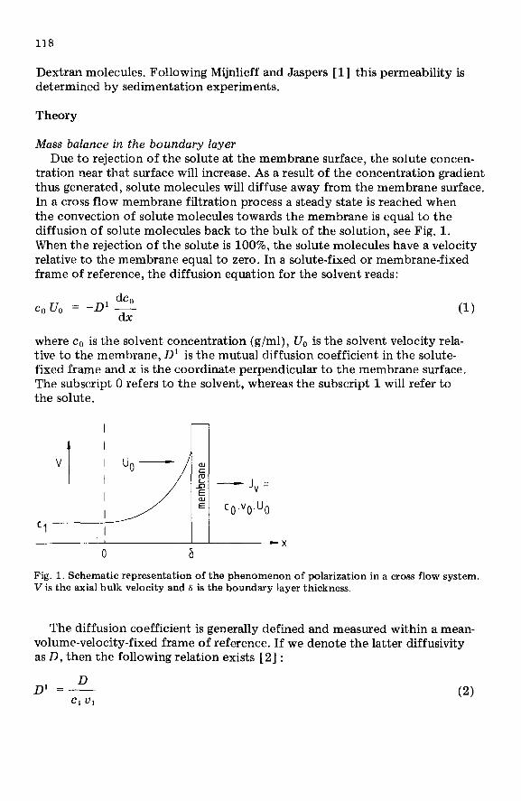
tration near that surface will increase. As a result of the concentration gradient thus generated, solute molecules will diffuse away from the membrane surface. In a cross flow membrane filtration process a steady state is reached when the convection of solute molecules towards the membrane is equal to the diffusion of solute molecules back to the bulk of the solution, see Fig. 1. When the rejection of the solute is lOO%, the solute molecules have a velocity relative to the membrane equal to zero. In a solute-fixed or membrane-fixed frame of reference, the diffusion equation for the solvent reads:

where co is the solvent concentration (g/ml), U. is the solvent velocity rela- tive to the membrane, D’ is the mutual diffusion coefficient in the solute- fixed frame and x is the coordinate perpendicular to the membrane surface. The subscript 0 refers to the solvent, whereas the subscript 1 will refer to the solute.

Fig. 1. Schematic representation of the phenomenon of polarization in a cross flow system. V is the axial bulk velocity and 6 is the boundary layer thickness.

The diffusion coefficient is generally defined and measured within a mean- volume-velocity-fixed frame of reference. If we denote the latter diffusivity as D, then the following relation exists [ 21 :

119

Since co u. + cl ul = 1, where u is the specific volume (ml/g) we have:

dco = - “1 dc, UO

and since the permeate volume flow J, = co u. U. , we can rewrite eqn. (1) as:

ClJ” = DdZ (4)

Equation (4) is the well known concentration polarization equation and the derivation given above clearly shows that the diffusion coefficient to be used in this equation is the volume-fixed coefficient, D.

Application of the film model for the mass transfer near the membrane surface gives the boundary conditions for eqn. (4):

x=0; cl=cb

x=6; c1=c, (5)

The boundary layer thickness, 6, is the quotient of D and the mass transfer coefficient k. The value of the diffusion coefficient depends on concentration; hence, it will vary over the boundary layer thickness and an averaged value for D must be used. Integration of eqn. (4) under the condition that J, is constant (steady state) yields:

c, = cb exP (Jvlk ) (6)

Force balance in the boundary layer Up to here, we have evaluated the mass balance of the boundary layer. In

the stationary boundary layer there is also a force balance: the net force acting’on each particle is zero. The solute molecules in the boundary layer are subject to a thermodynamic force directed to the bulk of the solution due to the gradient in their chemical potential. The force balance implies that the drag force exerted by the solvent flow on the solute molecules per gram of solute, F, , is equal to

&I dv: dP F1 =- =-+lJ1---

dx dx dx (7)

where p is the chemical potential per gram, pc is the concentration part of the chemical potential and P is the hydraulic pressure. In eqn. (7) it is assumed that only concentration and pressure gradients are present in the boundary layer. The balance of the drag forces yields for the drag force exerted by the solute molecules on the solvent flow per gram solvent, Fo:

coFo +c,F1 = 0 (8)

120

This drag force, FO, is balanced in turn by the force due to the chemical potential gradient of the solvent, so:

dpo d/-6 dP FO =- =----tQ--

dx dx dx (9)

The Gibbs-Duhem relation reads:

cOdp:+c,d/J = 0 (10)

and inserting eqns. (7) and (9) into eqn. (8) and applying eqn. (10) we obtain:

dP dP COUO - + Cl Ul - = 0

dx dx

From eqn. (11) it is clear that

dP -= 0 dx

(11)

(12)

which means that in the boundary layer there is no pressure drop. The solvent flow is subject to a hydrodynamic boundary layer resistance but the energy dissipation in this layer is exactly compensated by the decrease in the chemical potential of the solvent due to its concentration gradient. Equations (8) and (12) are valid only if the complete boundary layer has the properties of a Newtonian fluid. Viscoelastic behaviour in the boundary layer or forma- tion of a gel layer will give rize to a pressure drop outside the membrane.

Dejmek [3] was the first to analyze the force balance in a concentration polarization layer, but he did not reach the conclusion that the pressure drop in the boundary layer was zero. Wales [4] showed clearly that dP/dx = 0, using an approach somewhat different from that used by us. Wales restricted his analysis to laminar boundary layers. In his opinion there is no assurance that dP/dx = 0 in turbulent boundary layers where, as well as molecular diffusion, eddy diffusion is also operative. Contrary to this view, we think that in turbulent flow systems also the pressure drop in the boundary layer is zero. We have two arguments for this: (i) in the analysis given above no diffusion coefficient was used, and (ii) in the film theory for mass transfer the boundary layer is evaluated as a stagnant layer with a thickness 6, which is determined by both the molecular and eddy diffusivity.

Hydrodynamic resistance of the boundary layer The boundary layer in ultrafiltration can be seen as a stagnant, concentrated

polymer solution through which the solvent permeates. For polymer concen- trations exceeding the “overlap” concentration, where the individual domains of the polymer molecules touch each other, the solvent molecules have to flow through the polymer coils. In more dilute solutions the solvent flow takes place mainly around the polymer coils. According to Mijnlieff and

121

Jaspers [l] the permeability of such a stagnant polymer solution can be calcu- lated from a totally different experimental situation: sedimentation in an analytical ultracentrifuge cell. This follows from their analysis of the flow equations for sedimentation and permeation; they have obtained:

770s

P= Cl(l - Wo)

(13)

where s is the sedimentation coefficient of the polymeric solute and q. is the dynamic viscosity of the solvent. The permeability, p, has been defined by Darcy [5] and remembering that in the boundary layer the osmotic pressure gradient is the driving force for the solvent flow, see Fig. 2, we have:

c p dII J, =--y- (14)

vo dx . ,

Integration of eqn. (14) over the thickness of the boundary layer yields:

J, = Anbl

~oS:p-Qx (15)

where AIlbl is the osmotic pressure difference over the boundary layer. The permeability depends on the concentration and since there is a concentration profile in the boundary layer, the permeability will be a function of the coordinate x. Thus, the hydrodynamic resistance of the boundary layer, Rbl, is defined as:

&,I = j p(x)-’ dx 0

(16)

I r-l n

0 a) 6 0 b) 8

Fig. 2. Gradients of pressure (a) and chemical potential (b) in and near the membrane in an ultrafiltration process.

Expression for the permeate flux In the preceeding sections we have shown that, although the boundary layer

is responsible for a hydrodynamic resistance, there is no drop in hydraulic

122

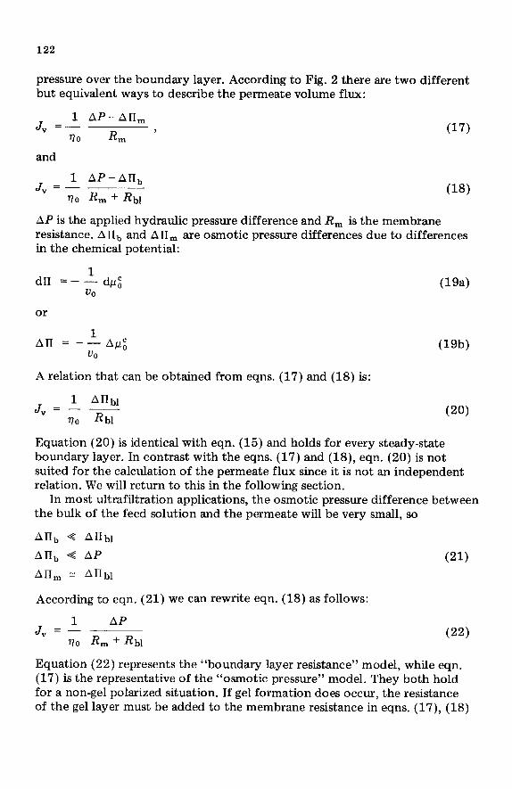
pressure over the boundary layer. According to Fig. 2 there are two different but equivalent ways to describe the permeate volume flux:

1 AP-An, J, =-

170 R, ’ (17)

and

1 AP-AIlI, J, = -

170 Rm + Rt,l

AP is the applied hydraulic pressure difference and R, is the membrane resistance. A Ilb and All, are osmotic pressure differences due to differences in the chemical potential:

dn = - t d& UO

(Iga)

or

Ail = -LA& vo

A relation that can be obtained from eqns. (17) and (18) is:

J, = _f anbl BO Rbl

Wb)

WV

Equation (20) is identical with eqn. (15) and holds for every steady-state boundary layer. In contrast with the eqns. (17) and (US), eqn. (20) is not suited for the calculation of the permeate flux since it is not an independent relation. We will return to this in the following section.

In most ultrafiltration applications, the osmotic pressure difference between the bulk of the feed solution and the permeate will be very small, so

AII, < Anbl

AII,, < AP

AII, = AIIbl

According to eqn. (21) we can rewrite eqn. (18) as follows:

J, = _!_ AP

vo Rm + Rbl

(21)

(22)

Equation (22) represents the “boundary layer resistance” model, while eqn. (17) is the representative of the “osmotic pressure” model. They both hold for a non-gel polarized situation. If gel formation does occur, the resistance of the gel layer must be added to the membrane resistance in eqns. (17), (18)

123

and (22). It is emphasized here that if one uses the osmotic pressure model, one implicitly assumes that dP/dx = 0 in the boundary layer.

Relationship between permeation, diffusion and osmotic pressure Comparing eqn. (4) with eqn. (14) we see that there must exist a relation-

ship between diffusivity, permeability and the dependency of the osmotic pressure on concentration. The relation between sedimentation and diffusion is given by the Svedberg equation [6] :

(23)

Here, p is the density of the solution (p = c0 + cl). With the help of eqns. (10) and (19) and using

(l- &P) = uoc*(I - UI/UO)

we obtain

(24)

s dlI

D = (1 - ul/uo) dc,

Substitution of eqn. (13) into eqn. (25) yields:

CIP dn D =--

vo dc, (26)

This relation between diffusivity and permeability makes eqns. (4) and (14) equivalent. Mijnlieff and Jaspers [l] previously pointed out that there is one basic phenomenological relation which describes permeation, sedimentation and diffusion, and eqn. (26) is the result of this connection.

The interdependency of permeability and diffusion coefficient has also been investigated by McDonnell and Jamieson [7]. The expression obtained by them differs from our eqn. (26) by a factor puo, which originates from the fact that they have used the diffusion equation of the mass-fixed reference frame instead of the volume-fixed reference frame.

Experimental

Ultrafiltration The ultrafiltration experiments were carried out in a thin channel cell using

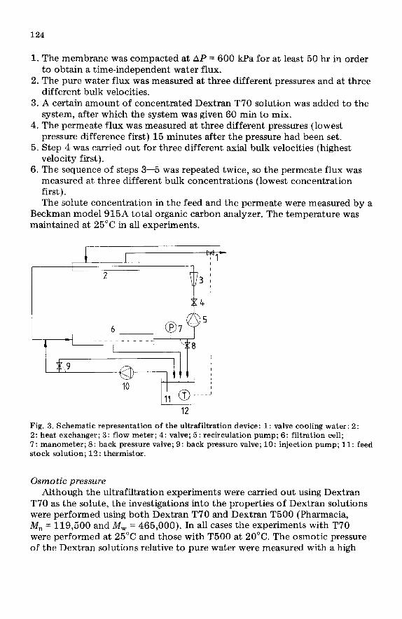
solutions of Dextran T70 (Pharmacia, M, = 36,200 and M, = 70,300) in water (ultrafiltrated, demineralized) as the feed. The cell had an effective membrane width of 60 mm and a channel height of 5.9 mm. The membrane area length was 100 mm and the length of the entrance region was 250 mm. The mem- branes used were Kalle polysulfone membranes of the Nadir type. The experi- mental set-up is shown in Fig. 3; the experimental procedure was as follows:

124

1. The membrane was compacted at AP = 600 kPa for at least 50 hr in order to obtain a time-independent water flux.

2. The pure water flux was measured at three different pressures and at three different bulk velocities.

3. A certain amount of concentrated Dextran T70 solution was added to the system, after which the system was given 60 min to mix.

4. The permeate flux was measured at three different pressures (lowest pressure difference first) 15 minutes after the pressure had been set.

5. Step 4 was carried out for three different axial bulk velocities (highest velocity first).

6. The sequence of steps 3-5 was repeated twice, so the permeate flux was measured at three different bulk concentrations (lowest concentration first). The solute concentration in the feed and the permeate were measured by a

Beckman model 915A total organic carbon analyzer. The temperature was maintained at 25°C in all experiments.

Fig. 3. Schematic representation of the ultrafiltration device: 1: valve cooling water; 2 : 2: heat exchanger; 3: flow meter; 4: valve; 5: recirculation pump; 6: filtration cell; ‘7 : manometer; 8 : back pressure valve; 9 : back pressure valve; 10: injection pump; 11: feed stock solution: 12 : thermistor.

Osmotic pressure Although the ultrafiltration experiments were carried out using Dextran

T70 as the solute, the investigations into the properties of Dextran solutions were performed using both Dextran T70 and Dextran T500 (Pharmacia, M, = 119,500 and M, = 465,000). In all cases the experiments with T70 were performed at 25°C and those with T500 at 20°C. The osmotic pressure of the Dextran solutions relative to pure water were measured with a high

125

pressure osmometer [8]. The membranes used in the osmometer were Sartorius “allerfeinst”.

Sedimentation coefficient Sedimentation experiments were performed with a Beckman-Spinco

Model E analytical ultracentrifuge. The sedimentation coefficients were deter- mined at different concentrations from the displacement of the maximum of the concentration gradient curve.

In order to calculate the permeability from the sedimentation coefficient, the specific volume of the Dextrans in water had to be known. This quantity was calculated from the slope of the solution density versus concentration plot. Densities were measured with a Paar digital precision density meter, model DMA 50.

Diffusion coefficient The diffusion coefficients were determined by the boundary layer broadening

method using a synthetic boundary cell of the ultracentrifuge mentioned above. The concentration difference at the boundary at the beginning of each experi- ment was at the most 0.026 g/ml and smaller than 0.01 g/ml in most cases. The concentrations mentioned further on are the mean concentrations. The diffusion coefficients obtained with this kind of experiment are the volume- fixed diffusion coefficients.

Results and discussion

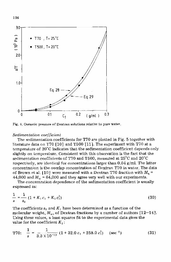
Osmotic pressure The osmotic pressure data for both Dextran T70 and T500 are given in

Fig. 4. The osmotic pressure in a broad concentration range is conveniently represented by the general form [9] :

AlI = AleI +A& +A&

A least squares fit to the experimental data of Fig. 4 gives:

(27)

T70: Ail = 0.375 cl + 7.52 c: + 76.4 c: (10’ Pa) (28)

T500: Ail = 0.0867 c1 + 2.98 c: + 89.8 CT (lo5 Pa) (29)

According to van ‘t Hoff’s law, the coefficient Al of eqn. (27) must be equal to R T/M,. The values of R T/1&&., are 0.684 and 0.204 X 10’ Pa-ml/g for T70 and T500, respectively, so there is a substantial deviation. The origin for this deviation is probably that the osmotic experiments were carried out with concentrations larger than 0.05 g/ml. Equation (27) reduces to the van ‘t Hoff law in very dilute solutions only. Since we are interested in the osmotic pressure of more concentrated solutions, eqns. (28) and (29) are used to express the concentration dependence of A Il. From Fig. 4 it is clear that the influence of M, on the osmotic pressure is relatively small for concen- trated solutions.

126

0.1 Cl o.2 ( g/ml 1

Fig. 4. Osmotic pressure of Dextran solutions relative to pure water.

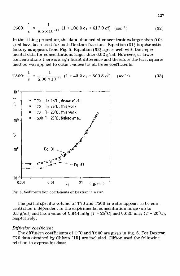
Sedimentation coefficient The sedimentation coefficients for T70 are plotted in Fig. 5 together with

literature data on T70 [IO] and T500 [ll]. The experiment with T70 at a temperature of 20°C indicates that the sedimentation coefficient depends only slightly on temperature. Consistent with this observation is the fact that the sedimentation coefficients of T70 and T500, measured at 25°C and 20°C respectively, are identical for concentrations larger than 0.04 g/ml. The latter concentration is the overlap concentration of Dextran T70 in water. The data of Brown et al. [lo] were measured with a Dextran T70 fraction with M, = 44,000 and M, = 64,000 and they agree very well with our experiments.

The concentration dependence of the sedimentation coefficient is usually expressed as:

1 -=$(1+&c, + K2 c:, (30) S

The coefficients s0 and K1 have been determined as a function of the molecular weight, M,, of Dextran fractions by a number of authors [12-141. Using these values, a least squares fit to the experimental data gives the value for the coefficient K, :

1 1 T70: - =

3.3 x lo-l3 (1 + 32.0 cl + 258.0 c:) (set-‘)

s (31)

127

T500: t = 1

- (1 + 106.0 cl + 617.0 CT) (set-‘) S 8.5 X lo-l3

(32)

In the fitting procedure, the data obtained at concentrations larger than 0.04 g/ml have been used for both Dextran fractions. Equation (31) is quite satis- factory as appears from Fig. 5. Equation (32) agrees well with the experi- mental data for concentrations larger than 0.02 g/ml. However, at lower concentrations there is a significant difference and therefore the least squares method was applied to obtain values for all three coefficients:

T500: 1 = 1

5.06 X lo-l3 (1 + 43.2 cl + 500.8 cf) (see-‘)

s

1o15 ,

7 IA

lOI -

T IA

lOI -

0 T70 ,T= 25’C, Brown etal. n T70 ,T= 25’C, this work

. T70 ,T= ZO’C, this work

l TSOO,T= 20'C,Nakaoetal.

Eq. 31

0.01 Cl

0.1 ( g/ml 1 ’

Fig. 5. Sedimentation coefficients of Dextran in water.

The partial specific volume of T70 and T500 in water appears to be con- centration independent in the experimental concentration range (up to 0.3 g/ml) and has a value of 0.644 ml/g (T = 25°C) and 0.625 ml/g (7’ = 20”(Z), respectively.

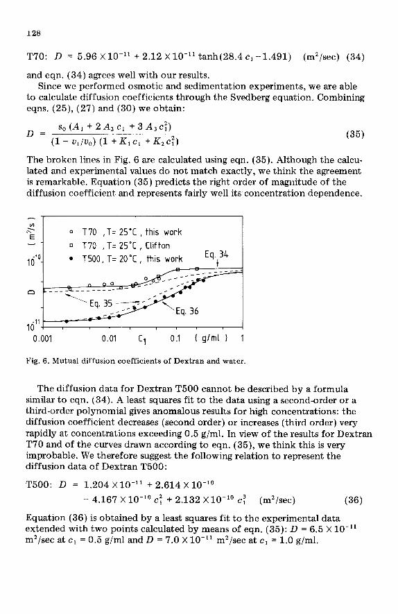
Diffusion coefficient The diffusion coefficients of T70 and T500 are given in Fig. 6. For Dextran

T70 data obtained by Clifton [15] are included. Clifton used the following relation to express his data:

128

T70: D = 5.96 X lo-” + 2.12 X1O-1’ tanh(28.4 c1 -1.491) (m’/sec) (34)

and eqn. (34) agrees well with our results. Since we performed osmotic and sedimentation experiments, we are able

to calculate diffusion coefficients through the Svedberg equation. Combining eqns. (25), (27) and (30) we obtain:

D= sO(Al +2A,c, +3A&)

(1 - wA3) (1 + K1 Cl + &CT) (35)

The broken lines in Fig. 6 are calculated using eqn. (35). Although the calcu- lated and experimental values do not match exactly, we think the agreement is remarkable. Equation (35) predicts the right order of magnitude of the diffusion coefficient and represents fairly well its concentration dependence.

I I

3 E

0 T70 ,T= 25°C , this work

q T70 ,T= 25'C, Clifton

do- * TSOO, T= 2O'C, this work

OL

ld"l 0.001 0.01 c, 0.1 ( g/ml I 1

Fig. 6. Mutual diffusion coefficients of Dextran and water.

The diffusion data for Dextran T500 cannot be described by a formula similar to eqn. (34). A least squares fit to the data using a second-order or a third-order polynomial gives anomalous results for high concentrations: the diffusion coefficient decreases (second order) or increases (third order) very rapidly at concentrations exceeding 0.5 g/ml. In view of the results for Dextran T70 and of the curves drawn according to eqn. (35), we think this is very improbable. We therefore suggest the following relation to represent the diffusion data of Dextran T500:

T500: D = 1.204 X1O-1’ + 2.614 X lo-”

- 4.167 X lo-” c: + 2.132 X lo-” c: (m”/sec) (36)

Equation (36) is obtained by a least squares fit to the experimental data extended with two points calculated by means of eqn. (35): D = 6.5 X lo-” m2/sec at cl = 0.5 g/ml and D = 7.0 X 10-l’ m2/sec at c, = 1.0 g/ml.

129

Ultrafiltration The permeate flux versus applied pressure data obtained with the ultra-

filtration experiments are represented in Fig. 7. The permeate flux increases with increasing pressure, although the slope of the J, versus AP plot decreases with increasing AP. The slope does not become zero (“limiting flux”) under the circumstances studied. Furthermore, the permeate flux decreases with an increasing bulk concentration and with a decreasing axial bulk velocity. All this is in full accordance with the osmotic pressure model for ultrafiltration [ 161. The rejection of the T70 molecules by the membrane decreased with increasing pressure, with an increasing bulk concentration and with a decreasing axial velocity. The lowest rejection value was 96% and the rejection was higher than 98% in all but three experiments.

Pure water flux increased linearly with AP and thus the membrane resis- tance was independent of the applied pressure and did not vary with the axial velocity. This indicates that fouling of the membrane by the ultrafiltrated water did not occur and that R, has a constant value of 6.94 X 1Ol2 m-‘.

10 , / I / I /

0 AP 600 0 AP 600 0 AP (kPa) 600

Fig. 7. Ultrafiltration permeate fluxes as a function of applied pressure, axial bulk velocity and bulk concentration. The bulk concentrations are 0.000430, 0.000935 and 0.00142 g/ml; -: pure water flux.

Resistance of the boundary layer The resistance of the boundary layer can be computed from Fig. 7 using

eqn. (22). This experimental value for &-,I, denoted REP, will be compared with the value calculated from eqn. (16) using the sedimentation and diffu- sion data. The expression for this R$ is derived as follows.

According to eqn. (13) and (30) we express the permeability of the dis- solved Dextran molecules as:

voso IJCcl) = (1 - ul/vo) (Cl + K1 c: + K2 c:>

(37)

130

The concentration of the solute in the boundary layer is a function of the co- ordinate x and since the rejection is almost 100% we write, see eqn. (6):

Substitution of eqn. (38) into eqn. (37) yields:

(33)

p(x)-’ = 1 - h/U0

bb exp tJv x/D) rloso

+ K1 cl: exp (2 J,x/D) + Kz c1: exp (3J, x/D)] (39)

The quantity p (x)-l must be integrated over the boundary layer thickness, 6, and since

6

Ckt s exp (nJ”x/D)dx = % c: [exp (G/k) - 11 0 v

D (ck - c;> =-

Jvn

we obtain

6 pale =

bl s p(x)-’ dx 0

D l-q/u, Kl =- JV

cm - cb + - (c; - c;) + 77oso 2

(40)

(41)

Combining eqns. (41), (6) and (22) we obtain a relationship in which the permeate flux, J,, is the single unknown parameter. In this way, J, can be calculated if the process conditions (AP, R,, cb and h) and the physical properties of the solute-solvent system (s and D) are known.

Values for the mass transfer coefficient, .lz, are obtained in the following way. With the help of eqn. (17) the osmotic pressure difference over the membrane is calculated from the permeate flux data. The results are given in Table 1. From AlI, and the osmotic pressure data, the value of c, is com- puted. The maximum value for c, appears to be 0.364 g/ml (Table 1) and since Dextran T70-water mixtures with concentrations up to 0.7 g/ml are fluid, we conclude that in all experiments reported here no gel layer has been formed,

Using eqn. (6) and the c, values given in Table 1, the apparent mass trans- fer coefficient kapp can be calculated. In Fig. 8 this kaPP is compared with the mass transfer coefficient, k, as obtained from the Deissler equation for turbulent systems:

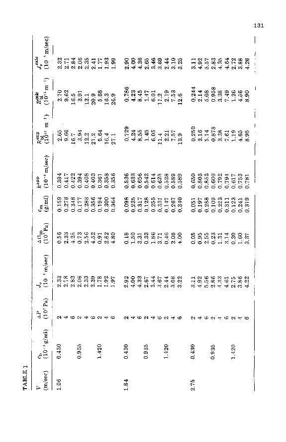
TABLE1

J”

(10m5 m/set)

AII,

C

lll

,,+P

R

CaJ

C

bl

(lOsPa)

(g/ml) (10m5m/sec)

m-l)

(lO1'm-')

1.06

0.430

2

2.33

0.56

0.159

0.39

4 2.65

2.70

2.32

4

2.78

2.33

0.278 0.417

9.66

9.62

,2.71

6

2.83

4.25

0.348 0.422

16.7

16.5

2.84

0.935

2

2.06

0.73

0.177 0.394

3.94

3.91

2.06

4

2.33

2.56

0.288 0.408

12.2

12.1

2.35

6

2.39

4.52

0.356 0.403

21.2

20.9

2.41

1.420

2

1.78

0.91

0.194 0.361

5.64

5.68

1.77

4

1.92

2.82

0.300 0.358

16.4

16.3

1.93

6

1.97

4.80

0.364 0.356

27.1

26.9

1.99

34

0.430

2

2.92

0.18

0.098

0.536

0.72

9 0.786

2.90

4

4.00

1.50

0.235 0.633

4.24

4.23

4.00

6

4.33

3.31

0.317 0.656

8.55

8.45

4.36

0.935

2

2.67

0.33

0.128 0.542

1.45

1.47

2.65

4

3.44

1.86

0.255 0.614

6.05

6.01

3.46

6

3.67

3.71

0.331 0.625

11.4

11.2

3.69

1.420

2

2.44

0.46

0.147 0.528

2.21

2.19

2.44

4

3.08

2.08

0.267 0.589

7.57

7.53

3.10

6

3.22

4.00

0.340 0.589

13.9

12.6

3.25

2.75

0.430

2

3.11

0.05

0.051 0.650

0.250

0.244

3.11

4

4.92

0.95

0.197 0.803

2.16

2.14

4.92

6

5.56

2.55

0.288 0.853

5.14

5.08

5.57

0.935

2

2.86

0.23

0.109 0.600

0.878

0.958

2.83

4

4.33

1.31

0.223 0.792

3.38

3.38

4.35

6

4.61

3.14

0.311 0.794

7.61

7.49

4.64

1.420

2

2.75

0.30

0.123 0.617

1.19

1.26

2.72

4

3.86

1.60

0.241 0.753

4.65

4.56

3.88

6

4.22

3.37

0.319 0.781

8.95

8.90

4.26

-.

JF

(10-5m/sec)

(42)

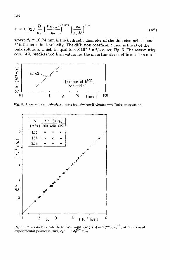
where dh = 10.74 mm is the hydraulic diameter of the thin channel cell and V is the axial bulk velocity. The diffusion coefficient used is the D of the bulk solution, which is equal to 4 X lo-l1 m2/sec, see Fig. 6. The reason why eqn. (42) predicts too high values for the mass transfer coefficient is in our

1 V 10 ( m/s 1 loo

Fig. 8. Apparent and calculated mass transfer coefficients; -: Deissler equation.

./ /

i 7 .

6’ 0’

9’ do

9’

4 ( 10e5 m/s I 6

Fig. 9. Permeate flux calculated from eqns. (41), (6) and (22), JrlC, as function of experimental permeate flux, Jv; -: JvcalC = Jv.

133

opinion that no account has been made for the increase in viscosity in the boundary layer, nor for the effect of the permeate flux on the boundary layer.

The haPP values are used to calculate the permeate flux and the result, Jzdc, is displayed in the last column of Table 1. The averaged value of 6 X lo-l1 m2/sec has been used in this calculation. In Fig. 9 the value of &? is plotted as a function of J,. The value of J, is calculated using eqn. (22), thus neglecting the osmotic pressure of the bulk solution. The osmotic pres- sure data show that this approach is valid. As can be seen from Fig. 9, the correlation between Jzalc and J, is excellent. In the calculation procedure the values for the boundary layer resistance Rgp are also obtained and these values are compared in Table 1 with R Kp .The correlation is very good for R,, values varying by more than two orders of magnitude, which in view of the close agreement of J, and JGalc was expected. These results imply that the approach of calculating the resistance of the boundary layer with aid of the permeability of the Dextran molecules works well, as was already pre- dicted in the theory section. In general, one can say that the stationary boundary layer in ultrafiltration can be seen as a diffusion-permeation equilibrium.

Conclusions

The permeate flux in ultrafiltration applications is smaller than the pure solvent flux due to the formation of a concentration polarization boundary layer. The effect of this concentrated but still fluid boundary layer can be represented in two different ways: (i) by a reduction of the driving force by a an osmotic pressure (the osmotic pressure model), and (ii) by an increase of the total resistance due to the resistance of the boundary layer (the resistance model). It is shown that these two approaches are essentially equivalent and that the resistance of the boundary layer can be computed with the solvent permeability of the macromolecular solute.

List of symbols

Ai CO Cl

cb cm dh D D'

Fo F* J”

coefficient in eqn. (27), i = 1,2,3 (Pa-mli/gi) solvent concentration (g/ml) solute concentration (g/ml) solute concentration in bulk (g/ml) solute concentration at membrane surface (g/ml) hydraulic diameter (m) diffusion coefficient in volume-fixed frame (m*/sec) diffusion coefficient in solute-fixed frame (m”/sec) drag force on solvent (N/g) drag force on solute (N/g) permeate volume flux (m/set)

134

JF k

Ki

so T

ucl UO

Ul

V X

J, from eqns. (6), (22) and (41) (mjsec) mass transfer coefficient (m/set) coefficient in eqn. (30), i = 1,2 (ml’/g’) number-averaged molecular weight (dalton) weight-averaged molecular weight (dalton) solvent permeability of the solute (m’) gas constant (J/mol-K) resistance of boundary layer (m-l) Rb, from eqns. (6), (22) and (41) (m-l) Rbl from eqn. (22) and flux data (m-l) resistance of membrane (m-l) sedimentation coefficient of the solute (set) s at infinite dilution (set) temperature (K) or (“C) velocity of solvent relative to the membrane (m/set) partial specific volume of the solvent (ml/g) partial specific volume of the solute (ml/g) axial bulk velocity (m/set) coordinate perpendicular to the membrane surface (m)

thickness of boundary layer (m) hydraulic pressure difference (Pa) osmotic pressure difference (Pa) AII of bulk solution relative to permeate (Pa) An over boundary layer (Pa) AR over membrane (Pa) chemical potential of the solvent (N/m-g) concentration part of ,uo (N/m-g) chemical potential of the solute (N/m-g) concentration part of I-(~ (N/m-g) viscosity of the solvent (Pa-see) solution density (g/ml) density of the solvent (g/ml)

References

1 P.F. Mijnlieff and W.J.M. Jaspers, Solvent permeability of dissolved polymer material. Its direct determination from sedimentation experiments, Trans. Faraday Sot., 67 (1971) 6 1837.

2 S.R. de Groot and P. Mazur, Non-equilibrium Thermodynamics, North-Holland Publishing Company, Amsterdam, 1962, p. 251.

3 P. Dejmek, Concentration polarization in ultrafiltration of macromolecules, Ph.D. Thesis, Lund Institute of Technology, Lund, 1975.

4 M. Wales, Pressure drop across polarization layers in ultrafiltration, Amer. Chem. Sot., Symp. Ser., 154 (1981) 159.

5 H. Darcy, Les fontaines publiques de la ville de Dijon, 1856. 6 T. Svedberg and K.O. Pedersen, The Ultracentrifuge, Clarendon Press, Oxford, 1940.

135

8 9

10

11

12

13

14

15

16

M.E. McDonnell and A.M. Jamieson, Application of the porous-sphere hydrodynamic model to dilute polymer solutions, J. Polym. Sci., Polym. Phys. Ed., 18 (1980) 1781. F.W. Altena, Ph.D. Thesis, Twente University of Technology, Enschede, 1982. P.J. Flory, Principles of Polymer Chemistry, Cornell University Press, Ithaca, 1953, p. 531. W. Brown, P. Stilbs and R.M. Johnsen, Self-diffusion and sedimentation of Dextran in concentrated solutions, J. Polym. Sci., Polym. Phys. Ed., 20 (1982) 1771. S. Nakao, J.G. Wijmans and C.A. Smolders, Resistance to the permeate flux in unstirred ultrafiltration. Part II. Dissolved macromolecular solutions, to be submitted to J. Membrane Sci. F.R. Senti, N.N. Hellman, N.H. Ludwig, G.E. Babbcock, R. Tobin, C.A. Glass and B.L. Lamberts, Viscosity, sedimentation and light scattering properties of fractions of an acid-hydrolyzed Dextran, J. Polym. Sci., 17 (1955) 527. A.G. Ogston and E.F. Woods, The sedimentation of some fractions of degraded Dextran, Trans. Faraday Sot., 50 (1954) 635.

J.W. Williams and W.M. Saunders, Size distribution analysis in plasma extender systems. II. Dextran, J. Phys. Chem., 58 (1954) 854. M.J. Clifton, Polarisation de concentration dans divers pro&d&s de separation a membrane, Ph.D. Thesis, Universite Paul Sabatier, Toulouse, France, 1982. J.G. Wijmans, S. Nakao and C.A. Smolders, Flux limitation in ultrafiltration: Osmotic pressure model and gel layer model, J. Membrane Sci., 20 (1984) 115.