arX

iv:0

910.

3994

v1 [

mat

h.PR

] 2

1 O

ct 2

009

Hydrodynamic limit for two-species exclusion processes

Makiko Sasada

Graduate School of Mathematical Sciences,

The University of Tokyo, Komaba, Tokyo 153-8914, Japan

e-mail: sasada@ms.u-tokyo.ac.jp

Abstract

We consider two-species exclusion processes on the d-dimensional discrete torus takingthe effects of exchange, creation and annihilation into account. The model is, ingeneral, of nongradient type. We prove that the (charged) particle density convergesto the solution of a certain nonlinear diffusion equation under the diffusive rescalingin space and time. We also prove a lower bound on the spectral gap for the generatorof the process confined in a finite volume.

Keywords: hydrodynamic limit; interacting particle systems; two-species exclusion pro-cesses

1 Introduction

The aim of this paper is to obtain the hydrodynamic behavior of two-species exclusionprocesses. Our results can be applied to establish the hydrodynamic limit for the evolutionof height differences in interfaces governed by the 1-dimensional SOS dynamics.

The two-species exclusion process describes the evolution of a system of mechanicallydistinguishable particles, say +particles and −particles moving on a discrete lattice spaceunder the constraint that at most one particle can occupy each site. The state space ofthe process is given by −1, 0, 1TdN where TdN stands for the d-dimensional discrete toruswith side-length N and its elements (called configurations) are denoted by η = (η(x), x ∈TdN ), with η(x) = 0 or 1 or −1 depending on whether x ∈ TdN is empty or occupiedby a +particle or a −particle, respectively. Each ± particle moves to a neighboringempty site with the constant jump rate C± > 0, respectively. Two different types ofneighboring particles exchange their locations with the constant rate CE ≥ 0. Also theyannihilate simultaneously when they are neighboring with the constant rate CA ≥ 0, andtwo different types of particles are created with the constant rate CC ≥ 0 if two emptysites are neighboring.

In this paper, we consider the case where CA > 0 or CC > 0, so that the process has aunique conserved quantity

∑

x∈TNdη(x). We prove the hydrodynamic limit for the profile

associated with this quantity and obtain the explicit expression of the diffusion coefficient.

Tel.: +81-3-5465-7001; Fax: +81-3-5465-7011 (M.Sasada).MSC: primary 60K35, secondary 82C22.

1

We classify the dynamics into three types as the case where CA > 0 and CC > 0 (Case1), CA > 0 and CC = 0 (Case 2) and CA = 0 and CC > 0 (Case 3) and give proofsseparately. For Cases 2 and 3, we assume the gradient condition so far. We can show thatall of the hydrodynamic equations of our processes have a diagonal diffusion coefficientmatrix, therefore they have unique weak solutions without the smoothness of the diffusioncoefficient.

Quastel proved the hydrodynamic limit for two-colored simple exclusion process in [6].This process is corresponding to the model with C+ = C− > 0 and CA = CC = CE = 0,so it is not included in our cases.

The SOS dynamics describe the evolution of the integer-valued heights of interfaceson the discrete lattice. In the 1-dimensional case, the height difference of SOS dynamicsand the configuration of the two-species exclusion process have one-to-one correspondence,see, e.g. [1].

This paper is organized as follows: In Section 2 we introduce our model and state themain results for three types of models respectively. In Section 3, we give the proof of themain theorem for Case 1. In the proof, we give a spectral gap estimate and characterizethe class of closed forms. In Sections 4 and 5, we give the proofs of the main theoremsfor Cases 2 and 3, respectively. In Section 6, we state the uniqueness results for nonlinearparabolic equations whose diffusion coefficient matrices are diagonal.

2 Model and Main Results

The two-species exclusion process is a Markov process ηt on the configuration space χdN =

−1, 0, 1TdN , where TdN = (Z/NZ)d is the d-dimensional discrete torus. The dynamics aredefined by means of an infinitesimal generator LN acting on functions f : χdN → R as

(LNf)(η) =∑

b∈(TdN)∗

Lbf(η),

where (TdN )∗ stands for the set of all directed bonds b = (x, y), i.e., the ordered pairs of

x, y ∈ TdN such that |x − y| = 1 where |x − y| = ∑

1≤i≤d |xi − yi| is the sum norm in Rd.

Here, for each bond b ∈ (TdN )∗,

(2.1) Lbf(η) = cb(η)(πbf)(η),

where

(πbf)(η) = [1η(x)=1,η(y)=0 + 1η(x)=0,η(y)=−1 + 1η(x)=−1,η(y)=1 ](f(ηx,y)− f(η))

+ 1η(x)=1,η(y)=−1(f(ηx=0,y=0)− f(η)) + 1η(x)=0,η(y)=0(f(η

x=−1,y=1)− f(η)),

and

cb(η) = C+1η(x)=1,η(y)=0 + C−1η(x)=0,η(y)=−1 + CE1η(x)=−1,η(y)=1

+ CA1η(x)=1,η(y)=−1 + CC1η(x)=0,η(y)=0 .

2

In the above formula, ηx,y, ηx=−1,y=1 and ηx=0,y=0 ∈ χdN stand for

ηx,y(z) =

η(z) if z 6= x, y,

η(y) if z = x,

η(x) if z = y,

ηx=−1,y=1(z) =

η(z) if z 6= x, y,

−1 if z = x,

1 if z = y,

and

ηx=0,y=0(z) =

η(z) if z 6= x, y,

0 if z = x,

0 if z = y,

respectively, and we assume that C+ and C− are positive constants and CA, CC and CEare nonnegative constants.

We will use the following simplified notations

η(x,y) =

ηx,y if (η(x), η(y)) = (1, 0) or (0,−1) or (−1, 1),

ηx=0,y=0 if (η(x), η(y)) = (1,−1),

ηx=−1,y=1 if (η(x), η(y)) = (0, 0),

Ψx,ya,b (η) = 1η(x)=a,η(y)=b ,

and define rb for b ∈ (TdN )∗ by

rb(η) = Ψx,y1,0(η) + Ψx,y

0,−1(η) + Ψx,y−1,1(η) + Ψx,y

1,−1(η) + Ψx,y0,0(η).

With these notations, Lb and πb can be rewritten as

Lbf(η) = cb(η)(f(η(x,y))− f(η)),

πbf(η) = rb(η)(f(η(x,y))− f(η)),

respectively.

The process is reversible with respect to the following one parameter family of trans-lation invariant product measures νρ.

Definition 2.1. For each fixed ρ ∈ [−1, 1], let νρ be a product measure on χdN withmarginals given by

νρη(x) = 1 =1− Φ(ρ) + ρ

2,

νρη(x) = 0 = Φ(ρ),

νρη(x) = −1 =1− Φ(ρ)− ρ

2,

3

for all x ∈ TdN , where

Φ(ρ) =

1−√

4β+ρ2−4βρ2

1−4β if β 6= 14

1−ρ2

2 if β = 14

with β = CC/CA. Especially, if CA > 0, CC = 0, then

νρη(x) = 1 = ρ ∨ 0,

νρη(x) = 0 = 1− |ρ|,νρη(x) = −1 = |ρ ∧ 0|,

and if CA = 0, CC > 0, then

νρηx = 1 =1 + ρ

2,

νρηx = 0 = 0,

νρηx = −1 =1− ρ

2.

The index ρ stands for the density of particles with charge, namely Eνρ [η(0)] = ρ. Wewill abuse the same notation νρ for the product measures on the configuration spaces χdNor χd = −1, 0, 1Zd on the torus or on the infinite lattice. The expectation with respectto νρ will be sometimes denoted by

∫

f(η)νρ(dη) = 〈f〉ρ.

From the definition, our model satisfies the detailed balance condition, namely, forany directed bond b = (x, y),

(2.2) cb(η)νρ(η) = cb′(η(x,y))νρ(η

(x,y))

holds, where b′ = (y, x) is the reversed bond of b.

Here and after, we call f a cylinder function on χd if f depends on the configurationsonly through a finite set of coordinates. For any directed bond b = (x, y) and cylinderfunctions f , g, let us define Db(νρ; f, g) and Db(νρ; f) by

Db(νρ; f, g) := 〈−(Lb + Lb′)f, g〉ρ

andDb(νρ; f) := Db(νρ; f, f),

where b′ = (y, x) and 〈·, ·〉ρ stands for the inner product in L2(νρ). The reversibility (2.2)implies

(2.3) Db(νρ; f, g) = 〈cb(πbf)(πbg)〉ρ.

Let τx be the shift operator acting on the set A ⊂ Zd and cylinder functions f as wellas configurations η as follows:

4

τxA := x+A, τxf(η) = f(τxη), (τxη)(z) := η(z − x), z ∈ Zd.

For every cylinder function g : χd → R, consider the formal sum

Γg :=∑

x∈Zd

τxg

which does not make sense but for which the gradient

πΓg = (π0,e1Γg, ..., π0,edΓg)

is well defined.

We are now in a position to define the diffusion coefficient. For each ρ ∈ [−1, 1],define

d(ρ) =1

χ(ρ)infgD0,e(νρ; η(0) + Γg)

where infg is taken over all cylinder functions g and e is a unit vector of arbitrary direction.In this formula χ(ρ) stands for the so-called static compressibility which in our case is equalto

χ(ρ) = 〈η(0)2〉ρ − 〈η(0)〉2ρ = 1− Φ(ρ)− ρ2

Notice that d(ρ) does not depend on the choice of a unit vector ei, 1 ≤ i ≤ d.

For a probability measure µN on χdN , we denote by PµN the distribution on the path

space D(R+, χdN ) of the Markov process ηt = ηt(x), x ∈ TdN with generator N2LN , which

is accelerated by a factor N2, and the initial measure µN . Hereafter EµN stands for theexpectation with respect to PµN .

With these notations our main theorems are stated as follows:

Theorem 2.1. Assume CA > 0 and CC > 0. Let (µN )N≥1 be a sequence of probabilitymeasures on χdN such that the corresponding initial density fields satisfy

limN→∞

µN [| 1

Nd

∑

x∈TdN

G(x

N)η(x)−

∫

Td=[0,1)dG(u)ρ0(u)du| > δ] = 0,

for every δ > 0, every continuous function G : Td → R and some measurable functionρ0 : T

d → [−1, 1]. Then, for every t > 0,

lim supN→∞

PµN [|1

Nd

∑

x∈TdN

G(x

N)ηt(x)−

∫

Td

G(u)ρ(t, u)du| > δ] = 0,

for every δ > 0 and every continuous function G : Td → R, where ρ(t, u) is the uniqueweak solution of the following nonlinear parabolic equation:

(2.4)

∂tρ(t, u) = ∆(d(ρ(t, u)))(

=d

∑

i=1

∂

∂ui

d(ρ(t, u))∂ρ

∂ui(t, u)

)

ρ(0, ·) = ρ0(·),where

d(ρ) =

∫ ρ

−1d(γ)dγ.

5

The rigorous definition of weak solutions is given in Section 6.

Remark 2.1. If we assume C+ + C− − CA − 2CE = 0, then our model turns out to be a

gradient system. In this case, d(ρ) = −Φ′(ρ)2 (C+−C−)+

12 (C++C−) holds. In particular,

we can compute the diffusion coefficient d(ρ) explicitly from the concrete values of C+, C−

and β.

Remark 2.2. Generalized exclusion process with κ = 2 is corresponding to our model withC+ = C− = CA = CC = 1 and CE = 0.

Theorem 2.2. Assume CA > 0, CC = 0 and the gradient condition C++C−−CA−2CE =0. Let (µN )N≥1 satisfy the same assumption as in Theorem 2.1. Then, for every t > 0,

lim supN→∞

PµN [|1

Nd

∑

x∈TdN

G(x

N)ηt(x)−

∫

Td

G(u)ρ(t, u)du| > δ] = 0,

for every δ > 0 and every continuous function G : Td → R, where ρ(t, u) is the uniqueweak solution of the following nonlinear parabolic equation:

(2.5)

∂tρ(t, u) = ∆(P (ρ(t, u)))(

=

d∑

i=1

∂2

∂u2iP (ρ(t, u))

)

ρ(0, ·) = ρ0(·),

where

(2.6) P (ρ) = C+ρ1ρ>0 − C−ρ1ρ<0.

Remark 2.3. Equation (2.5) is the weak or enthalpy formulation of the following two-phases Stefan problem:

∂tρ(t, u) = C+∆ρ(t, u) on L(t) = ρ(t, u) > 0∂tρ(t, u) = C−∆ρ(t, u) on S(t) = ρ(t, u) < 0

0 = n ·(

C+∇(ρ(t, u) ∨ 0)− C−∇(ρ(t, u) ∧ 0))

on Σ(t) = ρ(t, u) = 0ρ(0, ·) = ρ0(·)

where n denotes the unit normal vector on Σ(t) directed to L(t) and ∇(ρ(t, u) ∨ 0) (re-spectively ∇(ρ(t, u)∧0)) is the limit of the gradient of ρ∨0 (respectively ρ∧0) at u ∈ Σ(t)when approached from L(t) (respectively S(t)), see [2].

Theorem 2.3. Assume CA = 0, CC > 0 and the gradient condition C+ +C− − 2CE = 0.Let (µN )N≥1 satisfy the same assumption as in Theorem 2.1. Then, for every t > 0,

lim supN→∞

PµN [|1

Nd

∑

x∈TdN

G(x

N)ηt(x)−

∫

Td

G(u)ρ(t, u)du| > δ] = 0,

6

for every δ > 0 and every continuous function G : Td → R, where ρ(t, u) is the uniqueweak solution of the heat equation:

(2.7)

∂tρ(t, u) = CE∆ρ(t, u)(

= CE

d∑

i=1

∂2

∂u2iρ(t, u)

)

ρ(0, ·) = ρ0(·).

3 Proof of Theorem 2.1

In this section, we consider Case 1, namely the dynamics with CA > 0 and CC > 0.For this case, we do not assume the gradient condition, so the system is, in general,nongradient. The strategy of the proof is essentially the same as given for the generalizedexclusion process in [3]. The main step is obtaining the estimate of the spectral gapand the characterization of the closed forms, which are presented in the Subsections 3.4and 3.5. To guarantee the uniqueness of the weak solution, we show that the diffusioncoefficient matrix is diagonal. The method of the proof is also available for the large classof symmetric processes including generalized exclusion process.

3.1 The Macroscopic Equation

We start with considering a class of martingales associated with the empirical measure.We take T > 0 arbitrarily and fix it in the rest of this section. For each smooth functionH : Td → R, let MH,N (t) =MH(t) be the martingale defined by

MH(t) = 〈πNt ,H〉 − 〈πN0 ,H〉 −∫ t

0N2LN 〈πNs ,H〉ds,

where πNt stands for the empirical measure associated with ηt, namely

(3.1) πNt (du) =1

Nd

∑

x∈TdN

ηt(x)δ xN(du), 0 ≤ t ≤ T, u ∈ Td,

and 〈πNt , f〉 stands for the integration of f with respect to πNt .

A simple computation shows that the expected value of the quadratic variation ofMH(t) vanishes as N ↑ ∞, and therefore by Doob’s inequality, for every δ > 0, we have

limN→∞

PµN [ sup0≤t≤T

|MH(t)| ≥ δ] = 0.

A spatial summation by parts permits to rewrite the martingale MH(t) as

MH(t) = 〈πNt ,H〉 − 〈πN0 ,H〉

−d

∑

i=1

∫ t

0N1−d

∑

x∈TdN

(∂NuiH)(x

N)τxW0,ei(ηs)ds,(3.2)

7

where W0,ei represents the instantaneous current from 0 to ei:

W0,ei(η) = C+(Ψ0,ei1,0 (η)−Ψ0,ei

0,1 (η)) + (CA + 2CE)(Ψ0,ei1,−1(η)−Ψ0,ei

−1,1(η))

+ C−(Ψ0,ei0,−1(η)−Ψ0,ei

−1,0(η))

and ∂NuiH represents the discrete derivative of H in the i-th direction:

(∂NuiH)(x

N) = N [H(

x+ eiN

)−H(x

N)].

Next we show that the current W0,ei can be decomposed into a linear combination ofthe gradients η(ej) − η(0), 1 ≤ j ≤ d and a function in the range of the generator LN :

W0,ei+∑d

j=1Di,j(ρ)[η(ej)−η(0)] = LN f for a certain cylinder function f and some matrixDi,j(ρ) that depends on the density, see Theorem 3.1 and Corollary 3.2 for more precisestatement.

Denote by Di,j(ρ), 1 ≤ i, j ≤ d the unique symmetric matrix such that

a∗D(ρ)a =1

χ(ρ)infg

d∑

i=1

D0,ei(νρ, aiη(0) + Γg)

,

for every vector a in Rd where infg is taken over all cylinder functions g.

For positive integers l,N, a function H in C2(Td) and a cylinder function f on χd, let

Xf,iN,l(H, η) = N1−d

∑

x∈TdN

H(x

N)τxV

f,li (η),

where

V f,li (η) =W0,ei(η) +

d∑

j=1

Di,j(ηl(0))[ηl(ej)− ηl(0)]− LN f(η),

and

ηl(x) =1

(2l + 1)d

∑

|y−x|≤l

η(y), x ∈ TdN .

Theorem 3.1. Fix ρ ∈ (−1, 1) arbitrarily. Then, for every function H in C2(Td) and1 ≤ i ≤ d, we have

inff∈C

lim supε→0

lim supN→∞

1

NdlogEνNρ [expN

d|∫ T

0Xf,iN,εN (H, ηs)ds|] = 0,

where C stands for the set of cylinder functions on χd.

The proof of Theorem 3.1 is postponed to the next subsection. This theorem impliesthe following corollary. For a positive integer l and a function H in C2(Td), let

Y iN,l(H, η) = N1−d

∑

x∈TdN

H(x

N)Wx,x+ei(η) +

d∑

j=1

Di,j(ηl(x))[ηl(x+ ej)− ηl(x)].

8

Corollary 3.2. For every function H in C2(Td) and 1 ≤ i ≤ d,

lim supε→0

lim supN→∞

EµN [|∫ T

0Y iN,εN(H, ηs)ds|] = 0.

To prove this corollary, we can use the method in [3] straightforwardly. In particular,the LN f term is negligible. We have now all elements to prove the hydrodynamic behaviorof our nongradient system.

Proof of Theorem 2.1. Recall that the empirical measure πNt is defined by (3.1). Denoteby QµN the distribution on the path space D([0, T ],M(Td)) of the process πNt where

M(Td) stands for the space of signed measures on Td endowed with the weak topology.

Following the same argument as for the generalized exclusion process in [3] it is easyto prove that the sequence QµN , N ≥ 1 is weakly relatively compact and that everylimit points Q∗ is concentrated on absolutely continuous paths πt(du) = π(t, u)du withdensity bounded by 1 and -1 from above and below respectively: −1 ≤ π(t, u) ≤ 1.

From Theorem 6.1 stated below, there exists at most one weak solution of (2.4).Therefore, to conclude the proof of the theorem, it remains to show that all limit pointsof the sequence QµN , N ≥ 1 are concentrated on absolutely continuous trajectoriesπ(t, du) = π(t, u)du whose densities are weak solutions of the equation (2.4).

Fix a smooth function H : Td → R and recall the definition of the martingale MH(t).Applying Corollary 3.2 to the last integral term in the formula (3.2) of MH(t), we obtainthat for every δ > 0,

lim supε→0

lim supN→∞

PµN [|〈πNT ,H〉 − 〈πN0 ,H〉

+

d∑

i,j=1

∫ T

0N1−d

∑

x∈TdN

(∂NuiH)(x

N)τxVi,j,εN(ηs)ds| > δ] = 0,

whereVi,j,εN(η) = Di,j(η

εN (0))[ηεN (ej)− ηεN (0)].

Denote by Di,j the integral of Di,j : Di,j(ρ) =∫ ρ

−1Di,j(γ)dγ. Since H is smooth and Di,j

is continuous by Theorem 3.8 stated below, with the help of Taylor’s expansion and aspatial summation by parts, we have

lim supε→0

lim supN→∞

PµN [|〈πNT ,H〉 − 〈πN0 ,H〉

−d

∑

i,j=1

∫ T

0N−d

∑

x∈TdN

(∂2ui,ujH)(x

N)Di,j(η

εNs (x))ds| > δ] = 0.

Therefore, for every limit point Q∗ of the sequence QµN ,

lim supε→0

Q∗[|〈πT ,H〉 − 〈π0,H〉

−d

∑

i,j=1

∫ T

0ds

∫

Td

du(∂2ui,ujH)(u)Di,j((πs ∗ ιε)(u))| > δ] = 0

9

whereιε(·) := (2ε)−d1[−ε,ε]d(·)

and ∗ represents the convolution. Since each limit point Q∗ is concentrated on absolutelycontinuous paths πt = π(t, u)du with −1 ≤ π(t, u) ≤ 1, for each fixed 0 ≤ s ≤ T , (πs∗ιε)(u)converges to π(s, u) for almost u in Td as ε ↓ 0. From this remark and the continuity ofDi,j , 1 ≤ i, j ≤ d, we obtain that

Q∗[∣

∣

∣〈πT ,H〉 − 〈π0,H〉 −

d∑

i,j=1

∫ T

0ds

∫

Td

du(∂2ui,ujH)(u)Di,j(π(s, u))∣

∣

∣> δ] = 0

for all H in C2(Td). The fact D(ρ) = d(ρ)I, namely D(ρ) = d(ρ)I proved in Theorem3.10 permits to rewrite the last expression as

Q∗[〈πT ,H〉 = 〈π0,H〉+∫ T

0ds

∫

Td

du∆H(u)d(π(s, u))] = 1.

Denote by tnn∈N a dense subset of [0, T ] and repeat the same argument as we have doneup to this point for any fixed tn, then

Q∗[〈πtn ,H〉 = 〈π0,H〉+∫ tn

0ds

∫

Td

du∆H(u)d(π(s, u)) for every n ∈ N] = 1.

Since Q∗ is the probability measure on D space and d is bounded function on [−1, 1] andQ∗ is concentrated on paths πt = π(t, u)du with −1 ≤ π(t, u) ≤ 1, Q∗ is concentrated onthe weak solution of (2.4) which concludes the proof of the theorem.

3.2 Central Limit Theorem Variances

To state the main theorem of this subsection, first we introduce some notation. For a fixedpositive integer l we denote by Λl a cube in Zd of side-length 2l+1 centered at the origin:Λl := −l,−l + 1, ..., l − 1, ld. We denote the set of cylinder functions on χd by C. ForΨ in C, denote by ΛΨ the smallest d-dimensional rectangle that contains the support ofΨ and by sΨ the smallest positive integer s such that ΛΨ ⊂ Λs. Let C0 be the space ofcylinder functions with mean zero with respect to all canonical invariant measures:

C0 = g ∈ C ; 〈g〉Λg ,K = 0 for all − |Λg| ≤ K ≤ |Λg| .

Here, for a finite subset Λ of Zd, we denote by |Λ| the cardinality of Λ and by 〈·〉Λ,K theexpectation with respect to the canonical measure νΛ,K := να( · |∑x∈Λ η(x) = K) for−|Λ| ≤ K ≤ |Λ| which is indeed independent of the choice of α. For a rectangle Λ anda canonical measure νΛ,K , denote by 〈·, ·〉Λ,K (resp.〈·, ·〉α) the inner product in L2(νΛ,K)(resp. L2(να)).

It is known that to conclude the proof of Theorem 3.1 it is enough to show that

(3.3) inff∈C

liml→∞

supK

(2l)d〈(−LΛl)−1V f,l

i , V f,li 〉l,K = 0

10

where

V f,li (η) = (2l′ + 1)−d

∑

|y|≤l′

τyW0,ei(η)

+d

∑

j=1

Di,j(ηl(0))[ηl

′(ej)− ηl

′(0)] − (2lf + 1)−d

∑

y∈Λlf

(τyLN f)(η),

l′ = l − 1 and lf = l − sf − 1 so that τyLN f is FΛl-measurable for every y in Λlf . Thisfollows from Theorem 3.4 and Corollary 3.9 below.

For the beginning of the proof we obtain a variational formula for this variance. Westart with introducing a semi-norm on C0, which is closely related to the central limittheorem variance. For 1 ≤ k ≤ d denote Uk = (Uk1 , ...,Ukd ) the d-dimensional cylinderfunction with coordinates defined by

(Uk)i(η) = δi,k∇0,ekη(0) for all 1 ≤ i ≤ d.

Here δi,j stands for the delta of Kronecker. For cylinder functions g, h in C0 and 1 ≤ i ≤ d,let

≪ g, h ≫ρ,0=∑

x∈Zd

〈g, τxh〉ρ and ≪ g ≫ρ,j=∑

x∈Zd

xj〈g, η(x)〉ρ,

where xj stands for the j-th coordinate of x ∈ Zd. Both ≪ g, h ≫ρ,0 and ≪ g ≫ρ,j arewell defined because g and h belong to C0 and therefore all but a finite number of terms

vanish. For h in C0, define the semi-norm ≪ h≫1

2ρ by

≪h≫ρ

(3.4)

= supg∈C0,a∈Rd

2 ≪ g, h ≫ρ,0 +2

d∑

i=1

ai ≪ h≫ρ,i −d

∑

i=1

〈(

d∑

j=1

aj(U j)i +∇0,eiΓg)2〉ρ

= supg∈C0,a∈Rd

2 ≪ g, h ≫ρ,0 +2

d∑

i=1

ai ≪ h≫ρ,i −d

∑

i=1

D0,ei(νρ; aiη(0) + Γg),

where a = (ai)di=1.

We investigate in the next section several properties of the semi-norm ≪ · ≫1

2ρ , while

in this section we prove that the variance

(2l)−d〈(−LΛl)−1

∑

|x|≤lψ

τxψ,∑

|x|≤lψ

τxψ〉l,Kl

of any cylinder function ψ in C0 converges to ≪ ψ ≫ρ, as l ↑ ∞ and Kl(2l)d

→ ρ. Here

lψ stands for l − sψ so that the support of τxψ is included in Λl for every x ≤ lψ. Byelementary computations relying on an adequate change of variables, the norm ≪ · ≫ρ

may be rewritten as

≪ h≫ρ = supg∈C0,a∈Rd

2 ≪ g, h ≫ρ,0 +2d

∑

i=1

ai ≪ h≫ρ,i

11

+ 2

d∑

i=1

ai ≪W0,ei , g ≫ρ,0 −‖a‖2〈(∇0,e1η(0))2〉ρ − 〈‖∇Γg‖2〉ρ.

We are now in a position to state the main result of this section.

Proposition 3.3. Consider a cylinder function ψ in C0 and a sequence of integers Kl

such that −(2l + 1)d ≤ Kl ≤ (2l + 1)d and liml→∞Kl(2l)d

= ρ. Then,

liml→∞

(2l)−d〈(−LΛl)−1

∑

|x|≤lψ

τxψ,∑

|x|≤lψ

τxψ〉l,Kl =≪ ψ ≫ρ .

Once Theorem 3.18, which is stated below, is established the proof of Proposition 3.3is the same as that of Theorem 7.4.1 of [3] since the proof does not depend on the specificform of Db.

We conclude this section proving that for each ψ in C0 the function ≪ ψ ≫: [−1, 1] →R+ that associates to each density ρ the value ≪ ψ ≫ρ is continuous and that theconvergence of the finite volume variances to ≪ · ≫ρ is uniform on [−1, 1]. For each l in N

and −(2l+1)d ≤ K ≤ (2l+1)d, denote by V ψl

(

K(2l+1)d

)

the variance of (2l+1)−d∑

|x|≤lψτxψ

with respect to νl,K:

V ψl

( K

(2l + 1)d

)

= (2l)−d〈(−LΛl)−1

∑

|x|≤lψ

τxψ,∑

|x|≤lψ

τxψ〉l,K

We may interpolate linearly to extend the definition of V ψl to the all interval [−1, 1].

With this definition V ψl is continuous. Proposition 3.3 asserts that V ψ

l converges, as l ↑ ∞,

to ≪ ψ ≫ρ, for any sequence Kl such that Kl(2l+1)d

→ ρ. In particular, liml→∞ V ψl (ρl) =≪

ψ ≫ρ for any sequence ρl → ρ. This implies that ≪ ψ ≫ρ is continuous and that V ψl (·)

converges uniformly to ≪ ψ ≫· as l ↑ ∞. We have thus proved the following theorem.

Theorem 3.4. For each fixed h in C0, ≪ h≫ρ is continuous as a function of the densityρ on [−1, 1]. Moreover, the variance

(2l)−d〈(−LΛl)−1

∑

|x|≤lh

τxh,∑

|x|≤lh

τxh〉l,Kl

converges uniformly to ≪ h≫ρ as l ↑ ∞ and Kl(2l+1)d

→ ρ. In particular,

liml→∞

sup−(2l+1)d≤K≤(2l+1)d

(2l)−d〈(−LΛl)−1

∑

|x|≤lh

τxh,∑

|x|≤lh

τxh〉l,K = sup−1≤ρ≤1

≪ h≫ρ .

3.3 The Diffusion Coefficient

We investigate here the main properties of the semi norm ≪ · ≫ρ introduced in the previ-ous section. We first define from ≪ · ≫ρ a semi-inner product on C0 through polarization:

(3.5) ≪ g, h ≫ρ=1

4≪ g + h≫ρ − ≪ g − h≫ρ.

12

It is easy to check that (3.5) defines a semi-inner product on C0. Denote by Nρ the

kernel of the semi-norm ≪ · ≫1

2ρ on C0. Since ≪ · ≫ρ is a semi-inner product on C0, the

completion of C0|Nρ , denoted by Hρ, is a Hilbert space.

Simple computations show that the linear space generated by the currents W0,ei , 1 ≤i ≤ d and LC0 = Lg; g ∈ C0 are subsets of C0. The first main result of this sectionconsists in showing that Hρ is the completion of LC0|Nρ + W0,ei , 1 ≤ i ≤ d, in otherwords, that all elements of Hρ can be approximated by

∑

1≤i≤d aiW0,ei + Lg for some a

in Rd and g in C0. To prove this result we derive two elementary identities:

(3.6) ≪ h,Lg ≫ρ= − ≪ h, g ≫ρ,0 and ≪ h,W0,ei ≫ρ= − ≪ h≫ρ,i

for all h, g in C0 and 1 ≤ i ≤ d.

By Proposition 3.3 and (3.5), the semi-inner product ≪ h, g ≫ρ is the limit of thecovariance (2l)−d〈(−LΛl)

−1∑

|x|≤lgτxg,

∑

|x|≤lhτxh〉l,Kl as l ↑ ∞ and Kl

(2l)d→ ρ. In partic-

ular, if g = Lg0, for some cylinder function g0, the inverse of the generator cancels withthe generator. Therefore, ≪ h,Lg0 ≫ρ is equal to

− liml→∞

(2l)−d〈∑

|x|≤lg0

τxg0,∑

|x|≤lh

τxh〉l,Kl =≪ g0, h≫ρ,0 .

The second identity is proved in a similar way.

It follows from the first identity of (3.6) that the gradients η(ei)−η(0), 1 ≤ i ≤ d areorthogonal to the space LC0, while the second identity permits to compute inner productof cylinder functions with the current:

≪ η(ei)− η(0), Lh ≫ρ = 0,(3.7)

≪ η(ei)− η(0),W0,ej ≫ρ = −χ(ρ)δi,j ,(3.8)

and

(3.9) ≪W0,ei ,W0,ej ≫ρ= 〈(∇0,e1η(0))2〉ρδi,j .

for all 1 ≤ i, j ≤ d and h ∈ C0. In this formula χ(ρ) stands for the static compressibilityand is equal to 〈η(0)2〉ρ − 〈η(0)〉2ρ. Furthermore,

(3.10) ≪d

∑

j=1

ajW0,ej + Lg ≫ρ=d

∑

i=1

〈∇0,ei(aiη(0) + Γg)2〉ρ

for a in Rd and g in C0. In particular, the variational formula for ≪ h≫ρ writes

(3.11) ≪ h≫ρ= supg∈C0,a∈Rd

−2 ≪ h,d

∑

i=1

aiW0,ei + Lg ≫ρ − ≪d

∑

i=1

aiW0,ei + Lg ≫ρ.

Proposition 3.5. Recall that we denote by LC0 the space Lg; g ∈ C0. Then, for each−1 ≤ ρ ≤ 1, we have

Hρ = LC0|Nρ ⊕ W0,ei , 1 ≤ i ≤ d.

13

Proof. We can apply the proof of Proposition 7.5.2 in [3] straightforwardly.

Corollary 3.6. For each g ∈ C0, there exists a unique vector a ∈ Rd such that

g −d

∑

j=1

ajW0,ej ∈ LC0 in Hρ.

We now start to describe the diffusion coefficient D of the hydrodynamic equation.From Corollary 3.6, there exists a matrix Qi,j, 1 ≤ i, j ≤ d such that

(3.12) η(ei)− η(0) +

d∑

j=1

Qi,jW0,ej ∈ LC0 in Hρ.

Notice that the matrix Q = Q(ρ) depends on the density ρ because the inner productdepends on ρ. It is easily shown that Q is symmetric and strictly positive.

Denote by D = D(ρ) the inverse of Q, which is also symmetric and strictly positive.We will see below that D(ρ) is the diffusion coefficient of the hydrodynamic equation (2.4).Since D is the inverse of Q, we have that

W0,ei +

d∑

j=1

Di,j[η(ej)− η(0)] ∈ LC0 in Hρ.

for 1 ≤ i ≤ d. This relation provides a variational characterization of the diffusioncoefficient D. Indeed, for all vectors a ∈ Rd,

(3.13) infg∈C0

≪d

∑

i=1

aiW0,ei +

d∑

i,j=1

aiDi,j[η(ej)− η(0)] − Lg ≫ρ = 0.

Since gradients are orthogonal to the space LC0,

≪ η(ej)− η(0),W0,ei ≫ρ= −χ(ρ)δi,j,

and≪ η(ej)− η(0), η(ek)− η(0) ≫ρ= χ(ρ)Qj,k = χ(ρ)[D−1]j,k,

the last identity reduces to

infg∈C0

−χ(ρ)a∗Da+ ≪d

∑

i=1

aiW0,ei − Lg ≫ρ = 0,

where a∗ stands for the transposition of a. We have thus obtained a variational formulafor D(ρ).

Theorem 3.7. The diffusion coefficient D(ρ) is such that

(3.14) a∗Da =1

χ(ρ)infg∈C0

≪d

∑

i=1

aiW0,ei −Lg ≫ρ=1

χ(ρ)infg∈C0

d∑

i=1

〈(∇0,ei(aiη(0)−Γg)2〉ρ

for all a ∈ Rd.

14

The second identity follows from equation (3.10). Moreover, this formula determinesthe matrix D since D is symmetric.

It is now easy to prove the diffusion coefficient is continuous including at the boundaryof [−1, 1]. From the explicit formulas for χ(ρ), 〈(∇0,e1η(0))

2〉ρ and 〈Ψ20,e1〉ρ, we have that

D(ρ) converges to C+I as ρ ↑ 1 and C−I as ρ ↓ −1.

Theorem 3.8. The diffusion coefficient D(ρ) is continuous on [−1, 1]. Moreover it con-verges to C+I as ρ ↑ 1 and C−I as ρ ↓ −1.

From the continuity of the diffusion coefficient we have

Corollary 3.9. Let D be the matrix defined in Theorem 3.7. Then, for each 1 ≤ i ≤ d,

inff∈C0

sup−1≤ρ≤1

≪ W0,ei +

d∑

j=1

Di,j(ρ)[η(ej)− η(0)] − Lf(η) ≫ρ= 0.

This result together with (3.3), the definition of V f,li and Theorem 3.4 concludes the

proof of Theorem 3.1.

We conclude this section proving that the diffusion coefficient D is a diagonal matrixand it has the same diagonal component, therefore D(ρ) = d(ρ)I.

Theorem 3.10. There exists a continuous function d(ρ) on [−1, 1] such that D(ρ) = d(ρ)Iand

χ(ρ)

4〈Ψ20,e1

〉ρ≤ d(ρ) ≤ 〈(∇0,e1η(0))

2〉ρχ(ρ)

.

Proof. Because of the symmetry of the dynamics, it is obvious that D has the samediagonal component. It remains to show that D is a diagonal matrix.

According to [7], the diffusion coefficient matrix defined by the variational formula(3.14) coincides with the diffusion coefficient matrix defined by the Green-Kubo formulabased on the current-current correlation function:

a∗D(ρ)a :=1

χ(ρ)

d∑

i=1

a2i 〈(∇0,eiη(0))2〉ρ −

1

2

∫ ∞

0

∑

x∈Zd

Eνρ [WaeLtτxWa]dt

where Wa :=∑

i aiW0,ei . Therefore, we have only to prove that

∫ ∞

0

∑

x∈Zd

Eνρ [W0,eieLtτxW0,ej ]dt = 0

for all i 6= j. In [5], Kipnis and Varadhan proved some equivalent relation about thecentral limit theorem variance. We can use one of them. It holds that

∫ ∞

0

∑

x∈Zd

Eνρ [W0,eieLtτxW0,ej ]dt = lim

λ→0

∑

x

Eνρ [W0,eiτxgjλ]

where gjλ is a solution of the resolvent equation λgjλ − Lgjλ =W0,ej .

15

Denote by θi the reflection operator with respect to 12ei along the ei direction, namely

for x ∈ Zd, θix = (x1, x2, ..., xi−1,−xi+1, xi+1, ..., xd). We may extend θi to configurationsin χd and to functions on χd naturally:

(θiη)(x) := η(θix) (θif)(η) := f(θiη).

Then, for i 6= j,λ θiτxg

jλ − L θiτxg

jλ = θiτxW0,ej = τθix−2eiW0,ej .

Therefore, since νρ is translation invariant and a product measure,

Eνρ [W0,eiτxgjλ] = Eνρ [θiW0,eiθiτxg

jλ] = Eνρ [−W0,eiτθix−2eig

jλ].

Since the map x→ (θix− 2ei) is a bijection,

∑

x

Eνρ [W0,eiτxgjλ] =

∑

x

Eνρ [−W0,eiτxgjλ].

Thus,∑

xEνρ [W0,eiτxgjλ] = 0 for all λ.

Remark 3.1. If we assume the gradient condition C+ + C− − CA − 2CE = 0, thenW0,ei = h(η(0))−h(η(ei)) with h(−1) = C+, h(0) = 0 and h(−1) = −C−. In this case, ≪W0,ei , Lg ≫ρ= 0 holds. Therefore d(ρ) = 〈(∇0,eiη(0))

2〉ρ = −Φ′(ρ)2 (C+−C−)+

12 (C++C−).

3.4 Spectral Gap

In this section, we prove the spectral gap for the two-species exclusion process on finited-dimensional cubes. For a positive integer N , we denote by ΩN the box 1, ..., Nd and byYN the space of configurations −1, 0, 1ΩN . Let LΩN be the generator of the two-speciesexclusion process on ΩN with free boundary conditions:

LΩNf(η) =∑

x,y∈ΩN ,|x−y|=1

Lxyf(η)

where Lxy was defined in (2.1).

For −|ΩN | ≤ K ≤ |ΩN |, we denote by YN,K the hyperplane η;∑x∈ΩNη(x) = K

and by µN,K the product measure νρ on YN conditioned on the hyperplane YN,K:

µN,K(·) = νρ( · |∑

x∈ΩN

η(x) = K).

As in the previous sections, expected values with respect to the measure µN,K are denotedby 〈·〉N,K :

〈f〉N,K :=

∫

YN,K

f(η)µN,K(dη).

In the main theorem of this section we prove that the generator LΩN in L2(µN,K) hasa spectral gap of order at least N−2.

16

Theorem 3.11. There exists a positive constant C, which only depends on the constantsC+, C−, CA, CC and CE, such that for every positive integer N , every integer −|ΩN | ≤K ≤ |ΩN | and every function f in L2(µN,K) satisfying 〈f〉N,K = 0,

〈f2〉N,K ≤ CN2〈−LΩN f, f〉N,K.

We start with showing that 〈−LΩN f, f〉N,K is bounded below by C〈−LΩNf, f〉N,Kwith some constant C where LΩN acting on functions as

LΩNf(η) =∑

x,y∈ΩN ,|x−y|=1

Lxyf(η)

and

Lxyf(η) = [Ψx,y1,0 (η) + Ψx,y

0,−1(η) + Ψx,y−1,1(η)](f(η

x,y)− f(η))

+ Ψx,y1,−1(η)(f(η

x=0,y=0)− f(η)) + βΨx,y0,0 (η)(f(η

x=−1,y=1)− f(η)).

Notice that LΩN is the generator of two-species exclusion process with C+ = C− = CA =CE = 1 and CC = β. The probability measures µN,K are also reversible for the Markovprocess with generator LΩN .

Lemma 3.12. If we assume that C+, C−, CA, CC are all positive constants and CE is anonnegative constant, there exists a positive constant C such that for every positive integerN , every integer −|ΩN | ≤ K ≤ |ΩN |, every function f in L2(µN,K) and every directedbond b = (x, y) we have

〈(−Lxy − Lyx)f, f〉N,K ≤ C〈(−Lxy − Lyx)f, f〉N,K

Proof. It is enough to prove the lemma assuming CE = 0. Especially, we only have tobound the term 〈Ψx,y

−1,1(η)(f(ηx,y)− f(η))2〉N,K by the term C〈(−Lxy−Lyx)f, f〉N,K with

some constant C. By the Cauchy-Shwartz inequality, we have

〈Ψx,y−1,1(η)(f(η

x,y)− f(η))2〉N,K = 〈Ψx,y1,−1(η)(f(η

x,y)− f(η))2〉N,K≤ 2〈Ψx,y

1,−1(η)[(f(ηx,y)− f(ηx=0,y=0))2 + (f(ηx=0,y=0)− f(η))2]〉N,K

and the last expression is written as

2β〈Ψx,y0,0 (η)(f(η

x=−1,y=1)− f(η))2〉N,K + 2〈Ψx,y1,−1(η)(f(η

x=0,y=0)− f(η))2〉N,Kby change of variables. Therefore, we can obtain the desirable estimate with the constantC := minC+, C−,

CA3 .

Now, to conclude the proof of Theorem 3.11, we have only to prove the theorem asfollows:

Theorem 3.13. There exists a positive constant C such that for every positive integer N ,every −|ΩN | ≤ K ≤ |ΩN | and every function f in L2(µN,K) satisfying 〈f〉N,K = 0,

〈f2〉N,K ≤ CN2〈−LΩN f, f〉N,K.

17

The proof of this theorem relies on the study of the spectral gap of the two-speciesexclusion process of mean field type. This is the Markov process on YN , whose generatorLmΩN acting on functions f as

LmΩN f(η) =1

|ΩN |∑

x,y∈ΩN

Lxyf(η).

Notice that the probability measures µN,K are also reversible for the Markov process withgenerator LmΩN . This generator has a spectral gap in L2(µN,K) of order at least 1 as statedin the next theorem.

Theorem 3.14. There exists a finite constant C such that for every positive integer N ,every integer −|ΩN | ≤ K ≤ |ΩN | and every function f in L2(µN,K) satisfying 〈f〉N,K = 0,

〈f2〉N,K ≤ C〈−LmΩNf, f〉N,K .

Before proving Theorem 3.14, we show that Theorem 3.13 is an easy corollary of thisresult.

Proof of Theorem 3.13. For each pair x, y ∈ ΩN × ΩN , we determine a path inside ΩNwhich connects x = (x1, ..., xd) and y = (y1, ..., yd) as follows: First we connect x and(y1, x2, ..., xd) only by changing the first coordinate one by one. Then, (y1, x2, x3..., xd)and (y1, y2, x3..., xd) are connected by changing the second coordinate and this proce-dure is continued. We denote the sequence of bonds appearing in this path by b1 =(z1, w1), b2, ..., bM = (zM , wM ) and the set of these bonds by B(x, y). For a configuration ηsatisfying rx,y(η) 6= 0, let define a sequence of configurations (ξi)0≤i≤2M−1 such that ξ0 = η,ξ2M−1 = η(x,y) as follows : ξ0 := η, ξj := (ξj−1)

zj ,wj for j ≤ M − 1, ξM = (ξM−1)(zM ,wM )

and ξj := (ξj−1)z2M−j ,w2M−j for M + 1 ≤ j ≤ 2M − 1. Then, we have

〈Ψx,y1,0 (η)(f(η

(x,y))− f(η))2〉N,K = 〈Ψx,y1,0(η)[

∑

0≤i≤2M−1

(f(ξi+1)− f(ξi))]2〉N,K

≤ (2M − 1)∑

0≤i≤2M−1

〈rzi+1,wi+1(η)(f(ηzi+1,wi+1)− f(η))2〉N,K

≤ 4dN∑

b∈B(x,y)

〈(−Lb − Lb′)f, f〉N,K .

Similarly, we have

〈(−Lxy − Lyx)f, f〉N,K ≤ CN∑

b∈B(x,y)

〈(−Lb − Lb′)f, f〉N,K

for some positive constant C.

Applying Theorem 3.14, for all functions f in L2(µN,K) satisfying 〈f〉N,K = 0 weobtain that

〈f2〉N,K ≤ C1

|ΩN |∑

x,y∈ΩN

〈−Lxyf, f〉N,K ≤ CN

|ΩN |∑

x,y∈ΩN

∑

b∈B(x,y)

〈(−Lb − Lb′)f, f〉N,K

18

≤ CN

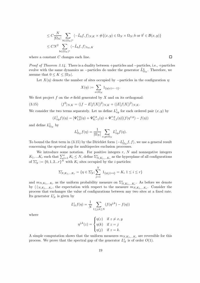
|ΩN |∑

b∈(ΩN )∗

〈−Lbf, f〉N,K ×#(x, y) ∈ ΩN × ΩN ; b or b′ ∈ B(x, y)

≤ CN2∑

b∈(ΩN )∗

〈−Lbf, f〉ΛN ,K

where a constant C changes each line.

Proof of Theorem 3.14. There is a duality between +particles and−particles, i.e., +particlesevolve with the same dynamics as −particles do under the generator LuΩN . Therefore, weassume that 0 ≤ K ≤ |ΩN |.

Let X(η) denote the number of sites occupied by −particles in the configuration η:

X(η) :=∑

x∈ΩN

1η(x)=−1.

We first project f on the σ-field generated by X and on its orthogonal:

(3.15) 〈f2〉N,K = 〈(f − E[f |X])2〉N,K + 〈(E[f |X])2〉N,K .We consider the two terms separately. Let us define L1

xy for each ordered pair (x, y) by

(L1xyf)(η) = [Ψx,y

1,0(η) + Ψx,y0,−1(η) + Ψx,y

−1,1(η)](f(ηx,y)− f(η))

and define L1ΩN

by

L1ΩN f(η) =

1

|ΩN |∑

x,y∈ΩN

L1xyf(η).

To bound the first term in (3.15) by the Dirichlet form 〈−L1ΩNf, f〉, we use a general result

concerning the spectral gap for multispecies exclusion processes.

We introduce some notation. For positive integers r, N and nonnegative integersK1, ...Kr such that

∑ri=1Ki ≤ N , define ΣrN,K1,...Kr

as the hyperplane of all configurations

of ΣrN := 0, 1, 2...rN with Ki sites occupied by the i-particles:

ΣrN,K1,...Kr= η ∈ ΣrN ;

N∑

j=1

1η(j)=i = Ki 1 ≤ i ≤ r

and mN,K1,...Kr as the uniform probability measure on ΣrN,K1,...Kr. As before we denote

by 〈·〉N,K1,...Kr , the expectation with respect to the measure mN,K1,...Kr. Consider theprocess that exchanges the value of configurations between any two sites at a fixed rate.Its generator LrN is given by

LrNf(η) =1

N

∑

1≤j,k≤N

(f(ηj,k)− f(η))

where

ηj,k(z) =

η(z) if z 6= x, y

η(k) if z = j

η(j) if z = k.

A simple computation shows that the uniform measures mN,K1,...Kr are reversible for thisprocess. We prove that the spectral gap of the generator LrN is of order O(1).

19

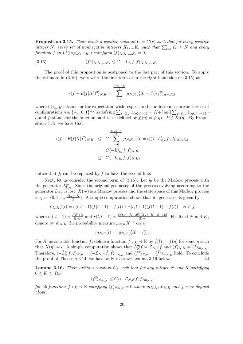
Proposition 3.15. There exists a positive constant C = C(r) such that for every positiveinteger N , every set of nonnegative integers K1, ...Kr such that

∑ri=1Ki ≤ N and every

function f in L2(mN,K1,...Kr) satisfying 〈f〉N,K1,...Kr = 0,

(3.16) 〈f2〉N,K1,...Kr ≤ C〈−LrNf, f〉N,K1,...Kr .

The proof of this proposition is postponed to the last part of this section. To applythe estimate in (3.16), we rewrite the first term of in the right hand side of (3.15) as

〈(f − E[f |X])2〉N,K =

|ΩN |−K

2∑

l=0

µN,K(X = l)〈f2l 〉ΛN ,K,l

where 〈·〉ΛN ,K,l stands for the expectation with respect to the uniform measure on the set ofconfigurations η ∈ −1, 0, 1ΩN satisfying

∑

x∈ΩN1η(x)=1 = K+l and

∑

x∈ΩN1η(x)=−1 =

l, and fl stands for the function on this set defined by fl(η) = f(η)−E[f |X](η). By Propo-sition 3.15, we have that

〈(f − E[f |X])2〉N,K ≤ C

|ΩN |−K

2∑

l=0

µN,K(X = l)〈−L1ΩN fl, fl〉ΛN ,K,l

= C〈−L1ΩNf, f〉N,K

≤ C〈−LΩNf, f〉N,K,

notice that fl can be replaced by f to have the second line.

Next, let us consider the second term of (3.15). Let ηt be the Markov process withthe generator LmΩN . Since the original geometry of the process evolving according to thegenerator LΩN is lost, X(ηt) is a Markov process and the state space of this Markov process

is χ := 0, 1, ..., |ΩN |−K2 . A simple computation shows that its generator is given by

LN,Kf(l) = r(l, l − 1)(f(l − 1)− f(l)) + r(l, l + 1)(f(l + 1)− f(l)) ∀l ∈ χ

where r(l, l− 1) = l(K+l)|ΩN | and r(l, l+ 1) = (|ΩN |−K−2l)(|ΩN |−K−2l−1)β

|ΩN | . For fixed N and K,

denote by mN,K the probability measure µN,KX−1 on χ:

mN,K(l) := µN,K(X = l).

For X-measurable function f , define a function f : χ→ R by f(l) := f(η) for some η suchthat X(η) = l. A simple computation shows that LmNf = LN,K f and 〈f〉N,K = 〈f〉mN,K .Therefore, 〈−LuNf, f〉N,K = 〈−LN,K f , f〉mN,K and 〈f2〉N,K = 〈f2〉mN,K hold. To concludethe proof of Theorem 3.14, we have only to prove Lemma 3.16 below.

Lemma 3.16. There exists a constant Cβ such that for any integer N and K satisfying0 ≤ K ≤ |ΩN |

〈f2〉mN,K ≤ Cβ〈−LN,Kf, f〉mN,Kfor all functions f : χ→ R satisfying 〈f〉mN,K = 0 where mN,K , LN,K and χ were definedabove.

20

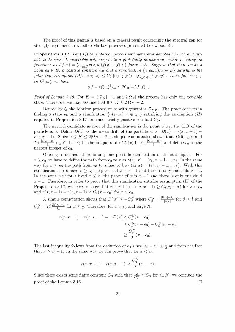
The proof of this lemma is based on a general result concerning the spectral gap forstrongly asymmetric reversible Markov processes presented below, see [4].

Proposition 3.17. Let (Xt) be a Markov process with generator denoted by L on a count-able state space E reversible with respect to a probability measure m, where L acting onfunctions as Lf(x) =

∑

y∈E r(x, y)(f(y) − f(x)) for x ∈ E. Suppose that there exists apoint e0 ∈ E, a positive constant C0 and a ramification γ(e0, x);x ∈ E satisfying thefollowing assumption (H): |γ(e0, x)| ≤ C0 [r(x, p(x))−∑

y∈s(x) r(x, y)]. Then, for every f

in L2(m), we have〈(f − 〈f〉m)2〉m ≤ 2C0〈−Lf, f〉m

Proof of Lemma 3.16. For K = 2|ΩN | − 1 and 2|ΩN | the process has only one possiblestate. Therefore, we may assume that 0 ≤ K ≤ 2|ΩN | − 2.

Denote by ξt the Markov process on χ with generator LN,K . The proof consists infinding a state e0 and a ramification γ(e0, x), x ∈ χn satisfying the assumption (H)required in Proposition 3.17 for some strictly positive constant C0.

The natural candidate as root of the ramification is the point where the drift of theparticle is 0. Define D(x) as the mean drift of the particle at x: D(x) = r(x, x + 1) −r(x, x − 1). Since 0 ≤ K ≤ 2|ΩN | − 2, a simple computation shows that D(0) ≥ 0 and

D([ |ΩN |−K2 ]) ≤ 0. Let e0 be the unique root of D(x) in [0, [ |ΩN |−K

2 ]] and define e0 as thenearest integer of e0.

Once e0 is defined, there is only one possible ramification of the state space. Forx ≥ e0 we have to define the path from e0 to x as γ(e0, x) = (e0, e0 +1, ..., x). In the sameway for x ≤ e0 the path from e0 to x has to be γ(e0, x) = (e0, e0 − 1, ..., x). With thisramification, for a fixed x ≥ e0 the parent of x is x− 1 and there is only one child x+ 1.In the same way for a fixed x ≤ e0 the parent of x is x + 1 and there is only one childx − 1. Therefore, in order to prove that this ramification satisfies assumption (H) of theProposition 3.17, we have to show that r(x, x + 1) − r(x, x − 1) ≥ C0(e0 − x) for x < e0and r(x, x− 1)− r(x, x+ 1) ≥ C0(x− e0) for x > e0.

A simple computation shows that D′(x) ≤ −CNβ where CNβ = |ΩN |−2β|ΩN | for β ≥ 1

4 and

CNβ = 2β 2|ΩN |−1|ΩN | for β ≤ 1

4 . Therefore, for x > e0 and large N,

r(x, x− 1)− r(x, x+ 1) = −D(x) ≥ CNβ (x− e0)

≥ CNβ (x− e0)− CNβ |e0 − e0|

≥CNβ2

(x− e0).

The last inequality follows from the definition of e0 since |e0 − e0| ≤ 12 and from the fact

that x ≥ e0 + 1. In the same way we can prove that for x < e0,

r(x, x+ 1)− r(x, x− 1) ≥CNβ2

(e0 − x).

Since there exists some finite constant Cβ such that 2CNβ

≤ Cβ for all N , we conclude the

proof of the Lemma 3.16.

21

Proof of Proposition 3.15. The idea of the proof consists in using the means of the math-ematical induction with respect to r. Assume r = 1. Then, the process is the uniformsymmetric simple exclusion process for which Quastel proved a spectral gap in [8].

Next, consider the general positive integer r. First of all, we suppose without lossof generality that K0 ≤ Ki for 0 ≤ i ≤ r where K0 := N − ∑r

i=1Ki. This implies thatK0 ≤ N

r+1 . For 0 ≤ i ≤ r, define π0 : ΣrN → 0, 1N as a function on the configurationspace which do not distinguish sites occupied by some particle:

π0(η) = ξ ∈ 0, 1N where ξ(j) =

1 η(j) = 0

0 otherwise.

For a function f in L2(mN,K1,...Kr) satisfying 〈f〉N,K1,...Kr = 0, define f0 as the conditionalexpectation of f with respect to the σ-field generated by π0. Then, similar to the proofof Theorem 3.14, we project f on this σ-field and on its orthogonal:

(3.17) 〈f2〉mN,K1,...Kr= 〈(f − f0)

2〉mN,K1,...Kr+ 〈f20 〉mN,K1,...Kr

.

We first consider the second term. The arguments are similar to the ones used in thesecond step of the proof of Theorem 3.14.

We may think f0 as a function defined on 0, 1N . The generator LrN acting on 0, 1Nis the generator of the usual uniform symmetric exclusion process for which Quastel [8]proved a spectral gap. Therefore, we have

〈f20 〉mN,K1,...Kr≤ 〈LrNf0, f0〉mN,K1,...Kr

≤ 〈LrNf, f〉mN,K1,...Kr.

We now turn to the first term of (3.17). For a subset B ⊂ ΛN := 1, ..., N such that#B = K0, define f0,B as a function on Σr−1

ΛN−B,K1,K2,...,Kr−1as follows:

f0,B(ξ) = f(ξB)− f0(ξB) ξ ∈ Σr−1

ΛN−B,K1,K2,...,Kr−1.

In this formula, ξB stands for the configuration η ∈ ΣrN,K1,K2,...,Krsuch that

η(i) =

0 if i ∈ B

j + 1 if ξ(i) = j.

With this notation, we rewrite the first term of (3.17) as follows:

〈(f − f0)2〉mN,K1,...Kr

=∑

B⊂ΛN

mN,K1,...Kr(η; η(i) = 0 for all i ∈ B)〈f20,B〉mN−K0,K1,...Kr−1.

The generator LrN acting on Σr−1ΛN−B,K1,K2,...,Kr−1

is the operator N−K0

NLr−1N−K0

. By theinduction assumption, there exists some constant Cr−1 such that

〈f0,B〉mN−K0,K1,...Kr−1≤ Cr−1〈Lr−1

N−K0f0,B, f0,B〉mN−K0,K1,...Kr−1

≤ Cr−1N

N −K0〈LrNf, f〉mN,K1,...Kr

.

By the assumption K0 ≤ Nr+1 , therefore we have N

N−K0≤ r+1

rand

〈f0,B〉mN−K0,K1,...Kr−1≤ Cr〈LrNf, f〉mN,K1,...Kr

for some constant Cr.

22

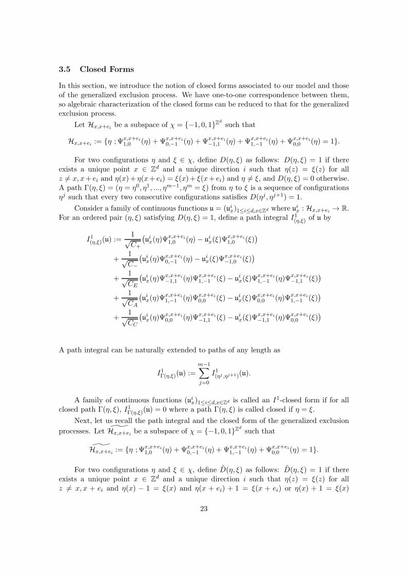
3.5 Closed Forms

In this section, we introduce the notion of closed forms associated to our model and thoseof the generalized exclusion process. We have one-to-one correspondence between them,so algebraic characterization of the closed forms can be reduced to that for the generalizedexclusion process.

Let Hx,x+ei be a subspace of χ = −1, 0, 1Zd such that

Hx,x+ei := η ; Ψx,x+ei1,0 (η) + Ψx,x+ei

0,−1 (η) + Ψx,x+ei−1,1 (η) + Ψx,x+ei

1,−1 (η) + Ψx,x+ei0,0 (η) = 1.

For two configurations η and ξ ∈ χ, define D(η, ξ) as follows: D(η, ξ) = 1 if thereexists a unique point x ∈ Zd and a unique direction i such that η(z) = ξ(z) for allz 6= x, x+ ei and η(x)+ η(x+ ei) = ξ(x)+ ξ(x+ ei) and η 6= ξ, and D(η, ξ) = 0 otherwise.A path Γ(η, ξ) = (η = η0, η1, ..., ηm−1, ηm = ξ) from η to ξ is a sequence of configurationsηj such that every two consecutive configurations satisfies D(ηj , ηj+1) = 1.

Consider a family of continuous functions u = (uix)1≤i≤d,x∈Zd where uix : Hx,x+ei → R.

For an ordered pair (η, ξ) satisfying D(η, ξ) = 1, define a path integral I1(η,ξ) of u by

I1(η,ξ)(u) :=1√C+

(

uix(η)Ψx,x+ei1,0 (η)− uix(ξ)Ψ

x,x+ei1,0 (ξ)

)

+1√C−

(

uix(η)Ψx,x+ei0,−1 (η)− uix(ξ)Ψ

x,x+ei−1,0 (ξ)

)

+1√CE

(

uix(η)Ψx,x+ei−1,1 (η)Ψx,x+ei

1,−1 (ξ)− uix(ξ)Ψx,x+ei1,−1 (η)Ψx,x+ei

−1,1 (ξ))

+1√CA

(

uix(η)Ψx,x+ei1,−1 (η)Ψx,x+ei

0,0 (ξ)− uix(ξ)Ψx,x+ei0,0 (η)Ψx,x+ei

1,−1 (ξ))

+1√CC

(

uix(η)Ψx,x+ei0,0 (η)Ψx,x+ei

−1,1 (ξ)− uix(ξ)Ψx,x+ei−1,1 (η)Ψx,x+ei

0,0 (ξ))

A path integral can be naturally extended to paths of any length as

I1Γ(η,ξ)(u) :=

m−1∑

j=0

I1(ηj ,ηj+1)(u).

A family of continuous functions (uix)1≤i≤d,x∈Zd is called an I1-closed form if for allclosed path Γ(η, ξ), I1Γ(η,ξ)(u) = 0 where a path Γ(η, ξ) is called closed if η = ξ.

Next, let us recall the path integral and the closed form of the generalized exclusion

processes. Let Hx,x+ei be a subspace of χ = −1, 0, 1Zd such that

Hx,x+ei := η ; Ψx,x+ei1,0 (η) + Ψx,x+ei

0,−1 (η) + Ψx,x+ei1,−1 (η) + Ψx,x+ei

0,0 (η) = 1.

For two configurations η and ξ ∈ χ, define D(η, ξ) as follows: D(η, ξ) = 1 if thereexists a unique point x ∈ Zd and a unique direction i such that η(z) = ξ(z) for allz 6= x, x + ei and η(x) − 1 = ξ(x) and η(x + ei) + 1 = ξ(x + ei) or η(x) + 1 = ξ(x)

23

and η(x + ei) − 1 = ξ(x + ei), and D(η, ξ) = 0 otherwise. A path Γ(η, ξ) = (η =η0, η1, ..., ηm−1, ηm = ξ) from η to ξ is a sequence of configurations ηj such that every twoconsecutive configurations satisfies D(ηj , ηj+1) = 1.

Consider a family of continuous functions (uix)1≤i≤d,x∈Zd where uix : Hx,x+ei → R. For

an ordered pair (η, ξ) satisfying D(η, ξ) = 1, define a path integral I2(η,ξ) by

I2(η,ξ)(u) :=

uix(η) if η(x)− 1 = ξ(x) and η(x+ ei) + 1 = ξ(x+ ei)

−uix(ξ) if η(x) + 1 = ξ(x) and η(x+ ei)− 1 = ξ(x+ ei).

A path integral can be naturally extended to paths of any length as

I2Γ(η,ξ)

(u) :=m−1∑

j=0

I2(ηj ,ηj+1)(u).

A family of continuous functions (uix)1≤i≤d,x∈Zd is called an I2-closed form if I2Γ(η,ξ)

(u) = 0

hold for all closed paths Γ(η, ξ).

Now, we construct one-to-one map from the set of I1-closed forms to the set of I2-closed forms. For an I1-closed form (uix)1≤i≤d,x∈Zd , define a family of continuous functions

(uix)1≤i≤d,x∈Zd as

uix(η) :=1√C+

uix(η)Ψx,x+ei1,0 (η) +

1√C−

uix(η)Ψx,x+ei0,−1 (η)

+1√CA

uix(η)Ψx,x+ei1,−1 (η) +

1√CC

uix(η)Ψx,x+ei0,0 (η),

then, (uix)1≤i≤d,x∈Zd is an I2-closed form. On the other hand, for an I2-closed form

(vix)1≤i≤d,x∈Zd , define a family of continuous functions (vix)1≤i≤d,x∈Zd as

vix(η) :=√

C+vix(η)Ψx,x+ei1,0 (η) +

√

C−vix(η)Ψx,x+ei0,−1 (η)

+√

CAvix(η)Ψx,x+ei1,−1 (η) +

√

CC vix(η)Ψx,x+ei0,0 (η)

−√

CE

[

(vix(ηx=1,x+ei=−1) + vix(η

x=0,x+ei=0))]

Ψx,x+ei−1,1 (η),

then, (vix)1≤i≤d,x∈Zd is an I1-closed form.

Let us introduce the notion of an I1-germ of closed form and an I2-germ of closedform. A family of continuous functions (gi)1≤i≤d (resp. gi) where gi : H0,ei → R is anI1(resp. I2)-germ of closed form if uix := τxgi is an I

1(resp. I2)-closed form.

Main theorem of this section is formulated as follows:

Theorem 3.18. For every I1-germ of closed form g, there exists a sequence of L2(νρ)-functions hn and constants (ci)1≤i≤d such that

gi = limn→∞

(ci

d∑

j=1

(U j)i +∇0,eiΓhn) in L2(νρ) for all 1 ≤ i ≤ d.

24

By the one-to-one correspondence between the I1-germ of closed form and the I2-germ of closed form and Cauchy-Schwartz inequality, in order to prove Theorem 3.18 wehave only to prove the next theorem:

Theorem 3.19. For every I2-germ of closed form g, there exists a sequence of L2(νρ)-functions hn and constants (ci)1≤i≤d such that

gi = limn→∞

(ci

d∑

j=1

(U j)i + ∇0,eiΓhn) in L2(νρ) for all 1 ≤ i ≤ d.

where Ui(η) = 1η(0)≥0,η(ei)≤0 and

∇0,eif(η) = Ψ0,ei1,0 (η)(f(η

0,ei)− f(η)) + Ψ0,ei0,−1(η)(f(η

0,ei)− f(η))

+ Ψ0,ei1,−1(η)(f(η

0=0,ei=0)− f(η)) + Ψ0,ei0,0 (η)(f(η

0=−1,ei=1)− f(η)).

Applying the method in [3], we can deduce this theorem since the proof depends onlyon the spectral gap estimates, which is proved by Theorem 1.8.1, and the fact that νρ istranslation invariant.

4 Proof of Theorem 2.2

The strategy of the proof is the same as given for liquid-solid system in [2]. The main stepis to establish the local ergodic theorem.

First, we consider a class of martingales associated with the empirical measure assimilar to Case 1. We also use the same notations: T , MH(t), πNt , QµN and Q∗ which aredefined in Section 3. In Case 2, we assume the gradient condition, C++C−−CA−2CE = 0,so the martingale MH(t) is rewritten as

MH(t) = 〈πNt ,H〉 − 〈πN0 ,H〉 −∫ t

0N−d

∑

x∈TdN

(∆NH)(x

N)τxh(ηs)ds

where h is a cylinder function defined by

h(η) = C+1η(0)=1 − C−1η(0)=−1

and ∆NH represents the discrete Laplacian of H:

(∆NH)(x

N) =

d∑

i=1

N2[H(x+ eiN

) +H(x− eiN

)− 2H(x

N)].

Following the same argument in Section 3, it is easy to prove that

limN→∞

PµN [ sup0≤t≤T

|MH(t)| ≥ δ] = 0

for every δ > 0, the sequence QµN , N ≥ 1 is weakly relatively compact and that everylimit points Q∗ is concentrated on absolutely continuous paths πt(du) = π(t, u)du withdensity bounded by 1 and -1 from above and below respectively: −1 ≤ π(t, u) ≤ 1.

25

From Theorem 6.1 stated below, there exists at most one weak solution of (2.5).Therefore, to conclude the proof of the theorem, it remains to show that all limit pointsof the sequence QµN , N ≥ 1 are concentrated on absolutely continuous trajectoriesπ(t, du) = π(t, u)du whose densities are weak solutions of the equation (2.5). For thispurpose, all we have to show is that

limN→∞

EµN [

∫ t

0N−d

∑

x∈TdN

(∆NH)(x

N)τxh(ηs)ds] = EQ∗ [

∫ t

0

∫

Td

(∆H)(u)P (π(s, u))ds]

where P is the function defined in (2.6).

First, we establish the local ergodic theorem which enables us to replace the samplemean of microscopic variables with their average under the equilibrium measure having amicroscopically defined sample density as its density-parameter. Let µNt ∈ P(χdN ) be the

probability distribution of ηt on χdN and let µN be the space-time average of µNt 0≤t≤T

defined by

µN =1

TNd

∑

x∈TdN

∫ T

0µNt · τ−1

x dt.

Then, we have that

Proposition 4.1 (local ergodic theorem). For every cylinder function f ,

limK→∞

lim supN→∞

EµN[|f0,K(η)− 〈f〉ηK(0)|] = 0

where f0,K = 1(2K+1)d

∑

|x|≤K τxf(η).

Proof. Let L be an operator on C defined by (Lf)(η) =∑

b∈(Zd)∗ Lbf(η), where (Zd)∗

stands for the set of all directed bonds. Following the method of the proof of Theorem 4.1in [2], it is easy to show that µNN is tight in P(χd) and an arbitrary limit µ ∈ P(χd)satisfies µ(Lf) = 0 for every cylinder function f . Moreover, by definition, µ is invariant

under spatial translations. Therefore, we have that support (µ) ⊂ −1, 0Zd ∪ 0, 1Zd . Itis known that the translation-invariant L-stationary measure on −1, 0Zd or 0, 1Zd isa superposition of Bernoulli product measures. Then, the law of large numbers concludesthe proposition.

Next, we need to prove that the sample density defined microscopically can be re-placed in the limit with the macroscopic one. We can use Young measures to complete itby the exactly same way as in [2]. Then, combining with these results, the main theoremwill be concluded. The details are omitted.

5 Proof of Theorem 2.3

In Case 3, since the hydrodynamic equation is the heat equation, the replacements whichare required in Case 2 are unnecessary. So, this is the easiest case to prove the hydrody-namic limit.

26

First, we consider a class of martingales associated with empirical measure again.Then, as in Case 2, the martingale MH(t) is rewritten as

MH(t) = 〈πNt ,H〉 − 〈πN0 ,H〉 − CE

∫ t

0〈πNs ,∆NH〉ds

+C+ − C−

2

∫ t

0N−d

∑

x∈TdN

1ηs(x)=0(∆NH)(

x

N)ds

where ∆NH represents the discrete Laplacian of H.

Following the same argument in Section 3 and 4, all we have to show is that

(5.1) limN→∞

EµN [

∫ t

0N−d

∑

x∈TdN

1ηs(x)=0ds] = 0.

With the notation defined in the last section, (5.1) is rewritten as

limN→∞

EµN[1η(0)=0 ] = 0.

Following the method of the proof of Theorem 4.1 in [2] again, it is easy to show that

µNN is tight in P(χd) and an arbitrary limit µ ∈ P(χd) satisfies µ(Lf) = 0 for everycylinder function f . Moreover, by definition, µ is invariant under spatial translations.Therefore, we have that support (µ) ⊂ −1, 1Zd and it concludes the theorem.

6 Weak Solutions of Nonlinear Parabolic Equations

In this section, we fix the terminology of weak solutions of parabolic equations and presentthe uniqueness of such equations. Hereafter φ : R → R is a strictly increasing and Lipschitzcontinuous function. We consider the Cauchy problem:

(6.1)

∂tρ(t, u) = ∆(φ(ρ(t, u)))(

=

d∑

i=1

∂2

∂u2iφ(ρ(t, u))

)

ρ(0, ·) = ρ0(·),and define weak solutions of this Cauchy problem.

Definition 6.1. Fix a bounded initial profile ρ0 : Td → R. A measurable function ρ ≡ρ(t) = ρ(t, u) ∈ C([0, T ],M(Td))∩L2([0, T ]×Td) is a weak solution of the Cauchy problem(6.1) if for every function H : Td → R of class C2(Td) and for every 0 ≤ t ≤ T

∫

Td

H(u)ρ(t, u)du =

∫ t

0ds

∫

Td

φ(ρ(s, u))∆H(u)du +

∫

Td

H(u)ρ0(u)du.

We prove the uniqueness of weak solutions in this class.

Theorem 6.1. Fix a bounded measurable function ρ0 : Td → R. There exists at most one

weak solution of the parabolic equation (6.1).

Proof. We can apply the proof of Theorem A.2.4.4 in [3] straightforwardly.

27

Acknowledgement

The author would like to thank Professor T. Funaki for helping her with valuable sugges-tions.

References

[1] P. Collet, F. Dunlop, D. Foster, T. Gobron, Product measures and frontdynamics for solid on solid interfaces, J. Stat. Phys., 89 (1997), 509–536.

[2] T. Funaki, Free boundary problem from stochastic lattice gas model, Ann. Inst. H.Poincare, Probab. Statis., 35 (1999), 573–603.

[3] C. Kipnis and C. Landim, Scaling Limits of Interacting Particle Systems, 1999,Springer.

[4] C. Kipnis, C. Landim and S. Olla, Hydrodynamic limit for a nongradient system:The generalized symmetric exclusion process, Comm. Pure Appl. Math., 47 (1994),1475–1545.

[5] C. Kipnis, and S.R.S. Varadhan, Central limit theorem for additive functionalsof reversible Markov processes and applications to simple exclusion, Comm. Math.Phys., 104 (1986), 1–19.

[6] J. Quastel, Diffusion of color in the simple exclusion process, Comm. Pure Appl.Math., 45 (1992), 623–679.

[7] H. Spohn, Large Scale Dynamics of Interacting Particles, 1991, Springer.

28