The domino shuffling height process and its hydrodynamic limit

The domino shuffling height process and itshydrodynamic limit

Xufan ZhangBrown University

Providence RI 02912 USA

Abstract

The famous domino shuffling algorithm was invented to generate the domino tilingsof the Aztec Diamond Using the domino height function we view the domino shufflingprocedure as a discrete-time random height process on the plane The hydrodynamiclimit from an arbitrary continuous profile is deduced to be the unique viscosity solutionof a Hamilton-Jacobi equation ut + H(ux) = 0 where the determinant of the Hessianof H is negative everywhere The proof involves interpolation of the discrete processand analysis of the limiting semigroup of the evolution In order to identify the limitwe use the theories of dimer models as well as Hamilton-Jacobi equations

It seems that our result is the first example in d gt 1 where such a full hydrodynamiclimit with a nonconvex Hamiltonian can be obtained for a discrete system We alsodefine the shuffling height process for more general periodic dimer models where weexpect similar results to hold

Contents

1 Introduction 2

2 General setup 521 Dimer model on a periodic bipartite graph 522 Height function 623 Local moves 724 Shuffling height process 9

3 The main result 1231 The specific example 1232 Hydrodynamic limit 14

1

arX

iv1

808

0740

9v3

[m

ath

PR]

8 M

ay 2

019

4 Smoothing out the height process 1641 Useful properties of the height process 1642 Smoothing out the height process spatially 1743 The space of continuous evolutions 2144 Smoothing out the height process temporally 23

5 Limit points 2851 Precompactness 2852 Characterization of limit points 29

6 Equilibrium measures 3361 Construction of Gibbs measures 3362 Evolution at equilibrium 3663 More on limit points 40

7 Viscosity solution 42

8 Remarks 46

A Proof of Proposition 22 46

B Local interpolations for constructing Sn 47

1 Introduction

The dimer model which consists of the weighted perfect matchings on graphs is a well-studied model in mathematical physics The domino model is the dimer model on a (possiblyinfinite) region of the Z2 lattice Alternatively it can be thought of as tiling a region of thesquare grid exactly by 1times 2 and 2times 1 dominoes For a comprehensive survey on the subjectof dimer models see [16] Necessary knowledge will be reviewed in the paper

The domino shuffling is a discrete-time random dynamics operating on the domino modelintroduced originally by Elkies et al in [6] to compute the generating function of dominotilings of a specific family of graphs called Aztec Diamonds with periodic weights In partic-ular the domino shuffling provides a simple algorithm to generate the uniform measure oftilings of Aztec Diamonds and led to the first rigorous proof of the famous Artic Circle The-orem by Jockusch et al([10]) that describes the asymptotic shape of the central sub-regionof a random tiling

The domino shuffling seemed quite mysterious the way it was presented in [6] initiallyPropp([21]) later gave a much clearer explanation using a procedure called urban renewalor spider move which also allows natural generalizations to different graphs This is theapproach we will take to define the shuffling dynamics in Section 2 As it turns out this alsonaturally converts the shuffling dynamics into a random height process which we shall callthe shuffling height process The height process is a (2 + 1)-dimensional evolution which is

2

discrete in both space (2-dimensional) and time (1-dimensional) The purpose of this paperis to prove that when rescaling both space and time parameters by n and starting nearby anarbitrary continuous profile (subject to certain legality requirement) as nrarrinfin the heightprocess evolves according to a first-order nonlinear Hamilton-Jacobi equation

ut +H(ux) = 0 (11)

where in the case of uniform shuffling the Hamiltonian is given by

H(ρ1 ρ2) =4

πcosminus1

(1

2cos(πρ2

2

)minus 1

2cos(πρ1

2

))

The convergence is uniform in any compact subset of the spacetime A subtlety is that thePDE develops shocks even starting from a smooth profile so we need to consider a specificweak solution called the viscosity solution

Before sketching the proof we would like to mention some other works on domino shuf-fling Johansson([11]) and Nordenstam([20]) related the domino shuffling on the Aztec Di-amond to a determinantal point process As a result they were able to prove that underappropriate rescaling the boundary of the arctic circle converges to the Airy process andthe turning point converges to the GUE minor process In 2014 Borodin and Ferrari([2])pushed this idea further where several different (2 + 1)-dimensional interacting particle sys-tems and random tiling models were connected through systems of non-intersecting linesThese models are believed to belong to the Anisotropic KardarParisiZhang (AKPZ) univer-sality class which means that the speed function H in the hydrodynamic limit (11) has theproperty that the determinant of its Hessian is negative The domino shuffling dynamicsis in particular one of them with the connection explained by the same authors([3]) laterin more detail Recently Chhita and Toninelli([4]) analyzed the speed and fluctuation ofdomino shuffling on the 2-periodic Z2 lattice and demonstrated a ldquorigidrdquo stationary statewhere the fluctuation is O(1)

Many of the works above focus on a specific type of region or initial condition In termsof hydrodynamic limits starting from a more general profile the first rigorous result inthe context above was obtained in 2017 by Legras and Toninelli([29][19]) They analyzedanother stochastic interface growth model from [2] which can be viewed as a continuous-time dynamics on lozenge tilings (the dimer model on the hexagonal lattice) In this casedifferent from the domino shuffling dynamics updates at a point can depend on informationarbitrarily far away and the speed function is unbounded As a result the hydrodynamiclimit is proved either up to the first shock time or when the initial profile is convex

We also want to mention some background in hydrodynamic limit theory One generalapproach to the hydrodynamic limit of discrete systems is to first make an educated guessabout the form of the limit based on a local-equilibrium heuristic that is assuming thesystem is locally at equilibrium almost everywhere for all time This often leads to anexplicit PDE which serves as a guide When the PDE theory provides a characterizationof a unique (weak) solution we can try to adapt the form of the solution to the discretesystem For example when we are dealing with the symmetric nearest neighbor simple

3

exclusion process as discussed in Chapter 4 of the classical reference [18] the hydrodynamiclimit is expected to be the heat equation whose unique solution can be characterized byan integral equation Therefore one wants to show that starting from a particular initialprofile the Riemann sum based on the empirical measure of the discrete system converges toan integral This then becomes a classical problem in probability of showing the convergenceof measures First one uses Prokhorovrsquos theorem to show that every sequence of measureshas a subsequential limit Then one uses specific knowledge about the discrete system toprove that any subsequential limit must agree with the desired integral equation in this caseusing martingale techniques

In the case when the expected PDE is a Hamilton-Jacobi equation the PDE theory ismore complicated When the speed function H is convex or the initial profile is convexthe unique viscosity solution can be written down in a variational form using either theHopf-Lax formula or Hopf formula ([8]) Certain exclusion processes do have such a PDE asthe limit and one proof strategy consists of finding a corresponding microscopic variationalformula for the discrete system and showing the convergence of this formula to the continuousone See for example the works by Seppalainen([24]) and Rezakhanlou([23]) Also the Hopfformula is used in [19] to prove the limit starting from a convex profile

However since the AKPZ property exactly means that the speed function H is neitherconvex nor concave an explicit variational formula for the unique solution is not available(Evans([8]) gave a general representation formula but it is not clear how to relate it to thesediscrete systems) The seminal work [22] of Rezakhanlou in 2001 provided an approachin the context of certain continuous-time exclusion processes Just as in the case of simpleexclusion processes one would like to prove the convergence of empirical measures Howeverthe unique viscosity solution of the Hamilton-Jacobi equation has a peculiar characterizationIt involves comparing the current solution to a family of arbitrary smooth functions atall spacetime locations Therefore the empirical measures which we want to demonstrateconvergence of need to encode the evolution from not just one initial condition but allpossible initial conditions starting from an arbitrary time ie as a discrete ldquosemigrouprdquoA priori to encode this much information the space of the resulting probability measureswould be too large ie inseparable to apply Prokhorovrsquos theorem The key observation ofRezakhanlou is that if the discrete system satisfies certain properties the space of probabilitymeasures can be made separable In [22] the full hydrodynamic limit of a family of exclusionprocesses in d = 1 was established with a nonexplicit Hamiltonian It seems that our result isthe first example in d gt 1 where such a full hydrodynamic limit with a nonconvex Hamiltonianhas been obtained for a discrete system

Another issue is that the evolution of the discrete system needs to be properly interpolatedto be comparable to the evolution of the PDE and more importantly to keep the space ofprobability measures separable We carry out the interpolation of the domino shuffling inSection 4 The interpolation in [22] is straightforward but it takes extra work in our casedue to the differences of the models A convenience for us however is that the topologycan be taken to be the uniform topology instead of the Skorohod topology This makes theargument more transparent

4

In Section 6 utilizing the dimer theory we identify the Gibbs measures of domino tilingsas equilibrium measures of the shuffling process and deduce the hydrodynamic limit startingfrom a flat initial condition (Notice that we do not need the uniqueness of the dimer Gibbsmeasures) This allows us to determine the full hydrodynamic limit in Section 7 Whileusing the general theory of viscosity solutions we have to take care of the boundedness ofthe spatial gradient imposed by our model

The rest of the paper is outlined as follows In Section 2 we will provide some backgroundinformation about the dimer model and the dimer shuffling height process is defined in ageneral manner We also establish a list of lemmas that are useful later The specific set-upfor the remainder of the paper and the precise statement of the theorem are presented inSection 3 In Section 5 we apply Prokhorovrsquos theorem and the generalized Arzela-Ascolitheorem to deduce the precompactness of the sequence of the empirical measures on discreteldquosemigroupsrdquo and also prove some additional properties about the subsequential limits tobe used later In particular the limits are bona fide semigroups Section 8 briefly discussessome other examples of the dimer shuffling process and possible extensions

2 General setup

21 Dimer model on a periodic bipartite graph

To start with consider a Z2-periodic bipartite graph G = (VE) embedded in the planewhere the vertices in each fundamental domain are colored black and white in a particu-lar way such that the whole graph is invariant under the natural Z2-translation action Tmatching fundamental domains One primary example will be the graph shown in Figure 1Also define Gn = G(nZ)2 as the quotient graph embedded on a torus

Figure 1 The bipartite graph with vertices Z2 and one fundamental domain drawn Thevertices in this figure should be considered lying on the dual lattice of Figure 7

A dimer covering on a bipartite graph is a subset of the edges E that form a perfectmatching among the vertices V A chosen edge is called a dimer We assign a nonnegativeweight w(e) to each edge e invariant under T Then on finite graphs G1 and Gn we can

5

define a Boltzmann probability measure on the set of dimer coverings M

micro[M isinM] =1

Z

prodeisinM

w(e)

where Z =sum

MisinMprod

eisinM w(e) is the partition function Notice that the measure is invariantunder a gauge transformation which means multiplying all edge weights incident to a vertexby a positive constant

This definition of course does not make sense on G but we can always take a sequenceof Boltzmann measures on Gn with nrarrinfin and any weakly convergent subsequence (whichis guaranteed to exist by Prokhorovrsquos theorem) will yield a limiting Gibbs measure on Gwhose finite dimensional distributions are the limit along the convergent subsequence

22 Height function

A flow on a graph is an assignment of real numbers to the directed edges such that edgeswith opposite directions are assigned opposite numbers Given a dimer covering M on Gwe can think of it as a white-to-black flow [M ] where each white-to-black edge is assignedeither 1 or 0 If we fix some reference covering M0 then [M ]minus [M0] is a divergence-free flow(the net flow into each vertex is equal to 0) which induces a gradient flow on the dual graphIn other words we can attribute a height function hM defined on the faces to the coveringM by first stipulating that one base face has height 0 and assigning neighboring faces theirheights as follows When we cross an edge the height will increase by the net amount offlow on that edge from left to right

This height function hM is well defined on a planar graph up to an additive constantand it is clear that given the reference covering we can recover the dimer covering M fromits height function hM If the graph is embedded on a torus such as Gn defined above hMis still well-defined locally but is treated as a multi-valued function globally Suppose hMincreases by x as we move towards the right once around the torus back to the same faceand increases by y as we move up once around the torus we say that hM or the coveringM itself has height change (x y) Since hM is well defined locally (x y) does not depend onthe choice of cycles as long as they have homology (1 0) and (0 1) respectively

The set of all possible height changes on G1 = GZ2 plays an important role in dimertheory Their convex hull is called the Newton polygon associated to G which roughlyspeaking contains exactly all possible ldquoslopesrdquo on G ([17])

A different reference covering M prime0 will define a different height function for M The

difference is determined by [M0]minus [M prime0] which is independent of the covering M of interest

Therefore given two coverings M and M prime the function hM minus hM prime does not depend on thechoice of reference covering

A nice property about these height functions is that they have a lattice structure by takingpointwise maximum or minimum This fact was briefly mentioned in [5] in the context ofdomino tilings Here we give a proof in the above setting

6

Lemma 21 (Lattice property) Fixing a reference covering M0 on G if hM and hM prime areboth height functions with integer values then both hM andhM prime and hM orhM prime are dimer heightfunctions where and denotes pointwise minimum and or denotes pointwise maximum

Proof WLOG suppose g = hM or hM prime We first prove by contradiction that the followingscenario can never happen there is be an edge e separating two faces f1 and f2 such thatg(f1) = hM(f1) gt hM prime(f1) and g(f2) = hM prime(f2) gt hM(f2) Let us assume that when we crosse from f1 to f2 the white vertex is on the left If e isinM0 a dimer height function either staysthe same or decreases by 1 going from f1 to f2 Then we must have hM(f2) ge hM(f1)minus 1 gehM prime(f1) ge hM prime(f2) a contradiction Similarly if e isinM0 a dimer height function either staysthe same or increases by 1 going from f1 to f2 Then hM prime(f1) ge hM prime(f2) minus 1 ge hM(f2) gehM(f1) again a contradiction

Now suppose g is not a dimer height function One possible obstacle is that for someedge e separating two faces f1 and f2 g(f1) minus g(f2) is not one of the allowed dimer heightchanges across e Then the scenario above must happen which is impossible

Another possible obstacle is when the value of g changes at least four times circlingaround a vertex v (Obviously g has to change even number of times circling around anyvertex) On the other hand any dimer height function must change either zero or two timescircling around v Also if e0 is the unique edge in M0 that connects v a dimer height functionthat changes two times circling around v must change its value across e0 This implies thatout of the four value changes for g around v at least one change corresponds to the scenariomentioned before which is again impossible

The last possible obstacle is when the value of g changes exactly two times circling arounda vertex v but neither of them happens at e0 borrowing the notations from above Sincethe scenario mentioned at the beginning is impossible those two changes must have one ofthem coinciding with hM and the other coinciding with hM prime Therefore both hM and hM prime

must both change across e0 with the same net increase But since g = hM or hM prime g mustalso change across e0 a contradiction

23 Local moves

Now we define two types of local moves for the dimer model vertex contractionexpansionand the spider move These first appeared in [21] and were also studied in [9 26] Theselocal moves happen at two different levels One level is a local modification of the weightedbipartite graph and another level is a possibly random mapping of dimer coverings on thegraph

Vertex contractionexpansion on the graph level involves either shrinking a 2-valentvertex and its two incident edges into a single vertex or its reversal See Figure 2 Assumethat the three vertices involved are all distinct Before shrinking we first perform a gaugetransformation to make both edge weights equal to 1 During expansion on the other handsimply assign both edges weight 1

On the dimer level given a dimer covering before contraction we simply delete thedimer incident to the deleted middle vertex and keep the rest of the dimer covering after

7

Figure 2 Vertex contractionexpansion move

1 1

contraction For expansion we keep the covering and match the added middle vertex withthe unmatched side

The spider move is the more interesting case See Figure 3 for an illustration

Figure 3 Spider move on graph level

1 1

1 1

Start with a quadrilateral face with a top-left black vertex such that all four vertices aredistinct On the graph level first insert four tentacles at the corners The four tentacles areassigned weight 1 The other four weights are assigned as follows

A =c

ac+ bd B =

d

ac+ bd C =

a

ac+ bdD =

b

ac+ bd (21)

For the spider move with the opposite coloring first perform vertex expansion at four cornersand then implement the spider move on the internal face For the reversal with the originalcoloring perform the opposite-coloring spider move on the internal face and shrink the four2-valent edges Hence we only call the move in Figure 3 the spider move

On the dimer level we keep all the dimers that are not one of the four internal edges Thendepending on whether each of four original vertices were matched externally or internallywe make some choices in order to complete a dimer covering See Figure 4 for some of thecases

In the first row of Figure 4 a choice is made between the two possibilities according tothe ratio between their total weights The two horizontal dimers are chosen with probability

ACAC+BD

and the two vertical dimers are chosen with probability BDAC+BD

Many variants ofthe following statement appeared in the literature([9 21 26]) and we will include a proofat the end for completeness

Proposition 22 For any finite bipartite graph H embedded on a torus the local movespreserve the Boltzmann measure of dimer coverings on H in the sense that applying a local

8

Figure 4 Spider moves on the dimer level Only the first row has randomness In the secondrow we omitted three other symmetric cases

or

move to the Boltzmann measure on H results in the Boltzmann measure on the new graphH prime

24 Shuffling height process

The following is not a precise definition but rather a general description of the type ofprocess we are considering

First we consider a global operation where we choose a local move on G or Gn andperform it at all T -periodic counterparts simultaneously requiring that the edges involveddo not overlap with each other The spider moves at different locations are independent interms of their randomness See Figure 8 for an example

By Proposition 22 such a global operation still preserves the Boltzmann measure sincewe can consider it as performing the local moves sequentially It is also well defined on Gas we can perform the local moves in the increasing order of their distance from the originso that every finite region of G will be determined after some finite number of local moves

Second we want to compare the height functions before and after a local move Giventhe reference covering M0 and a height function hM before a local move we may choose(in most cases there is a natural choice) the reference covering after the local move to bedeterministically one of the possible outcomes of the local move applied to M0 This definesa new height function hM prime for the random outcome M prime

Lemma 23 With the choice above of the reference covering on G hM prime agrees with hM at

9

every face except the inner face of the spider move (up to a global additive constant which ismade zero) where M prime is an outcome of M after a local move

For a moment let us forget about the precise embedding When we say hM prime agrees withhM at a face we mean that the heights defined at the combinatorially corresponding facesagree since no face is created or destroyed

Proof We can relate the heights at different faces as in Figure 5 Since we assume that allvertices involved in the local moves are distinct the dimer configuration along the dottedpaths drawn remains the same Therefore the height on the surrounding faces can be madeinvariant before and after the local move Then the height at every other face also staysunchanged except the middle one in the spider move

Figure 5 Paths in dual graphs

A consequence of Lemma 23 is that during a global operation the heights of all thefaces except the inner faces of spider moves can be kept unchanged since such is true afterevery local move This is the reason why we will be able to discuss the evolution of heightfunctions Also in this case we will choose the same new reference dimer for each localmove That is we can assume that the reference covering remains T -periodic after a globaloperation

When there are two dimer coverings M1 and M2 on G we can perform a local move ora global operation on them simultaneously The only requirement is that they are coupledso that each pair of corresponding faces during a spider move share the same randomnessThen we have the following ldquomonotonicityrdquo lemma

Lemma 24 (Monotonicity) With the same choice of reference covering on G as in Lemma 23if hM1 ge hM2 at each corresponding face before a local move then hM prime

1ge hM prime

2still holds af-

terwards where M prime1 and M prime

2 are the coupled results of the local move performed on M1 andM2 respectively

Proof The heights of the faces do not change in vertex contractionexpansion so there isnothing to prove there

10

It suffices to consider hM1 minus hM2 and hM prime1minus hM prime

2 since they do not depend on the choice

of reference covering By assumption hM1 minus hM2 ge 0 By Lemma 23 we can assume thatfor both hM1 and hM2 the heights at all other faces stay the same except the internal faceof the spider move denoted as f

Therefore we have hM prime1minushM prime

2ge 0 at all faces except f Suppose the statement is wrong

then hM prime1minushM prime

2lt 0 at f By considering the flow [M prime

1]minus [M prime2] the only case this can happen

is shown in Figure 6 where the green vertical dimers are in M prime2 and the red horizontal dimers

are in M prime1 This cannot happen since we assumed that they are coupled at f during the spider

move

Figure 6 A local configuration of two dimer coverings

Now to obtain a tractable height process we make a strong assumptionAssumption After a particular choice of sequence of global operations being performed

on Gn (resp G) the resulting graph coincides with Gn (resp G) in terms of the actualembedding with combinatorially corresponding faces matching each other and the edgeweights are also the same up to gauge transformations

Another assumption is that the reference dimer covering also remains the same This isnot necessary because there are only finitely many T -periodic coverings so we can make thistrue by running longer time if necessary given the assumption above

If the assumption above is true we call one iteration of such a sequence of global opera-tions a shuffle and the corresponding height evolution a shuffling height process

The assumption might seem very strong The specific example that we will analyze isthe one in Figure 1 But already in Z2 lattice by increasing the size of the fundamentaldomain some special phenomena in the steady state fluctuation are discovered in [4]

The reason why we introduced this process in this more general manner is first the exis-tence of the hydrodynamic limit of any such process can be obtained by a similar approacheven though the specific PDE might be hard to compute and second the necessary lemmaslisted above and their proofs do not assume much about the specific graph structure so itseems more natural to state them independently

11

3 The main result

31 The specific example

Now we turn to the simplest example where a shuffling height process can be defined the1-periodic domino tiling model in Figure 1

We assume that the vertical edges have weightradica and the horizontal edges have weight 1

as any other choice of positive weights with the same fundamental domain is gauge equivalentto this one By convention in the literature we choose the reference flow [M0] in the initialgraph to be 14 on each edge We define the height function h on the faces which arelabeled by coordinates in Z2 With this coordinate the graph is periodic under the actionT generated by translations (2 0) and (0 2)

We assume that initially the face at (0 0) has a top-left black vertex We call faces (i j)with i + j even even faces and otherwise odd faces Also we multiply the heights by 4 sothat all of them are integers This is the height function of domino tilings defined in [27]Figure 7 shows a picture in terms of dominoes

Figure 7 A domino tiling on a so-called Aztec diamond region with heights labeled Thevertices lie on the dual lattice of Figure 1

To be clear when we speak of an ldquoedgerdquo we always refer to an edge on the primal graphas in Figure 1 etc By definition of the height function when we cross an edge with a whitevertex on the left the height either increases by 3 or decreases by 1 Therefore once we fixthe height of face (0 0) modulo 4 all other faces are determined modulo 4

The shuffling procedure is just the domino shuffling from [6] Propp [21] rephrased thisshuffling procedure in terms of the local moves described in Section 23 By our definitiona shuffle consists of the following steps

1 Perform a spider move at all even faces (i j) (these are two T -periodic families of localmoves)

2 Perform vertex contraction at all 2-valent vertices

12

3 Perform a spider move at all odd faces (i j)


See Figure 8 for one iteration By formula (21) after Step 1 the horizontal edge weights

become 11+a

and the vertical edge weights becomeradica

1+a So up to gauge transformations the

edge weights remain the same after Step 2 and after Step 4 as well By viewing the referenceflow [M0] as a convex combination of four different integer coverings each consisting of asingle type of edges [M0] also remains 14 on all horizontal and vertical edges Thereforethe assumption for a shuffling height process is satisfied

Figure 8 One domino shuffle with a fixed fundamental domain labeled Each step consistsof several T -periodic families of local moves

Consider the height at certain even face (i j) By Lemma 23 it only gets modified atStep 1 of a shuffle since that is the only time when that face undergoes a spider move Asmall inconvenience is that the height module 4 changes after a shuffle To compensate forthat from now on we subtract all heights by 2 after every shuffle This amounts to addinga constant drift to the hydrodynamic limit which does no harm Since the only relevantfaces during a spider move are the neighboring ones we can list all the possible outcomes at(i j) after a shuffle in Table 1 We see that the height at (i j) is nonincreasing and staysthe same modulo 4 The same table also describes the height evolution at an odd face (i j)where the left column represents the height after Step 2 In other words the entire heightprocess can be defined using the local rules described in Table 1 without mentioning dimers

13

Table 1 The height evolution at an even face (i j) during a shuffle

Local heights centered at (i j) The height at (i j) after the shuffle

h+ 1hminus 1 h hminus 1 hminus 4

hminus 3

hminus 3hminus 1 h hminus 1 hminus 4

h+ 1

h+ 1 h with probability a1+a

hminus 1 h hminus 1h+ 1 hminus 4 with probability 1

1+a

h+ 1hminus 1 h h+ 3 h

h+ 1

h+ 1h+ 3 h hminus 1 h

h+ 1


hminus 3

h+ 1h+ 3 h h+ 3 h

h+ 1

32 Hydrodynamic limit

To state a hydrodynamic limit result on the height evolution we need to introduce a timeparameter t Suppose the initial condition at t = 0 is the height function of certain dimercovering on G which is a function Z2 rarr Z as defined previously the dynamics is that ashuffle happens at t = 1 2 3 This defines a random process h Z2 times N rarr Z whereh(x t) denotes the height at face x and time t A priori the spatial function h(middot t) for anyt is a domino height function As mentioned before h(x middot) is nonincreasing Furthermorewe require that h(0 0) equiv 0 (mod 4) This immediately determines all h(x t) (mod 4) Wewill call such height function h(middot t) admissible

The underlying probability space Ω consists of a collection of iid Bernoulli random vari-ables at each (x t) isin Z2 times N which take value 1 with probability 1

1+aand value 0 with

probability a1+a

In particular given ω isin Ω ω(x t) dictates the randomness of a spider move

14

that happens at face x and time tDefine the space of asymptotic height functions Γ to be the set of all 2-spatially-Lipschitz

functions from R2 to R which in this paper means

|f(x)minus f(y)| le 2 |xminus y|infin

where | middot |p is the `p normThe choice of Γ comes from the Newton polygon as defined in Section 22 In this case

the (rescaled) Newton polygon bounds the region U = x |x|1 le 2 and a differentiablefunction is in Γ iff its gradient lies in U See Lemma 72 for a similar statement

Now suppose we are given some g isin Γ and a sequence of initial conditions (hn(middot 0))nisinNapproximating g What we mean exactly is that (hn(middot 0)) is a sequence of admissible heightfunctions random or not independent or not such that

limnrarrinfin

E sup|x|1leR

∣∣∣∣ 1nhn(bnxc 0)minus g(x)

∣∣∣∣ = 0 (31)

for every finite R gt 0 and the expectation E is taken over the probability space Ω0 of theinitial condition (hn(middot 0))nisinZgt0

The height evolution of (hn) is governed by the single probability space Ω This meansimplicitly that the randomness of a spider move at (x t) is coupled for all hn

Now we are ready to state the hydrodynamic limit

Theorem 31 We have for every R gt 0

limnrarrinfin

E sup|x|1leRtleR

∣∣∣∣ 1nhn(bnxc bntc)minus u(x t)

∣∣∣∣ = 0 (32)

where u R2 times Rge0 rarr R is the unique viscosity solution ofut +H(ux) = 0

u(x 0) = g(x)(33)

H is defined on U by

H(ρ1 ρ2) =4

πcosminus1

(a

1 + acos(πρ2

2

)minus 1

1 + acos(πρ1

2

)) (34)

ut = partupartt

and ux denotes the spatial gradient of u

The precise definition of viscosity solutions is delayed to Section 7

Remark Notice that H is continuous on U One can compute the determinant of the Hessianof H to be

minus

(aπ(cos(πρ12

)+ cos

(πρ22

))(a+ 1)2 minus

(cos(πρ12

)minus a cos

(πρ22

))2

)2

which is negative in the interior of U The result here is for the shuffling in the plane It can be replaced by a torus or cylinder

and the formula remains the same

15

4 Smoothing out the height process

The goal of this section is to embed the height process h(s t) in a suitable space which asshown later also contains the semigroup solving the PDE Since h is discrete in both spaceand time we need to extend it to a continuous process

41 Useful properties of the height process

We first take a closer look at our height process h(x t) Let Φ denote the space of alladmissible height functions which are domino height functions whose value at (0 0) is 0(mod 4) The following lemma is rephrasing Lemma 21

Lemma 41 (Lattice property) If ϕ1 ϕ2 isin Φ then ϕ1 and ϕ2 isin Φ and ϕ1 or ϕ2 isin Φ

Define h(x tϕ ω) as the height at position x and time t of the deterministic heightprocess with an initial configuration h(middot 0) = ϕ isin Φ and Bernoulli mark ω isin Ω

Since ϕ isin Φ is well defined up to a global additive constant that is a multiple of 4 forall k isin Z

h(x tϕ+ 4k ω) = h(x tϕ ω) + 4k (41)

The following ldquomonotonicityrdquo lemma is the deterministic version of Lemma 24

Lemma 42 (Monotonicity) Given ϕ1 ϕ2 isin Φ if ϕ1 le ϕ2 then h(middot tϕ1 ω) le h(middot tϕ2 ω)for all t isin N

Now we state a simple but crucial lemma which states that information propagates atlinear speed This can also be easily generalized to other shuffling height processes

Lemma 43 (Linear propagation) Given ϕ1 ϕ2 isin Φ and x isin Z2 if ϕ1(y) = ϕ2(y) for all ysuch that |xminusy|1 le R then h(y tϕ1 ω) = h(y tϕ2 ω) for all y such that |xminusy|1 le Rminus2t

Proof During each shuffle there are two rounds of height updates In the first step alleven faces (i j) get modified But since ω is given the new height at (i j) is just a functionof the heights of its four neighbors Similarly in the third step heights at odd faces (i j)are updated according to its four neighbors Therefore the new height at any face x aftera shuffle is just a function of original heights at y where |y minus x|1 le 2 Now the statementfollows by an induction on t

Combing the few statements we deduce a ldquolocalizationrdquo property of shuffling heightprocesses

Proposition 44 (Localization) Assume k isin N

1 Given ϕ1 ϕ2 isin Φ and x isin Z2 if |ϕ1(y)minus ϕ2(y)| le 4k for all y such that |xminus y|1 le Rthen |h(y tϕ1 ω)minus h(y tϕ2 ω)| le 4k for all y such that |xminus y|1 le Rminus 2t

16

2 Given ϕ1 ϕ2 isin Φ if |ϕ1(y)minusϕ2(y)| le 4k for all y then |h(y tϕ1 ω)minush(y tϕ2 ω)| le4k for all y

Proof Let ϕ3 = ϕ1or (ϕ2 +4k) which is admissible by Lemma 41 Since ϕ1(y) le ϕ2(y)+4kfor all y such that |xminus y|1 le R we have ϕ3(y) = ϕ2(y) + 4k for all such y By Lemma 43h(y tϕ3 ω) = h(y tϕ2 + 4k ω) for all y such that |xminus y|1 le Rminus 2t Therefore for all suchy

h(y tϕ1 ω) le h(y tϕ3 ω)

= h(y tϕ2 + 4k ω)

= h(y tϕ2 ω) + 4k (by (41))

The other inequality can be proved similarly so the first statement holds The secondstatement follows by taking R =infin

Another property of the height process is that the vertical drift speed is linearly bounded

Lemma 45 (Vertical speed bound) For any ϕ isin Φ x isin Z2 and t isin N

ϕ(x)minus 4t le h(x tϕ ω) le ϕ(x)

Proof This follows easily from Table 1 and the same table at odd faces (i j)

Define the space translation operator τy for y isin Z2 on both height functions h and ω isin Ωby

τyh(x) = h(xminus y) τyω(x t) = ω(xminus y t)

for every x isin Z2 and t isin Z Then we have

h(xminus 2y tϕ ω) = h(x t τ2yϕ τ2yω) (42)

for every x y isin Z2 ϕ isin Φ ω isin Ω The factor 2 is present so that τ2yϕ isin ΦAnother observation is that h satisfies a semigroup-like property Define the time trans-

lation operator γs for s isin N on ω by γsω(x t) = ω(x t+ s) Then for all s t isin N s le t

h(x tϕ ω) = h(x tminus sh(middot sϕ ω) γsω) (43)

42 Smoothing out the height process spatially

Define the pyramid height function v Z2 rarr Z to be

v (x) = min ϕ(x) ϕ isin Φ ϕ(0) = 0

Here we can take pointwise minimum because the height difference between 0 and x is abounded integer This is an admissible height function due to Lemma 41 To help visualizethe corresponding dimer covering is shown in Figure 9

17

Figure 9 The pyramid height function v

To convince ourselves that this is exactly v notice that from the origin to any other facethere exists a face path such that the height decreases by 1 every step Since the height caneither decrease by 1 or increase by 3 at those steps we have the correct height at every faceObserve that v(x) = v(minusx)

A more constructive way to describe v that also works for different graphs G is thefollowing Consider the boundary vertices of the Newton polygon x |x|1 = 2 Each ofthem corresponds to a covering on G1 Lift them to periodic coverings on G and find theirheight functions that equal to 0 at the origin Now take the pointwise minimum

Fix n isin Zgt0 Let us start with an input function g isin Γ We will define a height functionϕng isin Φ close to g and use it as the initial condition for the height process Set

Φg =ϕ isin Φ ϕ = τyv + k for some y isin Z2 k isin Z such that k le ng

(yn

)

ϕng (x) = maxϕisinΦgϕ(x)

To see that ϕng is well defined take any x y isin Z2 and k isin Z such that k le ng(yn

) Since g

is 2-spatially-Lipschitz∣∣∣ng (yn

)minus ng

(xn

)∣∣∣ le 2n∣∣∣ynminus x

n

∣∣∣infin

= 2 |y minus x|infin

rArr ng(yn

)le ng

(xn

)+ 2 |y minus x|infin (44)

Then observe that v(x) le minus2|x|infin + 1 so we have

(τyv)(x) + k le minus2|xminus y|infin + 1 + ng(yn

)le minus2|xminus y|infin + 1 + ng

(xn

)+ 2 |y minus x|infin = 1 + ng

(xn

)(45)

18

where we used (44) for the second inequalityOn the other hand there must exist k isin Z such that ng

(xn

)minus 4 lt k le ng

(xn

)and

τxv + k isin Φ and with such k

(τxv)(x) + k = k gt ng(xn

)minus 4 (46)

Combining (45) and (46) we conclude that

ng(xn

)minus 4 lt ϕng (x) le ng

(xn

)+ 1 (47)

Due to Lemma 41 ϕng is an admissible height function Furthermore we can show thatϕng is determined locally by g at every x This property will be important in Section 44

Proposition 46 Given g isin Γ forallx isin Z2

ϕng (x) = ϕ(x)

for some ϕ isin Φ such that ϕ = τyv + k |y minus x|1 le 1 k le ng(yn

)

Proof Consider some x isin Z2 By definition there exists y isin Z2 k isin Z such that ϕ1 =τyv + k isin Φg ϕ

ng (x) = ϕ1(x) = v(xminus y) + k and

k le ng(yn

) (48)

Assume |y minus x|1 ge 2 otherwise there is nothing to proveAgain since g is 2-spatially-Lipschitz

ng(xn

)ge ng

(yn

)minus 2 |y minus x|infin (49)

If v(xminusy) = minus2 |y minus x|infin then we claim that ϕ2 = τxv+k+v(xminusy) isin Φg and ϕ2(x) = ϕ1(x)Indeed we have ϕ2(x) = v(x minus x) + k + v(x minus y) = k + v(x minus y) Since ϕ1 isin Φ and

ϕ1(x) = v(xminus y) + k in particular ϕ2 is also in Φ Furthermore

k + v(xminus y) = k minus 2 |y minus x|infin le ng(yn

)minus 2 |y minus x|infin le ng

(xn

) (410)

by (48) and (49) so the claim is true The statement then follows with candidate ϕ2We are left with the case when v(x minus y) 6= minus2 |y minus x|infin Observe that v(x minus y) =

minus2 |y minus x|infin iff y minus x = (i j) with i+ j even Therefore if v(xminus y) = minus2 |y minus x|infin does nothold for some x there is a neighboring face xprime of x such that |xprime minus y|infin = |xminus y|infin minus 1 andv(xprimeminusy) = minus2 |y minus xprime|infin Let ϕ3 = τxprimev+k+v(xprimeminusy) Since ϕ3(xprime) = v(xprimeminusxprime)+k+v(xprimeminusy) =k + v(xprime minus y) = ϕ1(xprime) by the same argument as above ϕ3 isin Φg

We have ϕ3(x) = τxprimev(x) + k + v(xprime minus y) = v(x minus xprime) + k + v(xprime minus y) With the help ofFigure 9 it is easy to verify that v(xminus xprime) + v(xprimeminus y) = v(xminus y) knowing that |yminus x|1 ge 2y minus x = (i j) with i + j odd |xprime minus x|1 = 1 and |xprime minus y|infin = |x minus y|infin minus 1 Therefore thestatement holds with candidate ϕ3

19

With some fixed s t isin N s lt t g isin Γ ω isin Ω consider the height process

h(x tminus sϕng γsω

)as a function of x isin Z2 only Its direct linear interpolation is not in Γ because when xchanges by 1 the function might change by 3 Instead we define a new function ψst suchthat for all x isin Z2

ψst(2x) = h(2x tminus sϕng γsω

)

The function ψst for now is only defined on 2Z2 where kZ2 for some constant k denotesthe set (ki kj) (i j) isin Z2 In other words ψst agrees with the height process at allthe T -translations of the origin Then ψst is 2-spatially-Lipschitz on 2Z2 by checking thepyramid height function

We want to further interpolate ψst to a 2-spatially-Lipschitz function R2 rarr R Morespecifically given the heights at the four faces listed in counterclockwise order

(2i 2j) (2i+ 2 2j) (2i+ 2 2j + 2) (2i 2j + 2)

we first interpolate ψst along the four sides linearly Inside the square [2i 2i+2]times [2j 2j+2]we need to be careful about interpolating ψst to keep it 2-spatially-Lipschitz See Appendix Bfor an explicit interpolation

Due to the finiteness of the fundamental domain∣∣ψst(x)minus h(x tminus sϕng γsω

)∣∣ lt C0forallx isin Z2 (411)

for some global constant C0 gt 0 We leave it as C0 because this depends on the interpolationNow given s t isin 1

nN s lt t we define

Sn(s t g ω)(x) =1

nψnsnt(nx)

Since ψnsst is in Γ Sn(s t g ω) is in Γ as well From (411) we deduce that∣∣∣∣Sn(s t g ω)(x)minus 1

nh(nx n(tminus s)ϕng γnsω

)∣∣∣∣ lt C0

nforallx isin 1

nZ2 (412)

Whenever s t isin 1nN s ge t simply define

Sn(s t g ω)(x) = g

Next we wish to interpolate Sn with respect to the time variables s and t We want theinterpolation to be continuous (even Lipschitz) in s and t but for this to make sense wehave to specify the image space and the topology on it

20

43 The space of continuous evolutions

Following [22] we first define a general function space where we will embed the fixed-timeevolutions of both the interpolated shuffling height process and the PDE

Given g1 g2 isin Γ and k isin N cup infin let

g1 minus g2k = sup|x|1lek

|g1(x)minus g2(x)| (413)

d(g1 g2) =infinsumi=1

2minusig1 minus g2i (414)

By definition of Γ

g1 minus g2k le sup|x|infinlek

|g1(x)minus g2(x)|

le |g1(0)minus g2(0)|+ sup|x|infinlek

|g1(x)minus g1(0)|+ sup|x|infinlek

|g2(x)minus g2(0)|

le |g1(0)minus g2(0)|+ 4k (415)

So g1 minus g2k grows at most linearly with respect to k and the sum in (414) converges Itis clear that d(g1 g2) = 0 iff g1 = g2 and the triangle inequality is easy to check so (414)defines a metric on Γ

Let E rq (r q ge 0) denote the space of functions F Γrarr Γ with the following properties

1 F (g +m) = F (g) +m for every constant m (416)

2 F (g1) le F (g2) whenever g1 le g2 (417)

3 supgisinΓF (g)minus g0 le r ltinfin (418)

4 If g1(x) = g2(x) for all x with |x|1 le R where R ge q then F (g1)(x) = F (g2)(x)

for all x with |x|1 le Rminus q (419)

Remark 47 Notice the similarities between these properties and (41) Lemma 42 Lemma 45Lemma 43

We can define a metric D on E rq Given F1 F2 isin E r

q let

F1 minus F2k = supgisinΓF1(g)minus F2(g)k

D(F1 F2) =infinsumi=1

2minusiF1 minus F2i

1 + F1 minus F2i (420)

By (415)

F1(g)minus F2(g)k le |F1(g)(0)minus F2(g)(0)|+ 4k

= |(F1(g)(0)minus g(0))minus (F2(g)(0)minus g(0))|+ 4k

le 2r + 4k

21

by Property (418) So F1 minus F2k is finite and D(F1 F2) is well defined The triangleinequality is easy to check and D(F1 F2) = 0 iff F1(g) = F2(g) for every g isin Γ

There is a ldquolocalizationrdquo lemma for functions in E

Lemma 48 (Localization) Given any F isin E rq g1 g2 isin Γ R ge q

F (g1)minus F (g2)Rminusq le g1 minus g2R

In particular F (g1)minus F (g2)infin le g1 minus g2infin

Proof We first show that Γ is closed under or and and operations Given g1 g2 isin Γ x y isin R2if g1(x) ge g2(x) g1(y) ge g2(y) then

|(g1 or g2)(x)minus (g1 or g2)(y)| = |g1(x)minus g1(y)| le 2|xminus y|infin

If g1(x) ge g2(x) g1(y) le g2(y) then

|(g1 or g2)(x)minus (g1 or g2)(y)| = |g1(x)minus g2(y)|

Since

minus2|xminus y|infin le g1(y)minus g1(x) le g2(y)minus g1(x) le g2(y)minus g2(x) le 2|xminus y|infin

we duduce that

|(g1 or g2)(x)minus (g1 or g2)(y)| le 2|xminus y|infin

The other two cases are similar so we conclude that Γ is closed under or Taking negativeshows closedness under and By Remark 47 the rest of the proof proceeds in exactly the sameway as the proof of Proposition 44

Lemma 49 Functions F in E rq are 2q-Lipschitz continuous

Proof Suppose g1 g2 isin Γ satisfy that d(g1 g2) le δ By Lemme 48

d(F (g1) F (g2)) =infinsumi=1

2minusiF (g1)minus F (g2)i

leinfinsumi=1

2minusig1 minus g2i+q = 2qinfinsumi=1

2minusiminusqg1 minus g2i+q

le 2qd(g1 g2)

Lemma 410 The space E rq is compact

22

Proof The proof is the same as Lemma 32 in [22] so we omit the details The main idea toshow totally-boundedness is to choose a finite set of functions in E r

q so that every F isin E rq can

be approximated by at least one of them up to a required precision Due to Property (416)a function F isin E r

q is completely characterized by its image of g isin Γ such that g(0) = 0Due to Lemma 48 (which requires Properties (416) (417) and (419)) and the definitionof the metric D by specifying the input g and output F (g) on a finite region around theorigin we can approximate nearby functions in E r

q with a controllable error FurthermoreProperty (418) provides a finite bound to the possible range of F (g) Combined with thefact that both g and F (g) are in Γ only a finite number of functions in E r

q are required

Now let CT = C([0 T ]times [0 T ] E r

q

)= C

([0 T ]C

([0 T ] E r

q

))be the space of continu-

ous functions S [0 T ]times [0 T ]rarr E rq with the uniform topology where the distance between

two functions R1 R2 isin CT is given by

ρ(R1 R2) = supstisin[0T ]2

D (R1(s t) R2(s t)) (421)

It is well known that if Y is a Polish space (separable complete metric space) thenC([0 T ]Y ) is also a Polish space (see for example [12 Theorem 419]) Then since E r

q iscompact it is in particular Polish Thus CT is also Polish

44 Smoothing out the height process temporally

Having the abstract space set up we return to the function Sn(s t g ω)(x) defined pre-viously When s lt t the function Sn(s t middot ω) does not belong to E r

q since the value ofSn(s t g ω)(2x) at x isin 1

nZ2 belongs to 1

nZ while the constant m in Property (416) of E r

q

is arbitrary which is used in the proof of Lemma 48 and Lemma 410 To force Prop-erty (416) we could consider a modified function g 7rarr Sn(s t g minus g(0) ω) + g(0) but thenone can check that Property (417) no longer holds To guarantee both Property (416) and417 we consider the following modification

Sn(s t g ω) =1

4

int 4

u=0

[Sn

(s t g minus g(0)minus u

n ω)

+u

n

]du+ g(0)

Roughly speaking we are averaging the result of Sn across a vertical range of 4n It is obvious

that Sn(s t middot ω) still maps Γ to Γ

First we prove a couple of lemmas which will be used to show that Sn is in E rq and also

later in the paper

Lemma 411 For any s t isin 1nN such that s lt t and g isin Γ we have

Sn(s t g ω)minus ginfin le6 + C0

n+ 4(tminus s)

23

Proof From (47) it follows that |ng(x) minus ϕng (x)| le 4 for all x isin Z2 And by Lemma 45for all x isin 1

nZ2 ∣∣ϕng (x)minus h(nx n(tminus s)ϕng γnsω)

∣∣ le 4n(tminus s)

Combined with (412) we get for all x isin 1nZ2

|Sn(s t g ω)(x)minus g(x)| le 4 + C0

n+ 4(tminus s)

Finally since Sn and g are both in Γ we deduce that for all x isin R2

|Sn(s t g ω)(x)minus g(x)| le 4 + C0 + 2

n+ 4(tminus s)

Lemma 412 Given x isin R2 and g1 g2 isin Γ if g1(y) = g2(y) for all y such that |yminusx|1 le Rthen Sn(s t g1 ω)(y) = Sn(s t g2 ω)(y) for all y such that |y minus x|1 le Rminus 2(tminus s)minus 9

n

Proof Assuming that g1(y) = g2(y) for all y isin R2 such that |yminusx|1 le R by Proposition 46we have ϕng1(z) = ϕng2(z) for all z isin Z2 with | z

nminus x|1 le Rminus 1

n This is equivalent to

|z minus nx|1 = |(z minus bnxc) + (bnxc minus nx)|1 le nRminus 1

Since |bnxcminusnx|1 le 2 we know that ϕng1(z) = ϕng2(z) for all z isin Z2 with |zminusbnxc|1 le nRminus3Applying Lemma 43 we have

h(ny ntminus nsϕng1 γnsω) = h(ny ntminus nsϕng2 γnsω)

for all y isin 1nZ2 such that |nyminusbnxc|1 le nRminus3minus2n(tminuss) By construction the value of Sn at

a point y isin R2 is determined by the value of h at (2i 2j) (2i+2 2j) (2i+2 2j+2) (2i 2j+2)such that i j isin Z and the square formed by these four points contains ny ThereforeSn(s t g1 ω)(y) = Sn(s t g2 ω)(y) for all y isin R2 such that

|ny minus bnxc|1 le nRminus 3minus 2n(tminus s)minus 4

|n(y minus x) + (nxminus bnxc)|1 le nRminus 7minus 2n(tminus s)

Since |nxminus bnxc|1 le 2 we conclude that Sn(s t g1 ω)(y) = Sn(s t g2 ω)(y) for all y suchthat

|n(y minus x)|1 le nRminus 7minus 2n(tminus s)minus 2

|y minus x|1 le Rminus 2(tminus s)minus 9

n

24

Proposition 413 Given T gt 0 there exist universal constants r q gt 0 such that Sn(s t middot ω) isinE rq where r q will be specified below for all n isin Zgt0 and s t isin [0 T ] cap 1

nN

Proof We assume that s lt t for otherwise Sn(s t middot ω) and thus Sn(s t middot ω) is simplyidentity

Property (416) holds because for any constant m

Sn(s t g +mω) =1

4

int 4

u=0

[Sn

(s t g +mminus g(0)minusmminus u

n ω)

+u

n

]du+ g(0) +m

= Sn(s t g ω) +m

From Lemma 411 we know that |Sn(s t g ω)(0)minusg(0)minusu| le (6+C0 +4)n+4(tminuss) le10 + C0 + 4T for all u isin [0 n

4) so by taking the integral over u Property (418) holds for

Sn(s t middot ω) with r = 10 + C0 + 4T We confirm that Property (419) holds with q = 2T + 9 by specializing Lemma 412 to

x = 0Finally to verify Property (417) suppose g1 g2 isin Γ satisfy that g1 le g2 We will

construct a measure-preserving bijection η [0 4) rarr [0 4) We set up some notations forconvenience

δ0 = g2(0)minus g1(0) δ = infxisinR2g2 (x)minus g1 (x) ge 0 isin [0+infin)

f1 = g1 minus g1(0) f2 = g2 minus g2(0)

Let us consider[Sn

(s t g2 minus g2(0)minus u

n ω)

+u

n+ g2(0)

]minus[Sn

(s t g1 minus g1(0)minus η(u)

n ω

)+η(u)

n+ g1(0)

]=Sn

(s t f2 minus

u

n ω)minus Sn

(s t f1 minus

η(u)

n ω

)+uminus η(u)

n+ δ0 (422)

We define η(u) to be the unique element in [0 4) such that δ minus δ0 + η(u)minusun

is an integermultiple of 4

n say 4k

nfor some k isin Z

By construction of Sn

Sn

(s t f2 minus

u

n ω)

= Sn

(s t f2 minus

u

nminus 4k

n ω

)+

4k

n (423)

and (f2 minus

u

nminus 4k

n

)minus(f1 minus

η(u)

n

)= g2 minus g1 minus (g2(0)minus g1(0)) +

η(u)minus un

minus 4k

n

ge δ minus δ0 +η(u)minus u

nminus 4k

n= 0

25

Therefore again by construction of Sn and Lemma 42

Sn

(s t f2 minus

u

nminus 4k

n ω

)minus Sn

(s t f1 minus

η(u)

n ω

)ge 0 (424)

Putting (422) (423)(424) together we get that

LHS of (422) ge 4k

n+uminus η(u)

n+ δ0 = δ ge 0

Now integrating LHS of (422) over u isin [0 4) we conclude that Sn(s t g1 ω) le Sn(s t g2 ω)

So far Sn(s t middot ω) isin E rq is only defined for s t isin 1

nN We would like to interpolate it to

a Lipschitz continuous function in (s t) isin [0 T ]2 with a universal Lipschitz constant (taking`1 metric on [0 T ]2) and treat it as an element of CT We shall first check the Lipschitz

continuity of Sn(s t middot ω) on (s t) isin 1nN2 and then interpolate bilinearly to the entire [0 T ]2

It suffices to consider Sn since Sn is just an average of Sn

Proposition 414 For all n isin Zgt0 (s t) isin 1nN2 g isin Γ∥∥∥∥Sn(s t g ω)minus Sn

(s t+

1

n g ω

)∥∥∥∥infinle 10 + 2C0

n∥∥∥∥Sn(s t g ω)minus Sn

(s+

1

n t g ω

)∥∥∥∥infinle 10 + 2C0

n

Proof To check Lipschitz continuity with respect to t take F1 = Sn(s t middot ω) amd F2 =Sn(s t+ 1

n middot ω

)where (s t) and

(s t+ 1

n

)are both in 1

nZ2ge0 When s = t F1(g) = g Then

Lemma 411 implies that

F1(g)minus F2(g)infin = g minus F2(g)infin le6 + C0

n+

4

n=

10 + C0

n forallg isin Γ

When s lt t given an input g F1 and F2 are computed from the same ϕng The outputswere interpolated from h(nx n(tminuss)ϕng γnsω) and h(nx n(tminuss)+1ϕng γnsω) respectivelyApplying (43) and Lemma 45 these two height functions differ by at most 4 everywhereThus by (412) F1(g)minus F2(g) le (4 + 2C0 + 2) 1

n When s gt t both functions are identity

Combining the bounds we obtain the first inequalityChecking Lipschitz continuity with respect to s is somewhat different This time take

F1 = Sn(s t middot ω) amd F2 = Sn(s+ 1

n t middot ω

)where (s t) and

(s+ 1

n t)

both lie in 1nN2

If s + 1n

= t F2(g) = g so again Lemma 411 implies that F1(g) minus F2(g)infin le (10 +C0) 1

n When s + 1

nlt t F1(g) and F2(g) are interpolated from h(nx n(tminus s)ϕng γnsω) and

h(nx n(tminus s)minus 1ϕng γns+1ω) respectively By (43)

h(nx n(tminus s)ϕng γnsω) = h(nx n(tminus s)minus 1h(middot 1ϕng γnsω) γns+1ω)

26

and furthermore by Lemma 45

|h(nx 1ϕng γnsω)minus ϕng (nx)| le 4 forallx isin 1

nZ2

Combined with Proposition 44 we obtain that

|h(nx n(tminus s)ϕng γnsω)minus h(nx n(tminus s)minus 1ϕng γns+1ω)| le 4 forallx isin 1

nZ2

Finally using (412) we conclude that F1(g) minus F2(g)infin le (4 + 2C0 + 2) 1n When s ge t

both functions are identity As a result we get the second inequality

The last step is to interpolate Sn to continuous time bilinearly To be more specific foreach (s t) isin 1

nN2 such that 0 le s t le T minus 1

n and each g isin Γ let

f00 = Sn(s t g ω) f10 = Sn(s+ 1

n t g ω

)

f01 = Sn(s t+ 1

n g ω

) f11 = Sn

(s+ 1

n t+ 1

n g ω

)

Then for each (x y) isin [0 1]2 define

Sn

(s+

x

n t+

y

n g ω

)= f00 + (f10 minus f00)x+ (f01 minus f00)y + (f00 + f11 minus f01 minus f10)xy

It is easy to see that Sn(s t g ω) assumes the original values at (s t) isin 1nN2 and is linear

in (s t) whenever s or t is constant with slopes bounded by the constant 10 + 2C0 fromProposition 414 In particular forall(s1 t1) (s2 t2) isin R2

Sn(s1 t1 g ω)minus Sn (s2 t2 g ω) infin le (10 + 2C0)(|s1 minus s2|+ |t1 minus t2|) (425)

Moreover this linear property shows that Sn(s t middot ω) is in E rq for all (s t) isin [0 T ]2 To

summarize we have the following statement

Proposition 415 For all n isin Zgt0 Sn(s t middot ω) as a function of (s t) isin [0 T ]2 is anelement of CT with Lipschitz constant 10 + 2C0 where [0 T ]2 is equipped with `1 metric ie

D(Sn(s1 t1 middot ω) Sn (s2 t2 middot ω)

)le (10 + 2C0)(|s1 minus s2|+ |t1 minus t2|)

Even though we will define the limit using Sn we are not deviating much from Sn basedon the following proposition

Proposition 416 For all (s t) isin 1nN2∥∥∥Sn(s t g ω)minus Sn (s t g ω)

∥∥∥infinle 18 + 2C0

n (426)

27

Proof Suppose k is the largest integer such that 4kn le g(0) and given any u isin [0 4)we have ϕngminusg(0)minusun + 4k = ϕngminusg(0)minusun+4kn By (41) and the construction of Sn for all

(s t) isin 1nN2

Sn


n ω)

+4k

n= Sn


n+

4k

n ω

) (427)

Since |4kn minus g(0) minus un| le 4n by (47) |ϕngminusg(0)minusun+4kn minus ϕng | le 4 + 4 + 4 = 12 Then

as before invoking Proposition 44 and (412) we deduce that forall(s t) isin 1nN2∥∥∥∥Sn(s t g minus g(0)minus u

n+

4k

n ω

)minus Sn (s t g ω)

∥∥∥∥infinle 1

n(12 + 2C0 + 2) (428)

On the other hand by definition

Sn(s t g ω) =1

4

int 4

u=0

[Sn


n ω)

+4k

n+

(u

n+ g(0)minus 4k

n

)]du

so combining (427) and (428) we have∥∥∥Sn(s t g ω)minus Sn (s t g ω)∥∥∥infinle 1

n(12 + 2C0 + 2 + 4)

5 Limit points

51 Precompactness

Throughout the previous section we kept the Bernoulli mark ω isin Ω fixed From now on weshall work with the whole probability space Ω again Then Sn becomes a random variable onΩ and induces a probability measure micron on CT Since CT is Polish by Prokhorovrsquos theoremthe family micron is tight iff micron is precompact Recall the definition that the sequence micronis tight if for any ε gt 0 there exists a compact set Kε such that micron(Kε) ge 1 minus ε for all nOn the other hand micron is precompact if its closure is sequentially compact that is everysubsequence of micron further contains a weakly convergent subsequence See [1] for morebackground

Let C primeT denote the subset of CT which consists of (10+2C0)-Lipschitz continuous functionson [0 T ]2 equipped with the `1 metric By Proposition 415 micron(C primeT ) = 1 for all n so to obtainthe tightness of micron it suffices to show that C primeT is compact We shall use a generalizedversion of the Arzela-Ascoli theorem (see for example [13 Theorem 717])

Theorem 51 A subset E of the space of continuous function from a compact Hausdorffspace X to a metric space Y with uniform topology is compact iff the following three condi-tions hold

28

1 E is closed

2 E(x) has a compact closure for every x isin X

3 E is equicontinuous

Applied to CT the subset C primeT is equicontinuous because it consists of (10+2C0)-Lipschitzcontinuous functions The second condition is given for free because E r

q is compact Tocheck that C primeT is closed suppose a sequence (Fn)nisinN in C primeT converges uniformly to F in CT Let d1 denote the `1 distance on [0 T ]2 Given x y isin [0 T ]2 we have D(Fn(x) Fn(y)) le(10 + 2C0)d1(x y) since Fn is in C primeT Due to convergence given ε gt 0 there exists N suchthat for all n gt N D(Fn(x) F (x)) lt ε and D(Fn(y) F (y)) lt ε Then by triangle inequalityfor n gt N

D(F (x) F (y)) le D(F (x) Fn(x)) +D(Fn(x) Fn(y)) +D(Fn(y) F (y))

lt 2ε+ (10 + 2C0)d1(x y)

As ε gt 0 is arbitrary D(F (x) F (y)) le (10 + 2C0)d1(x y) and thus F is also in C primeT

52 Characterization of limit points

Now we know that the closure of micron is sequentially compact In order to identify thesubsequential limit points of (micron)nisinZgt0

as semigroups of Hamilton-Jacobi equations we shallfirst make some characterization

Since C primeT is compact and micron(C primeT ) = 1 we will restrict to C primeT from now Let C 0T sub C primeT be

the subset of elements S that satisfy the following additional conditions

1 For all g isin Γ S(t1 t2 g) = g when t1 ge t2 (51)

2 For all g isin Γ and t1 t2 t3 such that 0 le t1 le t2 le t3 le T S(t2 t3S(t1 t2 g)) =

S(t1 t3 g) (52)

3 Given x isin R2 and g1 g2 isin Γ if g1(y) = g2(y) for all y such that |y minus x|1 le R

then S(s t g1)(y) = S(s t g2)(y) for all y such that |y minus x|1 le Rminus 2(tminus s) and

all s t such that 0 le s lt t le T (53)

Proposition 52 All subsequential limits of (micron)nisinZgt0lie in C 0

T with probability 1

When we say subsequential limits we mean the limit of a weakly convergent subsequence(microni)iisinN such that (ni)iisinN is a strictly increasing sequence of positive integers

Proof Suppose (microni)iisinN is such a weakly convergent subsequence For convenience we willdenote this subsequence by (microi)iisinN where microi = microni Also denote the limiting measure bymicro By Portmanteau theorem (see for example [1 Theorem 21]) the weak convergence isequivalent to

lim supirarrinfin

microi(E) le micro(E)

29

for all closed subset E of C primeT Let E1 denote the subset of C primeT that satisfies Condition (51) Then clearly E1 is a closed

set as uniform convergence in C primeT implies pointwise convergence Also by definition we havemicroi(E1) = 1 so micro(E1) = 1 as well

Now we turn to Condition (52) which describes a semigroup property If E2 denotes thesubset with such property due to the discrete nature and interpolation it is unlikely thatany microi has probability 1 on E2 and it is unclear what is lim supmicroi(E2) To work aroundthis given ε gt 0 let Eε

2 denote the set of S isin C primeT that satisfies the following condition

D(S(t1 t3 middot) S(t2 t3S(t1 t2 middot))) le ε forallt1 t2 t3 such that 0 le t1 le t2 le t3 le T

Here the distance D(middot middot) is defined by (420) The expression is well defined becauseS(t2 t3S(t1 t2 middot)) is obviously in E 2r

2q

Lemma 53 The subset Eε2 is closed in C primeT

Proof Suppose (Fn)nisinN in Eε2 converges to F isin C primeT and take t1 t2 t3 such that 0 le t1 le

t2 le t3 le T Given some large k isin Zgt0 and small δ gt 0 define

a(k δ) = 2minuskδ

1 + δ

Then there exists Na such that

D(Fn(s t) F (s t)) lt a(k δ) foralln gt Na (s t) isin [0 T ]2

For such n in particular we have D(Fn(t1 t2) F (t1 t2)) lt a(k δ) This implies that

supgisinΓFn(t1 t2 g)minus F (t1 t2 g)k le δ (54)

We also have D(Fn(t2 t3) F (t2 t3)) lt a(k δ) which tells us that

supgisinΓFn(t2 t3Fn(t1 t2 g))minus F (t2 t3Fn(t1 t2 g))k le δ (55)

By Lemma 48 if k ge q then forallg isin Γ

F (t2 t3Fn(t1 t2 g))minus F (t2 t3F (t1 t2 g))kminusq le Fn(t1 t2 g)minus F (t1 t2 g)k le δ (56)

where the last inequality is due to (54) From (55) and (56) we deduce that

D(Fn(t2 t3Fn(t1 t2 middot)) F (t2 t3F (t1 t2 middot))) le 2δ + 2minusk+q

Combined with D(Fn(t1 t3) F (t1 t3)) lt a(k δ) and the fact that Fn isin F ε2 we have

D(F (t1 t3 middot) F (t2 t3F (t1 t2 middot))) le D(F (t1 t3 middot) Fn(t1 t3 middot))++D(Fn(t1 t3 middot) Fn(t2 t3Fn(t1 t2 middot))) +D(Fn(t2 t3Fn(t1 t2 middot)) F (t2 t3F (t1 t2 middot)))le a(k δ) + ε+ 2δ + 2minusk+q

30

By taking k rarrinfin and δ rarr 0 simultaneously we conclude that

D(F (t1 t3 middot) F (t2 t3F (t1 t2 middot))) le ε

so Eε2 is indeed closed

Now we want to show that lim supirarrinfin microi(Eε2) = 1 In fact we claim the following is true

Lemma 54 There exists N gt 0 such that for all n gt N Sn isin Eε2 with probability 1

Proof By definition (420) it suffices to show that when n is large enough for all t1 t2 t3such that 0 le t1 le t2 le t3 le T ω isin Ω g isin Γ

Sn(t1 t3 g ω)minus Sn(t2 t3 Sn(t1 t2 g ω) ω)infin le ε (57)

Let tprimei = bntic 1n

for i = 1 2 3 Then by (425) for any gprime isin Γ i j isin 1 2 3 such that i lt j

Sn(t1 t2 gprime ω)minus Sn(tprimei tprimej gprime ω)infin

leSn(ti tj gprime ω)minus Sn(tprimei t

primej gprime ω)infin + Sn(tprimei t

primej gprime ω)minus Sn(tprimei t

primej gprime ω)infin

le(10 + 2C0)2

n+

18 + 2C0

n=

38 + 6C0

n (58)

where the second inequality uses (425) and Proposition 416Therefore applying Lemma 48

Sn(t2 t3 Sn(t1 t2 g ω) ω)minus Sn(t2 t3Sn(tprime1 tprime2 g ω) ω)infin

leSn(t1 t2 g ω)minus Sn(tprime1 tprime2 g ω)infin le

38 + 6C0

n (59)

Combining (58) and (59) we can bound

Sn(t1 t3 g ω)minus Sn(t2 t3 Sn(t1 t2 g ω) ω)infin le Sn(t1 t3 g ω)minus Sn(tprime1 tprime3 g ω)infin+

+ Sn(t2 t3 Sn(t1 t2 g ω) ω)minus Sn(t2 t3Sn(tprime1 tprime2 g ω) ω)infin+

+ Sn(t2 t3Sn(tprime1 tprime2 g ω) ω)minus Sn(tprime2 t

prime3Sn(tprime1 t

prime2 g ω) ω)infin+

+ Sn(tprime1 tprime3 g ω)minus Sn(tprime2 t

prime3Sn(tprime1 t

prime2 g ω) ω)infin

le 338 + 6C0

n+ Sn(tprime1 t

prime3 g ω)minus Sn(tprime2 t

prime3Sn(tprime1 t


Suppose n is large enough so that 3(38 + 6C0)n lt ε2 then we are left to show that

Sn(tprime1 tprime3 g ω)minus Sn(tprime2 t

prime3Sn(tprime1 t

prime2 g ω) ω)infin le ε2 (510)

By (412) for all gprime isin Γ and x isin 1nZ2 i j isin 1 2 3 such that i lt j∣∣∣∣Sn(tprimei t

primej gprime ω)(x)minus 1

nh(nx n(tprimej minus tprimei)ϕngprime γntprimeiω

)∣∣∣∣ lt C0

n (511)

31

Let

λg = ϕnSn(tprime1tprime2gω)

Then by (47) for all x isin 1nZ2∣∣∣∣ 1nλg(nx)minus Sn(tprime1 t

prime2 g ω)(x)

∣∣∣∣ le 4

n (512)

Combining (511) and (512) yields∣∣λg(nx)minus h(nx n(tprime2 minus tprime1)ϕng γntprime1ω

)∣∣ le 4 + C0 forallx isin1

nZ2 (513)

For all x isin 1nZ2

|Sn(tprime1 tprime3 g ω)(x)minus Sn(tprime2 t

prime3Sn(tprime1 t

prime2 g ω) ω)(x)|

le∣∣∣∣Sn(tprime1 t

prime3 gprime ω)(x)minus 1

nh(nx n(tprime3 minus tprime1)ϕng γntprime1ω

)(x)

∣∣∣∣++

∣∣∣∣Sn(tprime2 tprime3Sn(tprime1 t

prime2 g ω) ω)(x)minus 1

nh(nx n(tprime3 minus tprime2)λg γntprime2ω

)(x)

∣∣∣∣++

∣∣∣∣ 1nh (nx n(tprime3 minus tprime2)λg γntprime2ω)

(x)minus 1

nh(nx n(tprime3 minus tprime2)h

(nx n(tprime2 minus tprime1)ϕng γntprime1ω

) γntprime2ω

)(x)

∣∣∣∣++

∣∣∣∣ 1nh (nx n(tprime3 minus tprime1)ϕng γntprime1ω)

(x)minus 1



) γntprime2ω

)(x)

∣∣∣∣le 2C0

n+

4 + C0

n+ 0 =

4 + 3C0

n

where in the second inequality we used (511) on the first two terms (513) and Proposi-tion 44 on the third term and (43) on the fourth term We also know that Sn(s t gprime ω) isin Γfor any s t isin 1

nN and gprime isin Γ so


prime3Sn(tprime1 t

prime2 g ω) ω)infin le

4 + 3C0 + 2

n=

6 + 3C0

n

Again choosing n large enough we can make sure (6 + 3C0)n lt ε2

Lemma 53 and Lemma 54 together imply that micro(Eε2) = 1 Since ε gt 0 can be arbitrarily

small we conclude that micro-almost surely forallt1 t2 t3 such that 0 le t1 le t2 le t3 le T

D(S(t1 t3 middot) S(t2 t3S(t1 t2 middot))) = 0

which implies Condition (52)

S(t1 t3 g) = S(t2 t3S(t1 t2 g)) forallg isin Γ

32

For Condition (53) define Eε3 to be the set of S isin C primeT with the following property

given x isin R2 and g1 g2 isin Γ if g1(y) = g2(y) for all y such that |y minus x|1 le R thenS(s t g1)(y) = S(s t g2)(y) for all y such that |y minus x|1 le R minus 2(t minus s) minus ε and all s tsuch that 0 le s lt t le T Then again since uniform convergence in C primeT implies pointwiseconvergence the set Eε

3 is closed in C primeT

To show that Sn isin Eε3 for all large enough n first we notice that the function u 7rarr

Sn(s t g minus un ω) + un Rrarr Γ has a period of 4 by the construction of Sn Therefore

Sn(s t g ω) =1

4

int 4

u=0

[Sn

(s t g minus g(x)minus u

n ω)

+u

n

]du+ g(x)

Now applying Lemma 412 we deduce that Sn isin Eε3 as long as 9

nlt ε so micro(Eε

3) = 1 Sinceε gt 0 is arbitrary we conclude that Condition (53) holds micro-almost surely

Following the same proof procedure as Proposition 44 and Lemma 48 Condition (53)implies the following localization property about the limit points

Lemma 55 Suppose S isin C primeT satisfies Condition (53) then given g1 g2 isin Γ and x isin R2

supy|yminusx|1leRminus2(tminuss)

|S(s t g1)(y)minus S(s t g2)(y)| le supy|yminusx|1leR

|g1(y)minus g2(y)|

6 Equilibrium measures

61 Construction of Gibbs measures

We will make use of a particular family of Gibbs measures of dimer coverings in the planeSpecifically for each slope vector ρ = (ρ1 ρ2) isin U o the interior of the Newton polygonwe would like a Gibbs measure whose height function in large scale is concentrated on theslope ρ One such choice is to restrict the Boltzmann measure on the toroidal graph Gn tothose with height change (bnρ1c bnρ2c) and take any weak limit as nrarrinfin However it isunclear how to compute the limiting local probabilities

A different approach following [14 5 17] is to consider the full Boltzmann measureon Gprimen modified from Gn by gauge transformations of the edge weights while keeping theperiodicity Then conditioned on the dimer configuration outside a finite region the measureinside the finite region is unchanged so a limiting Gibbs measure is still a Gibbs measure ofthe original graph G However the absolute probability of a dimer covering on Gn is modifiedaccording to its height change with certain height changes preferred to others Then bysaddle point analysis the limiting Gibbs measure is concentrated on a preferred slope Theadvantage of this approach is that the local dimer probabilities of the Boltzmann measureon tori are computable from the relevant entries of the inverse Kasteleyn matrices where aKasteleyn matrix is a weighted adjacency matrix with certain choice of signs The Kasteleynmatrices on Gprimen can be inverted via explicit diagonalization and it can be shown that asn rarr infin the inverse matrix converges along a common subsequence to a limiting matrix

33

which is called the infinite inverse Kasteleyn matrix (In fact the whole sequence convergesdue to the uniqueness result of Gibbs measures by Sheffield([25]) but this uniqueness isnot needed in this paper) We choose our Gibbs measure to be the weak limit along thissubsequence where the local dimer probabilities of the Gibbs measure are computed fromthe relevant entries of the infinite inverse Kasteleyn matrix in the same way as on tori

In our specific example as well as more general examples mentioned in Section 8 wherethe dimer graph and the edge weights satisfy an ldquoisoradialityrdquo condition it is shown in [28]based on [15] that the entries of the infinite inverse Kasteleyn matrix have simple expressionsbased on local geometry As a result explicit formula for the local dimer probabilities in theGibbs measure can be derived

We shall state the relevant results for our specific example For each even face x denotethe four edges of the face x on the north east south and west side by nx ex sx wx respec-tively The gauge transformation on Gn and G is such that the dimer weights are the samein every even face x (this is true on the original graphs) The isoradiality condition is thatthe four edges can be represented by the four sides of a quadilateral with unit circumcircle asin Figure 10 such that the dimer weights of nx ex sx wx are given by sinα sin β sin γ sin δrespectively

Figure 10

Then the Gibbs measure has the following local dimer probabilities where P (some edges)is shorthand for the probability that the set of edges are included simultaneously

P (nx) =α

π P (ex) =

β

π P (sx) =

γ

π P (wx) =

δ

π (61)

P (nx sx) =1

π2

(αγ +

sinα sin γ

sin β sin δβδ

) (62)

P (ex wx) =1

π2

(βδ +

sin β sin δ

sinα sin γαγ

)= aP (nx sx) (63)

34

The slope ρ = (ρ1 ρ2) is given by the expected height change along x and y directionsso

ρ1 = 2 (P (ex)minus P (wx)) = 2β minus δπ

(64)

ρ2 = 2 (P (sx)minus P (nx)) = 2γ minus απ

(65)

Also it can be easily checked that this new set of weights being a gauge transformation ofthe original graph is equivalent to that

sin β sin δ

sinα sin γ= a (66)

which also guarantees that the shuffling dynamics is identical with the new weights Thenwe can compute α β γ δ as functions of ρ similar to [5] Using α + β + γ + δ = π we canrewrite (66) as

cos(β minus δ)minus cos(β + δ) = a (cos(αminus γ) + cos(β + δ))

and plugging in (64) and (65) to get

1

1 + acos(πρ1

2

)minus a

1 + acos(πρ2

2

)= cos (β + δ)

Denoting the LHS by M and combining this with (64) we get

β =πρ1

4+

1

2cosminus1 (M) δ = minusπρ1

4+

1

2cosminus1 (M)

Similarly we obtain that

α = minusπρ2

4+

1

2cosminus1 (minusM) γ =

πρ2

4+

1

2cosminus1 (minusM)

We shall verify that the slope of the Gibbs measure does concentrate on ρ Let Ωρ whereρ isin U o denote the probability space of height functions h(middot) distributed according to theGibbs measure πρ constructed above with slope ρ and shifted vertically so that h(0) = 0always holds

Lemma 61 Suppose h(middot) is given by Ωρ For all R gt 0

limnrarrinfin

E sup|x|1leR

∣∣∣∣ 1nh(bnxc)minus x middot ρ∣∣∣∣ = 0

Proof As a sanity check notice that E(h(bnxc))minusbnxc middotρ is bounded By [17] the varianceof h(x) is O(log |x|) Therefore given some small ε gt 0 by Chebyshevrsquos inequality

P (|h(bnxc)minus bnxc middot ρ| gt nε) le C1 log2 |bnxc|n2ε2

(67)

35

for all large enough n and some constant C1 that depends on ρ onlyPick a set of points Aε sub x |x|1 le R with cardinality O(εminus2R2) such that every point

x with |x|1 le R is within ε `1-distance from at least one point in Aε Let Mnε denote the

event such that |h(bnxc)minus bnxc middot ρ| le nε for all x isin Aε Then by (67)

P (Mnε ) ge 1minus

sumxisinAε

C1 log2 |bnxc|n2ε2

(68)

This is a finite sum and when nrarrinfin n2 clearly outgrows log2 |bnxc| so P (Mnε )rarr 1

Since heights at neighboring faces differ by at most 3 if h isinMnε

sup|x|1leR

|h(bnxc)minus nx middot ρ| le C2nε+ ρ

rArr sup|x|1leR

∣∣∣∣ 1nh(bnxc)minus x middot ρ∣∣∣∣ le C2ε+

ρ

n(69)

for some constant C2 that depends on ρ onlyOn the other hand sup|x|1leR

∣∣ 1nh(bnxc)minus x middot ρ

∣∣ is at most |3 + ρ|R Combining this with(68) and (69) we see that

lim supnrarrinfin

E sup|x|1leR

∣∣∣∣ 1nh(bnxc)minus x middot ρ∣∣∣∣ le C2ε

Now taking εrarr 0 we obtain the statement

62 Evolution at equilibrium

Now we shall relate the Gibbs measures in the previous section to shuffling dynamics Thefirst observation is the following

Proposition 62 The Gibbs measure πρ ρ isin U o is invariant under shuffling

Proof This is the direct consequence of Proposition 22 The Gibbs measure was constructedas the weak limit of a sequence of Boltzmann measures on tori with increasing sizes Sincethe local moves preserve the Boltzmann measures on tori the shuffling procedure viewedas a sequence of local moves also preserves the Boltzmann measures on tori Also since theedge weights of the new graph are the same as the original graph up to gauge transformationthe shuffling procedure in fact results in the same exact Boltzmann measure as before theshuffling

By Lemma 43 (and its version on tori) after a shuffle the resulting configuration on afinite region V is a random function of the original configuration on the region

V prime = x x is within a constant `1-distance of V

36

where the randomness only comes from the Bernoulli random variables that govern theoutcomes of the spider moves on V prime For each finite region such function and the Bernoullirandom variables are the same for the shuffles on all large enough tori and the infinite planeDue to weak convergence the measures of cylindrical sets on V prime and V on tori converge tothose in the Gibbs measure Therefore when we perform the shuffling to the Gibbs measurein the plane the resulting distribution on V also remains the same This is true for all V and since πρ is characterized by distribution on all finite regions we conclude that πρ isinvariant under shuffling

The invariance of Gibbs measures will let us find the hydrodynamic limit when the heightis initially distributed according to a Gibbs measure To do so we first investigate how theheight evolution at the origin depends on the local dimer configuration From Table 1 it iseasy to see the following rules about the height at an even face x after a shuffle

1 The height remains the same when either sx or ex is present

2 The height decreases by 4 when either nx or sx is present

3 When none of nx ex sx wx is present with probability a1+a

the height remains the

same and with probability 11+a

the height decreases by 4

Consider the shuffling height process with initial configuration given by Ωρ The wholeprocess lives on the product probability space Ωρ times Ω Define the event Q(x t) for t isin N as

Q(x t) =At time t the even face x has either nx or sx present or

has none of nx ex sx wx present and ω(x t) = 1

Recall that ω(x t) = 1 with probability 11+a

We can use the information gathered inSection 61 and the invariance of the Gibbs measure under shuffling to compute explictlyP (Q(x t))

P (Q(x t)) =Pπρ(nx) + Pπρ(sx)minus Pπρ(nx sx) +1

1 + a(1minus Pπρ(ex)minus Pπρ(wx) + Pπρ(ex wx)

minus Pπρ(nx)minus Pπρ(sx) + Pπρ(nx sx))

=Pπρ(nx) + Pπρ(sx)minusa

1 + aPπρ(nx sx) +

1

1 + aPπρ(ex wx)

=Pπρ(nx) + Pπρ(sx)

=1

πcosminus1

(a

1 + acos(πρ2

2

)minus 1

1 + acos(πρ1

2

))

The result is a function of ρ only We define H(ρ) = 4P (Q(x t))Now we are ready to prove a law of large numbers for the height evolution at the origin

Finer fluctuation results could be obtained as in [4]

37

Lemma 63 Suppose the height process h(x t) has an initial condition h(middot 0) given by Ωρρ isin U o then

limtrarrinfin

E∣∣∣∣1t h(0 t) +H(ρ)

∣∣∣∣ = 0

Proof Since 1th(0 t) is bounded between 0 and 4 to prove the lemma it suffices to show

that for every ε gt 0

limtrarrinfin

P

(∣∣∣∣1t h(0 t) +H(ρ)

∣∣∣∣ gt ε

)= 0 (610)

By the local rules above we know that for every even face x and t isin N

E(h(x t)minus h(x 0)) = E

(minus4

tsumi=1

1Q(xt)(h)

)= minustH(ρ) (611)

In particular E(h(0 t)) = minustH(ρ) The intuition is that if∣∣1th(0 t) +H(ρ)

∣∣ gt ε thenfaces near origin also have large deviation simultaneously Since at each t the correlation ofQ(x t) for different x decays at least quadratically in distance by [17] this event is unlikelyto happen

For convenience we will work on faces 2x where x isin Z2 ie T -translations of the originThey have the extra benefit that EΩρ(h(2x)) = 2x middot ρ exactly (otherwise there is a boundederror) For R isin N let

VR(t) = Var

sum|x|1=R

(h(2x t)minus h(2x 0))

VR(t) = Var

sum|x|1=R

1Q(2xt)(h)

then by the local rules

VR(t+ 1) = Var

sum|x|1=R

(h(2x t)minus h(2x 0))minus 4sum|x|1=R

1Q(2xt)(h)

=VR(t)minus 8 Cov

sum|x|1=R

(h(2x t)minus h(2x 0))sum|x|1=R

1Q(2xt)(h)

+ 16VR(t)

Using Cauchy-Schwarz inequality the covariance is bounded in absolute value by

radicVR(t)VR(t)

As mentioned above |Cov(Q(x t) Q(y t))| = O(|xminusy|21) so VR(t) = O(R) Therefore VR(t)satisfies the recurrence inequality

|VR(t+ 1)minus VR(t)| le aradicRradicVR(t) + bR

38

for some constants a b which implies VR(t) = O(t2R)From now on we let R = R(ε t) = bεt20c then VR(t) = O(εt3) By Chebyshevrsquos

inequaility

P

∣∣∣∣∣∣sum|x|1=R

(h(2x t)minus h(2x 0))minus Esum|x|1=R


∣∣∣∣∣∣ ge Cε2t2

=C prime

ε3t(612)

which goes to 0 as trarrinfinBy Lemma 61 given δ gt 0 for all large enough t

P

(sup|x|1=R

∣∣∣∣1t h(2x 0)minus E(

1

th(2x 0)

)∣∣∣∣ le ε

10

)gt 1minus δ (613)

If 1th(0 t)+H(ρ) gt ε since height functions restricted to even faces are 2-spatially-Lipschitz

we will have for all x such that |x|1 = R

1

th(2x t)minus E

(1

th(2x t)

)ge 1

th(0 t) +H(ρ)minus

∣∣∣∣1t h(2x t)minus 1

th(0 t)

∣∣∣∣minus ∣∣∣∣E(1

th(2x t)minus 1

th(0 t)

)∣∣∣∣ge εminus 2

ε

10minus 2

ε

10=

3

5ε

If this event along with the event in (613) both happen then the event in (612) happensbecause in this case for all x such that |x|1 = R (which has cardinality Ω(εt))

(h(2x t)minus h(2x 0))minus E(h(2x t)minus h(2x 0)) ge t

(3

5εminus 1

10ε

)=εt

2

Therefore

limtrarrinfin

P

(1

th(0 t) +H(ρ) gt ε

)le δ

Similarly we can deduce that

limtrarrinfin

P

(1

th(0 t) +H(ρ) lt minusε

)le δ

Taking δ rarr 0 we proved (610)

Proposition 64 With the same assumption as Lemma 63 for all R gt 0 and t gt 0

limnrarrinfin

E sup|x|1leR

∣∣∣∣ 1nh(bnxc bntc)minus x middot ρ+ tH(ρ)

∣∣∣∣ = 0

39

Proof On one hand by Lemma 63

limnrarrinfin

E∣∣∣∣ 1nh(0 bntc) + tH(ρ)

∣∣∣∣ = t limnrarrinfin

E∣∣∣∣ 1

nth(0 bntc) +H(ρ)

∣∣∣∣ = 0 (614)

On the other hand since the shuffling process preserves the Gibbs measure of dimer coveringsthe random function h(middot bntc) minus h(0 bntc) is also distributed according to Ωρ Thereforeby Lemma 61 we know that

limnrarrinfin

E sup|x|1leR

∣∣∣∣ 1n (h(bnxc bntc)minus h(0 bntc))minus x middot ρ∣∣∣∣ = 0 (615)

Now we combine (614) and (615) to deduce that

limnrarrinfin

E sup|x|1leR


∣∣∣∣le lim

nrarrinfinE

(sup|x|1leR

∣∣∣∣ 1n (h(bnxc bntc)minus h(0 bntc))minus x middot ρ∣∣∣∣+

∣∣∣∣ 1nh(0 bntc) + tH(ρ)

∣∣∣∣)

=0 + 0 = 0

63 More on limit points

It turns out that the information we obtained from the Gibbs measures tells us more aboutthe limit points in Section 52 First we need a lemma that relates the initial conditions inSection 42 and Section 62

Recall from Section 32 that the sequence of height processes (hn(x t))nisinZgt0 has its initialconditions hn(middot 0) given by the probability space Ω0

Lemma 65 Given g isin Γ if

limnrarr0

E sup|x|1leR


∣∣∣∣ = 0 (616)

for all R gt 0 then

limnrarr0

E sup|x|1leRtleT

∣∣∣∣ 1nhn(bnxc bntc)minus Sn(0 t g)(x)

∣∣∣∣ = 0 (617)

for all R gt 0

Proof By (47) we might as well replace the assumption (616) by

limnrarr0

E sup|x|1leR

1

n

∣∣hn(bnxc 0)minus ϕng (bnxc)∣∣ = 0 forallR gt 0 (618)

40

To be precise about the source of the randomness we let ω0 isin Ω0 refer to the initialcondition and ω isin Ω refer to the Bernoulli mark as usual that dictates the shuffling Using(412) and Proposition 416 we know that for a given t ge 0

sup|x|1leR

∣∣∣∣ 1nhn(bnxc bntcω0ω)minus Sn(0 t g ω)

∣∣∣∣le sup|x|1leR

1

n

∣∣hn(bnxc bntcω0ω)minus h(bnxc bntcϕng ω

)∣∣+C3

n(619)

for some global constant C3 And by Proposition 44

sup|x|1leR

1

n


)∣∣le sup|x|1leR+2t+1

1

n

∣∣hn(bnxc 0ω0)minus ϕng (bnxc)∣∣ (620)

for all n large enough Therefore combining (619) and (620)

lim supnrarrinfin

E sup|x|1leRtleT


∣∣∣∣= lim sup

nrarrinfin

intsup

|x|1leRtleT

∣∣∣∣ 1nhn(bnxc bntcω0ω)minus Sn(0 t g ω)(x)

∣∣∣∣ dω0dω

le lim supnrarrinfin

intsup

|x|1leR+2T+1

(1

n

∣∣hn(bnxc 0ω0)minus ϕng (bnxc)∣∣+

C3

n

)dω0

= limnrarrinfin

E sup|x|1leR+2T+1

1

n

∣∣hn(bnxc 0)minus ϕng (bnxc)∣∣+ lim

nrarr0

C3

n= 0

by our assumption (618)

Now we can make the following additional characterization about the limit points of(micron)nisinZgt0

Proposition 66 All subsequential limits of (micron)nisinZgt0satisfy the following property almost

surely

S(s t gρ) = gρ minus (tminus s)H(ρ) forallρ isin U 0 le s le t le T

where gρ(x) = x middot ρ

Proof Suppose a subsequence (microi)iisinN = (microni)iisinN converges weakly to micro First let us fixsome R gt 0 ρ isin U o and t isin (0 T ] Combining Lemma 61 Proposition 64 and Lemma 65we obtain that

limirarrinfin

E sup|x|1leR

∣∣∣Sni(0 t gρ)(x)minus gρ(x) + tH(ρ)∣∣∣ = 0 (621)

41

Viewing sup|x|1leR

|S(0 t gρ)(x)minus gρ(x) + tH(ρ)| as a function of S isin C primeT it is clearly con-

tinuous tracing through the definitions (421) (420) of the metric for the uniform topologyIt is also bounded because S(0 t middot) isin E r

q Therefore by the definition of weak convergence

Emicro sup|x|1leR

|S(0 t gρ)(x)minus gρ(x) + tH(ρ)| = limirarrinfin

E sup|x|1leR

∣∣∣Sni(0 t gρ)(x)minus gρ(x) + tH(ρ)∣∣∣ = 0

(622)

Since R gt 0 is arbitrary we deduce that S(0 t gρ) = gρ minus tH(ρ) micro-almost surelyWe can choose a dense subset of t isin (0 T ] and ρ isin U o so that S(0 t gρ) = gρ minus tH(ρ)

holds micro-almost surely for all such t and ρNow because H(ρ) is in fact continuous on the entire U by definition (414) d(gρ minus

tH(ρ) gρprimeminus tH(ρprime))rarr 0 as ρprime rarr ρ Then by Lemma 49 we know that fixing t S(0 t gρ) =gρ minus tH(ρ) for all ρ isin U micro-almost surely

Recall that we are working on C primeT so S(0 t middot) is (10 + 2C0)-Lipschitz continuous in tmicro-almost surely Again due to uniform topology we conclude that S(0 t gρ) = gρ minus tH(ρ)holds for all t isin [0 T ] and ρ isin U micro-almost surely

We already know from Proposition 52 that Condition (52) holds micro-almost surely Thenmicro-almost surely for all s t such that 0 le s le t le T using Property (416)

S(s t gρ) = S(s t gρ minus sH(ρ)) + sH(ρ) = S(s tS(0 s gρ)) + sH(ρ)

= S(0 t gρ) + sH(ρ) = gρ minus (tminus s)H(ρ)

so the proposition is proved

7 Viscosity solution

We recall some PDE theory about Hamilton-Jacobi equations For more details see [7]Given gH isin C0(R2) consider the following first-order partial differential equation withinitial condition g

ut +H(ux) = 0u(x 0) = g(x)

(71)

where the solution u(x t) is a function on R2 times [0 T ] and ux is supposed to be its gradientwith respect to the two spatial coordinates It is possible to apply method of characteristicsto obtain short-time solution but even if g and H are smooth shocks can form at finitetime and the solution u(x t) becomes nondifferentiable In order to describe the long-timeevolution of the PDE and to deal with nonsmooth initial conditions we have to considerweak solutions which are not differentiable but still solve the PDE in some sense A priorithe uniqueness and existence of weak solutions are not guaranteed The viscosity solution isa particular choice that guarantee both A function u(x t) is called a viscosity solution to(71) if the following conditions hold

42

1 u is continuous on R2 times [0 T ]

2 u(middot 0) = g

3 If φ isin Cinfin(R2 times [0 T ]) and (x0 t0) isin R2 times (0 T ) satisfy that φ(x0 t0) = u(x0 t0) andφ ge u in a neighborhood of (x0 t0) then

φt(x0 t0) +H(φx(x0 t0)) le 0 (72)

4 If φ isin Cinfin(R2 times [0 T ]) and (x0 t0) isin R2 times (0 T ) satisfy that φ(x0 t0) = u(x0 t0) andφ le u in a neighborhood of (x0 t0) then

φt(x0 t0) +H(φx(x0 t0)) ge 0 (73)

To prove the main result we first identify the semigroup of the shuffling height processwith the semigroup of the PDE

Proposition 71 All subsequential limits of (micron)nisinZgt0 are concentrated on a single S isin C primeT such that u(x t) = S(0 t g)(x) coincides with the unique viscosity solution to (33)

Proof We know that all subsequential limits of (micron)nisinZgt0 have probability 1 on S isin C primeTsatisfying Condition (51) 52 and 53 as well as the property in Proposition 66

We will check the four criteria for the viscosity solution The continuity of u is guaranteedby the fact that S(0 t g) isin Γ and the Lipschitz continuity of S in t Also Condition (51)implies that u(middot 0) = g We shall verify criterion (72) The last one (73) is similar

Let φ and (x0 t0) be as described in the assumption for (72) Suppose B sub R2times (0 T ) isan open ball centered at (x0 t0) in which φ ge u An issue here is that φ(middot t) is not necessarilyin Γ so we cannot directly apply S on φ(middot t) First we prove the following lemma

Lemma 72 φx(x0 t0) isin U

Proof Let v = φx(x0 t0) and define vector w = (w1 w2) By definition for all smallk isin R

φ (x0 + kw t0) = φ (x0 t0) + kv middotw + o(k) (74)

Since φ(x0 t0) = u(x0 t0) and φ ge u in B for small k

φ (x0 + kw t0)minus φ (x0 t0) ge u (x0 + kw t0)minus u (x0 t0) ge minus2|k||w|infin (75)

Combining (74) and (75) we get for all small k

kv middotw + o(k) ge minus2|k||w|infin

Divided by k this implies

minus2|w|infin le v middotw le 2|w|infin

Taking w = (plusmn1plusmn1) we obtain a set of inequalities of the form plusmnv1 plusmn v2 le 2 Therefore vmust satisfy that |v|1 le 2 or v isin U

43

Now we define a new function affine in space

φ(x t) = φ(x0 t) + (xminus x0) middot φx(x0 t0)

We have φ(x0 t0) = φ(x0 t0) = u(x0 t0) Since φ is smooth we can assume that for (x t) isinB

φ(x t)minus φ(x t) = φ(x t)minus φ(x0 t)minus (xminus x0) middot φx(x0 t0)

= (xminus x0) middot φx(x0 t) +O((xminus x0)2)minus (xminus x0) middot φx(x0 t0)

= O((xminus x0)2 + (xminus x0)(tminus t0))

As φ ge u in B we have

φ(x t)minus u(x t) ge minusC((xminus x0)2 + (xminus x0)(tminus t0)) (76)

for some constant C gt 0 and all (x t) isin B Furthermore φx(x t) = φx(x0 t0) and φt(x t) =

φt(x0 t) In particular φ(middot t) isin Γ for all tFor all small enough δ we have

(x t) |xminus x0|1 le 2δ |tminus t0|1 le δ sub B

By Condition (52)

φ(x0 t0) = u(x0 t0) = S(t0 minus δ t0S(0 t0 minus δ g))(x0) = S(t0 minus δ t0u(middot t0 minus δ))(x0)

Define g1 = u(middot t0 minus δ) and g2 = u(middot t0 minus δ) and φ(middot t0 minus δ) (g2 isin Γ as shown in the proof ofLemma 48) From (76) we have

supy|yminusx0|1le2δ

|g1(y)minus g2(y)| le Cδ2

Now we apply Lemma 55 to g1 and g2 to deduce

|S(t0 minus δ t0 g1)(x0)minus S(t0 minus δ t0 g2)(x0)| le Cδ2

Since φ(middot t0 minus δ) ge g2 by Property (417)

S(t0 minus δ t0 φ(middot t0 minus δ))(x0) ge S(t0 minus δ t0 g2)(x0)

ge S(t0 minus δ t0 g1)(x0)minus Cδ2 = φ(x0 t0)minus Cδ2

On the other hand using Property (416) and the property in Proposition 66

S(t0 minus δ t0 φ(middot t0 minus δ))(x0) = S(t0 minus δ t0 φ(middot t0 minus δ)minus φ(0 t0 minus δ))(x0) + φ(0 t0 minus δ)= S(t0 minus δ t0 gφx(x0t0))(x0) + φ(0 t0 minus δ)= gφx(x0t0)(x0)minus δH(φx(x0 t0)) + φ(0 t0 minus δ)= φ(x0 t0 minus δ)minus φ(0 t0 minus δ)minus δH(φx(x0 t0)) + φ(0 t0 minus δ)= φ(x0 t0 minus δ)minus δH(φx(x0 t0))

44

where we recall gρ = x middot ρ for ρ isin R2 Along with the inequality above we get

φ(x0 t0 minus δ)minus δH(φx(x0 t0)) ge φ(x0 t0)minus Cδ2

rArr φ(x0 t0)minus φ(x0 t0 minus δ)δ

+H(φx(x0 t0)) le Cδ

Since φt(x0 t0) = φt(x0 t0) by taking δ rarr 0 we obtain that

φt(x0 t0) +H(φx(x0 t0)) le 0

exactly as desiredEven though H is not defined on the whole R2 notice that we only used the values of H

on U so we still have the uniqueness of u(x t) with initial condition g isin Γ

The same argument shows that in fact S(s t g) is determined for all (s t) isin [0 T ]2 andg isin Γ

Proof of Theorem 31 Let u be the unique viscosity solution to (33) with initial conditiong From Proposition 71 and the precompactness of micron we deduce that in fact the entire

sequence of random variables Sn converges weakly to the deterministic S isin C primeT characterized

by S(s t g) = u(0 tminus s)Tracing through the definition of the metric (421) (420) and (413) it is easy to see

that the following function is continuous on C primeT

f(S) = sup|x|1leTtleT

|S(0 t g)(x)minus u(x t)|

It is also bounded because S(0 t g)(x) is bounded when |x|1 le T t le T due to Prop-erty (418) and the fact that g isin Γ Therefore

limnrarrinfin

E sup|x|1leTtleT

∣∣∣Sn(0 t g)(x)minus u(x t)∣∣∣ = lim

nrarrinfinEf(Sn) = Ef(S)

= E sup|x|1leTtleT

∣∣∣S(0 t g)(x)minus u(x t)∣∣∣ = 0 (77)

From (412) and Proposition 416 we know that

limnrarrinfin

E supxisinR2tleT

∣∣∣∣Sn(0 t g)(x)minus 1

nh(bnxc bntcϕng

)∣∣∣∣ = 0 (78)

Also by (47)

limnrarrinfin

supxisinR2

∣∣∣∣ 1nϕng (bnxc)minus g(x)

∣∣∣∣ = 0 (79)

Now consider a sequence of shuffling height processes (hn(x t))nisinZgt0 with initial condi-tions given by a probability space Ω0 satisfying (31) for every R gt 0 Then (32) followswith R = T by putting together (77) (78) (79) and Lemma 65 Finally we can chooseT gt 0 arbitrarily so Theorem 31 is established

45

8 Remarks

The more general dimer shuffling height process introduced in Section 24 encompasses theshuffling dynamics on the 2-periodic Z2 lattice considered in [4] as well as shuffling builtfrom resistor networks discussed in [9] We shall briefly explain the construction of the latter

Consider a toroidal weighted graph G not necessarily bipartite A zig-zag path on thegraph is a path that alternatingly turns maximally left and right The graph is minimal ifwhen lifted to the universal cover zig-zag paths do not self-intersect and two zig-zag pathsintersect at most once By repeatedly performing the Y -∆ local moves one can modify thegraph in the way that combinatorially one specific zig-zag path is slided once around thetorus while the other zig-zag paths stay put In general the edge weights will be differentafter such an operation However if the graph is isoradial similar to Section 61 exceptthat the edge weight is given by tangent instead of sine of the angle the Y -∆ moves canbe performed while keeping isoradiality as well as the transversal directions of the zig-zagpaths As a result after a sliding operation the edge weights return to the original onesThis can be turned into a dimer shuffling by the Temperley bijection and each Y -∆ movecan be decomposed into four spider moves (see [9 Lemma 511])

In terms of extending the results in this paper the case of the 2-periodic Z2 latticecan be done similarly using the results from [4] In the case of a more complicated graphas above the results in Section 6 can be extended without much effort and the generalstrategy should still work but the approximation schemes seem to be more complicated andgraph-dependent and beyond the scope of this paper

Appendix A Proof of Proposition 22

The statement for vertex contractionexpansion move is obvious because the mapping doesnot change the total weight of the dimer covering

To prove the statement for the spider move we refer to Figure 3 and 4 By an abuse ofnotation we use a b c d ABCD to denote both the edges and their weights If S is aset of edges in the inner square on the LHS then let wTS be the weight of the dimer coveringwhere exactly S among the four edges of the inner square are included and T is the rest ofthe edges in the covering Define wTS similarly for the weight of the dimer covering on theRHS formed exactly by S T and a subset of the four new tentacles where S is a set ofedges in the inner square and T is a set of edges in the complement of the inner square andthe four tentacles Now consider the three rows in Figure 4 and the three omitted rows Weshall first verify that the ratio between the LHS and RHS of every row in Figure 4 is the

46

same By (21)

wTAC + wTBDwTempty

= AC +BD =ac+ bd

(ac+ bd)2=

1

ac+ bd

wTAwTc

=wTBwTd

=wTCwTa

=wTDwTb

=1

ac+ bd

wTemptywTac + wTbd

=1

ac+ bd

Therefore if the dimer coverings were distributed according to their weights before the spidermove the probabilities after the spider move are also proportional to their weights except inthe first row of Figure 4 the two results on the RHS are grouped together It only remainsto check that their probabilities are also proportional to their weights Indeed

wTACwTBD

=AC

BD

and the spider move selects A and C with probability ACAC+BD

and selects B and D with

probability BDAC+BD

Appendix B Local interpolations for constructing Sn

Suppose we know the values of the function f = ψst at for example the four faces(0 0) (2 0) (2 2) (0 2) and want to interpolate f inside the square formed by these fourpoints Up to symmetry and a vertical shift we shall assume that f(0 0) = 0 f is nonneg-ative at the other three points and f(2 0) le f(0 2) We consider all possible cases

Case 1 If f(2 0) = f(0 2) = f(2 2) = 0 we let f = 0 inside the squareCase 2 If f(2 0) = f(0 2) = 0 and f(2 2) = 4 for (x y) isin [0 2]2 we let f(x y) = 2y if

x ge y and f(x y) = 2x if x lt yCase 3 If f(2 0) = 0 f(0 2) = 4 and f(2 2) = 0 this is same as Case 2 under rotationCase 4 If f(2 0) = 0 f(0 2) = 4 and f(2 2) = 4 define f(x y) = 2yCase 5 If f(2 0) = f(0 2) = 4 and f(2 2) = 0 for (x y) isin [0 2]2 we let f(x y) = 2x for

y le min2minusx x f(x y) = 4minus2y for 2minusx le y le x f(x y) = 4minus2x for y ge max2minusx xand f(x y) = 2y for x le y le 2minus x

Case 6 If f(2 0) = f(0 2) = f(2 2) = 4 this is an inverted version of Case 2Notice that in all the cases the interpolation is linear on the four edges of the 2 times 2

square Therefore we can glue together the interpolations on all the 2times 2 squares to obtaina global 2-spatially Lipschitz interpolation

47

Acknowledgement

The author would like to thank Richard Kenyon for the introduction to dimer theory andmany patient discussions The author also wants to thank Fabio Toninelli and Sanjay Ra-massamy for giving helpful advice and pointing to references Finally the author thanksKavita Ramanan and Vincent Lerouvillois for pointing out errors in the draft

References

[1] Billingsley P Convergence of probability measures John Wiley amp Sons (2013)

[2] Borodin A Ferrari PL Anisotropic growth of random surfaces in 2 + 1 dimensionsCommunications in Mathematical Physics 325(2) 603ndash684 (2014)

[3] Borodin A Ferrari PL Random tilings and Markov chains for interlacing particles(2015) arXiv150603910

[4] Chhita S Toninelli FL A (2+1)-dimensional anisotropic KPZ growth model with arigid phase (2018) arXiv180205493

[5] Cohn H Kenyon R Propp J A variational principle for domino tilings Journal ofthe American Mathematical Society 14(2) 297ndash346 (2001)

[6] Elkies N Kuperberg G Larsen M Propp J Alternating-sign matrices and dominotilings (part II) Journal of Algebraic Combinatorics 1(3) 219ndash234 (1992)

[7] Evans LC Partial Differential Equations American Mathematical Society 2nd edn(2010)

[8] Evans LC Envelopes and nonconvex HamiltonndashJacobi equations Calculus of Varia-tions and Partial Differential Equations 50(1-2) 257ndash282 (2014)

[9] Goncharov AB Kenyon R Dimers and cluster integrable systems Ann Sci cNorm Supr (to appear) (2011) arXiv11075588v2[mathAG]

[10] Jockusch W Propp J Shor P Random domino tilings and the Arctic Circle Theo-rem (1998) arXivmath9801068v1[mathCO]

[11] Johansson K The Arctic Circle boundary and the Airy process Annals of Probability33(1) 1ndash30 (2005)

[12] Kechris A Classical descriptive set theory vol 156 Springer Science amp BusinessMedia (2012)

[13] Kelley JL General topology Courier Dover Publications (2017)

48

[14] Kenyon R Local statistics of lattice dimers Annales de lrsquoInstitut Henri Poincare (B)Probability and Statistics 33(5) 591ndash618 (1997)

[15] Kenyon R The Laplacian and Dirac operators on critical planar graphs InventionesMathematicae 150(2) 409ndash439 (2002)

[16] Kenyon R Lectures on dimers In Statistical mechanics IASPark City Math Ser16 pp 191ndash230 Amer Math Soc (2009)

[17] Kenyon R Okounkov A Sheffield S Dimers and amoebae Annals of Mathematicspp 1019ndash1056 (2006)

[18] Kipnis C Landim C Scaling limits of interacting particle systems vol 320 SpringerScience amp Business Media (2013)

[19] Legras M Toninelli FL Hydrodynamic limit and viscosity solutions for a 2D growthprocess in the anisotropic KPZ class (2017) arXiv170406581

[20] Nordenstam E On the shuffling algorithm for domino tilings Electronic Journal ofProbability 15 75ndash95 (2010)

[21] Propp J Generalized domino-shuffling Theoretical Computer Science 303(2-3) 267ndash301 (2003)

[22] Rezakhanlou F Continuum limit for some growth models II Annals of Probabilitypp 1329ndash1372 (2001)

[23] Rezakhanlou F Continuum limit for some growth models Stochastic processes andtheir applications 101(1) 1ndash41 (2002)

[24] Seppalainen T Existence of hydrodynamics for the totally asymmetric simple K-exclusion process Annals of Probability 27(1) 361ndash415 (1999)

[25] Sheffield S Random surfaces large deviations principles and gradient gibbs measureclassifications PhD thesis Stanford University (2003)

[26] Speyer DE Perfect matchings and the octahedron recurrence Journal of AlgebraicCombinatorics 25(3) 309ndash348 (2007)

[27] Thurston WP Conwayrsquos tiling groups The American Mathematical Monthly 97(8)757ndash773 (1990)

[28] de Tiliere B Quadri-tilings of the plane Probability Theory and Related Fields137(3-4) 487ndash518 (2007)

[29] Toninelli FL A (2+1)-dimensional growth process with explicit stationary measuresAnnals of Probability 45(5) 2899ndash2940 (2017)

49

1 Introduction

2 General setup


22 Height function

23 Local moves


3 The main result








5 Limit points

51 Precompactness







8 Remarks

A Proof of Proposition 22

B Local interpolations for constructing Sn

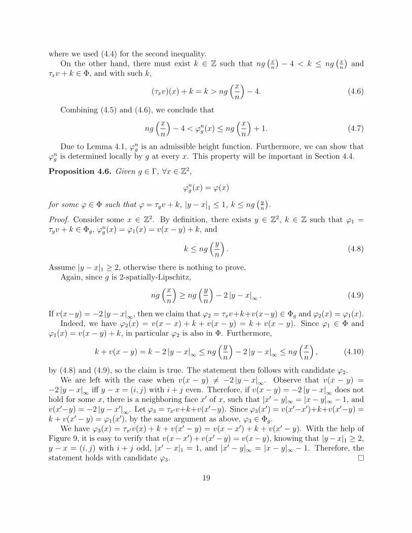4 Smoothing out the height process 1641 Useful properties of the height process 1642 Smoothing out the height process spatially 1743 The space of continuous evolutions 2144 Smoothing out the height process temporally 23

5 Limit points 2851 Precompactness 2852 Characterization of limit points 29

6 Equilibrium measures 3361 Construction of Gibbs measures 3362 Evolution at equilibrium 3663 More on limit points 40

7 Viscosity solution 42

8 Remarks 46

A Proof of Proposition 22 46

B Local interpolations for constructing Sn 47

1 Introduction

The dimer model which consists of the weighted perfect matchings on graphs is a well-studied model in mathematical physics The domino model is the dimer model on a (possiblyinfinite) region of the Z2 lattice Alternatively it can be thought of as tiling a region of thesquare grid exactly by 1times 2 and 2times 1 dominoes For a comprehensive survey on the subjectof dimer models see [16] Necessary knowledge will be reviewed in the paper

The domino shuffling is a discrete-time random dynamics operating on the domino modelintroduced originally by Elkies et al in [6] to compute the generating function of dominotilings of a specific family of graphs called Aztec Diamonds with periodic weights In partic-ular the domino shuffling provides a simple algorithm to generate the uniform measure oftilings of Aztec Diamonds and led to the first rigorous proof of the famous Artic Circle The-orem by Jockusch et al([10]) that describes the asymptotic shape of the central sub-regionof a random tiling

The domino shuffling seemed quite mysterious the way it was presented in [6] initiallyPropp([21]) later gave a much clearer explanation using a procedure called urban renewalor spider move which also allows natural generalizations to different graphs This is theapproach we will take to define the shuffling dynamics in Section 2 As it turns out this alsonaturally converts the shuffling dynamics into a random height process which we shall callthe shuffling height process The height process is a (2 + 1)-dimensional evolution which is

2


ut +H(ux) = 0 (11)


H(ρ1 ρ2) =4

πcosminus1

(1

2cos(πρ2

2

)minus 1

2cos(πρ1

2

))





3





4



2 General setup





5


micro[M isinM] =1

Z

prodeisinM

w(e)

where Z =sum

MisinMprod



22 Height function








6







23 Local moves




7


1 1




1 1

1 1


A =c

ac+ bd B =

d

ac+ bd C =

a

ac+ bdD =

b

ac+ bd (21)




ACAC+BD




8


or








9








1ge hM prime

2still holds af-




10











move








11

3 The main result











12




become 11+a






13




hminus 3


h+ 1



1+a


h+ 1


h+ 1


hminus 3

h+ 1h+ 3 h h+ 3 h

h+ 1




1+aand value 0 with

probability a1+a


14







limnrarrinfin

E sup|x|1leR


∣∣∣∣ = 0 (31)





limnrarrinfin

E sup|x|1leRtleR


∣∣∣∣ = 0 (32)


u(x 0) = g(x)(33)


H(ρ1 ρ2) =4

πcosminus1

(a

1 + acos(πρ2

2

)minus 1

1 + acos(πρ1

2

)) (34)

ut = partupartt




minus

(aπ(cos(πρ12

)+ cos

(πρ22

))(a+ 1)2 minus

(cos(πρ12

)minus a cos

(πρ22

))2

)2



15








h(x tϕ+ 4k ω) = h(x tϕ ω) + 4k (41)









16




= h(y tϕ2 + 4k ω)

= h(y tϕ2 ω) + 4k (by (41))

















17






(yn

)



) Since g


)minus ng

(xn


n

∣∣∣infin


rArr ng(yn

)le ng

(xn





(xn


(xn

)(45)

18


(xn

)minus 4 lt k le ng

(xn

)and



)minus 4 (46)


ng(xn


(xn

)+ 1 (47)



ϕng (x) = ϕ(x)


)



k le ng(yn

) (48)


ng(xn

)ge ng

(yn






(xn

) (410)




19





)



(2i 2j) (2i+ 2 2j) (2i+ 2 2j + 2) (2i 2j + 2)





nN s lt t we define

Sn(s t g ω)(x) =1

nψnsnt(nx)



)∣∣∣∣ lt C0

nforallx isin 1

nZ2 (412)


Sn(s t g ω)(x) = g


20





|g1(x)minus g2(x)| (413)



By definition of Γ


|g1(x)minus g2(x)|



|g2(x)minus g2(0)|

le |g1(0)minus g2(0)|+ 4k (415)










q let



2minusiF1 minus F2i

1 + F1 minus F2i (420)

By (415)



le 2r + 4k

21










Since


we duduce that







leinfinsumi=1



le 2qd(g1 g2)


22






q are required


q

)= C

([0 T ]C

([0 T ] E r

q





D (R1(s t) R2(s t)) (421)






nZ2 belongs to 1


q


Sn(s t g ω) =1

4

int 4

u=0

[Sn


n ω)

+u

n

]du+ g(0)




later in the paper



n+ 4(tminus s)

23






n+ 4(tminus s)



n+ 4(tminus s)


n














n

24


nN



Sn(s t g +mω) =1

4

int 4

u=0

[Sn


n ω)

+u

n

]du+ g(0) +m

= Sn(s t g ω) +m








Let us consider[Sn


n ω)

+u

n+ g2(0)

]minus[Sn


n ω

)+η(u)

n+ g1(0)

]=Sn

(s t f2 minus

u

n ω)minus Sn

(s t f1 minus

η(u)

n ω

)+uminus η(u)

n+ δ0 (422)



n say 4k

nfor some k isin Z


Sn

(s t f2 minus

u

n ω)

= Sn

(s t f2 minus

u

nminus 4k

n ω

)+

4k

n (423)

and (f2 minus

u

nminus 4k

n

)minus(f1 minus

η(u)

n


η(u)minus un

minus 4k

n


nminus 4k

n= 0

25


Sn

(s t f2 minus

u

nminus 4k

n ω

)minus Sn

(s t f1 minus

η(u)

n ω

)ge 0 (424)


LHS of (422) ge 4k

n+uminus η(u)

n+ δ0 = δ ge 0








(s t+

1

n g ω

)∥∥∥∥infinle 10 + 2C0


(s+

1

n t g ω

)∥∥∥∥infinle 10 + 2C0

n


n middot ω

)where (s t) and

(s t+ 1

n

)are both in 1




n+

4

n=

10 + C0

n forallg isin Γ





n t middot ω

)where (s t) and

(s+ 1

n t)

both lie in 1nN2

If s + 1n


n When s + 1




26



nZ2



nZ2






f00 = Sn(s t g ω) f10 = Sn(s+ 1

n t g ω

)

f01 = Sn(s t+ 1

n g ω

) f11 = Sn

(s+ 1

n t+ 1

n g ω

)


Sn

(s+

x

n t+

y

n g ω













n (426)

27


(s t) isin 1nN2

Sn


n ω)

+4k

n= Sn


n+

4k

n ω

) (427)



n+

4k

n ω



n(12 + 2C0 + 2) (428)


Sn(s t g ω) =1

4

int 4

u=0

[Sn


n ω)

+4k

n+

(u

n+ g(0)minus 4k

n

)]du


n(12 + 2C0 + 2 + 4)

5 Limit points

51 Precompactness




28

1 E is closed






lt 2ε+ (10 + 2C0)d1(x y)









S(t1 t3 g) (52)








lim supirarrinfin


29







2q




a(k δ) = 2minuskδ

1 + δ













30















le(10 + 2C0)2

n+

18 + 2C0

n=

38 + 6C0

n (58)




38 + 6C0

n (59)





prime3Sn(tprime1 t



prime3Sn(tprime1 t


le 338 + 6C0

n+ Sn(tprime1 t


prime3Sn(tprime1 t




prime3Sn(tprime1 t





)∣∣∣∣ lt C0

n (511)

31

Let



prime2 g ω)(x)

∣∣∣∣ le 4

n (512)



nZ2 (513)

For all x isin 1nZ2


prime3Sn(tprime1 t





)(x)

∣∣∣∣++




)(x)

∣∣∣∣++


(x)minus 1



) γntprime2ω

)(x)

∣∣∣∣++


(x)minus 1



) γntprime2ω

)(x)

∣∣∣∣le 2C0

n+

4 + C0

n+ 0 =

4 + 3C0

n




prime3Sn(tprime1 t


4 + 3C0 + 2

n=

6 + 3C0

n







32






Sn(s t g ω) =1

4

int 4

u=0

[Sn


n ω)

+u

n

]du+ g(x)


nlt ε so micro(Eε






|g1(y)minus g2(y)|





33




Figure 10


P (nx) =α

π P (ex) =

β

π P (sx) =

γ

π P (wx) =

δ

π (61)

P (nx sx) =1

π2

(αγ +

sinα sin γ

sin β sin δβδ

) (62)

P (ex wx) =1

π2

(βδ +

sin β sin δ

sinα sin γαγ

)= aP (nx sx) (63)

34



(64)


(65)


sin β sin δ





1

1 + acos(πρ1

2

)minus a

1 + acos(πρ2

2

)= cos (β + δ)


β =πρ1

4+

1


4+

1

2cosminus1 (M)


α = minusπρ2

4+

1


πρ2

4+

1

2cosminus1 (minusM)



limnrarrinfin

E sup|x|1leR




(67)

35




P (Mnε ) ge 1minus

sumxisinAε

C1 log2 |bnxc|n2ε2

(68)



sup|x|1leR


rArr sup|x|1leR


ρ

n(69)




lim supnrarrinfin

E sup|x|1leR









36


















1 + aPπρ(nx sx) +

1

1 + aPπρ(ex wx)


=1

πcosminus1

(a

1 + acos(πρ2

2

)minus 1

1 + acos(πρ1

2

))



37


limtrarrinfin

E∣∣∣∣1t h(0 t) +H(ρ)

∣∣∣∣ = 0



limtrarrinfin

P

(∣∣∣∣1t h(0 t) +H(ρ)

∣∣∣∣ gt ε

)= 0 (610)



(minus4

tsumi=1

1Q(xt)(h)





VR(t) = Var

sum|x|1=R


VR(t) = Var

sum|x|1=R

1Q(2xt)(h)


VR(t+ 1) = Var

sum|x|1=R


1Q(2xt)(h)

=VR(t)minus 8 Cov

sum|x|1=R


1Q(2xt)(h)

+ 16VR(t)


radicVR(t)VR(t)



38


inequaility

P

∣∣∣∣∣∣sum|x|1=R



∣∣∣∣∣∣ ge Cε2t2

=C prime

ε3t(612)


P

(sup|x|1=R


1

th(2x 0)

)∣∣∣∣ le ε

10

)gt 1minus δ (613)



1

th(2x t)minus E

(1

th(2x t)

)ge 1

th(0 t) +H(ρ)minus


th(0 t)

∣∣∣∣minus ∣∣∣∣E(1

th(2x t)minus 1

th(0 t)


ε

10minus 2

ε

10=

3

5ε



(3

5εminus 1

10ε

)=εt

2

Therefore

limtrarrinfin

P

(1


)le δ


limtrarrinfin

P

(1


)le δ



limnrarrinfin

E sup|x|1leR


∣∣∣∣ = 0

39


limnrarrinfin



E∣∣∣∣ 1

nth(0 bntc) +H(ρ)

∣∣∣∣ = 0 (614)


limnrarrinfin

E sup|x|1leR



limnrarrinfin

E sup|x|1leR


∣∣∣∣le lim

nrarrinfinE

(sup|x|1leR


∣∣∣∣ 1nh(0 bntc) + tH(ρ)

∣∣∣∣)

=0 + 0 = 0





limnrarr0

E sup|x|1leR


∣∣∣∣ = 0 (616)

for all R gt 0 then

limnrarr0

E sup|x|1leRtleT


∣∣∣∣ = 0 (617)

for all R gt 0


limnrarr0

E sup|x|1leR

1

n


40


sup|x|1leR



1

n


)∣∣+C3

n(619)


sup|x|1leR

1

n



1

n



lim supnrarrinfin

E sup|x|1leRtleT



nrarrinfin

intsup

|x|1leRtleT




intsup

|x|1leR+2T+1

(1

n


C3

n

)dω0

= limnrarrinfin

E sup|x|1leR+2T+1

1

n


nrarr0

C3

n= 0




surely




limirarrinfin

E sup|x|1leR


41

Viewing sup|x|1leR




Emicro sup|x|1leR


E sup|x|1leR


(622)











ut +H(ux) = 0u(x 0) = g(x)

(71)


42


2 u(middot 0) = g


φt(x0 t0) +H(φx(x0 t0)) le 0 (72)


φt(x0 t0) +H(φx(x0 t0)) ge 0 (73)
















43












By Condition (52)












44






φt(x0 t0) +H(φx(x0 t0)) le 0











limnrarrinfin

E sup|x|1leTtleT



= E sup|x|1leTtleT

∣∣∣S(0 t g)(x)minus u(x t)∣∣∣ = 0 (77)


limnrarrinfin

E supxisinR2tleT


nh(bnxc bntcϕng

)∣∣∣∣ = 0 (78)

Also by (47)

limnrarrinfin

supxisinR2


∣∣∣∣ = 0 (79)


45

8 Remarks







46

same By (21)

wTAC + wTBDwTempty

= AC +BD =ac+ bd

(ac+ bd)2=

1

ac+ bd

wTAwTc

=wTBwTd

=wTCwTa

=wTDwTb

=1

ac+ bd

wTemptywTac + wTbd

=1

ac+ bd


wTACwTBD

=AC

BD



probability BDAC+BD








47

Acknowledgement


References














48

















49

1 Introduction

2 General setup


22 Height function

23 Local moves


3 The main result








5 Limit points

51 Precompactness







8 Remarks




ut +H(ux) = 0 (11)


H(ρ1 ρ2) =4

πcosminus1

(1

2cos(πρ2

2

)minus 1

2cos(πρ1

2

))





3





4



2 General setup





5


micro[M isinM] =1

Z

prodeisinM

w(e)

where Z =sum

MisinMprod



22 Height function








6







23 Local moves




7


1 1




1 1

1 1


A =c

ac+ bd B =

d

ac+ bd C =

a

ac+ bdD =

b

ac+ bd (21)




ACAC+BD




8


or








9








1ge hM prime

2still holds af-




10











move








11

3 The main result











12




become 11+a






13




hminus 3


h+ 1



1+a


h+ 1


h+ 1


hminus 3

h+ 1h+ 3 h h+ 3 h

h+ 1




1+aand value 0 with

probability a1+a


14







limnrarrinfin

E sup|x|1leR


∣∣∣∣ = 0 (31)





limnrarrinfin

E sup|x|1leRtleR


∣∣∣∣ = 0 (32)


u(x 0) = g(x)(33)


H(ρ1 ρ2) =4

πcosminus1

(a

1 + acos(πρ2

2

)minus 1

1 + acos(πρ1

2

)) (34)

ut = partupartt




minus

(aπ(cos(πρ12

)+ cos

(πρ22

))(a+ 1)2 minus

(cos(πρ12

)minus a cos

(πρ22

))2

)2



15








h(x tϕ+ 4k ω) = h(x tϕ ω) + 4k (41)









16




= h(y tϕ2 + 4k ω)

= h(y tϕ2 ω) + 4k (by (41))

















17






(yn

)



) Since g


)minus ng

(xn


n

∣∣∣infin


rArr ng(yn

)le ng

(xn





(xn


(xn

)(45)

18


(xn

)minus 4 lt k le ng

(xn

)and



)minus 4 (46)


ng(xn


(xn

)+ 1 (47)



ϕng (x) = ϕ(x)


)



k le ng(yn

) (48)


ng(xn

)ge ng

(yn






(xn

) (410)




19





)



(2i 2j) (2i+ 2 2j) (2i+ 2 2j + 2) (2i 2j + 2)





nN s lt t we define

Sn(s t g ω)(x) =1

nψnsnt(nx)



)∣∣∣∣ lt C0

nforallx isin 1

nZ2 (412)


Sn(s t g ω)(x) = g


20





|g1(x)minus g2(x)| (413)



By definition of Γ


|g1(x)minus g2(x)|



|g2(x)minus g2(0)|

le |g1(0)minus g2(0)|+ 4k (415)










q let



2minusiF1 minus F2i

1 + F1 minus F2i (420)

By (415)



le 2r + 4k

21










Since


we duduce that







leinfinsumi=1



le 2qd(g1 g2)


22






q are required


q

)= C

([0 T ]C

([0 T ] E r

q





D (R1(s t) R2(s t)) (421)






nZ2 belongs to 1


q


Sn(s t g ω) =1

4

int 4

u=0

[Sn


n ω)

+u

n

]du+ g(0)




later in the paper



n+ 4(tminus s)

23






n+ 4(tminus s)



n+ 4(tminus s)


n














n

24


nN



Sn(s t g +mω) =1

4

int 4

u=0

[Sn


n ω)

+u

n

]du+ g(0) +m

= Sn(s t g ω) +m








Let us consider[Sn


n ω)

+u

n+ g2(0)

]minus[Sn


n ω

)+η(u)

n+ g1(0)

]=Sn

(s t f2 minus

u

n ω)minus Sn

(s t f1 minus

η(u)

n ω

)+uminus η(u)

n+ δ0 (422)



n say 4k

nfor some k isin Z


Sn

(s t f2 minus

u

n ω)

= Sn

(s t f2 minus

u

nminus 4k

n ω

)+

4k

n (423)

and (f2 minus

u

nminus 4k

n

)minus(f1 minus

η(u)

n


η(u)minus un

minus 4k

n


nminus 4k

n= 0

25


Sn

(s t f2 minus

u

nminus 4k

n ω

)minus Sn

(s t f1 minus

η(u)

n ω

)ge 0 (424)


LHS of (422) ge 4k

n+uminus η(u)

n+ δ0 = δ ge 0








(s t+

1

n g ω

)∥∥∥∥infinle 10 + 2C0


(s+

1

n t g ω

)∥∥∥∥infinle 10 + 2C0

n


n middot ω

)where (s t) and

(s t+ 1

n

)are both in 1




n+

4

n=

10 + C0

n forallg isin Γ





n t middot ω

)where (s t) and

(s+ 1

n t)

both lie in 1nN2

If s + 1n


n When s + 1




26



nZ2



nZ2






f00 = Sn(s t g ω) f10 = Sn(s+ 1

n t g ω

)

f01 = Sn(s t+ 1

n g ω

) f11 = Sn

(s+ 1

n t+ 1

n g ω

)


Sn

(s+

x

n t+

y

n g ω













n (426)

27


(s t) isin 1nN2

Sn


n ω)

+4k

n= Sn


n+

4k

n ω

) (427)



n+

4k

n ω



n(12 + 2C0 + 2) (428)


Sn(s t g ω) =1

4

int 4

u=0

[Sn


n ω)

+4k

n+

(u

n+ g(0)minus 4k

n

)]du


n(12 + 2C0 + 2 + 4)

5 Limit points

51 Precompactness




28

1 E is closed






lt 2ε+ (10 + 2C0)d1(x y)









S(t1 t3 g) (52)








lim supirarrinfin


29







2q




a(k δ) = 2minuskδ

1 + δ













30















le(10 + 2C0)2

n+

18 + 2C0

n=

38 + 6C0

n (58)




38 + 6C0

n (59)





prime3Sn(tprime1 t



prime3Sn(tprime1 t


le 338 + 6C0

n+ Sn(tprime1 t


prime3Sn(tprime1 t




prime3Sn(tprime1 t





)∣∣∣∣ lt C0

n (511)

31

Let



prime2 g ω)(x)

∣∣∣∣ le 4

n (512)



nZ2 (513)

For all x isin 1nZ2


prime3Sn(tprime1 t





)(x)

∣∣∣∣++




)(x)

∣∣∣∣++


(x)minus 1



) γntprime2ω

)(x)

∣∣∣∣++


(x)minus 1



) γntprime2ω

)(x)

∣∣∣∣le 2C0

n+

4 + C0

n+ 0 =

4 + 3C0

n




prime3Sn(tprime1 t


4 + 3C0 + 2

n=

6 + 3C0

n







32






Sn(s t g ω) =1

4

int 4

u=0

[Sn


n ω)

+u

n

]du+ g(x)


nlt ε so micro(Eε






|g1(y)minus g2(y)|





33




Figure 10


P (nx) =α

π P (ex) =

β

π P (sx) =

γ

π P (wx) =

δ

π (61)

P (nx sx) =1

π2

(αγ +

sinα sin γ

sin β sin δβδ

) (62)

P (ex wx) =1

π2

(βδ +

sin β sin δ

sinα sin γαγ

)= aP (nx sx) (63)

34



(64)


(65)


sin β sin δ





1

1 + acos(πρ1

2

)minus a

1 + acos(πρ2

2

)= cos (β + δ)


β =πρ1

4+

1


4+

1

2cosminus1 (M)


α = minusπρ2

4+

1


πρ2

4+

1

2cosminus1 (minusM)



limnrarrinfin

E sup|x|1leR




(67)

35




P (Mnε ) ge 1minus

sumxisinAε

C1 log2 |bnxc|n2ε2

(68)



sup|x|1leR


rArr sup|x|1leR


ρ

n(69)




lim supnrarrinfin

E sup|x|1leR









36


















1 + aPπρ(nx sx) +

1

1 + aPπρ(ex wx)


=1

πcosminus1

(a

1 + acos(πρ2

2

)minus 1

1 + acos(πρ1

2

))



37


limtrarrinfin

E∣∣∣∣1t h(0 t) +H(ρ)

∣∣∣∣ = 0



limtrarrinfin

P

(∣∣∣∣1t h(0 t) +H(ρ)

∣∣∣∣ gt ε

)= 0 (610)



(minus4

tsumi=1

1Q(xt)(h)





VR(t) = Var

sum|x|1=R


VR(t) = Var

sum|x|1=R

1Q(2xt)(h)


VR(t+ 1) = Var

sum|x|1=R


1Q(2xt)(h)

=VR(t)minus 8 Cov

sum|x|1=R


1Q(2xt)(h)

+ 16VR(t)


radicVR(t)VR(t)



38


inequaility

P

∣∣∣∣∣∣sum|x|1=R



∣∣∣∣∣∣ ge Cε2t2

=C prime

ε3t(612)


P

(sup|x|1=R


1

th(2x 0)

)∣∣∣∣ le ε

10

)gt 1minus δ (613)



1

th(2x t)minus E

(1

th(2x t)

)ge 1

th(0 t) +H(ρ)minus


th(0 t)

∣∣∣∣minus ∣∣∣∣E(1

th(2x t)minus 1

th(0 t)


ε

10minus 2

ε

10=

3

5ε



(3

5εminus 1

10ε

)=εt

2

Therefore

limtrarrinfin

P

(1


)le δ


limtrarrinfin

P

(1


)le δ



limnrarrinfin

E sup|x|1leR


∣∣∣∣ = 0

39


limnrarrinfin



E∣∣∣∣ 1

nth(0 bntc) +H(ρ)

∣∣∣∣ = 0 (614)


limnrarrinfin

E sup|x|1leR



limnrarrinfin

E sup|x|1leR


∣∣∣∣le lim

nrarrinfinE

(sup|x|1leR


∣∣∣∣ 1nh(0 bntc) + tH(ρ)

∣∣∣∣)

=0 + 0 = 0





limnrarr0

E sup|x|1leR


∣∣∣∣ = 0 (616)

for all R gt 0 then

limnrarr0

E sup|x|1leRtleT


∣∣∣∣ = 0 (617)

for all R gt 0


limnrarr0

E sup|x|1leR

1

n


40


sup|x|1leR



1

n


)∣∣+C3

n(619)


sup|x|1leR

1

n



1

n



lim supnrarrinfin

E sup|x|1leRtleT



nrarrinfin

intsup

|x|1leRtleT




intsup

|x|1leR+2T+1

(1

n


C3

n

)dω0

= limnrarrinfin

E sup|x|1leR+2T+1

1

n


nrarr0

C3

n= 0




surely




limirarrinfin

E sup|x|1leR


41

Viewing sup|x|1leR




Emicro sup|x|1leR


E sup|x|1leR


(622)











ut +H(ux) = 0u(x 0) = g(x)

(71)


42


2 u(middot 0) = g


φt(x0 t0) +H(φx(x0 t0)) le 0 (72)


φt(x0 t0) +H(φx(x0 t0)) ge 0 (73)
















43












By Condition (52)












44






φt(x0 t0) +H(φx(x0 t0)) le 0











limnrarrinfin

E sup|x|1leTtleT



= E sup|x|1leTtleT

∣∣∣S(0 t g)(x)minus u(x t)∣∣∣ = 0 (77)


limnrarrinfin

E supxisinR2tleT


nh(bnxc bntcϕng

)∣∣∣∣ = 0 (78)

Also by (47)

limnrarrinfin

supxisinR2


∣∣∣∣ = 0 (79)


45

8 Remarks







46

same By (21)

wTAC + wTBDwTempty

= AC +BD =ac+ bd

(ac+ bd)2=

1

ac+ bd

wTAwTc

=wTBwTd

=wTCwTa

=wTDwTb

=1

ac+ bd

wTemptywTac + wTbd

=1

ac+ bd


wTACwTBD

=AC

BD



probability BDAC+BD








47

Acknowledgement


References














48

















49

1 Introduction

2 General setup


22 Height function

23 Local moves


3 The main result








5 Limit points

51 Precompactness







8 Remarks







4



2 General setup





5


micro[M isinM] =1

Z

prodeisinM

w(e)

where Z =sum

MisinMprod



22 Height function








6







23 Local moves




7


1 1




1 1

1 1


A =c

ac+ bd B =

d

ac+ bd C =

a

ac+ bdD =

b

ac+ bd (21)




ACAC+BD




8


or








9








1ge hM prime

2still holds af-




10











move








11

3 The main result











12




become 11+a






13




hminus 3


h+ 1



1+a


h+ 1


h+ 1


hminus 3

h+ 1h+ 3 h h+ 3 h

h+ 1




1+aand value 0 with

probability a1+a


14







limnrarrinfin

E sup|x|1leR


∣∣∣∣ = 0 (31)





limnrarrinfin

E sup|x|1leRtleR


∣∣∣∣ = 0 (32)


u(x 0) = g(x)(33)


H(ρ1 ρ2) =4

πcosminus1

(a

1 + acos(πρ2

2

)minus 1

1 + acos(πρ1

2

)) (34)

ut = partupartt




minus

(aπ(cos(πρ12

)+ cos

(πρ22

))(a+ 1)2 minus

(cos(πρ12

)minus a cos

(πρ22

))2

)2



15








h(x tϕ+ 4k ω) = h(x tϕ ω) + 4k (41)









16




= h(y tϕ2 + 4k ω)

= h(y tϕ2 ω) + 4k (by (41))

















17






(yn

)



) Since g


)minus ng

(xn


n

∣∣∣infin


rArr ng(yn

)le ng

(xn





(xn


(xn

)(45)

18


(xn

)minus 4 lt k le ng

(xn

)and



)minus 4 (46)


ng(xn


(xn

)+ 1 (47)



ϕng (x) = ϕ(x)


)



k le ng(yn

) (48)


ng(xn

)ge ng

(yn






(xn

) (410)




19





)



(2i 2j) (2i+ 2 2j) (2i+ 2 2j + 2) (2i 2j + 2)





nN s lt t we define

Sn(s t g ω)(x) =1

nψnsnt(nx)



)∣∣∣∣ lt C0

nforallx isin 1

nZ2 (412)


Sn(s t g ω)(x) = g


20





|g1(x)minus g2(x)| (413)



By definition of Γ


|g1(x)minus g2(x)|



|g2(x)minus g2(0)|

le |g1(0)minus g2(0)|+ 4k (415)










q let



2minusiF1 minus F2i

1 + F1 minus F2i (420)

By (415)



le 2r + 4k

21










Since


we duduce that







leinfinsumi=1



le 2qd(g1 g2)


22






q are required


q

)= C

([0 T ]C

([0 T ] E r

q





D (R1(s t) R2(s t)) (421)






nZ2 belongs to 1


q


Sn(s t g ω) =1

4

int 4

u=0

[Sn


n ω)

+u

n

]du+ g(0)




later in the paper



n+ 4(tminus s)

23






n+ 4(tminus s)



n+ 4(tminus s)


n














n

24


nN



Sn(s t g +mω) =1

4

int 4

u=0

[Sn


n ω)

+u

n

]du+ g(0) +m

= Sn(s t g ω) +m








Let us consider[Sn


n ω)

+u

n+ g2(0)

]minus[Sn


n ω

)+η(u)

n+ g1(0)

]=Sn

(s t f2 minus

u

n ω)minus Sn

(s t f1 minus

η(u)

n ω

)+uminus η(u)

n+ δ0 (422)



n say 4k

nfor some k isin Z


Sn

(s t f2 minus

u

n ω)

= Sn

(s t f2 minus

u

nminus 4k

n ω

)+

4k

n (423)

and (f2 minus

u

nminus 4k

n

)minus(f1 minus

η(u)

n


η(u)minus un

minus 4k

n


nminus 4k

n= 0

25


Sn

(s t f2 minus

u

nminus 4k

n ω

)minus Sn

(s t f1 minus

η(u)

n ω

)ge 0 (424)


LHS of (422) ge 4k

n+uminus η(u)

n+ δ0 = δ ge 0








(s t+

1

n g ω

)∥∥∥∥infinle 10 + 2C0


(s+

1

n t g ω

)∥∥∥∥infinle 10 + 2C0

n


n middot ω

)where (s t) and

(s t+ 1

n

)are both in 1




n+

4

n=

10 + C0

n forallg isin Γ





n t middot ω

)where (s t) and

(s+ 1

n t)

both lie in 1nN2

If s + 1n


n When s + 1




26



nZ2



nZ2






f00 = Sn(s t g ω) f10 = Sn(s+ 1

n t g ω

)

f01 = Sn(s t+ 1

n g ω

) f11 = Sn

(s+ 1

n t+ 1

n g ω

)


Sn

(s+

x

n t+

y

n g ω













n (426)

27


(s t) isin 1nN2

Sn


n ω)

+4k

n= Sn


n+

4k

n ω

) (427)



n+

4k

n ω



n(12 + 2C0 + 2) (428)


Sn(s t g ω) =1

4

int 4

u=0

[Sn


n ω)

+4k

n+

(u

n+ g(0)minus 4k

n

)]du


n(12 + 2C0 + 2 + 4)

5 Limit points

51 Precompactness




28

1 E is closed






lt 2ε+ (10 + 2C0)d1(x y)









S(t1 t3 g) (52)








lim supirarrinfin


29







2q




a(k δ) = 2minuskδ

1 + δ













30















le(10 + 2C0)2

n+

18 + 2C0

n=

38 + 6C0

n (58)




38 + 6C0

n (59)





prime3Sn(tprime1 t



prime3Sn(tprime1 t


le 338 + 6C0

n+ Sn(tprime1 t


prime3Sn(tprime1 t




prime3Sn(tprime1 t





)∣∣∣∣ lt C0

n (511)

31

Let



prime2 g ω)(x)

∣∣∣∣ le 4

n (512)



nZ2 (513)

For all x isin 1nZ2


prime3Sn(tprime1 t





)(x)

∣∣∣∣++




)(x)

∣∣∣∣++


(x)minus 1



) γntprime2ω

)(x)

∣∣∣∣++


(x)minus 1



) γntprime2ω

)(x)

∣∣∣∣le 2C0

n+

4 + C0

n+ 0 =

4 + 3C0

n




prime3Sn(tprime1 t


4 + 3C0 + 2

n=

6 + 3C0

n







32






Sn(s t g ω) =1

4

int 4

u=0

[Sn


n ω)

+u

n

]du+ g(x)


nlt ε so micro(Eε






|g1(y)minus g2(y)|





33




Figure 10


P (nx) =α

π P (ex) =

β

π P (sx) =

γ

π P (wx) =

δ

π (61)

P (nx sx) =1

π2

(αγ +

sinα sin γ

sin β sin δβδ

) (62)

P (ex wx) =1

π2

(βδ +

sin β sin δ

sinα sin γαγ

)= aP (nx sx) (63)

34



(64)


(65)


sin β sin δ





1

1 + acos(πρ1

2

)minus a

1 + acos(πρ2

2

)= cos (β + δ)


β =πρ1

4+

1


4+

1

2cosminus1 (M)


α = minusπρ2

4+

1


πρ2

4+

1

2cosminus1 (minusM)



limnrarrinfin

E sup|x|1leR




(67)

35




P (Mnε ) ge 1minus

sumxisinAε

C1 log2 |bnxc|n2ε2

(68)



sup|x|1leR


rArr sup|x|1leR


ρ

n(69)




lim supnrarrinfin

E sup|x|1leR









36


















1 + aPπρ(nx sx) +

1

1 + aPπρ(ex wx)


=1

πcosminus1

(a

1 + acos(πρ2

2

)minus 1

1 + acos(πρ1

2

))



37


limtrarrinfin

E∣∣∣∣1t h(0 t) +H(ρ)

∣∣∣∣ = 0



limtrarrinfin

P

(∣∣∣∣1t h(0 t) +H(ρ)

∣∣∣∣ gt ε

)= 0 (610)



(minus4

tsumi=1

1Q(xt)(h)





VR(t) = Var

sum|x|1=R


VR(t) = Var

sum|x|1=R

1Q(2xt)(h)


VR(t+ 1) = Var

sum|x|1=R


1Q(2xt)(h)

=VR(t)minus 8 Cov

sum|x|1=R


1Q(2xt)(h)

+ 16VR(t)


radicVR(t)VR(t)



38


inequaility

P

∣∣∣∣∣∣sum|x|1=R



∣∣∣∣∣∣ ge Cε2t2

=C prime

ε3t(612)


P

(sup|x|1=R


1

th(2x 0)

)∣∣∣∣ le ε

10

)gt 1minus δ (613)



1

th(2x t)minus E

(1

th(2x t)

)ge 1

th(0 t) +H(ρ)minus


th(0 t)

∣∣∣∣minus ∣∣∣∣E(1

th(2x t)minus 1

th(0 t)


ε

10minus 2

ε

10=

3

5ε



(3

5εminus 1

10ε

)=εt

2

Therefore

limtrarrinfin

P

(1


)le δ


limtrarrinfin

P

(1


)le δ



limnrarrinfin

E sup|x|1leR


∣∣∣∣ = 0

39


limnrarrinfin



E∣∣∣∣ 1

nth(0 bntc) +H(ρ)

∣∣∣∣ = 0 (614)


limnrarrinfin

E sup|x|1leR



limnrarrinfin

E sup|x|1leR


∣∣∣∣le lim

nrarrinfinE

(sup|x|1leR


∣∣∣∣ 1nh(0 bntc) + tH(ρ)

∣∣∣∣)

=0 + 0 = 0





limnrarr0

E sup|x|1leR


∣∣∣∣ = 0 (616)

for all R gt 0 then

limnrarr0

E sup|x|1leRtleT


∣∣∣∣ = 0 (617)

for all R gt 0


limnrarr0

E sup|x|1leR

1

n


40


sup|x|1leR



1

n


)∣∣+C3

n(619)


sup|x|1leR

1

n



1

n



lim supnrarrinfin

E sup|x|1leRtleT



nrarrinfin

intsup

|x|1leRtleT




intsup

|x|1leR+2T+1

(1

n


C3

n

)dω0

= limnrarrinfin

E sup|x|1leR+2T+1

1

n


nrarr0

C3

n= 0




surely




limirarrinfin

E sup|x|1leR


41

Viewing sup|x|1leR




Emicro sup|x|1leR


E sup|x|1leR


(622)











ut +H(ux) = 0u(x 0) = g(x)

(71)


42


2 u(middot 0) = g


φt(x0 t0) +H(φx(x0 t0)) le 0 (72)


φt(x0 t0) +H(φx(x0 t0)) ge 0 (73)
















43












By Condition (52)












44






φt(x0 t0) +H(φx(x0 t0)) le 0











limnrarrinfin

E sup|x|1leTtleT



= E sup|x|1leTtleT

∣∣∣S(0 t g)(x)minus u(x t)∣∣∣ = 0 (77)


limnrarrinfin

E supxisinR2tleT


nh(bnxc bntcϕng

)∣∣∣∣ = 0 (78)

Also by (47)

limnrarrinfin

supxisinR2


∣∣∣∣ = 0 (79)


45

8 Remarks







46

same By (21)

wTAC + wTBDwTempty

= AC +BD =ac+ bd

(ac+ bd)2=

1

ac+ bd

wTAwTc

=wTBwTd

=wTCwTa

=wTDwTb

=1

ac+ bd

wTemptywTac + wTbd

=1

ac+ bd


wTACwTBD

=AC

BD



probability BDAC+BD








47

Acknowledgement


References














48

















49

1 Introduction

2 General setup


22 Height function

23 Local moves


3 The main result








5 Limit points

51 Precompactness







8 Remarks





2 General setup





5


micro[M isinM] =1

Z

prodeisinM

w(e)

where Z =sum

MisinMprod



22 Height function








6







23 Local moves




7


1 1




1 1

1 1


A =c

ac+ bd B =

d

ac+ bd C =

a

ac+ bdD =

b

ac+ bd (21)




ACAC+BD




8


or








9








1ge hM prime

2still holds af-




10











move








11

3 The main result











12




become 11+a






13




hminus 3


h+ 1



1+a


h+ 1


h+ 1


hminus 3

h+ 1h+ 3 h h+ 3 h

h+ 1




1+aand value 0 with

probability a1+a


14







limnrarrinfin

E sup|x|1leR


∣∣∣∣ = 0 (31)





limnrarrinfin

E sup|x|1leRtleR


∣∣∣∣ = 0 (32)


u(x 0) = g(x)(33)


H(ρ1 ρ2) =4

πcosminus1

(a

1 + acos(πρ2

2

)minus 1

1 + acos(πρ1

2

)) (34)

ut = partupartt




minus

(aπ(cos(πρ12

)+ cos

(πρ22

))(a+ 1)2 minus

(cos(πρ12

)minus a cos

(πρ22

))2

)2



15








h(x tϕ+ 4k ω) = h(x tϕ ω) + 4k (41)









16




= h(y tϕ2 + 4k ω)

= h(y tϕ2 ω) + 4k (by (41))

















17






(yn

)



) Since g


)minus ng

(xn


n

∣∣∣infin


rArr ng(yn

)le ng

(xn





(xn


(xn

)(45)

18


(xn

)minus 4 lt k le ng

(xn

)and



)minus 4 (46)


ng(xn


(xn

)+ 1 (47)



ϕng (x) = ϕ(x)


)



k le ng(yn

) (48)


ng(xn

)ge ng

(yn






(xn

) (410)




19





)



(2i 2j) (2i+ 2 2j) (2i+ 2 2j + 2) (2i 2j + 2)





nN s lt t we define

Sn(s t g ω)(x) =1

nψnsnt(nx)



)∣∣∣∣ lt C0

nforallx isin 1

nZ2 (412)


Sn(s t g ω)(x) = g


20





|g1(x)minus g2(x)| (413)



By definition of Γ


|g1(x)minus g2(x)|



|g2(x)minus g2(0)|

le |g1(0)minus g2(0)|+ 4k (415)










q let



2minusiF1 minus F2i

1 + F1 minus F2i (420)

By (415)



le 2r + 4k

21










Since


we duduce that







leinfinsumi=1



le 2qd(g1 g2)


22






q are required


q

)= C

([0 T ]C

([0 T ] E r

q





D (R1(s t) R2(s t)) (421)






nZ2 belongs to 1


q


Sn(s t g ω) =1

4

int 4

u=0

[Sn


n ω)

+u

n

]du+ g(0)




later in the paper



n+ 4(tminus s)

23






n+ 4(tminus s)



n+ 4(tminus s)


n














n

24


nN



Sn(s t g +mω) =1

4

int 4

u=0

[Sn


n ω)

+u

n

]du+ g(0) +m

= Sn(s t g ω) +m








Let us consider[Sn


n ω)

+u

n+ g2(0)

]minus[Sn


n ω

)+η(u)

n+ g1(0)

]=Sn

(s t f2 minus

u

n ω)minus Sn

(s t f1 minus

η(u)

n ω

)+uminus η(u)

n+ δ0 (422)



n say 4k

nfor some k isin Z


Sn

(s t f2 minus

u

n ω)

= Sn

(s t f2 minus

u

nminus 4k

n ω

)+

4k

n (423)

and (f2 minus

u

nminus 4k

n

)minus(f1 minus

η(u)

n


η(u)minus un

minus 4k

n


nminus 4k

n= 0

25


Sn

(s t f2 minus

u

nminus 4k

n ω

)minus Sn

(s t f1 minus

η(u)

n ω

)ge 0 (424)


LHS of (422) ge 4k

n+uminus η(u)

n+ δ0 = δ ge 0








(s t+

1

n g ω

)∥∥∥∥infinle 10 + 2C0


(s+

1

n t g ω

)∥∥∥∥infinle 10 + 2C0

n


n middot ω

)where (s t) and

(s t+ 1

n

)are both in 1




n+

4

n=

10 + C0

n forallg isin Γ





n t middot ω

)where (s t) and

(s+ 1

n t)

both lie in 1nN2

If s + 1n


n When s + 1




26



nZ2



nZ2






f00 = Sn(s t g ω) f10 = Sn(s+ 1

n t g ω

)

f01 = Sn(s t+ 1

n g ω

) f11 = Sn

(s+ 1

n t+ 1

n g ω

)


Sn

(s+

x

n t+

y

n g ω













n (426)

27


(s t) isin 1nN2

Sn


n ω)

+4k

n= Sn


n+

4k

n ω

) (427)



n+

4k

n ω



n(12 + 2C0 + 2) (428)


Sn(s t g ω) =1

4

int 4

u=0

[Sn


n ω)

+4k

n+

(u

n+ g(0)minus 4k

n

)]du


n(12 + 2C0 + 2 + 4)

5 Limit points

51 Precompactness




28

1 E is closed






lt 2ε+ (10 + 2C0)d1(x y)









S(t1 t3 g) (52)








lim supirarrinfin


29







2q




a(k δ) = 2minuskδ

1 + δ













30















le(10 + 2C0)2

n+

18 + 2C0

n=

38 + 6C0

n (58)




38 + 6C0

n (59)





prime3Sn(tprime1 t



prime3Sn(tprime1 t


le 338 + 6C0

n+ Sn(tprime1 t


prime3Sn(tprime1 t




prime3Sn(tprime1 t





)∣∣∣∣ lt C0

n (511)

31

Let



prime2 g ω)(x)

∣∣∣∣ le 4

n (512)



nZ2 (513)

For all x isin 1nZ2


prime3Sn(tprime1 t





)(x)

∣∣∣∣++




)(x)

∣∣∣∣++


(x)minus 1



) γntprime2ω

)(x)

∣∣∣∣++


(x)minus 1



) γntprime2ω

)(x)

∣∣∣∣le 2C0

n+

4 + C0

n+ 0 =

4 + 3C0

n




prime3Sn(tprime1 t


4 + 3C0 + 2

n=

6 + 3C0

n







32






Sn(s t g ω) =1

4

int 4

u=0

[Sn


n ω)

+u

n

]du+ g(x)


nlt ε so micro(Eε






|g1(y)minus g2(y)|





33




Figure 10


P (nx) =α

π P (ex) =

β

π P (sx) =

γ

π P (wx) =

δ

π (61)

P (nx sx) =1

π2

(αγ +

sinα sin γ

sin β sin δβδ

) (62)

P (ex wx) =1

π2

(βδ +

sin β sin δ

sinα sin γαγ

)= aP (nx sx) (63)

34



(64)


(65)


sin β sin δ





1

1 + acos(πρ1

2

)minus a

1 + acos(πρ2

2

)= cos (β + δ)


β =πρ1

4+

1


4+

1

2cosminus1 (M)


α = minusπρ2

4+

1


πρ2

4+

1

2cosminus1 (minusM)



limnrarrinfin

E sup|x|1leR




(67)

35




P (Mnε ) ge 1minus

sumxisinAε

C1 log2 |bnxc|n2ε2

(68)



sup|x|1leR


rArr sup|x|1leR


ρ

n(69)




lim supnrarrinfin

E sup|x|1leR









36


















1 + aPπρ(nx sx) +

1

1 + aPπρ(ex wx)


=1

πcosminus1

(a

1 + acos(πρ2

2

)minus 1

1 + acos(πρ1

2

))



37


limtrarrinfin

E∣∣∣∣1t h(0 t) +H(ρ)

∣∣∣∣ = 0



limtrarrinfin

P

(∣∣∣∣1t h(0 t) +H(ρ)

∣∣∣∣ gt ε

)= 0 (610)



(minus4

tsumi=1

1Q(xt)(h)





VR(t) = Var

sum|x|1=R


VR(t) = Var

sum|x|1=R

1Q(2xt)(h)


VR(t+ 1) = Var

sum|x|1=R


1Q(2xt)(h)

=VR(t)minus 8 Cov

sum|x|1=R


1Q(2xt)(h)

+ 16VR(t)


radicVR(t)VR(t)



38


inequaility

P

∣∣∣∣∣∣sum|x|1=R



∣∣∣∣∣∣ ge Cε2t2

=C prime

ε3t(612)


P

(sup|x|1=R


1

th(2x 0)

)∣∣∣∣ le ε

10

)gt 1minus δ (613)



1

th(2x t)minus E

(1

th(2x t)

)ge 1

th(0 t) +H(ρ)minus


th(0 t)

∣∣∣∣minus ∣∣∣∣E(1

th(2x t)minus 1

th(0 t)


ε

10minus 2

ε

10=

3

5ε



(3

5εminus 1

10ε

)=εt

2

Therefore

limtrarrinfin

P

(1


)le δ


limtrarrinfin

P

(1


)le δ



limnrarrinfin

E sup|x|1leR


∣∣∣∣ = 0

39


limnrarrinfin



E∣∣∣∣ 1

nth(0 bntc) +H(ρ)

∣∣∣∣ = 0 (614)


limnrarrinfin

E sup|x|1leR



limnrarrinfin

E sup|x|1leR


∣∣∣∣le lim

nrarrinfinE

(sup|x|1leR


∣∣∣∣ 1nh(0 bntc) + tH(ρ)

∣∣∣∣)

=0 + 0 = 0





limnrarr0

E sup|x|1leR


∣∣∣∣ = 0 (616)

for all R gt 0 then

limnrarr0

E sup|x|1leRtleT


∣∣∣∣ = 0 (617)

for all R gt 0


limnrarr0

E sup|x|1leR

1

n


40


sup|x|1leR



1

n


)∣∣+C3

n(619)


sup|x|1leR

1

n



1

n



lim supnrarrinfin

E sup|x|1leRtleT



nrarrinfin

intsup

|x|1leRtleT




intsup

|x|1leR+2T+1

(1

n


C3

n

)dω0

= limnrarrinfin

E sup|x|1leR+2T+1

1

n


nrarr0

C3

n= 0




surely




limirarrinfin

E sup|x|1leR


41

Viewing sup|x|1leR




Emicro sup|x|1leR


E sup|x|1leR


(622)











ut +H(ux) = 0u(x 0) = g(x)

(71)


42


2 u(middot 0) = g


φt(x0 t0) +H(φx(x0 t0)) le 0 (72)


φt(x0 t0) +H(φx(x0 t0)) ge 0 (73)
















43












By Condition (52)












44






φt(x0 t0) +H(φx(x0 t0)) le 0











limnrarrinfin

E sup|x|1leTtleT



= E sup|x|1leTtleT

∣∣∣S(0 t g)(x)minus u(x t)∣∣∣ = 0 (77)


limnrarrinfin

E supxisinR2tleT


nh(bnxc bntcϕng

)∣∣∣∣ = 0 (78)

Also by (47)

limnrarrinfin

supxisinR2


∣∣∣∣ = 0 (79)


45

8 Remarks







46

same By (21)

wTAC + wTBDwTempty

= AC +BD =ac+ bd

(ac+ bd)2=

1

ac+ bd

wTAwTc

=wTBwTd

=wTCwTa

=wTDwTb

=1

ac+ bd

wTemptywTac + wTbd

=1

ac+ bd


wTACwTBD

=AC

BD



probability BDAC+BD








47

Acknowledgement


References














48

















49

1 Introduction

2 General setup


22 Height function

23 Local moves


3 The main result








5 Limit points

51 Precompactness







8 Remarks




micro[M isinM] =1

Z

prodeisinM

w(e)

where Z =sum

MisinMprod



22 Height function








6







23 Local moves




7


1 1




1 1

1 1


A =c

ac+ bd B =

d

ac+ bd C =

a

ac+ bdD =

b

ac+ bd (21)




ACAC+BD




8


or








9








1ge hM prime

2still holds af-




10











move








11

3 The main result











12




become 11+a






13




hminus 3


h+ 1



1+a


h+ 1


h+ 1


hminus 3

h+ 1h+ 3 h h+ 3 h

h+ 1




1+aand value 0 with

probability a1+a


14







limnrarrinfin

E sup|x|1leR


∣∣∣∣ = 0 (31)





limnrarrinfin

E sup|x|1leRtleR


∣∣∣∣ = 0 (32)


u(x 0) = g(x)(33)


H(ρ1 ρ2) =4

πcosminus1

(a

1 + acos(πρ2

2

)minus 1

1 + acos(πρ1

2

)) (34)

ut = partupartt




minus

(aπ(cos(πρ12

)+ cos

(πρ22

))(a+ 1)2 minus

(cos(πρ12

)minus a cos

(πρ22

))2

)2



15








h(x tϕ+ 4k ω) = h(x tϕ ω) + 4k (41)









16




= h(y tϕ2 + 4k ω)

= h(y tϕ2 ω) + 4k (by (41))

















17






(yn

)



) Since g


)minus ng

(xn


n

∣∣∣infin


rArr ng(yn

)le ng

(xn





(xn


(xn

)(45)

18


(xn

)minus 4 lt k le ng

(xn

)and



)minus 4 (46)


ng(xn


(xn

)+ 1 (47)



ϕng (x) = ϕ(x)


)



k le ng(yn

) (48)


ng(xn

)ge ng

(yn






(xn

) (410)




19





)



(2i 2j) (2i+ 2 2j) (2i+ 2 2j + 2) (2i 2j + 2)





nN s lt t we define

Sn(s t g ω)(x) =1

nψnsnt(nx)



)∣∣∣∣ lt C0

nforallx isin 1

nZ2 (412)


Sn(s t g ω)(x) = g


20





|g1(x)minus g2(x)| (413)



By definition of Γ


|g1(x)minus g2(x)|



|g2(x)minus g2(0)|

le |g1(0)minus g2(0)|+ 4k (415)










q let



2minusiF1 minus F2i

1 + F1 minus F2i (420)

By (415)



le 2r + 4k

21










Since


we duduce that







leinfinsumi=1



le 2qd(g1 g2)


22






q are required


q

)= C

([0 T ]C

([0 T ] E r

q





D (R1(s t) R2(s t)) (421)






nZ2 belongs to 1


q


Sn(s t g ω) =1

4

int 4

u=0

[Sn


n ω)

+u

n

]du+ g(0)




later in the paper



n+ 4(tminus s)

23






n+ 4(tminus s)



n+ 4(tminus s)


n














n

24


nN



Sn(s t g +mω) =1

4

int 4

u=0

[Sn


n ω)

+u

n

]du+ g(0) +m

= Sn(s t g ω) +m








Let us consider[Sn


n ω)

+u

n+ g2(0)

]minus[Sn


n ω

)+η(u)

n+ g1(0)

]=Sn

(s t f2 minus

u

n ω)minus Sn

(s t f1 minus

η(u)

n ω

)+uminus η(u)

n+ δ0 (422)



n say 4k

nfor some k isin Z


Sn

(s t f2 minus

u

n ω)

= Sn

(s t f2 minus

u

nminus 4k

n ω

)+

4k

n (423)

and (f2 minus

u

nminus 4k

n

)minus(f1 minus

η(u)

n


η(u)minus un

minus 4k

n


nminus 4k

n= 0

25


Sn

(s t f2 minus

u

nminus 4k

n ω

)minus Sn

(s t f1 minus

η(u)

n ω

)ge 0 (424)


LHS of (422) ge 4k

n+uminus η(u)

n+ δ0 = δ ge 0








(s t+

1

n g ω

)∥∥∥∥infinle 10 + 2C0


(s+

1

n t g ω

)∥∥∥∥infinle 10 + 2C0

n


n middot ω

)where (s t) and

(s t+ 1

n

)are both in 1




n+

4

n=

10 + C0

n forallg isin Γ





n t middot ω

)where (s t) and

(s+ 1

n t)

both lie in 1nN2

If s + 1n


n When s + 1




26



nZ2



nZ2






f00 = Sn(s t g ω) f10 = Sn(s+ 1

n t g ω

)

f01 = Sn(s t+ 1

n g ω

) f11 = Sn

(s+ 1

n t+ 1

n g ω

)


Sn

(s+

x

n t+

y

n g ω













n (426)

27


(s t) isin 1nN2

Sn


n ω)

+4k

n= Sn


n+

4k

n ω

) (427)



n+

4k

n ω



n(12 + 2C0 + 2) (428)


Sn(s t g ω) =1

4

int 4

u=0

[Sn


n ω)

+4k

n+

(u

n+ g(0)minus 4k

n

)]du


n(12 + 2C0 + 2 + 4)

5 Limit points

51 Precompactness




28

1 E is closed






lt 2ε+ (10 + 2C0)d1(x y)









S(t1 t3 g) (52)








lim supirarrinfin


29







2q




a(k δ) = 2minuskδ

1 + δ













30















le(10 + 2C0)2

n+

18 + 2C0

n=

38 + 6C0

n (58)




38 + 6C0

n (59)





prime3Sn(tprime1 t



prime3Sn(tprime1 t


le 338 + 6C0

n+ Sn(tprime1 t


prime3Sn(tprime1 t




prime3Sn(tprime1 t





)∣∣∣∣ lt C0

n (511)

31

Let



prime2 g ω)(x)

∣∣∣∣ le 4

n (512)



nZ2 (513)

For all x isin 1nZ2


prime3Sn(tprime1 t





)(x)

∣∣∣∣++




)(x)

∣∣∣∣++


(x)minus 1



) γntprime2ω

)(x)

∣∣∣∣++


(x)minus 1



) γntprime2ω

)(x)

∣∣∣∣le 2C0

n+

4 + C0

n+ 0 =

4 + 3C0

n




prime3Sn(tprime1 t


4 + 3C0 + 2

n=

6 + 3C0

n







32






Sn(s t g ω) =1

4

int 4

u=0

[Sn


n ω)

+u

n

]du+ g(x)


nlt ε so micro(Eε






|g1(y)minus g2(y)|





33




Figure 10


P (nx) =α

π P (ex) =

β

π P (sx) =

γ

π P (wx) =

δ

π (61)

P (nx sx) =1

π2

(αγ +

sinα sin γ

sin β sin δβδ

) (62)

P (ex wx) =1

π2

(βδ +

sin β sin δ

sinα sin γαγ

)= aP (nx sx) (63)

34



(64)


(65)


sin β sin δ





1

1 + acos(πρ1

2

)minus a

1 + acos(πρ2

2

)= cos (β + δ)


β =πρ1

4+

1


4+

1

2cosminus1 (M)


α = minusπρ2

4+

1


πρ2

4+

1

2cosminus1 (minusM)



limnrarrinfin

E sup|x|1leR




(67)

35




P (Mnε ) ge 1minus

sumxisinAε

C1 log2 |bnxc|n2ε2

(68)



sup|x|1leR


rArr sup|x|1leR


ρ

n(69)




lim supnrarrinfin

E sup|x|1leR









36


















1 + aPπρ(nx sx) +

1

1 + aPπρ(ex wx)


=1

πcosminus1

(a

1 + acos(πρ2

2

)minus 1

1 + acos(πρ1

2

))



37


limtrarrinfin

E∣∣∣∣1t h(0 t) +H(ρ)

∣∣∣∣ = 0



limtrarrinfin

P

(∣∣∣∣1t h(0 t) +H(ρ)

∣∣∣∣ gt ε

)= 0 (610)



(minus4

tsumi=1

1Q(xt)(h)





VR(t) = Var

sum|x|1=R


VR(t) = Var

sum|x|1=R

1Q(2xt)(h)


VR(t+ 1) = Var

sum|x|1=R


1Q(2xt)(h)

=VR(t)minus 8 Cov

sum|x|1=R


1Q(2xt)(h)

+ 16VR(t)


radicVR(t)VR(t)



38


inequaility

P

∣∣∣∣∣∣sum|x|1=R



∣∣∣∣∣∣ ge Cε2t2

=C prime

ε3t(612)


P

(sup|x|1=R


1

th(2x 0)

)∣∣∣∣ le ε

10

)gt 1minus δ (613)



1

th(2x t)minus E

(1

th(2x t)

)ge 1

th(0 t) +H(ρ)minus


th(0 t)

∣∣∣∣minus ∣∣∣∣E(1

th(2x t)minus 1

th(0 t)


ε

10minus 2

ε

10=

3

5ε



(3

5εminus 1

10ε

)=εt

2

Therefore

limtrarrinfin

P

(1


)le δ


limtrarrinfin

P

(1


)le δ



limnrarrinfin

E sup|x|1leR


∣∣∣∣ = 0

39


limnrarrinfin



E∣∣∣∣ 1

nth(0 bntc) +H(ρ)

∣∣∣∣ = 0 (614)


limnrarrinfin

E sup|x|1leR



limnrarrinfin

E sup|x|1leR


∣∣∣∣le lim

nrarrinfinE

(sup|x|1leR


∣∣∣∣ 1nh(0 bntc) + tH(ρ)

∣∣∣∣)

=0 + 0 = 0





limnrarr0

E sup|x|1leR


∣∣∣∣ = 0 (616)

for all R gt 0 then

limnrarr0

E sup|x|1leRtleT


∣∣∣∣ = 0 (617)

for all R gt 0


limnrarr0

E sup|x|1leR

1

n


40


sup|x|1leR



1

n


)∣∣+C3

n(619)


sup|x|1leR

1

n



1

n



lim supnrarrinfin

E sup|x|1leRtleT



nrarrinfin

intsup

|x|1leRtleT




intsup

|x|1leR+2T+1

(1

n


C3

n

)dω0

= limnrarrinfin

E sup|x|1leR+2T+1

1

n


nrarr0

C3

n= 0




surely




limirarrinfin

E sup|x|1leR


41

Viewing sup|x|1leR




Emicro sup|x|1leR


E sup|x|1leR


(622)











ut +H(ux) = 0u(x 0) = g(x)

(71)


42


2 u(middot 0) = g


φt(x0 t0) +H(φx(x0 t0)) le 0 (72)


φt(x0 t0) +H(φx(x0 t0)) ge 0 (73)
















43












By Condition (52)












44






φt(x0 t0) +H(φx(x0 t0)) le 0











limnrarrinfin

E sup|x|1leTtleT



= E sup|x|1leTtleT

∣∣∣S(0 t g)(x)minus u(x t)∣∣∣ = 0 (77)


limnrarrinfin

E supxisinR2tleT


nh(bnxc bntcϕng

)∣∣∣∣ = 0 (78)

Also by (47)

limnrarrinfin

supxisinR2


∣∣∣∣ = 0 (79)


45

8 Remarks







46

same By (21)

wTAC + wTBDwTempty

= AC +BD =ac+ bd

(ac+ bd)2=

1

ac+ bd

wTAwTc

=wTBwTd

=wTCwTa

=wTDwTb

=1

ac+ bd

wTemptywTac + wTbd

=1

ac+ bd


wTACwTBD

=AC

BD



probability BDAC+BD








47

Acknowledgement


References














48

















49

1 Introduction

2 General setup


22 Height function

23 Local moves


3 The main result








5 Limit points

51 Precompactness







8 Remarks









23 Local moves




7


1 1




1 1

1 1


A =c

ac+ bd B =

d

ac+ bd C =

a

ac+ bdD =

b

ac+ bd (21)




ACAC+BD




8


or








9








1ge hM prime

2still holds af-




10











move








11

3 The main result











12




become 11+a






13




hminus 3


h+ 1



1+a


h+ 1


h+ 1


hminus 3

h+ 1h+ 3 h h+ 3 h

h+ 1




1+aand value 0 with

probability a1+a


14







limnrarrinfin

E sup|x|1leR


∣∣∣∣ = 0 (31)





limnrarrinfin

E sup|x|1leRtleR


∣∣∣∣ = 0 (32)


u(x 0) = g(x)(33)


H(ρ1 ρ2) =4

πcosminus1

(a

1 + acos(πρ2

2

)minus 1

1 + acos(πρ1

2

)) (34)

ut = partupartt




minus

(aπ(cos(πρ12

)+ cos

(πρ22

))(a+ 1)2 minus

(cos(πρ12

)minus a cos

(πρ22

))2

)2



15








h(x tϕ+ 4k ω) = h(x tϕ ω) + 4k (41)









16




= h(y tϕ2 + 4k ω)

= h(y tϕ2 ω) + 4k (by (41))

















17






(yn

)



) Since g


)minus ng

(xn


n

∣∣∣infin


rArr ng(yn

)le ng

(xn





(xn


(xn

)(45)

18


(xn

)minus 4 lt k le ng

(xn

)and



)minus 4 (46)


ng(xn


(xn

)+ 1 (47)



ϕng (x) = ϕ(x)


)



k le ng(yn

) (48)


ng(xn

)ge ng

(yn






(xn

) (410)




19





)



(2i 2j) (2i+ 2 2j) (2i+ 2 2j + 2) (2i 2j + 2)





nN s lt t we define

Sn(s t g ω)(x) =1

nψnsnt(nx)



)∣∣∣∣ lt C0

nforallx isin 1

nZ2 (412)


Sn(s t g ω)(x) = g


20





|g1(x)minus g2(x)| (413)



By definition of Γ


|g1(x)minus g2(x)|



|g2(x)minus g2(0)|

le |g1(0)minus g2(0)|+ 4k (415)










q let



2minusiF1 minus F2i

1 + F1 minus F2i (420)

By (415)



le 2r + 4k

21










Since


we duduce that







leinfinsumi=1



le 2qd(g1 g2)


22






q are required


q

)= C

([0 T ]C

([0 T ] E r

q





D (R1(s t) R2(s t)) (421)






nZ2 belongs to 1


q


Sn(s t g ω) =1

4

int 4

u=0

[Sn


n ω)

+u

n

]du+ g(0)




later in the paper



n+ 4(tminus s)

23






n+ 4(tminus s)



n+ 4(tminus s)


n














n

24


nN



Sn(s t g +mω) =1

4

int 4

u=0

[Sn


n ω)

+u

n

]du+ g(0) +m

= Sn(s t g ω) +m








Let us consider[Sn


n ω)

+u

n+ g2(0)

]minus[Sn


n ω

)+η(u)

n+ g1(0)

]=Sn

(s t f2 minus

u

n ω)minus Sn

(s t f1 minus

η(u)

n ω

)+uminus η(u)

n+ δ0 (422)



n say 4k

nfor some k isin Z


Sn

(s t f2 minus

u

n ω)

= Sn

(s t f2 minus

u

nminus 4k

n ω

)+

4k

n (423)

and (f2 minus

u

nminus 4k

n

)minus(f1 minus

η(u)

n


η(u)minus un

minus 4k

n


nminus 4k

n= 0

25


Sn

(s t f2 minus

u

nminus 4k

n ω

)minus Sn

(s t f1 minus

η(u)

n ω

)ge 0 (424)


LHS of (422) ge 4k

n+uminus η(u)

n+ δ0 = δ ge 0








(s t+

1

n g ω

)∥∥∥∥infinle 10 + 2C0


(s+

1

n t g ω

)∥∥∥∥infinle 10 + 2C0

n


n middot ω

)where (s t) and

(s t+ 1

n

)are both in 1




n+

4

n=

10 + C0

n forallg isin Γ





n t middot ω

)where (s t) and

(s+ 1

n t)

both lie in 1nN2

If s + 1n


n When s + 1




26



nZ2



nZ2






f00 = Sn(s t g ω) f10 = Sn(s+ 1

n t g ω

)

f01 = Sn(s t+ 1

n g ω

) f11 = Sn

(s+ 1

n t+ 1

n g ω

)


Sn

(s+

x

n t+

y

n g ω













n (426)

27


(s t) isin 1nN2

Sn


n ω)

+4k

n= Sn


n+

4k

n ω

) (427)



n+

4k

n ω



n(12 + 2C0 + 2) (428)


Sn(s t g ω) =1

4

int 4

u=0

[Sn


n ω)

+4k

n+

(u

n+ g(0)minus 4k

n

)]du


n(12 + 2C0 + 2 + 4)

5 Limit points

51 Precompactness




28

1 E is closed






lt 2ε+ (10 + 2C0)d1(x y)









S(t1 t3 g) (52)








lim supirarrinfin


29







2q




a(k δ) = 2minuskδ

1 + δ













30















le(10 + 2C0)2

n+

18 + 2C0

n=

38 + 6C0

n (58)




38 + 6C0

n (59)





prime3Sn(tprime1 t



prime3Sn(tprime1 t


le 338 + 6C0

n+ Sn(tprime1 t


prime3Sn(tprime1 t




prime3Sn(tprime1 t





)∣∣∣∣ lt C0

n (511)

31

Let



prime2 g ω)(x)

∣∣∣∣ le 4

n (512)



nZ2 (513)

For all x isin 1nZ2


prime3Sn(tprime1 t





)(x)

∣∣∣∣++




)(x)

∣∣∣∣++


(x)minus 1



) γntprime2ω

)(x)

∣∣∣∣++


(x)minus 1



) γntprime2ω

)(x)

∣∣∣∣le 2C0

n+

4 + C0

n+ 0 =

4 + 3C0

n




prime3Sn(tprime1 t


4 + 3C0 + 2

n=

6 + 3C0

n







32






Sn(s t g ω) =1

4

int 4

u=0

[Sn


n ω)

+u

n

]du+ g(x)


nlt ε so micro(Eε






|g1(y)minus g2(y)|





33




Figure 10


P (nx) =α

π P (ex) =

β

π P (sx) =

γ

π P (wx) =

δ

π (61)

P (nx sx) =1

π2

(αγ +

sinα sin γ

sin β sin δβδ

) (62)

P (ex wx) =1

π2

(βδ +

sin β sin δ

sinα sin γαγ

)= aP (nx sx) (63)

34



(64)


(65)


sin β sin δ





1

1 + acos(πρ1

2

)minus a

1 + acos(πρ2

2

)= cos (β + δ)


β =πρ1

4+

1


4+

1

2cosminus1 (M)


α = minusπρ2

4+

1


πρ2

4+

1

2cosminus1 (minusM)



limnrarrinfin

E sup|x|1leR




(67)

35




P (Mnε ) ge 1minus

sumxisinAε

C1 log2 |bnxc|n2ε2

(68)



sup|x|1leR


rArr sup|x|1leR


ρ

n(69)




lim supnrarrinfin

E sup|x|1leR









36


















1 + aPπρ(nx sx) +

1

1 + aPπρ(ex wx)


=1

πcosminus1

(a

1 + acos(πρ2

2

)minus 1

1 + acos(πρ1

2

))



37


limtrarrinfin

E∣∣∣∣1t h(0 t) +H(ρ)

∣∣∣∣ = 0



limtrarrinfin

P

(∣∣∣∣1t h(0 t) +H(ρ)

∣∣∣∣ gt ε

)= 0 (610)



(minus4

tsumi=1

1Q(xt)(h)





VR(t) = Var

sum|x|1=R


VR(t) = Var

sum|x|1=R

1Q(2xt)(h)


VR(t+ 1) = Var

sum|x|1=R


1Q(2xt)(h)

=VR(t)minus 8 Cov

sum|x|1=R


1Q(2xt)(h)

+ 16VR(t)


radicVR(t)VR(t)



38


inequaility

P

∣∣∣∣∣∣sum|x|1=R



∣∣∣∣∣∣ ge Cε2t2

=C prime

ε3t(612)


P

(sup|x|1=R


1

th(2x 0)

)∣∣∣∣ le ε

10

)gt 1minus δ (613)



1

th(2x t)minus E

(1

th(2x t)

)ge 1

th(0 t) +H(ρ)minus


th(0 t)

∣∣∣∣minus ∣∣∣∣E(1

th(2x t)minus 1

th(0 t)


ε

10minus 2

ε

10=

3

5ε



(3

5εminus 1

10ε

)=εt

2

Therefore

limtrarrinfin

P

(1


)le δ


limtrarrinfin

P

(1


)le δ



limnrarrinfin

E sup|x|1leR


∣∣∣∣ = 0

39


limnrarrinfin



E∣∣∣∣ 1

nth(0 bntc) +H(ρ)

∣∣∣∣ = 0 (614)


limnrarrinfin

E sup|x|1leR



limnrarrinfin

E sup|x|1leR


∣∣∣∣le lim

nrarrinfinE

(sup|x|1leR


∣∣∣∣ 1nh(0 bntc) + tH(ρ)

∣∣∣∣)

=0 + 0 = 0





limnrarr0

E sup|x|1leR


∣∣∣∣ = 0 (616)

for all R gt 0 then

limnrarr0

E sup|x|1leRtleT


∣∣∣∣ = 0 (617)

for all R gt 0


limnrarr0

E sup|x|1leR

1

n


40


sup|x|1leR



1

n


)∣∣+C3

n(619)


sup|x|1leR

1

n



1

n



lim supnrarrinfin

E sup|x|1leRtleT



nrarrinfin

intsup

|x|1leRtleT




intsup

|x|1leR+2T+1

(1

n


C3

n

)dω0

= limnrarrinfin

E sup|x|1leR+2T+1

1

n


nrarr0

C3

n= 0




surely




limirarrinfin

E sup|x|1leR


41

Viewing sup|x|1leR




Emicro sup|x|1leR


E sup|x|1leR


(622)











ut +H(ux) = 0u(x 0) = g(x)

(71)


42


2 u(middot 0) = g


φt(x0 t0) +H(φx(x0 t0)) le 0 (72)


φt(x0 t0) +H(φx(x0 t0)) ge 0 (73)
















43












By Condition (52)












44






φt(x0 t0) +H(φx(x0 t0)) le 0











limnrarrinfin

E sup|x|1leTtleT



= E sup|x|1leTtleT

∣∣∣S(0 t g)(x)minus u(x t)∣∣∣ = 0 (77)


limnrarrinfin

E supxisinR2tleT


nh(bnxc bntcϕng

)∣∣∣∣ = 0 (78)

Also by (47)

limnrarrinfin

supxisinR2


∣∣∣∣ = 0 (79)


45

8 Remarks







46

same By (21)

wTAC + wTBDwTempty

= AC +BD =ac+ bd

(ac+ bd)2=

1

ac+ bd

wTAwTc

=wTBwTd

=wTCwTa

=wTDwTb

=1

ac+ bd

wTemptywTac + wTbd

=1

ac+ bd


wTACwTBD

=AC

BD



probability BDAC+BD








47

Acknowledgement


References














48

















49

1 Introduction

2 General setup


22 Height function

23 Local moves


3 The main result








5 Limit points

51 Precompactness







8 Remarks




1 1




1 1

1 1


A =c

ac+ bd B =

d

ac+ bd C =

a

ac+ bdD =

b

ac+ bd (21)




ACAC+BD




8


or








9








1ge hM prime

2still holds af-




10











move








11

3 The main result











12




become 11+a






13




hminus 3


h+ 1



1+a


h+ 1


h+ 1


hminus 3

h+ 1h+ 3 h h+ 3 h

h+ 1




1+aand value 0 with

probability a1+a


14







limnrarrinfin

E sup|x|1leR


∣∣∣∣ = 0 (31)





limnrarrinfin

E sup|x|1leRtleR


∣∣∣∣ = 0 (32)


u(x 0) = g(x)(33)


H(ρ1 ρ2) =4

πcosminus1

(a

1 + acos(πρ2

2

)minus 1

1 + acos(πρ1

2

)) (34)

ut = partupartt




minus

(aπ(cos(πρ12

)+ cos

(πρ22

))(a+ 1)2 minus

(cos(πρ12

)minus a cos

(πρ22

))2

)2



15








h(x tϕ+ 4k ω) = h(x tϕ ω) + 4k (41)









16




= h(y tϕ2 + 4k ω)

= h(y tϕ2 ω) + 4k (by (41))

















17






(yn

)



) Since g


)minus ng

(xn


n

∣∣∣infin


rArr ng(yn

)le ng

(xn





(xn


(xn

)(45)

18


(xn

)minus 4 lt k le ng

(xn

)and



)minus 4 (46)


ng(xn


(xn

)+ 1 (47)



ϕng (x) = ϕ(x)


)



k le ng(yn

) (48)


ng(xn

)ge ng

(yn






(xn

) (410)




19





)



(2i 2j) (2i+ 2 2j) (2i+ 2 2j + 2) (2i 2j + 2)





nN s lt t we define

Sn(s t g ω)(x) =1

nψnsnt(nx)



)∣∣∣∣ lt C0

nforallx isin 1

nZ2 (412)


Sn(s t g ω)(x) = g


20





|g1(x)minus g2(x)| (413)



By definition of Γ


|g1(x)minus g2(x)|



|g2(x)minus g2(0)|

le |g1(0)minus g2(0)|+ 4k (415)










q let



2minusiF1 minus F2i

1 + F1 minus F2i (420)

By (415)



le 2r + 4k

21










Since


we duduce that







leinfinsumi=1



le 2qd(g1 g2)


22






q are required


q

)= C

([0 T ]C

([0 T ] E r

q





D (R1(s t) R2(s t)) (421)






nZ2 belongs to 1


q


Sn(s t g ω) =1

4

int 4

u=0

[Sn


n ω)

+u

n

]du+ g(0)




later in the paper



n+ 4(tminus s)

23






n+ 4(tminus s)



n+ 4(tminus s)


n














n

24


nN



Sn(s t g +mω) =1

4

int 4

u=0

[Sn


n ω)

+u

n

]du+ g(0) +m

= Sn(s t g ω) +m








Let us consider[Sn


n ω)

+u

n+ g2(0)

]minus[Sn


n ω

)+η(u)

n+ g1(0)

]=Sn

(s t f2 minus

u

n ω)minus Sn

(s t f1 minus

η(u)

n ω

)+uminus η(u)

n+ δ0 (422)



n say 4k

nfor some k isin Z


Sn

(s t f2 minus

u

n ω)

= Sn

(s t f2 minus

u

nminus 4k

n ω

)+

4k

n (423)

and (f2 minus

u

nminus 4k

n

)minus(f1 minus

η(u)

n


η(u)minus un

minus 4k

n


nminus 4k

n= 0

25


Sn

(s t f2 minus

u

nminus 4k

n ω

)minus Sn

(s t f1 minus

η(u)

n ω

)ge 0 (424)


LHS of (422) ge 4k

n+uminus η(u)

n+ δ0 = δ ge 0








(s t+

1

n g ω

)∥∥∥∥infinle 10 + 2C0


(s+

1

n t g ω

)∥∥∥∥infinle 10 + 2C0

n


n middot ω

)where (s t) and

(s t+ 1

n

)are both in 1




n+

4

n=

10 + C0

n forallg isin Γ





n t middot ω

)where (s t) and

(s+ 1

n t)

both lie in 1nN2

If s + 1n


n When s + 1




26



nZ2



nZ2






f00 = Sn(s t g ω) f10 = Sn(s+ 1

n t g ω

)

f01 = Sn(s t+ 1

n g ω

) f11 = Sn

(s+ 1

n t+ 1

n g ω

)


Sn

(s+

x

n t+

y

n g ω













n (426)

27


(s t) isin 1nN2

Sn


n ω)

+4k

n= Sn


n+

4k

n ω

) (427)



n+

4k

n ω



n(12 + 2C0 + 2) (428)


Sn(s t g ω) =1

4

int 4

u=0

[Sn


n ω)

+4k

n+

(u

n+ g(0)minus 4k

n

)]du


n(12 + 2C0 + 2 + 4)

5 Limit points

51 Precompactness




28

1 E is closed






lt 2ε+ (10 + 2C0)d1(x y)









S(t1 t3 g) (52)








lim supirarrinfin


29







2q




a(k δ) = 2minuskδ

1 + δ













30















le(10 + 2C0)2

n+

18 + 2C0

n=

38 + 6C0

n (58)




38 + 6C0

n (59)





prime3Sn(tprime1 t



prime3Sn(tprime1 t


le 338 + 6C0

n+ Sn(tprime1 t


prime3Sn(tprime1 t




prime3Sn(tprime1 t





)∣∣∣∣ lt C0

n (511)

31

Let



prime2 g ω)(x)

∣∣∣∣ le 4

n (512)



nZ2 (513)

For all x isin 1nZ2


prime3Sn(tprime1 t





)(x)

∣∣∣∣++




)(x)

∣∣∣∣++


(x)minus 1



) γntprime2ω

)(x)

∣∣∣∣++


(x)minus 1



) γntprime2ω

)(x)

∣∣∣∣le 2C0

n+

4 + C0

n+ 0 =

4 + 3C0

n




prime3Sn(tprime1 t


4 + 3C0 + 2

n=

6 + 3C0

n







32






Sn(s t g ω) =1

4

int 4

u=0

[Sn


n ω)

+u

n

]du+ g(x)


nlt ε so micro(Eε






|g1(y)minus g2(y)|





33




Figure 10


P (nx) =α

π P (ex) =

β

π P (sx) =

γ

π P (wx) =

δ

π (61)

P (nx sx) =1

π2

(αγ +

sinα sin γ

sin β sin δβδ

) (62)

P (ex wx) =1

π2

(βδ +

sin β sin δ

sinα sin γαγ

)= aP (nx sx) (63)

34



(64)


(65)


sin β sin δ





1

1 + acos(πρ1

2

)minus a

1 + acos(πρ2

2

)= cos (β + δ)


β =πρ1

4+

1


4+

1

2cosminus1 (M)


α = minusπρ2

4+

1


πρ2

4+

1

2cosminus1 (minusM)



limnrarrinfin

E sup|x|1leR




(67)

35




P (Mnε ) ge 1minus

sumxisinAε

C1 log2 |bnxc|n2ε2

(68)



sup|x|1leR


rArr sup|x|1leR


ρ

n(69)




lim supnrarrinfin

E sup|x|1leR









36


















1 + aPπρ(nx sx) +

1

1 + aPπρ(ex wx)


=1

πcosminus1

(a

1 + acos(πρ2

2

)minus 1

1 + acos(πρ1

2

))



37


limtrarrinfin

E∣∣∣∣1t h(0 t) +H(ρ)

∣∣∣∣ = 0



limtrarrinfin

P

(∣∣∣∣1t h(0 t) +H(ρ)

∣∣∣∣ gt ε

)= 0 (610)



(minus4

tsumi=1

1Q(xt)(h)





VR(t) = Var

sum|x|1=R


VR(t) = Var

sum|x|1=R

1Q(2xt)(h)


VR(t+ 1) = Var

sum|x|1=R


1Q(2xt)(h)

=VR(t)minus 8 Cov

sum|x|1=R


1Q(2xt)(h)

+ 16VR(t)


radicVR(t)VR(t)



38


inequaility

P

∣∣∣∣∣∣sum|x|1=R



∣∣∣∣∣∣ ge Cε2t2

=C prime

ε3t(612)


P

(sup|x|1=R


1

th(2x 0)

)∣∣∣∣ le ε

10

)gt 1minus δ (613)



1

th(2x t)minus E

(1

th(2x t)

)ge 1

th(0 t) +H(ρ)minus


th(0 t)

∣∣∣∣minus ∣∣∣∣E(1

th(2x t)minus 1

th(0 t)


ε

10minus 2

ε

10=

3

5ε



(3

5εminus 1

10ε

)=εt

2

Therefore

limtrarrinfin

P

(1


)le δ


limtrarrinfin

P

(1


)le δ



limnrarrinfin

E sup|x|1leR


∣∣∣∣ = 0

39


limnrarrinfin



E∣∣∣∣ 1

nth(0 bntc) +H(ρ)

∣∣∣∣ = 0 (614)


limnrarrinfin

E sup|x|1leR



limnrarrinfin

E sup|x|1leR


∣∣∣∣le lim

nrarrinfinE

(sup|x|1leR


∣∣∣∣ 1nh(0 bntc) + tH(ρ)

∣∣∣∣)

=0 + 0 = 0





limnrarr0

E sup|x|1leR


∣∣∣∣ = 0 (616)

for all R gt 0 then

limnrarr0

E sup|x|1leRtleT


∣∣∣∣ = 0 (617)

for all R gt 0


limnrarr0

E sup|x|1leR

1

n


40


sup|x|1leR



1

n


)∣∣+C3

n(619)


sup|x|1leR

1

n



1

n



lim supnrarrinfin

E sup|x|1leRtleT



nrarrinfin

intsup

|x|1leRtleT




intsup

|x|1leR+2T+1

(1

n


C3

n

)dω0

= limnrarrinfin

E sup|x|1leR+2T+1

1

n


nrarr0

C3

n= 0




surely




limirarrinfin

E sup|x|1leR


41

Viewing sup|x|1leR




Emicro sup|x|1leR


E sup|x|1leR


(622)











ut +H(ux) = 0u(x 0) = g(x)

(71)


42


2 u(middot 0) = g


φt(x0 t0) +H(φx(x0 t0)) le 0 (72)


φt(x0 t0) +H(φx(x0 t0)) ge 0 (73)
















43












By Condition (52)












44






φt(x0 t0) +H(φx(x0 t0)) le 0











limnrarrinfin

E sup|x|1leTtleT



= E sup|x|1leTtleT

∣∣∣S(0 t g)(x)minus u(x t)∣∣∣ = 0 (77)


limnrarrinfin

E supxisinR2tleT


nh(bnxc bntcϕng

)∣∣∣∣ = 0 (78)

Also by (47)

limnrarrinfin

supxisinR2


∣∣∣∣ = 0 (79)


45

8 Remarks







46

same By (21)

wTAC + wTBDwTempty

= AC +BD =ac+ bd

(ac+ bd)2=

1

ac+ bd

wTAwTc

=wTBwTd

=wTCwTa

=wTDwTb

=1

ac+ bd

wTemptywTac + wTbd

=1

ac+ bd


wTACwTBD

=AC

BD



probability BDAC+BD








47

Acknowledgement


References














48

















49

1 Introduction

2 General setup


22 Height function

23 Local moves


3 The main result








5 Limit points

51 Precompactness







8 Remarks




or








9








1ge hM prime

2still holds af-




10











move








11

3 The main result











12




become 11+a






13




hminus 3


h+ 1



1+a


h+ 1


h+ 1


hminus 3

h+ 1h+ 3 h h+ 3 h

h+ 1




1+aand value 0 with

probability a1+a


14







limnrarrinfin

E sup|x|1leR


∣∣∣∣ = 0 (31)





limnrarrinfin

E sup|x|1leRtleR


∣∣∣∣ = 0 (32)


u(x 0) = g(x)(33)


H(ρ1 ρ2) =4

πcosminus1

(a

1 + acos(πρ2

2

)minus 1

1 + acos(πρ1

2

)) (34)

ut = partupartt




minus

(aπ(cos(πρ12

)+ cos

(πρ22

))(a+ 1)2 minus

(cos(πρ12

)minus a cos

(πρ22

))2

)2



15








h(x tϕ+ 4k ω) = h(x tϕ ω) + 4k (41)









16




= h(y tϕ2 + 4k ω)

= h(y tϕ2 ω) + 4k (by (41))

















17






(yn

)



) Since g


)minus ng

(xn


n

∣∣∣infin


rArr ng(yn

)le ng

(xn





(xn


(xn

)(45)

18


(xn

)minus 4 lt k le ng

(xn

)and



)minus 4 (46)


ng(xn


(xn

)+ 1 (47)



ϕng (x) = ϕ(x)


)



k le ng(yn

) (48)


ng(xn

)ge ng

(yn






(xn

) (410)




19





)



(2i 2j) (2i+ 2 2j) (2i+ 2 2j + 2) (2i 2j + 2)





nN s lt t we define

Sn(s t g ω)(x) =1

nψnsnt(nx)



)∣∣∣∣ lt C0

nforallx isin 1

nZ2 (412)


Sn(s t g ω)(x) = g


20





|g1(x)minus g2(x)| (413)



By definition of Γ


|g1(x)minus g2(x)|



|g2(x)minus g2(0)|

le |g1(0)minus g2(0)|+ 4k (415)










q let



2minusiF1 minus F2i

1 + F1 minus F2i (420)

By (415)



le 2r + 4k

21










Since


we duduce that







leinfinsumi=1



le 2qd(g1 g2)


22






q are required


q

)= C

([0 T ]C

([0 T ] E r

q





D (R1(s t) R2(s t)) (421)






nZ2 belongs to 1


q


Sn(s t g ω) =1

4

int 4

u=0

[Sn


n ω)

+u

n

]du+ g(0)




later in the paper



n+ 4(tminus s)

23






n+ 4(tminus s)



n+ 4(tminus s)


n














n

24


nN



Sn(s t g +mω) =1

4

int 4

u=0

[Sn


n ω)

+u

n

]du+ g(0) +m

= Sn(s t g ω) +m








Let us consider[Sn


n ω)

+u

n+ g2(0)

]minus[Sn


n ω

)+η(u)

n+ g1(0)

]=Sn

(s t f2 minus

u

n ω)minus Sn

(s t f1 minus

η(u)

n ω

)+uminus η(u)

n+ δ0 (422)



n say 4k

nfor some k isin Z


Sn

(s t f2 minus

u

n ω)

= Sn

(s t f2 minus

u

nminus 4k

n ω

)+

4k

n (423)

and (f2 minus

u

nminus 4k

n

)minus(f1 minus

η(u)

n


η(u)minus un

minus 4k

n


nminus 4k

n= 0

25


Sn

(s t f2 minus

u

nminus 4k

n ω

)minus Sn

(s t f1 minus

η(u)

n ω

)ge 0 (424)


LHS of (422) ge 4k

n+uminus η(u)

n+ δ0 = δ ge 0








(s t+

1

n g ω

)∥∥∥∥infinle 10 + 2C0


(s+

1

n t g ω

)∥∥∥∥infinle 10 + 2C0

n


n middot ω

)where (s t) and

(s t+ 1

n

)are both in 1




n+

4

n=

10 + C0

n forallg isin Γ





n t middot ω

)where (s t) and

(s+ 1

n t)

both lie in 1nN2

If s + 1n


n When s + 1




26



nZ2



nZ2






f00 = Sn(s t g ω) f10 = Sn(s+ 1

n t g ω

)

f01 = Sn(s t+ 1

n g ω

) f11 = Sn

(s+ 1

n t+ 1

n g ω

)


Sn

(s+

x

n t+

y

n g ω













n (426)

27


(s t) isin 1nN2

Sn


n ω)

+4k

n= Sn


n+

4k

n ω

) (427)



n+

4k

n ω



n(12 + 2C0 + 2) (428)


Sn(s t g ω) =1

4

int 4

u=0

[Sn


n ω)

+4k

n+

(u

n+ g(0)minus 4k

n

)]du


n(12 + 2C0 + 2 + 4)

5 Limit points

51 Precompactness




28

1 E is closed






lt 2ε+ (10 + 2C0)d1(x y)









S(t1 t3 g) (52)








lim supirarrinfin


29







2q




a(k δ) = 2minuskδ

1 + δ













30















le(10 + 2C0)2

n+

18 + 2C0

n=

38 + 6C0

n (58)




38 + 6C0

n (59)





prime3Sn(tprime1 t



prime3Sn(tprime1 t


le 338 + 6C0

n+ Sn(tprime1 t


prime3Sn(tprime1 t




prime3Sn(tprime1 t





)∣∣∣∣ lt C0

n (511)

31

Let



prime2 g ω)(x)

∣∣∣∣ le 4

n (512)



nZ2 (513)

For all x isin 1nZ2


prime3Sn(tprime1 t





)(x)

∣∣∣∣++




)(x)

∣∣∣∣++


(x)minus 1



) γntprime2ω

)(x)

∣∣∣∣++


(x)minus 1



) γntprime2ω

)(x)

∣∣∣∣le 2C0

n+

4 + C0

n+ 0 =

4 + 3C0

n




prime3Sn(tprime1 t


4 + 3C0 + 2

n=

6 + 3C0

n







32






Sn(s t g ω) =1

4

int 4

u=0

[Sn


n ω)

+u

n

]du+ g(x)


nlt ε so micro(Eε






|g1(y)minus g2(y)|





33




Figure 10


P (nx) =α

π P (ex) =

β

π P (sx) =

γ

π P (wx) =

δ

π (61)

P (nx sx) =1

π2

(αγ +

sinα sin γ

sin β sin δβδ

) (62)

P (ex wx) =1

π2

(βδ +

sin β sin δ

sinα sin γαγ

)= aP (nx sx) (63)

34



(64)


(65)


sin β sin δ





1

1 + acos(πρ1

2

)minus a

1 + acos(πρ2

2

)= cos (β + δ)


β =πρ1

4+

1


4+

1

2cosminus1 (M)


α = minusπρ2

4+

1


πρ2

4+

1

2cosminus1 (minusM)



limnrarrinfin

E sup|x|1leR




(67)

35




P (Mnε ) ge 1minus

sumxisinAε

C1 log2 |bnxc|n2ε2

(68)



sup|x|1leR


rArr sup|x|1leR


ρ

n(69)




lim supnrarrinfin

E sup|x|1leR









36


















1 + aPπρ(nx sx) +

1

1 + aPπρ(ex wx)


=1

πcosminus1

(a

1 + acos(πρ2

2

)minus 1

1 + acos(πρ1

2

))



37


limtrarrinfin

E∣∣∣∣1t h(0 t) +H(ρ)

∣∣∣∣ = 0



limtrarrinfin

P

(∣∣∣∣1t h(0 t) +H(ρ)

∣∣∣∣ gt ε

)= 0 (610)



(minus4

tsumi=1

1Q(xt)(h)





VR(t) = Var

sum|x|1=R


VR(t) = Var

sum|x|1=R

1Q(2xt)(h)


VR(t+ 1) = Var

sum|x|1=R


1Q(2xt)(h)

=VR(t)minus 8 Cov

sum|x|1=R


1Q(2xt)(h)

+ 16VR(t)


radicVR(t)VR(t)



38


inequaility

P

∣∣∣∣∣∣sum|x|1=R



∣∣∣∣∣∣ ge Cε2t2

=C prime

ε3t(612)


P

(sup|x|1=R


1

th(2x 0)

)∣∣∣∣ le ε

10

)gt 1minus δ (613)



1

th(2x t)minus E

(1

th(2x t)

)ge 1

th(0 t) +H(ρ)minus


th(0 t)

∣∣∣∣minus ∣∣∣∣E(1

th(2x t)minus 1

th(0 t)


ε

10minus 2

ε

10=

3

5ε



(3

5εminus 1

10ε

)=εt

2

Therefore

limtrarrinfin

P

(1


)le δ


limtrarrinfin

P

(1


)le δ



limnrarrinfin

E sup|x|1leR


∣∣∣∣ = 0

39


limnrarrinfin



E∣∣∣∣ 1

nth(0 bntc) +H(ρ)

∣∣∣∣ = 0 (614)


limnrarrinfin

E sup|x|1leR



limnrarrinfin

E sup|x|1leR


∣∣∣∣le lim

nrarrinfinE

(sup|x|1leR


∣∣∣∣ 1nh(0 bntc) + tH(ρ)

∣∣∣∣)

=0 + 0 = 0





limnrarr0

E sup|x|1leR


∣∣∣∣ = 0 (616)

for all R gt 0 then

limnrarr0

E sup|x|1leRtleT


∣∣∣∣ = 0 (617)

for all R gt 0


limnrarr0

E sup|x|1leR

1

n


40


sup|x|1leR



1

n


)∣∣+C3

n(619)


sup|x|1leR

1

n



1

n



lim supnrarrinfin

E sup|x|1leRtleT



nrarrinfin

intsup

|x|1leRtleT




intsup

|x|1leR+2T+1

(1

n


C3

n

)dω0

= limnrarrinfin

E sup|x|1leR+2T+1

1

n


nrarr0

C3

n= 0




surely




limirarrinfin

E sup|x|1leR


41

Viewing sup|x|1leR




Emicro sup|x|1leR


E sup|x|1leR


(622)











ut +H(ux) = 0u(x 0) = g(x)

(71)


42


2 u(middot 0) = g


φt(x0 t0) +H(φx(x0 t0)) le 0 (72)


φt(x0 t0) +H(φx(x0 t0)) ge 0 (73)
















43












By Condition (52)












44






φt(x0 t0) +H(φx(x0 t0)) le 0











limnrarrinfin

E sup|x|1leTtleT



= E sup|x|1leTtleT

∣∣∣S(0 t g)(x)minus u(x t)∣∣∣ = 0 (77)


limnrarrinfin

E supxisinR2tleT


nh(bnxc bntcϕng

)∣∣∣∣ = 0 (78)

Also by (47)

limnrarrinfin

supxisinR2


∣∣∣∣ = 0 (79)


45

8 Remarks







46

same By (21)

wTAC + wTBDwTempty

= AC +BD =ac+ bd

(ac+ bd)2=

1

ac+ bd

wTAwTc

=wTBwTd

=wTCwTa

=wTDwTb

=1

ac+ bd

wTemptywTac + wTbd

=1

ac+ bd


wTACwTBD

=AC

BD



probability BDAC+BD








47

Acknowledgement


References














48

















49

1 Introduction

2 General setup


22 Height function

23 Local moves


3 The main result








5 Limit points

51 Precompactness







8 Remarks










1ge hM prime

2still holds af-




10











move








11

3 The main result











12




become 11+a






13




hminus 3


h+ 1



1+a


h+ 1


h+ 1


hminus 3

h+ 1h+ 3 h h+ 3 h

h+ 1




1+aand value 0 with

probability a1+a


14







limnrarrinfin

E sup|x|1leR


∣∣∣∣ = 0 (31)





limnrarrinfin

E sup|x|1leRtleR


∣∣∣∣ = 0 (32)


u(x 0) = g(x)(33)


H(ρ1 ρ2) =4

πcosminus1

(a

1 + acos(πρ2

2

)minus 1

1 + acos(πρ1

2

)) (34)

ut = partupartt




minus

(aπ(cos(πρ12

)+ cos

(πρ22

))(a+ 1)2 minus

(cos(πρ12

)minus a cos

(πρ22

))2

)2



15








h(x tϕ+ 4k ω) = h(x tϕ ω) + 4k (41)









16




= h(y tϕ2 + 4k ω)

= h(y tϕ2 ω) + 4k (by (41))

















17






(yn

)



) Since g


)minus ng

(xn


n

∣∣∣infin


rArr ng(yn

)le ng

(xn





(xn


(xn

)(45)

18


(xn

)minus 4 lt k le ng

(xn

)and



)minus 4 (46)


ng(xn


(xn

)+ 1 (47)



ϕng (x) = ϕ(x)


)



k le ng(yn

) (48)


ng(xn

)ge ng

(yn






(xn

) (410)




19





)



(2i 2j) (2i+ 2 2j) (2i+ 2 2j + 2) (2i 2j + 2)





nN s lt t we define

Sn(s t g ω)(x) =1

nψnsnt(nx)



)∣∣∣∣ lt C0

nforallx isin 1

nZ2 (412)


Sn(s t g ω)(x) = g


20





|g1(x)minus g2(x)| (413)



By definition of Γ


|g1(x)minus g2(x)|



|g2(x)minus g2(0)|

le |g1(0)minus g2(0)|+ 4k (415)










q let



2minusiF1 minus F2i

1 + F1 minus F2i (420)

By (415)



le 2r + 4k

21










Since


we duduce that







leinfinsumi=1



le 2qd(g1 g2)


22






q are required


q

)= C

([0 T ]C

([0 T ] E r

q





D (R1(s t) R2(s t)) (421)






nZ2 belongs to 1


q


Sn(s t g ω) =1

4

int 4

u=0

[Sn


n ω)

+u

n

]du+ g(0)




later in the paper



n+ 4(tminus s)

23






n+ 4(tminus s)



n+ 4(tminus s)


n














n

24


nN



Sn(s t g +mω) =1

4

int 4

u=0

[Sn


n ω)

+u

n

]du+ g(0) +m

= Sn(s t g ω) +m








Let us consider[Sn


n ω)

+u

n+ g2(0)

]minus[Sn


n ω

)+η(u)

n+ g1(0)

]=Sn

(s t f2 minus

u

n ω)minus Sn

(s t f1 minus

η(u)

n ω

)+uminus η(u)

n+ δ0 (422)



n say 4k

nfor some k isin Z


Sn

(s t f2 minus

u

n ω)

= Sn

(s t f2 minus

u

nminus 4k

n ω

)+

4k

n (423)

and (f2 minus

u

nminus 4k

n

)minus(f1 minus

η(u)

n


η(u)minus un

minus 4k

n


nminus 4k

n= 0

25


Sn

(s t f2 minus

u

nminus 4k

n ω

)minus Sn

(s t f1 minus

η(u)

n ω

)ge 0 (424)


LHS of (422) ge 4k

n+uminus η(u)

n+ δ0 = δ ge 0








(s t+

1

n g ω

)∥∥∥∥infinle 10 + 2C0


(s+

1

n t g ω

)∥∥∥∥infinle 10 + 2C0

n


n middot ω

)where (s t) and

(s t+ 1

n

)are both in 1




n+

4

n=

10 + C0

n forallg isin Γ





n t middot ω

)where (s t) and

(s+ 1

n t)

both lie in 1nN2

If s + 1n


n When s + 1




26



nZ2



nZ2






f00 = Sn(s t g ω) f10 = Sn(s+ 1

n t g ω

)

f01 = Sn(s t+ 1

n g ω

) f11 = Sn

(s+ 1

n t+ 1

n g ω

)


Sn

(s+

x

n t+

y

n g ω













n (426)

27


(s t) isin 1nN2

Sn


n ω)

+4k

n= Sn


n+

4k

n ω

) (427)



n+

4k

n ω



n(12 + 2C0 + 2) (428)


Sn(s t g ω) =1

4

int 4

u=0

[Sn


n ω)

+4k

n+

(u

n+ g(0)minus 4k

n

)]du


n(12 + 2C0 + 2 + 4)

5 Limit points

51 Precompactness




28

1 E is closed






lt 2ε+ (10 + 2C0)d1(x y)









S(t1 t3 g) (52)








lim supirarrinfin


29







2q




a(k δ) = 2minuskδ

1 + δ













30















le(10 + 2C0)2

n+

18 + 2C0

n=

38 + 6C0

n (58)




38 + 6C0

n (59)





prime3Sn(tprime1 t



prime3Sn(tprime1 t


le 338 + 6C0

n+ Sn(tprime1 t


prime3Sn(tprime1 t




prime3Sn(tprime1 t





)∣∣∣∣ lt C0

n (511)

31

Let



prime2 g ω)(x)

∣∣∣∣ le 4

n (512)



nZ2 (513)

For all x isin 1nZ2


prime3Sn(tprime1 t





)(x)

∣∣∣∣++




)(x)

∣∣∣∣++


(x)minus 1



) γntprime2ω

)(x)

∣∣∣∣++


(x)minus 1



) γntprime2ω

)(x)

∣∣∣∣le 2C0

n+

4 + C0

n+ 0 =

4 + 3C0

n




prime3Sn(tprime1 t


4 + 3C0 + 2

n=

6 + 3C0

n







32






Sn(s t g ω) =1

4

int 4

u=0

[Sn


n ω)

+u

n

]du+ g(x)


nlt ε so micro(Eε






|g1(y)minus g2(y)|





33




Figure 10


P (nx) =α

π P (ex) =

β

π P (sx) =

γ

π P (wx) =

δ

π (61)

P (nx sx) =1

π2

(αγ +

sinα sin γ

sin β sin δβδ

) (62)

P (ex wx) =1

π2

(βδ +

sin β sin δ

sinα sin γαγ

)= aP (nx sx) (63)

34



(64)


(65)


sin β sin δ





1

1 + acos(πρ1

2

)minus a

1 + acos(πρ2

2

)= cos (β + δ)


β =πρ1

4+

1


4+

1

2cosminus1 (M)


α = minusπρ2

4+

1


πρ2

4+

1

2cosminus1 (minusM)



limnrarrinfin

E sup|x|1leR




(67)

35




P (Mnε ) ge 1minus

sumxisinAε

C1 log2 |bnxc|n2ε2

(68)



sup|x|1leR


rArr sup|x|1leR


ρ

n(69)




lim supnrarrinfin

E sup|x|1leR









36


















1 + aPπρ(nx sx) +

1

1 + aPπρ(ex wx)


=1

πcosminus1

(a

1 + acos(πρ2

2

)minus 1

1 + acos(πρ1

2

))



37


limtrarrinfin

E∣∣∣∣1t h(0 t) +H(ρ)

∣∣∣∣ = 0



limtrarrinfin

P

(∣∣∣∣1t h(0 t) +H(ρ)

∣∣∣∣ gt ε

)= 0 (610)



(minus4

tsumi=1

1Q(xt)(h)





VR(t) = Var

sum|x|1=R


VR(t) = Var

sum|x|1=R

1Q(2xt)(h)


VR(t+ 1) = Var

sum|x|1=R


1Q(2xt)(h)

=VR(t)minus 8 Cov

sum|x|1=R


1Q(2xt)(h)

+ 16VR(t)


radicVR(t)VR(t)



38


inequaility

P

∣∣∣∣∣∣sum|x|1=R



∣∣∣∣∣∣ ge Cε2t2

=C prime

ε3t(612)


P

(sup|x|1=R


1

th(2x 0)

)∣∣∣∣ le ε

10

)gt 1minus δ (613)



1

th(2x t)minus E

(1

th(2x t)

)ge 1

th(0 t) +H(ρ)minus


th(0 t)

∣∣∣∣minus ∣∣∣∣E(1

th(2x t)minus 1

th(0 t)


ε

10minus 2

ε

10=

3

5ε



(3

5εminus 1

10ε

)=εt

2

Therefore

limtrarrinfin

P

(1


)le δ


limtrarrinfin

P

(1


)le δ



limnrarrinfin

E sup|x|1leR


∣∣∣∣ = 0

39


limnrarrinfin



E∣∣∣∣ 1

nth(0 bntc) +H(ρ)

∣∣∣∣ = 0 (614)


limnrarrinfin

E sup|x|1leR



limnrarrinfin

E sup|x|1leR


∣∣∣∣le lim

nrarrinfinE

(sup|x|1leR


∣∣∣∣ 1nh(0 bntc) + tH(ρ)

∣∣∣∣)

=0 + 0 = 0





limnrarr0

E sup|x|1leR


∣∣∣∣ = 0 (616)

for all R gt 0 then

limnrarr0

E sup|x|1leRtleT


∣∣∣∣ = 0 (617)

for all R gt 0


limnrarr0

E sup|x|1leR

1

n


40


sup|x|1leR



1

n


)∣∣+C3

n(619)


sup|x|1leR

1

n



1

n



lim supnrarrinfin

E sup|x|1leRtleT



nrarrinfin

intsup

|x|1leRtleT




intsup

|x|1leR+2T+1

(1

n


C3

n

)dω0

= limnrarrinfin

E sup|x|1leR+2T+1

1

n


nrarr0

C3

n= 0




surely




limirarrinfin

E sup|x|1leR


41

Viewing sup|x|1leR




Emicro sup|x|1leR


E sup|x|1leR


(622)











ut +H(ux) = 0u(x 0) = g(x)

(71)


42


2 u(middot 0) = g


φt(x0 t0) +H(φx(x0 t0)) le 0 (72)


φt(x0 t0) +H(φx(x0 t0)) ge 0 (73)
















43












By Condition (52)












44






φt(x0 t0) +H(φx(x0 t0)) le 0











limnrarrinfin

E sup|x|1leTtleT



= E sup|x|1leTtleT

∣∣∣S(0 t g)(x)minus u(x t)∣∣∣ = 0 (77)


limnrarrinfin

E supxisinR2tleT


nh(bnxc bntcϕng

)∣∣∣∣ = 0 (78)

Also by (47)

limnrarrinfin

supxisinR2


∣∣∣∣ = 0 (79)


45

8 Remarks







46

same By (21)

wTAC + wTBDwTempty

= AC +BD =ac+ bd

(ac+ bd)2=

1

ac+ bd

wTAwTc

=wTBwTd

=wTCwTa

=wTDwTb

=1

ac+ bd

wTemptywTac + wTbd

=1

ac+ bd


wTACwTBD

=AC

BD



probability BDAC+BD








47

Acknowledgement


References














48

















49

1 Introduction

2 General setup


22 Height function

23 Local moves


3 The main result








5 Limit points

51 Precompactness







8 Remarks













move








11

3 The main result











12




become 11+a






13




hminus 3


h+ 1



1+a


h+ 1


h+ 1


hminus 3

h+ 1h+ 3 h h+ 3 h

h+ 1




1+aand value 0 with

probability a1+a


14







limnrarrinfin

E sup|x|1leR


∣∣∣∣ = 0 (31)





limnrarrinfin

E sup|x|1leRtleR


∣∣∣∣ = 0 (32)


u(x 0) = g(x)(33)


H(ρ1 ρ2) =4

πcosminus1

(a

1 + acos(πρ2

2

)minus 1

1 + acos(πρ1

2

)) (34)

ut = partupartt




minus

(aπ(cos(πρ12

)+ cos

(πρ22

))(a+ 1)2 minus

(cos(πρ12

)minus a cos

(πρ22

))2

)2



15








h(x tϕ+ 4k ω) = h(x tϕ ω) + 4k (41)









16




= h(y tϕ2 + 4k ω)

= h(y tϕ2 ω) + 4k (by (41))

















17






(yn

)



) Since g


)minus ng

(xn


n

∣∣∣infin


rArr ng(yn

)le ng

(xn





(xn


(xn

)(45)

18


(xn

)minus 4 lt k le ng

(xn

)and



)minus 4 (46)


ng(xn


(xn

)+ 1 (47)



ϕng (x) = ϕ(x)


)



k le ng(yn

) (48)


ng(xn

)ge ng

(yn






(xn

) (410)




19





)



(2i 2j) (2i+ 2 2j) (2i+ 2 2j + 2) (2i 2j + 2)





nN s lt t we define

Sn(s t g ω)(x) =1

nψnsnt(nx)



)∣∣∣∣ lt C0

nforallx isin 1

nZ2 (412)


Sn(s t g ω)(x) = g


20





|g1(x)minus g2(x)| (413)



By definition of Γ


|g1(x)minus g2(x)|



|g2(x)minus g2(0)|

le |g1(0)minus g2(0)|+ 4k (415)










q let



2minusiF1 minus F2i

1 + F1 minus F2i (420)

By (415)



le 2r + 4k

21










Since


we duduce that







leinfinsumi=1



le 2qd(g1 g2)


22






q are required


q

)= C

([0 T ]C

([0 T ] E r

q





D (R1(s t) R2(s t)) (421)






nZ2 belongs to 1


q


Sn(s t g ω) =1

4

int 4

u=0

[Sn


n ω)

+u

n

]du+ g(0)




later in the paper



n+ 4(tminus s)

23






n+ 4(tminus s)



n+ 4(tminus s)


n














n

24


nN



Sn(s t g +mω) =1

4

int 4

u=0

[Sn


n ω)

+u

n

]du+ g(0) +m

= Sn(s t g ω) +m








Let us consider[Sn


n ω)

+u

n+ g2(0)

]minus[Sn


n ω

)+η(u)

n+ g1(0)

]=Sn

(s t f2 minus

u

n ω)minus Sn

(s t f1 minus

η(u)

n ω

)+uminus η(u)

n+ δ0 (422)



n say 4k

nfor some k isin Z


Sn

(s t f2 minus

u

n ω)

= Sn

(s t f2 minus

u

nminus 4k

n ω

)+

4k

n (423)

and (f2 minus

u

nminus 4k

n

)minus(f1 minus

η(u)

n


η(u)minus un

minus 4k

n


nminus 4k

n= 0

25


Sn

(s t f2 minus

u

nminus 4k

n ω

)minus Sn

(s t f1 minus

η(u)

n ω

)ge 0 (424)


LHS of (422) ge 4k

n+uminus η(u)

n+ δ0 = δ ge 0








(s t+

1

n g ω

)∥∥∥∥infinle 10 + 2C0


(s+

1

n t g ω

)∥∥∥∥infinle 10 + 2C0

n


n middot ω

)where (s t) and

(s t+ 1

n

)are both in 1




n+

4

n=

10 + C0

n forallg isin Γ





n t middot ω

)where (s t) and

(s+ 1

n t)

both lie in 1nN2

If s + 1n


n When s + 1




26



nZ2



nZ2






f00 = Sn(s t g ω) f10 = Sn(s+ 1

n t g ω

)

f01 = Sn(s t+ 1

n g ω

) f11 = Sn

(s+ 1

n t+ 1

n g ω

)


Sn

(s+

x

n t+

y

n g ω













n (426)

27


(s t) isin 1nN2

Sn


n ω)

+4k

n= Sn


n+

4k

n ω

) (427)



n+

4k

n ω



n(12 + 2C0 + 2) (428)


Sn(s t g ω) =1

4

int 4

u=0

[Sn


n ω)

+4k

n+

(u

n+ g(0)minus 4k

n

)]du


n(12 + 2C0 + 2 + 4)

5 Limit points

51 Precompactness




28

1 E is closed






lt 2ε+ (10 + 2C0)d1(x y)









S(t1 t3 g) (52)








lim supirarrinfin


29







2q




a(k δ) = 2minuskδ

1 + δ













30















le(10 + 2C0)2

n+

18 + 2C0

n=

38 + 6C0

n (58)




38 + 6C0

n (59)





prime3Sn(tprime1 t



prime3Sn(tprime1 t


le 338 + 6C0

n+ Sn(tprime1 t


prime3Sn(tprime1 t




prime3Sn(tprime1 t





)∣∣∣∣ lt C0

n (511)

31

Let



prime2 g ω)(x)

∣∣∣∣ le 4

n (512)



nZ2 (513)

For all x isin 1nZ2


prime3Sn(tprime1 t





)(x)

∣∣∣∣++




)(x)

∣∣∣∣++


(x)minus 1



) γntprime2ω

)(x)

∣∣∣∣++


(x)minus 1



) γntprime2ω

)(x)

∣∣∣∣le 2C0

n+

4 + C0

n+ 0 =

4 + 3C0

n




prime3Sn(tprime1 t


4 + 3C0 + 2

n=

6 + 3C0

n







32






Sn(s t g ω) =1

4

int 4

u=0

[Sn


n ω)

+u

n

]du+ g(x)


nlt ε so micro(Eε






|g1(y)minus g2(y)|





33




Figure 10


P (nx) =α

π P (ex) =

β

π P (sx) =

γ

π P (wx) =

δ

π (61)

P (nx sx) =1

π2

(αγ +

sinα sin γ

sin β sin δβδ

) (62)

P (ex wx) =1

π2

(βδ +

sin β sin δ

sinα sin γαγ

)= aP (nx sx) (63)

34



(64)


(65)


sin β sin δ





1

1 + acos(πρ1

2

)minus a

1 + acos(πρ2

2

)= cos (β + δ)


β =πρ1

4+

1


4+

1

2cosminus1 (M)


α = minusπρ2

4+

1


πρ2

4+

1

2cosminus1 (minusM)



limnrarrinfin

E sup|x|1leR




(67)

35




P (Mnε ) ge 1minus

sumxisinAε

C1 log2 |bnxc|n2ε2

(68)



sup|x|1leR


rArr sup|x|1leR


ρ

n(69)




lim supnrarrinfin

E sup|x|1leR









36


















1 + aPπρ(nx sx) +

1

1 + aPπρ(ex wx)


=1

πcosminus1

(a

1 + acos(πρ2

2

)minus 1

1 + acos(πρ1

2

))



37


limtrarrinfin

E∣∣∣∣1t h(0 t) +H(ρ)

∣∣∣∣ = 0



limtrarrinfin

P

(∣∣∣∣1t h(0 t) +H(ρ)

∣∣∣∣ gt ε

)= 0 (610)



(minus4

tsumi=1

1Q(xt)(h)





VR(t) = Var

sum|x|1=R


VR(t) = Var

sum|x|1=R

1Q(2xt)(h)


VR(t+ 1) = Var

sum|x|1=R


1Q(2xt)(h)

=VR(t)minus 8 Cov

sum|x|1=R


1Q(2xt)(h)

+ 16VR(t)


radicVR(t)VR(t)



38


inequaility

P

∣∣∣∣∣∣sum|x|1=R



∣∣∣∣∣∣ ge Cε2t2

=C prime

ε3t(612)


P

(sup|x|1=R


1

th(2x 0)

)∣∣∣∣ le ε

10

)gt 1minus δ (613)



1

th(2x t)minus E

(1

th(2x t)

)ge 1

th(0 t) +H(ρ)minus


th(0 t)

∣∣∣∣minus ∣∣∣∣E(1

th(2x t)minus 1

th(0 t)


ε

10minus 2

ε

10=

3

5ε



(3

5εminus 1

10ε

)=εt

2

Therefore

limtrarrinfin

P

(1


)le δ


limtrarrinfin

P

(1


)le δ



limnrarrinfin

E sup|x|1leR


∣∣∣∣ = 0

39


limnrarrinfin



E∣∣∣∣ 1

nth(0 bntc) +H(ρ)

∣∣∣∣ = 0 (614)


limnrarrinfin

E sup|x|1leR



limnrarrinfin

E sup|x|1leR


∣∣∣∣le lim

nrarrinfinE

(sup|x|1leR


∣∣∣∣ 1nh(0 bntc) + tH(ρ)

∣∣∣∣)

=0 + 0 = 0





limnrarr0

E sup|x|1leR


∣∣∣∣ = 0 (616)

for all R gt 0 then

limnrarr0

E sup|x|1leRtleT


∣∣∣∣ = 0 (617)

for all R gt 0


limnrarr0

E sup|x|1leR

1

n


40


sup|x|1leR



1

n


)∣∣+C3

n(619)


sup|x|1leR

1

n



1

n



lim supnrarrinfin

E sup|x|1leRtleT



nrarrinfin

intsup

|x|1leRtleT




intsup

|x|1leR+2T+1

(1

n


C3

n

)dω0

= limnrarrinfin

E sup|x|1leR+2T+1

1

n


nrarr0

C3

n= 0




surely




limirarrinfin

E sup|x|1leR


41

Viewing sup|x|1leR




Emicro sup|x|1leR


E sup|x|1leR


(622)











ut +H(ux) = 0u(x 0) = g(x)

(71)


42


2 u(middot 0) = g


φt(x0 t0) +H(φx(x0 t0)) le 0 (72)


φt(x0 t0) +H(φx(x0 t0)) ge 0 (73)
















43












By Condition (52)












44






φt(x0 t0) +H(φx(x0 t0)) le 0











limnrarrinfin

E sup|x|1leTtleT



= E sup|x|1leTtleT

∣∣∣S(0 t g)(x)minus u(x t)∣∣∣ = 0 (77)


limnrarrinfin

E supxisinR2tleT


nh(bnxc bntcϕng

)∣∣∣∣ = 0 (78)

Also by (47)

limnrarrinfin

supxisinR2


∣∣∣∣ = 0 (79)


45

8 Remarks







46

same By (21)

wTAC + wTBDwTempty

= AC +BD =ac+ bd

(ac+ bd)2=

1

ac+ bd

wTAwTc

=wTBwTd

=wTCwTa

=wTDwTb

=1

ac+ bd

wTemptywTac + wTbd

=1

ac+ bd


wTACwTBD

=AC

BD



probability BDAC+BD








47

Acknowledgement


References














48

















49

1 Introduction

2 General setup


22 Height function

23 Local moves


3 The main result








5 Limit points

51 Precompactness







8 Remarks



3 The main result











12




become 11+a






13




hminus 3


h+ 1



1+a


h+ 1


h+ 1


hminus 3

h+ 1h+ 3 h h+ 3 h

h+ 1




1+aand value 0 with

probability a1+a


14







limnrarrinfin

E sup|x|1leR


∣∣∣∣ = 0 (31)





limnrarrinfin

E sup|x|1leRtleR


∣∣∣∣ = 0 (32)


u(x 0) = g(x)(33)


H(ρ1 ρ2) =4

πcosminus1

(a

1 + acos(πρ2

2

)minus 1

1 + acos(πρ1

2

)) (34)

ut = partupartt




minus

(aπ(cos(πρ12

)+ cos

(πρ22

))(a+ 1)2 minus

(cos(πρ12

)minus a cos

(πρ22

))2

)2



15








h(x tϕ+ 4k ω) = h(x tϕ ω) + 4k (41)









16




= h(y tϕ2 + 4k ω)

= h(y tϕ2 ω) + 4k (by (41))

















17






(yn

)



) Since g


)minus ng

(xn


n

∣∣∣infin


rArr ng(yn

)le ng

(xn





(xn


(xn

)(45)

18


(xn

)minus 4 lt k le ng

(xn

)and



)minus 4 (46)


ng(xn


(xn

)+ 1 (47)



ϕng (x) = ϕ(x)


)



k le ng(yn

) (48)


ng(xn

)ge ng

(yn






(xn

) (410)




19





)



(2i 2j) (2i+ 2 2j) (2i+ 2 2j + 2) (2i 2j + 2)





nN s lt t we define

Sn(s t g ω)(x) =1

nψnsnt(nx)



)∣∣∣∣ lt C0

nforallx isin 1

nZ2 (412)


Sn(s t g ω)(x) = g


20





|g1(x)minus g2(x)| (413)



By definition of Γ


|g1(x)minus g2(x)|



|g2(x)minus g2(0)|

le |g1(0)minus g2(0)|+ 4k (415)










q let



2minusiF1 minus F2i

1 + F1 minus F2i (420)

By (415)



le 2r + 4k

21










Since


we duduce that







leinfinsumi=1



le 2qd(g1 g2)


22






q are required


q

)= C

([0 T ]C

([0 T ] E r

q





D (R1(s t) R2(s t)) (421)






nZ2 belongs to 1


q


Sn(s t g ω) =1

4

int 4

u=0

[Sn


n ω)

+u

n

]du+ g(0)




later in the paper



n+ 4(tminus s)

23






n+ 4(tminus s)



n+ 4(tminus s)


n














n

24


nN



Sn(s t g +mω) =1

4

int 4

u=0

[Sn


n ω)

+u

n

]du+ g(0) +m

= Sn(s t g ω) +m








Let us consider[Sn


n ω)

+u

n+ g2(0)

]minus[Sn


n ω

)+η(u)

n+ g1(0)

]=Sn

(s t f2 minus

u

n ω)minus Sn

(s t f1 minus

η(u)

n ω

)+uminus η(u)

n+ δ0 (422)



n say 4k

nfor some k isin Z


Sn

(s t f2 minus

u

n ω)

= Sn

(s t f2 minus

u

nminus 4k

n ω

)+

4k

n (423)

and (f2 minus

u

nminus 4k

n

)minus(f1 minus

η(u)

n


η(u)minus un

minus 4k

n


nminus 4k

n= 0

25


Sn

(s t f2 minus

u

nminus 4k

n ω

)minus Sn

(s t f1 minus

η(u)

n ω

)ge 0 (424)


LHS of (422) ge 4k

n+uminus η(u)

n+ δ0 = δ ge 0








(s t+

1

n g ω

)∥∥∥∥infinle 10 + 2C0


(s+

1

n t g ω

)∥∥∥∥infinle 10 + 2C0

n


n middot ω

)where (s t) and

(s t+ 1

n

)are both in 1




n+

4

n=

10 + C0

n forallg isin Γ





n t middot ω

)where (s t) and

(s+ 1

n t)

both lie in 1nN2

If s + 1n


n When s + 1




26



nZ2



nZ2






f00 = Sn(s t g ω) f10 = Sn(s+ 1

n t g ω

)

f01 = Sn(s t+ 1

n g ω

) f11 = Sn

(s+ 1

n t+ 1

n g ω

)


Sn

(s+

x

n t+

y

n g ω













n (426)

27


(s t) isin 1nN2

Sn


n ω)

+4k

n= Sn


n+

4k

n ω

) (427)



n+

4k

n ω



n(12 + 2C0 + 2) (428)


Sn(s t g ω) =1

4

int 4

u=0

[Sn


n ω)

+4k

n+

(u

n+ g(0)minus 4k

n

)]du


n(12 + 2C0 + 2 + 4)

5 Limit points

51 Precompactness




28

1 E is closed






lt 2ε+ (10 + 2C0)d1(x y)









S(t1 t3 g) (52)








lim supirarrinfin


29







2q




a(k δ) = 2minuskδ

1 + δ













30















le(10 + 2C0)2

n+

18 + 2C0

n=

38 + 6C0

n (58)




38 + 6C0

n (59)





prime3Sn(tprime1 t



prime3Sn(tprime1 t


le 338 + 6C0

n+ Sn(tprime1 t


prime3Sn(tprime1 t




prime3Sn(tprime1 t





)∣∣∣∣ lt C0

n (511)

31

Let



prime2 g ω)(x)

∣∣∣∣ le 4

n (512)



nZ2 (513)

For all x isin 1nZ2


prime3Sn(tprime1 t





)(x)

∣∣∣∣++




)(x)

∣∣∣∣++


(x)minus 1



) γntprime2ω

)(x)

∣∣∣∣++


(x)minus 1



) γntprime2ω

)(x)

∣∣∣∣le 2C0

n+

4 + C0

n+ 0 =

4 + 3C0

n




prime3Sn(tprime1 t


4 + 3C0 + 2

n=

6 + 3C0

n







32






Sn(s t g ω) =1

4

int 4

u=0

[Sn


n ω)

+u

n

]du+ g(x)


nlt ε so micro(Eε






|g1(y)minus g2(y)|





33




Figure 10


P (nx) =α

π P (ex) =

β

π P (sx) =

γ

π P (wx) =

δ

π (61)

P (nx sx) =1

π2

(αγ +

sinα sin γ

sin β sin δβδ

) (62)

P (ex wx) =1

π2

(βδ +

sin β sin δ

sinα sin γαγ

)= aP (nx sx) (63)

34



(64)


(65)


sin β sin δ





1

1 + acos(πρ1

2

)minus a

1 + acos(πρ2

2

)= cos (β + δ)


β =πρ1

4+

1


4+

1

2cosminus1 (M)


α = minusπρ2

4+

1


πρ2

4+

1

2cosminus1 (minusM)



limnrarrinfin

E sup|x|1leR




(67)

35




P (Mnε ) ge 1minus

sumxisinAε

C1 log2 |bnxc|n2ε2

(68)



sup|x|1leR


rArr sup|x|1leR


ρ

n(69)




lim supnrarrinfin

E sup|x|1leR









36


















1 + aPπρ(nx sx) +

1

1 + aPπρ(ex wx)


=1

πcosminus1

(a

1 + acos(πρ2

2

)minus 1

1 + acos(πρ1

2

))



37


limtrarrinfin

E∣∣∣∣1t h(0 t) +H(ρ)

∣∣∣∣ = 0



limtrarrinfin

P

(∣∣∣∣1t h(0 t) +H(ρ)

∣∣∣∣ gt ε

)= 0 (610)



(minus4

tsumi=1

1Q(xt)(h)





VR(t) = Var

sum|x|1=R


VR(t) = Var

sum|x|1=R

1Q(2xt)(h)


VR(t+ 1) = Var

sum|x|1=R


1Q(2xt)(h)

=VR(t)minus 8 Cov

sum|x|1=R


1Q(2xt)(h)

+ 16VR(t)


radicVR(t)VR(t)



38


inequaility

P

∣∣∣∣∣∣sum|x|1=R



∣∣∣∣∣∣ ge Cε2t2

=C prime

ε3t(612)


P

(sup|x|1=R


1

th(2x 0)

)∣∣∣∣ le ε

10

)gt 1minus δ (613)



1

th(2x t)minus E

(1

th(2x t)

)ge 1

th(0 t) +H(ρ)minus


th(0 t)

∣∣∣∣minus ∣∣∣∣E(1

th(2x t)minus 1

th(0 t)


ε

10minus 2

ε

10=

3

5ε



(3

5εminus 1

10ε

)=εt

2

Therefore

limtrarrinfin

P

(1


)le δ


limtrarrinfin

P

(1


)le δ



limnrarrinfin

E sup|x|1leR


∣∣∣∣ = 0

39


limnrarrinfin



E∣∣∣∣ 1

nth(0 bntc) +H(ρ)

∣∣∣∣ = 0 (614)


limnrarrinfin

E sup|x|1leR



limnrarrinfin

E sup|x|1leR


∣∣∣∣le lim

nrarrinfinE

(sup|x|1leR


∣∣∣∣ 1nh(0 bntc) + tH(ρ)

∣∣∣∣)

=0 + 0 = 0





limnrarr0

E sup|x|1leR


∣∣∣∣ = 0 (616)

for all R gt 0 then

limnrarr0

E sup|x|1leRtleT


∣∣∣∣ = 0 (617)

for all R gt 0


limnrarr0

E sup|x|1leR

1

n


40


sup|x|1leR



1

n


)∣∣+C3

n(619)


sup|x|1leR

1

n



1

n



lim supnrarrinfin

E sup|x|1leRtleT



nrarrinfin

intsup

|x|1leRtleT




intsup

|x|1leR+2T+1

(1

n


C3

n

)dω0

= limnrarrinfin

E sup|x|1leR+2T+1

1

n


nrarr0

C3

n= 0




surely




limirarrinfin

E sup|x|1leR


41

Viewing sup|x|1leR




Emicro sup|x|1leR


E sup|x|1leR


(622)











ut +H(ux) = 0u(x 0) = g(x)

(71)


42


2 u(middot 0) = g


φt(x0 t0) +H(φx(x0 t0)) le 0 (72)


φt(x0 t0) +H(φx(x0 t0)) ge 0 (73)
















43












By Condition (52)












44






φt(x0 t0) +H(φx(x0 t0)) le 0











limnrarrinfin

E sup|x|1leTtleT



= E sup|x|1leTtleT

∣∣∣S(0 t g)(x)minus u(x t)∣∣∣ = 0 (77)


limnrarrinfin

E supxisinR2tleT


nh(bnxc bntcϕng

)∣∣∣∣ = 0 (78)

Also by (47)

limnrarrinfin

supxisinR2


∣∣∣∣ = 0 (79)


45

8 Remarks







46

same By (21)

wTAC + wTBDwTempty

= AC +BD =ac+ bd

(ac+ bd)2=

1

ac+ bd

wTAwTc

=wTBwTd

=wTCwTa

=wTDwTb

=1

ac+ bd

wTemptywTac + wTbd

=1

ac+ bd


wTACwTBD

=AC

BD



probability BDAC+BD








47

Acknowledgement


References














48

















49

1 Introduction

2 General setup


22 Height function

23 Local moves


3 The main result








5 Limit points

51 Precompactness







8 Remarks






become 11+a






13




hminus 3


h+ 1



1+a


h+ 1


h+ 1


hminus 3

h+ 1h+ 3 h h+ 3 h

h+ 1




1+aand value 0 with

probability a1+a


14







limnrarrinfin

E sup|x|1leR


∣∣∣∣ = 0 (31)





limnrarrinfin

E sup|x|1leRtleR


∣∣∣∣ = 0 (32)


u(x 0) = g(x)(33)


H(ρ1 ρ2) =4

πcosminus1

(a

1 + acos(πρ2

2

)minus 1

1 + acos(πρ1

2

)) (34)

ut = partupartt




minus

(aπ(cos(πρ12

)+ cos

(πρ22

))(a+ 1)2 minus

(cos(πρ12

)minus a cos

(πρ22

))2

)2



15








h(x tϕ+ 4k ω) = h(x tϕ ω) + 4k (41)









16




= h(y tϕ2 + 4k ω)

= h(y tϕ2 ω) + 4k (by (41))

















17






(yn

)



) Since g


)minus ng

(xn


n

∣∣∣infin


rArr ng(yn

)le ng

(xn





(xn


(xn

)(45)

18


(xn

)minus 4 lt k le ng

(xn

)and



)minus 4 (46)


ng(xn


(xn

)+ 1 (47)



ϕng (x) = ϕ(x)


)



k le ng(yn

) (48)


ng(xn

)ge ng

(yn






(xn

) (410)




19





)



(2i 2j) (2i+ 2 2j) (2i+ 2 2j + 2) (2i 2j + 2)





nN s lt t we define

Sn(s t g ω)(x) =1

nψnsnt(nx)



)∣∣∣∣ lt C0

nforallx isin 1

nZ2 (412)


Sn(s t g ω)(x) = g


20





|g1(x)minus g2(x)| (413)



By definition of Γ


|g1(x)minus g2(x)|



|g2(x)minus g2(0)|

le |g1(0)minus g2(0)|+ 4k (415)










q let



2minusiF1 minus F2i

1 + F1 minus F2i (420)

By (415)



le 2r + 4k

21










Since


we duduce that







leinfinsumi=1



le 2qd(g1 g2)


22






q are required


q

)= C

([0 T ]C

([0 T ] E r

q





D (R1(s t) R2(s t)) (421)






nZ2 belongs to 1


q


Sn(s t g ω) =1

4

int 4

u=0

[Sn


n ω)

+u

n

]du+ g(0)




later in the paper



n+ 4(tminus s)

23






n+ 4(tminus s)



n+ 4(tminus s)


n














n

24


nN



Sn(s t g +mω) =1

4

int 4

u=0

[Sn


n ω)

+u

n

]du+ g(0) +m

= Sn(s t g ω) +m








Let us consider[Sn


n ω)

+u

n+ g2(0)

]minus[Sn


n ω

)+η(u)

n+ g1(0)

]=Sn

(s t f2 minus

u

n ω)minus Sn

(s t f1 minus

η(u)

n ω

)+uminus η(u)

n+ δ0 (422)



n say 4k

nfor some k isin Z


Sn

(s t f2 minus

u

n ω)

= Sn

(s t f2 minus

u

nminus 4k

n ω

)+

4k

n (423)

and (f2 minus

u

nminus 4k

n

)minus(f1 minus

η(u)

n


η(u)minus un

minus 4k

n


nminus 4k

n= 0

25


Sn

(s t f2 minus

u

nminus 4k

n ω

)minus Sn

(s t f1 minus

η(u)

n ω

)ge 0 (424)


LHS of (422) ge 4k

n+uminus η(u)

n+ δ0 = δ ge 0








(s t+

1

n g ω

)∥∥∥∥infinle 10 + 2C0


(s+

1

n t g ω

)∥∥∥∥infinle 10 + 2C0

n


n middot ω

)where (s t) and

(s t+ 1

n

)are both in 1




n+

4

n=

10 + C0

n forallg isin Γ





n t middot ω

)where (s t) and

(s+ 1

n t)

both lie in 1nN2

If s + 1n


n When s + 1




26



nZ2



nZ2






f00 = Sn(s t g ω) f10 = Sn(s+ 1

n t g ω

)

f01 = Sn(s t+ 1

n g ω

) f11 = Sn

(s+ 1

n t+ 1

n g ω

)


Sn

(s+

x

n t+

y

n g ω













n (426)

27


(s t) isin 1nN2

Sn


n ω)

+4k

n= Sn


n+

4k

n ω

) (427)



n+

4k

n ω



n(12 + 2C0 + 2) (428)


Sn(s t g ω) =1

4

int 4

u=0

[Sn


n ω)

+4k

n+

(u

n+ g(0)minus 4k

n

)]du


n(12 + 2C0 + 2 + 4)

5 Limit points

51 Precompactness




28

1 E is closed






lt 2ε+ (10 + 2C0)d1(x y)









S(t1 t3 g) (52)








lim supirarrinfin


29







2q




a(k δ) = 2minuskδ

1 + δ













30















le(10 + 2C0)2

n+

18 + 2C0

n=

38 + 6C0

n (58)




38 + 6C0

n (59)





prime3Sn(tprime1 t



prime3Sn(tprime1 t


le 338 + 6C0

n+ Sn(tprime1 t


prime3Sn(tprime1 t




prime3Sn(tprime1 t





)∣∣∣∣ lt C0

n (511)

31

Let



prime2 g ω)(x)

∣∣∣∣ le 4

n (512)



nZ2 (513)

For all x isin 1nZ2


prime3Sn(tprime1 t





)(x)

∣∣∣∣++




)(x)

∣∣∣∣++


(x)minus 1



) γntprime2ω

)(x)

∣∣∣∣++


(x)minus 1



) γntprime2ω

)(x)

∣∣∣∣le 2C0

n+

4 + C0

n+ 0 =

4 + 3C0

n




prime3Sn(tprime1 t


4 + 3C0 + 2

n=

6 + 3C0

n







32






Sn(s t g ω) =1

4

int 4

u=0

[Sn


n ω)

+u

n

]du+ g(x)


nlt ε so micro(Eε






|g1(y)minus g2(y)|





33




Figure 10


P (nx) =α

π P (ex) =

β

π P (sx) =

γ

π P (wx) =

δ

π (61)

P (nx sx) =1

π2

(αγ +

sinα sin γ

sin β sin δβδ

) (62)

P (ex wx) =1

π2

(βδ +

sin β sin δ

sinα sin γαγ

)= aP (nx sx) (63)

34



(64)


(65)


sin β sin δ





1

1 + acos(πρ1

2

)minus a

1 + acos(πρ2

2

)= cos (β + δ)


β =πρ1

4+

1


4+

1

2cosminus1 (M)


α = minusπρ2

4+

1


πρ2

4+

1

2cosminus1 (minusM)



limnrarrinfin

E sup|x|1leR




(67)

35




P (Mnε ) ge 1minus

sumxisinAε

C1 log2 |bnxc|n2ε2

(68)



sup|x|1leR


rArr sup|x|1leR


ρ

n(69)




lim supnrarrinfin

E sup|x|1leR









36


















1 + aPπρ(nx sx) +

1

1 + aPπρ(ex wx)


=1

πcosminus1

(a

1 + acos(πρ2

2

)minus 1

1 + acos(πρ1

2

))



37


limtrarrinfin

E∣∣∣∣1t h(0 t) +H(ρ)

∣∣∣∣ = 0



limtrarrinfin

P

(∣∣∣∣1t h(0 t) +H(ρ)

∣∣∣∣ gt ε

)= 0 (610)



(minus4

tsumi=1

1Q(xt)(h)





VR(t) = Var

sum|x|1=R


VR(t) = Var

sum|x|1=R

1Q(2xt)(h)


VR(t+ 1) = Var

sum|x|1=R


1Q(2xt)(h)

=VR(t)minus 8 Cov

sum|x|1=R


1Q(2xt)(h)

+ 16VR(t)


radicVR(t)VR(t)



38


inequaility

P

∣∣∣∣∣∣sum|x|1=R



∣∣∣∣∣∣ ge Cε2t2

=C prime

ε3t(612)


P

(sup|x|1=R


1

th(2x 0)

)∣∣∣∣ le ε

10

)gt 1minus δ (613)



1

th(2x t)minus E

(1

th(2x t)

)ge 1

th(0 t) +H(ρ)minus


th(0 t)

∣∣∣∣minus ∣∣∣∣E(1

th(2x t)minus 1

th(0 t)


ε

10minus 2

ε

10=

3

5ε



(3

5εminus 1

10ε

)=εt

2

Therefore

limtrarrinfin

P

(1


)le δ


limtrarrinfin

P

(1


)le δ



limnrarrinfin

E sup|x|1leR


∣∣∣∣ = 0

39


limnrarrinfin



E∣∣∣∣ 1

nth(0 bntc) +H(ρ)

∣∣∣∣ = 0 (614)


limnrarrinfin

E sup|x|1leR



limnrarrinfin

E sup|x|1leR


∣∣∣∣le lim

nrarrinfinE

(sup|x|1leR


∣∣∣∣ 1nh(0 bntc) + tH(ρ)

∣∣∣∣)

=0 + 0 = 0





limnrarr0

E sup|x|1leR


∣∣∣∣ = 0 (616)

for all R gt 0 then

limnrarr0

E sup|x|1leRtleT


∣∣∣∣ = 0 (617)

for all R gt 0


limnrarr0

E sup|x|1leR

1

n


40


sup|x|1leR



1

n


)∣∣+C3

n(619)


sup|x|1leR

1

n



1

n



lim supnrarrinfin

E sup|x|1leRtleT



nrarrinfin

intsup

|x|1leRtleT




intsup

|x|1leR+2T+1

(1

n


C3

n

)dω0

= limnrarrinfin

E sup|x|1leR+2T+1

1

n


nrarr0

C3

n= 0




surely




limirarrinfin

E sup|x|1leR


41

Viewing sup|x|1leR




Emicro sup|x|1leR


E sup|x|1leR


(622)











ut +H(ux) = 0u(x 0) = g(x)

(71)


42


2 u(middot 0) = g


φt(x0 t0) +H(φx(x0 t0)) le 0 (72)


φt(x0 t0) +H(φx(x0 t0)) ge 0 (73)
















43












By Condition (52)












44






φt(x0 t0) +H(φx(x0 t0)) le 0











limnrarrinfin

E sup|x|1leTtleT



= E sup|x|1leTtleT

∣∣∣S(0 t g)(x)minus u(x t)∣∣∣ = 0 (77)


limnrarrinfin

E supxisinR2tleT


nh(bnxc bntcϕng

)∣∣∣∣ = 0 (78)

Also by (47)

limnrarrinfin

supxisinR2


∣∣∣∣ = 0 (79)


45

8 Remarks







46

same By (21)

wTAC + wTBDwTempty

= AC +BD =ac+ bd

(ac+ bd)2=

1

ac+ bd

wTAwTc

=wTBwTd

=wTCwTa

=wTDwTb

=1

ac+ bd

wTemptywTac + wTbd

=1

ac+ bd


wTACwTBD

=AC

BD



probability BDAC+BD








47

Acknowledgement


References














48

















49

1 Introduction

2 General setup


22 Height function

23 Local moves


3 The main result








5 Limit points

51 Precompactness







8 Remarks






hminus 3


h+ 1



1+a


h+ 1


h+ 1


hminus 3

h+ 1h+ 3 h h+ 3 h

h+ 1




1+aand value 0 with

probability a1+a


14







limnrarrinfin

E sup|x|1leR


∣∣∣∣ = 0 (31)





limnrarrinfin

E sup|x|1leRtleR


∣∣∣∣ = 0 (32)


u(x 0) = g(x)(33)


H(ρ1 ρ2) =4

πcosminus1

(a

1 + acos(πρ2

2

)minus 1

1 + acos(πρ1

2

)) (34)

ut = partupartt




minus

(aπ(cos(πρ12

)+ cos

(πρ22

))(a+ 1)2 minus

(cos(πρ12

)minus a cos

(πρ22

))2

)2



15








h(x tϕ+ 4k ω) = h(x tϕ ω) + 4k (41)









16




= h(y tϕ2 + 4k ω)

= h(y tϕ2 ω) + 4k (by (41))

















17






(yn

)



) Since g


)minus ng

(xn


n

∣∣∣infin


rArr ng(yn

)le ng

(xn





(xn


(xn

)(45)

18


(xn

)minus 4 lt k le ng

(xn

)and



)minus 4 (46)


ng(xn


(xn

)+ 1 (47)



ϕng (x) = ϕ(x)


)



k le ng(yn

) (48)


ng(xn

)ge ng

(yn






(xn

) (410)




19





)



(2i 2j) (2i+ 2 2j) (2i+ 2 2j + 2) (2i 2j + 2)





nN s lt t we define

Sn(s t g ω)(x) =1

nψnsnt(nx)



)∣∣∣∣ lt C0

nforallx isin 1

nZ2 (412)


Sn(s t g ω)(x) = g


20





|g1(x)minus g2(x)| (413)



By definition of Γ


|g1(x)minus g2(x)|



|g2(x)minus g2(0)|

le |g1(0)minus g2(0)|+ 4k (415)










q let



2minusiF1 minus F2i

1 + F1 minus F2i (420)

By (415)



le 2r + 4k

21










Since


we duduce that







leinfinsumi=1



le 2qd(g1 g2)


22






q are required


q

)= C

([0 T ]C

([0 T ] E r

q





D (R1(s t) R2(s t)) (421)






nZ2 belongs to 1


q


Sn(s t g ω) =1

4

int 4

u=0

[Sn


n ω)

+u

n

]du+ g(0)




later in the paper



n+ 4(tminus s)

23






n+ 4(tminus s)



n+ 4(tminus s)


n














n

24


nN



Sn(s t g +mω) =1

4

int 4

u=0

[Sn


n ω)

+u

n

]du+ g(0) +m

= Sn(s t g ω) +m








Let us consider[Sn


n ω)

+u

n+ g2(0)

]minus[Sn


n ω

)+η(u)

n+ g1(0)

]=Sn

(s t f2 minus

u

n ω)minus Sn

(s t f1 minus

η(u)

n ω

)+uminus η(u)

n+ δ0 (422)



n say 4k

nfor some k isin Z


Sn

(s t f2 minus

u

n ω)

= Sn

(s t f2 minus

u

nminus 4k

n ω

)+

4k

n (423)

and (f2 minus

u

nminus 4k

n

)minus(f1 minus

η(u)

n


η(u)minus un

minus 4k

n


nminus 4k

n= 0

25


Sn

(s t f2 minus

u

nminus 4k

n ω

)minus Sn

(s t f1 minus

η(u)

n ω

)ge 0 (424)


LHS of (422) ge 4k

n+uminus η(u)

n+ δ0 = δ ge 0








(s t+

1

n g ω

)∥∥∥∥infinle 10 + 2C0


(s+

1

n t g ω

)∥∥∥∥infinle 10 + 2C0

n


n middot ω

)where (s t) and

(s t+ 1

n

)are both in 1




n+

4

n=

10 + C0

n forallg isin Γ





n t middot ω

)where (s t) and

(s+ 1

n t)

both lie in 1nN2

If s + 1n


n When s + 1




26



nZ2



nZ2






f00 = Sn(s t g ω) f10 = Sn(s+ 1

n t g ω

)

f01 = Sn(s t+ 1

n g ω

) f11 = Sn

(s+ 1

n t+ 1

n g ω

)


Sn

(s+

x

n t+

y

n g ω













n (426)

27


(s t) isin 1nN2

Sn


n ω)

+4k

n= Sn


n+

4k

n ω

) (427)



n+

4k

n ω



n(12 + 2C0 + 2) (428)


Sn(s t g ω) =1

4

int 4

u=0

[Sn


n ω)

+4k

n+

(u

n+ g(0)minus 4k

n

)]du


n(12 + 2C0 + 2 + 4)

5 Limit points

51 Precompactness




28

1 E is closed






lt 2ε+ (10 + 2C0)d1(x y)









S(t1 t3 g) (52)








lim supirarrinfin


29







2q




a(k δ) = 2minuskδ

1 + δ













30















le(10 + 2C0)2

n+

18 + 2C0

n=

38 + 6C0

n (58)




38 + 6C0

n (59)





prime3Sn(tprime1 t



prime3Sn(tprime1 t


le 338 + 6C0

n+ Sn(tprime1 t


prime3Sn(tprime1 t




prime3Sn(tprime1 t





)∣∣∣∣ lt C0

n (511)

31

Let



prime2 g ω)(x)

∣∣∣∣ le 4

n (512)



nZ2 (513)

For all x isin 1nZ2


prime3Sn(tprime1 t





)(x)

∣∣∣∣++




)(x)

∣∣∣∣++


(x)minus 1



) γntprime2ω

)(x)

∣∣∣∣++


(x)minus 1



) γntprime2ω

)(x)

∣∣∣∣le 2C0

n+

4 + C0

n+ 0 =

4 + 3C0

n




prime3Sn(tprime1 t


4 + 3C0 + 2

n=

6 + 3C0

n







32






Sn(s t g ω) =1

4

int 4

u=0

[Sn


n ω)

+u

n

]du+ g(x)


nlt ε so micro(Eε






|g1(y)minus g2(y)|





33




Figure 10


P (nx) =α

π P (ex) =

β

π P (sx) =

γ

π P (wx) =

δ

π (61)

P (nx sx) =1

π2

(αγ +

sinα sin γ

sin β sin δβδ

) (62)

P (ex wx) =1

π2

(βδ +

sin β sin δ

sinα sin γαγ

)= aP (nx sx) (63)

34



(64)


(65)


sin β sin δ





1

1 + acos(πρ1

2

)minus a

1 + acos(πρ2

2

)= cos (β + δ)


β =πρ1

4+

1


4+

1

2cosminus1 (M)


α = minusπρ2

4+

1


πρ2

4+

1

2cosminus1 (minusM)



limnrarrinfin

E sup|x|1leR




(67)

35




P (Mnε ) ge 1minus

sumxisinAε

C1 log2 |bnxc|n2ε2

(68)



sup|x|1leR


rArr sup|x|1leR


ρ

n(69)




lim supnrarrinfin

E sup|x|1leR









36


















1 + aPπρ(nx sx) +

1

1 + aPπρ(ex wx)


=1

πcosminus1

(a

1 + acos(πρ2

2

)minus 1

1 + acos(πρ1

2

))



37


limtrarrinfin

E∣∣∣∣1t h(0 t) +H(ρ)

∣∣∣∣ = 0



limtrarrinfin

P

(∣∣∣∣1t h(0 t) +H(ρ)

∣∣∣∣ gt ε

)= 0 (610)



(minus4

tsumi=1

1Q(xt)(h)





VR(t) = Var

sum|x|1=R


VR(t) = Var

sum|x|1=R

1Q(2xt)(h)


VR(t+ 1) = Var

sum|x|1=R


1Q(2xt)(h)

=VR(t)minus 8 Cov

sum|x|1=R


1Q(2xt)(h)

+ 16VR(t)


radicVR(t)VR(t)



38


inequaility

P

∣∣∣∣∣∣sum|x|1=R



∣∣∣∣∣∣ ge Cε2t2

=C prime

ε3t(612)


P

(sup|x|1=R


1

th(2x 0)

)∣∣∣∣ le ε

10

)gt 1minus δ (613)



1

th(2x t)minus E

(1

th(2x t)

)ge 1

th(0 t) +H(ρ)minus


th(0 t)

∣∣∣∣minus ∣∣∣∣E(1

th(2x t)minus 1

th(0 t)


ε

10minus 2

ε

10=

3

5ε



(3

5εminus 1

10ε

)=εt

2

Therefore

limtrarrinfin

P

(1


)le δ


limtrarrinfin

P

(1


)le δ



limnrarrinfin

E sup|x|1leR


∣∣∣∣ = 0

39


limnrarrinfin



E∣∣∣∣ 1

nth(0 bntc) +H(ρ)

∣∣∣∣ = 0 (614)


limnrarrinfin

E sup|x|1leR



limnrarrinfin

E sup|x|1leR


∣∣∣∣le lim

nrarrinfinE

(sup|x|1leR


∣∣∣∣ 1nh(0 bntc) + tH(ρ)

∣∣∣∣)

=0 + 0 = 0





limnrarr0

E sup|x|1leR


∣∣∣∣ = 0 (616)

for all R gt 0 then

limnrarr0

E sup|x|1leRtleT


∣∣∣∣ = 0 (617)

for all R gt 0


limnrarr0

E sup|x|1leR

1

n


40


sup|x|1leR



1

n


)∣∣+C3

n(619)


sup|x|1leR

1

n



1

n



lim supnrarrinfin

E sup|x|1leRtleT



nrarrinfin

intsup

|x|1leRtleT




intsup

|x|1leR+2T+1

(1

n


C3

n

)dω0

= limnrarrinfin

E sup|x|1leR+2T+1

1

n


nrarr0

C3

n= 0




surely




limirarrinfin

E sup|x|1leR


41

Viewing sup|x|1leR




Emicro sup|x|1leR


E sup|x|1leR


(622)











ut +H(ux) = 0u(x 0) = g(x)

(71)


42


2 u(middot 0) = g


φt(x0 t0) +H(φx(x0 t0)) le 0 (72)


φt(x0 t0) +H(φx(x0 t0)) ge 0 (73)
















43












By Condition (52)












44






φt(x0 t0) +H(φx(x0 t0)) le 0











limnrarrinfin

E sup|x|1leTtleT



= E sup|x|1leTtleT

∣∣∣S(0 t g)(x)minus u(x t)∣∣∣ = 0 (77)


limnrarrinfin

E supxisinR2tleT


nh(bnxc bntcϕng

)∣∣∣∣ = 0 (78)

Also by (47)

limnrarrinfin

supxisinR2


∣∣∣∣ = 0 (79)


45

8 Remarks







46

same By (21)

wTAC + wTBDwTempty

= AC +BD =ac+ bd

(ac+ bd)2=

1

ac+ bd

wTAwTc

=wTBwTd

=wTCwTa

=wTDwTb

=1

ac+ bd

wTemptywTac + wTbd

=1

ac+ bd


wTACwTBD

=AC

BD



probability BDAC+BD








47

Acknowledgement


References














48

















49

1 Introduction

2 General setup


22 Height function

23 Local moves


3 The main result








5 Limit points

51 Precompactness







8 Remarks









limnrarrinfin

E sup|x|1leR


∣∣∣∣ = 0 (31)





limnrarrinfin

E sup|x|1leRtleR


∣∣∣∣ = 0 (32)


u(x 0) = g(x)(33)


H(ρ1 ρ2) =4

πcosminus1

(a

1 + acos(πρ2

2

)minus 1

1 + acos(πρ1

2

)) (34)

ut = partupartt




minus

(aπ(cos(πρ12

)+ cos

(πρ22

))(a+ 1)2 minus

(cos(πρ12

)minus a cos

(πρ22

))2

)2



15








h(x tϕ+ 4k ω) = h(x tϕ ω) + 4k (41)









16




= h(y tϕ2 + 4k ω)

= h(y tϕ2 ω) + 4k (by (41))

















17






(yn

)



) Since g


)minus ng

(xn


n

∣∣∣infin


rArr ng(yn

)le ng

(xn





(xn


(xn

)(45)

18


(xn

)minus 4 lt k le ng

(xn

)and



)minus 4 (46)


ng(xn


(xn

)+ 1 (47)



ϕng (x) = ϕ(x)


)



k le ng(yn

) (48)


ng(xn

)ge ng

(yn






(xn

) (410)




19





)



(2i 2j) (2i+ 2 2j) (2i+ 2 2j + 2) (2i 2j + 2)





nN s lt t we define

Sn(s t g ω)(x) =1

nψnsnt(nx)



)∣∣∣∣ lt C0

nforallx isin 1

nZ2 (412)


Sn(s t g ω)(x) = g


20





|g1(x)minus g2(x)| (413)



By definition of Γ


|g1(x)minus g2(x)|



|g2(x)minus g2(0)|

le |g1(0)minus g2(0)|+ 4k (415)










q let



2minusiF1 minus F2i

1 + F1 minus F2i (420)

By (415)



le 2r + 4k

21










Since


we duduce that







leinfinsumi=1



le 2qd(g1 g2)


22






q are required


q

)= C

([0 T ]C

([0 T ] E r

q





D (R1(s t) R2(s t)) (421)






nZ2 belongs to 1


q


Sn(s t g ω) =1

4

int 4

u=0

[Sn


n ω)

+u

n

]du+ g(0)




later in the paper



n+ 4(tminus s)

23






n+ 4(tminus s)



n+ 4(tminus s)


n














n

24


nN



Sn(s t g +mω) =1

4

int 4

u=0

[Sn


n ω)

+u

n

]du+ g(0) +m

= Sn(s t g ω) +m








Let us consider[Sn


n ω)

+u

n+ g2(0)

]minus[Sn


n ω

)+η(u)

n+ g1(0)

]=Sn

(s t f2 minus

u

n ω)minus Sn

(s t f1 minus

η(u)

n ω

)+uminus η(u)

n+ δ0 (422)



n say 4k

nfor some k isin Z


Sn

(s t f2 minus

u

n ω)

= Sn

(s t f2 minus

u

nminus 4k

n ω

)+

4k

n (423)

and (f2 minus

u

nminus 4k

n

)minus(f1 minus

η(u)

n


η(u)minus un

minus 4k

n


nminus 4k

n= 0

25


Sn

(s t f2 minus

u

nminus 4k

n ω

)minus Sn

(s t f1 minus

η(u)

n ω

)ge 0 (424)


LHS of (422) ge 4k

n+uminus η(u)

n+ δ0 = δ ge 0








(s t+

1

n g ω

)∥∥∥∥infinle 10 + 2C0


(s+

1

n t g ω

)∥∥∥∥infinle 10 + 2C0

n


n middot ω

)where (s t) and

(s t+ 1

n

)are both in 1




n+

4

n=

10 + C0

n forallg isin Γ





n t middot ω

)where (s t) and

(s+ 1

n t)

both lie in 1nN2

If s + 1n


n When s + 1




26



nZ2



nZ2






f00 = Sn(s t g ω) f10 = Sn(s+ 1

n t g ω

)

f01 = Sn(s t+ 1

n g ω

) f11 = Sn

(s+ 1

n t+ 1

n g ω

)


Sn

(s+

x

n t+

y

n g ω













n (426)

27


(s t) isin 1nN2

Sn


n ω)

+4k

n= Sn


n+

4k

n ω

) (427)



n+

4k

n ω



n(12 + 2C0 + 2) (428)


Sn(s t g ω) =1

4

int 4

u=0

[Sn


n ω)

+4k

n+

(u

n+ g(0)minus 4k

n

)]du


n(12 + 2C0 + 2 + 4)

5 Limit points

51 Precompactness




28

1 E is closed






lt 2ε+ (10 + 2C0)d1(x y)









S(t1 t3 g) (52)








lim supirarrinfin


29







2q




a(k δ) = 2minuskδ

1 + δ













30















le(10 + 2C0)2

n+

18 + 2C0

n=

38 + 6C0

n (58)




38 + 6C0

n (59)





prime3Sn(tprime1 t



prime3Sn(tprime1 t


le 338 + 6C0

n+ Sn(tprime1 t


prime3Sn(tprime1 t




prime3Sn(tprime1 t





)∣∣∣∣ lt C0

n (511)

31

Let



prime2 g ω)(x)

∣∣∣∣ le 4

n (512)



nZ2 (513)

For all x isin 1nZ2


prime3Sn(tprime1 t





)(x)

∣∣∣∣++




)(x)

∣∣∣∣++


(x)minus 1



) γntprime2ω

)(x)

∣∣∣∣++


(x)minus 1



) γntprime2ω

)(x)

∣∣∣∣le 2C0

n+

4 + C0

n+ 0 =

4 + 3C0

n




prime3Sn(tprime1 t


4 + 3C0 + 2

n=

6 + 3C0

n







32






Sn(s t g ω) =1

4

int 4

u=0

[Sn


n ω)

+u

n

]du+ g(x)


nlt ε so micro(Eε






|g1(y)minus g2(y)|





33




Figure 10


P (nx) =α

π P (ex) =

β

π P (sx) =

γ

π P (wx) =

δ

π (61)

P (nx sx) =1

π2

(αγ +

sinα sin γ

sin β sin δβδ

) (62)

P (ex wx) =1

π2

(βδ +

sin β sin δ

sinα sin γαγ

)= aP (nx sx) (63)

34



(64)


(65)


sin β sin δ





1

1 + acos(πρ1

2

)minus a

1 + acos(πρ2

2

)= cos (β + δ)


β =πρ1

4+

1


4+

1

2cosminus1 (M)


α = minusπρ2

4+

1


πρ2

4+

1

2cosminus1 (minusM)



limnrarrinfin

E sup|x|1leR




(67)

35




P (Mnε ) ge 1minus

sumxisinAε

C1 log2 |bnxc|n2ε2

(68)



sup|x|1leR


rArr sup|x|1leR


ρ

n(69)




lim supnrarrinfin

E sup|x|1leR









36


















1 + aPπρ(nx sx) +

1

1 + aPπρ(ex wx)


=1

πcosminus1

(a

1 + acos(πρ2

2

)minus 1

1 + acos(πρ1

2

))



37


limtrarrinfin

E∣∣∣∣1t h(0 t) +H(ρ)

∣∣∣∣ = 0



limtrarrinfin

P

(∣∣∣∣1t h(0 t) +H(ρ)

∣∣∣∣ gt ε

)= 0 (610)



(minus4

tsumi=1

1Q(xt)(h)





VR(t) = Var

sum|x|1=R


VR(t) = Var

sum|x|1=R

1Q(2xt)(h)


VR(t+ 1) = Var

sum|x|1=R


1Q(2xt)(h)

=VR(t)minus 8 Cov

sum|x|1=R


1Q(2xt)(h)

+ 16VR(t)


radicVR(t)VR(t)



38


inequaility

P

∣∣∣∣∣∣sum|x|1=R



∣∣∣∣∣∣ ge Cε2t2

=C prime

ε3t(612)


P

(sup|x|1=R


1

th(2x 0)

)∣∣∣∣ le ε

10

)gt 1minus δ (613)



1

th(2x t)minus E

(1

th(2x t)

)ge 1

th(0 t) +H(ρ)minus


th(0 t)

∣∣∣∣minus ∣∣∣∣E(1

th(2x t)minus 1

th(0 t)


ε

10minus 2

ε

10=

3

5ε



(3

5εminus 1

10ε

)=εt

2

Therefore

limtrarrinfin

P

(1


)le δ


limtrarrinfin

P

(1


)le δ



limnrarrinfin

E sup|x|1leR


∣∣∣∣ = 0

39


limnrarrinfin



E∣∣∣∣ 1

nth(0 bntc) +H(ρ)

∣∣∣∣ = 0 (614)


limnrarrinfin

E sup|x|1leR



limnrarrinfin

E sup|x|1leR


∣∣∣∣le lim

nrarrinfinE

(sup|x|1leR


∣∣∣∣ 1nh(0 bntc) + tH(ρ)

∣∣∣∣)

=0 + 0 = 0





limnrarr0

E sup|x|1leR


∣∣∣∣ = 0 (616)

for all R gt 0 then

limnrarr0

E sup|x|1leRtleT


∣∣∣∣ = 0 (617)

for all R gt 0


limnrarr0

E sup|x|1leR

1

n


40


sup|x|1leR



1

n


)∣∣+C3

n(619)


sup|x|1leR

1

n



1

n



lim supnrarrinfin

E sup|x|1leRtleT



nrarrinfin

intsup

|x|1leRtleT




intsup

|x|1leR+2T+1

(1

n


C3

n

)dω0

= limnrarrinfin

E sup|x|1leR+2T+1

1

n


nrarr0

C3

n= 0




surely




limirarrinfin

E sup|x|1leR


41

Viewing sup|x|1leR




Emicro sup|x|1leR


E sup|x|1leR


(622)











ut +H(ux) = 0u(x 0) = g(x)

(71)


42


2 u(middot 0) = g


φt(x0 t0) +H(φx(x0 t0)) le 0 (72)


φt(x0 t0) +H(φx(x0 t0)) ge 0 (73)
















43












By Condition (52)












44






φt(x0 t0) +H(φx(x0 t0)) le 0











limnrarrinfin

E sup|x|1leTtleT



= E sup|x|1leTtleT

∣∣∣S(0 t g)(x)minus u(x t)∣∣∣ = 0 (77)


limnrarrinfin

E supxisinR2tleT


nh(bnxc bntcϕng

)∣∣∣∣ = 0 (78)

Also by (47)

limnrarrinfin

supxisinR2


∣∣∣∣ = 0 (79)


45

8 Remarks







46

same By (21)

wTAC + wTBDwTempty

= AC +BD =ac+ bd

(ac+ bd)2=

1

ac+ bd

wTAwTc

=wTBwTd

=wTCwTa

=wTDwTb

=1

ac+ bd

wTemptywTac + wTbd

=1

ac+ bd


wTACwTBD

=AC

BD



probability BDAC+BD








47

Acknowledgement


References














48

















49

1 Introduction

2 General setup


22 Height function

23 Local moves


3 The main result








5 Limit points

51 Precompactness







8 Remarks










h(x tϕ+ 4k ω) = h(x tϕ ω) + 4k (41)









16




= h(y tϕ2 + 4k ω)

= h(y tϕ2 ω) + 4k (by (41))

















17






(yn

)



) Since g


)minus ng

(xn


n

∣∣∣infin


rArr ng(yn

)le ng

(xn





(xn


(xn

)(45)

18


(xn

)minus 4 lt k le ng

(xn

)and



)minus 4 (46)


ng(xn


(xn

)+ 1 (47)



ϕng (x) = ϕ(x)


)



k le ng(yn

) (48)


ng(xn

)ge ng

(yn






(xn

) (410)




19





)



(2i 2j) (2i+ 2 2j) (2i+ 2 2j + 2) (2i 2j + 2)





nN s lt t we define

Sn(s t g ω)(x) =1

nψnsnt(nx)



)∣∣∣∣ lt C0

nforallx isin 1

nZ2 (412)


Sn(s t g ω)(x) = g


20





|g1(x)minus g2(x)| (413)



By definition of Γ


|g1(x)minus g2(x)|



|g2(x)minus g2(0)|

le |g1(0)minus g2(0)|+ 4k (415)










q let



2minusiF1 minus F2i

1 + F1 minus F2i (420)

By (415)



le 2r + 4k

21










Since


we duduce that







leinfinsumi=1



le 2qd(g1 g2)


22






q are required


q

)= C

([0 T ]C

([0 T ] E r

q





D (R1(s t) R2(s t)) (421)






nZ2 belongs to 1


q


Sn(s t g ω) =1

4

int 4

u=0

[Sn


n ω)

+u

n

]du+ g(0)




later in the paper



n+ 4(tminus s)

23






n+ 4(tminus s)



n+ 4(tminus s)


n














n

24


nN



Sn(s t g +mω) =1

4

int 4

u=0

[Sn


n ω)

+u

n

]du+ g(0) +m

= Sn(s t g ω) +m








Let us consider[Sn


n ω)

+u

n+ g2(0)

]minus[Sn


n ω

)+η(u)

n+ g1(0)

]=Sn

(s t f2 minus

u

n ω)minus Sn

(s t f1 minus

η(u)

n ω

)+uminus η(u)

n+ δ0 (422)



n say 4k

nfor some k isin Z


Sn

(s t f2 minus

u

n ω)

= Sn

(s t f2 minus

u

nminus 4k

n ω

)+

4k

n (423)

and (f2 minus

u

nminus 4k

n

)minus(f1 minus

η(u)

n


η(u)minus un

minus 4k

n


nminus 4k

n= 0

25


Sn

(s t f2 minus

u

nminus 4k

n ω

)minus Sn

(s t f1 minus

η(u)

n ω

)ge 0 (424)


LHS of (422) ge 4k

n+uminus η(u)

n+ δ0 = δ ge 0








(s t+

1

n g ω

)∥∥∥∥infinle 10 + 2C0


(s+

1

n t g ω

)∥∥∥∥infinle 10 + 2C0

n


n middot ω

)where (s t) and

(s t+ 1

n

)are both in 1




n+

4

n=

10 + C0

n forallg isin Γ





n t middot ω

)where (s t) and

(s+ 1

n t)

both lie in 1nN2

If s + 1n


n When s + 1




26



nZ2



nZ2






f00 = Sn(s t g ω) f10 = Sn(s+ 1

n t g ω

)

f01 = Sn(s t+ 1

n g ω

) f11 = Sn

(s+ 1

n t+ 1

n g ω

)


Sn

(s+

x

n t+

y

n g ω













n (426)

27


(s t) isin 1nN2

Sn


n ω)

+4k

n= Sn


n+

4k

n ω

) (427)



n+

4k

n ω



n(12 + 2C0 + 2) (428)


Sn(s t g ω) =1

4

int 4

u=0

[Sn


n ω)

+4k

n+

(u

n+ g(0)minus 4k

n

)]du


n(12 + 2C0 + 2 + 4)

5 Limit points

51 Precompactness




28

1 E is closed






lt 2ε+ (10 + 2C0)d1(x y)









S(t1 t3 g) (52)








lim supirarrinfin


29







2q




a(k δ) = 2minuskδ

1 + δ













30















le(10 + 2C0)2

n+

18 + 2C0

n=

38 + 6C0

n (58)




38 + 6C0

n (59)





prime3Sn(tprime1 t



prime3Sn(tprime1 t


le 338 + 6C0

n+ Sn(tprime1 t


prime3Sn(tprime1 t




prime3Sn(tprime1 t





)∣∣∣∣ lt C0

n (511)

31

Let



prime2 g ω)(x)

∣∣∣∣ le 4

n (512)



nZ2 (513)

For all x isin 1nZ2


prime3Sn(tprime1 t





)(x)

∣∣∣∣++




)(x)

∣∣∣∣++


(x)minus 1



) γntprime2ω

)(x)

∣∣∣∣++


(x)minus 1



) γntprime2ω

)(x)

∣∣∣∣le 2C0

n+

4 + C0

n+ 0 =

4 + 3C0

n




prime3Sn(tprime1 t


4 + 3C0 + 2

n=

6 + 3C0

n







32






Sn(s t g ω) =1

4

int 4

u=0

[Sn


n ω)

+u

n

]du+ g(x)


nlt ε so micro(Eε






|g1(y)minus g2(y)|





33




Figure 10


P (nx) =α

π P (ex) =

β

π P (sx) =

γ

π P (wx) =

δ

π (61)

P (nx sx) =1

π2

(αγ +

sinα sin γ

sin β sin δβδ

) (62)

P (ex wx) =1

π2

(βδ +

sin β sin δ

sinα sin γαγ

)= aP (nx sx) (63)

34



(64)


(65)


sin β sin δ





1

1 + acos(πρ1

2

)minus a

1 + acos(πρ2

2

)= cos (β + δ)


β =πρ1

4+

1


4+

1

2cosminus1 (M)


α = minusπρ2

4+

1


πρ2

4+

1

2cosminus1 (minusM)



limnrarrinfin

E sup|x|1leR




(67)

35




P (Mnε ) ge 1minus

sumxisinAε

C1 log2 |bnxc|n2ε2

(68)



sup|x|1leR


rArr sup|x|1leR


ρ

n(69)




lim supnrarrinfin

E sup|x|1leR









36


















1 + aPπρ(nx sx) +

1

1 + aPπρ(ex wx)


=1

πcosminus1

(a

1 + acos(πρ2

2

)minus 1

1 + acos(πρ1

2

))



37


limtrarrinfin

E∣∣∣∣1t h(0 t) +H(ρ)

∣∣∣∣ = 0



limtrarrinfin

P

(∣∣∣∣1t h(0 t) +H(ρ)

∣∣∣∣ gt ε

)= 0 (610)



(minus4

tsumi=1

1Q(xt)(h)





VR(t) = Var

sum|x|1=R


VR(t) = Var

sum|x|1=R

1Q(2xt)(h)


VR(t+ 1) = Var

sum|x|1=R


1Q(2xt)(h)

=VR(t)minus 8 Cov

sum|x|1=R


1Q(2xt)(h)

+ 16VR(t)


radicVR(t)VR(t)



38


inequaility

P

∣∣∣∣∣∣sum|x|1=R



∣∣∣∣∣∣ ge Cε2t2

=C prime

ε3t(612)


P

(sup|x|1=R


1

th(2x 0)

)∣∣∣∣ le ε

10

)gt 1minus δ (613)



1

th(2x t)minus E

(1

th(2x t)

)ge 1

th(0 t) +H(ρ)minus


th(0 t)

∣∣∣∣minus ∣∣∣∣E(1

th(2x t)minus 1

th(0 t)


ε

10minus 2

ε

10=

3

5ε



(3

5εminus 1

10ε

)=εt

2

Therefore

limtrarrinfin

P

(1


)le δ


limtrarrinfin

P

(1


)le δ



limnrarrinfin

E sup|x|1leR


∣∣∣∣ = 0

39


limnrarrinfin



E∣∣∣∣ 1

nth(0 bntc) +H(ρ)

∣∣∣∣ = 0 (614)


limnrarrinfin

E sup|x|1leR



limnrarrinfin

E sup|x|1leR


∣∣∣∣le lim

nrarrinfinE

(sup|x|1leR


∣∣∣∣ 1nh(0 bntc) + tH(ρ)

∣∣∣∣)

=0 + 0 = 0





limnrarr0

E sup|x|1leR


∣∣∣∣ = 0 (616)

for all R gt 0 then

limnrarr0

E sup|x|1leRtleT


∣∣∣∣ = 0 (617)

for all R gt 0


limnrarr0

E sup|x|1leR

1

n


40


sup|x|1leR



1

n


)∣∣+C3

n(619)


sup|x|1leR

1

n



1

n



lim supnrarrinfin

E sup|x|1leRtleT



nrarrinfin

intsup

|x|1leRtleT




intsup

|x|1leR+2T+1

(1

n


C3

n

)dω0

= limnrarrinfin

E sup|x|1leR+2T+1

1

n


nrarr0

C3

n= 0




surely




limirarrinfin

E sup|x|1leR


41

Viewing sup|x|1leR




Emicro sup|x|1leR


E sup|x|1leR


(622)











ut +H(ux) = 0u(x 0) = g(x)

(71)


42


2 u(middot 0) = g


φt(x0 t0) +H(φx(x0 t0)) le 0 (72)


φt(x0 t0) +H(φx(x0 t0)) ge 0 (73)
















43












By Condition (52)












44






φt(x0 t0) +H(φx(x0 t0)) le 0











limnrarrinfin

E sup|x|1leTtleT



= E sup|x|1leTtleT

∣∣∣S(0 t g)(x)minus u(x t)∣∣∣ = 0 (77)


limnrarrinfin

E supxisinR2tleT


nh(bnxc bntcϕng

)∣∣∣∣ = 0 (78)

Also by (47)

limnrarrinfin

supxisinR2


∣∣∣∣ = 0 (79)


45

8 Remarks







46

same By (21)

wTAC + wTBDwTempty

= AC +BD =ac+ bd

(ac+ bd)2=

1

ac+ bd

wTAwTc

=wTBwTd

=wTCwTa

=wTDwTb

=1

ac+ bd

wTemptywTac + wTbd

=1

ac+ bd


wTACwTBD

=AC

BD



probability BDAC+BD








47

Acknowledgement


References














48

















49

1 Introduction

2 General setup


22 Height function

23 Local moves


3 The main result








5 Limit points

51 Precompactness







8 Remarks






= h(y tϕ2 + 4k ω)

= h(y tϕ2 ω) + 4k (by (41))

















17






(yn

)



) Since g


)minus ng

(xn


n

∣∣∣infin


rArr ng(yn

)le ng

(xn





(xn


(xn

)(45)

18


(xn

)minus 4 lt k le ng

(xn

)and



)minus 4 (46)


ng(xn


(xn

)+ 1 (47)



ϕng (x) = ϕ(x)


)



k le ng(yn

) (48)


ng(xn

)ge ng

(yn






(xn

) (410)




19





)



(2i 2j) (2i+ 2 2j) (2i+ 2 2j + 2) (2i 2j + 2)





nN s lt t we define

Sn(s t g ω)(x) =1

nψnsnt(nx)



)∣∣∣∣ lt C0

nforallx isin 1

nZ2 (412)


Sn(s t g ω)(x) = g


20





|g1(x)minus g2(x)| (413)



By definition of Γ


|g1(x)minus g2(x)|



|g2(x)minus g2(0)|

le |g1(0)minus g2(0)|+ 4k (415)










q let



2minusiF1 minus F2i

1 + F1 minus F2i (420)

By (415)



le 2r + 4k

21










Since


we duduce that







leinfinsumi=1



le 2qd(g1 g2)


22






q are required


q

)= C

([0 T ]C

([0 T ] E r

q





D (R1(s t) R2(s t)) (421)






nZ2 belongs to 1


q


Sn(s t g ω) =1

4

int 4

u=0

[Sn


n ω)

+u

n

]du+ g(0)




later in the paper



n+ 4(tminus s)

23






n+ 4(tminus s)



n+ 4(tminus s)


n














n

24


nN



Sn(s t g +mω) =1

4

int 4

u=0

[Sn


n ω)

+u

n

]du+ g(0) +m

= Sn(s t g ω) +m








Let us consider[Sn


n ω)

+u

n+ g2(0)

]minus[Sn


n ω

)+η(u)

n+ g1(0)

]=Sn

(s t f2 minus

u

n ω)minus Sn

(s t f1 minus

η(u)

n ω

)+uminus η(u)

n+ δ0 (422)



n say 4k

nfor some k isin Z


Sn

(s t f2 minus

u

n ω)

= Sn

(s t f2 minus

u

nminus 4k

n ω

)+

4k

n (423)

and (f2 minus

u

nminus 4k

n

)minus(f1 minus

η(u)

n


η(u)minus un

minus 4k

n


nminus 4k

n= 0

25


Sn

(s t f2 minus

u

nminus 4k

n ω

)minus Sn

(s t f1 minus

η(u)

n ω

)ge 0 (424)


LHS of (422) ge 4k

n+uminus η(u)

n+ δ0 = δ ge 0








(s t+

1

n g ω

)∥∥∥∥infinle 10 + 2C0


(s+

1

n t g ω

)∥∥∥∥infinle 10 + 2C0

n


n middot ω

)where (s t) and

(s t+ 1

n

)are both in 1




n+

4

n=

10 + C0

n forallg isin Γ





n t middot ω

)where (s t) and

(s+ 1

n t)

both lie in 1nN2

If s + 1n


n When s + 1




26



nZ2



nZ2






f00 = Sn(s t g ω) f10 = Sn(s+ 1

n t g ω

)

f01 = Sn(s t+ 1

n g ω

) f11 = Sn

(s+ 1

n t+ 1

n g ω

)


Sn

(s+

x

n t+

y

n g ω













n (426)

27


(s t) isin 1nN2

Sn


n ω)

+4k

n= Sn


n+

4k

n ω

) (427)



n+

4k

n ω



n(12 + 2C0 + 2) (428)


Sn(s t g ω) =1

4

int 4

u=0

[Sn


n ω)

+4k

n+

(u

n+ g(0)minus 4k

n

)]du


n(12 + 2C0 + 2 + 4)

5 Limit points

51 Precompactness




28

1 E is closed






lt 2ε+ (10 + 2C0)d1(x y)









S(t1 t3 g) (52)








lim supirarrinfin


29







2q




a(k δ) = 2minuskδ

1 + δ













30















le(10 + 2C0)2

n+

18 + 2C0

n=

38 + 6C0

n (58)




38 + 6C0

n (59)





prime3Sn(tprime1 t



prime3Sn(tprime1 t


le 338 + 6C0

n+ Sn(tprime1 t


prime3Sn(tprime1 t




prime3Sn(tprime1 t





)∣∣∣∣ lt C0

n (511)

31

Let



prime2 g ω)(x)

∣∣∣∣ le 4

n (512)



nZ2 (513)

For all x isin 1nZ2


prime3Sn(tprime1 t





)(x)

∣∣∣∣++




)(x)

∣∣∣∣++


(x)minus 1



) γntprime2ω

)(x)

∣∣∣∣++


(x)minus 1



) γntprime2ω

)(x)

∣∣∣∣le 2C0

n+

4 + C0

n+ 0 =

4 + 3C0

n




prime3Sn(tprime1 t


4 + 3C0 + 2

n=

6 + 3C0

n







32






Sn(s t g ω) =1

4

int 4

u=0

[Sn


n ω)

+u

n

]du+ g(x)


nlt ε so micro(Eε






|g1(y)minus g2(y)|





33




Figure 10


P (nx) =α

π P (ex) =

β

π P (sx) =

γ

π P (wx) =

δ

π (61)

P (nx sx) =1

π2

(αγ +

sinα sin γ

sin β sin δβδ

) (62)

P (ex wx) =1

π2

(βδ +

sin β sin δ

sinα sin γαγ

)= aP (nx sx) (63)

34



(64)


(65)


sin β sin δ





1

1 + acos(πρ1

2

)minus a

1 + acos(πρ2

2

)= cos (β + δ)


β =πρ1

4+

1


4+

1

2cosminus1 (M)


α = minusπρ2

4+

1


πρ2

4+

1

2cosminus1 (minusM)



limnrarrinfin

E sup|x|1leR




(67)

35




P (Mnε ) ge 1minus

sumxisinAε

C1 log2 |bnxc|n2ε2

(68)



sup|x|1leR


rArr sup|x|1leR


ρ

n(69)




lim supnrarrinfin

E sup|x|1leR









36


















1 + aPπρ(nx sx) +

1

1 + aPπρ(ex wx)


=1

πcosminus1

(a

1 + acos(πρ2

2

)minus 1

1 + acos(πρ1

2

))



37


limtrarrinfin

E∣∣∣∣1t h(0 t) +H(ρ)

∣∣∣∣ = 0



limtrarrinfin

P

(∣∣∣∣1t h(0 t) +H(ρ)

∣∣∣∣ gt ε

)= 0 (610)



(minus4

tsumi=1

1Q(xt)(h)





VR(t) = Var

sum|x|1=R


VR(t) = Var

sum|x|1=R

1Q(2xt)(h)


VR(t+ 1) = Var

sum|x|1=R


1Q(2xt)(h)

=VR(t)minus 8 Cov

sum|x|1=R


1Q(2xt)(h)

+ 16VR(t)


radicVR(t)VR(t)



38


inequaility

P

∣∣∣∣∣∣sum|x|1=R



∣∣∣∣∣∣ ge Cε2t2

=C prime

ε3t(612)


P

(sup|x|1=R


1

th(2x 0)

)∣∣∣∣ le ε

10

)gt 1minus δ (613)



1

th(2x t)minus E

(1

th(2x t)

)ge 1

th(0 t) +H(ρ)minus


th(0 t)

∣∣∣∣minus ∣∣∣∣E(1

th(2x t)minus 1

th(0 t)


ε

10minus 2

ε

10=

3

5ε



(3

5εminus 1

10ε

)=εt

2

Therefore

limtrarrinfin

P

(1


)le δ


limtrarrinfin

P

(1


)le δ



limnrarrinfin

E sup|x|1leR


∣∣∣∣ = 0

39


limnrarrinfin



E∣∣∣∣ 1

nth(0 bntc) +H(ρ)

∣∣∣∣ = 0 (614)


limnrarrinfin

E sup|x|1leR



limnrarrinfin

E sup|x|1leR


∣∣∣∣le lim

nrarrinfinE

(sup|x|1leR


∣∣∣∣ 1nh(0 bntc) + tH(ρ)

∣∣∣∣)

=0 + 0 = 0





limnrarr0

E sup|x|1leR


∣∣∣∣ = 0 (616)

for all R gt 0 then

limnrarr0

E sup|x|1leRtleT


∣∣∣∣ = 0 (617)

for all R gt 0


limnrarr0

E sup|x|1leR

1

n


40


sup|x|1leR



1

n


)∣∣+C3

n(619)


sup|x|1leR

1

n



1

n



lim supnrarrinfin

E sup|x|1leRtleT



nrarrinfin

intsup

|x|1leRtleT




intsup

|x|1leR+2T+1

(1

n


C3

n

)dω0

= limnrarrinfin

E sup|x|1leR+2T+1

1

n


nrarr0

C3

n= 0




surely




limirarrinfin

E sup|x|1leR


41

Viewing sup|x|1leR




Emicro sup|x|1leR


E sup|x|1leR


(622)











ut +H(ux) = 0u(x 0) = g(x)

(71)


42


2 u(middot 0) = g


φt(x0 t0) +H(φx(x0 t0)) le 0 (72)


φt(x0 t0) +H(φx(x0 t0)) ge 0 (73)
















43












By Condition (52)












44






φt(x0 t0) +H(φx(x0 t0)) le 0











limnrarrinfin

E sup|x|1leTtleT



= E sup|x|1leTtleT

∣∣∣S(0 t g)(x)minus u(x t)∣∣∣ = 0 (77)


limnrarrinfin

E supxisinR2tleT


nh(bnxc bntcϕng

)∣∣∣∣ = 0 (78)

Also by (47)

limnrarrinfin

supxisinR2


∣∣∣∣ = 0 (79)


45

8 Remarks







46

same By (21)

wTAC + wTBDwTempty

= AC +BD =ac+ bd

(ac+ bd)2=

1

ac+ bd

wTAwTc

=wTBwTd

=wTCwTa

=wTDwTb

=1

ac+ bd

wTemptywTac + wTbd

=1

ac+ bd


wTACwTBD

=AC

BD



probability BDAC+BD








47

Acknowledgement


References














48

















49

1 Introduction

2 General setup


22 Height function

23 Local moves


3 The main result








5 Limit points

51 Precompactness







8 Remarks








(yn

)



) Since g


)minus ng

(xn


n

∣∣∣infin


rArr ng(yn

)le ng

(xn





(xn


(xn

)(45)

18


(xn

)minus 4 lt k le ng

(xn

)and



)minus 4 (46)


ng(xn


(xn

)+ 1 (47)



ϕng (x) = ϕ(x)


)



k le ng(yn

) (48)


ng(xn

)ge ng

(yn






(xn

) (410)




19





)



(2i 2j) (2i+ 2 2j) (2i+ 2 2j + 2) (2i 2j + 2)





nN s lt t we define

Sn(s t g ω)(x) =1

nψnsnt(nx)



)∣∣∣∣ lt C0

nforallx isin 1

nZ2 (412)


Sn(s t g ω)(x) = g


20





|g1(x)minus g2(x)| (413)



By definition of Γ


|g1(x)minus g2(x)|



|g2(x)minus g2(0)|

le |g1(0)minus g2(0)|+ 4k (415)










q let



2minusiF1 minus F2i

1 + F1 minus F2i (420)

By (415)



le 2r + 4k

21










Since


we duduce that







leinfinsumi=1



le 2qd(g1 g2)


22






q are required


q

)= C

([0 T ]C

([0 T ] E r

q





D (R1(s t) R2(s t)) (421)






nZ2 belongs to 1


q


Sn(s t g ω) =1

4

int 4

u=0

[Sn


n ω)

+u

n

]du+ g(0)




later in the paper



n+ 4(tminus s)

23






n+ 4(tminus s)



n+ 4(tminus s)


n














n

24


nN



Sn(s t g +mω) =1

4

int 4

u=0

[Sn


n ω)

+u

n

]du+ g(0) +m

= Sn(s t g ω) +m








Let us consider[Sn


n ω)

+u

n+ g2(0)

]minus[Sn


n ω

)+η(u)

n+ g1(0)

]=Sn

(s t f2 minus

u

n ω)minus Sn

(s t f1 minus

η(u)

n ω

)+uminus η(u)

n+ δ0 (422)



n say 4k

nfor some k isin Z


Sn

(s t f2 minus

u

n ω)

= Sn

(s t f2 minus

u

nminus 4k

n ω

)+

4k

n (423)

and (f2 minus

u

nminus 4k

n

)minus(f1 minus

η(u)

n


η(u)minus un

minus 4k

n


nminus 4k

n= 0

25


Sn

(s t f2 minus

u

nminus 4k

n ω

)minus Sn

(s t f1 minus

η(u)

n ω

)ge 0 (424)


LHS of (422) ge 4k

n+uminus η(u)

n+ δ0 = δ ge 0








(s t+

1

n g ω

)∥∥∥∥infinle 10 + 2C0


(s+

1

n t g ω

)∥∥∥∥infinle 10 + 2C0

n


n middot ω

)where (s t) and

(s t+ 1

n

)are both in 1




n+

4

n=

10 + C0

n forallg isin Γ





n t middot ω

)where (s t) and

(s+ 1

n t)

both lie in 1nN2

If s + 1n


n When s + 1




26



nZ2



nZ2






f00 = Sn(s t g ω) f10 = Sn(s+ 1

n t g ω

)

f01 = Sn(s t+ 1

n g ω

) f11 = Sn

(s+ 1

n t+ 1

n g ω

)


Sn

(s+

x

n t+

y

n g ω













n (426)

27


(s t) isin 1nN2

Sn


n ω)

+4k

n= Sn


n+

4k

n ω

) (427)



n+

4k

n ω



n(12 + 2C0 + 2) (428)


Sn(s t g ω) =1

4

int 4

u=0

[Sn


n ω)

+4k

n+

(u

n+ g(0)minus 4k

n

)]du


n(12 + 2C0 + 2 + 4)

5 Limit points

51 Precompactness




28

1 E is closed






lt 2ε+ (10 + 2C0)d1(x y)









S(t1 t3 g) (52)








lim supirarrinfin


29







2q




a(k δ) = 2minuskδ

1 + δ













30















le(10 + 2C0)2

n+

18 + 2C0

n=

38 + 6C0

n (58)




38 + 6C0

n (59)





prime3Sn(tprime1 t



prime3Sn(tprime1 t


le 338 + 6C0

n+ Sn(tprime1 t


prime3Sn(tprime1 t




prime3Sn(tprime1 t





)∣∣∣∣ lt C0

n (511)

31

Let



prime2 g ω)(x)

∣∣∣∣ le 4

n (512)



nZ2 (513)

For all x isin 1nZ2


prime3Sn(tprime1 t





)(x)

∣∣∣∣++




)(x)

∣∣∣∣++


(x)minus 1



) γntprime2ω

)(x)

∣∣∣∣++


(x)minus 1



) γntprime2ω

)(x)

∣∣∣∣le 2C0

n+

4 + C0

n+ 0 =

4 + 3C0

n




prime3Sn(tprime1 t


4 + 3C0 + 2

n=

6 + 3C0

n







32






Sn(s t g ω) =1

4

int 4

u=0

[Sn


n ω)

+u

n

]du+ g(x)


nlt ε so micro(Eε






|g1(y)minus g2(y)|





33




Figure 10


P (nx) =α

π P (ex) =

β

π P (sx) =

γ

π P (wx) =

δ

π (61)

P (nx sx) =1

π2

(αγ +

sinα sin γ

sin β sin δβδ

) (62)

P (ex wx) =1

π2

(βδ +

sin β sin δ

sinα sin γαγ

)= aP (nx sx) (63)

34



(64)


(65)


sin β sin δ





1

1 + acos(πρ1

2

)minus a

1 + acos(πρ2

2

)= cos (β + δ)


β =πρ1

4+

1


4+

1

2cosminus1 (M)


α = minusπρ2

4+

1


πρ2

4+

1

2cosminus1 (minusM)



limnrarrinfin

E sup|x|1leR




(67)

35




P (Mnε ) ge 1minus

sumxisinAε

C1 log2 |bnxc|n2ε2

(68)



sup|x|1leR


rArr sup|x|1leR


ρ

n(69)




lim supnrarrinfin

E sup|x|1leR









36


















1 + aPπρ(nx sx) +

1

1 + aPπρ(ex wx)


=1

πcosminus1

(a

1 + acos(πρ2

2

)minus 1

1 + acos(πρ1

2

))



37


limtrarrinfin

E∣∣∣∣1t h(0 t) +H(ρ)

∣∣∣∣ = 0



limtrarrinfin

P

(∣∣∣∣1t h(0 t) +H(ρ)

∣∣∣∣ gt ε

)= 0 (610)



(minus4

tsumi=1

1Q(xt)(h)





VR(t) = Var

sum|x|1=R


VR(t) = Var

sum|x|1=R

1Q(2xt)(h)


VR(t+ 1) = Var

sum|x|1=R


1Q(2xt)(h)

=VR(t)minus 8 Cov

sum|x|1=R


1Q(2xt)(h)

+ 16VR(t)


radicVR(t)VR(t)



38


inequaility

P

∣∣∣∣∣∣sum|x|1=R



∣∣∣∣∣∣ ge Cε2t2

=C prime

ε3t(612)


P

(sup|x|1=R


1

th(2x 0)

)∣∣∣∣ le ε

10

)gt 1minus δ (613)



1

th(2x t)minus E

(1

th(2x t)

)ge 1

th(0 t) +H(ρ)minus


th(0 t)

∣∣∣∣minus ∣∣∣∣E(1

th(2x t)minus 1

th(0 t)


ε

10minus 2

ε

10=

3

5ε



(3

5εminus 1

10ε

)=εt

2

Therefore

limtrarrinfin

P

(1


)le δ


limtrarrinfin

P

(1


)le δ



limnrarrinfin

E sup|x|1leR


∣∣∣∣ = 0

39


limnrarrinfin



E∣∣∣∣ 1

nth(0 bntc) +H(ρ)

∣∣∣∣ = 0 (614)


limnrarrinfin

E sup|x|1leR



limnrarrinfin

E sup|x|1leR


∣∣∣∣le lim

nrarrinfinE

(sup|x|1leR


∣∣∣∣ 1nh(0 bntc) + tH(ρ)

∣∣∣∣)

=0 + 0 = 0





limnrarr0

E sup|x|1leR


∣∣∣∣ = 0 (616)

for all R gt 0 then

limnrarr0

E sup|x|1leRtleT


∣∣∣∣ = 0 (617)

for all R gt 0


limnrarr0

E sup|x|1leR

1

n


40


sup|x|1leR



1

n


)∣∣+C3

n(619)


sup|x|1leR

1

n



1

n



lim supnrarrinfin

E sup|x|1leRtleT



nrarrinfin

intsup

|x|1leRtleT




intsup

|x|1leR+2T+1

(1

n


C3

n

)dω0

= limnrarrinfin

E sup|x|1leR+2T+1

1

n


nrarr0

C3

n= 0




surely




limirarrinfin

E sup|x|1leR


41

Viewing sup|x|1leR




Emicro sup|x|1leR


E sup|x|1leR


(622)











ut +H(ux) = 0u(x 0) = g(x)

(71)


42


2 u(middot 0) = g


φt(x0 t0) +H(φx(x0 t0)) le 0 (72)


φt(x0 t0) +H(φx(x0 t0)) ge 0 (73)
















43












By Condition (52)












44






φt(x0 t0) +H(φx(x0 t0)) le 0











limnrarrinfin

E sup|x|1leTtleT



= E sup|x|1leTtleT

∣∣∣S(0 t g)(x)minus u(x t)∣∣∣ = 0 (77)


limnrarrinfin

E supxisinR2tleT


nh(bnxc bntcϕng

)∣∣∣∣ = 0 (78)

Also by (47)

limnrarrinfin

supxisinR2


∣∣∣∣ = 0 (79)


45

8 Remarks







46

same By (21)

wTAC + wTBDwTempty

= AC +BD =ac+ bd

(ac+ bd)2=

1

ac+ bd

wTAwTc

=wTBwTd

=wTCwTa

=wTDwTb

=1

ac+ bd

wTemptywTac + wTbd

=1

ac+ bd


wTACwTBD

=AC

BD



probability BDAC+BD








47

Acknowledgement


References














48

















49

1 Introduction

2 General setup


22 Height function

23 Local moves


3 The main result








5 Limit points

51 Precompactness







8 Remarks




(xn

)minus 4 lt k le ng

(xn

)and



)minus 4 (46)


ng(xn


(xn

)+ 1 (47)



ϕng (x) = ϕ(x)


)



k le ng(yn

) (48)


ng(xn

)ge ng

(yn






(xn

) (410)




19





)



(2i 2j) (2i+ 2 2j) (2i+ 2 2j + 2) (2i 2j + 2)





nN s lt t we define

Sn(s t g ω)(x) =1

nψnsnt(nx)



)∣∣∣∣ lt C0

nforallx isin 1

nZ2 (412)


Sn(s t g ω)(x) = g


20





|g1(x)minus g2(x)| (413)



By definition of Γ


|g1(x)minus g2(x)|



|g2(x)minus g2(0)|

le |g1(0)minus g2(0)|+ 4k (415)










q let



2minusiF1 minus F2i

1 + F1 minus F2i (420)

By (415)



le 2r + 4k

21










Since


we duduce that







leinfinsumi=1



le 2qd(g1 g2)


22






q are required


q

)= C

([0 T ]C

([0 T ] E r

q





D (R1(s t) R2(s t)) (421)






nZ2 belongs to 1


q


Sn(s t g ω) =1

4

int 4

u=0

[Sn


n ω)

+u

n

]du+ g(0)




later in the paper



n+ 4(tminus s)

23






n+ 4(tminus s)



n+ 4(tminus s)


n














n

24


nN



Sn(s t g +mω) =1

4

int 4

u=0

[Sn


n ω)

+u

n

]du+ g(0) +m

= Sn(s t g ω) +m








Let us consider[Sn


n ω)

+u

n+ g2(0)

]minus[Sn


n ω

)+η(u)

n+ g1(0)

]=Sn

(s t f2 minus

u

n ω)minus Sn

(s t f1 minus

η(u)

n ω

)+uminus η(u)

n+ δ0 (422)



n say 4k

nfor some k isin Z


Sn

(s t f2 minus

u

n ω)

= Sn

(s t f2 minus

u

nminus 4k

n ω

)+

4k

n (423)

and (f2 minus

u

nminus 4k

n

)minus(f1 minus

η(u)

n


η(u)minus un

minus 4k

n


nminus 4k

n= 0

25


Sn

(s t f2 minus

u

nminus 4k

n ω

)minus Sn

(s t f1 minus

η(u)

n ω

)ge 0 (424)


LHS of (422) ge 4k

n+uminus η(u)

n+ δ0 = δ ge 0








(s t+

1

n g ω

)∥∥∥∥infinle 10 + 2C0


(s+

1

n t g ω

)∥∥∥∥infinle 10 + 2C0

n


n middot ω

)where (s t) and

(s t+ 1

n

)are both in 1




n+

4

n=

10 + C0

n forallg isin Γ





n t middot ω

)where (s t) and

(s+ 1

n t)

both lie in 1nN2

If s + 1n


n When s + 1




26



nZ2



nZ2






f00 = Sn(s t g ω) f10 = Sn(s+ 1

n t g ω

)

f01 = Sn(s t+ 1

n g ω

) f11 = Sn

(s+ 1

n t+ 1

n g ω

)


Sn

(s+

x

n t+

y

n g ω













n (426)

27


(s t) isin 1nN2

Sn


n ω)

+4k

n= Sn


n+

4k

n ω

) (427)



n+

4k

n ω



n(12 + 2C0 + 2) (428)


Sn(s t g ω) =1

4

int 4

u=0

[Sn


n ω)

+4k

n+

(u

n+ g(0)minus 4k

n

)]du


n(12 + 2C0 + 2 + 4)

5 Limit points

51 Precompactness




28

1 E is closed






lt 2ε+ (10 + 2C0)d1(x y)









S(t1 t3 g) (52)








lim supirarrinfin


29







2q




a(k δ) = 2minuskδ

1 + δ













30















le(10 + 2C0)2

n+

18 + 2C0

n=

38 + 6C0

n (58)




38 + 6C0

n (59)





prime3Sn(tprime1 t



prime3Sn(tprime1 t


le 338 + 6C0

n+ Sn(tprime1 t


prime3Sn(tprime1 t




prime3Sn(tprime1 t





)∣∣∣∣ lt C0

n (511)

31

Let



prime2 g ω)(x)

∣∣∣∣ le 4

n (512)



nZ2 (513)

For all x isin 1nZ2


prime3Sn(tprime1 t





)(x)

∣∣∣∣++




)(x)

∣∣∣∣++


(x)minus 1



) γntprime2ω

)(x)

∣∣∣∣++


(x)minus 1



) γntprime2ω

)(x)

∣∣∣∣le 2C0

n+

4 + C0

n+ 0 =

4 + 3C0

n




prime3Sn(tprime1 t


4 + 3C0 + 2

n=

6 + 3C0

n







32






Sn(s t g ω) =1

4

int 4

u=0

[Sn


n ω)

+u

n

]du+ g(x)


nlt ε so micro(Eε






|g1(y)minus g2(y)|





33




Figure 10


P (nx) =α

π P (ex) =

β

π P (sx) =

γ

π P (wx) =

δ

π (61)

P (nx sx) =1

π2

(αγ +

sinα sin γ

sin β sin δβδ

) (62)

P (ex wx) =1

π2

(βδ +

sin β sin δ

sinα sin γαγ

)= aP (nx sx) (63)

34



(64)


(65)


sin β sin δ





1

1 + acos(πρ1

2

)minus a

1 + acos(πρ2

2

)= cos (β + δ)


β =πρ1

4+

1


4+

1

2cosminus1 (M)


α = minusπρ2

4+

1


πρ2

4+

1

2cosminus1 (minusM)



limnrarrinfin

E sup|x|1leR




(67)

35




P (Mnε ) ge 1minus

sumxisinAε

C1 log2 |bnxc|n2ε2

(68)



sup|x|1leR


rArr sup|x|1leR


ρ

n(69)




lim supnrarrinfin

E sup|x|1leR









36


















1 + aPπρ(nx sx) +

1

1 + aPπρ(ex wx)


=1

πcosminus1

(a

1 + acos(πρ2

2

)minus 1

1 + acos(πρ1

2

))



37


limtrarrinfin

E∣∣∣∣1t h(0 t) +H(ρ)

∣∣∣∣ = 0



limtrarrinfin

P

(∣∣∣∣1t h(0 t) +H(ρ)

∣∣∣∣ gt ε

)= 0 (610)



(minus4

tsumi=1

1Q(xt)(h)





VR(t) = Var

sum|x|1=R


VR(t) = Var

sum|x|1=R

1Q(2xt)(h)


VR(t+ 1) = Var

sum|x|1=R


1Q(2xt)(h)

=VR(t)minus 8 Cov

sum|x|1=R


1Q(2xt)(h)

+ 16VR(t)


radicVR(t)VR(t)



38


inequaility

P

∣∣∣∣∣∣sum|x|1=R



∣∣∣∣∣∣ ge Cε2t2

=C prime

ε3t(612)


P

(sup|x|1=R


1

th(2x 0)

)∣∣∣∣ le ε

10

)gt 1minus δ (613)



1

th(2x t)minus E

(1

th(2x t)

)ge 1

th(0 t) +H(ρ)minus


th(0 t)

∣∣∣∣minus ∣∣∣∣E(1

th(2x t)minus 1

th(0 t)


ε

10minus 2

ε

10=

3

5ε



(3

5εminus 1

10ε

)=εt

2

Therefore

limtrarrinfin

P

(1


)le δ


limtrarrinfin

P

(1


)le δ



limnrarrinfin

E sup|x|1leR


∣∣∣∣ = 0

39


limnrarrinfin



E∣∣∣∣ 1

nth(0 bntc) +H(ρ)

∣∣∣∣ = 0 (614)


limnrarrinfin

E sup|x|1leR



limnrarrinfin

E sup|x|1leR


∣∣∣∣le lim

nrarrinfinE

(sup|x|1leR


∣∣∣∣ 1nh(0 bntc) + tH(ρ)

∣∣∣∣)

=0 + 0 = 0





limnrarr0

E sup|x|1leR


∣∣∣∣ = 0 (616)

for all R gt 0 then

limnrarr0

E sup|x|1leRtleT


∣∣∣∣ = 0 (617)

for all R gt 0


limnrarr0

E sup|x|1leR

1

n


40


sup|x|1leR



1

n


)∣∣+C3

n(619)


sup|x|1leR

1

n



1

n



lim supnrarrinfin

E sup|x|1leRtleT



nrarrinfin

intsup

|x|1leRtleT




intsup

|x|1leR+2T+1

(1

n


C3

n

)dω0

= limnrarrinfin

E sup|x|1leR+2T+1

1

n


nrarr0

C3

n= 0




surely




limirarrinfin

E sup|x|1leR


41

Viewing sup|x|1leR




Emicro sup|x|1leR


E sup|x|1leR


(622)











ut +H(ux) = 0u(x 0) = g(x)

(71)


42


2 u(middot 0) = g


φt(x0 t0) +H(φx(x0 t0)) le 0 (72)


φt(x0 t0) +H(φx(x0 t0)) ge 0 (73)
















43












By Condition (52)












44






φt(x0 t0) +H(φx(x0 t0)) le 0











limnrarrinfin

E sup|x|1leTtleT



= E sup|x|1leTtleT

∣∣∣S(0 t g)(x)minus u(x t)∣∣∣ = 0 (77)


limnrarrinfin

E supxisinR2tleT


nh(bnxc bntcϕng

)∣∣∣∣ = 0 (78)

Also by (47)

limnrarrinfin

supxisinR2


∣∣∣∣ = 0 (79)


45

8 Remarks







46

same By (21)

wTAC + wTBDwTempty

= AC +BD =ac+ bd

(ac+ bd)2=

1

ac+ bd

wTAwTc

=wTBwTd

=wTCwTa

=wTDwTb

=1

ac+ bd

wTemptywTac + wTbd

=1

ac+ bd


wTACwTBD

=AC

BD



probability BDAC+BD








47

Acknowledgement


References














48

















49

1 Introduction

2 General setup


22 Height function

23 Local moves


3 The main result








5 Limit points

51 Precompactness







8 Remarks







)



(2i 2j) (2i+ 2 2j) (2i+ 2 2j + 2) (2i 2j + 2)





nN s lt t we define

Sn(s t g ω)(x) =1

nψnsnt(nx)



)∣∣∣∣ lt C0

nforallx isin 1

nZ2 (412)


Sn(s t g ω)(x) = g


20





|g1(x)minus g2(x)| (413)



By definition of Γ


|g1(x)minus g2(x)|



|g2(x)minus g2(0)|

le |g1(0)minus g2(0)|+ 4k (415)










q let



2minusiF1 minus F2i

1 + F1 minus F2i (420)

By (415)



le 2r + 4k

21










Since


we duduce that







leinfinsumi=1



le 2qd(g1 g2)


22






q are required


q

)= C

([0 T ]C

([0 T ] E r

q





D (R1(s t) R2(s t)) (421)






nZ2 belongs to 1


q


Sn(s t g ω) =1

4

int 4

u=0

[Sn


n ω)

+u

n

]du+ g(0)




later in the paper



n+ 4(tminus s)

23






n+ 4(tminus s)



n+ 4(tminus s)


n














n

24


nN



Sn(s t g +mω) =1

4

int 4

u=0

[Sn


n ω)

+u

n

]du+ g(0) +m

= Sn(s t g ω) +m








Let us consider[Sn


n ω)

+u

n+ g2(0)

]minus[Sn


n ω

)+η(u)

n+ g1(0)

]=Sn

(s t f2 minus

u

n ω)minus Sn

(s t f1 minus

η(u)

n ω

)+uminus η(u)

n+ δ0 (422)



n say 4k

nfor some k isin Z


Sn

(s t f2 minus

u

n ω)

= Sn

(s t f2 minus

u

nminus 4k

n ω

)+

4k

n (423)

and (f2 minus

u

nminus 4k

n

)minus(f1 minus

η(u)

n


η(u)minus un

minus 4k

n


nminus 4k

n= 0

25


Sn

(s t f2 minus

u

nminus 4k

n ω

)minus Sn

(s t f1 minus

η(u)

n ω

)ge 0 (424)


LHS of (422) ge 4k

n+uminus η(u)

n+ δ0 = δ ge 0








(s t+

1

n g ω

)∥∥∥∥infinle 10 + 2C0


(s+

1

n t g ω

)∥∥∥∥infinle 10 + 2C0

n


n middot ω

)where (s t) and

(s t+ 1

n

)are both in 1




n+

4

n=

10 + C0

n forallg isin Γ





n t middot ω

)where (s t) and

(s+ 1

n t)

both lie in 1nN2

If s + 1n


n When s + 1




26



nZ2



nZ2






f00 = Sn(s t g ω) f10 = Sn(s+ 1

n t g ω

)

f01 = Sn(s t+ 1

n g ω

) f11 = Sn

(s+ 1

n t+ 1

n g ω

)


Sn

(s+

x

n t+

y

n g ω













n (426)

27


(s t) isin 1nN2

Sn


n ω)

+4k

n= Sn


n+

4k

n ω

) (427)



n+

4k

n ω



n(12 + 2C0 + 2) (428)


Sn(s t g ω) =1

4

int 4

u=0

[Sn


n ω)

+4k

n+

(u

n+ g(0)minus 4k

n

)]du


n(12 + 2C0 + 2 + 4)

5 Limit points

51 Precompactness




28

1 E is closed






lt 2ε+ (10 + 2C0)d1(x y)









S(t1 t3 g) (52)








lim supirarrinfin


29







2q




a(k δ) = 2minuskδ

1 + δ













30















le(10 + 2C0)2

n+

18 + 2C0

n=

38 + 6C0

n (58)




38 + 6C0

n (59)





prime3Sn(tprime1 t



prime3Sn(tprime1 t


le 338 + 6C0

n+ Sn(tprime1 t


prime3Sn(tprime1 t




prime3Sn(tprime1 t





)∣∣∣∣ lt C0

n (511)

31

Let



prime2 g ω)(x)

∣∣∣∣ le 4

n (512)



nZ2 (513)

For all x isin 1nZ2


prime3Sn(tprime1 t





)(x)

∣∣∣∣++




)(x)

∣∣∣∣++


(x)minus 1



) γntprime2ω

)(x)

∣∣∣∣++


(x)minus 1



) γntprime2ω

)(x)

∣∣∣∣le 2C0

n+

4 + C0

n+ 0 =

4 + 3C0

n




prime3Sn(tprime1 t


4 + 3C0 + 2

n=

6 + 3C0

n







32






Sn(s t g ω) =1

4

int 4

u=0

[Sn


n ω)

+u

n

]du+ g(x)


nlt ε so micro(Eε






|g1(y)minus g2(y)|





33




Figure 10


P (nx) =α

π P (ex) =

β

π P (sx) =

γ

π P (wx) =

δ

π (61)

P (nx sx) =1

π2

(αγ +

sinα sin γ

sin β sin δβδ

) (62)

P (ex wx) =1

π2

(βδ +

sin β sin δ

sinα sin γαγ

)= aP (nx sx) (63)

34



(64)


(65)


sin β sin δ





1

1 + acos(πρ1

2

)minus a

1 + acos(πρ2

2

)= cos (β + δ)


β =πρ1

4+

1


4+

1

2cosminus1 (M)


α = minusπρ2

4+

1


πρ2

4+

1

2cosminus1 (minusM)



limnrarrinfin

E sup|x|1leR




(67)

35




P (Mnε ) ge 1minus

sumxisinAε

C1 log2 |bnxc|n2ε2

(68)



sup|x|1leR


rArr sup|x|1leR


ρ

n(69)




lim supnrarrinfin

E sup|x|1leR









36


















1 + aPπρ(nx sx) +

1

1 + aPπρ(ex wx)


=1

πcosminus1

(a

1 + acos(πρ2

2

)minus 1

1 + acos(πρ1

2

))



37


limtrarrinfin

E∣∣∣∣1t h(0 t) +H(ρ)

∣∣∣∣ = 0



limtrarrinfin

P

(∣∣∣∣1t h(0 t) +H(ρ)

∣∣∣∣ gt ε

)= 0 (610)



(minus4

tsumi=1

1Q(xt)(h)





VR(t) = Var

sum|x|1=R


VR(t) = Var

sum|x|1=R

1Q(2xt)(h)


VR(t+ 1) = Var

sum|x|1=R


1Q(2xt)(h)

=VR(t)minus 8 Cov

sum|x|1=R


1Q(2xt)(h)

+ 16VR(t)


radicVR(t)VR(t)



38


inequaility

P

∣∣∣∣∣∣sum|x|1=R



∣∣∣∣∣∣ ge Cε2t2

=C prime

ε3t(612)


P

(sup|x|1=R


1

th(2x 0)

)∣∣∣∣ le ε

10

)gt 1minus δ (613)



1

th(2x t)minus E

(1

th(2x t)

)ge 1

th(0 t) +H(ρ)minus


th(0 t)

∣∣∣∣minus ∣∣∣∣E(1

th(2x t)minus 1

th(0 t)


ε

10minus 2

ε

10=

3

5ε



(3

5εminus 1

10ε

)=εt

2

Therefore

limtrarrinfin

P

(1


)le δ


limtrarrinfin

P

(1


)le δ



limnrarrinfin

E sup|x|1leR


∣∣∣∣ = 0

39


limnrarrinfin



E∣∣∣∣ 1

nth(0 bntc) +H(ρ)

∣∣∣∣ = 0 (614)


limnrarrinfin

E sup|x|1leR



limnrarrinfin

E sup|x|1leR


∣∣∣∣le lim

nrarrinfinE

(sup|x|1leR


∣∣∣∣ 1nh(0 bntc) + tH(ρ)

∣∣∣∣)

=0 + 0 = 0





limnrarr0

E sup|x|1leR


∣∣∣∣ = 0 (616)

for all R gt 0 then

limnrarr0

E sup|x|1leRtleT


∣∣∣∣ = 0 (617)

for all R gt 0


limnrarr0

E sup|x|1leR

1

n


40


sup|x|1leR



1

n


)∣∣+C3

n(619)


sup|x|1leR

1

n



1

n



lim supnrarrinfin

E sup|x|1leRtleT



nrarrinfin

intsup

|x|1leRtleT




intsup

|x|1leR+2T+1

(1

n


C3

n

)dω0

= limnrarrinfin

E sup|x|1leR+2T+1

1

n


nrarr0

C3

n= 0




surely




limirarrinfin

E sup|x|1leR


41

Viewing sup|x|1leR




Emicro sup|x|1leR


E sup|x|1leR


(622)











ut +H(ux) = 0u(x 0) = g(x)

(71)


42


2 u(middot 0) = g


φt(x0 t0) +H(φx(x0 t0)) le 0 (72)


φt(x0 t0) +H(φx(x0 t0)) ge 0 (73)
















43












By Condition (52)












44






φt(x0 t0) +H(φx(x0 t0)) le 0











limnrarrinfin

E sup|x|1leTtleT



= E sup|x|1leTtleT

∣∣∣S(0 t g)(x)minus u(x t)∣∣∣ = 0 (77)


limnrarrinfin

E supxisinR2tleT


nh(bnxc bntcϕng

)∣∣∣∣ = 0 (78)

Also by (47)

limnrarrinfin

supxisinR2


∣∣∣∣ = 0 (79)


45

8 Remarks







46

same By (21)

wTAC + wTBDwTempty

= AC +BD =ac+ bd

(ac+ bd)2=

1

ac+ bd

wTAwTc

=wTBwTd

=wTCwTa

=wTDwTb

=1

ac+ bd

wTemptywTac + wTbd

=1

ac+ bd


wTACwTBD

=AC

BD



probability BDAC+BD








47

Acknowledgement


References














48

















49

1 Introduction

2 General setup


22 Height function

23 Local moves


3 The main result








5 Limit points

51 Precompactness







8 Remarks







|g1(x)minus g2(x)| (413)



By definition of Γ


|g1(x)minus g2(x)|



|g2(x)minus g2(0)|

le |g1(0)minus g2(0)|+ 4k (415)










q let



2minusiF1 minus F2i

1 + F1 minus F2i (420)

By (415)



le 2r + 4k

21










Since


we duduce that







leinfinsumi=1



le 2qd(g1 g2)


22






q are required


q

)= C

([0 T ]C

([0 T ] E r

q





D (R1(s t) R2(s t)) (421)






nZ2 belongs to 1


q


Sn(s t g ω) =1

4

int 4

u=0

[Sn


n ω)

+u

n

]du+ g(0)




later in the paper



n+ 4(tminus s)

23






n+ 4(tminus s)



n+ 4(tminus s)


n














n

24


nN



Sn(s t g +mω) =1

4

int 4

u=0

[Sn


n ω)

+u

n

]du+ g(0) +m

= Sn(s t g ω) +m








Let us consider[Sn


n ω)

+u

n+ g2(0)

]minus[Sn


n ω

)+η(u)

n+ g1(0)

]=Sn

(s t f2 minus

u

n ω)minus Sn

(s t f1 minus

η(u)

n ω

)+uminus η(u)

n+ δ0 (422)



n say 4k

nfor some k isin Z


Sn

(s t f2 minus

u

n ω)

= Sn

(s t f2 minus

u

nminus 4k

n ω

)+

4k

n (423)

and (f2 minus

u

nminus 4k

n

)minus(f1 minus

η(u)

n


η(u)minus un

minus 4k

n


nminus 4k

n= 0

25


Sn

(s t f2 minus

u

nminus 4k

n ω

)minus Sn

(s t f1 minus

η(u)

n ω

)ge 0 (424)


LHS of (422) ge 4k

n+uminus η(u)

n+ δ0 = δ ge 0








(s t+

1

n g ω

)∥∥∥∥infinle 10 + 2C0


(s+

1

n t g ω

)∥∥∥∥infinle 10 + 2C0

n


n middot ω

)where (s t) and

(s t+ 1

n

)are both in 1




n+

4

n=

10 + C0

n forallg isin Γ





n t middot ω

)where (s t) and

(s+ 1

n t)

both lie in 1nN2

If s + 1n


n When s + 1




26



nZ2



nZ2






f00 = Sn(s t g ω) f10 = Sn(s+ 1

n t g ω

)

f01 = Sn(s t+ 1

n g ω

) f11 = Sn

(s+ 1

n t+ 1

n g ω

)


Sn

(s+

x

n t+

y

n g ω













n (426)

27


(s t) isin 1nN2

Sn


n ω)

+4k

n= Sn


n+

4k

n ω

) (427)



n+

4k

n ω



n(12 + 2C0 + 2) (428)


Sn(s t g ω) =1

4

int 4

u=0

[Sn


n ω)

+4k

n+

(u

n+ g(0)minus 4k

n

)]du


n(12 + 2C0 + 2 + 4)

5 Limit points

51 Precompactness




28

1 E is closed






lt 2ε+ (10 + 2C0)d1(x y)









S(t1 t3 g) (52)








lim supirarrinfin


29







2q




a(k δ) = 2minuskδ

1 + δ













30















le(10 + 2C0)2

n+

18 + 2C0

n=

38 + 6C0

n (58)




38 + 6C0

n (59)





prime3Sn(tprime1 t



prime3Sn(tprime1 t


le 338 + 6C0

n+ Sn(tprime1 t


prime3Sn(tprime1 t




prime3Sn(tprime1 t





)∣∣∣∣ lt C0

n (511)

31

Let



prime2 g ω)(x)

∣∣∣∣ le 4

n (512)



nZ2 (513)

For all x isin 1nZ2


prime3Sn(tprime1 t





)(x)

∣∣∣∣++




)(x)

∣∣∣∣++


(x)minus 1



) γntprime2ω

)(x)

∣∣∣∣++


(x)minus 1



) γntprime2ω

)(x)

∣∣∣∣le 2C0

n+

4 + C0

n+ 0 =

4 + 3C0

n




prime3Sn(tprime1 t


4 + 3C0 + 2

n=

6 + 3C0

n







32






Sn(s t g ω) =1

4

int 4

u=0

[Sn


n ω)

+u

n

]du+ g(x)


nlt ε so micro(Eε






|g1(y)minus g2(y)|





33




Figure 10


P (nx) =α

π P (ex) =

β

π P (sx) =

γ

π P (wx) =

δ

π (61)

P (nx sx) =1

π2

(αγ +

sinα sin γ

sin β sin δβδ

) (62)

P (ex wx) =1

π2

(βδ +

sin β sin δ

sinα sin γαγ

)= aP (nx sx) (63)

34



(64)


(65)


sin β sin δ





1

1 + acos(πρ1

2

)minus a

1 + acos(πρ2

2

)= cos (β + δ)


β =πρ1

4+

1


4+

1

2cosminus1 (M)


α = minusπρ2

4+

1


πρ2

4+

1

2cosminus1 (minusM)



limnrarrinfin

E sup|x|1leR




(67)

35




P (Mnε ) ge 1minus

sumxisinAε

C1 log2 |bnxc|n2ε2

(68)



sup|x|1leR


rArr sup|x|1leR


ρ

n(69)




lim supnrarrinfin

E sup|x|1leR









36


















1 + aPπρ(nx sx) +

1

1 + aPπρ(ex wx)


=1

πcosminus1

(a

1 + acos(πρ2

2

)minus 1

1 + acos(πρ1

2

))



37


limtrarrinfin

E∣∣∣∣1t h(0 t) +H(ρ)

∣∣∣∣ = 0



limtrarrinfin

P

(∣∣∣∣1t h(0 t) +H(ρ)

∣∣∣∣ gt ε

)= 0 (610)



(minus4

tsumi=1

1Q(xt)(h)





VR(t) = Var

sum|x|1=R


VR(t) = Var

sum|x|1=R

1Q(2xt)(h)


VR(t+ 1) = Var

sum|x|1=R


1Q(2xt)(h)

=VR(t)minus 8 Cov

sum|x|1=R


1Q(2xt)(h)

+ 16VR(t)


radicVR(t)VR(t)



38


inequaility

P

∣∣∣∣∣∣sum|x|1=R



∣∣∣∣∣∣ ge Cε2t2

=C prime

ε3t(612)


P

(sup|x|1=R


1

th(2x 0)

)∣∣∣∣ le ε

10

)gt 1minus δ (613)



1

th(2x t)minus E

(1

th(2x t)

)ge 1

th(0 t) +H(ρ)minus


th(0 t)

∣∣∣∣minus ∣∣∣∣E(1

th(2x t)minus 1

th(0 t)


ε

10minus 2

ε

10=

3

5ε



(3

5εminus 1

10ε

)=εt

2

Therefore

limtrarrinfin

P

(1


)le δ


limtrarrinfin

P

(1


)le δ



limnrarrinfin

E sup|x|1leR


∣∣∣∣ = 0

39


limnrarrinfin



E∣∣∣∣ 1

nth(0 bntc) +H(ρ)

∣∣∣∣ = 0 (614)


limnrarrinfin

E sup|x|1leR



limnrarrinfin

E sup|x|1leR


∣∣∣∣le lim

nrarrinfinE

(sup|x|1leR


∣∣∣∣ 1nh(0 bntc) + tH(ρ)

∣∣∣∣)

=0 + 0 = 0





limnrarr0

E sup|x|1leR


∣∣∣∣ = 0 (616)

for all R gt 0 then

limnrarr0

E sup|x|1leRtleT


∣∣∣∣ = 0 (617)

for all R gt 0


limnrarr0

E sup|x|1leR

1

n


40


sup|x|1leR



1

n


)∣∣+C3

n(619)


sup|x|1leR

1

n



1

n



lim supnrarrinfin

E sup|x|1leRtleT



nrarrinfin

intsup

|x|1leRtleT




intsup

|x|1leR+2T+1

(1

n


C3

n

)dω0

= limnrarrinfin

E sup|x|1leR+2T+1

1

n


nrarr0

C3

n= 0




surely




limirarrinfin

E sup|x|1leR


41

Viewing sup|x|1leR




Emicro sup|x|1leR


E sup|x|1leR


(622)











ut +H(ux) = 0u(x 0) = g(x)

(71)


42


2 u(middot 0) = g


φt(x0 t0) +H(φx(x0 t0)) le 0 (72)


φt(x0 t0) +H(φx(x0 t0)) ge 0 (73)
















43












By Condition (52)












44






φt(x0 t0) +H(φx(x0 t0)) le 0











limnrarrinfin

E sup|x|1leTtleT



= E sup|x|1leTtleT

∣∣∣S(0 t g)(x)minus u(x t)∣∣∣ = 0 (77)


limnrarrinfin

E supxisinR2tleT


nh(bnxc bntcϕng

)∣∣∣∣ = 0 (78)

Also by (47)

limnrarrinfin

supxisinR2


∣∣∣∣ = 0 (79)


45

8 Remarks







46

same By (21)

wTAC + wTBDwTempty

= AC +BD =ac+ bd

(ac+ bd)2=

1

ac+ bd

wTAwTc

=wTBwTd

=wTCwTa

=wTDwTb

=1

ac+ bd

wTemptywTac + wTbd

=1

ac+ bd


wTACwTBD

=AC

BD



probability BDAC+BD








47

Acknowledgement


References














48

















49

1 Introduction

2 General setup


22 Height function

23 Local moves


3 The main result








5 Limit points

51 Precompactness







8 Remarks












Since


we duduce that







leinfinsumi=1



le 2qd(g1 g2)


22






q are required


q

)= C

([0 T ]C

([0 T ] E r

q





D (R1(s t) R2(s t)) (421)






nZ2 belongs to 1


q


Sn(s t g ω) =1

4

int 4

u=0

[Sn


n ω)

+u

n

]du+ g(0)




later in the paper



n+ 4(tminus s)

23






n+ 4(tminus s)



n+ 4(tminus s)


n














n

24


nN



Sn(s t g +mω) =1

4

int 4

u=0

[Sn


n ω)

+u

n

]du+ g(0) +m

= Sn(s t g ω) +m








Let us consider[Sn


n ω)

+u

n+ g2(0)

]minus[Sn


n ω

)+η(u)

n+ g1(0)

]=Sn

(s t f2 minus

u

n ω)minus Sn

(s t f1 minus

η(u)

n ω

)+uminus η(u)

n+ δ0 (422)



n say 4k

nfor some k isin Z


Sn

(s t f2 minus

u

n ω)

= Sn

(s t f2 minus

u

nminus 4k

n ω

)+

4k

n (423)

and (f2 minus

u

nminus 4k

n

)minus(f1 minus

η(u)

n


η(u)minus un

minus 4k

n


nminus 4k

n= 0

25


Sn

(s t f2 minus

u

nminus 4k

n ω

)minus Sn

(s t f1 minus

η(u)

n ω

)ge 0 (424)


LHS of (422) ge 4k

n+uminus η(u)

n+ δ0 = δ ge 0








(s t+

1

n g ω

)∥∥∥∥infinle 10 + 2C0


(s+

1

n t g ω

)∥∥∥∥infinle 10 + 2C0

n


n middot ω

)where (s t) and

(s t+ 1

n

)are both in 1




n+

4

n=

10 + C0

n forallg isin Γ





n t middot ω

)where (s t) and

(s+ 1

n t)

both lie in 1nN2

If s + 1n


n When s + 1




26



nZ2



nZ2






f00 = Sn(s t g ω) f10 = Sn(s+ 1

n t g ω

)

f01 = Sn(s t+ 1

n g ω

) f11 = Sn

(s+ 1

n t+ 1

n g ω

)


Sn

(s+

x

n t+

y

n g ω













n (426)

27


(s t) isin 1nN2

Sn


n ω)

+4k

n= Sn


n+

4k

n ω

) (427)



n+

4k

n ω



n(12 + 2C0 + 2) (428)


Sn(s t g ω) =1

4

int 4

u=0

[Sn


n ω)

+4k

n+

(u

n+ g(0)minus 4k

n

)]du


n(12 + 2C0 + 2 + 4)

5 Limit points

51 Precompactness




28

1 E is closed






lt 2ε+ (10 + 2C0)d1(x y)









S(t1 t3 g) (52)








lim supirarrinfin


29







2q




a(k δ) = 2minuskδ

1 + δ













30















le(10 + 2C0)2

n+

18 + 2C0

n=

38 + 6C0

n (58)




38 + 6C0

n (59)





prime3Sn(tprime1 t



prime3Sn(tprime1 t


le 338 + 6C0

n+ Sn(tprime1 t


prime3Sn(tprime1 t




prime3Sn(tprime1 t





)∣∣∣∣ lt C0

n (511)

31

Let



prime2 g ω)(x)

∣∣∣∣ le 4

n (512)



nZ2 (513)

For all x isin 1nZ2


prime3Sn(tprime1 t





)(x)

∣∣∣∣++




)(x)

∣∣∣∣++


(x)minus 1



) γntprime2ω

)(x)

∣∣∣∣++


(x)minus 1



) γntprime2ω

)(x)

∣∣∣∣le 2C0

n+

4 + C0

n+ 0 =

4 + 3C0

n




prime3Sn(tprime1 t


4 + 3C0 + 2

n=

6 + 3C0

n







32






Sn(s t g ω) =1

4

int 4

u=0

[Sn


n ω)

+u

n

]du+ g(x)


nlt ε so micro(Eε






|g1(y)minus g2(y)|





33




Figure 10


P (nx) =α

π P (ex) =

β

π P (sx) =

γ

π P (wx) =

δ

π (61)

P (nx sx) =1

π2

(αγ +

sinα sin γ

sin β sin δβδ

) (62)

P (ex wx) =1

π2

(βδ +

sin β sin δ

sinα sin γαγ

)= aP (nx sx) (63)

34



(64)


(65)


sin β sin δ





1

1 + acos(πρ1

2

)minus a

1 + acos(πρ2

2

)= cos (β + δ)


β =πρ1

4+

1


4+

1

2cosminus1 (M)


α = minusπρ2

4+

1


πρ2

4+

1

2cosminus1 (minusM)



limnrarrinfin

E sup|x|1leR




(67)

35




P (Mnε ) ge 1minus

sumxisinAε

C1 log2 |bnxc|n2ε2

(68)



sup|x|1leR


rArr sup|x|1leR


ρ

n(69)




lim supnrarrinfin

E sup|x|1leR









36


















1 + aPπρ(nx sx) +

1

1 + aPπρ(ex wx)


=1

πcosminus1

(a

1 + acos(πρ2

2

)minus 1

1 + acos(πρ1

2

))



37


limtrarrinfin

E∣∣∣∣1t h(0 t) +H(ρ)

∣∣∣∣ = 0



limtrarrinfin

P

(∣∣∣∣1t h(0 t) +H(ρ)

∣∣∣∣ gt ε

)= 0 (610)



(minus4

tsumi=1

1Q(xt)(h)





VR(t) = Var

sum|x|1=R


VR(t) = Var

sum|x|1=R

1Q(2xt)(h)


VR(t+ 1) = Var

sum|x|1=R


1Q(2xt)(h)

=VR(t)minus 8 Cov

sum|x|1=R


1Q(2xt)(h)

+ 16VR(t)


radicVR(t)VR(t)



38


inequaility

P

∣∣∣∣∣∣sum|x|1=R



∣∣∣∣∣∣ ge Cε2t2

=C prime

ε3t(612)


P

(sup|x|1=R


1

th(2x 0)

)∣∣∣∣ le ε

10

)gt 1minus δ (613)



1

th(2x t)minus E

(1

th(2x t)

)ge 1

th(0 t) +H(ρ)minus


th(0 t)

∣∣∣∣minus ∣∣∣∣E(1

th(2x t)minus 1

th(0 t)


ε

10minus 2

ε

10=

3

5ε



(3

5εminus 1

10ε

)=εt

2

Therefore

limtrarrinfin

P

(1


)le δ


limtrarrinfin

P

(1


)le δ



limnrarrinfin

E sup|x|1leR


∣∣∣∣ = 0

39


limnrarrinfin



E∣∣∣∣ 1

nth(0 bntc) +H(ρ)

∣∣∣∣ = 0 (614)


limnrarrinfin

E sup|x|1leR



limnrarrinfin

E sup|x|1leR


∣∣∣∣le lim

nrarrinfinE

(sup|x|1leR


∣∣∣∣ 1nh(0 bntc) + tH(ρ)

∣∣∣∣)

=0 + 0 = 0





limnrarr0

E sup|x|1leR


∣∣∣∣ = 0 (616)

for all R gt 0 then

limnrarr0

E sup|x|1leRtleT


∣∣∣∣ = 0 (617)

for all R gt 0


limnrarr0

E sup|x|1leR

1

n


40


sup|x|1leR



1

n


)∣∣+C3

n(619)


sup|x|1leR

1

n



1

n



lim supnrarrinfin

E sup|x|1leRtleT



nrarrinfin

intsup

|x|1leRtleT




intsup

|x|1leR+2T+1

(1

n


C3

n

)dω0

= limnrarrinfin

E sup|x|1leR+2T+1

1

n


nrarr0

C3

n= 0




surely




limirarrinfin

E sup|x|1leR


41

Viewing sup|x|1leR




Emicro sup|x|1leR


E sup|x|1leR


(622)











ut +H(ux) = 0u(x 0) = g(x)

(71)


42


2 u(middot 0) = g


φt(x0 t0) +H(φx(x0 t0)) le 0 (72)


φt(x0 t0) +H(φx(x0 t0)) ge 0 (73)
















43












By Condition (52)












44






φt(x0 t0) +H(φx(x0 t0)) le 0











limnrarrinfin

E sup|x|1leTtleT



= E sup|x|1leTtleT

∣∣∣S(0 t g)(x)minus u(x t)∣∣∣ = 0 (77)


limnrarrinfin

E supxisinR2tleT


nh(bnxc bntcϕng

)∣∣∣∣ = 0 (78)

Also by (47)

limnrarrinfin

supxisinR2


∣∣∣∣ = 0 (79)


45

8 Remarks







46

same By (21)

wTAC + wTBDwTempty

= AC +BD =ac+ bd

(ac+ bd)2=

1

ac+ bd

wTAwTc

=wTBwTd

=wTCwTa

=wTDwTb

=1

ac+ bd

wTemptywTac + wTbd

=1

ac+ bd


wTACwTBD

=AC

BD



probability BDAC+BD








47

Acknowledgement


References














48

















49

1 Introduction

2 General setup


22 Height function

23 Local moves


3 The main result








5 Limit points

51 Precompactness







8 Remarks








q are required


q

)= C

([0 T ]C

([0 T ] E r

q





D (R1(s t) R2(s t)) (421)






nZ2 belongs to 1


q


Sn(s t g ω) =1

4

int 4

u=0

[Sn


n ω)

+u

n

]du+ g(0)




later in the paper



n+ 4(tminus s)

23






n+ 4(tminus s)



n+ 4(tminus s)


n














n

24


nN



Sn(s t g +mω) =1

4

int 4

u=0

[Sn


n ω)

+u

n

]du+ g(0) +m

= Sn(s t g ω) +m








Let us consider[Sn


n ω)

+u

n+ g2(0)

]minus[Sn


n ω

)+η(u)

n+ g1(0)

]=Sn

(s t f2 minus

u

n ω)minus Sn

(s t f1 minus

η(u)

n ω

)+uminus η(u)

n+ δ0 (422)



n say 4k

nfor some k isin Z


Sn

(s t f2 minus

u

n ω)

= Sn

(s t f2 minus

u

nminus 4k

n ω

)+

4k

n (423)

and (f2 minus

u

nminus 4k

n

)minus(f1 minus

η(u)

n


η(u)minus un

minus 4k

n


nminus 4k

n= 0

25


Sn

(s t f2 minus

u

nminus 4k

n ω

)minus Sn

(s t f1 minus

η(u)

n ω

)ge 0 (424)


LHS of (422) ge 4k

n+uminus η(u)

n+ δ0 = δ ge 0








(s t+

1

n g ω

)∥∥∥∥infinle 10 + 2C0


(s+

1

n t g ω

)∥∥∥∥infinle 10 + 2C0

n


n middot ω

)where (s t) and

(s t+ 1

n

)are both in 1




n+

4

n=

10 + C0

n forallg isin Γ





n t middot ω

)where (s t) and

(s+ 1

n t)

both lie in 1nN2

If s + 1n


n When s + 1




26



nZ2



nZ2






f00 = Sn(s t g ω) f10 = Sn(s+ 1

n t g ω

)

f01 = Sn(s t+ 1

n g ω

) f11 = Sn

(s+ 1

n t+ 1

n g ω

)


Sn

(s+

x

n t+

y

n g ω













n (426)

27


(s t) isin 1nN2

Sn


n ω)

+4k

n= Sn


n+

4k

n ω

) (427)



n+

4k

n ω



n(12 + 2C0 + 2) (428)


Sn(s t g ω) =1

4

int 4

u=0

[Sn


n ω)

+4k

n+

(u

n+ g(0)minus 4k

n

)]du


n(12 + 2C0 + 2 + 4)

5 Limit points

51 Precompactness




28

1 E is closed






lt 2ε+ (10 + 2C0)d1(x y)









S(t1 t3 g) (52)








lim supirarrinfin


29







2q




a(k δ) = 2minuskδ

1 + δ













30















le(10 + 2C0)2

n+

18 + 2C0

n=

38 + 6C0

n (58)




38 + 6C0

n (59)





prime3Sn(tprime1 t



prime3Sn(tprime1 t


le 338 + 6C0

n+ Sn(tprime1 t


prime3Sn(tprime1 t




prime3Sn(tprime1 t





)∣∣∣∣ lt C0

n (511)

31

Let



prime2 g ω)(x)

∣∣∣∣ le 4

n (512)



nZ2 (513)

For all x isin 1nZ2


prime3Sn(tprime1 t





)(x)

∣∣∣∣++




)(x)

∣∣∣∣++


(x)minus 1



) γntprime2ω

)(x)

∣∣∣∣++


(x)minus 1



) γntprime2ω

)(x)

∣∣∣∣le 2C0

n+

4 + C0

n+ 0 =

4 + 3C0

n




prime3Sn(tprime1 t


4 + 3C0 + 2

n=

6 + 3C0

n







32






Sn(s t g ω) =1

4

int 4

u=0

[Sn


n ω)

+u

n

]du+ g(x)


nlt ε so micro(Eε






|g1(y)minus g2(y)|





33




Figure 10


P (nx) =α

π P (ex) =

β

π P (sx) =

γ

π P (wx) =

δ

π (61)

P (nx sx) =1

π2

(αγ +

sinα sin γ

sin β sin δβδ

) (62)

P (ex wx) =1

π2

(βδ +

sin β sin δ

sinα sin γαγ

)= aP (nx sx) (63)

34



(64)


(65)


sin β sin δ





1

1 + acos(πρ1

2

)minus a

1 + acos(πρ2

2

)= cos (β + δ)


β =πρ1

4+

1


4+

1

2cosminus1 (M)


α = minusπρ2

4+

1


πρ2

4+

1

2cosminus1 (minusM)



limnrarrinfin

E sup|x|1leR




(67)

35




P (Mnε ) ge 1minus

sumxisinAε

C1 log2 |bnxc|n2ε2

(68)



sup|x|1leR


rArr sup|x|1leR


ρ

n(69)




lim supnrarrinfin

E sup|x|1leR









36


















1 + aPπρ(nx sx) +

1

1 + aPπρ(ex wx)


=1

πcosminus1

(a

1 + acos(πρ2

2

)minus 1

1 + acos(πρ1

2

))



37


limtrarrinfin

E∣∣∣∣1t h(0 t) +H(ρ)

∣∣∣∣ = 0



limtrarrinfin

P

(∣∣∣∣1t h(0 t) +H(ρ)

∣∣∣∣ gt ε

)= 0 (610)



(minus4

tsumi=1

1Q(xt)(h)





VR(t) = Var

sum|x|1=R


VR(t) = Var

sum|x|1=R

1Q(2xt)(h)


VR(t+ 1) = Var

sum|x|1=R


1Q(2xt)(h)

=VR(t)minus 8 Cov

sum|x|1=R


1Q(2xt)(h)

+ 16VR(t)


radicVR(t)VR(t)



38


inequaility

P

∣∣∣∣∣∣sum|x|1=R



∣∣∣∣∣∣ ge Cε2t2

=C prime

ε3t(612)


P

(sup|x|1=R


1

th(2x 0)

)∣∣∣∣ le ε

10

)gt 1minus δ (613)



1

th(2x t)minus E

(1

th(2x t)

)ge 1

th(0 t) +H(ρ)minus


th(0 t)

∣∣∣∣minus ∣∣∣∣E(1

th(2x t)minus 1

th(0 t)


ε

10minus 2

ε

10=

3

5ε



(3

5εminus 1

10ε

)=εt

2

Therefore

limtrarrinfin

P

(1


)le δ


limtrarrinfin

P

(1


)le δ



limnrarrinfin

E sup|x|1leR


∣∣∣∣ = 0

39


limnrarrinfin



E∣∣∣∣ 1

nth(0 bntc) +H(ρ)

∣∣∣∣ = 0 (614)


limnrarrinfin

E sup|x|1leR



limnrarrinfin

E sup|x|1leR


∣∣∣∣le lim

nrarrinfinE

(sup|x|1leR


∣∣∣∣ 1nh(0 bntc) + tH(ρ)

∣∣∣∣)

=0 + 0 = 0





limnrarr0

E sup|x|1leR


∣∣∣∣ = 0 (616)

for all R gt 0 then

limnrarr0

E sup|x|1leRtleT


∣∣∣∣ = 0 (617)

for all R gt 0


limnrarr0

E sup|x|1leR

1

n


40


sup|x|1leR



1

n


)∣∣+C3

n(619)


sup|x|1leR

1

n



1

n



lim supnrarrinfin

E sup|x|1leRtleT



nrarrinfin

intsup

|x|1leRtleT




intsup

|x|1leR+2T+1

(1

n


C3

n

)dω0

= limnrarrinfin

E sup|x|1leR+2T+1

1

n


nrarr0

C3

n= 0




surely




limirarrinfin

E sup|x|1leR


41

Viewing sup|x|1leR




Emicro sup|x|1leR


E sup|x|1leR


(622)











ut +H(ux) = 0u(x 0) = g(x)

(71)


42


2 u(middot 0) = g


φt(x0 t0) +H(φx(x0 t0)) le 0 (72)


φt(x0 t0) +H(φx(x0 t0)) ge 0 (73)
















43












By Condition (52)












44






φt(x0 t0) +H(φx(x0 t0)) le 0











limnrarrinfin

E sup|x|1leTtleT



= E sup|x|1leTtleT

∣∣∣S(0 t g)(x)minus u(x t)∣∣∣ = 0 (77)


limnrarrinfin

E supxisinR2tleT


nh(bnxc bntcϕng

)∣∣∣∣ = 0 (78)

Also by (47)

limnrarrinfin

supxisinR2


∣∣∣∣ = 0 (79)


45

8 Remarks







46

same By (21)

wTAC + wTBDwTempty

= AC +BD =ac+ bd

(ac+ bd)2=

1

ac+ bd

wTAwTc

=wTBwTd

=wTCwTa

=wTDwTb

=1

ac+ bd

wTemptywTac + wTbd

=1

ac+ bd


wTACwTBD

=AC

BD



probability BDAC+BD








47

Acknowledgement


References














48

















49

1 Introduction

2 General setup


22 Height function

23 Local moves


3 The main result








5 Limit points

51 Precompactness







8 Remarks








n+ 4(tminus s)



n+ 4(tminus s)


n














n

24


nN



Sn(s t g +mω) =1

4

int 4

u=0

[Sn


n ω)

+u

n

]du+ g(0) +m

= Sn(s t g ω) +m








Let us consider[Sn


n ω)

+u

n+ g2(0)

]minus[Sn


n ω

)+η(u)

n+ g1(0)

]=Sn

(s t f2 minus

u

n ω)minus Sn

(s t f1 minus

η(u)

n ω

)+uminus η(u)

n+ δ0 (422)



n say 4k

nfor some k isin Z


Sn

(s t f2 minus

u

n ω)

= Sn

(s t f2 minus

u

nminus 4k

n ω

)+

4k

n (423)

and (f2 minus

u

nminus 4k

n

)minus(f1 minus

η(u)

n


η(u)minus un

minus 4k

n


nminus 4k

n= 0

25


Sn

(s t f2 minus

u

nminus 4k

n ω

)minus Sn

(s t f1 minus

η(u)

n ω

)ge 0 (424)


LHS of (422) ge 4k

n+uminus η(u)

n+ δ0 = δ ge 0








(s t+

1

n g ω

)∥∥∥∥infinle 10 + 2C0


(s+

1

n t g ω

)∥∥∥∥infinle 10 + 2C0

n


n middot ω

)where (s t) and

(s t+ 1

n

)are both in 1




n+

4

n=

10 + C0

n forallg isin Γ





n t middot ω

)where (s t) and

(s+ 1

n t)

both lie in 1nN2

If s + 1n


n When s + 1




26



nZ2



nZ2






f00 = Sn(s t g ω) f10 = Sn(s+ 1

n t g ω

)

f01 = Sn(s t+ 1

n g ω

) f11 = Sn

(s+ 1

n t+ 1

n g ω

)


Sn

(s+

x

n t+

y

n g ω













n (426)

27


(s t) isin 1nN2

Sn


n ω)

+4k

n= Sn


n+

4k

n ω

) (427)



n+

4k

n ω



n(12 + 2C0 + 2) (428)


Sn(s t g ω) =1

4

int 4

u=0

[Sn


n ω)

+4k

n+

(u

n+ g(0)minus 4k

n

)]du


n(12 + 2C0 + 2 + 4)

5 Limit points

51 Precompactness




28

1 E is closed






lt 2ε+ (10 + 2C0)d1(x y)









S(t1 t3 g) (52)








lim supirarrinfin


29







2q




a(k δ) = 2minuskδ

1 + δ













30















le(10 + 2C0)2

n+

18 + 2C0

n=

38 + 6C0

n (58)




38 + 6C0

n (59)





prime3Sn(tprime1 t



prime3Sn(tprime1 t


le 338 + 6C0

n+ Sn(tprime1 t


prime3Sn(tprime1 t




prime3Sn(tprime1 t





)∣∣∣∣ lt C0

n (511)

31

Let



prime2 g ω)(x)

∣∣∣∣ le 4

n (512)



nZ2 (513)

For all x isin 1nZ2


prime3Sn(tprime1 t





)(x)

∣∣∣∣++




)(x)

∣∣∣∣++


(x)minus 1



) γntprime2ω

)(x)

∣∣∣∣++


(x)minus 1



) γntprime2ω

)(x)

∣∣∣∣le 2C0

n+

4 + C0

n+ 0 =

4 + 3C0

n




prime3Sn(tprime1 t


4 + 3C0 + 2

n=

6 + 3C0

n







32






Sn(s t g ω) =1

4

int 4

u=0

[Sn


n ω)

+u

n

]du+ g(x)


nlt ε so micro(Eε






|g1(y)minus g2(y)|





33




Figure 10


P (nx) =α

π P (ex) =

β

π P (sx) =

γ

π P (wx) =

δ

π (61)

P (nx sx) =1

π2

(αγ +

sinα sin γ

sin β sin δβδ

) (62)

P (ex wx) =1

π2

(βδ +

sin β sin δ

sinα sin γαγ

)= aP (nx sx) (63)

34



(64)


(65)


sin β sin δ





1

1 + acos(πρ1

2

)minus a

1 + acos(πρ2

2

)= cos (β + δ)


β =πρ1

4+

1


4+

1

2cosminus1 (M)


α = minusπρ2

4+

1


πρ2

4+

1

2cosminus1 (minusM)



limnrarrinfin

E sup|x|1leR




(67)

35




P (Mnε ) ge 1minus

sumxisinAε

C1 log2 |bnxc|n2ε2

(68)



sup|x|1leR


rArr sup|x|1leR


ρ

n(69)




lim supnrarrinfin

E sup|x|1leR









36


















1 + aPπρ(nx sx) +

1

1 + aPπρ(ex wx)


=1

πcosminus1

(a

1 + acos(πρ2

2

)minus 1

1 + acos(πρ1

2

))



37


limtrarrinfin

E∣∣∣∣1t h(0 t) +H(ρ)

∣∣∣∣ = 0



limtrarrinfin

P

(∣∣∣∣1t h(0 t) +H(ρ)

∣∣∣∣ gt ε

)= 0 (610)



(minus4

tsumi=1

1Q(xt)(h)





VR(t) = Var

sum|x|1=R


VR(t) = Var

sum|x|1=R

1Q(2xt)(h)


VR(t+ 1) = Var

sum|x|1=R


1Q(2xt)(h)

=VR(t)minus 8 Cov

sum|x|1=R


1Q(2xt)(h)

+ 16VR(t)


radicVR(t)VR(t)



38


inequaility

P

∣∣∣∣∣∣sum|x|1=R



∣∣∣∣∣∣ ge Cε2t2

=C prime

ε3t(612)


P

(sup|x|1=R


1

th(2x 0)

)∣∣∣∣ le ε

10

)gt 1minus δ (613)



1

th(2x t)minus E

(1

th(2x t)

)ge 1

th(0 t) +H(ρ)minus


th(0 t)

∣∣∣∣minus ∣∣∣∣E(1

th(2x t)minus 1

th(0 t)


ε

10minus 2

ε

10=

3

5ε



(3

5εminus 1

10ε

)=εt

2

Therefore

limtrarrinfin

P

(1


)le δ


limtrarrinfin

P

(1


)le δ



limnrarrinfin

E sup|x|1leR


∣∣∣∣ = 0

39


limnrarrinfin



E∣∣∣∣ 1

nth(0 bntc) +H(ρ)

∣∣∣∣ = 0 (614)


limnrarrinfin

E sup|x|1leR



limnrarrinfin

E sup|x|1leR


∣∣∣∣le lim

nrarrinfinE

(sup|x|1leR


∣∣∣∣ 1nh(0 bntc) + tH(ρ)

∣∣∣∣)

=0 + 0 = 0





limnrarr0

E sup|x|1leR


∣∣∣∣ = 0 (616)

for all R gt 0 then

limnrarr0

E sup|x|1leRtleT


∣∣∣∣ = 0 (617)

for all R gt 0


limnrarr0

E sup|x|1leR

1

n


40


sup|x|1leR



1

n


)∣∣+C3

n(619)


sup|x|1leR

1

n



1

n



lim supnrarrinfin

E sup|x|1leRtleT



nrarrinfin

intsup

|x|1leRtleT




intsup

|x|1leR+2T+1

(1

n


C3

n

)dω0

= limnrarrinfin

E sup|x|1leR+2T+1

1

n


nrarr0

C3

n= 0




surely




limirarrinfin

E sup|x|1leR


41

Viewing sup|x|1leR




Emicro sup|x|1leR


E sup|x|1leR


(622)











ut +H(ux) = 0u(x 0) = g(x)

(71)


42


2 u(middot 0) = g


φt(x0 t0) +H(φx(x0 t0)) le 0 (72)


φt(x0 t0) +H(φx(x0 t0)) ge 0 (73)
















43












By Condition (52)












44






φt(x0 t0) +H(φx(x0 t0)) le 0











limnrarrinfin

E sup|x|1leTtleT



= E sup|x|1leTtleT

∣∣∣S(0 t g)(x)minus u(x t)∣∣∣ = 0 (77)


limnrarrinfin

E supxisinR2tleT


nh(bnxc bntcϕng

)∣∣∣∣ = 0 (78)

Also by (47)

limnrarrinfin

supxisinR2


∣∣∣∣ = 0 (79)


45

8 Remarks







46

same By (21)

wTAC + wTBDwTempty

= AC +BD =ac+ bd

(ac+ bd)2=

1

ac+ bd

wTAwTc

=wTBwTd

=wTCwTa

=wTDwTb

=1

ac+ bd

wTemptywTac + wTbd

=1

ac+ bd


wTACwTBD

=AC

BD



probability BDAC+BD








47

Acknowledgement


References














48

















49

1 Introduction

2 General setup


22 Height function

23 Local moves


3 The main result








5 Limit points

51 Precompactness







8 Remarks




nN



Sn(s t g +mω) =1

4

int 4

u=0

[Sn


n ω)

+u

n

]du+ g(0) +m

= Sn(s t g ω) +m








Let us consider[Sn


n ω)

+u

n+ g2(0)

]minus[Sn


n ω

)+η(u)

n+ g1(0)

]=Sn

(s t f2 minus

u

n ω)minus Sn

(s t f1 minus

η(u)

n ω

)+uminus η(u)

n+ δ0 (422)



n say 4k

nfor some k isin Z


Sn

(s t f2 minus

u

n ω)

= Sn

(s t f2 minus

u

nminus 4k

n ω

)+

4k

n (423)

and (f2 minus

u

nminus 4k

n

)minus(f1 minus

η(u)

n


η(u)minus un

minus 4k

n


nminus 4k

n= 0

25


Sn

(s t f2 minus

u

nminus 4k

n ω

)minus Sn

(s t f1 minus

η(u)

n ω

)ge 0 (424)


LHS of (422) ge 4k

n+uminus η(u)

n+ δ0 = δ ge 0








(s t+

1

n g ω

)∥∥∥∥infinle 10 + 2C0


(s+

1

n t g ω

)∥∥∥∥infinle 10 + 2C0

n


n middot ω

)where (s t) and

(s t+ 1

n

)are both in 1




n+

4

n=

10 + C0

n forallg isin Γ





n t middot ω

)where (s t) and

(s+ 1

n t)

both lie in 1nN2

If s + 1n


n When s + 1




26



nZ2



nZ2






f00 = Sn(s t g ω) f10 = Sn(s+ 1

n t g ω

)

f01 = Sn(s t+ 1

n g ω

) f11 = Sn

(s+ 1

n t+ 1

n g ω

)


Sn

(s+

x

n t+

y

n g ω













n (426)

27


(s t) isin 1nN2

Sn


n ω)

+4k

n= Sn


n+

4k

n ω

) (427)



n+

4k

n ω



n(12 + 2C0 + 2) (428)


Sn(s t g ω) =1

4

int 4

u=0

[Sn


n ω)

+4k

n+

(u

n+ g(0)minus 4k

n

)]du


n(12 + 2C0 + 2 + 4)

5 Limit points

51 Precompactness




28

1 E is closed






lt 2ε+ (10 + 2C0)d1(x y)









S(t1 t3 g) (52)








lim supirarrinfin


29







2q




a(k δ) = 2minuskδ

1 + δ













30















le(10 + 2C0)2

n+

18 + 2C0

n=

38 + 6C0

n (58)




38 + 6C0

n (59)





prime3Sn(tprime1 t



prime3Sn(tprime1 t


le 338 + 6C0

n+ Sn(tprime1 t


prime3Sn(tprime1 t




prime3Sn(tprime1 t





)∣∣∣∣ lt C0

n (511)

31

Let



prime2 g ω)(x)

∣∣∣∣ le 4

n (512)



nZ2 (513)

For all x isin 1nZ2


prime3Sn(tprime1 t





)(x)

∣∣∣∣++




)(x)

∣∣∣∣++


(x)minus 1



) γntprime2ω

)(x)

∣∣∣∣++


(x)minus 1



) γntprime2ω

)(x)

∣∣∣∣le 2C0

n+

4 + C0

n+ 0 =

4 + 3C0

n




prime3Sn(tprime1 t


4 + 3C0 + 2

n=

6 + 3C0

n







32






Sn(s t g ω) =1

4

int 4

u=0

[Sn


n ω)

+u

n

]du+ g(x)


nlt ε so micro(Eε






|g1(y)minus g2(y)|





33




Figure 10


P (nx) =α

π P (ex) =

β

π P (sx) =

γ

π P (wx) =

δ

π (61)

P (nx sx) =1

π2

(αγ +

sinα sin γ

sin β sin δβδ

) (62)

P (ex wx) =1

π2

(βδ +

sin β sin δ

sinα sin γαγ

)= aP (nx sx) (63)

34



(64)


(65)


sin β sin δ





1

1 + acos(πρ1

2

)minus a

1 + acos(πρ2

2

)= cos (β + δ)


β =πρ1

4+

1


4+

1

2cosminus1 (M)


α = minusπρ2

4+

1


πρ2

4+

1

2cosminus1 (minusM)



limnrarrinfin

E sup|x|1leR




(67)

35




P (Mnε ) ge 1minus

sumxisinAε

C1 log2 |bnxc|n2ε2

(68)



sup|x|1leR


rArr sup|x|1leR


ρ

n(69)




lim supnrarrinfin

E sup|x|1leR









36


















1 + aPπρ(nx sx) +

1

1 + aPπρ(ex wx)


=1

πcosminus1

(a

1 + acos(πρ2

2

)minus 1

1 + acos(πρ1

2

))



37


limtrarrinfin

E∣∣∣∣1t h(0 t) +H(ρ)

∣∣∣∣ = 0



limtrarrinfin

P

(∣∣∣∣1t h(0 t) +H(ρ)

∣∣∣∣ gt ε

)= 0 (610)



(minus4

tsumi=1

1Q(xt)(h)





VR(t) = Var

sum|x|1=R


VR(t) = Var

sum|x|1=R

1Q(2xt)(h)


VR(t+ 1) = Var

sum|x|1=R


1Q(2xt)(h)

=VR(t)minus 8 Cov

sum|x|1=R


1Q(2xt)(h)

+ 16VR(t)


radicVR(t)VR(t)



38


inequaility

P

∣∣∣∣∣∣sum|x|1=R



∣∣∣∣∣∣ ge Cε2t2

=C prime

ε3t(612)


P

(sup|x|1=R


1

th(2x 0)

)∣∣∣∣ le ε

10

)gt 1minus δ (613)



1

th(2x t)minus E

(1

th(2x t)

)ge 1

th(0 t) +H(ρ)minus


th(0 t)

∣∣∣∣minus ∣∣∣∣E(1

th(2x t)minus 1

th(0 t)


ε

10minus 2

ε

10=

3

5ε



(3

5εminus 1

10ε

)=εt

2

Therefore

limtrarrinfin

P

(1


)le δ


limtrarrinfin

P

(1


)le δ



limnrarrinfin

E sup|x|1leR


∣∣∣∣ = 0

39


limnrarrinfin



E∣∣∣∣ 1

nth(0 bntc) +H(ρ)

∣∣∣∣ = 0 (614)


limnrarrinfin

E sup|x|1leR



limnrarrinfin

E sup|x|1leR


∣∣∣∣le lim

nrarrinfinE

(sup|x|1leR


∣∣∣∣ 1nh(0 bntc) + tH(ρ)

∣∣∣∣)

=0 + 0 = 0





limnrarr0

E sup|x|1leR


∣∣∣∣ = 0 (616)

for all R gt 0 then

limnrarr0

E sup|x|1leRtleT


∣∣∣∣ = 0 (617)

for all R gt 0


limnrarr0

E sup|x|1leR

1

n


40


sup|x|1leR



1

n


)∣∣+C3

n(619)


sup|x|1leR

1

n



1

n



lim supnrarrinfin

E sup|x|1leRtleT



nrarrinfin

intsup

|x|1leRtleT




intsup

|x|1leR+2T+1

(1

n


C3

n

)dω0

= limnrarrinfin

E sup|x|1leR+2T+1

1

n


nrarr0

C3

n= 0




surely




limirarrinfin

E sup|x|1leR


41

Viewing sup|x|1leR




Emicro sup|x|1leR


E sup|x|1leR


(622)











ut +H(ux) = 0u(x 0) = g(x)

(71)


42


2 u(middot 0) = g


φt(x0 t0) +H(φx(x0 t0)) le 0 (72)


φt(x0 t0) +H(φx(x0 t0)) ge 0 (73)
















43












By Condition (52)












44






φt(x0 t0) +H(φx(x0 t0)) le 0











limnrarrinfin

E sup|x|1leTtleT



= E sup|x|1leTtleT

∣∣∣S(0 t g)(x)minus u(x t)∣∣∣ = 0 (77)


limnrarrinfin

E supxisinR2tleT


nh(bnxc bntcϕng

)∣∣∣∣ = 0 (78)

Also by (47)

limnrarrinfin

supxisinR2


∣∣∣∣ = 0 (79)


45

8 Remarks







46

same By (21)

wTAC + wTBDwTempty

= AC +BD =ac+ bd

(ac+ bd)2=

1

ac+ bd

wTAwTc

=wTBwTd

=wTCwTa

=wTDwTb

=1

ac+ bd

wTemptywTac + wTbd

=1

ac+ bd


wTACwTBD

=AC

BD



probability BDAC+BD








47

Acknowledgement


References














48

















49

1 Introduction

2 General setup


22 Height function

23 Local moves


3 The main result








5 Limit points

51 Precompactness







8 Remarks




Sn

(s t f2 minus

u

nminus 4k

n ω

)minus Sn

(s t f1 minus

η(u)

n ω

)ge 0 (424)


LHS of (422) ge 4k

n+uminus η(u)

n+ δ0 = δ ge 0








(s t+

1

n g ω

)∥∥∥∥infinle 10 + 2C0


(s+

1

n t g ω

)∥∥∥∥infinle 10 + 2C0

n


n middot ω

)where (s t) and

(s t+ 1

n

)are both in 1




n+

4

n=

10 + C0

n forallg isin Γ





n t middot ω

)where (s t) and

(s+ 1

n t)

both lie in 1nN2

If s + 1n


n When s + 1




26



nZ2



nZ2






f00 = Sn(s t g ω) f10 = Sn(s+ 1

n t g ω

)

f01 = Sn(s t+ 1

n g ω

) f11 = Sn

(s+ 1

n t+ 1

n g ω

)


Sn

(s+

x

n t+

y

n g ω













n (426)

27


(s t) isin 1nN2

Sn


n ω)

+4k

n= Sn


n+

4k

n ω

) (427)



n+

4k

n ω



n(12 + 2C0 + 2) (428)


Sn(s t g ω) =1

4

int 4

u=0

[Sn


n ω)

+4k

n+

(u

n+ g(0)minus 4k

n

)]du


n(12 + 2C0 + 2 + 4)

5 Limit points

51 Precompactness




28

1 E is closed






lt 2ε+ (10 + 2C0)d1(x y)









S(t1 t3 g) (52)








lim supirarrinfin


29







2q




a(k δ) = 2minuskδ

1 + δ













30















le(10 + 2C0)2

n+

18 + 2C0

n=

38 + 6C0

n (58)




38 + 6C0

n (59)





prime3Sn(tprime1 t



prime3Sn(tprime1 t


le 338 + 6C0

n+ Sn(tprime1 t


prime3Sn(tprime1 t




prime3Sn(tprime1 t





)∣∣∣∣ lt C0

n (511)

31

Let



prime2 g ω)(x)

∣∣∣∣ le 4

n (512)



nZ2 (513)

For all x isin 1nZ2


prime3Sn(tprime1 t





)(x)

∣∣∣∣++




)(x)

∣∣∣∣++


(x)minus 1



) γntprime2ω

)(x)

∣∣∣∣++


(x)minus 1



) γntprime2ω

)(x)

∣∣∣∣le 2C0

n+

4 + C0

n+ 0 =

4 + 3C0

n




prime3Sn(tprime1 t


4 + 3C0 + 2

n=

6 + 3C0

n







32






Sn(s t g ω) =1

4

int 4

u=0

[Sn


n ω)

+u

n

]du+ g(x)


nlt ε so micro(Eε






|g1(y)minus g2(y)|





33




Figure 10


P (nx) =α

π P (ex) =

β

π P (sx) =

γ

π P (wx) =

δ

π (61)

P (nx sx) =1

π2

(αγ +

sinα sin γ

sin β sin δβδ

) (62)

P (ex wx) =1

π2

(βδ +

sin β sin δ

sinα sin γαγ

)= aP (nx sx) (63)

34



(64)


(65)


sin β sin δ





1

1 + acos(πρ1

2

)minus a

1 + acos(πρ2

2

)= cos (β + δ)


β =πρ1

4+

1


4+

1

2cosminus1 (M)


α = minusπρ2

4+

1


πρ2

4+

1

2cosminus1 (minusM)



limnrarrinfin

E sup|x|1leR




(67)

35




P (Mnε ) ge 1minus

sumxisinAε

C1 log2 |bnxc|n2ε2

(68)



sup|x|1leR


rArr sup|x|1leR


ρ

n(69)




lim supnrarrinfin

E sup|x|1leR









36


















1 + aPπρ(nx sx) +

1

1 + aPπρ(ex wx)


=1

πcosminus1

(a

1 + acos(πρ2

2

)minus 1

1 + acos(πρ1

2

))



37


limtrarrinfin

E∣∣∣∣1t h(0 t) +H(ρ)

∣∣∣∣ = 0



limtrarrinfin

P

(∣∣∣∣1t h(0 t) +H(ρ)

∣∣∣∣ gt ε

)= 0 (610)



(minus4

tsumi=1

1Q(xt)(h)





VR(t) = Var

sum|x|1=R


VR(t) = Var

sum|x|1=R

1Q(2xt)(h)


VR(t+ 1) = Var

sum|x|1=R


1Q(2xt)(h)

=VR(t)minus 8 Cov

sum|x|1=R


1Q(2xt)(h)

+ 16VR(t)


radicVR(t)VR(t)



38


inequaility

P

∣∣∣∣∣∣sum|x|1=R



∣∣∣∣∣∣ ge Cε2t2

=C prime

ε3t(612)


P

(sup|x|1=R


1

th(2x 0)

)∣∣∣∣ le ε

10

)gt 1minus δ (613)



1

th(2x t)minus E

(1

th(2x t)

)ge 1

th(0 t) +H(ρ)minus


th(0 t)

∣∣∣∣minus ∣∣∣∣E(1

th(2x t)minus 1

th(0 t)


ε

10minus 2

ε

10=

3

5ε



(3

5εminus 1

10ε

)=εt

2

Therefore

limtrarrinfin

P

(1


)le δ


limtrarrinfin

P

(1


)le δ



limnrarrinfin

E sup|x|1leR


∣∣∣∣ = 0

39


limnrarrinfin



E∣∣∣∣ 1

nth(0 bntc) +H(ρ)

∣∣∣∣ = 0 (614)


limnrarrinfin

E sup|x|1leR



limnrarrinfin

E sup|x|1leR


∣∣∣∣le lim

nrarrinfinE

(sup|x|1leR


∣∣∣∣ 1nh(0 bntc) + tH(ρ)

∣∣∣∣)

=0 + 0 = 0





limnrarr0

E sup|x|1leR


∣∣∣∣ = 0 (616)

for all R gt 0 then

limnrarr0

E sup|x|1leRtleT


∣∣∣∣ = 0 (617)

for all R gt 0


limnrarr0

E sup|x|1leR

1

n


40


sup|x|1leR



1

n


)∣∣+C3

n(619)


sup|x|1leR

1

n



1

n



lim supnrarrinfin

E sup|x|1leRtleT



nrarrinfin

intsup

|x|1leRtleT




intsup

|x|1leR+2T+1

(1

n


C3

n

)dω0

= limnrarrinfin

E sup|x|1leR+2T+1

1

n


nrarr0

C3

n= 0




surely




limirarrinfin

E sup|x|1leR


41

Viewing sup|x|1leR




Emicro sup|x|1leR


E sup|x|1leR


(622)











ut +H(ux) = 0u(x 0) = g(x)

(71)


42


2 u(middot 0) = g


φt(x0 t0) +H(φx(x0 t0)) le 0 (72)


φt(x0 t0) +H(φx(x0 t0)) ge 0 (73)
















43












By Condition (52)












44






φt(x0 t0) +H(φx(x0 t0)) le 0











limnrarrinfin

E sup|x|1leTtleT



= E sup|x|1leTtleT

∣∣∣S(0 t g)(x)minus u(x t)∣∣∣ = 0 (77)


limnrarrinfin

E supxisinR2tleT


nh(bnxc bntcϕng

)∣∣∣∣ = 0 (78)

Also by (47)

limnrarrinfin

supxisinR2


∣∣∣∣ = 0 (79)


45

8 Remarks







46

same By (21)

wTAC + wTBDwTempty

= AC +BD =ac+ bd

(ac+ bd)2=

1

ac+ bd

wTAwTc

=wTBwTd

=wTCwTa

=wTDwTb

=1

ac+ bd

wTemptywTac + wTbd

=1

ac+ bd


wTACwTBD

=AC

BD



probability BDAC+BD








47

Acknowledgement


References














48

















49

1 Introduction

2 General setup


22 Height function

23 Local moves


3 The main result








5 Limit points

51 Precompactness







8 Remarks





nZ2



nZ2






f00 = Sn(s t g ω) f10 = Sn(s+ 1

n t g ω

)

f01 = Sn(s t+ 1

n g ω

) f11 = Sn

(s+ 1

n t+ 1

n g ω

)


Sn

(s+

x

n t+

y

n g ω













n (426)

27


(s t) isin 1nN2

Sn


n ω)

+4k

n= Sn


n+

4k

n ω

) (427)



n+

4k

n ω



n(12 + 2C0 + 2) (428)


Sn(s t g ω) =1

4

int 4

u=0

[Sn


n ω)

+4k

n+

(u

n+ g(0)minus 4k

n

)]du


n(12 + 2C0 + 2 + 4)

5 Limit points

51 Precompactness




28

1 E is closed






lt 2ε+ (10 + 2C0)d1(x y)









S(t1 t3 g) (52)








lim supirarrinfin


29







2q




a(k δ) = 2minuskδ

1 + δ













30















le(10 + 2C0)2

n+

18 + 2C0

n=

38 + 6C0

n (58)




38 + 6C0

n (59)





prime3Sn(tprime1 t



prime3Sn(tprime1 t


le 338 + 6C0

n+ Sn(tprime1 t


prime3Sn(tprime1 t




prime3Sn(tprime1 t





)∣∣∣∣ lt C0

n (511)

31

Let



prime2 g ω)(x)

∣∣∣∣ le 4

n (512)



nZ2 (513)

For all x isin 1nZ2


prime3Sn(tprime1 t





)(x)

∣∣∣∣++




)(x)

∣∣∣∣++


(x)minus 1



) γntprime2ω

)(x)

∣∣∣∣++


(x)minus 1



) γntprime2ω

)(x)

∣∣∣∣le 2C0

n+

4 + C0

n+ 0 =

4 + 3C0

n




prime3Sn(tprime1 t


4 + 3C0 + 2

n=

6 + 3C0

n







32






Sn(s t g ω) =1

4

int 4

u=0

[Sn


n ω)

+u

n

]du+ g(x)


nlt ε so micro(Eε






|g1(y)minus g2(y)|





33




Figure 10


P (nx) =α

π P (ex) =

β

π P (sx) =

γ

π P (wx) =

δ

π (61)

P (nx sx) =1

π2

(αγ +

sinα sin γ

sin β sin δβδ

) (62)

P (ex wx) =1

π2

(βδ +

sin β sin δ

sinα sin γαγ

)= aP (nx sx) (63)

34



(64)


(65)


sin β sin δ





1

1 + acos(πρ1

2

)minus a

1 + acos(πρ2

2

)= cos (β + δ)


β =πρ1

4+

1


4+

1

2cosminus1 (M)


α = minusπρ2

4+

1


πρ2

4+

1

2cosminus1 (minusM)



limnrarrinfin

E sup|x|1leR




(67)

35




P (Mnε ) ge 1minus

sumxisinAε

C1 log2 |bnxc|n2ε2

(68)



sup|x|1leR


rArr sup|x|1leR


ρ

n(69)




lim supnrarrinfin

E sup|x|1leR









36


















1 + aPπρ(nx sx) +

1

1 + aPπρ(ex wx)


=1

πcosminus1

(a

1 + acos(πρ2

2

)minus 1

1 + acos(πρ1

2

))



37


limtrarrinfin

E∣∣∣∣1t h(0 t) +H(ρ)

∣∣∣∣ = 0



limtrarrinfin

P

(∣∣∣∣1t h(0 t) +H(ρ)

∣∣∣∣ gt ε

)= 0 (610)



(minus4

tsumi=1

1Q(xt)(h)





VR(t) = Var

sum|x|1=R


VR(t) = Var

sum|x|1=R

1Q(2xt)(h)


VR(t+ 1) = Var

sum|x|1=R


1Q(2xt)(h)

=VR(t)minus 8 Cov

sum|x|1=R


1Q(2xt)(h)

+ 16VR(t)


radicVR(t)VR(t)



38


inequaility

P

∣∣∣∣∣∣sum|x|1=R



∣∣∣∣∣∣ ge Cε2t2

=C prime

ε3t(612)


P

(sup|x|1=R


1

th(2x 0)

)∣∣∣∣ le ε

10

)gt 1minus δ (613)



1

th(2x t)minus E

(1

th(2x t)

)ge 1

th(0 t) +H(ρ)minus


th(0 t)

∣∣∣∣minus ∣∣∣∣E(1

th(2x t)minus 1

th(0 t)


ε

10minus 2

ε

10=

3

5ε



(3

5εminus 1

10ε

)=εt

2

Therefore

limtrarrinfin

P

(1


)le δ


limtrarrinfin

P

(1


)le δ



limnrarrinfin

E sup|x|1leR


∣∣∣∣ = 0

39


limnrarrinfin



E∣∣∣∣ 1

nth(0 bntc) +H(ρ)

∣∣∣∣ = 0 (614)


limnrarrinfin

E sup|x|1leR



limnrarrinfin

E sup|x|1leR


∣∣∣∣le lim

nrarrinfinE

(sup|x|1leR


∣∣∣∣ 1nh(0 bntc) + tH(ρ)

∣∣∣∣)

=0 + 0 = 0





limnrarr0

E sup|x|1leR


∣∣∣∣ = 0 (616)

for all R gt 0 then

limnrarr0

E sup|x|1leRtleT


∣∣∣∣ = 0 (617)

for all R gt 0


limnrarr0

E sup|x|1leR

1

n


40


sup|x|1leR



1

n


)∣∣+C3

n(619)


sup|x|1leR

1

n



1

n



lim supnrarrinfin

E sup|x|1leRtleT



nrarrinfin

intsup

|x|1leRtleT




intsup

|x|1leR+2T+1

(1

n


C3

n

)dω0

= limnrarrinfin

E sup|x|1leR+2T+1

1

n


nrarr0

C3

n= 0




surely




limirarrinfin

E sup|x|1leR


41

Viewing sup|x|1leR




Emicro sup|x|1leR


E sup|x|1leR


(622)











ut +H(ux) = 0u(x 0) = g(x)

(71)


42


2 u(middot 0) = g


φt(x0 t0) +H(φx(x0 t0)) le 0 (72)


φt(x0 t0) +H(φx(x0 t0)) ge 0 (73)
















43












By Condition (52)












44






φt(x0 t0) +H(φx(x0 t0)) le 0











limnrarrinfin

E sup|x|1leTtleT



= E sup|x|1leTtleT

∣∣∣S(0 t g)(x)minus u(x t)∣∣∣ = 0 (77)


limnrarrinfin

E supxisinR2tleT


nh(bnxc bntcϕng

)∣∣∣∣ = 0 (78)

Also by (47)

limnrarrinfin

supxisinR2


∣∣∣∣ = 0 (79)


45

8 Remarks







46

same By (21)

wTAC + wTBDwTempty

= AC +BD =ac+ bd

(ac+ bd)2=

1

ac+ bd

wTAwTc

=wTBwTd

=wTCwTa

=wTDwTb

=1

ac+ bd

wTemptywTac + wTbd

=1

ac+ bd


wTACwTBD

=AC

BD



probability BDAC+BD








47

Acknowledgement


References














48

















49

1 Introduction

2 General setup


22 Height function

23 Local moves


3 The main result








5 Limit points

51 Precompactness







8 Remarks




(s t) isin 1nN2

Sn


n ω)

+4k

n= Sn


n+

4k

n ω

) (427)



n+

4k

n ω



n(12 + 2C0 + 2) (428)


Sn(s t g ω) =1

4

int 4

u=0

[Sn


n ω)

+4k

n+

(u

n+ g(0)minus 4k

n

)]du


n(12 + 2C0 + 2 + 4)

5 Limit points

51 Precompactness




28

1 E is closed






lt 2ε+ (10 + 2C0)d1(x y)









S(t1 t3 g) (52)








lim supirarrinfin


29







2q




a(k δ) = 2minuskδ

1 + δ













30















le(10 + 2C0)2

n+

18 + 2C0

n=

38 + 6C0

n (58)




38 + 6C0

n (59)





prime3Sn(tprime1 t



prime3Sn(tprime1 t


le 338 + 6C0

n+ Sn(tprime1 t


prime3Sn(tprime1 t




prime3Sn(tprime1 t





)∣∣∣∣ lt C0

n (511)

31

Let



prime2 g ω)(x)

∣∣∣∣ le 4

n (512)



nZ2 (513)

For all x isin 1nZ2


prime3Sn(tprime1 t





)(x)

∣∣∣∣++




)(x)

∣∣∣∣++


(x)minus 1



) γntprime2ω

)(x)

∣∣∣∣++


(x)minus 1



) γntprime2ω

)(x)

∣∣∣∣le 2C0

n+

4 + C0

n+ 0 =

4 + 3C0

n




prime3Sn(tprime1 t


4 + 3C0 + 2

n=

6 + 3C0

n







32






Sn(s t g ω) =1

4

int 4

u=0

[Sn


n ω)

+u

n

]du+ g(x)


nlt ε so micro(Eε






|g1(y)minus g2(y)|





33




Figure 10


P (nx) =α

π P (ex) =

β

π P (sx) =

γ

π P (wx) =

δ

π (61)

P (nx sx) =1

π2

(αγ +

sinα sin γ

sin β sin δβδ

) (62)

P (ex wx) =1

π2

(βδ +

sin β sin δ

sinα sin γαγ

)= aP (nx sx) (63)

34



(64)


(65)


sin β sin δ





1

1 + acos(πρ1

2

)minus a

1 + acos(πρ2

2

)= cos (β + δ)


β =πρ1

4+

1


4+

1

2cosminus1 (M)


α = minusπρ2

4+

1


πρ2

4+

1

2cosminus1 (minusM)



limnrarrinfin

E sup|x|1leR




(67)

35




P (Mnε ) ge 1minus

sumxisinAε

C1 log2 |bnxc|n2ε2

(68)



sup|x|1leR


rArr sup|x|1leR


ρ

n(69)




lim supnrarrinfin

E sup|x|1leR









36


















1 + aPπρ(nx sx) +

1

1 + aPπρ(ex wx)


=1

πcosminus1

(a

1 + acos(πρ2

2

)minus 1

1 + acos(πρ1

2

))



37


limtrarrinfin

E∣∣∣∣1t h(0 t) +H(ρ)

∣∣∣∣ = 0



limtrarrinfin

P

(∣∣∣∣1t h(0 t) +H(ρ)

∣∣∣∣ gt ε

)= 0 (610)



(minus4

tsumi=1

1Q(xt)(h)





VR(t) = Var

sum|x|1=R


VR(t) = Var

sum|x|1=R

1Q(2xt)(h)


VR(t+ 1) = Var

sum|x|1=R


1Q(2xt)(h)

=VR(t)minus 8 Cov

sum|x|1=R


1Q(2xt)(h)

+ 16VR(t)


radicVR(t)VR(t)



38


inequaility

P

∣∣∣∣∣∣sum|x|1=R



∣∣∣∣∣∣ ge Cε2t2

=C prime

ε3t(612)


P

(sup|x|1=R


1

th(2x 0)

)∣∣∣∣ le ε

10

)gt 1minus δ (613)



1

th(2x t)minus E

(1

th(2x t)

)ge 1

th(0 t) +H(ρ)minus


th(0 t)

∣∣∣∣minus ∣∣∣∣E(1

th(2x t)minus 1

th(0 t)


ε

10minus 2

ε

10=

3

5ε



(3

5εminus 1

10ε

)=εt

2

Therefore

limtrarrinfin

P

(1


)le δ


limtrarrinfin

P

(1


)le δ



limnrarrinfin

E sup|x|1leR


∣∣∣∣ = 0

39


limnrarrinfin



E∣∣∣∣ 1

nth(0 bntc) +H(ρ)

∣∣∣∣ = 0 (614)


limnrarrinfin

E sup|x|1leR



limnrarrinfin

E sup|x|1leR


∣∣∣∣le lim

nrarrinfinE

(sup|x|1leR


∣∣∣∣ 1nh(0 bntc) + tH(ρ)

∣∣∣∣)

=0 + 0 = 0





limnrarr0

E sup|x|1leR


∣∣∣∣ = 0 (616)

for all R gt 0 then

limnrarr0

E sup|x|1leRtleT


∣∣∣∣ = 0 (617)

for all R gt 0


limnrarr0

E sup|x|1leR

1

n


40


sup|x|1leR



1

n


)∣∣+C3

n(619)


sup|x|1leR

1

n



1

n



lim supnrarrinfin

E sup|x|1leRtleT



nrarrinfin

intsup

|x|1leRtleT




intsup

|x|1leR+2T+1

(1

n


C3

n

)dω0

= limnrarrinfin

E sup|x|1leR+2T+1

1

n


nrarr0

C3

n= 0




surely




limirarrinfin

E sup|x|1leR


41

Viewing sup|x|1leR




Emicro sup|x|1leR


E sup|x|1leR


(622)











ut +H(ux) = 0u(x 0) = g(x)

(71)


42


2 u(middot 0) = g


φt(x0 t0) +H(φx(x0 t0)) le 0 (72)


φt(x0 t0) +H(φx(x0 t0)) ge 0 (73)
















43












By Condition (52)












44






φt(x0 t0) +H(φx(x0 t0)) le 0











limnrarrinfin

E sup|x|1leTtleT



= E sup|x|1leTtleT

∣∣∣S(0 t g)(x)minus u(x t)∣∣∣ = 0 (77)


limnrarrinfin

E supxisinR2tleT


nh(bnxc bntcϕng

)∣∣∣∣ = 0 (78)

Also by (47)

limnrarrinfin

supxisinR2


∣∣∣∣ = 0 (79)


45

8 Remarks







46

same By (21)

wTAC + wTBDwTempty

= AC +BD =ac+ bd

(ac+ bd)2=

1

ac+ bd

wTAwTc

=wTBwTd

=wTCwTa

=wTDwTb

=1

ac+ bd

wTemptywTac + wTbd

=1

ac+ bd


wTACwTBD

=AC

BD



probability BDAC+BD








47

Acknowledgement


References














48

















49

1 Introduction

2 General setup


22 Height function

23 Local moves


3 The main result








5 Limit points

51 Precompactness







8 Remarks



1 E is closed






lt 2ε+ (10 + 2C0)d1(x y)









S(t1 t3 g) (52)








lim supirarrinfin


29







2q




a(k δ) = 2minuskδ

1 + δ













30















le(10 + 2C0)2

n+

18 + 2C0

n=

38 + 6C0

n (58)




38 + 6C0

n (59)





prime3Sn(tprime1 t



prime3Sn(tprime1 t


le 338 + 6C0

n+ Sn(tprime1 t


prime3Sn(tprime1 t




prime3Sn(tprime1 t





)∣∣∣∣ lt C0

n (511)

31

Let



prime2 g ω)(x)

∣∣∣∣ le 4

n (512)



nZ2 (513)

For all x isin 1nZ2


prime3Sn(tprime1 t





)(x)

∣∣∣∣++




)(x)

∣∣∣∣++


(x)minus 1



) γntprime2ω

)(x)

∣∣∣∣++


(x)minus 1



) γntprime2ω

)(x)

∣∣∣∣le 2C0

n+

4 + C0

n+ 0 =

4 + 3C0

n




prime3Sn(tprime1 t


4 + 3C0 + 2

n=

6 + 3C0

n







32






Sn(s t g ω) =1

4

int 4

u=0

[Sn


n ω)

+u

n

]du+ g(x)


nlt ε so micro(Eε






|g1(y)minus g2(y)|





33




Figure 10


P (nx) =α

π P (ex) =

β

π P (sx) =

γ

π P (wx) =

δ

π (61)

P (nx sx) =1

π2

(αγ +

sinα sin γ

sin β sin δβδ

) (62)

P (ex wx) =1

π2

(βδ +

sin β sin δ

sinα sin γαγ

)= aP (nx sx) (63)

34



(64)


(65)


sin β sin δ





1

1 + acos(πρ1

2

)minus a

1 + acos(πρ2

2

)= cos (β + δ)


β =πρ1

4+

1


4+

1

2cosminus1 (M)


α = minusπρ2

4+

1


πρ2

4+

1

2cosminus1 (minusM)



limnrarrinfin

E sup|x|1leR




(67)

35




P (Mnε ) ge 1minus

sumxisinAε

C1 log2 |bnxc|n2ε2

(68)



sup|x|1leR


rArr sup|x|1leR


ρ

n(69)




lim supnrarrinfin

E sup|x|1leR









36


















1 + aPπρ(nx sx) +

1

1 + aPπρ(ex wx)


=1

πcosminus1

(a

1 + acos(πρ2

2

)minus 1

1 + acos(πρ1

2

))



37


limtrarrinfin

E∣∣∣∣1t h(0 t) +H(ρ)

∣∣∣∣ = 0



limtrarrinfin

P

(∣∣∣∣1t h(0 t) +H(ρ)

∣∣∣∣ gt ε

)= 0 (610)



(minus4

tsumi=1

1Q(xt)(h)





VR(t) = Var

sum|x|1=R


VR(t) = Var

sum|x|1=R

1Q(2xt)(h)


VR(t+ 1) = Var

sum|x|1=R


1Q(2xt)(h)

=VR(t)minus 8 Cov

sum|x|1=R


1Q(2xt)(h)

+ 16VR(t)


radicVR(t)VR(t)



38


inequaility

P

∣∣∣∣∣∣sum|x|1=R



∣∣∣∣∣∣ ge Cε2t2

=C prime

ε3t(612)


P

(sup|x|1=R


1

th(2x 0)

)∣∣∣∣ le ε

10

)gt 1minus δ (613)



1

th(2x t)minus E

(1

th(2x t)

)ge 1

th(0 t) +H(ρ)minus


th(0 t)

∣∣∣∣minus ∣∣∣∣E(1

th(2x t)minus 1

th(0 t)


ε

10minus 2

ε

10=

3

5ε



(3

5εminus 1

10ε

)=εt

2

Therefore

limtrarrinfin

P

(1


)le δ


limtrarrinfin

P

(1


)le δ



limnrarrinfin

E sup|x|1leR


∣∣∣∣ = 0

39


limnrarrinfin



E∣∣∣∣ 1

nth(0 bntc) +H(ρ)

∣∣∣∣ = 0 (614)


limnrarrinfin

E sup|x|1leR



limnrarrinfin

E sup|x|1leR


∣∣∣∣le lim

nrarrinfinE

(sup|x|1leR


∣∣∣∣ 1nh(0 bntc) + tH(ρ)

∣∣∣∣)

=0 + 0 = 0





limnrarr0

E sup|x|1leR


∣∣∣∣ = 0 (616)

for all R gt 0 then

limnrarr0

E sup|x|1leRtleT


∣∣∣∣ = 0 (617)

for all R gt 0


limnrarr0

E sup|x|1leR

1

n


40


sup|x|1leR



1

n


)∣∣+C3

n(619)


sup|x|1leR

1

n



1

n



lim supnrarrinfin

E sup|x|1leRtleT



nrarrinfin

intsup

|x|1leRtleT




intsup

|x|1leR+2T+1

(1

n


C3

n

)dω0

= limnrarrinfin

E sup|x|1leR+2T+1

1

n


nrarr0

C3

n= 0




surely




limirarrinfin

E sup|x|1leR


41

Viewing sup|x|1leR




Emicro sup|x|1leR


E sup|x|1leR


(622)











ut +H(ux) = 0u(x 0) = g(x)

(71)


42


2 u(middot 0) = g


φt(x0 t0) +H(φx(x0 t0)) le 0 (72)


φt(x0 t0) +H(φx(x0 t0)) ge 0 (73)
















43












By Condition (52)












44






φt(x0 t0) +H(φx(x0 t0)) le 0











limnrarrinfin

E sup|x|1leTtleT



= E sup|x|1leTtleT

∣∣∣S(0 t g)(x)minus u(x t)∣∣∣ = 0 (77)


limnrarrinfin

E supxisinR2tleT


nh(bnxc bntcϕng

)∣∣∣∣ = 0 (78)

Also by (47)

limnrarrinfin

supxisinR2


∣∣∣∣ = 0 (79)


45

8 Remarks







46

same By (21)

wTAC + wTBDwTempty

= AC +BD =ac+ bd

(ac+ bd)2=

1

ac+ bd

wTAwTc

=wTBwTd

=wTCwTa

=wTDwTb

=1

ac+ bd

wTemptywTac + wTbd

=1

ac+ bd


wTACwTBD

=AC

BD



probability BDAC+BD








47

Acknowledgement


References














48

















49

1 Introduction

2 General setup


22 Height function

23 Local moves


3 The main result








5 Limit points

51 Precompactness







8 Remarks









2q




a(k δ) = 2minuskδ

1 + δ













30















le(10 + 2C0)2

n+

18 + 2C0

n=

38 + 6C0

n (58)




38 + 6C0

n (59)





prime3Sn(tprime1 t



prime3Sn(tprime1 t


le 338 + 6C0

n+ Sn(tprime1 t


prime3Sn(tprime1 t




prime3Sn(tprime1 t





)∣∣∣∣ lt C0

n (511)

31

Let



prime2 g ω)(x)

∣∣∣∣ le 4

n (512)



nZ2 (513)

For all x isin 1nZ2


prime3Sn(tprime1 t





)(x)

∣∣∣∣++




)(x)

∣∣∣∣++


(x)minus 1



) γntprime2ω

)(x)

∣∣∣∣++


(x)minus 1



) γntprime2ω

)(x)

∣∣∣∣le 2C0

n+

4 + C0

n+ 0 =

4 + 3C0

n




prime3Sn(tprime1 t


4 + 3C0 + 2

n=

6 + 3C0

n







32






Sn(s t g ω) =1

4

int 4

u=0

[Sn


n ω)

+u

n

]du+ g(x)


nlt ε so micro(Eε






|g1(y)minus g2(y)|





33




Figure 10


P (nx) =α

π P (ex) =

β

π P (sx) =

γ

π P (wx) =

δ

π (61)

P (nx sx) =1

π2

(αγ +

sinα sin γ

sin β sin δβδ

) (62)

P (ex wx) =1

π2

(βδ +

sin β sin δ

sinα sin γαγ

)= aP (nx sx) (63)

34



(64)


(65)


sin β sin δ





1

1 + acos(πρ1

2

)minus a

1 + acos(πρ2

2

)= cos (β + δ)


β =πρ1

4+

1


4+

1

2cosminus1 (M)


α = minusπρ2

4+

1


πρ2

4+

1

2cosminus1 (minusM)



limnrarrinfin

E sup|x|1leR




(67)

35




P (Mnε ) ge 1minus

sumxisinAε

C1 log2 |bnxc|n2ε2

(68)



sup|x|1leR


rArr sup|x|1leR


ρ

n(69)




lim supnrarrinfin

E sup|x|1leR









36


















1 + aPπρ(nx sx) +

1

1 + aPπρ(ex wx)


=1

πcosminus1

(a

1 + acos(πρ2

2

)minus 1

1 + acos(πρ1

2

))



37


limtrarrinfin

E∣∣∣∣1t h(0 t) +H(ρ)

∣∣∣∣ = 0



limtrarrinfin

P

(∣∣∣∣1t h(0 t) +H(ρ)

∣∣∣∣ gt ε

)= 0 (610)



(minus4

tsumi=1

1Q(xt)(h)





VR(t) = Var

sum|x|1=R


VR(t) = Var

sum|x|1=R

1Q(2xt)(h)


VR(t+ 1) = Var

sum|x|1=R


1Q(2xt)(h)

=VR(t)minus 8 Cov

sum|x|1=R


1Q(2xt)(h)

+ 16VR(t)


radicVR(t)VR(t)



38


inequaility

P

∣∣∣∣∣∣sum|x|1=R



∣∣∣∣∣∣ ge Cε2t2

=C prime

ε3t(612)


P

(sup|x|1=R


1

th(2x 0)

)∣∣∣∣ le ε

10

)gt 1minus δ (613)



1

th(2x t)minus E

(1

th(2x t)

)ge 1

th(0 t) +H(ρ)minus


th(0 t)

∣∣∣∣minus ∣∣∣∣E(1

th(2x t)minus 1

th(0 t)


ε

10minus 2

ε

10=

3

5ε



(3

5εminus 1

10ε

)=εt

2

Therefore

limtrarrinfin

P

(1


)le δ


limtrarrinfin

P

(1


)le δ



limnrarrinfin

E sup|x|1leR


∣∣∣∣ = 0

39


limnrarrinfin



E∣∣∣∣ 1

nth(0 bntc) +H(ρ)

∣∣∣∣ = 0 (614)


limnrarrinfin

E sup|x|1leR



limnrarrinfin

E sup|x|1leR


∣∣∣∣le lim

nrarrinfinE

(sup|x|1leR


∣∣∣∣ 1nh(0 bntc) + tH(ρ)

∣∣∣∣)

=0 + 0 = 0





limnrarr0

E sup|x|1leR


∣∣∣∣ = 0 (616)

for all R gt 0 then

limnrarr0

E sup|x|1leRtleT


∣∣∣∣ = 0 (617)

for all R gt 0


limnrarr0

E sup|x|1leR

1

n


40


sup|x|1leR



1

n


)∣∣+C3

n(619)


sup|x|1leR

1

n



1

n



lim supnrarrinfin

E sup|x|1leRtleT



nrarrinfin

intsup

|x|1leRtleT




intsup

|x|1leR+2T+1

(1

n


C3

n

)dω0

= limnrarrinfin

E sup|x|1leR+2T+1

1

n


nrarr0

C3

n= 0




surely




limirarrinfin

E sup|x|1leR


41

Viewing sup|x|1leR




Emicro sup|x|1leR


E sup|x|1leR


(622)











ut +H(ux) = 0u(x 0) = g(x)

(71)


42


2 u(middot 0) = g


φt(x0 t0) +H(φx(x0 t0)) le 0 (72)


φt(x0 t0) +H(φx(x0 t0)) ge 0 (73)
















43












By Condition (52)












44






φt(x0 t0) +H(φx(x0 t0)) le 0











limnrarrinfin

E sup|x|1leTtleT



= E sup|x|1leTtleT

∣∣∣S(0 t g)(x)minus u(x t)∣∣∣ = 0 (77)


limnrarrinfin

E supxisinR2tleT


nh(bnxc bntcϕng

)∣∣∣∣ = 0 (78)

Also by (47)

limnrarrinfin

supxisinR2


∣∣∣∣ = 0 (79)


45

8 Remarks







46

same By (21)

wTAC + wTBDwTempty

= AC +BD =ac+ bd

(ac+ bd)2=

1

ac+ bd

wTAwTc

=wTBwTd

=wTCwTa

=wTDwTb

=1

ac+ bd

wTemptywTac + wTbd

=1

ac+ bd


wTACwTBD

=AC

BD



probability BDAC+BD








47

Acknowledgement


References














48

















49

1 Introduction

2 General setup


22 Height function

23 Local moves


3 The main result








5 Limit points

51 Precompactness







8 Remarks

















le(10 + 2C0)2

n+

18 + 2C0

n=

38 + 6C0

n (58)




38 + 6C0

n (59)





prime3Sn(tprime1 t



prime3Sn(tprime1 t


le 338 + 6C0

n+ Sn(tprime1 t


prime3Sn(tprime1 t




prime3Sn(tprime1 t





)∣∣∣∣ lt C0

n (511)

31

Let



prime2 g ω)(x)

∣∣∣∣ le 4

n (512)



nZ2 (513)

For all x isin 1nZ2


prime3Sn(tprime1 t





)(x)

∣∣∣∣++




)(x)

∣∣∣∣++


(x)minus 1



) γntprime2ω

)(x)

∣∣∣∣++


(x)minus 1



) γntprime2ω

)(x)

∣∣∣∣le 2C0

n+

4 + C0

n+ 0 =

4 + 3C0

n




prime3Sn(tprime1 t


4 + 3C0 + 2

n=

6 + 3C0

n







32






Sn(s t g ω) =1

4

int 4

u=0

[Sn


n ω)

+u

n

]du+ g(x)


nlt ε so micro(Eε






|g1(y)minus g2(y)|





33




Figure 10


P (nx) =α

π P (ex) =

β

π P (sx) =

γ

π P (wx) =

δ

π (61)

P (nx sx) =1

π2

(αγ +

sinα sin γ

sin β sin δβδ

) (62)

P (ex wx) =1

π2

(βδ +

sin β sin δ

sinα sin γαγ

)= aP (nx sx) (63)

34



(64)


(65)


sin β sin δ





1

1 + acos(πρ1

2

)minus a

1 + acos(πρ2

2

)= cos (β + δ)


β =πρ1

4+

1


4+

1

2cosminus1 (M)


α = minusπρ2

4+

1


πρ2

4+

1

2cosminus1 (minusM)



limnrarrinfin

E sup|x|1leR




(67)

35




P (Mnε ) ge 1minus

sumxisinAε

C1 log2 |bnxc|n2ε2

(68)



sup|x|1leR


rArr sup|x|1leR


ρ

n(69)




lim supnrarrinfin

E sup|x|1leR









36


















1 + aPπρ(nx sx) +

1

1 + aPπρ(ex wx)


=1

πcosminus1

(a

1 + acos(πρ2

2

)minus 1

1 + acos(πρ1

2

))



37


limtrarrinfin

E∣∣∣∣1t h(0 t) +H(ρ)

∣∣∣∣ = 0



limtrarrinfin

P

(∣∣∣∣1t h(0 t) +H(ρ)

∣∣∣∣ gt ε

)= 0 (610)



(minus4

tsumi=1

1Q(xt)(h)





VR(t) = Var

sum|x|1=R


VR(t) = Var

sum|x|1=R

1Q(2xt)(h)


VR(t+ 1) = Var

sum|x|1=R


1Q(2xt)(h)

=VR(t)minus 8 Cov

sum|x|1=R


1Q(2xt)(h)

+ 16VR(t)


radicVR(t)VR(t)



38


inequaility

P

∣∣∣∣∣∣sum|x|1=R



∣∣∣∣∣∣ ge Cε2t2

=C prime

ε3t(612)


P

(sup|x|1=R


1

th(2x 0)

)∣∣∣∣ le ε

10

)gt 1minus δ (613)



1

th(2x t)minus E

(1

th(2x t)

)ge 1

th(0 t) +H(ρ)minus


th(0 t)

∣∣∣∣minus ∣∣∣∣E(1

th(2x t)minus 1

th(0 t)


ε

10minus 2

ε

10=

3

5ε



(3

5εminus 1

10ε

)=εt

2

Therefore

limtrarrinfin

P

(1


)le δ


limtrarrinfin

P

(1


)le δ



limnrarrinfin

E sup|x|1leR


∣∣∣∣ = 0

39


limnrarrinfin



E∣∣∣∣ 1

nth(0 bntc) +H(ρ)

∣∣∣∣ = 0 (614)


limnrarrinfin

E sup|x|1leR



limnrarrinfin

E sup|x|1leR


∣∣∣∣le lim

nrarrinfinE

(sup|x|1leR


∣∣∣∣ 1nh(0 bntc) + tH(ρ)

∣∣∣∣)

=0 + 0 = 0





limnrarr0

E sup|x|1leR


∣∣∣∣ = 0 (616)

for all R gt 0 then

limnrarr0

E sup|x|1leRtleT


∣∣∣∣ = 0 (617)

for all R gt 0


limnrarr0

E sup|x|1leR

1

n


40


sup|x|1leR



1

n


)∣∣+C3

n(619)


sup|x|1leR

1

n



1

n



lim supnrarrinfin

E sup|x|1leRtleT



nrarrinfin

intsup

|x|1leRtleT




intsup

|x|1leR+2T+1

(1

n


C3

n

)dω0

= limnrarrinfin

E sup|x|1leR+2T+1

1

n


nrarr0

C3

n= 0




surely




limirarrinfin

E sup|x|1leR


41

Viewing sup|x|1leR




Emicro sup|x|1leR


E sup|x|1leR


(622)











ut +H(ux) = 0u(x 0) = g(x)

(71)


42


2 u(middot 0) = g


φt(x0 t0) +H(φx(x0 t0)) le 0 (72)


φt(x0 t0) +H(φx(x0 t0)) ge 0 (73)
















43












By Condition (52)












44






φt(x0 t0) +H(φx(x0 t0)) le 0











limnrarrinfin

E sup|x|1leTtleT



= E sup|x|1leTtleT

∣∣∣S(0 t g)(x)minus u(x t)∣∣∣ = 0 (77)


limnrarrinfin

E supxisinR2tleT


nh(bnxc bntcϕng

)∣∣∣∣ = 0 (78)

Also by (47)

limnrarrinfin

supxisinR2


∣∣∣∣ = 0 (79)


45

8 Remarks







46

same By (21)

wTAC + wTBDwTempty

= AC +BD =ac+ bd

(ac+ bd)2=

1

ac+ bd

wTAwTc

=wTBwTd

=wTCwTa

=wTDwTb

=1

ac+ bd

wTemptywTac + wTbd

=1

ac+ bd


wTACwTBD

=AC

BD



probability BDAC+BD








47

Acknowledgement


References














48

















49

1 Introduction

2 General setup


22 Height function

23 Local moves


3 The main result








5 Limit points

51 Precompactness







8 Remarks



Let



prime2 g ω)(x)

∣∣∣∣ le 4

n (512)



nZ2 (513)

For all x isin 1nZ2


prime3Sn(tprime1 t





)(x)

∣∣∣∣++




)(x)

∣∣∣∣++


(x)minus 1



) γntprime2ω

)(x)

∣∣∣∣++


(x)minus 1



) γntprime2ω

)(x)

∣∣∣∣le 2C0

n+

4 + C0

n+ 0 =

4 + 3C0

n




prime3Sn(tprime1 t


4 + 3C0 + 2

n=

6 + 3C0

n







32






Sn(s t g ω) =1

4

int 4

u=0

[Sn


n ω)

+u

n

]du+ g(x)


nlt ε so micro(Eε






|g1(y)minus g2(y)|





33




Figure 10


P (nx) =α

π P (ex) =

β

π P (sx) =

γ

π P (wx) =

δ

π (61)

P (nx sx) =1

π2

(αγ +

sinα sin γ

sin β sin δβδ

) (62)

P (ex wx) =1

π2

(βδ +

sin β sin δ

sinα sin γαγ

)= aP (nx sx) (63)

34



(64)


(65)


sin β sin δ





1

1 + acos(πρ1

2

)minus a

1 + acos(πρ2

2

)= cos (β + δ)


β =πρ1

4+

1


4+

1

2cosminus1 (M)


α = minusπρ2

4+

1


πρ2

4+

1

2cosminus1 (minusM)



limnrarrinfin

E sup|x|1leR




(67)

35




P (Mnε ) ge 1minus

sumxisinAε

C1 log2 |bnxc|n2ε2

(68)



sup|x|1leR


rArr sup|x|1leR


ρ

n(69)




lim supnrarrinfin

E sup|x|1leR









36


















1 + aPπρ(nx sx) +

1

1 + aPπρ(ex wx)


=1

πcosminus1

(a

1 + acos(πρ2

2

)minus 1

1 + acos(πρ1

2

))



37


limtrarrinfin

E∣∣∣∣1t h(0 t) +H(ρ)

∣∣∣∣ = 0



limtrarrinfin

P

(∣∣∣∣1t h(0 t) +H(ρ)

∣∣∣∣ gt ε

)= 0 (610)



(minus4

tsumi=1

1Q(xt)(h)





VR(t) = Var

sum|x|1=R


VR(t) = Var

sum|x|1=R

1Q(2xt)(h)


VR(t+ 1) = Var

sum|x|1=R


1Q(2xt)(h)

=VR(t)minus 8 Cov

sum|x|1=R


1Q(2xt)(h)

+ 16VR(t)


radicVR(t)VR(t)



38


inequaility

P

∣∣∣∣∣∣sum|x|1=R



∣∣∣∣∣∣ ge Cε2t2

=C prime

ε3t(612)


P

(sup|x|1=R


1

th(2x 0)

)∣∣∣∣ le ε

10

)gt 1minus δ (613)



1

th(2x t)minus E

(1

th(2x t)

)ge 1

th(0 t) +H(ρ)minus


th(0 t)

∣∣∣∣minus ∣∣∣∣E(1

th(2x t)minus 1

th(0 t)


ε

10minus 2

ε

10=

3

5ε



(3

5εminus 1

10ε

)=εt

2

Therefore

limtrarrinfin

P

(1


)le δ


limtrarrinfin

P

(1


)le δ



limnrarrinfin

E sup|x|1leR


∣∣∣∣ = 0

39


limnrarrinfin



E∣∣∣∣ 1

nth(0 bntc) +H(ρ)

∣∣∣∣ = 0 (614)


limnrarrinfin

E sup|x|1leR



limnrarrinfin

E sup|x|1leR


∣∣∣∣le lim

nrarrinfinE

(sup|x|1leR


∣∣∣∣ 1nh(0 bntc) + tH(ρ)

∣∣∣∣)

=0 + 0 = 0





limnrarr0

E sup|x|1leR


∣∣∣∣ = 0 (616)

for all R gt 0 then

limnrarr0

E sup|x|1leRtleT


∣∣∣∣ = 0 (617)

for all R gt 0


limnrarr0

E sup|x|1leR

1

n


40


sup|x|1leR



1

n


)∣∣+C3

n(619)


sup|x|1leR

1

n



1

n



lim supnrarrinfin

E sup|x|1leRtleT



nrarrinfin

intsup

|x|1leRtleT




intsup

|x|1leR+2T+1

(1

n


C3

n

)dω0

= limnrarrinfin

E sup|x|1leR+2T+1

1

n


nrarr0

C3

n= 0




surely




limirarrinfin

E sup|x|1leR


41

Viewing sup|x|1leR




Emicro sup|x|1leR


E sup|x|1leR


(622)











ut +H(ux) = 0u(x 0) = g(x)

(71)


42


2 u(middot 0) = g


φt(x0 t0) +H(φx(x0 t0)) le 0 (72)


φt(x0 t0) +H(φx(x0 t0)) ge 0 (73)
















43












By Condition (52)












44






φt(x0 t0) +H(φx(x0 t0)) le 0











limnrarrinfin

E sup|x|1leTtleT



= E sup|x|1leTtleT

∣∣∣S(0 t g)(x)minus u(x t)∣∣∣ = 0 (77)


limnrarrinfin

E supxisinR2tleT


nh(bnxc bntcϕng

)∣∣∣∣ = 0 (78)

Also by (47)

limnrarrinfin

supxisinR2


∣∣∣∣ = 0 (79)


45

8 Remarks







46

same By (21)

wTAC + wTBDwTempty

= AC +BD =ac+ bd

(ac+ bd)2=

1

ac+ bd

wTAwTc

=wTBwTd

=wTCwTa

=wTDwTb

=1

ac+ bd

wTemptywTac + wTbd

=1

ac+ bd


wTACwTBD

=AC

BD



probability BDAC+BD








47

Acknowledgement


References














48

















49

1 Introduction

2 General setup


22 Height function

23 Local moves


3 The main result








5 Limit points

51 Precompactness







8 Remarks








Sn(s t g ω) =1

4

int 4

u=0

[Sn


n ω)

+u

n

]du+ g(x)


nlt ε so micro(Eε






|g1(y)minus g2(y)|





33




Figure 10


P (nx) =α

π P (ex) =

β

π P (sx) =

γ

π P (wx) =

δ

π (61)

P (nx sx) =1

π2

(αγ +

sinα sin γ

sin β sin δβδ

) (62)

P (ex wx) =1

π2

(βδ +

sin β sin δ

sinα sin γαγ

)= aP (nx sx) (63)

34



(64)


(65)


sin β sin δ





1

1 + acos(πρ1

2

)minus a

1 + acos(πρ2

2

)= cos (β + δ)


β =πρ1

4+

1


4+

1

2cosminus1 (M)


α = minusπρ2

4+

1


πρ2

4+

1

2cosminus1 (minusM)



limnrarrinfin

E sup|x|1leR




(67)

35




P (Mnε ) ge 1minus

sumxisinAε

C1 log2 |bnxc|n2ε2

(68)



sup|x|1leR


rArr sup|x|1leR


ρ

n(69)




lim supnrarrinfin

E sup|x|1leR









36


















1 + aPπρ(nx sx) +

1

1 + aPπρ(ex wx)


=1

πcosminus1

(a

1 + acos(πρ2

2

)minus 1

1 + acos(πρ1

2

))



37


limtrarrinfin

E∣∣∣∣1t h(0 t) +H(ρ)

∣∣∣∣ = 0



limtrarrinfin

P

(∣∣∣∣1t h(0 t) +H(ρ)

∣∣∣∣ gt ε

)= 0 (610)



(minus4

tsumi=1

1Q(xt)(h)





VR(t) = Var

sum|x|1=R


VR(t) = Var

sum|x|1=R

1Q(2xt)(h)


VR(t+ 1) = Var

sum|x|1=R


1Q(2xt)(h)

=VR(t)minus 8 Cov

sum|x|1=R


1Q(2xt)(h)

+ 16VR(t)


radicVR(t)VR(t)



38


inequaility

P

∣∣∣∣∣∣sum|x|1=R



∣∣∣∣∣∣ ge Cε2t2

=C prime

ε3t(612)


P

(sup|x|1=R


1

th(2x 0)

)∣∣∣∣ le ε

10

)gt 1minus δ (613)



1

th(2x t)minus E

(1

th(2x t)

)ge 1

th(0 t) +H(ρ)minus


th(0 t)

∣∣∣∣minus ∣∣∣∣E(1

th(2x t)minus 1

th(0 t)


ε

10minus 2

ε

10=

3

5ε



(3

5εminus 1

10ε

)=εt

2

Therefore

limtrarrinfin

P

(1


)le δ


limtrarrinfin

P

(1


)le δ



limnrarrinfin

E sup|x|1leR


∣∣∣∣ = 0

39


limnrarrinfin



E∣∣∣∣ 1

nth(0 bntc) +H(ρ)

∣∣∣∣ = 0 (614)


limnrarrinfin

E sup|x|1leR



limnrarrinfin

E sup|x|1leR


∣∣∣∣le lim

nrarrinfinE

(sup|x|1leR


∣∣∣∣ 1nh(0 bntc) + tH(ρ)

∣∣∣∣)

=0 + 0 = 0





limnrarr0

E sup|x|1leR


∣∣∣∣ = 0 (616)

for all R gt 0 then

limnrarr0

E sup|x|1leRtleT


∣∣∣∣ = 0 (617)

for all R gt 0


limnrarr0

E sup|x|1leR

1

n


40


sup|x|1leR



1

n


)∣∣+C3

n(619)


sup|x|1leR

1

n



1

n



lim supnrarrinfin

E sup|x|1leRtleT



nrarrinfin

intsup

|x|1leRtleT




intsup

|x|1leR+2T+1

(1

n


C3

n

)dω0

= limnrarrinfin

E sup|x|1leR+2T+1

1

n


nrarr0

C3

n= 0




surely




limirarrinfin

E sup|x|1leR


41

Viewing sup|x|1leR




Emicro sup|x|1leR


E sup|x|1leR


(622)











ut +H(ux) = 0u(x 0) = g(x)

(71)


42


2 u(middot 0) = g


φt(x0 t0) +H(φx(x0 t0)) le 0 (72)


φt(x0 t0) +H(φx(x0 t0)) ge 0 (73)
















43












By Condition (52)












44






φt(x0 t0) +H(φx(x0 t0)) le 0











limnrarrinfin

E sup|x|1leTtleT



= E sup|x|1leTtleT

∣∣∣S(0 t g)(x)minus u(x t)∣∣∣ = 0 (77)


limnrarrinfin

E supxisinR2tleT


nh(bnxc bntcϕng

)∣∣∣∣ = 0 (78)

Also by (47)

limnrarrinfin

supxisinR2


∣∣∣∣ = 0 (79)


45

8 Remarks







46

same By (21)

wTAC + wTBDwTempty

= AC +BD =ac+ bd

(ac+ bd)2=

1

ac+ bd

wTAwTc

=wTBwTd

=wTCwTa

=wTDwTb

=1

ac+ bd

wTemptywTac + wTbd

=1

ac+ bd


wTACwTBD

=AC

BD



probability BDAC+BD








47

Acknowledgement


References














48

















49

1 Introduction

2 General setup


22 Height function

23 Local moves


3 The main result








5 Limit points

51 Precompactness







8 Remarks






Figure 10


P (nx) =α

π P (ex) =

β

π P (sx) =

γ

π P (wx) =

δ

π (61)

P (nx sx) =1

π2

(αγ +

sinα sin γ

sin β sin δβδ

) (62)

P (ex wx) =1

π2

(βδ +

sin β sin δ

sinα sin γαγ

)= aP (nx sx) (63)

34



(64)


(65)


sin β sin δ





1

1 + acos(πρ1

2

)minus a

1 + acos(πρ2

2

)= cos (β + δ)


β =πρ1

4+

1


4+

1

2cosminus1 (M)


α = minusπρ2

4+

1


πρ2

4+

1

2cosminus1 (minusM)



limnrarrinfin

E sup|x|1leR




(67)

35




P (Mnε ) ge 1minus

sumxisinAε

C1 log2 |bnxc|n2ε2

(68)



sup|x|1leR


rArr sup|x|1leR


ρ

n(69)




lim supnrarrinfin

E sup|x|1leR









36


















1 + aPπρ(nx sx) +

1

1 + aPπρ(ex wx)


=1

πcosminus1

(a

1 + acos(πρ2

2

)minus 1

1 + acos(πρ1

2

))



37


limtrarrinfin

E∣∣∣∣1t h(0 t) +H(ρ)

∣∣∣∣ = 0



limtrarrinfin

P

(∣∣∣∣1t h(0 t) +H(ρ)

∣∣∣∣ gt ε

)= 0 (610)



(minus4

tsumi=1

1Q(xt)(h)





VR(t) = Var

sum|x|1=R


VR(t) = Var

sum|x|1=R

1Q(2xt)(h)


VR(t+ 1) = Var

sum|x|1=R


1Q(2xt)(h)

=VR(t)minus 8 Cov

sum|x|1=R


1Q(2xt)(h)

+ 16VR(t)


radicVR(t)VR(t)



38


inequaility

P

∣∣∣∣∣∣sum|x|1=R



∣∣∣∣∣∣ ge Cε2t2

=C prime

ε3t(612)


P

(sup|x|1=R


1

th(2x 0)

)∣∣∣∣ le ε

10

)gt 1minus δ (613)



1

th(2x t)minus E

(1

th(2x t)

)ge 1

th(0 t) +H(ρ)minus


th(0 t)

∣∣∣∣minus ∣∣∣∣E(1

th(2x t)minus 1

th(0 t)


ε

10minus 2

ε

10=

3

5ε



(3

5εminus 1

10ε

)=εt

2

Therefore

limtrarrinfin

P

(1


)le δ


limtrarrinfin

P

(1


)le δ



limnrarrinfin

E sup|x|1leR


∣∣∣∣ = 0

39


limnrarrinfin



E∣∣∣∣ 1

nth(0 bntc) +H(ρ)

∣∣∣∣ = 0 (614)


limnrarrinfin

E sup|x|1leR



limnrarrinfin

E sup|x|1leR


∣∣∣∣le lim

nrarrinfinE

(sup|x|1leR


∣∣∣∣ 1nh(0 bntc) + tH(ρ)

∣∣∣∣)

=0 + 0 = 0





limnrarr0

E sup|x|1leR


∣∣∣∣ = 0 (616)

for all R gt 0 then

limnrarr0

E sup|x|1leRtleT


∣∣∣∣ = 0 (617)

for all R gt 0


limnrarr0

E sup|x|1leR

1

n


40


sup|x|1leR



1

n


)∣∣+C3

n(619)


sup|x|1leR

1

n



1

n



lim supnrarrinfin

E sup|x|1leRtleT



nrarrinfin

intsup

|x|1leRtleT




intsup

|x|1leR+2T+1

(1

n


C3

n

)dω0

= limnrarrinfin

E sup|x|1leR+2T+1

1

n


nrarr0

C3

n= 0




surely




limirarrinfin

E sup|x|1leR


41

Viewing sup|x|1leR




Emicro sup|x|1leR


E sup|x|1leR


(622)











ut +H(ux) = 0u(x 0) = g(x)

(71)


42


2 u(middot 0) = g


φt(x0 t0) +H(φx(x0 t0)) le 0 (72)


φt(x0 t0) +H(φx(x0 t0)) ge 0 (73)
















43












By Condition (52)












44






φt(x0 t0) +H(φx(x0 t0)) le 0











limnrarrinfin

E sup|x|1leTtleT



= E sup|x|1leTtleT

∣∣∣S(0 t g)(x)minus u(x t)∣∣∣ = 0 (77)


limnrarrinfin

E supxisinR2tleT


nh(bnxc bntcϕng

)∣∣∣∣ = 0 (78)

Also by (47)

limnrarrinfin

supxisinR2


∣∣∣∣ = 0 (79)


45

8 Remarks







46

same By (21)

wTAC + wTBDwTempty

= AC +BD =ac+ bd

(ac+ bd)2=

1

ac+ bd

wTAwTc

=wTBwTd

=wTCwTa

=wTDwTb

=1

ac+ bd

wTemptywTac + wTbd

=1

ac+ bd


wTACwTBD

=AC

BD



probability BDAC+BD








47

Acknowledgement


References














48

















49

1 Introduction

2 General setup


22 Height function

23 Local moves


3 The main result








5 Limit points

51 Precompactness







8 Remarks





(64)


(65)


sin β sin δ





1

1 + acos(πρ1

2

)minus a

1 + acos(πρ2

2

)= cos (β + δ)


β =πρ1

4+

1


4+

1

2cosminus1 (M)


α = minusπρ2

4+

1


πρ2

4+

1

2cosminus1 (minusM)



limnrarrinfin

E sup|x|1leR




(67)

35




P (Mnε ) ge 1minus

sumxisinAε

C1 log2 |bnxc|n2ε2

(68)



sup|x|1leR


rArr sup|x|1leR


ρ

n(69)




lim supnrarrinfin

E sup|x|1leR









36


















1 + aPπρ(nx sx) +

1

1 + aPπρ(ex wx)


=1

πcosminus1

(a

1 + acos(πρ2

2

)minus 1

1 + acos(πρ1

2

))



37


limtrarrinfin

E∣∣∣∣1t h(0 t) +H(ρ)

∣∣∣∣ = 0



limtrarrinfin

P

(∣∣∣∣1t h(0 t) +H(ρ)

∣∣∣∣ gt ε

)= 0 (610)



(minus4

tsumi=1

1Q(xt)(h)





VR(t) = Var

sum|x|1=R


VR(t) = Var

sum|x|1=R

1Q(2xt)(h)


VR(t+ 1) = Var

sum|x|1=R


1Q(2xt)(h)

=VR(t)minus 8 Cov

sum|x|1=R


1Q(2xt)(h)

+ 16VR(t)


radicVR(t)VR(t)



38


inequaility

P

∣∣∣∣∣∣sum|x|1=R



∣∣∣∣∣∣ ge Cε2t2

=C prime

ε3t(612)


P

(sup|x|1=R


1

th(2x 0)

)∣∣∣∣ le ε

10

)gt 1minus δ (613)



1

th(2x t)minus E

(1

th(2x t)

)ge 1

th(0 t) +H(ρ)minus


th(0 t)

∣∣∣∣minus ∣∣∣∣E(1

th(2x t)minus 1

th(0 t)


ε

10minus 2

ε

10=

3

5ε



(3

5εminus 1

10ε

)=εt

2

Therefore

limtrarrinfin

P

(1


)le δ


limtrarrinfin

P

(1


)le δ



limnrarrinfin

E sup|x|1leR


∣∣∣∣ = 0

39


limnrarrinfin



E∣∣∣∣ 1

nth(0 bntc) +H(ρ)

∣∣∣∣ = 0 (614)


limnrarrinfin

E sup|x|1leR



limnrarrinfin

E sup|x|1leR


∣∣∣∣le lim

nrarrinfinE

(sup|x|1leR


∣∣∣∣ 1nh(0 bntc) + tH(ρ)

∣∣∣∣)

=0 + 0 = 0





limnrarr0

E sup|x|1leR


∣∣∣∣ = 0 (616)

for all R gt 0 then

limnrarr0

E sup|x|1leRtleT


∣∣∣∣ = 0 (617)

for all R gt 0


limnrarr0

E sup|x|1leR

1

n


40


sup|x|1leR



1

n


)∣∣+C3

n(619)


sup|x|1leR

1

n



1

n



lim supnrarrinfin

E sup|x|1leRtleT



nrarrinfin

intsup

|x|1leRtleT




intsup

|x|1leR+2T+1

(1

n


C3

n

)dω0

= limnrarrinfin

E sup|x|1leR+2T+1

1

n


nrarr0

C3

n= 0




surely




limirarrinfin

E sup|x|1leR


41

Viewing sup|x|1leR




Emicro sup|x|1leR


E sup|x|1leR


(622)











ut +H(ux) = 0u(x 0) = g(x)

(71)


42


2 u(middot 0) = g


φt(x0 t0) +H(φx(x0 t0)) le 0 (72)


φt(x0 t0) +H(φx(x0 t0)) ge 0 (73)
















43












By Condition (52)












44






φt(x0 t0) +H(φx(x0 t0)) le 0











limnrarrinfin

E sup|x|1leTtleT



= E sup|x|1leTtleT

∣∣∣S(0 t g)(x)minus u(x t)∣∣∣ = 0 (77)


limnrarrinfin

E supxisinR2tleT


nh(bnxc bntcϕng

)∣∣∣∣ = 0 (78)

Also by (47)

limnrarrinfin

supxisinR2


∣∣∣∣ = 0 (79)


45

8 Remarks







46

same By (21)

wTAC + wTBDwTempty

= AC +BD =ac+ bd

(ac+ bd)2=

1

ac+ bd

wTAwTc

=wTBwTd

=wTCwTa

=wTDwTb

=1

ac+ bd

wTemptywTac + wTbd

=1

ac+ bd


wTACwTBD

=AC

BD



probability BDAC+BD








47

Acknowledgement


References














48

















49

1 Introduction

2 General setup


22 Height function

23 Local moves


3 The main result








5 Limit points

51 Precompactness







8 Remarks






P (Mnε ) ge 1minus

sumxisinAε

C1 log2 |bnxc|n2ε2

(68)



sup|x|1leR


rArr sup|x|1leR


ρ

n(69)




lim supnrarrinfin

E sup|x|1leR









36


















1 + aPπρ(nx sx) +

1

1 + aPπρ(ex wx)


=1

πcosminus1

(a

1 + acos(πρ2

2

)minus 1

1 + acos(πρ1

2

))



37


limtrarrinfin

E∣∣∣∣1t h(0 t) +H(ρ)

∣∣∣∣ = 0



limtrarrinfin

P

(∣∣∣∣1t h(0 t) +H(ρ)

∣∣∣∣ gt ε

)= 0 (610)



(minus4

tsumi=1

1Q(xt)(h)





VR(t) = Var

sum|x|1=R


VR(t) = Var

sum|x|1=R

1Q(2xt)(h)


VR(t+ 1) = Var

sum|x|1=R


1Q(2xt)(h)

=VR(t)minus 8 Cov

sum|x|1=R


1Q(2xt)(h)

+ 16VR(t)


radicVR(t)VR(t)



38


inequaility

P

∣∣∣∣∣∣sum|x|1=R



∣∣∣∣∣∣ ge Cε2t2

=C prime

ε3t(612)


P

(sup|x|1=R


1

th(2x 0)

)∣∣∣∣ le ε

10

)gt 1minus δ (613)



1

th(2x t)minus E

(1

th(2x t)

)ge 1

th(0 t) +H(ρ)minus


th(0 t)

∣∣∣∣minus ∣∣∣∣E(1

th(2x t)minus 1

th(0 t)


ε

10minus 2

ε

10=

3

5ε



(3

5εminus 1

10ε

)=εt

2

Therefore

limtrarrinfin

P

(1


)le δ


limtrarrinfin

P

(1


)le δ



limnrarrinfin

E sup|x|1leR


∣∣∣∣ = 0

39


limnrarrinfin



E∣∣∣∣ 1

nth(0 bntc) +H(ρ)

∣∣∣∣ = 0 (614)


limnrarrinfin

E sup|x|1leR



limnrarrinfin

E sup|x|1leR


∣∣∣∣le lim

nrarrinfinE

(sup|x|1leR


∣∣∣∣ 1nh(0 bntc) + tH(ρ)

∣∣∣∣)

=0 + 0 = 0





limnrarr0

E sup|x|1leR


∣∣∣∣ = 0 (616)

for all R gt 0 then

limnrarr0

E sup|x|1leRtleT


∣∣∣∣ = 0 (617)

for all R gt 0


limnrarr0

E sup|x|1leR

1

n


40


sup|x|1leR



1

n


)∣∣+C3

n(619)


sup|x|1leR

1

n



1

n



lim supnrarrinfin

E sup|x|1leRtleT



nrarrinfin

intsup

|x|1leRtleT




intsup

|x|1leR+2T+1

(1

n


C3

n

)dω0

= limnrarrinfin

E sup|x|1leR+2T+1

1

n


nrarr0

C3

n= 0




surely




limirarrinfin

E sup|x|1leR


41

Viewing sup|x|1leR




Emicro sup|x|1leR


E sup|x|1leR


(622)











ut +H(ux) = 0u(x 0) = g(x)

(71)


42


2 u(middot 0) = g


φt(x0 t0) +H(φx(x0 t0)) le 0 (72)


φt(x0 t0) +H(φx(x0 t0)) ge 0 (73)
















43












By Condition (52)












44






φt(x0 t0) +H(φx(x0 t0)) le 0











limnrarrinfin

E sup|x|1leTtleT



= E sup|x|1leTtleT

∣∣∣S(0 t g)(x)minus u(x t)∣∣∣ = 0 (77)


limnrarrinfin

E supxisinR2tleT


nh(bnxc bntcϕng

)∣∣∣∣ = 0 (78)

Also by (47)

limnrarrinfin

supxisinR2


∣∣∣∣ = 0 (79)


45

8 Remarks







46

same By (21)

wTAC + wTBDwTempty

= AC +BD =ac+ bd

(ac+ bd)2=

1

ac+ bd

wTAwTc

=wTBwTd

=wTCwTa

=wTDwTb

=1

ac+ bd

wTemptywTac + wTbd

=1

ac+ bd


wTACwTBD

=AC

BD



probability BDAC+BD








47

Acknowledgement


References














48

















49

1 Introduction

2 General setup


22 Height function

23 Local moves


3 The main result








5 Limit points

51 Precompactness







8 Remarks




















1 + aPπρ(nx sx) +

1

1 + aPπρ(ex wx)


=1

πcosminus1

(a

1 + acos(πρ2

2

)minus 1

1 + acos(πρ1

2

))



37


limtrarrinfin

E∣∣∣∣1t h(0 t) +H(ρ)

∣∣∣∣ = 0



limtrarrinfin

P

(∣∣∣∣1t h(0 t) +H(ρ)

∣∣∣∣ gt ε

)= 0 (610)



(minus4

tsumi=1

1Q(xt)(h)





VR(t) = Var

sum|x|1=R


VR(t) = Var

sum|x|1=R

1Q(2xt)(h)


VR(t+ 1) = Var

sum|x|1=R


1Q(2xt)(h)

=VR(t)minus 8 Cov

sum|x|1=R


1Q(2xt)(h)

+ 16VR(t)


radicVR(t)VR(t)



38


inequaility

P

∣∣∣∣∣∣sum|x|1=R



∣∣∣∣∣∣ ge Cε2t2

=C prime

ε3t(612)


P

(sup|x|1=R


1

th(2x 0)

)∣∣∣∣ le ε

10

)gt 1minus δ (613)



1

th(2x t)minus E

(1

th(2x t)

)ge 1

th(0 t) +H(ρ)minus


th(0 t)

∣∣∣∣minus ∣∣∣∣E(1

th(2x t)minus 1

th(0 t)


ε

10minus 2

ε

10=

3

5ε



(3

5εminus 1

10ε

)=εt

2

Therefore

limtrarrinfin

P

(1


)le δ


limtrarrinfin

P

(1


)le δ



limnrarrinfin

E sup|x|1leR


∣∣∣∣ = 0

39


limnrarrinfin



E∣∣∣∣ 1

nth(0 bntc) +H(ρ)

∣∣∣∣ = 0 (614)


limnrarrinfin

E sup|x|1leR



limnrarrinfin

E sup|x|1leR


∣∣∣∣le lim

nrarrinfinE

(sup|x|1leR


∣∣∣∣ 1nh(0 bntc) + tH(ρ)

∣∣∣∣)

=0 + 0 = 0





limnrarr0

E sup|x|1leR


∣∣∣∣ = 0 (616)

for all R gt 0 then

limnrarr0

E sup|x|1leRtleT


∣∣∣∣ = 0 (617)

for all R gt 0


limnrarr0

E sup|x|1leR

1

n


40


sup|x|1leR



1

n


)∣∣+C3

n(619)


sup|x|1leR

1

n



1

n



lim supnrarrinfin

E sup|x|1leRtleT



nrarrinfin

intsup

|x|1leRtleT




intsup

|x|1leR+2T+1

(1

n


C3

n

)dω0

= limnrarrinfin

E sup|x|1leR+2T+1

1

n


nrarr0

C3

n= 0




surely




limirarrinfin

E sup|x|1leR


41

Viewing sup|x|1leR




Emicro sup|x|1leR


E sup|x|1leR


(622)











ut +H(ux) = 0u(x 0) = g(x)

(71)


42


2 u(middot 0) = g


φt(x0 t0) +H(φx(x0 t0)) le 0 (72)


φt(x0 t0) +H(φx(x0 t0)) ge 0 (73)
















43












By Condition (52)












44






φt(x0 t0) +H(φx(x0 t0)) le 0











limnrarrinfin

E sup|x|1leTtleT



= E sup|x|1leTtleT

∣∣∣S(0 t g)(x)minus u(x t)∣∣∣ = 0 (77)


limnrarrinfin

E supxisinR2tleT


nh(bnxc bntcϕng

)∣∣∣∣ = 0 (78)

Also by (47)

limnrarrinfin

supxisinR2


∣∣∣∣ = 0 (79)


45

8 Remarks







46

same By (21)

wTAC + wTBDwTempty

= AC +BD =ac+ bd

(ac+ bd)2=

1

ac+ bd

wTAwTc

=wTBwTd

=wTCwTa

=wTDwTb

=1

ac+ bd

wTemptywTac + wTbd

=1

ac+ bd


wTACwTBD

=AC

BD



probability BDAC+BD








47

Acknowledgement


References














48

















49

1 Introduction

2 General setup


22 Height function

23 Local moves


3 The main result








5 Limit points

51 Precompactness







8 Remarks




limtrarrinfin

E∣∣∣∣1t h(0 t) +H(ρ)

∣∣∣∣ = 0



limtrarrinfin

P

(∣∣∣∣1t h(0 t) +H(ρ)

∣∣∣∣ gt ε

)= 0 (610)



(minus4

tsumi=1

1Q(xt)(h)





VR(t) = Var

sum|x|1=R


VR(t) = Var

sum|x|1=R

1Q(2xt)(h)


VR(t+ 1) = Var

sum|x|1=R


1Q(2xt)(h)

=VR(t)minus 8 Cov

sum|x|1=R


1Q(2xt)(h)

+ 16VR(t)


radicVR(t)VR(t)



38


inequaility

P

∣∣∣∣∣∣sum|x|1=R



∣∣∣∣∣∣ ge Cε2t2

=C prime

ε3t(612)


P

(sup|x|1=R


1

th(2x 0)

)∣∣∣∣ le ε

10

)gt 1minus δ (613)



1

th(2x t)minus E

(1

th(2x t)

)ge 1

th(0 t) +H(ρ)minus


th(0 t)

∣∣∣∣minus ∣∣∣∣E(1

th(2x t)minus 1

th(0 t)


ε

10minus 2

ε

10=

3

5ε



(3

5εminus 1

10ε

)=εt

2

Therefore

limtrarrinfin

P

(1


)le δ


limtrarrinfin

P

(1


)le δ



limnrarrinfin

E sup|x|1leR


∣∣∣∣ = 0

39


limnrarrinfin



E∣∣∣∣ 1

nth(0 bntc) +H(ρ)

∣∣∣∣ = 0 (614)


limnrarrinfin

E sup|x|1leR



limnrarrinfin

E sup|x|1leR


∣∣∣∣le lim

nrarrinfinE

(sup|x|1leR


∣∣∣∣ 1nh(0 bntc) + tH(ρ)

∣∣∣∣)

=0 + 0 = 0





limnrarr0

E sup|x|1leR


∣∣∣∣ = 0 (616)

for all R gt 0 then

limnrarr0

E sup|x|1leRtleT


∣∣∣∣ = 0 (617)

for all R gt 0


limnrarr0

E sup|x|1leR

1

n


40


sup|x|1leR



1

n


)∣∣+C3

n(619)


sup|x|1leR

1

n



1

n



lim supnrarrinfin

E sup|x|1leRtleT



nrarrinfin

intsup

|x|1leRtleT




intsup

|x|1leR+2T+1

(1

n


C3

n

)dω0

= limnrarrinfin

E sup|x|1leR+2T+1

1

n


nrarr0

C3

n= 0




surely




limirarrinfin

E sup|x|1leR


41

Viewing sup|x|1leR




Emicro sup|x|1leR


E sup|x|1leR


(622)











ut +H(ux) = 0u(x 0) = g(x)

(71)


42


2 u(middot 0) = g


φt(x0 t0) +H(φx(x0 t0)) le 0 (72)


φt(x0 t0) +H(φx(x0 t0)) ge 0 (73)
















43












By Condition (52)












44






φt(x0 t0) +H(φx(x0 t0)) le 0











limnrarrinfin

E sup|x|1leTtleT



= E sup|x|1leTtleT

∣∣∣S(0 t g)(x)minus u(x t)∣∣∣ = 0 (77)


limnrarrinfin

E supxisinR2tleT


nh(bnxc bntcϕng

)∣∣∣∣ = 0 (78)

Also by (47)

limnrarrinfin

supxisinR2


∣∣∣∣ = 0 (79)


45

8 Remarks







46

same By (21)

wTAC + wTBDwTempty

= AC +BD =ac+ bd

(ac+ bd)2=

1

ac+ bd

wTAwTc

=wTBwTd

=wTCwTa

=wTDwTb

=1

ac+ bd

wTemptywTac + wTbd

=1

ac+ bd


wTACwTBD

=AC

BD



probability BDAC+BD








47

Acknowledgement


References














48

















49

1 Introduction

2 General setup


22 Height function

23 Local moves


3 The main result








5 Limit points

51 Precompactness







8 Remarks




inequaility

P

∣∣∣∣∣∣sum|x|1=R



∣∣∣∣∣∣ ge Cε2t2

=C prime

ε3t(612)


P

(sup|x|1=R


1

th(2x 0)

)∣∣∣∣ le ε

10

)gt 1minus δ (613)



1

th(2x t)minus E

(1

th(2x t)

)ge 1

th(0 t) +H(ρ)minus


th(0 t)

∣∣∣∣minus ∣∣∣∣E(1

th(2x t)minus 1

th(0 t)


ε

10minus 2

ε

10=

3

5ε



(3

5εminus 1

10ε

)=εt

2

Therefore

limtrarrinfin

P

(1


)le δ


limtrarrinfin

P

(1


)le δ



limnrarrinfin

E sup|x|1leR


∣∣∣∣ = 0

39


limnrarrinfin



E∣∣∣∣ 1

nth(0 bntc) +H(ρ)

∣∣∣∣ = 0 (614)


limnrarrinfin

E sup|x|1leR



limnrarrinfin

E sup|x|1leR


∣∣∣∣le lim

nrarrinfinE

(sup|x|1leR


∣∣∣∣ 1nh(0 bntc) + tH(ρ)

∣∣∣∣)

=0 + 0 = 0





limnrarr0

E sup|x|1leR


∣∣∣∣ = 0 (616)

for all R gt 0 then

limnrarr0

E sup|x|1leRtleT


∣∣∣∣ = 0 (617)

for all R gt 0


limnrarr0

E sup|x|1leR

1

n


40


sup|x|1leR



1

n


)∣∣+C3

n(619)


sup|x|1leR

1

n



1

n



lim supnrarrinfin

E sup|x|1leRtleT



nrarrinfin

intsup

|x|1leRtleT




intsup

|x|1leR+2T+1

(1

n


C3

n

)dω0

= limnrarrinfin

E sup|x|1leR+2T+1

1

n


nrarr0

C3

n= 0




surely




limirarrinfin

E sup|x|1leR


41

Viewing sup|x|1leR




Emicro sup|x|1leR


E sup|x|1leR


(622)











ut +H(ux) = 0u(x 0) = g(x)

(71)


42


2 u(middot 0) = g


φt(x0 t0) +H(φx(x0 t0)) le 0 (72)


φt(x0 t0) +H(φx(x0 t0)) ge 0 (73)
















43












By Condition (52)












44






φt(x0 t0) +H(φx(x0 t0)) le 0











limnrarrinfin

E sup|x|1leTtleT



= E sup|x|1leTtleT

∣∣∣S(0 t g)(x)minus u(x t)∣∣∣ = 0 (77)


limnrarrinfin

E supxisinR2tleT


nh(bnxc bntcϕng

)∣∣∣∣ = 0 (78)

Also by (47)

limnrarrinfin

supxisinR2


∣∣∣∣ = 0 (79)


45

8 Remarks







46

same By (21)

wTAC + wTBDwTempty

= AC +BD =ac+ bd

(ac+ bd)2=

1

ac+ bd

wTAwTc

=wTBwTd

=wTCwTa

=wTDwTb

=1

ac+ bd

wTemptywTac + wTbd

=1

ac+ bd


wTACwTBD

=AC

BD



probability BDAC+BD








47

Acknowledgement


References














48

















49

1 Introduction

2 General setup


22 Height function

23 Local moves


3 The main result








5 Limit points

51 Precompactness







8 Remarks




limnrarrinfin



E∣∣∣∣ 1

nth(0 bntc) +H(ρ)

∣∣∣∣ = 0 (614)


limnrarrinfin

E sup|x|1leR



limnrarrinfin

E sup|x|1leR


∣∣∣∣le lim

nrarrinfinE

(sup|x|1leR


∣∣∣∣ 1nh(0 bntc) + tH(ρ)

∣∣∣∣)

=0 + 0 = 0





limnrarr0

E sup|x|1leR


∣∣∣∣ = 0 (616)

for all R gt 0 then

limnrarr0

E sup|x|1leRtleT


∣∣∣∣ = 0 (617)

for all R gt 0


limnrarr0

E sup|x|1leR

1

n


40


sup|x|1leR



1

n


)∣∣+C3

n(619)


sup|x|1leR

1

n



1

n



lim supnrarrinfin

E sup|x|1leRtleT



nrarrinfin

intsup

|x|1leRtleT




intsup

|x|1leR+2T+1

(1

n


C3

n

)dω0

= limnrarrinfin

E sup|x|1leR+2T+1

1

n


nrarr0

C3

n= 0




surely




limirarrinfin

E sup|x|1leR


41

Viewing sup|x|1leR




Emicro sup|x|1leR


E sup|x|1leR


(622)











ut +H(ux) = 0u(x 0) = g(x)

(71)


42


2 u(middot 0) = g


φt(x0 t0) +H(φx(x0 t0)) le 0 (72)


φt(x0 t0) +H(φx(x0 t0)) ge 0 (73)
















43












By Condition (52)












44






φt(x0 t0) +H(φx(x0 t0)) le 0











limnrarrinfin

E sup|x|1leTtleT



= E sup|x|1leTtleT

∣∣∣S(0 t g)(x)minus u(x t)∣∣∣ = 0 (77)


limnrarrinfin

E supxisinR2tleT


nh(bnxc bntcϕng

)∣∣∣∣ = 0 (78)

Also by (47)

limnrarrinfin

supxisinR2


∣∣∣∣ = 0 (79)


45

8 Remarks







46

same By (21)

wTAC + wTBDwTempty

= AC +BD =ac+ bd

(ac+ bd)2=

1

ac+ bd

wTAwTc

=wTBwTd

=wTCwTa

=wTDwTb

=1

ac+ bd

wTemptywTac + wTbd

=1

ac+ bd


wTACwTBD

=AC

BD



probability BDAC+BD








47

Acknowledgement


References














48

















49

1 Introduction

2 General setup


22 Height function

23 Local moves


3 The main result








5 Limit points

51 Precompactness







8 Remarks




sup|x|1leR



1

n


)∣∣+C3

n(619)


sup|x|1leR

1

n



1

n



lim supnrarrinfin

E sup|x|1leRtleT



nrarrinfin

intsup

|x|1leRtleT




intsup

|x|1leR+2T+1

(1

n


C3

n

)dω0

= limnrarrinfin

E sup|x|1leR+2T+1

1

n


nrarr0

C3

n= 0




surely




limirarrinfin

E sup|x|1leR


41

Viewing sup|x|1leR




Emicro sup|x|1leR


E sup|x|1leR


(622)











ut +H(ux) = 0u(x 0) = g(x)

(71)


42


2 u(middot 0) = g


φt(x0 t0) +H(φx(x0 t0)) le 0 (72)


φt(x0 t0) +H(φx(x0 t0)) ge 0 (73)
















43












By Condition (52)












44






φt(x0 t0) +H(φx(x0 t0)) le 0











limnrarrinfin

E sup|x|1leTtleT



= E sup|x|1leTtleT

∣∣∣S(0 t g)(x)minus u(x t)∣∣∣ = 0 (77)


limnrarrinfin

E supxisinR2tleT


nh(bnxc bntcϕng

)∣∣∣∣ = 0 (78)

Also by (47)

limnrarrinfin

supxisinR2


∣∣∣∣ = 0 (79)


45

8 Remarks







46

same By (21)

wTAC + wTBDwTempty

= AC +BD =ac+ bd

(ac+ bd)2=

1

ac+ bd

wTAwTc

=wTBwTd

=wTCwTa

=wTDwTb

=1

ac+ bd

wTemptywTac + wTbd

=1

ac+ bd


wTACwTBD

=AC

BD



probability BDAC+BD








47

Acknowledgement


References














48

















49

1 Introduction

2 General setup


22 Height function

23 Local moves


3 The main result








5 Limit points

51 Precompactness







8 Remarks



Viewing sup|x|1leR




Emicro sup|x|1leR


E sup|x|1leR


(622)











ut +H(ux) = 0u(x 0) = g(x)

(71)


42


2 u(middot 0) = g


φt(x0 t0) +H(φx(x0 t0)) le 0 (72)


φt(x0 t0) +H(φx(x0 t0)) ge 0 (73)
















43












By Condition (52)












44






φt(x0 t0) +H(φx(x0 t0)) le 0











limnrarrinfin

E sup|x|1leTtleT



= E sup|x|1leTtleT

∣∣∣S(0 t g)(x)minus u(x t)∣∣∣ = 0 (77)


limnrarrinfin

E supxisinR2tleT


nh(bnxc bntcϕng

)∣∣∣∣ = 0 (78)

Also by (47)

limnrarrinfin

supxisinR2


∣∣∣∣ = 0 (79)


45

8 Remarks







46

same By (21)

wTAC + wTBDwTempty

= AC +BD =ac+ bd

(ac+ bd)2=

1

ac+ bd

wTAwTc

=wTBwTd

=wTCwTa

=wTDwTb

=1

ac+ bd

wTemptywTac + wTbd

=1

ac+ bd


wTACwTBD

=AC

BD



probability BDAC+BD








47

Acknowledgement


References














48

















49

1 Introduction

2 General setup


22 Height function

23 Local moves


3 The main result








5 Limit points

51 Precompactness







8 Remarks




2 u(middot 0) = g


φt(x0 t0) +H(φx(x0 t0)) le 0 (72)


φt(x0 t0) +H(φx(x0 t0)) ge 0 (73)
















43












By Condition (52)












44






φt(x0 t0) +H(φx(x0 t0)) le 0











limnrarrinfin

E sup|x|1leTtleT



= E sup|x|1leTtleT

∣∣∣S(0 t g)(x)minus u(x t)∣∣∣ = 0 (77)


limnrarrinfin

E supxisinR2tleT


nh(bnxc bntcϕng

)∣∣∣∣ = 0 (78)

Also by (47)

limnrarrinfin

supxisinR2


∣∣∣∣ = 0 (79)


45

8 Remarks







46

same By (21)

wTAC + wTBDwTempty

= AC +BD =ac+ bd

(ac+ bd)2=

1

ac+ bd

wTAwTc

=wTBwTd

=wTCwTa

=wTDwTb

=1

ac+ bd

wTemptywTac + wTbd

=1

ac+ bd


wTACwTBD

=AC

BD



probability BDAC+BD








47

Acknowledgement


References














48

















49

1 Introduction

2 General setup


22 Height function

23 Local moves


3 The main result








5 Limit points

51 Precompactness







8 Remarks














By Condition (52)












44






φt(x0 t0) +H(φx(x0 t0)) le 0











limnrarrinfin

E sup|x|1leTtleT



= E sup|x|1leTtleT

∣∣∣S(0 t g)(x)minus u(x t)∣∣∣ = 0 (77)


limnrarrinfin

E supxisinR2tleT


nh(bnxc bntcϕng

)∣∣∣∣ = 0 (78)

Also by (47)

limnrarrinfin

supxisinR2


∣∣∣∣ = 0 (79)


45

8 Remarks







46

same By (21)

wTAC + wTBDwTempty

= AC +BD =ac+ bd

(ac+ bd)2=

1

ac+ bd

wTAwTc

=wTBwTd

=wTCwTa

=wTDwTb

=1

ac+ bd

wTemptywTac + wTbd

=1

ac+ bd


wTACwTBD

=AC

BD



probability BDAC+BD








47

Acknowledgement


References














48

















49

1 Introduction

2 General setup


22 Height function

23 Local moves


3 The main result








5 Limit points

51 Precompactness







8 Remarks








φt(x0 t0) +H(φx(x0 t0)) le 0











limnrarrinfin

E sup|x|1leTtleT



= E sup|x|1leTtleT

∣∣∣S(0 t g)(x)minus u(x t)∣∣∣ = 0 (77)


limnrarrinfin

E supxisinR2tleT


nh(bnxc bntcϕng

)∣∣∣∣ = 0 (78)

Also by (47)

limnrarrinfin

supxisinR2


∣∣∣∣ = 0 (79)


45

8 Remarks







46

same By (21)

wTAC + wTBDwTempty

= AC +BD =ac+ bd

(ac+ bd)2=

1

ac+ bd

wTAwTc

=wTBwTd

=wTCwTa

=wTDwTb

=1

ac+ bd

wTemptywTac + wTbd

=1

ac+ bd


wTACwTBD

=AC

BD



probability BDAC+BD








47

Acknowledgement


References














48

















49

1 Introduction

2 General setup


22 Height function

23 Local moves


3 The main result








5 Limit points

51 Precompactness







8 Remarks



8 Remarks







46

same By (21)

wTAC + wTBDwTempty

= AC +BD =ac+ bd

(ac+ bd)2=

1

ac+ bd

wTAwTc

=wTBwTd

=wTCwTa

=wTDwTb

=1

ac+ bd

wTemptywTac + wTbd

=1

ac+ bd


wTACwTBD

=AC

BD



probability BDAC+BD








47

Acknowledgement


References














48

















49

1 Introduction

2 General setup


22 Height function

23 Local moves


3 The main result








5 Limit points

51 Precompactness







8 Remarks



same By (21)

wTAC + wTBDwTempty

= AC +BD =ac+ bd

(ac+ bd)2=

1

ac+ bd

wTAwTc

=wTBwTd

=wTCwTa

=wTDwTb

=1

ac+ bd

wTemptywTac + wTbd

=1

ac+ bd


wTACwTBD

=AC

BD



probability BDAC+BD








47

Acknowledgement


References














48

















49

1 Introduction

2 General setup


22 Height function

23 Local moves


3 The main result








5 Limit points

51 Precompactness







8 Remarks



Acknowledgement


References














48

















49

1 Introduction

2 General setup


22 Height function

23 Local moves


3 The main result








5 Limit points

51 Precompactness







8 Remarks



















49

1 Introduction

2 General setup


22 Height function

23 Local moves


3 The main result








5 Limit points

51 Precompactness







8 Remarks



The domino shuffling height process and its hydrodynamic limit

Documents

Transcript of The domino shuffling height process and its hydrodynamic limit