Hydrodynamic modeling of impact craters in ice

lable at ScienceDirect

International Journal of Impact Engineering 37 (2010) 27–36

Contents lists avai

International Journal of Impact Engineering

journal homepage: www.elsevier .com/locate/ i j impeng

Hydrodynamic modeling of impact craters in ice

Jesse A. Sherburn*, Mark F. HorstemeyerDepartment of Mechanical Engineering, Mississippi State University, 206 Carpenter Bldg, Mississippi State, MS 39762, USA

a r t i c l e i n f o

Article history:Received 23 July 2008Received in revised form8 May 2009Accepted 1 July 2009Available online 9 July 2009

Keywords:IceMaterial modelingEquation of stateCrateringHydrocode

* Corresponding author.E-mail address: [email protected] (J.A. S

0734-743X/$ – see front matter � 2009 Elsevier Ltd.doi:10.1016/j.ijimpeng.2009.07.001

a b s t r a c t

In this study, impact craters in water ice are modeled using the hydrodynamic code CTH. In order tocapture impact cratering in ice, an equation of state and a material model were created and validated.Cratering simulation results correlated well with known experimental results found in the literature withsome minor differences that are discussed. An important result from this study was that the simulationsshowed a proportional correlation between the damaged volume of the ice crater produced by analuminum projectile and the projectile’s momentum. Also, the identification of four distinct stages in thecrater development of ice (contact and compression, initial damage progression, crater shaping, andejected damaged material) is introduced and described.

� 2009 Elsevier Ltd. All rights reserved.

1. Introduction

Ice is an abundant material found on Earth and on the icysatellites of Jupiter and Saturn [1]. Since Johannes Kepler in 1611first deduced the hexagonal close packed arrangement of ice in hisbook [2], ice has been intrigue of many researchers. Understandingice’s dynamic response is necessary to fully characterize thematerial behavior and studies have been lacking [3–5].

Impact cratering, whether from a modeling or experimentalperspective, can provide understanding of the high rate multi-axialbehavior of ice. Although laboratory cratering experiments have theadvantage of examining the real material as opposed to the simu-lations, limitations exist such as the size scale related to theexperiments and the inability to directly view internal materialstates while the cratering test is in progress. By modeling andsimulation, the evolution of the cratering process and the associ-ated stresses, strains, pressures, and temperatures can be realized.However, an accurate material model especially related to thestrength and an accurate equation of state has been lacking for ice.In this paper we present a methodology for high strain rate analysisof ice that employs an internal state variable inelasticity model thatis calibrated to experimental high rate uniaxial data, that intro-duces a new Mie-Gruniesen equation of state for ice, and that usesthese models to perform computer simulations using the hydro-dynamic code CTH to compare with known cratering experiments.

herburn).

All rights reserved.

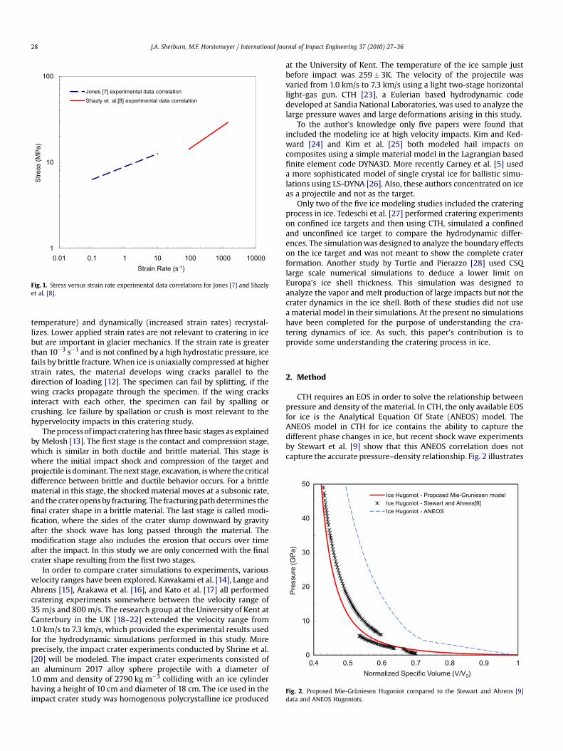
Various studies have documented different aspects of the highrate ice behavior that are related to the constitutive behavior. Langeand Ahrens [6] studied the dynamic tensile strength (17 MPa) of iceat a strain rate of 2�104 s�1. Perhaps the most relevant studiespertaining to the strength of ice was conducted by Jones [7] andShazly et al. [8]. Jones [7] showed in uniaxial compression tests oncolumnar-grained ice at 262 K for strain rates between 0.1 s�1 and10 s�1 the compressive strength of ice increased from approxi-mately 6.3 MPa to 12.6 MPa. Using a Split Pressure Hopkinson Bar(SPHB), Shazly et al. [8] found the increase of compressive strengthfrom 11.7 MPa to 58.4 MPa for higher strain rates (90–1400 s�1).The ice used in Shazly et al. [8] and considered in this study waspolycrystalline ice at 263 K, which had a grain size between 1 and3 mm. The SPHB apparatus is a high strain rate uniaxial compres-sion test. To date, Shazly et al. [8] showed the highest strain ratestress–strain responses in the literature, which were used todevelop the material model in this study. Fig. 1 displays theexperimental data correlations for Jones [7] and Shazly et al. [8].

In addition to a constitutive model, the crater ice simulationsrequire an Equation of State (EOS) to define the relationshipbetween pressure and material density. For this study, a new Mie-Gruniesen EOS was developed and correlated to the experimentalshock wave data for polycrystalline ice garnered by Stewart andAhrens [9–11].

For fracture of ice, Petrenko and Whitworth [12] provide themost thorough review. At low strain rates 10�7 s�1 to 10�3 s�1, ice isductile and deforms plastically by glide and climb from dislocationsmoving in essentially an HCP crystal. Ice also statically (increased

mailto:[email protected]

www.sciencedirect.com/science/journal/0734743X

http://www.elsevier.com/locate/ijimpeng

1

10

100

0.01 0.1 1 10 100 1000 10000

Stre

ss (M

Pa)

Strain Rate (s-1)

Jones [7] experimental data correlationShazly et. al,[8] experimental data correlation

Fig. 1. Stress versus strain rate experimental data correlations for Jones [7] and Shazlyet al. [8].

0

10

20

30

40

50

0.4 0.5 0.6 0.7 0.8 0.9 1

Pres

sure

(GPa

)

Normalized Specific Volume (V/V0)

Ice Hugoniot - Proposed Mie-Gruniesen modelIce Hugoniot - Stewart and Ahrens[9]Ice Hugoniot - ANEOS

Fig. 2. Proposed Mie-Gruniesen Hugoniot compared to the Stewart and Ahrens [9]data and ANEOS Hugoniots.

J.A. Sherburn, M.F. Horstemeyer / International Journal of Impact Engineering 37 (2010) 27–3628

temperature) and dynamically (increased strain rates) recrystal-lizes. Lower applied strain rates are not relevant to cratering in icebut are important in glacier mechanics. If the strain rate is greaterthan 10�3 s�1 and is not confined by a high hydrostatic pressure, icefails by brittle fracture. When ice is uniaxially compressed at higherstrain rates, the material develops wing cracks parallel to thedirection of loading [12]. The specimen can fail by splitting, if thewing cracks propagate through the specimen. If the wing cracksinteract with each other, the specimen can fail by spalling orcrushing. Ice failure by spallation or crush is most relevant to thehypervelocity impacts in this cratering study.

The process of impact cratering has three basic stages as explainedby Melosh [13]. The first stage is the contact and compression stage,which is similar in both ductile and brittle material. This stage iswhere the initial impact shock and compression of the target andprojectile is dominant. The next stage, excavation, is where the criticaldifference between brittle and ductile behavior occurs. For a brittlematerial in this stage, the shocked material moves at a subsonic rate,and the crater opens by fracturing. The fracturing path determines thefinal crater shape in a brittle material. The last stage is called modi-fication, where the sides of the crater slump downward by gravityafter the shock wave has long passed through the material. Themodification stage also includes the erosion that occurs over timeafter the impact. In this study we are only concerned with the finalcrater shape resulting from the first two stages.

In order to compare crater simulations to experiments, variousvelocity ranges have been explored. Kawakami et al. [14], Lange andAhrens [15], Arakawa et al. [16], and Kato et al. [17] all performedcratering experiments somewhere between the velocity range of35 m/s and 800 m/s. The research group at the University of Kent atCanterbury in the UK [18–22] extended the velocity range from1.0 km/s to 7.3 km/s, which provided the experimental results usedfor the hydrodynamic simulations performed in this study. Moreprecisely, the impact crater experiments conducted by Shrine et al.[20] will be modeled. The impact crater experiments consisted ofan aluminum 2017 alloy sphere projectile with a diameter of1.0 mm and density of 2790 kg m�3 colliding with an ice cylinderhaving a height of 10 cm and diameter of 18 cm. The ice used in theimpact crater study was homogenous polycrystalline ice produced

at the University of Kent. The temperature of the ice sample justbefore impact was 259� 3K. The velocity of the projectile wasvaried from 1.0 km/s to 7.3 km/s using a light two-stage horizontallight-gas gun. CTH [23], a Eulerian based hydrodynamic codedeveloped at Sandia National Laboratories, was used to analyze thelarge pressure waves and large deformations arising in this study.

To the author’s knowledge only five papers were found thatincluded the modeling ice at high velocity impacts. Kim and Ked-ward [24] and Kim et al. [25] both modeled hail impacts oncomposites using a simple material model in the Lagrangian basedfinite element code DYNA3D. More recently Carney et al. [5] useda more sophisticated model of single crystal ice for ballistic simu-lations using LS-DYNA [26]. Also, these authors concentrated on iceas a projectile and not as the target.

Only two of the five ice modeling studies included the crateringprocess in ice. Tedeschi et al. [27] performed cratering experimentson confined ice targets and then using CTH, simulated a confinedand unconfined ice target to compare the hydrodynamic differ-ences. The simulation was designed to analyze the boundary effectson the ice target and was not meant to show the complete craterformation. Another study by Turtle and Pierazzo [28] used CSQlarge scale numerical simulations to deduce a lower limit onEuropa’s ice shell thickness. This simulation was designed toanalyze the vapor and melt production of large impacts but not thecrater dynamics in the ice shell. Both of these studies did not usea material model in their simulations. At the present no simulationshave been completed for the purpose of understanding the cra-tering dynamics of ice. As such, this paper’s contribution is toprovide some understanding the cratering process in ice.

2. Method

CTH requires an EOS in order to solve the relationship betweenpressure and density of the material. In CTH, the only available EOSfor ice is the Analytical Equation Of State (ANEOS) model. TheANEOS model in CTH for ice contains the ability to capture thedifferent phase changes in ice, but recent shock wave experimentsby Stewart et al. [9] show that this ANEOS correlation does notcapture the accurate pressure–density relationship. Fig. 2 illustrates

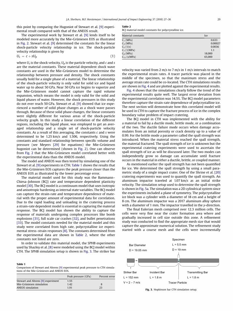
Table 2BCJ material model constants for polycrystalline ice.

Material constants Ice

C1 (MPa) 0.633C3 (MPa) 0.00027C5 (1/s) 0.0036C7 (1/MPa) 1.1C9 (MPa) 18,000C11 (s/MPa) 65,000

Specimen

L = 5.5 mm

D = 19 mmBar Diameter

D = 19.05 mm

J.A. Sherburn, M.F. Horstemeyer / International Journal of Impact Engineering 37 (2010) 27–36 29

this point by comparing the Hugoniot of Stewart et al. [9] experi-mental result compared with that of the ANEOS result.

The experimental work by Stewart et al. [9] lends itself to bemodeled more accurately by the Mie-Gruniesen EOS as illustratedin Fig. 2. Stewart et al. [9] determined the constants for the linearshock-particle velocity relationship in ice. The shock-particlevelocity relationship is given byUs ¼ cþ sUp (1)

where Us is the shock velocity, Up is the particle velocity, and c and sare the material constants. These material dependent shock waveconstants are used in the Mie-Gruniesen model to determine therelationship between pressure and density. The shock constantsusually hold for a single phase of a material. The linear relationshipof the shock-particle velocity is only valid for solid ice and liquidwater up to about 50 GPa. Near 50 GPa ice begins to vaporize andthe Mie-Gruniesen model cannot capture the rapid volumeexpansion, which means the model is only valid for the solid andliquid phases of water. However, the shock pressures in this studydo not ever reach 50 GPa. Stewart et al. [9] showed that ice expe-rienced a number of solid phase changes as a shock wave passesthrough. Because of these solid phase changes, the linear constantswere slightly different for various areas of the shock-particlevelocity graph. In this study a linear correlation of the differentregions, including the liquid phase, was employed to get an aver-aged relationship and a single set of shock-particle velocityconstants. As a result of this averaging, the constants c and s weredetermined to be 1.25 km/s and 1.506, respectively. Using theconstants and standard relationship between specific volume andpressure (see Meyers [29] for equations) the Mie-Gruniesenhugoniot can be determined (shown in Fig. 2). One can observefrom Fig. 2 that the Mie-Gruniesen model correlated better withthe experimental data than the ANEOS model.

The model and ANEOS was then tested by simulating one of theStewart et al. [9] experiments in CTH. Table 1 shows the results thatthe Mie-Gruniesen EOS captures the peak pressure closer than theANEOS EOS as illustrated by the lower percentage error.

The material model used for this study was the Bammann–Chiesa–Johnson (BCJ) rate and temperature dependent plasticitymodel [30]. The BCJ model is a continuum model that uses isotropicand anisotropic hardening as internal state variables. The BCJ modelcan capture the strain-rate and temperature dependence of mate-rial with the proper amount of experimental data for correlation.Due to the rapid loading and unloading in the cratering processa strain-rate dependent model is essential in capturing the materialresponse. The BCJ model has shown the ability to capture theresponse of materials undergoing complex processes like bombexplosions [31], full scale car crashes [32], and bullet penetrations[33]. The model constants needed for the material model and thisstudy were correlated from high rate, polycrystalline ice experi-mental stress–strain responses [8]. The constants determined fromthe experimental data are shown in Table 2, where the otherconstants not listed are zero.

In order to validate this material model, the SPHB experimentsused by Shazley et al. [8] were modeled using the BCJ model withinCTH. The SPHB simulation setup is shown in Fig. 3. The striker bar

Table 1Comparison of Stewart and Ahrens [9] experimental peak pressure to CTH simula-tions of the Mie-Gruniesen and ANEOS EOS.

Peak pressure (GPa) Percent error

Stewart and Ahrens [9] experiment 1.55Mie-Gruniesen simulation 1.42 8ANEOS simulation 1.91 23

velocity was varied from 2 m/s to 7 m/s in 1 m/s intervals to matchthe experimental strain rates. A tracer particle was placed in themiddle of the specimen, so that the maximum stress and theaverage strain rate could be co-located. The CTH simulations resultsare shown in Fig. 4 and are plotted against the experimental results.

Fig. 4 shows that the simulations clearly follow the trend of theexperimental results quite well. The largest error deviation fromthe experimental correlation was 14.5%. The BCJ model parameterstherefore capture the strain-rate dependence of polycrystalline ice.The next section will demonstrate how this correlated model willbe used in CTH to capture the fracture process of ice in the complexboundary value problem of impact cratering.

The BCJ model in CTH was implemented with the ability fora material to fail by a ductile mode, brittle mode, or a combinationof the two. The ductile failure mode occurs when damage accu-mulates from an initial porosity or crack density up to a value of0.99. For the brittle mode a parameter called the spall strength wasintroduced. When the material stress reached the spall strength,the material fractured. The spall strength of ice is unknown but theexperimental cratering experiments were used to ascertain thespall strength of ice as will be discussed later. The two modes canindependently grow so damage can accumulate until fractureoccurs in the material in either a ductile, brittle, or coupled manner.

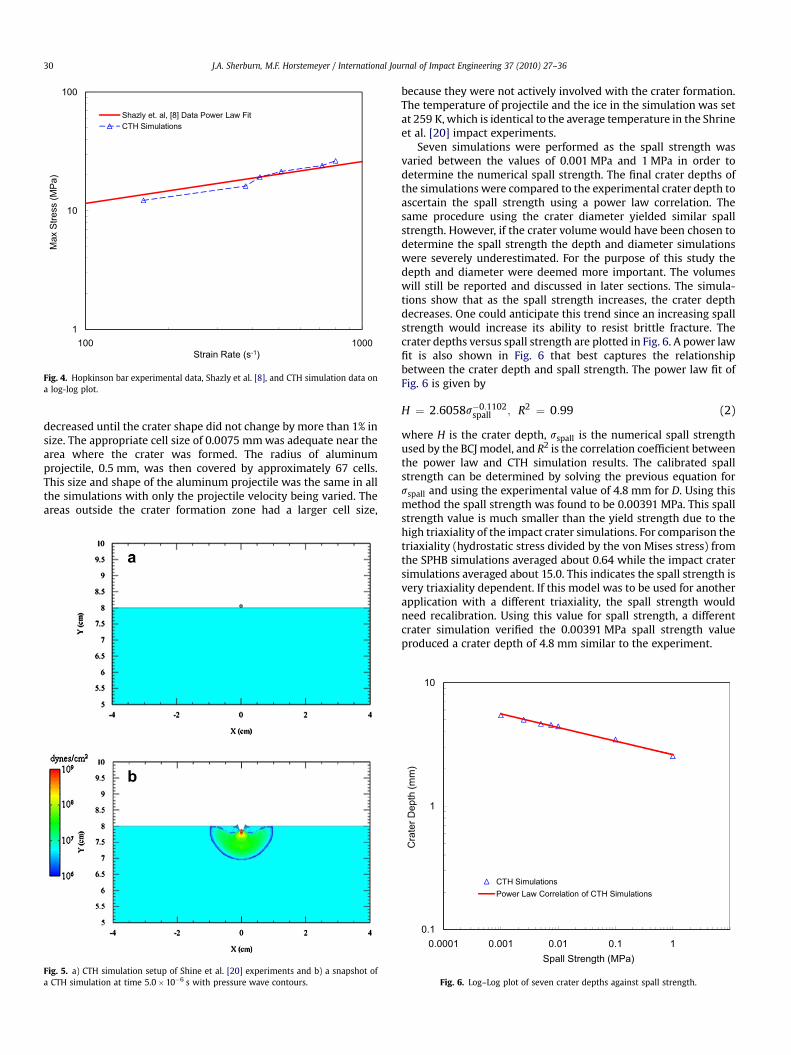
As mentioned earlier the spall strength has not been quantifiedfor ice. We determined the spall strength by using a small para-metric study of a single impact crater. One of the Shrine et al. [20]cratering experiments was used to quantify the spall strength. Analuminum impactor traveled at 1.07 km/s as an initial strikevelocity. The simulation setup used to determine the spall strengthis shown in Fig. 5a. The simulation was a 2D cylindrical system sincethe experiments included a plane of symmetry. The polycrystallineice block was a cylinder with a diameter of 18 cm and a height of8 cm. The aluminum impactor was a 2017 aluminum alloy spherewith a diameter of 1 mm. The impactor travelled in the y-direction.

The final Eulerian mesh comprised over 12.3 million cells. Thecells were very fine near the crater formation area where andgradually increased in cell size outside this zone. A refinementstudy was conducted to find the appropriate mesh size that wouldcapture the approximate numerical solution. The refinement studystarted with a course mesh and the cells were incrementally

Striker Bar

L = 152 mm

V = 2 – 7 m/s

Incident Bar

L = 1.8 m

Transmitting Bar

L = 1.8 m

Tracer Particle

Fig. 3. Hopkinson bar CTH simulation setup.

1

10

100

100 1000

Max

Stre

ss (M

Pa)

Strain Rate (s-1)

Shazly et. al, [8] Data Power Law FitCTH Simulations

Fig. 4. Hopkinson bar experimental data, Shazly et al. [8], and CTH simulation data ona log-log plot.


decreased until the crater shape did not change by more than 1% insize. The appropriate cell size of 0.0075 mm was adequate near thearea where the crater was formed. The radius of aluminumprojectile, 0.5 mm, was then covered by approximately 67 cells.This size and shape of the aluminum projectile was the same in allthe simulations with only the projectile velocity being varied. Theareas outside the crater formation zone had a larger cell size,

Fig. 5. a) CTH simulation setup of Shine et al. [20] experiments and b) a snapshot ofa CTH simulation at time 5.0�10�6 s with pressure wave contours.

because they were not actively involved with the crater formation.The temperature of projectile and the ice in the simulation was setat 259 K, which is identical to the average temperature in the Shrineet al. [20] impact experiments.

Seven simulations were performed as the spall strength wasvaried between the values of 0.001 MPa and 1 MPa in order todetermine the numerical spall strength. The final crater depths ofthe simulations were compared to the experimental crater depth toascertain the spall strength using a power law correlation. Thesame procedure using the crater diameter yielded similar spallstrength. However, if the crater volume would have been chosen todetermine the spall strength the depth and diameter simulationswere severely underestimated. For the purpose of this study thedepth and diameter were deemed more important. The volumeswill still be reported and discussed in later sections. The simula-tions show that as the spall strength increases, the crater depthdecreases. One could anticipate this trend since an increasing spallstrength would increase its ability to resist brittle fracture. Thecrater depths versus spall strength are plotted in Fig. 6. A power lawfit is also shown in Fig. 6 that best captures the relationshipbetween the crater depth and spall strength. The power law fit ofFig. 6 is given by

H ¼ 2:6058s�0:1102spall ; R2 ¼ 0:99 (2)

where H is the crater depth, sspall is the numerical spall strengthused by the BCJ model, and R2 is the correlation coefficient betweenthe power law and CTH simulation results. The calibrated spallstrength can be determined by solving the previous equation forsspall and using the experimental value of 4.8 mm for D. Using thismethod the spall strength was found to be 0.00391 MPa. This spallstrength value is much smaller than the yield strength due to thehigh triaxiality of the impact crater simulations. For comparison thetriaxiality (hydrostatic stress divided by the von Mises stress) fromthe SPHB simulations averaged about 0.64 while the impact cratersimulations averaged about 15.0. This indicates the spall strength isvery triaxiality dependent. If this model was to be used for anotherapplication with a different triaxiality, the spall strength wouldneed recalibration. Using this value for spall strength, a differentcrater simulation verified the 0.00391 MPa spall strength valueproduced a crater depth of 4.8 mm similar to the experiment.

0.1

1

10

0.0001 0.001 0.01 0.1 1

Cra

ter D

epth

(mm

)

Spall Strength (MPa)

CTH SimulationsPower Law Correlation of CTH Simulations

Fig. 6. Log–Log plot of seven crater depths against spall strength.


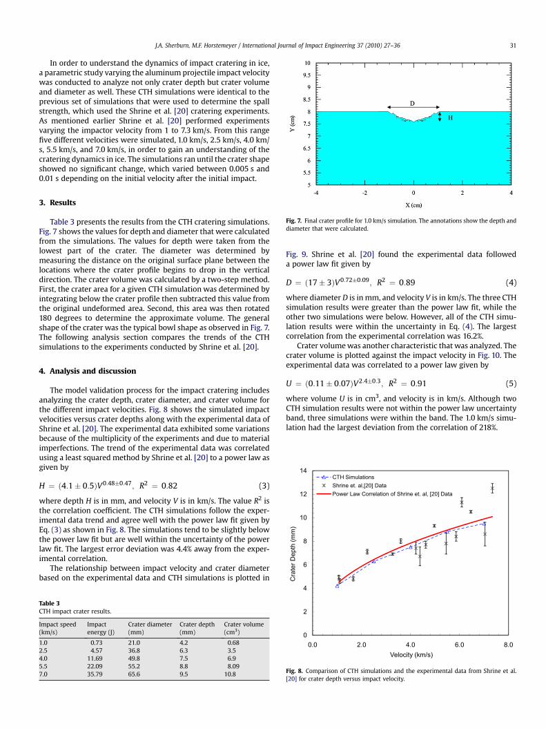
In order to understand the dynamics of impact cratering in ice,a parametric study varying the aluminum projectile impact velocitywas conducted to analyze not only crater depth but crater volumeand diameter as well. These CTH simulations were identical to theprevious set of simulations that were used to determine the spallstrength, which used the Shrine et al. [20] cratering experiments.As mentioned earlier Shrine et al. [20] performed experimentsvarying the impactor velocity from 1 to 7.3 km/s. From this rangefive different velocities were simulated, 1.0 km/s, 2.5 km/s, 4.0 km/s, 5.5 km/s, and 7.0 km/s, in order to gain an understanding of thecratering dynamics in ice. The simulations ran until the crater shapeshowed no significant change, which varied between 0.005 s and0.01 s depending on the initial velocity after the initial impact.

Fig. 7. Final crater profile for 1.0 km/s simulation. The annotations show the depth anddiameter that were calculated.

3. Results

Table 3 presents the results from the CTH cratering simulations.Fig. 7 shows the values for depth and diameter that were calculatedfrom the simulations. The values for depth were taken from thelowest part of the crater. The diameter was determined bymeasuring the distance on the original surface plane between thelocations where the crater profile begins to drop in the verticaldirection. The crater volume was calculated by a two-step method.First, the crater area for a given CTH simulation was determined byintegrating below the crater profile then subtracted this value fromthe original undeformed area. Second, this area was then rotated180 degrees to determine the approximate volume. The generalshape of the crater was the typical bowl shape as observed in Fig. 7.The following analysis section compares the trends of the CTHsimulations to the experiments conducted by Shrine et al. [20].

6

8

10

12

14

Cra

ter D

epth

(mm

)

CTH SimulationsShrine et. al,[20] DataPower Law Correlation of Shrine et. al, [20] Data

4. Analysis and discussion

The model validation process for the impact cratering includesanalyzing the crater depth, crater diameter, and crater volume forthe different impact velocities. Fig. 8 shows the simulated impactvelocities versus crater depths along with the experimental data ofShrine et al. [20]. The experimental data exhibited some variationsbecause of the multiplicity of the experiments and due to materialimperfections. The trend of the experimental data was correlatedusing a least squared method by Shrine et al. [20] to a power law asgiven by

H ¼ ð4:1� 0:5ÞV0:48�0:47; R2 ¼ 0:82 (3)

where depth H is in mm, and velocity V is in km/s. The value R2 isthe correlation coefficient. The CTH simulations follow the exper-imental data trend and agree well with the power law fit given byEq. (3) as shown in Fig. 8. The simulations tend to be slightly belowthe power law fit but are well within the uncertainty of the powerlaw fit. The largest error deviation was 4.4% away from the exper-imental correlation.

The relationship between impact velocity and crater diameterbased on the experimental data and CTH simulations is plotted in

Table 3CTH impact crater results.

Impact speed(km/s)

Impactenergy (J)

Crater diameter(mm)

Crater depth(mm)

Crater volume(cm3)

1.0 0.73 21.0 4.2 0.682.5 4.57 36.8 6.3 3.54.0 11.69 49.8 7.5 6.95.5 22.09 55.2 8.8 8.097.0 35.79 65.6 9.5 10.8

Fig. 9. Shrine et al. [20] found the experimental data followeda power law fit given by

D ¼ ð17� 3ÞV0:72�0:09; R2 ¼ 0:89 (4)

where diameter D is in mm, and velocity V is in km/s. The three CTHsimulation results were greater than the power law fit, while theother two simulations were below. However, all of the CTH simu-lation results were within the uncertainty in Eq. (4). The largestcorrelation from the experimental correlation was 16.2%.

Crater volume was another characteristic that was analyzed. Thecrater volume is plotted against the impact velocity in Fig. 10. Theexperimental data was correlated to a power law given by

U ¼ ð0:11� 0:07ÞV2:4�0:3; R2 ¼ 0:91 (5)

where volume U is in cm3, and velocity is in km/s. Although twoCTH simulation results were not within the power law uncertaintyband, three simulations were within the band. The 1.0 km/s simu-lation had the largest deviation from the correlation of 218%.

0

2

4

0.0 2.0 4.0 6.0 8.0Velocity (km/s)

Fig. 8. Comparison of CTH simulations and the experimental data from Shrine et al.[20] for crater depth versus impact velocity.

0

10

20

30

40

50

60

70

80

90

0.0 2.0 4.0 6.0 8.0

Cra

ter D

iam

eter

(mm

)

Velocity (km/s)


Fig. 9. Comparison of the CTH simulations and the experimental data from Shrineet al. [20] for the crater diameter versus impact velocity.

0.01

0.1

1

10

0.10 1.00 10.00 100.00

Cra

ter V

olum

e (c

m3 )

Impact Energy (J)


Fig. 11. Comparison of the CTH simulations and the experimental data from Shrineet al. [20] for the crater volume versus impact energy.


In addition to the impact velocity and crater volume relation-ship, the impact energy was also of interest in terms of a relation-ship with the crater volume. Fig. 11 shows this relationship forcrater volume versus impact energy for the CTH simulations andthe Shrine et al. [20] experimental data. Fig. 11 gives an indication ofhow much energy it takes to excavate a crater of a given size. Aswith the impact velocity and crater volume plot, Fig. 11 shows thatthree CTH simulation results were within the experimentaluncertainty, while the other two deviate by a small amount.

Another important area of comparison of the CTH simulationresults is with the Shrine et al. [20] dimensionless parameters. Thedimensionless parameters followed the nomenclature of Lange andAhrens [6], who used a similitude variable for scaling created byHolsapple and Schmidt [34]. Taking V and r as the crater volumeand radius, m and v are projectile mass and velocity, respectively;d and r are projectile and target densities, respectively; Y is the

0

2

4

6

8

10

12

14

16

0.0 2.0 4.0 6.0 8.0

Cra

ter V

olum

e (c

m3 )

Velocity (km/s)


Fig. 10. Comparison of the CTH simulations and the experimental data from Shrineet al. [20] for the crater volume versus impact velocity.

target strength; and g is the gravity at the Earth’s surface, the fourdimensionless parameters are defined as the following:

pv ¼ Vr=m; (6)

pr ¼ rðd=mÞ1=3; (7)

p2 ¼ 2gðm=dÞ1=3=v 2; (8)

p3 ¼ Y=dv 2: (9)

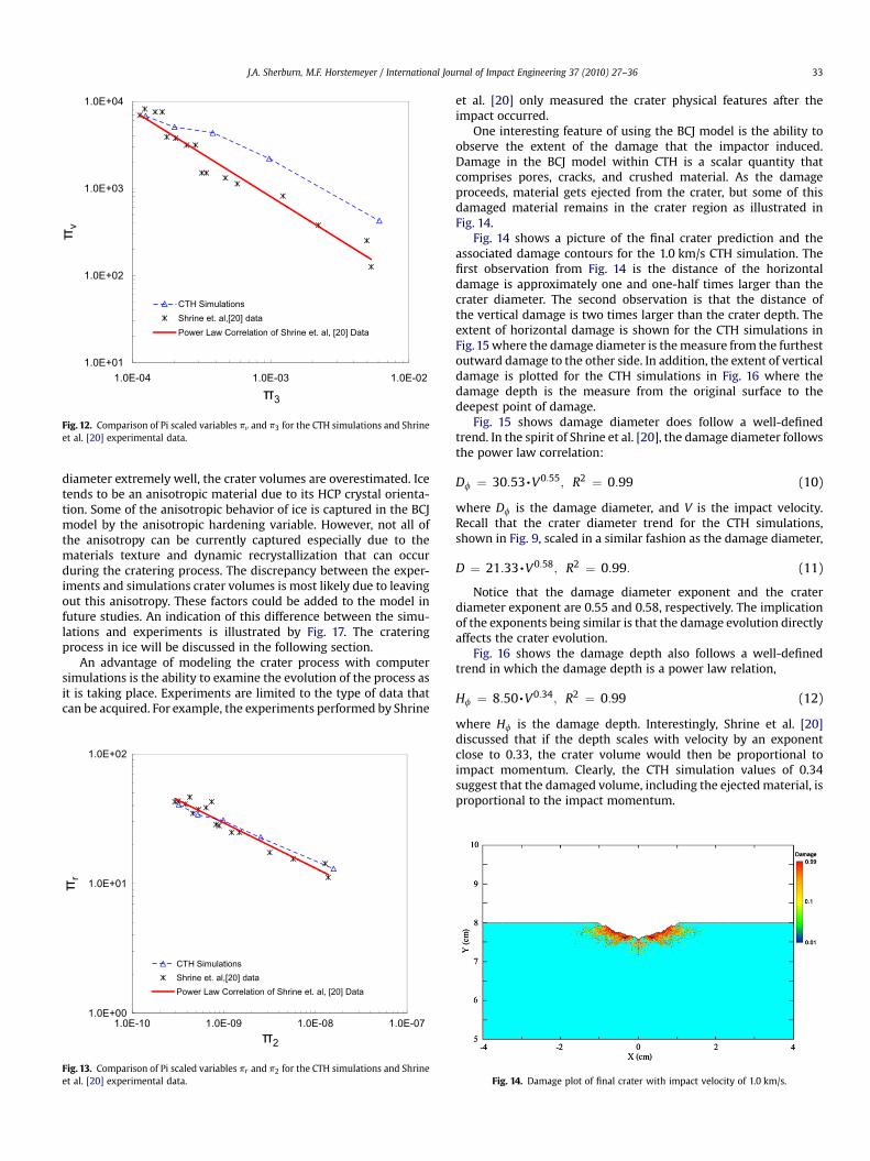
The constants used for Eqs. (6)–(9) are listed in Table 4. Usingthe data from Shrine et al. [20], and the CTH simulation results inthis study, pv are plotted against p3 in Fig. 12, and pr is plottedagainst p2 in Fig. 13. The Pi scaled variable pv is a measure of cra-tering efficiency related to final crater volume, while pr isa measure of cratering efficiency related to the final crater diameter.For consistency with the Shrine et al. [20] data, the value for ice’sstrength from Lange and Ahrens [6] is used for Y (Y¼ 17 MPa). Thevalue of Y from Lange and Ahrens [6] is a measured dynamic tensilestrength. Fig. 12 shows that the CTH simulation results deviatedfrom the experiments for the higher values of p3, which corre-sponded to the lowest impact velocities. The higher simulationvalues of p3 departed from the experiments due to higher cratervolumes in the CTH simulations as illustrated in Fig. 10. However,the CTH simulation results shown in Fig. 13 match well to theexperimental data, because the CTH simulation crater diametersclosely followed the experiments as shown in Fig. 9.

The close comparisons of the CTH simulation results with theexperiments by Shrine et al. [20] validate this study’s model incapturing the general characteristics of impact cratering in ice.Although the model has the ability to capture ice crater depth and

Table 4Values of constants used in Pi scaled variables.

Constant Value

Projectile density (g/cm3) 2.79Target density (g/cm3) 0.917Projectile mass (g) 1.46� 10�3

Gravity (cm/s2) 980Target strength (g/s2 cm) 1.7� 108

1.0E+01

1.0E+02

1.0E+03

1.0E+04

1.0E-04 1.0E-03 1.0E-02

v

3

CTH SimulationsShrine et. al,[20] dataPower Law Correlation of Shrine et. al, [20] Data

Fig. 12. Comparison of Pi scaled variables pv and p3 for the CTH simulations and Shrineet al. [20] experimental data.


diameter extremely well, the crater volumes are overestimated. Icetends to be an anisotropic material due to its HCP crystal orienta-tion. Some of the anisotropic behavior of ice is captured in the BCJmodel by the anisotropic hardening variable. However, not all ofthe anisotropy can be currently captured especially due to thematerials texture and dynamic recrystallization that can occurduring the cratering process. The discrepancy between the exper-iments and simulations crater volumes is most likely due to leavingout this anisotropy. These factors could be added to the model infuture studies. An indication of this difference between the simu-lations and experiments is illustrated by Fig. 17. The crateringprocess in ice will be discussed in the following section.

An advantage of modeling the crater process with computersimulations is the ability to examine the evolution of the process asit is taking place. Experiments are limited to the type of data thatcan be acquired. For example, the experiments performed by Shrine

1.0E+00

1.0E+01

1.0E+02

1.0E-10 1.0E-09 1.0E-08 1.0E-07

r

2

CTH SimulationsShrine et. al,[20] dataPower Law Correlation of Shrine et. al, [20] Data

Fig. 13. Comparison of Pi scaled variables pr and p2 for the CTH simulations and Shrineet al. [20] experimental data.

et al. [20] only measured the crater physical features after theimpact occurred.

One interesting feature of using the BCJ model is the ability toobserve the extent of the damage that the impactor induced.Damage in the BCJ model within CTH is a scalar quantity thatcomprises pores, cracks, and crushed material. As the damageproceeds, material gets ejected from the crater, but some of thisdamaged material remains in the crater region as illustrated inFig. 14.

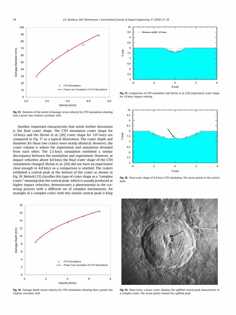
Fig. 14 shows a picture of the final crater prediction and theassociated damage contours for the 1.0 km/s CTH simulation. Thefirst observation from Fig. 14 is the distance of the horizontaldamage is approximately one and one-half times larger than thecrater diameter. The second observation is that the distance ofthe vertical damage is two times larger than the crater depth. Theextent of horizontal damage is shown for the CTH simulations inFig. 15 where the damage diameter is the measure from the furthestoutward damage to the other side. In addition, the extent of verticaldamage is plotted for the CTH simulations in Fig. 16 where thedamage depth is the measure from the original surface to thedeepest point of damage.

Fig. 15 shows damage diameter does follow a well-definedtrend. In the spirit of Shrine et al. [20], the damage diameter followsthe power law correlation:

Df ¼ 30:53,V0:55; R2 ¼ 0:99 (10)

where Df is the damage diameter, and V is the impact velocity.Recall that the crater diameter trend for the CTH simulations,shown in Fig. 9, scaled in a similar fashion as the damage diameter,

D ¼ 21:33,V0:58; R2 ¼ 0:99: (11)

Notice that the damage diameter exponent and the craterdiameter exponent are 0.55 and 0.58, respectively. The implicationof the exponents being similar is that the damage evolution directlyaffects the crater evolution.

Fig. 16 shows the damage depth also follows a well-definedtrend in which the damage depth is a power law relation,

Hf ¼ 8:50,V0:34; R2 ¼ 0:99 (12)

where Hf is the damage depth. Interestingly, Shrine et al. [20]discussed that if the depth scales with velocity by an exponentclose to 0.33, the crater volume would then be proportional toimpact momentum. Clearly, the CTH simulation values of 0.34suggest that the damaged volume, including the ejected material, isproportional to the impact momentum.

Fig. 14. Damage plot of final crater with impact velocity of 1.0 km/s.

0

10

20

30

40

50

60

70

80

90

100

0.0 2.0 4.0 6.0 8.0

Dam

age

Dia

met

er (m

m)

Velocity (km/s)


Fig. 15. Diameter of the extent of damage versus velocity for CTH simulations showingthat a power law relation correlates well.

Fig. 17. Comparison of CTH simulation and Shrine et al. [20] experiment crater shapefor 1.0 km/s impact velocity.

Fig. 18. Final crater shape of 4.0 km/s CTH simulation. The arrow points to the centralpeak.


Another important characteristic that needs further discussionis the final crater shape. The CTH simulation crater shape for1.0 km/s and the Shrine et al. [20] crater shape for 1.07 km/s arecompared in Fig. 17 as a typical illustration. The crater depth anddiameter for these two craters were nearly identical. However, thecrater volume is where the experiment and simulation deviatedfrom each other. The 2.5 km/s simulation exhibited a similardiscrepancy between the simulation and experiment. However, atimpact velocities above 4.0 km/s the final crater shape of the CTHsimulations changed Shrine et al. [20] did not have an experimentclose enough to 4.0 km/s so a comparison is omitted. The cratersexhibited a central peak at the bottom of the crater as shown inFig. 18. Melosh [13] classifies this type of crater shape as a ‘‘complexcrater,’’ meaning that the central peak, which is usually produced athigher impact velocities, demonstrates a phenomenon in the cra-tering process with a different set of complex mechanisms. Anexample of a complex crater with this similar central peak is King

0

2

4

6

8

10

12

14

16

18

0 2 4 6 8

Dam

age

Dep

th (m

m)

Velocity (km/s)


Fig. 16. Damage depth versus velocity for CTH simulations showing that a power lawrelation correlates well.

Fig. 19. King Crater, a lunar crater, displays the uplifted central peak characteristic ofa complex crater. The arrow points toward the uplifted peak.


Crater on the backside of the moon shown in Fig. 19. The CTHsimulations showed as the impact velocity increased, the centralpeak height also increased. The central peak heights above thelowest point in the crater for the 4.0 km/s, 5.5 km/s, and 7.0 km/swere 1.40 mm, 1.74 mm, and 2.09 mm, respectively. Also, recallfrom Fig. 10 that the higher two velocities, 5.5 km/s and 7.0 km/s,were close to the experimental crater volumes. The shapeshowever were different. The reason that the simulation cratervolumes were closer was because the central peak decreased thetotal volume of the crater. If the central peak was ejected, then thecrater would be closer to the experimental crater volumes.

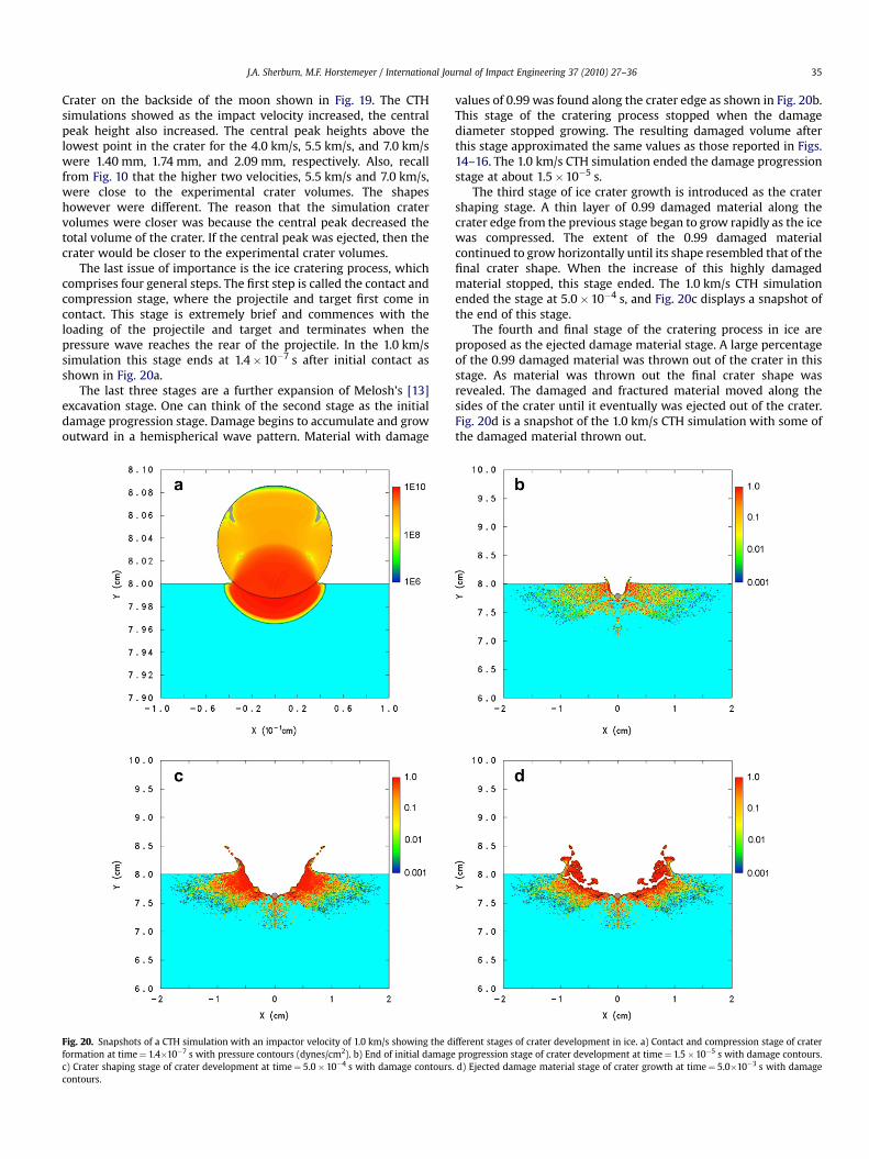
The last issue of importance is the ice cratering process, whichcomprises four general steps. The first step is called the contact andcompression stage, where the projectile and target first come incontact. This stage is extremely brief and commences with theloading of the projectile and target and terminates when thepressure wave reaches the rear of the projectile. In the 1.0 km/ssimulation this stage ends at 1.4�10�7 s after initial contact asshown in Fig. 20a.

The last three stages are a further expansion of Melosh’s [13]excavation stage. One can think of the second stage as the initialdamage progression stage. Damage begins to accumulate and growoutward in a hemispherical wave pattern. Material with damage

Fig. 20. Snapshots of a CTH simulation with an impactor velocity of 1.0 km/s showing the dformation at time¼ 1.4�10�7 s with pressure contours (dynes/cm2). b) End of initial damagec) Crater shaping stage of crater development at time¼ 5.0� 10�4 s with damage contourscontours.

values of 0.99 was found along the crater edge as shown in Fig. 20b.This stage of the cratering process stopped when the damagediameter stopped growing. The resulting damaged volume afterthis stage approximated the same values as those reported in Figs.14–16. The 1.0 km/s CTH simulation ended the damage progressionstage at about 1.5�10�5 s.

The third stage of ice crater growth is introduced as the cratershaping stage. A thin layer of 0.99 damaged material along thecrater edge from the previous stage began to grow rapidly as the icewas compressed. The extent of the 0.99 damaged materialcontinued to grow horizontally until its shape resembled that of thefinal crater shape. When the increase of this highly damagedmaterial stopped, this stage ended. The 1.0 km/s CTH simulationended the stage at 5.0�10�4 s, and Fig. 20c displays a snapshot ofthe end of this stage.

The fourth and final stage of the cratering process in ice areproposed as the ejected damage material stage. A large percentageof the 0.99 damaged material was thrown out of the crater in thisstage. As material was thrown out the final crater shape wasrevealed. The damaged and fractured material moved along thesides of the crater until it eventually was ejected out of the crater.Fig. 20d is a snapshot of the 1.0 km/s CTH simulation with some ofthe damaged material thrown out.

ifferent stages of crater development in ice. a) Contact and compression stage of craterprogression stage of crater development at time¼ 1.5�10�5 s with damage contours.

. d) Ejected damage material stage of crater growth at time¼ 5.0�10�3 s with damage


5. Conclusions

The simulation of impact cratering in ice was investigated inCTH for the velocity range of 1.0–7.0 km/s. In order to study thecratering phenomena in ice, a Mie-Gruniesen equation of statemodel for ice was developed and validated using the recentexperimental data of Stewart and Ahrens [9]. The materialconstants for the Bammann–Cheisa–Johnson plasticity-damagemodel were found and validated using Split Pressure HopkinsonBar (SPHB) experimental data by Shazly et al. [8]. The CTH impactsimulations agreed well with the experimental data of Shrine et al.[20] in terms of crater diameter, depth, volume, and energyabsorption. This validation process provided a basis for under-standing the dynamics of crater development in ice.

One important result of the cratering study was the discoverythat the damaged volume produced by the projectile was directlyproportional to the projectile’s momentum. This could haveimplications for the application of impact penetration in an icybody like an ice sheet or an icy celestial body.

Another important result of the cratering study was the iden-tification of four stages of crater development in ice based upondifferent physical processes. The four proposed stages modifyMelosh’s definition [13] and help isolate the different characteris-tics of the cratering process in ice.

Finally, this study introduces a methodology for studying the icecratering process via hydrodynamic modeling and simulations. Theincorporation of experimental data to determine an internal statevariable plasticity-damage model coupled with spallation can be usedas a basis for solving a boundary value problem like cratering in ice.

Acknowledgements

The authors would like to thank the Center for AdvancedVehicular Systems at Mississippi State University for use of theLinux workstation and processing clusters where the CTH simula-tions for this work were conducted.

References

[1] Arny TT. Explorations: an introduction to astronomy. New York: McGraw-Hill;2002.

[2] Kepler J.Six-corneredsnowflake. Translatedby C Hardie.London: Oxford UP; 1966.[3] Shazly M, Prakash V, Lerch BA. High strain rate compression testing of ice. In:

Proceedings of the 2005 SEM annual conference and exposition on experi-mental and applied mechanics at Portland, Oregon. Bethel, CT: Society ofExperimental Mechanics; 2005. p. 359–65.

[4] Dutta PK, Cole DM, Schulson EM, et al. A fracture study of ice under high strainrate loading. In: Proceedings of the thirteenth international offshore and polarengineering conference at Honolulu, Hawaii. Cupertino, CA: The InternationalSociety of Offshore and Polar Engineers; 2003. p. 465–72.

[5] Carney KS, Benson DJ, DuBois P, et al. A phenomenological high strain ratemodel with failure for ice. Int J Solid Struct 2006;43:7820–39.

[6] Lange MA, Ahrens TJ. The dynamic tensile strength of ice and ice-silicatemixtures. J Geophys Res 1983;88(B2):1197–208.

[7] Jones SJ. High strain-rate compression tests on ice. J Phys Chem B1997;101:6099–101.

[8] Shazly M, Prakash V, Lerch BA. High-strain-rate compression testing of ice.Cleveland, OH: Nasa Glenn Research Center; January 2006. NASA/TM-2006–213966.

[9] Stewart ST, Ahrens TJ. Shock Hugoniot of H2O ice. Geophys Res Lett2003;30(6):1332–5.

[10] Stewart ST, Ahrens TJ. Hugoniots and shock-melting criteria for solid andporous H2O ice. In: Proceedings of the Lunar Planet Sci Conference, vol. 34.League City, TX: Lunar and Planetary Institute; 2003 [abstract 1622].

[11] Stewart ST. Collisional processes involving icy bodies in the solar system. Ph.D.thesis, California Institute of Technology, Pasadena, CA; 2002.

[12] Petrenko VF, Whitworth RW. Physics of ice. Oxford: Oxford UP; 1999.[13] Melosh HJ. Impact cratering: a geologic process. New York: Oxford UP; 1989.[14] Kawakami S, Mizutani H, Takagi Y, et al. Impact experiments on ice. J Geophys

Res 1983;88(B7):5806–14.[15] Lange MA, Ahrens TJ. Impact experiments in low-temperature ice. Icarus

1987;69:506–18.[16] Arakawa M, Higa M, Leliwa-Kopystynski J, Maeno N. Impact cratering of

granular mixture targets made of H2O ice–CO2 ice–pyrophylite. Planet SpaceSci 2000;48:1437–46.

[17] Kato M, Iijima Y-I, Arakawa M, et al. Ice-on-ice impact experiments. Icarus1995;113:423–41.

[18] Burchell MJ, Grey IDS, Shrine NRG. Laboratory investigations of hypervelocityimpact cratering in ice. Adv Space Res 2001;28(10):1521–6.

[19] Burchell MJ, Johnson E, Grey IDS. Hypervelocity impacts on porous ices. In:Warmbein B, editor. Proceedings of asteroids, comets, meteors. Berlin(Germany): ESA Publications Division; 2002. p. 859–62.

[20] Shrine NRG, Burchell MJ, Grey IDS. Velocity scaling of impact craters in waterice over the range 1–7.3 km s�1. Icarus 2002;155:475–85.

[21] Burchell MJ, Leliwa-Kopystynski J, Arakawa M. Cratering of icy target s bydifferent impactors: laboratory experiments and implications for cratering inthe solar system. Icarus 2005;179:274–88.

[22] Burchell MJ, Johnson E. Impact craters on small icy bodies such as icy satellitesand comet nuclei. Mon Not R Astron Soc 2005;360:769–81.

[23] McGlaun JM, Thompson SL, Elrick MG. Cth: a three-dimensional shock wavephysics code. Int J Impact Eng 1990;10:351–60.

[24] Kim H, Kedward KT. Modeling hail ice impacts and predicting impact damageinitiation in composite structures. AIAA J 2000;38(7):1278–88.

[25] Kim H, Welch DA, Kedward KT. Experimental investigation of high velocity iceimpacts on woven carbon/epoxy composite panels. Composites A App Sci Man2003;34:25–41.

[26] Hallquist JO. ls-dyna theoretical manual. Tech. Rep., livermore softwaretechnology corporation; 1998.

[27] Tedeschi WJ, Remo JL, Schulze JF, et al. Experimental hypervelocity impacteffects on simulated planetesimal materials. Int J Impact Eng 1995;17:837–48.

[28] Turtle EP, Pierazzo E. Thickness of a Europan ice shell from impact cratersimulations. Science 2001;294:1326–8.

[29] Meyers MA. Dynamic behavior of materials. New York: John Wiley & Sons Inc.;1994.

[30] Bammann DJ. Modeling the temperature and strain rate dependent largedeformation of metals. App Mech Rev 1990;43(2):S312–9. Part 2.

[31] Bammann DJ, Chiesa ML, Horstemeyer MF, et al. Failure in ductile materialsusing finite element methods. In: Wierzbicki T, Jones N, editors. Structuralcrashworthiness and failure. Belfast: Elsevier Applied Science, The UniversitiesPress; 1993.

[32] Fang H, Solanki K, Horstemeyer MF. Numerical simulations of multiple vehiclecrashes and multidisciplinary crashworthiness optimization. Int J Crashwor-thiness 2005;10(2):161–71.

[33] Horstemeyer MF, Revelli V. In: McDowell DL, editor. Stress history dependentlocalization and failure using continuum damage mechanics concepts. ASTM,application of continuum damage mechanics to fatigue and fracture; 1996.STP1315.

[34] Holsapple KA, Schmidt RM. On the scaling of crater dimensions, II. Impactprocesses. J Geophys Res 1982;87:1849–70.

Hydrodynamic modeling of impact craters in ice

Documents

Transcript of Hydrodynamic modeling of impact craters in ice