GRAVITY AND ARCH DAMS INCLUDING HYDRODYNAMIC ...

REPORT NO.

UCB/EERC-80/39

OCTOBER 1980

PNH-152324

EARTHQUAKE ENGINEERING RESEARCH CENTER

DYNAMIC RESPONSE OFEMBANKMENT CONCRETEGRAVITY AND ARCH DAMSINCLUDING HYDRODYNAMICINTERACTIONby

JOHN F. HALL

ANIL K. CHOPRA

A Report on Research Conducted underGrants ATA74-20554 and ENV76-80073from the National Science Foundation.

COLLEGE OF ENGINEERING

UNIVERSITY OF CALIFORNIA . Berkeley, California-IlEPllODUCEDBYNATIONAL TECHNICALINFORMATION -SERVICE

u.s. DEPARTMENT Of COMMERCESPRIIIGfIElD. VA 22161

DISCLAIMER

Any opinions, findings, and conclusions or

recommendations expressed in this publication are those of the authors and do not

necessarily reflect the views of the National

Science Foundation or the Earthquake En

gineering Research Center, University of

California, Berkeley.

For sale by the National Technical Information Service, U.S. Department of Commerce,Springfield, Virginia 22161.

See back of report for up to date listing ofEERC reports.

502n-l01

REPORT DOCUMENTATION 11. REPORT NO.

PAGE NSF/RA-80 0298•• Title and Subtitle

Dynamic Response of Embankment Concrete-Gravity and Arch DamsIncluding Hydrodynamic Interaction

7. Author{s)

John F. Hall and Anil K. Chopra9. Performing Organization Name and Address

Earthquake Engineering Research CenterUniversity of California, BerkeleyRichmond Field Station47th Street &Hoffman BoulevardRichmond, Calif. 94804

12. Sponsoring Organization Name and Address

National Science foundation1800 G. Street, N.W.Washington, D.C. - 20550

15. Supplementary Notes

3. Recipient's Accession No.

PIIl1 1 I) 23 2 •5. Report Date

October, 1980

8. Performlna: Organization Rept. No.

UCB/EERC-80/3910. Proje<:t/TasklWork Unit No.

11. Contract(C) Or Grant{G) No.

(C)

(G)

13. TyP4l 0' Report & Period Covered

14.

16. Abstract (Limit: 200 words)

An analysis procedure in the frequency domain is developed for determining the earthquake response of a dam including hydrodynamic interaction and water compressibilityeffects. Linear responses of idealized, two-dimensional gravity dams and threedimensional dams, including arch dams, can be obtained. The dam and fluid domain aretreated as substructures and modeled with finite elements. The only geometric restrictionis that an infinite fluid domain must maintain a uniform cross-section beyond some pointin the upstream direction. For such an infinite uniform region, a finite elementdiscretization within the cross-section combined with a continuum representation inthe infinite direction provides for a proper transmission of pressure waves. The fluiddomain model approximately accounts for fluid-foundation interaction through a dampingboundary condition applied along the reservoir floor and sides. The dam foundation isassumed rigid.

Hydrodynamic effects are shown to be equivalent to an added mass and added load in thefrequency domain equations of motion of the dam.

Hydrodynamic effects on the dam response are investigated for acceleration responses toharmonic ground motions. Complex frequency response functions for-acceleration at thedam crest are presented for two-dimensional concrete gravity and earth dams and for athree-dimensional arch dam. Several reservoir shapes are included for the concretegravity dams. Water compressibility and fluid-foundation interaction significantlyinfluence the response of concrete gravity dams and are even more important for the archdam. One effect is a greatly increased importance for the vertical component of groundmotion. Hydrodynamic effects on the responses of earth dams are shown to be minor.

18. Availability Stateme,,:

Release Unlimited

(See ANSI-Z39.18)

19. Seeurity Class (ThIs Report)

20. SKurit)l Clns (This Paae)

s.. IlIstruct,OIlS 011 Reverse

:it. No. 0' PaBe5

24622. Price

OFTJONAL FORM 2n (4-77)(Formerly NTlS-3S)Department of Commerce

DYNAMIC RESPONSE OF EMBANKMENT, CONCRETE-GRAVITY AND ARCH DAMS

INCLUDING HYDRODYNAMIC INTERACTION

by

John F. Hall

Anil K. Chopra

A Report on Research Conducted UnderGrants ATA74-20554 and ENV76-80073

from the National Science Foundation

Report No. UCB/EERC-80/39Earthquake Engineering Research Center

University of CaliforniaBerkeley, California

October 1980

ABSTRACT

An analysis procedure in the frequency domain is developed for

determining the earthquake response of a dam including hydrodynamic

interaction and water compressibility effects. Linear responses of

. idealized, two-dimensional gravity dams and three-dimensional dams,

including arch dams, can be obtained. The dam and fluid domain are

treated as substructures and modeled with finite elements. The only

geometric restriction is that an infinite fluid domain must maintain

a uniform cross-section beyond some point in the upstream direction.

For such an infinite uniform region, a finite element discretization

within the cross-section combined with a continuum representation in

the infinite direction provides for a proper transmission of pressure

waves. The fluid domain model approximately accounts for fluid

foundation interaction through a damping boundary condition applied

along the reservoir floor and sides. The dam foundation is assumed

rigid.

Hydrodynamic effects are shown to be equivalent to an added

mass and added load in the frequency domain equations of motion of the

dam. When water compressibility is considered, the added mass and

added load vary with excitation frequency, and factors influencing

the dam response include resonances of the added load and the radia

tion damping associated with the imagi~ary component of the added mass.

If fluid-foundation interaction is neglected, this damping occurs only

for infinite fluid domains, but occcurs for both infinite and finite

fluid domains if fluid-foundation interaction is included.

i i

Fluid-foundation interaction also reduces resonances of the added load

which can be very large if the foundation beneath the water is assumed

rigid.

Hydrodynamic effects on the dam response are investigated for

acceleration responses to harmonic ground motions. Complex frequency

.response functions for acceleration at the dam crest are presented for

two-dimensional concrete gravity and earth dams and for a three

dimensional arch dam. Several reservoir shapes are included for the

concrete gravity dams. Water compressibility and fluid-foundation

interaction significantly influence the response of concrete gravity

dams and are even more important for the arch dam. One effect is a

greatly increased importance for the vertical component of ground

motion. Hydrodynamic effects on the responses of earth dams are shown

to be minor.

iii

ACKNOWLEDGEMENT

This research investigation was supported by the National Science

Foundation under Grants ATA74-20554 and ENV76-80073. The authors are

grateful for this support.

This report also constitutes John F. Hall's doctoral dissertation

which has been submitted to the University of California, Berkeley.

The dissertation committee consisted of Professors A. K. Chopra

(Chairman), R. W. Clough and B. A. Bolt. Appreciation is expressed to

Professors Clough and Bolt for reviewing the manuscript.

v

TABLE OF CONTENTS

ABSTRACT . . . .

ACKNOWLEDGEMENTS

TABLE OF CONTENTS

1. INTRODUCTION.

1.1 Objectives

1.2 Background

1.3 Scope. . .

2. TWO-DIMENSIONAL ANALYSIS PROCEDURE FOR DAM RESPONSE

2.1 Systems and Ground Motion .....••...

2.2 Equations of Motion for Rigid Foundation Case.

2.2.1 Dam .•

2.2.2 Fluid

2.3 Response to Harmonic Ground Motion

2.4 Response to Arbitrary Ground Motions

2.5 Modifications to Include Fluid-Foundation Interaction .

2.5.1 One-dimensional fluid-foundation system

2.5.2 Two-dimensional fluid-foundation systems .

3. TWO-DIMENSIONAL ANALYSIS OF HYDRODYNAMIC FORCE VECTORS .

3.1 Boundary Value Problems and Solution Techniques.

3.2 Finite Fluid Domains of Irregular Geometry

3.3 Infinite Fluid Domain of Constant Depth .

3.3.1 Boundary value problems

3.3.2 First B.V.P. • .•.

3.3.3 Second B.V.P.

3.4 Infinite Fluid Domains of Irregular Geometry

Preceding page blank

Page

i

iii

v

1

1

4

7

7

9

9

13

14

18

20

20

25

29

29

33

36

36

38

43

46

vi

3.5 Computation of Hydrodynamic Force Vectors .

3.6 Numerical Results ..•..

Page

50

51

3.6.1 Infinite fluid domain of constant depth 51

3.6.2 Infinite fluid domain with sloped dam-fluidinterface . . . . . . . . . . . . . . . 62

4. HYDRODYNAMIC EFFECTS IN RESPONSE OF CONCRETE GRAVITY DAMS 65

4.1 Systems, Ground Motion, and Outline of Analysis 65

4.2 Hydrodynamic Forces on Rigid Dams ...

4.2.1 Water compressibility effects

68

70

4.2.2 Partial vertical excitation of the reservoirfloor . . . . . . . . . . . . . . . 75

4.2.3 Fluid-foundation interaction effects 75

4.3 Dam Responses to Hori zonta1 Ground Motion 77

4:3.1 Dam-fluid interaction effects

4.3.2 Fluid-foundation interaction effects.

4.4 Dam Responses to Vertical Ground Motion ..

4.4.1 Dam-fluid interaction effects

77

80

81

83

4.4.2 Partial vertical excitation of the reservoirfloor.. . . . . . . . . . . . . 85


5. HYDRODYNAMIC EFFECTS IN RESPONSE OF EARTH DAMS 89

5.1 System Considered and Outline of Analysis

5.2 Hydrodynami c Forces on a Ri·gi d Dam .


5.2.2 Fluid-foundation interaction effects

89

92

94

96

vii

5.3 Responses of the Dam . . . . . . • .


Page

96

98


6. THREE-DIMENSIONAL ANALYSIS PROCEDURE FOR DAM RESPONSE . 101

6.1 Systems and Ground Motion . . . . . . . . . .. .. 101

6.2 Response to Harmonic Ground Motion Neglecting FluidFoundation Interaction . . . . . . • . . . . . . .. 101

6.3 Modifications to Include Fluid-Foundation Interaction 107

7. THREE-DIMENSIONAL ANALYSIS OF HYDRODYNAMIC FORCE VECTORS . 109

7.1 Boundary Value Problems and Solution Techniques . 109

7.2 Finite Fluid Domains of Irregular Geometry 111

7.3 Infinite Fluid Domains of Uniform Cross-Section 114

7.B.l Boundary value problems.

7.3.2 First B.V.P.

7.3.3 Second B.V.P.


7.5 Computation of Hydrodynamic Force Vectors .

8. HYDRODYNAMIC EFFECTS IN RESPONSE OF MORROW POINT DAM


8.2 Hydrodynamic Forces on a Rigid Dam ..

8.2.1 Water compressibility effects.


8.3 Responses of the Dam .

114

116

119

• 121

124

· . 127

127

· . 132

· . 132

139

· . 139

8.3. 1

8.3.2

9. CONCLUS IONS

REFERENCES

viii

Dam-fluid interaction effects . . ...

Fluid-foundation interaction effects

Page

143

145

149

155

APPENDIX A. NOTATION 157

APPENDIX B. FINITE ELEMENT DERIVATIONS FOR FINITE FLUIO ODrifAINS 165

APPENDIX C. BOUNDARY CONDITIONS FOR INFINITE FLUID DOMAINS 187

APPENDIX D. BOUNDARY COMPUTATIONS FOR FINITE FLUID DOMAINS 195

APPENDIX E. CONTINUUM SOLUTION FOR THE INFINITE FLUID DOMAINOF CONSTANT DEPTH . . . . . . . . • . . . . . .. 207

APPENDIX F. COMPUTATIONAL D~TAILS

LIST OF EERe REPORTS

. . . . . . . . . . . . . . 217

1. INTRODUCTION

1.1 Objectives

The impounded water may significantly influence the dynamic

response of dams subjected to earthquake ground motions. Present

. analysis capabilities for dam response considering hydrodynamic inter

action are limited because portions of the analysis dealing with the

fluid domain are inefficient except for a few~ simple geometries. An

objective of this work is the ~eve10pment of an analysis procedure

which can efficiently handle an arbitrary fluid domain geometry,

either finite or infinite, and either two or three-dimensional. This

procedure will then be used to further the study of hydrodynamic

effects on the dynamic response of two-dimensional gravity dams and

three-dimeDsiona1 arch dams.

2

programs. The program ADAP (1) contains features pertinent to arch

dam analysis such as special shell elements and mesh generation

capabilities. Alternatively, the frequency domain version of the

equations of motion can be solved and the resulting frequency

responses of the dam converted to the time domain by Fourier trans

form procedures. The frequency responses generated by this method

are useful for identifying aspects of structural response behavior.

If water is present in the reservoir, it should be included in

the analysis. This problem is an interactive one; dam motions are

affected by the hydrodynamic pressures, and these pressures are gen

erated in part by the dam motions. Further, water compressibility

influences the earthquake response of dams (2,3). Successful analyses

have been performed by the method of substructures in which effects

of the fluid are included in the equation of motion of the dam by

addition of hydrodynamic forces which act on the upstream dam face.

These hydrodynamic terms are computed from solutions to the wave

equation over the fluid domain substructure subjected to appropriate

boundary conditions.

The substructure method can be implemented in either the time

domain (4,5) or frequency domain (3,6,7). Explicit mathematical

expressions for the hydrodynamic terms can be employed for simple

fluid domain geometries. For compressible water, such analyses are

most conveniently carried out in the frequency domain, and the result

ing hydrodynamic terms are frequency dependent. Two-dimensional con

crete gravity dam-fluid systems have been successfully treated using

an infinite fluid domain of constant depth (7). More recently, the

method has been applied to arch dam-fluid systems where the infinite

3

reservoir is defined by a cylindrical dam face of constant radius, a

horizontal floor, and vertical, radial banks enclosing a central angle

of 90° (3). Both these analyses efficiently use free vibration mode

shapes of the dam without water as generalized coordinates.

For irregular fluid domain geometries, numerical discretization

techniques are required. Both finite difference (4,5) and finite

element (6) discretization techniques have been used, although finite

elements are better suited to irregular geometries. For compressible

water and an infinite fluid domain, time domain procedures require

very long meshes so that pressure waves reflecting from the upstream

boundary do not return to the dam during the period of analysis.

"Quiet" boundaries which satisfactorily transmit the pressure waves

and which can be placed close to the dam do not seem possible in the

time domain. However, a satisfactory discretization technique for

infinite domains has been developed in the frequency domain for cer

tain problems of solid mechanics involving layered media (8). This

technique is more efficient and also more accurate than those employ

ing infinite elements (6).

Foundation flexibility is another complicating factor, and

both the dam and fluid interact with the foundation. Inclusion of

foundation flexibility requires specification of free-field ground

motions (those motions at the dam and fluid boundaries if the dam and

fluid were absent) and incorporation of an appropriate mechanism to

radiate energy into the foundation. The most extensive implementation

of these features considers the two-dimensional gravity dam with the

infinite fluid domain of constant depth and an elastic half-space

foundation (9). Relatively little has been reported for three-

4

dimensional arch dam-fluid systems because of the complicated geometry

of the foundations. However~ a boundary condition has been employed

along the portion of the foundation adjacent to the fluid which absorbs

a portion of the incident energy associated with a pressure wave strik

ing this boundary (5). An equivalent form of this boundary condition

has also been used to modify hydrodynamic pressures generated by the

vertical component of ground motion (3,7,9,10).

1.3 Scope

An analysis procedure is developed for determining the earth

quake response of a dam, assumed to be linearly elastic, including

interactive and water compressibility effects. The procedure can han

dle the rigid foundation case, but also includes a more general form

of the boundary condition (5) which approximately accounts for inter

action between the fluid and the foundation. The analysis procedure

is a generalization of the substructure approach (3,7) to arbitrary

two and three-dimensional geometries. Finite element techniques are

employed for both the dam and fluid domain substructures. The only

geometric restriction is that an infinite fluid domain must maintain

a uniform cross-section beyond some point in the upstream direction.

For such a fluid domain, an adaptation of a procedure dealing with an

infinite soil layer and the transmission of Love waves (8) provides a

satisfactory and efficient solution technique.

Chapters 2 to 5 deal with two-dimensional dam-fluid systems and

Chapters 6 to 8 with three-dimensional systems. In Chapter 2, the

frequency domain equations of motion of the dam including frequency

dependent hydrodynamic terms are written for two-dimensional gravity

5

dam-fluid systems subjected to horizontal and vertical ground motions.

Equations of motion of the fluid domain including appropriate boundary

conditions are also presented. Finite element analysis procedures for

these equations are described in Chapter 3 for finite and i'nfinite

fluid domains. Computation of the hydrodynamic terms from the result

ing pressures along the dam-fluid interface is also discussed. In

Chapters 4 and 5. the effects of presence of water, compressibility

of water. fluid domain shape, fluid-foundation interaction, and

direction of ground motion on the responses of concrete and earth

gravity dams, respectively, are investigated. Frequency response

functions for the dam crest acceleration and the hydrodynamic force

on a rigid dam are presented. Chapters 6 and 7 generalize the analy

sis procedures of Chapters 2 and 3 to three-dimensional dam-fluid

systems. An analysis of Morrow Point Dam, an arch dam, is presented

in Chapter 8 where effects of presence of water, compressibility of

water, fluid-foundation interaction, and direction of ground motion

are investigated.

7

2. TWO-DIMENSIONAL ANALYSIS PROCEDURE FOR DAM RESPONSE

2.1 Systems and Ground Motion

Concrete gravity dams are treated as two-dimensional systems in

which the planar vibration of individual monoliths of a dam are con

sidered (Fig. 2.1a). This simplification appears to be reasonable

because, at large amplitudes of motion, the monoliths tend to vibrate

independently (11). Each monolith is assumed to be in plane stress.

An earth or rockfill dam with a length several times its cross

sectional dimensions may be idealized to be in plane strain, thus

reducing it to a two-dimensional system (Fig. 2.1b). The plane strain

assumption is also applicable to the water if the valley cross-section

is wide and if the variation in dam motion is small along its length.

These two-dimensional idealizations are not capable of considering

cross-stream components of ground motion. Behaviors within the elas

tic dam and compressible water are assumed linear.

The reservoir may extend only a short distance upstream

(Fig. 2.1b) or to a large enough distance so that it can be assumed

infinite for purposes of analysis (Fig. 2.1a). In the latter case, a

convenient assumption is that the reservoir floor is horizontal beyond

some point in the upstream direction.

The base of the dam and reservoir floor in Fig. 2.1 undergo a

prescribed acceleration time history described by the horizontal and

vertical (x and y) components of ground motion. By specifying these

accelerations of the fluid boundaries, the foundation is assumed rigid,

and no interaction can take place between the dam and foundation or

between the fluid and foundation. Inclusion of foundation interaction

. Preceding page blank

8

v

WATER

CONSTANTDEPTH

(a) CONCRETE DAM I INFINITE FLUID DOMAIN

y

x

v

WATER

(b) EARTH DAM, FINITE FLUID DOMAIN

FIG. 2.1 TWO-DIMENSIONAL GRAVITY DAM-FLUID SYSTEMS

9

effects requires a flexible foundation model and specification of

free-field accelerations along the dam base and reservoir floor

(those accelerations resulting from the earthquake if the dam and

fluid were absent). A procedure for determining the dynamic response

of the dam on a rigid foundation is described in Sees. 2.2 to 2.4.

Some modifications to this procedure which approximately account for

interaction between the fluid and foundation are discussed in Sec. 2.5.

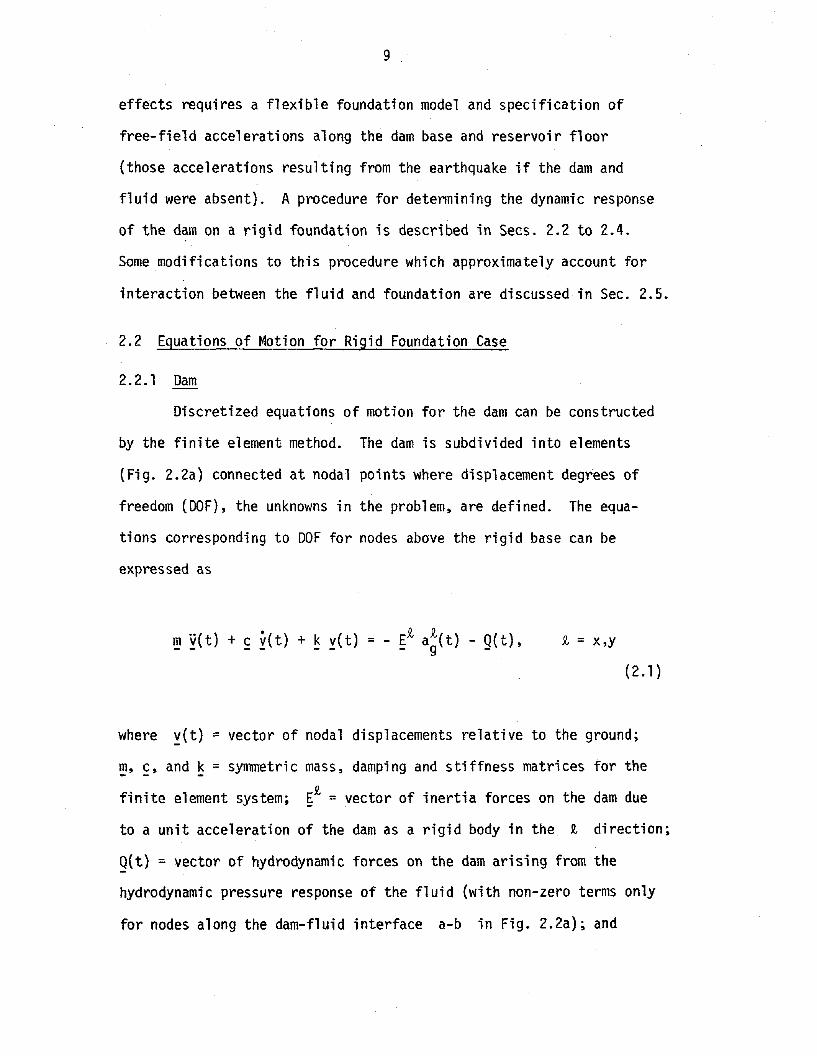
2.2 Equations of Motion for Rigid Foundation Case

2.2.1 Dam

Discretized equations of motion for the dam can be constructed

by the finite element method. The dam is subdivided into elements

(Fig. 2.2a) connected at nodal points where displacement degrees of

freedom (DOF), the unknowns in the problem, are defined. The equa

tions corresponding to OOF for nodes above the rigid base can be

expressed as

fI, = x,y

(2.1 )

where ~(t) = vector of nodal displacements relative to the ground;

~, ~, and k = symmetric mass, damping and stiffness matrices for the

finite element system; ~fI, = vector of inertia forces on the dam due

to a unit acceleration of the dam as a rigid body in the fI, direction;

Q(t) = vector of hydrodynamic forces on the dam arising from the

hydrodynamic pressure response of the fluid (with non-zero terms only

for nodes along the dam-fluid interface a-b in Fig. 2.2a); and

10

d

n s'

(0) FINITE ELEMENT DAM MODEL. INFINITE FLUIDDOMAIN

n

(b) DEFINITION OF e-/(S), 5 =5,5·

FIG. 2.2 IDEALIZED DAM-FLUID SYSTEM, DEFINITIONS AND NOTATION

11

a~(t} is the component of ground acceleration in the R, direction.

ER, is given by

{2.2}

where m = a mass matrix coupling OOF above the 'base with those along-gthe base (non-zero for consistent mass matrices only); and where the

ith term of ~R, equals the length of the component of a unit vector

along R, in the direction of the ith translational OOF. The vectors

eX and eY, for ground motions in the x and y directions, con

tain ones in positions corresponding to x and y translational OOF,

respectively, with zeros elsewhere.

The displacements of the dam, including hydrodynamic effects,

are approximately expressed as a linear combination of the first J

mode shapes of vibration of the dam:

~{t}J R,

= I <1>. Y.{t}j=l -J J

{2.3}

undamped mode of natural vibration of the dam without

Y~{t) = generalized displacement in that mode. The mode

and natural frequencies wj are computed from theshapes <1>.-J

eigenproblem:

where <1>. =-J

water, and

_ 2k <1>. - w. m <p.- -J J - -J

{2.4}

The expansion in Eq. 2.3 is complete if J equals the number of OOF

in the dam model above the base. Good accuracy is possible, however,

12

for J less than the number of DCF.

Applying the transform~ation Eq. 2.3 to Eq. 2.1 results in a

set of J equations, the jth of which appears as

(2.5)

where Mj' Cj , Kj and pl(t) = generalized mass, damping, stiffness

and load for the jth mode of vibration, which are expressed as

_ TM. - ep.mep.J -J - -J

C. =2 ~. w. M.J J J J

(2.6)_ 2

K. - w. M.J J J

and where ~. = critical damping ratio for the jth vibration mode;J

ep~ lists the x and y components of the jth mode for all nodes-Jalong the dam-fluid interface; and gf(t) lists the x and y com-

ponents of the hydrodynamic forces (ordered to correspond to ~!) for

the interface nodes. The nodal force vector gf(t) is the static

equivalent of the hydrodynamic pressures on the upstream face of the

dam. The forces are computed from the pressures by the method of

virtual work.

13

2.2.2 Fluid

The hydrodynamic pressure distribution p(x,y,t) in excess of

the hydrostatic pressure, is governed by the two-dimensional wave

equation which is valid for small displacements, irrotational motion,

and negligible viscous effects:

(2.7)

where C = velocity of compression waves in water. Along accelerating

fluid boundaries the pressures should satisfy:

2.e. (s t) = - ~ a (s t)an' g n ' , s = s,s' (2.8)

where S,SI = coordinates along the dam-fluid interface and reservoir

floor as shown in Fig. 2.2a; w = unit weight of water; g = accelera

tion of gravity; an(s,t) = normal component of boundary acceleration,

and n denotes the inward normal direction to a boundary. Neglecting

waves at the free surface of the water (y =H),

p(x,H,t) = 0 (2.9)

In addition to the boundary conditions of Eqs. 2.8 and 2.9, the pres-

sures should satisfy the radiation condition for fluid domains extend-

ing to infinity in the upstream direction.

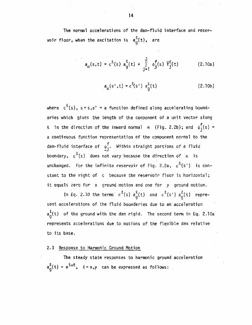
14

The normal accelerations of the dam-fluid interface and reser

voir floor, when the excitation isa~(t), are

(2.1 Oa)

(2.1 Ob)

where e:£(s), s =s,s' = a function defined along accelerating bound

aries which gives the length of the component of a unit vector along

£ in the direction of the inward normal n (Fig. 2.2b); and ¢!(s) =

a continuous function representation of the component normal to the

dam-fluid interface of ¢~. Within straight portions of a fluid-J

boundary, e:£(s) does not vary because the direction of n is

unchanged. For the infinite reservoir of Fig. 2.2a, e:£(SI) is con~

stant to the right of c because the reservoir floor is horizontal;

it equals zero for x ground motion and one for y ground motion.

In Eq. 2.10 the terms e:~(s) a~(t) and e:£(s') a~(t) repre

sent accelerations of the fluid boundaries due to an acceleration

a~(t) of the ground with the dam rigid. The second term in Eq. 2.10a

represents accelerations due to motions of the flexible dam relative

to its base.

2.3 Response to Harmonic Ground Motion

The steady state responses to harmonic ground acceleration

a~(t) = eiwt , £= x,y can be expressed as follows:

15

",Q, 2 -,Q, l' tY•(t ) = -w y, (w) e wJ J

( ) -( ) iwtP x,y,t = P x,y,w e

(2.11)

where the complex frequency response function for a response quantity,

say r(t), is denoted by r(w). Substituting the appropriate terms

of Eq. 2.11 into Eq. 2.5 results in

where

,Q, = x,y (2.12)

(2.13)

Substituting the above expressions for a~(t), Y~(t), and

p(x,y,t) into Eqs. 2.7 to 2.10 leads to the Helmholtz equation:

(2.14)

with the boundary condition along the dam-fluid interface and reser-

voir floor,

16

(2.15)

where

~ 2 J f £a (s,w) = E (s) -w L cf>J'(s) YJ.(w)

n j=l(2.16)

a (s I ,w) = E~ (s I )

n

and the boundary condition at the free surface,

p(x,H ,w) = 0 (2.17)

p(x,y,w) is the solution of Eq. 2.14 subject to the boundary condi

tions of Eqs. 2.15 and 2.17 along with the radiation condition if the

fluid domain is infinite.

Because the governing equation as well as boundary conditions

are linear, using superposition p(x,y,w) can be expressed as

Jp(x,y,w) =p~(x,y,w) - w2 L PJ.(x,y,w) YJ~(w)

j=l(2.18)

-~where po(x,y,w) is the solution of Eq. 2.14 with boundary conditions

Eqs. 2.15 and 2.17 where

~a (s) = E (s),n

s = S,SI (2.19)

Pj(x,y,w) is the solution of Eq. 2.14 with boundary conditions

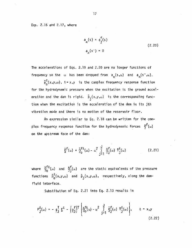
17

Eqs. 2.15 and 2.17, where

a (s) = ep~(s)n. J

a(s')=On.

(2.20)

The accelerations of Eqs. 2.19 and 2.20 are no longer functions of

frequency so the w has been dropped from an.(s,w) and an(s',w).

p~(x,y,w), t= x,y is the complex frequency response function

for the hydrodynamic pressure when the excitation is the ground accel

eration and the dam is rigid. Pj(x,y,w) is the corresponding func

tion when the excitation is the accel~ration of the dam in its jth

vibration mode and there is no motion of the reservoir floor.

An expression similar to Eq. 2.18 can be written for the com

plex frequency response function for the hydrodynamic forces Qf(w)

on the upstream face of the dam:

(2.21)

-ft -fwhere Q (w) and Q.(w)-0 -J

-t(functions Po x,y,w) and

fluid interface.

are the static equivalents of the pressure

Pj(x,y,w), respectively, along the dam-

Substitution of Eq. 2.21 into Eq. 2.13 results in

= - t = x,y

(2.22)

18

Equations 2.12 and 2.22 for j = 1;2, ... ,J can be rearranged and

assembled into matrix form as

-i i~(w) y (w) = ~ (w),

where

i = x,y (2.23)

(2.24)

~(w) is a symmetric matrix and is the same for ~ = x,y components

of ground motion.

Hydrodynamic terms appear on both sides of Eq. 2.23, as added

loads on the right and added masses on the left, the latter also

coupling the modal equations. The added load terms are associated

with hydrodynamic pressures on the dam face due to ground accelera

tions while the dam is rigid. Added mass terms arise from hydrody~

namic pressures due to motions of the dam relative to its base. The

hydrodynamic terms depend on the excitation frequency, a consequence

of the fluid compressibility. For an incompressible fluid C = 00,

and Eq. 2.14 reduces to the Laplace equation; the hydrodynamic terms

become independent of frequency.

2.4 Response to Arbitrary Ground Motions-~The complex frequency response functions Yj(w), j= 1,2, ... ,J

are obtained by solving the set of equations (Eq. 2.23) for a range of

19

values of the excitation frequency w. Solutions corresponding to

i = x and y are Y~(w) and Y~(w), respectively. Responses to anJ. J

arbitrary ground acceleration ai(t) can be obtained from the comg

plex frequency responses by a Fourier synthesis of the responses to

individual harmonic components:

00

y~( t) =_1 f Y~(w) Ai(w) eiwt dw,J 27T J g

_00

where A~(w) is the Fourier transform of a~(t):

i = x,y (2.25)

t d

A~(w) =. f a~( t) e- iwt dt,o

i = x,y (2.26)

and where t d = duration of ground motion. The transforms of

Eqs~; 2.25 and 2.26 are performed on discrete functions using the Fast

Fourier Transform (FFT) algorithm.

The total response Yj(t) to simultaneous horizontal and verti

cal components of ground motion is

= y~(t) + y~(t)J J

(2.27)

The nodal displacements yet) are then obtained using the transforma

tion of Eq. 2.3. At any instant of time, stresses in each finite

20

element can be determined from the nodal displacements by stress

displacement transformation matrices for the finite elements.

2.5 Modifications to Include Fluid-Foundation Interaction

At the boundary of a fluid and a flexible foundation, the

acceleration boundary condition which states proportionality between

the pressure gradient normal to the boundary and the normal component

of acceleration is still valid. However, these accelerations can not

be specified as in the rigid foundation case because they depend on

the interaction between the fluid and the flexible foundation. The

actual accelerations, then, are composed of a free-field part and a

part caused by the interaction. Furthermore, a pressure wave travel

ling in the fluid which strikes a flexible but stationary foundation

produces accelerations at the boundary, but by interaction only since

the free-field accelerations are zero. Such an incident pressure wave

is only partially reflected since a portion refracts into the

founda t ion.

2.5.1 One-dimensional fluid-foundation system

Consider the one-dimensional problem of Fig. 2.3 which consists

of adjoining fluid and foundation half-spaces. This problem is one

dimensional because no variations are present in the x direction.

Harmonically varying pressures in the fluid and displacements in the

foundation are p(y,w) and u(y,w), respectively. The excitation is

provided by an incident displacement wave travelling upward through

the foundation.

Pressures within the fluid obey the one-dimensional version of

Eq. 2.14:

21

~WATER

p(y,W)

yx

FLEXIBLE FOUNDATIONINCIDENT01 SPLACEMENTWAVE

FIG. 2.3 ONE-DIMENSIONAL FLUID-FOUNDATION SYSTEM

22

(2.28)

Taking the fluid-foundation boundary as the y = 0 line, the accel

eration boundary condition for the fluid can be written from Eq. 2.15

as

~ (o,w) =~ w2 u(o,w} (2.29)

Within the foundation displacements are also governed by the one

dimensional Helmholtz equation

2- 2d u w --2+-2 u =0dy C

r

(2.30)

where Cr = compression wave velocity in the foundation. The general

solution to Eq. 2.30 is

. w W1 - Y -i - y

u(y,w) = A(w) e Cr + B(w} e Cr (2.31)

where A(w) is the unknown amplitude of the reflected displacement

wave and B(w) is the specified amplitude of the incident wave. A

free-field acceleration of ay is obtained if

B(w) 1= --a2w2 y

(2.32)

23

Such an upward propagating wave has an acceleration amplitude of

~ ay which doubles to ay upon reflection at a free boundary at

y = o.

A(w) in Eq. 2.31 is evaluated from the condition that the pres-

sure in the fluid at the foundation equals the normal foundation stress

there. Taking compression positive,

(2.33)

where Er == the elastic modulus of the foundation rock given by

and where wr = unit weight of the rock. Substitution of

Eqs. 2.31 and 2.32 into Eq. 2.33 and solution for A(w) yields

(2.34)

A(w) 1 i n - )= - ---2 a + ---~ p(o,w2w y wC r wr

(2.35)

And substitution of Eqs. 2.31, 2.32 and 2.35 into Eq. 2.29 yields a

new form of the fluid boundary condition:

~ (o,w) = - ~ a + iwq p(o,w)g y (2.36)

24

_ wwhere q - w-c-' Terms on the right side of Eq. 2.36 represent por-

r r

tions of the fluid boundary acceleration due to free-field motions and

interaction, respectively. Since the interactive acceleration is pro

portional to ioo ~(o,oo), the derivative of the pressure at y = 0

with respect to time, it can be interpreted as a damper and q as a

damping coefficient. For a rigid foundation, q = 0 in Eq. 2.36,

and ay is an actual, specified acceleration of the fluid boundary.

Equation 2.36 also provides for the proper partial reflections

of a downward travelling pressure wave which strikes the fluid-

foundation boundary. The general solution of Eq. 2.28 is

i ~ y -i ry~(y,oo) = f(oo) e C + 8(00) e (2.37)

where A(oo) is the specified amplitude of the hydrodynamic pressure

wave incident to the reservoir floor, and 8(00) is the amplitude of

the reflected wave. The ratio B(oo)/A(oo), termed the reflection

coefficient ar , can be found by substituting Eq. 2.37 into the

boundary condition Eq. 2.36 with a = 0 (zero free-fieldy

accelerations). Thus,

1 wC-we1 - gC _ r r

a = 1 + qC +~r 1 w Cr r

which is independent of frequency oo. Also,

(2.38a)

1 1q = C 1 (2.38b)

25

2.5.2 Two-dimensional fluid-foundation systems

Equation 2.36, although strictly applicable to one-dimensional

systems, can be applied as the acceleration boundary condition along

the reservoir floors of Fig. 2.1 to approximately account for fluid

foundation interaction. Equation 2.36 is generalized to

*(s',w) = - ~ al1(s') + iwqp(s',w) (2.39)

which replaces the portion of Eq. 2.15 along the reservoir floor.

Equation 2.15 then is a special case of Eq. 2.39 for q =0, the

rigid foundation case. a (51) of Eq. 2.39 is the free-field accel11

eration of the reservoir floor. It is zero for computation of the

pressures Pj(x,y,w) as stated by Eq. 2.20 and usually non-zero for

• -5/,() 1computatlon of the pressures Po x,y,w ,. 5/,= x,y. In the atter case,

the variation of a (Sl) along the floor can approximately be11

defined by Eq. 2.19 with the same function £5/,(5') as used for the

rigid motion.

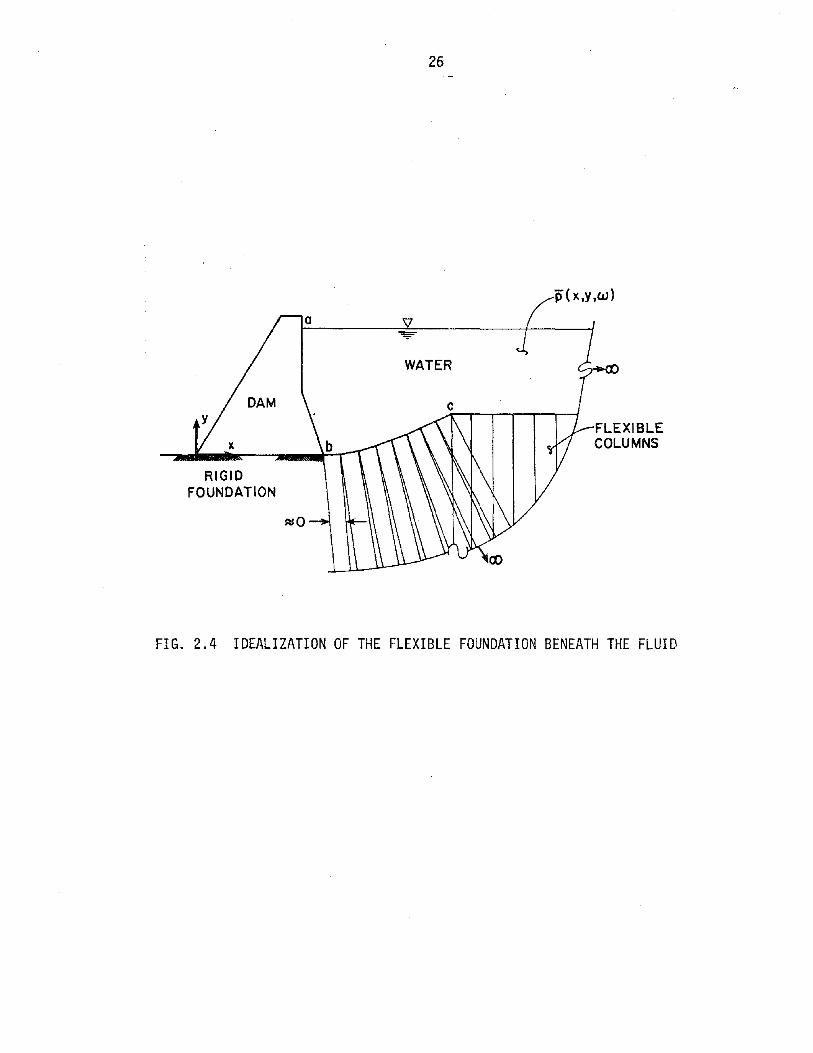
Equation 2.39 can be interpreted as the result of idealizing

the foundation as shown in Fig. 2.4. Portions of the foundation

beneath the fluid are sliced into columns of infinite length and infini-

tesimal width extending in a direction perpendicular to the fluid

boundary. Resulting foundation motions are due entirely to axially

travelling compression waves in the columns, each of which vibrates

independently of its neighbor. Continuity is maintained between nor

mal displacement and stress across the fluid-foundation boundary. The

properties Er , wr ' and Cr are now those of the columns.

26

RIGIDFOUNDATION

WATER

FLEXIBLECOLUMNS

FIG. 2.4 IDEALIZATION OF THE FLEXIBLE FOUNDATION BENEATH THE FLUID

27

Consideration of a single column, an incident wave travelling toward

the fluid domain, and the pressure response p{s',w) at the end of

the column leads to Eq. 2.39 by a derivation similar to that of

Eq. 2.36. an{s') is the free field acceleration at the end of the

column.

The foundation model of Fig. 2.4 and the equivalent formulation

Eq. 2.39 are simplifications of real situations, but they do provide

an additional mechanism for energy loss (radiation through the

foundation) which does exist in real problems and which is not

accounted for by a rigid foundation model. The amount of energy loss

depends on the value chosen for the damping coefficient q.

Magnitudes of Cr and wr used in computing q can be taken as

actual values of the foundation rock or adjusted to improve the per

formance of the sliced column foundation. For example, in Fig. 2.4,

increasing Cr and wr above foundation rock values would approxi

mately cancel the loss in stiffness due to the slicing and the loss in

mass due to the empty spaces between columns. Both adjustments result

in a smaller q and a value of the reflection coefficient ar closer

to one. Should a silt layer overlie the foundation rock, a higher

value of q may be appropriate.

As shown in later chapters, a reasonable value of q affects

the fluid response only locally in the vicinities of frequencies where

the fluid response is very high. The radiation of energy into the

foundation reduces these high (and unrealistic) responses which occur

for the rigid foundation model. Thus, the approximate flexible founda

tion model is a significant improvement.

29

3. TWO-DIMENSIONAL ANALYSIS OF HYDRODYNAMIC FORCE VECTORS

3.1 Boundary Value Problems and Solution Techniques

As seen in Chapter 2, hydrodynamic force vectors of Eq. 2.24-fi fare of two types: added 10adQ (w), i = x,y and added mass Q. (w).-0 -J

These vectors are obtained from hydrodynamic pressure distributions

along the dam-fluid interface which are found by solving the Helmholtz

equation:

(3.1)

subject to the acceleration boundary condition along the dam-fluid

interface

and along the reservoir floor

~ (s' w) = - ~ a (s') + iwq p-(SI,W)an' g n.

the zero pressure condition at the free surface (y = H)

p(x,H,w) = a

(3.2a)

(3.2b)

(3.3)

and the radiation condition if the fluid domain extends to infinity in

the upstream direction. In Eq. 3.2b, values of the damping coefficient


30

q greater than zero are used to approximately account for fluid

foundation interaction effects; in which case, a (s') is the freeYl.

field acceleration of the reservoir floor. For a rigid foundation,

q = O.

9.a (s) = £ (s),Yl.

s = s,s' (3.4)

and the solution to the resulting boundary value problem (B.V.P.) is

the hydrodynamic pressure Po9.(x,y,w). The force vector Qf9.(w) can-0

be obtained from the pressures along the dam-fluid interface by the

method of virtual work. For computation of g!(w) (see Eq. 2.20),

a (s) = cj/(s)Yl. J

a (s') = 0Y/.

(3.5a)

(3.5b)

for each of the J natural modes of vibration of the dam. Pj(x,y,w)

is the solution to the resulting B.V.P. with corresponding force vector

Q!(w).-J

If the fluid domain extends a short distance upstream (Fig. 3.la),

the above B.V.P.'s are solvable with the finite element method. This

technique which can handle arbitrary, but finite, fluid domain geome

tries is described in Sec. 3.2. Should the fluid domain extend a great

distance upstream, then an infinite model is more appropriate. The

31

WATER

(a) FINITE,IRREGULAR GEOMETRY

c

a 'il

WATER

b

(b) INFINITE, CONSTANT DEPTH

WATER

(c) INFINITE, IRREGULAR GEOMETRY

'il d

WATER

o

CONSTANTDEPTH

(d) INFINITE, IDEALIZED IRREGULAR GEOMETRY

FIG. 3.1 FLUID DOMAIN TYPES

32

simplest such case, shown in Fig .. 3.1b, has a vertical dam-fluid inter

face a-b and horizontal reservoir floor. For this fluid domain,

series solutions to the B.V.P.ls have been reported (7) and are out

lined in Appendix E. A combined finite element-continuum solution of

the same problem is presented in Sec. 3.3. Both treatments for the

fluid domain of Fig. 3.1b require that the acceleration of the reser

voir floor not vary along the infinite length of the floor. This

requirement is consistent with the zero acceleration condition of

Eq. 3.5b and also, since the floor is straight, with the ££(Sl) con-

dition of Eq. 3.4.

Figure 3.1c shows a more realistic fluid domain with geometric

irregularities. If this fluid domain is idealized as shown in Fig. 3.1d

with a finite region a-b-c-d-a of irregular geometry coupled to an

infinite region of constant depth to the right of the vertical line

c-d, then the B.V.P.ls can be solved by a method described in Sec. 3.4.

This method utilizes the standard finite element formulation of Sec. 3.2

for the region a-b-c-d-a and the finite element-continuum treatment

of Sec. 3.3 for the infinite region. Accelerations of the horizontal

reservoir floor to the right of c can not vary along the infinite

length, a requirement consistent with Eqs. 3.4 and 3.5b.

The analysis procedures of Sees. 3.2 to 3.4 are for hydrodynamic

pressures and are written for general accelerations rather than the

specific conditions of Eqs. 3.4 and 3.5. These specific conditions are

considered in Sec. 3.5 as is the actual computation of 9b£(w), £= x,y

and g;(w) from the resulting pressures along the dam-fluid interface.

33


Solution of the B.V.P. of Sec. 3.1 (Eq. 3.1 subject to boundary

conditions of Eqs. 3.2 and 3.3) for finite fluid domains of irregular

geometry (Fig. 3.2a) can be obtained numerically by the finite element

method (12). In this approach, the fluid domain is divided into two-

dimensional finite elements as shown in Fig. 3.2b. The interelement

hydrodynamic pressure is defined in terms of discrete values Pi(w)

at the element nodal points. These nodal pressures are the unknowns in

the B.V.P., one OaF for each node below the fluid free surface (where

the nodal pressures are zero) assembled into the vector p(w). A

finite element discretization of the B.V.P. of Eqs. 3.1 to 3.3 leads to

the matrix equation (Appendix B.l):

(3.6)

where ~, ~, and § are symmetric matrices analogous to stiffness,

damping, and mass matrices arising in dynamics of solid continua; and

p = vector of nodal accelerations computed from the normal accelerations

along the dam-fluid interface a-b and a (s') along theY/.

reservoir floor b-c, and thus can have non-zero terms for only nodes

along a-b-c. The non-zero portion of ~ is a submatrix corresponding

to nodes along b-c where the boundary condition of Eq. 3.2b is

applied. Only OaF for nodes below the free surface a-c are included

in Eq. 3.6.

The unknown pressures p(w) can be determined by solving the

set of algebraic equations (Eq. 3.6) simultaneously. For the case

Q

34

iH Il,Y ,Coil)

(a) FLUI D DOMAIN

(b) FINITE ELEMENT DISCRETIZATION

FIG. 3.2 FINITE FLUID DOMAIN OF IRREGULAR GEOMETRY

35

q =0, ~(w) can also be determined using an eigenvector expansion.

The eigenprob1em associated with Eq. 3.6 for q = 0 is

(3.7)

which upon solution yields real valued eigenvalues Ym and eigen

vectors S. The eigenvectors are orthogonal to Hand G and are-mnormalized so that

and they then satisfy

sT G s =1-m - -m(3.8a)

(3.8b)

e(w) is expressed approximately as a linear combination of the

first M eigenvectors:

(3.9)

Substituting Eq. 3.9 into Eq. 3.6 with q = 0, premu1tiplying the

result by ~T, and solving for ~(w) using the orthogonality pro

perty of the eigenvectors results in

(3.10)

where r = an Mx M diagonal matrix with mth diagonal term222= Ym - w Ie. From Eqs. 3.9 and 3.10

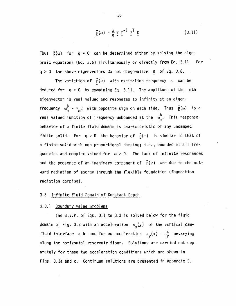
36

(3.11)

Thus E(w) for q = a can be determined either by solving the alge

braic equations (Eq. 3.6) simultaneously or directly from Eq. 3.11. For

q > a the above eigenvectors do not diagonalize ~ of Eq. 3.6.

The variation of p(w) with excitation frequency ttl can be

deduced for q =a by examining Eq. 3.11. The amplitude of the mth

eigenvector is real valued and resonates to infinity at an eigen

frequency wb = y C with opposite sign on each side. Thus p_(w) is am mbreal valued function of frequency unbounded at the wm' This response

behavior of a finite fluid domain is characteristic of any undamped

finite solid. For q > a the behavior of e(w) is similar to that of

a finite solid with non-proportional damping; i.e., bounded at all fre

quencies and complex valued for w > a.The lack of infinite resonances

and the presence of an imaginary component of p(w) are due to the out

ward radiation of energy through the flexible foundation (foundation

radiation damping).

3.3 Infinite Fluid Domain of Constant Depth

arately for these two acceleration conditions which are shown in

Figs. 3.3a and c. Continuum solutions are presented in Appendix E.

QINFINITELAYER

~CX)

NODALa I ~ ..~ ...I ~

7

b~=-'--

~QX _

~(X)

H

j5 (x,Y,w)

y

b x

ax(y) ,...----.,

(a) ACCELERATION OF DAM-FLUIDINTERFACE

(b) LAYER DISCRETIZATIONOF FIG. a

a a~NODE w

.......

j5 (x,y,w) H

~CO

l+--FINITEELEMENT

y

b x

O(X)=Oiy y

(c) ACCELERATION OF RESERVOIRFLOOR

_b

t~(d) FINITE ELEMENT

DISCRETIZATIONOF FIG. C

FIG. 3.3 INFINITE FLUI D DOMAIN OF CONSTANT DEPTH

38

The governing Eq. 3.1 with the boundary conditions

*(O,y,w) =

~ (x,O,w) =

- ~ a (y)g x

iwq p(x,O,w)

(3.12a)

(3.12b)

p(x,H,w) = ° (3.12c)

defines the first B.V.P. Equation 3.1 with the boundary conditions

~ ( ) -ax O,y,w - ° (3.13a)

~ )ay (x,O,w = w .<. -( )- 9 ay + iwq p x,O,w (3. 13b)

p(x,H,w) = °

defines the second B.V.P.

3.3.2 First B.V.P.

(3.13c)

The simple geometry of the infinite fluid domain of constant

depth permits a separation of variables in Eq. 3.1:

(3.14)

where px(x,w) must satisfy

39

d2Px 2 --;r--K p =0dx'" x

and p (y,w) must satisfyy

2-d P 2-1:-+1. P =0dy Y

where k is a separation constant; and

(3.15a)

(3. 15b)

(3.16)

Boundary conditions include Eq. 3.12a and the separated conditions

dpydy (O,w) = iwq Py(O,w) (3.lla)

(3. 17b)

The one-dimensional Eq. 3.l5b with boundary conditions of Eq.

3.17 defines an eigenvalue problem. A finite element discretization of

the eigenprob1em using a one-dimensional mesh (Fig. 3.3d) leads to the

matrix equation:

(3.18)

40

whose derivation follows from that in Appendix B.2, and where the

matrices ~, ~-i. and rf are symmetric. The non-zero portion of B,(.

is one diagonal term corresponding to the node at b. Only DOF for

nodes below the zero pressure node at a are included in Eq. 3.18.

The eigenvalues An and eigenvectors Pn determined from

Eq. 3.18 are complex valued and dependent on the excitation frequency

w unless q =0; in which case, they are real valued and frequency

independent. The Pn are orthogonal and are normalized so that

and they then satisfy

T .Pn ~ '.1!n = 1 (3.19a)

WT [0- + iwq B-i.J w. = A2 (3. 19b)-n - - - n n

The separated function for the y coordinate, Py(y,w) from Eq. 3.15b,

is expressed in discrete form as

n=1,2, ... (3.20)

Discretization in the x direction is inappropriate because the

fluid domain extends to infinity in that direction. Therefore, con-

tinuum solutions to Eq. 3.15a are employed. The K in Eq. 3.16 can

take on only the values given by

41

(3.21)

Since the infinite fluid domain is excited at x = 0, p (x,w) mustxdecay with increasing. x or travel from x = ° to x = 00. Thus, it

is of the form

n=1,2, ... (3.22)

where the root with both ~n and vn positive is taken in computing

Kn from Eq. 3.21. Including the first N terms in Ey and px

leads to an approximate expression for E(x,w):

e(x,w) (3.23)

where ~(x) = an Nx N diagonal matrix with nth diagonal term-K x

= ell. If q = 0, then An is real; and Kn is real or imaginary

depending on whether w is less than or greater than AnC; i.e.,

Kn = ~n' or Kn = ivn·

The above formulation can be interpreted as a discretization of

the fluid domain into layers of infinite length (Fig. 3.3b) separated

by nodal lines. The ith term of the vector e(x,w) in Eq. 3.23

represents the variation of pressure with x along the ith nodal

line. The nn(w} are determined to satisfy the discrete form of the

boundary condition Eq. 3.12a (Appendix C.l):

42

{3.24}

where cf is the same matrix as in Eq. 3.18; and QX = a vector of

nodal accelerations corresponding to the acceleration ax{Y} of the

darn-fluid interface.

Substituting Eq. 3.23 into Eq. 3.24 results in

{3.25}

where ~ = an Nx N ·di agona1 matri x wi th nth di agona1 term = Kn .

Premultiplication of Eq. 3.25 by !T and solution for ~(w) using the

orthogonality property of the eigenvectors leads to

Substitution of Eq. 3.26 back into Eq. 3.23 results in

- w } -1 T xe(x,w) = g ! ~(x ~ ~ D

At x = 0, Eq. 3.27 reduces to

(3.26)

(3.27)

{3.28}

43

For q =0, An and ~n are real valued. Then from Eq. 3.27,

the amplitude of ~n decays exponentially with increasing x at-~ x -iv x

e n (when w< AnC) or is a nondecayi ng harmoni c e n (when

W>AnC). At an eigenfrequency w~ = AnC, Kn = 0 and the amplitude

of ~n is infinite. The part of the amplitude that approaches infin

ity is real below w~ and imaginary above. Thus, p(x,w) is real for

W< w~' complex for W> wt, and unbounded at frequencies w~. The

harmonic, nondecaying distribution with x in the amplitude of an

eigenvector ~ for w > w~ represents a radiation of energy in the_n n

infinite, upstream direction of the fluid domain. This fluid radiation

damping is non-zero for w > wt and is responsible for the imaginary

component of p(x,w). It does not, however, prevent the infinite

resonances at frequencies w~ above wt because of the orthogonality

of the eigenvectors; i.e., a resonating eigenvector ~n is orthogonal

q > 0,-ivnx

e ,the complex eigenvector ~. has an x distribution of_n

an exponentially decaying harmonic. Thus, all energy is eventually

to the fluid radiation damping which is associated with the lower

eigenvectors. The w~ approximate the eigenfrequencies w~ =

(2n-l)TIC/2H' for the continuum fluid domain (Appendix E). For-).lnX

e

radiated by the foundation. Since this foundation radiation damping

occurs for all frequencies greater than zero, p(x,w) is bounded at

all frequencies and complex valued for w > O.

3.3.3 Second B.V.P.

The B.V.P. of Eq. 3.1 with the boundary conditions of Eq. 3.13

contains no variation in the x direction, and is thus one-dimensional

in the y coordinate. Omitting the x variations from these equations

44

results in the one-dimensional Helmholtz equation for p(y,w)

2- 2<L~+~p=Oif C

2

and the boundary conditions

(3.29)

$- (O,w) = (3.30a)

p(H,w) = 0 (3.30b)

Solution of Eq. 3.29 subject to the boundary conditions of

Eq. 3.30 can be obtained by the finite element method using a one

dimensional mesh (Fig. 3.3d). The finite element discretization of the

one-dimensional B.V.P. is the matrix equation (Appendix B.2):

(3.31)

where ~, B~ and ~ are the same symmetric matrices as in Eq. 3.18;

E(w) = vector of unknown nodal pressures; and gi = vector of nodal

accelerations (a zero vector except the term corresponding to the node

at b, whose value is a~). Only DOF for nodes below the zero pres-y

sure node at a are included in Eq, 3.31.

The pressures e(w) can be obtained by solving the algebraic

equations CEq. 3.31} simultaneously. Alternatively, e(w) can be

determined using an eigenvector expansion, employing the complex valued

45

and fre~uency dependent eigenvalues A and eigenvectors ~ resu1t-n -ning from the associated eigenprob1em, Eq. 3.18. Except for q = 0

when both An and ~n are real valued and frequency independent, the

eigencoordinate solution of Eq. 3.31 is inefficient compared to solv-

ing the equations simultaneously. However, if the first B.V.P. is

being solved concurrently, then the frequency dependent An and ~n

are available. Following Eqs. 3.9 to 3.11, e(w) is approximately

expressed in terms of the first N eigenvectors as

p_(w) = ~ ~ A- 1 ~T D~g - -

(3.32)

where! = [~1'~2""'~N] and!: = an Nx N diagonal matrix with nth

diagonal term = A2 - w2/C2. Thus, E(w) can be determined either byn

solving the set of equations 3.31 simultaneously or from Eq. 3.32.

Note that A is related to ~ from Eq. 3.27 by

(3.33)

The frequency variation of e(w) is similar to that of the

finite fluid domain of Sec. 3.2. For q = 0, E(w) is a real valued

function of frequency with infinite resonances at the eigenfrequencies

w~ = AnC (same as the first B.V.P.). For q > 0, E(w) is bounded

at all frequencies and complex valued for w > 0, which are conse-

quences of foundation radiation damping.

46

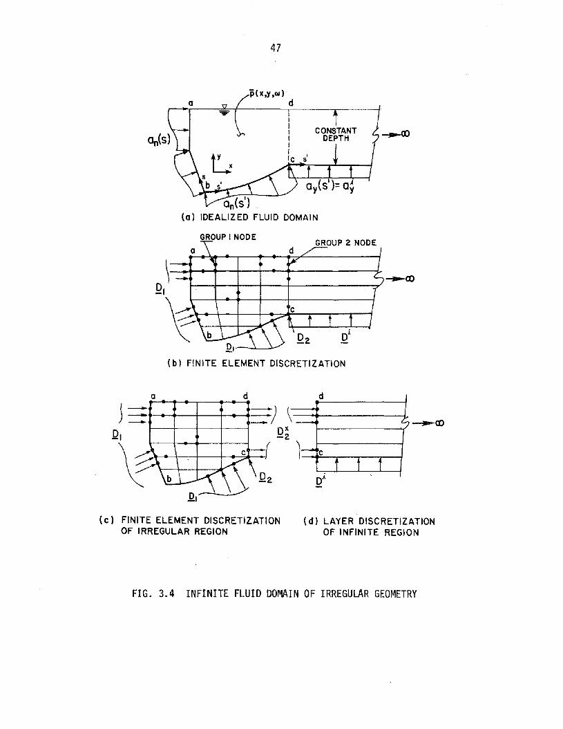
3.4 Infinite Fluid Oomains of Irregular Geortletry

A solution scheme for the B.V.P. of Eqs. 3.1 to 3.3 is pre

sented below for the fluid domain of Fig. 3.4a where a finite region

a-b-c-d-a of irregular shape is connected to an infinite region of

constant depth to the right of the vertical line c-d. Normal accel-

erations of the dam-fluid interface a-b and reservoir floor are

a (s) and a (5'), respectively. To the right of c, a (Sl) = a~,n n n y

unvarying along the infinite length of the horizontal floor. The

fluid domain is discretized as shown in Fig. 3.4b. The finite region

a-b-c-d-a is divided into two-dimensional finite elements as dis-

cussed in Sec. 3.2. Within the infinite region, the layer discretiza

tion of Sec. 3.3 is employed, matching the adjacent two-dimensional

mesh along c-d.

Figures 3.4c and d show the discretized fluid domain separated

at c-d. The separated fluid domains, analogous to free bodies of

solid continua, require that the normal accelerations along the line

of separation be preserved. The finite element matrix equation 3.6 is

written for the region a-b-c-d-a including only OOF for nodes below

the free surface and is partitioned as follows:

[[~~~ ~~~] +iwq [:~~ :~~] - ~~ [,,~~-~+-=-~~:...=..~]] It::;1= ~ IQ2-Q~(W) 1(3.34)

where nodes along c-d are identified by subscript 2 and remaining

nodes by subscript 1. In Eq. 3.34 Ql and Q2 are acceleration

47

iH x,y ,w)do

on(SI)(0) IDEALIZED FLUID DOMAIN

GROUP I NODE

oGROUP 2 NODE

o d d

~(O~-----..."

(c) FINITE ELEMENT DISCRETIZATIONOF IRREGULAR REGION

(d) LAYER DISCRETIZATIONOF INFINITE REGION

FIG. 3.4 INFINITE FLUID DOMAIN OF IRREGULAR GEOMETRY

48

vectors of group 1 and group 2 nodes computed from a (s), s =s,s IYL

along a-b-c; and Q~(w) = acceleration vector of group 2 nodes asso-

ciated with the unknown x-direction acceleration of the line c-d.

Equation 3.34 WithoutQ~(w) is justa partitioned form of Eq. 3.6

written for a zero acceleration condition normal to c-d. However, as

part of the infinite fluid domain of Fig. 3.4a, c-d is an interface

between two subregions and undergoes, as yet, unknown accelerations

which contribute the vector Q~(w) in Eq. 3.34.

Consideration of the infinite region of Fig. 3.4d leads to an

The vector E2(w) of nodal pressures along

the unknown acceleration Q~(w) and

of the floor of the infinite section.

express ion for Q~(w).,

c-d arises from two sources:

the vertical acceleration a~yPressures at c-d due to Q~(w) and a~ are given by Eqs. 3.28 and

3.32, respectively. Using superposition, e2(w) can be expressed as

(3.35)

where use has been made of Eq. 3.33.

If e2(w) is expressed by an eigenvector expansion using the

first N eigenvectors ~-n

(3.36)

then, from Eq. 3.35,

(3.37)

49

Multiplication of Eq. 3.37 by K yields the expression for Q~(w):

(3.38)

Substitution of Eqs. 3.36 and 3.38 into Eq. 3.34 with a premultiplica

tion of the second submatrix equation by ~T yields

El (w)

=

(3.39)

The pressure vector ~l (w) can be obtained by solving the algebraic

equations (Eq. 3.39).

For q = O. several features of the frequency variation of

el(w) are evident. When the frequency is below the first eigen

frequency wt of the infinite region. no imaginary terms are present

in Eq. 3.39. so el(w) is real v~lued. Above wt. El(w) is complex

valued due to fluid radiation damping. Also. when a~ is non-zero,

p,(w) becomes unbounded at each w~ because of the infinite value- nattained by the nth diagonal term of the matrix (1 on the right

side of Eq. 3.39. However, none of the frequencies wi are eigen-. n

frequencies of the complete fluid domain; the infinite responses are

due to the infinite right side of Eq. 3.39 at these frequencies.

50

Eigenfrequencies of the complete fluid domain must satisfy the eigen

value problem associated with Eq. 3.39, this equation with q = 0 and

a zero right side, and be real valued. Such frequencies, if they. .

occur, will be less than w~ because above w~ the eigenproblem is

complex valued (complex matrix ~). At an excitation frequency equal

to an eigenfrequency, El(w) is unbounded if the right side of

Eq. 3.39 is non-zero and if q = O. For q > 0, El(w) is bounded at

all frequencies and complex valued for w > o.

3.5 Computation of Hydrodynamic Force Vectors

For the fluid domains described in Sees. 3.2 to 3.4, computa

tion of the hydrodynamic force vectors ~~$I,(w), $I,=x,y and ~~(w) of

Eq. 2.24 proceeds as follows:

1. The boundary accelerations of Eqs. 3.4 and 3.5 are con

verted into acceleration vectors for use in Eqs. 3.6 or 3.11 (finite

fluid domain), Eqs. 3.28 and 3.32 (infinite fluid domain of constant

depth), or Eq. 3.39 (infinite fluid domain of irregular geometry).

For the finite fluid domain, these vectors are denoted by Q~ and

D., and their computation is described in Appendix 0.1. Use is made-Jof the boundary portion of the finite element mesh along a-b-c in

Fig. 3.2. Vectors {Dx}$I" $1,= x and {Ox}. of Eq. 3.28 and {Dl}$I"- 0 - J - 0

{D2

}Q., Q.=x,y and {Dl }., {D2}. of Eq. 3.39 are computed using the- 0 - J - J

boundary element meshes along a-b in Fig. 3.3 and a-b-c in Fig. 3.4,

respectively, using the method of Appendix 0.1. In the latter case,

{D2}. = O. {tf}Q., Q.=y in Eqs. 3.32 and 3.39 is computed with

- J - - 0

a,t = 1, and {If}\ $I, = x and {If}. of Eq. 3.39 are also zeroy - 0 - J

vectors.

51

2. Using the acceleration vectors of step 1, hydrodynamic

pressure vectors for a fluid domain are obtained by solving the appro

priate equations of Sec. 3.2, 3.3, or 3.4. Pressures along the dam

fluid interface are assembled into pf£(w), £= x,y and p~(w).-0 -J

3. As also described in Appendix 0.1, the hydrodynamic force

vectors are computed from the pressures along the dam-fluid interface

obtained in step 2.

3.6 Numerical Results

3.6.1 Infinite fluid domain of constant depth

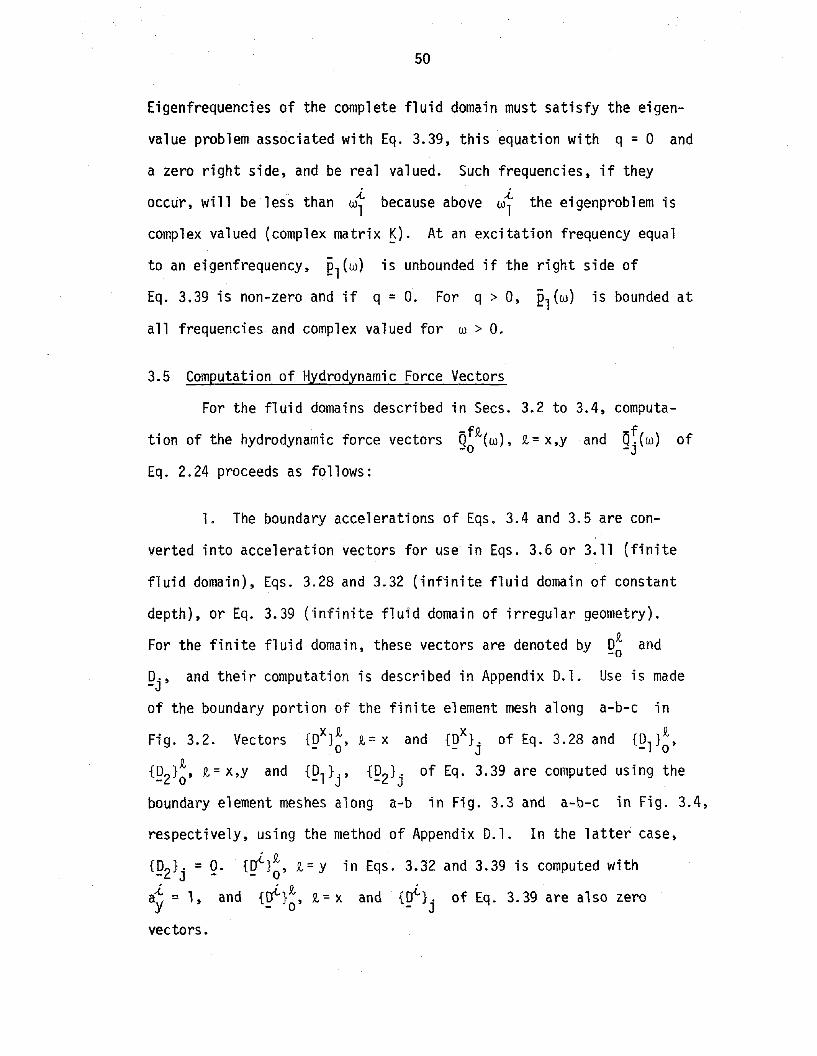
The accelerations shown in Figs. 3.5a and 3.5b result from har

monic ground accelerations = eiwt in horizontal and vertical direc-

tions, respectively, with the dam and foundation assumed rigid.

Continuum solutions to both these problems appear in Appendix E, and

finite element-continuum formulations are discussed in Sec. 3.3. In

order to demonstrate Eq. 3.39 (q=O), these problems are solved here

using regular finite element meshes consisting of single columns of

elements with maximum numbers of eigenvectors included in ~. Three

meshes are used employing 3, 6, and 12 linear elements (Fig. 3.5c) to

demonstrate convergence as the mesh is refined. Two types of plots

are presented: the hydrodynamic force F~(w), £= x,y on the rigid

dam vs. frequency wand the hydrodynamic pressure p~~(Y,w) along

the dam-fluid.interface a-b. F~(w). is computed by integrating-f£( -£Po y,w) over a-b. Fo(w) is normalized with the static force

Fst = lw H2, w with w~ = rrC/2H, and p~£(y,w) with the static

pressure at the reservoir floor wH, so that the results apply to

a a

ax(y)=1y

p~(x,y,(II)

ji~(x ,y, (II)

H

~CX)

b x b x

(a) HORIZONTAL GROUNDMOTION aj = Iy

(b) VERTICAL GROUND MOTION

(J1

N

~CX)

.a

-+l k-H/12

-

-

b

('J

.....:I:

@('J

~CX)

.a-

l

b

II).....:I:

@,II)

I~~

(c) FINITE ELEMENT MESHES

---co

l"H/3"

a

l

bI~ _I

10.....:I:

@,10

FIG. 3.5 INFINITE FLUID DOMAIN OF CONSTANT DEPTH SUBJECTEDTO HARMONIC GROUND MOTIONS WITH RIGID DAM

53

fluid domains of any height. Continuum solutions obtained from the

equations of Appendix E appear as solid lines in the figures.

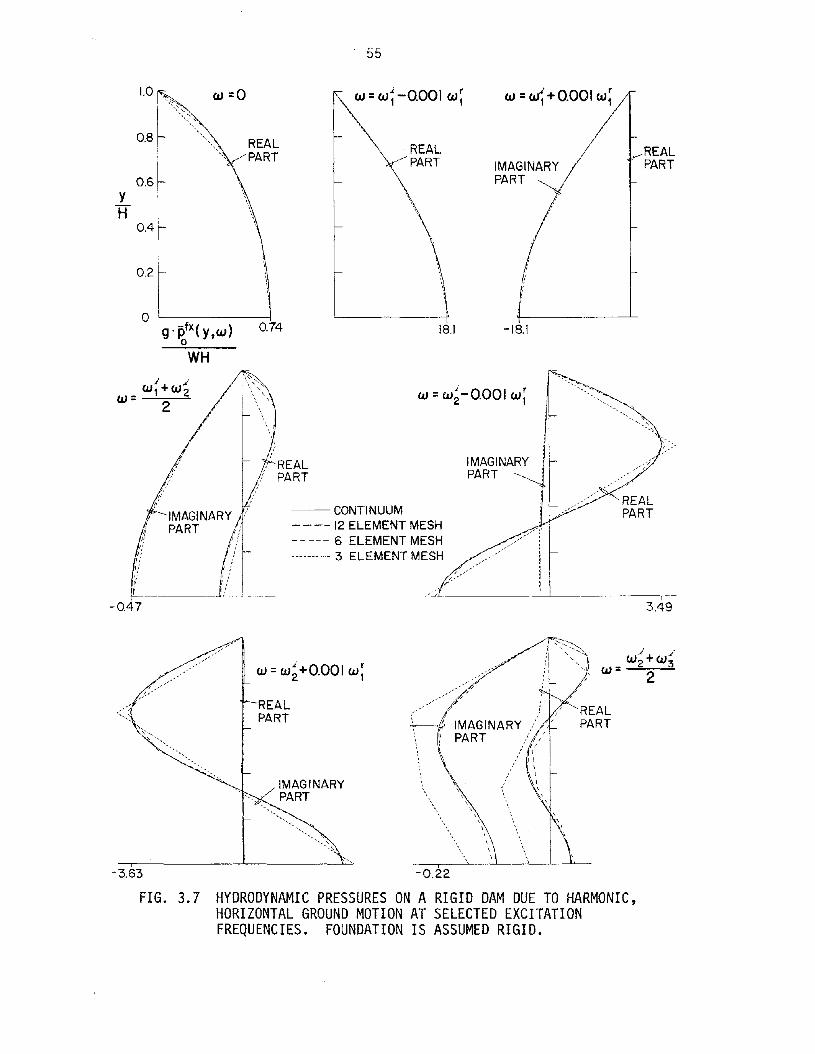
Hydrodynamic forces and pressures due to horizontal ground

motion (Fig. 3.5a) are plotted in Figs. 3.6 and 3.7, respectively.

In the force plot of Fig. 3.6, the location of resonant peaks of the

finite element curves, the eigenfrequencies w~, are shifted toward

higher w. This shift is due to the discretization and is noticeably

less for the finer meshes. The method of resonance, real on the left

and imaginary on the right of the eigenfrequencies, is truely repro

duced by all three finite element solutions. Convergence of these

solutions to the continuum solutions as the mesh is refined is evident

in Fig. 3.6 and also in the pressure plots of Fig. 3.7. There, win

denotes either wr of the continuum results or wi of the finiten n

element results.

For the vertical ground motion case of Fig. 3.5h, hydrodynamic

forces and pressures are plotted in Figs. 3.8 and 3.9, and conclusions

similar to those above can be made. Here, the method of resonance

differs, always real but of opposite sign across the w~ (typical ofn

finite fluid domains), and is truely reproduced by all three meshes.

The effect on the frequency variation of F~(w} of including

less than the maximum number of eigenvectors in ~ is illustrated in

Figs. 3.l0a and b for horizontal and vertical ground motions,

respectively. The three curves plotted are for the six element mesh

with six, two, or one eigenvectors included in ~. The single eigen-

vector solution is satisfactory to just past the first resonant peak,

and the two eigenvector solution is satisfactory to just past the

second peak. Examination of the pressures (not shown) supports these

54

II :I -- CONTINUUM2 --- 12 ELEMENT MESH3 ----- 6 ELEMENT MESH4 --------- 3 ELEMENT MESH

IIIIIIIIIIIII

--+-:-:-~-r-:_- __

I

I!:i!:

I nI"

.......... - .... ,11_ \ J ............ --__

t---1-'> 1,2,3,4

I.

2.

6.

IIIII II IJ_ ~

5.4.3.

I1II

I 'II ,

I 'I ,

I 'I 'II

I 'I

I :I •

I

I :I

I '1 ,I ,II ,

I 'I ,

f ,

~~_ ..,'

1,2,3,4

I. 2.

I.

°O~-~-----!-----!---_...L--_--.JL-_---L6.

2.

1,2,3,4

0'I ---------------

°O!:----L---!:----~--L....--L....--L....-3. 4. 5. 6.W/W

rI

FIG. 3.6 HYDRODYNAMIC FORCE ONA RIGID DAM DUE TO HARMONIC,HORIZONTAL GROUND MOTION. FOUNDATION IS ASSUMED RIGID.

55

I

3.49

REALPART

REALPART

w =w~+0.001 w~

IMAGINARYPART

IMAGINARYPART

I

18.1 -18.1

. REALPART

w =w~ -0.001 w~

----12 ELEMENT MESH .,: ~----- 6 ELEMENT MESH ..,/ i---------- 3 ELEMENT MESH ../...... i"

~:;;;r i !/" .

-- CONTINUUM

REALPART

1.0'" w=o",*"~,

" ,",'"

0.8 REALPART

0.6YH

0.4

0.2

0g' j)fx( y w) 0.74

o t

WH"i .,to

w=W 1+W 2

2

-3.63

".

".

w=w~+O.OOI w;REALPART

IMAGINARYPART

-0.22

REALPART

FIG. 3.7 HYDRODYNAMIC PRESSURES ON A RIGID DAM DUE TO HARMONIC,HORIZONTAL GROUND MOTION AT SELECTED EXCITATIONFREQUENCIES. FOUNDATION IS ASSUMED RIGID.

56

6.

!'.,'.'.'."'."'.'."'.'.'.'.'.""'."'.'."'.'.""'.'.'.'.'.'.'.'."'.""'.'.·.·.·.· .· ,· .

I ~""

5.4.

I.

I -- CONTINUUM2 ----12 ELEMENT MESH3 ----- 6 ELEMENT MESH4 ---------- 3 ELEMENT MESH

2.

-2·0~---'---'----'---_...llJ--"---_---L-__-'-J.---'------'--

I. 2. 3. 4. 5. 6.r

W/W 1

00 I. 2. 3.

2.

1,2,3,4

I.

-:3- ->.~ 0II.L.°

CI

-I.

FIG. 3.8 HYDRODYNAMIC FORCE ON A RIGID DAM DUE TO HARMONIC,VERTICAL GROUND MOTION. FOUNDATION IS ASSUMED RIGID.

57

406. - 405.

w =W1 +0.001 W~w =w~-o.OOI W~

t~--------t'

1.0 w=O

0.8

0.6Y IH

0.4

0.2

0g' p;Y(y,W) I.

WH

w =w~-o.OOI W~

/( ,-- ,-'.

--CONTINUUM----12 ELEMENT MESH----- 6 ELEMENT MESH---------- 3 ELEMENT MESH

-0.32 135.

w =w~+o.OOI W~

I135. 0.16

FIG. 3.9 HYDRODYNAMIC PRESSURES ON A RIGID DAM DUE TO HARMONIC,VERTICAL GROUND MOTION AT SELECTED EXCITATIONFREQUENCIES. FOUNDATION IS ASSUMED RIGID.

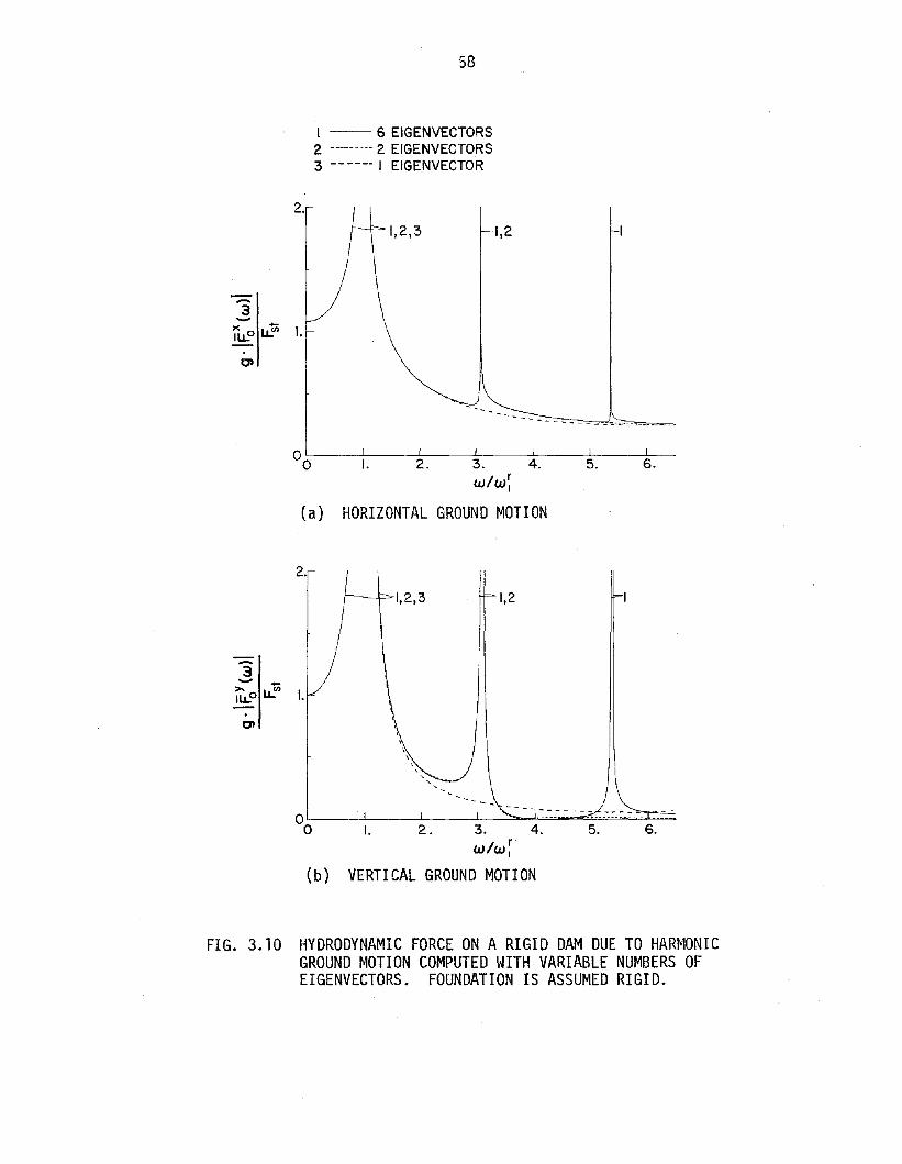
58

I -- 6 EIGENVECTORS2 --------- 2 EiGENVECTORS3 ------ 1 EIGENVECTOR

2.

-:3-x -IIJ..0 IJ..(/) i.

1,2,3 1,2

(a) HORIZONTAL GROUND MOTION

2.

r-----_'_==> I, 2 ,3 I,2

,,,\

\\

\ , ,

I. 2. 3. 4.W/W r

I

5. 6.


FIG. 3.10 HYDRODYNAMIC FORCE ON A RIGID DAM DUE TO HARMONICGROUND MOTION COMPUTED WITH VARIABLE NUMBERS OFEIGENVECTORS. FOUNDATION IS ASSUMED RIGID.

59

observations. Thus, the number of eigenvectors included in an ana1y-

sis can be less than the maximum and depends on the range of excitation

frequency required. The shape of the acceleration distribution is

another factor; non-uniform accelerations tend to excite higher eigen

vectors so more need be included.

The problems of Figs. 3.5a and b are also solved with damping

incorporated into the acceleration boundary condition along the reser

voir floor to approximately account for fluid-foundation interaction

as discussed in Sec. 2.5. a~ is now a free-field acceleration, andy

the reflection coefficient a is chosen as .85. F~(w) vs. w curvesr 0

are presented in Figs. 3.11 and 3.12 for horizontal and vertical

ground motions, respectively. Continuum solutions are from Appendix E,

while the finite element results were obtained with Eq. 3.39 and the

twelve element mesh of Fig. 3.5c with all twelve eigenvectors included

in ~. Agreement between the curves is comparable to that obtained

for the corresponding curves of Figs. 3.6 and 3.8 for the rigid fluid

foundation. Note that responses accounting for fluid-foundation inter

action are bounded functions of excitation frequency wand complex

valued for w > O. For the horizontal ground motion case (Fig. 3.11),

finite real and imaginary peaks replace the infinite real and imaginary

responses of Fig. 3.6. And for vertical ground motion (Fig. 3.12),

finite real peaks replace the infinite real responses of Fig. 3.8, and

new imaginary peaks appear centrally located over the w~. The behavn

ior for vertical ground motion is typical of that for finite fluid

domains.

60

4.

3.I CONTINUUM2 ------FINITE ELEMENT

1,2

I.

°O~-------,---~--------,~_---L__----l-__l...--5. 6.

4.

.-.. 3.3'-)(IIJ..°- - 2.IJ..IIl

Ce 1,2

CI

I.

.-.. 3.-~)(

IIJ..°-CI 1J..1ii 2.0E

CII I.

I. 2. 3. 4. 5. 6.

FIG. 3.11 HYDRODYNAMIC FORCE ON A RIGID DAM DUE TOHARMONIC, HORIZONTAL GROUND MOTION.FLUID-FOUNDATION INTERACTION IS INCLUDED.

61

12.

10.

8.

I CONTINUUM2 ------ FINITE ELEMENT

-3~ ~ 6.ILLo u.:

1,2

C' 4.

2.

o0~-~1.--==2~.==~3~.~-.L.-._....a:::~_J.--4. 5. 6.

6.

1,2

2.

4.

-3>.ILLo-..- -

o LL..'" 0 r----t--======-p----.-L--~=--..!.-.-Q)'-

C' -2.

-4.

6.5.I.-6.'--_~__-L.-__l.___ _____.l___.L__..L___

o10.

8.

~ 1,2->. 6.ILLo-..-

g'u? 4.E

'i" 2.

-2b~-----L---L.---l.--------.l---.L--..L---2. 3. 4. 5. 6.

W/WrI

FIG. 3.12 HYDRODYNAMIC FORCE ON A RIGID DAM DUE TOHARMONIC, VERTICAL GROUND MOTION.FLUID-FOUNDATION INTERACTION IS INCLUDED.

62

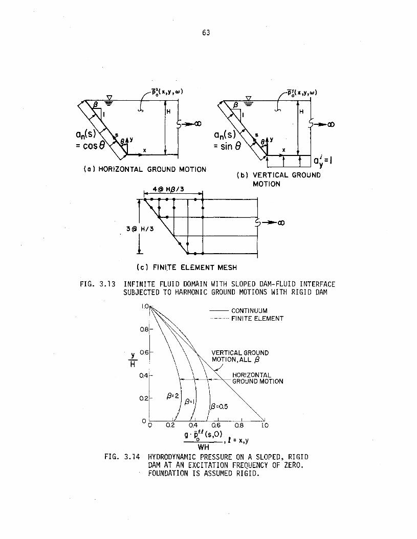
3.6.2 Infinite fluid domain with sloped dam-fluid interface

As shown in Fig. 3.13 the dam-fluid interface slopes outward at

slope 8:1; the depth of the fluid domain is constant beyond the toe

of the dam. The accelerations in Figs. 3.13a and b result from har

monic ground accelerations = eiwt in horizontal and vertical direc-

tions, respectively, with the dam and foundation assumed rigid. For

an excitation frequency of zero, the incompressible water case, inde-

pendent solutions to the problems of Figs. 3.13a and b exist and can

be compared with finite element results from Eq. 3.39. For the hori

zontal motion case of Fig. 3.13a, Fig. 3.14 shows the pressure distri

bution p~x(s,O) along the dam face, normalized with wH, for

8 = .5, 1, 2. Solid lines are an integral equation solution obtained

by conformal mapping techniques (13). Results from Eq. 3.39 (q= 0)

using the mesh of Fig. 3.l3c with all six etgenvectors are also shown.

Agreement is close. Pressures due to vertical ground motion

(Fig. 3.13b) vary linearly with depth and are independent of 8. The

finite element analysis leads to exact results (Fig. 3.14).

63

H

0 1 =1L..---I..----J'---' Y

(b) VERTICAL GROUNDMOTION

H

p~( It,Y, w)

T3@ H/3

1


(c) FINITE ELEMENT MESH

FIG. 3.13 INFINITE FLUID DOMAIN WITH SLOPED DAM-FLUID INTERFACESUBJECTED TO HARMONIC GROUND MOTIONS WITH RIGID DAM

-- CONTINUUM----- FINITE ELEMENT

VERTICAL GROUNDMOTION,ALL f3

HORIZONTALI---t----+....--~ GROUN D MOTION

0.8

0.4

0.2

y 0.6

H

o 0 0.4 0.6 0.8

g' pO (s,O)o ,1= x,yWH

FIG. 3.14 HYDRODYNAMIC PRESSURE ON A SLOPED, RIGIDDAM AT AN EXCITATION FREQUENCY OF ZERO.FOUNDATION IS ASSUMED RIGID.

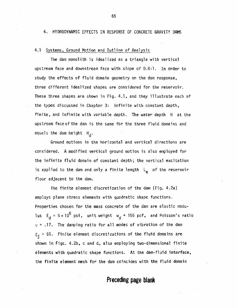
65

4. HYDRODYNAMIC EFFECTS IN RESPONSE OF CONCRETE GRAVITY DAMS

4.1 Systems, Ground Motion and Outline of Analysis

The dam monolith is idealized as a triangle with vertical

upstream face and downstream face with slope of 0.8:1. In order to

study the effects of fluid domain geometry on the dam response,

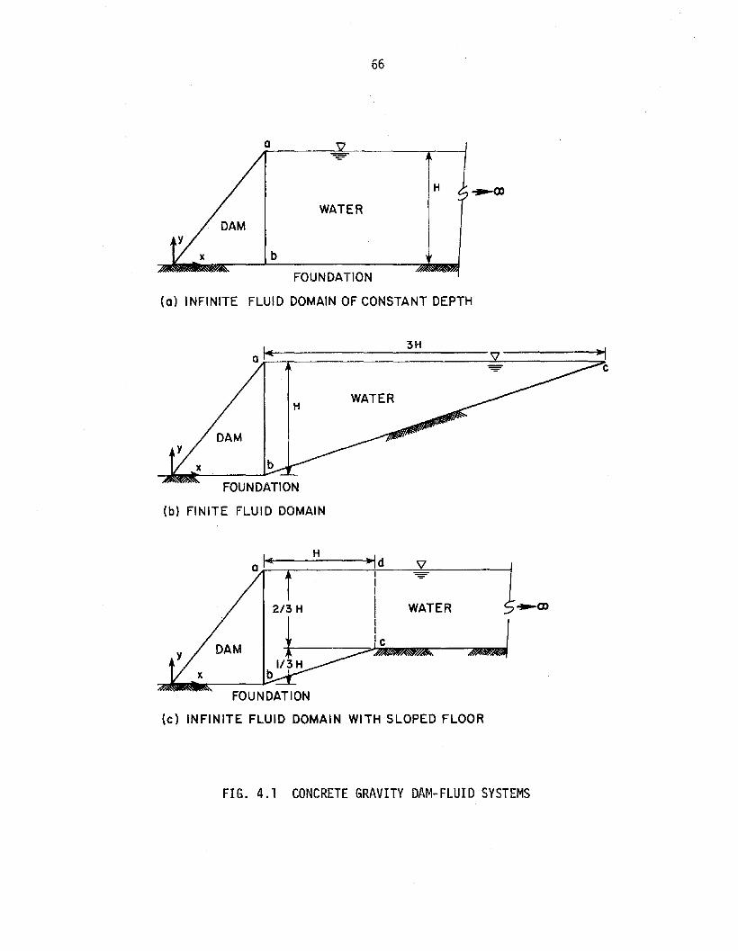
three different idealized shapes are considered for the reservoir.

These three shapes are shown in Fi g. 4.1, and they illustrate each of

the types discussed in Chapter 3: infinite with constant depth,

finite, and infinite with variable depth. The water depth H at the

ups tream face of the dam is the same for the three fl ui d doma ins and

equals the dam height Hd.

Ground motions in the horizontal and vertical directions are

considered. A modified vertical ground motion is also employed for

the infinite fluid domain of constant depth; the vertical excitation

is applied to the dam and only a finite length Le of the reservoir

floor adjacent to the dam.

The finite element discretization of the dam (Fig. 4.2a)

employs plane stress elements with quadratic shape functions.

Properties chosen for the mass concrete of the dam are elastic modu

lus Ed = 5x 106 psi, unit weight wd = 155 pcf, and Poisson's ratio

v = .17. The damping ratio for all modes of vibration of the dam

~j = 5%. Finite element discretizations of the fluid domains are

shown in Figs. 4.2b, cand d, also employing two-dimensional finite

elements with quadratic shape functions. At the dam-fluid interface,

the finite element mesh for the darn coincides with the fluid domain


66

H

WATER

b

FOUNDATION

(a) INFINITE FLUID DOMAIN OF CONSTANT DEPTH

H

FOUNDATION

(b) FINITE FLUID DOMAIN

WATER

3H

e

WATER

H

IIII

2/3 H I

4IIIe

~~~1/3H

b

FOUNDATION

(e) INFINITE FLUID DOMAIN WITH SLOPED FLOOR

FIG. 4.1 CONCRETE GRAVITY DAM-FLUID SYSTEMS

67

a o d

(

b c

I@ H/6 FOR Le =3@ H/3 FOR Le =

-

ex>H

6@ H/3 FOR Le-2H

(b) INFINITE FLUID DOMAINOF CONSTANT DEPTH

~---::--c=-::-c:-:-:-:-~b6 @2H/15

(0) DAM

6@ H/20141( .,

c

ID.......J:

@,\0

(c) FINITE FLUID DOMAIN

b

4@H/4a d

~

~c

[....--"'"

-b

(d) INFINITE FLUID DOMAIN WITH SLOPED FLOOR

FIG. 4.2 FINITE ELEMENT MESHES

68

meshes. The water has unit weight w = 62.4 pcf and compression wave

velocity C = 4720 ft/see. The foundation unit weight wr and compres

sion wave velocity Cr are chosen so that the reflection coefficient

ar computed fro~ Eq. 2.38a equals .85. The damping coefficient q

along the reservoir floor is then given by Eq. 2.38b.

Responses of the dam-fluid system to harmonic ground motions

were computed by the procedure of Chapters 2and 3. The vectors Q~ (w)-J

and §~£(w) of Eq. 2.24 were obtained as described in Sec. 3.5 from

hydrodynamic pressure solutions p~(w) and pf£(w) of Eq. 3.6 (finite-J -0

fluid domain) or Eq. 3.39 (infinite fluid domains). The full set of

eigenvectors ~n were employed in Eq. 3.39, which for the infinite fluid

domains of constant depth and sloped floor are 12 and 8. For partial

vertical ground motion, ~ in Eq. 3.39 is a zero vector. The dam

responses were obtained by combining responses of the first six modes of

vibration of the dam computed from Eq. 2.23. The frequencies wj and

shapes ¢. of these modes appear in Fig. 4.3.-J

The analyses of this chapter were carried out with the computer

program EADFS (14). Sample solution times for computing the frequency

responses of the dam are presented in Appendix F.

4.2 Hydrodynamic Forces on Rigid Dams-£The absolute value (or modulus) of Fo(w), the complex fre-

quency response function for hydrodynamic force on a rigid dam due

to harmonic ground acceleration = eiwt is presented. F~(w) is the

resultant of the pressures pf£(w) (Sec. 3.5) on the upstream dam_0

face. For each of the three fluid domains of Fig. 4.1, the hydro-

dynamic forces presented are due to horizontal ground motion (Fig. 4.4)

69

MODE 2P2=1.960

MODE IPI =0.856

/ / I

/ I/ I

/ I

1 ,/ / I //1

I /

I /

MODE 3I

MODE 4I

P3 =2.250II P4 =3.360I

II

I /,

Iv .

+/

//

/

/

/

_. - - I

/

LC~lc~rn~--

IX ,)/1: /1

//

MODE 5 IP MODE 6/

Ps =4.941/ ' P6 =4.958/

/

MODE SHAPES OF THE DAM.FIG. 4.3 NATURAL FREQUENCIES ARE

J- VE9/Wdd

70

and vertical ground motion over the entire reservoir floor (Fig. 4.5),

with fluid-foundation interaction both neglected and included. For

the infinite fluid domain of constant depth, the hydrodynamic force

due to a partial vertical excitation of the reservoir floor is pre

sented in Fig. 4.6. Fluid-foundation interaction is neglected in

this analysis. F~(w) is normalized with the hydrostatic force

Fst =i wH2 and the excitation frequency w with w~ = ~C/2H. When

presented in this form, the results apply to similarly shaped fluid

domains of any depth.


Excluding effects of water compressibility, the hydrodynamic

force on a rigid dam is independent of excitation frequency and equal

to the zero frequency ordinates of the response curves in Figs. 4.4

and 4.5. F~(O) due to horizontal ground motion depends only slightly

on the shape of the fluid domain, and F~(O) due to vertical ground

motion is independent of the shape because the hydrodynamic pressures

along the dam face have the same linear distribution.

The frequency variation of hydrodynamic force on the dam is

influenced greatly by the shape of the fluid domain when effects of

water compressibility are considered. For the infinite fluid domain

of constant depth, the hydrodynamic forces due to both directions of

ground motion are unbounded at excitation frequencies equal to its

eigenfrequencies w~ (Sec. 3.3). The resonant amplitudes are greater

over wider frequency intervals for vertical ground motion (Fig. 4.5a)

than horizontal ground motion (Fig. 4.4a). Examination of Eqs. 3.28

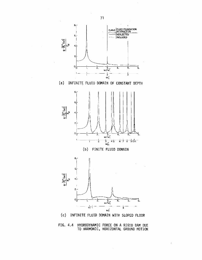
71

8.

CURVE FWID-FOUNDATIONINTERACTION

6.

4.

LJrl

2.

-- NEGLECTED---- INCLUDED

00 I. 2. 3. r 4. 5. 6.w/w,, ,

2 3w.i

n


8.

6.

4.A1\

LJ'\

2. I\\~, 1\

o \~) V (\-eJ-\. LJ~~ l) ,_o I. 2. 3' r 4. 5. 6.

w/w,L __---.L_----!c-'_-",~_+,+'_+'~'~I,_____,!'~Il,-

2 3 b 45 6 7 8 91011wm


8.

6.

4.

2.

.iwn

2

5. 6.

(c) INFINITE FLUID DOMAIN WITH SLOPED FLOOR

FIG. 4.4 HYDRODYNAMIC FORCE ON A RIGID DAM DUETO HARMONIC, HORIZONTAL GROUND MOTION

72

8.

6.

]~O I.l..t? 4.

2.

CURVE FLUID-FOUNDATIONINTERACTION



8.

6.

2.

I,.I'

"I', I

I'I,

II \ rlJ II I

\

-' I\,

! \I '_P

-~I ,'--

~ /

I. 2. 3' r 4. 6.W/W,

\, r ( ! , ! ! II

2 3 b 45 6 7 8 91011W m


:I I~I ,I I

]I.l..t? + \»

11.l..°-Cl

'LJ ~


FIG. 4.5 HYDRODYNAMIC FORCE ON A RIGID DAM DUETO HARMONIC, VERTICAL GROUND MOTION

73

and 3.32 (wi th q=0) reveals that in the nei ghborhood of -xFo(w)

due to horizontal ground motion is controlled by the term

lu/ - (w,{.)2f1/2, and FY (w) due to vertical ground motion by\' n -1 0

(w2- (w~) 2) . The second term approaches i nfi nity as w approaches

w~ faster than the first term; in fact, the ratio F~(w)/F~(w) of

hydrodynamic forces due to the two directions of ground motion

approaches infinity. The hydrodynamic force due to horizontal ground

motion is real valued at excitation frequencies below w~ and complex

valued at higher frequencies, whereas the force due to vertical ground

motion is real valued at all excitation frequencies.

In the case of the finite fluid domain, the hydrodynamic force

due to horizontal or vertical ground motion (Figs. 4.4b and 4.5b) is

unbounded at excitation frequencies equal to its eigenfrequencies

w~ (Sec. 3.2), which are more numerous than the w~ of the infinite

fluid domain of constant depth. The resonant frequencies w~ become

more densely populated in the low frequency range as the fluid domain

length is increased, but they always exceed w~ because the triangu

larly shaped domain always has an average depth smaller than the

domain of constant depth H. Examination of Eq. 3.11 reveals that

for the finite fluid domain, the hydrodynamic force due to either

direction of ground motion is controlled in the vicinity of w~ by-1

(w2 _ (w~)2) , similar to the term above for the infinite fluid

domain of constant depth subjected to vertical ground motion. The

hydrodynamic force due to either direction of ground motion is a real

valued function of frequency.

74

The hydrodynamic force on a rigid dam with the infinite fluid

domain with sloped floor is presented in Figs. 4.4c and 4.5c.

According to the discussion in Sec. 3.4, the hydrodynamic force is

real valued at excitation frequencies below w~ and complex valued

at higher frequencies. The force due to horizontal ground motion is

bounded at excitation frequencies equal to w~ (the eigenfrequencies

of the infinite region of depth ~ H), but unbounded at a frequency

w~ (Fig. 4.4c) which is less than wf. The response in the v"icinity

of w~ is real valued and has the resonant characteristics of a

finite fluid domain, hence the similar notation. This eigenfrequency

of the complete fluid domain (Sec. 3.4) is due to the sloped portion

of the reservoir floor which increases the average fluid depth to a

value greater than ~ H. The resonant peaks at higher frequencies in

Fig. 4.4c are bounded because of fluid-radiation damping. The hydro-

dynamic force due to vertical ground motion displays response charac-

teristics similar to those above, but with additional unbounded

responses at excitaton frequencies equal to w~. These unbounded

responses are due to the acceleration of the entire infinite length

of the reservoir floor; i.e., the acceleration vector ~ on the

right side of Eq. 3.39 is non-zero for vertical ground motion.

Because the geometries of the finite fluid domain and the infinite

fluid domain with sloped floor (Figs. 4.lb and c) are similar to a

distance H from the dam, the hydrodynamic forces associated with

the two fluid domains display similar resonse characteristics for

excitation frequencies up to the frequencies w~, which are nearly

the same as well for the two fluid domains.

75

4.2.2 Partial vertical excitation of the reservoir floor

The hydrodynamic force on a rigid dam due to a vertical accel

eration over a length Le of the floor of the infinite fluid domain

of constant depth is presented in Fig. 4.6. The frequency response

functions shown are for Le = H, 2H, and 00. Fluid-foundation inter

action is not included in this analysis. The force at excitation

ifrequencies equal to the eigenfrequencies wn is unbounded even when

Le is finite, but the resonant peaks are narrower indicating a

reduced response. In the vicinity of w~, the hydrodynamic force is

(2 . 2)-1/2

controlled by the term W - (w~) when Le is finite, in

contrast to the controll ing term (ci -(w~)2r1

when the ground

motion is over the entire reservoir floor. Thus, near w~ the fre

quency variation of hydrodynamic force due to vertical ground motion

over a partial length of the reservoir floor is similar to that due

to horizontal ground motion discussed in Sec. 4.2.1.


As shown in Figs. 4.4 and 4.5, the radiation damping associated

with fluid-foundation interaction reduces the hydrodynamic force

amplitudes. The reductions are primarily in the vicinities of the

resonant frequencies, resulting in bounded responses at these fre-

quencies for the three fluid domains considered and for both direc-

tions of ground motion. Due to fluid-foundation interaction, the

hydrodynamic forces are complex valued for all excitation frequencies

above zero.

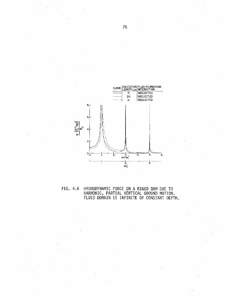
76

CURVE EXCITATION FLUID· FOUNDATIONLENGTH,Le INTERACTION

H NEGLECTED2H NEGLECTED<:J) NEGLECTED

8.

6.

"3~ -:;u.o IJ..'" 4.-0>

2.

I. 2.

:,

3. 4.W/W~

!

5.

3

6.

FIG. 4.6 HYDRODYNAMIC FORCE ON A RIGID DAM DUE TOHARMONIC, PARTIAL VERTICAL GROUND MOTION.FLUID DOMAIN IS INFINITE OF CONSTANT DEPTH.

77

4.3 Dam Responses to Horizontal Ground Motion

The responses of the dam to harmonic ground acceleration =

eiwt in the horizontal direction are presented for four conditions:

dam without water, dam with full reservoir considering water compres-

sibi1ity in one case but not the other (fluid-foundation interaction

neglected), and dam with full reservoir including both water com

pressibility and fluid-foundation interaction. These analyses were

perfonned for each of the three fluid domains of Fig. 4.1. Results

are presented in the fonn of complex frequency response functions

for accelerations of the dam relative to the ground acceleration

(Fig. 4.7). The absolute value (or modulus) of ~x(w), the horizon-

tal component of acceleration at the dam crest, is plotted against

the normalized excitation frequency parameter w/w1' where w1 = the

fundamental frequency of the dam. When presented in this form, the

results apply to similarly shaped dam-fluid systems of any height.

Furthermore, if the reservoir is empty or if the water is assumed

incompressible, the results are also independent of the concrete

elastic modulus Ed.


The response of the dam without water is representative of a

mu1ti-degree-of-freedom system with constant mass, stiffness, and

damping parameters. The presence of water, assumed to be incompres--f -fxsible, provides added masses 9j(0) and added load 90 (0).

Similar to the hydrodynamic force F~(O) on a rigid dam (Fig. 4.4a),

the added masses and added load are essentially unaffected by the

78

50. CURVE WATER FLUID'FOUNDATIONINTERACTION

40.

2. 3. 4. 5. 6. W/WI

I I I !I Wj2 3 4 56I I ! W~2 3 4

.......•- NONE----- INCOMPRESSIBLE NEGLECTED-- COMPRESSIBLE NEGLECTED

":: ---- COMPRESSIBLE INCLUDED

", ,

I.I

,""""" .11 ::

~J\<,, I, "o ..../

oI

10.

20.

30.


I

J I

2. 3. 4. 5. 6. W/W 1

I I I IIWj2 3 4 56

! ! Wi2 3 n


FIG. 4.7 HORIZONTAL COMPONENT OF DAM CREST ACCELERATIONDUE TO HARMONIC, HORIZONTAL GROUND MOTION

79

shape of the fluid domain. Consequently, if water compressibility

effects are neglected, the dam response is also essentially indepen

dent of fluid domain shape, and only responses of the dam with the

infinite fluid domain of constant depth are presented (Fig. 4.7a).

The resonant frequencies of the system are lowered and the resonant

amplitudes are increased.

When water compressibility is considered, the added masses

9!(w) and added load §~x(w) vary with excitation frequency in a

ma~ner similar to the frequency variation of F~(w) as discussed in

Sec. 4.2.1. At excitation frequencies where the 6f (w) vectors are

unbounded, the dam responses can only be computed from Eq. 2.23 as

limit solutions. For horizontal ground motion, these limits are

finite because the ratios of the terms of Qfx(w) to the terms of_0

§!(w) approach finite values. Thus, dam responses to horizontal

ground motion, with any of the fluid domains considered, are bounded

functions of excitation frequency.

For the infinite fluid domain of constant depth, inclusion of

water compressibility shifts the first resonant peak to a frequency

below wt, a greater shift with a greater increase in amplitude than

caused by incompressible water (Fig. 4.7a). These increases are due

to the greater hydrodynamic added mass and added load. At excitation

frequencies above wt, the §f(w) vectors are complex valued. The

imaginary part of the added mass vectors 6~(w) represents fluid-J

radiation damping which adds to the damping of the dam and reduces

the acceleration responses below those without water or with incom

pressible water.

80

When water compressibility is considered for the finite fluid

domain, the acceleration response of the dam displays many sharp

spikes throughout the entire frequency range (Fig. 4.7b). For finite

fluid domains, the hydrodynamic added mass and added load are real

valued functions of excitation frequency which are unbounded at fre

quencies equal to wb. Because the added mass in this case has nomimaginary component, the fluid domain adds none of the radiation

damping which occurs in an infinite fluid domain. The resulting dam

responses are affected greatly by the rapid variations with excitation

frequency of the hydrodynamic added mass and added load.

The acceleration response of the dam with the infinite fluid

domain with sloped floor is similar to its response with the finite

fluid domain in the lower part of the frequency range (Figs. 4.7b

and c), because the i/ (w) vectors vary with frequency in a similar

manner for the two fluid domains. This similarity was noted in-x ,(..

Sec. 4.2.1 with Fo(w). At excitation frequencies above wl ' fluid

radiation damping reduces the acceleration responses below those with

out water or with incompressible water, similar to the reductions

occurring with the infinite fluid domain of constant depth.


The effects of fluid-foundation interaction on the acceleration

response of the dam to horizontal ground motion are evident from the

two results of Fig. 4.7 which include water compressibility, and

include fluid-foundation interaction in one case but not the other.

Fluid-foundation interaction considerably reduces the dam accelerations

81

at excitation frequencies below wf if the fluid domain is infinite

(Figs. 4.7a and c) and throughout the entire frequency range when

the fluid domain is finite (Fig. 4.7b). These reductions are due to

the foundation radiation damping associated with the imaginary com

ponent of the added mass vectors Q~(w) and the smaller resonant-J

amplitudes of the added load vector §~x(w). Fluid-foundation inter-

action has significant influence on the dam accelerations only in the

frequency ranges where fluid radiation damping arising from an infi

nite extent of the reservoir does not exist.

Figure 4.7 also shows that the shape of the fluid domain has

little influence on the dam accelerations when fluid-foundation inter-

action effects are considered. For all three fluid domains, the

resonant responses of the dam including water compressibility and

fluid-foundation interaction are reduced in amplitude below those

without water and with incompressible water and have lower resonant

frequencies.

4.4 Dam Responses to Vertical Ground Motion

The responses of the dam to harmonic ground acceleration =

eiwt in the vertical direction over the entire reservoir floor are

presented in Fig. 4.8 for four conditions: dam without water, dam

with full reservoir considering water compressibility in one case but

not the other (fluid-foundation interaction neglected), and the dam

with full reservoir including both water compressibility and fluid

foundation interaction. These analyses were perfonned for each of

82

.-------- NONE----- INCOMPRESSIBLE NEGLECTED-- COMPRESSIBLE NEGLECTED---- COMPRESSIBLE INCLUDED

IFLUID-FOUNDATIONINTERACTIONCURVE WATER

4.[ [ [

2 3 4[ [ [ w..2 3 4 n

50.

40.

30.

"3>-:u.... 20.

10.

00


50.

4. 5116 Wj

I I I I II I I ! II I III I Wb6 8 10 12 1416 182021 m


50.

40.

30.

1>-:I.... 20.

10.

00 2. 3. 4. 6. W/w[

[ [ [ II Wj2 3 4 56[ [ I [ W ..

w~ I 2 3 n

(c)

FIG. 4.8

INFINITE FLUID DOMAIN WITH SLOPED FLOOR

HORIZONTAL COMPONENT OF DAM CREST ACCELERATIONDUE TO HARMONIC, VERTICAL GROUND MOTION

83

the three fluid domains of Fig. 4.1. Additionally, the response of

the dam with the infinite fluid domain of constant depth to vertical

ground motion, applied over a length Le = H or 2H of the reservoir

floor adjacent to the dam, is presented in Fig. 4.9. Fluid-foundation

interaction is neglected in this analysis. The dam responses are

presented as complex frequency response functions for accelerations

relative to the ground acceleration. The absolute value (or modulus)

of ~(w), the horizontal component of acceleration at the dam crest,

is plotted against the normalized excitation frequency parameter w/wl'

where wl = the fundamental frequency of the dam.


The resonant amplitudes in the acceleration response of the

dam without water to vertical ground motion are less than those due

to horizontal ground motion except for the third mode of vibration

(Fig. 4.3) which is dominant in vertical motion. If water is present

and assumed incompressible, the hydrodynamic effects in the dam

response to vertical ground motion are essentially independent of

fluid domain shape, and only responses of the dam with the infinite

fluid domain of constant depth are presented (Fig. 4.8a). The reso-

nant amplitudes are increased in some cases and decreased in others,

unlike the uniform increases that occur for horizontal ground motion

(Fig. 4.7a) indicating some cancellation between the dam's inertia

load and the hydrodynamic added load when the ground motion is

vertical.

84

l~hen water compressibility is considered and the fluid domain

is infinite, the dam response is unbounded at excitation frequencies

equal to w~(Figs. 4.8a and c). At these frequencies the added-f -f

mass and added load vectors Q.(w) and Qy(w) are unbounded-J -0

(similar to F~(w) and F~(w) of Secs. 4.2.1), and the limiting

values of the dam response from Eq. 2.23 are also unbounded. At

excitation frequencies below w~, the resonant response of the dam

to vertical ground motion exceeds that due to horizontal ground motion

because of the greater hydrodynamic added load. At excitation fre

quencies above w~ and between the infinite spikes in Figs. 4.8a

and c, fluid radiation damping limits the dam accelerations to about

those without water. Even though responses at excitation frequencies

equal to w~ approach infinity, they do so at a slow enough rate so

that the areas under the unbounded peaks are finite. Thus, the

Fourier Transform procedure of Sec. 2.4 for computing responses to

arbitrary ground motions is applicable.

When water compressibility is considered and the fluid domain

is finite, the acceleration responses to vertical ground motion dis-

play many sharp spikes throughout the entire frequency range

(Fig. 4.8b), as does the response to horizontal ground motion. This

similarity is due to the similar frequency variations of the hydrody

namic added loads for both directions of ground motion, as seen in

Sec. 4.2.1 for F~(w) and F~(w). In the lower portion of the fre

quency range, the accelerations of the dam with the finite fluid

domain are similar to those with the infinite fluid domain with

85

sloped floor (Figs. 4.8b and c), which was also true of the accelera-

tion respones to horizontal ground motion.

4.4.2 Partial vertical excitation of the reservoir floor

As noted in Sec. 4.4.1, the responses of dams with infinite

fluid domains to vertical ground motion are unbounded at excitation

frequencies equal to w~. Figure 4.9 shows that for the infinite

fluid domain of constant depth, these unbounded responses are reduced

to bounded values if the vertical acceleration is limited to a finite

length Le of the reservoir floor adjacent to the dam. At the fre

quencies wi, the added loads 6fy (w) resonate within narrower fre-n _0

quency bands when L is finite (similar to FY(w) of Sec. 4.2.2)e 0

causing the limit solutions of Eq. 2.23 to be bounded. From Fig. 4.9,

the acceleration responses decrease as L decreases, and largee

reductions occur in the vicinity of w~.


The responses of the dam at excitation frequencies equal to

iwn' which are unbounded if the fluid domain is infinite and subjected

to full vertical ground motion, are reduced to bounded values. This

is a consequence of the added load 9~Y(w) being a bounded function

of excitation frequency when fluid foundation interaction is included.

And as in the case of horizontal ground motion, fluid-foundation

interaction considerably reduces the acceleration responses of the dam

at excitation frequencies below w~ if the fluid domain is infinite

(Figs. 4.8a and c) and at all frequencies if the fluid domain is

finite (Fig. 4.8b). The dam accelerations including fluid-foundation

86

50. FLUID-FOUNDATIONCURVE WATER INTERACTION--------- NONE NEGLECTED

40. ----- INCOMPRESSIBLE NEGLECTED-- COMPRESSIBLE NEGLECTED

30.

3»:1"- 20.

"10., .--,

..

..,:~':'/\~-:.';..~_!'_--- ../ ---:-4"~':~~

00 ' I. 2. 3. 4. 5. 6.W/W,

I I I II2 3 4 56

WjI I I2 wL 3 4

n

(a) Le = H

50.

40.

30.

3»:1.... 20.

10.

00- - -- -

3. 4.W/w,

I I I II2 3 4 56

WjI I I2 w..· 3 4

n

(b) Le = 2H

FIG. 4.9 HORIZONTAL COMPONENT OF DAM CREST ACCELERATION DUE TOHARMONIC t PARTIAL VERTICAL GROUND MOTION. FLUID DOMAINIS INFINITE OF CONSTANT DEPTH. Le IS THE EXCITATION LENGTH.

87

interaction appear to depend somewhat more on fluid domain shape

than do the acceleration responses to horizontal ground motion.

When the ground motion is vertical, the hydrodynamic added load is

a more significant fraction of the dam's inertia load; consequently,

differences in the hydrodynamic added load due to fluid domain shape

have a greater effect on the acceleration responses to vertical

ground motion.

Acceleration responses of the dam to vertical ground motion

considering water compressibility and fluid-foundation interaction

(Fig. 4.8) generally exceed those responses without water and with~ bincompressible water especially in the vicinity of wl or wl

where the hydrodynamic added load is large. These increases contrast

to the reductions in the acceleration response of the dam to horizon-

tal ground motion when water compressibility and fluid-foundation

interaction are considered. The result is an increased importance

of the vertical component of ground motion on the dam accelerations

to a level comparable to the horizontal component.

89

5. HYDRODYNAMIC EFFECTS IN RESPONSE OF EARTH DAMS


The earth dam-fluid system investigated is shown in Fig. 5.1.

The dam is symmetrical about a vertical center line with equal

upstream and downstream slopes of ~:l . To emphasize hydrodynamic

effects, S is chosen as 1.5 resulting in a slope that is steeper

than those commonly used for earth dams, but typical of rock-fill

dams. The fluid domain is of infinite length and constant depth H

(equal to the dam height Hs ) beyond the toe of the dam. It is of

the infinite, irregular type discussed in Sec. 3.4.

The dam is modeled in a continuum state as a linearly elastic

shear beam. Such a representation is adequate for the present pur-

pose of investigating hydrodynamic effects on the dam response. A

shear wave velocity Cs within the dam of 2000 ft/sec, an upper

bound value, is chosen to emphasize hydrodynamic effects. Also, for

the dam, Ws = 130 pcf and ~j = 10% for each mode of vibration.

The fluid domain is discretized by the mesh of Fig. 5.2 which employs

two-dimensional elements with quadratic shape functions. For the

fluid domain, w = 62.4 pcf, C = 4720 ft/sec,and the reflection

coefficient a r = .85.

Results presented in this chapter are complex frequency response

functions due to harmonic ground acceleration = eiwt the horizontal

component of hydrodynamic force Ft(w) on a rigid dam and the accel-oeration ~t(w) of the dam crest relative to the ground acceleration.

-f -ftThe vectors Q.(w) and Q (w) of Eq. 2.24 are obtained as described-J -0


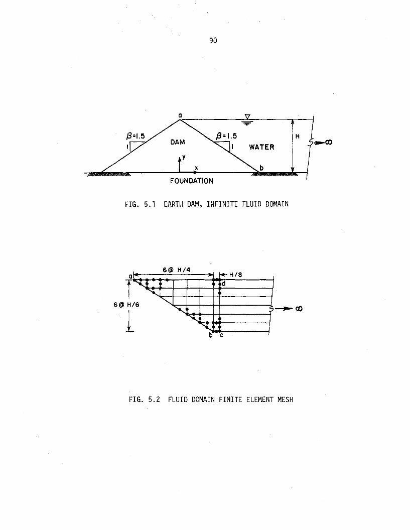
90

-;-

HDAM

WATERy

x b

FOUNDATION

FIG. 5.1 EARTH DAM, INFINITE FLUID DOMAIN

b c

I

""'li..j • d

"-16 """~ ?

~

~

6@ H/4al4l.~------"'.1 /+ HIS

T6@ H

1

FIG. 5.2 FLUID DOMAIN FINITE ELEMENT MESH

-f1(and pw)_0

twelve

91

in Sec. 3.5 from hydrodynamic pressure solutions p~(w)-J

-1 . flof Eq. 3.39. F (w) is also computed from p (w). Allo _0

eigenvectors ~n are employed in Eq. 3.39."1The dam accelerations r (w) are obtained from the modal

-responses Yj(w) computed from Eq. 2.23. For a triangular shear

beam model of the dam with the width varying linearly with height,

the terms of Eq. 2.24 related to the dam are available as continuum

expressions (15). The jth undamped mode shape is given by the

Bessel function of the first kind of order zero:

(5.l)

where the displacements defined by ¢j(y) are horizontal and result

from the shearing actions of the dam; and where T. = the jth zeroJ

of Jo' (T. = 2.40,5.52,8.65, ... ) The vector ¢! of Eq. 2.24J _J

contains only horizontal OOF and lists the values of ¢j(y) which

occur at the heights of the nodal points along a - b in Fig. 5.2.

The jth natural frequency of the dam is given by

(5.2)

Neither ¢j(y) nor wj depend on the slope S. The jth modal

mass is found as

92

wM. = 13 H2 -2.. i (Tl )

J s g 1 (5.3)

where Jl is the Bessel function of order one. C. and K. areJ J

determined from Eq. 2.6. The inertia loading terms for the jth dam

mode for ground motions in horizontal and vertical directions are

2 w Jl(Tl )E~ = 213 H -2.. ---J s g T 1

(5.4)

E~ = 0J

E~ is zero because the shear beam assumption permits only horizontalJ

dam motions relative to the base.

These modes ~j(Y) together with their natural frequen

appear in Fig. 5.3. The analysis of this chapter was carrieddes w.J

out with the computer program EADFS (14).

The first three dam modes are employed here in the computation..~

of r (w).

5.2 Hydrodynamic Forces on a Rigid Dam

The absolute value of F~(w), the horizontal component of

hydrodynamic force on a rigid dam, is presented in Figs. 5.4a and b

for ground motions in the horizontal and vertical directions,

respectively. Included are results for the fluid domain of Fig. 5.1

which has a sloped dam-fluid interface and for the infinite fluid

domain of constant depth (Fig. 4.la) which has a vertical interface.

93

'-- --I._......... ~b

a

"- .....3L. ~b

a

'- ---K. ~b

FIG. 5.3 MODE SHAPES AND NATURAL FREQUENCIES OF THE DAM

94

F~(w) is normalized with the horizontal component of hydrostatic

force Fst = tWH2 and w with w~ = rrC/2H. The plotted results

are independent of water depth H. Effects of water compressibility

and fluid-foundation interaction are described below.


The hydrodynamic force varies with excitation frequency if

water compressibility is considered. Whereas the hydrodynamic force

on the vertical face is unbounded at frequencies equal to w~ (the

eigenfrequencies of the infinite region of depth H), the force on

the sloped face is a bounded function of frequency when the ground

motion is horizontal (Fig. 5.4a). Thus, this fluid domain with out-

ward sloping dam face has no eigenfrequencies. The sloped interface

irregularity reduces the average water depth to a value less than H.

Thus, any eigenfrequencies and their associated infinite responses

for such a fluid domain have to occur above the frequency wt. Such

occurrence, however, is impossible because the eigenproblem associated

with Eq. 3.39 is complex valued over this frequency range. Fluid

radiation damping, then keeps the responses to horizontal ground

motion bounded above wt. Figure 5.4a indicates that the sloped dam

face is a less efficient generator of hydrodynamic pressure than is

the vertical face (see also Fig. 3.14).

The hydrodynamic force due to vertical ground motion (Fig. 5.4b)

is unbounded at excitation frequencies equal to w~ whether the damn

face slopes or not, a consequence of the acceleration of the infinite

reservoir floor; i.e., the acceleration vector ~ on the right side

of Eq. 3.39 is non-zero. The resonant peaks in Fig. 5.4b for the

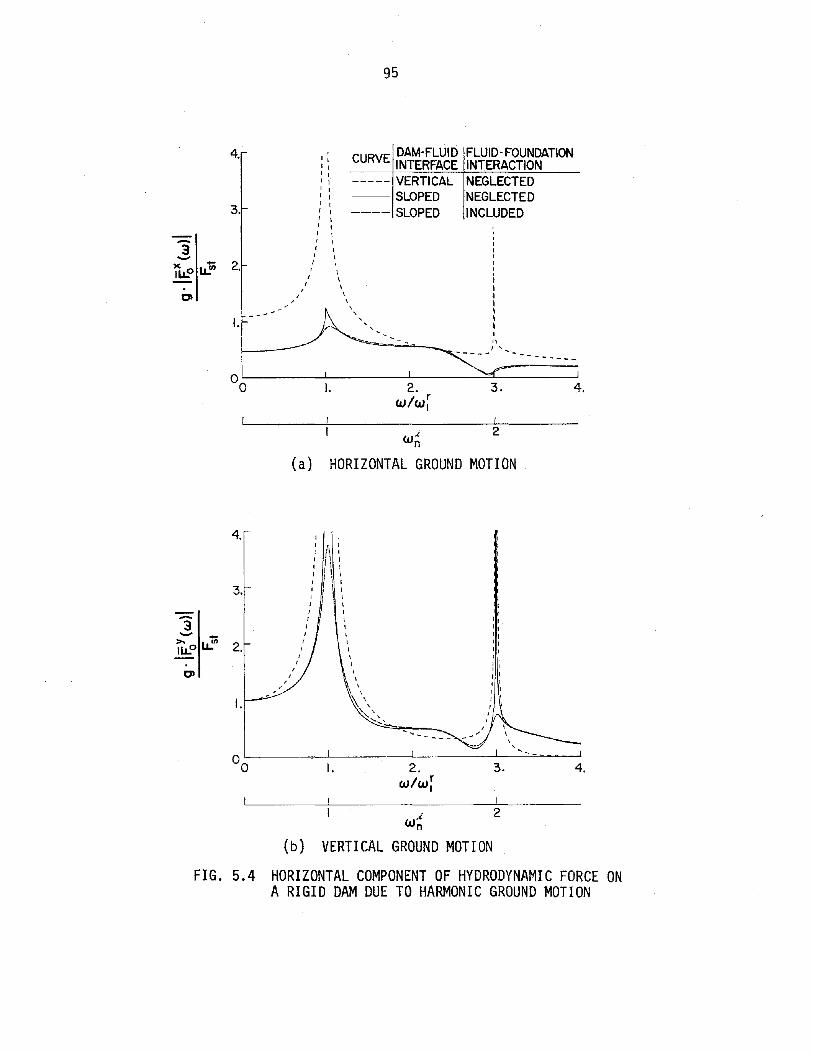
95

CURVE DAM-FLUID FLUID-FOUNDATIONINTERFACE INTERACTION

----- VERTICAL NEGLECTED-- SLOPED NEGLECTED---- SLOPED INCLUDED

4.

--- ------

,I,IIIII,IIIIIII

"II

3.2.w/wf

I.

,"I II II II II II II II ,

I II II ,I ,

I II ,

I \I \

I \" \/ \\ , , ,

4.

3.

-:3-ILL.° LL.1ii 2.

0-

I.

w.in

2


96

fluid domain with sloped dam face are narrower than those with the

vertical face, indicating a reduced response. With a rigid foundation,

responses of the fluid domain with sloped dam face are real valued

below wt and complex valued above for both directions of ground

motion.


When fluid-foundation interaction is considered, the hydrody

namic forces are bounded at all frequencies and complex valued for

w > O. The force amplitudes due to vertical ground motion (Fig. 5.4b)

are affected significantly by fluid-foundation interaction; the infi

nite responses at excitation frequencies equal to w~ are replacednby bounded peaks. The hydrodynamic force due to horizontal ground

motion (Fig. 5.4a) is affected only slightly.

5.3 Responses of the Dam

The absolute value of crest acceleration ~l(w) is presented

in Figs. 5.5a and b for horizontal and vertical ground motions,

respectively. The excitation frequency w is normalized with the

fundamental frequency of the dam wl' and the plotted results are

independent of dam height H. If the water is absent or incom-spressible, the results are also independent of shear wave velocity

Cs ' Because of the shear beam assumption, the dam response without

water is zero when the ground motion is vertical. Dam-fluid inter-

action effects and fluid-foundation interaction effects on the

acceleration response of the dam are described below.

97

I -------- NONE2 ----- INCOMPRESSIBLE NEGLECTED3 -- COMPRESSIBLE NEGLECTED4 ---- COMPRESSIBLE INCLUDED

FLUID·FOUNDATIONINTERACTION

3. 4. 5. 6.W/WI

I I2

W'3

J

CURVE WATER

2,3,4 !\, ,, ,: :, ,i \

1\: '"

,

10.

8.

6.-:3><:I~ 4.

2.

00

2


10.

8.

6.

:3->.:I~ 4.

2.

00

3,4- - - - - - - -I' - - - - - - -

I. 2. 3.w/w1

4. 5. 6.

2 3

w"n2


FIG. 5.5 ACCELERATION OF THE DAM CREST DUE TO HARMONIC GROUND MOTION

98


If the water is assumed to be incompressible, the hydrodynamic

effects are equivalent to frequency independent added masses Q:(O)-J

and added loads g~~(O). The resulting resonances in the acceleration

response to horizontal ground motion (Fig. 5.5a) occur at lower fre-

quencies with greater amplitudes than the resonances without water,

but the changes are smaller than those occurring in the response of

the concrete gravity dam (Fig. 4.7a). These hydrodynamic effects are

smaller for the earth dam because of its greater mass and its sloped

upstream face which, as discussed earlier, is a less efficient genera

tor of hydrodynamic pressures. For vertical ground motion (Fig. 5.5b),

non-zero response occurs although its amplitude is small.

If water compressibility is considered, then the hydrodynamic

force vectors Q:(w) and Qfx(w) vary with excitation frequency-J -0

similarly to the hydrodynamic force F~(w) on the rigid dam due to

horizontal ground motion (Fig. 5.4a), while 9~Y(w) varies similarly

to F~(w) due to vertical ground motion (Fig. 5.4b). Figure 5.4a

indicates that Q:(w) and Qfx(w) would be nearly independent of-J -0

frequency until just below wt. Thus, for this frequency range,

water compressibility has little influence on the acceleration

response to horizontal ground motion. Above wt water compressi

bility slightly decreases the dam accelerations because of fluid radi

ation damping associated with the imaginary component of the added

masses Q:(w). The response to vertical ground motion is unbounded at-J

excitation frequencies equal to w~ due to infinite values attained

by the added load Qfy(w). Thus, at these frequencies water compressi_0

bility has the effect of significantly increasing the dam accelerations.

99

Areas under the infinite spikes in Fig. 5.5 are finite, and the Fourier

Transform procedure of Sec. 2.5 for computing responses to arbitrary

ground motions is applicable.


Fluid-foundation interaction has a negligible effect on the

acceleration response to horizontal ground motion (Fig. 5.5a) because

of the similar Qf(w) vectors for rigid and flexible foundations (as

. seen in Fig. 5.4a with the similar F~(w) responses). Overall, hydro

dynamic effects are small in the response of the earth dam to horizon

tal ground motion. For vertical ground motion (Fig. 5.5b), fluid

foundation interaction replaces the unbounded responses at the w~

with small bounded peaks. No infinite responses can occur because the

added load Qfy(w) is now bounded. The acceleration response to ver-_0

tical ground motion including water compressibility and fluid-foundation

interaction is small compared to that to horizontal ground motion.

Thus, hydrodynamic effects are unimportant in responses of the earth

dam to both horizontal and vertical ground motions. And since the

chosen values for dam slope and shear wave velocity are extreme

values for earth dams to emphasize hydrodynamic effects, this conclu

sion is valid for earth dams in general.

101 Preceding page blank

6. THREE-DIMENSIONAL ANALYSIS PROCEDURE FOR DAM RESPONSE

6.1 Systems and Ground Motion

The three-dimensional structural behavior of an arch dam must

be considered in analyzing its response to earthquake ground motion.

The reservoir may extend only a short distance upstream (Fig. 6.1a)

or to a large enough distance so that it can be considered infinite

for purposes of qnalysis (Fig. 6.1b). In the latter case~ the reser-

voir cross-section is assumed to be uniform beyond some point in the

upstream direction. 'Behaviors within the elastic dam and compressible

water are assumed to be linear.

The earthquake ground motion is defined by the upstream

downstream (x)~ cross-stream (z)~ and vertical (y) components

of acceleration. With a rigid foundation (Sec. 6.2), no interaction

takes place between the dam and foundation or between the fluid and

foundation. Ground motions at all points along the foundation boun-

daries of the dam and fluid are the same. To approximately consider

fluid-foundation interaction effects (Sec. 6.3), the ground motion

along the reservoir floor and sides is described by free-field accel

erations which are assumed uniform. The actual acceleration of these

boundaries depends on the interaction.

and 2.24:

102

(a) FI NITE FLUID DOMAIN

WATER

(b) INFINITE FLUID DOMAIN

FIG. 6.1 THREE-DIMENSIONAL ARCH DAM-FLUID SYSTEMS

where

103

J/,= ~ (w), J/, = x,y,z (6.1)

(6.2)

and where y~w) = a vector of complex frequency response functions

for generalized displacements of the first J undamped natural modes

of vibration of the dam. The remaining terms of Eq. 6.1 are discussed

below in a three-dimensional context referring to the arch dam

infinite fluid domain system of Fig. 6.2.

The arch dam of Fig. 6.2 is discretized with finite elements.

The first J natural frequencies wj and mode shapes Pj are com

puted from the eigenproblem

2k<jJ.=w.m<jJ.- -J J - -J

(6.3)

where ~ and ~ = symmetric mass and stiffness matrices for the finite

element system. Only DOF for interior nodes not along the dam

foundation boundary are included in Eq. 6.3. <jJ~ in Eq. 6.2 lists the-J

x, y, and z components of the dam's jth mode shape for all nodes

along the dam-fluid interface a-b-c-d-a. M., C., and KJ. are the

J J

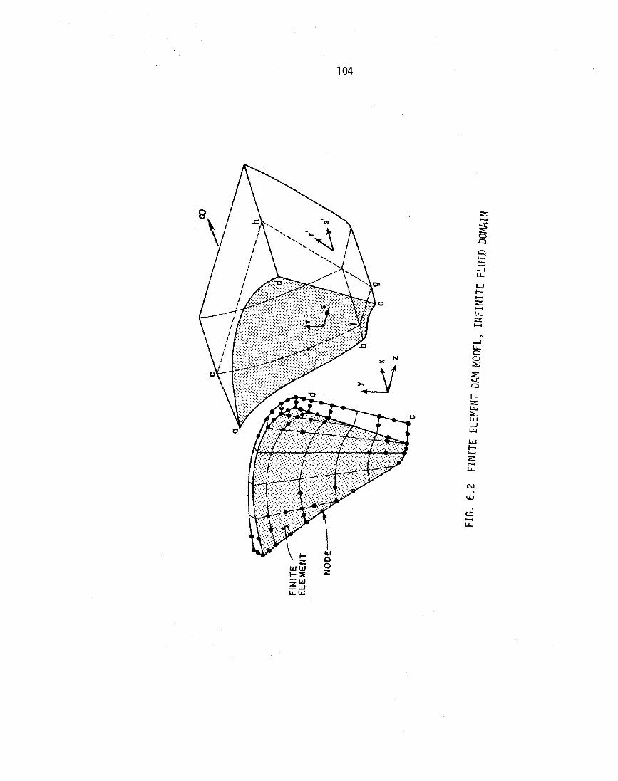
104

z......

~0.

0.......:::J...../u..LUIe......Z.......u..:z......

...../Wo~

~Ie:zw:E::w...../W

wIe-.......Z.......u..

N.l.D

105

jth modal mass, damping, and stiffness defined by the following

equations:

TMJ. = <t>. m <t>. ( 6•4a )

~J - -J

C. = 2 t,:. w. M. (6•4b )J J J J

2K. = w. M. (6. 4c )J J J

where i;j = the jth modal damping ratio. E£ is a vector of inertia

forces on the dam arising from a unit acceleration of the dam as a

rigid body in the £ direction. m is a mass matrix coupling OOF-gon the dam-foundation boundary with the interior OOF (non-zero for

consistent mass matrices only). The ith term of ~£ equals the

length of the component of a unit vector along £ in the direction

of the ith translational DOF. The vectors ~x, eY and ~z, for

ground motions in the x, y and z directions, contain ones in

positions corresponding to x, y and z translational OOF,

respectively, with zeros elsewhere.

-H( ) -f( )Q w, £= x,y,z and Q. w in Eq. 6.2 account for effects-0 -J

of the fluid and are associated with various boundary conditions pre-

sented below. All are vectors listing the x, y, and z components

of hydrodynamic forces on the dam at the dam-fluid interface with terms

ordered to correspond to those of ~;. The force vectors are computed

from hydrodynamic pressures on the dam-fluid interface by the method

of virtual work. Hydrodynamic pressures p(x,y,z,w) within the fluid

106

domain obey the three-dimensional Helmholtz equation:

(6.5)

Along accelerating fluid boundaries, the pressures should satisfy

s,r =s,r or s',r l (6.6)

where s,r = coordinates over the dam-fluid interface, and sl,r' =

coordinates over the reservoir floor and sides as shown in Fig. 6.2;

a (s,r) = normal component of boundary acceleration; and n denotesn

the inward normal direction to a boundary. Other boundary conditions

to Eq. 6.5 include the zero pressure condition at the free surface

(y = H)

p(x,H,z,w) = a (6.7)

and the radiation condition for infinite fluid domains.

g-oft(.w) . bt' d f th -ft() 1 th1S 0 a1ne rom e pressures Po s,r,w a ong e

dam-fluid interface arising from accelerations of the foundation in

the direction t while the dam is rigid. For this case, an(s,r)

from Eq. 6.6 is defined as

t= £ (s,r), s,r =s,r or s',r l (6.8)

107

where E~(s,r} = a function defined over accelerating boundaries which

gives the length of the component of a unit vector along ~ in the

direction of the inward normal n (a three-dimensional generalization

of the function E~(S) of Eq. 2.10). g!(w} is obtained from

p;(s,r,w} on the dam-fluid interface which arises from accelerations

of the dam in its jth vibration mode. Thus,

(6.9a)

(6.9b)

where ~;(s,r) = a continuous function representation of the component

of the jth mode normal to the dam-fluid interface.

6.3 Modifications to Include Fluid-Foundation Interaction

The acceleration boundary condition along the reservoir floor

and sides can be modified to approximately account for interaction

between the fluid and foundation in accordance with Sec. 2.5. The

portion of Eq. 6.6 along the reservoir floor and sides is replaced by

- ~ an(sl,r ' ) + iwq p(s',rl,w) (6.10)

where the damping coefficient q = w/wrC r ; wr and Cr = unit weight

and compression wave ve.10city of the foundation rock; and an(sl ,r ' )

is the free-field acceleration of the reservoir floor and sides defined

by Eq. 6.8 or 6.9b. The hydrodynamic force vectors g~~(w), ~=x,y,z

108

-f( ). -fJI,( ) -f(and Q. ware obtalned from the pressures p s,r,w and p. s,r,w)-J o· . J -

found as solutions to Eq. 6.5 subject to the boundary conditions of

Eq. 6.6 (dam-fluid interface), Eq. 6.10 (reservoir floor and sides),

and Eq. 6.7 with accelerations defined by Eqs. 6.8 and 6.9. Terms of

Eq. 6.2 related to the dam are unaffected.

The boundary condition Eq. 6.10 can be interpreted as the

result of idealizing the foundation as an assemblage of elastic,

independently acting columns of infinitesimal cross-section and

infinite length extending outward in a normal direction from the

reservoir floor and sides. This idealization and its implications

were discussed in Sec. 2.5.2.

109

7. THREE-DIMENSIONAL ANALYSIS OF HYDRODYNAMIC FORCE VECTORS

7.1 Boundary Value Problems and Solution Technigues

The hydrodynamic force vectors QfJ(,(w), Q,= x,y,z and Q~(w)-0 -J

of Eq. 6.2 are obtained from hydrodynamic pressure distributions

along the dam-fluid interface which are found by solving the three

dimensional Helmholtz equation:

(7.1)

subject to the acceleration boundary condition along the dam-fluid

interface

~an. (s,r,w) = - ~ a (s r)g n. '

(7.2a)

and along the reservoir floor and sides

~ (I I ) =an. s ,r ,w (7.2b)

the zero pressure condition at the free surface (y =H)

p(x,H,z,w) = 0 (7.3)

and the raditation condition for infinite fluid domains. Values of

the damping coefficient q in Eq. 7.2b greater than zero are used to

approximately account for fluid-foundation interaction effects; in

110

which case, a (s',r') is the free-field acceleration of the resern.

. voir floor and sides.

The accelerations in Eq. 7.2 are given by

s,r = s,r or sl,r' (7.4)

-f9-( )for computation of the hydrodynamic added load vectors go w,

9-= x,y,z . and by

(7.5a)

(7.5b)

for the hydrodynamic added mass vectors Q~(w). Corresponding solu-J

tions to the B.V.P.'s are p9-(x,y,z,w) and p.(x,y,z,w), respectively.o J

The gf(w) vectors are computed from pressures on the dam-fluid inter-

face by the method of virtual work.

Solutions to the above B.V.P.'s within finite fluid domains of

irregular geometry (Fig. 7.1) can be obtained by the finite element

method of Sec. 7.2. If the fluid domain is infinite but of uniform

cross-section, then the B.V.P. solutions can be obtained with the

finite element-continuum treatment of Sec. 7.3. Such a fluid domain

is shown in Fig. 7.2 and extends to infinity along the x axis with

uniform y- z cross-section. In this treatment accelerations of

the reservoir floor and sides can not vary in the x direction, but

can vary arbitrarily along the boundary of a y-z cross-section.

This requirement is consistent with the zero acceleration condition of

111

Eq. 7.5b and a1so~ since the fluid boundaries are straight in the x

direction~ with the E~(sl~rl) condition of Eq. 7.4.

The fluid domain of Fig. 7.3 has a finite region of irregular

geometry connected to a region that extends to infinity along the

x axis with uniform y- z cross-section. As described in Sec. 7.4~

solutions to the above B.V.P.1s can be obtained by a method utilizing

the standard finite element treatment of Sec. 7.2 for the finite

region and the finite element-continuum treatment of Sec. 7.3 for the

infinite region. Accelerations of the infinite region of uniform

cross-section can not vary in the x direction~ a requirement con-

sistent with Eqs. 7.~ and 7.5b.

The analysis procedures ofSecs. 7.2 to 7.4 are for hydrodynamic

pressures and are written for general accelerations rather than the

specific conditions of Eqs. 7.4 and 7.5. These conditions are con

sidered in Sec. 7.5 as is the actual computation of QH(w)~ ~= x,y,z-0

and Q~(w) from the resulting pressures along the dam-fluid interface.-J


Solution of the B.V.P. of Eqs. 7.1 to 7.3 within finite fluid

domains (Fig. 7.1a) can be obtained numerically by the finite element

method (12). The fluid domain is divided into three-dimensional e1e-

ments as shown in Fig. 7.1b. The resulting matrix equation

(Appendix B.3) takes the same form as Eq. 3.6:

(7.6)

112

c

(0) FLUID DOMAIM

h


FIG. 7.1 FINITE FLUID DOMAIN OF IRREGULAR GEOMETRY

113

where ~, ~, and § are symmetric matrices analogous to stiffness,

damping, and mass matrices arising in dynamics of solid continua;

E(w) = vector of unknown nodal pressures; and D= vector of nodal

accelerations computed from a (s,r) along the dam-fluid interfacen

a-b-c-d-a and a (s',r') along the reservoir floor and sidesnb-f-i-j-g-c-b, a-e-i-f-b-a, and d-h-j-g-c-d. The non-zero portion

of ~ is a submatrix corresponding to nodes along the reservoir

floor and sides where the boundary condition of Eq. 7.2b is applied.

Only DOF for nodes below the free surface are included in Eq. 7.6.

The pressures e(w) can be determined by solving the alge

braic equations (Eq. 7.6). For the case q = 0, e(w) can also be

determined using an eigenvector expansion with the real valued eigen-

vectors s resulting from the associated eigenproblem of Eq. 7.6:-m

(7.7)

The eigenvectors are orthogonal to ~ and G and are normalized

with respect to G. The result, following the procedure of Sec. 3.2,

takes the form of Eq. 3.11:

p_(w) =~ Z r- l ZT 0g - -

(7.8)

where the first M eigenvectors are included; and where ~ =

[~1'~2""'~M]; r = an MxM diagonal matrix with mth diagonal222term =Ym - w Ie; and Ym is the mth real valued eigenvalue from

Eq. 7.7. For q > 0, the above eigenvectors do not diagonalize ~

of Eq. 7.6.

114

pew) varies with excitation frequency as described in Sec. 3.2

for two-dimensional finite fluid domains. For q = a, the amplitude

of the mth eigenvector resonates to infinity at an eigenfrequency

w~ = ymC with opposite sign on each side. Thus, pew) is a real

valued function of frequency unbounded at the w~. For q > 0, p(w)

is bounded at all frequencies and complex valued for w > 0, which

are consequences of foundation radiation damping.

7.3 Infinite Fluid Domains of Uniform Cross-Section

7.3.1 Boundary value problems

The f1uid'domain of Fig. 7.2 extends to infinity along the x

axis with uniform y- z cross-section. The B.V.P. of Eqs. 7.1 to 7.3

is solved below for an acceleration a (y.z) of the dam-fluid interxface a-b-c-d-a and for an acceleration a (s',r ' ) = a~(r') of then n

reservoir floor and sides, unvarying in the upstream direction. The

coordinate s' is parallel to the x axis and r' follows the

boundary around a y - z cross-section. Sol utions are carried out

separately for these two acceleration conditions which are shown in

Figs. 7.2a and c.

The governing Eq. 7.1 with the boundary conditions

'* (O.y .z,w) = - '!!. a (y,z) (7. 9a)g x

~ ( , ) = iwq p(x. r' .w) (7.9b)Cln x.r.w

p(x.H,z,w) = a (7.gc)

.->..-l()1

.~""" ---J

(b) CHANNELDISCRETIZATIONOf fiG. a

a

(d) FINITEc

ELEMENT DISCRETIZATION

OF FIG. C

c

On(s"rl

) =o~{rl )

INFIN ITE CHANNEL

~NODALLINE

(el ACCELERATIONOF RESERVOIRfLOOR AND SIDES

c(a) ACCELERATION OF

DAM-FLUIDINTERFACE

FIG. 7.2 INFINI1E FLUID DOMAIN OF UNIFORM CROSS-SEC1ION

116

defines the first B.V.P. Equation 7.1 with boundary conditions

*(O,y,z,w) = 0

*(x,r',w) = - ~ a~(r') + iwq p(x,r',w)

p(x,H,z,w) = 0

defines the second B.V.P.

7.3.2 First B.V.P.

(7.10a)

(7.1 Ob)

(7.10c)

The uniform cross-section of this fluid domain allows the

x distribution of pressure to be separated from the y-z distribution.

Thus,

(7.11)


and Pyz(y,Z,w) must satisfy

2- 2-a Pyz a Pyz + 1 2 - = 0

2 + 2 A Pyzay az

(7.12a)

(7. 12b)

117

where K is a separation constant; and

(7.13)

Boundary conditions include Eq. 7.9a and the separated conditions

(7.l4a)

(7 .14b)

A finite element-continuum treatment is applied combining a finite

element eigensolution in the y- z plane with a continuum formulation

in the x direction. This process can be interpreted as a discretiza

tion of the fluid domain into channels of infinite length (Fig. 7.2b).

A finite element discretization of the eigenvalue problem defined by

Eqs. 7.12b and 7.14 using a two-dimensional mesh (Fig. 7.2d) takes the

form of Eq. 3.18:

(7.15)

whose derivation follows from that in Appendix B.l,and where the

matrices ~, ~~, and ~ are symmetric. The non-zero portion of

~~ is a submatrix corresponding to nodes along the boundary a-b-c-d

in Fig. 7.2d.

in Eq. 7.15.

Only DOF for nodes below the free surface are included

The ei genva1ues . An and ei genvectors Pn are complex

118

valued and dependent on the excitation frequency. The eigenvectors

are orthogonal and are normalized with respect to ~.

Following the procedure of Sec. 3.3.2, the vector of pressures

p(x,w) along the nodal lines below the free surface linesinFig. 7.2b

can be expressed in terms of the first N eigenvectors as

(7.16)

where! = [Pl'~2, ... ,PNJ; ~(x) = an NxN diagonal matrix with nth

-K xdiagonal term =en; and

K = VA2- ~ =]J + iVnn n C n

(7.17)

Kn is computed from Eq. 7.17 by taking the root with both ]In and

vn positive.

The vector of eigenvector amplitudes B(w) from Eq. 7.16 is

determined using the discrete form of the boundary condition Eq. 7.9a

(Appendix C.2):

. dp(f- d- (0,w) = - :!!. OX- x g - (7.18)

where ~ is the same matrix as in Eq. 7.15, and QX = a vector of

nodal accelerations corresponding to the acceleration ax(y,z) of the

dam-fluid interface. Solution for D(w) as in Sec. 3.3.2 and substi

tution back onto Eq. 7.16 results in

119

- ( ) w () K-1 \liT .DxE x,w = 9 Y~ X r (7.19)

which is of the same form as Eq. 3.27, and where ~ = an NxN diagonal

matrix with nth diagonal term = Kn. At x =0, Eq. 7.19 reduces to

(7.20)

Since Eqs. 3.27 and 7.19 are of the same form, the frequency

variation of e(x,w) from these equations will be similar. For

q = 0, An and Pn are real valued and frequency independent, and

Kn is real or imaginary depending on whether w is less than or

greater than AnC. Thus, p(x,w) is real for w < A1C, complex for

w > A1C, and unbounded at eigenfrequencies w~ = AnC. The part that

approaches infinity is real below each w~ and imaginary above. The

imaginary part of e(x,w) for frequencies greater than w~ is due

to fluid radiation damping. For q > 0, e(x,w) is bounded at all

frequencies and complex valued for w > 0, which are consequences of

foundation radiation damping.

7.3.3 Second B.V.P.

The B.V.P. of Eq. 7.1 with the boundary conditions of Eq. 7.10

is two-dimensional in the y,z coordinates. Omitting the x varia-

tions from these equations results in the two-dimensional Helmholtz

equation for p(y,z,w)

(7.21)

120

and the boundary conditions

.9i (r' w) =311 ~

p(H,z,w) = 0

(7.22a)

(7.22b)

Solution of Eq. 7.21 subject to the boundary conditions of

Eq. 7.22 can be obtained by the finite element method using a two

dimensional mesh (Fig. 7.2d). The finite element discretization of

this two-dimensional B.V.P. takes the same form as Eq. 3.31:

r~ + iwq si - w2

2 rfJ i1(w) :::: ~ If (7.23)L~ - c - c g -

whose derivation follows from that in Appendix B.1; and where ~,. .

~~, and ~ are the same symmetric matrices as in E~. 7.15; e(w) =

vector of unknown nodal pressures; and ~ = vector of nodal accelera

tions computed from a~(r!) along the boundary a-b-c-d. Only OOF11

for nodes below the free surface are included in Eq. 7.23.

If the N complex valued and frequency dependent eigenvalues

An and eigenvectors ~n of the associated eigenprob1em Eq. 7.15 are

available from a solution of the first B.V.P., then e(w) of Eq. 7.23

can be expressed in terms of these quantities as

(7.24)

121

which is of the same form as Eq. 3.32; and where A = an NxN diagonal

matrix with nth diagonal term = A~ - w2/c2. Note that A is

related to K from Eq. 7.19 by

A = K2 (7.25)

The frequency variation of e(w) is typical of finite fluid

domains. For q = 0, e(w) is a real valued function of w,

unbounded at the eigenfrequencies wi = A C with opposite sign onn n

each side. For q > 0, E(w) is bounded at all frequencies and com-

plex valued for w > O.


The fluid domain of Fig. 7.3a has a finite region of irregular

shape connected to a region extending to infinity in the x direc-

tion with uniform y- z cross-section. The plane of connection is

the y - z cross-section e-f-g-h-e. Normal accelerations of the dam-

fluid interface a-b-c-d-a and reservoir floor and sides are a (s,r)yt

and a (Sl r l ) respectively. Beyond e-f-g-h-e, ayt(sl,r l) = a~( r l

),yt , ,

unvarying in the x direction. In this region s I is parallel to

the x axis, and r l follows the boundary around a y- z cross-section.

Development of the finite element solution scheme follows the

procedure of Sec. 3.4. The finite region is discretized into three

dimensional finite elements (Fig. 7.3b) and-the infinite region into

channels (Fig. 7.3c) matching the adjacent mesh along e-f-g-h-e.

Equation 7.6 is written for the finite region with the unknown accel

erations normal to e-f-g-h-e represented by P~(w) (as in Eq. 3.34).

122

(a) IDEALIZED FLUIDDOMAIN

c

(b) FINITE ELEMENT DiSCRETIZATIONOF IRREGULAR REGION

FIG. 7.3 INFINITE FLUID DOMAIN OF IRREGULAR GEOMETRY

123

Application of the results of Sec. 7.3 to the infinite region leads

to a relation between Q~(w) and the pressures along e-f-g-h-e (as

in Eq. 3.38). Combining these two results leads to Eq. 7.26 which is

of the same form as Eq. 3.39:

T~. w2 1

! L~21 + lwq ~21 - C2 §21J

-!T~22 +;wq ~22 - ~~ §22] !+ ~

-

=

(7.26)

where only DOF for nodes below the free surface are included; and

where nodes along e-f-g-h-e are identified by subscript 2 and

remaining nodes by subscript 1. The finite element matrices

~11'~11' ... '§22 are written for the three-dimensional discretization

of the finite region. Ql and Q2 are acceleration vectors of groups

1 and 2 nodes computed from the accelerations of the exterior boun

daries of the finite region; i.e., the dam-fluid interface a-b-c-d-a

and the floor and sides b-f-g-c-b, a-e-f-b-a, and d-h-g-c-d. The

matrices ~, !' and D~ result from consideration of the infinite

region as described in Sec. 7.3.

Since Eqs. 3.39 and 7.26 are of the same form, the frequency

variation of el(w) from these equations will be similar. For q = 0,

el(w) is real valued for frequencies below the first eigenfrequency

124

iwl of the infinite region, and complex valued above due to fluid

radiation damping. Also, when. a~(rl) is non-zero, Pl(w) becomes

unbounded at each frequency w~ due to the infinite value attained

by the nth diagonal term of the matrix ~-l on the right side of

Eq. 7.26. Eigenfrequencies of the complete fluid domain and their

associated infinite responses can only occur below w~ where fluid

radiation damping is not present. For q > 0, el(w) is bounded at

all frequencies and complex valued for w > o.

7.5 computation of Hydrodynamic Force Vectors

For the fluid domains of Sees. 7.2 to 7.4, computation of the-n fhydrodynamic force vectors go (w), 5/,= x,y,z and Qj(w) of Eq. 6.2

proceeds as follows:

geometry) .Q,o and

-0

1. The boundary accelerations of Eqs. 7.4 and 7.5 are con

verted into acceleration vectors for use in Eqs. 7.6 or 7.8 (finite

fluid domain), Eqs. 7.20 and 7.24 (infinite fluid domain of uniform

cross-section), or Eq. 7.26 (infinite fluid domain of irregular

For the finite fluid domain, these vectors are denoted by

Qj' and their computation is described in Appendix 0.2.

Vectors {Ox}Q" Q,=x and {Ox}. of Eq. 7.20 and {0,}5/" {02}Q"-0 -J -0-0

Q,=x,y,z and {Ql}j' {Q2}j of Eq. 7.26 are computed similarly. Ini Q,

the latter case, {Q2}j = Q. {Q }o' Q,=y,z in Eqs. 7.24 and 7.26 is

computed with a~{rl) = £Q,{r ' ) similar to the procedure of Appendix 0.1,. Q, . .

and {Q-L}0' Q, =x and it} j of Eq. 7..26 are also zero vectors.

2. Using the acceleration vectors of step 1, hydrodynamic pres

sure vectors for a fluid domain are obtained by solving the appropriate

125

equations of Sec. 7.2, 7.3, or 7.4. Pressures along the dam-fluid

. -fR.() -f )interface are assembled lnto ~o w, R.= x,y,z and ~j(w.

3. As described in Appendix 0.2, the hydrodynamic force vec

tors are computed from the pressures along the dam-fluid interface

obtained in step 2.


8. HYDRODYNAMIC EFFECTS IN RESPONSE OF MORROW POINT DAM


Morrow Point Dam is a 465 ft, approximately symmetric, single

centered arch dam on the Gunnison River in Colorado. In the analy-

sis, it is assumed symmetric with dimensions averaged from the two

halves. The fluid domain is assumed symmetric also, to extend to

infinity in the upstream direction, and to have a water depth H

equal to the dam height. The dam-fluid system is shown in Fig. 8.1

where the plane of symmetry is the z = 0 plane, and the averaged

dimensions of the dam are listed in Table 8.1. The fluid domain

is of the infinite, irregular type described in Sec. 7.4; the reser-

voir cross-section is assumed to be uniform upstream of the y - z

plane e-f-g-h-e. System properties are chosen as Ed = 3 x 106 psi,

v = .2, wd = 150 pcf, w = 62.4 pcf, C = 4720 ft/sec, ar = .90,

and ~j = 5% for each mode of vibration of the dam. Ed' v and

wd are measured values of Morrow Point Dam (1).

Because the dam-fluid system is symmetric, dam and hydrody

namic pressure responses to upstream-downstream (x) and vertical

(y) ground motions are symmetric about the plane of symmetry, and

those due to cross-stream (z) ground motion are antisymmetric.

Only half the dam and fluid domain need be considered in the analysis

if appropriate boundary conditions along the plane of symmetry are

employed. In the analysis for x and y ground motions, the com

ponents of dam displacement and fluid acceleration normal to the plane

of symmetry are zero. The x and y components of dam displacement

128

I""a,e

y=279'

inw UNIFORMq-

--«> RESERVOIRy= 186'

IIIII

y=93'IIII CROSS-SECTIONII AT e=0° CANYONII y

CROSS - SECTIONSy=O'

IIf b, f z c

co

t , r--'--'---~---.----'

4@l50'

CANYONCONTOURS

SUPERIMPOSED PLANS AT93' ELEVATION INTERVALS

FIG. 8.1 MORROW POINT DAM, INFINITE FLUID DOMAIN

120'

20'

129

y T Td R Rd eu u

(ft. ) (ft. ) (ft. ) (ft. ) (ft. ) (0 )

465. 0.0 12. 375.0 363.0 56.20

372. 28.9 6.4 352.8 316.1 47.85

279. 46.3 0.8 324.9 258.0 39.50

186. 52.9 -2.6 296.5 210.8 33.00

93. 49.0 2.7 266.7 171.3 26.50

O. 34.4 17.2 234.8 136.6 13.25

TABLE 8.1 DIMENSIONS OF MORROW POINT DAM

130

and the hydrodynamic pressures at the plane of symmetry are zero for

the z ground motion analysis.

The finite element mesh for the dam appears in Fig. 8.2a.

The element employed is a shell element with quadratic shape functions

and eight nodes located at mid-thickness (16). The element has been

modified by removing an interior ninth node and by incorporating a

consistent mass matrix (1). Five degrees of freedom are associated

with each node: three translations and two rotations of the through-

thickness nodal line about axes perpendicular to its own axis. Normal

stresses perpendicular to the plane of the dam are assumed zero. The

finite element mesh for the fluid domain (Fig. 8.2b) employs three

dimensional elements with quadratic shape functions, and the plane

e-f-g-h-e is placed as close to the dam as possible to minimize the

number of OOF in the mesh. The dam and fluid domain meshes coincide

along the dam-fluid interface a-b-c-d-a.

Results presented in this chapter are complex frequency. iUltresponse functions due to harmonic ground acceleratlOn = e : the

x component of hydrodynamic force F£(w) on half a rigid dam ando

the radial acceleration ~i(w) of the dam crest relative to the-f -f£ground acceleration. The vectors Q.(w) and Q (w) of Eq. 6.2-J -0

are obtained as described in Sec. 7.5 from hydrodynamic pressure

1 · -f( ) -f£( ) - £( )so utlons p. wand p w of Eq. 7.26. F w is also computed-J _0 0

from pf£(w). The first 31 symmetric eigenvectors WS of the infi--0 _n

nite, uniform region are included in Eq. 7.26 for the x and y

ground motion analyses and the first 27 anti symmetric eigenvectors

~~ for the z ground motion analysis. These totals are the numbers

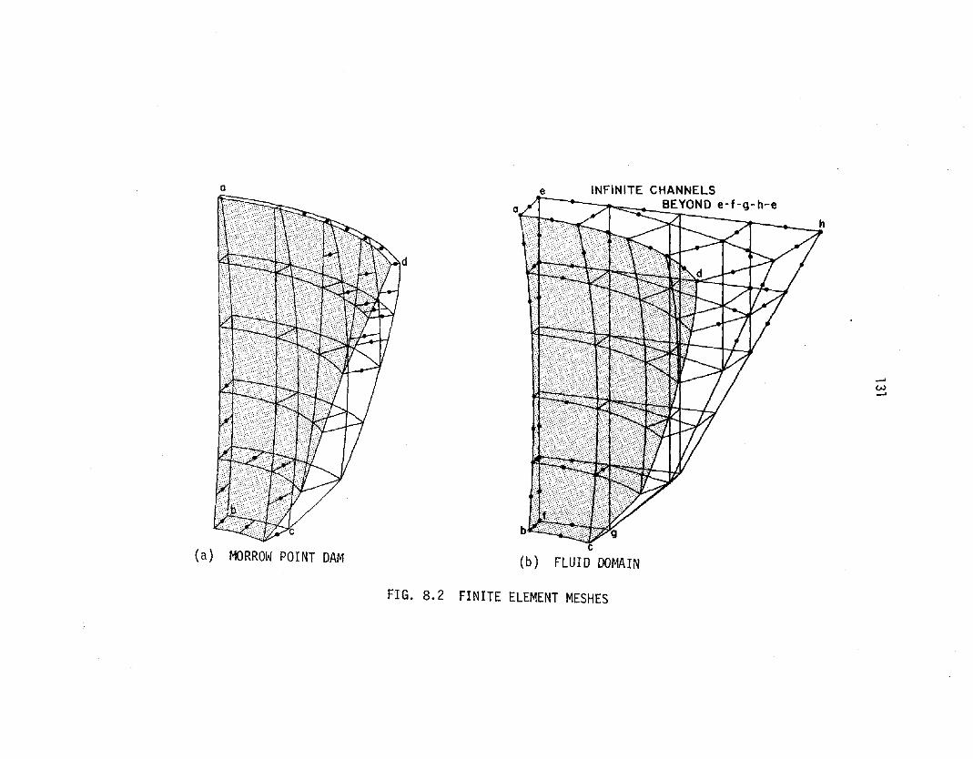
a

d

e INFINITE CHANNELSBEYOND e-f-g- h-e

-'w-'

(a) MORROW POINT DAMc

(b) FLUID DOMAIN

FIG. 8.2 FINITE ELEMENT MESHES

132

whose eigenfrequencies wisn

19.4 w~, where w~ = ~C/2H.

and wia (Sec. 7.3) are less thann

::~The dam responses r (w) are obtained

The first 12computed from Eq. 6.1.

are employed for x and y ground motion

12 anti symmetric modes ¢~ are employed for-J

the z ground motion analysis. Figures 8.3 and 8.4 show the first

from the modal responses

symmetric dam modes ¢~-J

analyses, and the first

8 symmetric and anti symmetric dam modes together with their naturals afrequencies wj and wj .

The analysis of this chapter was carried out with the computer

program EADFS (14). Solution times for computing the frequency

responses of the dam are presented in Appendix F.

8.2 Hydrodynamic Forces on a Rigid Dam-~The absolute value of FO(w) , the x component of hydrody-

namic force on half a rigid dam, is presented in Figs. 8.5a, band c

for ground motions in the x, y and z directions, respectively.-~Fo(w) is normalized with the hydrostatic force on the half dam

Fst = .208 wH2 and w with w~. When presented in this form, the

plotted results apply to similarly shaped fluid domains of any depth.

Effects of water compressibility and fluid-foundation interaction on-9-Fo(w) are described below.


When fluid-foundation interaction is neglected, the hydrodynamic ..'sforces are real valued at excitation frequencies below wl (x and

y ground motions) or below wta (z ground motion), and complex

133

PLAN ATy=465'

SECTIONAT 8=0 0

MODE \(31 =1.129

r-- -

,I

r-7I IL_J

MODE 2(32=1.624

.T--~

:::

\' ~-\".1 \

" 'f" \

\,~;\~. \\

1\\\

;[-, , ,, ,, ,,

!I

,,I

MODE :3/33 =1.8\0

MODE 4(34= 2.485

FIG. 8.3 SYMMETRIC MODE SHAPES OF MORROW POINT DAM.NATURAL FREQUENCIES ARE w~ = Sj J

d\!E9/Wd.

PLAN ATY=465'

SECTIONAT 8=0 0

134

:::z:.,, ', ', ,

, >-" ,, ,, ,, , ,, ,

MODE 5~5= 2.591

n1\

\\

\

I \

I II \I II \IIII

MODE 7,87=3.100

MODE 6~6 =2.805

C:=:=::t-_

n\

MODE 8~8= 3.648

FIG. 8.3 (CONTINUED)

PLAN ATY=465'

SECTION

AT 8= 13.25°

135

MODE 1f31=0.998

----:::c::::::-~-'"'~,>--

-- --- - -=-:t ..., ', ,

.............. >-" ,, ,, , ,, ,,

MODE 2f3 2= 2.031

-===::c::::-,--~ ......

----==:::::~., " ,.............. >...

" ,, , , ,, ,,

MODE 4f34 =3.039

FIG. 8.4 ANTISYMMETRIC MODE SHAPES OF MORROW POINT DAM.NATURAL FREQUENCIES ARE w~ = s. J- \!E9/Wd·

J J d

PLAN ATy = 465'

SECTiONAT e=13.25°

~--->-'-- --. ... :::z: -., ', ,

, ,'"" ,, , , ,, ,,

MODE 5/35= 3.237

MODE 7/37= 3.659

FIG. 8.4

136

(CONTINUED)

MODE 6/36 =3.469

MODE 8/38=4.109

137

valued at higher frequencies. The hydrodynamic forces due to x

ground motion (Fig. 8.5a) exhibit bounded peaks at frequencies equal

to w~s. Thus, no eigenfrequencies of the complete fluid domain

associated with symmetric responses exist. This beahvior, which is

dependent on the shape of the irregular portion of the fluid domain,

resembles that of the two-dimensional, infinite fluid domain with

sloped dam face described in Chapter 5.

Hydrodynamic forces due to y ground motion (Fig. 8.5b) are

unbounded at excitation frequencies equal to w~s, a consequence of

the accelerations of the floor and sides of the infinite, uniform

region; i.e., the acceleration vector ~ on the right side of

Eq. 7.26 is non-zero. Similarly, z ground motion (Fig. 8.5c) pro

duces unbounded hydrodynamic forces at frequencies equal to wia , asn

well as at a frequency w~a which is sl ightly less than wta . The

frequency w~a is an eigenfrequency of the complete fluid domain

associated with anti symmetric responses. This behavior, again

dependent on the shape of the irregular portion of the fluid domain,

resembles that of the two-dimensional, infinite fluid domain with

sloped floor described in Chapter 4. The resonances at wts due to

y ground motion and at w~a and wta due to z ground motion

involve large amounts of response and have greater amplitude over a

wider frequency interval than the x ground motion resonance at wts.

The resonance due to z ground moti on occurs at a much higher

frequency.

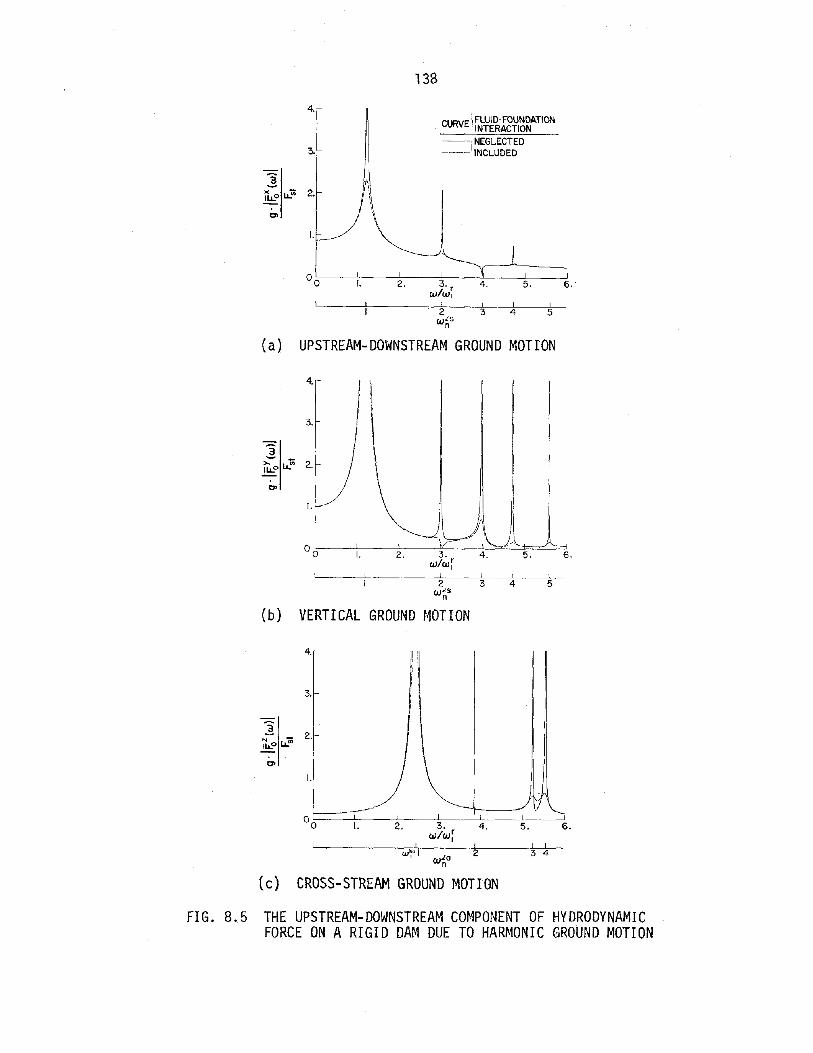
13B

4.

3.

CURVE FUJID-FOUNDATIONINTERACTION


I.

I. 2. 3. r 4. 5. 6.W/WI

I I I I

2 3 4 5w.iS

n

(a) UPSTREAM-DOWNSTREAM GROUND MOTION

4.

3.

"3~ -~o lL."' 2.-

0>

I.

°0 I. 2. 3. 5. 6.w/wi

~ I I I I

2 3 4 5w.iS

n


4.

3.

I.

I. 2. 3. 4.W/w;

II Iw~ol W.<o 2

n

I !

3 4

(c) CROSS-STREAM GROUND MOTION

FIG. 8.5 THE UPSTREAM-DOWNSTREAM COMPONENT OF HYDRODYNAMICFORCE ON A RIGID DAM DUE TO HARMONIC GROUND MOTION

139


The hydrodynamic forces due to each of the three directions of

ground motion are bounded functions of frequency and complex valued

for w > a when fluid-foundation interaction is included. Figure

8.5 shows that the amplitude reductions in the hydrodynamic force

F~(w) due to fl uid-foundation interaction are 1imited to vi cinities

of the resonant frequencies of the fluid domain. The resonances at

wts due to y ground motion and at w~a and wta due to z

ground motion are still significant and have greater amplitude over

a wider frequency interval than the x ground motion resonance atiswl .

8.3 Responses of the Dam:':.l/,

The absolute value of r (w), the radial component of dam

crest acceleration, is presented in Figs. 8.6, 8.7 and 8.8 for ground

motions in the x, y and z directions, respectively. Accelerations

at four locations along the dam crest are presented. As shown in

Fig. 8.8, the radial acceleration due to z ground motion is zero

at the plane of symmetry. The excitation frequency w is normalized

with the dam natural frequency w~ (x and y ground motion) or

w~ (z ground motion), and the plotted results apply to similarly

shaped dam-fluid systems of any height. If the water is absent or

incompressible, the results are also independent of the concrete

elastic modulus Ed. Dam-fluid interaction effects and fluid

foundation interaction effects are described below.

o I ~.(" 1--' D~

o I. 2. 3. 4.! I I I II 2 3 4 5

! I I! I! I I I I I1 2 3 4 5 6 7 8 9 10

I ~u ' _ - C1,_

--'....o

--c--~± W/w~

4.3.2.

CURVE I WATER 1FLUID-FOUNDATIONINTERACTION

--------- NONE----- INCOMPRESSIBLEI NEGLECTED-- COMPRESSIBLE NEGLECTED---- COMPRESSIBLE INCLUDED

o I -d ,.' I ----.--'--0f-' ~Ll--,--/ =:T W/w sD I. 2. 3. 4. I

I! I I I I WiSI 2 3 4 5 n

I I I I I I! ! ! I SI 2 3 4 5 6 7 8 9 \0 Wi

40.

50.

60.

70" 8= 13.250

30'1 Ih'I,

"

20'1 1\' I ,

, , ,r \ ,", I 1

I \ : ",

10.

0I.0

70'1 8=39.5 0

60.

50.

40.

30.

20.

10.

I'

, '.

j \L'\"

I,, \

I \

I \

" " 1\

,", ,, ,, ,, ,, ,, ,, \, ,,,,

\

I. 2. 3. 4.

10.,

00

20.,

70.[ 8=26.5 0

60.

50.~'

- 40.,3-)(:.... 30.

70r 8=00

60.

50.

'3 40.-)(

30.:1'-

20'1

10.

FIG. 8.6 RADIAL COMPONENTS OF DAM CREST ACCELERATION DUETO HARMONIC, UPSTREAM-DOWNSTREAM GROUND MOTION

.....~......

, ,

FLUID-FOUNDATIONINTERACTIONCURVE WATER

--._---- NONE----- INCOMPRESSIBLE NEGLECTED-- COMPRESSIBLE NEGLECTED---- COMPRESSIBLE INCLUDED

I~rlv \

\\'

~'I, ,

, \j"I, I1\ I \! \ I \

/ ,,- \

,/ ,'," ,--_.

o I .?' .-i~~....~ pL.- I ~ [ ..,,:=- -4"?t" W/W So I. 2. 3. 4. I'I 1 I I I W./S

I 2 3 4 5 nI I I I I I I I I I I w~

I 2 3 4 5 6 7 8 9 10 J

10.

50.

30.

40.

20.

70" 8=13.2~011 _60.

"j', ', ', '

,, ,, ,, ,,,

00 I. 2. 3.

70'1 8 =39.5°

60.

50.

40.

30.I' I I II I

20.I ,

I,, ,,

10." /1/ -- 11. - !, ,

o I -dY'- ....r ",=_ -< __ ).I..' "Y' ~-

o I. 2. 3. 4.1 1 [I! I

I 2 3 4 5I I! I 1/ I I t I I

I 2 3 4 5 6 7 8 9 10

70t8

=0°

60.r}IiI}\1'150.f- I

I

I\- 40t

\~ 30. ",, ,, ,, ,II I \

11

\ 'I20.f-1\ I \

1\ ! \, , ,, , ,

10'Ul

00

70r 8=26.5°

60.

50.

'3 40.->.:I~

10.

FIG. 8.7 RADIAL COMPONENTS OF DAM CREST ACCELERATIONDUE TO HARMONIC, VERTICAL GROUND MOTION

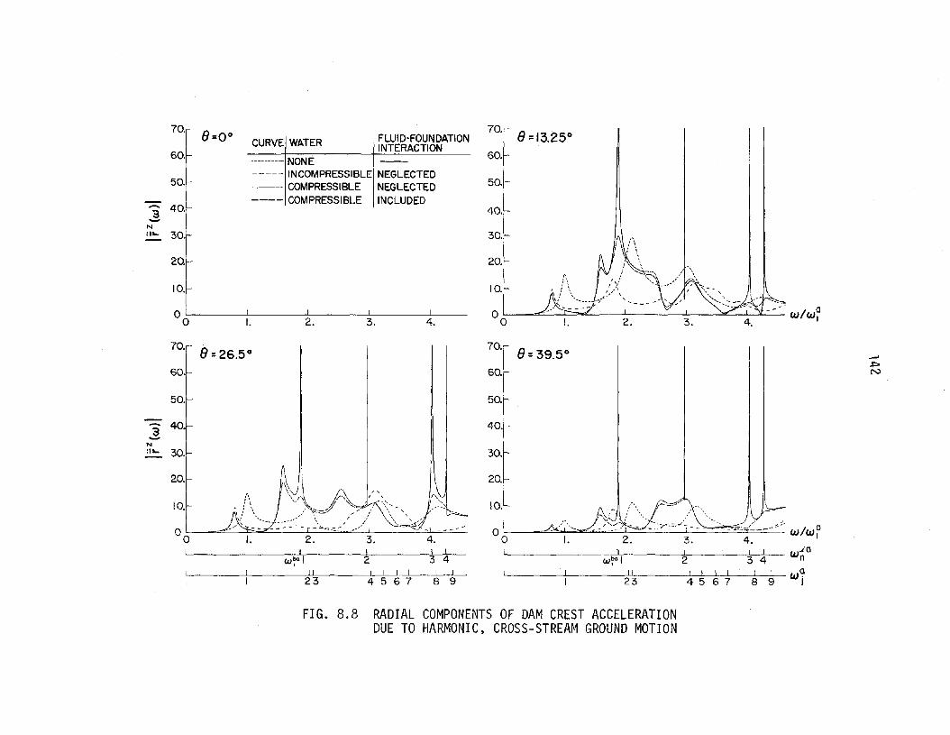
70.. 8=00CURVE WATER FLUID·FOUNDATION

70./ 8 =13.25°INTERACTION

60J- --------- NONE60.--

----- INCOMPRESSIBLE NEGLECTED50.1- -- COMPRESSIBLE NEGLECTED 50.

---- COMPRESSIBLE INCLUDED] 40.r- 40.

N:11- 30. 30.

20. 20.

10. 10.

0 1~., VI ~kf~

00

~'/' ',---,'" ~~....-../ ,---- I I ., --' W/Wo

I. 2. 0 l. 2. 3. 4. I

.......(::>0rv

8= 39.5°

o 1 ~-3-e! -~':l._:::> - ----- I - - ! - -- - --..=.--,. ---o I. 2. 3. 4.I U I I I W~·O

W~Q I 2 3 4 n\ \ \I I I \. \ 1 J W<:J

I 23 4 5 6 7 8 9 J

20.

10.

50.

60.

30.

40.

70.8 =26.5°

o \ ~~ ~- - \ - --=--:.- ~" I ......,- -1 - -

oU I I \

W~Q I 2 3 4I I II I I I I I I

I 23 4 5 6 7 8 9

10.

70.

60.

50.

- 40.~

N:,"- 30.

20.

FIG. 8.8 RADIAL COMPONENTS OF DAM CREST ACCELERATIONDUE TO HARMONIC. CROSS-STREAM GROUND MOTION

143


The dam accelerations without water due to x ground motion

exceed those due to y or z ground motion. If water is present

and assumed to be incompressible, the frequency independent added

mass and added load reduce the resonant frequencies and alter the

resonant amplitudes. These amplitudes are generally increased for

x and y ground motions (Figs. 8.6 and 8.7) but are decreased for

z ground motion (Fig. 8.8). The changes in resonant frequencies and

amplitudes are more pronounced for the arch dam than the concrete

gravity dam (Figs. 4.7 and 4.8) because the arch dam is lighter, and

hence, the hydrodynamic added mass and added load are relatively more

signficant fractions of the arch dam's mass and inertia load.

Water compressibility influences the dam responses through the

frequency variations of the af(w) vectors. The added load vectors

§~x(w}, §~y(w) and §~z(w) vary with excitation frequency simi

larly to F~(w), F~(w) and F~(w), respectively, of Fig. 8.5

(fluid-foundation interaction neglected). The added mass vectors

Q~(w) associated with symmetric dam modes vary similarly to FX(w};-J 0

the vectors Q~(w) associated with anti symmetric dam modes vary-J

similarly to FY(w), but with finite responses at the frequenciesoia Th .. . f -Qf() b is (d dwn . e lmaglnary part 0 _j w a ove wl x an y groun

motions) or above wta (z ground motion) provides fluid radiation

damping.

In the acceleration response to x and y ground motions

(Figs. 8.6 and 8.7), water compressibility further shifts the first

resonant peak to a frequency below wfs with a larger increase in

144

amplitude, a result of the greater hydrodynamic added mass and added

load. Dam accelerations due to y ground motion are unbounded at

excitation frequencies equal to w~s because of the infinite values

attained by 9~Y(w). The resonant amplitude of §~y(w) at wts

is large over a wide frequency interval (as for FY(w) in Fig. 8.5b)o

and results in very large dam accelerations in the vicinity

shown in Fig. 8.7. The increases in acceleration response

isof w1 asisnear w1

in Figs. 8.6 and 8.7 due to water compressibility exceed the corre

sponding increases in the concrete gravity dam response (Figs. 4.7 and

4.8). Thus, in this lower part of the frequency range, water com-

pressibi1ity appears to be more important for the arch dam than the

concrete gravity dam due to the greater relative importance of the

hydrodynamic forces. At excitation frequencies above wts , however,

this trend is offset due to a greater relative importance of fluid~sradiation damping for the arch dam. Above w1 ' the acceleration

response including water compressibility is smaller than the response

without water or with incompressible water in Fig. 8.6 and is reduced

to small values between the infinite spikes in Fig. 8.7.

The acceleration response of the dam to z ground motion

(Fig. 8.8) is unbounded at the frequencies w~a when water compressi-fz

bility is considered due to the infinite values attained by 90 (w).

The resonant amplitude of Qfz(w) near w~l'a is large over a wide_0

frequency range (as for F~(w) in Fig. 8.5c) and results in large damiaaccelerations in the vicinity of wl Whereas the large dam responses

~sto x and y ground motions near wl are due primarily to vibra-

tion of the dam in its first symmetric mode, the large response to

z ground motion near wfa (a significantly greater frequency than

145

wts ) is due to dam vibration in a combination of its second and third

antisymmetric modes. The response to z ground motion which is pri

marily of the first anti symmetric mode occurs at lower frequencies

Between the frequencies

in Fig. 8.8, fluid radiation damping limits the dam accelerationsiato small values. The infinite responses at the wn in Fig. 8.8 and

and is not affected by water compressibility.iawn

those at in Fig. 8.7 approach infinity at slow enough rates so

that the Fourier Transform procedure of Sec. 2.4 for computing

responses to arbitrary ground motions is applicable.


The Qf(w) vectors are bounded functions of frequency and com-

plex valued for w > 0 when fluid-foundation interaction is included.

Dam responses are affected by reduced resonances of the added load

vectors 6f~(w) and by the imaginary component of the added mass-0

vectors §!(w) which provides foundation radiation damping and which

is now present below w~s (x and y ground motion) or wta (z

ground motion).

Effects of fluid-foundation interaction on the acceleration

response to x ground motion (Fig. 8.6) are limited to a reduction

in amplitude of the first resonant peak located below wts Thus,

inclusion of water compressibility and fluid-foundation interaction

provides a general reduction in the dam accelerations below those

with incompressible water. However, the resonance below wt5 repre

sents an important increase in acceleration response in the low

frequency region compared to the response without water.

146

Fluid-foundation interaction effects on the acceleration

response to y ground motion (Fig. 8.7) include a bounded instead of

unbounded response at w~s, reduction of the preceding bounded peak.

and the elimination of the infinite spikes at the higher w~s.-fy isBecause go (w) still undergoes a large resonance at wl (as does

-y isFo(w) in Fig. 8.5b), the dam accelerations in the vicinity of wlare large and exceed greatly those accelerations without water or

with incompressible water. Above w~' however, the acceleration

response including water compressibility and fluid-foundation inter-

action is comparable in amplitude to the response without water and

is generally less than that with incompressible water.

In the acceleration response of the dam to z ground motion

(Fig. 8.8), the unbounded response at wfa is replaced by a bounded

peak, the preceding bounded peak is reduced, and the infinite spikes

at the higher w~a are eliminated because of fluid-foundation

interaction. The resulting dam accelerations are still greater than

those with incompressible water, and at some frequencies they are

greater than and at other frequencies less than those accelerations

without water.

Thus, the acceleration responses of the dam, including water

compressibility and fluid foundation interaction,to x and y ground

motions attain maximum amplitudes in the vicinity of wts and have

much lower response levels at higher frequencies. In the vicinity

of wts , the acceleration response to y ground motion has greater

amplitude over a wider frequency interval compared to the response to

x ground motion. For this reason, regarding dam accelerations, the

147

y component of ground moUon is likely to be of more importance than

the x component, a contrast to the dam accelerations without water

and with incompressible water where the x component of ground motion

is of greater importance. The relative importance of the z com

ponent of ground motion is uncertain and depends on the frequency

content of the ground time history because the region of maximum

response occurs in the vicinity of wta , a significantly greater fre

quency than wts . The large responses at wts due to x and y

ground motions are associated with hydrodynamic effects which appear

to be greater for the arch dam than the concrete gravity dam.

Preceding page blank149

9. CONCLUS IONS

Incorporation of finite element models of irregular fluid domains

into the substructure method for determining dynamic responses of dams

including hydrodynamic effects has proven successful. The finite ele

ment procedure applies to either two or three-dimensional fluid domains

and to either finite domains or infinite domains consisting of an irre

gular region of finite size connected to a region of uniform cross

section extending to infinity in the upstream direction. For such an

infinite uniform region, a finite element discretization within the

cross-section combined with a continuum representation in the infinite

direction provides for the proper transmission of pressure waves. The

fluid domain model can account for water compressibility and can approxi

mately account for fluid-foundation interaction with a damping boundary

condition applied along the reservoir floor and sides. The dam founda

tion is assumed rigid.

The substructure method is an effective way to compute dam

responses and include hydrodynamic effects. When water compressibility

is considered, the computational effort is greatly increased, and prac

tically all is spent to calculate the hydrodynamic terms which represent

effects of the fluid in the dam equation of motion. Thus, the computa

tional effort depends directly on the finite element mesh of the fluid

domain. The infinite, uniform reservoir assumption beyond some point

upstream of the dam will limit the finite element mesh to the region

between this point and the dam. Inclusion of fluid-foundation inter

action significantly increases the computational effort because most of

the arithmetic becomes complex valued. Further, for infinite fluid

150

domains the eigensolution associated with the infinite, uniform region

depends on the excitation frequency and for a three-dimensional fluid

domain will require a relatively large computational effort. Based on

the Morrow Point Dam example, the Central Processor times on a CDC 7600

computer for analyzing a three-dimensional dam-infinite fluid domain

system can be expected to be several hundred seconds if water compressi

bility is considered and from five to ten times this amount if fluid-

foundation interaction is considered (depending on symmetry considera-

tions and the extent of the finite element mesh).

Hydrodynamic effects due to water assumed to be incompressible

are equivalent to an added mass and added load which reduce the resonant

frequencies of the system and alter the resonant amplitudes. The added

mass and added load vary with excitation frequency if water compressi

bility is considered, and factors influencing the dam response include

resonances of the added load and the radiation damping associated with

the imaginary component of the added mass. If fluid-foundation inter-

action is neglected, this damping occurs only for infinite fluid domains

(fluid radiation damping) at frequencies above the first eigenfrequency

w~ of the infinite, uniform region (wts or wta for the three

dimensional symmetric or antisymmetric case), but occurs at all fre-

quencies for both infinite and finite domains if fluid-foundation inter

action is included (foundation radiation damping). Fluid-foundation

interaction also reduces the resonances of the added load which can be

very large if the fluid foundation is assumed rigid.

Hydrodynamic effects significantly influence the response of con-

crete gravity dams to harmonic ground motions, as seen with the complex

151

frequency response functions for the horizontal component of accelera

tion at the dam crest.

1. The dam accelerations with full reservoir are essen-

tially independent of reservoir shape if the water is

assumed to be incompressible. The resonant responses

of the dam generally exceed those of the dam without

water) but this does not hold for vertical ground

motion.

2. When water compressibility is considered, the dam

accelerations are very dependent on reservoir shape if

fluid-foundation interaction is neglected. For infi

nite fluid domains, the acceleration response of the

dam to horizontal ground motion at excitation fre

quencies above w~ is reduced by fluid radiation

damping below those responses without water and with

incompressible water. However, unbounded responses to

vertical ground motion cccur at excitation frequencies

equal to w~ if the vertical excitation is applied

over the entire length of the infinite reservoir floor.

Frequency ranges where fluid radiation damping is not

present, below w~ for infinite fluid domains and at

all excitation frequencies for finite fluid domains,

are regions of high response which can vary rapidly

wi th frequency.

152

3. Inclusion of fluid-foundation interaction reduces these

large responses and reduces the unbounded responses that

occur for infinite fluid domains under complete vertical

ground motion to bounded values. The resulting dam

accelerations depend much less on fluid domain shape,

especially for horizontal ground motion. Compared to

the accelerations without water and with incompressible

water, the acceleration response to horizontal ground

motion including water compressibility and fluid-

foundation interaction is reduced, and that to vertical

ground motion is increased especially in the vicinity

of the first resonant frequency of each fluid domain.

The result, regarding dam accelerations, is a comparable

level of importance for both horizontal and vertical

components of ground motion.

Hydrodynamic effects in the acceleration response of earth dams

to harmonic ground motions were investigated by employing a shear beam

model for the dam. In the response to horizontal ground motion, hydro-

dynamic effects are unimportant due to the large mass of the dam and the

small hydrodynamic pressures produced by the accelerations of the sloped

dam face. If the ground motion is vertical, the dam response without

water is zero because of the shear beam assumption, and that with incom-

pressible water is small. For the infinite fluid domain considered, the

dam response to vertical ground motion considering water compressibility

is unbounded at excitation frequencies equal to w~ if fluid-foundationn

interaction is neglected. However, inclusion of fluid-foundation

153

interaction reduces these unbounded responses to bounded values, and

the dam accelerations are again small compared to those due to horizon-

tal ground motion. Thus, hydrodynamic effects are unimportant in the

acceleration response of earth dams to both horizontal and vertical

ground motions.

For Morrow Point Dam, an arch dam, hydrodynamic effects appear to

be more important than for the concrete gravity dam because the added

mass and added load are more significant fractions of the arch dam's

smaller mass and inertia load. These effects were investigated for the

frequency response functions of radial acceleration at the dam crest due

to harmonic ground motion.

1. When the water is assumed incompressible, the resonant

amplitudes of acceleration responses to upstream-

downstream (x) and vertical (y) ground motions

generally exceed those of the dam without water, while

the resonant amplitudes due to cross-stream (z) ground

motion are decreased.

2. For the infinite fluid domain considered, water compres-

sibility produces large dam accelerations in the vicini-

. f'<'s (d d t' ) and ":<-1'atles 0 wl x an y groun mo lons w

(z ground motion), especially for y and z ground

motions where unbounded responses occur at these

frequencies. Dam accelerations above wts or wta

are much lower due to fluid radiation damping except for

infinite spikes which occur at the higher

(y ground motion) or

154

(z ground motion) due to

the non-zero accelerations of the floor and sides of

the infinite reservoir.

3. Inclusion of fluid-foundation interaction eliminates

these infinite spikes, but large acceleration responses

still occur in the vicinities of wts (x and y ground

motions)or w~a (z ground motion). These dam accelera-istions near wl due to y ground motion greatly exceed

those due to x ground motion; thus, the y component

of ground motion is likely to be of more importance, a

contrast to the cases without water and with incompressi-

ble water where the x component is of more importance.

The relative importance of the z component of ground

motion depends on the frequency content of the earthquakeiatime history since the maximum responses occur near wl '

a significantly greater frequency than wts

The method of analysis needs to be improved to account for founda-

tion interaction with the dam. Such a provision should include realistic

free-field motions along the canyon walls in arch dam analyses. Regarding

computational efficiency, large savings would result from a more efficient

treatment of the frequency dependent eigenproblem associated with the

infinite, uniform region of a three-dimensional fluid domain when fluid

foundation interaction is considered. Several such schemes are currently

under study. Further work is needed to extend the investigation of

hydrodynamic effects on dam responses to earthquake ground motions,

including stress responses.

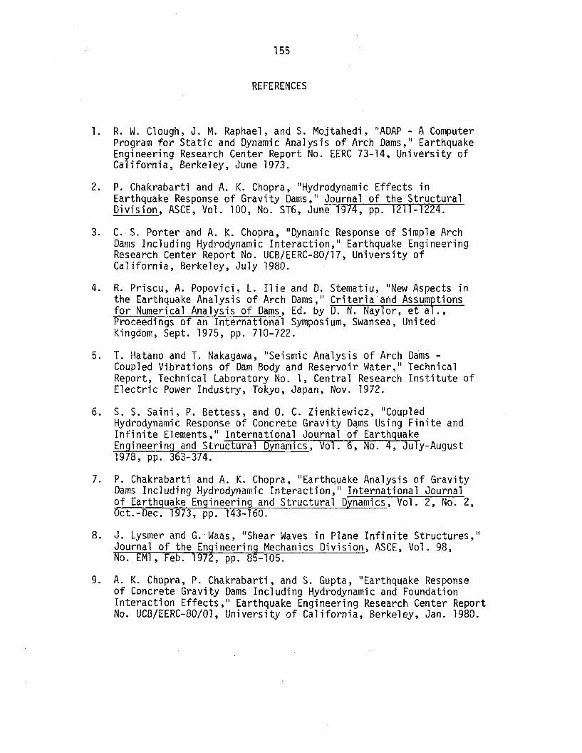
155

REFERENCES

1. R. W. Clough, J. M. Raphael, and S. Mojtahedi, "ADAP - A ComputerProgram for Static and Dynamic Analysis of Arch Dams," EarthquakeEngineering Research Center Report No. EERC 73-14, University ofCalifornia, Berkeley, June 1973.

2. P. Chakrabarti and A. K. Chopra, IIHydrodynamic Effects inEarthquake Response of Gravity Dams,1l Journal of the StructuralDivision, ASCE, Vol. 100, No. ST6, June 1974, pp. 1211-1224.

3. C. S. Porter and A. K. Chopra, "Dynamic Response of Simple ArchDams Including Hydrodynamic Interaction," Earthquake EngineeringResearch Center Report No. UCB/EERC-80/17, University ofCalifornia, Berkeley, July 1980.

4. R. Priscu, A. Popovici, L. !lie and D. Stematiu, IINew Aspects inthe Earthquake Analysis of Arch Dams," Criteria and Assumptionsfor Numerical Analysis of Dams, Ed. by D. N. Naylor, et al.,Proceedings of an International Symposium, Swansea, UnitedKingdom, Sept. 1975, pp. 710-722.

5. 1. Hatano and T. Nakagawa, "Seismic Analysis of Arch Dams Coupled Vibrations of Dam Body and Reservoir Water,1I TechnicalReport, Technical Laboratory No.1, Central Research Institute ofElectric Power Industry, Tokyo, Japan, Nov. 1972.

6. S. S. Saini, P. Bettess, and O. C. Zienkiewicz, IICoup1edHydrodynamic Response of Concrete Gravity Dams Using Finite andInfinite Elements," International Journal of EarthquakeEngineering and Structural Dynamics, Vol. 6, No.4, July-August1978, pp. 363-374.

7. P. Chakrabarti and A. K. Chopra, "Earthquake Analysis of GravityDams Including Hydrodynamic Interaction," International Journalof Earthguake Engineering and Structural Dynamics, Vol. 2, No.2,Oct.-Dec. 1973, pp. 143-160.

8. J. Lysmer and G.'Waas, "Shear Waves in Plane Infinite Structures,"Journal of the Engineering Mechanics Division, ASCE, Vol. 98,No. EM1, Feb. 1972, pp. 85-105.

9. A. K. Chopra, P. Chakrabarti, and S. Gupta, IIEarthquake Responseof Concrete Gravity Dams Including Hydrodynamic and FoundationInteraction Effects," Earthquake Engineering Research Center ReportNo. UCB/EERC-80/01, University of California, Berkeley, Jan. 1980.

156

10. E. Rosenblueth, "Presion hidrodinamica en presas debida a laaceleraci6n vertical c,.on r~fracci6n en el fondo, II II CongresoNacional de Ingenieria Sismica, Veracruz, Mexico, May 1968.

11. D. Rea, C-Y. Liaw, and A. K. Chopra, IIMathematical Models forthe Dynamic Analysis of Concrete Gravity Dams," InternationalJourna1 of Earthquake Engi neeri ng and Structural Dynami cs, Vol. 3,No.3, Jan.-March 1975, pp. 249-258.

12. O. C. Zienkiewicz, The Finite Element Method, McGraw-Hill BookCompany (UK) Limited, 1977.

13. A. 1. Chwang, IIPressures on Sloping Dams During Earthquakes.Part 2. Exact Theory,1I Journal of Fluid Mechanics, Vol. 87,Part 2, July 1978, pp. 343-348.

14. J. F. Hall and A. K. Chopra, "A Computer Program for EarthquakeAnalysis of Dam-Fluid Systems," Earthquake Engineering ResearchCenter Report, University of California, Berkeley (to bepub1 ished).

15. G. R. Martin and H. B. Seed, "Dynamic Response Analyses for EarthDams,1I Report No. TE 65-1, Institute of Transportation andTraffic Engineering, University of California, Berkeley,Aug. 1965.

16. S. F. Pawsey, liThe Analysis of Moderately Thick to Thin Shells bythe Finite Element Method," Report No. UC SESM 70-12, StructuralEngineering Laboratory, University of California, Berkeley,Aug. 1970.

17. K. J. Bathe, IISo1ution Methods for Large Generalized EigenvalueProb1ems in Structural Engi neeri ng, II Report No. UC SESM 71-20,Structural Engineering Laboratory, University of California,Berkeley, Nov. 1971.

18. D. P. Mondkar and G. H. Powell, IITowards Optimal In-CoreEquation Solving,1I Computers and Structures, Vol. 4, No.3,May 1974, pp. 531-548.

19. R. W. Clough and J. Penzien, Dynamics of Structures, McGraw-Hill,Inc., 1975.

157

APPENDIX A. NOTATION

J/,ag = component of ground acceleration in the JI, direction

a =component of acceleration normal to a fluid boundaryn .

a~ = component of acceleration normal to the boundary of theuniform cross-section of an infinite fluid domain

A,A,B,B = incident and reflected wave amplitudes employed in Sec. 2.5

A~ = Fourier transform of a~

B = finite element IIdamping li matrix for a finite fluid domain

B-!.. = finite element "dampi'ng" matrix for the uniform cross-sectionof an infinite fluid domain

c = finite element damping matrix for the dam

C = velocity of compression waves in water

Cj = generalized damping of the jth natural mode of vibrationof the dam

C = velocity of compression waves in the foundation rockr

C = velocity of shear waves in an earth dams

D = vector of nodal accelerations for a fluid domain

DX = vector of nodal accelerations at the dam-fluid interface ofan infinite fluid domain of uniform cross-section

D~ = vector of nodal accelerations for the uniform cross-sectionof an infinite fluid domain

DJ/, = vector of nodal accelerations due to a harmonic ground-0

acceleration = eiwt in the 1 direction with rigid dam

158

Qj = vector of nodal accelerations due to a harmonic accelerationof the dam in its jth natural mode of vibration

-K X~(x) = an Nx N di agona1 matri x wi th nth di agona1 term = e n

~~ = a vector defined for Eqs. 2.2 and 6.2

Ed =modulus of elasticity of concrete

Er =modulus of elasticity of foundation rock

E~ = vector of inertia loads on the dam due to a unit accelerationof the dam as a rigid body in the ~ direction

Fst = x component of force on the dam (or half of a symmetric dam)due to hydrostatic pressure

Ft = x component of hydrodynamic force on a rigid dam (or half ofoa symmetric, rigid dam) due to ground acceleration in the ~

direction

-t ~Fo = complex frequency response of Fo

9 = acceleration of gravity

G= finite element IImass " matrix for a finite fluid domain-G,(. = finite element "mass ll matrix for the uniform cross-section

of an infinite fluid domain

H= water depth adjacent to the dam

Hd = height of a concrete dam

H = height of an earth dams

H=finite element "stiffness" matrix for a finite fluid domain

H,(. = finite element "stiffness ll matrix for the uniform crosssection of an infinite fluid domain

159

i = A

J = number of ¢. included for the dam-J

JO,Jl = Bessel functions of the first kind of orders zero and one;respectively

k = finite element stiffness matrix for the dam

K. = generalized stiffness for the jth natural mode of vibrationJ

of the dam

~ = direction of ground motion, either x, y, or z

L = excitation length for the floor of an infinite fluid domaineof constant depth

L~ =generalized load for the jth natural mode of vibration ofJ

the dam including hydrodynamic added load and due to groundacceleration in the ~ direction

L~ = vector of dimension J with jth term = L~J

m = finite element mass matrix for the dam

m = mass matrix for the dam coupling DOF along the foundation-gwith interior DOF

M= number of s included for a finite fluid domain-m

M. = generalized mass for the jth natural mode of vibration ofJ

the dam

yt denotes the inward normal direction to a fluid boundary

N = number of 1/J included for an infinite fluid domain-n

p = hydrodynamic pressures in excess of static pressure

pf = pressures at the dam-fluid interface

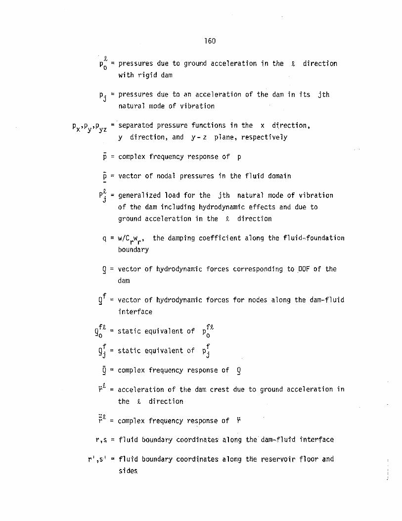
160

J/,Po ~ pressures due to ground acceleration in the t direction

with rigid dam

p. = pressures due to an acceleration of the dam in its jthJ

natural mode of vibration

Px,Py,PyZ = separated pressure functions in the x direction,y direction, and y- z plane, respectively

-p = complex frequency response of p

-p = vector of nodal pressures in the fluid domain

p~ = generalized load for the jth natural mode of vibrationof the dam including hydrodynamic effects and due toground acceleration in the J/, direction

q = w/Crwr , the damping coefficient along the flui.d".,foundationboundary

9 = vector of hydrodynamic forces corresponding to DOF of thedam

gf = vector of hydrodynamic forces for nodes along the dam-fluidinterface

QH = static equivalent offJI,

-0 Po

Q~ = static equivalent of fp.-J J

9= complex frequency response of 9

~J/, = acceleration of the dam crest due to ground acceleration inthe J/, direction

:':R,r = complex frequency response of r

r,s ;:; fluid boundary coordinates along the dam""fluid interface

r',s' = flutd boundarY' coordinates along the reservoir floor andsides

161

Ru,Rd = radii to upstream and downstream faces of an arch dam

s = the J x J dynamic stiffness matrix for the dam includinghydrodynamic added mass

t = time variable

t d = duration of ground motion

Tu,Td = thickness parameters to upstream and downstream faces of anarch dam

u = vertical foundation displacement

-u = complex frequency response of u

v = vector of nodal displacements of the dam relative to the ground

w = unit weight of water

wd = unit weight of concrete in a dam

wr unit weight of foundation rock

Ws = unit weight of earth in a dam

x,y,z = orthogonal coordinates in upstream-downstream, vertical, andcross-stream directions, respectively

v1 = generalized displacement of the jth natural mode of vibrationof the dam due to ground acceleration in the ~direction

~complex frequency response of V.J

vector of dimension J with jth

a = the reflection coefficient for an incident·pressure waverstriking the foundation rock

am = amplitude of s-m

-am = complex frequency response of am

162

a = vector of dimension M with mth term = am

8 = parameter defining the slope of an earth dam

Bj = parameter used to define the jth natural frequency of the dam

Ym=mth eigenvalue of a finite fluid domain (q =0)

_ 2 (}r = an MxM diagonal matrix with mth diagonal term - Y - 2"

m C

£~ = function defined for Eqs. 2.10 and 6.8

~m = mth eigenvector of a finite fluid domain (q = 0)

Z = matrix with the M eigenvectors ~ as columns- -m

n = amplitude of ¢n -n

nn = complex frequency response of nn

D= vector of dimension N with nth term = nn

e = abutment angle for an arch dam

Kn = ~A~ - ~~ , with positive real and imaginary parts

~.= an Nx N diagonal matrix with nth diagonal term = Kn

An :: nth eigenvalue of the uniform cross-section of an infinitefluid domain (q > 01

2!I. = an Nx N diagonal matrix with nth diagonal term = An

2 - ~C2

~n = real part (positive) of Kn

v = Poisson's ratio

Vn = imaginary part (positive) of Kn

~. = damping ratio for the jth natural mode of vibration of theJ

dam

163

Tj

= jth zero of Jo

~. = vector of the jth natural mode of vibration of the dam-J

~~ = vector of the jth dam mode for nodes along the dam-fluid-J

interface

~~ = continuum function representation of ~~J -J

~n = nth eigenvector of the uniform cross-section of an infinitefluid domain (q ~ 0)

~ = a matrix with the N eigenvectors ~n as columns

W = frequency of excitation

Wj = jth natural frequency of vibration of a dam

w~ = YmC. the mth eigenfrequency of a finite fluid domain(q = 0). Also. if it exists. the mth eigenfrequency of aninfinite fluid domain of irregular geometry (q = 0).

W~ = (2n-l)rrCj2H. the nth eigenfrequency of the cross-sectionof the two-dimensional. infinite fluid domain of constantdepth obtained in a continuum analysis (q = 0)

.{.W = A C. the nth eigenfrequency of the uniform cross-sectionn n

of an infinite fluid domain (q = 0)

1.2 = partitioning subscripts for the OOF of an infinite fluiddomain of irregular geometry (Sees. 3.4 and 7.4)

s.a = superscripts to denote a symmetric or antisymmetric responsequantity of a three-dimensional. symmetric dam or fluid domain

165

APPENDIX B. FINITE ELEMENT DERIVATIONS FOR FINITE FLUID DOMAINS

For the fluid domains of Figs. B.l to B.3, finite element for-

mulations which relate the harmonic, hydrodynamic pressure response to

harmonic, normal components of boundary accelerations are derived

below. The fluid domains of the figures are two, one, and three

dimensional, respective1y. Terms of the final matrix equations are

integral expressions which can be efficiently evaluated by the method

of Gauss quadrature. More complete treatments which include discus

sion of convergence requirements can be found elsewhere (12).

B.l Two-Dimensional Fluid Domains

B.l.l Governing equations

The hydrodynamic pressure p(x,y,w) within the fluid domain of

Fig. B.la is governed by the two-dimensional Helmholtz equation

subject to boundary conditions along accelerating boundaries

(B.1)

*(s ,w) = - ~ a (s)g n (B.2a)

*" (s',w) = - ~ an(s') + iwq p(s',w)


(B.2b)

(a) FLUID DOMAIN

166

--I'6--+--~_-+_-+--~~ ------


FIG. B. 1 TWO-DIMENSIONAL FINITE FLUID DOMAIN

167

and at the free surface (y ~ H)

p(x,H,w) = 0 (B.3)

In Eq. B.2, sand s' are coordtnates along the dam fluid inter-

face a-b (denoted by V) and the reservoi r floor b-c (denoted by V I ) ,

respective ly.

The equations above are satisfied by that p(x,y,w) which

minimizes a functional X(p) defined by

~ a (s) p(s,w) dVg VI.

S :: s,s' (B.4)

where V is the two-dimensional domain of the fluid a-b-c-a. In the

finite element method, minimization of Eg. B.4 is carried out within

subregions ve of V (finite elements) and within subboundaries Ve

of V,D' (boundary elements). In Fig. B.lb the region V is dis

cretized into finite elements. This process automatically divides the

accelerating boundaries D,D' into boundary elements. The functional

X(p) can be expressed as a summation over the elements:

(8.5)

168

I ~ iwq (pe(s, ,w))2 dV, s = s,s'

Ve

where the superscript e denotes an element quantity, either interior

or boundary.

B.l.2 Element mapping

Each finite element Ve is mapped onto the x,y plane from a

simple shape in an image coordinate system. The mapping is controlled

by specifying locations in the x,y plane into which certain points

(nodal points) in the image plane are mapped. For example, the circled

element of Fig. B.1b is mapped from the rectangle -1 ~ ~ ~ 1,

-1 ~ n ~ 1 according to

(B.6)

where Ni(~,n) = a shape function whose value is one at the ith node

and zero at all other element nodes; (x~, y~) is the x,y location

of the ith node; and ~ is over all element nodes. The magnitude1

of an incremental area dV in the x,y plane mapped from an area

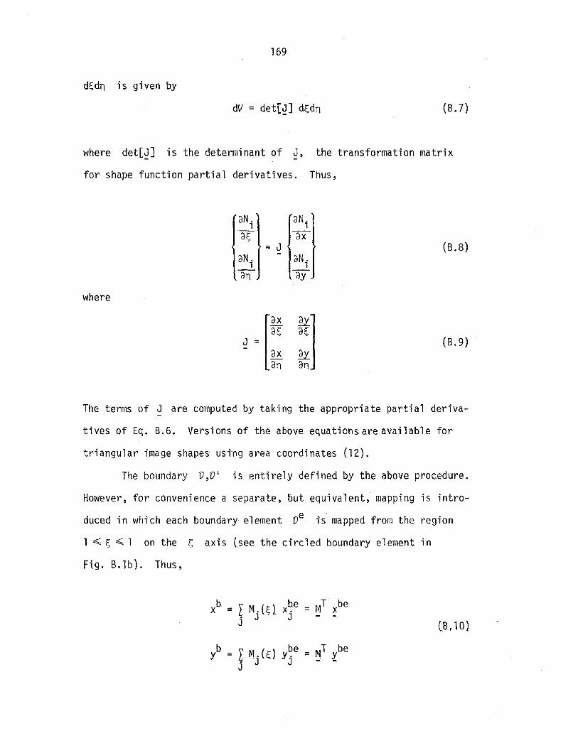
169

d~dn is given by

dV = det[~J d~dn (B.7)

where det[~J is the determinant of J, the transformation matrix

for shape function partial derivatives. Thus,

aN. aN.1 1

ar- ax= J (B.8)

aN. - aNi1

an ay

where

["X ~]a~ a~

J = (B.9)- ax Ex

on an

The terms of ~ are computed by taking the appropriate partial deriva

tives of Eq. B.6. Versions of the above equations are available for

triangular image shapes using area coordinates (12).

The boundary V,V' is entirely defined by the above procedure.

However, for convenience a separate, but equivalent, mapping is intro

duced in which each boundary element Ve is mapped from the region

1 ,,;; ~ ,,;; 1 on the ~ axi s (see the ci rc1ed boundary element in

Fig. B.lb). Thus,

C8, 1Q)

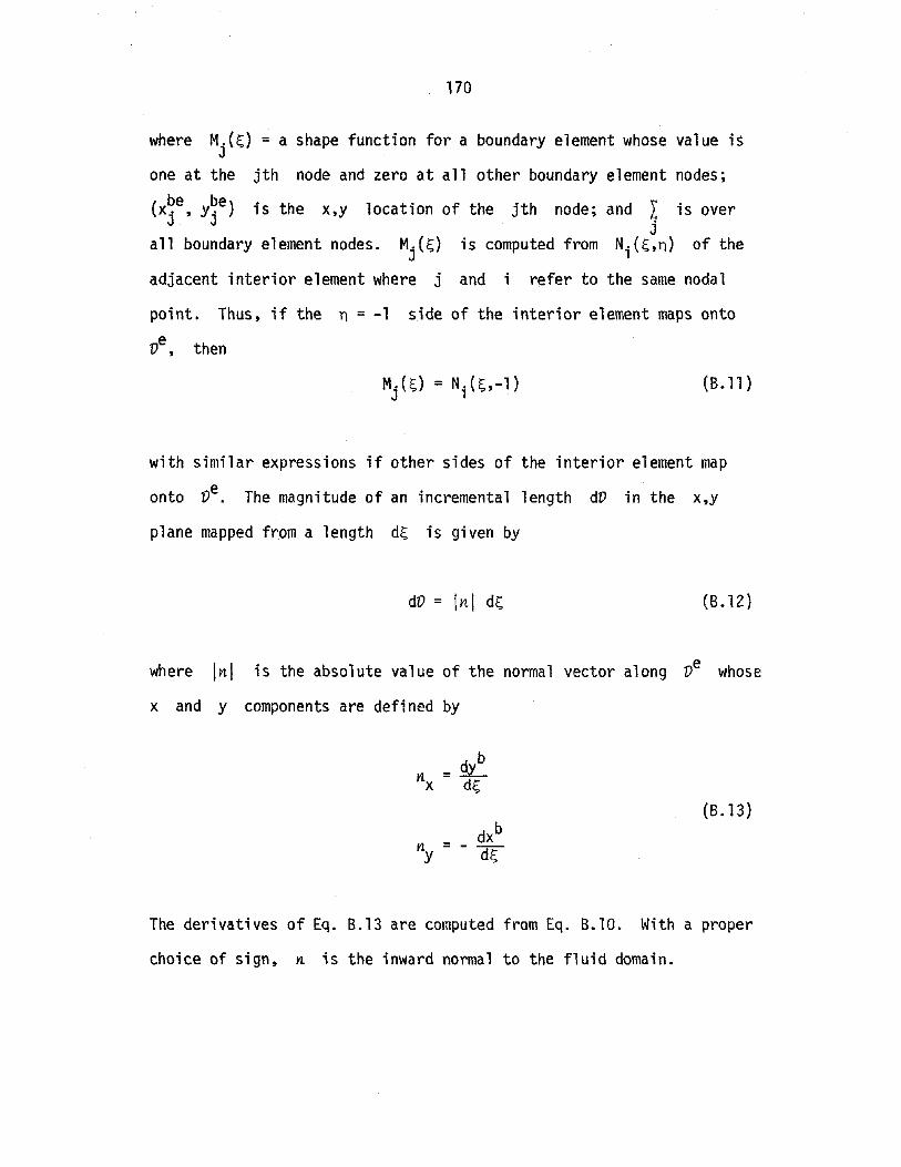
170

where M.(~) = a shape function for a boundary element whose value isJ

one at the jth node and zero at all other boundary element nodes;

(x~e, y~e) is the x,y location of the jth node; and I is overj

all boundary element nodes. Mj(~) is computed from Ni(~,n) of the

adjacent interior element where j and i refer to the same nodal

point. Thus, if the n = -1 side of the interior element maps onto

Ve , then

(B.ll)

with similar expressions if other sides of the interior element map

onto Ve. The magnitude of an incremental length dV in the x,y

plane mapped from a length d~ is given by

dV = 1111 d~ (B.12)

where 1111 is the absolute value of the normal vector along Ve whose

x and y components are defined by

(B.13)

11 =Y

The derivatives of Eq. B.13 are computed from Eq. B.10. With a proper

choice of sign, 11 is the inward normal to the fluid domain.

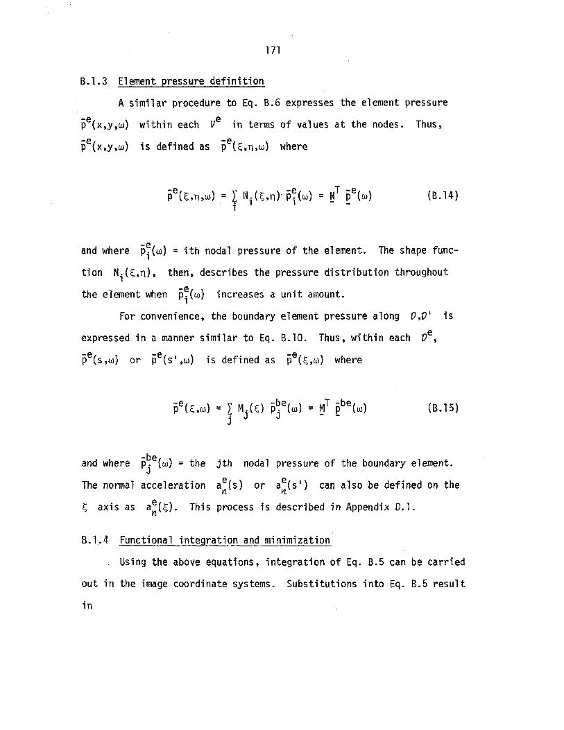
171

B.1.3 Element pressure definition

A similar procedure to Eq. B.6expresses the element pressure

pe(x,y,w) within each Ve in terms of values at the nodes. Thus,

pe(x,y,w) is defined as pe(~,n,w) where

(B.14)

-e )and where Pi(w = ith nodal pressure of the element. The shape func-

tion Ni{~,n), then, describes the pressure distribution throughout

-e( )the element when Pi w increases a unit amount.

For convenience, the boundary element pressure along V,V I is

expressed in a manner similar to Eq. B.10. Thus, within each Ve,

-e -e{)P (s,w) or p SI,W is defined as pe(~,w) where

(B.15)

-beand where Pj (w) = the jth nodal

The normal acceleration ae(s) or11

~ axis as a~(~). This process is

pressure of the boundary element.

ae(s') can also be defined on the11

described in Appendix 0.1.

B.1.4 Functional integration and minimization

Using the above equations, integration of Eq. B.5 can be carried

out in the image coordinate systems. Substitutions into Eq. 8.5 result

in

172

T [ 1+ J. {ebe(w)} iwq J

-1

(8.16)

where the shape function partial derivatives are computed by solving

Eq. B.8 for each node i of an element. The functional is now

approximate (denoted by -) because of the assumed interelement pressure

distributions. Equation B.16 is written as

where

1 1

f f (aN. aN. aN. aN.)H~. = ---'~ + ---'~ det[J] d~dn

, J _1 _1 ax ax ay ay -

(B.l7)

(B.18)1 1

G:·=f fN.N.det[J]dt,;dn'J -1 -1 ' J -

173

1D: = J

M. a~(~) Inl d~1 1-1

("B. 18) cont I d1

e J M. M. Inl d~B.. =lJ 1 J

-1

Symmetry of the element matrices is evident.

The matrices and vectors of Eq. B.17 can be assembled into a

single, larger set. In this process portions corresponding to the

nodes at the free surface a-c are not assembled because according to

Eq. B.3 the nodal pressures there are zero. Thus,

-(-) -()T [ w2

] - - T wX p = e w ~ + iwq ~ - C2 § e(w) - e(w) 9 Q (B. 19)

where the dimension of the vectors and symmetric matrices equals the

number of nodes below the free surface in Fig. B.lb. Minimization of

Eq. B.19 is carried out by setting the derivative with respect to each

Pi(w) to zero, resulting in

[2 ]. w· - w

~ + lwq ~ - C2 § p(w) =9 Q (B.20)

The non-zero portion of ~ is a submatrix corresponding to nodes

along V' where the boundary condition of Eq. B.2b is applied. D

has non-zero terms for only nodes along V,O' where accelerations are

applied.

174

B.2 One-Dimensional Fluid Domain

The fluid domain of Fig. B.2a arises as a cross-section of a

two-dimensional fluid domain when no variations in geometry or accel

erations are present in the x direction. The hydrodynamic pressure

p(y,w) is governed by the one-dimensional Helmholtz equation

2- 2d-n w~+-p=O

dy2 C2

subject to boundary conditions

dn w 1.. • - )dY (O.w) =- 9 ay + lwq p{O.w

p{H,w} = 0

The functional to be minimized is

(B.2l)

{B.22}

{B.23}

(8.24)

For a one-dimensional finite element discretization (Fig. B.2b), the

functional becomes a summation over the elements. Thus,

x(p) 1 .+ 2" lwq

(B.25)

175

a

y

b x

t.Oy

(a) FLUI D DOMAIN (b) FINITE ELEMENTDISCRETIZATION

FIG. B.2 ONE-DIMENSIONAL FINITE FLUID DOMAIN

176

where V is the domain a-b of the fluid.

Each element Ve is mapped onto the y axis from the region

-1 ~ ~ ~ 1 on the ~ axis (see the circled element in Fig. B.2b).

Thus,

y = I N.(~) y~ = NT ve• 1 1 - <l.1

(8.26)

where Ni(~) = shape function for the ith node; y~ is the y

location of the ith node; and L is over all element nodes. Thei

magnitude of an incremental length dy mapped from the length d~

is given by

dy=%td~ (B.27)

where the derivative is computed from Eq. B.26. Also,

dN. d dN._, = r:!1- _1 (B.28)d~ dE.: dy

The element pressure distribution ~e(y,w) is defined with ~e(~,w)

where

IN. (~) p~(w).' ,1

(B.29)

-eand where Pi(w) is the ith nodal pressure of the element.

Using the above equations, integration of Eq. B.25 can be

carried out in the ~ coordinate system. Substitutions into Eq. 8.25

result in

177

X(p) = ~ {ee(W)jT [~e _ ~~ §el ee(w) - ~.; p(O,w) +} iwq (p(O,w))2

(B.30)

where1

e J dN. dN. dH.. = __1 _J ~ de1J dy dy di; <,

-1(B.3l)

and where the shape function derivatives are found from Eq. B.28.

The matrices and vectors of Eq. B.30 can be assembled into a

single, larger set. The result, omitting portions corresponding to

the node at a to satisfy Eq. B.23, is

X(p) = e(w)T [~ - ~~ ~] e(w) - ~.~ Pk(w) +} iwq (Pk(w))2

(B.32)

where Pk{w) = p(O,w), and k corresponds to the node at b.

Minimization of Eq. B.32 is carried out by setting the derivative

with respect to each Pi(w) to zero, resulting in

rIf + iwq Bi - w2 rf] p(w) = ~ tf

too - C2 - - g -(B.33)

where Bi is a zero matrix except B~k = 1; and ~ is a zero vector

except ~ = a~. The matrices of Eq. B.33 are symmetric.

178

B.3 Three-Dimensional Fluid Domains

subject to boundary conditions along accelerating boundaries

(B.34)

~ (s ~r~w) = - W a (s r)9 YL ~(B.35a)

- ~ an(s I ~r'} + iwq pes I ,r l ,w) (B.35b)

and at the fluid free surface

(B.36)

In Eq. B.35, s~r are coordinates along the dam-fluid interface

a-b-c-d-a (denoted by V), and sl,r' are coordinates along the reser-

voir floor and sides b-f-i-j-g-c-b, a-e-i-f-b-a, and d-h-j-g-c-d

(denoted by V').

The functional to be minimized is

179

c

(a) FLUID DOMAIN

h

{b} FINITE ELEMENT DISCRETIZATION

FIG, B,3 THREE-DIMENSIONAL FINITE FLUID DOMAIN

(B.37)

180

J ~ an(s,r) p(s,r,w) dV + J } iwq (p(SI ,r l ,w))2 dV,

V,V I VI

s,r = s,r or s' ,r l

where V is the three-dimensional domain of the fluid. For the finite

element discretization of Fig. B.3b, the functional becomes a summation

over the elements. Thus

v11f ~a~(s,r) pe(s,r,w) dO + l f } iwq (pe(sl,r l ,w))2 dO,

Ve Ve

s,r = s,r or sl,r' (8.38)

B.3.2 Element mapping

Each finite element Ve is mapped into the x,y,z coordinate

system from a simple shape in an image coordinate system. For example,

the circled element of Fig. B.3b is mapped from the rectangular prism

1 ~ t;, ~ 1, 1 ~ n ~ 1, 1 < t; ~ 1 accord i ng to

181

x = ~ Ni(s~n~~) x~ = ~T ~e1

y = ~ Ni(s~n,~) y~ = ~T t e

1(B.39)

where Nl.(s,n~~) = shape function for the ith node; (x:~ y:, z:)111

is the x,y,z location of the ith node; and L is over all elementi

nodes. The magnitude of an incremental volume dV mapped from the

volume dsdnd~ is given byJ.

dV = det[~J dsdnd~ (BAD)

where

aN. aN.1 1

as ax

aNi aN.= J 1 (8.41)an ay

aN. aN.1 1

131;; az

and

ax ~ azas as at

J = ax ~ az (8.42)an I an an

ax ~ az01;; as o~

182

The terms of J can be computed from Eq.' B.39. Versions of the above

equations are available for triangular prism and tetrahedral image

shapes using area and volume coordinates (12).

The boundary V,V' is entirely defined by the above procedure.

For convenience, a separate but equivalent mapping is introduced in

which each boundary element Ve is mapped from a simple shape in an

image coordinate system. For example, the circled boundary element of

Fi g. B.3b is mapped from the rectangl e -1 ~ ~ ~. 1, -l~· n ~. 1

according to

(6.43)

b ~ M (~ ) zb.e = MT zbez = L • ""nj J J --

where M/~,n)= . shape function for the jth node of a boundary

( be be be) .element; x., y. ,z. 1S the x,y,z location of the jth node;J J J

and I is over all boundary element nodes. M·(~,n) is computedj J

from Ni(~,n,~) of the adjacent interior element where j and i

refer to the same nodal point. The magnitude of an incremental area

dV in the x,y,z system mapped from an area di;dn is given by

dV = Inl di;dn (B.44)

where Inl is the absolute value of the normal vector along ve

whose x, y, and z components are defined by

183

(8.45)

and where the partial derivatives are computed from Eq. 8.43. With a

proper choice of sign, n is the inward normal to the fluid domain.

B.3.3 Element pressure definition

Within each Ve the element pressure is defined as pe(~,n,1:;,w)

where

pe(~,n,1:;,w) = ~ Ni(~,n,1:;) p~(w) = ~T ee(w)1

(8.46)

-e( )and where Pi w = ith nodal pressure of the element.

distribution pe(s,r,w) or pe(sl,rl,w) along 0,0 1

is defined as pe(~,n,w) where

The pressure

within each Oe

(8.47)

and where p~e(w) = the jth nodal pressure of the boundary element.

The normal acceleration a~(s,r) or a~(sl,rl) can be defined as

ae(~,n) by the process described in Appendix D.2.n

(B.48)

184

B.3.4 Functional integration and minimization

Using the above equations, integration of Eq. B.38 can be car

ried out in the image coordinate systems. Thus,

x{p) = ~ {pe(wl}T [~e _~~ §el pe(w) - v.~, {pbe(w)jT ~ ~e

T+ L

I{Ebe(w)} iwq ~e Ebe(w)

V

where

111

H~j = f f f-1 -1 -1

(aN. aN. aN. aN. aN. aN.)

1 -l- 1 -.1 1-.1ax ax + ay ay + aT az det[~] dt;;dnds

1 1 1

G~j = J J J-1 -1 -1

N1. N. det[J] dt;;dnds

J -

(B.49)1 1

D~ = f J Mi a~(s,n) Ii'll dt;;dn-1 -1

M. t~. In I dt;; dn1 J

and where the shape function partial derivatives are computed by solv-

i ng Eq. B•41 .

The matrices and vectors of Eq. 8.48 can be assembled into a

single, larger set. The result, omitting portions corresponding to the

nodes at the free surface a-e-i-j-h-d-a, is

185

-(-) -{)T [ w2

] -{ -( T wX P = Ew ~ + iwq ~ - C2 § Ew) - Ew) 9 ~

Minimization of the functional X{p) leads to

(8.50)

(8.51)

The matrices of Eq. 8.51 are symmetric. The non-zero portion of § is

a submatrix corresponding to nodes along V', and D has non-zero

terms for only nodes along V,V'.

187Preceding page blank

APPENDIX C. BOUNDARY CONDITIONS FOR INFINITE FLUID DOMAINS

Figures C.1 and C.2 show infinite fluid domains of constant

depth and uniform cross-section, respectively. The two-dimensional

fluid domain of Fig. C.la is discretized into layers (Fig. C.1b), and

the three-dimensional fluid domain of Fig. C.2a is discretized into

channels (Fig. C.2b). Discrete forms of the acceleration boundary

conditions at x = a are derived below. Integrals of the final

matrix equations can be evaluated by Gauss quadrature.

C.l Infinite Fluid Domain of Constant Depth

The layer discretization in Fig. C.1b is defined by the one-

dimensional discretization along a-b, and thus the mapping process

of Sec. B.2 can be applied. Each one-dimensional element is mapped

onto the y axis from the region -1 ~ ~ ~ 1 on the ~ axis (see

the circled element in Fig. C.lb). Thus, from Eq. B.26,

y = ~T :l (C.l)

where ~T = vector of shape functions for an element; and t e=

coordinate vector for the element nodes. The pressure distribution

pe(x,y,w) within each layer is defined as pe(x,~,w) where

-e T -e( )p (x,~,w) = ~ p X,w (C.2)

-eand where E (x,w) = vector of pressures along nodal lines of a layer.

The normal acceleration on the x = 0 face of a layer a~(y) can also

188

0

f-4 1~l

V

- to,

---- b-

H .It

(0) FLUID DOMAIN (b) LAYER DISCRETIZATION

FIG. C.l INFINITE FLUID DOMAIN OF CONSTANT DEPTH

189

be defined on the ~ axis as a~(~).

The continuum boundary condition along the face a-b at x = 0

is given by

(C.3)

and within a layer by

(C.4)

According to Eq. B.18, the element vector of nodal accelerations is

found as

(C.5)

where ~ is computed from Eq. C.l. Substitution of Eq. C.2 into

Eq. C.4 and the result into Eq. C.5 yields

[

1 ] -e~ De = - I N NT ~ d~ d~ (O,w)9 - - - d~ dx

-1

Or, switching sides,

e dpe w e§ d-x (O,w) = - g Q

(C.6)

(C.7)

190

where

1e

J N. .Q1. (C.B)G•• = Nj d~ d~lJ 1

-1

Assembly for all elements along a-b results in

(C.9)

where the matrix ~ is the same one of Eq. B.33. Only equations for

nodes below the free surface node at a are included in Eq. C.9.

C.2 Infinite Fluid Domain of Uniform Cross-Section

The channel discretization in Fig. C.2b is defined by the two

dimensional discretization along a-b-c-d-a, and thus the mapping

procedure of Sec. B.l is applicable. Each two-dimensional element is

mapped onto the y,z plane from a simple shape in an image coordinate

system. For example, the circled element of Fig. C.2b is mapped from

the rectangle -1 ~ l; ~ 1, -1 ~ n ~ L Thus, from Eq. B.6,

(C.10)

where ~T = vector of shape functions for an element; and te,~e =

coordinate vectors for the element nodes. The pressure distribution

pe(x,y,z,w) within each channel is defined as pe(x,~,n,w) where

192

-pe(x ~ ) = ~T -Ee(x,w),,,,,n,w (C.ll)

and where ee(x,w) = vector of pressures along nodal lines of a channel.

The normal acceleration on the x = 0 face of a channel a~(y,z) is

defined as ae(~,n).xThe continuum boundary condition along the face a-b-c-d-a at

x = 0 is given by

~ (O,y,z,w) = - ~ ax(y,z)

and within a channel by

(C.12)

(C.l3)

According to Eq. B.49, the element vector of nodal accelerations is

found as

where

1 1

Qe = J I-1 -1

(C.14)

(C.15)

and where the partial derivatives are computed from Eq. C.10.

Substitution of Eq. C.ll into Eq. C.13 and the result into Eq. C.14

yields

193

-ee dQ _ .Y:!.- De (C.16)§ -ax (O,w) =

9 -

where

1 1e

f I N. N. 1ft I d~dn (C.l?)G•. =lJ 1 J x

-1 -1

Assembly for all elements within a-b-c-d-a results in

Gi ~djj (0,w) = - Y:!.- OX- X 9 -

where only equations for nodes below the fluid free surface are

included.

(C.18)


APPENDIX D. BOUNDARY COMPUTATIONS FOR FINITE FLUID DOMAINS

The fluid domains considered here are the two and three-

dimensional finite 'fluid domains of Figs. B.l and B.3. Computation of

the nodal acceleration vectors D~ and D. resulting from accelera--0 -J

tions of the ground in the direction ~ with rigid dam and accelera-

tions of the dam in its jth mode, respectively, is discussed. From

pressure vectors pf~(w) and p~(w) along the dam-fluid interface,-0 -J

computation of the hydrodynamic force vectors Qf~(w) and Q~(w) is-0 -J

also discussed. Vectors and matrices with superscript f contain

terms corresponding to all nodes along the dam-fluid interface.

Integrals of the final matrix equations can be evaluated by Gauss

quadrature.

D.l Two-Dimensional Fluid Domains

D.l.l Computation of Q~, ~ =x,y and Qj

Accelerating fluid boundaries in Fig. B.l include the dam-fluid

interface a-b and reservoir floor b-c, denoted by V and V' with

boundary coordinates sand Sl. These boundaries are located by a

mapping procedure described in Sec. B.l in which each boundary element

Ve is mapped from the region -1 ~ ~ ~ 1 on the ~ axis. Thus, from

Eq. B. 10,

(D.1)

196

where ~ =vector of shape functions for a boundary element; and

~be, ~be = coordinate vectors for the boundary element nodes. If a

boundary element Ve accelerates in the normal direction at a~(s)

or ae(s'), then from Eq. B.18 the element vector of nodal accelera-n

tions is found as

(0.2)

where a~(s) or a~(s') is defined on the ~ axis as a~(~); and

Inl is the absolute value of the normal vector along Ve whose x

and y components are given by Eq. B.13 as

(0.3)

n =y

and where the derivatives are computed from Eq. 0.1. With a proper

choice of sign, n is the inward normal.S/.,

The acceleration vector Po' S/., = x,y results from an accelera-

tion a (s) = €s/"(s), S = s,s' of the boundary V,V'. €s/"(s) orn

€s/"(s') defines the length of the component of a unit vector along s/.,

in the direction of the inward normal n. Within each Ve,

e nS/.,a (~) = "T::Tn I nl

(D.4)

197

and substitution into Eq. 0.2 yields

1

De = J~ n~ di;

-1

(0.5)

Assembly of each Qe over V,V'

from the free surface nodes.

forms D~.-0

No terms are assembled

D. results from an acceleration of V from the dam-fluid inter-J

face portion of the dam's jth mode ~I, whose x and y subvectors

are denoted by {¢~} and {¢~}. ane(s) is derived from the element-J x -J ysubvectors {¢~}x and {¢:} by

-J -J Y

(0.6)

Substitution of Eq. 0.6 into Eq. 0.2 yields

De = [fl MMT

n dS] {¢:} + [f1 MMTn dS] {¢:} (0.7)- -- x -J x -- Y -J Y

-1 -1

or

(0.8)

where

1

= I-1

198

M. M. 11 d~1 J x

(D.9)1

~ eJ - IB •• -. -y lJ-1

M. M. 11 d~1 J Y

Assembly of Eq. D.8 over V for each Ve yields

(D.10)

where Bf and Bf are symmetric matrices. D. is assembled from-x -y -J

terms of D~ corresponding to nodes below the free surface.-J

D. 1. 2 Computation of i{Q,(w), 51, =x,y and Q~ (w)-0 -J

Solution of Eq. B.20 with acceleration vector DQ, results in-0

the pressure vector pQ,(w). Along V, the pressure distribution-0

within Ve is pe(s,w), defined as pe(~,w) where, from Eq. B.15,

(D.11 )

199

I1X -e( ) I I d~ TnT p ~ ,w 11 ~ (0.12)


or

Assembly of Eq. 0.14 over V for each' Ve yields

{fi} f -f,Q,( )90 (w) x = ~x ~o w

and in like manner,

(0.13)

(D. 14)

(D. 15a)

(0.15b)

f f -f,Q,§x and §y of Eqs. 0.10 and 0.15 are the same, and ~o (w) lists

the terms of p,Q,(w) along the dam~fluid interface V and includes a-0

zero term for the surface node at a .. QH(w), ,Q, = x,y is assembled. -0-fi -Hfrom {90 (w)}x and {90 (w)}y of Eq. 0.15 and ordered to correspond

fto <p ••-J

and ordered to correspond to ~I.

The hydrodynamic terms of Eq.

200

Solution of Eq. B.20 with D. results in EJO(W), and the-J

vector pI(w) for pressures along V. g;(w) is assembled from the

subvectors

(0.16)

2.24 are of the form {~!}T Qf(w)-J -

and can be calculated in a direct manner. Premultiplication of Eq.. f T f TD.15a by {~j}x' Eq. D.15b by {~j}y' and addition of the resulting

equations yields

(0.17)

With use of Eq. 0.10,

= {DfolT .-H( )- J J eo w, Q, = x,y (D. 18a)

for the hydrodynami c added load terms. Simil arly,

for the hydrodynamic added mass terms.

(D.18b)

201

0.2 Three-Dimensional Fluid Domains

0.2.1 computation of DR" R,=x,y,z and D.-0 -J

Accelerating fluid boundaries in Fig. B.3 include the dam

fluid interface a-b-c-d-a (denoted by V with boundary coordinates

s,r) and the reservoir floor and sides b-f-i-j-g-c-b, a-e-i-f-b-a,

and d-h-j-g-c-d (denoted by V' with boundary coordinates s' ,r').

These boundaries are located by a mapping procedure described in

Sec. B.3 in which each boundary element is mapped from a simple shape

in an image coordinate system. For example, the circled boundary

element of Fig. B.3b is mapped from the rectangle -10::;;; t: 0::;;; 1,

-1 0::;;; n 0::;;; 1. Thus, from Eq. B. 43

xb = MT xbe

yb = ~T ¥,be

zb = MT zbe

(0.19)

where ~ = vector of boundary element shape functions; and

~be, lbe, ~be = coordinate vectors for the boundary element nodes. If

a boundary element Ve accelerates at a~(s,r) or a~(sl,rl), then

from Eq. B.49 the element vector of nodal accelerations is

1 1

De = J J~ a~(E:,n) 11'11 dt:dn-1 -1

(0.20)

wh~re ae(s,r) or ae(s',r ' ) is defined as a:(t:,n); and 11'11 isn n ,"

202

the absolute value of the normal vector along Ve where, from

Eq. B.45,

b b b bYr., = - ~ az _+ .2L~y an a~ a~ an (0.21)

With a proper choice of sign, n is the inward normal.t tQo' t=x,y,z results from an acceleration al1(s,r) = E: (s,r),

s,r = s,r or s',r l of the boundary 0,0'. Within each Oe,

(0.22)

and substitution into Eq. 0.20 yields

1 1

De = f f M '\ d~dn-1 -1

(0.23)

No terms are assembledformsAssembly of each Qe over 0,0'

from the free surface nodes.

OJ' results from an acceleration of V from ¢~ whose x, y,- ~

and z subvectors are den~ted by {~;}x' {~;}Y' and {~;}z·

a~(~,n) is derived from the element subvectors by

203

(0.24)

Substitution into Eq. D.20 yields

(0.25)

where

1 1

[~~]ij = f f M; M. Yl. dt;dnJ x-1 -1

1 1

[~~]ij = f f M. M. Yl.y dl;dn (D.26)1 J

-1 -1

1 1

[ e] f f M. M. Yl.z dl;dnB .. =-z lJ 1 J-1 -1

Assembly of Eq. D.25 over V for each Ve yields

D~ = Bf {~~} + B

f {~~} + Bf {~~}-J -x -J x -y -J Y -z -J Z

(0.27)

where Bf , Bf , and Bfz are symmetric matrices. D. is assembled-x -y - -J

from terms of D~ corresponding to nodes below the free surface.-J

2 2 . -fQ,( ) -f( )D.. Computatlon of Q w, R,=x,y,z and Q. w-0 -J

Solution of Eq. 6.51 with acceleration vector Q~ results in

the pressure vector e~(w). Along V, the pressure distribution within

204

ve is j)e(s,r,w} defined as j)e(i;,n,w} where, from Eq. B.47

-e( ) T -be( )p i;,n,w = ~ e w (0.28)

-beand where E (w) = vector of boundary element nodal pressures. The

x, y, and z subvectors of g~~(w} are denoted by {g~~(w)}x'

{Q_of~(w)}y and {Qf~(w)} and within Ve by {Qe(w}}, {Qe(w}},-0 z - x - y

and {ge(w}}z. By the method of virtual work

1 1

{ge(w)L = J f ~~pe(i;,n,w) In/ di;dn-1 -1


Assembly of Eq. 0.30 over V for each Ve yields

and in like manner

(0.29)

(0.30)

(0.31a)

(0.31b)

(D.3lc)

Bf , Bf and Bf of Eqs.-x -y -z1ists the terms of E~(w)

205

0.27 and 0.31 are the same, and pft(w)-0

along V and includes zero terms for-ftnodes at the free surface. go (w), t=x,y,z is assembled from the

component vectors of Eq. 0.31 and ordered to correspond to ~~. The-J

hydrodynamic added load terms of Eq. 2.24 can be found directly as

t = x,y,z (0.32a)

Solution of Eq. B.5l with o. results in PJ"(w), and the-J -

vector p~(w) for pressures along V. The hydrodynamic added mass-J

terms of Eq. 2.24 can be found as

(0. 32b)

207

APPENDIX E. CONTINUUM SOLUTION FOR THE INFINITEFLUID DOMAIN OF CONSTANT DEPTH

E.l First B.V.P.

The hydrodynamic pressure p(x,y,w) within the fluid domain of

Fig. E.la arises from an acceleration a (y) of the dam~fluid interxface a-b. The acceleration boundary condition at a-b is

By a separation of variables, p(x,y,w) is expressed as


2-d Px 2----:-z- K P = 0dx x

and Py(y,w) must satisfy

where K = separation constant; and

(Ll)

(E.2)

(E. 3a)

(E.3b)


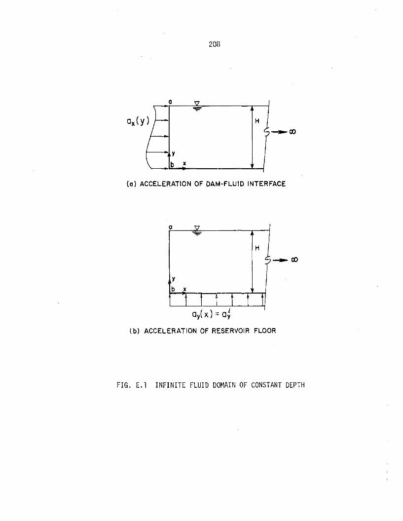
208

a

H

y

b l(

(0) ACCELERATION OF DAM-FLUID INTERFACE

a

H

Oy( X) :: a:

(b) ACCELERATION OF RESERVOIR FLOOR

FIG. E.1 INFINITE FLUID DOMAIN OF CONSTANT DEPTH

209

(E.4)

Boundary conditions for Eq. E.3b are

(E. 5a)

(E. 5b)

Equation E.3b together with the boundary conditions of Eq. E.5

defi nesan ei genva1ue problem. The nth ei genfuncti on is denoted by

~n(Y) and to satisfy Eq. E.3b must be of the form

(E.6)

where An is the nth eigenvalue. Equation E.5a imposes the condi

tion that

(E.7)

and substitution into Eq. E.6 with A (w) chosen as (A -wq)/2An n n

results in

(E.8)

210

Application of the boundary condition of Eq. E.5b leads to the trans-

cendental equation

2iA He n =

A - wqn (E.9)

from which the eigenvalues are computed.

The eigenfunctions ~n(Y) and eigenvalues An from Eqs. E.8

and E.9 are comp~ex valued and frequency dependent. The orthogonality

property of the eigenfunctions is summarized as

H

f ~n(Y) ~m(Y) dy =

o

H(A~ - w2q2) + iwq

2A2n

o if n'lm

if n=m

(L10)

The separated pressure function for the y coordinate is expressed as

(E.11)

The K in Eq. E.4 can now take on only the values given by

K = VA2- w

2= ~ + i vnn n C2 n

(E.12)

211

Since the infinite fluid domain is excited at x = O~ P (x,w) mustxdecay with increasing x or travel from x = 0 to x = 00. Thus, it

is of the form

-K xpx(x,w) = en, n = 1,2, ... (L13)

where the root with both ~n and vn positive is taken in computing

Kn from Eq. E.12. Combining the above expressions for Py(y,w) and

P (x,w) for all n leads tox

00 -K xp(x,y,w) = I nn(w) ~n(Y) e n

n=l(L14)

Substitution of Eq. E.14 into the boundary condition Eq. E.l

results in

(L15)

By multiplying Eq. E.15 by ~n(Y) and integrating from y = 0 to H

(using Eq. E.10), nn(w) is found as

leads to

dy. Substitution of Eq. L16 into Eq. E.14where

2A 2 I_ w n n- 9 (2 2 2) . KH A - w q + lwq nn

H

In = J ax(Y) ~n(Y)o

(E.16)

00

- W \'p(x,y,W) = -g. Ln=l

212

2A2 I -K Xn . n n2 2 2 ~ ~ (y) e

H(An - Wq ) + iwq n n(E.17)

p(x,y,w} is a bounded function of frequency and complex valued for

w > o.For q = 0, A = (2n-l}~/2H and ~ (y) = cos Ay (both realn n n

valued and frequency independent). Equation E.17 reduces to

2 00 I -K X- } w \' Ifl np(x,y,w = -g H L iZ- cos AnY e

n=l Ifl(E. 18)

H

where In = fax(y} cos AnY dye For w < AnC, Kn = ~n; and foro

w > AnC, Kn = ivn. Thus, ~n(Y} either decays exponentially with

-~ xincreasing x at e n (w < AnC) or is an undecaying harmonic

-iv xe n (w > AnC). Also, for an eigenfrequency w~ = AnC, Kn = 0

and the amplitude of ~n(Y} is infinite. The part of the amplitude

that approaches infinity is real below w~ and imaginary above.n .

E.2 Second B.V.P.

The problem of Fig. E.1b is one-dimensional in the y

coordinate. The hydrodynamic pressure p(y,w} arising from the

acceleration a~ of the reservoir floor is governed by the oney

dimensional Helmholtz equation:

213

subject to boundary conditions

~ (0) W i +. -(0 )dy ,w = - 9 ay lwq p ,w

p(H,w) = 0

The general solution to Eq. E.19 is

(E.19)

(E.20)

(E.2l)

wiCY

e (E. 22)

Application of the boundary conditions of Eqs. E.20 and E.21 and some

algebraic manipulation results in

wC i sinI(H-y)p(y,w) =-- a

g w Y cos I H + iCq sin fH (E.23)

p(y,w) can also be determined using an eigenfunction expansion

employing the complex valued and frequency dependent eigenvalues An

and eigenfunctions~n(Y) resulting from the associated eigenprob1em

of the first B.V.P. p(y,w) is expressed as

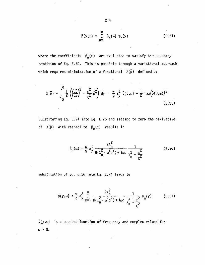
214

00

(E. 24)

where the coefficients B (00) are evaluated to satisfy the boundaryn

condition of Eq. E.20. This is possible through a variational approach

which requires minimization of a functional X(p) defined by

H

x(ji) = J0 ~ (($t -~~ ji2) dy • ~ a; ji(O,,,,} + ~ ;""1 (ji(O,,,,})2

(E.25)

Substituting Eq. E.24 into Eq. E.25 and setting to zero the derivative

of X(p) with respect to Bn(oo) results in

2. 2A 1

_ W a-L. n- 9 y H(A2 2 2) + . 2 2n - 00 q lwq A _ ~

n C2

Substitution of Eq. E.26 into Eq. E.24 leads to

(E. 26)

• 00

- W .(. \'p(y,oo) = - a Lg Y n=l

21..2n 12 2 2 . 2 1/Jn(y)

H(An - 00 q ) + iooq A2 ~ ~

n C2

(E.27)

p(y,w) is a bounded function of frequency and complex valued for

w > O.

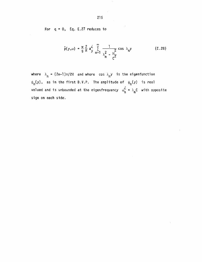
215

For q = 0, Eq. E.27 reduces to

(E. 28)

where An = (2n-1)n/2H and where cos AnY is the eigenfunction

~n{Y)' as in the first B.V.P. The amplitude of ~n{Y) is real

valued and is unbounded at the eigenfrequency w~ = AnC with opposite

sign on each side.

217

APPENDIX F. COMPUTATIONAL DETAILS

All computations of this report were carried out on a CDC 7600

computer with the Fortran program EAOFS (14). In this program, sub

space iteration (17), modified for consistent mass matrices (1), is

employed to solve the eigenproblem of the dam (Eq. 2.4/6.3) for the

first J natural frequencies w. and mode shapes ¢ ..J -J

The computer program can handle either finite fluid domains or

infinite fluid domains of irregular geometry through solution of

Eq. 3.6/7.6 of Eq. 3.39/7.26 wit~theaccelerations stated in Sees. 3.5

and 7.5. These equations are stored by a compacted, column-wise scheme

and solved by modified Crout reduction (18). If water compressibility

is included but fluid-foundation interaction neglected (q =0), then

the fluid domain equations have only real valued terms except in the

diagonal matrix ~ of Eq. 3.39/7.26 whose nth diagonal term K isn

imaginary if Arithmetic for complex valued numbers is used

only where necessary in solving Eq. 3.39/7.26. If fluid-foundation

interaction is included (q>O), then solutions to the fluid domain

equations are carried out entirely with complex arithmetic. The N

eigenvalues An and eigenvectors ~n of Eq. 3.39/7.26 are independent

of excitation frequency w if q = 0; in which case, they are deter-

mined from a single solution of the real-valued eigenproblem

Eq. 3.18/7.15 by the determinant search method (17). For q > 0, the

eigenproblem is frequency dependent and is complex valued except at

w = 0 where the above solution is applicable. The An and ~n at

successively higher frequencies are computed by inverse vector itera-

tion with shifting (19) using the An from the previous frequency to


218

compute the shifts and the previous ~n as trial vectors. The

incompressible water, rigid foundation solutions to Eq. 3.6/7.6 or

Eq. 3.39/7.26 are independent of excitation frequency; the compressi

ble water solution at w = 0 i~s employed.

Table F.1 lists the Central Processor times on the CDC 7600

to compute frequency response functions of J dam modes for the con

crete gravity dam with both the finite fluid domain and the infinite

fluid domain with sloped floor (Figs. 4.1b and c) and for symmetric

and antisymmetric cases of Morrow Point Dam with infinite fluid domain

(Fig. 8.1). If the reservoir is empty, then solution of the eigen

problem of the dam accounts for nearly all the computational effort.

C.P. times are 1ist~d in Table F.1a.

With compressible water, nearly all the computational effort is

spent to solve Eq. 3.6/7.6 or to solve Eq. 3.39/7.26 (along with the

eigenprob1em Eq. 3.18/7.15 if q> 0) for the range of excitation

frequencies. Average C.P. times per frequency, both neglecting and

including fluid-foundation interaction, are listed in Table F.1b. The

total C.P. times also listed are based on the numbers of frequencies

indicated which are sufficient to define the frequency response func

tions for J dam modes. Fewer frequencies are required when f1uid

foundation interaction is included because of the smoother response

curves.

From Table F.l, the total C.P. times when the reservoir is

empty are small compared to those when compressible water is included.

Solution times with incompressible water would also be small because

only one solution of the fluid domain equations is required. The

219

inclusion of fluid-foundation interaction increases the total computa

tional effort about 60% for the concrete gravity dam and about 600% for

Morrow Point Dam. The relatively large computational effort for Morrow

Point Dam when fluid-foundation interaction is included is due to the

time consuming solution of the complex valued, frequency dependent

eigenproblem Eq. 3.18/7.15 which accounts for most of the computational

effort.

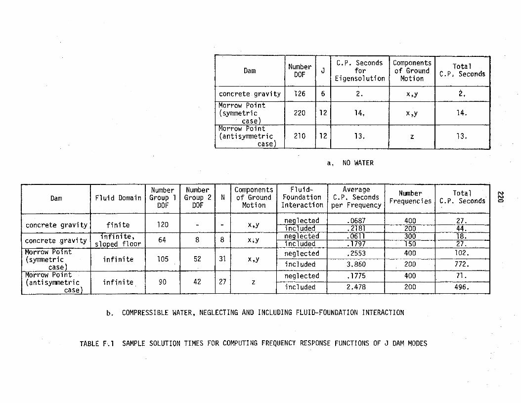
Number C.P. Seconds Components TotalDam DOF J for of Ground C.P. SecondsEigensolution Motion

concrete gravity 126 6 2. x,y 2.Morrow Point(symmetric 220 12 14. x,y 14.

case)Morrow Point(anti symmetric 210 12 13. z 13.

case)

a. NO WATER

Number Number Components F1uid- Average Number TotalDam Fluid Domain Group 1 Group 2 N of Ground Foundation C.P. Seconds Frequencies C.P. SecondsDOF DOF Motion Interaction per Frequency

neglected .0687 400 27.concrete gravity finite 120 - - x,y included .2181 200 44.infinite, 8 neqlected .0611 300 18.concrete gravity sloped floor 64 8 x,y included .1797 150 27.

Morrow Point neglected .2553 400 102.(symmetric i nfi nite 105 52 31 x,y

included 3.860 200 772.case)Morrow Point neglected .1775 400 71.(antiSymmetri~) i nfi ni te 90 42 27 z

included 2.478 200 496.case

b. COMPRESSIBLE WATER, NEGLECTING AND INCLUDING FLUID-FOUNDATION INTERACTION

TABLE F~' SAMPLE SOLUTION TIMES FOR COMPUTING FREQUENCY RESPONSE FUNCTIONS OF J DAM MODE~

N

~

221

EERC REPORT LISTING

223


EARTHQUAKE ENGINEERING RESEARCH CENTER REPORTS

NOTE: Numbers in parenthesis are Accession Numbers assigned by the National Technical Information Service: these arefollowed by a price code. Copies of the reports may be ordered from the National Technical Information Service, 5285Port Royal Road, Springfield, Virginia, 22161. Accession NUlnbers should be quoted on orders for reports (PB --- ---)and remittance must accompany each order. Reports without this information were not available at time of printing.Upon request, EERC will mail inquirers this information when it becomes available.

EERC 67-1

EERC 68-1

EERC 68-2

EERC 68-3

EERC 68-4

EERC 68-5

EERC 69-1

EERC 69-2

EERC 69-3

EERC 69-4

EERC 69-5

EERC 69-6

EERC 69-7

EERC 69-8

"Feasibility Study Large-Scale Earthquake Simulator Facility," by J. Penzien, J.G. Bouwkamp, R.W. Cloughand D. Rea - 1967 (PB 187 905)A07

Unassigned

"Inelastic Behavior of Beam-to-Column Subassemblages Under Repeated Loading," by V. V. Bertero - 1968(PB 184 888) A05

"A Graphical Method for Solving the Wave Reflection-Refraction Problem," by H.D. McNiven and Y. Mengi -1968(PB 187 943)A03

"Dynamic Properties of McKinley School Buildings," by D. Rea, J.G. Bouwkamp and R.W. Clough -1968(PB 187 902)A07

"Characteristics of Rock Motions During Earthquakes,lI by H.B. Seed, I.M. Idriss and F.W. Kiefer -1968(PB 188 338) A03

"Earthquake Engineering Research at Berkeley," - 1969 (PB 187 906)All

"Nonlinear Seismic Response of Earth Structures," by M. Dibaj and J. Penzien -1969 (PB 187 904)A08

"Probabilistic Study of the Behavior of Structures During Earthquakes," by R. Ruiz and J. Penzien -1969(PB 187 886}A06

"Numerical Solution of Boundary Value Problems in Structural Mechanics by Reduction to an Initial ValueFormulation," by N. Distefano and J. Schujman-1969 (PB 187 942)A02

"Dynamic Programming and the Solution of the Biharmonic Equation," by N. Distefano -1969 (PB 187 941}A03

"Stochastic Analysis of Offshore Tower Structures," by A.K. Malhotra and J. Penzien -1969 (PB 187 903)A09

"Rock Motion Accelerograms for High Magnitude Earthquakes," by H.B. Seed and I.M. Idriss - 1969 (PB 187 940) A02

"Structural Dynamics Testing Facilities at the University of California, Berkeley," by R.M. Stephen,J.G. Bouwkamp, R.l'l. Clough and J. Penzien -1969 (PB 189 1l1)A04

EERC 69-9 "Seismic Response of Soil Deposits Underlain by Sloping Rock Boundaries," by H. Dezfulian and H.B. Seed1969 (PB 189 114)A03

EERC 69-10 "Dynamic Stress Analysis of Axisymmetric Structures Under Arbitrary Loading," by S. Ghosh and E.L. Wilson1969 (PB 189 026)AIO

EERC 69-11 "Seismic Behavior of Multistory Frames Designed by Different Philosophies," by J.C. Anderson andV. V. Bertero - 1969 (PB 190 662)AIO

EERC 69-12 "Stiffness Degradation of Reinforcing Concrete Members Subjected to Cyclic Flexural Moments," byV. V. Bertero, B. Bresler and H. Ming Liao - 1969 (PB 202 942}A07

EERC 69-13 "Response of Non-Uniform Soil Deposits to Travelling Seismic Waves," by H. Dezfulian and H.B. Seed - 1969(PB 191 023)A03

EERC 69-14 "Damping Capacity of a Model Steel Structure," by D. Rea, R.W. Clough and J.G.Bouwkamp-1969 (PB190663)A06

EERC 69-15 "Influence of Local Soil Conditions on Building Damage Potential during Earthquakes," by H.B. Seed andI.M. Idriss - 1969 (PB 191 036)A03

EERC 69-16 "The Behavior of Sands Under Seismic Loading Conditions," by M.L. Silver and H.B. Seed -1969 (AD 714 982)A07

EERC 70-1 "Earthquake Response of Gravity Dams, U by A.K. Chopra - 1970 (AD 709 640)A03

EERC 70-2 "Relationships between Soil Conditions and Building Damage in the Caracas Earthquake of July 29, 1967," byH.B. Seed, LM. Idriss and H. Dezfulian -1970 (PB 195 762)A05

EERC 70-3 "Cyclic Loading of Full Size Steel Connections," by E.P. Popov and R.M. Stephen-1970 {PB 213 545)A04

EERC 70-4 "Seismic Analysis of the Charaima Building, Caraballeda, Venezuela," by Subcommittee of the SEAONC ResearchCommittee: V.V. Bertero, P.F. Fratessa, S.A. Mahin, J.H. Sexton, A.C. Scordelis, E.L. Wilson, L.A. Wyllie,H.B. Seed and J. Penzien, Chairman -1970 (PB 201 455)A06

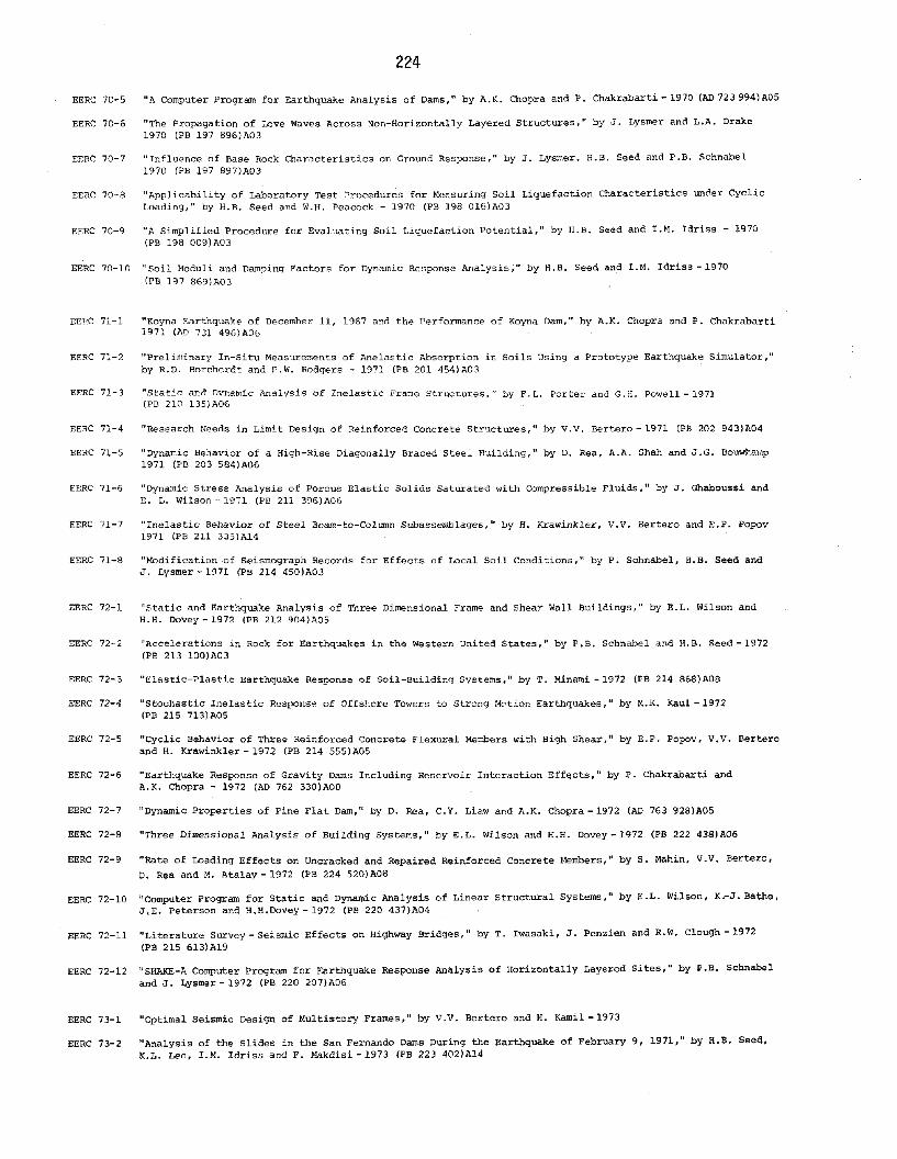
224

EERC 70-5 "A Computer Program for Earthquake Analysis of Dams," by A.K. Chopra and P. Chakrabarti -1970 (AD 723 994)A05

EERC 70-6 "The Propagation of Love Waves Across Non-Horizontally Layered Structures," by J. Lysmer and L.A. Drake1970 (Ps 197 896)A03

EERC 70-7 "Influence of Base Rock Characteristics on Ground Response," by J. Lysmer. H.B. Seed and P.B. Schnabel1970 (PB 197 897)A03

EERC 70-8 "Applicability of Laboratory Test Procedures for Measuring Soil Liquefaction Characteristics under CyclicLoading," by H.B. Seed and w.n. Peacock - 1970 (PB 198 016)A03

EERC 70-9 "A Simplified Procedure for Evaluating Soil Liquefaction Potential," by H.B. Seed and LM. Idriss - 1970(PB 198 009)A03

EERC 70-10 "Soil Moduli and Damping Factors for Dynamic Response Analysis;" by H.B. Seed and LM. Idriss -1970(PB 197 869)A03

EEEC 71-1 "Koyna Earthquake of December 11, 1967 and the Performance of Koyna Dam," by A.K. Chopra and P. Chakrabarti1971 (AD 731 496)AOG

EERC 71-2 "Preliminary In-Situ Measurements of Anelastic Absorption in Soils Using a Prototype Earthquake Simulator,"by R.D. Borcherdt and P.W. Rodgers - 1971 (PB 201 454)A03

EERC 71-3 "Static and Dvnamic Analysis of Inelastic Frame Structures," by F.L. Porter and G.H. Powell -1971(PS 210 135)A06

EERC 71-4 "Research Needs in Limit Design of Reinforced Concrete Structures," by V. V. Bertero - 1971 (PB 202 943)A04

EERC 71-5 "Dynamic Behavior of a High-Rise Diagonally Braced Steel Building," by D. Rea, A.A. Shah and J .G. Bouwr.m"p1971 (PB 203 584)A06

EERC 71-6 "Dynamic Stress Analysis of Porous Elastic Solids Saturated with compressible Fluids," by J. Ghaboussi andE. L. Wilson ··1971 (PB 211 396)A06

EERC 71-7 "Inelastic Behavior of Steel Beam-to-ColtBlln Subassenlblages," by H. Krawinkler, V.V. Bertero and E.P. Popov1971 (PB 211 335)A14

EERC 71-8 "Modification of Seismograph Records for Effects of Local Soil Conditions," by P. Schnabel, H.B. Seed andJ. Lysmer -1971 (PB 214 450)A03

EERC 72-1 "Static and Earthquake Analysis of Three Dimensional Frame and Shear Wall Buildings," by E.L. Wilson andH.H. Dovey -1972 (PB 212 904)A05

EERC 72-2 "Accelerations in Rock for Earthquakes in the Western United States," by P.B. Schnabel and H.B. Seed -1972(PB 213 100)A03

EERC 72-3 "Elastic-Plastic Earthquake Response of Soil-Building Systems," by T. Minami - 1972 (PB 214 868) A08

EERC 72-4 "Stochastic Inelastic Response of Offshore Towers to Strong Motion Earthquakes," by M.K. Kaul - 1972(PB 215 713)A05

EERC 72-5 "Cyclic Behavior of Three Reinforced Concrete Flexural Members with High Shear," by E.P. Popov, V.V. Berteroand H. Krawinkler - 1972 (PB 214 555)A05

EERC 72-6 "Earthquake Response of Gravity Dams Including Reservoir Interaction Effects," by P. Chakrabarti andA.K. Chopra - 1972 (AD 762 330)A08

EERC 72-7 "Dynamic Properties of Pine Flat Dam," by D. Rea, C. Y. Liaw and A.K. Chopra - 1972 (AD 763 928)A05

EERC 72-8 "Three Dimensional Analysis of Building Systems," by E.L. Wilson and H.H. Dovey -1972 (PE 222 438)A06

EERC 72-9 "Rate of Loading Effects on Uncracked and Repaired Reinforced Concrete Members," by S. Mahin, V.V. Bertero,

D. Rea and M. Atalay - 1972 (PB 224 520)A08

EERC 72-10 "Computer Program for Static and Dynamic Analysis of Linear Structural Systems," by E .L. Wilson, K.-J. Bathe,J.E. Peterson and H.H.,Dovey -1972 (PB 220 437)A04

EERC 72-11 "Literature Survey-Seismic Effects on Highway Bridges," by T. Iwasaki, J. Penzien and R.W. Clough-1972(PB 215 613)A19

EERC 72-12 "SHAKE-A Computer Program for Earthquake Response Analysis of Horizontally Layered Sites," by P.B. Schnabeland J. Lysmer - 1972 (PB 220 207)A06

EERC 73-1 "Optimal Seismic Design of Multistory Frames," by V.V. Bertero and H. Kam11-1973

EERC 73-2 "Analysis of the Slides in the San Fernando Dams During the Earthquake of February 9, 1971," by H.B. Seed,lCL. Lee, LM. Idriss and F. Makdisi -1973 (PE 223 402)A14

225

EERC 73-3 "Computer Aided Ultimate Load Design of Unbraced Multistory Steel Frames," by M.B. El-Hafez and G.H. Powell1973 (PB 248 315)A09

EERC 73-4 "Experimental Investigation into the Seismic Behavior of Critical Resions of Reinforced Concrete Componentsas Influenced by Moment and Shear," by M. Celebi and J. Penzien - 1973 (PB 215 884)A09

EERC 73-5 "Hysteretic Behavior of Epoxy-Repaired Reinforced Concrete Beams," by M. Celebi and J. Penzien - 1973(PB 239 568)A03

EERC 73-6 "General Purpose Computer Program for Inelastic Dynamic Response of Plane Structures," by A. Kanaan andG.H. Powell- 1973 (PB 221 260)A08

EERC 73-7 "A Computer Program for Earthquake Analysis of Gravity Dams Including Reservoir Interaction," byP. Chakrabarti and A.K. Chopra -1973 (AD 766 271)A04

EERC 73-8 "Behavior of Reinforced Concrete Deep Beam-Column Subassemblages Under Cyclic Loads," by O. Kiistu andJ.G. Bouwkamp -1973 (PB 246 117)A12

EERC 73-9 "Earthquake Analysis of Structure-Foundation Systems," by A. K. Vai sh and r,.K. Chopra - 1973 (AD 766 272) A07

EERC 73-10 "Deconvolution of Seismic Response for Linear Systems," by R.B. Reimer - 1973 (PB 227 179)A08

EERC 73-11 "SAP IV: A Structural Analysis Program for Static and Dynamic Response of Linear Systems," by K.-J. Bathe,E.L. Wilson and LE. Peterson -1973 (PB 221 967)A09

EERC 73-12 "Analytical Investigations of the Seismic Response of Long, Multiple Span Highway Bridges," by W.S. Tsengand J. Penzien-1973 (PB 227 816)AIO

EERC 73-13 "Earthquake Analysis of Multi-Story Buildings Including Foundation Interaction," by A.K. Chopra andJ.A. Gutip.rrez-1973 (PB 222 970)A03

EERC 73-14 "ADAP: A Computer Program for Static and Dynamic Analysis of Arch Darns," by R.W. Clough, J.M. Raphael andS. Mojtahedi - 1973 (PB 223 763)A09

EERC 73-15 "Cyclic Plastic Analysis of Structural Steel Joints," by R.B. Pinkney and R.W. Clough -1973 (PB226 843)A08

EERC 73-16 "Ql.'AD-4: A Computer Program for Evaluating the Seismic Response of Soil Structures by Variable DampingFinite Element Procedures," by I.M. Idriss, J. Lysmer, R. Hwang and H.B. Seed -1973 (PB 229 424)A05

EERC 73-17 "Dynamic :,,·havior of a Multi-Story Pyramid Shaped Building," by R.M. Stephen, J.P. Hollings andJ.G. Bouwkamp-1973 (PB 240 718)A06

EERC 73-18 "Effect of Different Types of Reinforcing on Seismic Behavior of Short Concrete Columns," by V.V. Bertero,J. Hollings, O. Kustu, R.M. Stephen and J.G. Bouwkamp -1973

EERC 73-19 "Olive View Medical Center Materials Studies, Phase I," by B. Bresler and V.V. Bertero -1973 (PB 235 986)A06

EERC 73-~0 "Linear and Nonlinear Seismic Analysis Computer Programs for Long MUltiple-Span ilighway Bridges," byW.S. Tseng and J. Penzien -1973

EERC 73-21 "Constitutive Models for Cyclic Plastic Deformation of Engineering Materials," by J.M. Kelly and P.P. Gillis1973 (PB 226 024)A03

EERC 73-22 "DRAIN - 2D User's Guide," by G.H. Powell-1973 (PB 227 016)A05

EERC 73-23 "Earthquake Engineering at Berkeley - 1973," (PB 226 033)All

EERC 73-24 Unassigned

EERC 73-25 "Earthquake Response of Axisymmetric Tower Structures Surrounded by Water," by C.Y. Liaw and A.K. Chopra1973 (AD 773 052)A09

EERC 73-26 "Investigation of the Failures of the Olive View Stairtowers During the San Fernando Earthquake and TheirImplications on Seismic Design," by V.V. Bertero and R.G. Collins -1973 (PB 235 106)A13

EERC 73-27 "Further Studies on Seismic Behavior of Steel Beam-Column Subassemblages," by V.V. Bertero, H. Krawinklerand E.P. Popov-1973 (PB 234 l72)A06

EERC 74-1 "Seismic Risk Analysis," by C.S. Oliveira -1974 (PB 235 920)A06

EERC 74-2 "Settlement and Liquefaction of Sands Under Multi-Directional Shaking," by R. Pyke, C.K. Chan and H.B. Seed1974

EERC 74-3 "Optimum Design of Earthquake Resistant Shear Buildings," by D. Ray, K.S. Pister and A.K. Chopra -1974(PB 231 172)A06

EERC 74-4 "LUSH - A Computer Program for Complex Response Analysis of Soil-Structure Systems," by J. Lysmer, T. Udaka,H.B. Seed and R. Hwang - 1974 (PB 236 796)A05

EERC 74-5

226

"Sensitivity Analysis for Hysteretic Dynamic Systems: Applications to Earthquake Engineering," by D. Ray1974 (PB 233 213)A06

EERC 74-6 "Soil Structure Interaction Analyses for Evaluating Seismic Response," by H.B. Seed, J. Lysmer and R. Hwang1974 (PB 236 519)A04

EERC 74-7 Unassigned

EERC 74-8 "Shaking Table Tests of a Steel Frame - A Progress Report," by R.W. Clough and D. Tang -1974 (PB 240 SE9)A03

EERC 74-9 "Hysteretic Behavior of Reinforced Concrete Flexural Members with Special Web Reinforcement," byV.V. Bertero, E.P. Popov and T.Y. Wang - 1974 (PB 236 797)A07

EERC 74-10 "Applications of Reliability-Based, Global Cost Optimization to Design of Earthquake Resistant Structures,"by E. Vitiello and K.S. Pister -1974 (PB 237 231)A06

EERC 74-11 "Liquefaction of Gravelly Soils Under Cyclic Loading Conditions," by R.T. Wong, H.B. Seed. and C.K. Chan1974 (PB 242 042)A03

EERC 74-12 "Site-Dependent Spectra for Earthquake-Resistant Design," by H.B. Seed, C. Ugas and J. Lysrner -1974(PB 240 953) A03

EERC 74-13 "Earthquake Simulator Study of a Reinforced Concrete Frame," by P. Hidalgo and R.W. Clough -1974(PB 241 9~4)A13

EERC 74-14 "Nonlinear Earthquake Response of Concrete Gravity Dams," by N. Pal -1974 (AD/A 006 583)A06

EERC 74-15 "Modeling and Identification in Nonlinear Structural Dynamics - I. One Degree of Freedom Models," byN. Distefano and A. Rath - 1974 (PB 241 548)A06

EERC 75-1 "Determination of Seismic Design Criteria for the Durnbarton Bridge Replacement Structure, Vol. I: Description,Theory and Analytical Modeling of Bridge and Parameters," by F. Baron and S. -H. Pang - 1975 (PB 259407)A15

EERC 75-2

EERC 75-3

EERC 75-4

EERC 75-5

EERC 75-6

"Determination of Seismic Design Criteria for the Durnbarton Bridge Replacement Structure, Vol. II: NumericalStudies and Establishment of Seismic Design Criteria," by F. Baron and S.-H. Pang -1975 (PB 259 408)All(For set of EERC 75-1 and 75-2 (PB 259 406»)

"Seismic Risk Analysis for a Site and a Metropolitan Area," by C.S. Oliveira -1975 (PB 248 l34)A09

"Analytical Investigations of Seismic Response of Short, Single or Multiple-Span Highway Bridges," byM. -C. Chen and J. Penzien - 1975 (PB 241 454) A09

"An Evaluation of Some Methods for Predicting Seismic Behavior of Reinforced Concrete Buildings," by S.A.Mahin and V.V. Bertero -1975 (PB 246 306)A16

"Earthquake SimUlator Study of a Steel Frame Structure, Vol. I: Experimental Results," by R.W. Clough andD.T. Tang -1975 (PB 243 981)A13

EERC 75-7 "Dynamic Properties of San Bernardino Intake Tower," by D. Rea, C.-Y. Liaw and A.K. Chopra-1975 (AD/A008406)AD5

EERC 75-8 "Seismic Studies of the Articulation for the Durnbarton Bridge Replacement Structure, Vol. I: Description,Theory and Analytical Modeling of Bridge Components," by F. Baron and R.E. Harnati-1975 (PB 251 539)A07

EERC 75-9 "Seismic Studies of the Articulation for the Durnbarton Bridge Replacement Structure, Vol. 2: NumericalStudies of Steel and Concrete Girder Alternates," by F. Baron and R.E. Hamati -1975 (PB 251 540)A10

EERC 75-10 "Static and Dynamic Analysis of Nonlinear Structures," by D.P. Mondkar and G.H. Powell -1975 (PB 242 434)A08

EERC 75-11 "Hysteretic Behavior of Steel Columns," by E.P. Popov, V.V. Bertero and S. Chandramouli-1975 (PB252 365)All

EERC 75-12 "Earthquake Engineering Research Center Library Printed Catalog," - 1975 (PB 243 711)A26

EERC 75-13 "Three Dimensional Analysis of Building Systems {Extended Version)," by E.L. Wilson, J.P. Hollings andH.H. Dovey - 1975 (PB 243 989)A07

EERC 75-14 "Determination of Soil Liquefaction Characteristics by Large-Scale Laboratory Tests," by P. De Alba,C.K. Chan and H.B. Seed -1975 (NUREG 0027)A08

EERC 75-15 "A Literature Survey - Compressive, Tensile, Bond and Shear Strength of Masonry," by R.L. Mayes and R.W.Clough - 1975 (PB 246 292)AIO

EERC 75-16 "Hysteretic Behavior of Ductile Moment Resisting Reinforced Concrete Frame Components," by V.V. Bertero andE.P. Popov - 1975 (PB 246 388)A05

EERC 75-17 "Relationships Between Maximum Acceleration, Maximum Velocity, Distance from Source, Local Site Conditionsfor Moderately Strong Earthquakes," by H.B. Seed, R. Murarka, J. Lysmer and LM. Idriss-1975 (PB 248 l72)A03

EERC 75-18 "The Effects of Method of Sample preparation on the Cyclic Stress-Strain Behavior of Sands," by J. Mulilis,C.K. Chan and H.B. Seed - 1975 (Summarized in EERC 75-28)

227

EERC 75-19 "The Seismic Behavior of Critical Regions of Reinforced Concrete Components as Influenced by Moment, Shearand Axial Force," by M. B. Atalay and J. Penzien - 1975 (PB 258 842)All

EERC 75-20 "Dynamic Properties of an Eleven Story Masonry Building," by R.M. Stephen, J.P. Hollings, J.G. Bouwkamp andD. Jurukovski - 1975 (PB 246 945)A04

EERC 75-21 "State-of-the-Art in Seismic Strength of Masonry - An Evaluation and Review," by R.L. Mayes and R.W. Clough

1975 (PB 249 040)A07

EERC 75-22 "Frequency Dependent Stiffness Matrices for Viscoelastic Half-Plane Foundations," by A.K. Chopra,p. Chakrabarti and G. Dasgupta - 1975 (pB 248 121) A07

EERC 75-23 "Hysteretic Behavior of Reinforced Concrete Framed Walls," by T.Y. Wong, V.V. Bertero and E.p. Popov-1975

EERC 75-24 "Testing Facility for Subassemblages of Frame-Wall Structural Systems," by V.V. Bertero, E.p. Popov andT. Endo - 1975

EERC 75-25 "Influence of Seismic History on the Liquefaction Characteristics of Sands," by H.B. Seed, K. Mori andC. K. Chan - 1975 (Summarized in EERC 75-28)

EERC 75-26 "The Generation and Dissipation of Pore Water Pressures during Soil LiquefaCtion," by H.B. Seed, 1'.1'. Martinand J. Lysmer - 1975 (PB 252 648)A03

EERC 75-27 "Identification of Research Needs for Improving Aseismic Design of Building Structures," by v. V. Bertero1975 (PB 248 136)A05

EERC 75-28 "Evaluation of Soil Liquefaction Potential during Earthquakes," by H.B. Seed, I. Arango and C.K. Chan - 1975(NUREG 0026)A13

EERC 75-29 "Representation of Irregular Stress Time Histories by Equivalent Uniform Stress Series in LiquefactionAnalyses," by H.B. Seed, LM. Idriss, F. Makdisi and N. Banerjee -1975 (PB 252 635)A03

EERC 75-30 "FLUSH - A Computer Program for Approximate 3-D Analysis of Soil-Structure Interaction Problems," byJ. Lysmer, T. Udaka, C.-F. Tsai and H.B. Seed -1975 (PB 259 332)A07

EERC 75-31 "ALUSH - A Computer Program for Seismic Response Analysis of Axisymmetric Soil-structure Systems," byE. Berger, J. Lysmer and H.B. Seed-1975

EERC 75-32 "TRIP and TRAVEL - Computer Programs for Soil-Structure Interaction Analysis with Horizontally TravellingWaves," by T. Udaka, ,To Lvsmer and 11.8. Seed -1975

EERC 75-33 "Predicting the Performance of Structures in Regions of High Seismicity," by J. Penzien - 1975 (PB 248 130)A03

EERC 75-34 "Efficient Finite Element Analysis of Seismic Structure - Soil - Direction," by J. Lysmer, H.B. Seed, T. Udaka,R. N. Hwang and C.-F. Tsai - 1975 (PB 253 570)A03

EERC 75-35 "The Dynamic Behavior of a First Story Girder of a Three-Story Steel Frame Subjected to Earthquake Loading,"by R.W. Clough and L.-Y. Li -1975 (PB 248 841)A05

EERC 75-36 "Earthquake Simulator Study of a Steel Frame Structure, Volume II -Analytical Results," by D.T. Tang -1975{PB 252 926)AIO

EERC 75-37 "ANSR-I General Purpose Computer Program for Analysis of Non-Linear Structural Response," by D.P. Mondkarand G.H. Powell -1975 (PB 252 386)A08

EERC 75-38 "Nonlinear Response Spectra for Probabilistic Seismic Design and Damage Assessment of Reinforced ConcreteStructures," by M. Murakami and J. Penzien-1975 (PB 259 530)A05

EERC 75-39 "Study of a Method of Feasible Directions for Optimal Elastic Design of Frame Structures Subjected to Earthquake Loading," by N.D. Walker and K.S. Pister-1975 (PB 257 781)A06

EERC 75-40 "An Alternative Representation of the Elastic-Viscoelastic Analogy," by G. Dasgupta and J.L. Sackman-1975(pB 252 173) AD3

EERC 75-41 "Effect of Multi-Directional Shaking on Liquefaction of Sands," by H.B. Seed, R. Pyke and G.R. Martin -1975(PB 258 781)A03

EERC 76-1 "Strength and Ductility Evaluation of Existing Low-Rise Reinforced Concrete Buildings - Screening Method," byT. Okada and B. Bresler - 1976 (pB 257 906)All

EERC 76-2 "Experimental and Analytical Studies on the Hysteretic Behavior of Reinforced Concrete Rectangular andT-Beams," by S.-Y.M. Ma, E.P. Popov and V.V. Bertero -1976 (PB 260 843)A12

EERC 76-3 "Dynamic Behavior of a Multistory Triangular-Shaped Building," by J. Petrovski, R.M. Stephen, E. Gartenbaumand J .G. Bouwkamp - 1976 (PB 273 279)A07

EERC 76-4 "Earthquake Induced Deformations of Earth Dams," by N. Serff, H.B. Seed, F.L Makdisi & C.-Y. Chang - 1976(pB 292 065)A08

228EERC 76-5 "Analysis and Design of Tube-Type Tall Building Structures," by H. de Clercq and G.H. Powell -1976 (PB 252220)

AlO

EERC 76-6 "Time and Frequency Domain Analysis of Three-Dimensiona 1 Ground Motions, San Fernando Earthquake," by T. Kuboand J. Penzien (PB 260 556)All

EERC 76-7 "Expected Performance of Uniform Building Code Design Masonry Structures," by R.L. Mayes, Y. Ornote, S.W. Chenand R. W. Clough - 1976 (PB 270 098)A05

EERC 76-8 "Cyclic Shear Tests of Masonry Piers, Volume 1 - Test Results," by R.L. Mayes, Y. Omote, R.W.Clough - 1976 (PB 264 424)A06

EERC 76-9 "A Substructure Method for Earthquake Analysis of Structure - Soil Interaction," by J.A. Gutierrez andA.K. Chopra- 1976 (PB 257 783)A08

EERC 76-10 "Stabilization of Potentially Liquefiable Sand Deposits using Gravel Drain Systems," by H.B. Seed andJ.R. Booker-1976 (PB 258 820)A04

EERC 76-11 "Influence of Design and Analysis Assumptions on Computed Inelastic Response of Moderately Tall Frames," byG.H. Powell and D.G. Row - 1976 (PB 271 409)A06

EERC 76-12 "Sensitivity Analysis for Hysteretic Dynamic Systems: Theory and Applications," by D. Ray, K.S. Pister andE. Polak - 1976 (PB 262 859)A04

EERC 76-13 "Coupled Lateral Torsional Response of Buildings to Ground Shaking," by C.L. Kan and A.K. Chopra 1976 (PB 257 907)A09

EERC 76-14 "Seismic Analyses of the Banco de America," by V.V. Bertero, S.A. Mahin and J.A. Hollings - 1976

EERC 76-15 "Reinforced Concrete Frame 2: Seismic Testing and Analytical Correlation," by R.W. Clough andJ. Gidwani - 1976 (PB 261 323)A08

EERC 76-16 "cyclic Shear Tests of Masonry Piers, Volume 2 - Analysis of Test Results," by R.L. Mayes, Y. Ornateand R.W. Clough - 1976

EERC 76-17 "Structural Steel Bracing Systems: Behavior Under Cyclic Loading," by E.P. Popov, K. Takanashi andC.W. Roeder ~ 1976 (PB 260 715)A05

EERC 76-18

EERC 76-19

EERC 76-20

EERC 76-21

EERC 76-22

EERC 76-23

EERC 76-24

EERC 76-25

EERC 76-26

EERC 76-27

EERC 76-28

EERC 76-29

EERC 76-30

EERC 76-31

EERC 76-32

"Experimental Model Studies on Seismic Response of High Curved Overcrossings," by D. Williams andW.G. Godden - 1976 (PB 269 548)A08

"Effects of Non-Unifonn Seismic Disturbances on the Durnbarton Bridge Replacement Structure," byF. Baron and R.E. Hamati - 1976 {PB 282 981)A16

"Investigation of the Inelastic Characteristics of a Single Story Steel Structure using SystemIdentification and Shaking Table Experiments," by V.C. Matzen and H.D. McNiven - 1976 (PB 258 453)A07

"Capacity of Columns with Splice Imperfections," by E.P. Popov, R.M. Stephen and R. Philbrick - 1976(PB 260 378)A04

"Response of the Olive View Hospital Main Building during the San Fernando Earthquake," by S. A. Mahin,V.V. Bertero, A.K. Chopra and R. Collins - 1976 (PB 271 425)A14

"A Study on the Major Factors Influencing the Strength of Masonry Prisms," by N.M. Mostaghel,R.L. Mayes, R. W. Clough and S.W. Chen - 1976 (Not published)

"GADFLEA - A Computer Program for the Analysis of Pore Pressure Generation and Dissipation duringcyclic or Earthquake Loading," by J.R. Booker, M.S. Rahman and H.B. Seed - 1976 (PB 263 947)A04

"Seismic Safety Evaluation of a RiC School Building," by B. Bresler and J. Axley - 1976

"Correlative Investigations on Theoretical and Experimental Dynamic Behavior of a Model BridgeStructure," by K. Kawashima and J. Penzien - 1976 (PB 263 388) All

"Earthquake Response of Coupled Shear Wall Buildings," by T. srichatrapimuk - 1976 (PB 265 157)A07

"Tensile Capacity of Partial Penetration Welds," by E.P. Popov and R.M. Stephen - 1976 (PB 262 899)A03

"Analysis and Design of Ntunerical Integration Methods in Structural Dynamics," by H.M. Hilber - 1976{PB 264 410)A06

"Contribution of a Floor System to the Dynamic Characteristics of Reinforced Concrete Buildings," byL.E. Malik and V.V. Bertero - 1976 (PB 272 247)A13

"The Effects of Seismic Disturbances on the Golden Gate Bridge," by F. Baron, M. Arikan and R.E. Hamati _1976 {PB 272 279)A09

"Infilled Frames in Earthquake Resistant Construction," by R.E. Klingner and V.V. Bertero - 1976(PB 265 892)A13

229UCB/EERC-77/01 "PLUSH - A Computer program for Probabilistic Finite Element Analysis of Seismic Soil-Structure Inter

action," by M.P. Ramo Organista, J. Lysmer and H.B. Seed - 1977

UCB/EERC-77/02 "Soil-structure Interaction Effects at the Humboldt Bay Power Plant in the Ferndale Earthquake of June7, 1975," by J.E. Valera, H.B. Seed, C.F. Tsai and J. Lysmer - 1977 (PB 265 795)A04

UCB/EERC-77/03 "Influence of Sample Disturbance on Sand Response to Cyclic Loading," by K. Mori, H.B. seed and C.K.Chan - 1977 (PB 267 352)A04

UCB/EERC-77/04 "Seismological Studies of Strong Motion Records," by J. Shoja-Taheri - 1977 (PB 269 655)AIO

UCB/EERC-77/05 "Testing Facility for Coupled-Shear Walls," by L. Li-Hyung, V.V. Bertero and E.P. Popov - 1977

UCB/EERC-77/06 "Developing Methodologies for Evaluating the Earthquake Safety of Existing Buildings," by No.1 -B. Bresler; No.2 - B. Bresler, T. Okada and D. Zisling; No.3 - T. Okada and B. Bresler; No.4 - V.V.Bertero and B. Bresler - 1977 (PB 267 354)A08

UCB/EERC-77/07 "A Literature Survey - Transverse Strength of Masonry Walls," by Y. Ornote, R.L. Mayes, S.W. Chen andR.W. Clough - 1977 (PB 277 933)A07

UCB/EERC-77/08 "DRAIN-TABS: A Computer Program for Inelastic Earthquake Response of Three Dimensional Buildings," byR. Guendelman-Israel and G.H. Powell - 1977 (PB 270 693)A07

UCB/EERC-77/09 "SUBWALL: A Special Purpose Finite Element Computer Program for Practical Elastic Analysis and Designof Structural Walls with Substructure Option," by D.Q. Le, H. Peterson and E.P. Popov - 1977(PB 270 567) A05

UCB/EERC-77/10 "Experimental Evaluation of Seismic Design Methods for Broad Cylindrical Tanks," by D.P. Clough(PB 272 280)A13

UCB/EERC-77/ll "Earthquake Engineering Research at Berkeley - 1976," - 1977 (PB 273 507)A09

UCB/EERC-77/l2 "Automated Design of Earthquake Resistant Multistory Steel Building Frames," by N.D. Walker, Jr. - 1977(PB 276 526)A09

UCB/EERC-77/13 "Concrete Confined by Rectangular Hoops Subjected to Axial Loads," by J. Vallenas, V.V. Bertero andE.P. Popov - 1977 (PB 275 165)A06

UCB/EERC-77/14 "Seismic Strain Induced in the Ground During Earthquakes," by Y. Sugimura - 1977 (PB 284 201)A04

UCB/EERC-77/15 "Bond Deterioration under Generalized Loading," by V.V. Bertero, E.P. Popov and S. Viwathanatepa - 1977

UCB/EERC-77/16 "Computer Aided Optimum Design of Ductile Reinforced Concrete Moment Resisting Frames," by S.W.Zagajeski and V.V. Bertero - 1977 (PB 280 137)A07

UCB/EERC-77/17 "Earthquake Simulation Testing of a Stepping Frame with Energy-Absorbing Devices," by J.M. Kelly andD.F. Tsztoo - 1977 (PB 273 506)A04

UCB/EERC-77/18 "Inelastic Behavior of Eccentrically Braced Steel Frames under Cyclic Loadings," by C.W. Roeder andE.P. Popov - 1977 (PB 275 526)A15

UCB/EERC-77/19 "A Simplified Procedure for Estimating Earthquake-Induced Deformations in Dams and Embankments," by F.I.Makdisi and H.B. Seed - 1977 (PB 276 820)A04

UCB/EERC-77/20 "The Performance of Earth Dams during Earthquakes," by H.B. Seed, F.I. Makdisi and P. de Alba - 1977(PB 276 821)A04

UCB/EERC-77/21 "Dynamic Plastic Analysis Using Stress Resultant Finite Element Formulation," by P. Lukkunapvasit andJ.M. Kelly - 1977 (PB 275 453)A04

UCB/EERC-77 /22 "Preliminary Experimental Study of Seismic Uplift of a Steel Frame," by R.W. Clough and A.A. Huckelbridge1977 (PB 278 769)A08

UCB/EERC-77/23 "Earthquake Simulator Tests of a Nine-Story Steel Frame with Columns Allowed to uplift," by A.A.Huckelbridge - 1977 (PB 277 944)A09

UCB/EERC-77/24 "Nonlinear Soil-Structure Interaction of Skew Highway Bridges," by M.-C. Chen and J. Penzien - 1977(PB 276 176)A07

UCB/EERC-77/25 "Seismic Analysis of an Offshore Structure Supported on Pile Foundations," by D.D.-N. Liou and J. Penzien1977 (PB 283 180)A06

UCB/EERC-77/26 "Dynamic Stiffness Matrices for Homogeneous Viscoelastic Half-Planes," by G. Dasgupta and A.K. Chopra 1977 (PB 279 654)A06

UCB/EERC-77/27 "A Practical Soft Story Earthquake Isolation System," by J.M. Kelly, J.M. Eidinger and C.J. Derham 1977 (PB 276 814)A07

UCB/EERC-77/28 "Seismic Safety of Existing Buildings and Incentives for Hazard Mitigation in San Francisco: An

Exploratory Study," by A.J. Meltsner - 1977 (PB 281 970)A05

UCB/EERC-77/29 "Dynamic Analysis of Electrohydraulic Shaking Tables," by D. Rea, S. Abedi-Hayati and Y. Takahashi1977 (PB 282 569)A04

UCB/EERC-77/30 "An Approach for Improving Seismic - Resistant Behavior of Reinforced Concrete Interior Joints," byB. Galunic, V.V. Bertero and E.P. popov - 1977 (PB 290 870)A06

UCB/EERC-78/01

UCB/EERC-78/02

UCB/EERC-78/03

UCB/EERC-78/04

UCB/EERC-78/05

UCB/EERC-78/06

UCB/EERC-78/07

UCB/EERC-78/08

UCB/EERC-78/09

UCB/EERC-78/10

UCB/EERC-78/11

UCB/EERC-78/12

UCB/EERC-78/13

UCB/EERC-78/14

UCB/EERC-78/15

UCB/EERC-78/16

UCB/EERC-78/17

UCB/EERC-78/18

UCB/EERC-78/19

UCB/EERC-78/20

UCB/EERC-78/21

UCB/EERC-78/22

UCB/EERC-78/23

UCB/EERC-78/24

UCB/EERC-78/25

UCB/EERC-78/26

UCB/EERC-78/27

UCB/EERC-78/28

UCB/EERC-78/29

230"The Development of Energy-Absorbing Devices for Aseismic Base Isolation systems," by J.M. Kelly andD.F. Tsztoo - 1978 (PB 284 978)A04

"Effect of Tensile Prestrain on the Cyclic Response of Structural Steel Connections, by J.G. Bouwkampand A. Mukhopadhyay - 1978

"Experimental Results of an Earthquake Isolation System using Natural Rubber Bearings," by J.M.Eidinger and J.M. Kelly - 1978 (PB 281 686)A04

"seismic Behavior of Tall Liquid Storage Tanks," by A. Niwa - 1978 (PB 284 017)A14

"Hysteretic Behavior of Reinforced Concrete Columns Subjected to High Axial and Cyclic Shear Forces,lIby S.W. Zagajeski, V.V. Bertero and J.G. Bouwkamp .. 1978 (PB 283 858)A13

"Inelastic Beam-Column Elements for the ANSR-I Program," by A. Riahi, D.G. Rowand G.H. Powell - 1978

"Studies of Structural Response to Earthquake Ground Hotion," by O.A. Lope,,; and A.K. Chopra - 1978(PB 282 790)A05

"A Laboratory Study of the Fluid-Structure Interaction of Submerged Tanks and Caissons in Earthquakes,"by R.C. Byrd - 1978 (PB 284 957)A08

"Model for Evaluating Damageability of Structures," by 1. Sakamoto and B. Bresler - 1978

"Seismic Performance of Nonstructural and Secondary Structural Elements," by 1. Sakamoto - 1978

"Mathematical r·\odelling of Hysteresis Loops for Reinforced Concrete Columns," by S. Nakata, T. Sprouland J. Penzien - 1978

"Damageability in Existing Buildings," by T. Blejwas and B. Bresler - 1978

"Dynamic Behavior of a Pedestal Base Multistory Building," by R.M. Stephen, E.L. Wilson, J.G. Bouwkampand M. Button - 1978 (PB 286 650)A08

lISeismic Response of Bridges - Case Studies,lI by R.A. Imbsen, V. Nutt and J. Penzien - 1978(PB 286 503)AIO

"A Substructure Technique for Nonlinear Static and Dynamic Analysis," by D.G. Row and G.H~ Powell 1978 (PB 288 077)AIO

"Seismic Risk Studies for San Francisco and for the Greater San Francisco Bay Area," by C.S. Oliveira 1978

"Strength of Timber Roof Connections Subjected to Cyclic Loads," by P. Gulkan, R.L. Mayes and R.W.Clough - 1978

"Response of K-Braced Steel Frame Models to Lateral Loads,lI by J.G. Bouwkamp, R.M .. Stephen andE.P. Popov - 1978

"Rational Design Methods for Light Equipment in St:ructures Subjected to Ground Motion," byJ.L. Sackman and J.M. Kelly - 1978 (PB 292 357)A04

"Testing of a Wind Restraint for Aseismic Base Isolation," by J.M. Kelly and D.E. Chitty - 1978(PB 292 833) A03

"APOLLO - A Computer Program for the Analysis of Pore Pressure Generation and Dissipation in HorizontalSand Layers During Cyclic or Earthquake Loading," by P.P. Martin and H.B. Seed - 1978 (PB 292 835)A04

"Optimal Design of an Earthquake Isolation System," by M.A. Bhatti, K.S. Pister and E. Polak - 1978(PB 294 735)A06

"MASH - A Computer Program for the Non-Linear Analysis of Vertically Propagating Shear Waves inHorizontally Layered Deposits," by P.P. Martin and H.B. Seed - 1978 (PB 293 101)A05

"Investigation of the Elastic Characteristics of a Three Story Steel Frame Using System Identification,"by I. Kaya and H.D. McNiven - 1978

"Investigation of the Nonlinear Characteristics of a Three-story Steel Frame Using SystemIdentification," by 1. Kaya and H.D. McNiven - 1978

"Studies of Strong Ground Motion in Taiwan," by Y.M. Hsiung, B.A. Bolt and J. Penzien - 1978

"Cyclic Loading Tests of Masonry Single Piers: Volume 1 - Height to Width Ratio of 2," by P.A. Hidalgo,R.L. Mayes, H.D. McNiven and R.W. Clough - 1978

"Cyclic Loading Tests of Masonry Single Piers: Volume 2 - Height to Width Ratio of I," by S.-W.J. Chen,P.A. Hidalgo, R.L. Mayes, R.W. Clough and H.D. McNiven - 1978

"Analytical Procedures in Soil Dynamics," by J. Lysmer - 1978

231

UCBjEERC-79jOl "Hysteretic Behavior of Lightweight Reinforced ConcreteBeam-Column Subassemblages," by B. Forzani, E.P. Popov,and V.V. Bertero - 1979

UCBjEERC-79j02 "The Development of a Mathematical Model to Predict theFlexural Response of Reinforced Concrete Beams to CyclicLoads, Using System J;.dentification," by J.F. Stanton andH.D. McNiven - 1979

UCBjEERC-79j03 "Linear and Nonlinear Earthquake Response of SimpleTorsionally Coupled Systems," by C.L. Kan andA.K. Chopra - 1979

UCBjEERC-79j04 "A Mathematical Model of Masonry for Predicting ItsLinear Seismic Response Characteristics," by Y. Mengiand H.D. McNiven - 1979

UCBjEERC-79j05 "Mechanical Behavior of Lightweight Concrete Confinedby Different Types of Lateral Reinforcement," byM.A. Manrique, V.V. Bertero and E.P. Popov - 1979

UCB/EERC-79/06 "Static Tilt Tests of a Tall Cylindrical Liquid StorageTank," by R.W. Clough and A. Niwa - 1979

UCB/EERC-79/07 "The Design of Steel Energy Absorbing Restrainers andTheir Incorporation Into Nuclear Power Plants forEnhanced Safety: Volume 1 - Summary Report," byP.N. Spencer, V.F. Zackay, and E.R. Parker - 1979

UCBjEERC-79/08 "The Design of Steel Energy Absorbing Restrainers andTheir Incorporation Into Nuclear Power Plants forEnhanced Safety: Volume 2 - The Development of Analysesfor Reactor System Piping," "Simple Systems" byM.C. Lee, J. Penzien, A.K. Chopra, and K. Suzuki"Complex Systems" by G.H. Powell, E.L. Wilson,R.W. Cloughand D.G. Row - 1979

UCB/EERC-79j09 "The Design of Steel Energy Absorbing Restrainers andTheir Incorporation Into Nuclear Power Plants forEnhanced Safety: Volume 3 - Evaluation of ComrnericalSteels," by W.S. Owen, R.t-i.N. pe11oux, R.O. Ritchie,M. Fara1, T. Ohhashi, J. Top1osky, S.J. Hartman, V.F.Zackay, and E.R. Parker - 1979

UCB/EERC-79jlO "The Design of Steel E~ergy Absorbing Restrainers andTheir Incorporation Into Nuclear Power Plants forEnhanced Safety: Volume 4 - A Review of Energy-AbsorbingDevices," by J.M. Kelly and M.S. Skinner - 1979

UCB/EERC-79/ll "Conservatism In Summation Rules for Closely SpacedModes," by J.M. Kelly and J.L. Sackman - 1979

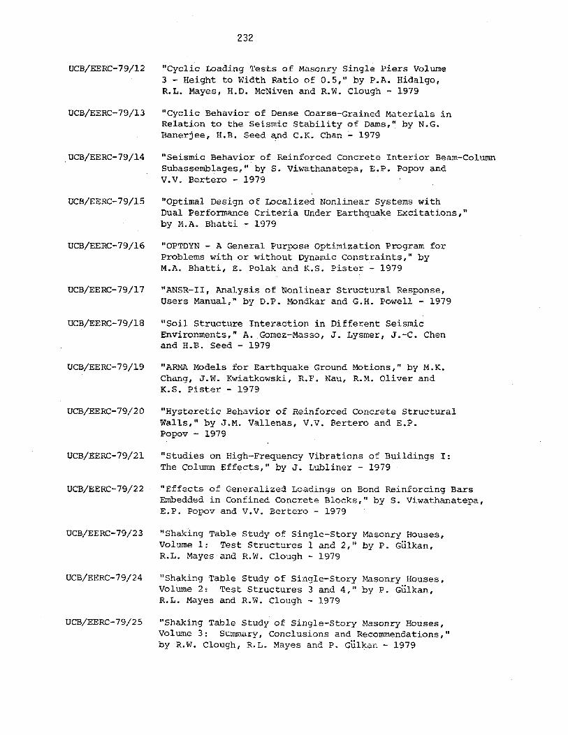
232

UCB/EERC-79/l2 I'Cyclic Loading Tests of Masonry Single Piers Volume3 - Height to Width Ratio of 0.5," by P.A. Hidalgo,R.L. Mayes, H.D. McNiven and R.W. Clough - 1979

UCB/EERC-79/l3 "Cyclic Behavior of Dense Coarse-Grained Materials inRelation to the Seismic Stability of Dams," by N.G.Banerjee, H.B. Seed ~nd C.K. Chan - 1979

UCB/EERC-79/l4 "Seismic Behavior of Reinforced Concrete Interior Beam-ColumnSubassemblages," by S. Viwathanatepa, E.P. Popov andV.V. Bertero - 1979

UCB/EERC-79/l5 "Optimal Design of Localized Nonlinear Systems withDual Performance Criteria Under Earthquake Excitations,"by M.A. Bhatti - 1979

UCB/EERC-79/l6 "OPTDYN - A General Purpose Optimization Program forProblems with or without Dynamic Constraints," byM.A. Bhatti, E. Polak and K.S. Pister - 1979

UCB/EERC-79/l7 "ANSR-II, Analysis of Nonlinear Structural Response,Users Manual," by D.P. Mondkar and G.H. Powell - 1979

UCB/EERC-79/18 "Soil Structure Interaction in Different SeismicEnvironments," A. Gomez-Masso, J. Lysmer, J.-C. Chenand H.B. Seed - 1979

UCB/EERC-79/19 "ARMA Models for Earthquake Ground Motions," by M.K.Chang, J.W. Kwiatkowski, R.F. Nau, R.M. Oliver andK.S. Pister - 1979

UCB/EERC-79/20 "Hysteretic Behavior of Reinforced Concrete StructuralWalls," by J.M. Vallenas, V.V. Bertero and E.P.Popov - 1979

UCB/EERC-79/21 "Studies on High-Frequency Vibrations of Buildings I:The Column Effects," by J. Lubliner - 1979

UCB/EERC-79/22 "Effects of Generalized Lo,3.dings on Bond Reinforcing BarsEmbedded in Confined Concrete Blocks," by S. Viwathanatepa,E.P. Popov and V.V. Bertero - 1979

UCB/EERC-79/23 "Shaking Table Study of Single-Story Masonry Houses,Volume 1: Test Structures 1 and 2," by P. Gulkan,R.L. Mayes and R.W. Clough - 1979

UCB/EERC-79/24 "Shaking Table Study of Single-Story ~~sonry Houses,Volume 2: Test Structures 3 and 4," by P. Giilkan,R.L. Mayes and R.W. Clough - 1979

UCB/EERC-79/25 "Shaking Table Study of Single-Story Masonry Houses,Volume 3: Summary, Conclusions and Recommendations,"by R.W. Clough, R.L. Mayes and P. Gulkan - 1979

233

UCB/EERC-79/26 "Reconunendations for a U.S.-Japan Cooperative ResearchProgram utilizing Large-Scale Testing Facilities," byU.S.-Japan Planning Group - 1979

UCB/EERC-79/27 "Earthquake-Induced Liquefaction Near Lake Amatitlan,Guatemala," by H.B. Seed, I. Arango, C.K. Chan,A. Gomez-Masso and R. Grant de Ascoli - 1979

UCB/EERC-79/28 "Infill Panels: Their Influence on Seismic Response ofBuildings," by J.W. Axley and V.V. Bertero - 1979

UCB/EERC-79/29 "3D Truss Bar Element (Type 1) for the ANSR-II Program,"by D.P. Mondkar and G.H. Powell - 1979

UCB/EERC-79/30 "2D Beam-Column Element (Type 5 - Parallel ElementTheory) for the ANSR-II Program," by D.G. Row, G.H. Powelland D. P. Mondkar

UCB/EERC-79/31 "3D Beam-Column Element (Type 2 - Parallel ElementTheory) for the ANSR-II Program," by A. Riahi, G.H. Powelland D.P. Mondkar - 1979

UCB/EERC-79/32 "On Response of Structures to Stationary Excitation," byA. Der Kiureghian - 1979

UCB/EERC-79/33 "Undisturbed Sampling and Cyclic Load Testing of Sands,"by S. Singh, H.B. Seed and C.K. Chan - 1979

UCB/EERC-79/34 "Interaction Effects of Simultaneous Torsional andCompressional Cyclic Loading of Sand," by P.H. Griffinand W.N. Houston - 1979

UCB/EERC-80/01 "Earthquake Response of Concrete Gravity Dams IncludingHydrodynamic and Foundation Interaction Effects," byA.K. Chopra, P. Chakrabarti and S. Gupta - 1980

UCB/EERC-80/02 "Rocking Response of Rigid Blocks to Earthquakes,"by C.S. Yim, A.K. Chopra and J. Penzien - 1980

UCB/EERC-80/03 "Optimum Inelastic Design of Seismic-Resistant ReinforcedConcrete Frame structures," by S.W. Zagajeski and V.V.Bertero - 1980

UCB/EERC-80/04 "Effects of Amount and Arrangement of Wall-PanelReinforcement on Hysteretic Behavior of ReinforcedConcrete Walls," by R. Iliya and V.V. Bertero - 1980

UCB/EERC-80/0S "Shaking Table Research on Concrete Dam Models," byA. Niwa and R.W. Clough - 1980

UCB/EERC-80/06 "piping with Energy Absorbing Restrainers: ParameterStudy on Small Systems," by G.H. Powell, C. Oughourlianand J. Simons - 1980

234

UCB/EERC-80/07 "Inelastic Torsional Response of Structures Subjectedto Earthquake Ground Motions," by Y. Yamazaki - 1980

UCB/EERC-80/08 "Study of X-Braced Steel Frame Structures UnderEarthquake Simulation," by Y. Ghanaat - 1980

UCB/EERC-80/09 "Hybrid Modelling of Soil-Structure "Interaction," byS. Gupta, T.W. Lin, J. Penzien and C.S. Yeh - 1980

UCB/EERC-80/10 "General Applicability of a. Nonlinear Model of a OneStory Steel Frame," by B.I. Sveinsson and H. l1cNiven - 1980

UCB/EERC-80/11 "A Green-Function Method for Wave Interaction with aSubmerged Body," by W. Kioka - 1980

UCB/EERC-80/12 "Hydrodynamic Pressure and Added Mass for AxiSYmmetricBodies," by F. Ni1rat - 1980

UCB/EERC-80/13 "Treatment of Non-Linear Drag Forces Acting on OffshorePlatforms," by B. V. Dao and J. Penzien - 1980

UCB/EERC-80/14 "2D Plane/Axisymmetric Solid Element (Type 3 - Elasticor Elastic-Perfectly Plastic) for the ANSR-II Program,"by D.P. Mondkar and G.H. Powell - 1980

UCB/EERC-80/15 "A Response Spectrum Method for Random Vibrations," byA. Der Kiureghian - 1980

UCB/EERC-80/16 "Cyclic Inelastic Buckling of Tubular Steel Braces," byV.A. Zayas, E.P. Popov and S.A. Mahin - June 1980

UCB/EERC-80/17 "Dynamic Response of Simple Arch Dams Including HydrodynamicInteraction," by C.S. Porter and A.K. Chopra - JUly 1980

UCB/EERC-80/18 "Experimental Testing of a Friction Damped AseismicBase Isolation System with Fail-Safe Characteristics,"by J.M. Kelly, K.B. Beucke and M.S. Skinner - July 1980

UCB/EERC-80/l9 "The Design of Steel Energy-Absorbing Restrainers and theirIncorporation into Nuclear Power Plants for Enhanced Safety(Vol lB): Stochastic Seismic Analyses of Nuclear Power PlantStructures and Piping Systems Subjected to Multiple SupportExcitations," by M.C. Lee a.nd J. Penzien - 1980

UCB/EERC-80/20 "The Design of Steel Ener~j-AbsorbingRestrainers and theirIncorporation into Nuclear Power Plants for Enhanced Safety(Vol lC): Numerical Method for Dynamic Substructure Analysis,"by J.M. Dickens and E.L. Wilson - 1980

UCB/EERC-80/2l "The Design of Steel Energy-Absorbing Restrainers and theirIncorporation into Nuclear Power Plants for Enhanced Safety(Vol 2): Development and Testing of Restraints for NuclearPiping Systems," by J.M. Kelly and M.S. Skinner - 1980

UCB/EERC-80/22

UCB/EERC-80/23

UCB/EERC-80/24

UCB/EERC-80/25

UCB/EERC-80/26

UCB/EERC-80/27

UCB/EERC-80/28

UCB/EERC-80/29

UCB/EERC-80/30

UCB/EERC-80/3l

UCB/EERC-80/32

UCB/EERC-80/33

UCB/EERC-80/34

235

"3D Solid Element (Type 4-Elastic or Elastic-PerfectlyPlastic) for the ANSR-II program," by D.P. Mondkar andG.H. Powell - 1980

"Gap-Friction Element (Type 5) for the ANSR-II Program,"by D.P. Mondkar and G.H. Powell - 19~0

flU-Bar Restraint Element (Type 11) for the ANSR-IIProgram," C. Oughourlian and G.H. Powell - 1980

"Testing of a Natural Rubber Base Isolation System byan Explosively Simulated Earthquake," by J.M. Kelly1980

"Input Identification from Structural VibrationalResponse," by Y. Hu - 1980

"Cyclic Inelastic Behavior of Steel Offshore Structures,"by V.A. Zayas, S.A. Mahin and E.P. Popov - 1980

"Shaking Table Testing of a Reinforced Concrete Framewith Biaxial Response," M.G. Oliva and R.W. Clough1980

"Dynamic Properties of a Twelve-Story Prefabricated PanelBuilding," by J .G. Bouwkamp, J.P. Kollegger andR.M. Stephen - 1980

"Dynamic Properties of a Eight-Story Prefabricated PanelBuilding," by J.G. Bouwkamp, J.P. Kollegger andR.M. Stephen - 1980

"Predictive Dynamic Response of Panel Type StructuresUnder Earthquakes,". by J.P. Kollegger and J.G. Bouwkamp1980

"The Design of Steel Energy-Absorbing Restrainers andtheir Incorporation into Nuclear Power Plants forEnhanced Safety: Vol 3, Testing of Commercial Steels inLow-Cycle Torsional Fatigue," by P. Spencer, E.R. Parker,E. Jongewaard and M. Drory - 1980

"The Design of Steel Energy-Absorbing Restrainers andtheir Incorporation into Nuclear Power Plants forEnhanced Safety: Vol 4, Shaking Table Tests of PipingSystems with Energy-Absorbing Restrainers," byS.F. Stiemer and W.G. Godden - 1980

"The Design of Steel Energy-Absorbing Restrainers andtheir Incorporation into Nuclear Power Plants forEnhanced Safety: Vol 5, Summary Report," by P. Spencer1980

236

UCB/EERC-80/35 "Experimental Testing of an Energy Absorbing BaseIsolation System," by J. Kelly, M.S. Skinner andK.E. Beucke - 1980

UCB/EERC-80/36 "Simulating and Analyzing Artificial Non-StationaryEarthquake Ground Motions," by R.F. Nau, R.M. Oliverand K.S. Pister - 19~O

UCB/EERC-80/37 "Stochastic Seismic Analysis of Nuclear Power PlantStructures and Piping Systems Subjected to MultipleSupport Excita,.tions," by M.C. Lee and J. Penziel) - 1980

UCB/EERC-80/38 "Inelastic Seismic Analysis of Large Panel Buildings,"by V. Schricker and G.H .. Powell - 1980

UCB/EERC-80/39 "Dynamic Response of Embankment, Concrete-Gravityand Arch Dams InclUding Hydrodynamic Interaction,"by J.F. Hall and A.K. Chopra - 1980

GRAVITY AND ARCH DAMS INCLUDING HYDRODYNAMIC ...

Documents

Transcript of GRAVITY AND ARCH DAMS INCLUDING HYDRODYNAMIC ...