University of Pennsylvania University of Pennsylvania

ScholarlyCommons ScholarlyCommons

Departmental Papers (MEAM) Department of Mechanical Engineering & Applied Mechanics

May 2005

Magneto-hydrodynamic Stirrer for Stationary and Moving Fluids Magneto-hydrodynamic Stirrer for Stationary and Moving Fluids

Shizhi Qian University of Pennsylvania

Haim H. Bau University of Pennsylvania, bau@seas.upenn.edu

Follow this and additional works at: https://repository.upenn.edu/meam_papers

Recommended Citation Recommended Citation Qian, Shizhi and Bau, Haim H., "Magneto-hydrodynamic Stirrer for Stationary and Moving Fluids" (2005). Departmental Papers (MEAM). 69. https://repository.upenn.edu/meam_papers/69

Postprint version. Published in Sensors and Actuators B: Chemical, Volume 106, Issue 2, May 13, 2005, pages 859-870. Publisher URL: http://dx.doi.org/10.1016/j.snb.2004.07.011

This paper is posted at ScholarlyCommons. https://repository.upenn.edu/meam_papers/69 For more information, please contact repository@pobox.upenn.edu.

Magneto-hydrodynamic Stirrer for Stationary and Moving Fluids Magneto-hydrodynamic Stirrer for Stationary and Moving Fluids

Abstract Abstract A magneto-hydrodynamic (MHD) stirrer that exhibits chaotic advection is designed, modeled, and tested. The stirrer can operate as a stand-alone component or it can be incorporated into a MHD-controlled network. The stirrer consists of a conduit equipped with individually controlled electrodes positioned along its opposing walls. The conduit is filled with an electrolyte solution and positioned in a uniform magnetic field. When a potential difference is applied across pairs or groups of electrodes, the resulting current interacts with the magnetic field to induce Lorentz forces and fluid motion. When the potential difference is applied across opposing electrodes that face each other, the fluid is propelled along the conduit’s length. When the potential difference is applied across diagonally positioned electrodes, a circulatory motion results. When the potential difference alternates periodically across two or more such configurations, chaotic motion evolves and efficient mixing is obtained. This device can serve as both a stirrer and a pump. The advantage of this device over previous designs of MHD stirrers is that it does not require electrodes positioned away from the conduit’s walls. Since this device has no moving parts, the concept is especially suitable for microfluidic applications.

Keywords Keywords Microfluidics, magneto-hydrodynamics (MHD), chaotic stirrer, microreactors, lab on a chip

Comments Comments Postprint version. Published in Sensors and Actuators B: Chemical, Volume 106, Issue 2, May 13, 2005, pages 859-870. Publisher URL: http://dx.doi.org/10.1016/j.snb.2004.07.011

This journal article is available at ScholarlyCommons: https://repository.upenn.edu/meam_papers/69

Accepted for publication in Sensors and Actuators B: Chemical

Magneto-hydrodynamic Stirrer for Stationary and Moving Fluids

Shizhi Qian and Haim H. Bau*

Mechanical Engineering and Applied Mechanics University of Pennsylvania

Philadelphia, PA 19104-6315, USA ABSTRACT

A magneto-hydrodynamic (MHD) stirrer that exhibits chaotic advection is designed,

modeled, and tested. The stirrer can operate as a stand-alone component or it can be incorporated

into a MHD-controlled network. The stirrer consists of a conduit equipped with individually

controlled electrodes positioned along its opposing walls. The conduit is filled with an electrolyte

solution and positioned in a uniform magnetic field. When a potential difference is applied

across pairs or groups of electrodes, the resulting current interacts with the magnetic field to

induce Lorentz forces and fluid motion. When the potential difference is applied across opposing

electrodes that face each other, the fluid is propelled along the conduit’s length. When the

potential difference is applied across diagonally positioned electrodes, a circulatory motion

results. When the potential difference alternates periodically across two or more such

configurations, chaotic motion evolves and efficient mixing is obtained. This device can serve as

both a stirrer and a pump. The advantage of this device over previous designs of MHD stirrers is

that it does not require electrodes positioned away from the conduit’s walls. Since this device has

no moving parts, the concept is especially suitable for microfluidic applications.

Keywords: Microfluidics, magneto-hydrodynamics (MHD), chaotic stirrer, microreactors, lab on

a chip

* Corresponding author. E-mail address: bau@seas.upenn.edu

1. INTRODUCTION

In recent years, there has been a growing interest in microfluidic systems (laboratories on

chips) for bio-detection, biotechnology, chemical reactors, and medical, pharmaceutical, and

environmental monitors. In many of these applications, it is necessary to propel fluids and

particles from one part of the device to another, control the fluid motion, stir, and separate fluids.

In microdevices, these tasks are far from trivial. Magneto-hydrodynamics (MHD) offers a

convenient means of performing some of these functions.

The application of electromagnetic forces to pump, confine, and control fluids is by no

means new. MHD is, however, mostly thought of in the context of highly conducting fluids such

as liquid metals and ionized gases [1-2]. Recently, a number of researchers have constructed

MHD micro-pumps on silicon and ceramic substrates and demonstrated that these pumps are

able to move liquids around in small conduits [3-6]. Bau et al. [7-9] demonstrated the feasibility

of using magneto-hydrodynamic (MHD) forces to control fluid flow in microfluidic networks.

By judicious application of different potential differences to different electrode pairs, one can

direct the liquid to flow along any desired path without a need for valves and pumps. Moreover,

by circulating the fluid in a closed loop equipped with heaters that maintain different, fixed

temperatures, one can produce the conditions necessary for continuous polymerase chain

reaction (PCR) [5, 10].

In many applications, it is necessary to facilitate interactions among various reagents.

Often diffusion alone is far too slow to achieve this task. Since the Reynolds numbers of flows in

microdevices are usually very small, one is deprived of the benefits of turbulence for mixing

enhancement. Gleeson and West [11] constructed and tested a torioidal MHD stirrer in which

the direction of the flow reversed periodically. Such a stirrer takes advantage of Taylor

dispersion [12] to increase the surface area between two interacting fluids. Alternatively, one can

2

pattern electrodes of various shapes that induce electric fields in different directions. The

interaction of such electric fields with the magnetic field induces secondary flows that may

benefit stirring and mixing [7]. Although these secondary flows significantly enhance the mixing

process, they are well-ordered and the mixing is poor. One can do better, however. By

periodically or aperiodically alternating among two or more different flow patterns, one can

induce (Lagrangian) chaotic advection. Aref [13] described the general ideas associated with

chaotic mixing, and our group implemented similar ideas in the context of microfluidic systems

and MHD stirrers [14-17]. All the MHD stirrers described above require some of the electrodes

to be patterned inside the conduit or cavity and away from the conduit/cavity walls. In some

cases, such internal electrodes may be intrusive. To alleviate this potential shortcoming, we

describe in this paper a new stirrer design that does not require any interior electrodes. The same

electrodes that are used for pumping are also used for stirring. This arrangement requires fewer

fabrication steps than were needed in the previous designs and it minimizes the intrusion that

may be posed by internal electrodes. The newly designed MHD stirrer can operate with both

stationary and with moving fluids.

The paper is organized as follows. We first simulate theoretically the flow field and

study the performance of the stirrer by tracking the spatial and temporal evolution of the

concentration of a reagent. Then, we describe the construction of a simple experimental

apparatus. Subsequently, the theoretical predictions are compared with experimental

observations.

2. THEORY

In this section, we describe a three-dimensional model of the MHD stirrer. Consider a

rectangular conduit of width 2h and height H. See Fig. 1 for a schematic depiction of the

conduit’s top view. The x, y, and z coordinates are aligned, respectively, with the conduit’s axis,

3

width, and height. Several individually controlled electrodes denoted Ci+ and Ci

- (i=0, ±1, ±2,

…) are positioned, respectively, at y=h and y=-h (along the conduit’s opposing walls). The

length of each electrode is LE. There is a small dielectric gap of length c between adjacent

electrodes. The top (Ci+) and the bottom (Ci

-) electrodes are staggered with displacement S

(0≤S≤LE/2). When S=0, the electrodes Ci+ and Ci

- face each other. When S>0, electrodes Ci+

and Ci- are located diagonally from each other. The conduit is filled with at least weakly

conducting electrolyte solution of electrical conductivity (σ) and viscosity (µ). The device is

placed in a uniform, static magnetic field of flux density zeB ˆ=B directed in the (z) direction that

is perpendicular to the x-y plane. e is a unit vector in the z-direction. Alternatively, instead of

DC fields, one could use synchronized AC electric and magnetic fields. AC fields have the

advantage of minimizing the migration of charged particles in the electric field, bubble

generation, and electrode corrosion. We use bold letters to denote vectors. When current of

density J (A/m

zˆ

2) is transmitted through the solution, the interaction between the current and the

magnetic field results in a Lorentz force of density J×B.

When the device serves as a pump, the electrodes Ci+ (i= 0, ±1, ±2,…) are wired to form

a single electrode C+ that is connected to one terminal of a power supply. The electrodes Ci-

(i=0, ±1, ±2,…) are similarly wired to form a single electrode C-. When a potential difference ∆V

is imposed between the two grouped electrodes C+ and C-, the current direction is nearly normal

to the surface of the electrodes, the Lorentz force is directed along the conduit’s axis, and the

device operates as a pump. Since the Lorentz force is a body force, the resulting velocity profile

has the same shape as in pressure-driven flow [6].

When only two of the electrodes are activated, say C0+ and C0

-, and LE>S>0, the

direction of the current flow is oblique to the electrodes’ surfaces and the resulting Lorentz force

has a component transverse to the conduit’s axis. As a result, one observes cellular flow. We will

4

exploit this secondary flow to enhance mixing. When S=0, a similar secondary flow can be

obtained by activating diagonally positioned electrodes such as electrodes C0- and C1

+ in Fig.1.

According to Ohm's law for a moving conductor of conductivity σ in a magnetic field,

the potential difference (∆V=V1-V2) induces a current of density:

( )BuJ ×+∇−= Vσ . (1)

In the above, u is the fluid's velocity. For incompressible flow, the continuity and momentum

(Navier-Stokes) equations are, respectively,

0=•∇ u , (2)

and

uBJu 2 ∇+∇−×= µρ pDtD . (3)

In the above, t is time, p is the pressure, and ρ is the liquid’s density. We specify non-slip

velocity at all solid boundaries. At the conduit’s walls,

u(x, ±h, z) = u(x, y,0) = u(x, y, H) = 0. (4)

We assume that the conduit’s length L is large compared to its width (L>>h) and to the size of

individual electrodes (L>>LE).

We will consider two different operating conditions. In the first case, there is no net flow

through the stirrer:

u(±L/2, y, z)=0. (5)

The zero net flow condition is applicable when there is no external driving force and the conduit

is long or when one or both ends of the conduit are closed (i.e., with valves). In the second case,

we will consider the presence of externally induced net flow through the device. Such flow can

be driven, for example, by pressure gradients. In this circumstance, we will specify a uniform

inlet velocity and a reference pressure at the exit.

5

u(-L/2, y, z) =U e . (6) xˆ

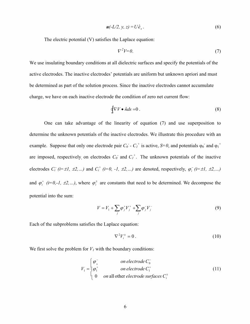
The electric potential (V) satisfies the Laplace equation:

∇ 2V=0. (7)

We use insulating boundary conditions at all dielectric surfaces and specify the potentials of the

active electrodes. The inactive electrodes’ potentials are uniform but unknown apriori and must

be determined as part of the solution process. Since the inactive electrodes cannot accumulate

charge, we have on each inactive electrode the condition of zero net current flow:

0ˆ∫ =•∇s

dsnV . (8)

One can take advantage of the linearity of equation (7) and use superposition to

determine the unknown potentials of the inactive electrodes. We illustrate this procedure with an

example. Suppose that only one electrode pair C0- - C1

+ is active, S=0, and potentials φ0- and φ1

+

are imposed, respectively, on electrodes C0- and C1

+. The unknown potentials of the inactive

electrodes Ci- (i=±1, ±2,…) and Ci

+ (i=0, -1, ±2,…) are denoted, respectively, (i=±1, ±2,…)

and (i=0,-1, ±2,…), where are constants that need to be determined. We decompose the

potential into the sum:

−iϕ

+iϕ ±

iϕ

∑∑ −−++ ++=j

jjj

jj VVVV ϕϕ1 (9)

Each of the subproblems satisfies the Laplace equation:

. (10) 02 =∇ ±iV

We first solve the problem for V1 with the boundary conditions:

(11)

=±

++

−−

iCsurfaceselectrodeonCelectrodeonCelectrodeon

V other all 0

11

0

1

0

ϕϕ

6

Subsequently, we solve the Laplace equations for V (j =0, -1, ±2,…) and V (j =±1, ±2,…)j

+

j

−

with the boundary conditions:

(12)

=±≠

±±

ij

i

C surfaces electrodeother allon 0C electrodeon 1

iV

The unknowns (j=±1, ±2,…) and −jϕ +

jϕ (j=0, -1, ±2,…) are then obtained from the zero net

current flow conditions:

0ˆ =•∇∫js jdsnV . (13)

Alternatively, one can solve for the potential field by implementing equations (13)

directly in the finite element code. This procedure increases the number of variables in the

problem to include the unspecified potentials as unknowns while using equations (13) as

additional equations. When there are many electrodes with unspecified potentials, the

augmented system proved to be more convenient to use. We carried out the calculations of the

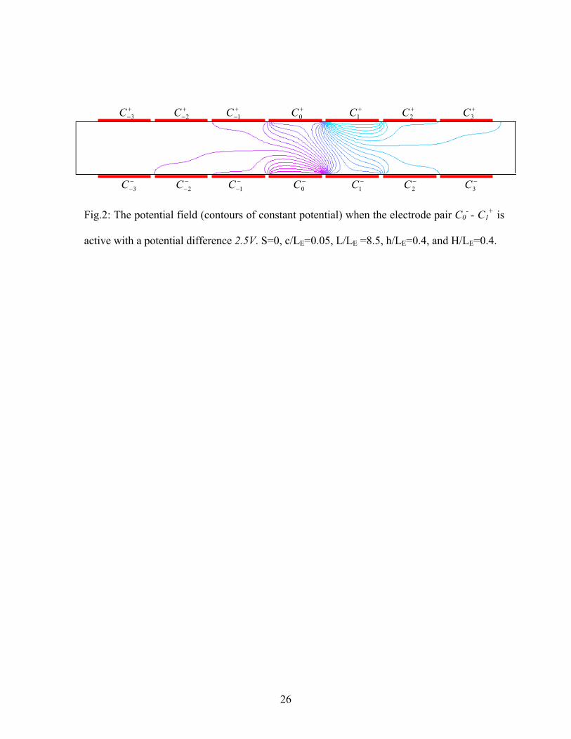
potential field with FEMLAB+. Fig. 2 depicts contours of constant potential lines at the

conduit’s mid-plane (z=H/2) when c/LE=0.05, L/LE=8.5, H/LE=0.4, h/LE=0.4, S=0, /−0ϕ maxϕ =1,

and /+1ϕ maxϕ =0.

Once the potential field was determined, we solved equation (1) for the current density by

dropping the second term since it is much smaller than the first one and then solving equations

(2) and (3) for the velocity field.

Trajectories of passive tracer particles are then obtained by integrating the kinematic

equations,

),( tdtd xux

= , (14)

+ FEMLAB is a product of Comsol Inc., Sweden

7

where x=x,y,z is the position vector.

Fig. 3 depicts trajectories of passive tracer particles injected into the fluid at various

locations at the conduit’s mid-height (z=2H ) in the absence of through flow. The conditions are

the same as in Fig. 2. The flow field was computed with the computational fluid dynamics

software CFD-ACE*. Clearly, the MHD flow is effective in moving material from one side of the

conduit to the other. For example, when half of the conduit is initially filled with species M and

the other half with species N, the interface stretches and deforms to form spiral like tongues with

one material penetrating into the other similar to the pattern depicted in Fig. 10 of [7]. We refer

to the flow pattern depicted in Fig. 3 as flow pattern A and to the corresponding velocity field as

uA. A nearly mirror image of the flow pattern depicted in Fig. 3 forms when one applies the

potential difference across the diagonal electrodes C-1+ and C0

-. We refer to the latter flow pattern

as pattern B and the corresponding velocity field as uB.

When either flow pattern A or B acts alone, it does, indeed, advect material from one side

of the conduit to the other, enhancing mixing. Although much faster than diffusion alone, the

stretching rate of the interface between the two fluids M and N is still relatively slow and scales

approximately like (t+1)ln(t+1) [7]. One can do better, however. By periodically or

aperiodically alternating between flow patterns A and B, one can obtain more complicated

trajectories of the passive tracer particles and achieve chaotic advection which elongates the

length of the interface between M and N at an exponential rate.

Here, we use the temporally periodic protocol:

+<<+=∆=

+<<=∆=

−+−

+−

)1)Tk(t2T(kT .0 and ,

)2TkTtkT ( ,0 and ,

01

10

ϕϕ

ϕϕ

V

V, (15)

* CFD-ACE is a product of CFDRC Inc. USA

8

where k is an integer (k=0,1,…), and T is the period. During the first half period, electrode C-1+

is disconnected, and the electrode pair C0- and C1

+ is active with a potential difference ∆V1. In the

second half period, electrode C1+ is disconnected, and the electrode pair C-1

+ and C0- is active

with a potential difference ∆V2. We will study only the special case of ∆V1=∆V2=∆V. The

protocol described by equation (15) is just one example of numerous possibilities. The choice of

the most effective protocol is an interesting optimization problem that we do not address here.

To visualize the stirrer’s action, we follow the rate of spread of a reagent in the stirring

zone. We denote the dimensionless concentration of the species with G. The concentration is

normalized with its largest value. Let the dark color (Fig. 4) denote the absence of species G

(G(x, t)=0) and the light color indicate the presence of species G at its highest concentration

(G(x,t)=1). Initially (Fig. 4a), the dark color fluid occupies the conduit’s lower section (y<0) and

the light color fluid occupies the conduit’s upper section (y>0).

. (16)

><

=0 ,10 ,0

)0,,,(yy

zyxG

To track the stirring process, we solve the advection equation

GDGtG 2∇=∇⋅+

∂∂ u , (17)

with the boundary conditions 0ˆ =• nG∇ at all solid boundaries and ( ) 0ˆ =•+∇− nGGD u at

x=±L/2, where, typically, L/LE∼8. In the above, D is the molecular diffusion coefficient, and we

assume that the fluid’s properties are not significantly affected by the change in the concentration

of the dissolved species.

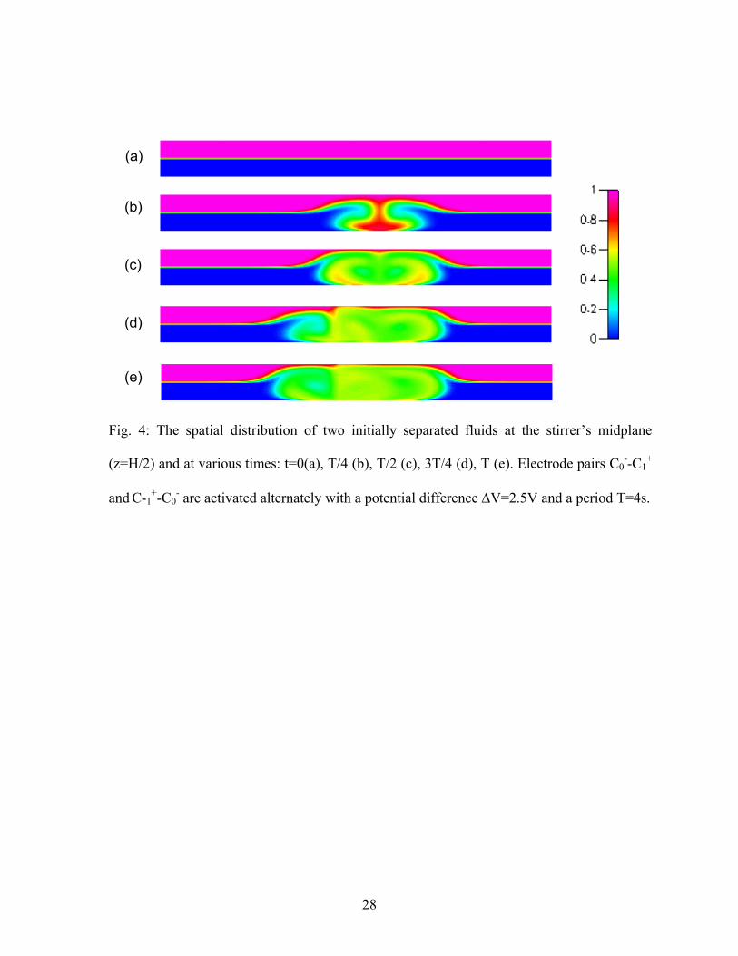
Fig. 4 depicts the concentration G(x,y,H/2,t) as a function of x and y at times t=0 (a), T/4

(b), T/2 (c), 3T/4 (d), and T (e) when the two pairs of electrodes C0--C1

+ and C-1+-C0

- are actuated

alternately with a period T=4s and there is no net flow. The diffusion coefficient D=1.0×10-

11m2/s; the imposed potential difference ∆V=2.5V; the length of an individual electrode is

9

LE=10mm; the gap between adjacent electrodes c=0.5mm; the displacement S=0; and the length,

width, and height of the conduit are, respectively, L=85mm, 2h=8mm, and H=4mm. The figure

illustrates rapid mixing in the stirred region. Within one period, the distinction between the dark

and light has nearly disappeared in the stirring region. Away from the stirring region, the two

fluids remain well separated. The engagement of a larger number of electrodes would increase

the volume of the stirred fluid.

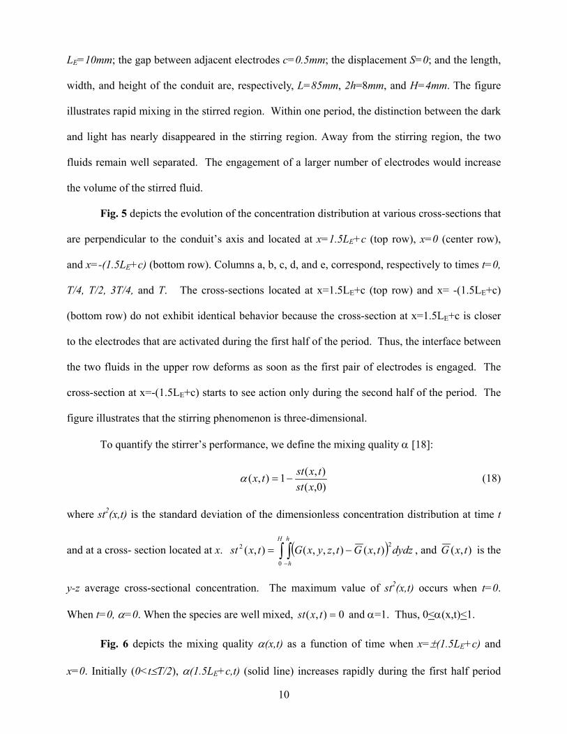
Fig. 5 depicts the evolution of the concentration distribution at various cross-sections that

are perpendicular to the conduit’s axis and located at x=1.5LE+c (top row), x=0 (center row),

and x=-(1.5LE+c) (bottom row). Columns a, b, c, d, and e, correspond, respectively to times t=0,

T/4, T/2, 3T/4, and T. The cross-sections located at x=1.5LE+c (top row) and x= -(1.5LE+c)

(bottom row) do not exhibit identical behavior because the cross-section at x=1.5LE+c is closer

to the electrodes that are activated during the first half of the period. Thus, the interface between

the two fluids in the upper row deforms as soon as the first pair of electrodes is engaged. The

cross-section at x=-(1.5LE+c) starts to see action only during the second half of the period. The

figure illustrates that the stirring phenomenon is three-dimensional.

To quantify the stirrer’s performance, we define the mixing quality α [18]:

)0,(),(1),(

xsttxsttx −=α (18)

where st2(x,t) is the standard deviation of the dimensionless concentration distribution at time t

and at a cross- section located at x. ( dydztxGtzyxGtxstH h

h∫ ∫

−

−=0

22 ),(),,,(),( ) , and ),( txG is the

y-z average cross-sectional concentration. The maximum value of st2(x,t) occurs when t=0.

When t=0, α=0. When the species are well mixed, 0),( =txst and α=1. Thus, 0<α(x,t)<1.

Fig. 6 depicts the mixing quality α(x,t) as a function of time when x=±(1.5LE+c) and

x=0. Initially (0<t≤T/2), α(1.5LE+c,t) (solid line) increases rapidly during the first half period

10

since it is closer to the electrodes C0--C1

+ engaged during this time interval. In the second half

period, the growth rate of α(1.5LE+c, t) decreases, and then increases again in the third half

period. Similar behavior is repeated by α(-1.5LE-c, t) with a delay of T/2. The very low rate of

increase of α(-1.5LE-c, t) during the first half period (0<t<2s) indicates that diffusion alone plays

a minor role in the stirring process. The cross-section located at x=0 is nearly equally affected

by both flow patterns A and B. Therefore, the mixing quality at x=0 (dash-dot line) increases

most rapidly and lacks the plateaus that are visible in the other two curves.

So far, we have described the operation of the stirrer when the only fluid motion in the

conduit was due to the agitation induced by the stirrer. In other words, no through flow was

present. In certain circumstances, it may be desirable to stir the fluids while it is pumped through

the conduit. Such net fluid motion can either be driven by an external pressure, i.e., the fluid is

pumped continuously with a syringe pump, or by a MHD drive located some distance away from

the stirring region. Other researchers have achieved chaotic advection of fluids moving in micro

channels by perturbing the main flow stream with time-periodic pressure perturbations [19] or

exploiting electro-kinetic instabilities under high-voltage AC electric fields [20]. Here, we

perturb the main stream with MHD.

We consider the case of zero electrode displacement (S=0). We connect all the upper,

odd-numbered electrodes Ci+ (i=±1, ±3,…) to form the single electrode “TO;” all the lower,

odd-numbered electrodes Ci- (i=±1, ±3,…) to form the single electrode “BO;” all the upper,

even numbered electrodes Ci+ (i=0, ±2, ±4,…) to form the single electrode “TE;” and all the

lower, even numbered electrodes Ci- (i=0, ±2, ±4,…) to form the single electrode “BE.” When

electrode “TO” is connected to one terminal of a power supply and electrode “BE” is connected

to another terminal of the power supply, the resulting Lorentz forces have both axial and

transverse components, thereby inducing both axial motion and cellular convection. Fig. 7

11

depicts the resulting flow field at the conduit’s midplane (z=H/2) when L=80mm, H=2mm,

h=2mm, LE=5mm, c=0.5mm, and S=0mm. Eleven electrodes are patterned along the top (y=h)

and bottom walls (y=-h). The pressure-driven flow is introduced with a uniform axial velocity

),,,2

( tzyLu − =5mm/s. The distance between the entrance and the leading edge of the first

electrode is 10mm. The external magnetic field B=0.4T. The imposed potential differences

between the electrodes TO and BE and between the electrodes BO and TE are ∆V=2.5V. The

conductivity of the electrolyte is σ=2.56 Ω-1m-1, and the diffusion coefficient D=10-11m2/s. The

arrows and the solid lines depict, respectively, the velocity field and the trajectories of passive

tracer particles. In the absence of temporal alternation of the electrodes’ potentials, Fig. 7

illustrates that as the passive tracer particles advect downstream, they trace an oscillatory path

with very little cross-stream transport. To obtain more complicated motions, we will alternately

activate the electrode pairs TO-BE and BO-TE.

To quantify the stirring process, we supply into the conduit a solution such that

><

=−0,00,1

),,,2

(yy

tzyLG (19)

with the initial condition

. (20)

><

=0,00,1

)0,,,(yy

zyxG

Fig. 8 depicts the concentration ),2

,,( tHyxG at the conduit’s midheight at various times

t=0 (a), T/2 (b), T (c), 3T/2 (d), and 2T (e) when the electrode potentials are alternated with

period T. The simulation conditions are similar to the ones detailed in Fig. 7. Fig. 8a depicts the

situation before the stirring electrodes have been activated. Witness that diffusion plays a

minimal role in the mixing process. The concentration distribution along the length of the

conduit remains similar to the inlet distribution. Once the electrodes have been engaged (t>0),

12

the situation changes rapidly. Figures 8b, c, d, and e illustrate the rapid blending. Fig. 9 depicts

the evolution of the cross-sectional (y-z plane) concentration field at x=40mm (first row) and

x=70mm (the second row) as functions of time t=0, T/2, T, 3T/2, and 2T. Witness that most of

the cross-sectional area assumes a nearly uniform color, indicating that the two species are

reasonably well-mixed.

Fig. 10 depicts the mixing quality α as a function of time at the cross-sectional planes

x=10mm (solid line and symbols ), x=40mm (dashed line and symbols ), and x=70mm (dash-

dotted line and symbols ). The stirrer is activated at t=0. Prior to the stirrer’s activation, the

species were well separated (Fig. 8a) and α(0)=0. As time increases, α initially increases rapidly

until it attains an asymptotic value. The cross section x=10mm is at the front edge of the leading

electrode (the entrance of the mixing region). At this location, little time is available for the

stirring process to have an effect, and α is relatively small. To enable visibility, the curve at

x=10mm was magnified, and the corresponding α scale is given on the RHS vertical axis of the

graph. The magnitudes of α at x=40mm and 70mm are much larger, and the corresponding α

values are given on the LHS of the graph. The graphs in Fig. 10 provide the designer with

guidance about how long the stirrer should be to achieve a desired α value.

The effectiveness of the MHD stirrer depends on the relative magnitudes of the net

through flow and the secondary MHD flow. We define the ratio between the force associated

with the MHD-induced secondary flow per unit length (JBcosθDH2) and the viscous force

associated with the through flow per unit length:

U

JBDK H

µθcos2

= . (21)

In the above, θ is the angle between the diagonal line that connects the centers of the active

pair’s electrodes and the y-axis, J is the current density, B is the intensity of the magnetic field, U

13

is the inlet, average axial velocity, µ is the liquid’s viscosity, and DH is the hydraulic diameter of

the conduit.

Fig. 11 depicts the mixing quality α at x=40mm and t=16s as a function of K. When K is

small (K<<1), through flow effects dominate, the MHD secondary flow has little effect, and α

remains small. When 0.8>K>0.2, α increases nearly linearly as K increases. When K>2,

α achieves an asymptotic value. The figure indicates that to achieve effective stirring, K must be

larger than 1.

In the above examples, only two groups of electrodes were activated. More complicated

flow topologies will form when more than two groups are engaged. The selection of the various

parameters such as the gap distance (c) between adjacent electrodes, the displacement (S), the

electrode length (LE), the number of electrode pairs, the stirring protocol, and the dimensions of

the conduit that provide the most efficient stirring process is an interesting optimization problem

that we do not address here.

α is only one figure of merit for the stirrer’s performance. Another important

consideration is the energy consumption of the stirrer. In the case of the MHD stirrer, the energy

consumption depends on the choice of the electrolyte and electrode materials. In fact, with

appropriate choice of electrodes and electrolytes, the stirrer can form a galvanic cell, be self-

driven, and actually produce electrical energy while performing the stirring (or pumping)

function. A few examples of possible choices of electrodes and electrolytes that would lead to

electric energy production are stainless steel and zinc electrodes operating with a strong oxidizer

such as Fe(NO3)3 or an acid as an electrolyte.

14

3. EXPERIMENTAL SET-UP

To illustrate that similar flows to the ones predicted in the previous section can be

observed in practice, we fabricated two prototypes of MHD stirrers with elastomer

Polydimethylsiloxane (PDMS, Dow Corning Sylgard Elastomer 184, base and a curing agent

with volume ratio 10:1). PDMS has been widely used to form microfluidic components, and it

provides a convenient platform for rapid prototyping [21]. To facilitate easy flow visualization,

the device was made relatively large. Fig.12 depicts schematically the experimental device,

which consists of a Y-shaped micro channel equipped with several electrodes positioned along

the opposing walls.

A copper sheet was glued on a 1.5mm thick, polycarbonate slab. The copper was then

machined with a computer-controlled milling machine (Fadal 88 HS) to form individual

electrodes (with a gap c=0.5mm between two adjacent electrodes) and electrode leads.

Electrodes with lengths of 10mm and 5mm were machined. The former were used in the closed

cavity experiments, and the latter in the flow through experiments.

A polycarbonate template in the shape of the stirrer cavity was milled and positioned on a

glass substrate. The closed stirrer’s template consisted of a rectangular slab

(L×W×H=85mm×8mm×2mm) while the flow-through stirrer’s template was shaped like a Y

(L×W×H=85mm×4mm×2mm). The leading edge of the first electrode was 10mm downstream

from the straight conduit’s entrance (the point where the two legs of the Y connect with the

third). Two plastic tubes (1.75mm O.D. and 1.2mm I.D.) were connected to the two legs of the Y.

A third tube was connected to the chamber’s exit. Finally, a PDMS solution was cast around the

template. After curing the PDMS, the template and frame were removed, leaving behind a cavity

with patterned electrodes along its sidewalls. The cavity was capped with a glass slide.

The electrodes were connected via computer-controlled relay actuators and a D/I card

(PCL-725, Advantech Co., Ltd.) to the terminals of two DC-power supplies (Hewlett Packard,

15

HP 6032A). The relays were wired and programmed to switch "on" and "off" each group of

electrodes. The device was positioned on top of a neodymium (NdFeB, Polymag Inc.),

permanent magnet that provided a nearly uniform intensity magnetic field of B~0.4T. The

magnetic field was measured with the aid of a gauss meter. The conduit was filled with 0.5M

CuSO4 electrolyte solution with a conductivity σ≈2.56Ω-1m-1 [22].

In the absence of through flow, the flow field was visualized by introducing either a

single drop of dye or drops of dye with different colors at various locations in the conduit. In the

presence of through flow, one stream with clear fluid and another stream with dye were

introduced in the two legs of the Y. The flow visualization allowed us to obtain only a qualitative

description of the stirring process. The images of the flow field were captured with both video

and still cameras. The movies provided a much more vivid account of the evolution of the dye

tracers.

4. EXPERIMENTAL OBSERVATIONS

First, we compare the predicted potential field with the potential field that actually

existed in our experiments. To this end, we predicted and measured the potential of one of the

inactive electrodes. Fig.13 depicts the potential difference between the inactivate electrode C-1+

and the ground electrode C1+ as a function of the imposed potential difference ∆V between the

engaged electrodes C0- and C1

+. The solid line and the symbols ( ) represent, respectively, the

theoretically calculated values and experimental measurements. Witness the good agreement

between experiment and theory.

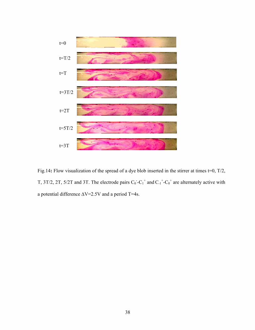
In the absence of through flow, Fig. 14 depicts the flow visualization observations when

electrode pairs C0--C1

+ and C-1

+-C0- were alternately actuated with a period T=4s and potential

difference ∆V=2.5V. Initially, a drop of red dye was introduced into the conduit to

16

approximately occupy the region adjacent to a single electrode pair (t=0). As time increased, so

did the area occupied by the dye. The figure depicts the images of the dye spread at times t=0,

T/2, T, 3T/2, 2T, 5T/2, and 3T. The figure illustrates the rapid stirring processes. The images are

consistent with chaotic stirring. When t=3T=12s, the dye has occupied the entire stirring region

(length of 3 electrodes). Throughout the experiment, we monitored carefully for bubble

formation. No bubble production was observed.

The spread of the dye is facilitated by both diffusion and advection. To verify that

diffusion alone did not play a significant role in our experiments, we introduced a drop of dye

into the conduit and followed its spread without activating the stirrer. During the time interval of

a typical experiment (about 40s), only a very small spread of the dye was observed. Diffusion did

not appear to play a significant role in our experiments.

The stirring process is described more vividly in Fig. 15. Red and green dye blobs were

introduced into the conduit, and their evolution was tracked as a function of time. At t=0, the red

and the green dyes were well separated (Fig.15, t=0). After one period, some of the red dye was

surrounded by the green dye (Fig. 15, t=T). As time increased, through continuous stretching and

folding which are characteristic of chaotic advection, the two dyes blended.

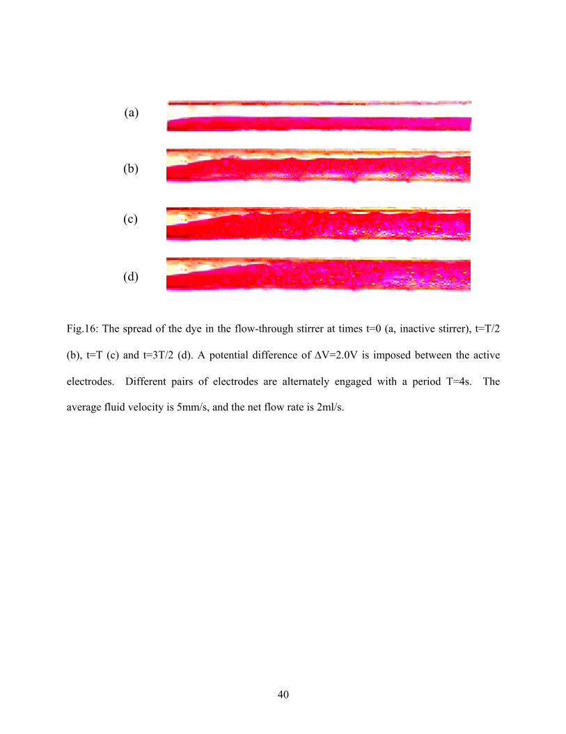
For continuous, through-flow mixing, the two inlet legs of the Y-shaped conduit were

connected to two computer-controlled syringe pumps (KDScientific Inc., model 200 series). We

first filled the channel with DI water and then injected dye through one leg of the Y and clear

electrolyte solution through the other leg. The total inlet flow rate was 2ml/s. When the mixer

was not activated, the two streams were separate. One side of the conduit (y<0) was occupied

with the dye while the other side (y>0) was occupied with the colorless electrolyte (Fig. 16a).

The two fluids flowed downstream side by side with very little mixing. When the mixer was

activated by alternating the electrode pairs TO-BE and BO-TE, the Lorenz force drove secondary

flows, and the two streams mixed rapidly. Figs. 16b, c, and d depict the spread of the dye at

17

times t=T/2, T and 3T/2 when T=4s. The experimental observations (Fig.16) are in qualitative

agreement with the theoretical predictions (Fig. 8).

5. DISCUSSION AND CONCLUSIONS

The paper describes a magneto-hydrodynamic stirrer that does not require any interior

electrodes. The stirrer consists of a conduit filled with an electrolyte solution and positioned in a

magnetic field. Individually controlled electrodes are positioned along the conduit’s opposing

sidewalls. By appropriate adjustment of the potential differences across the wall-electrodes, one

can use the resulting Lorentz forces to either pump or stir the fluid. When a potential difference

is applied across opposing electrodes, the device operates as a pump. When the potential

difference is applied across two or more diagonally positioned electrodes, secondary flows are

induced. By alternating between different flow patterns, one can induce chaotic advection.

Moreover, the stirrer can also operate with continuous, through flows. We demonstrated in both

experiment and theory that it is possible to induce efficient stirring with this type of a MHD

stirrer. Since there are no moving mechanical parts, similar (scaled down) stirrer designs are

appropriate for various microfluidic applications. When reducing the device’s size, one must

keep in mind, however, that the Lorentz forces are volumetric in nature and decline rapidly in

magnitude as the stirrer’s volume decreases.

The MHD pump and stirrer described here are not completely problem-free. Some

potential problems are bubble formation, electrode corrosion, and migration of analytes in the

electric field. Most of these problems can, however, be reduced or eliminated altogether with

appropriate selection of electrolytes, electrode materials and operating conditions. Bubble

formation is not likely to be a problem at sufficiently low potential differences (smaller than the

potential needed for the electrolysis of water). Electrode corrosion may be tolerated in disposable

18

devices or minimized with the use of passivated electrodes. RedOx solutions such as FeCl2 /

FeCl3, potassium ferrocyanide trihydrate (K4[Fe(CN)6]×3H2O) / potassium ferricyanide

(K3[Fe(CN)6]), and hydroquinone in combination with inert electrodes provide relatively high

current densities at low electrodes’ potential differences without any electrode corrosion, bubble

formation, and electrolyte depletion.

ACKNOWLEDGMENTS

Drs. Z. Chen, S-C Kweon, and J. Wang (University of Pennsylvania) assisted with the

construction of the experiment. The work was supported, in part, by DARPA'S SIMBIOSYS

PROGRAM (Dr. Anantha Krishnan, program director) through grant N66001-01-C-8056 to the

University of Pennsylvania.

19

REFERENCES

[1] H. H. Woodson and J.R. Melcher, Electromechanical Dynamics, Vol. III, John Wiley, 1969

[2] P. A. Davidson, An Introduction to Magnetohydrodynamics, Cambridge Press, 2001

[3] J. Jang, S.S. Lee, Theoretical and Experimental Study of MHD (Magnetohydrodynamic)

Micropump, Sensors and Actuators A, 80(2000), 84-89.

[4] A.V. Lemoff, A.P. Lee, An AC Magnetohydrodynamic Micropump, Sensors and Actuators

B, 63 (2000), 178-185.

[5] H.H. Bau, A Case for Magneto-hydrodynamics (MHD), IMECE 2001, MEMS 23884

Symposium Proceedings, N.Y., Nov 2001

[6] J. Zhong, M. Yi, H.H. Bau, Magneto-hydrodynamic (MHD) Pump Fabricated with Ceramic

Tapes, Sensors and Actuators A, 96 (2002), 59-66

[7] H.H. Bau, J. Zhong, and M. Yi, A Minute Magneto Hydro Dynamic (MHD) Mixer, Sensors

and Actuators B, 79 (2001), 205-213.

[8] H.H. Bau, J. Zhu, S. Qian, Y. Xiang, A Magneto-Hydrodynamic Micro Fluidic Network,

IMECE 2002-33559, Proceedings of IMECE'02, 2002 ASME International Mechanical

Engineering Congress & Exposition, New Orleans, Louisiana, November 17-22, 2002

[9] H.H. Bau, J. Zhu, S. Qian, Y. Xiang, A Magneto-hydrodynamically Controlled Fluidic

Network, Sensors and Actuators B, 88 (2003), 207-218

[10] J. West, B. Karamata, B. Lillis, J.P. Gleeson, J. Alderman, J.K. Collins, W. Lane, A.

Mathewson, H. Berney, Application of Magnetohydrodynamic Actuation to Continuous

Flow Chemistry, Lab on a Chip, 2 (2002), 224-230

[11] J. Gleeson and J. West, Magnetohydrodynamic Micromixing, Technical Proceedings of the

Fifth International Conference on Modeling and Simulation of Microsystems, Puerto Rico,

318-321, 2002

20

[12] G. Taylor, Dispersion of Soluble Matter in Solvent Flowing Slowly through a Tube,

Proceedings of the Royal Society of London Series A-Mathematical and Physical Sciences,

219 (1953),186-203.

[13] H. Aref, Stirring by Chaotic Advection, J. Fluid Mechanics, 143(1984), 1-21.

[14] M. Yi, S. Qian, H.H. Bau, A Magnetohydrodynamic Chaotic Stirrer, Journal of Fluid

Mechanics, 468 (2002), 153-177

[15] S. Qian, J. Zhu , H.H. Bau, A Stirrer for Magnetohydrodynamically Controlled Minute

Fluidic Networks, Physics of Fluids, 14 (2002), 3584-3592

[16] S. Qian, H.H. Bau, A Chaotic Electroosmotic Stirrer, Analytical Chemistry, 74 (2002),

3616-3625

[17] Y. Xiang, H.H. Bau, Complex Magnetohydrodynamic Low-Reynolds-Number Flows,

Physical Review E, 68 (2003), 016312

[18] N. Kockmann, C. Föll, P. Woias, Flow Regimes and Mass Transfer Characteristics in Static

Micro Mixers, SPIE 8982-38, Photonics West, Micromachining and Microfabrication, San

Jose, January 27-29,2003.

[19] Y. K. Lee, J. Deval, P. Tabeling, and C.M. Ho, Chaotic Mixing in Electrokinetically and

Pressure Driven Micro Flows, Proc. 14th IEEE workshop on Micro Electro Mechanical

Systems (Interlaken, Switzerland) January 2001, 483-486

[20] M. H. Oddy, J. G. Santiago, and J. C. Mikkelsen, Electrokinetic Instability Micromixing,

Analytical Chemistry, 73(2002), 5822-5832

[21] E. Delamarche, H. Schmid, B. Michel, and H. Biebuyck, Stability of Molded

Polydimethylsiloxane Microstructures, Advanced Materials, 9 (1997), 741-746

[22] J.A. Dean, Lange's Handbook of Chemistry, the 15th edition, New York: McGraw-Hill,

1999

21

LIST OF CAPTIONS

1. A schematic, top view of the stirrer’s cavity. The cavity is equipped with numerous

individual electrodes, (Ci+) and (Ci

-), positioned along opposite walls. The length of each

electrode is LE, the gap between adjacent electrodes is c, and the electrodes are staggered

with shift S.

2. The potential field (contours of constant potential) when the electrode pair C0- - C1

+ is

active with a potential difference 2.5V. S=0, c/LE=0.05, L/LE =8.5, h/LE=0.4, and

H/LE=0.4.

3. The simulated flow field in the vicinity of the active electrode pair C0- - C1

+. The figure

depicts the trajectories of passive tracer particles at the conduit’s mid-height. The

potential difference ∆V=2.5V, S=0, c/LE=0.05, L/LE =8.5, h/LE=0.4, H/LE=0.4, B=0.4T,

and σ=2.56 Ω-1m-1.

4. The spatial distribution of two initially separated fluids at the stirrer’s midplane (z=H/2)

and at various times: t=0(a), T/4 (b), T/2 (c), 3T/4 (d), T (e). Electrode pairs C0--C1

+ and

C-1+-C0

- are activated alternately with a potential difference ∆V=2.5V and a period T=4s.

5. The spatial distribution of two initially separated fluids at cross-sections x= (1.5LE+c) (I),

x=0(II), and x=-(1.5LE+c) (III) and times t=0 (a), T/4 (b), T/2 (c), 3T/4 (d), and T(e).

Electrode pairs C0--C1

+ and C-1+-C0

- are activated alternately with a potential difference

∆V=2.5V and a period T=4s.

6. The mixing quality (α) as a function of time at cross-sections x=1.5LE+c (solid line), x=0

(dash-dot line), and x=-(1.5LE+c) (dashed line). Electrode pairs C0--C1

+ and C-1+-C0

- are

alternately active with a potential difference ∆V=2.5V and a period T=4s.

22

7. The flow field and streak lines in the midplane (z=H/2) when electrode pair TO-BE is

active with a potential difference ∆V=2.5V. The fluid flows continuously through the

straight conduit with average axial velocity U=5mm/s. B=0.4T and σ=2.56 Ω-1m-1.

8. The spatial distribution of two initially separated fluids at the midplane (z=H/2) at times

t=0 (a), T/2(b), T(c), 3T/2(d), and 2T (e). The fluids flow continuously through the

straight conduit with average axial velocity U=5mm/s. The electrode pairs TO-BE and

BO-TE are alternately active with an imposed potential difference ∆V=2.5V and a period

T=4s. B=0.4T, D=10-11 m2/s and σ=2.56 Ω-1m-1.

9. The spatial distribution of two initially separated fluids at cross-sections x=40mm (I) and

x=70mm (II) and at times t=0 (a), t=T/2(b), t=T(c), t=3T/2 (d), and t=2T (e). The fluids

flow continuously through the straight conduit with an average axial velocity U=5mm/s.

The electrode pairs TO-BE and BO-TE are alternately active with an imposed potential

difference ∆V=2.5V and a period T=4s. B=0.4T, D=10-11 m2/s and σ=2.56 Ω-1m-1.

10. The mixing quality α in the flow-through reactor as a function of time at cross-sections

x=10mm (solid line and symbols ), x=40mm (dashed line and symbols ), and

x=70mm (dash-dot line and symbols ). The fluids flow continuously through the

straight conduit with an average axial velocity U=5mm/s. The electrode pairs TO-BE and

BO-TE are alternately active with an imposed potential difference ∆V=2.5V and a period

T=4s. B=0.4T, D=10-11 m2/s, and σ=2.56 Ω-1m-1.

11. The mixing quality α in the flow-through reactor as a function of K at x=40mm, t=4T,

and T=4s.

12. A schematic description of the MHD stirrer (an exploded view).

13. The potential difference ∆V-1 between the inactive electrode C-1+ and the ground

electrode C1+ as a function of the imposed potential difference ∆V0 between the active

23

electrodes C0- - C1

+. The solid line and the symbols (•) represent, respectively, the

theoretical predictions and the measured values.

14. Flow visualization of the spread of a dye blob inserted in the stirrer at times t=0, T/2, T,

3T/2, 2T, 5/2T and 3T. The electrode pairs C0--C1

+ and C-1+-C0

+ are alternately active

with a potential difference ∆V=2.5V and a period T=4s.

15. Images of the blending process when initially well-separated red and green dye blobs are

introduced into the stirrer. The various images correspond to times t=0, T, 2T, 3, 4T, 5T,

6T, and 7T. The electrode pairs C0--C1

+ and C-1+-C0

+ are alternately active with a potential

difference ∆V=2.5V and a period T=4s.

16. The spread of the dye in the flow-through stirrer at times t=0 (a, inactive stirrer), t=T/2

(b), t=T (c) and t=3T/2 (d). A potential difference of ∆V=2.0V is imposed between the

active electrodes. Different pairs of electrodes are alternately engaged with a period

T=4s. The average fluid velocity is 5mm/s, and the net flow rate is 2ml/s.

24

xc

C0-C-3

- C-2- C-1

- C3-C2

- C1-

C0+C-3

+ C-2+ C-1

+ C3+C2

+ C1+

y

2h

S

LE

Fig.1: A schematic, top view of the stirrer’s cavity. The cavity is equipped with numerous

individual electrodes, (Ci+) and (Ci

-), positioned along opposite walls. The length of each

electrode is LE, the gap between adjacent electrodes is c, and the electrodes are staggered with

shift S.

25

3210123−−−−−

−−−

−− CCCCCCC

3210123+++++

−+−

+− CCCCCCC

Fig.2: The potential field (contours of constant potential) when the electrode pair C0- - C1

+ is

active with a potential difference 2.5V. S=0, c/LE=0.05, L/LE =8.5, h/LE=0.4, and H/LE=0.4.

26

−0C −

1C −2C−

−1C

+−1C +

1C+0C +

2C

Fig.3: The simulated flow field in the vicinity of the active electrode pair C0- - C1

+. The

figure depicts the trajectories of passive tracer particles at the conduit’s mid-height. The

potential difference ∆V=2.5V, S=0, c/LE=0.05, L/LE =8.5, h/LE=0.4, H/LE=0.4, B=0.4T, and

σ=2.56 Ω-1m-1.

27

(a)

(b)

(c)

(d)

(e)

Fig. 4: The spatial distribution of two initially separated fluids at the stirrer’s midplane

(z=H/2) and at various times: t=0(a), T/4 (b), T/2 (c), 3T/4 (d), T (e). Electrode pairs C0--C1

+

and C-1+-C0

- are activated alternately with a potential difference ∆V=2.5V and a period T=4s.

28

(a) (b) (c) (d) (e)

(I)

(II)

(III) y

z

Fig.5: The spatial distribution of two initially separated fluids at cross-sections x= (1.5LE+c)

(I), x=0(II), and x=-(1.5LE+c) (III) and times t=0 (a), T/4 (b), T/2 (c), 3T/4 (d), and T(e).

Electrode pairs C0--C1

+ and C-1+-C0

- are activated alternately with a potential difference

∆V=2.5V and a period T=4s.

29

Fig.6: The mixing quality (α) as a function of time at cross-sections x=1.5LE+c (solid line),

x=0 (dash-dot line), and x=-(1.5LE+c) (dashed line). Electrode pairs C0--C1

+ and C-1+-C0

- are

alternately active with a potential difference ∆V=2.5V and a period T=4s.

30

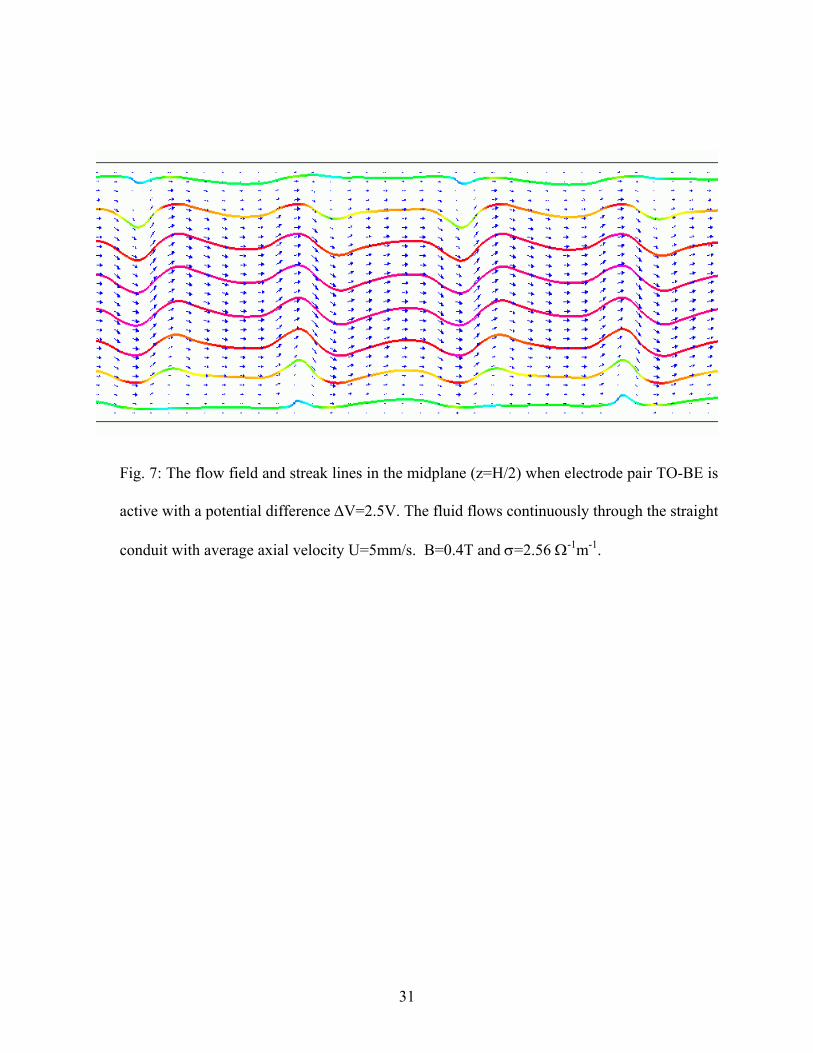
Fig. 7: The flow field and streak lines in the midplane (z=H/2) when electrode pair TO-BE is

active with a potential difference ∆V=2.5V. The fluid flows continuously through the straight

conduit with average axial velocity U=5mm/s. B=0.4T and σ=2.56 Ω-1m-1.

31

(a) (b)

(c) (d) (e)

Fig.8: The spatial distribution of two initially separated fluids at the midplane (z=H/2) at

times t=0 (a), T/2(b), T(c), 3T/2(d), and 2T (e). The fluids flow continuously through the

straight conduit with average axial velocity U=5mm/s. The electrode pairs TO-BE and BO-

TE are alternately active with an imposed potential difference ∆V=2.5V and a period T=4s.

B=0.4T, D=10-11 m2/s and σ=2.56 Ω-1m-1.

32

(a) (b) (c) (d) (e)

(II)

(I)

y

z

Fig.9: The spatial distribution of two initially separated fluids at cross-sections x=40mm (I)

and x=70mm (II) and at times t=0 (a), t=T/2(b), t=T(c), t=3T/2 (d), and t=2T (e). The fluids

flow continuously through the straight conduit with an average axial velocity U=5mm/s. The

electrode pairs TO-BE and BO-TE are alternately active with an imposed potential difference

∆V=2.5V and a period T=4s. B=0.4T, D=10-11 m2/s and σ=2.56 Ω-1m-1.

33

Fig.10: The mixing quality α in the flow-through reactor as a function of time at cross-

sections x=10mm (solid line and symbols ), x=40mm (dashed line and symbols ), and

x=70mm (dash-dot line and symbols ). The fluids flow continuously through the straight

conduit with an average axial velocity U=5mm/s. The electrode pairs TO-BE and BO-TE are

alternately active with an imposed potential difference ∆V=2.5V and a period T=4s. B=0.4T,

D=10-11 m2/s, and σ=2.56 Ω-1m-1.

34

Fig.11: The mixing quality α in the flow-through reactor as a function of K at x=40mm,

t=4T, and T=4s.

35

Flow conduits

connectors

electrodes

cap

Fig.12: A schematic description of the MHD stirrer.

36

∆V-1(v)

∆V0(v)

Fig.13: The potential difference ∆V-1 between the inactive electrode C-1+ and the ground

electrode C1+ as a function of the imposed potential difference ∆V0 between the active electrodes

C0- - C1

+. The solid line and the symbols (•) represent, respectively, the theoretical predictions

and the measured values.

37

t=0

t=T/2

t=T

t=3T/2

t=2T

t=5T/2

t=3T

Fig.14: Flow visualization of the spread of a dye blob inserted in the stirrer at times t=0, T/2,

T, 3T/2, 2T, 5/2T and 3T. The electrode pairs C0--C1

+ and C-1+-C0

+ are alternately active with

a potential difference ∆V=2.5V and a period T=4s.

38

t=0

t=T

t=2T

t=3T

t=4T

t=5T

t=6T

t=7T

Fig. 15: Images of the blending process when initially well-separated red and green dye

blobs are introduced into the stirrer. The various images correspond to times t=0, T, 2T, 3,

4T, 5T, 6T, and 7T. The electrode pairs C0--C1

+ and C-1+-C0

+ are alternately active with a

potential difference ∆V=2.5V and a period T=4s.

39

40

(a)

(b)

(c)

(d)

Fig.16: The spread of the dye in the flow-through stirrer at times t=0 (a, inactive stirrer), t=T/2

(b), t=T (c) and t=3T/2 (d). A potential difference of ∆V=2.0V is imposed between the active

electrodes. Different pairs of electrodes are alternately engaged with a period T=4s. The

average fluid velocity is 5mm/s, and the net flow rate is 2ml/s.