Forecasting Non-Stationary Diarrhea, Acute Respiratory ...

Forecasting Non-Stationary Diarrhea, Acute RespiratoryInfection, and Malaria Time-Series in Niono, MaliDaniel C. Medina1,3, Sally E. Findley2*, Boubacar Guindo3, Seydou Doumbia3

1 College of Physicians and Surgeons, Columbia University, New York, New York, United States of America, 2 Department of Population and FamilyHealth, Mailman School of Public Health, Columbia University, New York, New York, United States of America, 3 Malaria Research and Training Center,Faculte de Medecine de Pharmacie et d’Odonto-Stomatologie (FMPOS), Universite de Bamako, Bamako, Mali

Background. Much of the developing world, particularly sub-Saharan Africa, exhibits high levels of morbidity and mortalityassociated with diarrhea, acute respiratory infection, and malaria. With the increasing awareness that the aforementionedinfectious diseases impose an enormous burden on developing countries, public health programs therein could benefit fromparsimonious general-purpose forecasting methods to enhance infectious disease intervention. Unfortunately, these diseasetime-series often i) suffer from non-stationarity; ii) exhibit large inter-annual plus seasonal fluctuations; and, iii) requiredisease-specific tailoring of forecasting methods. Methodology/Principal Findings. In this longitudinal retrospective (01/1996–06/2004) investigation, diarrhea, acute respiratory infection of the lower tract, and malaria consultation time-series arefitted with a general-purpose econometric method, namely the multiplicative Holt-Winters, to produce contemporaneous on-line forecasts for the district of Niono, Mali. This method accommodates seasonal, as well as inter-annual, fluctuations andproduces reasonably accurate median 2- and 3-month horizon forecasts for these non-stationary time-series, i.e., 92% of the 24time-series forecasts generated (2 forecast horizons, 3 diseases, and 4 age categories = 24 time-series forecasts) have meanabsolute percentage errors circa 25%. Conclusions/Significance. The multiplicative Holt-Winters forecasting method: i)performs well across diseases with dramatically distinct transmission modes and hence it is a strong general-purposeforecasting method candidate for non-stationary epidemiological time-series; ii) obliquely captures prior non-linearinteractions between climate and the aforementioned disease dynamics thus, obviating the need for more complexdisease-specific climate-based parametric forecasting methods in the district of Niono; furthermore, iii) readily decomposestime-series into seasonal components thereby potentially assisting with programming of public health interventions, as well asmonitoring of disease dynamics modification. Therefore, these forecasts could improve infectious diseases management in thedistrict of Niono, Mali, and elsewhere in the Sahel.

Citation: Medina DC, Findley SE, Guindo B, Doumbia S (2007) Forecasting Non-Stationary Diarrhea, Acute Respiratory Infection, and Malaria Time-Series in Niono, Mali. PLoS ONE 2(11): e1181. doi:10.1371/journal.pone.0001181

INTRODUCTIONTemperature and pluviometric fluctuations affect water resources,

food production, and disease transmission [1–5]. In Africa, these

fluctuations are coupled to i) the El Nino southern oscillator

(ENSO), which impacts eastern and southern Africa the most; as

well as, ii) the Atlantic dipole (AD) and the inter-tropical

convergence zone (ITCZ) [6], which intimately govern climate

thus potentially imparting famine and exacerbating disease

transmission in the Sahel (Figure 1)—i.e., the sub-Saharan

region that spans the entire east-west African axis, bordering the

Sahara desert to the north and the Savanna to the south.

In much of the Sahel, climate-coupled diarrhea, acute re-

spiratory infection of the lower tract (ARI), and malaria

transmission continue to inflict most morbidity and mortality.

Diarrhea transmission heightens during the rainy season pre-

sumably because of facilitated fecal contamination of water sources

[7–10]. Diarrhea has multiple etiologies in the district of Niono.

Viral diarrhea (e.g., Rotavirus sp.) is typical among infants; bacterial

(e.g., S. enterica) and protozoan (e.g., E. histolytica) infection are more

commonly diagnosed among older individuals. ARI incidence

often culminates biannually during the dry season and again

towards the end of the rainy season [1,11–16]. ARI also has

multiple etiologies in the district of Niono. Viral ARI (e.g., Human

respiratory syncytial virus) is common among infants whereas, e.g., H.

influenza and S. pneumoniae infection are more frequently diagnosed

in older age categories. Last, malaria transmission behaves

seasonally (or perennially) with a periodic intensification that

follows the rainy season onset. P. falciparum, which is transmitted by

the Anopheles s.p. vector, is the predominant pathogen (.99%)

underlying malaria infection in Mali. Like diarrhea and ARI, the

diagnosis of malaria is usually clinical in the district of Niono and

much of the Sahel. Malaria affects those who have greater

susceptibility to infection: i) children under 5 years of age who

have not yet developed low-level immunity; ii) mal-nourished

pregnant women; and iii) labor migrants from non-endemic zones

who, like children under 5 years of age, lack low-level immunity

[17–22]. Furthermore, pervasive malnutrition—which precedes

harvesting and partially coincides with diarrhea, ARI, and malaria

transmission zeniths—aggravates (and probably underlies) the

somber epidemiological scenario crafted by the aforementioned

diseases in the Sahel [7,23,24].

With the increasing awareness that infectious diseases impose an

enormous burden on developing countries, public health programs

Academic Editor: Colin Sutherland, London School of Hygiene & TropicalMedicine, United Kingdom

Received May 8, 2007; Accepted October 18, 2007; Published November 21, 2007

Copyright: � 2007 Medina et al. This is an open-access article distributed underthe terms of the Creative Commons Attribution License, which permitsunrestricted use, distribution, and reproduction in any medium, provided theoriginal author and source are credited.

Funding: The Climate and Society Program (Earth Institute, Columbia University,New York, NY, USA) partially funded data collection and analyses.

Competing Interests: The authors have declared that no competing interestsexist.

* To whom correspondence should be addressed. E-mail: [email protected]

PLoS ONE | www.plosone.org 1 November 2007 | Issue 11 | e1181

therein could benefit from parsimonious general-purpose quanti-

tative methods to enhance local intervention, i.e., diminish

infectious disease-induced morbidity and mortality. Quantitative

methods are particularly important for Sahelian countries—which

rank among the poorest in the world—where the deployment of

scarce resources is tantamount to a budgetary sacrifice. Conse-

quently, disease risk assessment [25–30], epidemiologic forecasts

[31–35], and early warning systems [36] are de rigueur before

interventions can effectively mitigate the morbidity and mortality

that infectious diseases inflict. In the context of forecasts,

epidemiological time-series (TS) often i) exhibit inter-annual plus

seasonal fluctuations; ii) require disease-specific tailoring of fore-

casting methods; and, iii) suffer from non-stationarity. [Stationary

time-series (e.g., white-noise) have time-independent mean and

covariance structures; conversely, non-stationary time-series (e.g.,

inventory) have time-dependent mean and covariance structures.]

Therefore, a general-purpose econometric method, namely the

(seasonal) multiplicative Holt-Winters (MWH) [37,38], is em-

ployed herein to forecast epidemiologically distinct non-stationary

diarrhea, ARI, and malaria consultation rate TS for the district of

Niono [39,40], Mali (Fig. 1). The MHW method is extensively

described in the Methods section and schematically depicted in

Figure 2. This method ignores direct effects from climate (e.g.,

AD and ITCZ) on disease TS. Nevertheless, MHW-based

historical TS analyses can obliquely capture non-linear prior

interactions between climate and the aforementioned disease

dynamics thus, potentially obviating the need for more complex

disease-specific climate-based parametric forecasting methods

(which are otherwise indispensable for highly-unstable trans-

mission and or spatially-extended infectious disease models) in the

district of Niono. This method could directly improve infectious

disease management in this district with potential repercussions

elsewhere in the Sahel where quantitative approaches may assist

with predicting and containing infectious disease-induced mor-

bidity and mortality.

RESULTS

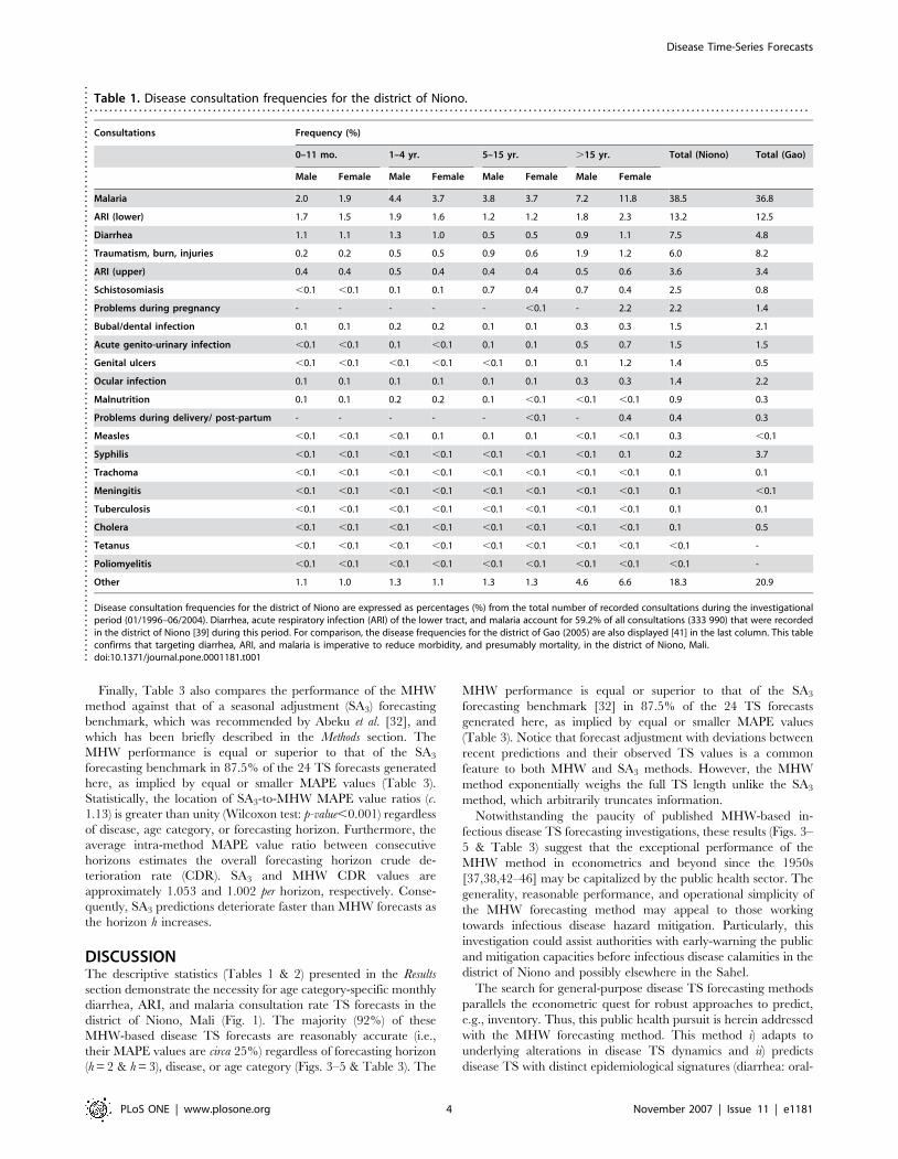
Consultation frequenciesAltogether, diarrhea, ARI, and malaria account for 59.2% of all

consultations (333 990) during the investigational period (01/

1996–06/2004) in the district of Niono [39], each perpetrating

7.5%, 13.2%, and 38.5% of total recorded morbidity, respectively

(Table 1). A larger proportion of male than female individuals

under 16 years of age are diagnosed with the aforementioned

diseases; the converse is true for adults presumably because of

differential risk-factor exposure. For comparison, Table 1 also

displays the disease frequency distribution, based upon records

from a single semester, for the district of Gao (last column) at

approximately the same latitude but further east [41]. Though

further investigations are necessary, the striking resemblance

between these two record distributions further suggests epidemi-

ological similarities across the Sahel. Consultation frequency

distributions for the districts of Niono and Gao (Table 1) indicate

that targeting diarrhea, ARI, and malaria is imperative to reduce

morbidity (presumably mortality) in the district of Niono and

possibly elsewhere in the Sahel. Of note, the reported malnutrition

consultation frequency (0.9%) seems unrealistic when compared to

the prevalence of stunted, under-weight, and wasted individuals in

Mali, i.e., approximately 38%, 33%, and 11%, respectively [40].

Diarrhea, ARI, and malaria consultation ratesAge category-specific median annual diarrhea, ARI, and malaria

consultation rates, as well as corresponding inter-quartile range

(IQR) values, for each of the 17 community health center

(CSCOM) service areas within the district of Niono are reported in

Table 2. Median annual consultation rates are expressed as the

number of newly diagnosed cases per 1000 individuals in an age

category during a year. Median annual consultation rates for

younger age categories (Table 2) are disproportionately greater

than their consultation frequencies (Table 1) because of age

composition [40]. Generally, these rates diminish towards older

age categories; hence, the systematic consultation rate age-

dependence across CSCOM service areas emphasizes the need

for age category-specific forecasts.

A non-parametric ‘analog’ of the coefficient of variance, i.e., the

ratio of IQR-to-median values, robustly measures annual

consultation rate dispersion for each CSCOM service area.

Notwithstanding the large median annual consultation rate

variability across CSCOM service areas, CSCOM-specific ratios

of IQR-to-median values are also large (not shown). Consequently,

spatially-temporal forecasts for the district of Niono seem

unnecessary in this initial developmental phase.

Figure 1. Map of West Africa. Panel A: The Sahara desert and the savannah occupy the northern and southern landscape, respectively, while theSahel comprises the intermediate fringe zone. Mali lacks access to the ocean; its capital, Bamako, is indicated with a red pointer; and, the district ofNiono is located inside the red demarcation, which is enlarged in panel B. Panel B: The black line on the top of this panel corresponds to thesoutheastern Mauritanian border; the depicted segment of the Niger River runs along the southwest-northeast direction; the district of Niono, whichis located 330 km northwest of Bamako and 100 km north of the Niger River along the Canal du Sahel, is located within the red rectangle. Thissatellite image places the district of Niono in the Sahelian zone: poverty is extensive in the northern (semi-desert) and central (irrigated) regions;contrarily, poverty diminishes southward (savannah) where mixed crops prevail. Image source: adapted with permission from Globalis, http://globalis.gvu.unu.edu (08/2007).doi:10.1371/journal.pone.0001181.g001

Disease Time-Series Forecasts


Time-series forecastsThe MHW forecasting method has been described in the Methods

section and schematically depicted in Fig. 2. MHW Equation 1

produces point forecasts, which are recursively revised with

Equations 2–4, whilst their 95% prediction interval bounds (PI)

are estimated with Equation 5. Eqs. 1–5 also decompose TS into

level, trend (rate of change), seasonal, and approximately serially

uncorrelated residual TS components, i.e., {lt}, {rt}, {sm|t}, and

{zt}, respectively. MHW pseudo-parameters a, b, and c (Eqs. 2–4)

control exponential smoothing of corresponding lt, rt, and sm|t TS

components. In Figures 3–5, observed age category-specific

amalgamated consultation rate TS for diarrhea (Fig. 3), ARI

(Fig. 4), and malaria (Fig. 5) are symbolized by black lines while

red and blue traces correspond to contemporaneous on-line (fig. 2)

median 2- and 3-month horizon (h) MHW forecasts, respectively;

their 95% PI values are depicted in dots of the same colors.

Abscissa TS projections span 102 months (01/1996–06/2004)

while ordinate values represent the number of newly diagnosed

cases per 1000 age category-specific individuals. TS ordinate scales

diminish with increasing age across panels A (0–11 months), B (1–

4 years), C (5–15 years), and D (.15 years), reflecting the age-

dependent consultation rate distribution elucidated in Table 2.

Malaria (Fig. 5) and diarrhea (Fig. 3) consultations exhibit the

largest and smallest inter-annual fluctuations, respectively, as

intuited from their consultation rate TS (black lines) and implied

by their decomposed {lt} plus {rt} TS components (not shown).

Consultation rate TS evolution (black lines) also reveals dominant

seasonal oscillations in the transmission of diarrhea, ARI, and

malaria (Figs. 3–5). The strength of MHW pseudo-parameters

mostly follow c&a$b, which obtain for highly seasonal TS with

negligible rt components (Table 3). Disease- and age category-

specific 2- and 3-month horizon forecasts roughly overlap because

decomposed {lt} shifts slowly and {rt} approaches nil. Conse-

quently, 2- and 3-month horizon 95% PI values also overlap.

Generally, TS forecasts (Figs. 3–5) are accurate and precise,

varying degrees of seasonal and inter-annual TS fluctuations

notwithstanding.

Forecasts for ARI (Fig. 4) and malaria (Fig. 5) tend to perform

better than those for diarrhea (Fig. 3) consultation rate TS

(Table 3). Forecasts for ARI (Fig. 4) and malaria (Fig. 5)

consultation rate TS deteriorate and ameliorate (though only

faintly), respectively, towards older age categories. Furthermore,

forecasts for diarrhea consultation rate TS (Fig. 3) are reasonably

accurate for panels A (0–11 months), B (1–4 years), and D

(.15 years) where seasonality dominates. Beyond visual inspection

of Figs. 3–5, forecasting accuracy is assessed with mean absolute

percentage error (MAPE) values between observed monthly

consultation rates and their median forecasts (Table 3). These

revolve circa 25% regardless of disease, age category, or forecasting

horizon. The exceptions are: i) the low forecasting accuracy for the

diarrhea consultation rate TS that appears in panel C (5–15 yr.) of

Fig. 3, i.e., 42.4% and 43.5% for h = 2 and h = 3, respectively; and,

ii) the high forecasting accuracy for the malaria consultation rate

TS that appears in panel D (.15 yr.) of Fig. 5, i.e., 17.8% and

18.1% for h = 2 and h = 3, respectively. Notice that 92% of the 24

TS forecasts generated (2 forecast horizons, 3 diseases, and 4 age

categories = 24 TS forecasts) are reasonably accurate, i.e., their

MAPE values are circa 25% (Table 3). Additionally, narrow

forecasting PI values reflect a high prediction precision. In all

cases, a priori Box-Cox TS transformations fail to improve

forecasting accuracy and precision.

Figure 2. On-line forecast flow-chart. On-line forecasts imply that historical records are automatically and continuously supplied to the program,which revises forecasts. (1) Prior time-series observations and pseudo-parameter initialization are inputted into (2) the program that executes themultiplicative Holt-Winters (MHW) forecasting method, according to Equations 1–4 in the Methods section. (3) The program cycles (red arrow)through hundreds of residual bootstraps (Equation 5 in the Methods section) to produce (4) median forecasts and their 95% prediction intervalbounds. Subsequently, (5) these forecasts plus (6) contemporaneous time-series observations are supplied to (2, 3) the MHW execution program,which revises (4) median forecasts and their prediction interval bounds. The automatic supply of contemporaneous time-series observations into (2–6) yields on-line forecasts.doi:10.1371/journal.pone.0001181.g002



Finally, Table 3 also compares the performance of the MHW

method against that of a seasonal adjustment (SA3) forecasting

benchmark, which was recommended by Abeku et al. [32], and

which has been briefly described in the Methods section. The

MHW performance is equal or superior to that of the SA3

forecasting benchmark in 87.5% of the 24 TS forecasts generated

here, as implied by equal or smaller MAPE values (Table 3).

Statistically, the location of SA3-to-MHW MAPE value ratios (c.

1.13) is greater than unity (Wilcoxon test: p-value,0.001) regardless

of disease, age category, or forecasting horizon. Furthermore, the

average intra-method MAPE value ratio between consecutive

horizons estimates the overall forecasting horizon crude de-

terioration rate (CDR). SA3 and MHW CDR values are

approximately 1.053 and 1.002 per horizon, respectively. Conse-

quently, SA3 predictions deteriorate faster than MHW forecasts as

the horizon h increases.

DISCUSSIONThe descriptive statistics (Tables 1 & 2) presented in the Results

section demonstrate the necessity for age category-specific monthly

diarrhea, ARI, and malaria consultation rate TS forecasts in the

district of Niono, Mali (Fig. 1). The majority (92%) of these

MHW-based disease TS forecasts are reasonably accurate (i.e.,

their MAPE values are circa 25%) regardless of forecasting horizon

(h = 2 & h = 3), disease, or age category (Figs. 3–5 & Table 3). The

MHW performance is equal or superior to that of the SA3

forecasting benchmark [32] in 87.5% of the 24 TS forecasts

generated here, as implied by equal or smaller MAPE values

(Table 3). Notice that forecast adjustment with deviations between

recent predictions and their observed TS values is a common

feature to both MHW and SA3 methods. However, the MHW

method exponentially weighs the full TS length unlike the SA3

method, which arbitrarily truncates information.

Notwithstanding the paucity of published MHW-based in-

fectious disease TS forecasting investigations, these results (Figs. 3–

5 & Table 3) suggest that the exceptional performance of the

MHW method in econometrics and beyond since the 1950s

[37,38,42–46] may be capitalized by the public health sector. The

generality, reasonable performance, and operational simplicity of

the MHW forecasting method may appeal to those working

towards infectious disease hazard mitigation. Particularly, this

investigation could assist authorities with early-warning the public

and mitigation capacities before infectious disease calamities in the

district of Niono and possibly elsewhere in the Sahel.

The search for general-purpose disease TS forecasting methods

parallels the econometric quest for robust approaches to predict,

e.g., inventory. Thus, this public health pursuit is herein addressed

with the MHW forecasting method. This method i) adapts to

underlying alterations in disease TS dynamics and ii) predicts

disease TS with distinct epidemiological signatures (diarrhea: oral-

Table 1. Disease consultation frequencies for the district of Niono.. . . . . . . . . . . . . . . . . . . . . . . . . . . . . . . . . . . . . . . . . . . . . . . . . . . . . . . . . . . . . . . . . . . . . . . . . . . . . . . . . . . . . . . . . . . . . . . . . . . . . . . . . . . . . . . . . . . . . . . . . . . . . . . . . . . . . . . . . . . . . . . . . .

Consultations Frequency (%)

0–11 mo. 1–4 yr. 5–15 yr. .15 yr. Total (Niono) Total (Gao)

Male Female Male Female Male Female Male Female

Malaria 2.0 1.9 4.4 3.7 3.8 3.7 7.2 11.8 38.5 36.8

ARI (lower) 1.7 1.5 1.9 1.6 1.2 1.2 1.8 2.3 13.2 12.5

Diarrhea 1.1 1.1 1.3 1.0 0.5 0.5 0.9 1.1 7.5 4.8

Traumatism, burn, injuries 0.2 0.2 0.5 0.5 0.9 0.6 1.9 1.2 6.0 8.2

ARI (upper) 0.4 0.4 0.5 0.4 0.4 0.4 0.5 0.6 3.6 3.4

Schistosomiasis ,0.1 ,0.1 0.1 0.1 0.7 0.4 0.7 0.4 2.5 0.8

Problems during pregnancy - - - - - ,0.1 - 2.2 2.2 1.4

Bubal/dental infection 0.1 0.1 0.2 0.2 0.1 0.1 0.3 0.3 1.5 2.1

Acute genito-urinary infection ,0.1 ,0.1 0.1 ,0.1 0.1 0.1 0.5 0.7 1.5 1.5

Genital ulcers ,0.1 ,0.1 ,0.1 ,0.1 ,0.1 0.1 0.1 1.2 1.4 0.5

Ocular infection 0.1 0.1 0.1 0.1 0.1 0.1 0.3 0.3 1.4 2.2

Malnutrition 0.1 0.1 0.2 0.2 0.1 ,0.1 ,0.1 ,0.1 0.9 0.3

Problems during delivery/ post-partum - - - - - ,0.1 - 0.4 0.4 0.3

Measles ,0.1 ,0.1 ,0.1 0.1 0.1 0.1 ,0.1 ,0.1 0.3 ,0.1

Syphilis ,0.1 ,0.1 ,0.1 ,0.1 ,0.1 ,0.1 ,0.1 0.1 0.2 3.7

Trachoma ,0.1 ,0.1 ,0.1 ,0.1 ,0.1 ,0.1 ,0.1 ,0.1 0.1 0.1

Meningitis ,0.1 ,0.1 ,0.1 ,0.1 ,0.1 ,0.1 ,0.1 ,0.1 0.1 ,0.1

Tuberculosis ,0.1 ,0.1 ,0.1 ,0.1 ,0.1 ,0.1 ,0.1 ,0.1 0.1 0.1

Cholera ,0.1 ,0.1 ,0.1 ,0.1 ,0.1 ,0.1 ,0.1 ,0.1 0.1 0.5

Tetanus ,0.1 ,0.1 ,0.1 ,0.1 ,0.1 ,0.1 ,0.1 ,0.1 ,0.1 -

Poliomyelitis ,0.1 ,0.1 ,0.1 ,0.1 ,0.1 ,0.1 ,0.1 ,0.1 ,0.1 -

Other 1.1 1.0 1.3 1.1 1.3 1.3 4.6 6.6 18.3 20.9

Disease consultation frequencies for the district of Niono are expressed as percentages (%) from the total number of recorded consultations during the investigationalperiod (01/1996–06/2004). Diarrhea, acute respiratory infection (ARI) of the lower tract, and malaria account for 59.2% of all consultations (333 990) that were recordedin the district of Niono [39] during this period. For comparison, the disease frequencies for the district of Gao (2005) are also displayed [41] in the last column. This tableconfirms that targeting diarrhea, ARI, and malaria is imperative to reduce morbidity, and presumably mortality, in the district of Niono, Mali.doi:10.1371/journal.pone.0001181.t001..

....

....

....

....

....

....

....

....

....

....

....

....

....

....

....

....

....

....

....

....

....

....

....

....

....

....

....

....

...



fecal transmission; ARI: conjunctival, nasal, or oral transmission;

malaria: vector transmission) as confirmed by Figs. 3–5. The

MHW method adaptability emanates from the on-line training that

exponentially discounts prior information, i.e., information from

the recent-past is more relevant to forecasts than those from the

distant-past. Its versatility reflects ‘density-estimation’ of {lt}, {rt},

and {sm|t} (Methods). Owing to both adaptability and versatility, the

MHW method tends to accommodate intervention-induced

perturbations (e.g., prophylaxis and medical treatment) that

inherently plague longitudinal retrospective disease TS investiga-

tions. It handles TS trend, seasonal and inter-annual fluctuations,

as well as long-term seasonality attenuation (or accentuation). The

latter remark remains particularly pertinent to disease TS forecasts

for the youngest, and most vulnerable, age categories (Figs. 3–5 &

Table 3). Furthermore, the aforementioned MHW properties are

fundamental to accommodate climate-dependent seasonal and

inter-annual disease TS fluctuations. Whether the MHW method

may respond to climate-unrelated between-year disease trans-

mission signals remains terra incognita.

In the Sahel, small ITCZ position shifts can impart large

pluviometric, and consequent disease TS, fluctuations. Malaria

consultation rate TS (Fig. 5) exhibit greater ITCZ-mediated inter-

annual fluctuations than diarrhea (Fig. 3) or ARI (Fig. 4) consultation

rate TS presumably because malaria transmission is vector-amplified

thus, more tightly coupled to environment and climate. For instance,

a slight pluviometric increase may expand Anopheles sp. breeding sites

(and consequent malaria transmission) considerably whereas a dis-

proportionately larger precipitation could delay (or suppress) malaria

transmission owing to partial (or complete) breeding site obliteration.

On the other hand, a slight pluviometric increase insignificantly

enhances oral-fecal exposure (and consequent diarrhea infection)

whereas a larger precipitation may appreciably facilitate diarrhea

transmission. Despite distinct climate-mediated disease TS fluctua-

tions in the district of Niono, the MHW method forecasts non-

stationary diarrhea, ARI, and malaria consultation rate TS (Figs. 3–

5) with reasonable accuracy (Table 3) and without disease-specific

tailoring of the forecasting method.

Typically, seasonal and inter-annual disease consultation rate

TS fluctuations mirror prior climate and disease dynamics

coupling. Methods that ‘accommodate’ prior climate and disease

dynamics coupling tend to reflect it on post-sample forecasts. The

MHW method captures these interactions (under partially- or

fully-stable transmission), decomposing highly non-linear TS

features (e.g., seasonal components) and hence, ascribing a non-

linear ‘flavor’ to disease TS forecasts.

This method also de-correlates {lt}, {rt}, {sm|t}, and {zt}

features, which may be employed to investigate long-term disease

TS trend and seasonality. Seasonal factors, i.e., {sm|t}, do not

differ dramatically in subsequent years because intermediate-

frequency (seasonal) climate patterns tend to shift only slowly, if at

all, in the district of Niono. Furthermore, seasonal pattern

estimates are revised on-line and hence, mitigating possible

discrepancies between observed seasonality and its post-sample

projections. The stability of seasonal TS components is not trivial.

While forecasts allow the public health sector to timely emerge

with tailored disease interventions, extracted seasonal patterns

may support development of robust programmatic public health

interventions and personnel training. Furthermore, long-term

Table 2. Annual diarrhea, acute respiratory infection of the lower tract (ARI), and malaria consultation rates.. . . . . . . . . . . . . . . . . . . . . . . . . . . . . . . . . . . . . . . . . . . . . . . . . . . . . . . . . . . . . . . . . . . . . . . . . . . . . . . . . . . . . . . . . . . . . . . . . . . . . . . . . . . . . . . . . . . . . . . . . . . . . . . . . . . . . . . . . . . . . . . . . .

CSCOM Median (IQR) annual consultation rate per 1000 individuals

Diarrhea ARI Malaria

0–11 mo. 1–4 yr. 5–15 yr. .15 yr. 0–11 mo. 1–4 yr. 5–15 yr. .15 yr. 0–11 mo. 1–4 yr. 5–15 yr. .15 yr.

Boh 48 (21) 27 (9) 4 (3) 16 (9) 108 (10) 45 (20) 15 (6) 25 (7) 157 (139) 64 (33) 28 (14) 58 (21)

Bolibana 65 (13) 30 (13) 9 (4) 5 (2) 168 (48) 75 (14) 38 (12) 15 (5) 134 (80) 85 (18) 49 (13) 36 (15)

Cocody 135 (69) 44 (25) 8 (8) 10 (4) 193 (162) 67 (77) 26 (27) 15 (13) 172 (87) 150 (55) 78 (31) 99 (56)

Debougou 193 (80) 41 (20) 8 (3) 6 (4) 207 (25) 52 (18) 23 (5) 15 (3) 145 (38) 74 (21) 53 (14) 52 (19)

Diabaly 85 (35) 25 (16) 3 (3) 9 (6) 125 (33) 36 (21) 12 (8) 20 (10) 102 (27) 88 (35) 57 (15) 75 (11)

Diakiwere 67 (27) 31 (12) 7 (7) 7 (5) 102 (40) 53 (20) 15 (10) 12 (4) 203 (73) 147 (52) 86 (43) 71 (16)

Dogofry 169 (54) 27 (7) 3 (2) 6 (4) 237 (71) 38 (38) 12 (3) 15 (10) 272 (196) 143 (51) 57 (18) 113 (45)

Fassoun 128 (NA) 50 (NA) 9 (NA) 12 (NA) 230 (NA) 60 (NA) 14 (NA) 15 (NA) 206 (NA) 134 (NA) 60 (NA) 69 (NA)

Kourouma 58 (21) 17 (11) 1 (1) 1 (1) 207 (45) 62 (17) 19 (9) 24 (8) 142 (35) 102 (17) 42 (8) 68 (12)

Molodo 187 (18) 52 (7) 13 (2) 16 (3) 372 (187) 121 (24) 48 (12) 54 (10) 412 (194) 181 (23) 87 (30) 179 (34)

Nampala 12 (12) 12 (10) 1 (1) 4 (4) 25 (28) 11 (12) 4 (3) 8 (5) 53 (31) 32 (7) 15 (7) 29 (6)

Nara 35 (NA) 4 (NA) 0 (NA) 0 (NA) 105 (NA) 16 (NA) 3 (NA) 3 (NA) 116 (NA) 29 (NA) 9 (NA) 26 (NA)

Pogo 58 (22) 26 (4) 2 (2) 9 (1) 132 (32) 57 (31) 17 (8) 22 (5) 192 (87) 112 (39) 30 (17) 51 (10)

Siribala 120 (54) 32 (6) 4 (1) 6 (1) 214 (50) 59 (18) 17 (6) 15 (4) 148 (79) 96 (47) 44 (22) 58 (4)

Sokolo 152 (42) 51 (26) 16 (11) 15 (7) 397 (130) 104 (19) 57 (23) 35 (19) 282 (143) 185 (44) 102 (33) 102 (40)

Werekela 153 (97) 32 (38) 11 (5) 8 (1) 223 (118) 58 (14) 29 (6) 16 (7) 532 (223) 194 (85) 78 (35) 77 (18)

Niono 166 (NA) 32 (NA) 8 (NA) 7 (NA) 408 (NA) 97 (NA) 36 (NA) 21 (NA) 203 (NA) 119 (NA) 73 (NA) 58 (NA)

Median annual consultation rates (and inter-quartile ranges, i.e., IQR) are tabulated for each community health center (CSCOM) service area and age category: 0–11 months, 1–4 years, 5–15 years, and .15 years. Consultation rates are calculated, and expressed, as the number of newly diagnosed cases per 1000 individuals in anage category during a year (decimal places omitted). IQR values could not be estimated (NA) for Fassoum, Nara, and Niono CSCOM service areas because of limitedrecord availability (Methods). Generally, median annual consultation rates diminish towards older age categories, demonstrating the need for age category-specificforecasts. Of note, the Niono CSCOM service area, which includes the district center and immediate periphery, is one of the 17 CSCOM service areas within the district ofNiono, Mali.doi:10.1371/journal.pone.0001181.t002..

....

....

....

....

....

....

....

....

....

....

....

....

....

....

....

....

....

....

....

....

....

....

....

....

....

..



seasonality analysis could assist with monitoring of: i) climate-

induced disease dynamics alterations; and ii) environmental

modification strategies to obviate or attenuate, e.g., malaria

transmission [47]. A comprehensive seasonal {sm|t} analysis to

support programmatic public health intervention, personnel

training, and disease dynamics modification in the district of

Niono remains in progress (Findley SE, Doumbia S, Medina DC,

Guindo B, Toure MB, Sogoba N, Dembele M, & Konate D.

Season-smart: how knowledge of disease seasonality and climate

variability can reduce childhood illnesses in Mali. Proceedings of

IUSSP-XXV International Population Conference. Tours,

France, 2005).

Additionally, residual {zt} analysis may assist with adjusting

forecasts amid sudden TS fluctuations, to which essentially all

univariate TS forecasting methods are vulnerable. At best,

univariate methods, such as the MHW, react after initial TS

perturbations evolve. This limitation may be partially circum-

vented with educated pseudo-parameter adjustments in MHW

Eqs. 2–4 as well as ‘expert’ re-initializations, presumably reflecting

recent TS fluctuations. Moreover, educated adjustment may

partially anticipate TS alterations when sufficient a priori knowl-

edge from exogenous factors is available. [Regardless of adjust-

ment adequacy, stable forecasts resume only upon TS instability

termination.] A promising approach to decide whether such

Figure 3. Forecasts for diarrhea consultation rate time-series. Observed diarrhea consultation rate time-series are depicted as black lines while redand blue traces correspond to contemporaneous 2- and 3-month horizon forecasts, respectively; their 95% prediction interval bounds are symbolizedby dots of the same colors. Forecasts and prediction interval bounds are calculated with a bootstrap-coupled seasonal multiplicative Holt-Wintersmethod (Methods). In each panel, the abscissa spans 102 months (01/1996–06/2004) while the ordinate represents the number of newly diagnosedcases per 1000 age category-specific individuals. Panel A: 0–11 months; Panel B: 1–4 years; Panel C: 5–15 years; and, Panel D: .15 years. Forecastingaccuracy is greater for younger age categories where seasonality dominates and mortality is highest. Of note, age category-specific 2- and 3-monthhorizon diarrhea consultation rate forecasts roughly overlap because of slowly shifting level and negligible trend time-series components.Consequently, 2- and 3-month horizon 95% prediction interval bounds also overlap.doi:10.1371/journal.pone.0001181.g003



educated adjustments are imperative relies on inspection of serially

uncorrelated ‘outlying’ {zt} TS values [42].

Computationally, the recursive MHW method may be easily

optimized and operated by non-statisticians in the public health

sector. The MHW and other exponential smoothing forecasting

methods are available as software procedures (e.g., SPSSH &

EViewsH), pre-written functions for programming environments

(e.g., S-plusH & the freely-available R language and environment

for statistical computing), and codes in classical programming

languages (e.g., FORTRAN & C) among myriad options.

Exponential smoothing TS forecasts easily obtain with the user-

friendly SPSSH and EViewsH. Nevertheless, forecasting quality

inevitably depends on the optimization algorithm that each

application employs. Real-world application of most forecasting

methods, including exponential-smoothing, require varying de-

grees of programming for on-line and bootstrapping implementa-

tion. Furthermore, the operational simplicity of the MHW method

contrasts the sophistication and complexity of models such as the

seasonal autoregressive integrated moving-average (SARIMA) as

well as lagged weather- and or climate-based regression models.

[Of note, climate is a statistic (e.g., mean monthly precipitation)

whereas weather is a chaotic event (e.g., daily precipitation).]

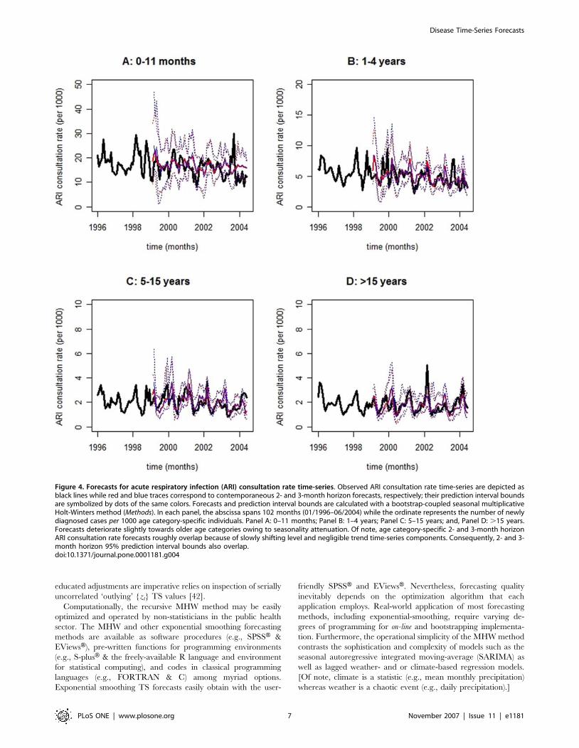
Figure 4. Forecasts for acute respiratory infection (ARI) consultation rate time-series. Observed ARI consultation rate time-series are depicted asblack lines while red and blue traces correspond to contemporaneous 2- and 3-month horizon forecasts, respectively; their prediction interval boundsare symbolized by dots of the same colors. Forecasts and prediction interval bounds are calculated with a bootstrap-coupled seasonal multiplicativeHolt-Winters method (Methods). In each panel, the abscissa spans 102 months (01/1996–06/2004) while the ordinate represents the number of newlydiagnosed cases per 1000 age category-specific individuals. Panel A: 0–11 months; Panel B: 1–4 years; Panel C: 5–15 years; and, Panel D: .15 years.Forecasts deteriorate slightly towards older age categories owing to seasonality attenuation. Of note, age category-specific 2- and 3-month horizonARI consultation rate forecasts roughly overlap because of slowly shifting level and negligible trend time-series components. Consequently, 2- and 3-month horizon 95% prediction interval bounds also overlap.doi:10.1371/journal.pone.0001181.g004



The statistically more sophisticated, and also widely available,

SARIMA model fits disease TS but, not only has it reportedly

failed to consistently produce robust post-sample forecasts for

malaria TS in Abeku et al. [32] but it may also require extensive

user expertise for optimum performance. SARIMA models

require users to iteratively specify SARIMA (p, d, q)(P, D, Q)

components, enforce post differencing stationarity, and test for

residual normality until an acceptable model specification is

achieved. The orders p, d, q, P, D, and Q symbolize the number of

auto-regressive lags, differences, moving-average lags, seasonal

auto-regressive lags, seasonal differences, and seasonal moving-

average lags, respectively. The SARIMA approach not only lacks

a systematic procedure to uniquely specify SARIMA (p, d, q)(P, D,

Q) components but it also requires a minimum of 50 to 100

observations for optimization. Conversely, the MHW forecasting

method implemented herein requires a minimum of 36 TS

Figure 5. Forecasts for malaria consultation rate time-series. Observed malaria consultation rate time-series are depicted as black lines while redand blue traces correspond to contemporaneous 2- and 3-month horizon forecasts, respectively; their prediction interval bounds are symbolized bydots of the same colors. Forecasts and prediction interval bounds are calculated with a bootstrap-coupled seasonal multiplicative Holt-Wintersmethod (Methods). The abscissa spans 102 months (01/1996–06/2004) while the ordinate represents the number of newly diagnosed cases per 1000age category-specific individuals. Panel A: 0–11 months; Panel B: 1–4 years; Panel C: 5–15 years; and, Panel D: .15 years. Forecasts amelioratetowards older age categories owing to seasonality accentuation. Visual inspection suggests a resemblance between ARI (Fig. 4) and malaria time-series, as well as forecasts, for the youngest age category (Panel A: 0–11 months), which might reflect misdiagnosis and or co-morbidity betweenthese two diseases. Clinical diagnosis among infants suffers from two major limitations. Infants are i) immunologically complex and ii) unable toeffectively communicate symptoms. Of note, age category-specific 2- and 3-month horizon malaria consultation rate forecasts roughly overlapbecause of slowly shifting level and negligible trend time-series components. Consequently, 2- and 3-month horizon 95% prediction interval boundsalso overlap.doi:10.1371/journal.pone.0001181.g005



observations plus pseudo-parameter initialization (e.g.,

a= b= c= 0.3) for optimization. This advantage is vital when

available monthly records span 10 years or less, such as the 102

composite monthly disease TS observations that are reported and

analyzed in this manuscript. Unlike SARIMA, however, the

MHW method is not a statistical model since it lacks an error

structure. Hence, PI estimation is herein accomplished via

bootstrapping rather than analytically. More sophisticated state-

space exponential smoothing alternatives [43–46] may surpass the

performance of MHW-based TS forecasts and improve 95% PI

value estimation.

Lagged weather- and or climate-based models are particularly

powerful whenever disease transmission is highly-unstable and

epidemics are suddenly-triggered. A weather-based Poisson re-

gression (4th-degree polynomial distributed lag) model has

successfully forecasted malaria TS in highly unstable regions of

Ethiopia [35]. However, lagged weather- and or climate-based

models not only require extensive programming and user expertise

to reasonably specify the number of lags for each model

component but they also suffer from multicollinearity, problematic

optimization, and lengthy TS requirements. Furthermore, lagged

models, unlike the MHW method, must be tailored to each

disease. While some form of lagged weather- and or climate-based

model may be indispensable [35], the simpler MHW alternative

may forecast fully- or partially-stable disease TS, e.g., meso-

endemic malaria transmission in the district of Niono. Only under

the most unstable transmission conditions should climate and or

weather covariates be invoked to forecast disease TS at specific

locations [32–35]. Weather events must be measured because

predicting its chaotic nature with several weeks in advance is

usually impossible. Predicting climate is not trivial and such

predictions are typically too global to substantially add local

forecasting accuracy [32]. Otherwise, climate-based models have

paramount importance in infectious disease investigations to:

forecast long horizons [48], elucidate complex disease transmission

behavior [34,48], and model infectious disease transmission in the

spatial dimension [36].

Forecasting approaches perform reasonably well whenever

disease transmission comprises relatively large event-probabilities

during (long) investigational periods. Like other forecasting

approaches, the MHW method surrenders when disease trans-

mission depends on rare stochastic events (in highly-structured

populations), each associated with minute (albeit finite) probabil-

ities, governing transient disease dynamics [49]. These highly-

stochastic structured disease dynamics feature sudden epidemic

resurgence and ample epidemic volume variability that are not

easily investigated with univariate and most multivariate methods,

often requiring more sophisticated approaches [e.g., 49].

The major limitation of this investigation concerns missing

monthly records, which are interpolated with monthly median

values from pertinent CSCOM service areas as described in Methods.

A missing monthly record comprises the complete lack of figures for

all diseases and age categories within a single CSCOM service area

and month—i.e., a missing monthly record from a single CSCOM

service area does not imply the simultaneous lack of records for the

other 16 CSCOM service areas. Consequently, results presented

herein carry admonitions concerning: i) the potential bias of

calculated annual consultation rates and dispersion narrowing

(Table 2); as well as, ii) the introduction of TS periodicity.

The potential bias of calculated annual consultation rates

diminish with adoption of median and IQR values to robustly

measure centrality and dispersion, respectively. In the TS context,

records from 3 (from a total of 17) CSCOM service areas are

excluded from analyses (Methods). Disease- and age category-

specific amalgamated TS comprise 14 data sets, each from an

eligible CSCOM service area; hence, a composite monthly TS

observation reflects an aggregate of 14 CSCOM service area

entries. Missing records distribute approximately normally across

Table 3. Multiplicative Holt-Winters method: pseudo-parameter and mean absolute percentage error (MAPE) values.. . . . . . . . . . . . . . . . . . . . . . . . . . . . . . . . . . . . . . . . . . . . . . . . . . . . . . . . . . . . . . . . . . . . . . . . . . . . . . . . . . . . . . . . . . . . . . . . . . . . . . . . . . . . . . . . . . . . . . . . . . . . . . . . . . . . . . . . . . . . . . . . . .

Diseases Age a b c MAPE (%)

h = 2 h = 3

MHW SA3 MHW SA3

Diarrhea 0–11 mo. 0.01 (0.03) ,0.01 (0.16) 0.35 (0.14) 26.6 30.3 25.3 30.1

1–4 yr. 0.01 (0.02) ,0.01 (0.04) 0.32 (0.16) 23.2 30.3 22.8 30.2

5–15 yr. ,0.01 (0.02) 0.02 (0.21) 0.32 (0.17) 42.4 43.3 43.5 44.1

.15 yr. 0.11 (0.19) 0.03 (0.15) 0.23 (0.17) 26.2 32.9 27.0 33.8

ARI 0–11 mo. 0.21 (0.32) ,0.01 (,0.01) 0.24 (0.21) 25.2 25.7 25.0 26.8

1–4 yr. 0.03 (0.07) ,0.01 (0.02) 0.31 (0.19) 22.5 28.2 22.9 30.0

5–15 yr. 0.07 (0.09) ,0.01 (,0.01) 0.30 (0.15) 25.9 25.3 26.3 26.7

.15 yr. 0.23 (0.30) ,0.01 (,0.01) 0.30 (0.20) 24.1 27.1 25.0 30.0

Malaria 0–11 mo. 0.08 (0.09) ,0.01 (,0.01) 0.27 (0.14) 22.9 23.2 22.4 25.9

1–4 yr. 0.18 (0.22) ,0.01 (0.22) 0.24 (0.13) 23.1 28.4 22.9 30.5

5–15 yr. 0.09 (0.09) ,0.01 (0.06) 0.30 (0.16) 22.7 20.9 22.4 23.2

.15 yr. 0.13 (0.08) 0.01 (0.12) 0.26 (0.12) 17.8 17.5 18.1 18.1

Median (and inter-quartile range) pseudo-parameter a, b, and c values—which smooth control level, trend, and seasonal time-series components, respectively—reflectfitting of B = 500 bootstrap-generated full-length pseudo-time-series with the seasonal multiplicative Holt-Winters method. The greater the pseudo-parameter value,the shorter the smoothing memory, i.e., information from the recent-past have more pronounced effects on estimates than those from the distant-past. Generally, thestrength of pseudo-parameters follows c&a$b, which is expected for time-series with highly seasonal and negligible trend components. Furthermore, large meanabsolute percentage error (MAPE) values between observed monthly consultation rates and their median forecasts imply low accuracy and vice-versa. Thus, 92% of the24 time-series (TS) forecasts generated here (2 forecast horizons, 3 diseases, and 4 age categories = 24 TS forecasts) are reasonably accurate, i.e., their MAPE values arecirca 25%. MAPE values from a seasonal adjustment (SA3) forecasting method [32] are also listed for benchmark comparison. The MHW performance is equal or superiorto that of the SA3 forecasting benchmark in 87.5% of the 24 TS forecasts generated here, as implied by equal or smaller MAPE values.doi:10.1371/journal.pone.0001181.t003..

....

....

....

....

....

....

....

....

....

....

....

....

....

....

....

....

....

....

....

....

....

....

.



CSCOM service areas (Shapiro-Wilk normality test: W = 0.9193;

p-value = 0.1436) and approximately uniformly through the in-

vestigational period (Methods). The percentage of missing monthly

records in the amalgamated TS is 13.6 %, generally less than 2%

per year (Methods). The only exception manifests in the, practically

reconstructed, year of 1997 that was employed for program

initialization—nonetheless, this is minimally consequential be-

cause program initialization, otherwise, would reflect the custom-

ary (and arbitrary) ‘opinion of an expert’. Consequently, artificial

TS periodicity introduction subsequent to the interpolation

procedure is highly improbable. Further details on data pre-

processing appear in the Methods section.

ConclusionNotwithstanding the paucity of published MHW-based infectious

disease TS forecasting investigations, these results suggest that the

exceptional forecasting performance of the MHW method in

econometrics and beyond since the 1950s may be capitalized by

the public health sector. The MHW method is operationally

simple, general, reasonably accurate, and available in many

commercially and freely available software and programming

environments. It produces forecasts for very distinct diseases

(diarrhea, acute respiratory infection, and malaria) without

disease-specific tailoring of forecasting method, adapting on-line

to underlying disease TS perturbations. Finally, this method does

not require covariates to forecast diarrhea, acute respiratory

infection, and malaria TS under fully- or partially-stable trans-

mission. Therefore, the MHW method is a strong general-purpose

forecasting method candidate for the aforementioned non-

stationary epidemiological TS. These forecasts could improve

infectious diseases management in the district of Niono, Mali, and

elsewhere in the Sahel.

METHODS

Study settingThis longitudinal retrospective (01/1996–06/2004) TS investiga-

tion is conducted in the district of Niono, Mali (Fig. 1). Panel A in

Fig. 1 is a satellite image that portrays Mali, with a projected

population of 12 million in 2004 [40], along with its neighboring

West-African countries. Panel B corresponds approximately to the

enlarged red demarcation seen in panel A. The district of Niono

(330 km northwest of Bamako, 100 km north of the Niger River,

in the Segou region) is depicted within the red rectangle in panel

B. The district of Niono is a model location to test disease TS

forecast and early warning system feasibility because it shares

epidemiological similarities with other regions in the Sahel where

poverty- and disease-induced morbidity and mortality are

rampant. Additionally, available monthly consultation records

for 20 diseases (including diarrhea, ARI, and malaria) are monthly

resolved in the district of Niono.

Data pre-processingThe review of monthly clinical records is part of a larger study on

climate and health (‘‘Putting climate in the service of public

health’’) that is approved by the ‘‘Columbia University Medical

Center Institutional Review Board’’ (N.Y., U.S.A.) and the ‘‘Ethics

Committee of the Mali National Medical School ’’ (Bamako,

Mali). Patient privacy is secluded from inadvertent (or deliberate)

violations because consultation records comprise monthly sum-

maries that lack information with which individual patients may

be identified. The assembled monthly data set (01/1996–06/2004)

contains consultation records for 20 diseases, which are tabulated

by gender and age category, from 17 CSCOM service areas [39]

within the district of Niono.

However, only data for diarrhea, ARI, and malaria are herein

analyzed beyond frequency description because these diseases

inflict most morbidity and mortality in this district. The national

estimates for age composition are: 4.0% [0–11 months], 15.3%

[1–4 years], 28.1% [5–15 years], and 52.6% [.15 years] [40].

The total projected population (2004) for the district of Niono is

278 741 individuals [39,40]. Consultation records from each

CSCOM service area are adjusted with the annual national

population growth rate of 3.2% [40] before missing records

(Tables 4 & 5) are interpolated by CSCOM-specific monthly

median values.

After adjustment for population growth and missing value

interpolation, age category-specific median annual diarrhea, ARI,

and malaria consultation rates (plus their IQR values) are

calculated for each CSCOM service area to assess age effects on

consultation distributions. These consultation rates are calculated,

and expressed, as the number of newly diagnosed cases per 1000

individuals in an age category during a year. In the TS context, 3

CSCOM service areas are excluded from the TS analyses because

of limited record availability, i.e., these CSCOM TS do not span

the entire investigational period, contain excessive missing

monthly records and hence, do not meet the inclusion criterion

(Table 4): Niono and Nara CSCOM service areas (01/2000–06/

2004) as well as Fassoum CSCOM service area (01/1996–12/

1999). Of note, the Niono CSCOM service area, which includes

the district center and immediate periphery, is one of the 17

CSCOM service areas within the district of Niono. Upon record

exclusion, the considered district population reduces to 208 743

individuals (Table 4). Sequentially, the adjusted monthly consul-

tation records for the remaining 14 (from a total of 17) CSCOM

service areas are amalgamated according to age category and

disease (diarrhea, ARI, and malaria), converted to rates, and then

submitted to TS analyses. TS consultation rates are expressed as

the number of newly diagnosed cases per 1000 individuals in an age

category during a month.

Time-series forecastsThe resulting TS are fitted with the MHW method. The MWH

method is a versatile non-parametric technique (not to be confused

with a statistical model, which has a defined error structure) that

requires neither stationarity nor ‘strict’ linearity to produce

contemporaneous on-line TS forecasts at variable horizons, h

[37,38]. The MHW method adapts to underlying alterations in

disease dynamics and revises its estimates on-line, i.e., with the

accumulation of new observations. This adaptability is essential for

epidemiological forecasting that depends on historical data

because interventions (e.g., prophylaxis and medical treatment)

almost ubiquitously plague longitudinal retrospective TS. Last but

not least, exponential smoothing methods (e.g., MHW) generally

perform better than statistically more sophisticated alternatives

according to a recent forecasting competition, which compared

several forecasting techniques across more than a thousand TS

[50].

The MHW optimizes via minimization of the squared pre-

diction error for the 1-month horizon forecast (h = 1) with

a modified Quasi-Newton non-linear optimization method re-

ferred to as L-BFGS-B, i.e., the limited memory (L) Broyden-

Fletcher-Goldfarb-Shanno (BFGS) method for bounded (B)

variables [51,52]. In Equation 1, F(yt+h|It) is the h-month horizon

forecast for the observed TS {yt} conditioned on the information

set (It) that accumulates until time t; lt and rt are the TS level and

trend components, respectively, as previously defined; and, sm|t–p+h



is the unitless, monthly seasonal factor that is estimated at time t–

p+h (for h#12). The index m = [1,12] reflects the season of the

forecasting horizon h whereas the period p is herein defaulted to

12 months. Possible lower-frequency harmonics, i.e., inter-annual

fluctuations, are handled as level and trend components by the

MHW method because the limited temporal window considered

(01/1996–06/2004) in this investigation precludes stable estima-

tion of oscillations with periods much longer than 12 months.

F (ytzh It)j ~(ltzhgrt)gsm t{pzhj ð1Þ

The MHW method revises estimates recursively as new

observations accumulate ad infinitum with Equations 2, 3, and 4

where a, b, and c are the smoothing pseudo-parameters for lt, rt,

and sm|t, respectively, as defined in the Results section. The MHW

smoothing pseudo-parameters are embedded in recursive

equations (2, 3, and 4) whose roles resemble exponential kernel

smoothing of lt, rt, and sm|t [53].

lt~agyt

sm tj {p

z(1{a)g(lt{1zrt{1) ð2Þ

rt~bg(lt{lt{1)z(1{b)grt{1 ð3Þ

smjt~cgyt

ltz(1{c)gsmjt{p ð4Þ

Table 4. Demographic and consultation record descriptions.. . . . . . . . . . . . . . . . . . . . . . . . . . . . . . . . . . . . . . . . . . . . . . . . . . . . . . . . . . . . . . . . . . . . . . . . . . . . . . . . . . . . . . . . . . . . . . . . . . . . . . . . . . . . . . . . . . . . . . . . . . . . . . . . . . . . . . . . . . . . . . . . . .

CSCOM Population (2004) Time-series period Missing dates Missing months % missing

Boh 7105 01/1996–06/2004 - 0 0.00 (0.00)

Bolibana 18321 01/1996–06/2004 1997 12 0.76 (0.84)

Cocody 6021 01/1996–06/2004 - 0 0.00 (0.00)

Debougou 25603 01/1996–06/2004 1997, 1998 (3) 15 0.94 (1.05)

Diabaly 16974 01/1996–06/2004 1997 12 0.76 (0.84)

Diakiwere 12269 01/1996–06/2004 1999 (3), 2003 (3) 6 0.38 (0.42)

Dogofry 24172 01/1996–06/2004 1997, 1998 (1) 13 0.82 (0.91)

Fassoun 5837 01/1996–12/1999 1997, 1999 (9) 21 1.33 -

Kourouma 8186 01/1996–06/2004 1997, 2001 24 1.52 (1.68)

Molodo 18379 01/1996–06/2004 1997, 2003 (6) 18 1.14 (1.26)

Nampala 7972 01/1996–06/2004 1996 (4), 1997, 1999 (9) 25 1.58 (1.75)

Nara 24161 01/2000–06/2004 2000, 2001, 2002, 2003 (6) 42 2.65-

Pogo 11893 01/1996–06/2004 1997, 2003 (3) 15 0.94 (1.05)

Siribala 22745 01/1996–06/2004 1997, 2001 (3) 15 0.94 (1.05)

Sokolo 14672 01/1996–06/2004 1997, 1999 (3) 15 0.94 (1.05)

Werekela 14431 01/1996–06/2004 1996, 1997 24 1.52 (1.68)

Niono 40000 01/2000–06/2004 2000, 2001 (2), 2002 (1) 16 1.01 -

Total 278741 (208743) 1584 (1428) months - 272 (194) 17.2 (13.6)

The projected number of individuals (2004) served by each community health center (CSCOM) service area within the district of Niono, Mali, is tabulated under thePopulation heading. Potential records are listed under Time-series period. Unavailable CSCOM service area records appear under Missing dates—the number of missingmonthly records for each year is listed in parenthesis otherwise records for the whole year are missing. These are totaled under Missing months and expressed aspercentages from the total number of possible monthly records (across all CSCOM service areas) under the % missing heading. Monthly consultation records from eachCSCOM service area are adjusted with the annual national population growth rate before missing records are interpolated by CSCOM-specific monthly median values.The total projected population (2004) for the district of Niono is 278 741 individuals, growing 3.2% annually according to regional [39] and national [40] estimates. In thecontext of consultation rates, years with more than 6 missing monthly records are excluded from median and inter-quartile-range annual consultation rate calculations.Additionally, inter-quartile-range calculations require records from at least 3 eligible years. In the time-series context, however, the projected district population (2004)reduces from 278 741 to 208 743 individuals upon record exclusion from Fassoum, Nara, and Niono CSCOM service areas—which do not span the entire investigationalperiod and possess excessive missing monthly records. Values that are reported in parenthesis under the headings of Population (2004), time-series period, Missingmonths, and % missing reflect record exclusion from Fassoum, Nara, and Niono CSCOM service areas. After record exclusion, the remaining 14 CSCOM service areascontribute 1428 possible monthly records to the amalgamated time-series, i.e., 14 records per month. Of note, the Niono CSCOM service area, which includes the districtcenter and immediate periphery, is one of the 17 CSCOM service areas within the district of Niono, Mali.doi:10.1371/journal.pone.0001181.t004..

....

....

....

....

....

....

....

....

....

....

....

....

....

....

....

....

....

....

....

....

....

....

....

....

....

....

....

....

..

Table 5. Monthly missing record distribution.. . . . . . . . . . . . . . . . . . . . . . . . . . . . . . . . . . . . . . . . . . . . . . . . . . . . . . . . . . . . . . . . . . . . . . . . . . . . . . . . . . . . . . . . . . . . . . . . . . . . . . . . . . . . . . . . . . . . . . . . . . . . . . . . . . . . . . . . . . . . . . . . . .

Frequency (%)

Year 1996 1997 1998 1999 2000 2001 2002 2003 2004 total

% missing 1.0 (1.1) 9.1 (9.2) 0.3 (0.3) 1.5 (1.1) 1.5 (0.0) 1.8 (1.1) 0.8 (0.0) 1.1 (0.8) 0 (0.0) 17.2 (13.6)

A total of 272 monthly entries are missing from 1584 possible records, accounting for 17.2% of missing data across all community health center (CSCOM) service areas inthe district of Niono, Mali, during the investigational period (01/1996–06/2004). Percentage of missing monthly records after the exclusion of Fassoum, Nara, and NionoCSCOM service areas are listed in parenthesis. The annual percentage of missing monthly records is generally less than 2% per year. The only exception manifests in thepractically reconstructed year of 1997 that was employed for program initialization. Consequently, artificial time-series periodicity introduction subsequent to theinterpolation procedure is highly improbable.doi:10.1371/journal.pone.0001181.t005....

....

....

....

....

....

....

....

....

.



In the simplest case, i.e., in the absence of trend (b= 0) and

periodicity (c= 0), the MHW method reduces to a simple

exponential smoothing filter that has been described in terms of

the Nadaraya-Watson (one-sided) exponential kernel [53]. Other

special cases arise if c= 0 or b= 0, namely when this exponential

method lacks a seasonal or a trend component, respectively. Large

MHW pseudo-parameters confer greater weights to recent in-

formation and effectively shorten the smoothing ‘memory’, i.e., the

recent-past has a more pronounced influence on estimated lt, rt, and

sm|t values than does the distant-past. Fitting is initialized by setting a,

b, and c to 0.3 since their initial choice is trivial—typical and possible

pseudo-parameters are 0,a, b, and c,0.5 and 0,a, b, and c,1,

respectively. Initial values for lt, rt, and sm|t obtain automatically from

a simple moving-average decomposition that employs a minimum of

3 initial TS periods (i.e., 36 months per default), the feasible

specification of additional periods (e.g., p = 4, 5…) notwithstanding

[37,38,52,54]. Forecasts are produced only after 3 TS periods—

subsequent to initialization with the first period p (i.e., the first

12 months) and fitting of the remaining 24 months.

Residual time-series bootstrappingNot only does the MHW method produce accurate forecasts but it

also naturally decomposes {yt} into {lt}, {rt}, {sm|t}, and {zt},

which are shorter than the observed TS by exactly p observations.

However, the lack of an underlying statistical model hinders the

estimation of 95% PI values. Thus, median forecasts and their

empirical 95% PI values are estimated from probability density

functions that are generated at each time t for horizon h by

uniform bootstrapping (B = 500) the approximately serially un-

correlated {zt} TS distribution [55]. The {zt} TS distribution,

which elongates as new observations and their forecasts accumu-

late, is calculated with Equation 5;

fztg~fyt{F (yt It{1)j g ð5Þ

where

fztg*WN(0, s2),

i.e., {zt} is an approximately stationary white-noise process with

mean 0 and variance s2. The first p original TS observations (for

which fitted values are unavailable) are concatenated with shorter

pseudo-TS of length t–p, which are generated via B = 500 {zt} TS

bootstraps and subsequent TS reconstruction with the inverse

function of Equation 5. This ensures that observed TS and

reconstructed pseudo-TS have the same length. The absolute

value of the rare negative monthly pseudo-TS value is enforced

because this forecasting method handles non-negative values only.

Each reconstructed pseudo-TS of length t is fitted with the MHW

method; forecast probability density functions are produced for

h = 2 and h = 3, from which median forecasts and their empirical

95% PI values yield. Quantiles are calculated with p(k) = (k21)/

(n21) via linear interpolation between the kth order statistics and

p(k) where n is the sample size; further information is available in

‘‘R: language and programming environment’’ [52] and references

therein. Reported values for a, b, and c reflect the median and

IQR values of their probability density function upon fitting

B = 500 full-length pseudo-TS.

Forecasting accuracy and precisionForecasting accuracy is calculated as MAPE values between

observed monthly consultation rates and their median forecasts.

The MHW method performance is compared against that of the also

operationally simple SA3 forecasting benchmark, which is recom-

mended in Abeku et al. [32]. SA3 forecasts are generated by

correcting seasonal averages with the mean deviation between the

three most recent seasonal forecasts and their observed TS values

[32] hence, capturing recent TS trend vis-a-vis reducing statistical

variation. Finally, precision is identified with 95% PI values. Large

MAPE (or PI) values imply low accuracy (or precision) and vice-versa.

ACKNOWLEDGMENTSThe authors would like to thank R. Sakai, S. Karambe, D. Konate, N.

Sogoba, M. B. Toure (Malaria Research and Training Center, FMPOS,

Universite de Bamako, Mali) for assistance. This manuscript is dedicated to

Moussa Dembele (District hospital of Niono, Ministry of Health, Niono,

Mali) who deceased during the time of manuscript writing, but who

clinically supervised all 17 community health centers within the district of

Niono during the entire investigational period.

Author Contributions

Conceived and designed the experiments: SF SD. Analyzed the data: DM.

Wrote the paper: DM. Other: Digitalized records: BG. Conducted

preliminary data analyses: BG.

REFERENCES1. Brewster DR, Greenwood BM (1993) Seasonal variation of paediatric

diseases in The Gambia, West Africa. Annals of Tropical Paediatrics 13(2):

133–146.

2. Craig MH, Snow RW, le Sueur D (1999) A Climate-based Distribution Model ofMalaria Transmission in Sub-Saharan Africa. Parasitology Today 15(3):

109–116.

3. National Research Council (2001) Under the weather: climate, ecosystems, and

infectious disease. Washington DC, US: National Academy Press.

4. Tanser FC, Sharp B, le Sueur D (2003) Potential effect of climate change on

malaria transmission in Africa. Lancet 362: 1792–1798.

5. Patz JA, Campbell-Lendrum D, Holloway T, Foley JA (2005) Impact of regional

climate change on human health. Nature 438(7066): 310–317.

6. Lamb P (1978) Large-scale tropical Atlantic surface circulation patterns

associated with Subsaharan weather anomalies. Tellus A30: 240–251.

7. Chambers R, Longhurst R, Pacey A (1981) Seasonal dimensions to rural

poverty. London, Great Britain: Francis Pinter Publisher.

8. Callejas D, Estevez J, Porto-Espinoza L, Monsalve F, Costa-Leon L, et al. (1999)

Effect of climatic factors on the epidemiology of rotavirus infection in children

under 5 years of age in the city of Maracaibo, Venezuela. Investigacion Clinica

40(2): 81–94.

9. Musa HA, Shears P, Kafi S, Elsabag SK (1999) Water quality and public health

in northern Sudan: a study of rural and peri-urban communities. Journal of

Applied Microbiology 87(5): 676–682.

10. Singh RB, Hales S, de Wet N, Raj R, Hearnden M, et al. (2001) The influence

of climate variation and change on diarrheal disease in the Pacific Islands.

Environmental Health Perspectives 109(2): 155–159.

11. Sugaya N, Mitamura K, Nirasawa M, Takahashi K (2000) The impact of winter

epidemics of influenza and respiratory syncytial virus on paediatric admissions to

an urban general hospital. Journal of Medical Virology 60(1): 102–106.

12. Weber MW, Mulholland EK, Greenwood BM (1998) Respiratory syncytial virus

infection in tropical and developing countries. Tropical Medicine and

International Health 3(4): 268–280.

13. Weber MW, Milligan P, Sanneh M, Awemoyi A, Dakour R, et al. (2002) An

epidemiological study of RSV infection in the Gambia. Bulletin of the World

Health Organization 80(7): 562–568.

14. Siritantikorn S, Puthavathana P, Suwanjutha S, Chantarojanasiri T, Sunakorn P,

et al. (2002) Acute viral lower respiratory infections in children in a rural

community in Thailand. Journal of the Medical Association of Thailand

85(suppl 4): S1167–1175.

15. Checon RE, Siqueira MM, Lugon AK, Portes S, Dietze R (2002) Seasonal

pattern of respiratory syncytial virus in a region with a tropical climate in

southeastern Brazil. American Journal of Tropical Medicine and Hygiene 67(5):

490–491.

16. van der Sande MA, Goetghebuer T, Sanneh M, Whittle HC, Weber MW (2004)

Seasonal variation in respiratory syncytial virus epidemics in the Gambia, West

Africa. Pediatric Infectious Disease Journal 23(1): 73–74.



17. Phillips-Howard PA (1999) Epidemiological and control issues related to malaria in

pregnancy. Annals of Tropical Medicine and Parasitology 93(suppl 1): S11–17.18. Guyatt H, Snow R (2001) The Epidemiology and burden of Plasmodium

falciparum-related anemia among pregnant women in sub-saharan africa.

American Journal of Tropical Medicine and Hygiene 64(1, 2 S): 36–44.19. Breman J (2001) The Ears of the Hippopotamus: Manifestations, Determinants,

and Estimates of the malaria burden. American Journal of Tropical Medicineand Hygiene 64(1, 2 S): 1–11.

20. Baird JK, Owusu Agyei S, Utz GC, Koram K, Barcus MJ, et al. (2002) Seasonal

malaria attack rates in infants and young children in northern Ghana. AmericanJournal of Tropical Medicine and Hygiene 66(3): 280–286.

21. Duffy PE, Fried M (2005) Malaria in the pregnant woman. Current Topics inMicrobiology and Immunology 295: 169–200.

22. Bloland PB, Wlliams HA (2002) Malaria control during mass populationmovements and natural disasters. Washington DC, US: National Academy

Press.

23. Adams A (1994) Seasonal Variations in nutritional risk among children incentral Mali. Ecology of Food and Nutrition 33: 93–106.

24. Rice AL, Sacco L, Hyder A, Black RE (2000) Malnutrition as an underlyingcause of childhood deaths associated with infectious diseases in developing

countries Bulletin of the World Health Organization 78(10): 1207–1221.

25. Small J, Goetz SJ, Hay SI (2003) Climatic suitability for malaria transmission inAfrica, 1911–1995. PNAS 100(26): 15341–15345.

26. Connor SJ, Thomson MC, Flasse SP, Perryman AH (1998) Environmentalinformation systems in malaria risk mapping and epidemic forecasting. Disasters

22(1): 39–56.27. Kleinschmidt I, Bagayoko M, Clarke GP, Craig M, le Sueur D (2000) A spatial

statistical approach to malaria mapping. International Journal of Epidemiology

29(2): 355–361.28. Kleinschmidt I, Omumbo J, Briet O, van de Giesen N, Sogoba N, et al. (2001)

An empirical malaria distribution map for West Africa. Tropical Medicine andInternational Health 6(10): 779–786.

29. Gemperli A, Vounatsou P, Kleinschmidt I, Bagayoko M, Lengeler C, et al.

(2004) Spatial patterns of infant mortality in Mali: the effect of malariaendemicity. American Journal of Epidemiology 159(1): 64–72.

30. de Castro MC, Monte-Mor RL, Sawyer DO, Singer BH (2006) Malaria risk onthe Amazon frontier. PNAS 103(7): 2452–2457.

31. Rogers DJ, Randolph SE, Snow RW, Hay SI (2002) Satellite imagery in thestudy and forecast of malaria. Nature 415(6872): 710–715.

32. Abeku TA, de Vlas SJ, Borsboom G, Teklehaimanot A, Kebede A, et al. (2002)

Forecasting malaria incidence from historical morbidity patterns in epidemic-prone areas of Ethiopia: a simple seasonal adjustment method performs best.

Tropical Medicine and International Health 7(10): 851–857.33. Hay SI, Were EC, Renshaw M, Noor AM, Ochola SA, et al. (2003) Forecasting,

warning, and detection of malaria epidemics: a case study. Lancet 361(9370):

1705–1706.34. Teklehaimanot HD, Lipsitch M, Teklehaimanot A, Schwartz J (2004) Weather-

based prediction of Plasmodium falciparum malaria in epidemic-prone regionsof Ethiopia I. Patterns of lagged weather effects reflect biological mechanisms.

Malaria Journal 3: 41.35. Teklehaimanot HD, Schwartz J, Teklehaimanot A, Lipsitch M (2004) Weather-

based prediction of Plasmodium falciparum malaria in epidemic-prone regions

of Ethiopia II. Weather-based prediction systems perform comparably to early

detection systems in identifying times for interventions. Malaria Journal 3: 44.36. Thomson MC, Doblas-Reyes FJ, Mason SJ, Hagedorn R, Connor SJ, et al.

Malaria early warnings based on seasonal climate forecasts from multi-model

ensembles. Nature 439(7076): 576–579.37. Holt CC (1957) Forecasting seasonals and trends by exponentially weighted

moving averages. In O.N.R. Research Memorandum 52, Carnegie Institute ofTechnology.

38. Winters PR (1960) Forecasting sales by exponentially weighted moving averages.

Management Sciences 6: 324–342.39. Division des Services Socio-Sanitaires (1996–2004) Disease statistics for the

district of Niono, Mali.40. USAID (2004) Country health report: Mali.

41. Division des Services Socio-Sanitaires (2005) Disease statistics for the district ofGao, Mali.

42. Burkom HS, Murphy SP, Shmueli G (2007) Automated time series forecasting

for biosurveillance. Statistics in Medicine 26(22): 4202–4218.43. Ord JK, Koehler AB, Snyder RD (1997) Estimation and prediction for a class of

dynamic nonlinear statistical models. Journal of the American StatisticalAssociation 92: 1621–1629.

44. Ord JK, Koehler AB (1990) A Structural Model for the Multiplicative Holt-

Winters Method. Proceedings of the Decision Sciences Institute 555–557.45. Chatfield C, Koehler AB, Ord JK, Snyder RD (2001) A new look at models for

exponential smoothing. The Statistician (Journal of the Royal Statistical Society,Series D) 50: 147–159.

46. Hyndman RJ, Koehler AB, Snyder RD, Grose S (2002) A state space frameworkfor automatic forecasting using exponential smoothing methods. International

Journal of Forecasting 18(3): 439–454.

47. Keiser J, Singer BH, Utzinger J (2005) Reducing the burden of malaria indifferent eco-epidemiological settings with environmental management: a sys-

tematic review. Lancet Infectious Diseases 5(11): 695–708.48. Chaves LF, Pascual M (2006) Climate cycles and forecasts of cutaneous

leishmaniosis, a non-stationary vector-borne disease. PLoS Medicine 3(8):

1320–1328.49. Watts DJ, Muhamad R, Medina DC, Dodds PS (2005) Multiscale, resurgent

epidemics in a hierarchical metapopulation model. PNAS 102(32):11157–11162.

50. Makridakis S, Hibon M (2000) The M3-Competition: results, conclusions andimplications. International Journal of Forecasting 16: 451–476.

51. Byrd RH, Lu R, Nocedal J, Zhu CY (1995) A limited memory algorithm for

bound constrained optimization. SIAM Journal of Scientific Computing 16:1190–1208.

52. R Development Core Team (2004) R: A language and environment forstatistical computing. R Foundation for Statistical Computing, Vienna, Austria:

ISBN 3-900051-07-0, URL http://www.R-project.org.

53. Gijbels I, Pope A, Wand MP (1999) Understanding exponential smoothing viakernel regression. Journal of the Royal Statistical Society 61(Series B): 39–50.

54. Cleveland RB, Cleveland WS, McRae JE, Terpenning I (1990) STL: A seasonal-trend decomposition procedure based on Loess. Journal of Official Statistics 6(1):

3–73.55. Politis DN (2003) The impact of bootstrap methods on time series analysis.

Statistical Science 18(2): 219–230.



Forecasting Non-Stationary Diarrhea, Acute Respiratory ...

Documents

Transcript of Forecasting Non-Stationary Diarrhea, Acute Respiratory ...