arX

iv:p

hysi

cs/0

3010

57v1

[ph

ysic

s.da

ta-a

n] 2

2 Ja

n 20

03

Scaling in Non-stationary time series I

M. Ignaccolo1∗, P. Allegrini2, P. Grigolini1,3,4, P. Hamilton5, B. J. West6

1Center for Nonlinear Science, University of North Texas,

P.O. Box 311427, Denton, Texas, 76203-1427

2 Istituto di Linguistica Computazionale del Consiglio Nazionale delle Ricerche,

Area della Ricerca di Pisa-S. Cataldo,

Via Moruzzi 1, 56124, Ghezzano-Pisa, Italy

3Dipartimento di Fisica dell’Universita di Pisa and INFM Via Buonarroti 2, 56127 Pisa, Italy

4Istituto di Biofisica del Consiglio Nazionale delle Ricerche,

Area della Ricerca di Pisa-S. Cataldo,

Via Moruzzi 1, 56124, Ghezzano-Pisa, Italy

5 Center for Nonlinear Science, Texas Woman’s University,

P.O. Box 425498, Denton, Texas 76204 and

6 Physics Department, Duke University, P.O. Box 90291,

Durham, North Carolina 27708 and US Army Research Office,

Mathematics Division, Research Triangle Park, NC 27709

(Dated: February 2, 2008)

∗ Corresponding Author.

Mailing Address: Center for Nonlinear Science, University of North Texas, P.O. Box 311427, Denton, Texas,

76203-1427 .

Phone: +1 940 565 3280 .

E-mail Address: stellina99@earthlink.net .

1

Abstract

Most data processing techniques, applied to biomedical and sociological time series, are only valid for

random fluctuations that are stationary in time. Unfortunately, these data are often non stationary and

the use of techniques of analysis resting on the stationary assumption can produce a wrong information

on the scaling, and so on the complexity of the process under study. Herein, we test and compare two

techniques for removing the non-stationary influences from computer generated time series, consisting

of the superposition of a slow signal and a random fluctuation. The former is based on the method

of wavelet decomposition, and the latter is a proposal of this paper, denoted by us as step detrending

technique. We focus our attention on two cases, when the slow signal is a periodic function mimicking

the influence of seasons, and when it is an aperiodic signal mimicking the influence of a population

change (increase or decrease). For the purpose of computational simplicity the random fluctuation is

taken to be uncorrelated. However, the detrending techniques here illustrated work also in the case

when the random component is correlated. This expectation is fully confirmed by the sociological

applications made in the companion paper. We also illustrate a new procedure to assess the existence

of a genuine scaling, based on the adoption of diffusion entropy, multiscaling analysis and the direct

assessment of scaling. Using artificial sequences, we show that the joint use of all these techniques yield the

detection of the real scaling, and that this is independent of the technique used to detrend the original signal.

PACS : 05.45.Tp; 05.40.-a; 87.23.Ge

keywords : scaling, multiscaling, diffusion entropy, non-stationary time series, detrending methods.

2

I. INTRODUCTION

Time series analysis is the backdrop against which most theoretical models are developed in the

biomedical and social sciences. The traditional assumption made in the engineering literature, and

subsequently adopted in the biophysical, biological and social sciences, is that the discrete time

series variable ξ (tj) consists of a slowly varying part S (tj) and a randomly fluctuating part ζ (tj) :

ξ (tj) = S (tj) + ζ (tj) . (1)

The slow, regular variation of the time series is called the signal, and the rapid erratic fluctuations

are called the noise. The implication of this separation of effects is that S (t) contains information

about the system of interest, whereas ζ (t) is a property of the environment and does not contain

any information about the system.

The Science of Complexity is making us acquainted with a different perspective. Physiological

and sociological time series invariably contain fluctuations, so that when sampled N times the

data set {ξj}, j = 1, ..., N , appears to be a sequence of random points. Examples of such data

are the interbeat intervals of the human heart [1, 2], interstride intervals of human gait [3, 4],

brain wave data from EEGs [5] and interbreath intervals [6], to name a few, and, of course, the

Texas teen birth data [7] analyzed in the companion paper [8]. From now on, we shall refer to

this paper as paper II. The analysis of the time series in each of these cases has made use of

random walk concepts (see Sec. IIA for the details) in both the processing of the data and in the

interpretation of the results. For example, the variance of the associated random walk, σ2(t), in

each of these cases (and many more) satisfies the property σ2(t) ∝ t2H , where H 6= 1/2 corresponds

to anomalous diffusion. A value of H < 1/2 is interpreted as an antipersistent process in which

a step in one direction is preferentially followed by a reversal of direction. A value of H > 1/2

is interpreted as a persistent process in which a step in one direction is preferentially followed

by another step in the same direction. A value of H = 1/2 is interpreted as ordinary diffusion

in which the steps are independent of one another. This would be compatible with the earlier

mentioned concept of environmental noise. In the science of complexity the fluctuations ξi are

expected to depart from this totally random condition, since they are expected to have memory

and correlation. This memory is manifest in inverse power-law spectra of the form P (ω) ∝ 1/ωβ+1,

where the corresponding correlation function, the inverse transform of the spectrum, is determined

by a Tauberian theorem to be

3

C (t1, t2) ∝ |t1 − t2|β . (2)

Here the power-law index is given by β = 2H − 2. Note that the two-point correlation function

depends only on the time difference, thus, the underlying process is stationary. These properties, as

well as a number of other properties, are discussed for discrete time series by Beran. [9]. Another

important property of complex systems is that the associated random walk is not monofractal. For

instance the heart beat variability has been found to be multifractal [10] as were the interstride

intervals [11, 12]. A more accurate way to define the deviation from ordinary diffusion is ensured

by the scaling property. If the time series is long enough, following the prescription of the pioneer

work of Ref. [13] we can generate a diffusion process out of it. The probability density function

(pdf) of the diffusion process, p(x, t), is expected to satisfy the scaling condition

p(x, t) =1

tδF (

x

tδ). (3)

The deviation from ordinary statistical mechanics, and consequently the manifestation of com-

plexity, takes place through two distinct quantities. The first indicator is the scaling parameter δ

departing from the ordinary value δ = 0.5, which it would have for a simple diffusion process. The

second indicator is the function F (y) departing from the conventional Gaussian form. The first

quantity is usually assessed by measuring the second moment, or the variance, of the distribution

as we did above. This method of analysis is reasonable only when F (y) maintains its Gaussian

form. If the scaling condition of Eq. (3) applies, it is convenient to measure the scaling parameter

δ by the method of Diffusion Entropy (DE) [14, 15, 16, 17, 18, 19, 20] that, in principle, works

independently of whether the second moment is finite or not. The DE method affords many ad-

vantages, including that of being totally independent of a constant bias. Unfortunately, in the

presence of a non-constant bias, the scaling detected by the DE need not indicate the correlations

of the fluctuations, but instead would reflect the influence of the time-dependent bias.

This important fact, the relationship of the scaling index to the bias, brings us back to the

decomposition of the time series into a signal plus noise (see Eq. (1)). We address the theoretical

issues raised by a physical condition where the important information is not contained in what the

engineering literature defines as a signal, but rather in what is usual defined as noise. In other

words, we adopt a perspective where the role of the environment might be that of creating a time-

dependent slow component S(t). In this case S(t) could be an external forcing, due to seasonal

4

periodicity, demographic pressure, or to other causes. In any case, we need to isolate ξ(t) from

S(t), to detect the genuine complexity of the system under study. As we shall show, a process of

analysis made without first establishing this separation might give the impression of a complexity

higher than the real one. This overestimation of the scaling index is caused by the non-stationarity

of the time series and inapplicability of the property of Eq. (2), implicitly assumed by the method

of analysis.

We cannot rule out another important possibility. In complex phenomena the separation of

effects implied by Eq. (1) may no longer be appropriate. The low-frequency, slowly changing,

part of the spectrum may be coupled to, and exchange energy with, the high-frequency, rapidly

varying part of the spectrum; a fact that often results in fractal statistical processes. For these

latter processes the traditional view of deterministic, predictable signal given by the smooth part

of the time series, on which random, unpredictable noise is superimposed, distorts the dynamics

of the underlying process. Although the research work of this paper has been done having in mind

the former perspective, namely that the complexity of the system is of internal origin, and that

the slow component S(t) is an external forcing, that does not affect the internal complexity of

the system under study, its result can be used to asses where the latter perspective applies. For

instance, after separating S(t) from ξ(t) in the most rigorous and objective way possible, we might

observe many complex systems, for instance the teen birth process of many different counties, and

to assess if it is true or not that those characterized by a more intense S(t) might lead to a larger

deviation of ζ(t) from ordinary scaling.

The outline of the paper is as follows. In Section II we provide a concise review of diffusion-

based methods used to asses the scaling properties of a time series, the Diffusion Entropy (DE),

the Second Moment (SM), the Multi-Scaling (MS) analysis and the Direct Assessment of Scaling

(DAS), and a brief review of the Wavelet analysis (WA) and its use to reveal the features of the

signal at different time scales. In Section III, with the help of computer-generated time series, we

discuss how the different diffusion-based methods perceive the addition of a “slow component” to

the fluctuations, how to detrend this component (we introduce two different methods: the wavelet

smoothing and the step smoothing) and how the detrending procedures affect the capability of

recovering the scaling properties of the fluctuations. Section IV addresses the same questions of

Section III, but in the case when a “periodic component” is added to the fluctuations. In Section

V we draw some conclusions.

5

II. ILLUSTRATION OF THE ANALYSIS TOOLS USED IN THIS PAPER

To make this paper as self-contained as possible, we devote this section to a concise review

of the methods of analysis that we use. These methods are the diffusion-based methods, the

Diffusion Entropy (DE), the Second Moment (SM), the Multi-Scaling (MS) analysis and the Direct

Assessment of Scaling (DAS), discussed in Section II A, and the decomposition of the time series

done with the Wavelet Analysis (WA), as illustrated in Section IIB.

A. The diffusion based methods

As mentioned in the Introduction, the theoretical backdrop to our discussion is that we have a

stochastic time series denoted by the function ξ (t) . This time series is used to generate a diffusion

process as follows

x(t) =

∫ t

0ξ(t

′

)dt′

. (4)

Here x(t) is the position occupied by a random walker at time t and the function x(t) is a diffusion

trajectory. Furthermore, it is evident that to create a probability density function (pdf) we need

many diffusion trajectories of the type indicated by Eq. (4), namely, an ensemble of statistically

equivalent trajectories.

The continuum form for the diffusion trajectory leaves us with two main problems. The first

problem is typically that we do not have a continuous time data, in which case the integral in Eq.

(4) is replaced by a sum and the time t is discrete. The scaling property of Eq. (3) is usually

discussed within a continuous-time perspective, but since the data are discrete, some caution must

be exercised in moving from one representation to the other. The second, and even more important

problem, is how to create many statistically equivalent trajectories. This is a delicate issue in time

series analysis, where, in general, it is not possible to have many identical replicas of the system,

with many statistically equivalent series of fluctuations. Typically one has only a single time series.

To solve this problem we use an overlapping windows technique. If t is a discrete time in the interval

[1, N ], we define N − t+ 1 different diffusion trajectories (number of members in the ensemble) in

the following way

xk(t) =

k+t∑

j=k

ξj, k = 1, 2, . . . , N − t+ 1. (5)

6

This corresponds to initiating a “window” (interval) of length t at the data point k, and to ag-

gregating all the data in the sequence ξj. For any window position we sum all the values of the

variable ξj spanned by the window. This procedure is shared by all the diffusion based methods.

Let us now explore, briefly, the different methods based on creating a diffusion process from

data via Eq. (5).

1. Diffusion Entropy (DE) Analysis

The rationale behind the adoption of DE analysis is that, if the pdf of the diffusion process

satisfies Eq. (3), then, regardless of the pdf shape, the Shannon entropy satisfies the following

relationship

S(t) = −

∫

∞

−∞

p(x, t) ln [p(x, t)] dx = A+ δ ln(t), (6)

where A is a constant defined by

A = −

∫

∞

−∞

F (y) ln [F (y)] dy, y =x

tδ. (7)

Therefore the scaling condition of Eq. (3) can be detected by searching for the linear dependence

of the entropy of Eq.(6) on a logarithmic time scale.

In practice, the numerical procedure necessary to evaluate the pdf requires that the x-axis be

divided into cells of a given size, that, in principle, might also depend on the cell position on

the x-axis. We adopt the criterion of assigning to each cell the same size, but we leave this size

time-dependent. For this reason we denote the cell size with the symbol ∆ (t). At any time t, the

size ∆ (t) must be chosen so as to lead to a fair approximation of p (x, t), through the histogram

relation

p (xj, t) ≈Pj

∆ (t). (8)

Here p (xj , t) is the histogram at the value xj, the midpoint of the j-th cell, at time t and Pj is the

fraction of the total number of trajectories found in this cell at time t. The rationale behind the

choice of a time-dependent size for the cell has to do with obtaining a good estimate of the pdf from

the histogram. At early times, when the trajectories are close together, a constant ∆ is adequate

to estimate the ratio Pj/∆. As the trajectories diffuse apart, however, either more trajectories are

7

needed, or a larger ∆ is needed, to provide a reasonable estimate for this ratio. To ensure that

(8) is satisfied at any time we evaluate the standard deviation of the diffusion process, σ (t), and

select the cell size to be a fraction of the standard deviation, ∆ (t) = ǫσ (t) where 0.1 ≤ ǫ ≤ 0.2.

There is some sensitivity to the choice of ǫ, but in the proper range of values in which Eq. (8) is

satisfied, the diffusion entropy

S (t) = −

∫

∞

−∞

p(x, t)ln [p(x, t)] dx ≈ −∑

j

Pj lnPj + ln ∆ (t) (9)

is insensitive to the particular fraction of the standard deviation adopted.

It has to be pointed out that the DE analysis can yield a logarithmic dependence on time even

when the scaling condition of Eq. (3) is not fulfilled. This is the case of the symmetric Levy

walk studied by the authors of [20]. Levy walks [21] are characterized by the fact that the time

for the walker to cover a given distance is proportional to the distance itself. This restriction

generates a diffusion process limited by diffusion fronts moving ballistically. In [20] a case where

the population of the ballistic fronts Ppeaks(t) decrease extremely slowly, Ppeaks(t) ∝ t−β with

0 < β < 1, is examined and in this case the pdf between the ballistic peaks tends to become a

Levy distribution with scaling parameter δ = 1β+1 . Due to the slow decrease to zero of Ppeaks(t),

the diffusion process is bi-scaling (the two scaling parameters being that of Levy for the central

part and the ballistic one for the fronts). The numerical limitation in creating a perfect power law,

makes the DE growing, after a transient, linearly with a slope equal to 1β+1 giving the impression

that the condition Eq. (3) is fulfilled. Therefore, it is convenient to denote the slope of the linear

dependence on the logarithm of time of the DE, with the symbol δde.

2. Second Moment (SM) Analysis

The SM analysis is based on evaluating the standard deviation of the diffusion process

σ(t) =[

< {x(t) − x(t)}2 >]

1

2

, (10)

where x(t) ≡< x(t) > and < . . . > denotes the average over the ensemble of realizations of diffusion

trajectories. If the time series fluctuations have zero mean value, the quantity x(t) vanishes and

Eq. (10) can be written as

σ(t) =

[∫

∞

−∞

x2p(x, t)dx

]1

2

, (11)

8

which is, in fact, the square-root of the second moment of the distribution.

We evaluate the standard deviation from Eq. (10), and we look for a time domain where

σ(t) ∝ tδsm ⇔ ln [σ(t)] ∝ δsm ln(t). (12)

is satisfied. Then, in the time domain for which Eq.(10) is fulfilled, the standard deviation rescales

with the scaling parameter δsm. This scaling does not automatically imply, as mentioned in Section

I, that the proper scaling condition of Eq. (3) is fulfilled.

3. Multiscaling (MS) Analysis

The MS analysis is a generalization of the SM analysis. In fact Eq. (10) is replaced by the

expression

σq(t) = [< |x(t) − x(t)|q >]1

q , (13)

where q is a real number. It is evident that Eq. (10) is recovered from Eq. (13) by setting q = 2.

In case of fluctuations with zero mean value, Eq. (13) reads:

σq(t) =

[∫

∞

−∞

|x|qp(x, t)dx

]1

q

. (14)

If the scaling condition of Eq. (3) holds, we can express (14) as

σq(t) = Bq tδ, (15)

where

Bq =

[∫

∞

−∞

|y|qF (y)dy

]1

q

. (16)

Note that even in the case where F (y) has a long tail with an inverse power law index µ, with

µ < 3, and consequently a divergent second moment, the relation of Eq. (15) holds true, if q < 2.

In the case of fractional Brownian motion [22], the function F (y) is Gaussian, the scaling

exponent, usually called H in this case, in honor of Hurst, is a number in the interval [0, 1] and

σq(t) ∝ tH ∀q ∈] − 1,+∞). (17)

In the case of a Levy flight [23] the function F (y) is a Levy stable distribution of index α [21].

Note that the index α is related to the inverse power-law index of the distribution by the relation

9

α = µ− 1, and that the scaling δ is given in this case by δ = 1/α = 1/(µ − 1). Thus, in this case,

it is straightforward to prove

σq(t) ∝ t1

α ∀q ∈] − 1, α[. (18)

As for the SM analysis we look for a time domain where the fq-th fractional standard deviation

σq(t) rescales with exponent ζ(q), namely

[σq(t)]q ∝ tζ(q) ⇔ ln [(σq(t))

q] ∝ ζ (q) ln(t). (19)

When the scaling condition of Eq. (3) applies: q ζ (q) = δq . In the ideal case where divergent

moments are involved, as we have seen earlier, we should limit our observation to values of q smaller

than a given qmax. In practice, we do the calculation for the entire range of values from q = −1

to q = ∞ (in reality the behavior of σq(t) for very high value of q, q > 10 for example, cannot be

trusted because they are dominated by rare events and therefore subject to the problem of lack

of statistics). This is done because, in real data there are no moment divergences, due to the fact

that time series are of finite length. We, then, plot the calculated ζ(q) as a function of q and see

if a straight line results. The corresponding slope is the genuine value of the scaling parameter δ,

assuming that the scaling condition Eq. (3) applies. Of course, with this technique, as in the case

of the DE analysis, there is no compelling reason to ensure that the resulting scaling parameter

corresponds to a genuine scaling property. If the scaling condition exists, the DE analysis and the

MS analysis detect the real scaling parameter (a property that the SM analysis does not share).

The reverse is not necessarily true.

4. Direct Assessment Scaling (DAS)

The definition of scaling given by Eq. (3) has an attractive physical meaning. Given any two

times t2 and t1, with t2 > t1, the pdf at time t2 coincides with the pdf at time t1 if the the following

self-affine transformation is applied: take the scale of the variable x, and “squeeze” it by a factor

R = [t1/t2]δ, simultaneously take the scale of the distribution intensity, and “enhance” it by the

factor 1/R. In other words, when Eq. (3) is satisfied, the diffusion process is invariant under this

self-affine transformation. This property is the expression of a kind of thermodynamic equilibrium

reached by the complex system under study; one that is different from that usually obtained if δ 6=

0.5 and F (y) is not Gaussian. The DAS analysis consists exactly of this procedure of “squeezing”

and “enhancing” aimed at establishing the invariance of the pdf by a scaling transformation.

10

The reader might wonder why no significant use is made of the DAS in literature. The reason

seems to be that the detection of real scaling would necessitate many trials before discovering the

right scaling index, if it exists. We think that the adoption of the DAS only becomes useful after

the DE and MS methods are applied. In fact, those analysis define a possible candidate for the

true scaling. However, these techniques, as we have seen, do not provide any compelling reason to

prove that the resulting scaling is a genuine property of the system dynamics. Herein, we apply

the DE and the MS analysis and use the DAS to check if we have determined a genuine scaling or

not.

B. Wavelet Analysis (WA)

The wavelet transformation [24, 25] is close in spirit to the Fourier transformation, but has a

significant advantage. The Fourier transformation decomposes a time series into a superposition

of oscillating modes, each of which lasts forever. The wavelet transformation decomposes the time

series into “notes” or wavelets [25], localized in time and in frequency. Formally, the wavelet

transform f(s, t) of the function f(u) is defined as follows

f(s, t) ≡

∫ +∞

−∞

du : |s|−pψ∗(u− t

s)f(u), (20)

where the symbol ψ∗ denotes the complex conjugate of the wavelet ψ(u). The wavelet ψ(u) is a

filter function satisfying the particular condition, known as the “admissibility condition” [24, 25].

The parameters s, t and p, are real numbers. Eq. (20) shows the advantages of the wavelet

transformation in resolving local features of the time series. In fact, the wavelet transformation

rests on a convolution of the signal with the wavelet rescaled, through the use of the parameter

s, and centered on u = t. Therefore the parameter s localizes the frequency domain and the

parameter t localizes the time domain.

Herein we use the discrete version of the wavelet transformation, known as the Maximum

Overlap Discrete Wavelet Transform (MODWT) that gives birth to a decomposition of the signal

in terms of “approximations” and “details” relative to different time scales. Consider the integers

N and K. The former is the length of the series under study and K is the greatest number

satisfying the condition 2K < N . In this condition we can consider K different time scales, given

by 21, 22, . . . , 2K . Then, starting from the smallest time scale, the wavelet transformation is used

to divide the original time series S into two components

S = A1 +D1. (21)

11

The component A1 contains features having a characteristic time scale greater than 21, since a

local average of the time series over all time scales inferior to 21 has been performed. Therefore

the component A1, often referred as “approximation”, is “21-smooth”, in the sense that A1 can

be considered a slow changing function with respect the time scale 21. The component D1, on the

other hand, contains all the features of the time series with a characteristic time scale less than 21

and therefore is called the “detail”. The partitioning procedure described above can then applied to

the approximation A1, splitting it into the functions A2 and D2. The latter two functions represent,

respectively, the features of the time series with time scales greater than 22 and those features with

a time scale less than 22, but greater than 21, that have already been removed. Clearly, at the k-th

step of this procedure, with k < K, we have the decomposition

S = Ak +Dk +Dk−1 + . . .+D1, (22)

with Ak representing the smooth time series referring to the time scale 2k and Dj, with 1 < j < k,

the detail of time series with the time scale located in the interval [2k−1, 2k].

III. COMPUTER-GENERATED DATA: EFFECTS OF A SLOW COMPONENT

In Section I we mentioned that the main goal of this paper is to detect the scaling index as a

measure of complexity of time series: this task is confounded by the presence of slow components.

In this section we illustrate the influence of a slow component on a computer-generated random time

series created for this specific purpose. We apply the diffusion entropy (DE), the second moment

(SM), the multiscaling analysis (MS) and the direct assessment scaling (DAS) analysis to this

computer-generated time series, and establish that it is not possible to reach a reliable conclusion

about the real complexity of the process with any of these techniques. Consequently we show how

to eliminate the influence of the slow component, without distorting the scaling properties of the

fluctuations, if any exists. This detrending procedure aims at establishing a stationary condition,

to which DE, SM and MS analysis can be productively applied.

Let us introduce the computer-generated time series we use to test the above processing tech-

niques. We adopt a discrete-time picture, so that the time series to analyze reads as follows:

ξj = STj + ζj, (23)

where both STj and ζj are functions of the discrete time j. The slow component of the time

series, STj , is a function, either regular or stochastic, that changes over a long time scale denoted

12

by T . The function ζj represents the fluctuations and we refer to it as noise. In the numerical

calculations, we assume the noise to not have any memory. However, the conclusion reached in this

section can be easily extended to the case where ζj has a long-time memory, yielding a scaling index

δ moderately larger than the simple diffusion scaling, δ = 0.5. We shall consider three different

kinds of slow components, all of them with zero mean: a linear drift with a small slope, SLTj , a

slowly changing continuous function, SCTj , and a step function, SST

j . Fig. 1 shows these three

different slow components. We select ζ to be a Gaussian random process with zero average and

standard deviation σ = 12, to which we will refer as Gaussian noise (GN). This choice of σ makes

the intensity of the GN, measured by the standard deviation, comparable to the intensity of the

slow components SCTj and SST

j , while keeping the noise at a slightly larger intensity than that of

the SLTj component.

We note that DE analysis applied to the computer-generated time series, corresponding to GN,

is a perfectly straight line, with δ = 0.5. The use of random, rather than correlated, fluctuations

in the simulation is dictated by simplicity. This choice of a memoryless noise makes the non-

stationary effects, produced by the slowly changing first term on the right-hand side of Eq. (23),

more transparent. However, the theoretical arguments adopted, in the remaining part of this

section, to explain these significant effects, are independent of whether the noise is memoryless or

correlated. Finally, the length, 13149, of the data has been chosen for ease of application of these

results in paper II.

A. Diffusion Entropy (DE) and Second Moment (SM) Analysis

In this section we apply the DE and the SM analysis to the computer-generated sequences of

Eq. (23). Figs. 2 and 3 illustrate the DE and the SM methods, respectively. In both figures the

top, middle and bottom frame refer to SSTj , SCT

j and SLTj , respectively. In each frame we compare

the results relative to the application of the methods to the time series defined by the sum of the

slow component and the GN, as in Eq. (23), with the results obtained when the two components

are considered separately.

Regarding the slow components SSTj and SCT

j , we see from Fig. 2 that at short times the DE

generated by the time series of Eq. (23), is different from both the DE of the slow component and

the DE of the GN component. This is explained by the fact that the slow component and GN have

comparable intensities. Thus, it is evident that their joint action generates a faster spreading of the

pdf and therefore a faster entropy increase. At long times the joint action of the two components

13

yields the same effects as the slow component alone. This is due to the fact that the slow component

generates ballistic diffusion, which is faster than the simple diffusion generated by the GN alone.

A different behavior appears with the slow component SLTj . In this case, the short-time behavior

is dominated by the noise component. This dominance by the noise occurs because the intensity

of this component is smaller than the noise intensity. However, even in this case the long-time

behavior is dominated, as explained earlier, by the slow component. This is a remarkable property,

because in this case a mere visual inspection of the time series is not sufficient to reveal the

presence of a bias, which is hidden by very large fluctuations. In any event, the adoption of the DE

method yields a large scaling exponent that one might erroneously attribute to highly correlated

fluctuations. This is an effect that we have to take into account when analyzing real time series.

The SM analysis reveals properties similar to those emerging from the DE analysis, the only

relevant difference is that the convergence to the steady condition of the slow component alone is

much faster than in the corresponding case of the DE analysis. It is worthwhile to discuss this

result in detail. Let us define σtot(t) as the total standard deviation, at a time t, of the diffusion

process relative to the sum of the slow component and the noise. Under the assumption that the

individual components of the signal of Eq. (23) are independent of one another, we write

σ2tot(t) = σ2

slow(t) + σ2noise(t) = σ2

slow(t)

[

1 +σ2

noise(t)

σ2slow(t)

]

. (24)

The SM analysis rests on evaluating the increase with time of the logarithm of the standard

deviation. With some elementary algebra, we convert Eq. (24) into

log [σtot(t)] = log [σslow(t)] +1

2log

[

1 +σ2

noise(t)

σ2slow(t)

]

. (25)

When the noise standard deviation is smaller than the slow component standard deviation, namely,

σnoise(t) ≪ σslow(t), using the Taylor series expansion of the logarithm. we obtain

log [σtot(t)] ≈ log [σslow(t)] +1

2

σ2noise(t)

σ2slow(t)

. (26)

Therefore, when σnoise(t) ≪ σslow(t) the leading contribution of the SM analysis is the logarithm

of the slow component standard deviation, and the next expansion term is the square of the ratio

of the noise standard deviation to the slow component standard deviation. In the case of diffusion

entropy the numerical results indicate that a plausible expression to use is

Stot(t) = Sslow(t) +O

[

σnoise(t)

σslow(t)

]α

, (27)

14

with α < 2. In fact, the numerical results illustrated in the frames of Fig. 2 corresponding to

SCTj and SST

j reveal that the diffusion entropy is more sensitive to the noise component than is the

SM analysis. This sensitivity is due to the convergence to the behavior dominated by the slow

component being faster than the one relative to the SM analysis. For a deeper understanding of

the diffusion created by the superposition of the noise and slow component, in the next subsection

we use the multiscaling analysis.

B. Multiscale (MS) Analysis

In Fig. 4 we observe that in the long-time limit, t > 100, the DE produced by the time series

resulting from the sum of noise and slow component SSTj coincides with the DE generated by

the slow component alone that increases with a slope equal to 1. This asymptotic property has

already been discussed. Our goal here is to shed light on the convergence to the long-time scaling

of the whole time series, with the help of multiscaling analysis. To accomplish this goal, we divide

the time range, explored by the DE analysis, into three time regions: times smaller than 10 (early

stage of the diffusion process), times between 10 and 100 (middle stage of the diffusion process) and

times from 100 to 1000 (later stage of the diffusion process). We apply the multiscaling analysis

to the two time series in Fig. 4, for each of these three time regions, as shown in Fig. 5.

The three frames of Fig. 5, from bottom to top refer to the early, the middle and the later

stage of the diffusion process, respectively. The squares denote the numerical results relative to

the slow component alone, the triangles denote the numerical results concerning the sum of slow

component and noise and the dashed line corresponds to a straight line of slope 1, as expected

for a diffusion rescaling ballistically. Moving from the bottom to the top we notice that the

agreement between triangles and squares tend to increase. At the top, there is an almost complete

equivalence throughout the whole q-region explored. We also see that in the early and middle

region the disagreement between triangles and squares tend to increase upon increasing q. This

means that the difference between the two cases becomes more and more significant at larger and

larger distances. The presence of noise tends to slow down the distribution broadening.

To understand the influence of the GN on the slow component, we notice that the position of

any of the diffusing trajectories can be written at time t as

x(t) = xslow(t) + xnoise(t), (28)

where the contributions to x(t) are separated into the slow component and noise, respectively.

15

Now, since the noise has a vanishing mean, we have 50% probability that the absolute value of

x(t) is increased by the presence of the noise and 50% that it is decreased. When we raise the

absolute value of x(t) to a power of q larger than 1, the half with positive increment contribute to

the q-th moment with a greater weight than the other half. So, at any given time, the presence of

the noise component makes the q-th moments , with q > 1, larger than in the case without noise,

namely, the larger q, the larger the discrepancy. We know that at long times, the moments of the

two distributions, those with and without noise, must coincide. As earlier pointed out, this occurs,

because the noise component has slower diffusion. Consequently, the moments of the distribution

with noise undergo a slower increase than the moments of the distribution without noise.

C. Direct Assessment Scaling (DAS)

Finally, we want to use the DAS method to shed light on the apparently confusing situation

emerging from the use of DE, SM, and MS analysis. We have seen that the DE suggests that

δ = 0.86 might be a reasonable measure of scaling, thereby suggesting the existence of pronounced

cooperation in the system under study. The MS method, on the contrary, suggests that the

ballistic scaling, δ = 1, is a more appropriate representation of the system complexity, at least in

the long-time regime. Using the DAS we discover that neither of these two conditions is a proper

representation of the system dynamics. Previously, we studied three distinct time regimes, short,

intermediate and long. Here we focus on the intermediate time regime, ranging from 10 to 100.

This choice is dictated by the fact that the deviation from a straight line in the middle frame of

Fig. 4 suggests that the DE prediction of δ = 0.86 is questionable.

We apply the DAS method, namely, the squeezing and enhancing technique, assuming for the

scaling parameter δ, the values 1, 0.86 and 0.6. The corresponding results are illustrated in the top,

middle and bottom frames of Fig. 6, respectively. We see that the adoption of δ = 1 leaves the tail

and the peak positions unchanged. However, the peak intensity (in particular the intensity of the

central peak) is not invariant. This lack of invariance of the peaks means that δ = 1 is an acceptable

scaling parameter for the skeleton of the pdf and its tail, but not for the peak′s intensities. The

adoption of δ = 0.86, as suggested by the DE analysis, is satisfactory for both peak intensities

and position. However, this scaling property is limited to the central part of the histogram. We

see from the middle frame of Fig. 6 that the choice of the scaling parameter indicated by DE has

difficulty with the side portions of the histogram. In fact, we see that the peak at x = −200 is

annihilated by the adoption of the DAS method. Finally, as we see in the last panel, the scaling

16

parameter δ = 0.6 turns out to be unsatisfactory everywhere.

In summary, the scaling parameter δ = 0.86 emerging from DE analysis depicted in Fig. 4 does

not reflect the true scaling of the computer-generated process. Fig 6 indicates that the scaling

δ = 0.86, afforded by DE, refers to the central part of the distribution, whereas the sides of the

histogram are more satisfactorily represented by the scaling δ = 1. This is reminiscent of the

multiscaling properties revealed, using the MS analysis , in the paper of Ref. [20]. However, in

the case studied in Ref. [20] the scaling of the central part, corresponding to Levy walk dynamics,

turned out to be a fair reflection of the correlated nature of fluctuations. Here, this anomalous

scaling is not the effect of correlated fluctuations, rather it is the consequence of the non-stationary

effects produced by the slow component superposed on the GN with our computer-generated data.

D. Detrending the Slow Component

The above results establish that a slow component can produce misleading effects that have to

be removed in order to detect the scaling properties of stationary fluctuations. The possible corre-

lations remaining after the slow component has been removed, indicate the amount of cooperation

of the system. In the following subsections we illustrate two distinct detrending methods, the “step

smoothing” and “wavelet smoothing“.

1. Step Smoothing

The “step smoothing” procedure consists of dividing the time series into non-overlapping patches

of length equal to the characteristic time T : we evaluate the average value inside each patch and

we subtract it from the data. In other words, this procedure consists of approximating the slow

component with a step function of the same kind as that of the top frame of Fig.1. The details of

the procedure are as follows. Start from Eq. (23) and create the new variable Xj, the sum of the

variable ζ inside the j-th patch, namely,

Xj =

k<(j+1)T∑

k=jT

ξk j = 0, 1, 2, .., P, (29)

where P is the number of patches of length T in the time series. To make explicit the contribution

to Xj of the two components (the slow and the random) of the variable ξj we define

17

Rj =

k<(j+1)T∑

k=jT

ζk j = 0, 1, 2, ..., P (30)

Aj =

k<(j+1)T∑

k=jT

STk j = 0, 1, 2, ..., P (31)

and therefore

Xj = Aj +Rj. (32)

If it happens that in any single patch the second term of the right-hand side of Eq. (32) is negligible

compared to the first term, we can use this equation to evaluate the average of the slow component

and consider it as a fair approximation to the slow component inside each patch. Moreover, we

notice that the noise component has zero mean. Thus, the most probable value for Rj is zero,

and the error associated with this prediction is given by the standard deviation σRj, therefore

Rj = 0 ± σRj. Then, using the definition Eq. (30) we apply the following approximation

σRj≈ σ0 T

δsm , (33)

where σ0 is the standard deviation of the variable ζ and the exponent δsm is a number between

0 and 1. If the scaling condition applies and the standard deviation is finite, this exponent is the

scaling coefficient, that is, δsm = δ. If the scaling condition does not apply, this exponent is given

by the mean slope. Finally, with the help of Eq. (33) we can state that Xj ≈ Aj when

σ0 Tδsm ≪ |aj| T ⇒ σ0 ≪ |aj | T

1−δsm , (34)

where aj is the average amplitude of the slow component in the j-th patch, and, with this equation

holding true,

aj ≈Xj

T(35)

In Fig. 7 we show the results of this detrending procedure for the three time series with the three

slow components of Fig. 1, with characteristic time T = 365 and with GN. We choose the value

365 in anticipation of the application of these techniques to yearly data in paper II. We see that

the slow components SSTj and SCT

j (top and middle frame of Fig. 7) are fairly well reproduced,

while the result for the slow component SLTj (bottom frame of Fig. 7) is poor. The reason for

18

this behavior is that the first two cases satisfy the condition of Eq. (34) while the last one does

not. In fact, in the last case the absolute value of the average, |aj |, relative to the j-th patch is

considerably smaller than σ0, the intensity of the GN.

2. Wavelet Smoothing

Another way of obtaining an approximation to the slow component is to use the chain of

approximations and details stemming from the MODWT. If T is the characteristic time of the slow

component, a good approximation is given by the j-th wavelet approximation, the one relative to

scale 2j where j is such that 2j is as close as possible to the time T (T = 365, so both j = 8 and

j = 9 are good choices). In fact, the wavelet transformation acts as a filter on the contributions

corresponding to time scales smaller than the time scale examined. The detrending procedure rests

on eliminating the component corresponding to the T -time scale from the data.

We apply the wavelet smoothing to the three time series that have been analyzed, in Fig. 7, by

means of the step detrending procedure. Our purpose is to show that the two detrending techniques

yield virtually the same results. We choose as analyzing wavelet the Daubechies wavelet number

1 and 8, the same as those adopted elsewhere [26]. We denote these wavelets as db1 and db8,

respectively. We adopt, as a scale, 29 = 512. The results are shown in Figs. 8 and 9, respectively.

In both cases, as expected, we get results very similar to what obtained with the step procedure.

This means that the wavelet method very satisfactorily reproduces both the SSTj and SCT

j (top

and middle frame) time series, but it turns out to be as inaccurate as the step detrending method,

and very similar as well, when applied to the SLTj time series (bottom frame). This equivalence

is a consequence of the wavelet result retaining, in part, the features of the mother wavelet, which

is, in turn, a square wave. The adoption of the db8 wavelet yields a result that is as inaccurate as

that of wavelet db1 and the step detrending method.

3. The Effects of the Detrending Procedure

We are, now, in a position to check a crucial step of our approach to the search of the complexity

of a given process. In the next section we shall show how to detrend a periodic bias. When this

approach is applied to real sequences in paper II, we derive a time series similar to the slow com-

ponent plus noise that we are discussing here. Then, we shall have to detrend the slow component

using the procedure of this subsection. For the sake of simplicity, the computer-generated time

19

series, here under study, has been chosen to be the sum of a slow component and uncorrelated fluc-

tuations. Consequently, in the case here under study the fluctuations emerging from the adoption

of the detrending procedure should be random, therefore yielding δ = 0.5.

Now we apply the DE method to the time series resulting from the detrending procedures and

assess the extent we succeed in recovering the statistical properties of the GN. We consider three

time series resulting from the addition of GN to the three slow components SSTj , SCT

j and SLTj .

In Fig. 10 we apply the step smoothing detrending and in Figs. 11 and 12 we use the wavelets db8

and db1, respectively. We notice that in all three cases the detrending procedure works very well,

if we ignore the saturation taking place at long times. The remainder of this subsection is devoted

to explaining why the detrending procedure is affected by the unwanted saturation effect.

Let us first direct our attention to the results in Fig. 10, the case of the step smoothing

procedure, and why the saturation effect is an artifact of the detrending procedure. Using Eq. (35)

it can be shown that the detrended time series (variable ξ) is obtained from the original time series

according to the following prescription

ξk = ξk −∑

j

(

Πjk

Xj

T

)

, (36)

where Πjk is the characteristic function of the j-th patch. Using (23) and Eq. (32), it is possible to

write

ξk = ζk + STk −

∑

j

(

Πjk

Aj

T

)

−∑

j

(

Πjk

Rj

T

)

. (37)

We recall that different diffusing trajectories are created using the method of overlapping windows.

According to this method, the position occupied at time t by the m-th trajectory, denoted by

Γξ(m, t), is given by

Γξ(m, t) =

k=m+t−1∑

k=m

ξk. (38)

The right-hand side of Eq. (37) is the sum of four contributions, and, correspondingly, the right-

hand side of Eq. (38) can be expressed as the sum of four terms. These terms are, with, obvious

notations, Γζ(m, t), ΓST (m, t), ΓA(m, t) and ΓR(m, t). Therefore Eq. (38) can be written as

Γξ(m, t) = Γζ(m, t) + ΓST (m, t) − ΓA(m, t) − ΓR(m, t). (39)

At this point we can determine the reason for the saturation effect. In fact, when the index m

denotes the beginning of a patch and t = T , the function Γξ(m, t), being the sum of ξ within

20

the patch, vanishes (see the definition of Rj and Aj in Eq. (30)). For values of m denoting a

position different from the first site of a patch, the quantity Γξ(m, t) can assume non-vanishing

values. However, the above mentioned constraint establishes an upper bound on Γξ(m, t), thereby

reducing the spreading of diffusion process. As we can see from Fig. 10, the reduction of the

diffusion process is already significant at times smaller than T . Consequently, the step detrending

procedure successfully detrends for only a limited range of times, which we estimate to be t < T3 .

The wavelet method yields saturation effects for similar reasons. In fact using the wavelet

method we detrend the j-th approximation (2j & T ), and the j-th approximation is obtained

through a filtering process averaging all the components with a time scale smaller than 2j . There-

fore, this procedure is similar to the step smoothing, and the ensuing saturation effects have the

same origin.

Finally, we notice that the step smoothing is slightly more effective than the wavelet db8 smooth-

ing in the case of the step component SSTj , while in the case of the continuous component SCT

j

it is the other way around. In fact, the nature of the two signals SSTj and SCT

j is such that the

step smoothing is naturally the best “fit” for SSTj and the db8 wavelet smoothing is naturally the

best one for SCTj . Therefore, in the case of the step smoothing acting on SCT

j , the detrending

process in not so successful and its effect occur before saturation, becoming thus visible. The same

argument applies to the db8 wavelet smoothing acting on SSTj , thereby explaining why the db1

wavelet smoothing does not produce excellent results when applied to both SSTj and SCT

j (top

and middle frame of Fig. 12. Finally, in the case of the SLTj all the detrending procedures do

not work effectively, given the fact that in this case the noise intensity is much greater than the

slow-component intensity.

IV. COMPUTER-GENERATED DATA: EFFECTS OF A PERIODIC COMPONENT

In this section we analyze, again with the help of computer-generated sequences, the effects of a

periodic component rather than the slow components. This is another issue of crucial importance

for the analysis of data sets with strong annual periodicities. The effects of this kind of external

bias have been previously studied in Refs. [16, 19]. The task of this section is, of course, that of

proving that the detrending of a periodic component is a necessary step toward the detection of

the true scaling of the underlying phenomenon with the diffusion based methods of analysis, DE,

SM, MS and DAS.

We use the same notation as that of Eq. (23), and we describe the signal to analyze in this

21

section as

ξj = ΦTj + ζj, (40)

where ΦTj is a periodic function, of period T , satisfying the relation

k<(j+1)T∑

k=j

Φk = 0 ∀j. (41)

Eq. (41) yields the vanishing of the mean value of function Φj. As in the case studied in the previous

Section, the presence of the seasonal component has the effect of “masking” the scaling properties

of the diffusion process stemming from the variable ζ, by producing additional spreading. However,

due to the fact that the external bias is periodic, the additional spreading undergoes regression to

the initial condition at times that are an integer multiple of the period T . This yields an alternating

sequence of increasing and decreasing spreading phases. For this reason we refer to the diffusion

effect caused by the periodic component as the “accordion” effect.

For a convenient explanation of the “accordion” effect, let us study the variable Γξ(j, t). As in

the previous section, the quantity t is the length of the window (or diffusion time) and j is the

initial position of the sliding window. In the present case Γξ(j, t) reads

Γξ(j, t) =

k=j+t−1∑

k=j

(

ΦTk + ζk

)

= ΓΦT (j, t) + Γζ(j, t). (42)

By noticing that

t = nT + τ, (43)

with n being a given integer depending on t and τ, a real number between 0 and T , and by using

Eq. (41), we obtain

Γξ(j, t) = ΓΦT (j + nT, j + nT + τ) + Γζ(j, t). (44)

Now, with t and therefore τ fixed, as the index j runs along the sequence the function ΓΦT (j +

nT, j + nT + τ) repeats itself every T steps and inside this time period the function assumes a

maximum and a minimum value. The difference between these two extremes is a measure of the

spreading due to the seasonal component. It is evident that if τ = 0, that is, if t is a multiple of

the period T , the “seasonal” spreading is zero. With τ increasing, the spreading increases, but

then it has, eventually, to decrease since for τ = T the initial condition must be recovered. Using

22

Eq. (42) or Eq. (44) it is evident that if we want to know the scaling property of the diffusion

relative to the variable ζ alone, we have to look at the diffusion relative to the variable ξ only at

times t that are multiples of the period T , since for these times, we have

Γξ(j, t) = Γζ(j, t) (45)

throughout the whole sequence. So, in principle, there would be no reason to process the data in

any way in order to retrieve the desired information on the variable ζ. We might, in fact, limit

ourselves to studying the behavior of the DE or SM at times that are a multiple of T . However,

when dealing with real data, the limitation on the number of data points available and the excessive

magnitude of T limits the accuracy of the observation of times that are multiples of the time period.

For example if the number of data is 13149 and T = 365 (the case study in paper II), then the

saturation effect, due to lack of statistics, affects the DE or SM already at times smaller than 2T .

Therefore if we want insight into the properties of the diffusion process of the noise component,

before any saturation takes place, we must detrend the periodic component from the time series.

Let us proceed with the detrending in this case. Consider a time series whose length is NT , N

being an integer. In other words, we assume the sequence to have a length which is a multiple of

the time period T . We define

Σξ(j) =

N−1∑

m=0

ξj+mT = NΦj +

N−1∑

m=0

ζj+mT (46)

for all the values of j ∈ [0, T ], or, in a more concise notation,

Σξ(j) = NΦj + Σζ(j) j ∈ [0, T ] . (47)

Eq. (47) can be used to evaluate the periodic component Φj if Σζ(j) ≪ NΦj. Using the same

argument as that adopted earlier for the detrending of the slow component. We establish the

condition

σ0 Nδ ≪ N ΦT

j ⇔ σ0 ≪ ΦTj N1−δ, (48)

yielding

ΦTj ≈

Σξ(j)

N. (49)

23

We note a significant difference with respect to the case of the moving window that we are

forced to adopt in the general case. In this case the detrended data do not show any saturation

effect. In fact

ξj = ζj −1

N

N−1∑

m=0

ζj+mT , (50)

does not vanish if the sum of ξj is carried out over a patch.

In Fig. 13 we illustrate the results of a test done with a periodic function and a computer-

generated sequence having GN. The first frame of Fig. 13 shows the periodic component used

and the one resulting from the detrending procedure described above, the agreement is good. The

second frame depicts the diffusion entropy applied to the sequence with both noise and periodic

component, to the sequence with only the noise component and to the sequence derived from

the detrending procedure. The agreement between the DE applied to the original noise and the

DE applied to the detrended sequence is impressive, and, as expected, there is no indication of a

saturation effect.

V. CONCLUDING REMARKS

We have shown that the DE method, although possessing the remarkable property of detecting

genuine scaling if it exists, cannot be trusted in general as method for detecting the true scaling

index. In fact, the existence of scaling makes the diffusion entropy grow in direct proportion to the

logarithm of time. However, if the diffusion entropy grows in direct proportion to the logarithm of

time, this growth is not necessarily an indication that the rate of this logarithmic increase is the

scaling parameter. It is possible that there is no scaling [20]. Nevertheless, the adoption of the DE

method is useful, since it allows us to determine very quickly the range of values over which the

scaling parameter may be located. At that stage the determination of the correct scaling value of

the scaling parameter has to be determined using a more fine grained analysis, based on the MS

analysis and the DAS. In paper II [8] we shall see this method at work in a case of sociological

interest.

MI and PG gratefully acknowledge financial support from the Army Research Office Grant

DAAD 19-02-0037. PH acknoledges support from NICHD grant R03

[1] B.J. West, R. Zhang, A.W. Sanders, J.H. Zuckerman and B.D. Levine, Phys. Rev. E 59, 3492 (1999).

24

[2] C.-K. Peng, J. Mietus, J. M. Hausdorff, S. Havlin, H. E. Stanley, and A. L. Goldberger , Phys. Rev.

Lett. 70, 1343 (1993).

[3] J.M. Hausdorff, C.K. Peng, Z. Ladin, J.Y. Wei and A.L. Goldberger, J. Appl. Physiol. 78, 349 (1995).

[4] B.J. West and L. Griffin, Fractals 6, 101 (1998).

[5] B.J. West, M.N. Novaes and V. Kavcic, Chapter 10 in Fractal Geometry in Biological Systems, Eds.

P.M. Iannoccone and M. Khokha, CRC, Boca Raton (1995).

[6] H.H. Szeto, P.Y. Cheng, J.A. Decena, Y. Cheng, D. Wu and G. Dywyer, Am. J. Physiol. 262 (Regu-

latory Integrative Comp. Physiol. 32) R141 (1992).

[7] B.J. West, P. Hamilton and D.J. West, Fractals 7, 113 (1999).

[8] M. Ignaccolo, P. Allegrini, P. Grigolini, P. Hamilton and B. J. West, submitted to Physica A.

[9] J. Beran, Statistics for Long-Memory Processes, Chapman & Hall, New York (1994).

[10] P.C. Ivanov, L.A.N. Amaral, A.L. Goldberger, S. Havlin, M.G. Rosenblum, Z.R. Struzik and H.E.

Stanley, Nature 399, 461 (1999).

[11] J.M. Hausdorff, S.L. Mitchell, R. Firtion, C.K. Peng, M.E. Cudkowicz, J.Y. Wei and A.L. Goldberger,

J. Appl. Physiol. , 262 (1997).

[12] L. Griffin, D.J. West and B.J. West, J. Biol. Phys. 26, 185 (2000).

[13] C.-K. Peng, S.V. Buldyrev, S. Havlin, M. Simons, H.E. Stanley and A.L. Goldberger, Phys. Rev. E 49,

1685 (1994).

[14] N. Scafetta, P. Hamilton, and P. Grigolini, Fractals 9, 193 (2001).

[15] P. Grigolini, L. Palatella, and G. Raffaelli, Fractals 9, 439 (2001).

[16] P. Allegrini, P. Grigolini, P. Hamilton, L. Palatella, G. Raffaelli and M. Virgilio, in Emergent Nature,

Ed. M.M. Novak, World Scientific, pp. 173 (2002).

[17] P. Allegrini, P. Grigolini, P. Hamilton, L. Palatella, G. Raffaelli and M. Virgilio, Phys. Rev. E 65,

041926-1-5 (2002).

[18] P. Grigolini, D. Leddon and N. Scafetta, Phys. Rev. E 65, 046203-1-13 (2002).

[19] P. Allegrini, V. Benci, P. Grigolini, P. Hamilton, M. Ignaccolo, G. Menconi, L. Palatella, G. Raffaelli,

N. Scafetta, M. Virgilio and J. Yang, to appear in Chaos, Solitions & Fractals

[20] P. Allegrini, J. Bellazzini, G. Bramanti, M. Ignaccolo, P. Grigolini and J. Yang, Phys. Rev. E 66,

015101 (R) (2002)

[21] J. Klafter, M.F. Shlesinger and G. Zumofen, Phys. Today 49(2), 33 (1996); Lect. Notes in Phys. 519,

15 (1998).

[22] B.B. Mandelbrot, The Fractal Geometry of Nature, Freeman, New York (1983).

[23] B.V. Gnedenko and A.N. Kolmogorov, Limit Distributions for Sums of Independent Random Variables,

Addison-Wesley, Cambridge, MA (1954).

[24] D.B. Percival and A.T. Walden, Wavelet Methods for Time Series Analysis, Cambridge University

Press, Cambridge (2000).

[25] G. Kaiser, A Friendly Guide to Wavelets, Birkhauser, Boston (1994).

25

[26] N. Scafetta, P. Hamilton, P. Grigolini and B.J.West, Phys. (condmat) 0208117

26

FIG. 1: The three different slow components adopted. From the top to the bottom frame: step function,

continuous smooth function and straight line with a small slope. The initial value of the straight line is −2

and the final, at a time t = 13149, is 2.

27

FIG. 2: The diffusion entropy, S(t), as a function of time t, in a logarithmic scale. Each frame shows

three different curves, concerning noise, solid line, slow component , dashed line, and sum of noise and slow

component, dotted line. As far as the slow component is concerned, from the top to the bottom frame

we illustrate the results concerning SSTJ , SCT

J , and SLTJ , namely the slow components illustrated in the

corresponding frames of Fig. 1.

28

FIG. 3: The logarithm of the standard deviation, ln(σ(t)), as a function of time t, in a logarithmic scale.

Each frame contains a set of three curves, the full line referring to the noise alone, the dashed line to the

slow component alone and the dotted line to the sum of slow component and noise. From the top to the

bottom frame these sets of curves refer to SSTJ , SCT

J and SLTJ , respectively. These are the slow components

of the top, middle and bottom frame of Fig. 1, respectively.

29

FIG. 4: The diffusion entropy S (t) as a function of the logarithm of time. The squares denote the time

series corresponding only to the slow component SSTj and the triangles denote the slow component SST

j

plus noise (bottom frame of Fig. 2). We note that the two straight lines suggest that in the time range from

10 to 100 the former and the latter curves correspond to δ = 0.86 and δ = 1, respectively.

30

FIG. 5: The exponent ξ(q) as a function of the parameter q. The squares and the triangles denote the results

of the MS analysis applied to the slow component alone and to the the sum of the slow component and

noise, respectively. The three frames refer, from the top to the bottom to the short-time region, betwenn 1

and 10, the middle-time region, betwen 10 and 100, and the large-time scale, between 100 and and 1000.

31

FIG. 6: The DAS analysis of the time series given by the sum of the slow components SSTj plus the GN.

We consider the middle-time region, defined in Section III B. On the axis of the ordinates ρ (x) we plot the

histograms produced by adopting different squeezing and enhancing transformations, described in Section

III C, to assess to what extent the various histograms coincide. The three frames refer, from top to bottom,

to DAS analysis with the scaling parameter, δ = 1, 0.86 and 0.6, respectively.

32

FIG. 7: The step smoothing technique of Section III D 1 at work. With the full line we indicate the results

of the step smothing procedure, and with the dashed line the slow component to derive. From the top to

the bottom frame we refer to the case where the slow component are SSTj , SCT

j and ST Tj , resspectively .

33

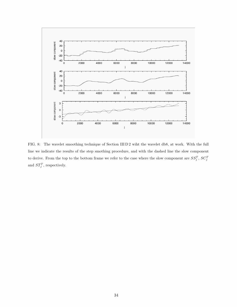
FIG. 8: The wavelet smoothing technique of Section III D 2 wiht the wavelet db8, at work. With the full

line we indicate the results of the step smothing procedure, and with the dashed line the slow component

to derive. From the top to the bottom frame we refer to the case where the slow component are SSTj , SCT

j

and ST Tj , respectively.

34

FIG. 9: The wavelet smoothing technique of Section III D 2 wiht the wavelet db1, at work. With the full

line we indicate the results of the step smothing procedure, and with the dashed line the slow component

to derive. From the top to the bottom frame we refer to the case where the slow component are SSTj , SCT

j

and ST Tj , respectively.

35

FIG. 10: The diffusion entropy, S(t), as a function of time t, in a logarithmic time scale. The triangles

denote the results of the DE analysis applied to the series produced only by the noise component. The

dashed line refers to the DE applied to the sum of noise and slow component. The dotted line denotes

the results of the detrending procedure. From top to bottom the three frames refere SSTj , SCT

j and SLTj ,

respectively. The detrending mehod used is the step smoothing procedure

36

FIG. 11: The diffusion entropy, S(t), as a function of time t, in a logarithmic time scale. The triangles

denote the results of the DE analysis applied to the series produced only by the noise component. The

dashed line refers to the DE applied to the sum of noise and slow component. The dotted line denotes

the results of the detrending procedure. From top to bottom the three frames refere SSTj , SCT

j and SLTj ,

respectively. The detrending mehod used rests on the wavelet db8.

37

FIG. 12: The diffusion entropy, S(t), as a function of time t, in a logarithmic time scale. The triangles

denote the results of the DE analysis applied to the series produced only by the noise component. The

dashed line refers to the DE applied to the sum of noise and slow component. The dotted line denotes

the results of the detrending procedure. From top to bottom the three frames refere SSTj , SCT

j and SLTj ,

respectively. The detrending mehod used rests on the wavelet db1.

38

FIG. 13: Top frame: The periodic component as a function of the linear time. The full lines denotes the real

component and the squares the results of a procedure based on the use of Eq.(49). Bottom frame: diffusion

entropy S(t) as a function of time t in a logarithmic time scale. The triangles denotes the result of the DE

analysis applied to the noise component alone. The full line illustrates the result of the DE analysis applied

to the time series stemming from the sum of noise and periodic component. The dashed line refers to the

the results of the DE applied to the signal resulting from the detrending procedure of Section IV A.

39