Ship design and optimizationA scaling procedure for modern propeller designs

VI International Conference on Computational Methods in Marine Engineering MARINE 2015

F. Salvatore, R. Broglia and R. Muscari (Eds)

A SCALING PROCEDURE FOR MODERN PROPELLER DESIGNS

DR. STEPHAN HELMA*

* Stone Marine Propulsion Ltd (SMP) Dock Road, Birkenhead, Merseyside, CH41 1DT, United Kingdom

e-mail: sh@smpropulsion.com, www.smpropulsion.com

Key words: Scale Effects, ITTC 1978 Power Prediction, Lerbs-Meyne, Strip Method, Open-Water Efficiency

Abstract. The extrapolation procedures currently used to scale propeller characteristics tested at model scale to their full scale performances are either based on a statistical [1], the Lerbs-Meyne [2] or the recently developed strip method [3].

With the emergence of so-called unconventional propellers and different design strategies associated with them, it has been questioned whether the assumptions used in these scaling methods are still universally valid. E.g. with tip and root unloading employed, the circulation distribution deviates from the optimum, which is assumed by the Lerbs-Meyne method; more modern profiles show a different camber distribution and hence the drag coefficient must be aligned with the hydrodynamic inflow angle and not with the pitch to diameter ratio as assumed by the strip method (and implicitly by the ITTC 1978 method [4]).

The work presented still uses the assumption of the equivalent profile and will explain a modified scaling procedure showing a way to calculate the hydrodynamic inflow angle solely from one open-water test conducted at a constant Reynolds number. Finally exemplary results comparing a propeller of conventional type with a recent propeller designs will also be shown.

The new proposed method shows a superior performance when compared to other scaling methods.

1 INTRODUCTION

In recent years new propeller design philosophies have emerged into the market. The NPT-, Kappel- and CLT-propellers are examples of these so-called unconventional designs. From the very beginning it was claimed by their designers that full scale predictions based on the existing scaling methods do not reflect the actual performances observed. Based on the data available to the author this holds true for at least one of the above mentioned propeller types: The trial results regularly show a performance above the speeds predicted by different model basins. Generally speaking this behaviour never posed a problem in the past. With everybody now looking for the most efficient configuration, more and more propellers are comparatively tested and the final design is decided on the outcome of the performance predictions. Some propeller manufactures even take the scaling procedure used at the model basin into their consideration when designing a propeller for a comparative test to gain a little advantage over competitors. These tests pose a complete new challenge to the model basins, since tiny

1051

Dr. Stephan Helma

2

differences – often as small as 0.01 kn – determine who wins the contract. This shows clearly that a more accurate scaling procedure is in high demand.

2 EXISTING SCALING PROCEDURES Currently four main scaling procedures are used in model basins to scale the measured open-

water data to full scale propeller performance: 1. No scaling 2. ITTC 1978 extrapolation method 3. Lerbs-Meyne method 4. Strip method Independently of the scaling method applied, there are some local preferences in the

implementation of the open-water tests, mainly concerning the Reynolds number used. Some model basins adheres strictly to the ITTC recommendation that the Reynolds number “must not be lower than 2·105 at the open-water test” [4] (some of them just fulfilling the recommendation running the open-water test at a Reynolds number of 2·105); some model basins conduct two tests (one at the Reynolds number experienced during the self-propulsion test and one above 2·105, using the lower to analyse the self-propulsion test, the other to scale to the full scale open-water curve); at least one model basin arranges for three open-water tests (one at the Reynolds number of the self-propulsion and two higher ones “to assess if the flow is fully turbulent”). If just one open-water test is conducted, it might or might not be scaled down to the Reynolds number experienced at the self-propulsion test.

2.1 No scaling When predicting the full scale performance, the open-water test is not extrapolated to full

scale, but a final correction factor is applied to the performance prediction.

2.2 ITTC 1978 extrapolation method The ITTC 1978 extrapolation method assumes a linear correlation between the change in

friction drag and change in thrust and torque coefficient [4]. But “it should be kept in mind that both the relation between thrust/torque and drag coefficient and the relation between drag coefficient and Reynolds number are based on statistics and the basis for the statistical values is very small” [1]. This very clear warning should always be kept in mind when judging the accuracy of any results using this extrapolation method. With the emergence of new profile types this warning becomes more and more vehemently – especially when comparing propellers using different profile types.

The second problematic characteristics of this scaling method is the linear dependence of the change in the thrust coefficient on the pitch to diameter ratio 𝑃𝑃/𝐷𝐷. To explain the impact of this assumption, let us consider a propeller with a flat camber line and compare it to one, where all the lift is generated by camber alone. The first propeller will have a higher pitch because the lift is only generated by the angle of incidence. Even if this propeller will perform worse than the cambered one, it will be favoured by the extrapolation method and might show a scaled performance superior to the second, cambered propeller.

The ITTC 1978 extrapolation method insists to test the propeller model at a Reynolds

1052

Dr. Stephan Helma

3

number “not […] lower than 2·105 at the open-water test” [4]. If you compared the performance extrapolated from open-water tests conducted at different Reynolds numbers you want to get the same values independently from the starting point. The left picture in figure 2 shows three full scale open-water curves of the same propeller but scaled up from different Reynolds numbers according to ITTC. Evidently the curve calculated from the lowest Reynolds number does not coincide with the other two curves despite the fact that the lowest Reynolds number of about 2.5·105 is well above the ITTC 1978 recommendation of 2·105. The propeller shown in the right picture in figure 2 exhibits an even worse behaviour: There is a big difference in the extrapolated performances depending on the starting point. The first propeller tested was of a Wageningen B type, the second was of the modern NPT type. Both propellers were tested at the same model basin.

2.3 Lerbs-Meyne method The Lerbs-Meyne method was published in 1968 [2] and derives a propeller with optimum

distribution of circulation and no friction, that is the ideal propeller, from the open-water test at one Reynolds number. With an assumed drag ratio 𝜀𝜀0.7 of the so called equivalent profile at radius 0.7𝑅𝑅, the measured values 𝜂𝜂 and 𝑐𝑐𝑇𝑇𝑇𝑇, the open-water efficiency and the thrust coefficient, respectively, can be converted to 𝜂𝜂𝑖𝑖 and 𝑐𝑐𝑇𝑇𝑇𝑇𝑖𝑖 of the ideal propeller. However there is only one valid combination of 𝜂𝜂𝑖𝑖 and 𝑐𝑐𝑇𝑇𝑇𝑇𝑖𝑖 which can be read of the Kramer diagram [5]. Most likely the calculated 𝜂𝜂𝑖𝑖(𝜀𝜀0.7) and 𝑐𝑐𝑇𝑇𝑇𝑇𝑖𝑖(𝜀𝜀0.7) do not coincide with the valid combination, so 𝜀𝜀0.7 has to be adjusted in an iterative process until the valid combination is met. The full scale values are calculated with a friction coefficient of 0.006.

The Lerbs-Meyne method seems to be the perfect scaling method, since the profile drag is calculated from the actually measured open-water values and it is aligned with the inflow. There are only two drawbacks. Firstly, it is based on an equivalent profile which represents the whole propeller blade. Secondly, it assumes that the propeller blade was designed with an optimum circulation distribution. This poses a problem with modern propellers which are almost always wake adapted designs. The designer also often unloads the tip or root region or the diameter is restricted, so the assumption of optimum circulation distribution does not hold for all designs.

The figure 3 shows the scaled open-water tests.

2.4 Strip method The strip method was developed by H. Streckwall of the HSVA model basin and published

in 2013 [3]. When analysing the open-water test, the vector sum of the contributions of each radial section (strip) towards the friction resistance is calculated to get the friction resistance of the whole blade. When doing so, it takes into account the actual Reynolds number and the position of the transition point at the respective radial strip.

The strip method is certainly an advancement of the existing scale methods. The advantages are that it accounts for the actual turbulence in the inflow, e.g. in open-water and behind condition, by using two different friction lines. It also takes into account the actual distribution of chord length and pitch. The main problems are the alignment of the drag forces with the nose-tail pitch line instead of the actual inflow angle (see the respective note in section 2.2 about the ITTC 1978 extrapolation procedure) and the determination of the friction coefficients. As pointed out by Streckwall the calculation of the friction coefficient uses the local friction

1053

Dr. Stephan Helma

4

coefficients for laminar and turbulent flow as stated by Hoerner [6] and the location of the transition point is derived from CFD calculations. These calculations were done for a set of propellers for two inflow conditions: One with low turbulence for the open-water curve, one with higher turbulence for the behind condition as expected during self-propulsion tests. Final curve fittings result in the two friction resistance curves for the open-water and the behind condition. These derived curves are used for all propellers disregarding of the actual profile used, whereas it is to be expected that the location of the transition point is strongly influenced by the section shape.

The scaled open-water tests can be found in figure 4.

3 ALTERNATIVE SCALING METHOD In the author's opinion a scaling method which is independent of the propeller geometry can

only be realized if the drag coefficient is not parallel to the nose-tail pitch line but aligned with the hydrodynamic inflow as the theory of thin profiles suggests. We will see in the following chapters that it is possible to calculate the hydrodynamic inflow angle from just one open-water test.

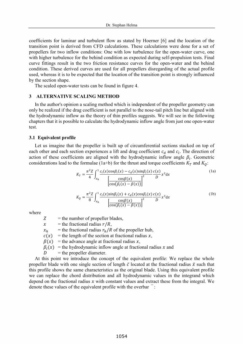
3.1 Equivalent profile Let us imagine that the propeller is built up of circumferential sections stacked on top of

each other and each section experiences a lift and drag coefficient 𝑐𝑐𝑑𝑑 and 𝑐𝑐𝑙𝑙. The direction of action of these coefficients are aligned with the hydrodynamic inflow angle 𝛽𝛽𝑖𝑖. Geometric considerations lead to the formulae (1a+b) for the thrust and torque coefficients 𝐾𝐾𝑇𝑇 and 𝐾𝐾𝑄𝑄:

𝐾𝐾𝑇𝑇 = 𝜋𝜋2𝑍𝑍4 ∫ 𝑐𝑐𝑙𝑙(𝑥𝑥)cos𝛽𝛽𝑖𝑖(𝑥𝑥) − 𝑐𝑐𝑑𝑑(𝑥𝑥)sin𝛽𝛽𝑖𝑖(𝑥𝑥)

[ cos𝛽𝛽(𝑥𝑥)cos(𝛽𝛽𝑖𝑖(𝑥𝑥) − 𝛽𝛽(𝑥𝑥))]

2𝑐𝑐(𝑥𝑥)𝐷𝐷 𝑥𝑥2d𝑥𝑥

1

𝑥𝑥ℎ

(1a)

𝐾𝐾𝑄𝑄 = 𝜋𝜋2𝑍𝑍8 ∫ 𝑐𝑐𝑙𝑙(𝑥𝑥)sin𝛽𝛽𝑖𝑖(𝑥𝑥) + 𝑐𝑐𝑑𝑑(𝑥𝑥)cos𝛽𝛽𝑖𝑖(𝑥𝑥)

[ cos𝛽𝛽(𝑥𝑥)cos(𝛽𝛽𝑖𝑖(𝑥𝑥) − 𝛽𝛽(𝑥𝑥))]

2𝑐𝑐(𝑥𝑥)𝐷𝐷 𝑥𝑥3d𝑥𝑥

1

𝑥𝑥ℎ

(1b)

where 𝑍𝑍 = the number of propeller blades, 𝑥𝑥 = the fractional radius 𝑟𝑟/𝑅𝑅, 𝑥𝑥ℎ = the fractional radius 𝑟𝑟ℎ/𝑅𝑅 of the propeller hub, 𝑐𝑐(𝑥𝑥) = the length of the section at fractional radius 𝑥𝑥, 𝛽𝛽(𝑥𝑥) = the advance angle at fractional radius 𝑥𝑥, 𝛽𝛽𝑖𝑖(𝑥𝑥) = the hydrodynamic inflow angle at fractional radius 𝑥𝑥 and 𝐷𝐷 = the propeller diameter. At this point we introduce the concept of the equivalent profile: We replace the whole

propeller blade with one single section of length 𝑐𝑐̅ located at the fractional radius �̅�𝑥 such that this profile shows the same characteristics as the original blade. Using this equivalent profile we can replace the chord distribution and all hydrodynamic values in the integrand which depend on the fractional radius 𝑥𝑥 with constant values and extract these from the integral. We denote these values of the equivalent profile with the overbar ̅ :

1054

Dr. Stephan Helma

5

𝐾𝐾𝑇𝑇 = 𝜋𝜋2𝑍𝑍4

𝑐𝑐𝑙𝑙cos𝛽𝛽𝑖𝑖 − 𝑐𝑐𝑑𝑑sin𝛽𝛽𝑖𝑖

[ cos𝛽𝛽cos(𝛽𝛽𝑖𝑖 − 𝛽𝛽)

]2

𝑐𝑐𝐷𝐷∫ 𝑥𝑥2d𝑥𝑥

1

𝑥𝑥ℎ

(2a)

𝐾𝐾𝑄𝑄 = 𝜋𝜋2𝑍𝑍8

𝑐𝑐𝑙𝑙cos𝛽𝛽𝑖𝑖 + 𝑐𝑐𝑑𝑑sin𝛽𝛽𝑖𝑖

[ cos𝛽𝛽cos(𝛽𝛽𝑖𝑖 − 𝛽𝛽)

]2

𝑐𝑐𝐷𝐷∫ 𝑥𝑥3d𝑥𝑥

1

𝑥𝑥ℎ

(2b)

(For an alternative formulation of the equivalent profile, which takes the distribution of the chord length and pitch into account, see [7].)

Note that for the equivalent profile the thrust and torque coefficients must remain the same as for the whole propeller blade, hence the overbar ̅ can be omitted.

After integration the equations (2a+b) become:

𝐾𝐾𝑇𝑇 = 𝜋𝜋2𝑍𝑍4

𝑐𝑐𝑙𝑙cos𝛽𝛽𝑖𝑖 − 𝑐𝑐𝑑𝑑sin𝛽𝛽𝑖𝑖

[ cos𝛽𝛽cos(𝛽𝛽𝑖𝑖 − 𝛽𝛽)

]2

𝑐𝑐𝐷𝐷1 − 𝑥𝑥ℎ3

3 (3a)

𝐾𝐾𝑄𝑄 = 𝜋𝜋2𝑍𝑍8

𝑐𝑐�̅�𝑙sin𝛽𝛽𝑖𝑖 + 𝑐𝑐𝑑𝑑cos𝛽𝛽𝑖𝑖

[ cos𝛽𝛽cos(𝛽𝛽𝑖𝑖 − 𝛽𝛽)

]2

𝑐𝑐𝐷𝐷1 − 𝑥𝑥ℎ4

4 (3b)

and finally

𝐾𝐾𝑇𝑇 = 𝜘𝜘𝑇𝑇𝛣𝛣2(𝑐𝑐𝑙𝑙cos𝛽𝛽𝑖𝑖 − 𝑐𝑐𝑑𝑑sin𝛽𝛽𝑖𝑖) (4a)

𝐾𝐾𝑄𝑄 = 𝜘𝜘𝑄𝑄𝛣𝛣2(𝑐𝑐𝑙𝑙sin𝛽𝛽𝑖𝑖 + 𝑐𝑐𝑑𝑑cos𝛽𝛽𝑖𝑖) (4b)

using the following abbreviations for convenience:

𝜘𝜘𝑇𝑇 =𝜋𝜋2𝑍𝑍4

𝑐𝑐𝐷𝐷1 − 𝑥𝑥ℎ3

3 (4c)

𝜘𝜘𝑄𝑄 = 𝜋𝜋2𝑍𝑍8

𝑐𝑐𝐷𝐷1 − 𝑥𝑥ℎ4

4 (4d)

𝜘𝜘 = 𝜘𝜘𝑄𝑄𝜘𝜘𝑇𝑇

= 381 − 𝑥𝑥ℎ41 − 𝑥𝑥ℎ3

(4e)

𝛣𝛣 =cos(𝛽𝛽𝑖𝑖 − 𝛽𝛽)

cos𝛽𝛽

(4f)

Furthermore the advance angle �̅�𝛽 is known for a given advance coefficient 𝐽𝐽:

tan𝛽𝛽 = 𝑣𝑣0𝜔𝜔𝑟𝑟 =

𝐽𝐽𝜋𝜋𝑥𝑥

(4g)

The theory of aerofoils states that the lift coefficient 𝑐𝑐�̅�𝑙 does not change with the Reynolds number [8]. We can (reasonably) assume that if the lift does not change, the induced velocities

1055

Dr. Stephan Helma

6

will not change either, hence the hydrodynamic inflow angle �̅�𝛽𝑖𝑖 does not change with the Reynolds number for any given value of 𝐽𝐽, hence the coefficient 𝛣𝛣 and the lift coefficient 𝑐𝑐�̅�𝑙 stay constant for a fixed 𝐽𝐽-value. This assumption will certainly hold true as long as no flow separation occurs:

Let us recapitulate the dependencies on the advance coefficient 𝐽𝐽, the fractional radius �̅�𝑥 and the Reynolds number Rn̅̅̅̅ of the equivalent profile of each variable:

𝑐𝑐̅ = 𝑐𝑐̅(�̅�𝑥) 𝐾𝐾𝑇𝑇 = 𝐾𝐾𝑇𝑇(𝐽𝐽, Rn̅̅̅̅ ) 𝐾𝐾𝑄𝑄 = 𝐾𝐾𝑄𝑄(𝐽𝐽, Rn̅̅̅̅ ) 𝑐𝑐�̅�𝑑 = 𝑐𝑐𝑑𝑑(𝐽𝐽, Rn̅̅̅̅ , �̅�𝑥) 𝑐𝑐�̅�𝑙 = 𝑐𝑐𝑙𝑙(𝐽𝐽, �̅�𝑥) �̅�𝛽 = �̅�𝛽(𝐽𝐽, �̅�𝑥) �̅�𝛽𝑖𝑖 = �̅�𝛽𝑖𝑖(𝐽𝐽, �̅�𝑥) 𝜘𝜘𝑇𝑇 = 𝜘𝜘𝑇𝑇(�̅�𝑥) 𝜘𝜘𝑄𝑄 = 𝜘𝜘𝑄𝑄(�̅�𝑥) 𝜘𝜘 = const 𝛣𝛣 = 𝛣𝛣(𝐽𝐽, �̅�𝑥)

3.2 Determination of the hydrodynamic inflow angle �̅�𝜷𝒊𝒊 from just one open-water test

The thrust and torque coefficients 𝐾𝐾𝑇𝑇 and 𝐾𝐾𝑄𝑄 depend on the advance coefficient 𝐽𝐽 and the Reynolds number Rn̅̅̅̅ :

𝐾𝐾𝑇𝑇 = 𝐾𝐾𝑇𝑇(𝐽𝐽, Rn̅̅̅̅ ) (5a)

𝐾𝐾𝑄𝑄 = 𝐾𝐾𝑄𝑄(𝐽𝐽, Rn̅̅̅̅ ) (5b)

Traditionally these equations are looked at with the Reynolds number Rn̅̅̅̅ fixed resulting in the well-known open-water curves 𝐾𝐾𝑇𝑇(𝐽𝐽)|Rn̅̅̅̅ , 𝐾𝐾𝑄𝑄(𝐽𝐽)|Rn̅̅̅̅ . If the same propeller were tested at different Reynolds numbers, the three-dimensional surfaces 𝐾𝐾𝑇𝑇(𝐽𝐽, Rn̅̅̅̅ ) and 𝐾𝐾𝑄𝑄(𝐽𝐽, Rn̅̅̅̅ ) can be constructed. Cutting these surfaces at constant 𝐽𝐽-values result in the open-water curves 𝐾𝐾𝑇𝑇(Rn̅̅̅̅ )|𝐽𝐽 and 𝐾𝐾𝑄𝑄(Rn̅̅̅̅ )|𝐽𝐽 depending only on the Reynolds number. Omitting |𝐽𝐽, which indicates that the 𝐽𝐽-value is fixed, for clarity, equations (4a+b) are written for fixed values of 𝐽𝐽 as

𝐾𝐾𝑇𝑇(Rn̅̅̅̅ ) = 𝜘𝜘𝑇𝑇𝛣𝛣2[𝑐𝑐𝑙𝑙cos𝛽𝛽𝑖𝑖 − 𝑐𝑐𝑑𝑑(Rn̅̅̅̅ )sin𝛽𝛽𝑖𝑖] (6a)

𝐾𝐾𝑄𝑄(Rn̅̅̅̅ ) = 𝜘𝜘𝑄𝑄𝛣𝛣2[𝑐𝑐𝑙𝑙sin𝛽𝛽𝑖𝑖 + 𝑐𝑐𝑑𝑑(Rn̅̅̅̅ )cos𝛽𝛽𝑖𝑖] (6b)

We can isolate the lift and drag coefficients 𝑐𝑐�̅�𝑙 and 𝑐𝑐�̅�𝑑(Rn̅̅̅̅ ):

𝛣𝛣2 𝑐𝑐𝑙𝑙 = 𝐾𝐾𝑄𝑄(Rn̅̅̅̅ )sin𝛽𝛽𝑖𝑖

𝜘𝜘𝑄𝑄+ 𝐾𝐾𝑇𝑇(Rn̅̅̅̅ )

cos𝛽𝛽𝑖𝑖𝜘𝜘𝑇𝑇

(7a)

𝛣𝛣2 𝑐𝑐𝑑𝑑(Rn̅̅̅̅ ) = 𝐾𝐾𝑄𝑄(Rn̅̅̅̅ )cos𝛽𝛽𝑖𝑖

𝜘𝜘𝑄𝑄− 𝐾𝐾𝑇𝑇(Rn̅̅̅̅ )

sin𝛽𝛽𝑖𝑖𝜘𝜘𝑇𝑇

(7b)

We differentiate the first equation (7a) with respect to the Reynolds number Rn̅̅̅̅

1056

Dr. Stephan Helma

7

0 = d𝐾𝐾𝑄𝑄

dRnsin𝛽𝛽𝑖𝑖𝜘𝜘𝑄𝑄

+ d𝐾𝐾𝑇𝑇

dRncos𝛽𝛽𝑖𝑖𝜘𝜘𝑇𝑇

(8)

and multiply by dRn̅̅̅̅

0 = d𝐾𝐾𝑄𝑄sin𝛽𝛽𝑖𝑖𝜘𝜘𝑄𝑄

+ d𝐾𝐾𝑇𝑇cos𝛽𝛽𝑖𝑖𝜘𝜘𝑇𝑇

(9)

Now we can isolate the hydrodynamic inflow angle �̅�𝛽𝑖𝑖:

tan 𝛽𝛽𝑖𝑖 = −𝜘𝜘𝑄𝑄𝜘𝜘𝑇𝑇

d𝐾𝐾𝑇𝑇𝑑𝑑𝐾𝐾𝑄𝑄

= −𝜘𝜘 d𝐾𝐾𝑇𝑇𝑑𝑑𝐾𝐾𝑄𝑄

(10a)

or when using absolute thrust and torque figures:

tan 𝛽𝛽𝑖𝑖 = −𝜘𝜘𝐷𝐷d𝑇𝑇d𝑄𝑄 (10b)

Any of these two last equations determine the hydrodynamic inflow angle �̅�𝛽𝑖𝑖 over the whole range of the advance coefficient 𝐽𝐽 just from the slope of the 𝐾𝐾𝑇𝑇(𝐾𝐾𝑄𝑄)-curve. This relationship is strictly speaking only valid if the thrust and torque were measured at a constant Reynolds number (see [7] how this can be achieved). Now the equation (10a) can be rewritten as

tan 𝛽𝛽𝑖𝑖 = −𝜘𝜘𝜕𝜕𝐾𝐾𝑇𝑇𝜕𝜕𝜕𝜕𝜕𝜕𝐾𝐾𝑄𝑄𝜕𝜕𝜕𝜕

(10c)

which facilitates the calculation, if the 𝐾𝐾𝑇𝑇 and 𝐾𝐾𝑄𝑄 curves are given in their polynomial form. With �̅�𝛽𝑖𝑖 known, the lift and drag coefficients can be calculated by evaluating equations (7a)

and (7b). It is worth noting, that these three values do not depend on the location �̅�𝑥 of the equivalent profile.

4 FULL SCALE EXTRAPOLATION

The analysis presented above yields the values of the lift and drag coefficients 𝑐𝑐�̅�𝑙 and 𝑐𝑐�̅�𝑑 and the hydrodynamic inflow angle �̅�𝛽𝑖𝑖 for a particular open-water test (equations (7a), (7b), and (10a, b or c)). These values can be scaled separately using the theory of aerofoil sections and the corresponding experimental results.

4.1 Scaling the lift coefficient �̅�𝒄𝒍𝒍 Using results from the profile theory, it can be assumed that the lift coefficient 𝑐𝑐�̅�𝑙 remains

constant when the Reynolds number changes. Sometimes it is claimed that this assumption does not generally hold for all cases. There is

no reason why the lift coefficient cannot be scaled with any appropriate method already existing or becoming available in the future.

4.2 Scaling the hydrodynamic inflow angle �̅�𝜷𝒊𝒊 If the lift coefficient and hence the lift do not change, the induced velocities will not change

either. That is equivalent to the statement that the hydrodynamic inflow angle �̅�𝛽𝑖𝑖 does not

1057

Dr. Stephan Helma

8

change with changes in the Reynolds number. If the lift coefficient 𝑐𝑐�̅�𝑙 were to be scaled, it is to be assumed that the influence on �̅�𝛽𝑖𝑖 is negligibly small and hence can be neglected.

That leaves us with the drag coefficient 𝑐𝑐�̅�𝑑 to be scaled.

4.3 Scaling the drag coefficient �̅�𝒄𝒅𝒅 The drag coefficient of a section can be split into a contribution of the friction and the section

form drag, 𝑐𝑐�̅�𝑓 and 𝑐𝑐�̅�𝑑,2𝑑𝑑, respectively [1][4][8]: 𝑐𝑐𝑑𝑑 = 2𝑐𝑐𝑓𝑓 ⋅ 𝑐𝑐𝑑𝑑,2𝑑𝑑 (11)

Abbott and von Doenhoff [8] give the section form drag as

𝑐𝑐𝑑𝑑,2𝑑𝑑 = 1 + 2 𝑡𝑡𝑐𝑐 + 60 (𝑡𝑡

𝑐𝑐)4

(12)

(Often the term 60(𝑡𝑡̅/𝑐𝑐̅)4 is not taken into account, because its contribution is very small.) The ITTC [4] recommends the following friction line:

𝑐𝑐𝑓𝑓 = 0.04

Rn1 6⁄

− 5

Rn2 3⁄

(13)

Analyzing the data available to the author using these two empirical formulae show that the drag coefficients calculated with equations (7b) and (11) differ substantially. Kuiper mentions in his book [1] that van Oossanens introduces a drag coefficient 𝑐𝑐�̅�𝑑3 to account for “three-dimensional effects”, which is added to the profile drag:

𝑐𝑐𝑑𝑑 = 2𝑐𝑐𝑓𝑓 ⋅ 𝑐𝑐𝑑𝑑,2𝑑𝑑 + 𝑐𝑐�̅�𝑑3 (14)

According to these authors this three-dimensional added drag coefficient 𝑐𝑐�̅�𝑑3 does not change with the Reynolds number.

In the author's opinion a proportional factor 𝑐𝑐�̅�𝑑,3𝑑𝑑 is more suitable and would fit into the concept of the (two-dimensional) section form drag 𝑐𝑐�̅�𝑑,2𝑑𝑑:

𝑐𝑐𝑑𝑑 = 2𝑐𝑐𝑓𝑓 ⋅ 𝑐𝑐𝑑𝑑,2𝑑𝑑 ⋅ 𝑐𝑐�̅�𝑑,3𝑑𝑑 (15a)

If no flow separation occurs, the section form drag 𝑐𝑐�̅�𝑑,2𝑑𝑑 only depends on geometrical features but neither on the Reynolds number nor on the advance coefficient, hence it is constant. The factor 𝑐𝑐�̅�𝑑,3𝑑𝑑 accounts for the three-dimensional effects of the flow around the propeller and hence depends only on the advance coefficient. (Strictly speaking there will be an influence of the Reynolds number as well, since the thickness of the boundary layer changes and hence the three-dimensional flow around the propeller. For the moment we deliberately disregard this small effect.) The friction drag coefficient 𝑐𝑐�̅�𝑓 depends strongly on the Reynolds number:

𝑐𝑐𝑑𝑑(𝐽𝐽, Rn) = 2𝑐𝑐𝑓𝑓(Rn) ⋅ 𝑐𝑐𝑑𝑑,2𝑑𝑑 ⋅ 𝑐𝑐�̅�𝑑,3𝑑𝑑(𝐽𝐽) (15b)

If the friction coefficient 𝑐𝑐�̅�𝑓 were known, the three-dimensional drag 𝑐𝑐�̅�𝑑,3𝑑𝑑 can be calculated from the model test. Finally the drag coefficient 𝑐𝑐�̅�𝑑 for any scale can be reassembled with the friction coefficient 𝑐𝑐�̅�𝑓 for the selected Reynolds number, e.g. full scale propeller or self-propulsion test.

1058

Dr. Stephan Helma

9

4.4 Scaling the friction drag coefficient �̅�𝒄𝒇𝒇

The scaling of the friction drag with the Reynolds number is a matter of ongoing discussion. In the scope of this paper only some observations or suggestions should be made.

The difficulty of scaling propellers stems from the fact that the Reynolds numbers reached during open-water tests fall into the transitional region where the flow over the blades is not fully turbulent yet and the laminar region spreads over a substantial part of the propeller blade.

The traditional way to scale the friction drag coefficient 𝑐𝑐�̅�𝑓 is to use friction lines derived from experiments. One line which is universally used in the field of naval architecture is the ITTC 1978 friction line, equation (13). The note made in section 2.2 should always be kept in mind.

For alternative approaches see [7].

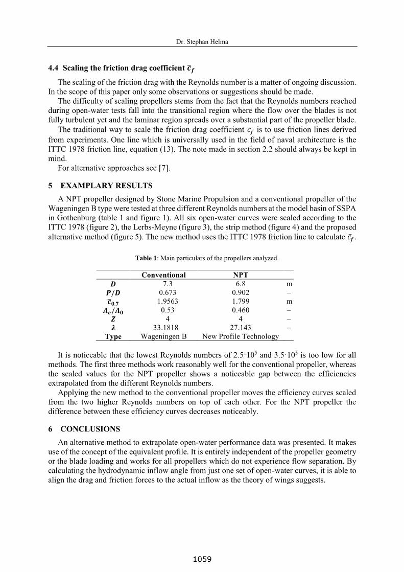
5 EXAMPLARY RESULTS A NPT propeller designed by Stone Marine Propulsion and a conventional propeller of the

Wageningen B type were tested at three different Reynolds numbers at the model basin of SSPA in Gothenburg (table 1 and figure 1). All six open-water curves were scaled according to the ITTC 1978 (figure 2), the Lerbs-Meyne (figure 3), the strip method (figure 4) and the proposed alternative method (figure 5). The new method uses the ITTC 1978 friction line to calculate 𝑐𝑐�̅�𝑓.

Table 1: Main particulars of the propellers analyzed.

Conventional NPT 𝑫𝑫 7.3 6.8 m

𝑷𝑷/𝑫𝑫 0.673 0.902 – �̅�𝒄𝟎𝟎.𝟕𝟕 1.9563 1.799 m

𝑨𝑨𝒆𝒆/𝑨𝑨𝟎𝟎 0.53 0.460 – 𝒁𝒁 4 4 – 𝝀𝝀 33.1818 27.143 –

Type Wageningen B New Profile Technology It is noticeable that the lowest Reynolds numbers of 2.5·105 and 3.5·105 is too low for all

methods. The first three methods work reasonably well for the conventional propeller, whereas the scaled values for the NPT propeller shows a noticeable gap between the efficiencies extrapolated from the different Reynolds numbers.

Applying the new method to the conventional propeller moves the efficiency curves scaled from the two higher Reynolds numbers on top of each other. For the NPT propeller the difference between these efficiency curves decreases noticeably.

6 CONCLUSIONS An alternative method to extrapolate open-water performance data was presented. It makes

use of the concept of the equivalent profile. It is entirely independent of the propeller geometry or the blade loading and works for all propellers which do not experience flow separation. By calculating the hydrodynamic inflow angle from just one set of open-water curves, it is able to align the drag and friction forces to the actual inflow as the theory of wings suggests.

1059

Dr. Stephan Helma

10

This alternative method has the potential to replace the existing methods as shown in the exemplary results.

This new method should be applied to as many performance predictions as possible and compared with the respective trials data to validate its suitability. This can only be done by a model basin which has the extensive data base to make this comparison reliable.

It was also shown that the ITTC 1978 recommendation for a minimum Reynolds number of 2·105 might be too low and it should be considered to be raised.

ACKNOWLEDGEMENTS This research was made possible due to Stone Marine Propulsion Ltd positive attitude

towards a new scaling method. A special thanks goes to Heinrich Streckwall from HSVA who kindly offered to calculate the open-water curves according to the Lerbs-Meyne- and the new strip method.

REFERENCES [1] Kuiper, G. The Wageningen Propeller Series. MARIN Publication 92-001, Wageningen,

The Netherlands (1992). [2] Meyne, K. Experimentelle und theoretische Betrachtungen zum Maßstabseffekt bei

Modellpropeller-Untersuchungen. Schiffstechnik, Vol 15 (1968). [3] Streckwall, H., Greitsch, L., Müller, J., Scharf, M. and Bugalski, T. Development of a Strip

Method Proposed to Serve as a New Standard for Propeller Performance Scaling. Ship Technology Research (2013) 60, No. 2, p. 58-60.

[4] ITTC. 1978 ITTC Performance Prediction Method. ITTC – Recommended Procedures and Guidelines, 7.5 – 02 – 03 – 01.4 (1999).

[5] Kramer, K.N. The Induced Efficiency of Optimum Propellers Having a Finite Number of Blades. NACA TM 884 (1939).

[6] Hoerner, S. Fluid Dynamic Drag: Practical Information on Aerodynamic Drag and Hydrodynamic Resistance. Hoerner Fluid Dynamics (1965).

[7] Helma, S. A Scaling Procedure for Modern Propeller Designs. A. Yücel Odabaşı Colloquium Series, 1st International Meeting - Propeller Noise & Vibration, Istanbul, Turkey, 6th – 7th November 2014.

[8] Abbott, I.H. and von Doenhoff, A.E. Theory of Wing Sections. Dover Publications, Inc, New York, USA (1959).

1060

Dr. Stephan Helma

11

Conventional Propeller NPT Propeller

Figure 1: Open-water characteristics, measured values.

Conventional Propeller NPT Propeller

Figure 2: Open-water characteristics scaled according to the ITTC 1978 method.

1061

Dr. Stephan Helma

12

Conventional Propeller NPT Propeller

Figure 3: Open-water characteristics scaled with the Lerbs-Meyne method. (Courtesy of H. Streckwall.)

Conventional Propeller NPT Propeller

Figure 4: Open-water characteristics scaled with the strip method. (Courtesy of H. Streckwall.)

1062

Dr. Stephan Helma

13

Conventional Propeller NPT Propeller

Figure 5: Open-water characteristics of the conventional propeller, scaled with the new method.

1063