Guidelines for Numerical Flow Simulation around Marine Propeller

1st International Symposium on Naval Architecture and MaritimeYTU campus, Istanbul (INT-NAM 2011) on October 24-25, 2011.

1

Guidelines for Numerical Flow Simulation around Marine Propeller

Prof. Mosaad M. A., Port Said University, Egypt, [email protected]

Prof. Mosleh M., Alexandria University Egypt [email protected]

Ass. Prof. Dr. El-Kilani H. Port Said University, Egypt [email protected]

Dr. Yehia,W. Port Said University, Egypt [email protected]

Abstract

The flow around a marine propeller is one of the most challenging hydrodynamics problems.Computational fluid dynamics (CFD) has emerged as a potential tool in recent years and haspromising applications. The goal of this paper is to provide complete guidelines for geometrycreation, boundary conditions setup, and solution parameters of the flow around rotating propeller.These guidelines are addressed to handle propeller simulation problems in order to achieve quick,more accurate solution with less computational cost. In this paper CFD results for flow around amarine propeller are presented. Computations were performed for various advance ratios followingexperimental conditions. Reynolds-Averaged Navier-Stokes (RANS) method combined with anextensive validation of two different turbulence models k– and k– was applied for the flowsimulation. The computations enable direct comparison of the reliable CFD results with theexperimental data.

Key-Words: - Propeller flow, CFD simulation, RANS

1. Introduction

The flow around the propeller is complexdue to its geometry and the combinedrotation and advancement into water. Theavailability of numerical techniques andlow cost high-speed computationalcapability has made a major impact on theanalysis of complex flows. Computationalfluid dynamics with regard to thesespecific applications is still in a process ofevolution, as is evidenced from specificvalidation studies in current researchliterature.

RANS computations offer that possibility,and such viscous-flow computations startto be used in the practical ship design; buthow accurate these predictions are, and towhat extent they depend on the turbulencemodelling used, is not really known [1].Despite of the great advancement in theCFD technologies and feasibilities of theapproaches for marine propeller flows,some issues need to be addressed for morepracticable procedures. The complexity ingeometry, mesh generation and turbulencemodelling are the main obstacles. In fact a

marine propeller is a very complexgeometry, with variable section profiles,chord lengths and pitch angles, and inoperational conditions it induces rotatingflow and entails tip vortex [2].In order to verify the reliability of the CFDsimulations, the flow about a propellermodel DTMB-P4119 propeller isinvestigated, and the results are comparedwith the existing available experimentalresults.

2. Basic MethodologyNumerical studies were carried out usingcomputational fluid dynamics [FLUENTR12] to obtain the open watercharacteristics of propeller model as well asthe distribution of pressure on the bladesurface. This effort involves standardizationof the computational grid domain withproper choice of the grid size and controlvolume around the propeller underinvestigation.

The general conservative form of the Navier– Stokes equation is presented as thecontinuity equation

mailto:[email protected]





2

Continuity equation,

mii

Suxt

)( (2.1)

Where: = density, kg/m3

iu = is the velocity component in the ith

direction, m/s (i =1, 2, 3) andS m = source terms.

In case of incompressible flows the densityis considered to be constant. Since thepropeller flow has been considered assteady and incompressible, the continuityequation gets modified as,

0)( ii

ux (2.2)

The momentum equation will be,

iij

ij

i

jij

i

Fgxx

p

uux

ut

)()(

(2.3)

Where:

ijl

l

i

j

j

iij x

uxu

xu

32)]([ , ( 2.4)

ij = is the Reynolds stress tensorp = static pressure, N/m2

gi = gravitational acceleration in the ith

direction , m/s2

Fi = external body forces in the ithdirection and, N

ij is the Kronecker delta and is equal tounity when i=j; and zero when i j.The Reynolds-Averaged form of the abovemomentum equation including theturbulent shear stresses is given by:

jiji

i

i

i

j

j

i

j

jij

i

uuxx

p

xu

xu

xu

x

uux

ut

32

(2.5)

Where:'iu = is the instantaneous velocity

component, m/s (i = 1,2, 3).In order to characterize turbulence,additional conservation equations (orclosure equations) for k– and k– have tobe solved.

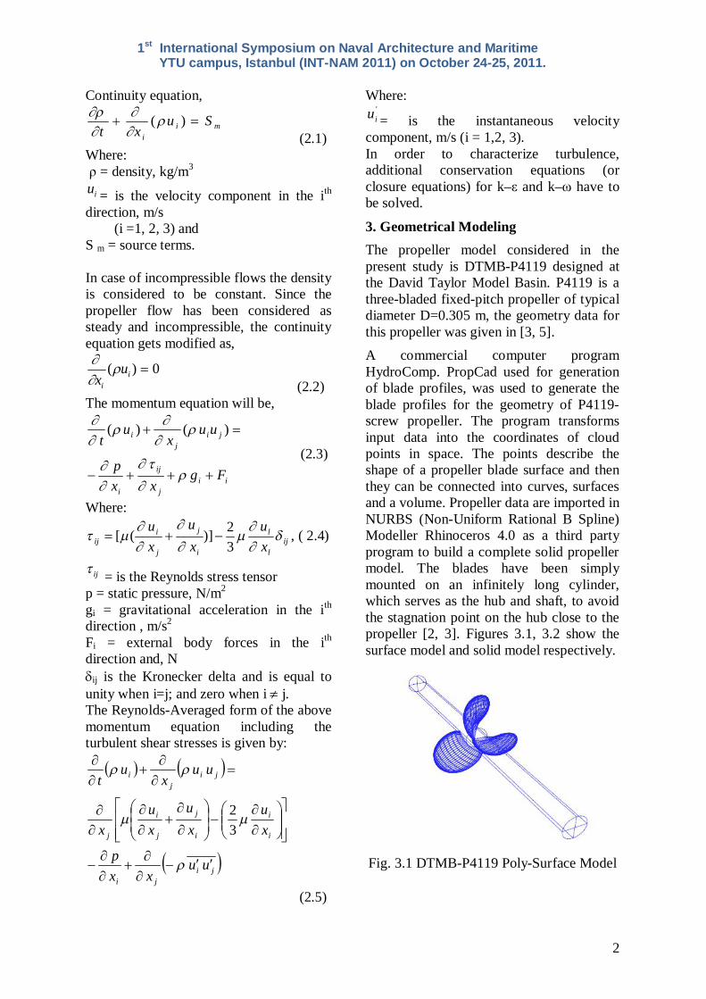
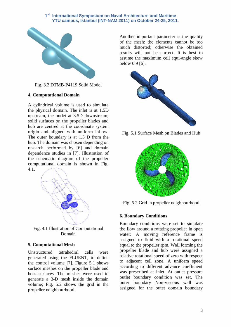
3. Geometrical ModelingThe propeller model considered in thepresent study is DTMB-P4119 designed atthe David Taylor Model Basin. P4119 is athree-bladed fixed-pitch propeller of typicaldiameter D=0.305 m, the geometry data forthis propeller was given in [3, 5].A commercial computer programHydroComp. PropCad used for generationof blade profiles, was used to generate theblade profiles for the geometry of P4119-screw propeller. The program transformsinput data into the coordinates of cloudpoints in space. The points describe theshape of a propeller blade surface and thenthey can be connected into curves, surfacesand a volume. Propeller data are imported inNURBS (Non-Uniform Rational B Spline)Modeller Rhinoceros 4.0 as a third partyprogram to build a complete solid propellermodel. The blades have been simplymounted on an infinitely long cylinder,which serves as the hub and shaft, to avoidthe stagnation point on the hub close to thepropeller [2, 3]. Figures 3.1, 3.2 show thesurface model and solid model respectively.

Fig. 3.1 DTMB-P4119 Poly-Surface Model


3

Fig. 3.2 DTMB-P4119 Solid Model

4. Computational Domain

A cylindrical volume is used to simulatethe physical domain. The inlet is at 1.5Dupstream, the outlet at 3.5D downstream;solid surfaces on the propeller blades andhub are centred at the coordinate systemorigin and aligned with uniform inflow.The outer boundary is at 1.5 D from thehub. The domain was chosen depending onresearch performed by [6] and domaindependence studies in [7]. Illustration ofthe schematic diagram of the propellercomputational domain is shown in Fig.4.1.

Fig. 4.1 Illustration of ComputationalDomain

5. Computational MeshUnstructured tetrahedral cells weregenerated using the FLUENT, to definethe control volume [7]. Figure 5.1 showssurface meshes on the propeller blade andboss surfaces. The meshes were used togenerate a 3-D mesh inside the domainvolume; Fig. 5.2 shows the grid in thepropeller neighbourhood.

Another important parameter is the qualityof the mesh: the elements cannot be toomuch distorted; otherwise the obtainedresults will not be correct. It is best toassume the maximum cell equi-angle skewbelow 0.9 [6].

Fig. 5.1 Surface Mesh on Blades and Hub

Fig. 5.2 Grid in propeller neighbourhood

6. Boundary ConditionsBoundary conditions were set to simulatethe flow around a rotating propeller in openwater: A moving reference frame isassigned to fluid with a rotational speedequal to the propeller rpm. Wall forming thepropeller blade and hub were assigned arelative rotational speed of zero with respectto adjacent cell zone. A uniform speedaccording to different advance coefficientwas prescribed at inlet. At outlet pressureoutlet boundary condition was set. Theouter boundary Non-viscous wall wasassigned for the outer domain boundary


4

with relative rotational speed of zero withrespect to adjacent cell zone [8].

7. Solver Parameters SettingThe computation conditions were based onthe research done by Jessup [4] since theexperimental results had been taken fromit. The rotational speed was set at 600 rpm.The advance coefficient was changed bychanging the velocity of inflow. Thecomputations were performed using twodifferent turbulence models k– and k–The rotational motion of the propeller wasmodelled by immobilizing the latter androtating the calculation domain in theopposite direction this gives exactly thesame results as if the propeller wererotating [6]. Computations for oneoperation point took about 24–48 hr.During this time the program computedabout 2000–3000 iterations. Solverparameter settings for the propeller openwater simulations including physicalconstants are shown in Table 7.1.

Table 7.1: Solver Parameters

8. Comparison of ResultsThe open water calculation was carried outat the same running conditions as used inthe experimental set up at [4] the calculationwas carried out for advance coefficients inthe range from 0.5 to 1.1, similar to theexperiment. The pressure field on the bladesshows low pressure on the suction side; theback of the propeller and high pressure onthe pressure side; the face of the propeller.Figures 8.1, 8.2 show the pressuredistribution on the both suction and pressuresides respectively for the tested propeller atadvance coefficient of 0.5.

Fig. 8.1 Pressure Distribution on suctionside

Fig. 8.2 Pressure Distribution on pressure

The study of the flow field shows that thepropeller accelerates the flow over theblades and introduces swirl in the flowdownstream of the propeller, as expected.

Parameter Setting

Solver 3D Segregated, Steady,Implicit

Velocity formulation Relative to adjacent cellzone

Viscous model Standard k- , k-Turbulent model

Water density 998.2kg/m3

Gradient discretization Green-Gauss CellBased

Pressure discretization Body Force WeightedMomentumdiscretization First Order Upwind

Turbulent kinetic energydiscretization First Order Upwind

Turbulence dissipationrate First Order Upwind

Pressure-velocitycoupling SIMPLE

Blade surface boundarycondition Wall (no slip)

Outer surface boundarycondition Wall (allows slip)

Water inlet boundarycondition

Velocity Inlet : Inflowat advance speed

Outflow boundarycondition Pressure outlet


5

0.4 0.5 0.6 0.7 0.8 0.9 1 1.1 1.2 1.30

0.1

0.2

0.3

0.4

0.5

0.6

0.7

0.8

J

KT, 1

0KQ

, Eta

KT Exp10KQ ExpEta ExpKT k-10KQ k-KT k-10KQ k-Eta k-Eta k-

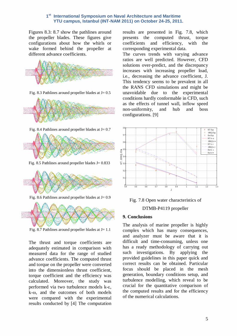
Figures 8.3: 8.7 show the pathlines aroundthe propeller blades. These figures giveconfigurations about how the whirls orwake formed behind the propeller atdifferent advance coefficients.

Fig. 8.3 Pathlines around propeller blades at J= 0.5


Fig. 8.5 Pathlines around propeller blades J= 0.833



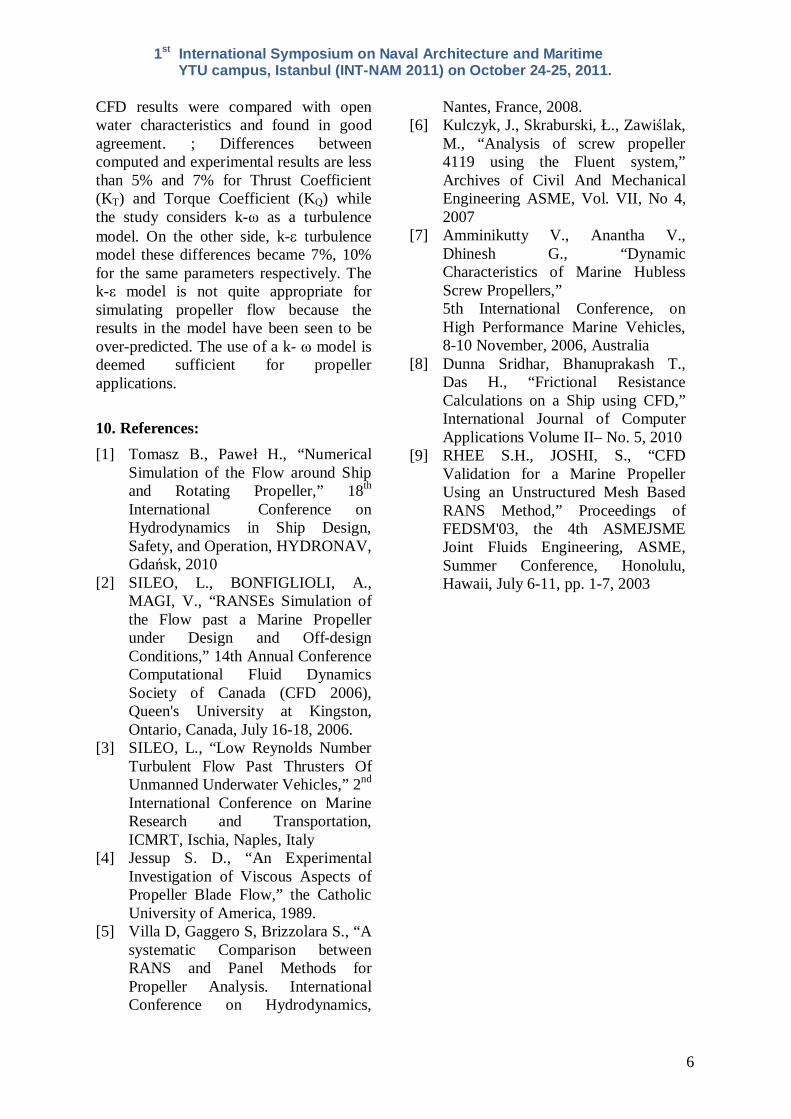
The thrust and torque coefficients areadequately estimated in comparison withmeasured data for the range of studiedadvance coefficients. The computed thrustand torque on the propeller were convertedinto the dimensionless thrust coefficient,torque coefficient and the efficiency wascalculated. Moreover, the study wasperformed via two turbulence models k- ,k- , and the outcomes of both modelswere compared with the experimentalresults conducted by [4] The computation

results are presented in Fig. 7.8, whichpresents the computed thrust, torquecoefficients and efficiency, with thecorresponding experimental data.The curves trends with varying advanceratios are well predicted. However, CFDsolutions over-predict, and the discrepancyincreases with increasing propeller load,i.e., decreasing the advance coefficient, J.This tendency seems to be prevalent in allthe RANS CFD simulations and might beunavoidable due to the experimentalconditions hardly conformable in CFD, suchas the effects of tunnel wall, inflow speednon-uniformity, and hub and bossconfigurations. [9]

Fig. 7.8 Open water characteristics of

DTMB-P4119 propeller

9. Conclusions

The analysis of marine propeller is highlycomplex which has many consequences,and analyzer must be aware that it isdifficult and time-consuming, unless onehas a ready methodology of carrying outsuch investigations. By applying theprovided guidelines in this paper quick andcorrect results can be obtained. Particularfocus should be placed in the meshgeneration, boundary conditions setup, andturbulence modelling, which reveal to becrucial for the quantitative comparison ofthe computed results and for the efficiencyof the numerical calculations.


6

CFD results were compared with openwater characteristics and found in goodagreement. ; Differences betweencomputed and experimental results are lessthan 5% and 7% for Thrust Coefficient(KT) and Torque Coefficient (KQ) whilethe study considers k- as a turbulencemodel. On the other side, k- turbulencemodel these differences became 7%, 10%for the same parameters respectively. Thek- model is not quite appropriate forsimulating propeller flow because theresults in the model have been seen to beover-predicted. The use of a k- model isdeemed sufficient for propellerapplications.

10. References:[1] Tomasz B., Pawe H., “Numerical

Simulation of the Flow around Shipand Rotating Propeller,” 18th

International Conference onHydrodynamics in Ship Design,Safety, and Operation, HYDRONAV,Gda sk, 2010

[2] SILEO, L., BONFIGLIOLI, A.,MAGI, V., “RANSEs Simulation ofthe Flow past a Marine Propellerunder Design and Off-designConditions,” 14th Annual ConferenceComputational Fluid DynamicsSociety of Canada (CFD 2006),Queen's University at Kingston,Ontario, Canada, July 16-18, 2006.

[3] SILEO, L., “Low Reynolds NumberTurbulent Flow Past Thrusters OfUnmanned Underwater Vehicles,” 2nd

International Conference on MarineResearch and Transportation,ICMRT, Ischia, Naples, Italy

[4] Jessup S. D., “An ExperimentalInvestigation of Viscous Aspects ofPropeller Blade Flow,” the CatholicUniversity of America, 1989.

[5] Villa D, Gaggero S, Brizzolara S., “Asystematic Comparison betweenRANS and Panel Methods forPropeller Analysis. InternationalConference on Hydrodynamics,

Nantes, France, 2008.[6] Kulczyk, J., Skraburski, ., Zawi lak,

M., “Analysis of screw propeller4119 using the Fluent system,”Archives of Civil And MechanicalEngineering ASME, Vol. VII, No 4,2007

[7] Amminikutty V., Anantha V.,Dhinesh G., “DynamicCharacteristics of Marine HublessScrew Propellers,”5th International Conference, onHigh Performance Marine Vehicles,8-10 November, 2006, Australia

[8] Dunna Sridhar, Bhanuprakash T.,Das H., “Frictional ResistanceCalculations on a Ship using CFD,”International Journal of ComputerApplications Volume II– No. 5, 2010

[9] RHEE S.H., JOSHI, S., “CFDValidation for a Marine PropellerUsing an Unstructured Mesh BasedRANS Method,” Proceedings ofFEDSM'03, the 4th ASMEJSMEJoint Fluids Engineering, ASME,Summer Conference, Honolulu,Hawaii, July 6-11, pp. 1-7, 2003

Guidelines for Numerical Flow Simulation around Marine Propeller

Documents

Transcript of Guidelines for Numerical Flow Simulation around Marine Propeller