Flow simulation for a propeller turbine with different runner blade geometries

Flow simulation for a propeller turbine with different runner blade geometries

This article has been downloaded from IOPscience. Please scroll down to see the full text article.

2012 IOP Conf. Ser.: Earth Environ. Sci. 15 032004

(http://iopscience.iop.org/1755-1315/15/3/032004)

Download details:

IP Address: 132.203.241.163

The article was downloaded on 23/12/2012 at 15:39

Please note that terms and conditions apply.

View the table of contents for this issue, or go to the journal homepage for more

Home Search Collections Journals About Contact us My IOPscience

http://iopscience.iop.org/page/terms

http://iopscience.iop.org/1755-1315/15/3

http://iopscience.iop.org/1755-1315

http://iopscience.iop.org/

http://iopscience.iop.org/search

http://iopscience.iop.org/collections

http://iopscience.iop.org/journals

http://iopscience.iop.org/page/aboutioppublishing

http://iopscience.iop.org/contact

http://iopscience.iop.org/myiopscience

Flow simulation for a propeller turbine with different runner blade geometries

T C Vu1, M Gauthier1, B Nennemann1, M Koller2 and C Deschenes 3 1Andritz Hydro Ltd., 6100 Transcanadienne, Pointe Claire, QC. H9R 1B9, Canada 2Andritz Hydro AG, Hardstrasse 319, 8021 Zürich, Switzerland 3LAMH, LavalUniversity, 1065 Avenue de la Médecine, Québec, QC.G1V 0A6, Canada.

E-mail: [email protected]

Abstract. In this paper, numerical flow investigation ofa propeller runner with 6 different blade runner geometries is carried out. The turbine efficiency prediction for this particular runner, performed for a wide range of operating conditions, is presented and compared to the result obtained with the average runner geometry. Also during the study, special attention is paid to the flow unsteadiness at runner outlet and in the draft tube cone at part load condition. The numerical results are validated against experimental data obtained from the AxialT project. The outcome of this comparison is important for future refurbishment projects with such particular differences in the runner blade geometry

1. Introduction AxialT, the first project undertaken by the Consortium on Hydraulic Machines, was focused on flow measurements in a propeller turbine model at the Laboratory of Hydraulic Machinery (LAMH). A series of detailed measurements have been performed on the runner model, to investigate the flow dynamic behavior over a wide range of operating conditions. Their selection was based on the runner efficiency hill chart measured on the LAMH main test rig (see figure 1and figure 2), on cavitation tests and characterization of the vortex rope across the efficiency chart. Nine operating points were initially chosen for investigation of the unsteady velocity and pressure fields in various sections of the AxialT model: draft tube, runner, rotor-stator interface and intake. Three different heads and seven different openings were targeted to cover partial load, best efficiency and overload conditions. A tenth operating point was used for investigation of the cavitating vortex rope at partial load. Detailed information on the measurement techniques can be found in [4]. For the project partners, the large set of steady and unsteady flow measurements in a low-head turbine model is a very valuable database to increase their knowledge of the flow phenomena in this type of turbine and to validate and improve their numerical flow simulation tools.

The AxialT turbine model has a semi-spiral casing with two intake channels, 24 stay vanes, 24 guide vanes and a 1950’s era 6-bladed Propeller runner. The draft tube has a short cone, an unsymmetrical elbow and one pier. Special attention has been paid to the geometry of the old runner model. The shapes of the model runner blades differ slightly from each other and the runner tip gapsvary from blade to blade. As the experimental results are obtained with a runner model with 6 different blade geometries, one should perform the CFD simulation with a set of meshes representing the runner with all six different blade geometries and with different runner blade gaps. Nicolle[5] and

26th IAHR Symposium on Hydraulic Machinery and Systems IOP PublishingIOP Conf. Series: Earth and Environmental Science 15 (2012) 032004 doi:10.1088/1755-1315/15/3/032004

Published under licence by IOP Publishing Ltd 1

Vu [7] have pointed out that a flow simulation using one of the individual blade profilesdo not allow to predict correctly the turbine efficiency curve but using the average runner geometry yields satisfactory results. In this paper, further investigationsare carried out with the AxialT runner geometry. The flow simulation for the propeller runner with 6 different runner blade geometries will be presented and compared with the results obtained with the average runner geometry. Also during the study, a special attention is paid to the flow unsteadiness at runner outlet and in the draft tube cone at part load condition. The outcome of this comparison is important for future refurbishment projects with such particular differences in the runner blade geometry.

Figure 1. Locations of flow measurements in the AxialT propeller turbine model.

Figure 2. Normalized efficiency hill chart of the AxialT propeller turbine mode.

2. Problem setup

2.1. AxialT runner blade geometry The AxialT runner is an old propeller runner model. It was re-engineered by IREQ-Hydro Quebec and Nicolle [9] has reported that the blade shapes of the runner slightly differ from each other, mostly at the leading and trailing edge regions. Vu [6] has shown that the maximum deviation to a mean position is up to ±0.5% of the throat diameter. According to IEC code which allows a maximum of ±0.1% deviation, we could not use any geometry among the six blades to simulate accurately the AxialT turbine flow behaviour. Using our own runner blade geometry design tool, we have created a new runner blade by averaging the 6 individual blade geometries. The two runner geometries, one with 6 different blade profiles and the other with an average blade profile, are used in this study.

Beside the variation on the blade geometry, the six blades have different tip clearances with the discharge ring. The tip clearance varies from 0.03% to 0.12% of the throat diameter. We keep an average blade tip clearance of 0.074% of the throat diameter for all flow simulations.

2.2. Mesh generation and computational flow domain Ideally, the computational flow domain for the CFD simulation of a hydraulic turbine should comprise the entire turbine assembly. However, we divide the steady-state simulations into two flow domains: a first flow domain comprised of the casing and the stay vanes, and a second flow domain comprised of the guide vane, runner and draft tube. As mentioned in [5] and [6], a reduced computation domain consisting of guide vanes, runner and the draft tube is adequate forthe turbine efficiency prediction. This approach has the advantage of requiring only a single simulation to determine the head loss of the casing and stay vane assembly at a given operating condition. For subsequent operating conditions, the head loss of the casing and stay vane assembly can be estimatedby assuming that the head loss is proportional to the square of the flow rate.

As shown in figure 3.a, for steady state flow simulation using mixing plane interfaces, the flow domain requires only one guide vane flow passage, one runner blade flow passage and the draft tube. But in order to perform flow simulation for the runner having 6 different blade profiles, 6 blade flow


2

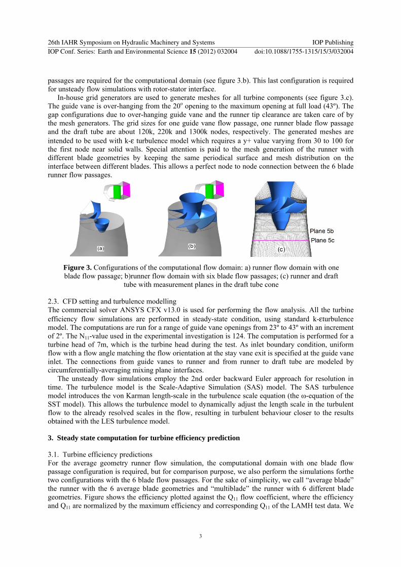
passages are required for the computational domain (see figure 3.b). This last configuration is required for unsteady flow simulations with rotor-stator interface.

In-house grid generators are used to generate meshes for all turbine components (see figure 3.c). The guide vane is over-hanging from the 20o opening to the maximum opening at full load (43º). The gap configurations due to over-hanging guide vane and the runner tip clearance are taken care of by the mesh generators. The grid sizes for one guide vane flow passage, one runner blade flow passage and the draft tube are about 120k, 220k and 1300k nodes, respectively. The generated meshes are intended to be used with k-ε turbulence model which requires a y+ value varying from 30 to 100 for the first node near solid walls. Special attention is paid to the mesh generation of the runner with different blade geometries by keeping the same periodical surface and mesh distribution on the interface between different blades. This allows a perfect node to node connection between the 6 blade runner flow passages.

Figure 3. Configurations of the computational flow domain: a) runner flow domain with one blade flow passage; b)runner flow domain with six blade flow passages; (c) runner and draft

tube with measurement planes in the draft tube cone

2.3. CFD setting and turbulence modelling The commercial solver ANSYS CFX v13.0 is used for performing the flow analysis. All the turbine efficiency flow simulations are performed in steady-state condition, using standard k-εturbulence model. The computations are run for a range of guide vane openings from 23º to 43º with an increment of 2º. The N11-value used in the experimental investigation is 124. The computation is performed for a turbine head of 7m, which is the turbine head during the test. As inlet boundary condition, uniform flow with a flow angle matching the flow orientation at the stay vane exit is specified at the guide vane inlet. The connections from guide vanes to runner and from runner to draft tube are modeled by circumferentially-averaging mixing plane interfaces.

The unsteady flow simulations employ the 2nd order backward Euler approach for resolution in time. The turbulence model is the Scale-Adaptive Simulation (SAS) model. The SAS turbulence model introduces the von Karman length-scale in the turbulence scale equation (the ω-equation of the SST model). This allows the turbulence model to dynamically adjust the length scale in the turbulent flow to the already resolved scales in the flow, resulting in turbulent behaviour closer to the results obtained with the LES turbulence model.

3. Steady state computation for turbine efficiency prediction

3.1. Turbine efficiency predictions For the average geometry runner flow simulation, the computational domain with one blade flow passage configuration is required, but for comparison purpose, we also perform the simulations forthe two configurations with the 6 blade flow passages. For the sake of simplicity, we call “average blade” the runner with the 6 average blade geometries and “multiblade” the runner with 6 different blade geometries. Figure shows the efficiency plotted against the Q11 flow coefficient, where the efficiency and Q11 are normalized by the maximum efficiency and corresponding Q11 of the LAMH test data. We


3

can see that the numerical predictions match very well with the lab data in terms of efficiency level and position of the best efficiency point. Figure 5 shows the component losses plotted against the Q11 flow coefficient, where the component losses are normalized by the sum of the losses at the best efficiency point in the LAMH test data.

Figure 4. Normalized AxialT turbine efficiency vs. normalized Q11.

Figure 5. Normalized AxialT turbine component losses vs. normalized Q11.

As expected, the results obtained for the average blade with two flow domain configurations, single blade flow and 6 blade flow passages, are almost identical. As observed in figure 5, the slight differences seen in the runner efficiency is due only to the different draft tube losses because the runner losses obtained for the two average blade configurations are identical. The numerical flow simulation shows that the multiblade runner is less efficient than the average blade runner for the whole range of operating conditions. As seen in figure 5, the head loss of the multiblade runner is consistently higher than the average blade runner while the draft tube head loss from the multiblade runner assembly is higher at off-design conditions and is equivalent with the average blade assembly around the best efficiency point.It seems logical to find that the multiblade runner is slightly less efficient than the average blade runner due to a non-uniformity of the flow in the trailing edge vicinity of the multibladerunner.

3.2. Velocity profiles in the draft tube cone In order to better understand the effect of the runner geometry on the draft tube flow, we investigate the axial and tangential velocity profiles in the draft tube cone. The CFD results are compared to velocity profiles extracted from the phase-averaged 2D-LDV velocity measurements performed by the LAMH. The measurements were performed at three elevations in the draft tube cone (numbered planes 5a, 5b and 5c), at three possible penetration orientations (33.5º, 93.5º and 153.5º). We only include the velocity profiles for the 93.5º axis on planes 5b and 5c (see figure 3b), but these profiles are representative of the other axes as well. We set user monitors in the CFD simulations at the same position as the LDV measurements. During the post-processing, the CFD velocity profiles are created by averaging the values of the user monitors over a range of iterations. In this manner, we can get averaged velocity profiles even for cases with oscillating values for the monitors.

In the velocity profile graphs (see figure 6 and figure 7), the phase-averaged measured velocities are plotted as points, and the standard deviation (representing all of the fluctuations, including the large scale periodic and turbulent fluctuations, as well as the measurement errors) is plotted as error bars. The velocities are normalized by the reference velocity, based on the flow and the throat diameter. Figure 6 and figure 7 show the axial and tangential velocity profiles for the part-load (OP1) and the best efficiency (OP3) conditions. In these figures, there is very little visible difference between the velocity profiles extracted from flow simulations with the 2 runner geometries. The exception is


4

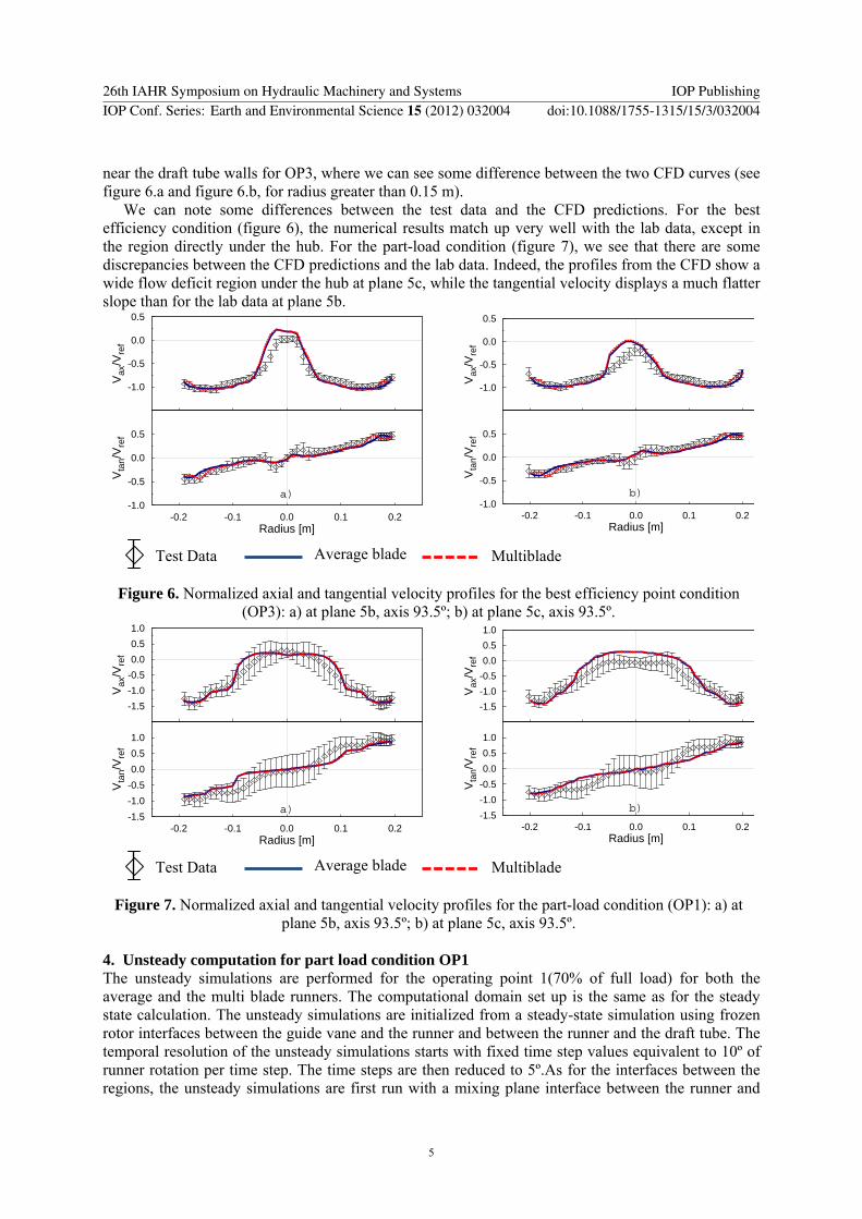
near the draft tube walls for OP3, where we can see some difference between the two CFD curves (see figure 6.a and figure 6.b, for radius greater than 0.15 m).

We can note some differences between the test data and the CFD predictions. For the best efficiency condition (figure 6), the numerical results match up very well with the lab data, except in the region directly under the hub. For the part-load condition (figure 7), we see that there are some discrepancies between the CFD predictions and the lab data. Indeed, the profiles from the CFD show a wide flow deficit region under the hub at plane 5c, while the tangential velocity displays a much flatter slope than for the lab data at plane 5b.

-1.0

-0.5

0.0

0.5

Vax

/Vre

f

-1.0

-0.5

0.0

0.5

-0.2 -0.1 0.0 0.1 0.2

Vta

n/V

ref

Radius [m]

a)

-1.0

-0.5

0.0

0.5

Vax

/Vre

f

-1.0

-0.5

0.0

0.5

-0.2 -0.1 0.0 0.1 0.2

Vta

n/V

ref

Radius [m]

b)

Figure 6. Normalized axial and tangential velocity profiles for the best efficiency point condition (OP3): a) at plane 5b, axis 93.5º; b) at plane 5c, axis 93.5º.

-1.5

-1.0

-0.5

0.0

0.5

1.0

Vax

/Vre

f

-1.5

-1.0

-0.5

0.0

0.5

1.0

-0.2 -0.1 0.0 0.1 0.2

Vta

n/V

ref

Radius [m]

a)

-1.5

-1.0

-0.5

0.0

0.5

1.0

Vax

/Vre

f

-1.5

-1.0

-0.5

0.0

0.5

1.0

-0.2 -0.1 0.0 0.1 0.2

Vta

n/V

ref

Radius [m]

b)

Figure 7. Normalized axial and tangential velocity profiles for the part-load condition (OP1): a) at plane 5b, axis 93.5º; b) at plane 5c, axis 93.5º.

4. Unsteady computation for part load condition OP1 The unsteady simulations are performed for the operating point 1(70% of full load) for both the average and the multi blade runners. The computational domain set up is the same as for the steady state calculation. The unsteady simulations are initialized from a steady-state simulation using frozen rotor interfaces between the guide vane and the runner and between the runner and the draft tube. The temporal resolution of the unsteady simulations starts with fixed time step values equivalent to 10º of runner rotation per time step. The time steps are then reduced to 5º.As for the interfaces between the regions, the unsteady simulations are first run with a mixing plane interface between the runner and

MultibladeAverage blade Test Data



5

the draft tube, followed by a transient rotor-stator. Since only one guide vane flow passage is present in the flow domain, we keep a mixing plane interface between the guide vane and the runner for all the simulations.

4.1. Static pressure in the draft tube cone The results from the unsteady CFD simulations are compared to experimental data measured by means of an unsteady pressure probe in the draft tube cone. Since we know the positions where the unsteady pressure probe data is extracted, it is possible to place user monitors to track the static pressure at the same positions in the CFD simulation. The unsteady pressure probe measurements were performed on two series of 41 points each, on plane 5c, along axes angled at 33.5º and 93.5º from the downstream axis. To simplify the comparison, we chose only two points on the 33.5º measurement axis: one point near the outer wall (point 1) and one point about halfway between the center and the wall (point 21). Figure 8 shows the positions of the two selected measurement locations in the draft tube cone.

The static pressure from the CFD simulations and from the unsteady pressure probe is plotted in figure 9 for point 1 on the 33.5º axis and figure 10 for point 21 on the 33.5º axis.We can see in both figures that the numerical results and the test data match up very well: they all share about the same amplitudes and principal frequencies. All three signals oscillate between -5 kPa and +5 kPa at point 1 on the 33.5º axis and between -25 kPa and 0 kPa at point 21 on the 33.5º axis.As for the principal frequencies, corresponding to the rope rotation frequency in the draft tube cone, they can be evaluated by counting the peaks in each signal with:

roperope

1nrope T

1f;

1n

ttT =

−−

= (1)

where Trope is the rope period, t1 and tn are the positions of the first and the nth period identified in each signal.

Figure 8. Selected unsteady measurement locations in the draft tube cone.

-25

-20

-15

-10

-5

0

5

10

0 0.5 1 1.5 2

Sta

tic P

ress

ure

[kP

a]

Time [s]

Average Blade Multiblade

Unsteady Pressure Probe

Figure 9. Static pressure in the draft tube for the average blade geometry runner at axis 1, point 1

-25

-20

-15

-10

-5

0

5

10

0 0.5 1 1.5 2

Sta

tic P

ress

ure

[kP

a]

Time [s]

Average Blade Multiblade

Unsteady Pressure Probe

Figure 10. Static pressure in the draft tube for the average blade geometry runner at axis 1, point 21.


6

Table 1 contains the estimated rope frequencies for the CFD simulations, as well as the rope frequency estimated from the unsteady pressure probe data, relative to the runner speed. We can see that rope frequency predictions match up very well for all three cases for both locations where the pressure signal was studied, with the largest relative error less than 4%.

Table 1. Estimated rope frequency relative to the runner speed from the unsteady pressure probe data and the CFD simulations.

Location CFD – average blade CFD- multiblade Unsteady pressure probe

33.5º axis, point 1 0.233 0.231 0.230

33.5º axis, point 21 0.233 0.232 0.225

4.2. Velocity profiles in the draft tube cone Figure 11 show the axial and tangential velocity profiles for the part-load (OP1) from the unsteady simulations. The velocity monitors were averaged over one period of the draft tube rope rotation, which is equivalent to about 25.8 blade passages. Much like the steady-state velocity profiles described in section 3.2. we see that there is little difference between the velocity profiles extracted from numerical results with both runner geometries. Also, we notice that it is near the walls that the CFD simulations for the two runner geometries predict slightly different velocity curves.

The CFD velocity profiles show some marked differences relative to the lab data and the steady-state numerical results. In particular, the unsteady CFD does not predict the flow deficit visible in the test data at the plane 5b (see figure 11.a) nor does it reproduce the wide flow deficit seen at plane 5c for the steady-state CFD (see figue 11.b and figure 7.b). Also, the tangential velocity curves extracted from the CFD simulations have a much more pronounced slope at plane 5b than for the lab data or for the steady-state CFD velocity profiles.

-1.5

-1.0

-0.5

0.0

0.5

1.0

Vax

/Vre

f

-1.5

-1.0

-0.5

0.0

0.5

1.0

-0.2 -0.1 0.0 0.1 0.2

Vta

n/V

ref

Radius [m]

a)

-1.5

-1.0

-0.5

0.0

0.5

1.0

Vax

/Vre

f

-1.5

-1.0

-0.5

0.0

0.5

1.0

-0.2 -0.1 0.0 0.1 0.2

Vta

n/V

ref

Radius [m]

b)

Figure 11. Normalized axial and tangential velocity profiles for the part-load condition (OP1).: a) at plane 5b, axis 93.5º; b) at plane 5c, axis 93.5º.Thick lines represent the average velocity; thin lines

represent the average ± 1 standard deviation.

5. Conclusions In this paper, numerical flow investigation of a propeller runner with 6 different blade runner geometries is carried out. The turbine efficiency prediction for this particular runner, performed for a wide range of operating condition, is presented and compared to the numerical result obtained with the average runner geometry. Both runner geometries have similar flow behaviour in steady and unsteady flow simulations. The predicted turbine efficiency curves agree very well with the experimental data in terms of the efficiency level and the position of the best efficiency point. The average runner



7

geometry is slightly more efficient possibly due to a non-uniform flow at the exit of the multiblade runner.

With the unsteady flow simulation at part load condition, similar results are obtained with the two runner geometries. The rope frequency and the pressure amplitude fluctuation match very well with the unsteady pressure measurement in the draft tube cone. In conclusion we can say that the use of average runner blade geometry to represent an old runner with slightly different blade profile geometries is satisfactory for flow simulation.

Acknowledgments The in-house mesh generators used for the study were developed by project Gmath, a joint R&D project between ÉcolePolytechnique de Montréal and Andritz Hydro Ltd. The authors would like to thank the participants on the Consortium on Hydraulic Machines for their support and contribution to this research project: Alstom Hydro Canada Inc., Andritz Hydro Ldt., Edelca, Hydro-Quebec, Laval University, NRCan, Voith Hydro Inc. Our gratitude goes as well to the Canadian Natural Sciences and Engineering Research Council who provided funding for this research.

References [1] Deschênes C, Ciocan G D, De Henau V, Flemming F, Huang J, Koller M, ArlozaF N, Page M,

Qian R and Vu T C 2010 General overview of the AxialTproject: a partnership for low head turbine developments IOP Conf. Ser.: Earth Environ. Sci.12 012043

[2] Gouin P, Deschênes C, Iliescu M andCiocan G D 2009 Experimental Investigation of Draft Tube Flow of an Axial Turbine by Laser Doppler Velocimetry 3rd IAHR Int. Meeting of the Workgroup on Cavitation and Dynamic Problems in Hydraulic Machinery and Systems(Brno)

[3] Duquesne P, Iliescu M, Fraser R, Deschênes C and Ciocan G D 2010 Monitoring of velocity and pressure fields within an axial turbine IOP Conf. Ser.: Earth Environ. Sci.12 012042

[4] Houde S, Iliescu M S, Fraser R, Lemay S, Ciocan G D and Deschênes C 2011, Experimental and Numerical Analysis of The Cavitating Part Load Vortex Dynamics of Low-Head Hydraulic Turbines Proc. of ASME-JSME-KSME Joint Fluids Engineering Conf. AJK2011-FED (Hamamatsu)

[5] Nicolle J, Labbé P, Gauthier G and Lussier M 2010 Impact of blade geometry differences from CFD performance analysis of existing turbines, 25th IAHR Symp. on Hydraulic Machinery and Systems (Timisoara)

[6] Vu T C, Koller M, Gauthier M and Deschênes C 2010 Flow simulation and efficiency hill chart prediction for a Propeller turbine IOP Conf. Ser.: Earth Environ. Sci.12 012040

[7] Vu T C, Koller M, Gauthier M and Deschênes C 2012 Efficiency computation and unsteady flow simulation for a Propeller turbine at design and off-design operating points Hydrovision Int. (Louisville)


8

Flow simulation for a propeller turbine with different runner blade geometries

Documents

Transcript of Flow simulation for a propeller turbine with different runner blade geometries