
Analytical, numerical, and experimental investigations of ...
Upload
khangminh22Category
view
2download
0
HAL Id: hal-00699499https://hal.archives-ouvertes.fr/hal-00699499
Submitted on 18 Jan 2022
HAL is a multi-disciplinary open accessarchive for the deposit and dissemination of sci-entific research documents, whether they are pub-lished or not. The documents may come fromteaching and research institutions in France orabroad, or from public or private research centers.
L’archive ouverte pluridisciplinaire HAL, estdestinée au dépôt et à la diffusion de documentsscientifiques de niveau recherche, publiés ou non,émanant des établissements d’enseignement et derecherche français ou étrangers, des laboratoirespublics ou privés.
Distributed under a Creative Commons Attribution - NonCommercial| 4.0 InternationalLicense
Experimental and numerical investigations of the flowaround an oar blade
Alban Leroyer, Sophie Barré, Jean-Michel Kobus, Michel Visonneau
To cite this version:Alban Leroyer, Sophie Barré, Jean-Michel Kobus, Michel Visonneau. Experimental and numericalinvestigations of the flow around an oar blade. Journal of Marine Science and Technology, SpringerVerlag (Germany), 2008, 13 (1), pp.1-15. 10.1007/s00773-007-0256-7. hal-00699499
A. Leroyer (*) · M. Visonneau
Laboratoire de Mécanique des Fluides, Ecole Centrale de
Nantes, B.P. 92101, 1 rue de la Noë, 44321 Nantes, France
e-mail: [email protected]
S. Barré
Ecole Nationale de Voile, Quiberon, France
S. Barré · J.-M. Kobus
Laboratoire de Mécanique des Fluides, Equipe Hydrodynamique,
Navale et Génie Océanique, Ecole Centrale de Nantes, Nantes,
France
Experimental and numerical investigations of the fl ow around an oar blade
Alban Leroyer · Sophie Barré · Jean-Michel Kobus
Michel Visonneau
framework is presented and the Navier–Stokes solver
and methods for handling multifl uid fl ows and moving
bodies are described. Lastly, numerical results are
compared with experimental data, highlighting an
encouraging agreement and proving the relevance and
the complementarity of both approaches.
Key words Rowing · Oar blade · Free-surface fl ow ·
Navier–Stokes solver
1 Introduction
Fluid mechanics is a scientifi c fi eld that plays a key role
in nautical sports, mostly in complex situations. This is
particularly true for rowing, for which fl uid fl ow knowl-
edge is required twice: once around the boat hull and
again around the oar blades. Moreover, all the phenom-
ena involved in rowing (the movement of rowers, the
forces acting on the oars, and the behaviour and resis-
tance of the hull) strongly interact. Consequently, the
only means of analysing and understanding rowing is to
use dynamic simulations. Therefore, since 1998 the Fluid
Mechanics Laboratory of Ecole Centrale de Nantes
(LMF) has developed a simulator for a complete boat–
oarsmen–oars system. This tool constitutes a means of
forging a permanent and operational synthesis of the
research and studies on rowing. The accuracy of simula-
tions evolves according to the progress in results and
validations. The relevance and the applicability of our
simulator required a thorough study of the phenomena
involved in oar propulsion. Large variations in speed
added to the heave and pitch of the boat induced by the
movement of oarsmen during the rowing stroke, make
the fl ow around rowing boats diffi cult to investigate.
Abstract This article aims at verifying the capabilities
of a Reynolds–Averaged Navier–Stokes Equations
(RANSE) solver (ISIS-CFD, developed at the Fluid
Mechanics Laboratory of Ecole Centrale de Nantes
[LMF]) to accurately compute the fl ow around an oar
blade and to deduce the forces on it and other quantities
such as effi ciency. This solver is structurally capable of
computing the fl ow around any blade shape for any
movement in six degrees of freedom, both when the
blade pierces the free surface of the water and when it
does not. To attempt a fi rst validation, a computation
was performed for a simplifi ed case chosen among those
for which experimental results are available at LMF. If
results prove satisfactory for a simplifi ed blade shape
and for a movement that respects the main characteris-
tics of blade kinematics, then the solver could be used
for real oars and more realistic kinematics. First, the
experimental setup is considered, and the objectives,
methodologies, and procedures are elucidated. The
choice of the test case for numerical validation is
explained, i.e., a plane rectangular blade with a constant
immersion and a specifi ed movement deduced from
analogy with tests on propellers. Next, the numerical
1
However, the fl ow around an oar blade appears far more
complex and has been far less studied.
Most authors adopt the very simple model suggested
by Wellicome1 to evaluate the force on oar blades and
to develop considerations on optimisation of oar setting
and rowing style. This model supposes that the force is
perpendicular to the blade and proportional to the
square of the normal component of the instantaneous
absolute velocity calculated at the centre of the blade.
This quasi-static model is dimensionally consistent, but
the coeffi cient of proportionality is never precisely
specifi ed. Some computational fl uid dynamics (CFD)
studies have been carried out using Videv2 to calculate
this coeffi cient in a two-dimensional case without a
free surface, but this simplifi ed confi guration is too far
from the specifi city of fl ow around oar blades to be
helpful.
To improve the evaluation of efforts on blades induced
by such a complex fl ow, only an experimental approach
seemed to be feasible until a few years ago. To perform
such experiments, the LMF built a sophisticated device
for testing blades at reduced scale and also for testing
real scull oars in its towing tank. Nevertheless, during
the past decade, thanks to the growth of storage capacity
and computing power, CFD tools have become no
longer limited to simple physical problems and have
signifi cantly enlarged their fi eld of applications. The
in-house Reynolds–Averaged Navier–Stokes Equations
(RANSE) solver ISIS-CFD integrates new physical fea-
tures to deal with increasingly realistic applications, such
as moving bodies and complex free-surface fl ows. Thus,
it seemed to us that the time had come to compare the
results of CFD simulations with experimental results on
such a complex confi guration. As a result, initial simula-
tions have been recently performed. To explain our
approach to the problem and to comment on the results
are thus the main goals of the present article, which is
devoted to the experimental and numerical aspects of
oar blade hydrodynamics.
First, Sect. 2 describes the experimental approach, the
procedure, and the aims of such a study. The experimen-
tal confi guration chosen for comparison with the numer-
ical results is one of those tested during a testing
campaign, the aim of which was to build a model of
hydrodynamic forces on a blade as a function of the
movement in the water and the geometric characteristics.
To discuss this modelling is not the subject of this article;
nor is it intended to make any conclusions about real
rowing styles. Here, the test bench and the associated
procedures are described, so that the reader can evaluate
the degree of confi dence which can be afforded to the
experimental results. The blade chosen for the study is
the reference blade of systematic tests, that is to say, a
plane rectangular blade with a rigid shaft moving with
analytical kinematics defi ned by only two parameters.
The reasons for this selected confi guration for numerical
validation conclude Sect. 2.
In Sect. 3, the numerical methods are considered and
the main features of the RANSE solver are given. Special
attention is paid to the numerical treatment of the
moving grid in the Navier–Stokes equations. This point
needs to be addressed as soon as body motion is encoun-
tered. Next, the simulations performed for this initial
study on an oar blade are detailed in terms of meshes,
boundary conditions, law of motion. The time evolution
of the free surface is lastly described. In Sect. 4, compari-
sons between available experimental measurements and
simulations are shown. Forces and torque are consid-
ered fi rst. A comparison of experimental and numerical
evaluation of effi ciency completes the discussion. Lastly,
conclusions highlight the complementarity of both
approaches and the perspectives of such research.
2 Experimental approach
2.1 General methodology of the test campaigns
Instrumented boats are now commonly used to measure
the motions and forces acting on oar blades. Such tests
have already been performed, in particular at LMF.
They have the advantage of working directly on a real-
istic confi guration, but the complexity of in-situ mea-
surements, which involve numerous and sometimes not
precisely controlled parameters, does not allow adequate
precision and repeatability to build or validate models
of forces on blades. For example, it is technically diffi -
cult to measure the hydrodynamic force on a blade, and
the position (or velocity) of blades is not precisely known
because of oar fl exibility and variable immersion. Thus,
in-situ measurements have been preferentially used until
now for comparative analysis and for global validation
of rowing simulations. Another approach is to repro-
duce as well as possible the movements of blades in a
towing tank. This technique permits the separation of
the propulsive device (the oar) from the motor (the
oarsman) and from the boat, as it is done for propellers.
Such a system was designed at LMF3 for testing real oars
or models of blades at a reduced scale with a rigid shaft.
The system generates a simplifi ed rowing stroke but with
good control of the parameters and with accurate repro-
ducibility. In order to avoid a complex mechanism, the
blades always remain in the water. To limit the conse-
quences of this feature, it is possible to impose a move-
ment (denoted the neutral movement) calculated to
minimise the drag on the blade before the catch angle of
2
the real stroke. This technique introduces supplementary
parameters such as the neutral motion duration and the
transition phase duration (the catch). In order to perform
systematic tests, we also defi ned simplifi ed movements
with only two kinematic parameters specifi ed under effi -
ciency considerations, as described later.
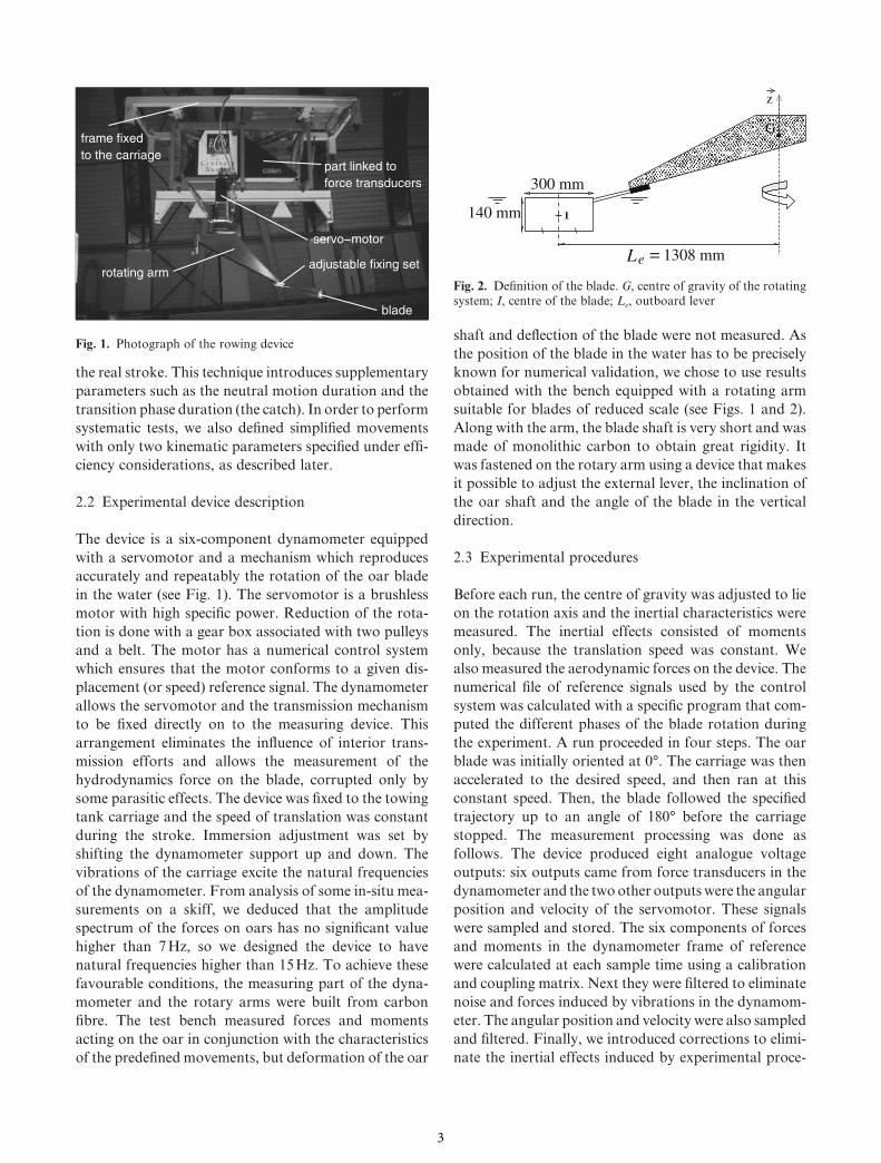
2.2 Experimental device description
The device is a six-component dynamometer equipped
with a servomotor and a mechanism which reproduces
accurately and repeatably the rotation of the oar blade
in the water (see Fig. 1). The servomotor is a brushless
motor with high specifi c power. Reduction of the rota-
tion is done with a gear box associated with two pulleys
and a belt. The motor has a numerical control system
which ensures that the motor conforms to a given dis-
placement (or speed) reference signal. The dynamometer
allows the servomotor and the transmission mechanism
to be fi xed directly on to the measuring device. This
arrangement eliminates the infl uence of interior trans-
mission efforts and allows the measurement of the
hydrodynamics force on the blade, corrupted only by
some parasitic effects. The device was fi xed to the towing
tank carriage and the speed of translation was constant
during the stroke. Immersion adjustment was set by
shifting the dynamometer support up and down. The
vibrations of the carriage excite the natural frequencies
of the dynamometer. From analysis of some in-situ mea-
surements on a skiff, we deduced that the amplitude
spectrum of the forces on oars has no signifi cant value
higher than 7 Hz, so we designed the device to have
natural frequencies higher than 15 Hz. To achieve these
favourable conditions, the measuring part of the dyna-
mometer and the rotary arms were built from carbon
fi bre. The test bench measured forces and moments
acting on the oar in conjunction with the characteristics
of the predefi ned movements, but deformation of the oar
shaft and defl ection of the blade were not measured. As
the position of the blade in the water has to be precisely
known for numerical validation, we chose to use results
obtained with the bench equipped with a rotating arm
suitable for blades of reduced scale (see Figs. 1 and 2).
Along with the arm, the blade shaft is very short and was
made of monolithic carbon to obtain great rigidity. It
was fastened on the rotary arm using a device that makes
it possible to adjust the external lever, the inclination of
the oar shaft and the angle of the blade in the vertical
direction.
2.3 Experimental procedures
Before each run, the centre of gravity was adjusted to lie
on the rotation axis and the inertial characteristics were
measured. The inertial effects consisted of moments
only, because the translation speed was constant. We
also measured the aerodynamic forces on the device. The
numerical fi le of reference signals used by the control
system was calculated with a specifi c program that com-
puted the different phases of the blade rotation during
the experiment. A run proceeded in four steps. The oar
blade was initially oriented at 0°. The carriage was then
accelerated to the desired speed, and then ran at this
constant speed. Then, the blade followed the specifi ed
trajectory up to an angle of 180° before the carriage
stopped. The measurement processing was done as
follows. The device produced eight analogue voltage
outputs: six outputs came from force transducers in the
dynamometer and the two other outputs were the angular
position and velocity of the servomotor. These signals
were sampled and stored. The six components of forces
and moments in the dynamometer frame of reference
were calculated at each sample time using a calibration
and coupling matrix. Next they were fi ltered to eliminate
noise and forces induced by vibrations in the dynamom-
eter. The angular position and velocity were also sampled
and fi ltered. Finally, we introduced corrections to elimi-
nate the inertial effects induced by experimental proce-
force transducers
part linked to to the carriage
frame fixed
adjustable fixing set
blade
servo−motor
rotating arm
Fig. 1. Photograph of the rowing device
z
300 mm
140 mm
G
1308 mm=eL
I
Fig. 2. Defi nition of the blade. G, centre of gravity of the rotating
system; I, centre of the blade; Le, outboard lever
3
dures so as to obtain only the hydrodynamic forces and
moments. The different stages are described below.
Sampling and measurement acquisition. For mea-
surements acquisition, we use an A/D converter card
controlled by an advanced program. This program
permits the defi nition of acquisition sequences and stored
them. The sampling frequency was chosen to be 500 Hz
to avoid using an anti-aliasing fi lter.
Filtering. The fi ltering method consisted of a low-
pass windowing spectrum followed by a reconstitution
of the signal by applying an inverse Fourier transform.
This technique did not induce any phase shift between
measured signals. A band of frequency between 7 and
15 Hz having very low spectral power allowed low-pass
fi ltering to be performed with good precision and with
few induced perturbations in the pass band.
Pre-processing. This procedure consisted fi rst in
ordering and storing raw data and fi ltered data, and
second in correcting data using inertial and aerodynamic
effects.
Measurement exploitation. First, the physical param-
eters used for analysis and modelling were computed,
and second, kinematic data and forces measured in the
dynamometer axis were used to calculate the forces in a
different axis (e.g., the blade axis or the relative inci-
dence of water). Finally, hydrodynamic coeffi cients, the
instantaneous driving force, the effective power, and the
instantaneous and global effi ciencies were evaluated.
2.4 Blade kinematics and effi ciency considerations
To begin with, some notations were defi ned as follows
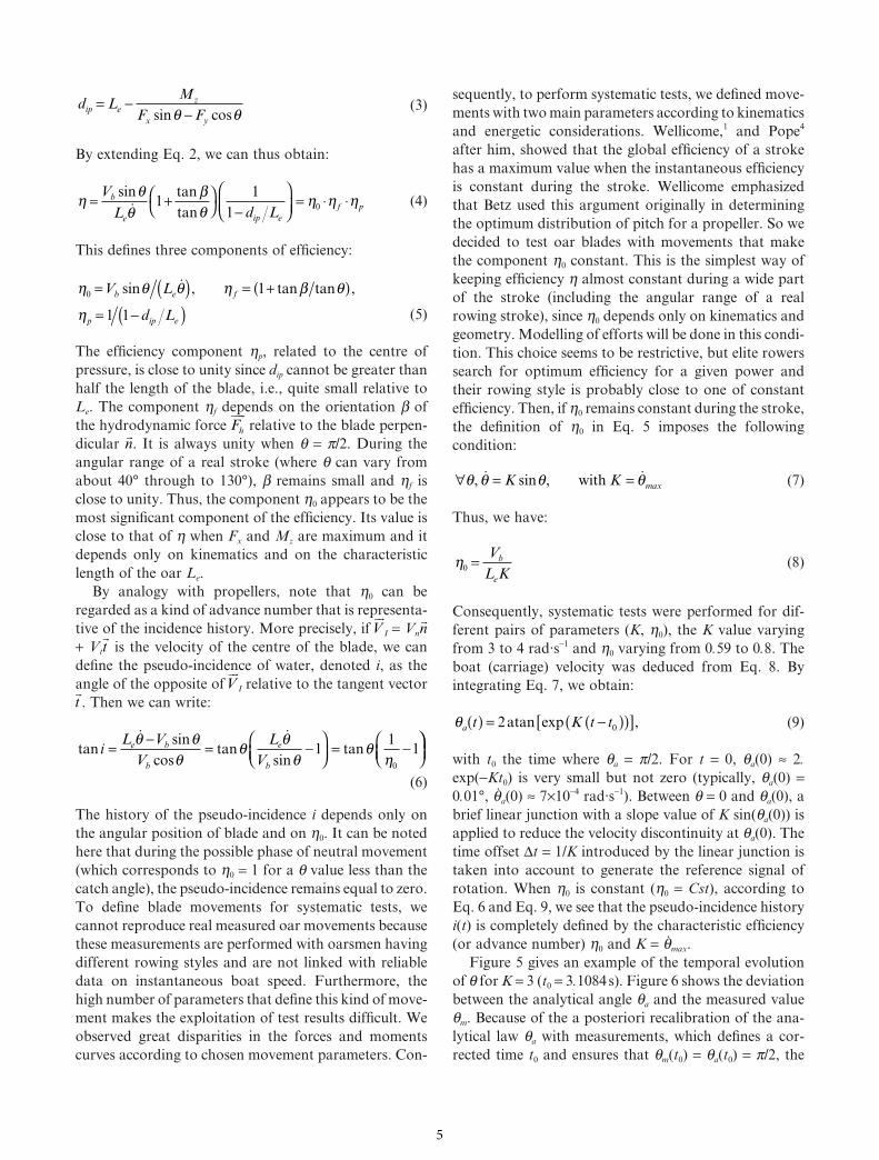
and are represented in Figs. 2–4.
Geometry and kinematics
• (xc
, yc
, zc
): frame of reference linked to the carriage
(or boat), with z upward and the motion of the car-
riage directed towards −xc
• (t , n, z): frame of reference linked to the blade, with
t
the horizontal vector tangent to the blade directed
towards the rotation axis
• Le: outboard lever (>0), i.e., the distance between the
rotation axis (O,z) and I, the centre of the blade
surface
• q = (x tc
, ): the angle between the shaft and the transla-
tional boat velocity
• b: the angle between hydrodynamic force Fh
and
n, the
vector perpendicular to the blade
• Vb = |Vb
| = −Vb
· xc
: the boat velocity (>0).
Components of horizontal hydrodynamic force Fh
and
the torque in different axes of reference (see Fig. 4)
• Fx, Fy: in the dynamometer (or boat) axis
• Ft, Fn: in the shaft axis,
• Mz: the component of the hydrodynamic torque
applied about (O, z).
The instantaneous effi ciency h is defi ned as the ratio
of the useful power to the delivered power:
ηθ
= F V
M
x b
zɺ
(1)
Let us denote the centre of the blade I, and the point
where the resultant fl uid force Fh
acts at each instant P
(see Fig. 4). Then, Eq. 1 can be formulated as:
ηθ β
β θθ β=
− ⋅ +( )⋅
+( )⋅ ⋅ ( )= +( )⋅
−
F V
OI d F
V
L
h b
ip h
b
e
ɺ
sin
cos
sin
ddip( )⋅ ( )cos,
β θɺ(2)
where dip is the algebraic distance between I and P pro-
jected on the oriented shaft axis (O, t ).
Note that Mz = −(Le − dip).Fn = (Le − dip).(Fx sin q −
Fy cos q). So, we can deduce:
yc
xc
t
θ (t)O
still water
carriageVb
blade
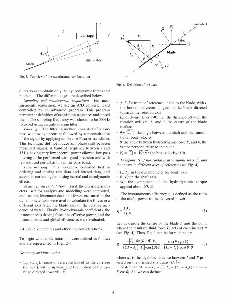
Fig. 3. Top view of the experimental confi guration
Fh
Fn
Fx
Ft
Fy
d < 0ip
tn
xc
yc
(t)θ
P
I
towards O
β
blade
Fig. 4. Defi nition of the axes
4
d LM
F Fip e
z
x y
= −−sin cosθ θ
(3)
By extending Eq. 2, we can thus obtain:
η θθ
βθ
η η η= +
−
= ⋅ ⋅V
L d L
b
e ip e
f p
sin tan
tanɺ1
1
10 (4)
This defi nes three components of effi ciency:
η θ θ η β θ
η0 1
1 1
= ( ) = +( )= −( )
V L
d L
b e f
p ip e
sin , tan tan ,ɺ
(5)
The effi ciency component hp, related to the centre of
pressure, is close to unity since dip cannot be greater than
half the length of the blade, i.e., quite small relative to
Le. The component hf depends on the orientation b of
the hydrodynamic force Fh
relative to the blade perpen-
dicular n. It is always unity when q = p/2. During the
angular range of a real stroke (where q can vary from
about 40° through to 130°), b remains small and hf is
close to unity. Thus, the component h0 appears to be the
most signifi cant component of the effi ciency. Its value is
close to that of h when Fx and Mz are maximum and it
depends only on kinematics and on the characteristic
length of the oar Le.
By analogy with propellers, note that h0 can be
regarded as a kind of advance number that is representa-
tive of the incidence history. More precisely, if V
I = Vn
n
+ Vt
t is the velocity of the centre of the blade, we can
defi ne the pseudo-incidence of water, denoted i, as the
angle of the opposite of V
I relative to the tangent vector t . Then we can write:
tansin
costan
sintani
L V
V
L
Ve b
b
e
b
= − = −
= −
ɺ ɺθ θθ
θ θθ
θη
11
10
(6)
The history of the pseudo-incidence i depends only on
the angular position of blade and on h0. It can be noted
here that during the possible phase of neutral movement
(which corresponds to h0 = 1 for a q value less than the
catch angle), the pseudo-incidence remains equal to zero.
To defi ne blade movements for systematic tests, we
cannot reproduce real measured oar movements because
these measurements are performed with oarsmen having
different rowing styles and are not linked with reliable
data on instantaneous boat speed. Furthermore, the
high number of parameters that defi ne this kind of move-
ment makes the exploitation of test results diffi cult. We
observed great disparities in the forces and moments
curves according to chosen movement parameters. Con-
sequently, to perform systematic tests, we defi ned move-
ments with two main parameters according to kinematics
and energetic considerations. Wellicome,1 and Pope4
after him, showed that the global effi ciency of a stroke
has a maximum value when the instantaneous effi ciency
is constant during the stroke. Wellicome emphasized
that Betz used this argument originally in determining
the optimum distribution of pitch for a propeller. So we
decided to test oar blades with movements that make
the component h0 constant. This is the simplest way of
keeping effi ciency h almost constant during a wide part
of the stroke (including the angular range of a real
rowing stroke), since h0 depends only on kinematics and
geometry. Modelling of efforts will be done in this condi-
tion. This choice seems to be restrictive, but elite rowers
search for optimum effi ciency for a given power and
their rowing style is probably close to one of constant
effi ciency. Then, if h0 remains constant during the stroke,
the defi nition of h0 in Eq. 5 imposes the following
condition:
∀ = =θ θ θ θ, sin ,ɺ ɺK Kwith max (7)
Thus, we have:
η0 = V
L Kb
e
(8)
Consequently, systematic tests were performed for dif-
ferent pairs of parameters (K, h0), the K value varying
from 3 to 4 rad·s−1 and h0 varying from 0.59 to 0.8. The
boat (carriage) velocity was deduced from Eq. 8. By
integrating Eq. 7, we obtain:
θa t K t t( ) = −( )( )[ ]2 0atan exp , (9)
with t0 the time where qa = p/2. For t = 0, qa(0) ≈ 2.
exp(−Kt0) is very small but not zero (typically, qa(0) =0.01°, q
.a(0) ≈ 7×10⁻⁴ rad·s−1). Between q = 0 and qa(0), a
brief linear junction with a slope value of K sin(qa(0)) is
applied to reduce the velocity discontinuity at qa(0). The
time offset ∆t = 1/K introduced by the linear junction is
taken into account to generate the reference signal of
rotation. When h0 is constant (h0 = Cst), according to
Eq. 6 and Eq. 9, we see that the pseudo-incidence history
i(t) is completely defi ned by the characteristic effi ciency
(or advance number) h0 and K = q.max.
Figure 5 gives an example of the temporal evolution
of q for K = 3 (t0 = 3.1084 s). Figure 6 shows the deviation
between the analytical angle qa and the measured value
qm. Because of the a posteriori recalibration of the ana-
lytical law qa with measurements, which defi nes a cor-
rected time t0 and ensures that qm(t0) = qa(t0) = p/2, the
5
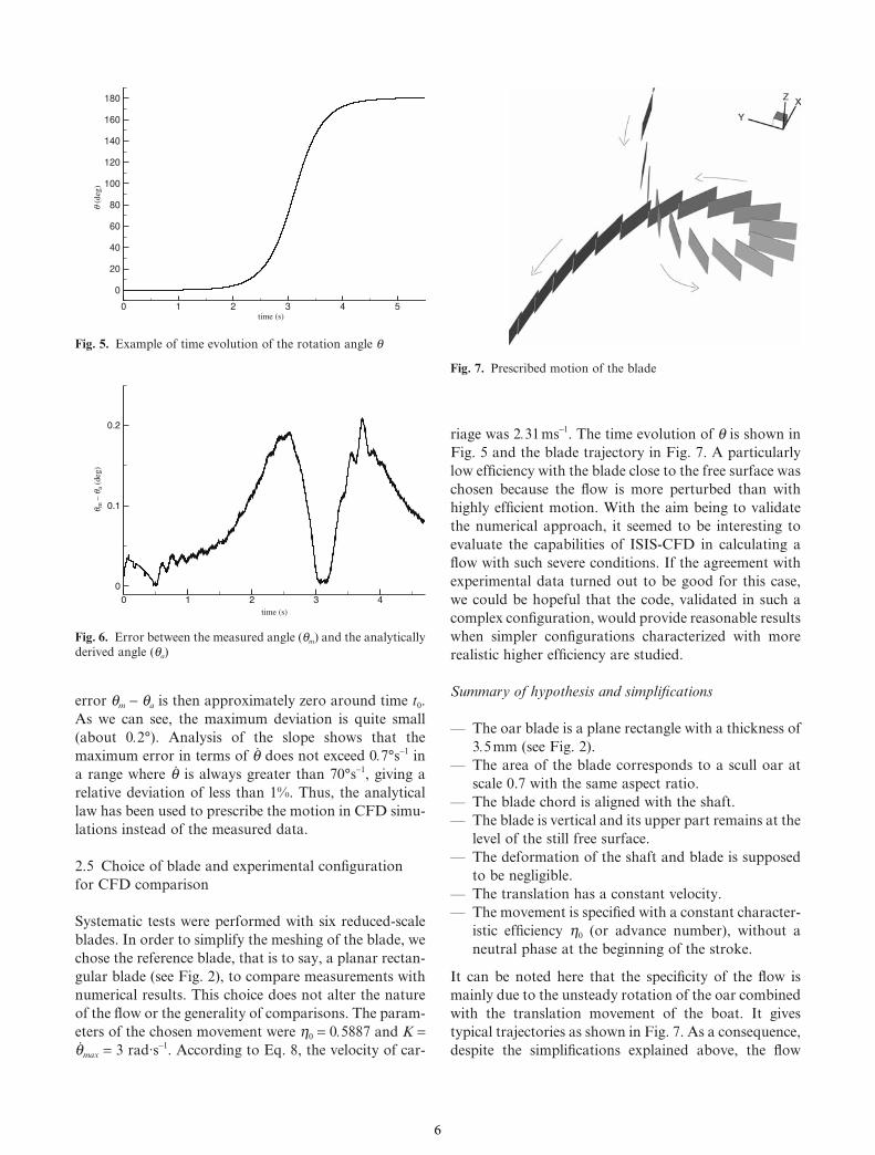
error qm − qa is then approximately zero around time t0.
As we can see, the maximum deviation is quite small
(about 0.2°). Analysis of the slope shows that the
maximum error in terms of q. does not exceed 0.7°s−1 in
a range where q. is always greater than 70°s−1, giving a
relative deviation of less than 1%. Thus, the analytical
law has been used to prescribe the motion in CFD simu-
lations instead of the measured data.
2.5 Choice of blade and experimental confi guration
for CFD comparison
Systematic tests were performed with six reduced-scale
blades. In order to simplify the meshing of the blade, we
chose the reference blade, that is to say, a planar rectan-
gular blade (see Fig. 2), to compare measurements with
numerical results. This choice does not alter the nature
of the fl ow or the generality of comparisons. The param-
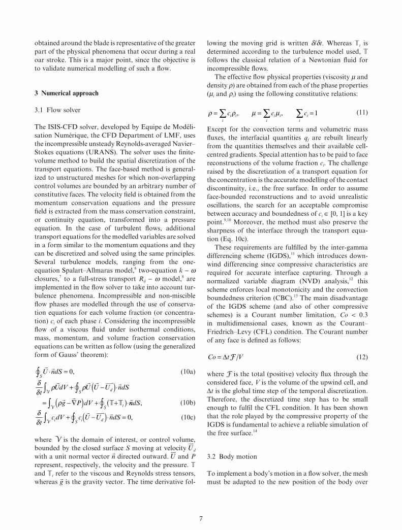
eters of the chosen movement were h0 = 0.5887 and K =q.max = 3 rad·s−1. According to Eq. 8, the velocity of car-
riage was 2.31 ms−1. The time evolution of q is shown in
Fig. 5 and the blade trajectory in Fig. 7. A particularly
low effi ciency with the blade close to the free surface was
chosen because the fl ow is more perturbed than with
highly effi cient motion. With the aim being to validate
the numerical approach, it seemed to be interesting to
evaluate the capabilities of ISIS-CFD in calculating a
fl ow with such severe conditions. If the agreement with
experimental data turned out to be good for this case,
we could be hopeful that the code, validated in such a
complex confi guration, would provide reasonable results
when simpler confi gurations characterized with more
realistic higher effi ciency are studied.
Summary of hypothesis and simplifi cations
— The oar blade is a plane rectangle with a thickness of
3.5 mm (see Fig. 2).
— The area of the blade corresponds to a scull oar at
scale 0.7 with the same aspect ratio.
— The blade chord is aligned with the shaft.
— The blade is vertical and its upper part remains at the
level of the still free surface.
— The deformation of the shaft and blade is supposed
to be negligible.
— The translation has a constant velocity.
— The movement is specifi ed with a constant character-
istic effi ciency h0 (or advance number), without a
neutral phase at the beginning of the stroke.
It can be noted here that the specifi city of the fl ow is
mainly due to the unsteady rotation of the oar combined
with the translation movement of the boat. It gives
typical trajectories as shown in Fig. 7. As a consequence,
despite the simplifi cations explained above, the fl ow
time (s)
q (
deg
)
0 1 2 3 4 5
0
20
40
60
80
100
120
140
160
180
Fig. 5. Example of time evolution of the rotation angle q
time (s)
qm
– q
a (d
eg)
0 1 2 3 4
0
0.1
0.2
Fig. 6. Error between the measured angle (qm) and the analytically
derived angle (qa)
Fig. 7. Prescribed motion of the blade
6
obtained around the blade is representative of the greater
part of the physical phenomena that occur during a real
oar stroke. This is a major point, since the objective is
to validate numerical modelling of such a fl ow.
3 Numerical approach
3.1 Flow solver
The ISIS-CFD solver, developed by Equipe de Modéli-
sation Numérique, the CFD Department of LMF, uses
the incompressible unsteady Reynolds-averaged Navier–
Stokes equations (URANS). The solver uses the fi nite-
volume method to build the spatial discretization of the
transport equations. The face-based method is general-
ized to unstructured meshes for which non-overlapping
control volumes are bounded by an arbitrary number of
constitutive faces. The velocity fi eld is obtained from the
momentum conservation equations and the pressure
fi eld is extracted from the mass conservation constraint,
or continuity equation, transformed into a pressure
equation. In the case of turbulent fl ows, additional
transport equations for the modelled variables are solved
in a form similar to the momentum equations and they
can be discretized and solved using the same principles.
Several turbulence models, ranging from the one-
equation Spalart–Allmaras model,6 two-equation k − w
closures,7 to a full-stress transport Rij − w model,8 are
implemented in the fl ow solver to take into account tur-
bulence phenomena. Incompressible and non-miscible
fl ow phases are modelled through the use of conserva-
tion equations for each volume fraction (or concentra-
tion) ci of each phase i. Considering the incompressible
fl ow of a viscous fl uid under isothermal conditions,
mass, momentum, and volume fraction conservation
equations can be written as follow (using the generalized
form of Gauss’ theorem):
U ndS⋅ =∫ 0,
S(10a)
δδ
ρ ρ
ρt
UdV U U U ndS
g P dV
d
t
V S
V S
∫ ∫∫ ∫
+ −( )⋅= − ∇( ) + +( )⋅ nndS, (10b)
δδt
c dV c U U ndSi i dV S∫ ∫+ −( )⋅ =
0, (10c)
where V is the domain of interest, or control volume,
bounded by the closed surface S moving at velocity U
d
with a unit normal vector n directed outward. U
and P
represent, respectively, the velocity and the pressure.
and t refer to the viscous and Reynolds stress tensors,
whereas g is the gravity vector. The time derivative fol-
lowing the moving grid is written d/dt. Whereas t is
determined according to the turbulence model used,
follows the classical relation of a Newtonian fl uid for
incompressible fl ows.
The effective fl ow physical properties (viscosity m and
density r) are obtained from each of the phase properties
(mi and ri) using the following constitutive relations:
ρ ρ µ µ= = =∑ ∑ ∑c c ci i
i
i i
i
i
i
, , 1 (11)
Except for the convection terms and volumetric mass
fl uxes, the interfacial quantities qf are rebuilt linearly
from the quantities themselves and their available cell-
centred gradients. Special attention has to be paid to face
reconstructions of the volume fraction ci. The challenge
raised by the discretization of a transport equation for
the concentration is the accurate modelling of the contact
discontinuity, i.e., the free surface. In order to assume
face-bounded reconstructions and to avoid unrealistic
oscillations, the search for an acceptable compromise
between accuracy and boundedness of ci ∈ [0, 1] is a key
point.9,10 Moreover, the method must also preserve the
sharpness of the interface through the transport equa-
tion (Eq. 10c).
These requirements are fulfi lled by the inter-gamma
differencing scheme (IGDS),11 which introduces down-
wind differencing since compressive characteristics are
required for accurate interface capturing. Through a
normalized variable diagram (NVD) analysis,12 this
scheme enforces local monotonicity and the convection
boundedness criterion (CBC).13 The main disadvantage
of the IGDS scheme (and also of other compressive
schemes) is a Courant number limitation, Co < 0.3
in multidimensional cases, known as the Courant–
Friedrich–Levy (CFL) condition. The Courant number
of any face is defi ned as follows:
Co t V= ∆ F (12)
where F is the total (positive) velocity fl ux through the
considered face, V is the volume of the upwind cell, and
∆t is the global time step of the temporal discretization.
Therefore, the discretized time step has to be small
enough to fulfi l the CFL condition. It has been shown
that the role played by the compressive property of the
IGDS is fundamental to achieve a reliable simulation of
the free surface.14
3.2 Body motion
To implement a body’s motion in a fl ow solver, the mesh
must be adapted to the new position of the body over
7
time. In order to keep an appropriate grid, three comple-
mentary methods have been integrated (for further
details, see Leroyer15):
— the pseudo-structure regridding procedure,
— the rigid transformation of the mesh,
— the analytical weighted regridding approach.
When the grid is moving, the so-called space conservation
law must be satisfi ed:
δδt
dV U ndSdV S∫ ∫− ⋅ = 0 (13)
The mesh mobility is then taken into account in the
equations of conservation with the grid velocity U
d, or
more precisely with the grid displacement velocity fl ux
through each face S, denoted by F SUd
. It is defi ned by:
F S
SU ddU ndS= ⋅∫
(14)
For deformation techniques (pseudo-structure analogy
and weighted regridding), this quantity is obtained by
computing the exact volumes swept by cell faces during
the time steps, which ensures that the discrete space
conservation law is exactly satisfi ed.15,16 If a rigid trans-
formation is also applied, its contribution to the dis-
placement velocity fl uxes can be exactly computed by
using the parameters of the kinematic screw Ω, U
O1 of
the rigid transformation. Indeed, for each point M geo-
metrically linked to this mesh, the velocity induced by
the rigid displacement is defi ned by:
U M U O O Md d( ) = ( ) + ⊗
1 1Ω
This property is used to generate a direct and exact cal-
culation of the grid displacement velocity fl ux through
each face S using the following:
F
F
S
S SU d d f
r
dU ndS U F S FM ndS= ⋅ = ( )⋅ + ⋅ ⊗∫ ∫
Ω
’
(15)
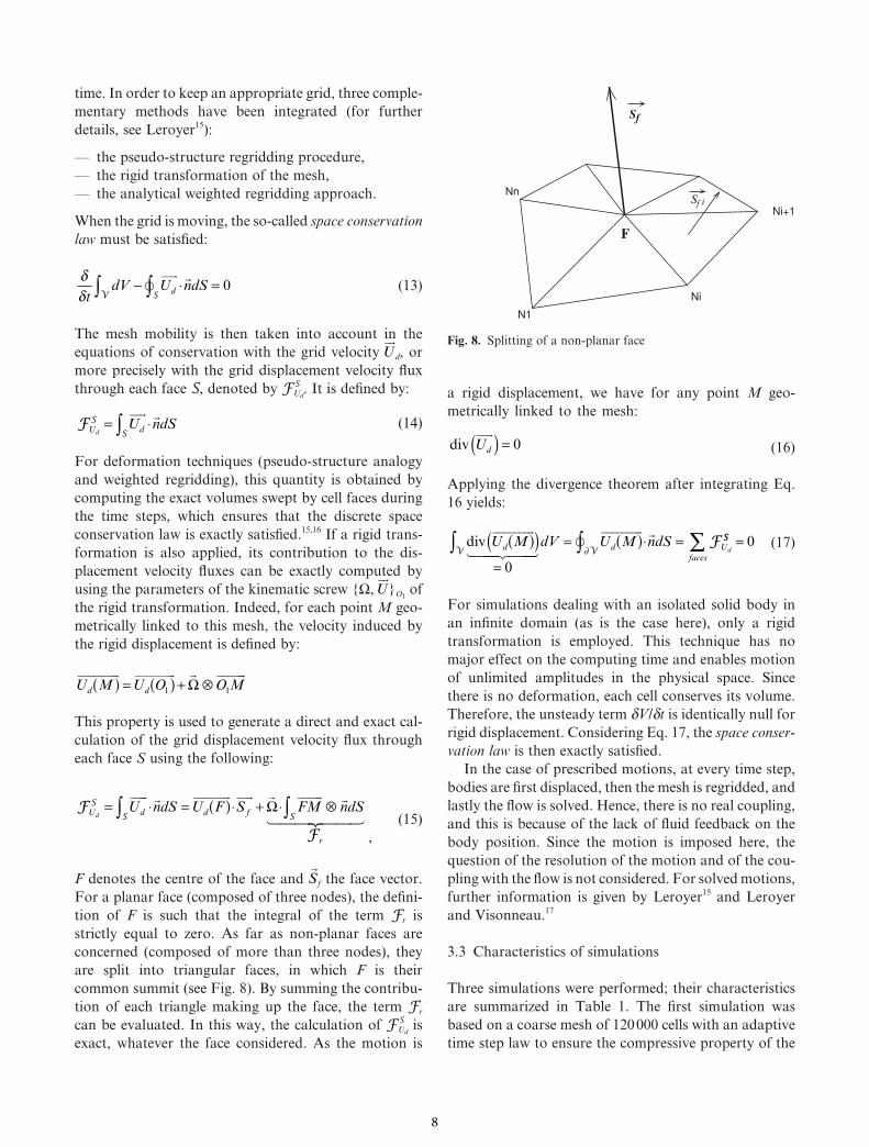
F denotes the centre of the face and Sf the face vector.
For a planar face (composed of three nodes), the defi ni-
tion of F is such that the integral of the term Fr is
strictly equal to zero. As far as non-planar faces are
concerned (composed of more than three nodes), they
are split into triangular faces, in which F is their
common summit (see Fig. 8). By summing the contribu-
tion of each triangle making up the face, the term Fr
can be evaluated. In this way, the calculation of F SUd
is
exact, whatever the face considered. As the motion is
a rigid displacement, we have for any point M geo-
metrically linked to the mesh:
div Ud
( ) = 0 (16)
Applying the divergence theorem after integrating Eq.
16 yields:
div U M dV U M ndSd d Ud( )( )
=
= ( )⋅ =∫∫
0
∂VVF SS
faces
∑ = 0 (17)
For simulations dealing with an isolated solid body in
an infi nite domain (as is the case here), only a rigid
transformation is employed. This technique has no
major effect on the computing time and enables motion
of unlimited amplitudes in the physical space. Since
there is no deformation, each cell conserves its volume.
Therefore, the unsteady term dV/dt is identically null for
rigid displacement. Considering Eq. 17, the space conser-
vation law is then exactly satisfi ed.
In the case of prescribed motions, at every time step,
bodies are fi rst displaced, then the mesh is regridded, and
lastly the fl ow is solved. Hence, there is no real coupling,
and this is because of the lack of fl uid feedback on the
body position. Since the motion is imposed here, the
question of the resolution of the motion and of the cou-
pling with the fl ow is not considered. For solved motions,
further information is given by Leroyer15 and Leroyer
and Visonneau.17
3.3 Characteristics of simulations
Three simulations were performed; their characteristics
are summarized in Table 1. The fi rst simulation was
based on a coarse mesh of 120 000 cells with an adaptive
time step law to ensure the compressive property of the
Ni+1
N1
Ni
Nn
F
Sf i
Sf
Fig. 8. Splitting of a non-planar face
8
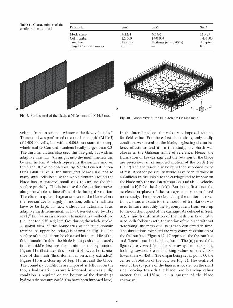
volume fraction scheme, whatever the fl ow velocities.18
The second was performed on a much fi ner grid (M14e5)
of 1 400 000 cells, but with a 0.005 s constant time step,
which lead to Courant numbers locally larger than 0.3.
The third simulation also used this fi ne grid, but with an
adaptive time law. An insight into the mesh fi neness can
be seen in Fig. 9, which represents the surface grid on
the blade. It can be noted on Fig. 9b that even if it con-
tains 1 400 000 cells, the fi nest grid M14e5 has not so
many small cells because the whole domain around the
blade has to conserve small cells to capture the free
surface precisely. This is because the free surface moves
along the whole surface of the blade during the motion.
Therefore, in quite a large area around the blade where
the free surface is largely in motion, cells of small size
have to be kept. In fact, without an automatic local
adaptive mesh refi nement, as has been detailed by Hay
et al.,18 this feature is necessary to maintain a well-defi ned
(i.e., not too diffused) interface during the whole stroke.
A global view of the boundaries of the fl uid domain
(except the upper boundary) is shown on Fig. 10. The
surface of the blade can be observed in the middle of the
fl uid domain. In fact, the blade is not positioned exactly
in the middle because the motion is not symmetric.
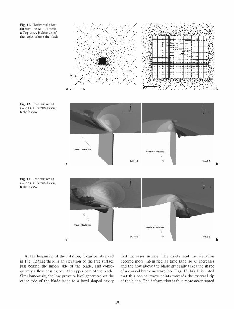
Figure 11a illustrates this point: it shows a horizontal
slice of the mesh (fl uid domain is vertically extruded).
Figure 11b is a close-up of Fig. 11a around the blade.
The boundary conditions are imposed as follows: on the
top, a hydrostatic pressure is imposed, whereas a slip
condition is required on the bottom of the domain (a
hydrostatic pressure could also have been imposed here).
In the lateral regions, the velocity is imposed with its
far-fi eld value. For these fi rst simulations, only a slip
condition was tested on the blade, neglecting the turbu-
lence effects around it. In this study, the Earth was
chosen as the Galilean frame of reference. Hence, the
translation of the carriage and the rotation of the blade
are prescribed as an imposed motion of the blade (see
Fig. 7) and the far-fi eld velocity is then supposed to be
at rest. Another possibility would have been to work in
a Galilean frame linked to the carriage and to impose on
the blade only the motion of rotation (and also a velocity
equal to V xb
for the far fi eld). But in the fi rst case, the
acceleration phase of the carriage can be reproduced
more easily. Here, before launching the motion of rota-
tion, a transient state for the motion of translation was
used to raise smoothly the Vx component from zero up
to the constant speed of the carriage. As detailed in Sect.
3.2, a rigid transformation of the mesh was favourably
used: cells follow exactly the motion of the blade without
deforming; the mesh quality is then conserved in time.
The simulations exhibited the very complex evolution of
the free surface. Figures 12–17 represent the free surface
at different times in the blade frame. The (a) parts of the
fi gures are viewed from the side away from the shaft,
looking towards t and blanking values on the
t axis
lower than −1.458 m (the origin being set at point O, the
centre of rotation of the oar, see Fig. 3). The centre of
view of the (b) parts of the fi gures is located on the shaft
side, looking towards the blade, and blanking values
greater than −1.158 m, i.e., a quarter of the blade
spanwise.
Parameter Sim1 Sim2 Sim3
Mesh name M12e4 M14e5 M14e5
Cell number 120 000 1 400 000 1 400 000
Time law Adaptive Uniform (dt = 0.005 s) Adaptive
Target Courant number 0.3 — 0.3
Table 1. Characteristics of the
confi gurations studied
a b
Fig. 9. Surface grid of the blade. a M12e4 mesh, b M14e5 mesh
XY
Z
Fig. 10. Global view of the fl uid domain (M14e5 mesh)
9
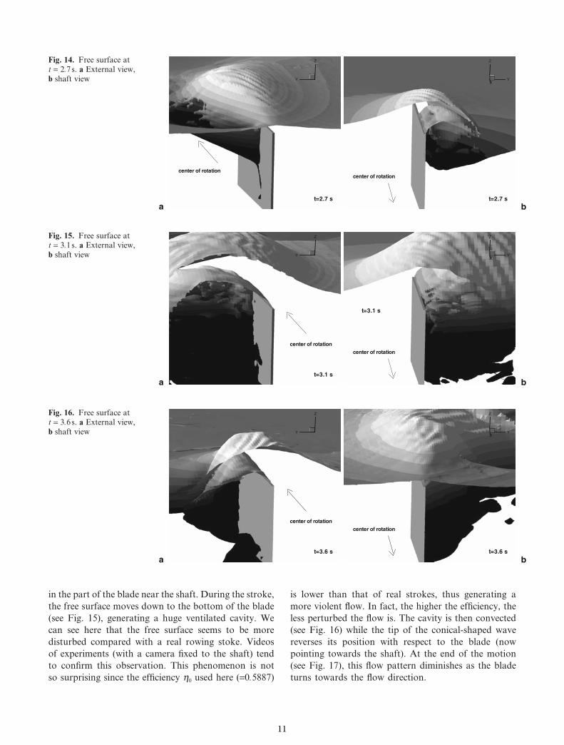
At the beginning of the rotation, it can be observed
in Fig. 12 that there is an elevation of the free surface
just behind the infl ow side of the blade, and conse-
quently a fl ow passing over the upper part of the blade.
Simultaneously, the low-pressure level generated on the
other side of the blade leads to a bowl-shaped cavity
that increases in size. The cavity and the elevation
become more intensifi ed as time (and so q) increases
and the fl ow above the blade gradually takes the shape
of a conical breaking wave (see Figs. 13, 14). It is noted
that this conical wave points towards the external tip
of the blade. The deformation is thus more accentuated
a b
Fig. 11. Horizontal slice
through the M14e5 mesh.
a Top view, b close up of
the region above the blade
XY
Z
t=2.1 s
center of rotation
XY
Z
t=2.1 s
center of rotation
a b
Fig. 12. Free surface at
t = 2.1 s. a External view,
b shaft view
XY
Z
t=2.5 s
center of rotation
XY
Z
t=2.5 s
center of rotation
ba
Fig. 13. Free surface at
t = 2.5 s. a External view,
b shaft view
10
in the part of the blade near the shaft. During the stroke,
the free surface moves down to the bottom of the blade
(see Fig. 15), generating a huge ventilated cavity. We
can see here that the free surface seems to be more
disturbed compared with a real rowing stoke. Videos
of experiments (with a camera fi xed to the shaft) tend
to confi rm this observation. This phenomenon is not
so surprising since the effi ciency h0 used here (=0.5887)
is lower than that of real strokes, thus generating a
more violent fl ow. In fact, the higher the effi ciency, the
less perturbed the fl ow is. The cavity is then convected
(see Fig. 16) while the tip of the conical-shaped wave
reverses its position with respect to the blade (now
pointing towards the shaft). At the end of the motion
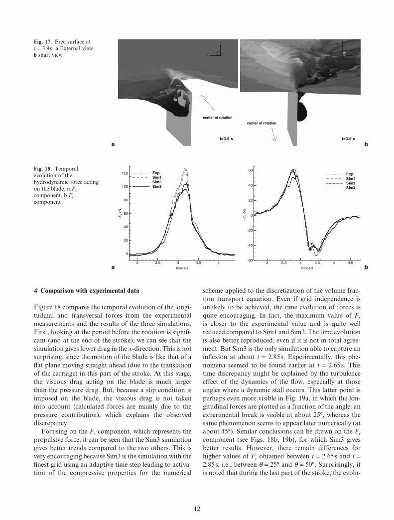
(see Fig. 17), this fl ow pattern diminishes as the blade
turns towards the fl ow direction.
a b
XY
Z
t=2.7 s
center of rotation
XY
Z
t=2.7 s
center of rotation
Fig. 14. Free surface at
t = 2.7 s. a External view,
b shaft view
a b
XY
Z
t=3.1 s
center of rotation
XY
Z
t=3.1 s
center of rotation
Fig. 15. Free surface at
t = 3.1 s. a External view,
b shaft view
a b
XY
Z
t=3.6 s
center of rotation
XY
Z
t=3.6 s
center of rotation
Fig. 16. Free surface at
t = 3.6 s. a External view,
b shaft view
11
4 Comparison with experimental data
Figure 18 compares the temporal evolution of the longi-
tudinal and transversal forces from the experimental
measurements and the results of the three simulations.
First, looking at the period before the rotation is signifi -
cant (and at the end of the stroke), we can see that the
simulation gives lower drag in the x-direction. This is not
surprising, since the motion of the blade is like that of a
fl at plane moving straight ahead (due to the translation
of the carriage) in this part of the stroke. At this stage,
the viscous drag acting on the blade is much larger
than the pressure drag. But, because a slip condition is
imposed on the blade, the viscous drag is not taken
into account (calculated forces are mainly due to the
pressure contribution), which explains the observed
discrepancy.
Focusing on the Fx component, which represents the
propulsive force, it can be seen that the Sim3 simulation
gives better trends compared to the two others. This is
very encouraging because Sim3 is the simulation with the
fi nest grid using an adaptive time step leading to activa-
tion of the compressive properties for the numerical
scheme applied to the discretization of the volume frac-
tion transport equation. Even if grid independence is
unlikely to be achieved, the time evolution of forces is
quite encouraging. In fact, the maximum value of Fx
is closer to the experimental value and is quite well
reduced compared to Sim1 and Sim2. The time evolution
is also better reproduced, even if it is not in total agree-
ment. But Sim3 is the only simulation able to capture an
infl exion at about t = 2.85 s. Experimentally, this phe-
nomena seemed to be found earlier at t = 2.65 s. This
time discrepancy might be explained by the turbulence
effect of the dynamics of the fl ow, especially at those
angles where a dynamic stall occurs. This latter point is
perhaps even more visible in Fig. 19a, in which the lon-
gitudinal forces are plotted as a function of the angle: an
experimental break is visible at about 25°, whereas the
same phenomenon seems to appear later numerically (at
about 45°). Similar conclusions can be drawn on the Fy
component (see Figs. 18b, 19b), for which Sim3 gives
better results. However, there remain differences for
higher values of Fy obtained between t = 2.65 s and t =
2.85 s, i.e., between q = 25° and q = 50°. Surprisingly, it
is noted that during the last part of the stroke, the evolu-
a b
XY
Z
t=3.9 s
center of rotation
XY
Z
t=3.9 s
center of rotation
Fig. 17. Free surface at
t = 3.9 s. a External view,
b shaft view
a btime (s) time (s)
–F
x (N
)
2 2.5 3 3.5 4
0
20
40
60
80
100
120 Exp.
Sim1
Sim2
Sim3
–F
y (N
)
2 2.5 3 3.5 4 4.5-60
-40
-20
0
20
40
60Exp.
Sim1
Sim2
Sim3
Fig. 18. Temporal
evolution of the
hydrodynamic force acting
on the blade. a Fx
component, b Fy
component
12
tion is very well captured, especially when the forces stop
decreasing at about t = 3.3 s. Comparison of the z-axis
torque shows similar behaviour. Fairly good agreement
is observed, apart from the angular zone between 25°
and 50°. Here again, it seems that the break observed in
the measured increase of Mz at q = 25° and t = 2.65 s
occurs about 0.2 s later in the simulation. In conclusion,
we can say that the phenomenon observed experimen-
tally at t = 2.65 s, (which results in a break on the evolu-
tion of forces Fx and Fy), is not yet accurately captured
by the simulations. In fact, it seems to occur later numer-
ically (for the more precise simulation Sim3). These dif-
ferences could perhaps be explained by too coarse a grid
even on the M14e5 mesh and also by the infl uence of the
turbulence effect on pressure and then on the free-surface
elevation, especially when a dynamic stall occurs. It can
also be noted in Fig. 6 that, after t = 2.6 s (up to t = 3.0 s),
the difference between the analytical law (qa) prescribed
by the simulation and the real measured angle (qm) varies
rapidly. It locally leads to a difference of about 0.4 ° s−1
for the angular velocity, which is surely too small to
explain the observed gap between the measured and
simulated forces.
Figure 21 plots the quantity dip over half a blade
length (denoted by Lhb). As point P is the localization
where the resultant force acts, this fi gure shows that the
migration of this point towards the shaft of the blade is
accurately calculated. Finally, Figs. 22 and 23 concern
the effi ciencies. At the beginning of the stroke, it can be
seen that the main difference between h and h0 is mainly
a bq (deg)
–F
x (N
)
0 20 40 60 80 100 120 140 160 180
0
20
40
60
80
100
120 Exp.
Sim1
Sim2
Sim3
q (deg)
–F
y (N
)
0 20 40 60 80 100 120 140 160 180-60
-40
-20
0
20
40
60
Exp.
Sim1
Sim2
Sim3
Fig. 19. Hydrodynamic
force on the blade as a
function of the angle of
rotation q. a Fx
component, b Fy
component
a btime (s)
–M
z (N
)
2 3 4
0
20
40
60
80
100
120
140
160 Exp.
Sim1
Sim2
Sim3
q (deg)
–M
z (N
)
0 20 40 60 80 100 120 140 160 180
0
20
40
60
80
100
120
140
160 Exp.
Sim1
Sim2
Sim3
Fig. 20. Hydrodynamic
z-axis torque (Mz) on the
blade at point O. a Mz as a
function of time, b Mz as a
function of angle
q (deg)
dip
/ L
hb
20 40 60 80 100 120 140 160-0.8
-0.6
-0.4
-0.2
0
0.2
0.4
0.6
Exp.
Sim3
Fig. 21. Evolution of the dip/Lhb ratio
13
due to hf , i.e., the orientation of the hydrodynamics with
respect to the perpendicular direction of the blade. As
Eq. 5 shows, this orientation has all the more infl uence
on h as q deviates from p/2. For the range of angles cor-
responding to the fi rst part of the stroke (just after the
catch), b is negative, i.e., the orientation of the force is
unfavourable for propulsion. The propulsion is then
lower than if the force were directed along n. The differ-
ence between the simulation and experiment here is
found to result from quite a large discrepancy in hf in
the fi rst part of the stroke, whereas the evolution of hp
is in good agreement with measurements. As noted pre-
viously, the position of point P is actually well captured
by the simulation. It is also seen that this coeffi cient hp
remains close to 1 during a large part of the stroke
(hp ∈ [0.94, 1.01] for q ∈ [40°, 140°]).
Figure 23 fi nally shows that h0 can actually be con-
sidered the dominant parameter for such a stroke
between q = 40° and q = 140°, corresponding to the effec-
tive propulsive phase for oarsmen. Here again, quite a
large gap between the experimental and numerical effi -
ciency h is visible in the fi rst part of the stroke (mainly
due to the component hf , as remarked previously). For
angles less than about 20°, the difference is quite large,
because the viscous contribution to Fx (which cannot be
captured by the simulation since a slip condition is
imposed on the blade) remains quite large compared to
the pressure effect. In contrast, it does not infl uence Fy
similarly since the latter is mainly produced by the pres-
sure effect when q is small. As a result, the angle b (and
so hf) cannot be precisely evaluated in this case.
5 Conclusions
The fl ow around an oar blade is very complex, especially
because a human is part of the system. From the hydro-
dynamics point of view, it is an unsteady 3-D fl ow
including violent free-surface motion and overturning.
From the kinematics point of view, the motion of the
blade results in a variable translation of the boat
coupled to a rotation of the shaft and a vertical move-
ment of the blade (even if in the present analysis, the
latter is not taken into account). To investigate the fl ow
and to improve the modelling of the forces acting on
a blade (as part of a simulator for a complete boat–
oarsmen–oars system), a device reproducing a simplifi ed
rowing stroke was designed and built. The chosen kine-
matics are not excessively restrictive and give a reliable
database to validate the numerical approach. The
numerical simulations presented here demonstrate the
capacity to deal with such a complex fl ow, especially
since the present work uses a low-effi ciency movement
that produces a more violent fl ow than that of a real
rowing stroke. Even if grid convergence is not obtained
and turbulence is not yet taken into account, compari-
sons with experimental data are very encouraging and
give confi dence in the capacity of the numerical method
to simulate accurately such a fl ow pattern. The fact that
the elevation and the shape of the free surface exten-
sively change during the stroke makes the task more
diffi cult. As a matter of fact, the whole part of the
domain in which the interface takes place has to be
gridded with fi ne cells. Without a local adaptive grid
procedure, meshes with a huge number of cells are
needed and simulations are hampered by a lot of useless
fi ne cells. As has already been found by Hay et al.,18,19
the development of a fully parallelized local mesh refi ne-
ment procedure with dynamic load balancing should
decrease dramatically the processing time, while keeping
the generality of the approach. With this technique,
a bq (deg)
hf
20 40 60 80 100 120 140 160
0.7
0.8
0.9
1
Exp.
Sim3
q (deg)
hp
20 40 60 80 100 120 140 160
0.9
0.95
1
1.05
1.1
Exp.
Sim3
Fig. 22. Evolution of
effi ciencies hf (a) and hp
(b). The effi ciencies are
defi ned in Eq. 5
q (deg)
h
0 20 40 60 80 100 120 140 160 1800
0.2
0.4
0.6
0.8
η : Sim3
η : Exp.
η0
Fig. 23. Comparison of effi ciency h with respect to h0
14
accurate simulations might be performed within a rea-
sonable time. When this technique is operational and
the processing time far shorter, new simulations will be
performed for other experimental data of an oar with
a rigid shaft. Comparisons with available data from real
oars realized with the experimental device could also
be added. Then, it will be possible to study the infl uence
of oar deformation. Once simulations are validated with
these towing tank tests, numerical simulations for a
realistic confi guration will be relevant and will become
far easier than experimental approaches. Indeed, the
study of complex movements with variable immersion
(with catch and fi nish) and with a variable speed of
translation taken into account will become much easier
than carrying out tests experimentally. The last step will
then be validation by real rowing tests, which we have
been carrying out for several years with instrumented
oars and measurement equipment on the boat to record
the oar and oarsman kinematics. With the numerical
results of parametric studies on oars (e.g., stiffness, lever
length, and shape of the blade) and movement charac-
teristics, we will be able to replace empirical indications
by objective and unbiased criteria not only for oars but
also for the rowing style. Furthermore, a detailed analy-
sis and comparison of the fl ow topology for some
selected and typical results could then be started to pre-
cisely understand the physical mechanism involved in
such a complex confi guration. The knowledge gathered
in these fi elds and from such models as a result of these
studies will be then progressively integrated into the
global simulator.
Acknowledgments. The authors gratefully acknowledge the scien-
tifi c committee of CINES (project dmn2049) and IDRIS (project
0129) for the attribution of computer time.
References
1. Wellicome JF (1967) Some hydrodynamic aspects of row-
ing. In: Williams JGP, Scott AC (eds) Rowing, a scientifi c
approach. Barnes, New York
2. Videv TA, Doi Y (1993) Unsteady viscous fl ow simulation
around the blade of a rowing boat. J Soc Naval Archit Jpn
173:97–108
3. Barré S, Kobus JM (1998) New facilities for measurement and
modelling of hydrodynamic loads on oar blades. In: Haake SJ
(ed) The engineering of sport. Blackwell
4. Pope DL (1973) On the dynamics of men and boat and oars.
In: Bleustein JL (ed) Mechanics and sport. ASME, New York,
pp 113–130
5. Barré S (1998) Etude expérimentale des systèmes de pro-
pulsion instationnaire. Application aux palettes d’aviron.
PhD Thesis, University of Nantes/Ecole Centrale de Nantes,
France
6. Spalart PR, Allmaras SR (1992) A one-equation turbulence
model for aerodynamic fl ows. AIAA 30th Aerospace Sciences
Meeting. Reno, NV, AIAA Paper 92-0439
7. Menter FR (1993) Zonal two-equation k −w turbulence models
for aerodynamic fl ows. IAIAA 24th Fluid Dynamic Confer-
ence. Orlando, FL, AIAA Paper 93-2906
8. Duvigneau R, Visonneau M, Deng GB (2003) On the role
played by turbulence closures for hull shape optimization at
model and full scale. J Mar Sci Technol 8:11–25
9. Jasak H, Weller HG, Gosman AD (1999) High-resolution
NVD differencing scheme for arbitrarily unstructured meshes.
Int J Numer Methods Fluids 31:431–449
10. Pržulj V, Basara B (2001) Bounded convection schemes for
unstructured grids. In: Proceedings of the AIAA 15th compu-
tational fl uid dynamics conference. Anaheim, CA, AIAA
paper 2001-2593
11. Jasak H, Weller HG (1995) Interface tracking capabilities of
the inter-gamma differencing scheme. Internal report, CFD
research group, Imperial College, London
12. Leonard B (1988) Simple high-accuracy resolution program
for convective modelling of discontinuities. Int J Numer
Methods Fluids 8:1291–1318
13. Gaskell PH, Lau AKC (1988) Curvature compensated convec-
tive transport: Smart, a new boundedness-preserving trans-
port algorithm. Int J Numer Methods Fluids 8:617–641
14. Queutey P, Visonneau M (2007) An interface-capturing
method for free-surface hydrodynamic fl ows. Comput Fluids
36:1481–1510
15. Leroyer A (2004) Fluid/motion interaction for solid and fl exi-
ble bodies by resolution of the Navier–Stokes equations.
Contribution to the numerical modelling of cavitating fl ows.
PhD Thesis, University of Nantes/Ecole Centrale de Nantes,
France. Can be downloaded (in French) at ftp://ftpa.ec-nantes.
fr/pub/DMN/Thesis/these_leroyer.pdf
16. Ferziger JH, Peri´c M (2002) Computational methods for fl uid
dynamics, 3rd edn. Springer-Verlag, Berlin
17. Leroyer A, Visonneau M (2005) Numerical methods for
RANSE simulations of a self-propelled fi shlike body. J Fluids
Struct 20:975–991
18. Hay A, Leroyer A, Visonneau M (2006) H-adaptive Navier–
Stokes simulations of free-surface fl ows around moving
bodies. J Mar Sci Technol 11:1–18
19. Hay A, Visonneau M (2005) Computation of free-surface
fl ows with local mesh adaptation. Int J Numer Methods Fluids
49:785–816
15
Copyright © 2022 FDOKUMEN