
Investigation of propeller characteristics at low Reynolds ...
89
Investigation of pro- peller characteristics at low Reynolds num- ber with an angle of attack A computational aeroacoustic study Akash Pandey Master of Science Thesis
-
Upload
khangminh22 -
Category
Documents
-
view
1 -
download
0
Transcript of Investigation of propeller characteristics at low Reynolds ...
Investigation of pro-peller characteristicsat low Reynolds num-ber with an angle ofattackA computational aeroacoustic study
Akash Pandey
Master of Science Thesis


Investigation of propellercharacteristics at low
Reynolds number with anangle of attack
A computational aeroacoustic studyby
Akash Pandey
to obtain the degree of Master of Scienceat the Delft University of Technology,
to be defended publicly on Wednesday, 7 of April, 2021.
Student number: 4792955Research group : Aeroacoustics group, Aerodynamics and Wind Energy trackThesis committee: Prof. dr. D. Casalino, TU Delft, chair
Dr. F. Avallone, TU Delft, supervisorDr. D. Ragni, TU Delft, supervisorG. Romani, TU Delft, supervisorDr. T. Sinnige, TU Delft, external examiner
An electronic version of this thesis is available at http://repository.tudelft.nl/.


Acknowledgement”Hard times create strong people, strong people create good times.”
-G. Michael Hopf
It is how I would like to summy experience of doing the thesis and my hopes for the future. Doing mymaster’s thesis in the middle of a pandemic with the entire aviation industry in shambles was perhapsnever a part of my worst nightmare. Add to it the feeling of isolation and uncertainty coupled with myextroverted nature, and you have a recipe for disaster. Yet here we are, reading the acknowledgmentsection of my master’s thesis. So I guess these are some very special people, without whom this thesiscouldn’t have been possible.
First of all, thank you to my family, mummy, papa, Aman. Despite being on three different continents,we never got distant. It is hard to put in words all that you have done for me. But all I can say is I owe allmy success to your support. Shreyas and, Arpit thank you for being there no matter the time or placeyou guys have become family over the years. The Discord sessions and calls with you made work fromhome more bearable. My housemates Agnieszka, Kristyna, John, and Lilly, thank you for creating ahome away from home and making the lockdown fun. Dr. Vinit and Ankur bhaiya for being the guidinglights of my journey in Delft. Both of you inspire me with your can-do attitude and deep knowledge ofyour respective fields. I have learned so much from you, and I sincerely hope it continues to be thisway. My friends from Delft Abhratej, Anshita, Athreya, Hrishikesh, Haris, and Shubham. It was a delightworking with you on the courses, having light-hearted discussions, and getting valuable feedback. Delftwouldn’t have been the same without you.
A big thank you to James, Ruben, Quint, Alex, Thom, Tom, Victor, Teresa, and all the other team-mates at Silverwing. My best memories from Delft are with you guys. It was an absolute delightworking, playing, and doing all sorts of random stuff with you guys. Making the aircraft has been oneof the most enriching experiences of my life and was a great motivation in further exploring the field ofaeroacoustics.
At TU Delft, I would like to extend my sincerest gratitude to Dr. Francesco Avallone for his guidance,support, and patience. Working with him has helped me develop a more critical attitude and an eyefor detail. I am also thankful to Dr. Daniele Ragni and Gianluca, for providing their valuable inputs andenabling me to improve my work. It was a pleasure working with you and learning from you.
Lastly, I would like to acknowledge the role of COVID-19 in my thesis. Thank you for giving me somuch time in isolation with my thoughts, thank you for making it so hard, and thank you for making merealize that I can do it. To close the loop, I would like to end with another quote that sums up all mylearnings so far:
”The hardest battles that you would ever fight is with yourself.”
Akash PandeyDelft, 2021
iii

SummaryAdvancements in technology have made commercial unmanned aerial vehicles reliable and readily
available, leading to an exponential rise in their market demand over the past few years. COVID-19 has further accelerated this growth through an increase in demand for contact-less delivery andcrowd monitoring systems. However, despite these favorable conditions, their limited range, perceivedthreat, and concerns about noise pollution in urban environments have prevented them from beingwidely accepted by society. A recent study by NASA [1] found that people perceive UAV noise to bemore annoying than cars, and trucks at a similar sound pressure level, which highlights the need tounderstand the acoustic characteristic of these aircraft.
These UAVs are generally powered by electric motors, making their propellers the most dominantsource of noise. In the past, researchers have conducted several studies to understand and charac-terize the noise produced by aircraft propellers. However, these studies were limited to high Reynolds(> 10 ) and Mach number operations for large commercial aircraft, creating a significant gap in theunderstanding of the aerodynamic and acoustic characteristics of propellers operating at low Reynolds(< 2∗10 ) and Mach number. This thesis aims to address the research gap by performing a high-fidelitycomputational simulation using Dassault Systèmes PowerFLOW®. The tool uses a lattice Boltzmann-very large eddy simulation (LBM-VLES) based approach to compute the aerodynamic results and theFfowcs-Williams and Hawkings (FWH) aeroacoustic analogy to calculate far-field acoustic values. Themain objective of the thesis is:
“To characterize andquantify the effect of non-axisymmetric inflowconditionson theaerodynamicandacousticpropertiesofpropellersoperatingat lowReynoldsnumbers.”
To meet the objective, a computational setup consisting of a twin-bladed propeller with a radius of15 𝑐𝑚 is designed in PowerFLOW®. The propeller is analyzed at 0 and 15 AoA, operating at 6000RPM with a freestream velocity of 12 𝑚/𝑠𝑒𝑐 and the results validated against experimental data.
Aerodynamic measurements and flow analysis revealed that the change in angle of attack (AoA)resulted in a 3.87% increase in the net thrust, and 1.16% increase in the net torque value of the propeller.Operating at an AoA, the propeller blade experiences asymmetric loading around the propeller plane,the loads fluctuate by 35% between the points of maximum and minimum loading. Further analysisof the propeller flow field is carried out by averaging the velocity field and performing a phase-lockedanalysis to visualize the vortex field. The analysis helps in understanding the effect of AoA on propellerwake and quantifies its asymmetric nature.
Far-field acoustic data is acquired by two circular microphone arrays, with a polar angle resolutionof 10 . The arrays are placed around the propeller plane and along the axial axis of the propeller. Thechange in AoA results in a 3 𝑑𝐵 higher noise at an azimuthal angle (Ψ) of 90 and reduces by an equalmagnitude at Ψ = 270 . The shift is attributed to the change in propeller tip Mach number and localblade AoA as a function of its azimuthal location and propeller AoA. Further analysis of the sound powerlevel (PWL) produced by the propeller is carried out, showing a 1.5 𝑑𝐵 increase in the PWL producedby the propeller blade at 15 AoA than 0 .
iv

Contents
Acknowledgement iii
Summary iv
List of Abbreviations vii
List of Symbols viii
List of Figures x
List of Tables xii
1 Introduction 11.1 Research objective . . . . . . . . . . . . . . . . . . . . . . . . . . . . . . . . . . . . . . . 21.2 Approach . . . . . . . . . . . . . . . . . . . . . . . . . . . . . . . . . . . . . . . . . . . . 21.3 Outline of thesis . . . . . . . . . . . . . . . . . . . . . . . . . . . . . . . . . . . . . . . . 3
2 Theoretical Background 42.1 Propeller aerodynamics . . . . . . . . . . . . . . . . . . . . . . . . . . . . . . . . . . . . 42.2 Sound . . . . . . . . . . . . . . . . . . . . . . . . . . . . . . . . . . . . . . . . . . . . . . 6
2.2.1 Sources of sound . . . . . . . . . . . . . . . . . . . . . . . . . . . . . . . . . . . . 62.2.2 Measurement of sound. . . . . . . . . . . . . . . . . . . . . . . . . . . . . . . . . 8
2.3 Aeroacoustics. . . . . . . . . . . . . . . . . . . . . . . . . . . . . . . . . . . . . . . . . . 92.3.1 Propeller noise . . . . . . . . . . . . . . . . . . . . . . . . . . . . . . . . . . . . . 92.3.2 Airfoil noise generation mechanism . . . . . . . . . . . . . . . . . . . . . . . . . . 10
2.4 Aeroacoustic analogies . . . . . . . . . . . . . . . . . . . . . . . . . . . . . . . . . . . . 112.4.1 Lighthill’s acoustic analogy. . . . . . . . . . . . . . . . . . . . . . . . . . . . . . . 122.4.2 Ffowcs-Williams and Hawkings (FWH) analogy . . . . . . . . . . . . . . . . . . . 13
3 Literature Review 143.1 Fundamental research . . . . . . . . . . . . . . . . . . . . . . . . . . . . . . . . . . . . . 14
3.1.1 Radial directivity . . . . . . . . . . . . . . . . . . . . . . . . . . . . . . . . . . . . 153.1.2 Axial directivity . . . . . . . . . . . . . . . . . . . . . . . . . . . . . . . . . . . . . 17
3.2 Low Reynolds number . . . . . . . . . . . . . . . . . . . . . . . . . . . . . . . . . . . . . 193.2.1 Aerodynamic research . . . . . . . . . . . . . . . . . . . . . . . . . . . . . . . . . 193.2.2 Aeroacoustic research . . . . . . . . . . . . . . . . . . . . . . . . . . . . . . . . . 20
3.3 Research questions . . . . . . . . . . . . . . . . . . . . . . . . . . . . . . . . . . . . . . 22
4 Methodology 244.1 Lattice Boltzmann method . . . . . . . . . . . . . . . . . . . . . . . . . . . . . . . . . . . 24
4.1.1 Principle of LBM: . . . . . . . . . . . . . . . . . . . . . . . . . . . . . . . . . . . . 244.1.2 Choice of LBM . . . . . . . . . . . . . . . . . . . . . . . . . . . . . . . . . . . . . 25
4.2 LBM implementation in the flow solver . . . . . . . . . . . . . . . . . . . . . . . . . . . . 264.2.1 Algorithm . . . . . . . . . . . . . . . . . . . . . . . . . . . . . . . . . . . . . . . . 264.2.2 Turbulence model . . . . . . . . . . . . . . . . . . . . . . . . . . . . . . . . . . . 274.2.3 Boundary condition . . . . . . . . . . . . . . . . . . . . . . . . . . . . . . . . . . . 274.2.4 Grid generation . . . . . . . . . . . . . . . . . . . . . . . . . . . . . . . . . . . . . 28
4.3 Aeroacoustic solver . . . . . . . . . . . . . . . . . . . . . . . . . . . . . . . . . . . . . . 294.3.1 FWH analogy implementation . . . . . . . . . . . . . . . . . . . . . . . . . . . . . 304.3.2 Acoustic signal sampling . . . . . . . . . . . . . . . . . . . . . . . . . . . . . . . . 31
v

vi Contents
5 Setup 325.1 Geometry . . . . . . . . . . . . . . . . . . . . . . . . . . . . . . . . . . . . . . . . . . . . 32
5.1.1 Coordinate System . . . . . . . . . . . . . . . . . . . . . . . . . . . . . . . . . . . 335.1.2 Blade tripping . . . . . . . . . . . . . . . . . . . . . . . . . . . . . . . . . . . . . . 34
5.2 Resolution . . . . . . . . . . . . . . . . . . . . . . . . . . . . . . . . . . . . . . . . . . . 355.2.1 VR Regions . . . . . . . . . . . . . . . . . . . . . . . . . . . . . . . . . . . . . . . 37
5.3 Acoustic measurement . . . . . . . . . . . . . . . . . . . . . . . . . . . . . . . . . . . . . 385.4 Simulation settings . . . . . . . . . . . . . . . . . . . . . . . . . . . . . . . . . . . . . . . 39
5.4.1 Global parameters . . . . . . . . . . . . . . . . . . . . . . . . . . . . . . . . . . . 395.4.2 Boundary Conditions . . . . . . . . . . . . . . . . . . . . . . . . . . . . . . . . . . 405.4.3 Time convergence . . . . . . . . . . . . . . . . . . . . . . . . . . . . . . . . . . . 405.4.4 Measurements . . . . . . . . . . . . . . . . . . . . . . . . . . . . . . . . . . . . . 40
5.5 Experimental setup . . . . . . . . . . . . . . . . . . . . . . . . . . . . . . . . . . . . . . . 42
6 Resolution Study 436.1 Aerodynamic study . . . . . . . . . . . . . . . . . . . . . . . . . . . . . . . . . . . . . . . 436.2 Aeroacoustic study . . . . . . . . . . . . . . . . . . . . . . . . . . . . . . . . . . . . . . 45
6.2.1 FWH surface selection . . . . . . . . . . . . . . . . . . . . . . . . . . . . . . . . . 466.2.2 Grid selection . . . . . . . . . . . . . . . . . . . . . . . . . . . . . . . . . . . . . . 48
7 Results 517.1 Propeller force . . . . . . . . . . . . . . . . . . . . . . . . . . . . . . . . . . . . . . . . . 517.2 Flow field analysis . . . . . . . . . . . . . . . . . . . . . . . . . . . . . . . . . . . . . . . 52
7.2.1 Velocity field . . . . . . . . . . . . . . . . . . . . . . . . . . . . . . . . . . . . . . 537.2.2 Vortex field . . . . . . . . . . . . . . . . . . . . . . . . . . . . . . . . . . . . . . . 557.2.3 Surface pressure fluctuation . . . . . . . . . . . . . . . . . . . . . . . . . . . . . . 56
7.3 Acoustics . . . . . . . . . . . . . . . . . . . . . . . . . . . . . . . . . . . . . . . . . . . . 577.3.1 Source noise . . . . . . . . . . . . . . . . . . . . . . . . . . . . . . . . . . . . . . 587.3.2 Radial directivity . . . . . . . . . . . . . . . . . . . . . . . . . . . . . . . . . . . . 597.3.3 Axial directivity . . . . . . . . . . . . . . . . . . . . . . . . . . . . . . . . . . . . . 60
8 Conclusions and Recommendations 628.1 Conclusions. . . . . . . . . . . . . . . . . . . . . . . . . . . . . . . . . . . . . . . . . . . 628.2 Recommendations . . . . . . . . . . . . . . . . . . . . . . . . . . . . . . . . . . . . . . . 64
A Appendix 65
B Appendix 70
Bibliography 72

List of AbbreviationsAoA Angle of attack
BC Boundary condition
BPF Blade passing frequency
BVI Blade vortex interaction
CAA Computational aeroacoustics
CFD Computational fluid dynamics
FWH Ffowcs-Williams and Hawkings
FWH SLD Ffowcs-Williams and Hawkings solid integration surface
FWH PRM Ffowcs-Williams and Hawkings permeable integration surface
ICAO International Civil Aviation Organization
LBM Lattice Boltzmann method
LHS Left hand side
LRF Local rotating reference frame
OASPL Overall sound pressure level
NS Navier-Stokes
PAVs Personal aerial vehicle
PS Power spectrum
PSD Power spectral density
PWL Sound power level
RHS Right hand side
RPM Rounds per minute
SPL Sound pressure level
SR Single-rotating propellers
TR Total reaction
UAVs Unmanned aerial vehicle
VR Variable resolution
VTOL Vertical takeoff and landing
STOL Short takeoff and landing
vii

List of Symbols
Greek Symbols𝛼 Angle of attack ( )
𝛽 Blade pitch angle ( )
𝜂 Efficiency
𝜃 Axial angle ( )
𝜆 Wavelength (𝑚)
𝜌 Density (𝐾𝑔/𝑚 )
𝜙 Radiation angle ( )
Ψ Azimuthal angle of propeller ( )
𝜔 Vorticity magnitude (𝐻𝑧)
Latin SymbolsB Number of propeller blades
𝐶 Coefficient of drag
𝐶 Coefficient of lift
𝐶 Coefficient of thrust
𝐶 Coefficient of torque
𝐷 Diameter (𝑚)
𝑑𝐵 Decibel
𝑓 Frequency (𝐻𝑧)
J Bessel function of the first kind
𝐽 Advance ratio
𝑘 Wave number
𝐾 Kelvin
𝑙 Characteristic length (𝑚𝑚)
𝑀 Mach number
𝑛 Rotations per second (1/𝑠𝑒𝑐)
𝑁 Newtons
N Number of blades
𝑝 Pressure (𝑃𝑎)
viii

List of Symbols ix
𝑃 Power (𝑊)
𝑟 Sectional radius (𝑚𝑚)
𝑅 Propeller radius (𝑚)
𝑄 Torque (𝑁𝑚)
𝑅𝑒 Reynolds number
𝑡 Time (𝑠𝑒𝑐)
𝑇 Temperature (K)
𝑈 Freestream fluid velocity (𝑚/𝑠𝑒𝑐)
List of Figures
1.1 Drones performing aerial delivery of medical supplies; A hybrid tilt rotor UAV (left) and afixed wing delivery drone (right) . . . . . . . . . . . . . . . . . . . . . . . . . . . . . . . . 1
2.1 Propellers and rotors . . . . . . . . . . . . . . . . . . . . . . . . . . . . . . . . . . . . . . 42.2 Force experience by a propeller at an AoA . . . . . . . . . . . . . . . . . . . . . . . . . . 52.3 Change in Propeller efficiency vs advance ratio at specific blade AoA [2] . . . . . . . . . 52.4 Compression and expansion of air due to propagation of sound waves [3] . . . . . . . . 62.5 Radiation pattern of different sound sources [4] . . . . . . . . . . . . . . . . . . . . . . . 72.6 Effective Sound pressure and corresponding SPL in decibel scale [5] . . . . . . . . . . . 82.7 Weighting graph for sound pressure levels [6] . . . . . . . . . . . . . . . . . . . . . . . . 92.8 Converting pressure signal from a propeller analysis to power spectrum . . . . . . . . . 92.9 Pressure signal produced by a propeller; Tonal component (top left), Broadband compo-
nent (bottom left), and total pressure signal (right); adapted from [7] . . . . . . . . . . . 102.10 Turbulent boundary layer trailing edge noise [8] . . . . . . . . . . . . . . . . . . . . . . . 112.11 Separation and stall noise [8] . . . . . . . . . . . . . . . . . . . . . . . . . . . . . . . . . 11
3.1 Visualisation of propeller disc AoA; adapted from [9] . . . . . . . . . . . . . . . . . . . . 153.2 Variation in propeller blade properties with AoA (𝛼) at Ψ = 90 . . . . . . . . . . . . . . 153.3 Experimental setup and radial noise directivity [10] . . . . . . . . . . . . . . . . . . . . . 163.4 Radial noise directivity at 1 BPF of a 4 bladed SR-2 propeller at 9 AoA wrt. 0 base
line; Operating condition 𝑀 = 0.4 freestream velocity 30 𝑚/𝑠𝑒𝑐 [11] . . . . . . . . . . 163.5 Radial noise directivity at 1 BPF of a 4 bladed SR-2 propeller at 9 AoA wrt. 0 base
line at a freestream velocity 30 𝑚/𝑠𝑒𝑐 [12] . . . . . . . . . . . . . . . . . . . . . . . . . . 173.6 Propeller noise directivity pattern for axial inflow condition . . . . . . . . . . . . . . . . . 183.7 Experimental setup and propeller noise directivity at 0 AoA [10] . . . . . . . . . . . . . 183.8 Effect of AoA on axial directivity of BPF [10] . . . . . . . . . . . . . . . . . . . . . . . . . 183.9 Impact of 𝑅𝑒 on airfoil characteristics . . . . . . . . . . . . . . . . . . . . . . . . . . . . . 193.10 Impact of 𝑅𝑒 on airfoil characteristics . . . . . . . . . . . . . . . . . . . . . . . . . . . . . 203.11 Power spectrum plot for at constant thrust of 2.8 N [13]. . . . . . . . . . . . . . . . . . . 213.12 Experimental setup and impact of rotor airframe separation on propeller noise [14] . . . 213.13 Schematics of the experimental setup along with rotor coordinates [15] . . . . . . . . . . 223.14 Noise spectra for different free stream velocity and AOA [15] . . . . . . . . . . . . . . . 22
4.1 Discrete lattice nodes in D2Q9 model (left([16]) and D3Q19 model (right [17]). . . . . . 254.2 Computational Steps - 𝐷2𝑄9 from propagation to collision [17] . . . . . . . . . . . . . . 274.3 On-grid implementation of bounce Back BC [16] . . . . . . . . . . . . . . . . . . . . . . 284.4 Zou-He BC [16] . . . . . . . . . . . . . . . . . . . . . . . . . . . . . . . . . . . . . . . . . 284.5 Elements of a lattice in PowerFLOW® [18] . . . . . . . . . . . . . . . . . . . . . . . . . . 294.6 Voxel size dependence on VR region, adapted from [18] . . . . . . . . . . . . . . . . . . 294.7 Grid generation for rotating bodies [18] . . . . . . . . . . . . . . . . . . . . . . . . . . . . 304.8 Well sampled signal (top) vs aliased signal due to under-sampling (bottom) . . . . . . . 31
5.1 Propeller chord length and blade angle vs blade span (r/R) . . . . . . . . . . . . . . . . 325.2 Propeller blade before (top) and after (bottom) being processed by 𝑂𝑝𝑡𝑦𝜕𝑏® . . . . . . 335.3 Complete geometry of the propeller setup . . . . . . . . . . . . . . . . . . . . . . . . . . 335.4 Coordinate system with respect to the propeller geometry . . . . . . . . . . . . . . . . . 345.5 Zig-Zag trip on propeller blade . . . . . . . . . . . . . . . . . . . . . . . . . . . . . . . . 355.6 Change in grid size with VR region; VR region in close proximity of propeller setup (left)
and VR region closer to the propeller blade (right) . . . . . . . . . . . . . . . . . . . . . 36
x

List of Figures xi
5.7 Variable resolution regions; propeller surface (red), propeller wake (green) and far field(blue) . . . . . . . . . . . . . . . . . . . . . . . . . . . . . . . . . . . . . . . . . . . . . . 37
5.8 Variable resolution regions; VR 12 (yellow) VR 11 (Pink) . . . . . . . . . . . . . . . . . . 385.9 Acoustic setup of the simulation; 3 FWH permeable surface (red), VR 10 (green) . . . . 395.10 Time convergence of 𝐶 value at medium resolution at 0 AoA . . . . . . . . . . . . . . 415.11 Fluid measurement setup; transient measurement volume (pink), VR 10 (green) . . . . 415.12 Experimental Setup . . . . . . . . . . . . . . . . . . . . . . . . . . . . . . . . . . . . . . 42
6.1 Variation of 𝐶 value with grid resolution . . . . . . . . . . . . . . . . . . . . . . . . . . . 446.2 Vortex visualization for different resolution at Λ = −1 ∗ 10 1/sec for 𝛼 = 15 ; Suction
side of propeller blade. . . . . . . . . . . . . . . . . . . . . . . . . . . . . . . . . . . . . . 446.3 Variation of 𝐶 value with grid resolution . . . . . . . . . . . . . . . . . . . . . . . . . . . 456.4 Difference in OASPL between solid and permeable FWH integration surface . . . . . . 466.5 Power spectrum of solid and permeable FWH integration surface; Δ𝑓 = 20 𝐻𝑧 . . . . . . 476.6 Comparison between solid (SLD), permeable (PRM), and experimental (EXP) noise data
at 15 AoA . . . . . . . . . . . . . . . . . . . . . . . . . . . . . . . . . . . . . . . . . . . 486.7 Variation in acoustic result with grid resolution at 𝛼 = 0 . . . . . . . . . . . . . . . . . . 496.8 Surface pressure fluctuation (𝑑𝐵) at 0 AoA for a frequency range of 1, 500 − 2, 500 𝐻𝑧;
contour range 60 dB, suction side of the propeller blade. . . . . . . . . . . . . . . . . . . 50
7.1 Variation in sectional 𝐶 and 𝐶 with azimuthal angle (Ψ) for 𝛼 = 0 and 15 . . . . . . . 527.2 Change in thrust values with azimuthal angle (Ψ) . . . . . . . . . . . . . . . . . . . . . . 537.3 Axial velocity profile for 0 and 15 AoA . . . . . . . . . . . . . . . . . . . . . . . . . . . 537.4 Velocity magnitude at different radial position along the propeller axis . . . . . . . . . . 547.5 Vorticity magnitude along the propeller axis . . . . . . . . . . . . . . . . . . . . . . . . . 557.6 Vortex visualization for 0 and 15 AoA at Λ = −1 ∗ 10 1/𝑠𝑒𝑐 and Ψ = 0 . . . . . . 567.7 Surface pressure fluctuation (𝑑𝐵) at 1 , 2 and 3 BPF; contour range 60 𝑑𝐵 . . . . 577.8 Surface pressure fluctuation (𝑑𝐵) between 1, 500−7, 500𝐻𝑧 at 1, 000 𝐻𝑧 interval; contour
range 60 𝑑𝐵. . . . . . . . . . . . . . . . . . . . . . . . . . . . . . . . . . . . . . . . . . . 587.9 Sound power level across a the propeller blade . . . . . . . . . . . . . . . . . . . . . . . 587.10 Radial directivity of OASPL; frequency range a) 40 − 1, 000 𝐻𝑧 b) 1, 000 − 10, 000 𝐻𝑧 c)
40 − 10, 000 𝐻𝑧; measured at 1 𝑚 from the propeller axis of rotation; . . . . . . . . . . 597.11 Variation in spectrum level around the propeller plane . . . . . . . . . . . . . . . . . . . 607.12 Axial directivity of OASPL; frequency range a) 40 − 1, 000 𝐻𝑧 b) 1, 000 − 10, 000 𝐻𝑧 c)
40 − 10, 000 𝐻𝑧; measured at 1 𝑚 from the propeller axis of rotation; . . . . . . . . . . 617.13 Variation in noise spectra along the axial direction . . . . . . . . . . . . . . . . . . . . . 61
A.1 NASA SR series propeller blades[8] . . . . . . . . . . . . . . . . . . . . . . . . . . . . . 66A.2 Simulating AoA in the computational setup . . . . . . . . . . . . . . . . . . . . . . . . . 66A.3 Variation in AoA and resultant velocity for propellers with an AoA . . . . . . . . . . . . . 67A.4 Difference between FWH SLD and the the three individual FWH PRM surface . . . . . . 68A.5 Average change in AoA across blade span. . . . . . . . . . . . . . . . . . . . . . . . . . 68A.6 Mean axial velocity profile in the propeller slipstream . . . . . . . . . . . . . . . . . . . . 69

List of Tables
2.1 Speed of sound in different mediums [19] . . . . . . . . . . . . . . . . . . . . . . . . . . 6
5.1 Description and location of Face IDs on the rotor blade; R = blade radius, C = local chordlength . . . . . . . . . . . . . . . . . . . . . . . . . . . . . . . . . . . . . . . . . . . . . . 33
5.2 Zig-Zag trip properties on the propeller blade; R = blade radius, C = local chord length . 355.3 Variation in voxel size with VR region for (for a medium resolution setup) . . . . . . . . . 355.4 Variation in simulation domain and voxel size with resolution . . . . . . . . . . . . . . . 365.5 Variation in time stepping with resolution; the simulation is run for 0.12 𝑠𝑒𝑐 . . . . . . . . 375.6 VR location in the propeller region (for medium resolution setup) . . . . . . . . . . . . . 375.7 Highest frequency set by spatial criterion at 10 voxels per wavelength . . . . . . . . . . 395.8 Global characteristic parameters for the simulation . . . . . . . . . . . . . . . . . . . . . 405.9 Characteristic parameters at pressure velocity inlet . . . . . . . . . . . . . . . . . . . . . 405.10 Measurement type for the simulation domain; Sampling frequency for the medium reso-
lution setup . . . . . . . . . . . . . . . . . . . . . . . . . . . . . . . . . . . . . . . . . . . 41
6.1 Variation in 𝐶 value with grid resolution for 0 and 15 AoA; Relative % change mea-sured between subsequent grid resolutions . . . . . . . . . . . . . . . . . . . . . . . . . 43
6.2 Force comparison between experimental and computational result; Variations measuredwrt. experimental and simulation values . . . . . . . . . . . . . . . . . . . . . . . . . . . 46
7.1 Mean thrust, torque and propeller efficiency value for propeller; % difference calculatedbetween 0 and 15 AoA . . . . . . . . . . . . . . . . . . . . . . . . . . . . . . . . . . . 51
A.1 Microphone location of ARRAY 2 in the simulation domain at 𝛼 = 0 . . . . . . . . . . . 65A.2 Microphone location of ARRAY 2 in the simulation domain at 𝛼 = 15 . . . . . . . . . . 65
xii
1Introduction
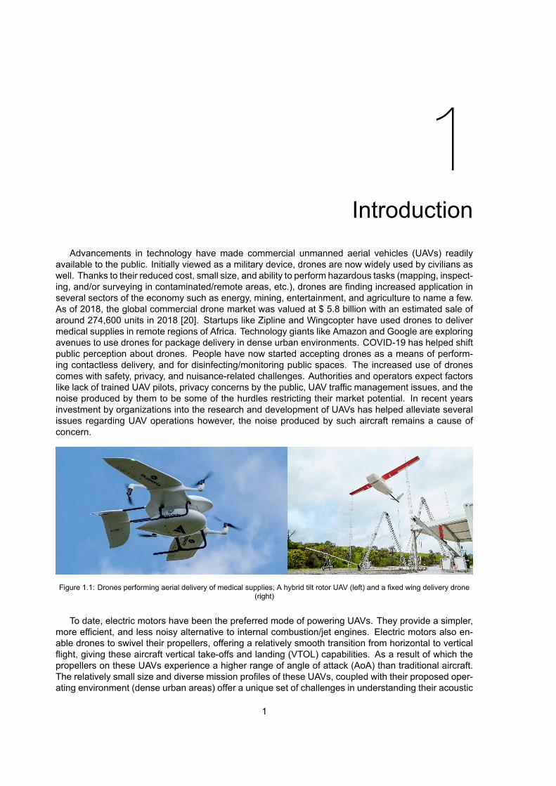
Advancements in technology have made commercial unmanned aerial vehicles (UAVs) readilyavailable to the public. Initially viewed as a military device, drones are now widely used by civilians aswell. Thanks to their reduced cost, small size, and ability to perform hazardous tasks (mapping, inspect-ing, and/or surveying in contaminated/remote areas, etc.), drones are finding increased application inseveral sectors of the economy such as energy, mining, entertainment, and agriculture to name a few.As of 2018, the global commercial drone market was valued at $ 5.8 billion with an estimated sale ofaround 274,600 units in 2018 [20]. Startups like Zipline and Wingcopter have used drones to delivermedical supplies in remote regions of Africa. Technology giants like Amazon and Google are exploringavenues to use drones for package delivery in dense urban environments. COVID-19 has helped shiftpublic perception about drones. People have now started accepting drones as a means of perform-ing contactless delivery, and for disinfecting/monitoring public spaces. The increased use of dronescomes with safety, privacy, and nuisance-related challenges. Authorities and operators expect factorslike lack of trained UAV pilots, privacy concerns by the public, UAV traffic management issues, and thenoise produced by them to be some of the hurdles restricting their market potential. In recent yearsinvestment by organizations into the research and development of UAVs has helped alleviate severalissues regarding UAV operations however, the noise produced by such aircraft remains a cause ofconcern.
Figure 1.1: Drones performing aerial delivery of medical supplies; A hybrid tilt rotor UAV (left) and a fixed wing delivery drone(right)
To date, electric motors have been the preferred mode of powering UAVs. They provide a simpler,more efficient, and less noisy alternative to internal combustion/jet engines. Electric motors also en-able drones to swivel their propellers, offering a relatively smooth transition from horizontal to verticalflight, giving these aircraft vertical take-offs and landing (VTOL) capabilities. As a result of which thepropellers on these UAVs experience a higher range of angle of attack (AoA) than traditional aircraft.The relatively small size and diverse mission profiles of these UAVs, coupled with their proposed oper-ating environment (dense urban areas) offer a unique set of challenges in understanding their acoustic
1

2 1. Introduction
characteristics.Over the years, there have been several successful attempts in understanding and isolating the
noise of propellers operating at high Reynolds numbers (> 10 ). However, research to understandthe aerodynamic and aeroacoustic characteristics of propellers operating at low Reynolds (< 2 ∗ 10 )numbers and with an AoA is limited. The thesis aims to address the research gap by performing acritical analysis on the aerodynamic and aeroacoustic characteristics of propellers operating at lowReynolds numbers with an AoA.
1.1. Research objectiveResearchers have dedicated considerable resources towards understanding the effect of installation
(presence of wings, nacelle, strut, etc.) and small variations in AoA [12, 21–23] on the aerodynamicand acoustic characteristics of propellers. However, most of these analyses were performed in thelate 1900s for large turbo-prop aircraft operating at considerably higher Reynolds numbers (> 10 ).Around 2010, manufacturers like DJI, Parrot, etc., made drones available to commercial consumers.The availability of commercial drones sparked a new wave of research in the field of UAVs. The pastdecade has seen researchers conduct several studies to understand the aerodynamic and acousticcharacteristics of propellers at low Reynolds numbers. These studies, however, havemainly been donefor axisymmetric inflow conditions. Most commercial UAVs (tilt or multi-rotor) have VTOL capabilities. Atypical mission profile of such a UAV includes vertical take-off, landing, transitioning to horizontal flight,and cruise. The propellers experience significant changes in AoA during these flight phases. Thenon-zero AoA results in unsteady loading due to the variation in effective AoA for the propeller bladeelement around the propeller plane. These changes impact the aerodynamics, and consequently, theacoustic characteristics of the propeller. The goal of this thesis is:
“To characterize andquantify the effect of non-axisymmetric inflowconditionson theaerodynamicandacousticpropertiesofpropellersoperatingat lowReynoldsnumbers.”
The goal shall be met by attaining the following objectives:
1. Understanding the aerodynamic and acoustic characteristics of propellers operating at lowReynoldsnumbers and identify the differences compared to propellers operating at high Reynolds numbers.
2. Quantifying and analyzing the changes in aerodynamic and acoustic characteristics of the pro-peller due to AoA.
The first objective is met by carrying out an extensive literature review. The learnings from theliterature reviewed are discussed in Chapter 3. The chapter also lists the research questions that willbe answered through this thesis. The second objective has been achieved by carrying out a high-fidelity computational analysis of a UAV propeller operating at a low Reynolds number. The details ofthe setup used have been discussed in Chapter 5. The following section discusses the approach takento reach the objective and the motivation behind its selection.
1.2. ApproachBased on the literature review and in consideration of the present experimental research at TU
Delft, conducting a computational study was deemed to be the best approach. It would complementthe experimental research and help create a benchmark computational setup that can be used forfuture studies. The computational analysis also provides some distinct advantages over experimentalstudies, which are listed below:
• It eliminates the uncertainties caused due to structural vibrations experienced by an experimentalsetup. Which could translate into unsteady blade motion resulting in additional noise sources.
• Acoustic measurements in a computational analysis do not contain wind tunnel background noiseand other superfluous noise sources, such as electric motor noise, making it easier to analyzethe aerodynamic noise produced by the propeller.

1.3. Outline of thesis 3
• In a computational analysis, placement of microphones does not alter the flow field, enabling a360 directivity analysis.
The computational setup consists of an isolated twin-bladed propeller with a diameter of 30 𝑐𝑚 ro-tating at 6, 000 RPM. The simulation is carried out with a free stream velocity of 12 𝑚/𝑠𝑒𝑐 at an AoAof 0 and 15 . A high fidelity computational flow solver PowerFLOW®, developed by Dassault Sys-tèmes has been utilized for this study. It utilizes the lattice-Boltzmann method (LBM) alongside a verylarge-eddy simulation (VLES) turbulence modeling approach to resolve the flow field. The reason forchoosing such a solver over a traditional Navier-Stokes-based solver is their higher computational effi-ciency, lower dispersion, and dissipation errors [24]. The computation of the acoustic field is performedusing the Ffowcs Williams–Hawkings (FWH) analogy. A more detailed discussion on the flow solverand the computational setup has been carried out in Chapter 4 and 5 respectively.
1.3. Outline of thesisAlong with the present chapter, this report consists of 8 other chapters. A brief introduction to which
has been provided below:
• Chapter 2: provides the reader with the theoretical background in propeller aerodynamics andaeroacosutics .
• Chapter 3: introduces the reader to the flow physics of a propeller operating at an AoA. It alsodiscusses research in this field of propeller performance at low Reynolds numbers.
• Chapter 4: introduces the principles of the LBM, and its implementation into the flow solver.The chapter also discusses the implementation of the FWH analogy in the aeroacoustic solver ofthe tool.
• Chapter 5: presents the setup created to perform the analysis in PowerFLOW®. It includesdescription of the computational geometry, resolution and simulation parameters.
• Chapter 6: discusses the results of the grid resolution study. It also presents the validation ofthe computational data obtained by comparison against experimental data.
• Chapter 7: explains the results, through the analyses of the flow field and post-processing ofacoustic data.
• Chapter 8: provides the conclusion to the thesis and summaries the key results and theirsignificance. It concludes by discussing recommendations for the extension of this study.

2Theoretical Background
This chapter provides the reader with a theoretical background and concepts that shall be usedthroughout the thesis. Section 2.1 introduces the reader to the fundamentals of propeller aerodynam-ics. In Section 2.2 the basic definition of sound, types of sound sources, and sound measurementtechniques are discussed. Section 2.3 discusses the study of noise generated by fluid-solid interac-tion. The chapter ends with a review of acoustic analogies that are used for modeling aerodynamicnoise sources.
2.1. Propeller aerodynamicsLiterature classifies rotating blades into three main categories fans, propellers, and rotors. The
mechanism by which these rotating blades produce thrust is the same. Rotors and fans differ from apropeller in terms of flow regime and number of blades, respectively. A rotor experiences radial inflowacross its disc during a forward flight (similar to a helicopter, see Fig. 2.1a), whereas a propeller expe-rience axial inflow. A propeller and a fan experience axial inflow condition, but fans have a significantlyhigher number of blades (8+) than propellers. It results in much higher wake interaction between theblades.
A propeller is a mechanical device consisting of a rotating shaft with blades attached to it. Theseblades are broad and angled, which help move a vehicle (typically an aircraft or marine vessel). Theblades have the cross-section of an airfoil, and the propeller operates by using the torque generatedby a power source to accelerate a mass of fluid, which produces thrust. Essentially a propeller can bere-imagined as a rotating wing that moves through an air mass by pushing it back and accelerating it,as shown in Fig. 2.1b. The airfoil theory describes how the acceleration of flow over an airfoil resultsin low pressure (suction side at the top) and high pressure (pressure side at the bottom) of the airfoil,producing lift. The airfoil theory, coupled with Newton’s third law can explain how a propeller bladegenerates thrust.
(a) Inflow condition for a rotor disc (b) Propeller blade cross section and velocity diagram [25]
Figure 2.1: Propellers and rotors
4

2.1. Propeller aerodynamics 5
The blades of a propeller rotate about their axis while moving forward. The AoA of a propeller bladeelement is defined as the angle at which the air (relative wind) strikes the propeller blade or the anglebetween relative airflow and the propeller chord line. As a result of this AoA, the air mass flowingover the propeller produces a net aerodynamic force known as the total reaction (TR) force, shownin Fig. 2.2b, which can be broken into its two key components lift (thrust) and drag. With an increasein AoA, lift (thrust in case of propeller) increases linearly (generally up to 15 ± 2 ) and then drops.The drop in lift is due to the stalling of the airfoil. The drag force keeps increasing exponentially withincreasing AoA. Hence for fixed pitch propellers, there is an optimum AoA at which the efficiency isthe highest, while variable pitch, propellers that can adjust blade angle in flight, change blade angledepending on the flight phase, shown in Fig. 2.3. A variable pitch mechanism, because of its weight andmechanical complexity, is not suitable for small UAVs. UAV propeller designers optimize the propellersfor a particular flight phase and AoA, resulting in reduced efficiency for the propellers in off-designconditions.
(a) Uneven loading caused at the propeller disc due to AoA [25]
(b) Forces experienced by a propeller blade element [26]
Figure 2.2: Force experience by a propeller at an AoA
Figure 2.3: Change in Propeller efficiency vs advance ratio at specific blade AoA [2]
During the cruise phase, propellers are at a shallow (or 0 ) AoA resulting in axial inflow conditionand steady disc loading. The new generation of PAVs and UAVs feature electric motors and novel tilt-rotor mechanisms, along with mission profiles that include transitions from vertical to horizontal flightpaths (and vice-versa). These propellers operate at a wide range of AoA and experience non-axialinflow conditions. The non-axial inflow results in the variation of resultant velocity experienced by thepropeller blade at a different azimuthal position (Ψ), resulting in the change of local blade AoA aroundthe propeller plane. As a propeller has a similar operating principle to a wing, changes in AoA result invariation of the net aerodynamic forces experienced by the propeller, resulting in asymmetric loadingof the propeller disc, shown in Fig. 2.2a.

6 2. Theoretical Background
2.2. SoundThis section introduces the reader to the properties and sources of sound and the basics of sound
measurement techniques.
Figure 2.4: Compression and expansion of air due to propagation of sound waves [3]
Sound is a mechanical wave (longitudinal wave) that propagates through a medium (solid, liquid,or gas) in the form of isentropic pressure fluctuation. It creates a region of compression and expansion(high/low pressure) in its direction of propagation, as shown in Fig. 2.4. The rate (per sec) of compres-sion and expansion determines the frequency of a particular sound wave. The audible frequency rangefor humans lies in the frequency band of 20-20,000 𝐻𝑧. The speed (𝑐) at which the fluctuation travelsthrough a medium (ideal gas) is given by:
𝑐 = √𝛾𝑅∗𝑇
mol (2.1)
where 𝛾 is the adiabatic index (1.4 at 0 °C, for air), 𝑅∗ is the universal gas constant (8.314 Jmol 1 K 1),𝑇 is the absolute temperature (K), and mol is the molar mass of the gas. This means that the speedof sound is dependent upon the physical properties of the medium through which it travels, as seen inTable 2.1.
Medium Speed of Sound (𝑚/𝑠𝑒𝑐) Temperature (K)Air 331 273Helium 965 273Air 343 293Fresh Water 1,480 293Lead 1,960 –Glass 5,640 –
Table 2.1: Speed of sound in different mediums [19]
The terms sound and noise are used interchangeably, however, there is a difference between them.Sound can be desirable or undesirable, like the sound produced by a speaker or a passing aircraft.Noise is an unwanted sound, which may cause annoyance or physical discomfort.
2.2.1. Sources of soundSources of sound have diverse sound generation mechanisms, directivity, frequency spectra, and
radiation efficiency. Most sound sources consist of a mixture of elementary source types, which isdependent upon the sound generation mechanism. The three fundamental source types that make upmost of the sound sources are acoustic monopole, dipole, and quadrupole, see Fig. 2.5. This sectionexplains the different characteristics of these elementary sound sources.

2.2. Sound 7
Figure 2.5: Radiation pattern of different sound sources [4]
• Monopole: Amonopole is the building block for all the other elementary sources of noise, such asdipoles and quadrupoles. The dimensions of monopole sources are typically much smaller thanthe radiated sound wavelength. The pressure amplitude radiated by a monopole in the far-fieldis given by:
|𝑝(𝑥, 𝜙, 𝑡)| = 𝑆𝜌𝑐𝑘4𝜋𝑥 (2.2)
where, 𝑘 is the wavenumber given by or , 𝑆 is the source strength, and 𝑥 is the distancebetween the source and the observer.The pressure amplitude for a point source does not depend on the radiation angle (𝜙); hence amonopole radiates sound equally in all directions. The sound power (Π) radiated by a monopolesource is given by [27]:
Π = 𝑆 𝜌𝑐𝑘8𝜋 (2.3)
as 𝑘 = , the above equation can also be written as Π ∼ 𝑓 , meaning that the sound powerradiated by a monopole varies with the square of the frequency.
• Dipole: A dipole is made up of two monopoles of equal strength but opposite phases. Thedistance between the two monopoles in a dipole satisfies 𝑘𝑑 << 1, where 𝑑 is the distancebetween two monopoles. The pressure amplitude of a dipole radiated in the far-field is given as
|𝑝(𝑥, 𝜙, 𝑡)| = 𝑆𝜌𝑐𝑘4𝜋𝑥⏝⎵⏟⎵⏝
Source term
∗𝑘𝑑 ∗ 𝑐𝑜𝑠𝜙⏝⏟⏝Directivity
(2.4)
where 𝑘𝑑 relates the radiated wavelength to the distance between two monopoles.The directivity function depends on 𝜙, meaning that the sound is not radiated equally in all di-rections (max when 𝜙 = 0 and 180 ). The sound power radiated by a dipole varies with the4 power of frequency (Π ∼ 𝑓 ), meaning that a monopole source is more efficient in radiatinglow-frequency sound with similar source strength than a dipole source.
• Quadrupole: A quadrupole source consists of two dipoles of equal strengths but opposite phaseor four monopoles with alternating phase, as seen in Fig. 2.5. The monopoles are separated bya distance of 𝑑 and 𝑑 (horizontal and vertical). The separation is smaller than the wavelengthof the sound produced. The pressure amplitude produced by a quadrupole source in the far-fieldis given by:

8 2. Theoretical Background
|𝑝(𝑥, 𝜙, 𝑡)| = 𝑆𝜌𝑐𝑘4𝜋𝑥⏝⎵⏟⎵⏝
Source term
∗4𝑘 𝑑 𝑑 ∗ 𝑐𝑜𝑠𝜙𝑠𝑖𝑛𝜙⏝⎵⎵⏟⎵⎵⏝Directivity
(2.5)
The directivity is such that there are four angles (𝜙) of high noise radiation and four shadowregions. The sound power radiated by a quadrupole varies with the 6 power of frequency. Fora source of similar strength, a quadrupole is the least efficient radiator for low-frequency noise.
2.2.2. Measurement of soundMeasuring a source of sound helps in quantifying the pressure fluctuation produced by it. Sound
waves with pressure fluctuation in the range of 20𝜇 𝑃𝑎 to 2, 000 𝑃𝑎 fall within the audible band of anaverage human and are of particular interest for most acoustic studies. Given the range of pressurefluctuation, it is difficult to capture it on a linear scale against a standard atmospheric pressure of101, 325 𝑃𝑎. Hence, a logarithm scale (decibel 𝑑𝐵) is used to measure sound, and the most commonquantity used to describe it is sound pressure level (SPL). It is defined as:
𝑆𝑃𝐿 = 10 ∗ 𝑙𝑜𝑔 (𝑝𝑝 ) (2.6)
where 𝑝 is the root mean square of the pressure fluctuation and 𝑝 is the reference pressure. Itis 2 × 10 𝑃𝑎 for air and is the minimum threshold of human hearing, as shown in Fig. 2.6.
Figure 2.6: Effective Sound pressure and corresponding SPL in decibel scale [5]
A sound signal consists of multiple frequencies. Human ears, similar to human eyes, are more sen-sitive to a specific range of frequency. The International Electro-Technical Commission (IEC) definesa family of curves that provide an independent standardized way of measuring sound perceived byhumans, see Fig. 2.7. It applies a certain weight to the measured SPL as per their frequency and isdefined under IEC 61672:2003 as:
• A - weighting is most commonly used for measuring environmental and industrial noise, as well asin the assessment of potential hearing damage and other noise health effect at all sound levels.
• B, D - weightings are no longer described in IEC 61672:2003, but their frequency response canbe found in older IEC 60651. It is interesting to note that D-frequency-weighting was developedspecifically for high-level aircraft noise under the IEC 537 measurement standard.
• C - weighting is in use by many sound level meters, and their fitting is mandated (at least fortesting purpose) to precision (class one) sound level meters.
Applying Fourier transform converts a pressure signal in the time domain to acoustic spectra inthe frequency domain. A noise spectrum represents the contribution of different frequencies to theoverall sound pressure level (OASPL). OASPL is used to quantify the total energy contained in a noisespectrum. Performing a Fourier transform on a pressure signal reveals its characteristics (tonal or

2.3. Aeroacoustics 9
Figure 2.7: Weighting graph for sound pressure levels [6]
broadband) and helps detect its dominant features. Tonal noise can be defined as a discrete frequencynoise characterized by spectral peaks at specific frequencies, as shown in Fig. 2.8. Broadband noise,also know as wideband noise, is a noise whose energy is distributed over a wide range of frequencieswith no distinct peaks in the spectrum.
Figure 2.8: Converting pressure signal from a propeller analysis to power spectrum
2.3. AeroacousticsAeroacoustic is a discipline that combines fluid mechanics with classical acoustics to study the noise
produced by an aerodynamic source. It analyses and quantifies noise generated due to unsteady fluidmotion and interaction of surfaces with fluid in motion, resulting in fluctuating aerodynamic forces. Thecharacteristics of noise generated by a propeller are discussed in Section 2.3.1 and the broadbandnoise generation mechanism of an airfoil is discussed in Section 2.3.2.
2.3.1. Propeller noiseNoise has been one of the main factors limiting the widespread use of propeller-driven aircraft.
This section introduces the reader to the characteristics of noise generated by a propeller and brieflyexplains the mechanism behind them.
Propeller noise is classified into tonal noise and broadband noise, see Fig. 2.8. Pressure fluctua-tions produced by the rotation of a propeller blade in a fluid medium consist of tonal and broadbandcomponents. Fig. 2.9 shows the pressure fluctuation produced by a three-bladed propeller in one rota-tion. The top left corner of the figure represents the tonal component of the pressure signal. The threedistinct pressure peaks observed in the signal repeat themselves per rotation and are responsible for
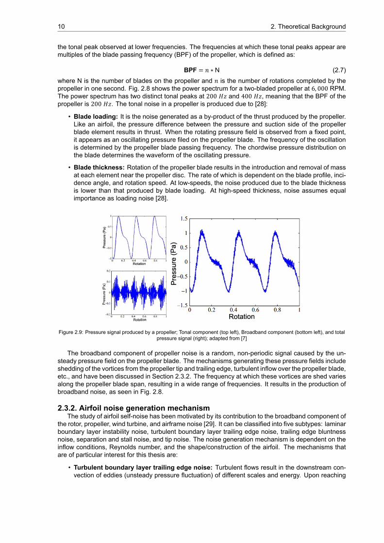
10 2. Theoretical Background
the tonal peak observed at lower frequencies. The frequencies at which these tonal peaks appear aremultiples of the blade passing frequency (BPF) of the propeller, which is defined as:
BPF = 𝑛 ∗ N (2.7)where N is the number of blades on the propeller and 𝑛 is the number of rotations completed by thepropeller in one second. Fig. 2.8 shows the power spectrum for a two-bladed propeller at 6, 000 RPM.The power spectrum has two distinct tonal peaks at 200 𝐻𝑧 and 400 𝐻𝑧, meaning that the BPF of thepropeller is 200 𝐻𝑧. The tonal noise in a propeller is produced due to [28]:
• Blade loading: It is the noise generated as a by-product of the thrust produced by the propeller.Like an airfoil, the pressure difference between the pressure and suction side of the propellerblade element results in thrust. When the rotating pressure field is observed from a fixed point,it appears as an oscillating pressure filed on the propeller blade. The frequency of the oscillationis determined by the propeller blade passing frequency. The chordwise pressure distribution onthe blade determines the waveform of the oscillating pressure.
• Blade thickness: Rotation of the propeller blade results in the introduction and removal of massat each element near the propeller disc. The rate of which is dependent on the blade profile, inci-dence angle, and rotation speed. At low-speeds, the noise produced due to the blade thicknessis lower than that produced by blade loading. At high-speed thickness, noise assumes equalimportance as loading noise [28].
Figure 2.9: Pressure signal produced by a propeller; Tonal component (top left), Broadband component (bottom left), and totalpressure signal (right); adapted from [7]
The broadband component of propeller noise is a random, non-periodic signal caused by the un-steady pressure field on the propeller blade. The mechanisms generating these pressure fields includeshedding of the vortices from the propeller tip and trailing edge, turbulent inflow over the propeller blade,etc., and have been discussed in Section 2.3.2. The frequency at which these vortices are shed variesalong the propeller blade span, resulting in a wide range of frequencies. It results in the production ofbroadband noise, as seen in Fig. 2.8.
2.3.2. Airfoil noise generation mechanismThe study of airfoil self-noise has been motivated by its contribution to the broadband component of
the rotor, propeller, wind turbine, and airframe noise [29]. It can be classified into five subtypes: laminarboundary layer instability noise, turbulent boundary layer trailing edge noise, trailing edge bluntnessnoise, separation and stall noise, and tip noise. The noise generation mechanism is dependent on theinflow conditions, Reynolds number, and the shape/construction of the airfoil. The mechanisms thatare of particular interest for this thesis are:
• Turbulent boundary layer trailing edge noise: Turbulent flows result in the downstream con-vection of eddies (unsteady pressure fluctuation) of different scales and energy. Upon reaching

2.4. Aeroacoustic analogies 11
the trailing edge of an airfoil, these eddies experience a sudden change in pressure and acousticimpedance and scatter as broadband noise. It is a significant contributor to the noise producedby propellers and wind turbines [30].
Figure 2.10: Turbulent boundary layer trailing edge noise [8]
• Separation and stall noise: At high AoA, depending on Reynolds number and airfoil character-istics, flow separation may occur on the suction side of the airfoil. Flow separation at the suctionside results in unsteady flow and generation of tonal humps in the broadband spectrum due tovortex shedding [31]. It can be avoided by tripping the propeller blades [32].
Figure 2.11: Separation and stall noise [8]
2.4. Aeroacoustic analogiesAn acoustic analogy reduces the source of aeroacoustic noise into simple emitter types and de-
couples the noise generation mechanism from its pure propagation. It is achieved by rearranging theequations governing the acoustic field such that the field variables (wave operator) are on the left-hand side of the equation and the source quantities to the acoustic field (source part) on the right-handside. Doing so enables the use of CFD/CAA simulations to computationally predict noise in the far-field without the need for a large simulation domain with high resolution. The three most commonlyused acoustics analogies were developed by Lighthill, an extension to Lighthill’s analogy by Curle, andFfowcs Williams & Hawkings. Sections 2.4.1 and 2.4.2 explains the characteristics of these analogiesand their relevance for the present study, however, before expanding on the analogies the sectiondiscusses the basic equations defining linearised acoustic wave propagation and generation.
Consider a medium with a stationary flow such that the average flow properties are uniform through-out the flow domain. As an acoustic wave propagates through the medium, it becomes the only sourceof pressure and velocity fluctuation. For a sound wave traveling isentropically through the medium, therelation between pressure and density perturbation is given as:
𝑝 = 𝜌 𝑐 where 𝑐 = (𝜕𝑝𝜕𝜌) (2.8)
By assuming that the acoustic wave results in small density perturbation (𝜌 ) in the medium, 𝜌 <<𝜌 where 𝜌 is the mean density, substituting it in the continuity equation gives:
𝜕𝜌𝜕𝑡 + 𝜌
𝜕𝑣𝜕𝑥 ≈ 0 (2.9)
where 𝑣 is the velocity fluctuation induced by the acoustic wave.Next, the momentum equation is modified by neglecting the effects of viscosity and applying a
small perturbation assumption to it. The small perturbation assumption helps linearise the equation byignoring all second-order terms, resulting in:

12 2. Theoretical Background
𝜌 𝜕𝑣𝜕𝑡 +
𝜕𝑝𝜕𝑥 ≈ 0 (2.10)
By combing the momentum and continuity equation, the linear homogeneous acoustic wave equa-tion is obtained. It forms the base for all calculation in the field of linear acoustics and is given as[7]:
1𝑐𝜕 𝑝𝜕𝑡 − ∇ 𝑝 = 0 (2.11)
where 𝑝 is the pressure fluctuations caused by the acoustic wave. In the linear homogeneous acousticwave equation, the effect of external force (𝐹), mass, and momentum injection are neglected, and thefluid domain is assumed to be stationary. It can not be used to describe an acoustic wave propagatingfrom a source of sound or in a non-stationary medium.
A wave equation that includes the sound source is defined using an inhomogeneous wave equation.It is derived by rearranging the momentum and continuity equations. The process is similar to derivingthe linearised homogeneous wave equation without neglecting the effect of external force (𝐹), mass,and momentum injection. Which results in [33]:
1𝑐𝜕 𝑝𝜕𝑡 − ∇ 𝑝 = 𝜕𝑚
𝜕𝑡⏟Monopole
− ∇.𝐹⏟Dipole
(2.12)
Eq. (2.11) and Eq. (2.12) are similar to each other, except for the monopole and dipole source termson the right-hand side of the equation.
Monopole: A monopole source term represents the displacement of mass ( ) in the system. Asdescribed in Section 2.2.1, such a source radiates noise equally in all directions. The sound producedby the displacement of air by a propeller is a monopole sound source.
Dipole: A dipole source represents the noise produced by the force exerted on the flow. The forcesexerted by rotating propellers into the flow are an example of such a source.
2.4.1. Lighthill’s acoustic analogyLighthill’s acoustic analogy provides the theory for the sound generated by turbulence and helps in
identifying the source of sound in an arbitrary unsteady flow [7]. Based on exact equations of fluid flow,Lighthill’s equations make no assumptions relating to compressibility effects and is given as [34, 35]:
𝜕 𝜌𝜕𝑡 − 𝑐 𝜕 𝜌𝜕𝑥 =
𝜕 𝑇𝜕𝑥 𝜕𝑥 (2.13)
Where 𝑇 is the Lighthill’s stress tensor and is given by:
𝑇 = 𝜌𝑢 𝑢 + (𝑝 − 𝑐 𝜌)𝛿 − 𝜏 (2.14)
The LHS of the equation describes the acoustic wave propagation in a uniform medium, where𝜌 = ( ) is the dependent variable and 𝑐 is the speed of sound in the stationary medium. The RHSdescribes the source term consisting of all the effects that generate the wave. The Lighthill’s stresstensor 𝑇 in is defined as:
• 𝜌𝑢 𝑢 : is the Reynolds stress tensor.
• (𝑝 − 𝑐 𝜌)𝛿 : represents the excess momentum transfer by pressure and can be ignored in anisothermal, incompressible flow [36].
• 𝜏 : is the viscous stress tensor and can be ignored for high Reynolds number flow.
A closer analysis of the source term reveals a second-order spatial derivative, making it a quadrupolesource of the sound [37]. It also means that the source term only models free turbulence and does notaccount for the effect of moving boundaries or surfaces present in the flow. The presence of a sur-face/solid body in the flow influences how sound waves are produced and radiated in the sound field.

2.4. Aeroacoustic analogies 13
Not being able to account for the presence of a surface was a limitation of Lighthill’s analogy. Curle [38]in 1955 extended Lighthill’s analogy to include the effects of a surface/solid body in the flow. Curle’sanalogy is relatively advanced to Lighthill’s analogy, however, it assumes the surface to be stationary inthe fluid. The noise produced by propellers is due to moving surfaces, as result, both these analogiesare unsuitable for analyzing the acoustic field of rotating propellers.
2.4.2. Ffowcs-Williams and Hawkings (FWH) analogyFWH [39] extended Lighthill’s and Curle’s analogy in 1969 to include moving surfaces. It redefines
the pressure, density, and velocity variables in terms of generalized derivatives such as the Heavisidestep function 𝐻 and substitutes these variables into the continuity and momentum equations. Theequations are solved to obtain a wave equation in terms of the new variables. It is the FWH equation,given as:
𝜌 (𝑥, 𝑡)𝑐 𝐻 = 𝜕𝜕𝑥 𝜕𝑥 ∫ [
𝑇4𝜋𝑟 |1 − 𝑀 |] ∗
𝑑𝑉(𝑧)
− 𝜕𝜕𝑥 ∫ [
(𝜌𝑣 (𝑣 − 𝑉 ) + 𝑝 ) 𝑛4𝜋𝑟 |1 − 𝑀 | ]
∗𝑑𝑆
+ 𝜕𝜕𝑡 ∫ [
(𝜌𝑣 − 𝜌 𝑉 ) 𝑛4𝜋𝑟 |1 − 𝑀 | ] ∗
𝑑𝑆
(2.15)
The modification makes the FWH analogy suitable for performing analysis for propeller noise. The
( ) term physically signifies the impact of motion of the source on its time history. The significanceof the other terms on the RHS are as follows [7]:
• Quadrupole term: it is defined as the volume source term and its strength depends upon 𝑇 . Itconsists of sound radiated by turbulence and flows distortion due to shock waves. At low speeds,this term is of negligible importance.
• Dipole term: It is the second term of the equation and is controlled by surface loading 𝑝 .
• Monopole term: It is a volume displacement source and is dependent upon the blade surfacevelocity and the density at the observer.
FWH analogy can model noise produced by moving sources, making it the most suitable analogyfor modeling propeller noise. PowerFLOW® uses the FWH analogy for computing the aeroacousticproperties. The way an FWH analogy works in a CAA setup is [40]:
1. The acoustic pressure fluctuations produced by the source are captured inside a control surfaceusing a fine mesh. It is done by placing permeable or solid integrating surfaces in the controlvolume, details of which have been discussed in Section 4.3.1.
2. The acoustic reciprocity theorem is then used to collect and find equivalent sources (monopoles,dipoles, and quadrupoles) to set at the control surface.
3. Linear acoustic propagation schemes are then used to calculate the noise in the far-field.

3Literature Review
This chapter reviews the research done in the field of propeller aerodynamics and aeroacoustics.Part one, Section 3.1, of this chapter recapitulates the research done on propellers operating at highReynolds numbers (𝑅𝑒) and the impact of inflow angle on their characteristics. It is achieved by dis-cussing the various experimental, analytical, and numerical techniques used to analyze propeller char-acteristics. Part two, Section 3.2, of this chapter, reviews the most recent research on propellers oper-ating at low Reynolds number. The section is divided into an aerodynamic and an acoustics section.They address the progress made in the field and identify the research gaps. The final part, Section 3.3,of this chapter, presents the research question that the author aims to answer through this thesis.
3.1. Fundamental researchPropellers preceded all means of powering an aircraft by several decades and saw significant im-
provement in their performance between the 1930s & 40s. It was during this period Gutin [41] startedperforming theoretical work in understanding the sound field produced by a rotating propeller. Theintroduction of jet engines in the 1950s saw the propellers fall out of favor for a less efficient thoughfaster means of propulsion, causing a slump in propeller-related research. In the 1970s, however, asteep rise in fuel cost shifted the attention back to efficiency spurring propeller-related research.
Researchers were concerned about the increase in annoyance due to low flying aircraft poweredby propellers. The projected rise in the use of such aircraft was a big motivation to develop noiseabatement techniques. By 1970, analytical studies recognized blade thickness and loading, tip vortex,and trailing edge vortex as the primary sources of aerodynamic noise on a propeller. Researchers wereable to identify that factors such as the number of blades, flow velocity, flow direction play a vital rolein determining the acoustic characteristics of a propeller [28]. Quantification, detailed analysis, andvalidation of these theoretical results were limited by the experimental and computational resourcesavailable at the time.
Post-1970s the renewed interest in propeller-powered aircraft lead to the development of advancedturboprops and prop fans. These developments were supported by advancements in experimental andcomputational research, enabling researchers to validate the analytical models and explain propellernoise radiation and generation mechanism. One such model is the helicoidal surface theory developedby Hanson [42] in 1980. The analytical model used a frequency domain analysis of the pressure field toshow how blade thickness, chord length, sweep, and the airfoil section shape influenced noise radiation.The theoretical results were compared against experimental data from a supersonic tip speed propellerat a flight Mach number of 0.32 and showed good agreement. The model assumed the propeller to bein a uniform axial inflow condition. However, it paved the way for future research in non-axial inflowconditions by providing a way to account for variation in blade geometry on far-filed noise.
In the mid-1980s, the International Civil Aviation Organization (ICAO) introduced a new procedurein the noise certification of propeller-driven aircraft. The new regulations required the aircraft noise tobe measured during the cruise, take-off, and approach flight phase. The propeller operates at an AoAduring take-off and approach conditions. The non-axial inflow conditions result in the variation of aero-dynamic as well as acoustic characteristics of the propeller. The fundamental cause and mechanisms
14

3.1. Fundamental research 15
of which have been discussed in the following sections.
3.1.1. Radial directivityOperating under non-axial inflow propeller blade experiences periodic variation in the magnitude
of inflow velocity and local blade AoA. The accompanying variation in the helical propeller tip Machnumber (𝑀 ) and its AoA (𝛼 ), wrt. to 0 AoA, can be expressed as a function of its azimuthal angle(Ψ), advance ratio (𝐽), and propeller disc AoA (𝛼), and is given as [9]:
𝑀 (𝛼,Ψ)𝑀 (𝛼 = 0) = √1 +
2𝐽 sin𝛼 sinΨ1 + 𝐽 (3.1)
Δ𝛼 = 𝑡𝑎𝑛 [𝐽(1 − cos𝛼 + 𝐽 sin𝛼 sinΨ)1 + 𝐽 cos𝛼 + 𝐽 sin𝛼 sinΨ] (3.2)
(a) Side view of propeller microphone setup (b) Front view of propeller microphone setup
Figure 3.1: Visualisation of propeller disc AoA; adapted from [9]
Based on Eq. (3.1) and Eq. (3.2), it can be seen that the maximum value wrt. 0 AoA will beattained when Ψ = 90 (or 270 depending on how AoA and Ψ are defined). Experiments performedby Dobrzynski et al. [9] found that for a microphone in the propeller plane the pressure amplitude isgoverned by the pressure wave being produced by the propeller blade advancing in the direction ofthe microphone. From theoretical knowledge, it is deduced that the variation in the helical tip Machnumber (𝑀 ) and local AoA (𝛼 ) will result in variation of the pressure amplitude produced by thepropeller blade. The variation in pressure amplitude will cause a change in the SPL calculated at themicrophone location and produce asymmetry in circumferential noise directivity.
(a) Variation in local AoA ( ) (b) Variation in helical tip Mach number
Figure 3.2: Variation in propeller blade properties with AoA ( ) at
Fig. 3.2 graphically represents the variation in 𝛼 and𝑀 with AoA for different advancing ratio (𝐽).It can be seen that 𝐽 of the propeller has a significant impact on Δ𝛼 , doubling the advanced ratio from
16 3. Literature Review
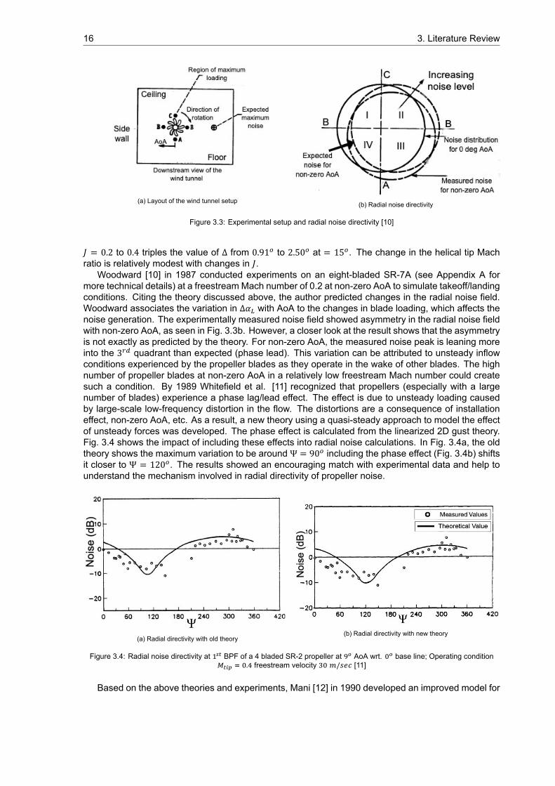
(a) Layout of the wind tunnel setup (b) Radial noise directivity
Figure 3.3: Experimental setup and radial noise directivity [10]
𝐽 = 0.2 to 0.4 triples the value of Δ from 0.91 to 2.50 at = 15 . The change in the helical tip Machratio is relatively modest with changes in 𝐽.
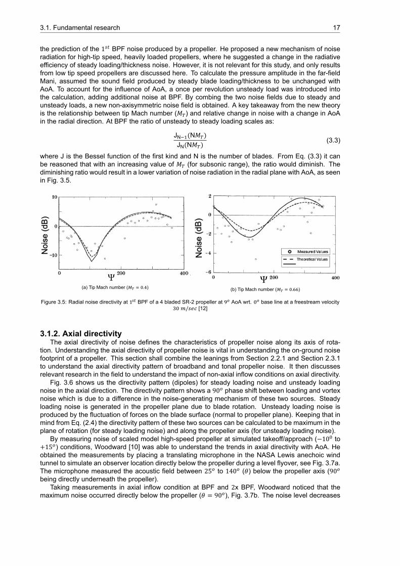
Woodward [10] in 1987 conducted experiments on an eight-bladed SR-7A (see Appendix A formore technical details) at a freestream Mach number of 0.2 at non-zero AoA to simulate takeoff/landingconditions. Citing the theory discussed above, the author predicted changes in the radial noise field.Woodward associates the variation in Δ𝛼 with AoA to the changes in blade loading, which affects thenoise generation. The experimentally measured noise field showed asymmetry in the radial noise fieldwith non-zero AoA, as seen in Fig. 3.3b. However, a closer look at the result shows that the asymmetryis not exactly as predicted by the theory. For non-zero AoA, the measured noise peak is leaning moreinto the 3 quadrant than expected (phase lead). This variation can be attributed to unsteady inflowconditions experienced by the propeller blades as they operate in the wake of other blades. The highnumber of propeller blades at non-zero AoA in a relatively low freestream Mach number could createsuch a condition. By 1989 Whitefield et al. [11] recognized that propellers (especially with a largenumber of blades) experience a phase lag/lead effect. The effect is due to unsteady loading causedby large-scale low-frequency distortion in the flow. The distortions are a consequence of installationeffect, non-zero AoA, etc. As a result, a new theory using a quasi-steady approach to model the effectof unsteady forces was developed. The phase effect is calculated from the linearized 2D gust theory.Fig. 3.4 shows the impact of including these effects into radial noise calculations. In Fig. 3.4a, the oldtheory shows the maximum variation to be around Ψ = 90 including the phase effect (Fig. 3.4b) shiftsit closer to Ψ = 120 . The results showed an encouraging match with experimental data and help tounderstand the mechanism involved in radial directivity of propeller noise.
(a) Radial directivity with old theory(b) Radial directivity with new theory
Figure 3.4: Radial noise directivity at BPF of a 4 bladed SR-2 propeller at AoA wrt. base line; Operating condition. freestream velocity / [11]
Based on the above theories and experiments, Mani [12] in 1990 developed an improved model for
3.1. Fundamental research 17
the prediction of the 1 BPF noise produced by a propeller. He proposed a new mechanism of noiseradiation for high-tip speed, heavily loaded propellers, where he suggested a change in the radiativeefficiency of steady loading/thickness noise. However, it is not relevant for this study, and only resultsfrom low tip speed propellers are discussed here. To calculate the pressure amplitude in the far-fieldMani, assumed the sound field produced by steady blade loading/thickness to be unchanged withAoA. To account for the influence of AoA, a once per revolution unsteady load was introduced intothe calculation, adding additional noise at BPF. By combing the two noise fields due to steady andunsteady loads, a new non-axisymmetric noise field is obtained. A key takeaway from the new theoryis the relationship between tip Mach number (𝑀 ) and relative change in noise with a change in AoAin the radial direction. At BPF the ratio of unsteady to steady loading scales as:
JN (N𝑀 )JN(N𝑀 ) (3.3)
where J is the Bessel function of the first kind and N is the number of blades. From Eq. (3.3) it canbe reasoned that with an increasing value of 𝑀 (for subsonic range), the ratio would diminish. Thediminishing ratio would result in a lower variation of noise radiation in the radial plane with AoA, as seenin Fig. 3.5.
(a) Tip Mach number ( . ) (b) Tip Mach number ( . )
Figure 3.5: Radial noise directivity at BPF of a 4 bladed SR-2 propeller at AoA wrt. base line at a freestream velocity/ [12]
3.1.2. Axial directivityThe axial directivity of noise defines the characteristics of propeller noise along its axis of rota-
tion. Understanding the axial directivity of propeller noise is vital in understanding the on-ground noisefootprint of a propeller. This section shall combine the leanings from Section 2.2.1 and Section 2.3.1to understand the axial directivity pattern of broadband and tonal propeller noise. It then discussesrelevant research in the field to understand the impact of non-axial inflow conditions on axial directivity.
Fig. 3.6 shows us the directivity pattern (dipoles) for steady loading noise and unsteady loadingnoise in the axial direction. The directivity pattern shows a 90 phase shift between loading and vortexnoise which is due to a difference in the noise-generating mechanism of these two sources. Steadyloading noise is generated in the propeller plane due to blade rotation. Unsteady loading noise isproduced by the fluctuation of forces on the blade surface (normal to propeller plane). Keeping that inmind from Eq. (2.4) the directivity pattern of these two sources can be calculated to be maximum in theplane of rotation (for steady loading noise) and along the propeller axis (for unsteady loading noise).
By measuring noise of scaled model high-speed propeller at simulated takeoff/approach (−10 to+15 ) conditions, Woodward [10] was able to understand the trends in axial directivity with AoA. Heobtained the measurements by placing a translating microphone in the NASA Lewis anechoic windtunnel to simulate an observer location directly below the propeller during a level flyover, see Fig. 3.7a.The microphone measured the acoustic field between 25 to 140 (𝜃) below the propeller axis (90being directly underneath the propeller).
Taking measurements in axial inflow condition at BPF and 2x BPF, Woodward noticed that themaximum noise occurred directly below the propeller (𝜃 = 90 ), Fig. 3.7b. The noise level decreases

18 3. Literature Review
(a) Directivity pattern of steady loading noise on thepropeller plane
(b) Directivity pattern of unsteady loading on the propellerplane
Figure 3.6: Propeller noise directivity pattern for axial inflow condition
on both sides of (𝜃 = 90 ). The side lobes occur due to reflection from the tunnel wall and interferencefrom the microphone array. These side lobes are not indicative of the axial directivity of propellernoise. The experimental results, therefore, show the same directivity trends as the theory discussedabove. Measurements with changing AoA showed that the noise levels increase below the propellerwith positive AoA, see Fig. 3.8. The difference in noise levels can be as high as 10 𝑑𝐵 directly belowthe propeller when the AoA changes from 0 to 15 .
(a) Top view of the experimental setup [10] (b) Axial Directivity at AoA
Figure 3.7: Experimental setup and propeller noise directivity at AoA [10]
Figure 3.8: Effect of AoA on axial directivity of BPF [10]
Padula [43] in 1985, conducted further experimental research on the variation in axial directivitywith AoA. He conducted experiments on high (𝑀 = 0.76) and low (𝑀 = 0.4) tip speed propellers at

3.2. Low Reynolds number 19
AoA (±10 ). He found that due to the domination of thickness noise at higher 𝑀 the propellers showrelatively smaller variation in axial directivity with AoA. A similar observation made by Mani [12] hasalso been discussed in Section 3.1.1.
These observations show the variation in acoustic characteristics with AoA and highlight the needfor detailed acoustic analysis of low-speed propellers operating at an AoA. During the 1980s, the focuswas on large propellers operating at high Reynolds numbers for commercial aircraft. It was not untilthe mid to late 2000s that propellers operating at low Reynolds numbers would get their due.
3.2. Low Reynolds numberThis section discusses the most recent research in the field of UAV propellers operating at low
Reynolds numbers. It is divided, into an aerodynamic (Section 3.2.1) and an aeroacoustics (Sec-tion 3.2.2) section. The aerodynamic section explores the variation in aerodynamic characteristics ofairfoils with Reynolds number and its impact on propeller performance. In the aeroacoustics section,the acoustic characteristics of UAV propellers in different configurations are discussed.
3.2.1. Aerodynamic researchA common feature across all commercial UAVs is their compact size and relatively low flight speed,
which effectively translates into an operational Reynolds number of ≤ 2 ∗ 10 . At such low Reynoldsnumbers, viscous forces assume greater importance than the inertial forces within the fluid. It resultsin the change of boundary layer (BL) characteristics, such as flow transition, separation, etc. Fig. 3.9aprovides an insight into these changes with change in Reynolds number. For airfoils operating between10 < 𝑅𝑒 < 5∗10 the BL is stable (due to the influence of viscous forces), and the flow remains laminar(does not separate) for most of the chord length. Due to the relatively low Reynolds number, there isno formation of a turbulent boundary layer over the airfoil resulting in direct flow separation. The flowseparation point starts moving towards the leading edge of the airfoil with an increase in AoA, whichcauses abrupt changes in lift and drag values. At Reynolds number in the range of 5∗10 < 𝑅𝑒 < 2∗10 ,after separation the laminar boundary layer gains enough momentum to reattach itself to the airfoil.The region between the point of separation and reattachment is known as a laminar separation bubble(that spans 15 − 40% of the chord length [44]) and results in increased drag over the airfoil. Thepoint of reattachment is dependent upon the Reynolds number, as a result, the reattachment point isfurther downstream as compared to 𝑅𝑒 > 2 ∗ 10 . Airfoils operating at 𝑅𝑒 > 2 ∗ 10 experience flowtransition (from laminar to turbulent) before flow separation. The turbulent boundary layer energizedby the free stream remains attached to the airfoil and prevents flow separation, improving (𝐶 /𝐶 )performance. As a result of which Reynolds number has a significant impact on airfoil performance,see Fig. 3.9b.
(a) Airfoil boundary layer flow characteristics with [45] (b) Effect of on airfoil sectional ( / ) ; adapted from [44]
Figure 3.9: Impact of on airfoil characteristics
Historically extensive studies have been carried out to understand the performance of propellersoperating at high Reynolds numbers. The efficiency of these fixed pitch propellers peaked (for designedconditions) at around 83% for traditional wooden propellers and went up to 90% for modern compositepropellers [46]. UAV propellers have shown considerably lower performance, with peak efficiency ataround 60 − 70% [47]. These propellers also exhibit a high sensitivity to change in Reynolds number,

20 3. Literature Review
with peak efficiency dropping by 10% as the Reynolds number changes from 2 ∗ 10 to 1 ∗ 10 [47].However, above 𝑅𝑒 = 2 ∗ 10 Reynolds number has a relatively lower impact on propeller efficiency.An experimental study by Gamble showed that efficiency drops by only 5% as the Reynolds numberdrops from 1.1∗10 to 4∗10 [46]. It is due to the variation of (𝐶 /𝐶 ) value with Reynolds number.At 5 ∗ 10 < 𝑅𝑒 < 2 ∗ 10 the (𝐶 /𝐶 ) shows a sharp increase in value resulting in improvedairfoil performance. The improvement in airfoil performance results in better propeller efficiency, as thepropeller can produce more lift (thrust) at lower drag (torque). Experiments by Gamble et al. [46, 47]showed a dependency of propeller performance on Reynolds number and recommended more studiesto quantify the variation. It eventually leads to the development of the UIUC [48] database for lowReynolds number propellers. The database contains performance data of about 79 propellers in the 9to 11-inch diameter range. To examine the Reynolds number effect (𝑅𝑒 range of 5 ∗ 10 − 10 ) thesepropellers were tested for a range of RPM (1, 500 − 7, 500) and echoed the observations made byprevious researchers. The peak efficiency was measure at 65% and went as low as 28% for someReynolds number, and propeller types [49]. The low Reynolds number provides unique challenges inpredicting propeller performance using existing models [50]. As a result, such experiments provide datato validate and improve existing models. A similar approach is taken to understand the impact of inflowangle on propeller performance [51]. A common trend observed is that the thrust value increases withan increase in AoA. The AoA has a comparatively smaller impact on the torque (and consequently thepower consumed) of the propeller [52]. Demonstrating an increase in propulsive efficiency with AoA,however, the difference in propulsive efficiency with AoA collapse when calculated using the inflow-based advance ratio (see Appendix A) [53].
(a) Variation in efficiency of a Zinger 16x6 propeller [47] (b) Variation in efficiency of an APC 18x12 propeller [46]
Figure 3.10: Impact of on airfoil characteristics
3.2.2. Aeroacoustic researchHistorically research on UAVs was primarily geared towards flight dynamics and controls. It helped
understand their performance characteristics but was not much help in improving them. The surgein commercial UAVs use highlighted their performance shortcomings and annoyance caused by theiracoustic signature [13]. According to the literature surveyed [13, 54], the primary sources of propellernoise are steady loading, unsteady loading/vortex sound, and motor noise. The present section willlook into the influence of these sources on the acoustic characteristics of UAV propellers and theirvariation with change in inflow/surrounding condition.
Zawodny et al. [13] conducted acoustic measurements on two isolated propellers (DJI 9443 andAPC 11x4.7 SF) to understand their acoustic characteristics. Measurements were taken by a fivemicrophone arc placed at a distance of 1.9 𝑚 (from the center of the propeller) along the propeller axis.The propellers produced the same thrust at different RPM resulting in a difference of up to 8 𝑑𝐵 in theOASPL. The difference was primarily due to the change in BPF due to RPM. However, on applyingA-weighting to OASPL, the noise advantage from having a lower RPM reduced to less than 3 𝑑𝐵. Thepresence of motor noise in the mid-frequency range (1, 000−3, 000 𝐻𝑧), see Fig. 3.11, can be identifiedas one of the probable causes.
In traditional propellers installation effects, caused due to flow distortions, impact propeller noise [9].Hence, it is imperative to understand the impact of the rotor and airframe interaction on UAV noise to

3.2. Low Reynolds number 21
(a) APC × propeller (b) DJI 9443 propeller
Figure 3.11: Power spectrum plot for at constant thrust of . N [13].
develop amore realistic understanding of their acoustic signature. Zawodny et al. [14] built on the studyof isolated propellers to include UAV airframe, see Fig. 3.12a. The study revealed that the presence ofan airframe close to the rotor (Δ/𝑅 = 0.1) increases the amplitude of BPF harmonics (up to 7 BPF),see Fig. 3.12b. The sudden change in local induced velocity due to the airframe causes unsteady bladeloading, which increases the amplitude of higher harmonics. The rise in amplitude of higher harmonicsfalls significantly with increasing rotor-airframe separation. It starts to resemble the acoustic spectraof an isolated propeller at Δ/𝑅 = 0.5. Yoon, Wang et al. [55, 56] conducted further computational andexperimental studies to understand the impact of rotor mounting location (over vs. under mount) onnoise. The results showed a significantly higher tonal content for under-mounted rotors (especially athigher BPF). The presence of an airframe above the rotor produces large disturbances in the flow field,which results in a larger fluctuation of induced velocity, causing a rise in the amplitude of fluctuatingpressure. It results in the production of higher unsteady noise. These findings are in line with the resultsby Zawodny, Coffen et. al. [14, 57]. The results reported take us a step closer to understanding theacoustic characteristics of UAVs.
(a) Experimental setup used by Zawodny (over mountedrotor configuration)
(b) Impact of rotor airframe separation ( / ) on propeller noise
Figure 3.12: Experimental setup and impact of rotor airframe separation on propeller noise [14]
Yang et al. [15], investigated the impact of freestream velocity and AoA on an isolated UAV rotor.It is the only study (to the best of the author’s knowledge) exploring the effect of shaft AoA on isolatedUAV rotors. The experiment was conducted at an AoA of 90 to 70 , reference AoA defined in Fig. 5.4,for different freestream velocities, and RPM. The increase in freestream velocity at constant RPM andAoA increased the mean thrust produced by a rotor. Operating at an AoA, the radial (𝑐𝑜𝑠) componentof the free stream is responsible for introducing asymmetry in rotor disc loading, see Fig. 3.13. Con-sequently, at fixed free stream velocity, increasing the AoA results in the higher harmonics of the BPF,see Fig. 3.14b. Increasing the free stream velocity at fixed AoA also has a similar effect Fig. 3.14a.The direction of flow over the rotor causes BVI, which could also be one of the probable causes forthe rise in higher harmonics (up to 7 BPF) [15]. The circumferential directivity was measured usingan array of 18 microphones placed at the base of the setup, see Fig. 3.13. The directivity pattern was

22 3. Literature Review
dominated by the 1 BPF noise and is higher in the first and the third quadrants for all AoAs and freestream velocity. Doppler shift, BVI, and higher relative velocity of the blade sections in the first andthird of the blade are all listed as plausible causes for the effect. Distinguishing the contribution ofphenomena is left for future work.
Figure 3.13: Schematics of the experimental setup along with rotor coordinates [15]
(a) Noise spectra for different free stream velocity at 7000 RPM, and
(b) Noise spectra for different AoA at 7,000 RPM, m/sec and
Figure 3.14: Noise spectra for different free stream velocity and AOA [15]
3.3. Research questionsThe literature surveyed point to an increased interest in understanding the characteristics of pro-
pellers operating at Low Reynolds numbers. The focus area of researchers has been in the axialflow regime. Only a few experimental and analytical studies have attempted to capture the trends inaerodynamic performance with inflow angle. Even fewer studies exist in understanding the acousticscharacteristic at an inflow angle. The review highlighted a research gap in the impact of non-axial inflowconditions on propellers operating at low Reynolds numbers.
To address this gap, the author chooses to conduct a high fidelity CFD study. The study is performedusing PowerFLOW®. It is an LBM-VLES based flow solver that offers a relatively cost-effective way to

3.3. Research questions 23
CFD and CAA analysis. However, the net cost associated with conducting a CAA study is still high. Asa result, the first research question that this project seeks to answer is:
1. What is the computational resource required in conducting a study of the impact of AoAon aerodynamics and acoustic characteristics of a propeller operating at low Reynoldsnumbers?
• What is the required grid resolution to accurately capture all the flow phenomena?• What is the impact on the accuracy of results with changes in grid resolution?• How does the variation in AoA impact the accuracy of the results at a similar grid resolution?
Having answered the above question and performed the validation of the results wrt. experimentaldata. The next question that this research seeks to answer is:
2. What is the impact on Aerodynamics characteristics of the propeller with a change in AoA?
• What impact does a change in AoA have on the overall performance and efficiency of thepropeller?
• How does the thrust and torque value vary across the propeller blade with a change in AoAand azimuthal position?
• What is the impact of the change in AoA on the flow field?
The acoustic behavior of a propeller is directly linked to its aerodynamic characteristics, hencethe next question that the research aims to answer is:
3. What is the impact on the acoustic characteristics of the propeller with a change in AoA?
• How does the sound power level produced by the propeller change with AoA? How does itrelate to the aerodynamic characteristics of the propeller blade?
• How does the axial and radial directivity of the noise produced change with changing AoA?• What changes occur in the SPL levels of higher harmonics due to change in AoA?
Based on these questions, analysis of the results has been carried out and discussed in Chapter 6and 7. The conclusions drawn are discussed in Chapter 8 along with the scope of future research.

4Methodology
This chapter introduces the methodology used for conducting the CFD and CAA analysis of thisstudy. Section 4.1 discusses the fundamentals of the lattice Boltzmann method (LBM). The section alsolists its advantages and disadvantages. Section 4.2 discusses how LBM is implemented in DassaultSystèmes PowerFLOW®. In the final part, Section 4.3, the implementation of the FWH analogy in thesolver, the sampling criteria, and other methodology used for obtaining the aeroacoustic results arepresented.
4.1. Lattice Boltzmann methodThe first part of this section (Section 4.1.1) shall discuss the fundamental principles of the LBM
and its underlying physics. The second part (Section 4.1.2) presents a comparison between LBM andtraditional Navier-Stokes (NS) based flow solver.
4.1.1. Principle of LBM:The LBM, though not directly developed from the Boltzmann equation, is an extension of the lattice
gas automata method and is based on microscopic models and mesoscopic kinetic equations. Thebasic idea of LBM is to develop simplified kinetic models incorporating the physics of microscopicprocesses such that macroscopic averaged properties follow the desired macroscopic equations [58].The premise for using such simplified kinetic models is that the macroscopic dynamics of fluid resultfrom the collective dynamic properties of its constituent microscopic particles and is not sensitive to thedetails in the physics of the underlying microscopic particles [59].
The Boltzmann kinetic theory describes a fluid as a composition of several small particles exhibitingrandom motion. These particles exchange momentum and energy with one another through streamingand collision [16]. The LBM simplifies the Boltzmann equation by restricting the movement of particlesto discrete nodes of a lattice. These models are represented using the ”𝐷𝑘𝑄𝑏” notation, where 𝑘represents the dimensions, and 𝑏 represents the number of discrete velocity directions. If a 2D analysisis performed using a quadratic mesh, each particle can move in 9 discrete directions, and hence themodel will be defined as 𝐷2𝑄9, as seen in Fig. 4.1. For a 3D space, depending on the computationalneed, it can be extended to a 𝐷3𝑄15, 𝐷3𝑄19, or 𝐷3𝑄27model. PowerFLOW® uses the 𝐷3𝑄19model,using 19 particle velocity states ensures sufficient lattice symmetry to recover the NS equation forisentropic flow [60, 61]. The phenomenon of particles exchanging momentum and energy throughstreaming and collision can be modeled using the Boltzmann transport equation, given as:
𝜕𝑓𝜕𝑡 + 𝑢.∇𝑓 = Ω (4.1)
where 𝑓(𝑥, 𝑡) is the particle distribution function, 𝑢 denotes the particle velocity, and Ω is the collisionoperator. LBM is a simplification of the Boltzmann equation through discretization. Hence, the aboveequation after LBM discretization can also be written as [16]:
24

4.1. Lattice Boltzmann method 25
𝑓(𝑥 + 𝑐𝑒 , 𝑡 + Δ𝑡) − 𝑓(𝑥, 𝑡)⏝⎵⎵⎵⎵⎵⎵⎵⎵⏟⎵⎵⎵⎵⎵⎵⎵⎵⏝Streaming
= − 𝑓(𝑥, 𝑡) − 𝑓 (𝑥, 𝑡)𝜏⏝⎵⎵⎵⎵⎵⎵⏟⎵⎵⎵⎵⎵⎵⏝
Collision
(4.2)
where 𝑐 = is the lattice speed, 𝑒 denotes the microscopic velocities, the subscript 𝑖 denoting allthe possible direction in which the particle can travel (19 for a 𝐷3𝑄19 model), 𝑓 is associated withthe discrete probability distribution function, 𝑓 the equilibrium distribution and 𝜏 the relaxation timetowards local equilibrium.
To simulate a single-phase flow, 𝑓 can be defined using the Bhatnagar-Gross-Krook (BGK) colli-sion model as [16]:
𝑓 (𝑥, 𝑡) = 𝑤 𝜌 [1 + 3𝑒 .𝑢𝑐 + 92(𝑒 .𝑢)𝑐 − 32
𝑢.𝑢𝑐 ] (4.3)
In the above equation, 𝑤 are the weights which for a 𝐷2𝑄9 model are given as:
𝑤 = {4/9 𝑖 = 01/9 𝑖 = 1, 2, 3, 41/36 𝑖 = 5, 6, 7, 8
where 𝑖 represents the number of discrete directions in the model.The summation of microscopic particle distribution can be used to find the macroscopic fluid prop-
erties. Fluid properties such as density (𝜌) and velocity (𝑢), for a 𝐷2𝑄9 model, be obtained from micro-scopic properties as [16]:
𝜌(𝑥, 𝑡) =∑𝑓(𝑥, 𝑡) (4.4)
𝑢(𝑥, 𝑡) = 1𝜌 ∑𝑐𝑓𝑒 (4.5)
Figure 4.1: Discrete lattice nodes in D2Q9 model (left([16]) and D3Q19 model (right [17]).
4.1.2. Choice of LBMRecent years have seen LBM-based flow solvers gaining acceptance as a promising and viable
alternative to NS-based flow solvers. As mentioned, this study utilizes an LBM based flow solver calledPowerFLOW®, the choice of which has been motivated based on the following factors [17, 60, 62]:
Advantages• Simulations are inherently transient, stable, and convergent.

26 4. Methodology
• Easy parallelization of simulations enabling it’s use for resource-intensive simulation.
• Low dissipative properties of LBM and the capability to correctly reproduce fundamental acousticphenomena.
• Capability to manage complex geometries and unlike NS-based CFD solvers, cell quality is not aconcern.
Disadvantages
• Applications of the LBM have not yet been validated for supersonic flows. Hence their use ispresently limited to compressible low Mach number or transonic flow regime.
• LBM is valid only for small Knudsen numbers, i.e., it can be used only for continuum flow.
• It is less suited for steady-state flow.
Based on the above factors, it can be stated that LBM is best suited for transient, subsonic flowinvolving complex geometries. This study focuses on the aerodynamic and acoustic properties of apropeller (complex geometry) operating under unsteady flow conditions at low Reynolds and Machnumber (𝑀 < 0.3). As a result, the disadvantages of LBM are not as significant as the advantages forthis study. Hence an LBM-based solver has been used.
4.2. LBM implementation in the flow solverThis section discusses the implementation of LBM into PowerFLOW®. Section 4.2.1 discusses the
algorithm and computational loop used by PowerFLOW®, followed by the turbulence model used inSection 4.2.2. In Section 4.2.4 and Section 4.2.3, grid generation and the boundary conditions havebeen discussed.
4.2.1. AlgorithmThe algorithm used for computationally implementing the LBM for flow characterization is broken
into the three main steps and described as [16, 17]:
• Step a →Initialization: The values for 𝜌, 𝑢, 𝑓 and 𝑓 are initialised for the first time step of thesimulation. Otherwise, values of 𝜌 and 𝑢 are obtained from 𝑓 using Eq. (4.4) and Eq. (4.5). Thelength of the arrow, see Fig. 4.2 is representative of 𝑓 i.e. the probability that the chosen particlewith a specified velocity shall move in the direction of the arrow.
• Step b →Propagation: This step is represented by Fig. 4.2a, while the state between collisionand propagation is represented by Fig. 4.2b. The state can be represented as:
𝑓∗(𝑥 + 𝑒 , 𝑡 + 1) = 𝑓(𝑥, 𝑡) (4.6)
where 𝑓∗ on the LHS is computed using 𝑓 on the RHS obtained from the previous time steps.The new value of 𝑓∗ is then used to compute 𝜌 and 𝑢 using Eq. (4.4) and Eq. (4.5). Which areused for initializing the loop for recurring time step in Step a.
• Step c →Collision: This step is represented by Fig. 4.2c after collision, the new equilibriumdistribution (𝑓 ) for this step can be calculated using Eq. (4.3). A new frequency distribution (𝑓 )can be calculated using:
𝑓 = 𝑓∗ − 1𝜏 (𝑓∗ − 𝑓 ) (4.7)
The new distribution function (𝑓 ) can be used again in Step a and the process continues.

4.2. LBM implementation in the flow solver 27
Figure 4.2: Computational Steps - from propagation to collision [17]
4.2.2. Turbulence modelTurbulence models are mathematical models that help predict the effects of turbulence, without first
calculating the full-time-dependent flow field. In PowerFLOW® the simulation methods are divided intotwo main categories, each following a different simulation method. They are given as [63]:
• Direct Simulation: It is applied when the lattice length of the simulation is small enough todirectly capture/resolve the smallest scale of turbulence. In such a case, LBM is equivalent todirect numerical simulation (DNS) of NS-equation [60]. The requirements of a DNS are measuredby resolving the Kolmogorov length scale (around 𝑅𝑒 ), which makes DNS impractical for highReynolds number. As a result, this simulation method is limited to flow in the region of 𝑅𝑒 < 10 .
• Turbulence Modeling: It is not computationally feasible to resolve all scales at high Reynoldsnumbers (𝑅𝑒 > 10 ). PowerFLOW® uses turbulence modeling for both bulk fluid and near thewall. The approach used by PowerFLOW® is commonly known as very large eddy simulation(VLES). In this approach, turbulent kinetic energy and dissipation are calculated by solving avariant of the RNG 𝑘–𝜖 model for the unresolved scales of turbulence [60]. It also uses a wallfunction approach is to model boundary layers on solid surfaces.
4.2.3. Boundary conditionBoundary conditions (BC) are essential for the stability and accuracy of a numerical simulation.
They help the simulation in representing the physical features of the simulation as close as possible.LBM needs to account for the discrete distribution functions (𝑓 ) on the boundary. It is required to reflectthe macroscopic properties of the fluid. To do so, the two most widely used BC are [16]:
• Bounce-back BC: These are used to implement a no-slip boundary condition. This implemen-tation is well suited for simulating flow over complex geometry as it does not differentiate theorientation of the boundary. In such a BC when the fluid particle interacts with the boundarynode, it is sent back (bounces back) to its original location. In this way, the velocity at the wall isset to zero ensuring a no-slip condition. The two main implementations of the bounce-back BCare on-grid and mid-grid BC [64]. On-grid bounce back is easier to implement than mid-grid BC,however, it is only first-order accurate. Mid-grid BC offers second-order accuracy at the cost of amodest increase in complications.
• Zou-He Velocity and pressure BCs: In this implementation, the BC depends upon the geometryof the boundary and is hard to implement for complex geometries. However, it enables users tomodel physical situations where velocity and pressure need to be prescribed at the boundary.
Based on these implementations, PowerFLOW® offers a set of BC such as a standard wall, friction-less wall, sliding wall, rotating wall, velocity wall, etc. These help model the physical characteristics ofthe simulation.
In PowerFLOW® a pressure-gradient extended law of the wall (PGE-LW) is used to produce a no-slip BC on solid walls [65]. The wall-model helps in reducing the computational cost and is given as:
𝑢 = 1𝜅 𝑙𝑛 (
𝑦𝐴 ) + 𝐵 (4.8)

28 4. Methodology
Figure 4.3: On-grid implementation of bounce Back BC [16]
Figure 4.4: Zou-He BC [16]
such that,
𝐴 = 1 +𝑓 | |𝜏 & 𝑦 = 𝑢 𝜌𝑦
𝜇 (4.9)
where 𝑦 represents the non-dimensional distance, 𝑢 is the non-dimensional velocity, 𝑢 representsthe shear velocity, 𝑦 the vertical distance between the solid surface and the mesh wall, and Von Karmanconstant 𝜅 ≈ 0.41. A generalization of the bounce-back BC is used to iteratively compute the value ofwall shear stress 𝜏 and used as a wall boundary condition.
4.2.4. Grid generationMesh/Grid divides a continuous geometric space into discrete topological and geometric cells. The
method of mesh generation depends on the type of solver being used. In PowerFLOW® it is a semi-automated process which varies significantly from most Navier-Stokes based flow solver. To createa mesh in PowerFLOW® the entire simulation domain is divided into lattice elements during the dis-cretization phase. The lattice elements form discrete cubes (know as voxels) in a 3D simulation domain.When the lattice interacts with a solid body in the simulation domain, it creates a planar lattice, alsoknow as a surfel, as seen in Fig. 4.5. The fluid-particle moves from one voxel to another during thesimulation; if it encounters a surfel, then the user-defined BC is initialized.
In the present study, the flow region closest to the object being analyzed is of most interest. As aresult, the region close to the propeller blade has a very high resolution. It is also recommended tohave a simulation domain at least ten times the object of interest. Having the same mesh resolutionthroughout would make the simulation computationally expensive and waste resources. Hence, meshrefinement is applied in a traditional NS-based solver to get a higher resolution near the object while

4.3. Aeroacoustic solver 29
Figure 4.5: Elements of a lattice in PowerFLOW® [18]
Figure 4.6: Voxel size dependence on VR region, adapted from [18]
having a progressively lower resolution further away. PowerFLOW® implements this by defining vari-able resolution (VR) regions in the simulation domain, as shown in Fig. 4.6. When moving betweenadjacent VR regions (high to low), the size of the voxel doubles (volume increases eight times), andthe rate at which they are updated (time steps) halves. To ensure that the data between different VRregions are in sync with each other, the period of data collection between different VR regions variesas a multiple of 2 . Where 𝑛 = 1 defines the VR region with the highest resolution. The resolutionof a setup defines the size of the voxels in the finest VR region. It determines the extent to which theflow phenomena are resolved in the simulation. Defining the resolution and number of VR regions in asetup is a trade-off between computational cost and desired accuracy.
In PowerFLOW® to simulate a rotating body, such as a propeller, a local rotating reference frame(LRF) needs to be defined. It allows the user to include rotating and non-rotating geometry in the samesimulation. Enclosing the rotating geometry in a LRF creates a different reference frame, allowing theuser to prescribe a rotational speed to these parts. The LRF has two main subtypes:
• Stationary LRF: It does not rotate wrt. the global frame, however, produces accurate results. Itis best suited for axisymmetric flow conditions with negligible transient effects.
• Sliding-mesh LRF: The frame changes position and orientation wrt. to other portions of thedomain. It is best suited for asymmetric inflow conditions with significant transient effects.
The present study needs to take into account the flow asymmetry and transient effects caused dueto AoA. Hence, sliding-mesh LRF is chosen. The LRF region is divided into several axisymmetric ringsduring discretization, see Fig. 4.7 (bottom). In the case of a sliding-mesh LRF, each of these radialrings can only cross two VR regions during rotations, as shown in Fig. 4.7 (top).
4.3. Aeroacoustic solverThe FWH analogy has been implemented in PowerFLOW® to capture the pressure values obtained
by solving the flow field. This section explains how the FWH analogy is implemented in the solver inSection 4.3.1, and Section 4.3.2 discusses the sampling criteria used to capture the desired frequencyrange of the noise produced by the propeller.

30 4. Methodology
Figure 4.7: Grid generation for rotating bodies [18]
4.3.1. FWH analogy implementationThe FWH analogy has been introduced in Section 2.4.2 this section deals with its practical imple-
mentation into the solver. FWH analogy solves for the acoustic far-field by integrating the pressurefield over a surface in PowerFLOW® these surfaces are defined as:
• FWH solid surface (FWH SLD): In this case, the integrating surface matches the boundary ofthe solid that is being analyzed. It requires low computational resources and enables the user toisolate the contribution of different components. However, the solid FWH surface only accountsfor the loading (dipole) and thickness (monopole) noise source. The noise produced due to flownon-linearities (quadrupole source) is not considered [66].
• FWH permeable surface (FWH PRM): It was developed by Francescantonio [67] in 1997. In thismethod, an integrating surface surrounds the solid of interest and tries to capture the surface andvolume source terms. It typically means that the integrating surface is much larger than the objectof interest. As pressure fluctuations require a fine resolution to be accurately captured, propa-gating it to larger distances increases the computational cost. Apart from this, interaction withturbulent structures and hydrodynamic fluctuations can also corrupt the pressure data capturedon the permeable integration surface.
This thesis deals in lowMach number flow hence the contribution of quadrupole noise sources wouldbe negligible. Consequently, both solid and permeable FWH surfaces can be used for acoustic post-processing. Section 6.2.1 presents a comparison between the acoustic result from the two surfacesand discusses the motivation behind selecting one of the analogies.
Dassault PowerFLOW® employs an advanced-time approach (derived from retarded time approach),based on formulation 1A by Farassat [68], to solve the FWH equation. The retarded time approachadopts a receiver/observer point of view, where signals emitted at different times and covering differentdistances are evaluated at a particular time by summing up the pressure fluctuations. In the advancedtime approach, a source point of view is adopted, calculating the contribution of the source at a partic-ular time and propagating it to the receiver/observer. Meaning that a signal emitted by a point sourcemoving at sub/supersonic velocity is received only once by an observer at subsonic velocity [66].
The advantage of using an advanced time approach over retarded time approach is that it enablesthe use of a parallel architecture, which reduces the computational cost associated with acoustic pre-
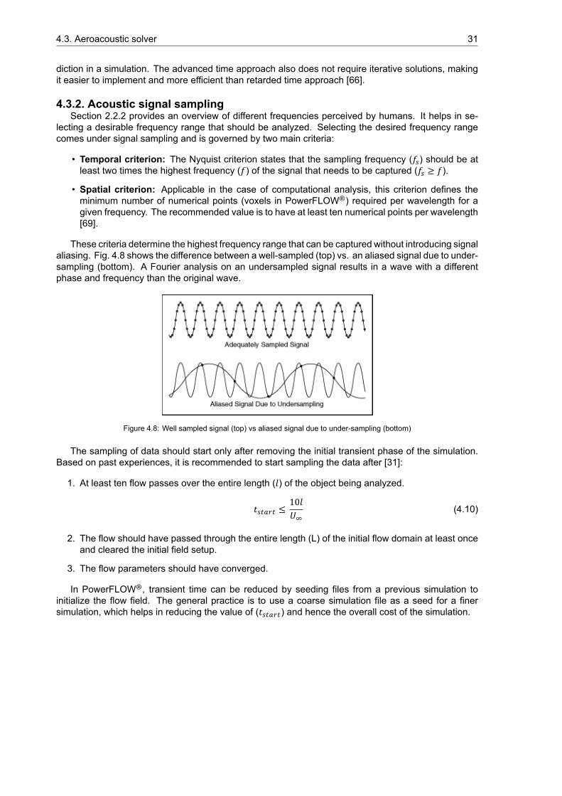
4.3. Aeroacoustic solver 31
diction in a simulation. The advanced time approach also does not require iterative solutions, makingit easier to implement and more efficient than retarded time approach [66].
4.3.2. Acoustic signal samplingSection 2.2.2 provides an overview of different frequencies perceived by humans. It helps in se-
lecting a desirable frequency range that should be analyzed. Selecting the desired frequency rangecomes under signal sampling and is governed by two main criteria:
• Temporal criterion: The Nyquist criterion states that the sampling frequency (𝑓 ) should be atleast two times the highest frequency (𝑓) of the signal that needs to be captured (𝑓 ≥ 𝑓).
• Spatial criterion: Applicable in the case of computational analysis, this criterion defines theminimum number of numerical points (voxels in PowerFLOW®) required per wavelength for agiven frequency. The recommended value is to have at least ten numerical points per wavelength[69].
These criteria determine the highest frequency range that can be captured without introducing signalaliasing. Fig. 4.8 shows the difference between a well-sampled (top) vs. an aliased signal due to under-sampling (bottom). A Fourier analysis on an undersampled signal results in a wave with a differentphase and frequency than the original wave.
Figure 4.8: Well sampled signal (top) vs aliased signal due to under-sampling (bottom)
The sampling of data should start only after removing the initial transient phase of the simulation.Based on past experiences, it is recommended to start sampling the data after [31]:
1. At least ten flow passes over the entire length (𝑙) of the object being analyzed.
𝑡 ≤ 10𝑙𝑈 (4.10)
2. The flow should have passed through the entire length (L) of the initial flow domain at least onceand cleared the initial field setup.
3. The flow parameters should have converged.
In PowerFLOW®, transient time can be reduced by seeding files from a previous simulation toinitialize the flow field. The general practice is to use a coarse simulation file as a seed for a finersimulation, which helps in reducing the value of (𝑡 ) and hence the overall cost of the simulation.

5Setup
This chapter explains the computational setup designed for the study. Section 5.1 reports the geom-etry used and the coordinate system of the setup. It is followed by a discussion on the mesh resolutionand rationale behind its selection in Section 5.2. Sections 5.3 and 5.4 introduces the reader to theboundary conditions, flow parameters, and flow measurements being saved. In Section 5.5 the exper-imental setup is presented, and parallels are drawn to the computational setup.
5.1. GeometryThe propeller chosen for this study is designed and manufactured at TU Delft. It is a twin-blade
propeller with a radius of 15 𝑐𝑚 and utilizes a NACA-4412 airfoil for its blade section. The distributionof blade angle (twist) and chord length of the propeller to the blade span is given in Fig. 5.1.
Figure 5.1: Propeller chord length and blade angle vs blade span (r/R)
The blade geometry is imported as a single-faced STL file into 𝑂𝑝𝑡𝑦𝜕𝑏®. The tool, developed by Dr.D.Casalino, segments the blade into multiple faces, referred to as Face IDs, and can add a user-definedzig-zag trip on the blade surface, see Fig. 5.2. Dividing the blade into multiple faces enables the user toset different mesh resolutions for different faces, while the trip induces flow transition. The significanceof the trip for the setup has been discussed in Section 5.1.2. Table 5.1 describes the colored sections(Face IDs) on the blade surface. The computational setup is based on an experimental study beingperformed at TU Delft. To accurately replicate the experimental setup it is decided to add a nacelle inthe computational domain instead of analyzing a stand-alone propeller, as shown in Fig. 5.3.
32

5.1. Geometry 33
Figure 5.2: Propeller blade before (top) and after (bottom) being processed by ®
Face ID Tip Root Leading Edge Trailing Edge. Laminar Section Turbulent Section
Color Purple Green Red Yellow Blue Grey
Location 2.5 % of R 20 % of R 10 % of C 5 % of C 15 % of C 70 % of C
Table 5.1: Description and location of Face IDs on the rotor blade; R = blade radius, C = local chord length
Figure 5.3: Complete geometry of the propeller setup
5.1.1. Coordinate SystemCoordinate systems are used to define the geometry and physical properties of the flow in a compu-
tation setup. This simulation utilizes three Cartesian coordinate systems to define the propeller position,simulate an AoA, and rotation of the propeller blades. The coordinate systems that have been usedare defines as follows:
• Default/Aircraft coordinate system: The default/aircraft coordinate system is the global coordi-nate system for the setup. It is the base coordinate system of the setup upon which all the othercoordinate systems are defined. In this coordinate system The z-axis is defined along the axis ofrotation and the positive y-axis and x-axis points towards Ψ = 180 and Ψ = 270 respectively,see Fig. 5.4a.
• freestream coordinate system: The setup changes the inflow angle instead of moving the pro-peller geometry to simulate an AoA. This method of defining the AoA ensures that the propellerposition stays fixed despite the change in AoA. It eliminates the need to correct the acoustic datafor distance with a change in AoA. The freestream coordinate system takes the default/aircraft co-ordinate system as its reference frame. On specifying an AoA, the freestream coordinate systemadapts its position to the default coordinate system. It modifies the inflow angle of the freestreamhence simulating an AoA. Fig. 5.4b shows the change in inflow angle relative to the propeller

34 5. Setup
geometry.
• Local Rotating reference frame (LRF): The LRF is a non-inertial rotating reference frame of thesetup. It defines the speed and direction of rotation for the propeller. For the present simulation,the RPM is 6, 000, and the propeller rotates in an anti-clockwise direction (forward-looking aft). Avolume of revolution is defined to create the LRF, such that it contains all the parts of the geometrythat will rotate relative to the inertial reference frame. Fig. 5.4c shows the direction of rotation ofthe propellers to the default coordinate system.
In this thesis, all the measurements and results discussed are relative to the default/aircraft coordi-nate system.
(a) Default/Aircraft coordinate system (b) Freestream inflow at an AoA of
(c) LRF coordinate system
Figure 5.4: Coordinate system with respect to the propeller geometry
5.1.2. Blade trippingThe nature of the flow (laminar or turbulent) over an airfoil directly impacts its aerodynamic and
aeroacoustic properties. Inherently a complex phenomenon, flow transition depends on several param-eters such as inflow condition, surface roughness, etc. [70]. LES can directly capture flow transition[71]. However, the ability comes with its own set of challenges as errors in defining the conditions oftransition in LES can give rise to artificial laminar regimes in the flow. It could induce fictitious sepa-ration of the boundary layer, severely impacting the validity of the results [72]. Forcing transition at auser-defined location helps avoid this pitfall, and study the flow characteristics with confidence.
Flow transition, in this study, is induced by placing zig-zag trips on the suction side of the propellerblades. The choice is motivated by the fact that the pressure side experiences a lower flow velocitycompared to the suction side. Hence, flow separation would be less likely. Experiments by Leslie [32]have shown that tripping the suction side of a propeller blade leads to a reduction in the high frequency(> 2, 000 𝐻𝑧) noise produced by the laminar separation bubble. 𝑂𝑝𝑡𝑦𝜕𝑏® is used to generate theseuser-defined trips. The trip properties relative to the propeller blade are shown in Fig. 5.5a.
The trip thickness of 17.41 ∗ 10 𝑚𝑚 was chosen, which has a resolution (trip thickness/ smallestvoxel size) of at least 2 voxels for coarse resolution and 4 for the highest resolution. The choice of tripthickness is driven by the belief that a minimum of 2 to 3 voxels are required to accurately resolve thetrip in the simulation [73]. The trip is placed at a relative distance of 25% of the chord length. It spansfrom 20 to 97.5% of the blade span more details about the trip have been provided in Table 5.2.
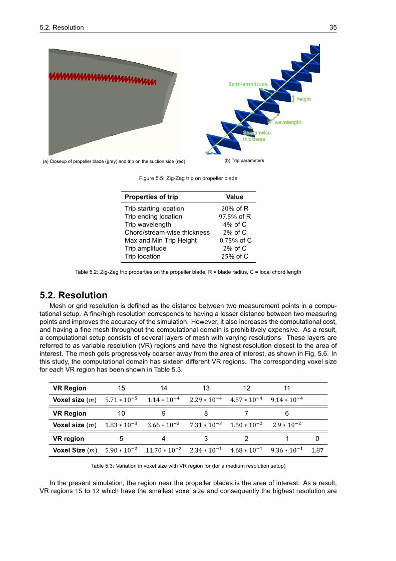
5.2. Resolution 35
(a) Closeup of propeller blade (grey) and trip on the suction side (red) (b) Trip parameters
Figure 5.5: Zig-Zag trip on propeller blade
Properties of trip ValueTrip starting location 20% of RTrip ending location 97.5% of RTrip wavelength 4% of CChord/stream-wise thickness 2% of CMax and Min Trip Height 0.75% of CTrip amplitude 2% of CTrip location 25% of C
Table 5.2: Zig-Zag trip properties on the propeller blade; R = blade radius, C = local chord length
5.2. ResolutionMesh or grid resolution is defined as the distance between two measurement points in a compu-
tational setup. A fine/high resolution corresponds to having a lesser distance between two measuringpoints and improves the accuracy of the simulation. However, it also increases the computational cost,and having a fine mesh throughout the computational domain is prohibitively expensive. As a result,a computational setup consists of several layers of mesh with varying resolutions. These layers arereferred to as variable resolution (VR) regions and have the highest resolution closest to the area ofinterest. The mesh gets progressively coarser away from the area of interest, as shown in Fig. 5.6. Inthis study, the computational domain has sixteen different VR regions. The corresponding voxel sizefor each VR region has been shown in Table 5.3.
VR Region 15 14 13 12 11
Voxel size (𝑚) 5.71 ∗ 10 1.14 ∗ 10 2.29 ∗ 10 4.57 ∗ 10 9.14 ∗ 10
VR Region 10 9 8 7 6
Voxel size (𝑚) 1.83 ∗ 10 3.66 ∗ 10 7.31 ∗ 10 1.50 ∗ 10 2.9 ∗ 10
VR region 5 4 3 2 1 0
Voxel Size (𝑚) 5.90 ∗ 10 11.70 ∗ 10 2.34 ∗ 10 4.68 ∗ 10 9.36 ∗ 10 1.87
Table 5.3: Variation in voxel size with VR region for (for a medium resolution setup)
In the present simulation, the region near the propeller blades is the area of interest. As a result,VR regions 15 to 12 which have the smallest voxel size and consequently the highest resolution are

36 5. Setup
Figure 5.6: Change in grid size with VR region; VR region in close proximity of propeller setup (left) and VR region closer to thepropeller blade (right)
placed closest to the propeller blade surface. It enables the simulation to resolve the flow field close tothe propeller blade surface and get accurate force measurements while keeping the computational costin check. To capture the tip vortices being shed by the propeller, a frustum is created in the propellerwake region. The frustum has a relatively high resolution than its surrounding (VR 11) and can be seenas the darker region on the left of Fig. 5.6. The frustum is chosen over a cylinder, as the cylinder cannot accurately capture the deflection in the propeller wake due to the change in AoA. The location andshape of the VR regions have been discussed further in Section 5.2.1.
Resolution Simulation domain size Smallest voxel Largest voxel Fine equivalent voxels(𝑚) (10 𝑚) (𝑚) (10 )
Coarse 338 ∗ 338 ∗ 338 8.1 2.6 9.8Medium 239 ∗ 239 ∗ 239 5.7 1.7 18.6Fine 168 ∗ 168 ∗ 168 4.0 1.3 36.4
Table 5.4: Variation in simulation domain and voxel size with resolution
Conducting a grid convergence/resolution study is a way of verifying the computational results. Thestudy helps find if the simulation results produced are due to the inflow and boundary conditions setby the user or a consequence of mesh resolution. If the results are invariant to the mesh density thenthe simulation is said to be grid-independent. Chapter 6 discusses the results of the resolution studyconducted on this simulation. For this study, three mesh densities were chosen (coarse, medium, andfine). The size of the voxels across the VR region changed with the mesh resolution. The size of thesimulation volume depends on the voxel size, consequently, it also varies with the mesh resolution, asshown in Table 5.4. Increasing the mesh density increases the computational cost and is computedbase on the number of fine equivalent voxels in a particular setup. The number of fine equivalent voxelsis calculated using:
Fine equivalent voxels = 𝑁( finest scale ) + 𝑁(2 finest scale )/2+𝑁(3 finest scale )/4 + 𝑁(4 finest scale)/8 + …+𝑁( coarsest )/ (2( grid levels- 1))
(5.1)
where 𝑁 corresponds to the total number of voxels in a VR region. Reduction in voxel size also impactsthe Courant–Friedrichs–Lewy (CFL) condition of the setup, resulting in an increased number of timesteps. Depending upon the hardware, an estimate of the computational time required per time step isprovided by the solver and can be seen in Table 5.5.
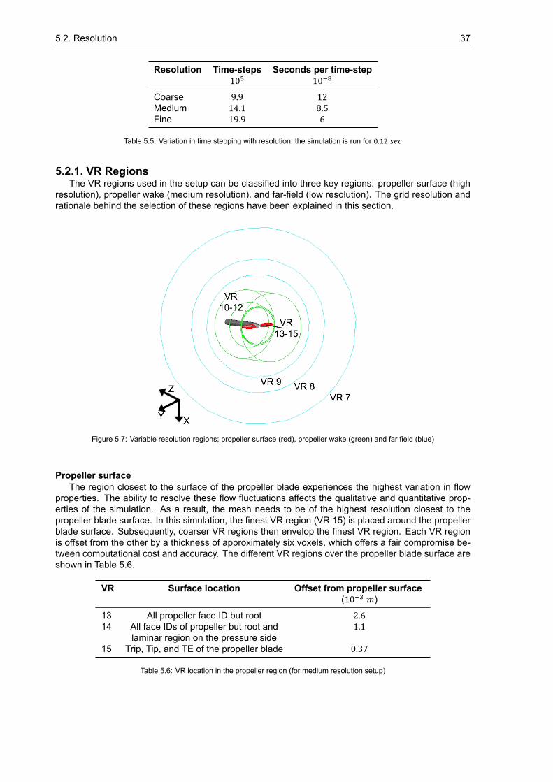
5.2. Resolution 37
Resolution Time-steps Seconds per time-step10 10
Coarse 9.9 12Medium 14.1 8.5Fine 19.9 6
Table 5.5: Variation in time stepping with resolution; the simulation is run for .
5.2.1. VR RegionsThe VR regions used in the setup can be classified into three key regions: propeller surface (high
resolution), propeller wake (medium resolution), and far-field (low resolution). The grid resolution andrationale behind the selection of these regions have been explained in this section.
Figure 5.7: Variable resolution regions; propeller surface (red), propeller wake (green) and far field (blue)
Propeller surfaceThe region closest to the surface of the propeller blade experiences the highest variation in flow
properties. The ability to resolve these flow fluctuations affects the qualitative and quantitative prop-erties of the simulation. As a result, the mesh needs to be of the highest resolution closest to thepropeller blade surface. In this simulation, the finest VR region (VR 15) is placed around the propellerblade surface. Subsequently, coarser VR regions then envelop the finest VR region. Each VR regionis offset from the other by a thickness of approximately six voxels, which offers a fair compromise be-tween computational cost and accuracy. The different VR regions over the propeller blade surface areshown in Table 5.6.
VR Surface location Offset from propeller surface(10 𝑚)
13 All propeller face ID but root 2.614 All face IDs of propeller but root and 1.1
laminar region on the pressure side15 Trip, Tip, and TE of the propeller blade 0.37
Table 5.6: VR location in the propeller region (for medium resolution setup)

38 5. Setup
Propeller wakeThe propeller wake is the region around the propeller in which the flow gets altered due to the
propeller. The relative change in flow properties in this region is lower than close to the propeller bladesurface. As a result, a relatively coarser mesh resolution can be used in this region. The region includesthe frustum to capture the tip vortices and the permeable FWH surface for the acoustic measurements.It consists of three VR regions 10, 11, and 12, as shown in green in Fig. 5.8.
Figure 5.8: Variable resolution regions; VR 12 (yellow) VR 11 (Pink)
• VR 12: it consists of all the propeller blade surfaces (including the hub) and the inner LRF of thepropeller. The VR region surrounding the propeller blade and the LRF have a thickness of 13voxels. For the medium resolution set up, they are offset by 8.5 𝑚𝑚 from the propeller surface.As the LRF is in the same VR region as the propeller blade, it does not cross two VR regions inone rotation and avoids the limitations imposed in Section 4.2.4.
• VR 11: it consists of the frustum (as described in Section 5.2) and the outer LRF of the propeller.The frustum is 1.13 times the blade radius at 𝑧/𝑅 = 0, and increases to 1.4 times the propellerradius at a distance of 𝑧/𝑅 = 1 downstream of the propeller, making an angle 15 with thepropeller axis, giving it the ability to capture the wake being deflected due to the simulated AoA.The outer LRF has a thickness of 13 voxels and an offset of 20.42 𝑚𝑚 from the propeller bladesurface for the medium resolution setup.
• VR 10: consists of a cylinder (see Fig. 5.8) that encapsulates the FWH permeable surface alongwith the transient fluid measurement region. It is 2.2 times the propeller radius and and a lengthof 0.53 𝑚, stretching from 𝑧/𝑅 = −1.8 (upstream) to 1.8 (downstream) of the propeller.
Far fieldThe far-field region starts at VR 9 and expands radially outward till VR 0. The regions from VR 9 to
VR 1 are spherical and are offset by 26 voxels from each other, whereas VR 0 is a cube. As the sizeof the domain is dependent upon the size of the voxels there is a variation in simulation domain sizeas observed in Table 5.4.
5.3. Acoustic measurementA far-field analysis of the propeller noise is carried out to understand the acoustic characteristics of
the propeller. The acoustic pressure fluctuations are sampled on a solid and permeable FWH surface,as discussed in Section 4.3.1. Acoustic measurements from the two formulations have been comparedand discussed in Section 6.2.1.
Drawing from the recommendations made in Section 4.3.2, this study uses ten numerical points(voxels) per wavelength and an aliasing safety factor of four to calculate the highest sampling frequency.The permeable surfaces are placed inside VR region 10, see Fig. 5.9, with the innermost permeable

5.4. Simulation settings 39
Figure 5.9: Acoustic setup of the simulation; 3 FWH permeable surface (red), VR 10 (green)
surface, having a radius of 0.26 𝑚. The subsequent permeable surfaces grow outwards and are offsetfrom each other by 13 voxels. The reason behind creating three permeable surfaces instead of oneis to average out the hydrodynamic noise that might be present in the sound field [74]. The pressurefluctuations in a sound field are of the order �̄�𝑐𝑈 , where �̄� is the mean pressure, 𝑐 is the speed ofsound, and 𝑈 is the local velocity fluctuation. The hydrodynamic pressure fluctuation (pseudo-noisefield) is of the order �̄�𝑈 . As the hydrodynamic noise essentially travels at fluid velocity, averaging thevalue of pressure fluctuation from the three surfaces helps remove this pseudo-noise field.
The permeable surfaces are located in VR region 10, the size of a voxel (for medium resolution) inthis region is 1.83∗10 𝑚, and the flow values in this region are sampled at 3.67∗10 𝐻𝑧. The highestsampling frequency was calculated using an aliasing safety factor of 4 and comes up to be 91, 000𝐻𝑧. However, given the location of the permeable surface, the spatial criterion determines the cutofffrequency. Table 5.7 shows the cutoff frequency as determined by the spatial criterion for different gridresolutions.
The noise radiation pattern of the propeller is captured around the propeller plane and in the axialdirection. It is done by placing two circular microphone arrays, about the XY and XZ plane, with a polarresolution of 10 and a radius of 1 𝑚 from the center of the propeller axis, see Fig. 5.9.
Resolution Spatial cutoff frequency(𝐻𝑧)
Coarse 13, 282Medium 18, 773Fine 26, 564
Table 5.7: Highest frequency set by spatial criterion at 10 voxels per wavelength
5.4. Simulation settingsThis section reports the global parameters and the boundary conditions being used for the simulation
in Sections 5.4.1 and 5.4.2. Section 5.4.3, checks for the time convergence of the simulation beforediscussing the measurements being saved in Section 5.4.4.
5.4.1. Global parametersThe values defined as the global parameters control the overall behavior of the simulation case.
These values are the characteristic physical parameters that establish reference values used to non-dimensionalize the results. For this simulation, the default turbulence intensity is set at 0.1% of the

40 5. Setup
Characteristic parameters ValuePressure 99, 000 𝑃𝑎Temperature 293 KDensity 1.18 𝐾𝑔/𝑚Kinematic viscosity 1.54 ∗ 10 𝑚 /𝑠𝑒𝑐
Table 5.8: Global characteristic parameters for the simulation
local velocity, and the turbulence length scale is set at 1 𝑚𝑚. These parameters define the turbulencecharacteristics for the fluid’s initial condition. At 0.1% of the mean velocity, the turbulence intensityreplicates a uniform inflow condition with very low freestream turbulence. The characteristic velocity iscalculated by adding the rotor tip speed, at 6, 000 RPM, to the freestream velocity. The mean chordlength of the propeller blade, at 22.85 𝑚𝑚, is set as the characteristic length (𝑙). The characteristicReynolds number is calculated to be 1.6 ∗ 10 .
5.4.2. Boundary Conditions
Characteristic parameters ValueVelocity 12 𝑚/𝑠𝑒𝑐Turbulence intensity 0.1%Turbulence length scale 1 𝑚𝑚
Table 5.9: Characteristic parameters at pressure velocity inlet
PowerCASE creates a boundary condition for each face of every solid defined in the simulation.The boundary conditions can be edited to meet the requirements of the simulation, for the presentsimulation two types of boundary conditions are used and are defined as follows:
• Standard wall: The standard adiabatic (no-slip) wall simulates a passive wall and has been usedto define the propeller geometry in the simulation.
• Pressure and velocity inlet: A solid box enclosing the entire simulation domain is created atVR region 0. The box acts as a pressure and velocity inlet for the simulation with a user-definedflow direction. It enables the face upstream of the propeller to function as an inlet and the onedownstream to act as an outlet. Table 5.9 defines the parameters used to initialize the domain;the pressure and temperature are the same as in Table 5.8.
5.4.3. Time convergenceSection 4.3.2 lists the criteria for selecting the transient time for the simulation. The mean chord
length (𝑙) of the propeller was chosen as the reference length of the object being analyzed, and at afree stream velocity of 𝑈 = 12 𝑚/𝑠𝑒𝑐, the transient time was calculated to be 2∗10 seconds. Basedon the requirements stated in point 2, for an initial flow domain of length (L) = 0.3 𝑚 the transient timewas calculated to be 2.5 ∗ 10 seconds.
The 𝐶 value for 0 and 15 AoA have been analyzed to check for time convergence of the simula-tion, see Fig. 5.10. The figure shows the values have converged well before the allotted 0.02 seconds.The fluctuation in the 𝐶 values, with respect to the mean 𝐶 , for 0 and 15 AoA case is calculated tobe 0.7% and 1.3% respectively. Based on the above values, 0.02 seconds or two propeller rotationswas chosen as the transient time of the simulation.
5.4.4. MeasurementsCFD simulations can sample multiple parameters over the entire flow domain, producing several
hundred gigabytes of data. Hence, a crucial aspect is to define the sampling domain, duration, andparameters of the simulation. It requires a trade-off between the available computational resources

5.4. Simulation settings 41
Figure 5.10: Time convergence of value at medium resolution at AoA
Measurement type Measurement duration Sampling frequency(Seconds) (𝐻𝑧)
Transient flow 0.05 7, 200FWH solid surface 0.1 3.6 ∗ 10FWH permeable surface 0.1 9.1 ∗ 10Forces 0.12 1.8 ∗ 10
Table 5.10: Measurement type for the simulation domain; Sampling frequency for the medium resolution setup
and the measurements required to understand the flow characteristics. The measurements saved forall simulations during this study are shown in Table 5.10.
Transient Flow: The transient flow measurement records the fluid and surface variable within avolume enclosed by it. Fig. 5.11 shows the part (in pink) used to define the transient measurementvolume. The cylinder has a volume of 5.9 ∗ 10 𝑚 , and extends from 𝑧/𝑅 = −3.3 in front of thepropeller plane to 𝑧/𝑅 = 2 aft of it. It samples and saves parameters such as density, velocity, vorticity,forces (only for surface), and pressure. The sampling frequency of 7, 200 𝐻𝑧 gives it a polar resolutionof 5 .
Figure 5.11: Fluid measurement setup; transient measurement volume (pink), VR 10 (green)
FWH solid surface: The FWH solid surface samples the pressure.FWH permeable surface: It samples the pressure, density, and velocity over its surface without

42 5. Setup
influencing the flow.Forces: The forces measurement type samples the forces and moments experienced by the pro-
peller blade surface.
5.5. Experimental setupThe experimental setup designed by Edoardo Grande of the TU Delft aeroacoustics group is used
for validating the computational results. This section provides an overview of the experimental setupthat has been used for the purpose. The setup consists of a twin-bladed propeller, as reported inSection 5.1, supported by a strut enclosed in a nacelle placed at the TU Delft anechoic wind tunnel.The main difference between the experimental and the computational propellers is the absence of azig-zag trip on the experimental setup. The zig-zag trips could be a potential source of variation in theaerodynamic and acoustic result and shall be discussed further in Chapter 6.
For the acoustic measurements, two microphone arrays are placed in the wind tunnel to performbeam-forming (Array 1) and find the directivity of the noise (Array 2). In the computational study, acous-tic data is compared by replicating Array 2 from the experimental setup. Mic 5 on Array 2 is located ata distance of 1.5 𝑚 from the propeller axis (at 0 AoA). The array has a radius of 3.5 times the propellerdiameter, measured at a distance of 45 𝑐𝑚 from the center of the propeller axis. Tables A.1 and A.2provides the exact locations of the microphones used in Array 2 in the default/aircraft coordinate systemused in this thesis.
Figure 5.12: Experimental Setup
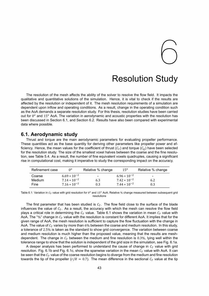
6Resolution Study
The resolution of the mesh affects the ability of the solver to resolve the flow field. It impacts thequalitative and quantitative solutions of the simulation. Hence, it is vital to check if the results areaffected by the resolution or independent of it. The mesh resolution requirements of a simulation aredependent upon inflow and operating conditions. As a result, change in the operating condition suchas the AoA demands a separate resolution study. For this thesis, resolution studies have been carriedout for 0 and 15 AoA. The variation in aerodynamic and acoustic properties with the resolution hasbeen discussed in Section 6.1, and Section 6.2. Results have also been compared with experimentaldata where possible.
6.1. Aerodynamic studyThrust and torque are the main aerodynamic parameters for evaluating propeller performance.
These quantities act as the base quantity for deriving other parameters like propeller power and ef-ficiency. Hence, the mean values for the coefficient of thrust (𝐶 ) and torque (𝐶 ) have been selectedfor the resolution study. The size of the smallest voxel halves between the coarse and the fine resolu-tion, see Table 5.4. As a result, the number of fine equivalent voxels quadruples, causing a significantrise in computational cost, making it imperative to study the corresponding impact on the accuracy.
Refinement case 0 Relative % change 15 Relative % change
Coarse 6.69 ∗ 10 - 6.96 ∗ 10 -Medium 7.14 ∗ 10 6.3 7.42 ∗ 10 6.2Fine 7.16 ∗ 10 0.3 7.44 ∗ 10 0.3
Table 6.1: Variation in value with grid resolution for and AoA; Relative% change measured between subsequent gridresolutions
The first parameter that has been studied is 𝐶 . The flow field close to the surface of the bladeinfluences the value of 𝐶 . As a result, the accuracy with which the mesh can resolve the flow fieldplays a critical role in determining the 𝐶 value. Table 6.1 shows the variation in mean 𝐶 value withAoA. The ”%” change in 𝐶 value with the resolution is constant for different AoA. It implies that for thegiven range of AoA, the mesh resolution is sufficient to capture the flow fluctuation with the change inAoA. The value of 𝐶 varies by more than 6% between the coarse and medium resolution. In this study,a tolerance of 2.5% is taken as the standard to show grid convergence. The variation between coarseand medium resolution is much higher than the proposed value, meaning that the results are mesh-dependent. The change in 𝐶 between the medium and fine resolution is 0.3%, lying well within thetolerance range to show that the solution is independent of the grid size in the simulation, see Fig. 6.1a.
A deeper analysis has been performed to understand the cause of change in 𝐶 value with gridresolution. Fig. 6.1b and Fig. 6.1c, show the spanwise variation in the mean 𝐶 value with AoA. It canbe seen that the 𝐶 value of the coarse resolution begins to diverge from the medium and fine resolutiontowards the tip of the propeller (𝑟/𝑅 = 0.7). The mean difference in the sectional 𝐶 value at the tip
43

44 6. Resolution Study
region (𝑟/𝑅 = 0.8 to 1) is around 16% between the coarse and the medium resolution setup for the twoAoAs. The propeller blade experiences the highest velocity due to the rotation of the propeller at thetip region. It results in significantly higher variation in the flow field compared to the root and mid-spansection of the propeller blade. The coarse mesh is unable to resolve these variations in the flow field,which results in the underprediction of the velocity magnitude around the propeller blade causing areduction in the calculated 𝐶 value. The phenomenon can be visualized using the Lambda-2 vortexcriterion (Λ ), which uses a three-dimensional velocity field to identify vortices using a vortex core linedetection algorithm. Fig. 6.2, visualizes the vortices close to the propeller blade surface at Λ = −1∗101/𝑠𝑒𝑐 . It can be seen through the figure that the vortices detected by the Λ criterion are significantlylarger than the medium and fine resolution setup. The large size is a result of the higher jump in velocityexperienced while calculating the velocity field due to the larger grid size. Signifying the inability of thegrid resolve the small-scale fluctuation in the flow field.
(a) Variation of overall with grid resolution
(b) Variation of across blade span with grid resolution at AoA (c) Variation of across blade span with grid resolution at AoA
Figure 6.1: Variation of value with grid resolution
Figure 6.2: Vortex visualization for different resolution at = ∗ /sec for ; Suction side of propeller blade.
The next parameter that has been studied is 𝐶 . It is a measure of the resistance to rotation expe-rienced by a propeller and determines the power required to drive it. The value of 𝐶 varies by around

6.2. Aeroacoustic study 45
4% between coarse and medium resolution at 0 AoA and 5% at 15 AoA. The change in 𝐶 valueis limited to about 2% between the medium and fine resolution setup for both AoAs, see Fig. 6.3a.Analyzing the span-wise distribution of 𝐶 shows that the coarse resolution slightly over predicts thetorque value in the propeller mid-span (𝑟/𝑅 = 0.4 − 0.7), and the value is under-predicted in the tipregion, as shown in Figs. 6.3b and 6.3c. The observed variation can be explained using the samehypothesis proposed for the observed variation in 𝐶 . The value of aerodynamic forces shows a goodconvergence for the medium resolution setup based on a computational cost vs. accuracy tradeoffof the medium resolution setup is a viable choice for aerodynamic analysis. After verifying that theaerodynamic results are independent of the grid size, they are validated against experimental data.
(a) Variation of overall with grid resolution
(b) Variation of across blade span with grid resolution at AoA (c) Variation of across blade span with grid resolution at AoA
Figure 6.3: Variation of value with grid resolution
Table 6.2 presents the comparison between experimental and computational force coefficients. The𝐶 value has been over-predicted in the simulation by 9−10%, whereas the 𝐶 value is underpredictedby 8.5%. The difference in 𝐶 value can be associated with the different boundary-layer conditions overthe experimental and computational propellers. In the computational setup, the boundary layer is forcedto transition using a zig-zag strip, whereas the flow is allowed to transition naturally in the experiment. Itcould potentially mean that the flow remains laminar in the experimental case for a significantly higherpercentage of the chord length than in the simulation. Turbulent BL exerts higher shear stress on thepropeller surface and produces a higher skin friction drag than laminar BL. Therefore, justifying thevariation in 𝐶 value between the experimental and computational results. The 𝐶 value is dependentprimarily upon the lift produced by the propeller blade section, which in turn depends upon the pressuredistribution over the blade surface. The presence of a trip acts as an obstruction to the flow over thepropeller blade surface resulting in a jump in the 𝐶 value on the suction side. This in turn could impactthe overall pressure distribution over the propeller blade surface.
6.2. Aeroacoustic studyUnderstanding the acoustic characteristics of the propeller is a critical part of this study. Hence, it is
vital to study the impact of FWH integration surface and grid resolution on the acoustic results. A powerspectrum (PS) analysis is performed on the noise signal to examine its tonal and broadband content. It

46 6. Resolution Study
0 15Experimental Computational Variation Experimental Computational (%)
𝐶 7.8 ∗ 10 7.1 ∗ 10 −8.5% 8.1 ∗ 10 7.4 ∗ 10 −8.4𝐶 7.7 ∗ 10 8.5 ∗ 10 9.3% 7.7 ∗ 10 8.6 ∗ 10 10.6
Table 6.2: Force comparison between experimental and computational result; Variations measured wrt. experimental andsimulation values
calculates the energy within the specified frequency bandwidth (Δ𝑓) to generate a spectrum plot of thesignal. As opposed to power spectral density (PSD) which calculates the energy of the signal per unitfrequency. The advantage PS offers is that changing the frequency bandwidth (Δ𝑓) of the analysis doesnot affect the tonal noise levels in a PS analysis, while in PSD the tonal noise levels change with Δ𝑓.As tonal noise tends to dominate the OASPL in propeller noise, using PS makes it easier to comparenoise levels. In this thesis, the PS analysis has a frequency bandwidth (Δ𝑓) of 20 𝐻𝑧 and a range of40 − 10, 000 𝐻𝑧.
This section is divided into two sub-parts Section 6.2.1 analyses the acoustic results from solid(FWH SLD) and permeable(FWH PRM) surfaces and decides upon the FWH formulation that shall beused throughout this thesis. Section 6.2.2 studies the impact of grid resolution on the acoustic resultsand decides upon the grid resolution that shall be used for further analysis.
6.2.1. FWH surface selectionSection 4.3.1 discussed how the FWH analogy is implemented in PowerFLOW® through the for-
mulation of solid and permeable integration surfaces. In this section, the far-field noise captured bythe integration surfaces is calculated using two circular microphone arrays described in Section 5.3. Acomparison between their OASPL is performed, followed by a power spectrum analysis to understandthe observed variations.
(a) Difference around propeller plane (b) Difference along axial direction
Figure 6.4: Difference in OASPL between solid and permeable FWH integration surface
The OASPL is a measure of the total energy contained in the spectrum. To compare the noisesignal captured by the two integrating surfaces, the OASPL for a frequency range of 40 - 10, 000 𝐻𝑧 iscalculated using the circular microphone arrays. It is observed that the OASPL of the solid integrationsurface is higher than that captured by the permeable surface. Fig. 6.4, plots the difference in OASPL(FWH SLD - FWH PRM) in the propeller plane and along the axial direction. In the propeller plane,at 0 AoA, the difference between FWH SLD and FWH PRM surface is around 1.4 𝑑𝐵, showing littleto no variation with azimuthal angle (Ψ). However, at an AoA of 15 , the difference in OASPL variesby over 2 𝑑𝐵 with a change in azimuthal angle. It fluctuates between 0.85 𝑑𝐵 at Ψ = 120 to 2.96 𝑑𝐵at Ψ = 280 , as shown in Fig. 6.4a. In the axial plane, along the free stream direction, the differencein FWH SLD and FWH PRM OASPL acquires a lobular structure. In the top half of the axial plane

6.2. Aeroacoustic study 47
(𝜃 = 0 → 90 → 180 ), the lobes show a maximum difference of 4.4 𝑑𝐵 (𝛼 = 0 ) and 3.1 𝑑𝐵 (𝛼 = 15 )at 𝜃 = 140 . The difference increases to 7 𝑑𝐵 for 𝛼 = 15 at 𝜃 = 250 , while it remains the same for0 AoA, 4.4 𝑑𝐵 at 𝜃 = 240 , in the lower half of the axial plane (𝜃 = 180 → 270 → 0 ). A commonobservation from Fig. 6.4a and Fig. 6.4b is that the difference in OASPL increases in the direction ofthe wake, i.e. the permeable surface underpredicts the OASPL values in the downstream direction.
(a) Power spectrum around propeller plane; at AoA (b) Power spectrum along axial plane; at AoA
Figure 6.5: Power spectrum of solid and permeable FWH integration surface; =
To better understand the cause of this difference in OASPL, a power spectrum analysis is performedon the noise signal. The power spectrum analysis is performed for a frequency range of 40 − 10, 000𝐻𝑧 using a Hanning window with 50% overlap and a frequency bandwidth Δ𝑓 of 20 𝐻𝑧, as shown inFig. 6.5. The power spectrum curves are in good agreement with each other in the high-frequencyregion. It is because the quadrupole source terms scale to the eighth power of Mach number. Giventhe low Mach number (< 0.3) of the present simulation, it is not a surprise that the quadrupole sourcesdo not play a dominant role in determining the high-frequency range of the power spectrum. As a result,the inability of FWH-SLD to capture the quadrupole source terms has no impact on broadband noiseor the OASPL of the signal. The difference in power spectrum level is primarily observed in the low-frequency region. At Ψ = 280 (𝛼 = 15 ) the difference in SPL at 1 BPF is 3 𝑑𝐵, which is the sameas the total difference in OASPL between FWH SLD and FWH PRM surfaces, as shown in Fig. 6.5a.A similar observation is made along the axial direction as well. Fig. 6.5b show the power spectrum atΘ = 260 (for 𝛼 = 15 ), the difference in SPL at 1 and 2 BPF is about 5 𝑑𝐵, whereas the broadbandpart of the signal are in good agreement.
The computational results clearly show the difference in OASPL measurements of the solid andpermeable FWH integration surface. However, these results can not justify the choice of one integrationsurface over another. Hence, the computational results of both integration surfaces are comparedagainst experimental data obtained by Edoardo Grande. Fig. 6.6 shows the comparison between thenoise signals captured by the two FWH integration surfaces and experimental measurements. In thedownstream location (Mic number 1), the solid surface is in excellent agreement with the experimentalresults, whereas the permeable surface under-predicts the OASPL (𝑓 = 40 − 1, 000 𝐻𝑧) by 10 𝑑𝐵.The results show similar trends observed in the computational results, where the permeable surfaceunderpredicted the tonal component of the propeller noise. Moving in the upstream direction (Mic 1 →Mic 8), the OASPL values of the solid surface begin to diverge from the experimental results and is inbetter agreement with the permeable surface. A power spectrum analysis is performed on the noisesignal to understand its cause and analyze the energy content in different frequencies.
In the upstream direction at Mic 1 the FWH SDL shows good agreement with the experimentalresult at 1 and 2 BPF, the agreement however deteriorates towards higher harmonics. The higherharmonic tones observed in the experimental data could be attributed to factors such as; i) Proximityof the propeller blades to the wind tunnel shear layer at 15 AoA; ii) Vibrations in the experimentalsetup resulting in unsteady loading on the propeller blades; causing higher harmonic noise. Thesefactors are not present in the computational simulation and can justify the observed variation in SPL atharmonics of BPF. Moving downstream, towards Mic 8, the difference in SPL between the experimentaland solid surface increases to 7 𝑑𝐵 at 2 BPF, rising to over 20 𝑑𝐵 for subsequent harmonics. It

48 6. Resolution Study
(a) OASPL measurements for ,
(b) Power spectrum level at microphone number ; (c) Power spectrum level at microphone number ;
Figure 6.6: Comparison between solid (SLD), permeable (PRM), and experimental (EXP) noise data at AoA
results in the difference in the OASPL values observed in Fig. 6.6a. The FWH PRM surface constantlyunderpredicts the tones at 1 and 2 BPF in the downstream direction, and the OASPL value at Mic1 is 11 𝑑𝐵 less than the experimental value. The permeable surface data seems to be corrupted by thepropeller wake. Individual analysis of the acoustic data obtained by the three integration surfaces, seeFig. A.4, showed a similar trend of under-predicting tonal noise in the direction of the propeller wake.Consequently, averaging the values from the three FWH PRM surface does little to correct the data.
Through the power spectrum analysis, it is clear that the solid integration surface has the bestagreement with the experimental result.It captures the 1 BPF tone to within 1 𝑑𝐵 of the experimentalmeasurements at 15 AoA and has a similar directivity to the experimental values. Hence, the acousticdata captured by the FWH solid surface is used for studying the noise generated by the propeller inthis thesis.
6.2.2. Grid selectionThe present section analyses the effect of grid resolution on acoustic results. Based on conclusions
of Section 6.2.1, the FWH SLD integration surface has been used to analyze the results in this section.The resolution study is carried out for coarse, medium, and fine resolution for microphones placed at𝜃 = 90 and 110 . Fig. 6.7a, shows the variation in OASPL (40 − 10, 000 𝐻𝑧) and SPL at 1 BPF forboth the microphones. The OASPL and SPL at 1 BPF vary by less than 0.5 𝑑𝐵 between the coarse,medium, and fine resolution setup. At higher frequency, the agreement of SPL deteriorates significantlywith the resolution, see Fig. 6.7b. At a frequency range of 1, 500 − 2, 500 𝐻𝑧, the SPL varies by 6 𝑑𝐵between the coarse and the medium resolution. The variation reduces to 3 𝑑𝐵 between medium andfine resolution.
The solid FWH integration surface, due to its proximity to the propeller blade, lies in VR region12. It ensures that the cutoff frequency for all the resolutions in the setup is above 10, 000 𝐻𝑧, hencethe variation in sampling frequency can not justify the difference in broadband noise levels with gridresolution. A power spectrum analysis is performed on the pressure values obtained from the propellerblade surface to understand the cause of variation in SPL with grid resolution. A frequency bandwidth(Δ𝑓) of 1, 000 𝐻𝑧, is used for analysing a frequency range of 1, 000 − 10, 000 𝐻𝑧. Fig. 6.8a shows the

6.2. Aeroacoustic study 49
(a) Variation in OASPL and BPF with grid resolution; Solid linesrepresent & dotted line represent AoA;
(b) Variation in spectrum level with resolution ( , AoA = ,)
(c) Variation in broadband noise ( , , ) with grid resolution.
Figure 6.7: Variation in acoustic result with grid resolution at
surface pressure distribution (in 𝑑𝐵), obtained for a frequency range of 1, 500 − 2, 500 𝐻𝑧 for coarse,medium, and fine resolution setup. It is observed that the blade surface pressure at the trailing edge forhigher frequencies (1, 000 − 10, 000 𝐻𝑧) increases with decreasing resolution. The surface pressurefluctuation at the trailing edge of a propeller is a significant source of broadband noise [9]. Thesefluctuations are produced due to the downstream convection and formation of a turbulent boundarylayer over the blade surface. A plausible explanation for the variation in broadband noise with theresolution is that the coarse resolution setup is unable to resolve the small-scale turbulence presentin the turbulent boundary layer. The larger turbulent structures result in higher pressure fluctuationsas they convent downstream from the propeller blade trailing edge into the wake, resulting in higherbroadband noise. Fig. 6.8b attempts to picture this phenomenon by overlaying vortices visualized byΛ vortex criterion. It can be observed that at Λ = −4 ∗ 10 1/𝑠𝑒𝑐 the coarse resolution is unable toresolve the smaller flow structures like the medium and the fine resolution setup. The same analogycan be applied to the flow structures present in the turbulent boundary layer as well. Another reasonfor it could be the low trip resolution for the coarse mesh. With only two voxels to cover the trip, the tripstep might not be completely resolved in the simulation affecting the flow transition and consequentlythe turbulent BL.
From the OASPL values, it can be stated that the coarse resolution is sufficient for capturing theacoustic data. However, since the aerodynamic data converges at medium resolution and the changein broadband noise is also significantly lower at this resolution, the medium resolution setup is used foranalyzing the acoustic results in the present study.

50 6. Resolution Study
(a) Surface pressure fluctuation (dB) on the suction side of the propeller blade.
(b) Surface pressure fluctuation ( ) map with vortex visualisation at ∗ /sec
Figure 6.8: Surface pressure fluctuation ( ) at AoA for a frequency range of , , ; contour range 60 dB,suction side of the propeller blade.

7Results
This chapter discusses the aerodynamic and acoustic results obtained from simulations. It is dividedinto three sections, Sections 7.1 and 7.2 discusses the aerodynamic results in terms of the forcesexperienced by the propeller blade and flow field analysis, and Section 7.3 discusses the aeroacousticresults.
7.1. Propeller forceThe forces experienced by a propeller depend upon its RPM and inflow conditions. When the
propeller operates at a non-zero AoA, relative to the freestream, the freestream velocity consists ofcomponents that act parallel and perpendicular to the propeller disc. These components change theeffective blade AoA of the propeller, causing a variation in blade loading around the azimuthal (Ψ) plane.Operating at 6, 000 RPM at a freestream velocity of 12 𝑚/𝑠𝑒𝑐, changing the AoA from 0 to 15 resultsin an increase in mean thrust by 3.87%, while the torque required increases by 1.16%. It shows that thetorque values are less sensitive to the changes in AoA when compared to thrust values. As a result,the propeller experiences a net increase in its propulsive efficiency with a change in AoA. Table 7.1,shows the mean thrust, torque, and efficiency values obtained for the two AoAs.
15 0 DifferenceAoA AoA (%)
𝐶 7.4 ∗ 10 7.1 ∗ 10 3.87Thrust (𝑁) 7.11 6.84𝐶 8.6 ∗ 10 8.5 ∗ 10 1.16Torque (𝑁𝑚) 0.25 0.24𝜂 (%) 54.88 53.66 1.22
Table 7.1: Mean thrust, torque and propeller efficiency value for propeller; % difference calculated between and AoA
Operating at an AoA, the propeller plane can be classified into two main parts, the advancing bladeside, and the retreating blade side. The classification is based upon the variation in resultant velocityand AoA experienced by the propeller blades due to the change in freestream velocity componentsaround its azimuthal position. On the advancing side, the propeller experiences an increase in itsresultant velocity and AoA over the blade section, resulting in higher thrust. The conditions reverse onthe retreating side. Appendix A, explains the concept of advancing and retreating side in detail throughvelocity triangles. The simplistic calculation based on the propellers velocity triangles identified thatthe propeller blade operating at Ψ = 270 → 0 → 90 (advancing side) will experience higher bladeloading than propeller operating at Ψ = 90 → 180 → 270 (retreating side).
Fig. 7.1, quantifies the change in sectional 𝐶 and 𝐶 values as the propeller blade rotates aroundthe propeller plane. As the sectional variation of 𝐶 around the propeller plane remains constant at 0AoA, the value at Ψ = 0 is chosen as the reference value. For 15 AoA, Ψ = 0 , 90 , 180 , and 270are chosen to study the variation in sectional thrust and torque values with AoA. The propeller blade is
51

52 7. Results
divided into three sections, root (𝑟/𝑅 = 0− 0.4), mid-span (𝑟/𝑅 = 0.4 − 0.8), and tip (𝑟/𝑅 = 0.8 − 1), toget better insight into how the aerodynamic forces vary across the blade. At Ψ = 0 for 15 AoA, thepropeller blade experiences significantly higher thrust and torque relative to 0 AoA. The thrust valuesat the root vary by 45% it gradually reduces to 22% at the mid-span and 16% at the tip. A similarobservation is made at Ψ = 180 . The thrust values are lower by 32% at the root, 13.8% at mid-span,and 9.3% at the tip relative to 0 AoA. Though the sectional variation in thrust values is expected avariation of over 30% at the root section deserves further examination.
(a) value across blade span at different for and (b) value across blade span at different for and
Figure 7.1: Variation in sectional and with azimuthal angle ( ) for and
The thrust produced is directly dependent upon the lift (𝐶 ) and drag (𝐶 ) force experienced bythe propeller blade section. The sectional 𝐶 and 𝐶 value is a function of the resultant velocity overthe propeller blade section. It is determined by the components of the freestream velocity and localrotational speed of the propeller and influences the AoA and Reynolds number of the blade section. Atthe tip region, the rotational speed dominates over the freestream velocity component. Consequently,the effect of change in propeller AoA is reduced on the sectional blade AoA towards the tip region, seeFig. A.5. At the root section, the velocity induced by the propeller rotation is the smallest. It resultsin the root section experiencing the highest variation in resultant velocity due to AoA. The change inresultant velocity also influences the Reynolds number. Studies into the aerodynamic characteristic oflow Reynolds number airfoil show an exponential rise in 𝐶 /𝐶 value in the Reynolds number range of5 ∗ 10 to 10 [44]. In this case, the average Reynolds number in the root region at Ψ = 0 is 8.5 ∗ 10at 0 it increases to 9.7 ∗ 10 for 15 . Fig. 3.9b shows that this region experiences one of the highestincreases in 𝐶 /𝐶 value with Reynolds number. Hence the variation of thrust value by over 30% atthe root section can be justified by the combined influence of the Reynolds number effect and highervariation in the region.
The above paragraph explained the variation of aerodynamic forces along the blade span. However,it does not quantify the net effect of these forces on the propeller plane. Fig. 7.2a shows the total thrustforce produced by a propeller blade as it rotates around the propeller plane. At 0 AoA the bladeproduces a steady thrust of 3.4 newtons, at 15 AoA the thrust force varies between 2.8 newtons atΨ = 198 (minimum) to 4.3 newtons atΨ = 17 (maximum). Showing a 35% change in loading aroundthe azimuthal position. The maximum and minimum loads experienced by the propeller blade lead tocyclic loading of the propeller, as seen in Fig. 7.2b. However, upon analyzing Fig. 7.2b it is observedthat the net fluctuation in thrust force for the propeller around the azimuth is less than 1% for 15 AoA.It is because the point of minimum and maximum loading have an azimuthal distance of 180 . As aresult, for a twin-bladed propeller, the net force balances out between these locations.
7.2. Flow field analysisThe propeller flow field is analyzed by visualizing the velocity field and vortices produced by the
propeller. The velocity field is obtained by averaging the flow field values for a period of five propellerrotations. To visualize, the vortex field a phase-locked analysis is performed on the transient flow

7.2. Flow field analysis 53
(a) Net thrust force produced by a single propeller blade with changingazimuthal angle ( ) (b) Propeller per rotation
Figure 7.2: Change in thrust values with azimuthal angle ( )
field. The vortices are then detected using the Lambda-2 vortex criterion. The analysis is performed inthe axial direction and along the propeller plane of symmetry. Section 7.2.1 discusses the changes invelocity, and Section 7.2.2 discusses the changes in vortices produced by the propeller. In Section 7.2.3the effects of the change in AoA on the surface pressure fluctuations of the blade surface are analyzed.
7.2.1. Velocity fieldThe flow velocity in the propeller slipstream is an important parameter to describe the flow field in
that region. It captures the variations caused due to the addition of momentum into the flow field by thepropellers. In this section, the averaged velocity field behind the propeller is analyzed to quantify andunderstand the effect of AoA on the flow field. The transient flow measurement has been averaged outfor five propeller rotations to obtain the mean flow presented in this section. The velocity contours soobtained are captured along the propeller plane of symmetry as well as the axial direction and analyzed.
Figure 7.3: Axial velocity profile for and AoA
Fig. 7.3 captures the velocity profile along the propeller plane of symmetry. At 0 AoA, the propellerwake is symmetric about the 𝑋𝑍 and 𝑌𝑍 planes. Hence, a single plane is sufficient to visualize thevelocity field. Operating at 15 AoA, varying blade loads about Ψ leads to a non-symmetric velocityfield. Hence, both 𝑋𝑍 and 𝑌𝑍 planes are used for analyzing the velocity field for 15 AoA. The velocityfield has been non-dimensionalized using the free stream velocity (𝑈 = 12 𝑚/𝑠𝑒𝑐 along the 𝑧 axis).Operating at 6, 000 RPM, at 0 AoA, the propeller accelerates the flow to 1.4 times the freestreamvelocity at 𝑧/𝑅 = 0.2, where 𝑧 is the distance along the positive 𝑍-axis, and 𝑅 is the radius of the

54 7. Results
propeller. As the wake travels downstream, the trailing edge vortices present in the flow start to breakdown and transfers energy into the flow field, which is partially responsible for the increase in theslipstream velocity to 1.6 time the freestream velocity at 𝑧/𝑅 > 1. At 15 AoA, the non-axial freestream velocity causes the propeller blade to experience varying loads around the propeller plane anddeflects the wake produced. To capture these phenomena the propeller velocity profile is capturedalong the 𝑌𝑍 as well as the 𝑋𝑍 plane Fig. 7.3 a) and b) respectively. The results in Section 7.1 showedthat the propeller experiences higher loading at Ψ = 0 (advancing side) than at Ψ = 180 (retreatingside). The asymmetry in loading around the propeller plane results in an asymmetric velocity fieldabout the propeller axis, as seen in Fig. 7.3 a). The velocity magnitude is up to 6% higher at 𝑧/𝑅 = 0.3in the advancing side compared to the retreating side. As the wake travels downstream, the velocitymagnitude close to the nacelle on the retreating side shows a significant rise (around two times thefreestream velocity) compared to the advancing side. It is because of the energy transferred into theflow by the root vortex interacting with the nacelle. This interaction is caused by the deflection ofpropeller wake by the oncoming freestream at 15 AoA, as seen in Fig. 7.3 b).
Themean velocity field is captured at different locations along the axial direction to develop a deeperunderstanding of how the flow develops along the axial direction. Fig. 7.4 shows the evolution of thevelocity field at 𝑧/𝑅 = 0.2, 0.6 and 1 for 0 and 15 AoA. The velocity magnitude is visualized for arange of 12− 20 𝑚/𝑠𝑒𝑐, as it highlights the variations in the mean velocity field. The white spots in thevelocity plots are regions where the mean velocity is less than the freestream velocity.
(a) AoA
(b) AoA
Figure 7.4: Velocity magnitude at different radial position along the propeller axis
Fig. 7.4a captures the mean velocity field at 0 AoA for the above-mentioned axial locations. At𝑧/𝑅 = 0.2, the mean velocity is 1.3 times the freestream velocity in the wake of the propeller. It leadsto a 9% contraction in the propeller stream tube compared to the propeller diameter. As the wakemoves downstream, the trailing edge vortices produced by the propeller blades dissipate and transferenergy into the wake. At 0 AoA, the root and tip vortices produced by the propeller remain coherentin the entire measurement region. It prevents the flow in the freestream from mixing with the propeller

7.2. Flow field analysis 55
wake. Which results in the formation of two distinct velocity bands in the propeller was at 𝑟/𝑅 < 0.2and 𝑟/𝑅 > 0.8, as seen in Fig. 7.4a.
Fig. 7.4b shows the velocity field in the wake of the propeller at 15 AoA. A distinguishing featureof the flow field at 15 is the asymmetric nature of the velocity field. At 𝑧/𝑅 = 0.2 the velocity fieldstarts to show a higher mean velocity close to the root region (𝑟/𝑅 = 0.2 − 0.4) on the advancing sideof the propeller plane (Ψ = 270 → 0 → 90 ). As the wake moves downstream the asymmetricin the velocity field becomes more evident. Examination of Figs. 7.2a and 7.4b establishes a clearcorrelation between the influence of blade loading on the downstream velocity profile. As the bladeloading reduces between Ψ = 180 to 240 so does the mean velocity magnitude. The inflow angle ofthe freestream velocity deflects the propeller wake, which results in the break down of the root vortexaround Ψ = 0 → 90 → 180 . It causes the observed rise in mean velocity close to the nacelle. Thenature of the vortices shed by the propeller, and the impact of AoA shall be discussed in more detail inSection 7.2.2.
7.2.2. Vortex fieldIn the present section snapshots of the instantaneous flow field are captured to analyze the vor-
tices being shed by the propeller. The analysis is carried along the propeller axis on the 𝑋𝑍 plane ofsymmetry. A phase-locked analysis is carried out on the transient flow field for a period of five pro-peller rotations to isolate the periodic fluctuations in the flow field. A measuring window spanning from𝑧/𝑅 = −0.1 (ahead of the propeller) to 𝑧/𝑅 = 1.7 (behind the propeller) is used to capture the vor-tices. The vortices being produced by the propellers are visualized using the Lambda-2 (Λ ) vortexvisualization technique.
Fig. 7.5 captures the evolution of the vortices produced by the propeller along the freestream. Thevorticity magnitude (𝜔) is non-dimensionalized using a reference value of 500, which is obtained bydividing the freestream velocity of the simulation by the characteristic length. At 15 , due to the changein inflow angle, the propeller wake is pushed towards the positive 𝑋-axis. The root vortex and nacelleinteraction result in the root vortex breaking down into smaller vortical structures. The inflow angle alsoresults in the formation of stronger vortices at the propeller hub. The two phenomena create a region ofhigh vorticity at 𝑧/𝑅 = 0.4 to 0.8. Despite the high vorticity, it has minimal contribution to the broadbandnoise due to the low flow velocity. The breaking up of the root vortex and downward deflection of thetip vortices can be visualized by Fig. 7.6.
Figure 7.5: Vorticity magnitude along the propeller axis
Using the Λ vortex criterion the vortices in the fluid domain are identified using the three-dimensionalvelocity field. In Fig. 7.6 the Λ value is set at −1∗10 1/𝑠𝑒𝑐 , the color contour represents the velocitymagnitude of the shed vortex. The tip vortex exhibits a similar structure and velocity profile at 0 and15 AoA. The only difference is the downward deflection of the vortices and the breaking up of the root

56 7. Results
vortices, which have been discussed in the previous sections. To understand the nature of the trailingedge vortices a closer look is taken at the propeller blade section for 15 and 0 AoA at Ψ = 0 . Thetrailing edge vortices at the tip region (𝑟/𝑅 > 0.8) of the propeller convect at three times the freestreamvelocity and exhibit the same characteristics for 0 and 15 AoA. At the root section (0.0 > 𝑟/𝑅 > 0.4),there are visible differences in the vortices being shed. At 15 the trailing edge vortices are convectedat approximately 2.5 times the freestream velocity, whereas it is less than two times the freestreamvelocity at 0 . The vortex structure and shape at the trailing edge also differ for 0 and 15 AoA. Thevortices produced at the leading edge of the propeller blade experiences higher convective velocity at15 AoA than at 0 . It could lead to variation in surface pressure fluctuation over the blade surface,which in turn can affect the noise produced by the propeller blade. The following section discusses thevariation in blade surface pressure fluctuation for 0 and 15 AoA.
Figure 7.6: Vortex visualization for and AoA at ∗ / and
7.2.3. Surface pressure fluctuationThe force fluctuations over a propeller blade surface due to fluctuating surface pressure is a dom-
inant acoustic source. In this section, the variation in blade surface pressure fluctuation is analyzedfor 0 and 15 AoA across the blade span to understand how the AoA impacts the surface pressurefluctuation at different frequencies. The blade surface pressure values are obtained for 0.1 seconds (10rotations) at a sampling frequency of 3.6 ∗ 10 𝐻𝑧. The pressure fluctuations captured are reported inthe 𝑑𝐵 scale set against a reference value of 2∗10 𝑃𝑎, and the contour plot over the blade surface hasa range of 60 𝑑𝐵. A power spectrum analysis is performed on the surface pressure values that convertthe pressure signal from the time domain to the frequency domain and helps analyze the energy contentof selected frequency bands. The analysis is performed for a high-frequency band (1, 500−7, 500 𝐻𝑧),with a frequency bandwidth (Δ𝑓) of 1, 000 𝐻𝑧, and a low frequency band (100−700 𝐻𝑧) with Δ𝑓 = 200𝐻𝑧. The segregation of the analysis into high and low-frequency helps in understanding the chord andspanwise distribution of the surface pressure fluctuation for different frequency bands and the impactof AoA on it.
For 𝑓 = 100−300 𝐻𝑧 pressure fluctuations at the leading edge dominate the blade surface pressurefluctuation at 15 AoA, see Fig. 7.7. It remains a significant source till 𝑓 = 500 − 700 𝐻𝑧 at which thelow-pressure fluctuation is almost uniformly distributed over the blade surface. At 0 the contributionof the propeller leading edge to the low-pressure fluctuation is significantly reduced, and the blade

7.3. Acoustics 57
(a) Surface pressure fluctuation ( ) on the suction side of the propeller blade at AoA
(b) Surface pressure fluctuation ( ) on the suction side of the propeller blade at AoA
Figure 7.7: Surface pressure fluctuation ( ) at , and BPF; contour range 60
section aft of the trip becomes a more dominant contributor. A plausible explanation of this behavioris the change in AoA experienced by the propeller blade around the azimuthal plane while operatingat 15 AoA. The change in AoA results in a periodically varying pressure field over the propeller blade.The leading edge of the propeller experiences the maximum variation in pressure with change in AoA.Justifying the dominating contribution of the leading edge to low-pressure fluctuation. Since a propellerblade operating at 0 AoA does not experience any such variation about its azimuthal position, there isno significant pressure fluctuation at the blade’s leading edge. The root section of the propeller bladeis also a region of particular interest. Section 7.1 discusses the significant variation in 𝐶 value at theroot section of the propeller blade, Section 7.2.2 also pointed out the difference in vortex structures inthe same region. Figs. 7.7a and 7.7b shows the discrepancy in the surface pressure fluctuation for thetwo AoA at the root region. At 0 AoA, the root section experiences significantly lower surface pressurefluctuation than 15 AoA. The difference could be a potential source of noise, which shall be discussedin Section 7.3.
Fig. 7.8 captures the surface pressure fluctuation over the propeller blade surface at 𝑓 > 1, 000𝐻𝑧 contributing to the broadband noise spectrum. For 0 AoA, the pressure fluctuation over the pro-peller blade surface does not change significantly with frequency. The pressure fluctuation is at itsminimum close to the blade root and increases towards the tip region. The trailing edge of the propellerblade at the tip region experiences maximum pressure fluctuation. Hence, contributing the most to thetrailing edge broadband noise produced by the propeller. At 15 AoA, the pressure fluctuation showsconsiderable variation, between 1, 500 − 4, 500 𝐻𝑧. The change is minimal at the higher frequencyrange, 4, 500 − 7, 500 𝐻𝑧, and starts to resemble the pressure fluctuation distribution at 0 AoA. Forthe frequency range between 1, 500 − 4, 500 𝐻𝑧, the propeller blade at 15 AoA experiences a higherpressure fluctuation at the root section than 0 AoA. The magnitude of the pressure fluctuation reduceswith an increase in frequency. However, at 15 AoA, the trailing edge region towards the propeller tipexperiences the highest pressure fluctuation. It is similar in magnitude to that of the propeller bladeat 0 AoA. As this section contributes the most to the broadband part of the acoustic spectrum, it isa possibility that the propeller blades exhibit similar broadband characteristics despite the change inAoA.
7.3. AcousticsThis section analyzes and quantifies the changes that occur in the acoustic characteristic of the
propellers with AoA. Section 7.3.1 discusses and quantifies the difference in the noise produced by thepropeller across its blade span. Sections 7.3.2 and 7.3.3 analyzes the variation in the directivity of thenoise generated by the propeller along its axial and radial plane.

58 7. Results
(a) Surface pressure fluctuation ( ) on the suction side of the propeller blade at AoA
(b) Surface pressure fluctuation ( ) on the suction side of the propeller blade at AoA
Figure 7.8: Surface pressure fluctuation ( ) between , , at , interval; contour range .
7.3.1. Source noiseSections 7.1 and 7.2 discussed how the forces and flow parameters varied across the propeller
blade with a change in AoA. The present section quantifies those variations in terms of the sound powerlevel (PWL) across the propeller blade span. Measured against a reference value of 10 watts, thePWL is measured using the 𝑑𝐵 scale. The difference between PWL and SPL is their dependenciesupon distance. SPL measures the pressure fluctuation produced by a sound wave when it reachesa receiver, it depends upon the distance between the source and the receiver. PWL measures theamount of energy produced by a source of the sound and is independent of the distance between thesource and observer. PWL is hence preferred to measure the variation in the source strength (propellerblade) with a change in AoA.
(a) Sectional sound power level (b) Integrated sound power level over the blade span
Figure 7.9: Sound power level across a the propeller blade
Fig. 7.9 presents the sectional (Fig. 7.9a) and integrated (Fig. 7.9b) PWL across the propeller bladespan for 0 and 15 AoA. The PWL is calculated by segmenting the propeller blade across its span using

7.3. Acoustics 59
the structured mesh generated by the 𝑂𝑝𝑡𝑦𝜕𝑏® package and then calculating the pressure fluctuationover the individual sections. The structured mesh at the root (𝑟/𝑅 = 0 − 0.2) and tip (𝑟/𝑅 = 0.975 − 1)section of the propeller blade are not segmented like the rest of the blade span. It results in the regionhaving a relatively larger area than the rest of the segmented blade section, causing the peak in the PWLvalues at the root and tip section, as observed in Fig. 7.9a. Analysis of the sectional PWL reveals thatsignificantly higher noise is generated at the root region. For 𝑟/𝑅 = 0− 0.4 the average PWL between0 to 15 varies by 7 𝑑𝐵, with the difference rising close to 13 𝑑𝐵 near the root and reducing to 3 𝑑𝐵closer to 𝑟/𝑅 = 0.4. The increase in surface pressure fluctuation at 15 observed in Section 7.2.3 canbe a plausible explanation for the higher PWL level in the same region. Moving towards the tip, thedifference in sectional PWL collapses to less than 2 𝑑𝐵, which again follows a similar trend observedby the surface pressure fluctuations. The net noise produced by the propeller blade at 15 AoA is 83𝑑𝐵, which is 1.5 𝑑𝐵 higher than the noise produced by it at 0 AoA. It implies that the variation in PWLat the root region has a marginal impact on the overall PWL of the propeller blade. The effect changein AoA has on the directivity of noise shall be explored in the following sections.
7.3.2. Radial directivityThe present section analyses the variation in the OASPL with AoA around the radial plane. It is
measured for a frequency range of 40 − 10, 000 𝐻𝑧 using a circular microphone array of 1 𝑚 radius.In the present simulation, the AoA is changed by varying the inflow angle instead of changing thepropeller position. As a result, the distance of the microphones wrt. the propellers remain constant.It eliminates a source of uncertainty caused in the measurements due to the relative shift in propellerlocation. The directivity analysis is divided into a low-frequency (40 − 1, 000 𝐻𝑧) and high-frequency(1, 000 − 10, 000 𝐻𝑧) plot. It is done to analyze the influence of frequency on directivity and find thedominating component of the OASPL.
Figure 7.10: Radial directivity of OASPL; frequency range a) , b) , , c) , ;measured at from the propeller axis of rotation;
Fig. 7.10a shows the radial directivity of the noise produced by the first five BPF (40 − 1, 000𝐻𝑧)of the propeller. Fig. 7.10b shows the directivity of the high-frequency noise produced by the propeller(1, 000 − 10, 000 𝐻𝑧). The OASPL for 40 − 10, 000 𝐻𝑧 is present in Fig. 7.10c. A comparison of thedirectivity plots reveals that the low-frequency noise dominates the OASPL in the radial direction. Thebroadband noise shows no variation in directivity with a change in AoA. At 0 AoA, the propeller exhibitsa symmetric directivity pattern about the plane of rotation. However, at 15 , the directivity patternbecomes non-axisymmetric about Ψ = 0−180 axis. The OASPL in the propeller plane lying betweenΨ = 0 − 90 − 180 is relatively higher at 15 than 0 AoA. The OASPL value reaches its highestvalue at Ψ = 90 , where the OASPL is 3 𝑑𝐵 higher for 15 AoA. The point of maximum variation is thesame as predicted by [9] and no phase lead/lag is observed in the simulated as seen by [10, 11]. It isbecause of the difference in the measurement conditions and the type of propeller blades. Experimentsby Woodward [10] and Mani [11] were conducted for large turboprops with multiple propeller bladesand a significantly higher inflow and tip Mach number. A large number of blades operating at high tip

60 7. Results
Mach numbers result in the propeller blades interacting with the wake produced by the other blades. Itleads to the propeller blade experiencing unsteady loading, causing noise in higher harmonics of BPF.The unsteady noise also leads to the phase lead/lag effect observed by [10]. The present simulationuses a twin-blade propeller with a maximum tip Mach number of 0.3 and a freestream velocity of 12𝑚/𝑠𝑒𝑐. Visualizing the vortex field produced by the propeller in Section 7.2.2 made it apparent thatthe freestream velocity leads to the downstream convection of the vortices before they interact with thepropeller blade. It reduces the impulsive change in propeller blade loading due to wake interaction,hence removing a source of unsteady noise that would cause tonal peaks at higher harmonics.
Fig. 7.11 presents the power spectrum analysis of the noise signal at three different azimuthal po-sitions. The spectrum analysis is performed at a frequency bandwidth of Δ𝑓 = 20 𝐻𝑧. It reveals theenergy content of each frequency band and helps understand their variation across the azimuthal po-sition. Based on the directivity plot in Fig. 7.10, power spectrum analysis of microphones placed atΨ = 90 , 180 and 270 has been performed. The analysis reveals that the change in SPL level withthe azimuthal position is restricted to mainly the 1 and 2 BPF. At Ψ = 90 the tonal peak, at 1BPF, of the propeller is higher by 3 𝑑𝐵 for 15 AoA and is reduced by an equal magnitude at Ψ = 270 .The power spectrum plot for both 15 and 0 AoA, show three distinct tonal peaks at multiples of BPFwith minimal difference in the spectrum at a higher frequency. It is in line with the observation madein Section 7.2.3 that the propeller blades would exhibit similar broadband characteristics despite thechange in operational AoA.
Figure 7.11: Variation in spectrum level around the propeller plane
7.3.3. Axial directivityIn the present section, the directivity of the OASPL is analyzed along the propeller axis in the 𝑋𝑍
plane. The analysis is performed using a circular array of 36 microphones, using the same methodol-ogy described in Section 7.3.2. In a CAA simulation, microphones do not disturb the flow. As a result,it is feasible to place microphones upstream of the propeller plane. The ability enables a 360 analy-sis of the OASPL along the propeller axis, which is extremely difficult, if not impossible to achieve inexperiments.
Fig. 7.12a, b, & c represents the variation of the OASPL for 0 and 15 around the 𝑋𝑍 plane for afrequency range of 40−1, 000 𝐻𝑧,1, 000−10, 000 𝐻𝑧, and 40−10, 000 𝐻𝑧 respectively. The directivityplot for the low and high-frequency range in Fig. 7.12a & b exhibit a dipolar noise radiation patternassociated with steady loading and broadband noise, respectively. In the low frequency region thevariation in the tonal noise is similar to that observed around the propeller plane, with 𝜃 = 0 → 90 →180 experiencing higher noise than 𝜃 = 180 → 270 → 0 . As the propeller location remains thesame wrt. the microphone, the change in directivity can be attributed to the relative change in pressureamplitude produced by the propeller blade due to the changes in propeller tip Mach number and bladeAoA. Another interesting observation is the dominance of broadband noise in the axial directivity ofnoise in the forward and aft direction. For 𝜃 = 330 → 0 → 30 and 𝜃 = 150 → 180 → 210the broadband noise is significantly higher than the tonal component. It is due to the dipolar nature ofthe two acoustic sources and the 90 phase difference due to the difference in their noise generationmechanism, as discussed in Section 3.1.2.
Fig. 7.13 presents the noise spectra for the signal at 𝜃 = 90 , 0 and 270 . For 𝜃 = 0 it canbe observed that there is a lack of tonal peak in the power spectrum plot. It is due to the destructiveinterference of the pressure wave-forms produced by the propeller blades which are equal in magnitude

7.3. Acoustics 61
Figure 7.12: Axial directivity of OASPL; frequency range a) , b) , , c) , ;measured at from the propeller axis of rotation;
Figure 7.13: Variation in noise spectra along the axial direction
but opposite in phase. However, at 15 AoA, there is an asymmetry in the blade loading about thepropeller plane, which results in the singular tonal peak observed for 15 AoA.

8Conclusions and Recommendations
The present chapter consists of the conclusions drawn from the result of this study and makes rec-ommendations for the extension of this work. The conclusion drawn from the study has been presentedin terms of the research questions listed out in Section 3.3. Section 8.2 discusses the scope of expan-sion of the present study and additional analysis that can be carried out to understand the aerodynamicand aeroacoustics characteristics of propeller operating at low Reynolds number.
8.1. ConclusionsThis section aims to answer the research questions set in Chapter 3 by concluding the results
discussed in Chapters 6 and 7. The research questions and their answers have been discussed below:
1. What is the computational resource required in conducting a study of the impact of AoAon aerodynamics and acoustic characteristics of a low Reynolds number propeller?
• What is the required grid resolution to accurately capture all the flow phenomena?– In this study, three different grid resolutions were analyzed to check for grid indepen-dence and validated against experimental data. The medium resolution set up with18.6 ∗ 10 fine equivalent voxels, with the smallest voxel size of 5.7 ∗ 10 𝑚 was foundsufficient in capturing all the flow phenomena.
• What is the impact on the accuracy of results with changes in grid resolution?– The value of 𝐶 was under-predicted by 6.3% in the coarse setup compared with themedium resolution setup. The difference in 𝐶 value was limited to 0.3% between themedium and fine resolution setup. At 2% the 𝐶 values showed slightly higher variationbetween the medium and fine resolution setup. However, these were within accept-able levels to prove for grid independence of the results. To check for the accuracy ofthe force coefficient were compared against experimental data. It was found that themedium resolution setup under-predicted the 𝐶 values by 8.5% and over-predicted 𝐶value by 9.3%. These values indicate a reduction in the accuracy of the simulation withreducing grid resolution.The coarse resolution setup is unable to resolve the smaller flow structures close tothe propeller blade. It results in the variation in force coefficients with grid resolutionfor the simulations. The differences in force coefficients between the experimental andsimulation results could be due to the difference in flow characteristics over the propellerblade. The difference occurs due to the forced transitioning of the flow over the propellerblade surface in the simulation.In terms of acoustic values, the low-frequency tonal noise shows a negligible variationwith grid resolution. The tonal noise dominates the noise spectrum, consequently, theOASPL (from 40 − 10, 000 𝐻𝑧) also remains steady with the change in grid resolution.The broadband OASPL is higher by 6 𝑑𝐵 (for 1, 500−2, 500 𝐻𝑧) for the coarse resolutionwrt. the medium resolution. The coarse resolution setup is unable to resolve small-scale
62

8.1. Conclusions 63
turbulence close to the propeller blade. It results in higher pressure fluctuations alongthe blade trailing edge resulting in higher broadband noise generation.
• How does the variation in AoA impact the accuracy of the results at a similar grid resolution?– The variation in AoA had a negligible impact on the accuracy of the results for similargrid resolution. It signifies that the medium resolution setup can be used for the entirerange of AoA (0 − 15 ) with similar flow conditions.
2. What is the impact on Aerodynamics characteristics of the propeller with a change in AoA
• What impact does a change in AoA have on the overall performance and efficiency of thepropeller?– The change in AoA, from 0 to 15 , increases the thrust produced by the propeller from6.84 to 7.11 𝑁. The 3.87% increase in the net 𝐶 value per rotation is accompanied byan increase in 𝐶 value by 1.16%. It results in an overall increase in propeller efficiencyfrom 53.66% to 54.88%.
• How does the thrust and torque value vary across the propeller blade with a change in AoAand azimuthal position?– The propeller blade exhibits a cyclic variation in blade loading around the propeller plane.It experiences maximum loading of 4.3 𝑁 at Ψ = 17 and 2.8 𝑁 at Ψ = 198 , which is a35% variation between the point of maximum and minimum loading. In terms of span-wise variation of thrust and torque value, the maximum % variation with AoA occursat the root region, followed by the mid-span and the propeller tip region. The coupledinfluence of the Reynolds number effect and higher variation in resultant velocity at theroot region (0 < 𝑟/𝑅 < 0.4) results in over 30% variation in the sectional thrust value atΨ = 0 for 0 and 15 AoA.
• What is the impact of the change in AoA on the flow filed?– The flow field is analyzed by visualizing the mean velocity and phase-locked vorticityin the wake of the propeller. The velocity field is axially symmetric for 0 AoA aboutthe 𝑋𝑍 and 𝑌𝑍 plane of symmetry. For 15 AoA, the average velocity field is no longeraxisymmetric about the plane of symmetry. The asymmetry in propeller blade loadingleads to a 6% higher velocity magnitude in the advancing side (Ψ = 270 → 0 → 90 )of the 𝑌𝑍 plane. Analyzing the mean velocity shows a clear correlation between bladeloading and mean velocity. The asymmetry of the downstream velocity field replicatesthe blade loading pattern about the propeller plane.The tip vortices being shed by the propeller no significant variation in strength and re-main coherent for 0 and 15 AoA. The change in AoA has a visible impact on thedownstream convection of the root vortex. The change in inflow angle, at 15 , causesthe root vortex to interact with the support structure. It results in the breakdown of thecoherent vortical structure and acceleration of the flow close to the support strut. Theinflow angle has a relatively higher influence on the resultant velocity and blade loadingin the root region (0 < 𝑟/𝑅 < 0.4) of the propeller. It results in a significant variationin the vortices produced in this region. A consequence of this is the change in surfacepressure fluctuation and hence the noise generated by the propeller blade.
3. What is the impact on the acoustic characteristics of the propeller with a change in AoA?
• How does the sound power level (PWL) produced by the propeller change with AoA? Howdoes it relate to the aerodynamic characteristics of the propeller blade?– The average PWL in the root region (0 < 𝑟/𝑅 < 0.4) of the propeller varies by 7 𝑑𝐵between 0 and 15 AoA. The sectional measurements shows that the PWL for 15AoA is 13 𝑑𝐵 higher at 𝑟/𝑅 = 0.2 as compared to 0 AoA. The difference reduces to3 𝑑𝐵 at 𝑟/𝑅 = 0.4 and is less than 1 𝑑𝐵 as it moves closer to the tip. The net PWLincreases by 1.5 𝑑𝐵 for the propeller blade at 15 AoA as compared to 0 AoA.The sound produced is directly dependent upon the amount of pressure fluctuation pro-duced by the source. Hence, the observed variation in PWL was correlated against the

64 8. Conclusions and Recommendations
surface pressure fluctuation map for different frequency ranges. The pressure fluctu-ation on the propeller blade surface showed similar trends of variation with change inAoA. The pressure fluctuations in the root region of the propeller showed significantlyhigher variation with change in AoA. It can be attributed to the relatively higher changesin resultant flow velocity and blade loading in this region.
• How does the axial and radial directivity of the noise produced change with changing AoA?– In the radial plane, the tonal component dominates the OASPL and directivity of noise.The change in AoA leads to an asymmetry in the noise radiation pattern in the radialplane. The OASPL is higher by 3 𝑑𝐵 at Ψ = 90 for 15 AoA and reduces by an equalmagnitude at Ψ = 270 . The variation is limited to the 1 and 2 BPF tones of thepropeller noise. The Broadband spectrum shows a negligible variation with change inAoA. It is expected as the surface pressure fluctuation on the propeller blade in thehigh-frequency region is almost identical at higher magnitudes closer to the tip of thepropeller.In the axial direction, a similar trend is observed for directivity as in the radial plane. Thebroadband noise dominates the OASPL directly aft and in front of the propeller blade.The tonal noise in this region is similar in magnitude but opposite in phase. It leads tothe cancellation of the tonal peaks resulting in lower tonal noise.
• What changes occur in the SPL levels of higher harmonics due to change in AoA?– The variation in higher harmonics is primarily caused due to impulsive changes in load-ing caused due to turbulent inflow conditions, Blade vortex interaction, etc. In the presentsimulation due to a relatively high freestream velocity of 12 𝑚/𝑠𝑒𝑐 and a uniform inflowcondition. The propeller blades do not experience any impulsive change in blade load-ing despite the change in AoA. As a result, there is no change in higher harmonics witha change in AoA.
8.2. RecommendationsThis section lists out the various recommendations that can help expand on the present study and
further enhance the understanding of the effect of inflow angle on low Reynolds number propeller:
• Trip placement: in the present study the trip is placed at the quarter chord length on the suctionside of the propeller blade. To analyse the effect of trip on the aerodynamics and acoustic char-acteristics, the trip position can be changed to better suite the natural transition point of the flow.Trips can also be added on the pressure side of the blades and results compared with untrippedsimulation.
• Change in AoA and RPM: due to time and resource constraint, this study only analysed twoAoAs at fixed RPM and freestream velocity. The study can be expanded further to includemultipleAoAs, advance ratio (𝐽), and hover condition. Doing so would help develop a better understandingof the impact of inflow condition on the propeller acoustics. Analysing the propeller at hovercondition for different AoAs would also help capture additional sources of noise such as bladevortex interaction, etc.
• Numerical beamforming: Numerical beamforming can be applied in the simulation to isolate thesource of noise for a specific frequency range across the propeller blade span. It would enhancethe understanding of the regions producing noise and the subsequent impact of AoA on them.
• Development of low fidelity model: high fidelity tools are resource-intensive and are not suit-able for preliminary design and getting quick estimates. The results of the present study can beused to validate low fidelity models for propellers operating in non-axial inflow conditions. Sincelow fidelity tools require significantly lesser computational resources, they can be used in con-junction with other low fidelity models to get reasonable estimates on UAV performance early onin the design phase.

AAppendix
This section aims to provide additional information to support the concepts/points discussed in thereport.
Microphone locationThe microphone locations of ARRAY-2 in the computational domain wrt. the default co-ordinate
system.
Microphone X-Axis Y-Axis Z-Axis 𝜃Number (𝑚) (𝑚) (𝑚) ( )
1 1.12 0 0.80 234.442 1.28 0 0.64 243.523 1.40 0 0.44 252.494 1.47 0 0.23 261.245 1.5 0 0 06 1.47 0 -0.23 278.767 1.40 0 -0.44 287.518 1.28 0 -0.64 296.48
Table A.1: Microphone location of ARRAY 2 in the simulation domain at
Microphone X-Axis Y-Axis Z-Axis 𝜃Number (𝑚) (𝑚) (𝑚) ( )
1 1.12 0.8 0.80 234.442 1.28 0.91 0.64 243.523 1.40 1 0.44 252.494 1.47 1.04 0.23 261.245 1.5 1.06 0 06 1.47 1.04 -0.23 278.767 1.40 1 -0.44 287.518 1.28 0.91 -0.64 296.48
Table A.2: Microphone location of ARRAY 2 in the simulation domain at
NASA SR series propellersDuring the 1980s researchers at NASA developed a series of advanced propellers that were studied
for their aerodynamic and acoustics characteristics. These propellers were known as the SR series of
65

66 A
propellers. The literature reviewed for this thesis has analyzed the SR-2 and SR-7A series of propellers.The SR-7A propeller is similar to the SR-3 propeller [10]. Figure A.1 shows the blade profile of thedifferent SR series propeller blades.
Figure A.1: NASA SR series propeller blades[8]
The SR-7A and SR-2 propeller used by Woodward [10] and Whitefield [11] had a diameter of 62.2𝑐𝑚, designed Mach number of 0.8, and a designed tip speed of 244 𝑚/𝑠𝑒𝑐.
Advancing and retreating sideIn the computational setup, the inflow AoA is changed to simulate the effect of AoA, and the propeller
blades rotate in a counter-clockwise direction, as shown in Figs. A.2a and A.2b. AoA can also besimulated by keeping the inflow angle constant and changing the propeller AoA as shown in Fig. A.2c.
(a) Schematic representation of inflow induced AoA
(b) Propeller view (forward looking aft)
(c) Schematic diagram of propeller induced AoA
Figure A.2: Simulating AoA in the computational setup
To explain the concept of advancing and retreating sides, the resultant velocity and AoA will becalculated using velocity triangles. The calculations are performed at a radial location (𝑟/𝑅) of 0.53and azimuthal position of Ψ = 0 and 180 for 0 and 15 AoA. Fig. A.3a, shows the inclination ofthe propeller shaft relative to the freestream. The airfoil marked in red moves downwards (towardsΨ = 270 ), whereas the one marked in blue moves upwards (towards Ψ = 90 ). At 𝛼 = 0 , thepropeller experiences uniform loading around the propeller plane. Fig. A.3b shows the resultant velocity(𝑉 ) for the propeller blade element at 𝑟/𝑅 = 0.53. At 𝛼 = 15 , the propeller blade experiences varying

A 67
loads around the propeller plane. The loads vary due to the change in local AoA and resultant velocityexperienced by the propeller at the different azimuthal positions. Figs. A.3c and A.3d show the variationin resultant velocity and the corresponding change in AoA between the downward moving propellerblade (at Ψ = 180 ) and upwards moving propeller blade at (Ψ = 0 ). The downward moving bladeexperiences a lower resultant velocity over the blade section as compared to the upwards moving bladeit results in a lower AoA and hence lower blade loading. The advancing side refers to the section ofthe propeller plane where the blades experience higher blade loading (Ψ = 270 → 0 → 90 ), whileΨ = 90 → 180 → 270 is defined as the retreating side.
(a) Close up view of the propeller at an AoA(b) Propeller blade at
(c) Propeller blade at moving downwards, (d) Propeller blade at moving upwards,
Figure A.3: Variation in AoA and resultant velocity for propellers with an AoA
Permeable vs solid surface acoustic dataFig. A.4, shows the difference in SPL between the solid and permeable FWH surface. The differ-
ences calculated are for each permeable integration surface instead of averaging the contribution of allthree surfaces.
Sectional blade AoAFig. A.5, shows the average variation in sectional blade AoA around the azimuthal plane (Ψ).

68 A
(a) Difference between FWH SLD and FWH PRM (b) Difference between FWH SLD and FWH PRM
(c) Difference between FWH SLD and FWH PRM
Figure A.4: Difference between FWH SLD and the the three individual FWH PRM surface
Figure A.5: Average change in AoA across blade span.
Axial velocity profileFig. A.6 shows the average velocity profile in the propeller slipstream along the axial direction. The
average has been calculated for five propeller rotations.

A 69
(a) Axial velocity profile at AoA (b) Axial velocity profile at AoA
Figure A.6: Mean axial velocity profile in the propeller slipstream

BAppendix
This section provides the formulas for the different non-dimensional parameters used throughoutthe thesis.
Non-dimensional parametersCoefficient of thrust (𝐶 )
𝐶 = 𝑇𝜌𝑛 𝐷 (B.1)
Coefficient of Torque (𝐶 )
𝐶 = 𝑄𝜌𝑛 𝐷 (B.2)
Advance ratio (𝐽)For axial inflow condition:
𝐽 = 𝑈𝑛𝐷 (B.3)
𝐽 = 𝑈 𝑐𝑜𝑠(𝛼)𝑛𝐷 (B.4)
where 𝛼 is the AoA.
Propeller efficiency (𝜂)The propeller efficiency is the ratio of the power supplied (𝑃 ) to the use-full output produced by the
propeller (𝑃 ), and is defined as:
𝜂 = 𝑃𝑃 (B.5)
it can be calculated using:
𝜂 = 12𝜋𝐶𝐶 𝐽 (B.6)
Non-dimensional velocity
Velocity [-] = 𝑈𝑈 (B.7)
𝑈 defines the velocity being measured.
70

B 71
Non-dimensional vorticity
Vorticity [-] = 𝜔𝜔∗ (B.8)
𝜔 is the compute vorticity magnitude, and 𝜔∗ is calculated as:
𝜔∗ = 𝑙𝑈 (B.9)
𝑙 is the characteristic length at 23 𝑚𝑚, and 𝑈 is the freestream velocity at 12 𝑚/𝑠𝑒𝑐.
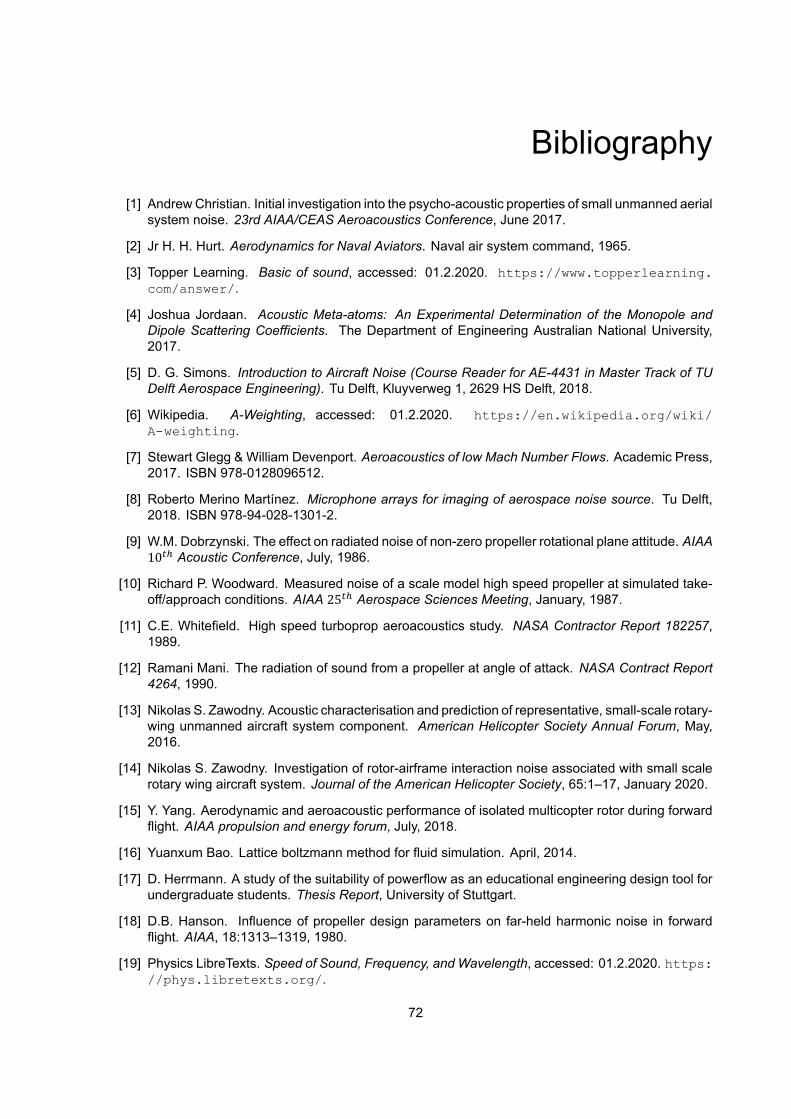
Bibliography[1] AndrewChristian. Initial investigation into the psycho-acoustic properties of small unmanned aerial
system noise. 23rd AIAA/CEAS Aeroacoustics Conference, June 2017.
[2] Jr H. H. Hurt. Aerodynamics for Naval Aviators. Naval air system command, 1965.
[3] Topper Learning. Basic of sound, accessed: 01.2.2020. https://www.topperlearning.com/answer/.
[4] Joshua Jordaan. Acoustic Meta-atoms: An Experimental Determination of the Monopole andDipole Scattering Coefficients. The Department of Engineering Australian National University,2017.
[5] D. G. Simons. Introduction to Aircraft Noise (Course Reader for AE-4431 in Master Track of TUDelft Aerospace Engineering). Tu Delft, Kluyverweg 1, 2629 HS Delft, 2018.
[6] Wikipedia. A-Weighting, accessed: 01.2.2020. https://en.wikipedia.org/wiki/A-weighting.
[7] Stewart Glegg & William Devenport. Aeroacoustics of low Mach Number Flows. Academic Press,2017. ISBN 978-0128096512.
[8] Roberto Merino Martínez. Microphone arrays for imaging of aerospace noise source. Tu Delft,2018. ISBN 978-94-028-1301-2.
[9] W.M. Dobrzynski. The effect on radiated noise of non-zero propeller rotational plane attitude. AIAA10 Acoustic Conference, July, 1986.
[10] Richard P. Woodward. Measured noise of a scale model high speed propeller at simulated take-off/approach conditions. AIAA 25 Aerospace Sciences Meeting, January, 1987.
[11] C.E. Whitefield. High speed turboprop aeroacoustics study. NASA Contractor Report 182257,1989.
[12] Ramani Mani. The radiation of sound from a propeller at angle of attack. NASA Contract Report4264, 1990.
[13] Nikolas S. Zawodny. Acoustic characterisation and prediction of representative, small-scale rotary-wing unmanned aircraft system component. American Helicopter Society Annual Forum, May,2016.
[14] Nikolas S. Zawodny. Investigation of rotor-airframe interaction noise associated with small scalerotary wing aircraft system. Journal of the American Helicopter Society, 65:1–17, January 2020.
[15] Y. Yang. Aerodynamic and aeroacoustic performance of isolated multicopter rotor during forwardflight. AIAA propulsion and energy forum, July, 2018.
[16] Yuanxum Bao. Lattice boltzmann method for fluid simulation. April, 2014.
[17] D. Herrmann. A study of the suitability of powerflow as an educational engineering design tool forundergraduate students. Thesis Report, University of Stuttgart.
[18] D.B. Hanson. Influence of propeller design parameters on far-held harmonic noise in forwardflight. AIAA, 18:1313–1319, 1980.
[19] Physics LibreTexts. Speed of Sound, Frequency, and Wavelength, accessed: 01.2.2020. https://phys.libretexts.org/.
72

Bibliography 73
[20] Commercial drone market size, share trends analysis report by application (filming photography,inspection maintenance), by product (fixed-wing, rotary blade hybrid), by end use, and segmentforecasts, 2019 - 2025. https://www.grandviewresearch.com/industry-analysis/global-commercial-drones-market, Accessed: September 2020.
[21] John F. Groeneweg. Aeroacoustics of advanced propellers. 17th Congress of the internationalCouncil of Aeronautical Sciences, 1990.
[22] D.B. Hanson. Sound from propeller at angle of attack: a new theoretical viewpoint. The RoyalSociety, pages 315–328, 1995.
[23] Eugene A. Krejsa. Prediction of the noise from a propeller at angle of attack. 13th AeroacousticsConference, 1990.
[24] Simon Marié. Comparison between lattice boltzmann method and navier–stokes high orderschemes for computational aeroacoustics. Journal of Computational Physics, 228, 2009.
[25] Flight Standards Service U.S. Dept. of Transportation, FAA. Pilot’s Handbook of AeronauticalKnowledge. FAA.
[26] Frank E. Hitchens. Propeller Aerodynamics: The history of Aerodynamics and operations of air-craft propellers. Andrews UK Limited, 2015.
[27] D. Russell. Acoustic monopoles, dipoles, and quadrupoles: An experiment revisited. AmericanJournal of Physics, 1999.
[28] Jack E. Marte & Donald W. kurtz. A Review of Aerodynamic Noise from Propellers, Rotors, andLift Fans. NASA, Jet Propulsion Laboratory, Cal. Tech, Pasadena, california, 1970.
[29] Thomas F. brooks. Airfoil self-noise and prediction. NASA Technical reports, 1989. doi:19890016302.
[30] S. Oerlemans. Location and quantification of noise sources on a wind turbine. Journal of Soundand Vibration, 299, 2007.
[31] W. C. P. van der Velden. Computational aeroacoustic approaches for wind turbine blade noiseprediction. Tu Delft, 2017. ISBN 978-94-6186-756-8.
[32] Angus Leslie. Broadband noise reduction from a mini-uav propeller through boundary layer trip-ping. Acoustics 2008, November 2008.
[33] Oleg A. Godin. An exact wave equation for sound in inhomogeneous , moving, and non-stationaryfluids. OCEANS’11 MTS/IEEE KONA, 2011.
[34] M. J. Lighthill. On sound generated aerodynamically .i general theory. The royal society mathe-matical physical & Engineering sciences, 222, 1952.
[35] M. J. Lighthill. On sound generated aerodynamically .ii turbulence as a source of sound. The royalsociety mathematical physical & Engineering sciences, 211, 1954.
[36] M.S. Howe. Theory of vortex sound. Cambridge university press, 2002. ISBN 9780521012232.
[37] A. Hirschberg & S.W. Rienstra. An introduction to aeroacoustics. Eindhoven University of Tech-nology, 2004.
[38] N. Curle. The influence of solid boundaries upon aerodynamic sound. The royal society mathe-matical physical & Engineering sciences, 231, 1955.
[39] J. E. Ffowcs Williams and D. L. Hawkings. Sound generation by turbulence and surfaces in arbi-trary motion. The royal society mathematical physical & Engineering sciences, 1151, 1969.
[40] WIKIBOOKS. Engineering Acoustics/Analogies in aeroacoustic, accessed: 01.2.2021. https://en.wikibooks.org/wiki/Engineering_Acoustics/Analogies_in_aeroacoustics.

74 Bibliography
[41] L. Gutin. On the sound filed of rotating propeller. NASA technical memorandum 1195, October,1948.
[42] Donald B. Hanson. Helicoidal surface theory for harmonic noise of propeller in far field. AIAAJournal, 1980.
[43] S. L. Padula. Predicted changes in advanced turbo prop noise with shaft aoa. AIAA 9 AcousticConference, 1:381–387, July, 1986.
[44] Thomas J. Muller. Aerodynamic measurements at low reynolds numbers for fixed wing micro-airvehicles. Defense technical information center; unclassified report, September, 1999.
[45] Justin Winslow. Basic understanding of airfoil characteristics at low reynolds numbers (10 −10 ).Journal of Aircraft, 55:1050–1061, May-June, 2018.
[46] Dustin E. Gamble. Automated dynamic propeller testing at low reynolds number. 48th AIAAaerospace sciences meeting, 55:1050–1061, January 2010.
[47] Propeller performance measurement for low Reynolds number unmanned aerial vehicle applica-tion. Master’s Thesis, Wichita State University, 2004.
[48] M. Selig. UIUC Propeller Data Site, accessed: 01.2.2020. https://m-selig.ae.illinois.edu/props/propDB.html.
[49] John B. Brandt. Propeller performance data at low reynolds number. 49th AIAA aerospace sci-ences meeting, January 2011.
[50] R. macNelll. Blade element momentum theory extended to model low reynolds number propellerperformance. The Aeronautical Journal, 121:835–857, May. 2007.
[51] B. Theys. Experimental and numerical study of micro-aerial-vehicle propeller performance inoblique flow. Journal of Aircraft, 54:1076–1084, May 2017.
[52] David Serrano. Effect of disk angle-of-attack on aerodynamic performance of small propellers.Aerospace Science and Technology, 92:901–914, 2019.
[53] C. E. Hughes. Low speed wind tunnel performance of high speed counter rotating propellers atangle of attack. Aerospace Science and Technology, 92:901–914, 2019.
[54] Rayan S. McKay. Multirotor unmanned aerial system propeller noise caused by unsteady blademotion. 25th AIAA/CEAS Aeroacoustic conference, May,2019.
[55] Zhenyu Wang. A comprehensive approach to study aerodynamics and aeroacoustics of smallmulti copter unmanned systems. AIAA SciTech Forum, January,2018.
[56] Seokkwan Yoon. Computational aerodynamic modeling of small quadcopter vehicles. AHS Forum73, 2017.
[57] Charles David Coffen. Tilt rotor hover aeroacoustics. NASA contractor report 177598, June 1992.
[58] S. Chen. Lattice boltzmann method for fluid flows. Annual Review Fluid Mechanics, 30:329-364:329–36, 1998.
[59] L. Kadanoff. On two levels. Physics Today, 39:7–9, 1986.
[60] Damiano Casalino. Facing rim cavities fluctuation modes. Journal of Sound and Vibration, 333:2812–2830, 2014.
[61] Hudong Chen. Recovery of the navier-stokes equations using a lattice-gas boltzmann method.Physical Review A, 45, April, 1992.
[62] Yao Deng. The lattice boltzmann method for compressible flows at high mach number. 23Annual Conference of the Computational Fluid Dynamics Society of Canada, June, 2015.

Bibliography 75
[63] Dassault Systèmes. PowerFLOW users Guide. Exa Corporation, Release 5.5.
[64] Sauro Succi. The Lattice Boltzmann Equation. Oxford university press, 2001. ISBN9780198503989.
[65] Christopher M. Teixeira. Incorporating turbulence models into the lattice-boltzmann method. In-ternational Journal of Modern Physics C, 9:1159–1175, 1998.
[66] D. Casalino. An advanced time approach for acoustic analogy predictions. JOURNAL OF SOUNDAND VIBRATION, 2003.
[67] P.di Francescantonio. A new boundary integral formulation for the prediction of sound radiation.Journal of sound and vibration, 15 May 1997.
[68] Farassat F. The prediction of helicopter rotor discrete frequency noise. Proceedings. AmericanHelicopter Society International Annual Forum, 38:497–507, 1982.
[69] Thomas Rossing. Springer Handbook of Acoustics. Springer-Verlag New York, 2014. ISBN 978-1-4939-0755-7.
[70] Schlichting H. Boundary Layer Theory, 9 edition. Springer, 2002. ISBN 978-3-662-52919-5.
[71] F. Ducros. Large-eddy simulation of transition to turbulence in a boundary layer developing spa-tially over a flat plate. Journal of fluid mechanics, 326:1–36, 1996.
[72] J. Boudet. Implementation of a roughness element to trip transition in large-eddy simulation.Journal of Thermal Science, 24:30–36, 2015.
[73] L. Anselmi. Computational analysis of ducted wind turbines noise. Master’s Thesis, TU Delft,2017.
[74] Philippe R Spalart. On the differences in noise predictions based on solid and permeable surfaceffowcs williams-hawkings integral solutions. International Journal of Aeroacoustics, 18:621–646,November, 2019.