Effect of Surface Skewness on Critical Reynolds Number Supervisor
83
Effect of Surface Skewness on Critical Reynolds Number Mr.Tharakorn Lekaegkarat S3300015 Supervisor: Dr. Franz K. Fuss School of Aerospace, Mechanical, and Manufacturing Engineering Royal Melbourne Institute of Technology University Melbourne, Victoria, Australia Year 2012
Transcript of Effect of Surface Skewness on Critical Reynolds Number Supervisor

!!!!!!!
Effect of Surface Skewness on Critical Reynolds Number
Mr.Tharakorn Lekaegkarat S3300015
Supervisor: Dr. Franz K. Fuss
School of Aerospace, Mechanical, and Manufacturing Engineering
Royal Melbourne Institute of Technology University
Melbourne, Victoria, Australia
Year 2012

! 1!
ABSTRACT
The roughness surface plays an important role in aerospace and sport industries since they
are common in many parts of aircraft including heat exchangers pipe systems, and turbine
blades. It is important factor to determine the interaction of object and its environment. Its
value has two significant parameter consisted of profile roughness and areal roughness
parameters which are Ra and Sa respectively. The roughness surface has influenced the
aerodynamic properties of the structure in benefits and drawbacks, thus it is considered on
the appropriate roughness surface of the product in order to be the most beneficial. Then, its
value is significant for engineering to cope with. It is divided into three types consisted of
amplitude, wavelength, hybrid parameters. The aim of this project is to study the effect of
various skewness surfaces in different Reynolds number in order to describe the
characteristic of drag coefficient, which is occurred by skewness surface on different
Reynolds number. The knowledge from this experiment would be a guideline for selecting
the skewness surface to use at a precise velocity, which defines a minimum drag coefficient
(Cd).
! 2!
Declaration
I certify that the research work published in this thesis, to the best of my knowledge, is
original and solely my own unless otherwise stated. Acknowledgements and references are
mentioned where it was deemed necessary.
I am fully aware of the rules, regulation, procedures and policies of this academic institution
and have complied by them. I hereby, authorise the copyright of this document to the
University.
Tharakorn Lekaegkarat
26th October 2012

! 3!
ACKNOWLEDGEMENT
The author is heartily thankful to my project supervisor, Dr. Franz Fuss (RMIT University)
whose valuable guidance and support from the initial stage to this point enabled me to
research and develop this final year project, “Effect of surface skewness on critical Reynolds
number”. He did not only serve as my supervisor but also gave me several good literatures
and ideas regards to the topic. Second, I would like to thank Dr. Jie Yang who is a lecturer
in Professional Project course and teach me many knowledge regards to thesis, writing report
and presentation. Third, I would like to show my gratitude to my family and friends who
support and encourage me in this project. Last but not least, I offer my regards and blessing
to all of those who supported me in any respect during the completion of the project.

! 4!
Table of Contents
ABSTRACT .......................................................................................................................... 1!
DECLARATION ................................................................................................................. 2!
ACKNOWLEDGEMENT .................................................................................................. 3!
TABLE OF FIGURES ........................................................................................................ 6!
NOMENCLATURE ............................................................................................................ 8!
1.INTRODUCTION .......................................................................................................... 10!1.1 PROJECT OVERVIEW .................................................................................................................... 10!1.2 OBJECTIVES AND SCOPE OF INVESTIGATION ............................................................................... 13!2. LITERATURE REVIEW ............................................................................................. 14!2.1 ROUGHNESS PARAMETER ............................................................................................................ 14!
2.1.1.The amplitude parameters .............................................................................................. 15!Arithmetic!average!height!(Ra)!......................................................................................................................................................................!15!Root!mean!square!roughness!(Rq)!...............................................................................................................................................................!16!Ten=point!height!(Rz)!.........................................................................................................................................................................................!16!Maximum!height!of!peaks!(Rp)!......................................................................................................................................................................!17!Maximum!depth!of!valleys!(Rv)!.....................................................................................................................................................................!17!Mean!height!of!peaks!(Rpm)!.............................................................................................................................................................................!17!Mean!depth!of!valleys!(Rvm)!............................................................................................................................................................................!17!Maximum!height!of!the!profile!(Rt!or!Rmax)!.............................................................................................................................................!17!Maximum!peak!to!valley!height!(Rti)!..........................................................................................................................................................!18!Mean!of!maximum!peak!to!valley!height!(Rtm)!.......................................................................................................................................!18!Largest!peak!to!valley!height!(Ry)!................................................................................................................................................................!18!Profile!solidity!factor!(k)!..................................................................................................................................................................................!18!Skewness!(Rsk)!......................................................................................................................................................................................................!19!Kurtosis!(Rku)!........................................................................................................................................................................................................!20!Amplitude!density!function!(ADF)!...............................................................................................................................................................!21!Auto!correlation!function!(ACF)!...................................................................................................................................................................!22!Correlation!length!(b)!........................................................................................................................................................................................!23!
2.1.2.The spacing parameters .................................................................................................. 24!High!spot!count!(HSC)!.......................................................................................................................................................................................!24!Peak!count!(Pc)!.....................................................................................................................................................................................................!25!
2.1.3.The hybrid parameters .................................................................................................... 26!2.2 REYNOLDS NUMBER .................................................................................................................... 27!2.3 CRITICAL REYNOLDS NUMBER .................................................................................................... 28!2.4 DRAG FORCE AND DRAG COEFFICIENT ........................................................................................ 30!2.5 EFFECT OF SURFACE ROUGHNESS ................................................................................................ 32!2.6 FLOW PAST SMOOTH CIRCULAR CYLINDER ................................................................................. 38!2.7 FLOW PAST ROUGH CIRCULAR CYLINDER ................................................................................... 45!3. METHODOLOGY ........................................................................................................ 50!3.1 TESTING MODEL DESIGN .............................................................................................................. 50!3.2 TEST RIG ...................................................................................................................................... 59!3.3. WIND TUNNEL ............................................................................................................................. 60!
! 5!
3.4 CYLINDER MODEL ........................................................................................................................ 61!3.5 TESTING BASE .............................................................................................................................. 63!3.5 FORCE BALANCE .......................................................................................................................... 66!3.5 ANEMOMETER .............................................................................................................................. 67!3.7. CALCULATION OF FTARED .............................................................................................................. 68!4. EXPERIMENTAL RESULT AND DISCUSSION ..................................................... 70!EXPERIMENTAL RESULT .................................................................................................................... 70!Rsk!=!�!....................................................................................................................................................................................................................!70!Rsk!=!0!......................................................................................................................................................................................................................!71!Rsk!=!1!......................................................................................................................................................................................................................!72!Rsk!=!2!......................................................................................................................................................................................................................!73!Rsk!=!5!......................................................................................................................................................................................................................!74!Rsk!=!=1!....................................................................................................................................................................................................................!75!Rsk!=!=2!....................................................................................................................................................................................................................!76!Rsk!=!=5!....................................................................................................................................................................................................................!77!DISCUSSION ....................................................................................................................................... 78!5. CONCLUSION .............................................................................................................. 79!
6. RECOMMENDATION FOR FUTURE STUDIES .................................................... 80!
REFERENCE ..................................................................................................................... 81!

! 6!
Table of Figures
Figure 1: Definition of arithmetic average height (Ra) (Gadelmawla, 2002)!___!15!
Figure 2: Definition of the ten-point height parameter (Rz(iso),Rz(din) (Gadelmawla,
2002)!_______________________________________________________________________________!16!
Figure 3: Definition of the parameters Rp, Rv,Rpm,Rvm,Rt (Gadelmawla, 2002)17!
Figure 4: Definition of the maximum peak to valley height parameters (Rti) (Gadelmawla,
2002)!_______________________________________________________________________________!18!
Figure 5: Definition of skewness (Rsk) and the amplitude distribution curve (Gadelmawla,
2002)!_______________________________________________________________________________!19!
Figure 6: Definition of kurtosis (Rku) parameter (Gadelmawla, 2002)! _________!20!
Figure 7: The ADF (Gadelmawla, 2002)!_________________________________________!21!
Figure 8: Calculating HSC above a selected level (Gadelmawla, 2002)!________!24!
Figure 9: Calculating the peak count (Pc) parameter within a selected band
(Gadelmawla, 2002)!_______________________________________________________________!25!
Figure 10: Occurrence of separation (laminar boundary layer) (Chunhakham, 2011)
!_____________________________________________________________________________________!28!
Figure 11: Occurrence of separation (turbulent boundary layer) (Chunhakham, 2011)
!_____________________________________________________________________________________!28!
Figure 12: Illustration of critical Reynolds number (Chunhakham, 2011)!______!29!
Figure 13: Comparison of drag forces from different shapes of objects and Reynolds
numbers (Chunhakham, 2011)!____________________________________________________!31!
Figure 14: Results of CD and Reynolds number without blockage correction (Achenbach,
1971)!_______________________________________________________________________________!33!
Figure!15!Drag!coefficient!of!single!cylinder!of!Achenbach!and!Heinecke's!experiment!
at!various!roughnesses!___________________________________________________________!35!
Figure!16!Surface!profiles!in!the!experiment!by!Fuss!(2011)!___________________!36!
Figure!17!Drag!coefficient!of!the!various!skewness!roughness!parameters!from!Fuss'!
experiment!________________________________________________________________________!37!
Figure!18 Variation of drag coefficient with Reynolds number (Anderson, 1991)38!
Figure!19!Different type of flow over circular cylinder (Chunhakham, 2011)!___!39!

! 7!
Figure 20: Experiment of flow over a circular cylinder at Re = 1.54 (Anderson, 1991)
!_____________________________________________________________________________________!40!
Figure 21: Experiment of flow over a circular cylinder at Re = 26 (Anderson, 1991)
!_____________________________________________________________________________________!40!
Figure 22: The experiment of flow over a circular cylinder at Re = 140 (Anderson, 1991)
!_____________________________________________________________________________________!41!
Figure!23!Comparison!of!pressure!distribution!over!the!cylinder!between!theory!and!
experiment!________________________________________________________________________!43!
Figure!24!Flow!region!of!the!flow!past!over!the!circular!cylinder!______________!44!
Figure!25!The!flow!around!a!circular!cylinder!__________________________________!46!
Figure!26!A!comparison!of!theory!pressure!distribution!of!surface!of!a!circular!cylinder!
with!typical!experimental!distribution!__________________________________________!47!
Figure!27!The!notation!for!determining!lifts!and!drags!on!a!circular!cylinder! 48!
Figure 28: Surface profile and skewness numbers (Fuss, 2011)!_________________!50!
Figure!29!Specimen!sheets!with!various!skewness!numbers! ___________________!51!
Figure!30!Specimen!sheet!________________________________________________________!52!
Figure!31!Specimen!sheet!________________________________________________________!53!
Figure 32 Cylinderical surface profiles and skewness numbers (Chunhakham, 2011)
!_____________________________________________________________________________________!58!
Figure 33: The test rigs in a front view and oblique view in respectively (Fuss, 2011)
!_____________________________________________________________________________________!59!
Figure 34: The test section of wind tunnel (Chunakham, 2011)! _________________!60!
Figure!35!Cylinder!model!(Leepitakrat,!2011)!__________________________________!61!
Figure!36!Cylinder!model!_________________________________________________________!62!
Figure!37!Slide!plate!______________________________________________________________!62!
Figure!38!Testing!base!before!reinforcement!___________________________________!63!
Figure!39!Test!rig!being!reinforcement!and!installed!cylinder!_________________!64!
Figure!40!Testing!base!model!after!reinforced!(Chunhakham,!2011)!_________!65!
Figure!41!Force!balance!(Chunhakham,2011)!__________________________________!66!
Figure!42!Anemometer!(Chunhakham,2011)!___________________________________!67!

! 8!
Nomenclature
Rsk Skewness
Rp Peak-to-mean Height
Rku Kurtosis
Rv Valley-to-mean Height
Rt Peak-to-valley Height
Ra Arithmetic average Height
Rq Root mean square roughness
Rz Ten-point height
Rpm Mean height of peaks
Rvm Mean depth of valleys
Rt or Rmax Maximum height of the profile
Rti Maximum peak to valley height
Rtm Mean of maximum peak to valley height
k Profile solidity factor
ADF Amplitude density function
ACF Auto correlation function
b Correlation length
PSD Power spectral density
HSC High spot count
Pc Peak count
Re Reynolds number
CD Drag coefficient
CD pressure Drag coefficient of pressure drag
CD friction Drag coefficient of skin friction drag
ρ Air density (kg/m3)
v Fluid velocity (m/s)
d Diameter (m)
µ Viscosity of the fluid (N·s/m2)
D Drag force

! 9!
U∞ Flow velocity
A Area

! 10!
1.Introduction
1.1 Project Overview
The roughness is important factor to define the interaction of object and its environment.
Rough surfaces usually have higher friction coefficients. It is a good predictor of the
performance of a mechanical component, since irregularities in the surface may form
nucleation sites for cracks. The roughness surface plays an important role in aerospace
industries since they are common in many parts of aircraft including heat exchangers, pipe
systems, and turbine blades. Its value has two significant parameter consisted of profile
roughness and areal roughness parameters which are Ra and Sa respectively. Furthermore,
there are more important parameter, which will be also considered in this project, which are
skewness (Rsk) and kurtosis (Rku). In addition to surface roughness, it is a measurement of the
texture of surface, which can be calculated by vertical deviations of real surface from the
ideal form. If the ratios of a real surface form and its ideal form are large, the surface is
rough and vice versa.
According to Flitney and Brown (2007), skewness is a measurement of the symmetry of the
profile regarding the mean line. It shows whether the spikes on the surface are predominately
negative or positive or the profile has an even distribution of valley and peak. There are
valleys on surface of material, which has negative skew, and peaks on the positive skew
material. The skew is dimensionless so it is best to compare with other parameters to give a
complete understanding of the surface and its magnitude. The skewness value varies from –
∞ to ∞ that from 0 to ∞ for the positive skewness and - ∞ to 0 for negative skewness. More
absolute skewness value means less roughness on the surface. The skewness (Rsk) is
significant parameter since the optimum surface skewness in combination with relative
roughness has to be found and used for analysis to find a minimum drag coefficient with a
defined minimum speed in this project.
Several researches show that the surface with different roughness value affects its
environments differently, which could be both advantage and disadvantage. Thus, in order to
optimise or choose the proper finish surface to each product, its surface roughness will be
considered. Therefore, the roughness is one of the most important issues that engineers have

! 11!
to deal with especially, aerospace and mechanical engineers (Chunhakham, 2011). As a
result, it leads to invention of roughness parameters, which are used to categorise the
roughness.
According to Zipin (1981) and Leepitakrat (2011), roughness parameters can be divided into
three major groups including the amplitude parameters, spacing parameters and hybrid
parameters, as the result from calculation methods. Amplitude parameters, the most
important parameters, are used to measure the characteristics of surface derivations
vertically. The most well-known and commonly used roughness parameter of amplitude
parameters is the ‘Arithmetic average height’ (Ra). This roughness parameter, is also known
as the centre line average (CLA), is easy to measure and gives a good height variation
description. The information regarding the wavelength of the surface roughness will not be
provided in this parameter and the small changes of surface profile will not affect the
parameter value. Another common roughness parameter in amplitude parameters is
‘Kurtosis’. It is the fourth coefficient central moment of probability density function of
roughness amplitude measured over the consideration surface length (Zipin, 1981). Another
roughness measuring approach is the spacing parameters; it measures the surface derivative
of roughness profile horizontally. It is important in some manufacturing processes such as
pressing sheet steel. An example of this type of parameter is ‘High Spot Count’ (HSC). This
type of spacing parameters is outlined as the number of sections of the roughness profile that
is higher than the mean line over the measured length. Another roughness parameter in
spacing parameters is ‘Peak count’ (Pc). It is measured from the number of the local peaks
that is projected through a preferred band located above and below the mean line within the
same distance. Pc is important in forming, painting and coating surfaces. Last but not least,
the hybrid parameters are the combination of amplitude and spacing parameters, thus a
change in either amplitude or spacing may affect this parameter set. An instance of hybrid
parameters is ‘Mean slope of the profile’ (Δa). This hybrid parameter can be affected by
many mechanical properties such as friction, elastic constant, reflectance, fatigue crack
initiation and hydrodynamic lubrication. It is calculated by the average of all slopes between
each two successive points of the roughness profile (Gadelmawla 2002).
The drag force due to surface has become one of the most major issues of engineering field
including cars, aircraft, and sport equipment. Though the surface objects have their own
roughness, it can be developed to be desired surfaces. A common method to design the

! 12!
roughness of surface is to study the effects of surface skewness on the aerodynamics. When
the effect of surface skewness is tested and analysed, the surface can be designed and
manufactured for further purposes.
This project is dedicated to an experiment which will be conducted in wind tunnel for a
numerous time in order to get the adequate numbers of data such as drag force, minimum
Reynolds number drag coefficients, which will be used for analysing the data. If the result
cannot approach as expected, it has to be conducted again to get the new result. When results
are obtained, it has to be analysed and concluded in order to do further research and
development for the new prototype.
In conclusion, the studying the behavior of the airflow over the surface skewness by testing
in wind tunnel is one of the most recognised experiments. The prototype is manufactured
into various skewness numbers and tested in the wind tunnel to measure the drag force for
each prototype. Its shape can be manufactured in various shapes including square, semi
circle, and triangle. According to the test, drag force, Reynolds number and drag coefficient
is obtained. After that, these results is analysed and developed for further experiment.

! 13!
1.2 Objectives and Scope of Investigation
The aim of this project is to study the effect surface skewness in different Reynolds number
in order to define the characteristic of drag coefficient, which is occurred by surface
skewness on different Reynolds number. The knowledge from this experiment would be a
guideline for selecting the surface skewness to use at a precise velocity, which defines a
minimum drag coefficient (Cd).
! 14!
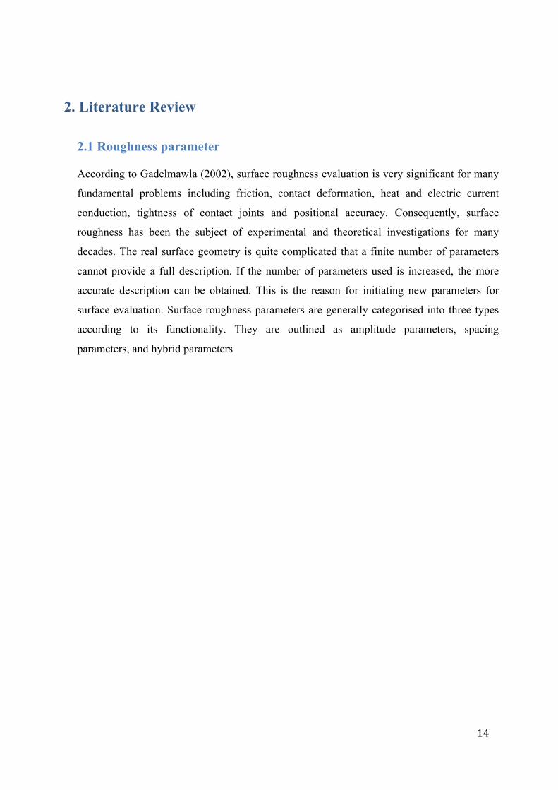
2. Literature Review
2.1 Roughness parameter
According to Gadelmawla (2002), surface roughness evaluation is very significant for many
fundamental problems including friction, contact deformation, heat and electric current
conduction, tightness of contact joints and positional accuracy. Consequently, surface
roughness has been the subject of experimental and theoretical investigations for many
decades. The real surface geometry is quite complicated that a finite number of parameters
cannot provide a full description. If the number of parameters used is increased, the more
accurate description can be obtained. This is the reason for initiating new parameters for
surface evaluation. Surface roughness parameters are generally categorised into three types
according to its functionality. They are outlined as amplitude parameters, spacing
parameters, and hybrid parameters

! 15!
2.1.1.The amplitude parameters The amplitude parameters are the most significant parameters to illustrate surface topography
(Gadelmawla, 2002). They are used to measure the vertical characteristics of the surface
deviations. It is given a brief description for each parameter.
Arithmetic average height (Ra)
Figure 1: Definition of arithmetic average height (Ra) (Gadelmawla, 2002)
The arithmetic average height parameter, also known as the centre line average (CLA), is
the most universally used roughness parameter for general quality control. It is expressed
as the average absolute deviation of the roughness irregularities from the mean line over
one sampling length as shown in Figure1. This parameter is easy to define, easy to
measure, and provides a good general description of height variations. It does not present
any information regarding the wavelength and it is not sensitive to small changes in
profile (Gadelmawla, 2002).

! 16!
Root mean square roughness (Rq)
Figure 2: Definition of the ten-point height parameter (Rz(iso),Rz(din) (Gadelmawla,
2002)
This parameter is also known as RMS. It signifies the standard deviation of the distribution
of surface heights, so it is an important parameter to describe the surface roughness by
statistical methods. This parameter is more delicate than the arithmetic average height (Ra) to
large deviation from the mean line (Gadelmawla, 2002).
Ten-point height (Rz)
This parameter is more complex to occasional high peaks or deep valleys than Ra. It is
described by two methods according to the definition system. The International ISO system
outlines this parameter as the difference in height between the average of the five highest
peaks and the five lowest valleys along the assessment length of the profile. Figure2 shows
the definition of the ten-point height parameter (Gadelmawla, 2002).

! 17!
Figure 3: Definition of the parameters Rp, Rv,Rpm,Rvm,Rt (Gadelmawla, 2002)
Maximum height of peaks (Rp)
Rp is outlined as the maximum height of the profile above the mean line within the
assessment length (Gadelmawla, 2002). In Figure3, Rp3 represents the Rp parameter.
Maximum depth of valleys (Rv)
According to Gadelmawla (2002), Rv is described as the maximum depth of the profile below
the mean line within the assessment length as shown in Figure 3. In the figure Rv4 represents
the Rv parameter.
Mean height of peaks (Rpm)
According to Gadelmawla (2002), Rpm is expressed as the mean of the maximum height of
peaks (Rp) obtained for each testing length of the assessment length as shown in Figure 3.
Mean depth of valleys (Rvm)
According to Gadelmawla (2002), Rvm is stated as the mean of the maximum depth of
valleys (Rv) obtained for each sampling length of the assessment length as shown in Figure 3.
Maximum height of the profile (Rt or Rmax)
This parameter is very sensitive to the high peaks or deep scratches. Rmax or Rt is described
as the vertical distance between the highest peak and the lowest valley along the assessment
length of the profile (Gadelmawla, 2002).

! 18!
Figure 4: Definition of the maximum peak to valley height parameters (Rti)
(Gadelmawla, 2002)
Maximum peak to valley height (Rti)
Rti is the vertical distance between the highest peak and the lowest valley for each sampling
length of the profile (Gadelmawla, 2002). As the assessment length is divided into five
sampling lengths, the maximum peak to valley height (Rti) can be defined, as shown in
Figure 4.
Mean of maximum peak to valley height (Rtm)
Rtm is outlined as the mean of all maximum peaks to valley heights obtained within the
assessment length of the profile (Gadelmawla, 2002).
Largest peak to valley height (Ry)
According to Gadelmawla (2002), this parameter is expressed as the largest value of the
maximum peak to valley height parameters (Rti) along the assessment length.
Profile solidity factor (k)
The profile solidity factor (k) is defined as the ratio between the maximum depth of valleys
and the maximum height of the profile (Gadelmawla, 2002).

! 19!
Skewness (Rsk)
Figure 5: Definition of skewness (Rsk) and the amplitude distribution curve
(Gadelmawla, 2002)
This parameter is a key factor in this project. According to Gadelmawla (2002), the skewness
of a profile is the third central moment of profile amplitude probability density function,
measured over the assessment length. It is used to measure the symmetry of the profile
regards to the mean line. This parameter is delicate to occasional deep valleys or high peaks.
A symmetrical height distribution with as many peaks as valleys has zero skewness. Profiles
with peaks removed or deep scratches have negative skewness. Profiles with valleys filled in
or high peaks have positive skewness as shown in Figure 5. The skewness parameter can be
used to distinguish between two profiles having the same Ra or Rq values but in different
shapes. The value of skewness depends on whether the bulk of the material of the sample is
above (negative skewed) or below (positive skewed) the mean line as shown in Figure 5. The
skewness parameter can be used to distinguish between surfaces, which have different shapes
and have the same value of Ra. In Figure 5, although the two profiles may have the same
value of Ra, they have different shapes.
! 20!
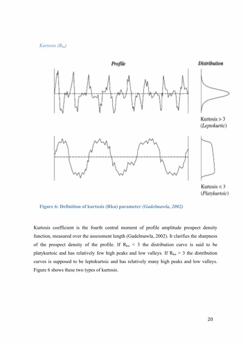
Kurtosis (Rku)
Figure 6: Definition of kurtosis (Rku) parameter (Gadelmawla, 2002)
Kurtosis coefficient is the fourth central moment of profile amplitude prospect density
function, measured over the assessment length (Gadelmawla, 2002). It clarifies the sharpness
of the prospect density of the profile. If Rku < 3 the distribution curve is said to be
platykurtoic and has relatively few high peaks and low valleys. If Rku > 3 the distribution
curves is supposed to be leptokurtoic and has relatively many high peaks and low valleys.
Figure 6 shows these two types of kurtosis.

! 21!
Figure 7: The ADF (Gadelmawla, 2002)
Amplitude density function (ADF)
The term amplitude density relates exactly to the term probability density in statistics. The
ADF signifies the distribution histogram of the profile heights (Gadelmawla, 2002). It can be
found by plotting the density of the profile heights on the horizontal axis and the profile
heights itself on the vertical axis as shown in Figure 7.

! 22!
Auto correlation function (ACF)
According to Gadelmawla (2002), the ACF labels the general dependence of the values of
the data at one position to their values at another position. It is considered as a very useful
approach for processing signals because it provides basic information about the relation
between the wavelength and the amplitude properties of the surface. The ACF can be studied
as a quantitative measure of the similarity between a laterally shifted and an unshifted
version of the profile. The ACF can be normalised to have a value of unity at a shift distance
of zero. This suppresses any amplitude information in the ACF but allows a better
comparison of the wavelength information in various profiles (Gadelmawla, 2002).

! 23!
Correlation length (b)
This parameter is used to describe the correlation characteristics of the ACF. It is outlined as
the shortest distance in which the value of the ACF drops to a certain fraction, usually 10%
of the zero shift value. Points on the surface profile that are separated by more than a
correlation length may be considered as uncorrelated portions of the surface characterised by
these points were produced by separate surface forming events. Correlation lengths may
range from the infinite correlation length for a perfectly periodic wavelength to zero for a
completely random waveform (Gadelmawla, 2002).
! 24!
2.1.2.The spacing parameters
According to Gadelmawla (2002), the spacing parameters are those, which measure the
horizontal characteristics of the surface deviations. The spacing parameters are solutions in
some manufacturing operations including pressing sheet steel. In such case, evaluating the
spacing parameters is necessary to obtain consistent lubrication when pressing the sheets, to
avoid scoring and to prevent the appearance of the surface texture on the final product. One
of the spacing parameter is the peak spacing, which can be an principal factor in the
performance of friction surfaces such as brake drums. By controlling the spacing parameters
it is possible to obtain better bounding of finishes, more uniform finish of plating and
painting. There are several types of spacing parameters.
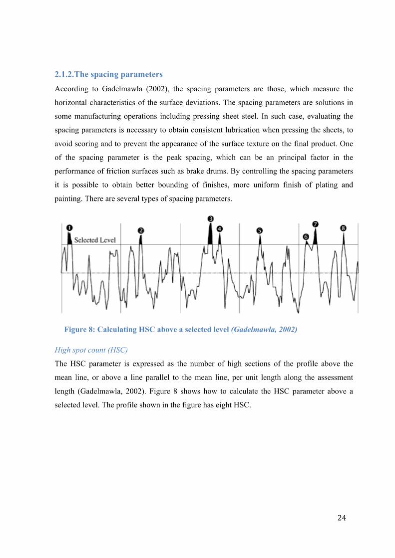
Figure 8: Calculating HSC above a selected level (Gadelmawla, 2002)
High spot count (HSC)
The HSC parameter is expressed as the number of high sections of the profile above the
mean line, or above a line parallel to the mean line, per unit length along the assessment
length (Gadelmawla, 2002). Figure 8 shows how to calculate the HSC parameter above a
selected level. The profile shown in the figure has eight HSC.
! 25!
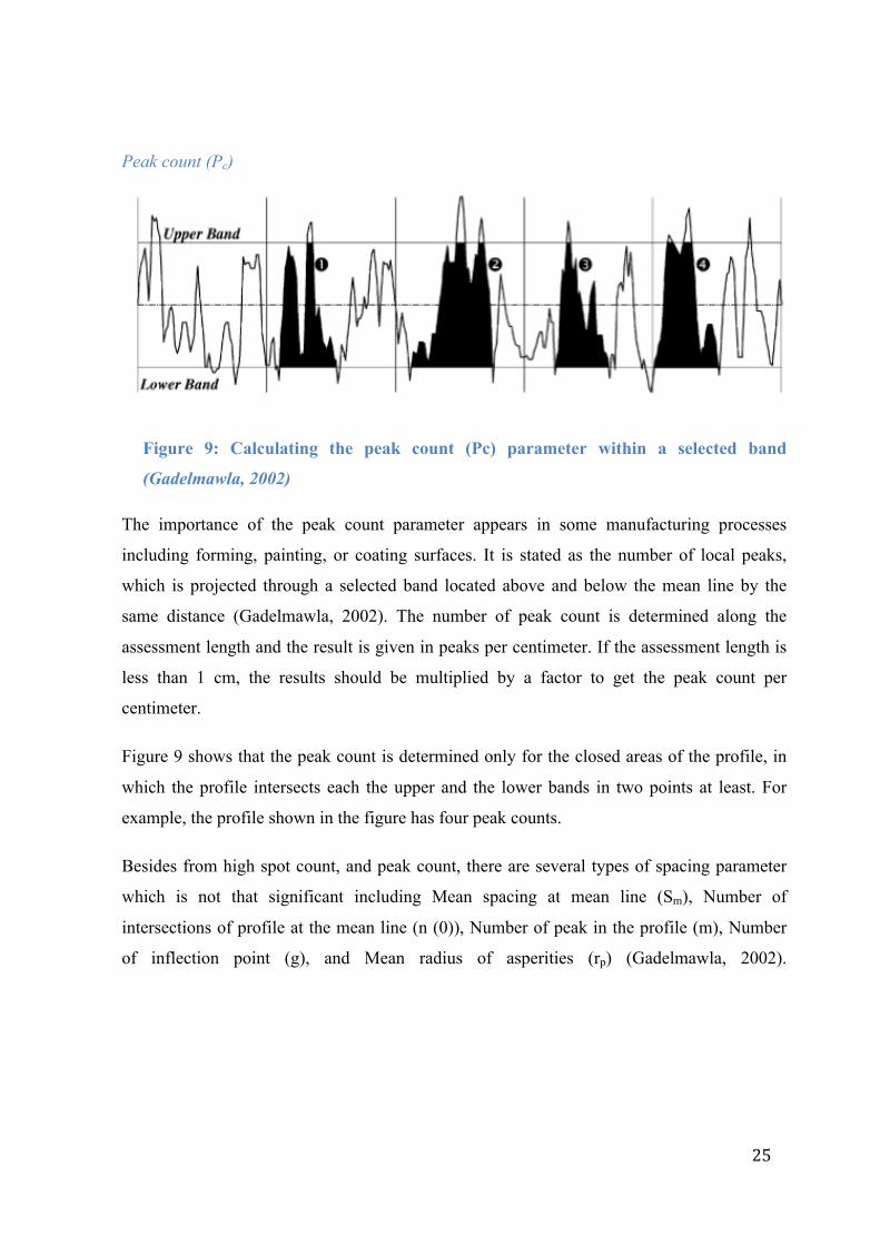
Peak count (Pc)
Figure 9: Calculating the peak count (Pc) parameter within a selected band
(Gadelmawla, 2002)
The importance of the peak count parameter appears in some manufacturing processes
including forming, painting, or coating surfaces. It is stated as the number of local peaks,
which is projected through a selected band located above and below the mean line by the
same distance (Gadelmawla, 2002). The number of peak count is determined along the
assessment length and the result is given in peaks per centimeter. If the assessment length is
less than 1 cm, the results should be multiplied by a factor to get the peak count per
centimeter.
Figure 9 shows that the peak count is determined only for the closed areas of the profile, in
which the profile intersects each the upper and the lower bands in two points at least. For
example, the profile shown in the figure has four peak counts.
Besides from high spot count, and peak count, there are several types of spacing parameter
which is not that significant including Mean spacing at mean line (Sm), Number of
intersections of profile at the mean line (n (0)), Number of peak in the profile (m), Number
of inflection point (g), and Mean radius of asperities (rp) (Gadelmawla, 2002).
! 26!
2.1.3.The hybrid parameters
According to Gadelmawla (2002), the hybrid property is a mixture of amplitude and spacing.
Any changes, which occur in either amplitude or spacing, could have effects on the hybrid
property. In tribology analysis, surface slope, surface curvature and developed interfacial
area are considered to be important factors, which influence the tribological properties of
surfaces. There are several types of hybrid parameter including Profile slope at mean line (!),
Mean slope at profile (Δ!), RMS slope at profile (Δ!), Average wavelength (!!), RMS
wavelength (!!), etc. However, these parameters are not taken into an account for this
project. Thus, it is not go in detail of them.

! 27!
2.2 Reynolds number
Chunhakham (2011) and Leepitakrat (2011) note that from the experiment of Reynolds in a
visual investigation of the flow of a liquid through a narrow tube, they observed that the air
density, viscosity and velocity of the fluid, and diameter of the tube had the effects in the
determining whether the flow would be laminar or turbulence. Then he could combine all
these parameters in one non-dimensional parameter, Reynolds number, and denoted by Re.
Re Vdρ=
µ (1)
(Ref: Fundamentals of Fluid mechanics, 5th, Bruce R. Munson et al., p. 518)
Where ρ is air density (kg/m3), V is fluid velocity (m/s), d is diameter (m), and µ is viscosity
of the fluid (N·s/m2).
The Reynolds number can be used to calculate the boundary layer of the flow. If Re is low,
boundary layer is likely to be laminar. If Re is moderately high, it is high prospect that the
boundary layer will be turbulence. In between the difference of the flow from laminar to
turbulence is called transition region.

! 28!
2.3 Critical Reynolds number
Clancy (1975) claims that drag force due to laminar boundary layers is much lower than the
drag due to the turbulent, thus it looks benefit to assure laminar flow past over the object
surface. However, it is difficult to keep the flow is laminar in high flow speed and non-linear
surface shape. If the flow is laminated over the objects but there are some separations occur,
drag force will be much higher than making the flow turbulence but still attaches the surface.
It is also the fact that laminar boundary layer tends to separate much more easily than the
turbulent flow. In high speed of flow and non-linear surface line, consequently, drag in
laminar flow will be likely to be higher than in transition to the turbulent because of the
separation. The prospect of occurrence of separation in turbulent flow is lower than laminar
since the delay of separation by higher energy of flow to attach the surface of the object,
resulting in reduction in drag.
Figure 10: Occurrence of separation (laminar boundary layer) (Chunhakham, 2011)
Figure 11: Occurrence of separation (turbulent boundary layer) (Chunhakham,
2011)

! 29!
Figure10 and Figure11 explain the flow separation past the circular cylinder (or sphere) in a
real fluid. Figure10 presents laminar flow past the cylinder in low Reynolds number. The
flow separates from the cylinder surface in the early position (front face of the cylinder),
providing a large region of dead air at the rear of the object. At high Reynolds number as
shown in Figure11, transition occurs early at the front face of the cylinder, leads to the
attachment of the flow to the surface until the points at rear of the surface. As the result, the
dead air section is lower than in laminar boundary layer case, providing much lower values
of drag. This phenomenon occurs quite swiftly when Re increased through the certain value,
‘Critical Reynolds number’. Consequently, the critical Reynolds number is a range of
Reynolds number that produces drag force and coefficient rapidly much lower than the
previous Reynolds number as shown in Figure 12
Figure 12: Illustration of critical Reynolds number (Chunhakham, 2011)

! 30!
2.4 Drag force and Drag coefficient
Munson et al. (2006), Chunakham (2011) and Leepitakrat (2011) describe that any object
moving through a fluid will experience a drag (D), a net force in the direction of flow due to
the pressure and shear force on the surface of the object. The equation of drag force can be
expressed as
! = ! !! !!!!!!!!! (2)
(Ref: Fundamentals of Fluid mechanics, 5th, Bruce R. Munson et al., p. 518)
Where !!is drag force, !! is air density, !! is flow velocity, !! is drag coefficient and !
is area.
Chunhakham (2011) asserts that the total drag force that acting on a bluff body can be
divided into two different parts, which are skin friction drag and pressure drag. The pressure
drag is a result of pressure difference between the high pressures in the front part of the body.
The difference of skin surfaces may cause the different drag force in the same air speed.
Rougher surface is more likely to produce the higher drag because of more separation of the
flow over the surface. Hoerner (1965) adds that the shape of the object also causes the
different drag force because of the difference of the pressures between front and rear faces.
The increase of drag due to the difference of pressure distribution, which is related to the
different value; higher different value leads to higher drag force.
!!!!"!#$ = !!!!!"#$$%"# !+ !!!!!"#$%#&' (3)
Where !!!!"!#$ = Drag coefficient of total drag, !!!!"#$$%"# = Drag coefficient of pressure
drag, !!!!"#$%#&' = Drag coefficient of skin friction drag
Chunhakham (2011) and Leepitakrat (2011) claims that the relative contribution of friction
drag and pressure drag vary on shape of the body and thickness. For bluff bodies including
cylinder, 90% of total drag comes from pressure drag. On the other hand, friction drag will
take the essential role on streamlined body.

! 31!
Figure 13: Comparison of drag forces from different shapes of objects and Reynolds
numbers (Chunhakham, 2011)
Figure13 demonstrates the relationship of the drag forces from different object shapes and
Reynolds numbers. The total drag force is the mixture of skin friction drag and pressure drag.
Nevertheless, drag force is likely from the effect of the difference of pressure distributions
except the airfoil shape. This may be because the area of surface contracting the airflow is
low while the difference of pressure distribution is relatively high. In the case of airfoil
shape, the contracted area is very large and the dead air at the back is very small, thus
mainstream of drag is from the skin friction drag (Leepitakrat, 2011).

! 32!
2.5 Effect of surface roughness
According to Kawamura and Takami (1986) and Chunhakham (2011), the effect of surface
roughness on the flow past a cylinder has been investigated experimentally. Some
experimental results from those experiments are used to compare the results in this
experiment. The surface roughness affects intensely in the transition in the boundary layer.
The small roughness on the surface can present the subcritical regime precipitately.
Methodical changes in the shapes and gradual displacement of the drag coefficient curves
towards the lower Reynolds number (Leepitakrat, 2011). These may be because of raising
the surface roughness. The roughness of surface will reduce the formation of the separation
bubble appearing at the rear of the object in smooth surface case. Therefore, those bubbles
are eliminated by the effect of roughness. Kawamura and Takami (1986) also states that the
surface roughness makes the critical Reynolds number lower that make the boundary thick
enough for practical computations and experiment.
An experiment of this investigation is the experiment of Achenbach (1971). In this well-
known experiment, three roughness values of the cylinder and smooth cylinder surface were
studied. This experiment was operated with a closed atmospheric circuit and alternatively
high-pressure wind tunnel. The tested cylinder had diameter of 150 mm with the length of
500 mm. This experiment also operated in the range of Reynolds numbers between 4x10⁴
and 3x10⁶. Figure14 shows the experimental result of Achenbach.

! 33!
Figure 14: Results of CD and Reynolds number without blockage correction
(Achenbach, 1971)
It is stated that in the subcritical flow regime, due to friction forces, the boundary layer
separates at the front portion of the circular cylinder with the laminar boundary layer
(Achenbach, 1971). The ratio of inertia forces to friction forces grows up with increasing
Reynolds number. The surface roughness will generate the additional energy to boundary
layer. From these two effects, thus, cause the boundary layer to attach to the surface for
longer distance. He adds that this moving of separation point to the back of cylinder reduces
the size of separation at the back, and as the result, the value of drag coefficient decreases.
Chunhakham (2011) and Leepitakrat (2011) declare that at the critical Reynolds number,
laminar separation and turbulence reattachment appear. For the case of smooth circular
cylinder in the large range of Reynolds number (3x10⁵ < Re < 1.5x10⁶), this phenomenon of
the separation bubble could be observed, but it is restricted for the rough surface cylinder
because of the narrow flow range.
They also add that the instant transition from laminar to turbulent flow could be observed in
the supercritical flow regime. When Reynolds number increases, the transition point moves
from back of the main cross-section to the point on the front face of the cylinder. As the

! 34!
result, the drag coefficient rises to reach the new higher value. Finally, the trans critical flow
regime is developed. In this regime, the turbulence is developed for the whole boundary layer
except the small region around the stagnation point. In this trans critical region, the total drag
coefficient has the constant value. This is the result from the idea that in trans critical flow
regime the magnitude of drag coefficient is only dependent on the effect of surface roughness
(Chunhakham, 2011).
Achenbach (1971) asserts that in the subcritical flow regime, due to friction forces, the
boundary layer separates at the front portion of the circular cylinder with the laminar
boundary layer. The ratio of inertia forces to friction forces grows up with increasing
Reynolds number. The surface roughness will generate the additional energy to boundary
layer. From these two effects, hence, cause the boundary layer to attach to the surface for
longer distance. This moving of separation point to the back of cylinder reduces the size of
separation at the back, and as the result, the value of drag coefficient decreases.
At the critical Reynolds number, laminar separation and turbulence reattachment appear. For
the case of smooth circular cylinder in the large range of Reynolds number (3x10⁵ < Re <
1.5x10⁶), this phenomenon of the separation bubble could be observed, but it is restricted for
the rough surface cylinder because of the narrow flow range.
The instant transition from laminar to turbulent flow could be observed in the supercritical
flow regime. When Reynolds number increases, the transition point moves from back of the
main cross-section to the point on the front face of the cylinder. As the result, the drag
coefficient rises to reach the new higher value. Finally, the transcritical flow regime is
developed. In this regime, the turbulence is developed for the entire boundary layer except
the small region around the stagnation point. In this transcritical region, the total drag
coefficient has the constant value. This is the result from the suggestion that in transcritical
flow regime the magnitude of drag coefficient is only dependent on the effect of surface
roughness.
Next!interesting!experiment!is!the!experiment!of!Achenbach!and!Heinecke!(1981).!This!
experiment!was!conducted!to!investigate!the!influence!of!the!surface!roughness!on!the!
vortex=shedding frequency in the wake of a single circular cylinder. The experiment was
operated in an atmospheric and a high-pressure wind tunnel with the range of Reynolds

! 35!
number 6x10³ to 6x10⁶. The experiment were tested with a smooth cylinder and rough
cylinder with relative roughness of ks/d = 75x10-5, 300x10-5, 900x10-5, and 3000x10-5.
Achenbach and Heinecke (1981) published the relationship between the dimensionless
roughness and the critical Reynolds number Recrit from the drag coefficient data of the
rough cylinders as following.
!Figure' 15' Drag' coefficient' of' single' cylinder' of' Achenbach' and' Heinecke's'
experiment'at'various'roughnesses'

! 36!
Another experiment is the investigation of the effect of surface skewness on the
postcritical and supercritical drag coefficient of the rough cylinders operated by Fuss
(2011). In this experiment, seven skewness roughness parameters Rsk: 0, +1, +2, +5, -1, -
2 and -5 and a smooth surface (Rsk = ±∞) were tested. The roughness elements have the
roughness height of 2 mm and supported with the base with thickness of 1.5 mm as shown
in Figure 16.
!Figure'16'Surface'profiles'in'the'experiment'by'Fuss'(2011)
In this experiment, two plates were attached at the end of the cylinder in order to reduce
the 3D effects. The wind speed was increased from 10 kph to 140 kph by increment of 10
kph. The results from this experiment were not necessary to be corrected with blockage
ratio because the blockage ratio is 1.7%, which is considered negligible.
The experimental results are shown in Figure 18. The magnitude of minimum drag
coefficient for the higher value of skewness (more value in positive) is higher than the
lower value of this roughness parameter. This means the higher positive skew is rougher
and higher negative skew is smoother.

! 37!
!Figure'17'Drag'coefficient'of'the'various'skewness'roughness'parameters'from'
Fuss''experiment'
!

! 38!
2.6 Flow past smooth circular cylinder
!Figure'18 Variation of drag coefficient with Reynolds number (Anderson, 1991)'
There are many researches and studies regards to the drag force in a range of Reynolds
number (Re). There are two main types of drag force including friction and stagnation
pressure (Hoerner, 1965). According to Chunhakham (2011), the different drag force
depends on skin surfaces in the same air speed. Rougher surface is more likely to create the
higher drag because of more separation of the flow over the surface. The shape of the object
causes the different drag force as well because of the pressure drag from the object itself. He
also declares that the pressure drag of this shape of object will be zero when it assumes to
have inviscid flow and incompressible flow over a circular cylinder. This is the result from
the same values of pressure distribution over the front and rear of the cylinder. Conversely,
the flow over a circular cylinder is different from the ideal case with no pressure drag. It will
have drag due to friction, and it is the function of Reynolds number. As Figure15 shows the
Variation of drag coefficient with Reynolds number based on experimental data, the values
of CD are very large compared to small Reynolds number Drag coefficient decreases
gradually until Reynolds number around 300,000, and then the value of CD is rapidly
dropped to near value of 0.3 to 0.6 at Reynolds number of 107. The reason of high CD at
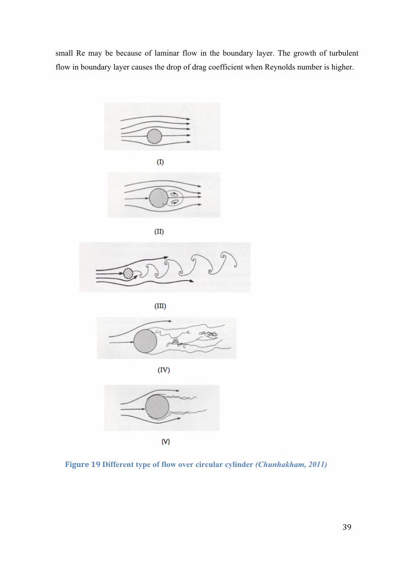
! 39!
small Re may be because of laminar flow in the boundary layer. The growth of turbulent
flow in boundary layer causes the drop of drag coefficient when Reynolds number is higher.
!Figure'19'Different type of flow over circular cylinder (Chunhakham, 2011)
! 40!
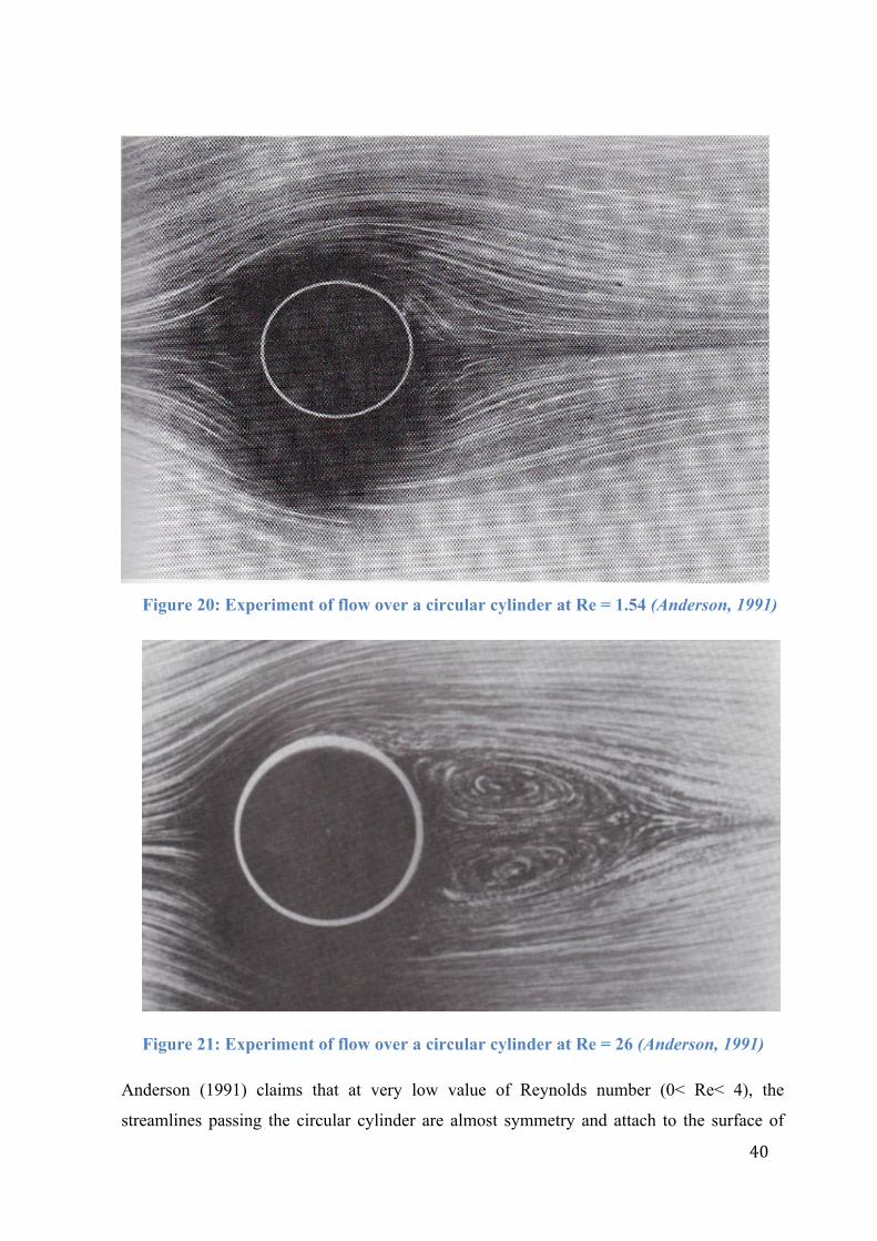
Figure 20: Experiment of flow over a circular cylinder at Re = 1.54 (Anderson, 1991)
Figure 21: Experiment of flow over a circular cylinder at Re = 26 (Anderson, 1991)
Anderson (1991) claims that at very low value of Reynolds number (0< Re< 4), the
streamlines passing the circular cylinder are almost symmetry and attach to the surface of

! 41!
cylinder as shown in Figure16 (I). This regime of viscous flow is called ‘Stokes flow’. Drag
force of this flow is due to the friction force; it is high value of CD because the surface that
touches the flow is large (about all elements on surface). Figure 19 is a figure of the
experiment of this type of flow where Re = 1.54. When the Reynolds number increases to a
range between 4 and 40, there are steady vortices at the back of the cylinder as shown in
Figure 16 (II). If the Re remains the same value, these vortices will stay at the same position
all the time.
Figure 22: The experiment of flow over a circular cylinder at Re = 140 (Anderson,
1991)
The experiment of this flow type where Re = 26 is shown in Figure 18 (Anderson, 1991). He
claims that since Re increases higher than 40, flow at the back of cylinder becomes unstable;
the vortices will be alternately shed from the body in an ordered fashion and flow
downstream as shown in Figure 16 (III). The alternatively shed vortex pattern as shown in
Figure 16 (III) is called a ‘Karman vortex street’.
The figure of the experiment of this flow type and also ‘Karman Vortex Street’ are shown in
Figure 19 (Re = 140). As increase of Reynolds number to be larger, the ‘Karman vortex
street’ becomes turbulent. The laminar boundary layer starts separating from the cylinder
surface on the forward face (about 80⁰ from the stagnation point) as shown in Figure 16 (IV)
Drag coefficient for this type of flow for 103 < Re < 3x10⁵ is constant as shown in Figure 15.

! 42!
The separation still occurs at the front face of cylinder but the free shear flow region in
previous Re region is replaced by transition to turbulent flow when the Reynolds number
increases from 3x10⁵ to 3x10⁶. Therefore the flows become reattached on the back of the
cylinder and separate again at about 120⁰ measured from the stagnation point as shown in
Figure 16 (V). The transitions to turbulent flow leads to reduction in pressure drag on the
circular cylinder; as the result, the CD will be reduced to the lowest values. The drag
coefficient will increase from the previous Reynolds number range when the Reynolds
number is higher than 3x10⁶. Moreover, the boundary layer transits directly to turbulence at
some point on the front face of the cylinder. However, the flow still fully attaches the circular
cylinder surface and separates at the back of the object around 120⁰ on the back face.
The separation points are moving closer to the top and bottom points of cylinder when the Re
keeps increasing. This impacts the waver wake, leading to higher value of pressure drag.
The flow over the cylinder is affected by the separation of the flow over the backward of the
object. This separation causes the disparity of the pressure distribution over the cylinder
surface between front and backsides of the circular cylinder. Figure 18 illustrates the
relationship the pressure distribution over the cylinder between the theoretic and experiment.
The theoretical result shows that there is no pressure difference between front and rear face
of the cylinder, so there is no drag due to the difference of the pressure distribution. In the
experiment with viscid and compressible flow, however, the pressure at front face of the
cylinder is higher than at the rearward face, leading to pressure drag, the difference of drag
between front and rear sides of the cylinder.

! 43!
!Figure'23'Comparison'of'pressure'distribution'over'the'cylinder'between'
theory'and'experiment
From Figure 18, drag coefficient of the cylinder at various Reynolds number can be drawn
roughly as shown in figure 23. Reynolds number can be divided into four regions as the
effects of Re on the drag coefficient. In the subcritical flow regime, there is a large range
of Re that CD is likely to be constant. After subcritical region, drag coefficient rapidly
drops with increasing Re. This region is called critical flow regime. Then CD starts
increasing with an increase of Re in supercritical flow regime. The last region is
transcritical region; drag coefficient of the cylinder is nearly constant again in this region
but with the lower values of CD. (Elmar Achenbach, 1971)

! 44!
!Figure'24'Flow'region'of'the'flow'past'over'the'circular'cylinder'(Achenbach,'
1971)'

! 45!
2.7 Flow past rough circular cylinder
According to B. R. Mudson Et al., the stream function and the velocity potential equation
are given by the combination of a doublet and uniform flow in the positive x direction.
The stream function;
! = !" sin! − ! !"#!! (4)
The velocity potential;
! = !" cos! − ! !"#!! (5)
For the stream function which is used to represent flow around a circular cylinder, the
value of ! = !"#$%&#% for!! = !, where ! is the radius of the cylinder. So the stream
function can be written as
! = ! − !!! ! sin!… (6)
(Ref: Fundamentals of Fluid mechanics, 5th, Bruce R. Munson et al.., p. 312)
It follows that ! = 0 for!! = ! if
! − !!! = 0 (7)
From the equation, doublet strength, K, is indicated it must be equal to Ua2. So, the
stream function of the flow around the circular cylinder can be expressed as
! = !" 1− !!!! sin! (8)
And the corresponding velocity potential is
! = !" 1− !!!! cos! (9)

! 46!
!Figure'25'The'flow'around'a'circular'cylinder
So, the velocity component can be obtained from the previous equations as
!! = !"!" =
!!!"!" = ! 1− !!
!! cos! (10)
And
!! = !!!"!" = − !"
!" = −! 1+ !!!! sin! (11)
(Ref: Fundamentals of Fluid mechanics, 5th, Bruce R. Munson et al.., p. 313)
On the surface of the cylinder (r = a), !! = 0
!!" = −2! sin! (12)
The maximum velocity occurs at the top and bottom of the cylinder (! = ±!/2) and has a
magnitude of twice the upstream velocity, U.
!
The pressure distribution of the cylinder surface can be found from the Bernoulli equation
which is written from a point far away from the cylinder where the pressure is !! and the
velocity is U so that
!! + !! !!
! = !! + !! !!!"
! (13)
Where

! 47!
!! = !ℎ!!!"#$%&'!!"#$$%"#
Since !!" = −2! sin! and elevation change are neglected, the surface pressure can be
express as
!! = !! + !! !!
!(1− 4 sin! !) (14)
!Figure'26'A'comparison'of'theory'pressure'distribution'of'surface'of'a'circular'
cylinder'with'typical'experimental'distribution
A comparison of the theoretical, symmetrical pressure distribution express in
dimensionless form with a typical measured distribution is shown in Figure 21. The figure
clearly reveals that only on the upstream part of the cylinder is there approximate
agreement between the potential flow and the experiment results Because of the viscous
boundary layer that develop on the cylinder, leading to the large difference between the
theoretical, frictionless fluid solution and the experiment result on the downstream side of
the cylinder.

! 48!
!Figure'27'The'notation'for'determining'lifts'and'drags'on'a'circular'cylinder
The resultant force (per unit length) develop on the cylinder can be determined by
integrating the pressure over the surface. From Figure 20, it can be seen that
!! = − !! cos! !!!"!!! (15)
!! = − !! sin θ!!!"!!! (16)
Where
!! = !ℎ!!!"#$! !"#$%!!"#"$$%$!!"!!"#$%&"'(!!"!!ℎ!!!"#$%&'!!"#$
!!= !ℎ!!!"#$! !"#$%!!"#!"$%&'()*#!!"!!"!!"#$%&"'(!!"!!ℎ!!!"#$%&'!!"#$
(Ref: Fundamentals of Fluid mechanics, 5th, Bruce R. Munson et al.., p. 314)
!

! 49!
2.8 Blockage effect
Leepitakrat (2011) clarified that blockage ratio (S/C) is defined the ration of the effective
area of the model that normal to the wind direction to the cross-sectional area of wind
tunnel. Nevertheless, there is a little work that concerned this effect even at the relatively
high blockage ratios. He added that many researchers have attempted to avoid this effect
by adjusting the tunnel test section in some ways. Increase of the blockage ratio leads to
the moving of separated shear towards to the wake centre line. There is an agreement that
for the blockage ratios of up to 10% are acceptable (Leepitakrat (2011).

! 50!
3. Methodology
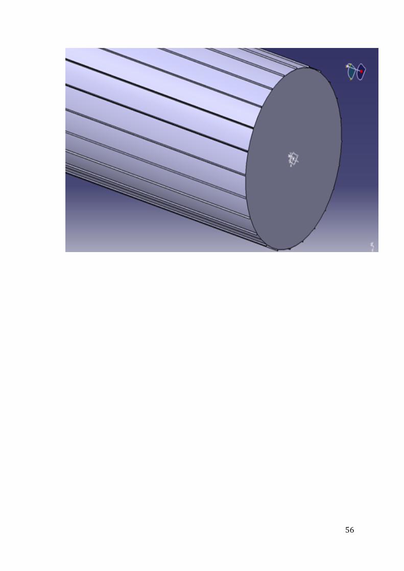
3.1 Testing model design
In the experiment, eight roughness surfaces of 310mm. × 300mm. with various profile of the
Rsk of ±∞, 0, +1, +2, +5, -1, -2 and -5 as shown in Figure 20 are experimented. The
roughness specimens have the roughness height of 1 mm and supported with the base with
thickness of 1 mm. The specimen sheets are made from the material named “TP930”, a
flexible polymeric rapid prototyping material (Fuss, 2011). The models are bended into
cylinder shape when experimenting. The reason of using circular cylinder in the experiment
is to complete the flow in high Reynolds number.
Figure 28: Surface profile and skewness numbers (Fuss, 2011)

! 51!
!
!Figure'29'Specimen'sheets'with'various'skewness'numbers'

! 52!
!Figure'30'Specimen'sheet'

! 53!
!'
Figure'31'Specimen'sheet
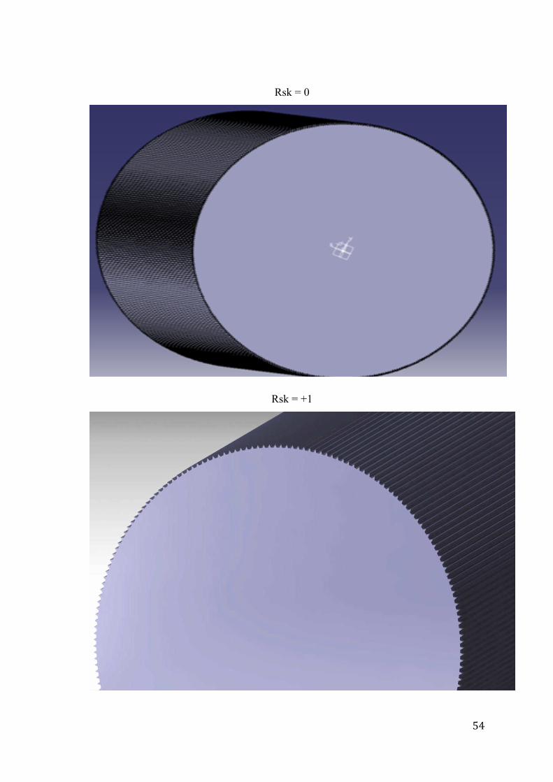
! 54!
Rsk = 0
Rsk = +1

! 55!
Rsk = +2
Rsk = +5
! 56!

! 57!
Rsk = -1
Rsk = -2

! 58!
Rsk = -5
Rsk = ∞
!Figure 32 Cylinderical surface profiles and skewness numbers (Chunhakham, 2011)

! 59!
3.2 Test rig
!Figure 33: The test rigs in a front view and oblique view in respectively (Fuss, 2011)
The TP930 test sheets will be covered around the cylinder with the ridges supported in
span wise direction (Fuss, 2011). The sheets is attached to the surface of the cylinder by
glue and also secured with tape at the seams (stagnation points) and the cylinder end
plates as shown in Figure 29. Since the supporting base layer of 1 mm thickness of each
TP930 test sheet, the relative surface roughness was 0.9%. According to Fuss (2011), The
test rig in Figure21 is designed for wind tunnel testing including a horizontal cylinder
located in the centre of the tunnel’s cross section. He adds that the wind speed was
boosted in increments of 10 kph from 20 kph to 140 kph, and at each velocity step, the
wind speed was retained constant for 10 s. The data were recorded with Kistler Bioware
(Kistler, Winterthur, Switzerland) at 20 Hz. (Fuss, 2011). By analysis, the horizontal force
data were tared, by subtracting the test rig’s drag force (without cylinder) from the
experimental data (cylinder with TP930 test sheets). The blockage ratio of 1.17% was
neglected and thus not corrected. Then the data is plotted, and the segments of constant
wind speed were known. After that, the average drag force calculated for each velocity
step. The drag forces and wind speeds were changed to drag coefficient and Reynolds
number (Fuss, 2011).

! 60!
3.3. Wind tunnel
This experiment will be conducted by using RMIT University Wind tunnel. It is secure
return circuit wind tunnel. The maximum speed of the wind in the tunnel is approximately
145 km/h or 40.3 m/s. the test section is 3 m × 2 m cross-section and long 9 m. The wind
speed will be measured by anemometer that was build from electric motor and blade.
Figure 34: The test section of wind tunnel (Chunakham, 2011)

! 61!
3.4 Cylinder model
A wood cylinder model with diameter of 125 mm and length of 310 mm will be used in
order to examine the aerodynamic properties of the garments. Two circular side plates
with three times of the cylinder model size will be attached at both end of the cylinder in
order to simulate 2D flow. The reason is that the cylinder model length is finite, so when
the flow passes, circulation will occur at both model’s ends. This circulation will disturb
the flow and lead to error. Both cylinder model and side plates will be mounted with the
testing base
. !
Figure'35'Cylinder'model'(Leepitakrat,'2011)

! 62!
!
'
Figure'36'Cylinder'model
!Figure'37'Slide'plate

! 63!
3.5 Testing base
The testing base is equipment that will be used to hold the cylinder model on the
horizontal direction during the experiment. It was designed to receive vibration from
flutter, and made from metal.
!Figure'38'Testing'base'before'reinforcement

! 64!
!Figure'39'Test'rig'being'reinforcement'and'installed'cylinder'
The figure 39 shows the testing base before reinforced. It was tested in the wind tunnel
and vibrated at high air speed. Because of this, two plates with the same materials
reinforce it. The anemometer will be mounted at one side of the testing base.

! 65!
!Figure'40'Testing'base'model'after'reinforced'(Chunhakham,'2011)

! 66!
3.5 Force balance
!Figure'41'Force'balance'(Chunhakham,'2011)'
In the experiment, drag, lift, side forces and yaw, pitch, roll moments will be monitored
and recorded. The most important parameter is drag force because the flow is assumed to
be parallel to the textile positioning and there is no need to adjust the turntable under the
wind tunnel to change the angle of attack. Other parameters except drag force will not
change much.

! 67!
3.5 Anemometer
An anemometer is the equipment that is used to measure air speed. It is required in order
to calibrate air velocity inside the wind tunnel. This will help reducing error caused by the
wind tunnel. The velocity will be shown in the display in m/s.
!Figure'42'Anemometer'(Chunhakham,2011)'

! 68!
3.7. Calculation of Ftared
In order to get the real result from the experiment, the forces in the correct direction are
used to calculate, as there are six forces that can measure in the wind tunnel. There are
five main variables related to time that use to get average Cd and Re. First variable is
Force in horizontal direction or Fy. It can be obtained in the experiment. Second,
equivalent speed or veq is also attained from experiment. Third, Fy(tared) is calculated
from Fy or Fy(untared) Begin with using equation of Cd(equivalent) which is
Cd(equivalent) = -5.983482221E-005 x v(m/s) + 0.02886483494
From three experiment, the Fy(tared) can be plotted to the graph below
0 10 20 30 40v (m/s)
0
0.01
0.02
0.03
0.04
2*rh
o*A
d
!

! 69!
The graph is plotted from 2 x rho x Ad by v (m/s) represents three Fy(tared) and the
average Fy(tared). From these graphs, there will be obtained three equations which are
Equation Y = -5.983482221E-005 x X + 0.02886483494
Equation Y = -5.350914793E-005 x X + 0.02900245644
Equation Y = -9.23545689E-005 x X + 0.03075105637
For X = 7 to 36 (m/s)
Then, it is attained average equation of the three equation.
The gradient of equation = -6.856617968E-005
The intercept = 0.02953944925
Thus, equation Y = -6.856617968E-005 x v (m/s) + 0.02953944925
Finally, the of Fy(tared) = of Fy(untared) – v2 (m/s) x (-6.856617968E-005* v(m/s) +
0.02953944925).
Forth, v (m/s) = !!"#$%
!.!"!#$%$!&
Last variable is constant which is rho. It is equal to 1.2054
When five variables are obtained, Cd and Re can be acquired.
Cd = !!"#$%!!"!!!!!".!"#$ , where 25.8065 is AxD of cylinder
Re = !.!"#!!!!!!!.!!!!"#$
The last step for plotting graph is to use average of Cd and Re

! 70!
4. Experimental result and Discussion
Experimental result
Rsk = ∞
Regarding the above graph, it indicates the drag coefficient on skewness surface, which
has skewness number equals to infinity versus Reynolds number. The trend of this graph
is similar to the graph based on the experimental data given in Anderson (1991). In other
words, it can be said that skewness number, which equals to infinity is the same as smooth
surface. There is a dramatically decrease of drag coefficient along the graph, however, it
seems constant in the end. Due to the fact that coefficient drag will decrease at higher
velocity, thus, the result looks quite good as it is expected; yet it should shift a bit to the
right
.
0!
0.2!
0.4!
0.6!
0.8!
1!
1.2!
0! 50000! 100000! 150000! 200000! 250000! 300000!
Reynolds number
Cd
! 71!
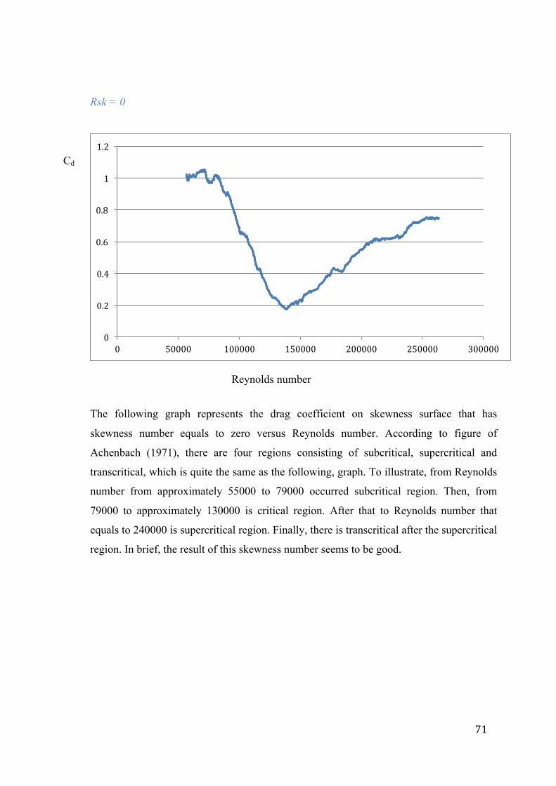
Rsk = 0
The following graph represents the drag coefficient on skewness surface that has
skewness number equals to zero versus Reynolds number. According to figure of
Achenbach (1971), there are four regions consisting of subcritical, supercritical and
transcritical, which is quite the same as the following, graph. To illustrate, from Reynolds
number from approximately 55000 to 79000 occurred subcritical region. Then, from
79000 to approximately 130000 is critical region. After that to Reynolds number that
equals to 240000 is supercritical region. Finally, there is transcritical after the supercritical
region. In brief, the result of this skewness number seems to be good.
0!
0.2!
0.4!
0.6!
0.8!
1!
1.2!
0! 50000! 100000! 150000! 200000! 250000! 300000!
Reynolds number
Cd

! 72!
Rsk = 1
Regards to the following graph, it presents the drag coefficient on skewness surface,
which has skewness number equals to positive one versus Reynolds number. Despite it
shows four regions in this graph including subcritical region, critical region, supercritical
region, and transcritical region, the graph is not as expected. The graph should be shifted
down a bit by the critical Reynolds number should plunge to drag coefficient equals to
0.2.
0!
0.2!
0.4!
0.6!
0.8!
1!
1.2!
0! 50000! 100000! 150000! 200000! 250000! 300000!
Reynolds number
Cd

! 73!
Rsk = 2
The following graph represents the drag coefficient on skewness surface that has
skewness number equals to positive two versus Reynolds number. The trend of this graph
looks good compared to the previous experiment of Fuss (2011).
0!
0.1!
0.2!
0.3!
0.4!
0.5!
0.6!
0.7!
0.8!
0.9!
1!
0! 50000! 100000! 150000! 200000! 250000!
Reynolds number
Cd

! 74!
Rsk = 5
According to the above graph, it represents the drag coefficient on skewness surface that
has skewness number equals to positive five versus Reynolds number. The trend of this
graph looks good compared to the previous experiment of Fuss (2011).
0!
0.1!
0.2!
0.3!
0.4!
0.5!
0.6!
0.7!
0.8!
0! 50000! 100000! 150000! 200000! 250000! 300000!
Reynolds number
Cd

! 75!
Rsk = -1
Regarding the following graph, it presents the drag coefficient on skewness surface,
which has skewness number equals to negative one versus Reynolds number. It is
different as it is expected. Since the subcritical region should plunge to approximate 0.2 at
Reynolds number equals to 150000. This may result from the error of the average in many
experiments. As there may be an error in some experiment, it can change the trend of the
graph.
0!
0.2!
0.4!
0.6!
0.8!
1!
1.2!
1.4!
1.6!
1.8!
0! 50000! 100000! 150000! 200000! 250000! 300000!
Reynolds number
Cd

! 76!
Rsk = -2
The graph represents the drag coefficient on skewness surface that has skewness number
equals to negative two versus Reynolds number. According to figure of Achenbach
(1971), there are four regions consisting of subcritical, supercritical and transcritical,
which is quite the same as the following, graph. To illustrate, from Reynolds number from
approximately 50000 to 17000 occurred subcritical region. Then, at Reynolds number
equals to approximately 175000 is critical Reynolds number. After that to Reynolds
number that equals to 200000 is supercritical region. Finally, there is transcritical after the
supercritical region. In brief, the result of this skewness number seems to be good.
0!
0.2!
0.4!
0.6!
0.8!
1!
1.2!
0! 50000! 100000! 150000! 200000! 250000! 300000!
Reynolds number
Cd

! 77!
Rsk = -5
!!
!
!
According to the above graph, it represents the drag coefficient on skewness surface that
has skewness number equals to negative five versus Reynolds number. The trend of this
graph looks good compared to the previous experiment of Fuss (2011). However, the
graph should be shift downward as skewness number of zero.!
0!
0.2!
0.4!
0.6!
0.8!
1!
1.2!
1.4!
0! 50000! 100000! 150000! 200000! 250000! 300000! 350000!
Reynolds number
Cd

! 78!
!
Discussion
!!
!
From the purpose of this experiment is to study the effect of various surfaces skewness on
a critical Reynolds number. There are eight skewness numbers, which is tested in the
wind tunnel. There are several experiments of some skewness number that have satisfied
result and including skewness number equals to infinity, zero, positive two, positive five,
negative two, negative five. Other skewness number that have different graph trend may
be occur from an average method. Since there may be some experiment that error, it affect
significantly to the average graph.
0!
0.2!
0.4!
0.6!
0.8!
1!
1.2!
1.4!
1.6!
1.8!
0! 50000! 100000! 150000! 200000! 250000! 300000! 350000!
AVERAGE'skewness'
avginWi!
avgneg1!
avgneg2!
avgneg5!
avgpos1!
avgpos2!
avgpos5!
avgzero!
Reynolds number
Cd

! 79!
!
!
5. Conclusion
The purpose of this project is to study the effect of surface skewness on critical Reynolds
number and also discuss and analyse the data from the experiment. In this semester, the main
tasks are to study thee theory of the roughness surface, do the experiment in the wind tunnel,
and analyse the data. However, it is not be able to do the experiment since the manufacturing
of the specimen is not be done in this semester, thus the experiment will be conducted in next
semester and also the research and development will be accomplished.
In the literature review, some studies, which has similar or same objective will be taken into
an account. Some assumption and errors from the studies will be a guideline for research and
development later on. According to the experiment by Fuss (2011), the critical Reynolds
number is decreased by surface roughness. From these experiments also show that the
minimum drag coefficient at critical Reynolds number of the higher roughness is higher
compared to the lower surface roughness values. This is the result from the effect of surface
roughness. The higher magnitude of surface roughness will cause more friction drag than the
smoother surface.
For the experiment that investigated the effect of skewness roughness parameter conducted
by Fuss (2011), the results show that the higher value of skewness (more positive) means
rougher whilst the lower value of this roughness parameter (more negative) will acts as the
smoother surface. The effect of skewness surface on critical Reynolds number number can be
summarised. The higher skewness value will have the lower critical Reynolds number
compared to lower skewness value because of the results of skewness effect from Fuss
(2011). Moreover, drag coefficient at the critical Reynolds number will be higher in more
positive skewness value.
From the experimental result, there are some satisfied result and result that different from
theory. The error would come from the averaging method of graph. There may be some
graphs that have an error so it affects the average graph.

! 80!
6. Recommendation for future studies
From! the! experience! in! this! project! regarding! the! effect! of! surface! skewness! on!
critical! Reynolds! number,! several! recommendations! for! the! future! studies! can! be!
drawn.!
First,! in! the!experiment,! it!must!be!ensured! that! the! specimen!plate! is! stick! to! the!
cylinder!completely,!unless!fluttered!may!occur.!
Second,! there!might! be! error! on! the! averaging! graph!method.! To! reduce! an! error,!
more!tests!for!each!specimen!could!be!conducted.!
Third, the range of Reynolds number will be effective from the velocity of 7 m/s to 36
m/s, unless there will be a turning point which may lead to an error.

! 81!
Reference
Achenbach, E and Heinecke, E, 1981, on vortex shedding from smooth and rough cylinders
in the range of Reynolds numbers 6×10³ to 5×10⁶, J. Fluid Mechanics Vol. 109, pp.239-251,
Great Britain.
Achenbach, E, 1971, Influence of surface roughness on the cross-flow around a cylinder, J.
Fluid Mechanics vol. 46, part 2, pp. 321 – 335.
Anderson, D, J Jr., 1991, Fundamental of Aerodynamics, 2nd edition
Chunakham, P, 2011, Effect of surface skewness on critical Reynolds number, Final year
project, RMIT University
Flitney, R, K and Melvin, B, W, 2007, Seals and sealing handbook 5th edition, ELSEVIER,
Amsterdam, Netherland.
Fuss, F, K, 2011, the effect of surface skewness on the super/postcritical coefficient of drag
roughness cylinders, ELSEVIE
Gadelmawla, E, S M. M. Koura, T. M. A. Maksoud, 2002, Roughness parameters, Journal of
materials processing technology vol. 123, pp. 133-145.
Hoerner, S, F, 1965, FLUID-DYNAMIC Drag, pressure drag, Chapter III.
Thomas, T, R, Characterization of surface roughness, 1981, Precision Engineering, IPC
Business Press, pp. 97 – 104.
Leepitakrat, Y, 2011, Effect of surface skewness on critical Reynolds number, Final year
project, RMIT University
Munson, B, R, 2006, Fundamental of Fluid Mechanics, John Wiley and Son, Inc., pp. 310-
334

! 82!
Nakamura, Y and Tomonari, Y 1982, the effects of surface roughness on flow past circular
cylindrical at high Reynolds number, J. Fluid Mechanics vol. 123, pp. 363 – 378.
Zipin, R, B, 1981, the height sensitive surface roughness parameter, application of surface
science 9, pp. 226 – 287, North-Holland Publishing Company, Netherland.