The economic significance of conditional skewness in index option markets

The authors thank the editor, Robert I. Webb, an anonymous referee, Phelim Boyle, Jin-Chuan Duan, SteveFiglewski, Mark Shackleton, Rangarajan Sundaram, Raul Susmel, and Ken Vetzal for their helpful commentsthat have significantly improved the article. We also thank participants at the European Finance AssociationMeetings 2003, Glasgow, Midwest Finance Association Meetings 2003, St. Louis, Fifth Annual FinancialEconometrics Conference 2003, University of Waterloo, Northern Finance Association Meetings 2002,Banff, the UTI Sixth Capital Markets Conference 2002, Mumbai, the CGA Conference 2002, University ofManitoba, and the University of Houston for their suggestions. This article received the Best Paper Award(Derivatives and Risk Management Category) at the Midwest Finance Association Meetings 2003.

*Correspondence author, Financial Services Research Centre, School of Business and Economics, WilfridLaurier University, Waterloo, Ontario, Canada N2L 3C5. Tel: �1-519-884-0710x2187, Fax: �1-519-884-0201,e-mail: [email protected], [email protected]

Received March 2007; Accepted March 2009

■ Ranjini Jha is at the School of Accounting and Finance, University of Waterloo, Waterloo,Ontario, Canada.

■ Madhu Kalimipalli is at the Financial Services Research Centre, School of Business andEconomics, Wilfrid Laurier University, Waterloo, Ontario, Canada.

The Journal of Futures Markets, Vol. 00, No. 0, 1–29 (2009)© 2009 Wiley Periodicals, Inc.Published online in Wiley InterScience (www.interscience.wiley.com).DOI: 10.1002/fut.20414

THE ECONOMIC SIGNIFICANCE

OF CONDITIONAL SKEWNESS IN

INDEX OPTION MARKETS

RANJINI JHAMADHU KALIMIPALLI*

This study examines whether conditional skewness forecasts of the underlyingasset returns can be used to trade profitably in the index options market. Theresults indicate that a more general skewness-based option-pricing model cangenerate better trading performance for strip and strap trades. The results showthat conditional skewness model forecasts, when combined with forward-lookingoption implied volatilities, can significantly improve the performance of skewness-based trades but trading costs considerably weaken the profitability of indexoption strategies. © 2009 Wiley Periodicals, Inc. Jrl Fut Mark

2 Jha and Kalimipalli

Journal of Futures Markets DOI: 10.1002/fut

INTRODUCTION

Skewness in asset returns can have significant impact on portfolio allocationand option trading decisions. Patton (2004) shows that for investors with noshort-sales constraints (such as hedge funds), knowledge of higher conditionalmoments and asymmetric dependence leads to portfolio gains that can be eco-nomically and statistically significant. The objective of this study is to investi-gate whether conditional skewness forecasts generated by time-series modelscan be used to profitably trade in S&P 500 index (SPX) options, and whetherthere is an incremental benefit to option traders in using skewness forecasts inaddition to the conditional volatility forecasts.

Economic models involving effects of the higher-order return momentshave received widespread attention in the literature (for example, Dittmar,2002; Giot & Laurent, 2003; Jondeau & Rockinger, 2003; Patton, 2004).Hansen (1994) provides a conditional skewness model, which is based on askewed central Student’s-t distribution, and Harvey and Siddique (1999) pro-pose a skewness model based on a non-central conditional t distribution.Harvey and Siddique (2000) show that skewness effects are important in addi-tion to size and book-to-market effects, in order to explain the cross section ofequity returns. Bekaert and Wu (2000) examine the role of volatility feedbackand leverage effects in explaining skewness.

Extant studies have proposed alternative model specifications to explainthe negative skewness in the option implied risk-neutral distributions. Forexample, Heston (1993) and Nandi (1998) examine the role of stochasticvolatility (SV) on option pricing. Bates (1996, 2000), Bakshi, Cao, and Chen(1997), Ait-Sahalia, Wang, and Yared (2001), and Pan (2002) develop modelsthat incorporate SV and time-varying jumps in returns.1 Eraker, Johannes, andPolson (2003) argue that SV or jumps in returns alone are inadequate specifi-cations, and that jumps in volatility are additionally needed to explain theunderlying smile biases. Coval and Shumway (2001) show that negative optionreturns earned by zero-beta at-the-money (ATM) straddles imply that systemat-ic SV is a priced factor. Several studies have also examined the role of deter-ministic volatility models in explaining the volatility skews and out-of-sampleoption pricing and hedging (e.g., Dumas, Fleming, and Whaley, 1997; Buraschiand Jackwerth, 2001; and Hull and Suo, 2002).

Further work has examined the impact of non-normal distributions onoption pricing and hedging. Lehnert (2003) and Christoffersen, Heston, andJacobs (2006) explore the effect of skewness on option valuation. Lim,Martin, and Martin (2005, 2006) show that pricing higher-order moments1Additional references include Das and Sundaram (1999), Chernov and Ghysels (2000), Heston and Nandi(2000), Bakshi, Kapadia, and Madan (2003), Jones (2003), Eraker (2004), Constantinides, Jackwerth, andPerrakis (2009), and Carr and Wu (2003, 2007).

Economic Significance of Conditional Skewness 3


and time-varying volatility yields improvements in the pricing of options. Theseauthors compare the relative effectiveness of modeling risk-neutral distributionsusing (a) generalized Student’s-t (GST) distribution, (b) semi-non-parametric(SNP) distribution (also employed by Corrado & Su, 1996, 1997), and (c) mix-ture of log-normal distributions and find that the GST modeling framework issuperior to the alternative SNP and log-normal mixture models in capturing thevolatility skew associated with the Black–Scholes model. Martin, Forbes, andMartin (2005) employ Bayesian inference methods to compare option pricesbased on alternative conditional volatility, skewness, and kurtosis specifications.

Dennis and Mayhew (2002) study skewness of individual equity optionsand show that liquidity and firm size help explain the cross-sectional differ-ences in skew. Bollen and Whaley (2004) provide an explanation for theimplied volatility (IV) smirk based on excess buying pressure for out-of-the-money (OTM) puts.

Coval and Shumway (2001, p. 984) note that as option values are nonlin-ear functions of the underlying asset’s values, option returns are sensitive tohigher moments of the underlying asset’s returns. As the risk-neutral distribu-tion is jointly determined by the empirical distribution and the aggregate riskaversion measure (Jackwerth, 2000), this study examines to what extent thetime-varying skewness impacts returns from the option trading strategies.

This article focuses on option trading because it provides a robust bench-mark to evaluate the economic performance of alternative skewness forecasts.Profits from option trading depend upon the underlying market risks (such asdelta, gamma, and vega risks), market liquidity, implicit bid–ask spreads, com-mission costs, and margin requirements. A superior model based on an out-of-sample statistical analysis may not necessarily perform well in trading due tomarket imperfections. For example, Figlewski (1989) shows that the presenceof market imperfections such as imperfect volatility estimates, transactioncosts, indivisibilities in contract size, and discrete rebalancing can set limits toperfect arbitrage in option markets. Santa-Clara and Saretto (2005), using anin-sample analysis, examine various strategies including naked and coveredpositions in options, straddles, strangles, and calendar spreads, and find sup-port for mispricing in the options markets, which cannot be arbitraged awaydue to high trading costs and margin requirements.

In this study, an extensive in-sample and out-of-sample evaluation of alter-native conditional volatility and skewness models is performed followed by aninvestigation of its implications for different option trading strategies. Two typesof trades are employed: volatility trades that consist of trades in ATM straddlesand skewness trades that involve trading ATM straddles, strips, and straps.

The study’s principal finding is that a more general skewness-based option-pricing model (Corrado & Su, 1996, 1997) can generate better trading



performance for strip and strap trades. The results show that conditional skew-ness model (Hansen, 1994) forecasts, when combined with option IV fore-casts, can significantly improve the performance of skewness-based trades.Trading costs (arising from bid–ask spreads) eliminate the profitability ofoption strategies. The results are consistent with Santa-Clara and Saretto(2005), who find that the high returns in option strategies (documented instudies such as Coval & Shumway, 2001) do not necessarily translate into prof-itable strategies after considering trading costs.

The rest of the article is organized as follows: The second section describesthe data and summary statistics; the third section discusses the performance ofdifferent time-series models. The fourth section presents the results of thetrading strategies; the fifth section presents the robustness tests, and the finalsection presents the conclusions.

DATA AND SUMMARY STATISTICS

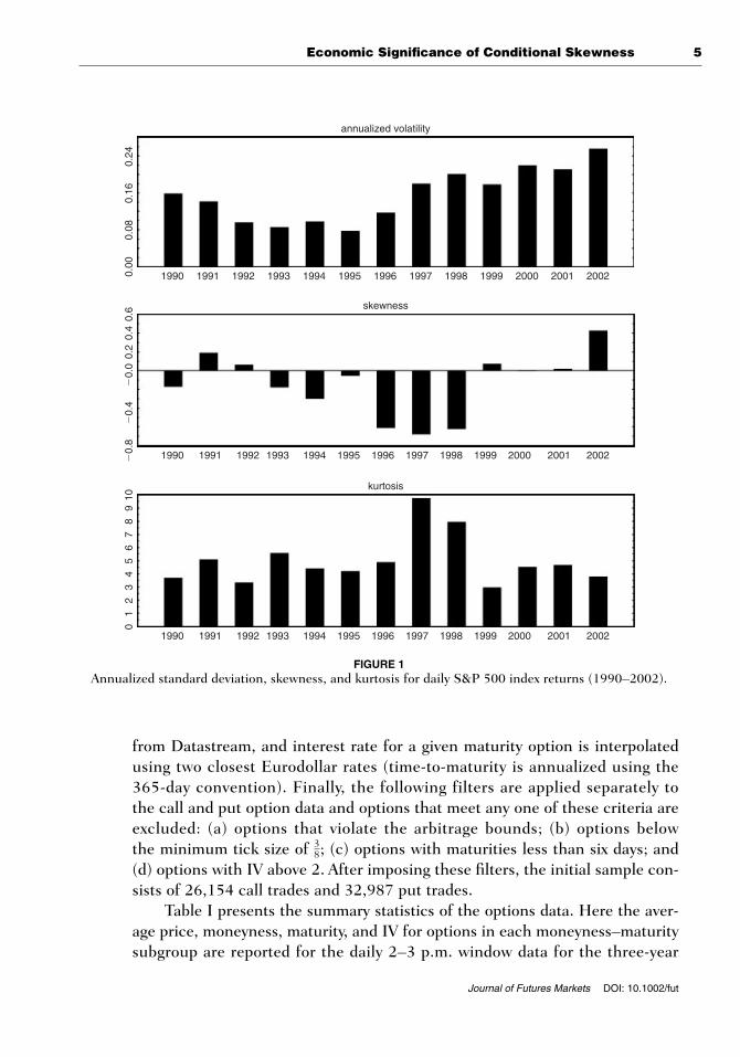
Daily SPX data for the period 1990–2002 are obtained from the DatastreamInternational database. Figure 1 plots the annualized unconditional or rawvolatility (standard deviation), skewness, and kurtosis values each year for thedaily return data over the sample period. Inspection of the data reveals thatvolatility has been steadily rising since the mid-1990s. Market volatility hasbeen high during periods of market shocks, such as wars, financial crises, ortechnology bubbles. High-volatility periods generally correspond to periods ofnegative skewness and high kurtosis. Periods of negative skewness seem tohave much larger skewness magnitude compared to positive news periods.

Intra-day SPX options along with intra-day spot data for the option tradingexercises are used for the analysis. SPX options are widely traded, being thesecond most liquid options in terms of trading volume and most liquid in termsof open interest in the United States (for earlier applications, see Bakshi et al.,1997; Christoffersen & Jacobs, 2004). The SPX intra-day option data for thesample period, January 2000–December 2002, are obtained from the CBOE.As in Nandi (1998), we assume that the S&P 500 daily dividend yield interpo-lated to match the underlying maturity is a reasonable proxy for the dividendspaid on each option contract.

The final trading hour window is chosen for options each day, as it tends tohave the most active trading (e.g., Jiang & Tian, 2005). The non-synchronousmeasurement problems are therefore attenuated by employing intra-day optionsand spot market data, and using the earliest occurring spot transaction, prior toa given option trade in the 2–3 p.m. daily window, as its matching spot price.

Eurodollar interest rates are used as a proxy for the underlying interestrates. Eurodollar interest rates with maturities of 1–12 months are obtained



from Datastream, and interest rate for a given maturity option is interpolatedusing two closest Eurodollar rates (time-to-maturity is annualized using the365-day convention). Finally, the following filters are applied separately to the call and put option data and options that meet any one of these criteria areexcluded: (a) options that violate the arbitrage bounds; (b) options below the minimum tick size of ; (c) options with maturities less than six days; and(d) options with IV above 2. After imposing these filters, the initial sample con-sists of 26,154 call trades and 32,987 put trades.

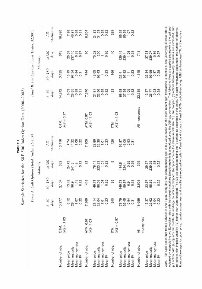
Table I presents the summary statistics of the options data. Here the aver-age price, moneyness, maturity, and IV for options in each moneyness–maturitysubgroup are reported for the daily 2–3 p.m. window data for the three-year

38

1990 1991 1992 1993 1994 1995 1996

annualized volatility

1997 1998 1999 2000 2001 2002

0.24

0.16

0.08

0.00

skewness

1990

0.6

0.4

0.2

�0.

0�

0.4

�0.

8

1991 1992 1993 1994 1995 1996 1997 1998 1999 2000 2001 2002

kurtosis

109

87

65

43

21

0

1990 1991 1992 1993 1994 1995 1996 1997 1998 1999 2000 2001 2002

FIGURE 1Annualized standard deviation, skewness, and kurtosis for daily S&P 500 index returns (1990–2002).

TA

BL

E I

Sam

ple

Sta

tist

ics

for

the

S&

P 5

00 I

ndex

Opt

ion

Dat

a (2

000–

2002

)

Pane

l A: C

all O

ptio

ns (

Tota

l Tra

des:

26,

154)

Pane

l B: P

ut O

ptio

ns (

Tota

l Tra

des:

32,

987)

Mat

urit

yM

atur

ity

6–60

60–1

80�

180

All

6–60

60–1

80�

180

All

days

days

days

Mat

urit

ies

days

days

days

Mat

urit

ies

Num

ber

of o

bs.

OT

M:

10,9

772,

107

332

13,4

16O

TM

:14

,842

3,43

561

318

,890

X/S

�1.

03X

/S�

0.97

Mea

n pr

ice

6.12

13.4

224

.73

7.74

6.03

13.1

525

.69

7.98

Mea

n m

atur

ity28

96.9

241.

344

.22

28.8

597

.54

237.

4548

.21

Mea

n m

oney

ness

1.07

1.13

1.2

1.08

0.89

0.84

0.83

0.88

Mea

n IV

0.22

0.22

0.22

0.22

0.31

0.3

0.27

0.31

Num

ber

of o

bs.

AT

M: 0

.97

7,36

941

822

7,80

9A

TM

: 0.9

77,

370

744

908,

204

X/S

�1.

03X

/S�

1.03

Mea

n pr

ice

21.1

449

.71

78.4

122

.89

21.9

148

.05

75.5

224

.93

Mea

n m

atur

ity22

.04

90.0

322

3.23

26.3

522

.56

92.4

325

031

.53

Mea

n m

oney

ness

1.01

1.01

1.01

1.01

0.99

11

0.99

Mea

n IV

0.23

0.25

0.22

0.23

0.22

0.23

0.26

0.22

Num

ber

of o

bs.

ITM

: 34

083

542

8IT

M:

423

166

4062

9X

/S�

0.97

X/S

�1.

03M

ean

pric

e78

.79

149.

7111

4.8

92.8

768

.68

123.

4112

9.49

86.9

9M

ean

mat

urity

26.4

599

.87

224.

443

.08

27.2

897

.82

239.

459

.39

Mea

n m

oney

ness

0.94

0.9

0.95

0.93

1.05

1.1

1.08

1.07

Mea

n IV

0.31

0.33

0.29

0.31

0.22

0.23

0.23

0.22

Num

ber

of o

bs.

All

18,6

862,

608

359

All

mon

eyne

ss22

,635

4,34

574

3m

oney

ness

Mea

n pr

ice

13.3

723

.57

29.2

712

.37

23.3

437

.31

Mea

n m

atur

ity25

.62

95.8

923

9.95

26.7

796

.68

239.

07M

ean

mon

eyne

ss1.

041.

11.

180.

930.

870.

86M

ean

IV0.

220.

220.

220.

280.

280.

27

Not

e.F

or e

ach

optio

n th

at t

rade

s be

twee

n 2

and

3 p.

m.

ever

y da

y, t

he c

orre

spon

ding

spo

t in

dex

valu

e ba

sed

on t

he m

ost

rece

nt s

pot

tran

sact

ion

is id

entifi

ed.

The

und

erly

ing

inte

rest

rat

e is

obta

ined

by

inte

rpol

atin

g tw

o E

urod

olla

r ra

tes

with

the

clo

sest

mat

uriti

es (

time-

to-m

atur

ity is

ann

ualiz

ed u

sing

the

365

-day

con

vent

ion)

. The

fol

low

ing

filte

rs a

re a

pplie

d se

para

tely

to

the

call

and

put

optio

n da

ta:

(a)

optio

ns t

hat

viol

ate

the

arbi

trag

e bo

unds

are

dro

pped

, (b

) op

tions

bel

ow t

he m

inim

um t

ick

size

of

are

drop

ped,

(c)

opt

ions

bel

ow s

ix-d

ay m

atur

ities

are

elim

inat

ed,

and

(d)

optio

ns w

ith im

plie

d vo

latil

ity (

IV)

high

er th

an 2

are

dro

pped

. The

IVs

are

calc

ulat

ed u

sing

the

IV s

urfa

ce a

s de

scrib

ed in

the

artic

le. F

or e

ach

mon

eyne

ss s

ubsa

mpl

e, th

e nu

mbe

r of

obs

erva

-tio

ns a

nd a

vera

ges

for

optio

n pr

ice,

mat

urity

, mon

eyne

ss, a

nd v

olat

ility

are

rep

orte

d fo

r ca

lls in

Pan

el A

and

for

puts

in P

anel

B. O

TM

, out

-of-

the-

mon

ey; A

TM

, at-

the-

mon

ey IT

M, i

n th

e m

oney

.

3 8



period, i.e., January 2000–December 2002. The summary statistics for sub-samples relate to short-term (6–60 days), medium-term (61–180 days), andlong-term (�180 days) maturities and correspond to three moneyness levels.OTM options are defined as those with moneyness (i.e., strike price/spot priceor X/S) above (below) 1.03 (0.97) for calls (puts). ATM options are defined asX/S lying between 0.97 and 1.03 and in-the-money or ITM options are thosewith X/S below (above) 0.97 (1.03) for calls (puts).

The moneyness and maturity-related biases are evident from Table I. Forexample, OTM put IVs dominate ITM put IVs and more so for shorter maturi-ties. Most of the option trading seems to be concentrated in short-term ATMand OTM calls and puts. Trades for OTM puts far exceed those of ATM puts,indicating that the former have been widely used as crash insurance. In general,trading is thin for ITM options and for maturities beyond two months. Hence,the subsequent analysis focuses on the ATM short-term options as they are veryliquid and have minimal pricing biases. The final sample consists of 7,369 calltrades and 7,370 put trades.

CONDITIONAL VOLATILITY AND SKEWNESSMODELS: ESTIMATION AND RESULTS

Model Estimation

Four time-series models are estimated in the following analysis. Model 1 is theGARCH(1, 1)-in-mean (GARCH-M) model with leverage and Monday effects(Harvey & Siddique, 1999) and is specified as

(1)

The leverage dummy dt�1 in the variance equation ht captures the asym-metric effect of negative shocks on volatility, whereas the weekly dummy Mont

captures the possibility of higher asymmetric information on Mondays (followingtwo non-trading days).

Model 2 is the EGARCH(1, 1)-M model, with the Monday effect, and isspecified as

(2)ln(ht) � b0 � b1 ln(ht�1) � b2a 0et�1 0 � B 2

pb � b3et�1 � b4Mont

rt � a0 � a1rt�1 � a2ht�1 � ut, ut � 2htet, (et 0�t�1) � N(0, 1)

dt�1 � e 0 if ut�1 � 0,1 if ut�1 � 0,

Mont � e1 if t � Monday0 otherwise.

ht � b0 � b1ht�1 � b2u2t�1 � b3dt�1u

2t�1 � b4Mont

rt � a0 � a1rt�1 � a2ht�1 � ut, ut � 2htet, (et 0�t�1) � N(0, 1)



where b3 captures the asymmetric volatility effect. Both models 1 and 2 permitunconditional skewness by modeling the leverage effect.

Model 3 is based on Hansen’s (1994) model and combines GARCH(1, 1)-Mwith leverage and Monday effects and time-varying conditional skewness anddegrees of freedom. The conditional skewness skt and degrees of freedom dft

are both expressed as functions of lagged residuals. The inverse of the degreesof freedom captures the kurtosis of the return distribution. Although a standardGARCH model provides only latent conditional volatility forecasts from thespot data, the GARCH model with conditional skewness provides both condi-tional volatility and skewness forecasts.2

Model 3 is specified as follows:

(3)

The density function for standardized residuals at time t implicit in model3 is the skewed t distribution defined as (time subscripts suppressed)

(3a)

where l is the skewness parameter constrained as �1 � l � 1, and h standsfor degrees of freedom bounded as 2 � h � .

The time t skewness parameter l in (3a) is a logistic function of skt in model3, i.e., , con-strained as �0.9 � lt � 0.9 (see Hansen, 1994, p. 723). Similarly, the degreesof freedom at time t or ht in the density function (3a) are expressed as a logisticfunction of dft in model 3, i.e.,

, bounded as 2.1 � ht � 30 (see Hansen, 1994, p. 719).Further, the constants a, b, and c are defined as follows:

(3b)a � 4lcah � 2h � 1

b, b2 � 1 � 3l2 � a2, c �((h � 1)�2)

2p(h � 2)(h�2).

(1 � e�(dft)) � 2.1ht � (30 � 2.1)�(1 � e�(dft) ) � 2.1 � 27.9�

lt � (0.9 � (�0.9))�(1� e�(skt)) � (�0.9) � 1.8�(1 � e�(skt)) � 0.9

g(z 0h, l) � µ b � c a1 �1

h � 2abz � a

1 � lb2b�(h�1)�2

, z � �ab

b � c a1 �1

h � 2abz � a

1 � lb2b�(h�1)�2

, z � �ab

dft � g0 � g1ut�1 � g2u2t�1.

skt � d0 � d1ut�1 � d2u2t�1

ht � b0 � b1ht�1 � b2u2t�1 � b3dt�1u

2t�1 � b4Mont

rt � a0 � a1rt�1 � a2ht�1 � ut, ut � 2htet, (et 0�t�1) � g(Z 0h, l)

2Volatility and skewness forecasts were also generated using Harvey and Siddique’s (1999) specification. Themodel estimation is sensitive to initial values. The optimization (based on Gauss optimum procedure) is highlyunstable and often does not converge. However, the Hansen (1994) model is found to be stable and easier tooperationalize for option trading purposes, where repeated out-of-sample estimation of volatility and skew-ness is required based on rolling samples.



This density function has a zero mean and unit variance. Setting l to zerogives us a regular t distribution and setting h to a high number over 30 and l tozero gives us a regular standard normal distribution. The inverse of the degreesof freedom captures the implicit fatness in the tails.

Model 4 is Hansen’s (1994) model with skewness and kurtosis restrictedto fixed non-zero intercepts and is specified as

(4)

Next a thorough statistical validation of the time-series models is presentedas a precursor to their use in option trading.

In-Sample Results

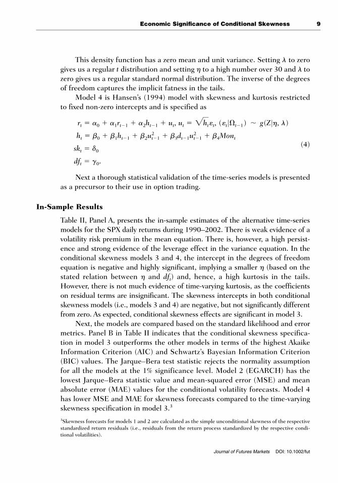
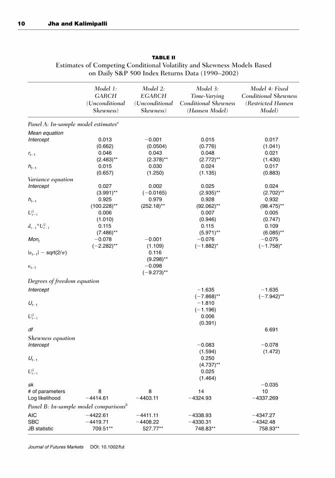
Table II, Panel A, presents the in-sample estimates of the alternative time-seriesmodels for the SPX daily returns during 1990–2002. There is weak evidence of avolatility risk premium in the mean equation. There is, however, a high persist-ence and strong evidence of the leverage effect in the variance equation. In theconditional skewness models 3 and 4, the intercept in the degrees of freedomequation is negative and highly significant, implying a smaller h (based on thestated relation between h and dft) and, hence, a high kurtosis in the tails.However, there is not much evidence of time-varying kurtosis, as the coefficientson residual terms are insignificant. The skewness intercepts in both conditionalskewness models (i.e., models 3 and 4) are negative, but not significantly differentfrom zero. As expected, conditional skewness effects are significant in model 3.

Next, the models are compared based on the standard likelihood and errormetrics. Panel B in Table II indicates that the conditional skewness specifica-tion in model 3 outperforms the other models in terms of the highest AkaikeInformation Criterion (AIC) and Schwartz’s Bayesian Information Criterion(BIC) values. The Jarque–Bera test statistic rejects the normality assumptionfor all the models at the 1% significance level. Model 2 (EGARCH) has thelowest Jarque–Bera statistic value and mean-squared error (MSE) and meanabsolute error (MAE) values for the conditional volatility forecasts. Model 4has lower MSE and MAE for skewness forecasts compared to the time-varyingskewness specification in model 3.3

dft � g0.

skt � d0

ht � b0 � b1ht�1 � b2u2t�1 � b3dt�1u

2t�1 � b4Mont

rt � a0 � a1rt�1 � a2ht�1 � ut, ut � 2htet, (et 0�t�1) � g(Z 0h, l)

3Skewness forecasts for models 1 and 2 are calculated as the simple unconditional skewness of the respectivestandardized return residuals (i.e., residuals from the return process standardized by the respective condi-tional volatilities).



TABLE II

Estimates of Competing Conditional Volatility and Skewness Models Based on Daily S&P 500 Index Returns Data (1990–2002)

Model 1: Model 2: Model 3: Model 4: Fixed GARCH EGARCH Time-Varying Conditional Skewness

(Unconditional (Unconditional Conditional Skewness (Restricted Hansen Skewness) Skewness) (Hansen Model) Model)

Panel A: In-sample model estimatesa

Mean equationIntercept 0.013 �0.001 0.015 0.017

(0.662) (0.0504) (0.776) (1.041)rt�1 0.046 0.043 0.048 0.021

(2.483)** (2.378)** (2.772)** (1.430)ht�1 0.015 0.030 0.024 0.017

(0.657) (1.250) (1.135) (0.883)Variance equationIntercept 0.027 0.002 0.025 0.024

(3.991)** (�0.0165) (2.935)** (2.702)**ht�1 0.925 0.979 0.928 0.932

(100.228)** (252.18)** (92.062)** (98.475)**0.006 0.007 0.005

(1.010) (0.946) (0.747)0.115 0.115 0.109

(7.486)** (5.971)** (6.085)**Mont �0.078 �0.001 �0.076 �0.075

(�2.282)** (1.109) (�1.882)* (�1.758)*|et�1| � sqrt(2/p) 0.116

(9.298)**et�1 �0.098

(�9.273)**

Degrees of freedom equation

Intercept �1.635 �1.635(�7.868)** (�7.942)**

Ut�1 �1.810(�1.196)

0.006(0.391)

df 6.691

Skewness equationIntercept �0.083 �0.078

(1.594) (1.472)Ut�1 0.250

(4.737)**0.025

(1.464)sk �0.035# of parameters 8 8 14 10Log likelihood �4414.61 �4403.11 �4324.93 �4337.269

Panel B: In-sample model comparisonsb

AIC �4422.61 �4411.11 �4338.93 �4347.27SBC �4419.71 �4408.22 �4330.31 �4342.48JB statistic 709.51** 527.77** 748.83** 758.93**

U2t�1

U2t�1

dt�1*U2t�1

U2t�1



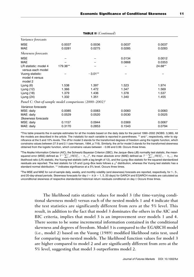
The likelihood ratio statistic values for model 3 (the time-varying condi-tional skewness model) versus each of the nested models 1 and 4 indicate thatthe test statistics are significantly different from zero at the 5% level. Thisresult, in addition to the fact that model 3 dominates the others in the AIC andBIC criteria, implies that model 3 is an improvement over models 1 and 4.There seems to be some incremental information contained in the conditionalskewness and degrees of freedom. Model 3 is compared to the EGARCH model(i.e., model 2) based on the Vuong (1989) modified likelihood ratio test, usedfor comparing non-nested models. The likelihood function values for model 3are higher compared to model 2 and are significantly different from zero at the5% level, suggesting that model 3 outperforms model 2.

TABLE II (Continued)

Variance forecasts

MSE 0.0037 0.0036 0.0037 0.0037MAE 0.0281 0.0275 0.0285 0.0283

Skewness forecasts

MSE – – 0.0134 0.0012MAE – – 0.0868 0.0353LR statistic: model 4 179.36** – – 24.68**versus each model

Vuong statistic: – �3.01** – –model 4 versus model 2

Ljung (6) 1.538 1.397 1.523 1.974Ljung (12) 1.366 1.472 1.347 1.569Ljung (18) 1.379 1.436 1.378 1.537Ljung (24) 1.332 1.351 1.340 1.455

Panel C: Out-of-sample model comparisons (2000–2002)c

Variance forecastsMSE: daily 0.0085 0.0083 0.0083 0.0083MAE: daily 0.0529 0.0520 0.0530 0.0525Skewness forecastsMSE: daily 0.1157 0.0944 0.0369 0.0067MAE: daily 0.3170 0.2853 0.1543 0.0794

aThis table presents the in-sample estimates for all the models based on the daily data for the period 1990–2002 (NOBS: 3,389). Allthe models are described in the article. The t-statistic for each variable is reported in parentheses. ** and *, respectively, refer to sig-nificance at the 5 and 10% levels. The df for model 3 stands for the transformed degrees of freedom using the logistic function, whichconstrains values between 27.9 and 2.1 (see Hansen, 1994, p 719). Similarly, the sk for model 3 stands for the transformed skewnessobtained from the logistic function, which constrains values between �0.99 and 0.99. Occurs three times.

bThe Akaike Information Criterion (AIC), the Schwartz Bayesian Criterion (SBC), the Jarque–Bera (JB) normality test statistic, the mean-squared error (MSE) defined as , the mean absolute error (MAE) defined as thelikelihood ratio (LR) statistic, the Vuong test statistic (with a lag length of 12), and the Ljung–Box statistic for the squared standardizedresiduals are reported. The test statistic for LR and Ljung–Box tests follows a x2 distribution, whereas the Vuong test statistic has astandard normal distribution. ** indicates significance at a 5% level. Occurs three times.

cThe MSE and MAE for out-of-sample daily, weekly, and monthly volatility (and skewness) forecasts are reported, respectively, for 1-, 5-,and 20-day-ahead periods. Skewness forecasts for day t � k (k � 1, 5, 20 days) for GARCH and EGARCH models are calculated asunconditional skewness of respective standardized historical return residuals conditional on day t. Occurs three times.

T �1a

Tt�1 0RES 2

t�1 � ht�1 0 ,T�1a

Tt�1[RES 2

t�1 � ht�1]2



The Ljung–Box statistic for squared standardized residuals is insignificantfor all models, indicating that residual autocorrelation is insignificant. In sum-mary, the results show that model 3, the time-varying conditional skewnessmodel, performs better than the other three models based on the AIC, BIC,and Ljung–Box metrics.

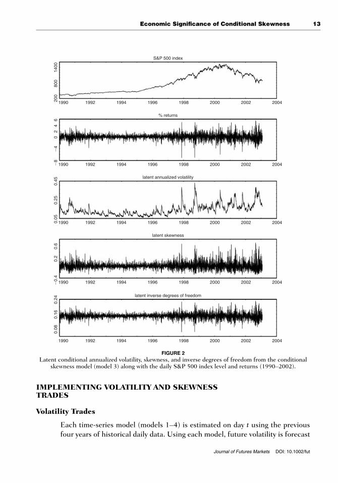
Figure 2 presents the in-sample annualized volatility, skewness, andinverse degrees of freedom forecasts from the conditional skewness model(corresponding to ht, skt, and inverse of dft variables in model 3) for the period1990–2002; the level and returns for the daily SPX data are also plotted. The1991 Gulf War, the 1997–1998 Asian crisis, the 1998–1999 Russian crisis, andthe 2001 burst of the technology bubble are periods of high return shocks and also of high volatility and skewness. Negative skewness becomes morepronounced, i.e., underlying markets become more bearish in these periodsconsistent with the unconditional plots in Figure 1. These are also periods whenreturn distributions become fat tailed (periods of low degrees of freedom corre-spond to high tail fatness and vice versa).

Out-of-Sample Results

Given that there could be concerns of over-fitting in-sample with the condi-tional skewness specification, an out-of-sample analysis is performed. Theanalysis is also extended to weekly and monthly horizons. The three-year peri-od, i.e., 2000–2002 (corresponding to the option data sample) is the out-of-sample period. Forecasts are generated using four-year rolling windows.

Panel C of Table II presents the MSE and MAE values for daily horizonsfor out-of-sample variance and skewness forecasts. All the models provide sim-ilar volatility forecasts. At all horizons, the MSE values for variance forecastsare similar across models. The EGARCH model performs marginally betterbased on the MAE criterion. For out-of-sample skewness forecasts at the dailyhorizon, model 4, the fixed skewness model, seems to be associated with lowerMSE and MAE metrics compared to model 3, consistent with the findings in-sample. However, in unreported results, model 3 dominates model 4 based onthe MAE criterion at the weekly and monthly horizons.

In summary, Table II results suggest mixed evidence in favor of model 3.The conditional volatility dynamics in model 3 seem to be unaffected by thetime-varying third moments. The differences in the diagnostic metrics forvolatility forecasts across the models are much smaller compared to skewnessforecasts at all three horizons.

Next the out-of-sample performance of the models based on option trad-ing is evaluated.



IMPLEMENTING VOLATILITY AND SKEWNESSTRADES

Volatility Trades

Each time-series model (models 1–4) is estimated on day t using the previousfour years of historical daily data. Using each model, future volatility is forecast

200

1990 1992 1994 1996

S&P 500 index

1998 2000 2002 2004

800

1400

% returns

1990 1992 1994 1996 1998 2000 2002 2004

�4

�8

42

06

latent annualized volatility

1990 1992 1994 1996 1998 2000 2002 20040.05

0.25

0.45

latent skewness

1990 1992 1994 1996 1998 2000 2002 2004�0.

40.

20.

6

latent inverse degrees of freedom

1990 1992 1994 1996 1998 2000 2002 2004

0.16

0.08

0.24

FIGURE 2Latent conditional annualized volatility, skewness, and inverse degrees of freedom from the conditional

skewness model (model 3) along with the daily S&P 500 index level and returns (1990–2002).



each day until the maturity of the straddle, and the arithmetic average of suchfuture volatility forecasts is obtained. This measure serves as a volatility proxyto price an option on day t using the Black–Scholes pricing formula.

The following analysis investigates whether the volatility forecasts from eachgiven conditional volatility model can be used to formulate profitable out-of-sample straddle trading strategies in the options market. A long (short) straddlerepresents a long (short) position in one call and one put option on an underlyingwith identical strike price and maturity.4 Straddle positions help traders exploitsignificant differences between their private and market estimates of spot volatil-ity. The method used is a modified version of the approach used by Noh, Engle,and Kane (1994), who show that simple GARCH models outperform IV modelsfor investors trading in ATM straddles, after accounting for transaction costs.Bakshi et al. (1997) find that for ATM options, the Black–Scholes model does aswell as SV-based pricing models. Hence, as the first step, the Black–Scholesmodel (adjusted for dividends) is used to price the SPX options, which areEuropean in nature and have no early exercise possibilities or wild-card options.

Out-of-sample volatility forecasts are used to trade in short-term (i.e.,maturity 6–60 days) ATM delta-neutral straddles. First, using the out-of-sampledaily volatility forecast for day t, the delta-neutral straddle is obtained for thatday. In particular, given that delta of the call and put is, respectively, N(d1) andN(d1) � 1, the strike price x that gives a delta-neutral straddle on day t can besolved as

(5)

where S, rf, s, and (T � t)/365 refer to the spot price, risk-free rate, volatility,and annualized option maturity, respectively. Next, the traded straddle combi-nation on day t using ATM calls and puts on that day with strike price closest tothe x described in Equation (5) is obtained. Finally the price of the ATM delta-neutral straddle is obtained using the Black–Scholes model.

ATM delta-neutral straddles are bought (sold) on day t depending onwhether the straddle is under (or over) priced relative to the closing marketstraddle price on that day. When the straddle is purchased (sold), it is assumedthat funds can be borrowed (invested) funds at the risk-free rate. The rate ofreturn is calculated as follows:

(6a)

(6b)Return on selling a straddle�(Ct�1 � Pt�1 � Ct � Pt)

Ct � Pt� rf

Return on buying a straddle �Ct�1 � Pt�1 � Ct � Pt

Ct � Pt� rf

N(d1) � N(d1) � 1 � 0, x �S

e(�rf�s2�2)(T�t)�365

4Other straddle variants with different strike and maturity horizons may be used, but are not considered inthis study.



where Ct and Pt refer to the call and put prices of SPX options. This tradingprocess is repeated for each trading day in the sample.

For all trades, the bid–ask spread filter is applied.5 The trade occurs onlywhen the absolute price difference between the model and the market price isexpected to exceed half of the straddle bid–ask spread of 5.70% (where 5.70%is obtained as the average of the bid–ask spread of 5.5% for calls and 5.9% forputs; see Santa-Clara & Saretto, 2005, Table 9).6 The bid–ask spread of 5.70%plus commission cost of 0.5% toward the transaction costs is applied. The 0.5%commission cost corresponds to a trader with a $48,000 investment who pays a commission amounting to $120 plus 0.25% of the dollar amount based on astandard commission schedule (see Hull, 2000, p. 160). The profits net oftransaction costs and bid–ask filters are compared across the models.

Skewness Trades

Next, out-of-sample skewness forecasts are used to trade in ATM delta-neutralstrips and straps in addition to the straddles.7 Although a straddle consists of along position in a call and a put with the same strike price and maturity, a strip(strap) consists of a long position in one call and two puts (two calls and oneput) with the same strike price and expiration. Although straddles provide sym-metric payoffs in bull and bear markets, strips and straps have asymmetric pay-offs, with higher payoffs compared to straddles in down and up markets,respectively. Therefore, if skewness is predictable, an option trader might pre-fer to take positions in strips or straps depending on the expected payoffs.

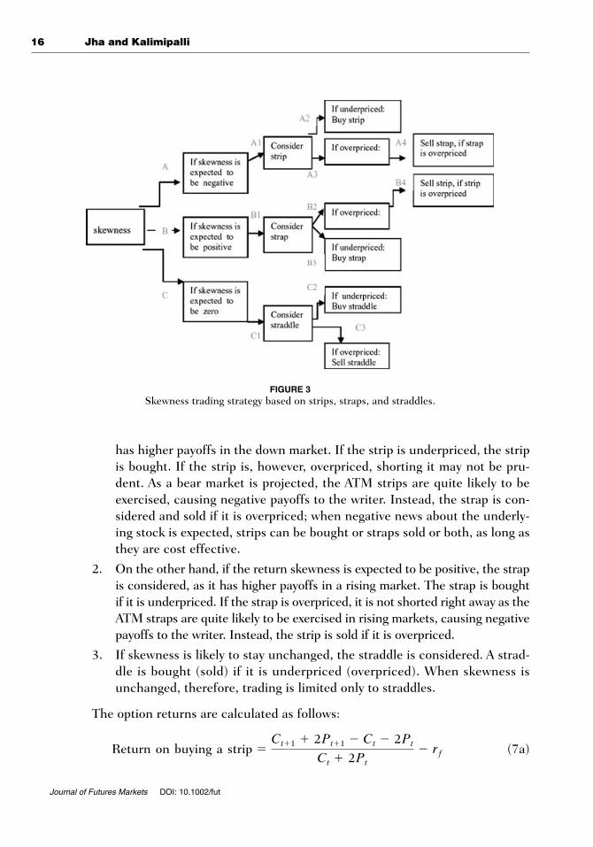
Broadly, three outcomes are expected, depending on whether skewness isexpected to be positive, negative, or zero as shown in Figure 3.

Similar to volatility trades, the average volatility forecast for each model at timet for the remaining maturity period of an option is obtained. Although skewnessforecasts for models 3 and 4 are obtained from the respective model dynamics,those for the GARCH and EGARCH models are calculated as a simple uncondi-tional skewness of respective standardized historical returns. Using the out-of-sample daily volatility forecasts, delta-neutral strip, strap, and straddle are obtainedfor each trading day, and their Black–Scholes model prices are calculated.

Strips, straps, and straddles are bought (sold) following the trading strate-gy depicted in Figure 3 and outlined below:

1. If the return skewness is expected to be negative, it implies negative expec-tations regarding the market. In this scenario the strip is considered, as it

5Similar bid–ask spreads are used by Chan, Jha, and Kalimipalli (2009).6A fixed bid–ask filter is assumed as access to intra-day quote data is not available.7Ait-Sahalia et al. (2001), Bollen and Whaley (2004), and Santa-Clara and Saretto (2005) also provide a dis-cussion of option-based trading.



has higher payoffs in the down market. If the strip is underpriced, the stripis bought. If the strip is, however, overpriced, shorting it may not be pru-dent. As a bear market is projected, the ATM strips are quite likely to beexercised, causing negative payoffs to the writer. Instead, the strap is con-sidered and sold if it is overpriced; when negative news about the underly-ing stock is expected, strips can be bought or straps sold or both, as long asthey are cost effective.

2. On the other hand, if the return skewness is expected to be positive, the strapis considered, as it has higher payoffs in a rising market. The strap is boughtif it is underpriced. If the strap is overpriced, it is not shorted right away as theATM straps are quite likely to be exercised in rising markets, causing negativepayoffs to the writer. Instead, the strip is sold if it is overpriced.

3. If skewness is likely to stay unchanged, the straddle is considered. A strad-dle is bought (sold) if it is underpriced (overpriced). When skewness isunchanged, therefore, trading is limited only to straddles.

The option returns are calculated as follows:

(7a)Return on buying a strip �Ct�1 � 2Pt�1 � Ct � 2Pt

Ct � 2Pt� rf

FIGURE 3Skewness trading strategy based on strips, straps, and straddles.



(7b)

(7c)

(7d)

As in the case of straddle trades, in the long position, the agent borrows atthe risk-free rate, whereas in the short position, she invests the proceeds in arisk-free asset. The process is repeated for each trading day in the sample.Transaction cost filters are applied as described for volatility trades. Thebid–ask filters for straps and strips are set at 5.63 and 5.77%, respectively(based on bid–ask spread of 5.5% for calls and 5.9% for puts; see Santa-Clara& Saretto, 2005, Table 9).

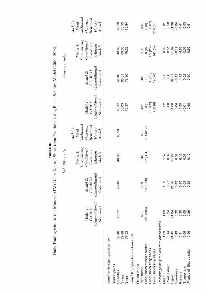
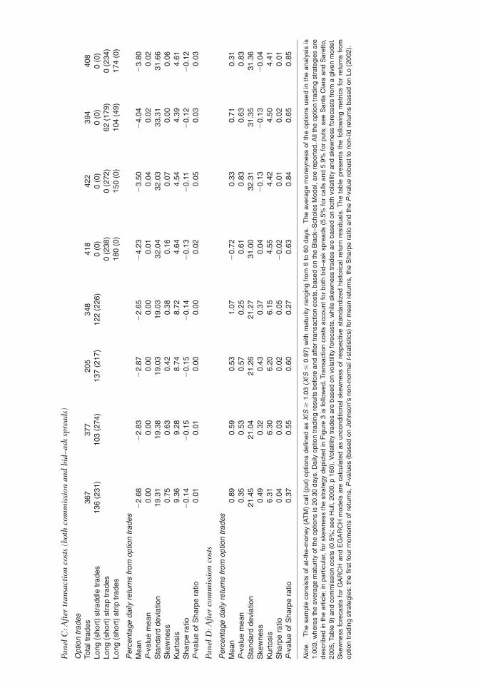
Results From Option Trading

Table III presents the results from option trading using the Black–Scholesmodel. Volatility trades refer to trading in straddles, whereas skewness tradesrefer to trading in straddles, strips, and straps. Panel A reports the average mar-ket and model prices across all four specifications. The model prices indicatethat straddles, strips, and straps are all overpriced in the market, with the over-pricing being the least for the time-varying conditional skewness model. Theoverpricing seems to arise mainly from the ATM calls (results not reported).The average moneyness of straddles used in the sample is almost one, whereasthe average maturity is about 20 days.

Panels B and C, respectively, in Table III report trading results before andafter transaction costs and bid–ask filters. Straddles are sold more often thanbought for all the models, with EGARCH accounting for the maximum shortpositions. When skewness is accounted for, straddles are not traded. As skew-ness forecasts are predominantly negative for all models except for the condi-tional skewness model, trading is diverted to strips, i.e., node A1 in Figure 3.Depending on whether the strips are underpriced (or overpriced) in the market,trades are diverted to node A2-long strip positions (or A4-short strap positions).Trades at node A4 outnumber trades at node A3, implying that the strips aregenerally overpriced. In the case of model 3, there is also some trading instraps, i.e., node B3.

Daily trading returns both before and after transaction costs are examinednext. For option returns, the p-values are reported and correspond to the

Return on selling a strap � � a2Ct�1 � Pt�1 � 2Ct � Pt2Ct � Pt

b � rf.

Return on buying a strap �2Ct�1 � Pt�1 � 2Ct � Pt

2Ct � Pt� rf

Return on selling a strip � �aCt�1 � 2Pt�1 � Ct � 2PtCt � 2Pt

b � rf

TA

BL

E I

II

Dai

ly T

radi

ng w

ith

At-

the-

Mon

ey (

AT

M)

Del

ta-N

eutr

al S

hort

-ter

m P

osit

ions

Usi

ng B

lack

–Sch

oles

Mod

el (

2000

–200

2)

Vola

tili

ty T

rade

sS

kew

ness

Tra

des

Mod

el 4

:M

odel

4:

Mod

el 3

:Fi

xed

Mod

el 3

:Fi

xed

Tim

e-Va

ryin

gC

ondi

tion

alT

ime-

Vary

ing

Con

diti

onal

Mod

el 1

:M

odel

2:

Con

diti

onal

S

kew

ness

Mod

el 1

:M

odel

2:

Con

diti

onal

S

kew

ness

GA

RC

H

EG

AR

CH

Ske

wne

ss(R

estr

icte

dG

AR

CH

E

GA

RC

HS

kew

ness

(Res

tric

ted

(Unc

ondi

tion

al

(Unc

ondi

tion

al

(Han

sen

Han

sen

(Unc

ondi

tion

al

(Unc

ondi

tion

al

(Han

sen

Han

sen

Ske

wne

ss)

Ske

wne

ss)

Mod

el)

Mod

el)

Ske

wne

ss)

Ske

wne

ss)

Mod

el)

Mod

el)

Pane

l A: A

vera

ge o

ptio

n pr

ices

Mar

ket p

rices

Str

addl

es50

.46

48.1

746

.48

48.8

348

.50

48.1

746

.48

48.8

348

.50

Str

aps

72.8

868

.03

65.6

169

.03

68.5

5S

trip

s77

.52

75.3

772

.90

76.3

575

.84

Pane

l B: B

efor

e tr

ansa

ctio

n co

sts

Opt

ion

trad

esTo

tal t

rade

s51

851

851

851

849

249

148

048

5Lo

ng (

shor

t) s

trad

dle

trad

es21

2 (3

06)

180

(338

)21

7 (3

01)

201

(317

)0

(0)

0 (0

)0

(0)

0 (0

)Lo

ng (

shor

t) s

trap

trad

es0

(262

)0

(295

)85

(20

2)0

(267

)Lo

ng (

shor

t) s

trip

trad

es23

0 (0

)19

6 (0

)14

1 (5

2)21

8 (0

)

Per

cent

age

daily

ret

urns

from

opt

ion

trad

esM

ean

1.39

1.09

1.03

1.57

�0.

220.

830.

990.

81P

-val

ue m

ean

0.14

0.24

0.27

0.09

0.88

0.58

0.51

0.58

Sig

ma

21.4

521

.04

21.2

621

.27

31.0

032

.31

31.6

731

.36

Ske

wne

ss0.

490.

320.

430.

370.

04�

0.13

�0.

17�

0.04

Kur

tosi

s6.

316.

306.

206.

154.

554.

424.

534.

41S

harp

e ra

tio0.

060.

050.

050.

07�

0.01

0.02

0.03

0.03

P-v

alue

of

Sha

rpe

ratio

0.16

0.26

0.29

0.10

0.88

0.60

0.53

0.61

Pane

l C: A

fter

tra

nsac

tion

cos

ts (

both

com

mis

sion

and

bid

–ask

spr

eads

)

Opt

ion

trad

esTo

tal t

rade

s36

737

720

534

841

842

239

440

8Lo

ng (

shor

t) s

trad

dle

trad

es13

6 (2

31)

103

(274

)13

7 (2

17)

122

(226

)0

(0)

0 (0

)0

(0)

0 (0

)Lo

ng (

shor

t) s

trap

trad

es0

(238

)0

(272

)62

(17

9)0

(234

)Lo

ng (

shor

t) s

trip

trad

es18

0 (0

)15

0 (0

)10

4 (4

9)17

4 (0

)

Per

cent

age

daily

ret

urns

from

opt

ion

trad

esM

ean

�2.

68�

2.83

�2.

87�

2.65

�4.

23�

3.50

�4.

04�

3.80

P-v

alue

mea

n0.

000.

000.

000.

000.

010.

040.

020.

02S

tand

ard

devi

atio

n19

.31

19.3

819

.03

19.0

332

.04

32.0

333

.31

31.6

6S

kew

ness

0.75

0.63

0.42

0.38

0.16

0.07

0.00

0.06

Kur

tosi

s9.

369.

288.

748.

724.

644.

544.

394.

61S

harp

e ra

tio�

0.14

�0.

15�

0.15

�0.

14�

0.13

�0.

11�

0.12

�0.

12P

-val

ue o

f Sha

rpe

ratio

0.01

0.01

0.00

0.00

0.02

0.05

0.03

0.03

Pane

l D: A

fter

com

mis

sion

cos

ts

Per

cent

age

daily

ret

urns

from

opt

ion

trad

esM

ean

0.89

0.59

0.53

1.07

�0.

720.

330.

710.

31P

-val

ue m

ean

0.35

0.53

0.57

0.25

0.61

0.83

0.63

0.83

Sta

ndar

d de

viat

ion

21.4

521

.04

21.2

621

.27

31.0

032

.31

31.3

531

.36

Ske

wne

ss0.

490.

320.

430.

370.

04�

0.13

�0.

13�

0.04

Kur

tosi

s6.

316.

306.

206.

154.

554.

424.

504.

41S

harp

e ra

tio0.

040.

030.

020.

05�

0.02

0.01

0.02

0.01

P-v

alue

of S

harp

e ra

tio0.

370.

550.

600.

270.

630.

840.

650.

85

Not

e.T

he s

ampl

e co

nsis

ts o

f at

-the

-mon

ey (

AT

M)

call

(put

) op

tions

defi

ned

as X

/S�

1.03

(X

/S�

0.97

) w

ith m

atur

ity r

angi

ng f

rom

6 t

o 60

day

s.

The

ave

rage

mon

eyne

ss o

f th

e op

tions

use

d in

the

ana

lysi

s is

1.00

3, w

hera

s th

e av

erag

e m

atur

ity o

f the

opt

ions

is 2

0.30

day

s. D

aily

opt

ion

trad

ing

resu

lts b

efor

e an

d af

ter

tran

sact

ion

cost

s, b

ased

on

the

Bla

ck–S

chol

es M

odel

, are

rep

orte

d. A

ll th

e op

tion

trad

ing

stra

tegi

es a

rede

scrib

ed in

the

artic

le; i

n pa

rtic

ular

, for

ske

wne

ss th

e st

rate

gy d

epic

ted

in F

igur

e 3

is fo

llow

ed. T

rans

actio

n co

sts

acco

unt f

or b

oth

bid–

ask

spre

ads

(5.5

% fo

r ca

lls a

nd 5

.9%

for

puts

; see

San

ta C

lara

and

Sar

etto

,20

05, T

able

9)

and

com

mis

sion

cos

ts (

0.5%

; see

Hul

l, 20

00, p

160

). V

olat

ility

trad

es a

re b

ased

on

vola

tility

fore

cast

s, w

hile

ske

wne

ss tr

ades

are

bas

ed o

n bo

th v

olat

ility

and

ske

wne

ss fo

reca

sts

from

a g

iven

mod

el.

Ske

wne

ss f

orec

asts

for

GA

RC

H a

nd E

GA

RC

H m

odel

s ar

e ca

lcul

ated

as

unco

nditi

onal

ske

wne

ss o

f re

spec

tive

stan

dard

ized

his

toric

al r

etur

n re

sidu

als.

The

tab

le p

rese

nts

the

follo

win

g m

etric

s fo

r re

turn

s fr

omop

tion

trad

ing

stra

tegi

es: t

he fi

rst f

our

mom

ents

of r

etur

ns, P

-val

ues

(bas

ed o

n Jo

hnso

n’s

non-

norm

al t-

stat

istic

s) fo

r m

ean

retu

rns,

the

Sha

rpe

ratio

and

the

P-v

alue

rob

ust t

o no

n-iid

ret

urns

bas

ed o

n Lo

(20

02).



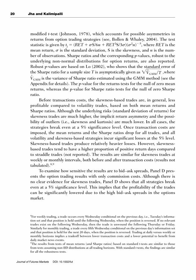
modified t-test (Johnson, 1978), which accounts for possible asymmetries inreturns from option trading strategies (see, Bollen & Whaley, 2004). The teststatistic is given by tj � (RET � sS/6n � RET2S/3s)(s2n)�.5, where RET is themean return, s is the standard deviation, S is the skewness, and n is the num-ber of observations. Sharpe ratios and the corresponding p-values, robust to theunderlying non-normal distributions for option returns, are also reported.Robust p-values are based on Lo (2002), who shows that the standard error ofthe Sharpe ratio for a sample size T is asymptotically given as ,where

is the variance of Sharpe ratio estimated using the GMM method (see theAppendix for details). The p-value for the returns tests for the null of zero meanreturns, whereas the p-value for Sharpe ratio tests for the null of zero Sharperatio.

Before transactions costs, the skewness-based trades are, in general, lessprofitable compared to volatility trades, based on both mean returns andSharpe ratios. Although the underlying risks (standard deviation of returns) forskewness trades are much higher, the implicit return asymmetry and the possi-bility of outliers (i.e., skewness and kurtosis) are much lower. In all cases, thestrategies break even at a 5% significance level. Once transaction costs areimposed, the mean returns and the Sharpe ratios drop for all trades, and allvolatility and skewness-based strategies incur significant losses at the 5% level.Skewness-based trades produce relatively heavier losses. However, skewness-based trades tend to have a higher proportion of positive return days comparedto straddle trades (not reported). The results are similar for skewness trades atweekly or monthly intervals, both before and after transaction costs (results nottabulated).8,9

To examine how sensitive the results are to bid–ask spreads, Panel D pres-ents the option trading results with only commission costs. Although there isno clear evidence for skewness trades, Panel D shows that all strategies breakeven at a 5% significance level. This implies that the profitability of the tradescan be significantly lowered due to the high bid–ask spreads in the optionsmarket.

VGMM

2VGMM�T

8For weekly trading, a trade occurs every Wednesday conditional on the previous day, i.e., Tuesday’s informa-tion set and that position is held until the following Wednesday, when the position is reversed. If no relevanttrades exist on the following Wednesday, then the trade is unwound the following Thursday or Friday.Similarly for monthly trading, a trade every fifth Wednesday conditional on the previous day’s information setand that position is held for the next 20 days, when the position is reversed. Trading at daily versus weekly ormonthly horizons implies a tradeoff between lower transaction costs and a lower potential to benefit fromdaily market news events.9The results from tests of mean returns (and Sharpe ratios) based on standard t-tests are similar to thosefrom tests assuming non-IID distributions at all trading horizons. With standard t-tests, the findings are similarfor all the robustness tests.



ROBUSTNESS TESTS

Alternative Pricing Models

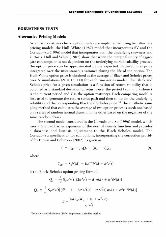
As a first robustness check, option trades are implemented using two alternatepricing models: the Hull–White (1987) model that incorporates SV and theCorrado–Su (1996) model that incorporates both the underlying skewness andkurtosis. Hull and White (1987) show that when the marginal utility of aggre-gate consumption is not dependent on the underlying market volatility process,the option price can be approximated by the expected Black–Scholes priceintegrated over the instantaneous variance during the life of the option. TheHull–White option price is obtained as the average of Black and Scholes pricesover N simulations (N � 15,000) for each time-series model. The Black andScholes price for a given simulation is a function of return volatility that isobtained as a standard deviation of returns over the period t to t � T (where tis the current period and T is the option maturity). Each competing model isfirst used to generate the return series path and then to obtain the underlyingvolatility and the corresponding Black and Scholes price.10 The antithetic sam-pling method that calculates the average of two option prices is used: one basedon a series of random normal draws and the other based on the negatives of thesame random draws.

The second model considered is the Corrado and Su (1996) model, whichuses a Gram–Charlier expansion of the normal density function and provides a skewness and kurtosis adjustment to the Black–Scholes model. TheCorrado–Su specification for call options, incorporating the correction provid-ed by Brown and Robinson (2002), is given as

(8)

where

is the Black–Scholes option-pricing formula.

d �ln(S0�K) � (r � s2�2)t

s2t

Q4 �14¡

S0s2t[(d2 � 1 � 3s2t(d � s2t)) n(d) � s3t3�2N(d)]

Q3 �13!

S0s2t[(2s2t � d)n(d) � s2tN(d)]

CBS � S0N(d) � Ke�rtN(d � s2t)

C � CBS � m3Q3 � (m4 � 3)Q4

10Bollerslev and Mikkelsen (1996) implement a similar method.



and

Corrado and Su (1996, 1997) show that a generalized option-pricing modelthat incorporates both skewness and kurtosis corrects existing pricing biases inthe Black–Scholes model, especially for deep OTM or deep ITM options.11

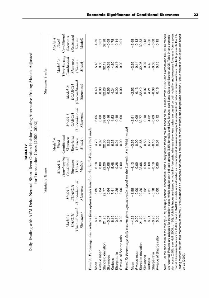
Table IV Panel A indicates that the posttransaction cost returns andSharpe ratios for all strategies are lower when the Hull–White model is used,compared to the Black–Scholes option-pricing results shown in Panel C, Table III.The results indicate a significant negative exposure across all trades and time-series models, with losses from volatility trades being substantially higher com-pared to the skewness-based trades.

Panel B presents the results from the Corrado–Su model. The skewness-based trades now all break even; the p-values indicate that the transaction costadjusted mean returns and Sharpe ratios are not statistically significantly dif-ferent from zero. The skewness-based trades clearly outperform the straddletrades, which are associated with significant losses. Untabulated results indi-cate that that the Corrado–Su model generates significant profits before trans-action costs at weekly and monthly horizons, with skewness trades dominatingthe volatility-based trades. This implies that using a generalized option-pricingmodel can help minimize losses, especially for trades in strips and straps.Although there are significant losses from trades while using the Black–Scholesand Hull–White models, the Corrado–Su model produces the least loss expo-sure particularly for the skewness-based trades. Though the trading perform-ance can be enhanced by the Corrado–Su model, the net option profits stilldepend upon the underlying bid–ask spreads.

Trading with Option Implied Volatility (IV)

Finally, the trading performance using option IV forecasts as the volatility proxyis examined. Option IVs extracted from cross-sectional option data are forward-looking in nature and have both moneyness and maturity dimensions. The IV isobtained based on a volatility surface using the IV function approach (seeChristoffersen, 2003, p. 138; Christoffersen & Jacobs, 2004). The volatility sur-face is defined in log form as a polynomial function of maturity and moneyness,and its parameters are obtained by minimizing the difference between the mar-ket and Black–Scholes model prices, observed during the 2–3 p.m. time windowevery trading day. Dumas et al. (1998) show that this approach outperforms

n(d) �1

22p exp(�d2�2).

11This study uses the SNP approach applied by Corrado and Su (1996, 1997) for the sensitivity analysis. Thetesting of the GST approach proposed by Lim et al. (2005, 2006) will be used in future work.


TA

BL

E I

V

Dai

ly T

radi

ng w

ith

AT

M D

elta

-Neu

tral

Sho

rt-T

erm

Opt

ion

Posi

tion

s U

sing

Alt

erna

tive

Pri

cing

Mod

els-

Adj

uste

d fo

r Tr

ansa

ctio

n C

osts

(20

00–2

002)

Vola

tili

ty T

rade

sS

kew

ness

Tra

des

Mod

el 4

:M

odel

4:

Mod

el 3

:Fi

xed

Mod

el 3

:Fi

xed

Tim

e-Va

ryin

gC

ondi

tion

alT

ime-

Vary

ing

Con

diti

onal

Mod

el 1

:M

odel

2:

Con

diti

onal

S

kew

ness

Mod

el 1

:M

odel

2:

Con

diti

onal

S

kew

ness

GA

RC

H

EG

AR

CH

Ske

wne

ss(R

estr

icte

dG

AR

CH

E

GA

RC

HS

kew

ness

(Res

tric

ted

(Unc

ondi

tion

al

(Unc

ondi

tion

al

(Han

sen

Han

sen

(Unc

ondi

tion

al

(Unc

ondi

tion

al

(Han

sen

Han

sen

Ske

wne

ss)

Ske

wne

ss)

Mod

el)

Mod

el)

Ske

wne

ss)

Ske

wne

ss)

Mod

el)

Mod

el)

Pane

l A: P

erce

ntag

e d

aily

ret

urns

from

opt

ion

trad

es b

ased

on

the

Hul

l–W

hite

(19

87)

mod

el

Mea

n�

6.40

�5.

85�

6.18

�4.

70�

6.05

�6.

40�

5.48

�4.

55P

-val

ue m

ean

0.01

0.04

0.00

0.02

0.00

0.00

0.00

0.01

Sta

ndar

d de

viat

ion

21.2

522

.77

22.2

022

.30

32.0

832

.28

32.1

932

.98

Ske

wne

ss�

0.07

0.64

�0.

080.

26�

0.16

0.55

�0.

33�

0.09

Kur

tosi

s6.

197.

415.

486.

354.

534.

344.

604.

78S

harp

e ra

tio�

0.30

�0.

26�

0.28

�0.

21�

0.19

�0.

20�

0.17

�0.

14P

-val

ue o

f Sha

rpe

ratio

0.00

0.00

0.00

0.00

0.00

0.00

0.00

0.01

Pane

l B: P

erce

ntag

e da

ily

retu

rns

from

opt

ion

trad

es b

ased

on

the

Cor

rado

–Su

(199

6) m

odel

Mea

n�

4.22

�3.

98�

4.13

�3.

55�

2.91

�2.

52�

2.65

�2.

68P

-val

ue m

ean

0.00

0.00

0.00

0.00

0.09

0.13

0.14

0.13

Sta

ndar

d de

viat

ion

21.7

022

.20

22.0

621

.86

32.7

732

.42

32.9

532

.33

Ske

wne

ss0.

600.

520.

580.

530.

180.

070.

070.

13K

urto

sis

6.91

7.31

6.68

6.72

4.32

4.21

4.43

4.36

Sha

rpe

ratio

�0.

20�

0.18

�0.

19�

0.16

�0.

09�

0.08

�0.

08�

0.08

P-v

alue

of S

harp

e ra

tio0.

000.

000.

000.

010.

120.

160.

150.

15

Not

e.F

or th

e sh

ort t

erm

at-

the-

mon

ey (

AT

M)

call

(put

) op

tions

, des

crib

ed in

Tab

le I,

dai

ly o

ptio

n tr

adin

g re

sults

bas

ed o

n th

e H

ull a

nd W

hite

(19

87)

and

Cor

rado

and

Su

(199

6) m

odel

sar

e re

port

ed. R

etur

ns a

re a

djus

ted

for

tran

sact

ion

cost

s, w

hich

incl

ude

both

bid

–ask

spr

eads

(5.

5% fo

r ca

lls a

nd 5

.9%

for

puts

; see

San

ta C

lara

and

Sar

etto

, 200

5, T

able

9)

and

com

mis

-si

on c

osts

(0.

5%;

see

Hul

l, 20

00,

p 16

0).

Vol

atili

ty t

rade

s ar

e ba

sed

on v

olat

ility

for

ecas

ts,

whe

reas

ske

wne

ss t

rade

s ar

e ba

sed

on b

oth

vola

tility

and

ske

wne

ss f

orec

asts

fro

m a

giv

enm

odel

. Ske

wne

ss fo

reca

sts

for

GA

RC

H a

nd E

GA

RC

H m

odel

s ar

e ca

lcul

ated

as

unco

nditi

onal

ske

wne

ss o

f res

pect

ive

stan

dard

ized

his

toric

al r

etur

n re

sidu

als.

The

tabl

e pr

esen

ts th

e fo

l-lo

win

g m

etric

s: th

e fir

st fo

ur m

omen

ts o

f ret

urns

, P-v

alue

s (b

ased

on

John

son’

s no

n-no

rmal

t-st

atis

tics)

for

mea

n re

turn

s, th

e S

harp

e ra

tio a

nd th

e P

-val

ue r

obus

t to

non-

iid r

etur

ns b

ased

on L

o (2

002)

.



many of the deterministic volatility models. Christoffersen (2003) shows thatthe IV function approach can be used as a robust benchmark for forecastingpurposes. Obtaining IVs by minimizing market and model price errors, throughthe IV function approach, helps address the smile biases and measurementerrors.

The model prices are obtained using the Black–Scholes model. The IVforecast for each delta-neutral ATM straddle is computed on a given day as anaverage of the underlying call and put IVs, where the IV forecasts for the calland put are separately obtained using the IV function approach. The IVs areused to implement volatility trades and the IVs along with alternative skewnessforecasts are used to implement volatility and skewness trades.

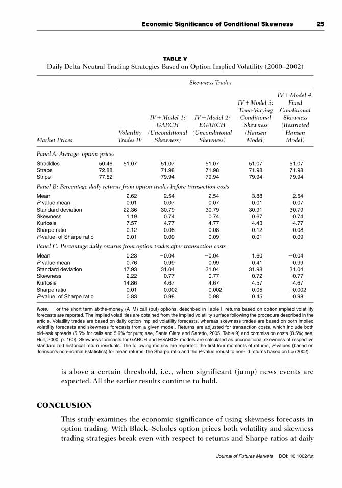
The model prices in Table V Panel A suggest that straddles are slightlyunderpriced in the market.12 Given that ATM puts (calls) are under (over)priced in the market by about $2.07 ($1.27) on average, strips (straps) areaccordingly under (over) priced on average.

Panel B, Table V, shows that the mean returns and Sharpe ratios are posi-tive and higher compared to Table III for all skewness trades before transactioncosts and significant at the 10% level. The skewness-based trades once againoutperform the straddle trades. Specifically, the time-varying conditional skew-ness (Hansen, 1994) model, i.e., model 3, along with IV results in the highestdaily returns of 3.88%. Model 3 also has the highest Sharpe ratio at 0.125.

Panel C shows that all strategies break even after including transactioncosts, and the Sharpe ratios are not significantly different from zero at the 5%level. Model 3 once again outperforms the straddle trades. Model 3 when com-bined with IVs clearly dominates historical volatility-based trades from TablesIII and IV. This implies that profits from daily skewness trades can be enhancedwith information from option IVs.13

Overall, conditional skewness model (Hansen, 1994) forecasts combinedwith option IVs deliver the best trading performance, and help minimize theloss exposure for an option trader trading in strips and straps. As before, the netoption profits still depend upon the underlying bid–ask spreads.

Further Robustness Tests

As further checks, alternative skewness trading strategies and skewness filtersare examined (results are not tabulated and available upon request). Skewnessfilters exclude noisy events and enable trades only when the skewness forecast

12The underpricing seems to mainly arise from ATM puts as the put IVs are upward biased, thereby leadingto somewhat high model prices (results not tabulated).13Untabulated results show that the incremental value from IV declines at weekly and monthly horizons.



is above a certain threshold, i.e., when significant (jump) news events areexpected. All the earlier results continue to hold.

CONCLUSION

This study examines the economic significance of using skewness forecasts inoption trading. With Black–Scholes option prices both volatility and skewnesstrading strategies break even with respect to returns and Sharpe ratios at daily

TABLE V

Daily Delta-Neutral Trading Strategies Based on Option Implied Volatility (2000–2002)

Skewness Trades

IV�Model 4:IV�Model 3: Fixed Time-Varying Conditional

IV�Model 1: IV�Model 2: Conditional Skewness GARCH EGARCH Skewness (Restricted

Volatility (Unconditional (Unconditional (Hansen Hansen Market Prices Trades IV Skewness) Skewness) Model) Model)

Panel A: Average option prices

Straddles 50.46 51.07 51.07 51.07 51.07 51.07Straps 72.88 71.98 71.98 71.98 71.98Strips 77.52 79.94 79.94 79.94 79.94

Panel B: Percentage daily returns from option trades before transaction costs

Mean 2.62 2.54 2.54 3.88 2.54P-value mean 0.01 0.07 0.07 0.01 0.07Standard deviation 22.36 30.79 30.79 30.91 30.79Skewness 1.19 0.74 0.74 0.67 0.74Kurtosis 7.57 4.77 4.77 4.43 4.77Sharpe ratio 0.12 0.08 0.08 0.12 0.08P-value of Sharpe ratio 0.01 0.09 0.09 0.01 0.09

Panel C: Percentage daily returns from option trades after transaction costs

Mean 0.23 �0.04 �0.04 1.60 �0.04P-value mean 0.76 0.99 0.99 0.41 0.99Standard deviation 17.93 31.04 31.04 31.98 31.04Skewness 2.22 0.77 0.77 0.72 0.77Kurtosis 14.86 4.67 4.67 4.57 4.67Sharpe ratio 0.01 �0.002 �0.002 0.05 �0.002P-value of Sharpe ratio 0.83 0.98 0.98 0.45 0.98

Note. For the short term at-the-money (ATM) call (put) options, described in Table I, returns based on option implied volatilityforecasts are reported. The implied volatilities are obtained from the implied volatility surface following the procedure described in thearticle. Volatility trades are based on daily option implied volatility forecasts, whereas skewness trades are based on both impliedvolatility forecasts and skewness forecasts from a given model. Returns are adjusted for transaction costs, which include bothbid–ask spreads (5.5% for calls and 5.9% for puts; see, Santa Clara and Saretto, 2005, Table 9) and commission costs (0.5%; see,Hull, 2000, p. 160). Skewness forecasts for GARCH and EGARCH models are calculated as unconditional skewness of respectivestandardized historical return residuals. The following metrics are reported: the first four moments of returns, P-values (based onJohnson’s non-normal t-statistics) for mean returns, the Sharpe ratio and the P-value robust to non-iid returns based on Lo (2002).



intervals, before including transaction costs. After transaction costs are fac-tored in, all strategies result in significant losses. The skewness-based tradesare, in general, less profitable compared to volatility trades. Further at weeklyor monthly intervals, there is no clear supportive evidence for skewness trades,both before and after transaction costs. When the Hull and White (1987)model is used, there is significant negative exposure across all trades and time-series models, with losses from volatility trades being substantially higher com-pared to the skewness-based trades. However, when the Corrado and Su(1996) model is used, the performance of skewness trades improves consider-ably, and skewness-based trades outperform the straddle trades. Finally, whentrades are implemented using the option IVs, skewness forecasts from the time-varying conditional skewness (Hansen, 1994) model deliver the best perform-ance at the daily trading horizon, based on average returns and Sharpe ratio,before and after trading costs.

The results indicate that a generalized option-pricing (Corrado & Su,1996, 1997) model can generate better trading performance for strip and straptrades. The evidence further implies that a generalized option-pricing model,along with forward-looking IVs and conditional skewness forecasts, can gener-ate a superior performance for skewness trades and help outperform the strad-dle trades.

Profitability of the trades are diluted by the high bid–ask spreads and fric-tions in the option market. The results are consistent with Santa-Clara andSaretto (2005), who show that the high returns in option strategies may nottranslate into profitable strategies after considering trading costs.

APPENDIX A: ROBUST STANDARD ERRORS FOR THE SHARPE RATIO

Sharpe ratio refers to the excess expected returns standardized by the underlyingrisk and is given by m � rf /s, where m and s are the expected return and risk,respectively, of the underlying exposure. The population Sharpe ratio S is estimat-ed from its sample moments as , where and refer to the samplemean and return standard deviation. The asymptotic distribution of the estimat-ed Sharpe ratio ( ) is described as (seeLo, 2002). Therefore, the standard error of the sample Sharpe ratio when theunderlying returns are IID is given by ,where T is the sam-ple size.

When the IID assumption is violated by the data, Lo (2002) derives the fol-lowing asymptotic expression for the estimate of standard error of Sharpe ratio(under the assumption of stationarity of returns): ,2T (S � S) �

aN(0, VGMM)

2(1 � 0.5 � S)�T

2T (S � S) �a

N(0, (1 � 0.5 � S2) )S

sm(m � rf)�s



where VGMM is the asymptotic variance based on GMM estimates of and .The standard error of the sample Sharpe ratio when the underlying returns are

non-IID is given by , where , ,

, and is the estimated variance obtained using the

Newey–West (1987) procedure.The GMM estimator of is given by the solution to ,

where . Once is obtained using GMM, the estimate

of VGMM and standard error of the sample Sharpe ratio can be calculated usingthe above expressions.

BIBLIOGRAPHY

Ait-Sahalia, Y., Wang, Y., & Yared, F. (2001). Do option markets correctly price theprobabilities of movement of the underlying asset? Journal of Econometrics, 102,67–110.

Bakshi, G., Cao, C., & Chen, Z. (1997). Empirical performance of alternative optionpricing models. Journal of Finance, 52, 2003–2049.

Bakshi, G., Kapadia, N., & Madan, D. (2003). Stock return characteristics, skew laws,and the differential pricing of individual equity options. Review of FinancialStudies, 16, 101–143.

Bates, D. S. (1996). Jumps and stochastic volatility: Exchange rate processes implicitin PHLX Deutschemark options. Review of Financial Studies, 9, 69–107.

Bates, D. S. (2000). Post-’87 crash fears in the S&P 500 futures option market. Journalof Econometrics, 94, 181–238.

Bekaert, G., & Wu, G. (2000). Asymmetric volatility and risk in equity markets. Reviewof Financial Studies, 13, 1–42.

Bollen N. P. B., & Whaley, R. E. (2004). Does net buying pressure affect the shape ofimplied volatility functions? Journal of Finance, 59, 711–753.

Bollerslev, T., & Mikkelsen, H. O. (1996). Modeling and pricing long memory in stockmarket volatility. Journal of Econometrics, 73, 151–184.

Brown, C. A., & Robinson, D. M. (2002). Skewness and kurtosis in S&P 500 indexreturns implied by option prices: A correction. Journal of Financial Research, 25,279–282.

Buraschi, A., & Jackwerth, J. C. (2001). The price of a smile: Hedging and spanning inoption markets. Review of Financial Studies, 14, 495–527.

Carr, P., & Wu, L. (2003). What type of process underlies options? A simple robust test.Journal of Finance, 58, 2581–2610.

Carr, P., & Wu, L. (2007). Stochastic skew for currency options. Journal of FinancialEconomics, 86, 213–247.

Chan, W., Jha, R., & Kalimipalli, M. (2009). The economic value of realized volatilityin forecasting implied volatility. Journal of Financial Research, forthcoming.

uwu(rf, u) � a Rt �m

(Rt�m)2 �s2b (1�T)aT

t�1wu(rf , u)�0u

©0g0u�

� a1�s(m � rf)�2s3b

u� a ms2bVGMM � (0g(u)�0u)©0g(u)�0u�2VGMM�T

sm



Chernov, M., & Ghysels, E. (2000). A study towards a unified approach to the jointestimation of objective and risk neutral measures for the purpose of options valua-tion. Journal of Financial Economics, 56, 407–458.

Christoffersen, P. (2003). Elements of financial risk management. San Diego, CA:Academic Press.

Christoffersen, P., Heston, S. L., & Jacobs, K. (2006). Option valuation with condi-tional skewness. Journal of Econometrics, 131, 253–284.

Christoffersen, P., & Jacobs, K. (2004). The importance of the loss function in optionvaluation. Journal of Financial Economics, 72, 291–318.

Constantinides, G. M., Jackwerth, J. C., & Perrakis, S. (2009). Mispricing of S&P 500index options, Review of Financial Studies, 22, 1247–1277.

Corrado, C. J., & Su, T. (1996). Skewness and kurtosis in S&P 500 index returnsimplied by option prices. Journal of Financial Research, 19, 175–192.

Corrado, C. J., & Su, T. (1997). Implied volatility skews and stock index skewness andkurtosis implied by S&P 500 index option prices. Journal of Derivatives, Summer,8–19.

Coval, J. D., & Shumway T. (2001). Expected option returns. Journal of Finance, 56,983–1009.

Das, S. R., & Sundaram, R. K. (1999). Of smiles and smirks: A term structure perspec-tive. Journal of Financial and Quantitative Analysis, 34, 211–239.

Dennis, P., & Mayhew, S. (2002). Risk-neutral skewness: Evidence from index options.Journal of Financial and Quantitative Analysis, 37, 471–493.

Dittmar, R. F. (2002). Nonlinear pricing kernels, kurtosis preference, and evidence ofthe cross section of equity returns. Journal of Finance, 57, 369–403.

Dumas, B., Fleming J., & Whaley R. E. (1998). Implied volatility functions: Empiricaltests. Journal of Finance, 53, 2059–2106.

Eraker, B. (2004). Do stock prices and volatility jump? Reconciling evidence from spotand option prices. Journal of Finance, 14, 1367–1403.

Eraker, B., Johannes, M., & Polson, N. (2003). The impact of jumps in volatility andreturns. Journal of Finance, 58, 1269–1300.

Figlewski, S. (1989). Options arbitrage in imperfect markets. Journal of Finance, 44,1289–1311.

Giot, P., & Laurent, S. (2003). Value-at-risk for long and short positions. Journal ofApplied Econometrics, 18, 641–664.

Hansen, B. E. (1994). Autoregressive conditional density estimation. InternationalEconomic Review, 35, 705–730.

Harvey, C. R., & Siddique, A. (1999). Autoregressive conditional skewness. Journal ofFinancial and Quantitative Analysis, 34, 465–487.

Harvey, C. R., & Siddique, A. (2000). Conditional skewness in asset pricing tests.Journal of Finance, 55, 1263–1295.

Heston, S. (1993). A closed form solution with options with stochastic volatility, withapplications to bond and currency markets. Review of Financial Studies, 6,327–343.

Heston, S., & Nandi, S. (2000). A closed-form GARCH option valuation model.Review of Financial Studies, 13, 585–625.

Hull, J. (2000). Options, futures, and other derivatives (4th ed.). New Jersey: Prentice-Hall.



Hull, J., & Suo, W. (2002). A methodology for assessing model risk and its applicationto the implied volatility function model. Journal of Financial and QuantitativeAnalysis, 37, 297–318.

Hull, J., & White, A. (1987). The pricing of options on assets with stochastic volatili-ties. Journal of Finance, 42, 281–300.

Jackwerth, J. C. (2000). Recovering risk aversion from and realized returns. Review ofFinancial Studies, 13, 433–451.

Jiang, G. J., & Tian, Y. S. (2005). Model free implied volatility and its information con-tent. Review of Financial Studies, 18, 1305–1342.

Johnson, N. J. (1978). Modified t-tests and confidence intervals for asymmetric popu-lations. Journal of the American Statistical Association, 73, 536–544.

Jondeau, E., & Rockinger, M. (2003). Conditional volatility, skewness, and kurtosis:Existence, persistence and comovements. Journal of Economic Dynamics &Control, 27, 1699–1737.

Jones, C. (2003). The dynamics of stochastic volatility: Evidence from underlying andoptions markets. Journal of Econometrics, 116, 181–224.

Lehnert, T. (2003). Explaining smiles: GARCH option pricing with conditionalleptokurtosis and skewness. Journal of Derivatives, 10, 27–39.

Lim, G. C., Martin, G. M., & Martin, V. L. (2005). Parametric pricing of higher ordermoments in S&P500 options. Journal of Applied Econometrics, 20, 377–404.

Lim, G. C., Martin, G. M., & Martin, V. L. (2006). Pricing currency options in thepresence of time-varying volatility and non-normalities. Journal of MultinationalFinancial Management, 16, 291–314.

Lo, A. (2002). Statistics of Sharpe ratios. Financial Analysts Journal, 58, 36–52.Martin, G. M., Forbes, C. S., & Martin, V. L. (2005). Implicit Bayesian inference using

option prices. Journal of Time Series Analysis, 26, 427–462.Nandi, S. (1998). How important is the correlation between returns and volatility in a

stochastic volatility model? Empirical evidence from pricing and hedging in theS&P 500 index option market. Journal of Banking & Finance, 22, 589–610.

Newey, W. K., & West, K. D. (1987). A simple positive definite heteroskedasticity andautocorrelation consistent covariance matrix. Econometrica, 55, 703–708.

Noh, J., Engle R., & Kane A. (1994). Forecasting volatility and option prices of the S&Pindex. Journal of Derivatives, Fall, 17–30.

Pan, J. (2002). The jump-risk premia implicit in options: Evidence from an integratedtime-series study. Journal of Financial Economics, 63, 3–50.

Patton, A. J. (2004). On the out-of-sample importance of skewness and asymmetricdependence for asset allocation. Journal of Financial Econometrics, 2, 130–168.

Santa-Clara, P., & Saretto, A. (2005). Option strategies: Good deals and margin calls(working paper). UCLA.

Vuong, Q. (1989). Likelihood ratio tests for model selection and non-nested hypothesis.Econometrica, 57, 307–333.

The economic significance of conditional skewness in index option markets

Documents

Transcript of The economic significance of conditional skewness in index option markets