Unit-III Measures of Dispersion & Skewness CONTENTS ...
42
Unit-III Measures of Dispersion & Skewness CONTENTS Measures of Dispersion 2.1 Range 2.2 Quartile Deviation (Q.D) 2.3 Standard Deviation 2.3.1 Combined Standard Deviation: 2.4 Mean Deviation OR Average Deviation 2.4.1 Difference between the Mean Deviation and standard Deviation 2.5 Coefficient of Variation 2.6 Variance 2.7 Skewness 2.7.1 Karl- Pearson’s Coefficient of Skewness 2.7.2 Bowley’s Coefficient of Skewness Measures of Dispersion Definition: It is hardly fully representative of a mass, unless we know the manner in which the individual items scatter around it. A further description of the series is necessary if we are to gauge how representative the average is. .
-
Upload
khangminh22 -
Category
Documents
-
view
1 -
download
0
Transcript of Unit-III Measures of Dispersion & Skewness CONTENTS ...
Unit-III
Measures of Dispersion & Skewness
CONTENTS
Measures of Dispersion
2.1 Range
2.2 Quartile Deviation (Q.D)
2.3 Standard Deviation
2.3.1 Combined Standard Deviation:
2.4 Mean Deviation OR Average Deviation
2.4.1 Difference between the Mean Deviation
and standard Deviation
2.5 Coefficient of Variation
2.6 Variance
2.7 Skewness
2.7.1 Karl- Pearson’s Coefficient of Skewness
2.7.2 Bowley’s Coefficient of Skewness
Measures of Dispersion
Definition: It is hardly fully representative of a mass, unless we know the manner in which the
individual items scatter around it. A further description of the series is necessary if we are to gauge
how representative the average is.
.

Importance or Significance of Measures of Dispersion:
The reliability of a measure of central tendency is known.
1. Measures of Dispersion provide a basis for the control of variability.
2. They help to compare two or more sets of data with regard to their variability.
3. They enhance the utility and scope of statistical techniques.
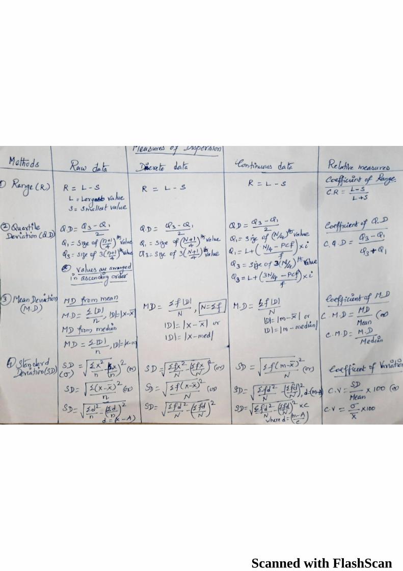
The Usual Measures of Dispersion: The usual measures of dispersion, very often suggested by the statisticians, are exhibited
with the aid of the following chart:
Difference between the Absolute measure and Relative Measure:
Absolute measure Relative measure
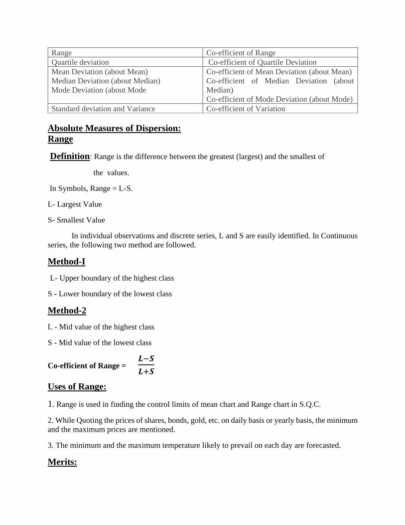
Range Co-efficient of Range
Quartile deviation Co-efficient of Quartile Deviation
Mean Deviation (about Mean)
Median Deviation (about Median)
Mode Deviation (about Mode
Co-efficient of Mean Deviation (about Mean)
Co-efficient of Median Deviation (about
Median)
Co-efficient of Mode Deviation (about Mode)
Standard deviation and Variance Co-efficient of Variation
Absolute Measures of Dispersion:
Range
Definition: Range is the difference between the greatest (largest) and the smallest of
the values.
In Symbols, Range = L-S.
L- Largest Value
S- Smallest Value
In individual observations and discrete series, L and S are easily identified. In Continuous
series, the following two method are followed.
Method-I
L- Upper boundary of the highest class
S - Lower boundary of the lowest class
Method-2
L - Mid value of the highest class
S - Mid value of the lowest class
Co-efficient of Range = 𝑳−𝑺
𝑳+𝑺
Uses of Range:
1. Range is used in finding the control limits of mean chart and Range chart in S.Q.C.
2. While Quoting the prices of shares, bonds, gold, etc. on daily basis or yearly basis, the minimum
and the maximum prices are mentioned.
3. The minimum and the maximum temperature likely to prevail on each day are forecasted.
Merits:
1. It is simple to understand and easy to calculate.
2. It can be calculated in no time.
Demerits:
1. Its definition does not seem to suit continuous series.
2. It is based on the two extreme items. It does not consider the other items.
3. It is usually affected by the extreme items.
4. It cannot be manipulated algebraically. The Range of combined set cannot be found from
the range of the individual sets.
5. It does not have sampling stability.
6. It cannot be calculated from open-end class intervals. It is a very rarely used measure. Its
Scope is limited.
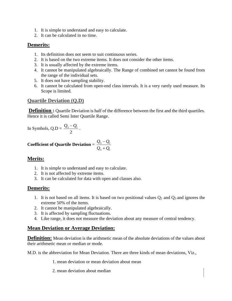
Quartile Deviation (Q.D)
Definition : Quartile Deviation is half of the difference between the first and the third quartiles.
Hence it is called Semi Inter Quartile Range.
In Symbols, Q.D = 2
13 QQ −.
Coefficient of Quartile Deviation = 13
13
+
−
Merits:
1. It is simple to understand and easy to calculate.
2. It is not affected by extreme items.
3. It can be calculated for data with open and classes also.
Demerits:
1. It is not based on all items. It is based on two positional values Q1 and Q3 and ignores the
extreme 50% of the items.
2. It cannot be manipulated algebraically.
3. It is affected by sampling fluctuations.
4. Like range, it does not measure the deviation about any measure of central tendency.
Mean Deviation or Average Deviation:
Definition: Mean deviation is the arithmetic mean of the absolute deviations of the values about
their arithmetic mean or median or mode.
M.D. is the abbreviation for Mean Deviation. There are three kinds of mean deviations, Viz.,
1. mean deviation or mean deviation about mean
2. mean deviation about median
3. mean deviation about mode.
Mean deviation about median is the least. it could be easily verified in individual observations and
discrete series where the actual values are considered.
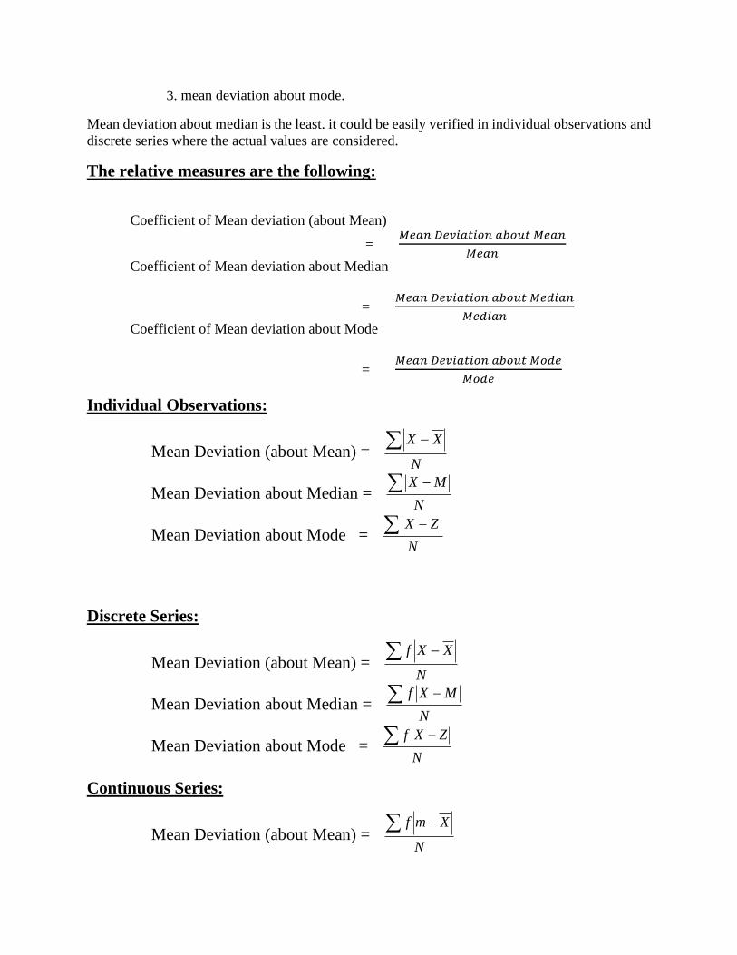
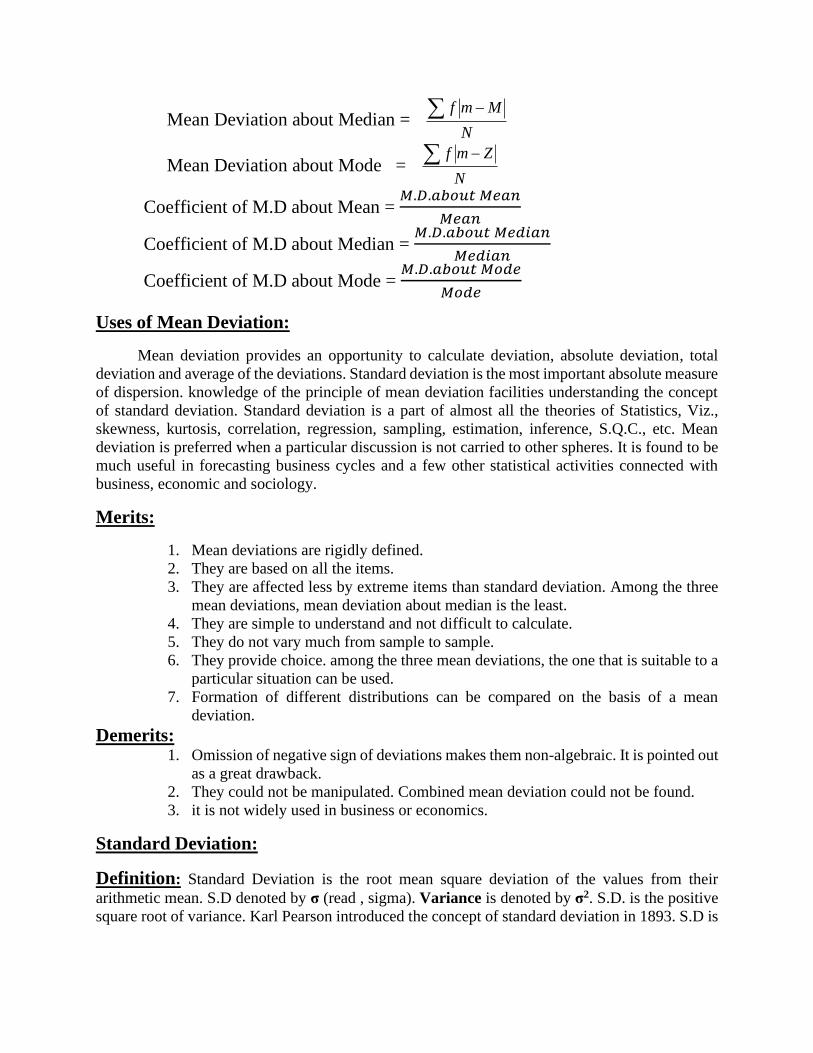
The relative measures are the following:
Coefficient of Mean deviation (about Mean)
= 𝑀𝑒𝑎𝑛 𝐷𝑒𝑣𝑖𝑎𝑡𝑖𝑜𝑛 𝑎𝑏𝑜𝑢𝑡 𝑀𝑒𝑎𝑛
𝑀𝑒𝑎𝑛
Coefficient of Mean deviation about Median
= 𝑀𝑒𝑎𝑛 𝐷𝑒𝑣𝑖𝑎𝑡𝑖𝑜𝑛 𝑎𝑏𝑜𝑢𝑡 𝑀𝑒𝑑𝑖𝑎𝑛
𝑀𝑒𝑑𝑖𝑎𝑛
Coefficient of Mean deviation about Mode
= 𝑀𝑒𝑎𝑛 𝐷𝑒𝑣𝑖𝑎𝑡𝑖𝑜𝑛 𝑎𝑏𝑜𝑢𝑡 𝑀𝑜𝑑𝑒
𝑀𝑜𝑑𝑒
Individual Observations:
Mean Deviation (about Mean) = N
XX −
Mean Deviation about Median = N
MX −
Mean Deviation about Mode = N
ZX −
Discrete Series:
Mean Deviation (about Mean) = N
XXf −
Mean Deviation about Median = N
MXf −
Mean Deviation about Mode = N
ZXf −
Continuous Series:
Mean Deviation (about Mean) = N
Xmf −
Mean Deviation about Median = N
Mmf −
Mean Deviation about Mode = N
Zmf −
Coefficient of M.D about Mean = 𝑀.𝐷.𝑎𝑏𝑜𝑢𝑡 𝑀𝑒𝑎𝑛
𝑀𝑒𝑎𝑛
Coefficient of M.D about Median = 𝑀.𝐷.𝑎𝑏𝑜𝑢𝑡 𝑀𝑒𝑑𝑖𝑎𝑛
𝑀𝑒𝑑𝑖𝑎𝑛
Coefficient of M.D about Mode = 𝑀.𝐷.𝑎𝑏𝑜𝑢𝑡 𝑀𝑜𝑑𝑒
𝑀𝑜𝑑𝑒
Uses of Mean Deviation:
Mean deviation provides an opportunity to calculate deviation, absolute deviation, total
deviation and average of the deviations. Standard deviation is the most important absolute measure
of dispersion. knowledge of the principle of mean deviation facilities understanding the concept
of standard deviation. Standard deviation is a part of almost all the theories of Statistics, Viz.,
skewness, kurtosis, correlation, regression, sampling, estimation, inference, S.Q.C., etc. Mean
deviation is preferred when a particular discussion is not carried to other spheres. It is found to be
much useful in forecasting business cycles and a few other statistical activities connected with
business, economic and sociology.
Merits:
1. Mean deviations are rigidly defined.
2. They are based on all the items.
3. They are affected less by extreme items than standard deviation. Among the three
mean deviations, mean deviation about median is the least.
4. They are simple to understand and not difficult to calculate.
5. They do not vary much from sample to sample.
6. They provide choice. among the three mean deviations, the one that is suitable to a
particular situation can be used.
7. Formation of different distributions can be compared on the basis of a mean
deviation.
Demerits: 1. Omission of negative sign of deviations makes them non-algebraic. It is pointed out
as a great drawback.
2. They could not be manipulated. Combined mean deviation could not be found.
3. it is not widely used in business or economics.
Standard Deviation:
Definition: Standard Deviation is the root mean square deviation of the values from their
arithmetic mean. S.D denoted by σ (read , sigma). Variance is denoted by σ2. S.D. is the positive
square root of variance. Karl Pearson introduced the concept of standard deviation in 1893. S.D is
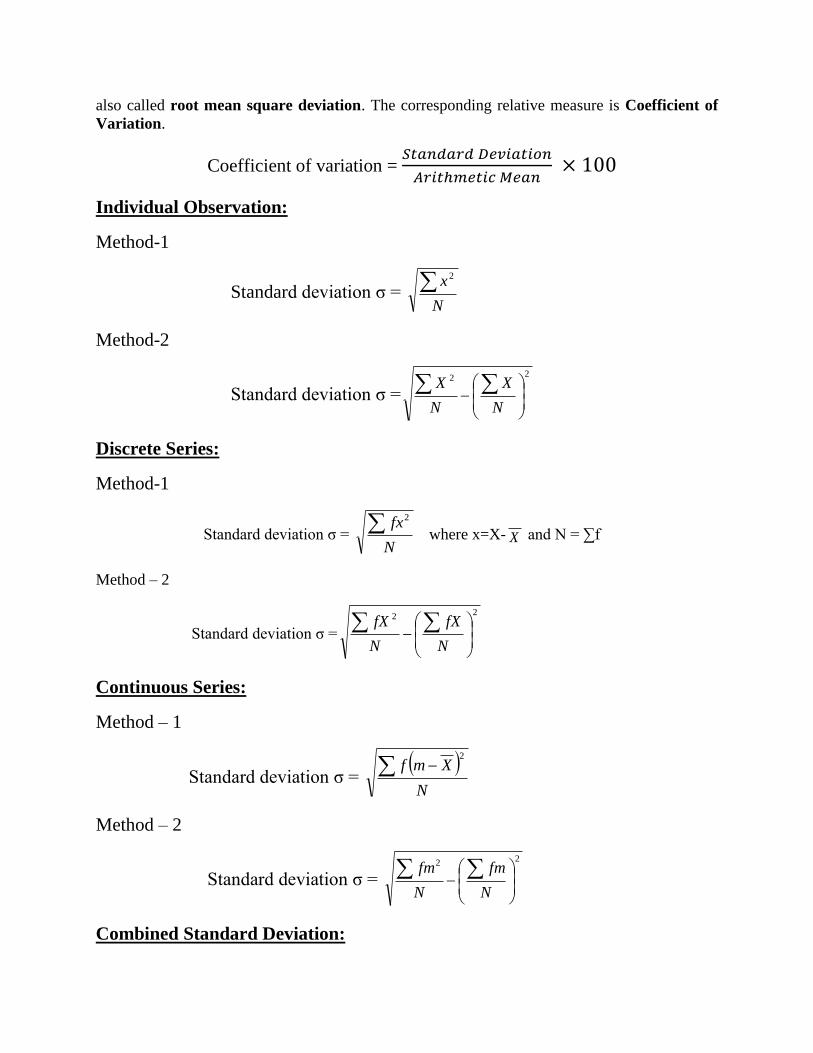
also called root mean square deviation. The corresponding relative measure is Coefficient of
Variation.
Coefficient of variation = 𝑆𝑡𝑎𝑛𝑑𝑎𝑟𝑑 𝐷𝑒𝑣𝑖𝑎𝑡𝑖𝑜𝑛
𝐴𝑟𝑖𝑡ℎ𝑚𝑒𝑡𝑖𝑐 𝑀𝑒𝑎𝑛 × 100
Individual Observation:
Method-1
Standard deviation σ = N
x 2
Method-2
Standard deviation σ =
22
−
N
X
N
X
Discrete Series:
Method-1
Standard deviation σ = N
fx 2
where x=X- X and N = ∑f
Method – 2
Standard deviation σ =
22
−
N
fX
N
fX
Continuous Series:
Method – 1
Standard deviation σ = ( )N
Xmf −2
Method – 2
Standard deviation σ =
22
−
N
fm
N
fm
Combined Standard Deviation:
When two or three groups merge, the mean and standard deviation of the combined group are
calculated as follows.
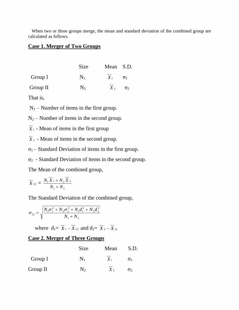
Case 1. Merger of Two Groups
Size Mean S.D.
Group I N1 1X σ1
Group II N2 2X σ2
That is,
N1 – Number of items in the first group.
N2 – Number of items in the second group.
1X - Mean of items in the first group
2X - Mean of items in the second group.
σ1 – Standard Deviation of items in the first group.
σ2 - Standard Deviation of items in the second group.
The Mean of the combined group,
12X = 21
2211
NN
XNXN
+
+
The Standard Deviation of the combined group,
21
2
22
2
11
2
22
2
1112
NN
dNdNNN
+
+++=
where d1= 121 XX − and d2= 122 XX −
Case 2. Merger of Three Groups
Size Mean S.D.
Group I N1 1X σ1
Group II N2 2X σ2
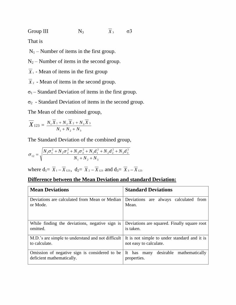
Group III N3 3X σ3
That is
N1 – Number of items in the first group.
N2 – Number of items in the second group.
1X - Mean of items in the first group
2X - Mean of items in the second group.
σ1 – Standard Deviation of items in the first group.
σ2 - Standard Deviation of items in the second group.
The Mean of the combined group,
123X = 321
332211
NNN
XNXNXN
++
++
The Standard Deviation of the combined group,
321
2
33
2
22
2
11
2
33
2
22
2
11
12NNN
dNdNdNNNN
++
+++++=
where d1= 1231 XX − , d2= 1232 XX − and d3= 1233 XX −
Difference between the Mean Deviation and standard Deviation:
Mean Deviations Standard Deviations
Deviations are calculated from Mean or Median
or Mode.
Deviations are always calculated from
Mean.
While finding the deviations, negative sign is
omitted.
Deviations are squared. Finally square root
is taken.
M.D.’s are simple to understand and not difficult
to calculate.
It is not simple to under standard and it is
not easy to calculate.
Omission of negative sign is considered to be
deficient mathematically.
It has many desirable mathematically
properties.
Uses
Standard deviation is the best absolute measure of dispersion. It is a part of many statistical
concepts such as Skewness, Kurtosis, Correlation, Regression, Estimation, sampling, tests of
Significance and Statistical Quality Control. Not only in statistics but also in Biology, education,
Psychology and other disciplines standard deviation is of immense use.
Merits:
1. Standard deviation is rigidly defined.
2. It is calculated on the basis of the magnitudes of all the items.
3. It could be manipulated further. The combined S.D. can be calculated.
4. Mistakes in its calculation can be corrected. The entire calculation need not be redone.
5. Coefficient of variation is based on S.D.. It is the best and most widely used relative
measure of dispersion.
6. It is free from sampling fluctuations. This property of sampling stability has brought it an
indispensable place in tests of significance.
7. It reduces the complexity in the approach of normal distribution by providing standard
normal variable.
8. It is the most important absolute measure of dispersion. It is used in all the areas of
statistics. It is widely used in other disciplines such as Psychology, Education and Biology
as well.
9. Scientific calculators show the standard deviation of any series.
10. Different forms of the formula are available.
Demerits:
1. Compared with other absolute measures of dispersion, it is difficult to calculate.
2. It is not simple to understand.
3. It gives more weight age to the items away from the mean than those near the mean as the
deviations are squared.
Coefficient of Variation
Definition: Coefficient of variation is the most widely used relative measure of dispersion. It is
based on the best absolute measure of dispersion and the best measure of central tendency. It is a
percentage. While comparing two or more groups, the group which has less coefficient of variation
is less variable or more consistent or more stable or more uniform or more homogeneous.
Coefficient of Variation is denoted by the C.V.
Coefficient of Variation = 𝑆𝑡𝑎𝑛𝑑𝑎𝑟𝑑 𝐷𝑒𝑣𝑖𝑎𝑡𝑖𝑜𝑛
𝐴𝑟𝑖𝑡ℎ𝑚𝑒𝑡𝑖𝑐 𝑀𝑒𝑎𝑛× 100
C.V. = 𝑆.𝐷.
𝐴.𝑀.× 100 OR C.V. = 100
X
Variance
Variance is the mean square deviation of the values from their arithmetic mean. It is denoted
by σ2. Standard deviation is the positive square root of variance and is denoted by σ. The term of
variance was introduced by R.A. fisher in the year 1913. It is used much in sampling, analysis of
variance, etc., In analysis of variance, total variation is split into a few components. Each
component is ascribable to one factor of variation. The significance of the variation is then tested.
Individual Observation:
Variance, σ2 = ( )
N
XX −2
Discrete Series:
Variance, σ2 =
22
−
N
fX
N
fX
Continuous Series:
Variance, σ2 =
−
222
2''
N
fd
N
dC
Combined Variance:
Based on the notations used in combined mean and combined variance,
Combined variance of two groups,
21
2
22
2
11
2
22
2
112
12NN
dNdNNN
+
++++=
Combined variance of three groups,
321
2
33
2
22
2
11
2
33
2
22
2
112
123NNN
dNdNdNNNN
++
+++++=
Skewness:
Definition: Skewness is the degree of asymmetry, or departure from symmetry, of a
distribution.
There are two types of Skewness: Positive and Negative
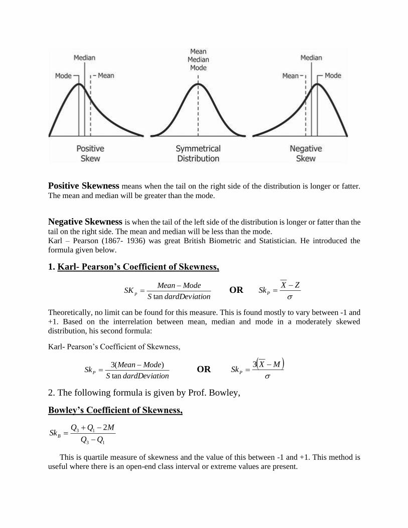
Positive Skewness means when the tail on the right side of the distribution is longer or fatter.
The mean and median will be greater than the mode.
Negative Skewness is when the tail of the left side of the distribution is longer or fatter than the
tail on the right side. The mean and median will be less than the mode.
Karl – Pearson (1867- 1936) was great British Biometric and Statistician. He introduced the
formula given below.
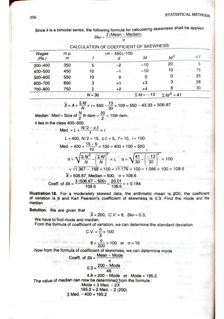
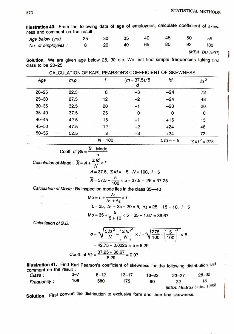
1. Karl- Pearson’s Coefficient of Skewness,
iondardDeviatS
ModeMeanSK p
tan
−= OR
ZXSkP
−=
Theoretically, no limit can be found for this measure. This is found mostly to vary between -1 and
+1. Based on the interrelation between mean, median and mode in a moderately skewed
distribution, his second formula:
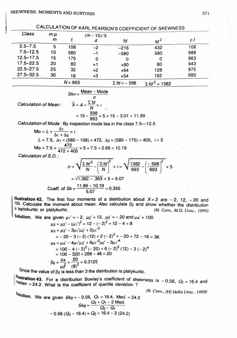
Karl- Pearson’s Coefficient of Skewness,
iondardDeviatS
ModeMeanSkP
tan
)(3 −= OR
( )
MXSkP
−=
3
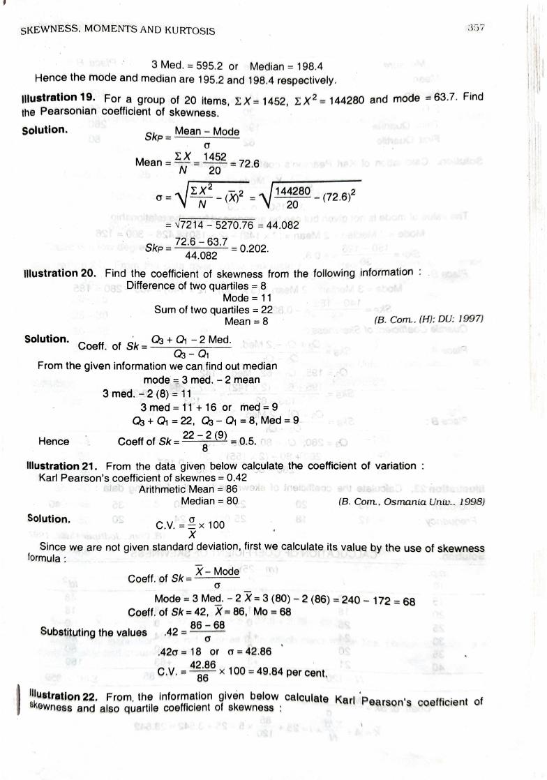
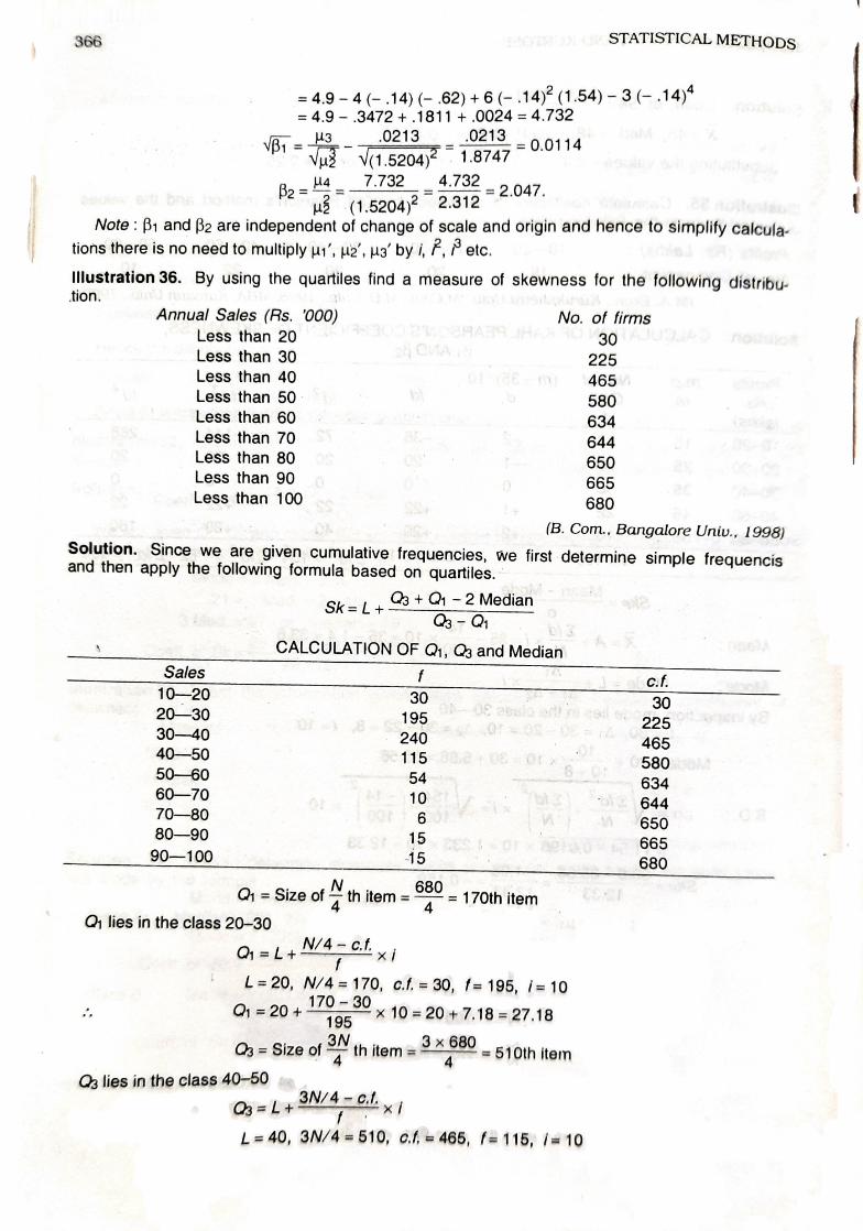
2. The following formula is given by Prof. Bowley,
Bowley’s Coefficient of Skewness,
13
13 2
MQQSkB
−
−+=
This is quartile measure of skewness and the value of this between -1 and +1. This method is
useful where there is an open-end class interval or extreme values are present.

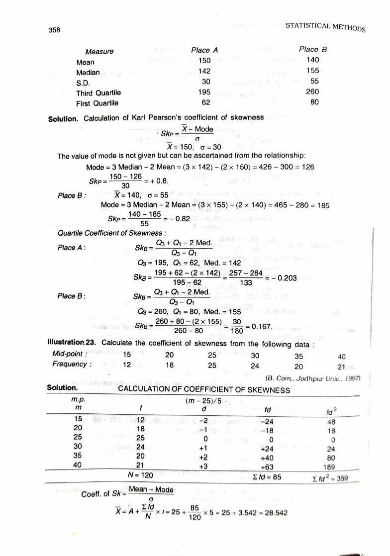
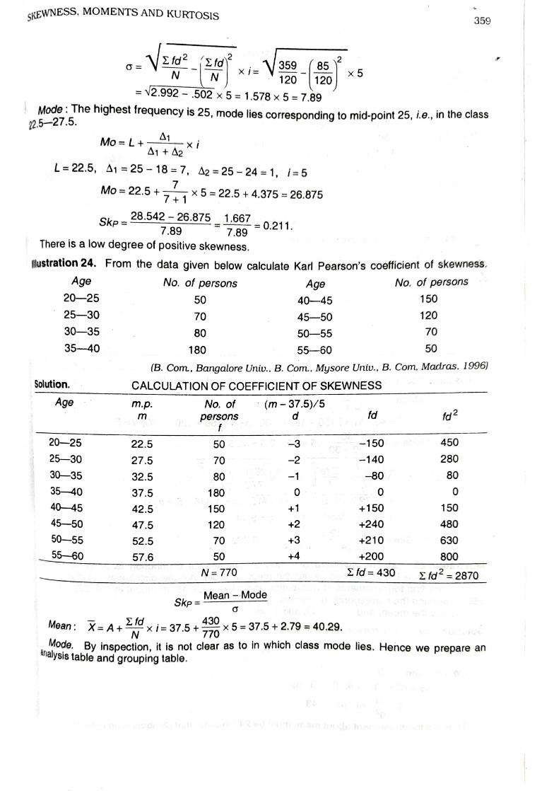
MEASURES OF DISPERSION 271
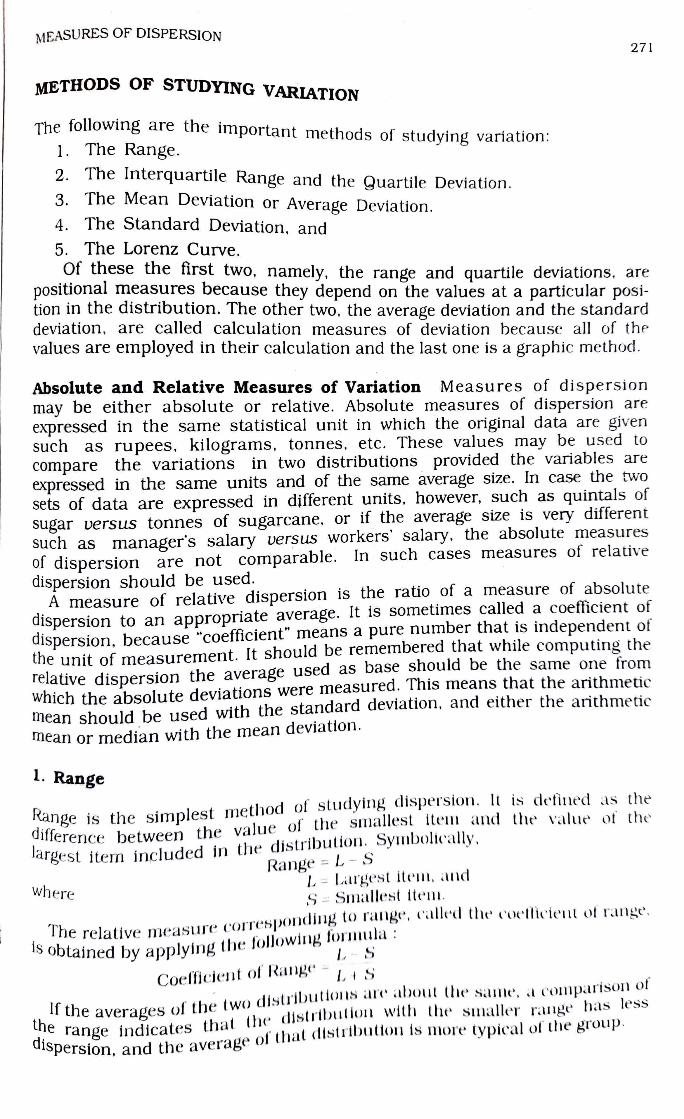
METHODS OF STUDYING VARIATION
The following are the important methods of studying variation: 1. The Range.
2. The Interquartile Range and the Quartile Deviatiorn.3. The Mean Deviation or Average Deviation. 4. The Standard Deviation, and
5. The Lorenz Curve. Of these the first two, namely, the range and quartile deviations. are
positional measures because they depend on the values at a particular posi- tion in the distribution. The other two, the average deviation and the standard deviation, are called calculation measures of deviation because all of the values are employed in their calculation and the last one is a graphic method.
Absolute and Relative Measures of Variation Measures of dispersion may be either absolute or relative. Absolute measures of dispersion are expressed in the same statistical unit in which the original data are given such as rupees, kilograms, tonnes. etc. These values may be used to
Compare expressed in the same units and of the same average size. In case the twvo
sets of data are expressed in different units. however, such as quintals of
sugar versus tonnes of sugarcane, or if the average size is very different
Such aS manager's salary versus workers salary, the absolute measures
of dispersion
dispersion should be used.
A measure of relative dispersion is the ratio of a measure of absolute
dispersion to an appropriate average. It is sometimes called a coefficient of
dispersion, because "coefficient" means a pure number that is independent of
the unit of measurement. It should be remembered that while computing the
relative dispersion the average used as base should be the same one from
which the absolute deviations were measured. This means that the arithmetic
mean should be used with the standard deviation, and either the arithmetic
nean or median with the mean deviatlon.
the variations in two distributions provided the variables are
are not comparable. In such cases measures of relative
1. Range
ange is the simplest method of sludying dispersion. lt is detined as the
ifference between the value oI the smallest ilem and the value of the
largest item included in the distribution. Syinbolically, Range L- S
L = Largest ite, and
where S Sallest item.
The relative measure corresponing
to rallge, caled the coetlicien ot range
ODtained by applying the following forula
-S
Coefficient of Range LS
the averages of the two distriDutols ale boul the saune, a coparison of
range indicates that the distribuo11 With the smaller range has less
spersion, and the average of thal distridutton is nore typical of the group.
STATISTCAL METHODS 272
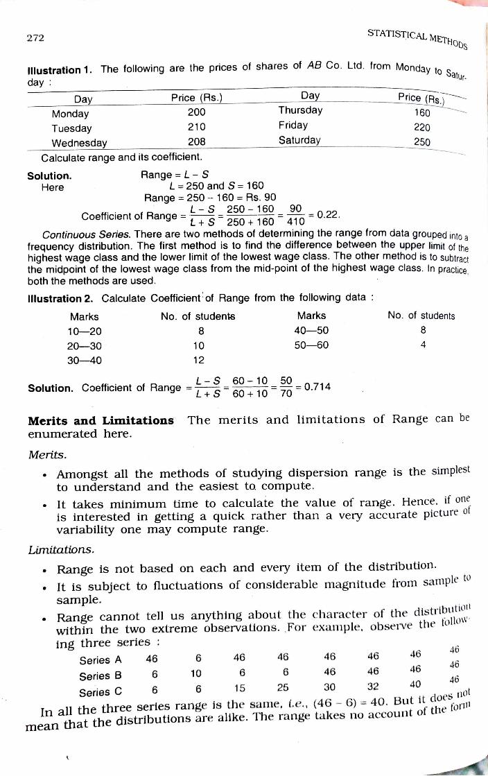
llustration 1. The following are the prices of shares of AB Co. Ltd. from Mondav
lay ay to Satur
Price (Rs.) Day Price (Rs.) Day Monday 200 Thursday 160
Tuesday 210 Friday 220 208 Saturday 250 Wednesday
Calculate range and its coefficient.
Solution. Here
Range L- S L= 250 and S = 160
Range 250 160 = Rs. 90
Coefficient of Range = S 250- 160 L+ S 250+ 160 90-0.22.410
Continuous Series. There are two methods of determining the range from data grouped into a frequency distribution. The first method is to find the difference between the upper limit of the highest wage class and the lower limit of the lowest wage class. The other method is to subtract the midpoint of the lowest wage class from the mid-point of the highest wage class. In practice,
both the methods are used.
Illustration 2. Calculate Coefficient of Range from the following data
Marks No. of students Marks No. of students
10-20 8 40-50 8
20-30 10 50-60 4
30-40 12
50 Solution. Coefficient of Range 10700.714
The merits and limitations of Range can be Merits and Limitations enumerated here.
Merits.
. Amongst all the methods of studying dispersion range is the simplest to understand and the easiest to compute.
. It takes minimum time to calculate the value of range. Hence. it on is interested in getting a quick rather than a very accurate picture o variability one may compute range.
Limitations.
Range is not based on each and every item of the distribution.
It is subject to fluctuations of considerable magnitude from sample
sample.
Range cannot tell us anything about the character of the distribuowithin the two extreme observations. For example. ing three series
Observe the tollow
46 Series A 46 6 46 46 46 46 46
46 6 10 6 6 46 46 46
Series B 46 6 6 15 25 30 32 40
Series C
In all the three series range is the same, i.e., (46 6) = 40. But it does
mean that the distributions are allke. The range takes no account of the fol"
STATISTICAL METHODS 274
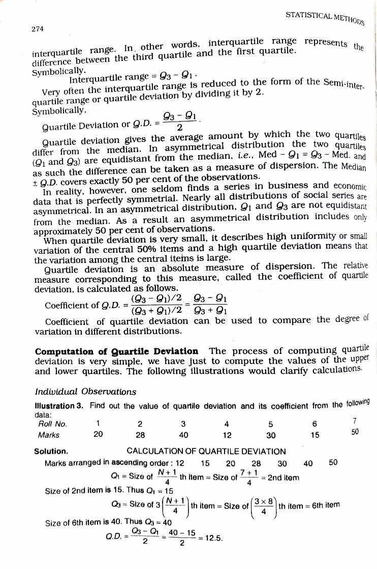
interquartile range. In. other words, interquartile range rep
difference between the third quartile and the first quartile.
Symbolically.
range represents the
Interquartile range = 93- 91
Very often the interquartile range is reduced to the form of the Semi.:
quartile range or quartile deviation by dividing it by 2.
Symbolically.
Semi-inter-
Quartile Deviation or Q.D. = 391
Quartile deviation gives the average amount by which the two quartil
differ from the median. In asymmetrical distribution the two quartil
(O1 and 93) are equidistant from the median, Le., Med - 91 = 93 Med. and
as such the difference can be taken as a measure of dispersion. The Median
t9.D. covers exactly 50 per cent of the observations.
In reality, however, one seldom finds a series in business and economic
data that is perfectly symmetrial. Nearly all distributions of social series are
asymmetrical. In an asymmetrical distribution, O1 and 93 are not equidistant
from the median. As a result an asymmetrical distribution includes only
approximately 50 per cent of observationS.
When quartile deviation is very small, it describes high uniformity or small
variation of the central 50% items and a high quartile deviation means that
the variation among the central items is large.
Quartile deviation is an absolute measure of dispersion. The relative measure corresponding to this measure, called the coefficient of quartile
deviation, is calculated as follows.
2
D. =
(93- O1)/2 O3-91 Coefficient of Q.D. 93+91)/2 O3+91 Coefficient of quartile deviation can be used to compare the degree ot
variation in different distributions.
Computation of guartile Deviation The process of computing quar deviation is very simple, we have just to compute the values of the upre and lower quartiles. The following illustrations would clarify calculauon
Indiwidual Observations Ilustration 3. Find out the value of quartile deviation and its coefficient from the follow data:
7 Roll No
Marks 1 2 3 4 5 6
20 28 40 12 30 15 50
Solution. CALCULATION OF QUARTILE DEVIATION Marks arranged in ascending order: 12 15 20 28 30 40 50
O Size of th item Size of =2nd item 4 4
Size of 2nd item is 15. Thus Q = 15
Gs Size of 3 th item Size of th item= 6th item
Size of 6th item is 40. Thus Q = 40
Q.D. = 40-15 12.5. 2 2
275 MEASURES OF DISPERSION
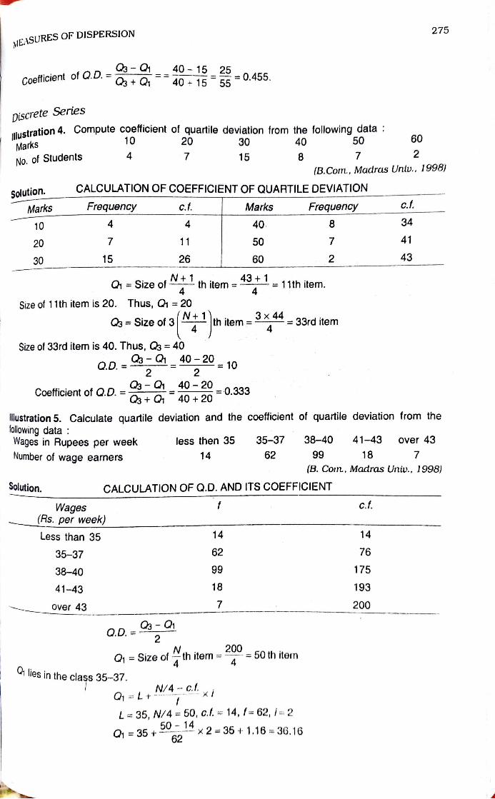
Coefficient of Q.D. :
Qa + 40-15_23-0.455. 40+ 15 55 0.455.
Discrete Series
uk stration 4. Compute coefficient of quartile deviation from the following data 20 10 30 40 50 60
Marks
4 7 15 8 2 No. of Students
(B.Com., Madras Untv., 1998)
CALCULATION OF COEFFICIENT OF QUARTILE DEVIATION Solution.
Marks FrequencyY C.f. Marks Frequency C.f.
10 40 8 34
20 7 11 50 41
30 15 26 60 2 43
a= Size of th item =4 = 11th item. 4
Size of 11th item is 20. Thus, Q1 20
Os Size of 3 th item =x4= 33rd item
Size of 33rd item is 40. Thus, Qa= 40 QD 3-_40-20 10
2 2
Coefficient oft Q.D. - = 0.333 O3+O 40 + 20
llustration 5. Calculate quartile deviation and the coefficient of quartile deviation from the
following data Wages in Rupees per week Number of wage earners
less then 35 35-37 38-40 41-43 over 43
14 62 99 18 7
(B. Con., Madras Uniw., 1998)
Solution. CALCULATION OF Q.D. AND ITS COEFFICIENT
C.f. Wages Rs. per week)
Less than 35 14 14
35-37 62 76
38-40 99 175
41-43 18 193
Over 43 200
Q.D. = -O
200 O Size ofth item- 50 th iten
4
lies in the cla_s 35-37 N/4-C.xi Q1 = L+
L 35, N/4 = 50, c.f, = 14, f= 62, /= 2
Q 35+ b0 14 x2 -35 + 1.16 36.16 62
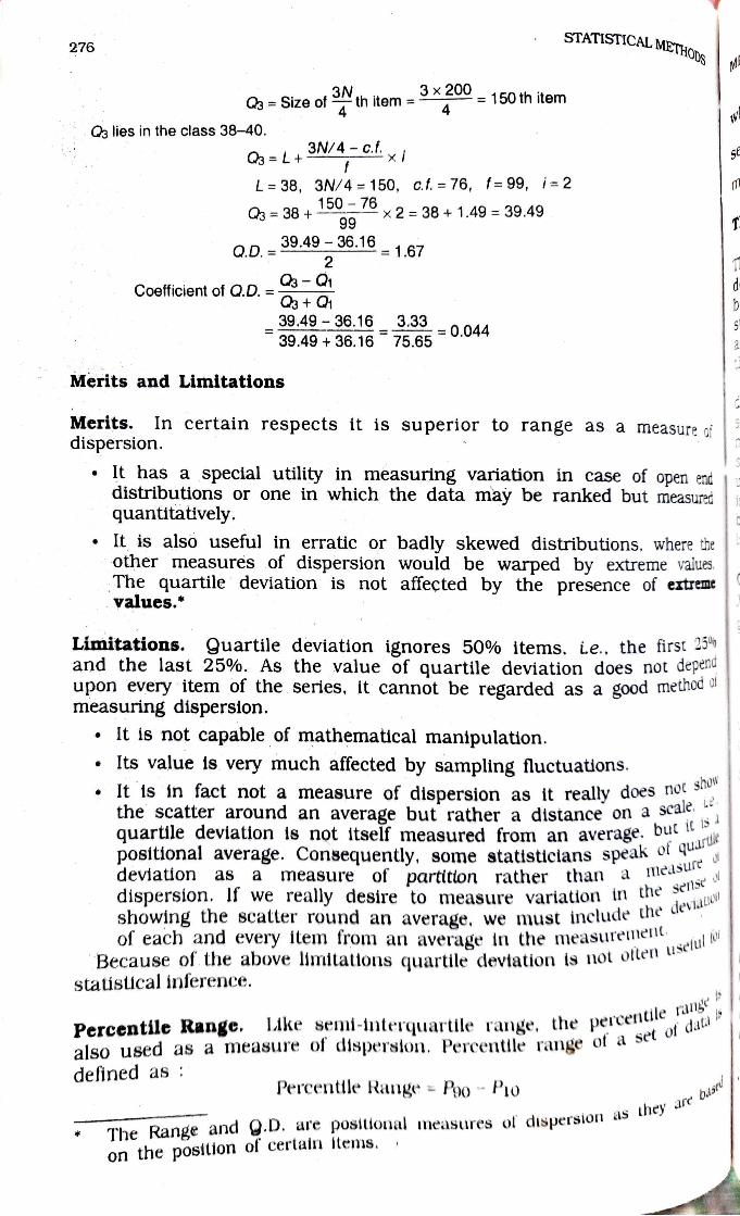
STATISTICAL METH ODS 276
Q3 Size ofth item =* = 150 th item 4
Q3 lies in the class 38-40.
3N/4-C.1:xi Q3 L+ L 38, 3N/4 150, c.f. = 76, f= 99, i=2
Q= 38+ 150-76x2 = 38 + 1.49 39.49 99
39.49 36.16 Q.D. = = 1.67 2
Coefficient of Q.D. = B + Q
39.49-36.163.35 - 0.044 39.49 +36.16 75.650.044
=
Merits and Limitations
Merits. In certain respects it is superior to range as a measure of dispersion. It has a special utility in measuring variation in case of open end
distributions or one in which the data may be ranked but measured quantitatively. It is also useful in erratic or badly skewed distributions. where the other measures of dispersion would be warped by extreme values The quartile deviation is not affected by the presence of ertreme values.
Limitations. Quartile deviation ignores 50% items. Le.. the first 2 and the last 25%. As the value of quartile deviation does not depend upon every item of the series, it cannot be regarded as a good methoc a
measuring dispersion. .It is not capable of mathematical manipulation.
Its value is very much affected by sampling fluctuations. Show
It is in fact not a measure of dispersion as it really does not the scatter around an average but rather a distance on a scai quartile deviation is not itself measured from an average. budke positional average. Consequently, some statisticians speak O e deviation as a measure of dispersion. If we really desire to measure variation in tnei
showing the scatter round an average, we must include ne of each and every item from an average in the measurenet selul
Because of the above limitations quartile devtation is not otet
statistical inference.
partitlon rather than a measur
devia
Percentile Range. LAke semi-interquartile range, the percentda
also used as a measure of disperslon. Percentile range ot a set
defined as
of
Percentle Range - Po0- P1o buse
The Range and 9.D. are positional measures of dispersion as ey
on the positlon f certaln items.
MEASUREs OF DISPERSION 277
where P90 and Pi0 are the 90th and 10th percentiles respectively. 1ne P semi-percentile range. Le.. | Pio can also be used, but is not com- 2
monly employed.
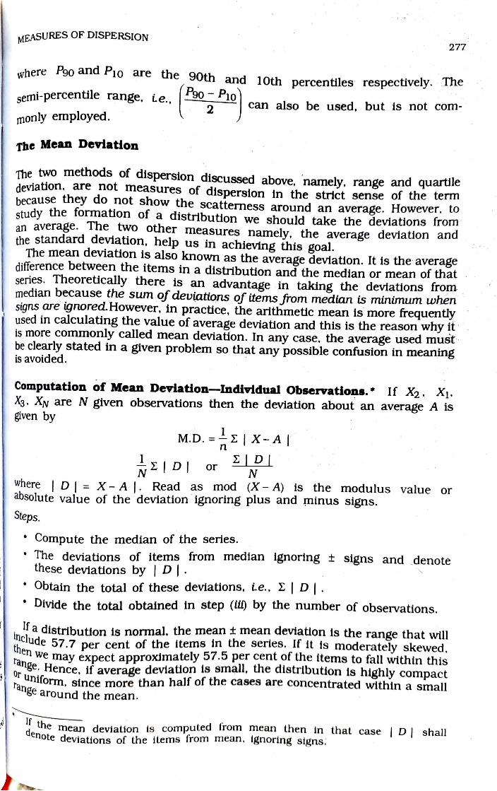
The Mean Deviation
The two methods of dispersion discussed above, namely, range and quarule deviation, are not measures of dispersion in the strict sense of the term because they do not show the scatterness around an average. However, to study the formation of a distribution we should take the deviations from an average. The two other measures namely, the average deviation and the standard deviation, help us in achieving this goal. The mean deviation is also known as the average deviation. It is the average difference between the items in a distribution and the median or mean of that series. Theoretically there is an advantage in taking the deviations from median because the sum of deviations of items from median is minimum when signs are ignored.However, in practice, the arithmetic mean is more frequently used in calculating the value of average deviation and this is the reason why it is more commonly called mean deviation. In any case, the average used must be clearly stated in a given problem so that any possible confusion in meaning is avoided.
Computation of Mean Deviation-Individual Observations. If X2. X1. X3. Xy are N given observations then the deviation about an average A is given by
M.D. X-A| DI EDI or
N where D = X- A |. Read as mod (X- A) is the modulus value or absolute value of the deviation ignoring plus and minus signs. Steps.
Compute the median of the series. The deviations of items from median 1gnoring t signs and denote these deviations by | D. Obtain the total of these deviations, ie., 2 |DI.
Divide the total obtained in step (it) by the number of observations. a distribution is normal. the mean t mean deviation is the range that will
Cude 57.7 per cent of the items in the serles. If it is moderately skewed. we may expect approximately 57.5 per cent of the items to fall within this
then ge. Hence, if average deviation 1s small, he distribution is highly compact
niform, since more than half of the cases are concentrated within a small or
Ange around the mean.
the mean deviation is computed Irom mean then in that case | DI shall note deviations of the items from mean, 1gnoring signs:
STATISTICAL METHODS 278
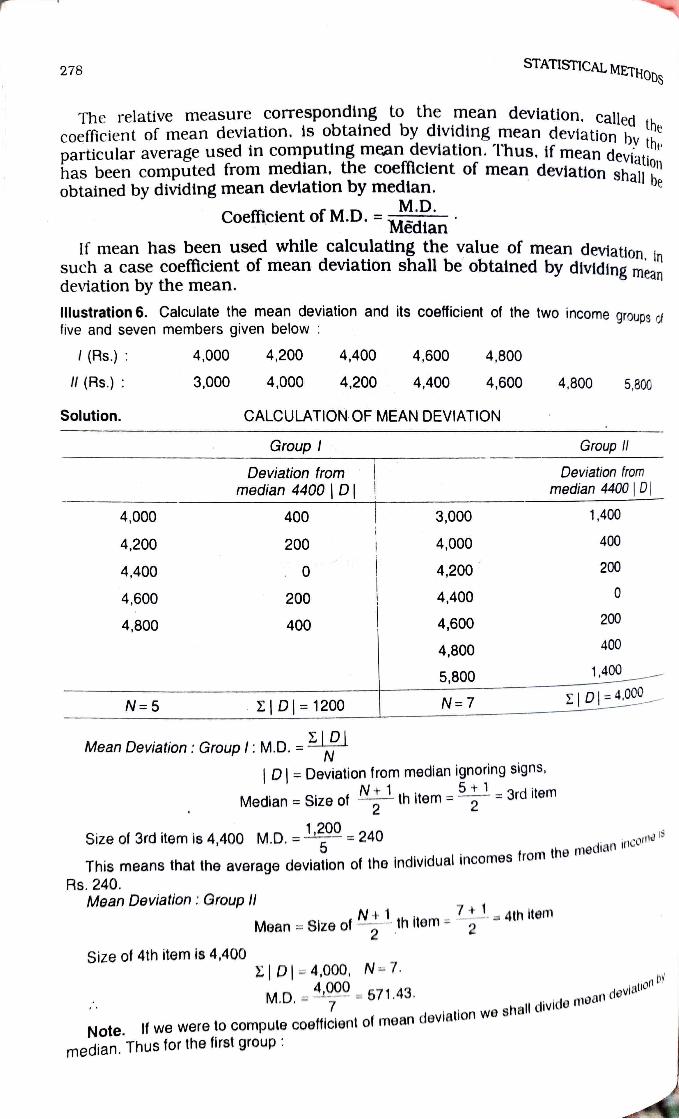
The relative measure corresponding to the mean deviation. called coefficient of mean deviation. is obtained by dividing mean deviation hy particular average used in computing mean deviation. Thus, if mean viation has been computed from median. the coefficient of mean deviation shal obtained by dividing mean deviation by median.
nall be
M.D. Coefficient of M.D. Median If mean has been used while calculating the value of mean deviation. in
such a case coefticient of mean deviation shall be obtained by dividing mean deviation by the mean.
llustration 6. Calculate the mean deviation and its coefficient of the two incorne grouos of five and seven members given below
(Rs.): 4,000 4,200 4,400 4,600 4,800
II (Rs.) 3,000 4,000 ,200 4,400 4,600 4,800 5,800
Solution. CALCULATION OF MEAN DEVIATION
Group Group Deviation from Deviation from
median 4400 | D| median 4400 | D|
4,000 400 3,000 1,400
4,200 200 4,000 400
4,400 4,200 200
600 200 4,400 0
,800 400 4,600 200
400 4,800
5,800 1,400
N=7 E|D= 4,000
5 2|D = 1200
Mean Deviation: Group I: M.D. = N
D= Deviation from median ignoring signs,
N+ 5 Median Size of th item = = 3rd item
2 2
Size of 3rd item is 4,400 M.D. = 1,200 240 5
This means that the average deviation of the individual incomes from the meua
Rs. 240.
Mean Deviation: Group Mean Size of th item 4th item
2 2
Size of 4th item is 4,400 2|D|= 4,000, N= 7.
4,000 M.D. 571.43.
7
10an devialion Dy
Note. If we were to compute coefficient of mean deviation we shall vi
median. Thus for the first group
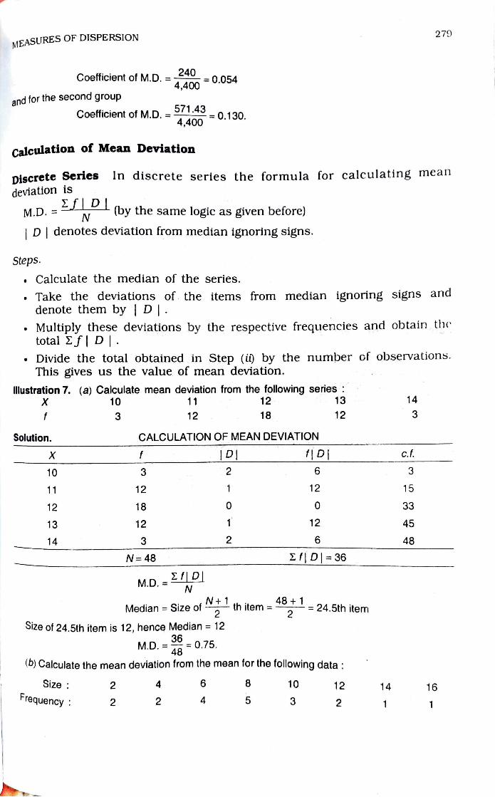
279 MEASURES OF DISPERSION
240Coefficient of M.D. = = 0.054 4,400
and for the second group
Coefficient of M.D. = 4_ 0.130. 4,400
Calculation of Mean Deviation
Discrete Series In discrete series the formula for calculating mean
deviation is
M.D. = I DI. N
(by the same logic as given before) D | denotes deviation from median ignoring signs.
Steps. Calculate the median of the seriesS. Take the deviations of. the items from median ignoring signs and
denote them by | D|.
.Multiply these deviations by the respective frequencies and obtain the
total 2f| DI. Divide the total obtained in Step (i) by the number of observations.
This gives us the value of mean deviation.
lustration 7. (a) Calculate mean deviation from the following series 11 13 14 12 X 10
3 18 12 3 12
CALCULATION OF MEAN DEVIATION Solution.
c.f. D X
3 2 6 10 3
12 15 1 11 12
0 33 0 12 18
12 45 12 13
48 2 6 3 14
Ef| D= 36 N 48
M.D. = 2IDI N
Median Size of th item =24.5th item 2 2
SIZe of 24.5th item is 12, hence Median = 12
M.D. 0.75. 48
(6) Calculate the mean deviation from the mean for the following data
12 6 10 14 16 Size 2 4
Frequency 2 A 5 3 2 1 2
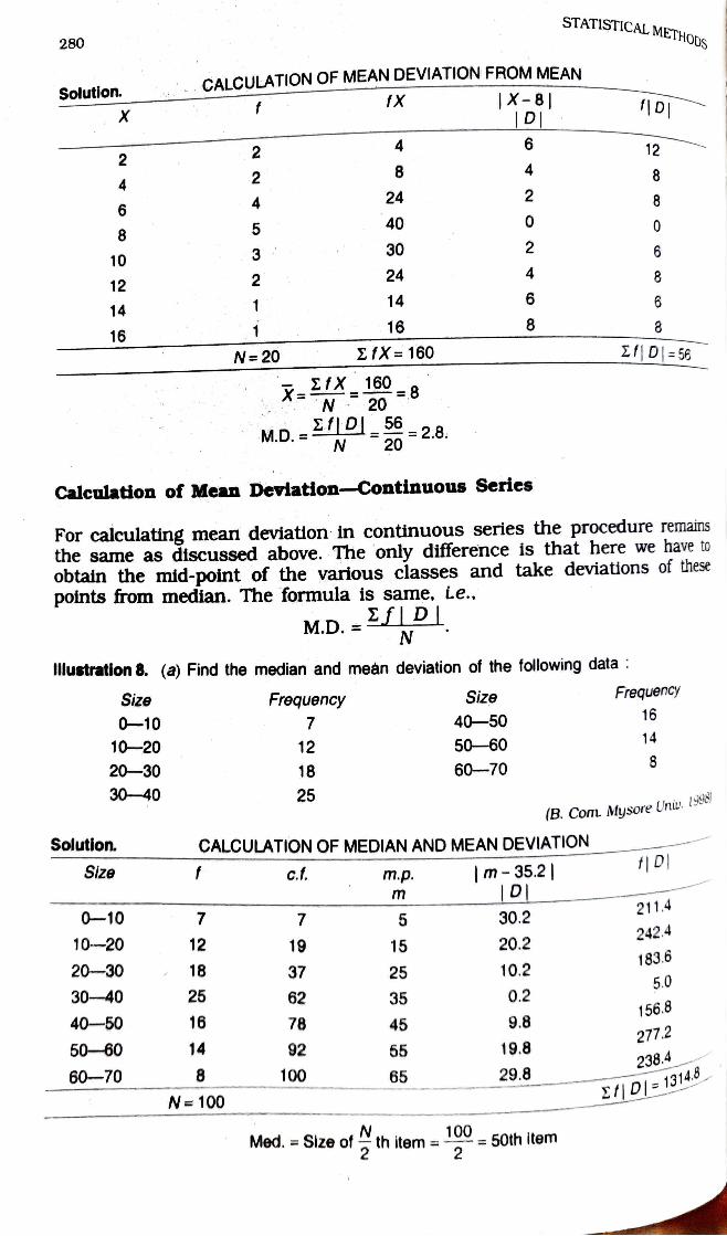
STATIS METH 280
CALCULATION OF MEAN DEVIATION FROM MEAN
X-8 D
Solution. f fX fD X
2 12 2
2 8 4
24 A 5 40
8 30 2
3 10 2 24 4
12 1 14
14 1 16
16
N 20 E fX= 160 ZfD=56
X- 20 IX 160 N
M.O.D1-=28. N 20
Calculation of Mean Deviation-Continuous Series
For calculating mean deviation in continuous series the procedure remains
the same as discussed above. The only difference is that here we have to
obtain the mid-point of the various classes and take deviations of these
points from median. The formula is same, ie., M.D.= 2I| DI
N
lustration 8. (a) Find the median and meân deviation of the following data
Size Frequency Size Frequency
16 0-10 7 40-50
14 10-20 12 50-60
8 20-30 18 60-70
30-40 25 (B. Com. Mysore Unu.
1998
Solution. CALCULATION OF MEDIAN AND MEAN DEVIATION f| D m-35.2
DI Size c.f. m.p.
m 211.4
0-10 7 7 30.2 242.4
10-20 12 19 15 20.2 183.6
20-30 18 37 25 10.2 5.0
30-40 25 62 35 0.2 156.8
40-50 16 78 45 9.8 277.2
50-60 14 92 55 19.8 238.4
60-70 8 100 65 29.8
N 100 E|D = 1314.8
Med. Size ofth item - 50th item
281 MEASURES OF DISPERSION
Median lies in the class 30-40
Med. =L+w2 xi
L30, N/2 -50, c.f. = 37, f= 25, i= 10
20503/ 10 = 30+5.2 35.2 25
M.D DI.1814.8. 13.148 100 N
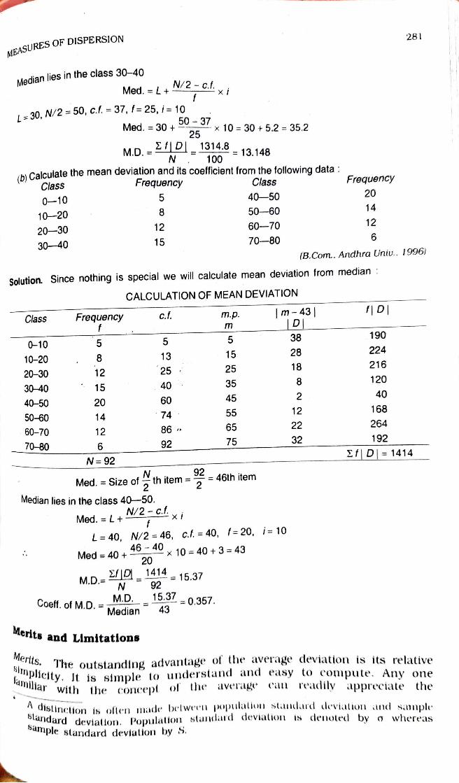
(h Calculate the mean deviation and its coefficient from the following data:
Class Frequency Class FrequencCy
5 40-50 20 0-10
8 50-60 14 10-20
12 60-70 12 20-30
6 15 70-80
30-40 (B.Com.. Andhra Univ.. 1996
Solution. Since nothing is special we will calculate mean deviation from median
CALCULATION OF MEAN DEVIATION
f DI m-43 DL Class Frequency c.f. m.p.
m 38 190
0-10 5 5
15 28 224 10-20 8 13
25 25 18 21620-30 12
40 35 8 12030-4 15
45 2 40 40-50 20 60
55 12 168 50-60 14 74
65 22 264 60-70 12 86
192 Ef| D= 1414
92 75 32 70-80 N= 92
Med. Size ofth item =46th item
Median lies in the class 40-50
Med. = L+ 2 i
f L= 40, N/2 = 46, c.f. = 40, f= 20, i= 10
Med 40+ 46-40x 10 = 40+ 3 = 43 20
M.D. D 1414 15.37 92 15.37 0,357.
N
M.D Coeff. of M.D. Median 43
Merits and Limitations
sS, The outstanding advantage of the average deviation is its relative Mert
am y. It is simple to understand and easy to conipute. Any one
"dr with the concept ol the averag Can readily appreciate the
stinction is often made betwer populilion stindard deviation and sannple
ndard deviation. Population slandrd devialioN 1s denoted by o whereas
anple standard deviallon Dy
MEASURES OF DISPERSION 283
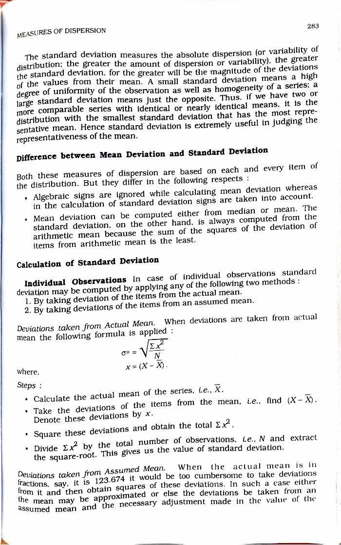
The standard deviation measures the absolute dispersion (or variability or
distribution; the greater the amount of dispersion or variability). the greater
the standard deviation, for the greater wil1 be the magnitude of the deviations
of the values from their mean. A small standard deviation means a high
degree of uniformity of the observation as well as homogeneity of a Series; a
large standard deviation means just the opposite. Thus. if we have two or
more comparable series with identical or nearly identical means, it is the
distribution with the smallest standard deviation that has the most repre
sentative mean. Hence standard deviation is extremely useful in judging the
representativeness of the mean.
Difference between Mean Deviation and Standard Deviation
Both these measures of dispersion are based on each and every item of
the distribution. But they differ in the following respects
Algebraic signs are ignored while calculating mean deviation whereas
in the calculation of standard deviation signs are taken into account.
Mean deviation can be computed either from median or mean. The
standard deviation, on the other hand. is always computed fromn the
arithmetic mean because the sum of the squares of the deviation of
items from arithmetic mean is the least.
Calculation of Standard Deviation
Individual Observations In case of individual observations standard
deviation may be computed by applying any of the following two methods
1. By taking deviation of the items from the actual mnean.
2. By taking deviations of the items from an assumed mean.
Deviations taken from Actual Mean. When deviations are taken from actual
mean the following formula is applied:
-V N
where. x= (X - X).
Steps Calculate the actual mean of the series. ie., X.
Take the deviations of the items from the mean, ie.. find (X- )
Denote these deviations by x.
Square these deviations and obtain the total Xx.
Divide Exby the total number of observations, ie., N and extract
the square-root. This gives us the value of standard deviation.
eviations taken from Assumed Mean.
Iractions, sav, it is 123.674 it woula be too cumbersome to take deviations
Irom it and then obtain squares of these deviations. In such a case either
he mean may be apprOximated or else the deviations be taken from an
assumed mean and the necessary adjustment made in the value of the
When the actual mean is in
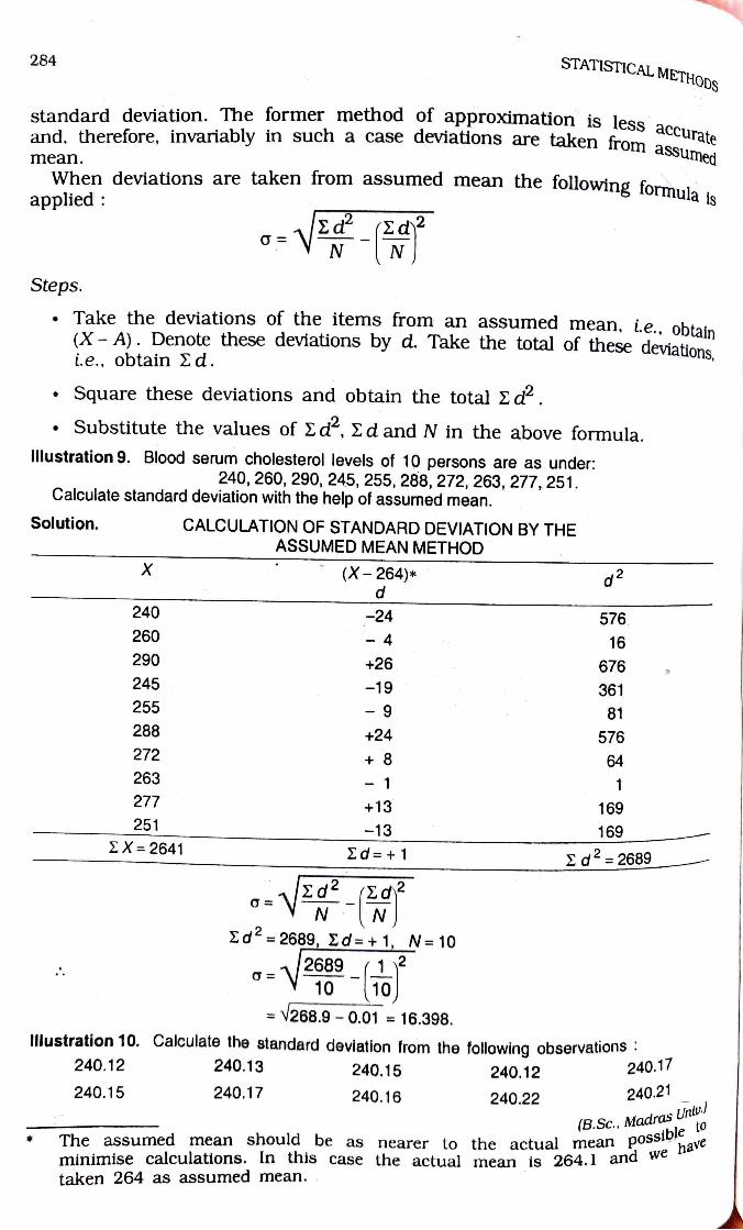
284 STATISTICAL METHODS standard deviation. The former method of approximation is less and. therefore, invariably in such a case deviations are taken from acurate accura from assumed mean.
When deviations are taken from assumed mean the following formila. applied: is
- 2d2
Steps. . Take the deviations of the items from an assumed mean, i.e., obtain (X A). Denote these deviations by d. Take the total of these deviations ie., obtain 2d.
Square these deviations and obtain the total 2 d2.
Substitute the values of 2d, 2d and N in the above formula.
Illustration 9. Blood serum cholesterol levels of 10 persons are as under:
240, 260, 290, 245, 255, 288, 272, 263, 277,251. Calculate standard deviation with the help of assurmed mean.
Solution. CALCULATION OF STANDARD DEVIATION BY THE ASSUMED MEAN METHOD
X (X-264)*
240 -24 576 260 4 16 290 +26 676 245 -19 361 255 9 81 288 +24 576 272 8 64 263 1 277 +13 169
251 2X= 2641
-13 169
d=+1 d 2689
N N
2d 2689, 2d=+ 1, N= 10 1/2689
10 = V268.9- 0.01 16.398.
Illustration 10. Calculate the slandard deviation from the following observations
240.12 240.13 240.15 240.12 240.17
240.15 240.17 240.16 240.22 240.21
The assumed mean should be as nearer to the actual mean
(B.Sc., Madras
poSSnve Univ e to
minimise calculations. In this case the actual mean is 264.1 and w taken 264 as assumed mean.
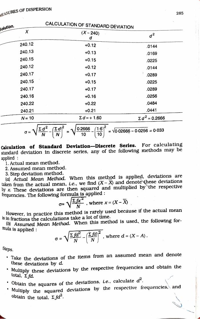
285 MEASUR OF DISPERSION
CALCULATION OF STANDARD DEVIATIONN solution.
X (X-240) d
2
240.12 +0.12 .0144 240.13 +0.13 0169
240.15 +0.15 0225 240.12 +0.12 0144
240.17 +0.17 0289
240.15 +0.15 0225
240.17 +0.17 0289
240.16 +0.16 0256
240.22 +0.22 .0484
240.21 +0.21 .0441
N= 10 Ed=+ 1.60 Zd=0.2666
V2558 =o02666-0-0256 = 0-033
Calculation of Standard Deviation--Discrete Series. For calculating
standard deviation in discrete series, any of the following methods may be
applied 1. Actual mean method. 2. Assumed mean method.
3. Step deviation method.
a Actual Mean Method. When this method is applied, deviations are
taken from the actual mean, ie., we find (X- X) and denote these deviationsS
by x. These deviations are then squared and multiplied by the respective
irequencies. The following formula is applied
- . where x= (X-X) N
However, in practice this method is rarely used because if the actual mean
in fractions the calculations take a lot of time.
bAssumed Mean Method. When this method is used. the following for-
mula is applied: where d = (X- A).
N
Steps. Take the deviations of the items from an assumed mean and denote
these deviations by d
Multiply these deviations by the respective frequencies and obtain the
total, E fd
Obtain the squares of the deviations, Le.. calculate ds.
Iultiply the squared deviations by the respective frequencies,\ and
obtain the total. fd".
STATISTICAL METHODOs 286
.Substitute the values in the above formula.
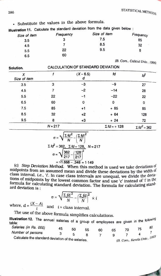
Illustration 11. Calculate the standard deviation from the data given below:
Frequency Size of item Frequency Size of item 7.5 85 3 3.5
7 8.5 32 4.5 22 9.5 8 5.5 60 6.5
(B. Com.. Calicut Untv.. 1996) CALCULATION OF STANDARD DEVIATION Solution.
f (X-6.5) fd X Size of item
3 -9 27 3.5
14 28 4.5
1 -22 22 5.5 22
60 0 0 6.5
85 85 7.5 85
32 +2 64 128 8.5
8 +3 +24 72 9.5
N=217 2fd=+128 fd=362
-V Efd2 (E fo N N
f 362, 2fd 128, N=217
362 (128 217 217 = V1.668-348 1.149
(c) Step Deviation Method. When this method is used we take deviations o midpoints from an assumed mean and divide these deviations by the widtn class interval, i.e., 'T. In case class intervals are unequal, we divide theu tions of midpoints by the lowest common factor and use 'c' instead ot t formula for calculating standard deviation. The formula for calculating sta ard deviation is
xi N
where, d = and i= class interval. The use of the above formula simplifies calculations.
llustration 12. The annual salaries of a group of employees are given in the folow table Salaries (in Rs. 000) Number of persons
Calculate the standard deviation of the salaries.
80 45 50 55 60 65 70 75 7
4 3 5 8 7 9 7
(B. Com. Kerela Univ., 195
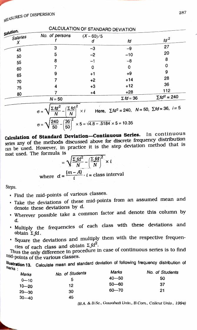
287 MEASURES OF DISPERSION
CALCULATION OF STANDARD DEVIATION Solution.
Salaries
X
No. of persons (X-60)/5 f fd fd
27 45 3 3 -9
5 2 -10 20 50
8 -1 -8 8 55
60 7 0
9 +1 +9 9 65
28 70 +2 +14
4 +3 12 36 75
112 +28 fd 36
80 +4
N= 50 Efd2 240
g= V2/d(2td V - xi Here, Efd2 = 240, N= 50, Efd= 36, i= 5
N
o-5050 240 36 x5 V4.8 5184 x 5 10.35
Calculation of Standard Deviation-Continuous Series. In continuous
series any of the methods discussed above for discrete frequency distribution
can be used. However, in practice it is the step deviation method that is
most used. The formula is
xi N N
where d = . i= class interval
Steps. Find the mid-points of various classes.
Take the deviations of these mid-points from an assumed mean and
denote these deviations by d.
Wherever possible take a common factor and denote this column by
d.
Multiply the frequencies of each clasS with these deviations and
obtain 2d.
Square the deviations and multüply them with the respective frequen-
cies of each class and obtain 2fd".
.nus the only difference in procedure in case of continuous series is to find
d-points of the various classes.
Ustration13. Calculate mean and standard deviatlon of following frequency distribution of
marks Marks No. of Students Marks No. of Students
0-10 5 40-50 50
10-20 12 50-60 37
20-30 30 60-70 21
30-40 45 (B.A. &B.Sc., Guwahatt Untv., B.Com., Calicut Univ. 1994)
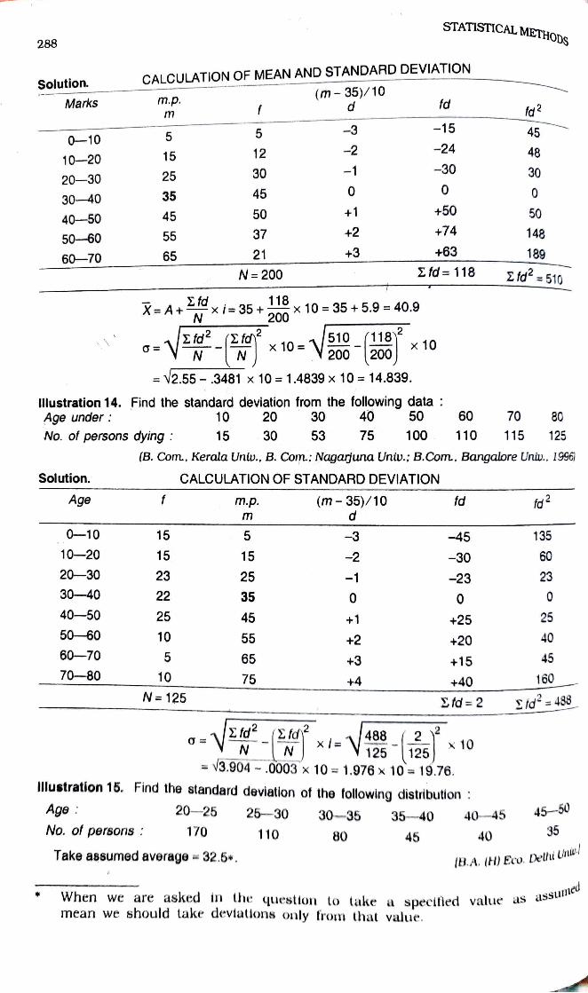
STATISTICAL METHODs 288
Solution. CALCULATION OF MEAN AND STANDARD DEVIATION
(m-35)/10 d Marks m.p. fd
m fd2
5 -3 -15 45 0-10 5
12 -24 48 10-20 15
25 30 -30 30 20-30
30-40 35 45
45 50 +1 +50 50 40-50
55 37 +2 +74 148 50-60
60-70 65 21 +3 +63 189
N= 200 Z fd 118 fd 510 2 fd =A+xi= 35+x 10 35+5.9 = 40.9
200 N
o- 2 fd ( fd x 10 510 (118 10
V 200 200
= V2.55 3481 x 10 1.4839x 10 = 14.839.
Wlustration 14. Find the standard deviation from the following data : 10 20 30 40 50 60 70 80 Age under
No. of persons dying9 15 30 53 75 100 110 115 125
(B. Com.. Kerala Unw., B. Com.: Nagarjuna Univ.; B.Com, Bangalore Unw., I1996)
Solution. CALCULATIiON OF STANDARD DEVIATION
Age m.p. (m-35)/10 fd fd m
0-10 15 -45 135
10-20 15 15 -2 -30 60
20-30 23 25 -23 23 30-40 22 35 0
40-50 25 45 +1 +25 25
50-60 10 55 +2 +20 40
60-70 5 65 +3 +15 45 70-80 10 75 +4 +40 160
N=125 fd 2 Id 488
a-2- xi-V1510 = v3.904- .0003x 10 1.976 x 10 19.76.
llustration 15. Find the standard deviation of the following distribution :
Age 20-25 25-30 30-35 35-40 40-45 45-50
No. of persons 170 110 80 45 40 35
Take assumed average = 32.5*. BA. (H) Eco. Delhi Unit
When we are asked in the question to take a specitied value as a* mean we should take deviatlons only from that value.
alue as assumed
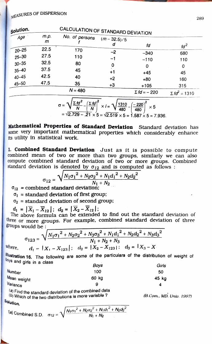
MEASURES OF DISPERSION
289
CALCULATION OF STANDARD DEVIATION Solution.
m.p No. of persons (m- 32.5)/5 Age m f
d fd 20-25 22.5 170
-340 680 25-30 27.5 110
-110 110 30-35 32.5 80 0 35-40 37.5 45 +1 +45 45 40-45 42.5 40 +2 +80 160 45-50 47.5 35 +3 +105 315
N 480 2fd= - 220 ff 1310
a- x= 11310(-220 x5 480 480
= v2.729 21 x5 V2.519 x 5= 1.587 x 5 = 7.936.
Mathematical Properties of Standard Deviation Standard deviation has some very important nmathematical properties which considerably enhance its utility in statistical work.
1. Combined Standard Deviation Just as it is possible to compute combined mean of two or more than two groups, similarly we can als0 compute combined standard deviation of two or more groups. Combined standard deviation is denoted by d12 and is computed as follows
O2-VMo1+ No2 + Nd2+ Nad,? Ni + N2
O12 combined standard deviation; O standard deviation of first group; 2 standard deviation of second group:
d |X - X12: dh = | X2- X12l: The above formula can be extended to find out the standard deviation of
three or more groups. For example. combined standard deviation of three groups would be
09=VNo+ Nao2 + Ngogí+ Nd+ Nada + Ngd2 N1 + N2 + Na O123 V
where d = IX, - X123 dh = |X2- X123 d = X3 - X
lustration 16. The following are some of the particulars of the distribution of weight oft 0Oys and girls in a class
Boys Girls Number 100 50
Mean weight Variance
a the standard deviation of the combined data
60 kg 45 kg
4
wnich of the two distributions is more variable ?
Solution. (B.Com. MD. Unu. 1997)
Ta) Combined S.D. o12= V N101 N202+ Nidh+N2d2
Ni + N
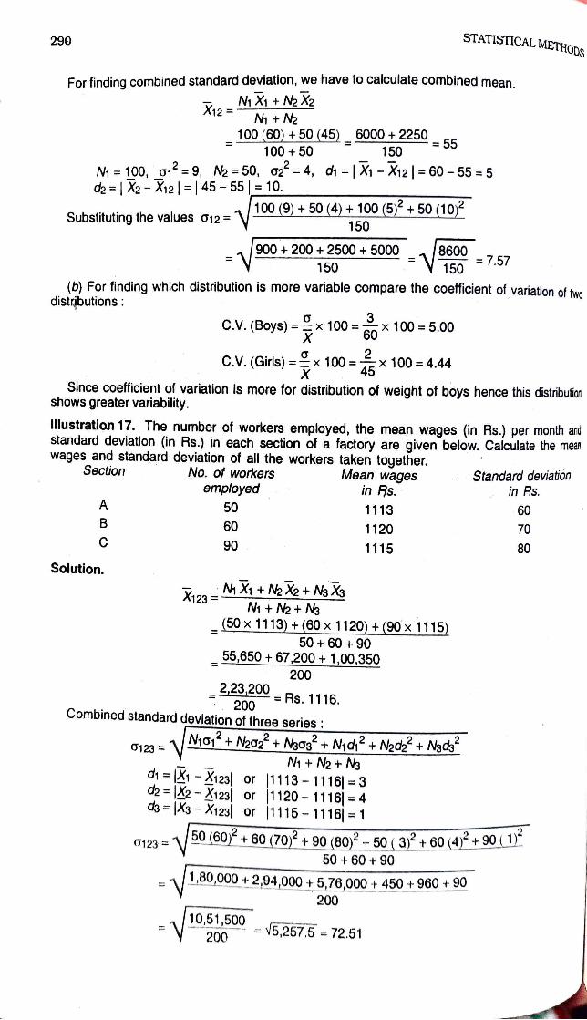
STATISTICAL METHODs 290
For finding combined standard deviation, we have to calculate combined mean.
X12 +2X2 N + N2
100 (60)+50 (45) 6000+2250cc = 100+50 150
N 100, o=9, N2 50, o2 = 4, dh = | Xi - X12|= 60- 55 5
d=| X2- X12| = |45-55|= 10.
100 (9)+50 (4)+ 100 (5) +50 (102 150
Substituting the values o12 V
86007.57 150 900+200 + 2500+ 5000
150 (b) For finding which distribution is more variable compare the coefficient of variation of w
distributions C.V. (Boys)= x 3 100 5.00
50
C.V.(Girls) x 100-x 100-4.44Since coefficient of variation is more for distribution of weight of boys hence this distribution
shows greater variability.
llustration 17. The number of workers employed, the mean wages (in Rs.) per month and standard deviation (in Rs.) in each section of a factory are given below. Calculate the mean wages and standard deviation of all the workers taken together.
Section No. of workers Standard deviation Mean wages in Rs. employedd in Rs.
50 1113 60 B 60 1120 70 C 90 1115 80
Solution.
NX +X2t NaXa Ni +N2+ Na
(50x 1113) + (60x 1120) + (90x 1115) 50+60+ 90
55,650+67,200+1,00,350 200
2,23,200 = Rs. 1116.
Combined standard deviation of three series 200
O123=1io" + Ng2+ Noas+ Nid+Nadh+ Ngcd M + Ne + Na
d = X1 -X1231 or |1113- 1116 =3
d2 X2-X123 or |1120- 1116 = 4 d Xg- X123| or |1115-1116 1
50 (60+60 (70) +90 (80)+ 50 ( 3) + 60 (4 + 90 (1) 2
0123=
50+60+ 90
1,80,000 +2,94,000 +5,76,000 + 450+960 + 90 F
200
10,51,500 N V5,257.5 72.51 200
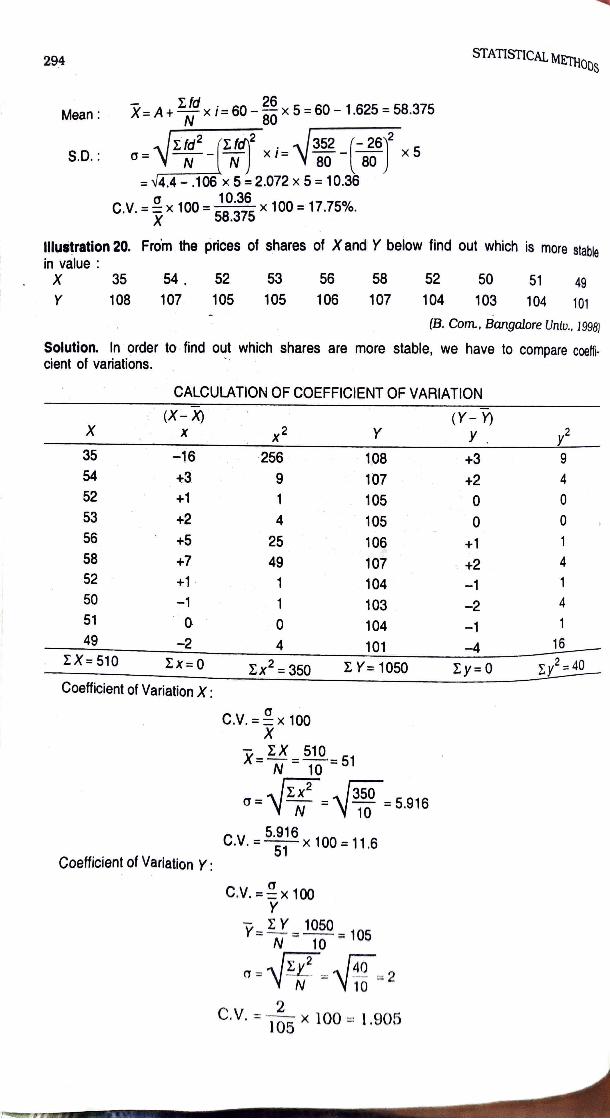
STATISTICAL METHOD 294
Mean: X=A+x i=60 x 5 60 1.625 58.375
G-dExi=V352-26x5 S.D. 80
C.V.x 100 58.375 x 100 17.75%.
= V4.4-.106 x 5 2.072 x 5 = 10.36
10.36
llustration 20. From the prices of shares of Xand Y below find out which is more stable
in value: X 35 54 52 53 56 58 52 50 51 49 Y 108 107 105 105 106 107 104 103 104 101
(B. Com., Bangalore Univ., 1998)
Solution. In order to find out which shares are more stable, we have to compare coetf cient of variations.
CALCULATION OF COEFFIIENT OF VARIATION (Y-Y (X-X)
X Y
35 -16 256 108 +3 54 +3 107 +2 4 52 +1 105 0 0 53 +2 105 0 56 +5 25 106 58 +7 49 107 52 +1 104 50 103 51 0 0 104 49 2 101 -4 16
ZX= 510 Ex= 0 2=350 EY= 1050 y 0 Ey40 Coefficient of Variation X:
C.V.x 100
2510 51 N 10 =51
N 350 5.916 10
C.V.= x 100 11.6 51
Coefficient of Variation Y:
C.V.x 100
Y-Y1050 1 105
- 140 N 10
V10 2
C.V. = x 100 = 1.905
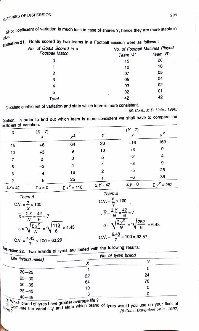
295 1ASURES OF DISPERSION
nt of variation is much less in case of shares Y, hence they are more stable in Since coefficient
value.
tlustras
etration 21. Goals scored by two teams in a Football session were as follows
No. of Goals Scored in a Football Match
No. of Football Matches Played Team B' Team 'A'
0 15 20
10 10
2 07 05
05 04
4 03 02
5 02 01
Total 42 42
Calculate coefficient of variation and state which team is more consistent.
(B. Com, M.D. Uniu., 1996)
Solution. In order to find out which team is more consistent we shall have to compare the
coeficient of variation.
(Y-7) X (X-7) Y y2 2
20 +13 169 15 +8 64
10 +3 9 10 +3
5 -2 4 0
4 -3 9 2
16 2 5 25
-6 36 -5 25
Y= 42 Ey=0 y252 X= 42 2x= 0 Ex 118
Team B Team A
C.V.x 100 C.V.x 100
X
. 7 a 2526.A48
427
E 118 -4.43g N
CV. x 100 92.57 C.V x 100 63.29 7
on 22. Two brands of tyres are tested with the following results: Mustra Life (in'000 miles) No. of tyres brand
20-25 22 24
25-30 64 76
30-35 10
35-40 3
40-45 mpare the variability and state which Drand of tyres would you use on your fleet of
Comp tyres have greater average life ?
(B.Com.. Bangalore Untv., 1997)
Scanned with FlashScan