
The Dopaminergic Midbrain Encodes the Expected Certainty about Desired Outcomes
Upload
khangminh22Category
view
0download
0
Expected Idiosyncratic Skewness
Brian BoyerBrigham Young University
Todd MittonBrigham Young University
Keith VorkinkBrigham Young University
We test the prediction of recent theories that stocks with high idiosyncratic skewness shouldhave low expected returns. Because lagged skewness alone does not adequately forecastskewness, we estimate a cross-sectional model of expected skewness that uses additionalpredictive variables. Consistent with recent theories, we find that expected idiosyncraticskewness and returns are negatively correlated. Specifically, the Fama-French alpha of alow-expected-skewness quintile exceeds the alpha of a high-expected-skewness quintile by1.00% per month. Furthermore, the coefficients on expected skewness in Fama-MacBethcross-sectional regressions are negative and significant. In addition, we find that expectedskewness helps explain the phenomenon that stocks with high idiosyncratic volatility havelow expected returns. (JEL D03, G11, G12)
Finance research has a long history of investigating the impact of return skew-ness on investor decision making. Arditti (1967) and Scott and Horvath (1980)show that under very general assumptions, investors demonstrate a preferencefor positive skewness in return distributions. Building on these results, Krausand Litzenberger (1976) and Harvey and Siddique (2000) show that an asset’scoskewness with the market portfolio should be priced in a representative agentframework. Because these studies are set in the context of fully diversified in-vestors, they imply that a stock’s idiosyncratic skewness should be irrelevant.However, others have noted that because diversification erodes skewness ex-posure, some investors may remain underdiversified in order to capture returnskewness, and thus idiosyncratic skewness may be relevant (see Simkowitz andBeedles 1978; Conine and Tamarkin 1981).
We appreciate the helpful comments of Andrew Ang, Nicholas Barberis, Antti Ilmanen, Grant McQueen,Jonathan Parker, Steven Thorley, Rossen Valkanov, Tuomo Vuolteenaho, and seminar participants at BrighamYoung University and the participants of the 2007 China International Conference in Finance. We acknowl-edge financial support from the Harold F. and Madelyn Ruth Silver Fund, Intel Corporation, and our Fordresearch fellowships. We thank Greg Adams for research support. Send correspondence to Brian Boyer, MarriottSchool of Management, 640 TNRB, Brigham Young University, Provo, UT 84602; telephone: 801-422-7641;fax: 801-422-0108. E-mail: [email protected].
C© The Author 2009. Published by Oxford University Press on behalf of The Society for Financial Studies.All rights reserved. For Permissions, please e-mail: [email protected]:10.1093/rfs/hhp041 Advance Access ublication June 3, 2009p
at Pennsylvania State University on February 21, 2016
http://rfs.oxfordjournals.org/D
ownloaded from
Recent theories—each starting from a different set of assumptions—concurthat idiosyncratic skewness can be a priced component of stock returns. Mittonand Vorkink (2007), in a model incorporating heterogeneous investor prefer-ence for skewness, predict lower expected returns for stocks with idiosyncraticskewness. Barberis and Huang (2007) show that when investors have cumu-lative prospect theory preferences, stocks with greater idiosyncratic skewnessmay have lower average returns. Brunnermeier and Parker (2005) and Brun-nermeier, Gollier, and Parker (2007) solve an endogenous-probabilities modelthat produces similar asset pricing implications for skewness.
In this paper, we empirically investigate the pricing implications of idiosyn-cratic skewness. Despite the theoretical basis for the pricing effects of skewnesspreference, empirically testing the relation between idiosyncratic skewnessand returns is not a straightforward exercise. The primary obstacle is thatex ante skewness is difficult to measure. As opposed to variances and covari-ances, idiosyncratic skewness is not stable over time (see Harvey and Siddique1999), so variables other than lagged skewness are required to effectively mea-sure expected skewness. We follow the approach of Chen, Hong, and Stein(2001) in using a number of firm-level variables to predict idiosyncratic skew-ness. We find that, although lagged skewness is an important predictor of futureskewness, other firm characteristics are also important predictors of idiosyn-cratic skewness, including idiosyncratic volatility, a measure that has recentlygenerated considerable interest in asset pricing. Other important predictive vari-ables in our model include momentum and turnover (see Hong and Stein 2003;Chen, Hong, and Stein 2001), firm size, and industry designation. Our predic-tive model produces distinct variation in expected skewness across stocks aswell as over time. The time-series variation in both realized and expected skew-ness appears to follow episodic behavior similar to the behavior of idiosyncraticvolatility (see Campbell et al. 2001; Brandt et al. 2008).
Using our model of expected skewness, we find a strong negative cross-sectional relation between expected idiosyncratic skewness and average re-turns. We sort firms into quintiles based on their level of expected skewness.We find that the average returns for the low-expected-skewness quintile exceedthe average returns of the high-expected-skewness quintile by 0.67% per month.After adjusting for risk, the differences in returns are even more pronounced.We find that the Fama-French (1993) alpha of the low-expected-skewness quin-tile exceeds the Fama-French alpha of the high-expected-skewness quintile by1.00% per month. We confirm the pricing effects of idiosyncratic skewness byestimating Fama-MacBeth (1973) regressions, and find that expected skewnesshelps explain the cross-sectional variation in returns. The effect of idiosyncraticskewness is statistically significant and is robust in a number of alternative spec-ifications. This finding is consistent with Zhang (2005), who finds a negativerelation between total skewness and average returns when estimating skewnessbased on the cross-sectional returns of a group of comparable stocks. We per-form additional tests to distinguish the separate effects of expected skewness
170
The Review of Financial Studies / v 23 n 1 2010
at Pennsylvania State University on February 21, 2016
http://rfs.oxfordjournals.org/D
ownloaded from
Expected Idiosyncratic Skewness
and idiosyncratic volatility, and find that each has significant explanatory powerfor expected returns independent of the other.
We also explore whether the time-series variation in expected skewness isrelated to the time-series variation in the expected skewness risk premium.We find that the periods in which the cross-sectional estimate of the expectedskewness premium is most significant and negative correspond to periods inwhich the level and dispersion of expected skewness is high and in which ourmodel of predicted skewness fits the data well (high R2). One interpretationof these relations is that the pricing of skewness is strongest in those periodsin which there are greater opportunities for skewness-preferring investors toexpress their preference for securities with upside potential.
Having documented the pricing implications of idiosyncratic skewness, weturn to the question of whether skewness can help explain the phenomenonthat stocks with high idiosyncratic volatility have low expected returns. Thenegative relation between idiosyncratic volatility and future returns, whichwe refer to as the “iv puzzle,” is documented in the U.S. data in Ang et al.(2006), and is shown to be present in international markets in Ang et al.(2008). The iv puzzle has generated substantial interest among researchers.1
A negative relation between idiosyncratic volatility and expected returns ispuzzling because standard theory does not account for such a relation. Onone hand, if investors fully diversify, then idiosyncratic volatility should notbe priced at all. On the other hand, if investors do not fully diversify, thenidiosyncratic volatility should be positively related to the expected returns (seeMerton 1987; Malkiel and Xu 2006). However, our finding that idiosyncraticvolatility is a strong predictor of idiosyncratic skewness suggests a novel reasonwhy investors may be attracted to stocks with high idiosyncratic volatility.Investors may accept lower average returns on stocks with high idiosyncraticvolatility, not because they seek higher volatility, but because they have apreference for stocks with lottery-like return properties.
We conduct tests to assess the impact of skewness preference on the iv puzzle.Using our model of predicted skewness, we study the relation between idiosyn-cratic volatility and expected returns after controlling for forecasted skew-ness. We construct portfolios with wide dispersion in idiosyncratic volatilitybut low dispersion in expected idiosyncratic skewness using the conditional-sorting methodology used by Ang et al. (2008) and others. After controllingfor expected idiosyncratic skewness, the relation between idiosyncratic volatil-ity and returns is weaker. In particular, we find that the difference betweenthe average returns of the high-idiosyncratic-volatility portfolio and the aver-age returns of the low-idiosyncratic-volatility portfolio is much smaller andinsignificant. Moreover, the difference between the Fama-French alphas ofthe high-idiosyncratic-volatility portfolio and the low-idiosyncratic-volatility
1 See, for example, Bali and Cakici (2008); Huang et al. (2006); Boehme et al. (2005); Duan, Hu, and McLean(2006); Jiang, Xu, and Yao (2008); Fu (2005); and Kapadia (2006).
171
at Pennsylvania State University on February 21, 2016
http://rfs.oxfordjournals.org/D
ownloaded from

portfolio is reduced from 1.30% per month to 0.48% per month. Skewness pref-erence appears to be important in explaining the low average returns of stockswith high idiosyncratic volatility. We further attempt to disentangle the separateeffects of expected skewness and idiosyncratic volatility and find that, whileboth characteristics have independent explanatory power for expected returns,there is also some overlapping explanatory power that could be attributed toeither characteristic. Although it would be difficult to determine empirically towhat this overlapping portion should be properly attributed, we argue that thenegative relation between expected idiosyncratic skewness and average returnshas stronger theoretical support.
The rest of the paper is organized as follows. Section 1 presents the motivationfor our empirical tests, focusing on the theoretical connections for skewnesspreference and expected returns. Section 2 reports the results of our estimationof a skewness prediction model. Section 3 investigates the pricing implicationsof idiosyncratic skewness. Section 4 further distinguishes between the effects ofidiosyncratic skewness and volatility and explores whether skewness preferenceexplains the negative relation between idiosyncratic volatility and expectedreturns. Section 5 offers concluding remarks.
1. Motivation
To motivate our empirical investigation, we draw on a number of differentpapers in the asset pricing literature. Speculative behavior on the part of in-vestors, particularly individual investors, has motivated multiple theoreticalmodels attempting to understand the impact of this type of behavior on assetprices. For example, Mitton and Vorkink (2007) develop a model of hetero-geneous preference for skewness. Essential to their model is the assumptionthat some investors (“lotto investors”) have a preference for positive skewnesswhile others (“traditional investors”) are mean-variance optimizers seeking tomaximize the Sharpe ratio of their portfolios. Stock returns have exogenoussecond and third moments. Lotto investors place a higher value on stocks withpositive idiosyncratic skewness and choose to hold underdiversified portfoliosto increase their exposure to positive skewness. Markets clear at prices suchthat stocks with high idiosyncratic skewness have negative alphas relative tothe value-weighted market portfolio. In equilibrium, both lotto investors andtraditional investors choose portfolio weights such that the marginal cost ofholding additional shares is equal to the marginal benefit. Thus, in Mittonand Vorkink (2007), investors hold underdiversified portfolios in equilibrium,and total skewness (including idiosyncratic skewness) is priced. Empirically,Mitton and Vorkink (2007) find their model’s predictions help to explain portfo-lio behavior in a dataset consisting of household accounts from a large discountbrokerage.
Alternatively, Barberis and Huang (2007) develop a model with investorshaving cumulative prospect theory preferences in which, similar to Mitton and
172
The Review of Financial Studies / v 23 n 1 2010
at Pennsylvania State University on February 21, 2016
http://rfs.oxfordjournals.org/D
ownloaded from
Expected Idiosyncratic Skewness
Vorkink (2007), holdings are heterogeneous across agents in equilibrium. Incontrast to Mitton and Vorkink (2007), agents have identical preferences, butthe equilibrium obtained is one where some agents hold highly underdiversifiedportfolios. Cumulative prospect utility theory suggests that, through a weightingfunction, agents overweight the probabilities in the extremes. Barberis andHuang (2007) show that when securities have return distributions that areskewed, the equilibria that result from agents having cumulative prospect theorypreferences include the pricing of the idiosyncratic skewness of a stock’s return.
In addition, Brunnermeier and Parker (2005) develop a structural asset pric-ing model in which agents optimize over beliefs of outcomes, as opposed totaking probabilities as primitives. Agents derive felicity, analogous to utility,from increasing their beliefs about probabilities above the “true” levels on highpositive payoff states as long as the costs of doing so do not offset this additionalutility. This optimizing behavior of agents leads to, among other predictions, astrong preference for securities with skewed distributions (see their PropositionII). Brunnermeier, Gollier, and Parker (2007) show that optimal expectationsreduce the average returns of skewed assets in general equilibrium. These the-oretical predictions of a negative relation between idiosyncratic skewness andexpected returns motivate our empirical investigation.2
Since forecasting skewness is essentially an exercise in forecasting small-probability events, this exercise is inherently difficult. Although asset pricingtests often use lagged predictors of second moments (beta and volatility) asproxies for expected levels based on the widely supported assumption thatsecond moments are persistent, this approach appears problematic for thirdmoments. For example, Harvey and Siddique (1999) estimate models of time-varying skewness and find that a lagged measure of skewness is, at best, a weakpredictor of skewness (the autoregressive parameter for monthly skewness isabout −0.4). The challenge is thus to find an appropriate way to measureexpected skewness.
Zhang (2005) proposes one approach to measure expected skewness in whichhe estimates individual stock skewness based on the recent past cross-sectionalskewness of stocks in a “peer group” (such as industry). Chen, Hong, andStein (2001) introduce another approach in which, motivated by the model ofHong and Stein (2003), they analyze predictors of firm skewness by estimatingpredictive regressions across a wide cross-section of stocks.3 Our econometricapproach builds upon Chen, Hong, and Stein (2001) by constructing measures
2 The theoretical models motivating our empirical analysis predict that total (not just idiosyncratic) skewnessmatters to investors. We use idiosyncratic skewness as our measure of interest for two reasons. First, by focusingon the idiosyncratic component of skewness, we highlight the distinguishing features of the theoretical modelsmotivating our empirical analysis—that investors may hold portfolios that are not well diversified and as a resultcare about security-specific features of the return distribution (i.e., idiosyncratic volatility and skewness). Second,by focusing on idiosyncratic skewness, we distinguish our empirical results from existing papers that investigatethe pricing of skewness (e.g., Kraus and Litzenberger 1976; Harvey and Siddique 2000). As a robustness check,we conduct asset pricing tests using total return skewness and find similar results in both statistical and economicmagnitude to idiosyncratic skewness.
3 Chen, Hong, and Stein (2001) actually estimate panel models of negative skewness motivated by the crash modelof Hong and Stein (2003).
173
at Pennsylvania State University on February 21, 2016
http://rfs.oxfordjournals.org/D
ownloaded from
of expected skewness each month for a given firm using past returns and tradingvolume as well as firm characteristics. Cross-sectional regression models arethen used to predict skewness. Our approach also draws upon the work ofHarvey and Siddique (1999) on the time-series properties of return skewnessin that our model includes lagged skewness as a predictive variable.
We find, among other results, that lagged idiosyncratic volatility is a strongpositive predictor of firm skewness (see also Chen, Hong, and Stein 2001;Kapadia 2006). Idiosyncratic volatility could be a strong predictor of skewnessfor at least three reasons. First, idiosyncratic volatility is positively related tocorporate growth options (see Cao, Simin, and Zhao 2006; Barinov 2006),and the presence of growth options implies greater skewness in returns (e.g.,Andres-Alonso, Azofra-Palenzuela, and de la Fuente-Herrero 2006). Second,higher idiosyncratic volatility may be related to technological revolutions (seePastor and Veronesi 2007), and these revolutions may lead to industry shakeouts(Jovanovic and MacDonald 1994) which in turn imply greater skewness inreturns as a few winners emerge and other firms fail. Third, simply from amechanical standpoint, limited liability of equity implies that greater volatilityleads to greater skewness (e.g., Conine and Tamarkin 1981). In the next section,we use idiosyncratic volatility, as well as other variables suggested by theliterature, to estimate a model of expected skewness.
2. A Skewness Prediction Model
We develop a model of expected skewness that incorporates past returns andtrading volume as well as known firm characteristics. Let the investment horizonover which investors are hoping to experience an extreme positive outcome beT months, let S(t) denote the set of trading days from the first day of montht − T + 1 through the end of month t , and let N (t) denote the number ofdays in this set.4 Let εi,d be the regression residual using the Fama and French(1993) three-factor model on day d for firm i , where the regression coefficientsthat define this residual are estimated using daily data for days in S(t). Inaddition, let ivi,t and isi,t denote historical estimates of idiosyncratic volatilityand skewness (respectively) for firm i using daily data for all days in S(t), andlet k be the number of factors in the regression. We can then define ivi,t andisi,t as
ivi,t =(
1
N (t)
∑d∈S(t)
ε2i,d
)1/2
, (1)
isi,t = 1
N (t)
∑d∈S(t) ε
3i,d
iv3i,t
. (2)
4 In our construction of skewness estimates, N (t) is the number of days in the set minus a degrees of freedomadjustment of one for volatility and two for skewness. Alternative choices for the adjustment to N (t) cause verylittle difference in the pricing results.
174
The Review of Financial Studies / v 23 n 1 2010
at Pennsylvania State University on February 21, 2016
http://rfs.oxfordjournals.org/D
ownloaded from

Expected Idiosyncratic Skewness
−2
0
2
4
6
1930
1935
1940
1945
1950
1955
1960
1965
1970
1975
1980
1985
1990
1995
2000
2005
Fir
m S
kew
ness
10 (90) Percentiles
25 (75) Percentiles
Median
Figure 1Cross-sectional distribution of firm-level skewnessThe 10th, 25th, 50th, 75th, and 90th percentiles of the monthly cross-sectional distribution of idiosyncratic firmskewness, isi,t , for all NYSE-listed companies from January 1930 through December 2005.
Figure 1 plots the cross-sectional distribution of isi,t for t equal to December1929 through December 2005, and T = 60 months, using stocks that trade onthe NYSE. In particular, we plot the 10th, 25th, 50th, 75th, and 90th percentilesof isi,t each month. All of the reported percentiles show time variation, but the90th percentile exhibits the greatest variation, and has particularly large move-ments during the early 1930s, the mid-1980s, and the mid-1990s. Increases inthe upper tail of the cross-section of isi,t also occur in the 1960s and 1970s.Because isi,t is the third moment scaled by iv3
i,t as noted in Equation (2), rawskewness increases disproportionately in these periods (relative to variance),and the U.S. equity markets appear to experience episodes of high skewnessand high dispersion of skewness.5
For our asset pricing tests, we need measures of expected skewness over ahorizon of T months for firm i at the end of month t , Et [isi,t+T ], rather thanmeasures of historical skewness, as defined in Equation (2). These estimatesof expected skewness should be feasible in that they use information availableto investors at the end of month t . To model investor perceptions of expectedskewness in a feasible manner, we first estimate cross-sectional regressionsseparately at the end of each month t in our sample,
isi,t = β0,t + β1,t isi,t−T + β2,t ivi,t−T + λ′t Xi,t−T + εi,t , (3)
5 The episodes of high skewness and high skewness dispersion may be related to what Brandt et al. (2008) labelas “speculative periods” in their study of idiosyncratic volatility.
175
at Pennsylvania State University on February 21, 2016
http://rfs.oxfordjournals.org/D
ownloaded from
where Xi,t−T is a vector of additional firm-specific variables observable at theend of month t − T . Time subscripts on regression parameters are included toemphasize that we estimate these parameters using information observable atthe end of month t . Equation (3) is similar to the panel estimations conductedin Chen, Hong, and Stein (2001), with the exception that we estimate the modelseparately each month. We then use the regression parameters from Equation(3), along with information observable at the end of each month t, to estimateexpected skewness for each firm,
Et [isi,t+T ] = β0,t + β1,t isi,t + β2,t ivi,t + λ′t Xi,t . (4)
This approach not only allows the relation between firm-specific variables andskewness to vary across time, but also provides feasible estimates of expectedskewness each month.
The main results of our paper use this approach to estimate expected skew-ness using a horizon of T = 60 months. Ultimately, the choice of horizon issubjective. We choose to focus on horizons of multiple years based on ourprior that investors typically focus on a stock’s long-run upside potential (e.g.,early-stage investments in Wal-Mart or Microsoft) as opposed to high returnsover the short run. A horizon of T = 60 months implies that an investor needs10 years of prior data to estimate the parameters of Equation (3) and generatean estimate of expected skewness as in Equation (4).6
The firm-specific variables Xi,t−T that we use in the cross-sectional re-gressions defined in Equation (3) include momentum (momi,t−T ), turnover(turni,t−T ), and dummy variables, which we further define below. The inclusionof momi,t−T , defined as the cumulative return for firm i over months t − T − 12through t − T − 1, is motivated by Chen, Hong, and Stein (2001), who findthat past returns are negatively correlated with forecasted skewness. The use ofturni,t−T , defined as the average daily turnover of the firm over month t − T , ismotivated by the model of Hong and Stein (2003), which predicts that negativeskewness is most pronounced during periods of heavy trading volume.
In addition to mom and turn, we also use three sets of firm-specific dummyvariables in the cross-sectional regressions defined in Equation (3), measuredat the end of month t − T . First, to control for firm size, we include dummyvariables for small and medium-size firms, where firms are grouped into threeequally sized categories of small, medium, and large based on market capi-talization.7 Second, we include industry dummy variables in the regressions,
6 We conduct robustness checks on our horizon choice and find similar results over skewness horizons rangingfrom six months to our base case five-year measure. In other unreported results, we estimate panel regressionversions of Equation (3) and find similar results.
7 In alternative specifications (not reported), we include a continuous variable for size, the natural log of the firm’smarket capitalization, rather than dummy variables for size. The continuous size variable leads to similarlysignificant results in our asset pricing tests. However, we find that allowing for a nonlinear size-skewnessrelationship, as with the size dummy variables, improves the model fit and is less impacted by the tails of thefirm size distribution.
176
The Review of Financial Studies / v 23 n 1 2010
at Pennsylvania State University on February 21, 2016
http://rfs.oxfordjournals.org/D
ownloaded from
Expected Idiosyncratic Skewness
with industry classifications (as defined on Ken French’s website) based oneach firm’s primary two-digit SIC code.8 Third, because of the unique insti-tutional features of the NASDAQ exchange, such as differences in turnovermeasurement, we include a NASDAQ dummy in our cross-sectional regres-sions.9 Unlike Chen, Hong, and Stein (2001), who use only NYSE and AMEXdata in their empirical tests, we include firms from NYSE, AMEX, andNASDAQ.
NASDAQ stocks only begin to report turnover on a widespread basis inJanuary 1983. We therefore create a “baseline dataset” that includes dailyreturns from the beginning of February 1978 through December 2005, as wellas momi,t, turni,t, and dummy variables for every stock from the end of January1983 through December 2005. Using this dataset, we can estimate the cross-sectional regressions as in Equation (3) and obtain an estimate of expectedskewness at the end of each month as in Equation (4), with T = 60 for eachfirm from January 1988 through December 2005.
Table 1 provides summary statistics for the explanatory variables used toestimate these cross-sectional regressions. Panel A reports descriptive statisticsof the predictive variables and panel B reports the correlations of the vari-ables. Both panels report statistics for idiosyncratic skewness and idiosyncraticvolatility. We also include descriptive statistics for a measure of ivi,t for T = 1since in Section 4 we use this variable for comparison with the results in Anget al. (2006, 2008). The last two rows of each panel report statistics for mo-mentum and turnover.
We view Equation (3) as a parsimonious model for skewness prediction, andwe omit other potential variables that have been mentioned in the literature.For example, Chen, Hong, and Stein (2001) also use the book-to-market ratioand analyst coverage to predict skewness. In unreported tests, we include thesevariables in our regressions and find that although they add some explanatorypower, they also require that we exclude a large number of observations. Givenour intent to conduct cross-sectional asset pricing tests, we opt to use the fullset of data with a more limited set of variables.10
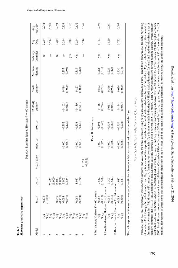
Panel A of Table 2 reports the results of monthly estimations of Equation (3)for our baseline dataset. Each row represents a different regression specifica-tion. To summarize these monthly regressions, we report the average coefficientvalue, along with the percentage of months in which the estimated coefficienthas the same sign as the average coefficient and is significant at the 5% level.This measure of significance should be viewed as only a general indicator of
8 The inclusion of industry dummy variables in our skewness prediction regressions is similar in spirit to theanalysis of Zhang (2005), who computes firm-specific skewness based on the cross-sectional skewness of firmsin the same industry.
9 The results are essentially unchanged if we also include a NASDAQ dummy interacted with turnover.
10 We also estimate models (not reported) that include a measure of leverage, and find the incremental improvementin adjusted-R2 to be relatively small. Since leverage data are not available for many firms in our sample, we optto omit leverage from our skewness prediction model to retain a larger cross-section of firms.
177
at Pennsylvania State University on February 21, 2016
http://rfs.oxfordjournals.org/D
ownloaded from
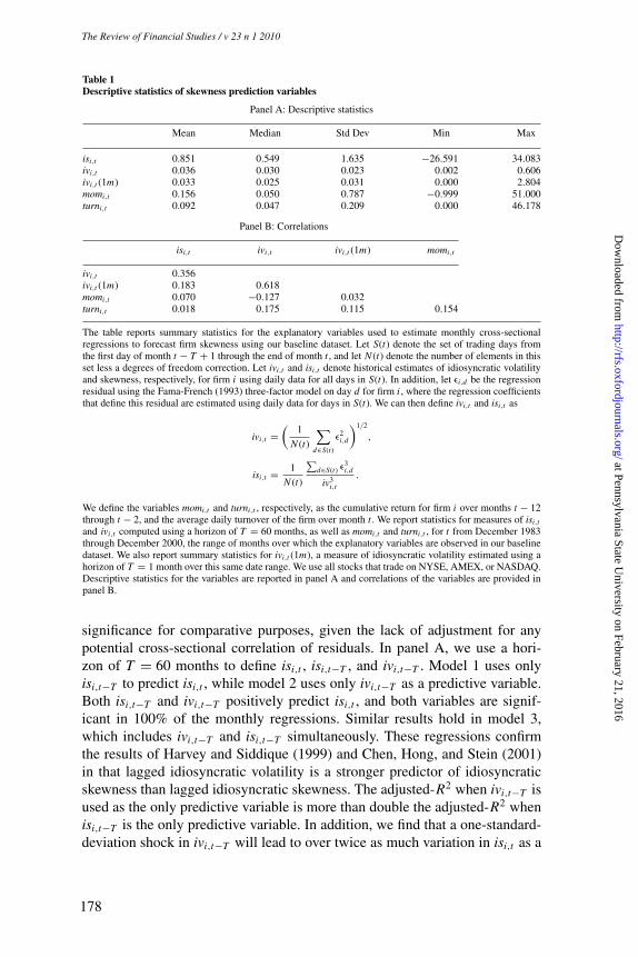
Table 1Descriptive statistics of skewness prediction variables
Panel A: Descriptive statistics
Mean Median Std Dev Min Max
isi,t 0.851 0.549 1.635 −26.591 34.083ivi,t 0.036 0.030 0.023 0.002 0.606ivi,t (1m) 0.033 0.025 0.031 0.000 2.804momi,t 0.156 0.050 0.787 −0.999 51.000turni,t 0.092 0.047 0.209 0.000 46.178
Panel B: Correlations
isi,t ivi,t ivi,t (1m) momi,t
ivi,t 0.356ivi,t (1m) 0.183 0.618momi,t 0.070 −0.127 0.032turni,t 0.018 0.175 0.115 0.154
The table reports summary statistics for the explanatory variables used to estimate monthly cross-sectionalregressions to forecast firm skewness using our baseline dataset. Let S(t) denote the set of trading days fromthe first day of month t − T + 1 through the end of month t , and let N (t) denote the number of elements in thisset less a degrees of freedom correction. Let ivi,t and isi,t denote historical estimates of idiosyncratic volatilityand skewness, respectively, for firm i using daily data for all days in S(t). In addition, let εi,d be the regressionresidual using the Fama-French (1993) three-factor model on day d for firm i , where the regression coefficientsthat define this residual are estimated using daily data for days in S(t). We can then define ivi,t and isi,t as
ivi,t =(
1
N (t)
∑d∈S(t)
ε2i,d
)1/2
,
isi,t = 1
N (t)
∑d∈S(t) ε3
i,d
iv3i,t
.
We define the variables momi,t and turni,t , respectively, as the cumulative return for firm i over months t − 12through t − 2, and the average daily turnover of the firm over month t . We report statistics for measures of isi,t
and ivi,t computed using a horizon of T = 60 months, as well as momi,t and turni,t , for t from December 1983through December 2000, the range of months over which the explanatory variables are observed in our baselinedataset. We also report summary statistics for ivi,t (1m), a measure of idiosyncratic volatility estimated using ahorizon of T = 1 month over this same date range. We use all stocks that trade on NYSE, AMEX, or NASDAQ.Descriptive statistics for the variables are reported in panel A and correlations of the variables are provided inpanel B.
significance for comparative purposes, given the lack of adjustment for anypotential cross-sectional correlation of residuals. In panel A, we use a hori-zon of T = 60 months to define isi,t , isi,t−T , and ivi,t−T . Model 1 uses onlyisi,t−T to predict isi,t , while model 2 uses only ivi,t−T as a predictive variable.Both isi,t−T and ivi,t−T positively predict isi,t , and both variables are signif-icant in 100% of the monthly regressions. Similar results hold in model 3,which includes ivi,t−T and isi,t−T simultaneously. These regressions confirmthe results of Harvey and Siddique (1999) and Chen, Hong, and Stein (2001)in that lagged idiosyncratic volatility is a stronger predictor of idiosyncraticskewness than lagged idiosyncratic skewness. The adjusted-R2 when ivi,t−T isused as the only predictive variable is more than double the adjusted-R2 whenisi,t−T is the only predictive variable. In addition, we find that a one-standard-deviation shock in ivi,t−T will lead to over twice as much variation in isi,t as a
178
The Review of Financial Studies / v 23 n 1 2010
at Pennsylvania State University on February 21, 2016
http://rfs.oxfordjournals.org/D
ownloaded from
Expected Idiosyncratic Skewness
Tabl
e2
Skew
ness
pred
icti
vere
gres
sion
s
Pane
lA:B
asel
ine
data
set;
Hor
izon
T=
60m
onth
s
NA
SDA
QSm
all
Med
ium
Indu
stry
Avg
.A
vgM
odel
isi,
t−T
ivi,
t−T
ivi,
t−T
(1m
)m
omi,
t−T
turn
i,t−
Tdu
mm
ydu
mm
ydu
mm
ydu
mm
ies
Obs
.A
dj.-
R2
1A
vg0.
178
no3,
244
0.04
1%
sig
(1.0
00)
2A
vg20
.423
no3,
244
0.08
9%
sig
(1.0
00)
3A
vg0.
099
18.0
51no
3,24
40.
091
%si
g(0
.935
)(1
.000
)4
Avg
0.08
49.
903
−0.0
01−0
.382
−0.1
620.
814
0.38
5no
3,24
40.
134
%si
g(0
.949
)(0
.834
)(0
.631
)(0
.129
)(0
.613
)(1
.000
)(0
.793
)5
Avg
yes
3,24
40.
026
%si
g6
Avg
0.08
18.
987
−0.0
01−0
.333
−0.1
800.
827
0.38
7ye
s3,
244
0.15
2%
sig
(0.8
94)
(0.7
70)
(0.6
31)
(0.1
20)
(0.5
71)
(1.0
00)
(0.7
82)
7A
vg11
.057
no3,
244
0.04
9%
sig
(0.9
82)
Pane
lB:R
obus
tnes
s8
Full
data
set;
Hor
izon
T=
60m
onth
sA
vg0.
066
7.54
2−0
.001
−0.1
94−0
.116
0.59
20.
281
yes
1,72
30.
097
%si
g(0
.573
)(0
.558
)(0
.325
)(0
.045
)(0
.724
)(0
.783
)(0
.616
)9
Bas
elin
eda
tase
t;H
oriz
onT
=6
mon
ths
Avg
0.05
13.
303
−0.0
01−0
.433
0.01
10.
366
0.22
9ye
s3,
820
0.06
0%
sig
(0.6
46)
(0.5
42)
(0.4
78)
(0.2
62)
(0.0
54)
(0.9
06)
(0.8
68)
10B
asel
ine
data
set;
Hor
izon
T=
24m
onth
sA
vg0.
088
4.08
7−0
.002
−0.5
590.
174
0.62
60.
330
yes
3,72
20.
093
%si
g(0
.806
)(0
.547
)(0
.668
)(0
.221
)(0
.083
)(1
.000
)(0
.913
)
The
tabl
ere
port
sth
etim
e-se
ries
aver
age
ofco
effic
ient
sfr
omm
onth
lycr
oss-
sect
iona
lreg
ress
ions
ofth
efo
rm
isi,
t=
β0,
t+
β1,
tis i
,t−T
+β
2,ti
v i,t
−T+
λ′ tX
i,t−
T+
ε i,t,
whe
reis
i,t
and
ivi,
tar
e,re
spec
tivel
y,id
iosy
ncra
ticsk
ewne
ssan
dvo
latil
ityfo
rfir
mi
estim
ated
usin
gda
ilyex
cess
retu
rns
rela
tive
toa
Fam
a-Fr
ench
thre
e-fa
ctor
mod
elfr
omth
ebe
ginn
ing
ofm
onth
t−T
+1
thro
ugh
the
end
ofm
onth
t,an
dX
i,t−
Tis
ave
ctor
offir
m-s
peci
ficva
riab
les
obse
rvab
leat
the
end
ofm
onth
t−
T.V
aria
bles
inX
i,t−
Tin
clud
em
omi,
t−T
,the
cum
ulat
ive
firm
retu
rnov
erm
onth
st-
T-12
thro
ugh
t-T-
1;tu
rni,
t−T
,firm
turn
over
over
mon
tht-
T;a
dum
my
vari
able
indi
catin
gN
ASD
AQ
stoc
ks;d
umm
ies
for
smal
land
med
ium
-siz
efir
ms;
ase
tof
indu
stry
dum
mie
s;an
div
i,t−
T(1
m),
am
easu
reof
idio
sync
ratic
vola
tility
estim
ated
with
aho
rizo
nof
T=
1m
onth
.Pan
elA
repo
rts
regr
essi
ons
for
our
base
line
data
set,
whi
chin
clud
esst
ocks
that
trad
eon
the
NY
SE,A
ME
X,o
rN
ASD
AQ
and
inw
hich
isi,
t,is
i,t−
T,a
ndiv
i,t−
Tar
ees
timat
edus
ing
aho
rizo
nof
T=
60m
onth
sfo
rt
from
Janu
ary
1988
thro
ugh
Dec
embe
r20
05.P
anel
Bre
port
sro
bust
ness
chec
ksfo
rou
rfu
llda
tase
t(D
ecem
ber
1934
toD
ecem
ber
2005
)an
dfo
ris
i,t,
isi,
t−T,
and
ivi,
t−T
estim
ated
over
hori
zons
ofT
=6
mon
ths
and
T=
24m
onth
s.T
hepe
rcen
tof
coef
ficie
nts
that
are
stat
istic
ally
sign
ifica
ntat
the
5%le
vel(
and
ofth
esa
me
sign
asth
eav
erag
eco
effic
ient
)is
repo
rted
belo
wth
eco
effic
ient
estim
ates
.
179
at Pennsylvania State University on February 21, 2016
http://rfs.oxfordjournals.org/D
ownloaded from
one-standard-deviation shock in isi,t−T . This can be determined using the co-efficients of model 3 along with the standard deviations in Table 1.
Model 4 in panel A includes ivi,t−T , isi,t−T , as well as our other predictivevariables, momi,t−T , turni,t−T , and the dummy variables for NASDAQ firms,small firms, and medium-size firms. Higher values for momi,t−T and turni,t−T areboth associated with lower values of isi,t , consistent with the findings of Chen,Hong, and Stein (2001). The adjusted-R2 of the skewness predictive regressionincreases when the additional variables in model 4 are included. These variableshave fairly consistent statistical significance, although turni,t−T is significant injust 13% of the regressions. The inclusion of these additional variables reducesthe predictive power of ivi,t−T more than isi,t−T , but the estimated impact of aone-standard-deviation shock to ivi,t−T is still more than 60% greater than theestimated impact of a one-standard-deviation shock to isi,t−T .
Model 5 in panel A reports results of regressions including only the industrydummies as explanatory variables and shows that the industry dummies alonehave some ability to predict isi,t . Including the industry dummies along withthe other predictive variables (in model 6) results in the highest adjusted-R2
of any of the regressions. Model 6 is the specification that we focus on in oursubsequent tests. The last model of panel A reports results using a measureof idiosyncratic volatility estimated with a horizon of T = 1 month, ivi,t−T
(1m), to forecast isi,t . These results are included for comparison with Ang etal. (2006, 2008), as discussed in Section 4.
Panel B of Table 2 reports robustness checks of the predictive regressionsreported in panel A. Model 8 uses what we refer to as the “full dataset,”and uses a horizon of T = 60 months to estimate isi,t , isi,t−T , and ivi,t−T .The full dataset includes daily returns for stocks that trade on the NYSE orAMEX from the beginning of January 1925 through December 2005, andstocks that trade on NASDAQ from the beginning of January 1973 throughDecember 2005. As mentioned above, NASDAQ stocks only begin to reportturnover on a widespread basis in January 1983. Hence, when estimating thecross-sectional regressions in Equation (3) using the full dataset for t equal toJanuary 1988 through December 2005, we are able to include turni,t−T and allother explanatory variables as in model 6 of Table 2. For t equal to December1982 through December 1987, we are able to measure isi,t and isi,t−T for allstocks in the cross-section, but we do not observe turni,t−T for stocks thattrade on NASDAQ. Hence, when estimating the cross-sectional regressionsover this period, we omit turni,t−T but include all other explanatory variablesas in model 6. For t equal to December 1934 through November 1982, wecan only use stocks that trade on the NYSE or AMEX, but we use our full setof explanatory variables. Relative to the results in model 6, the results usingthe full dataset generally have smaller estimated coefficients and less-frequentstatistical significance (in part due to the smaller number of observations peryear). However, the signs and relative magnitudes of the coefficients are quitesimilar to the results in model 6.
180
The Review of Financial Studies / v 23 n 1 2010
at Pennsylvania State University on February 21, 2016
http://rfs.oxfordjournals.org/D
ownloaded from
Expected Idiosyncratic Skewness
−2
−1
0
1
2
1930
1935
1940
1945
1950
1955
1960
1965
1970
1975
1980
1985
1990
1995
2000
Est
imat
ed D
umm
y V
aria
ble
UtilitiesTelecomTextiles
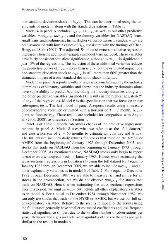
Figure 2Predicted skewness of selected industriesThe time series of estimated industry dummy variables from monthly cross-sectional estimates of our skewnessprediction model described in Equation (3) and as reported in model 8 of Table 2. Dummies for utilities,telecommunications, and textiles industries following Ken French’s industry designations are included.
The last two models in panel B repeat the regressions from model 6 of panelA but use measures of isi,t , isi,t−T , and ivi,t−T with horizons of six months andtwo years. The results are fairly similar in sign and magnitude to the resultsfor the five-year skewness measures. We do observe that the coefficient on theNASDAQ dummy increases in value and decreases in average significance inthese regressions relative to those of panel A.
In Figure 2, we report a time-series plot of some industry dummy variables(from our estimations in model 8 of Table 2) to provide some insight into theirbehavior. We include industry dummies for utilities, telecommunications, andtextiles stocks. The plots of these three series in Figure 2 show substantialtime-series variation for each of the industries; similar variation exists forindustries not included. Much of the variation in these dummy plots appears toconform to expectations. For example, the sign on the utilities industry dummyis almost always negative from the 1940s forward, consistent with the beliefthat this heavily regulated industry offers comparatively little upside potential.The large positive spike in the utilities industry dummy during the late 1930sand early 1940s corresponds to the Natural Gas Act of 1938, which forcedthe splitting up of the utilities industry from a few dominant firms into manysmaller companies. High positive coefficients on telecommunications stocksduring the late 1950s, 1970s, and early 1990s also coincide with periods whenthese types of companies generated positive attention and abnormally largereturns. We include the textiles industry dummy as it represents the industry
181
at Pennsylvania State University on February 21, 2016
http://rfs.oxfordjournals.org/D
ownloaded from
with the largest time-series variation, as evidenced by the large swings in thecoefficient’s value from the 1970s through 2000.
In summary, the results of this section suggest that a simple cross-sectionalmodel including lagged idiosyncratic volatility and skewness, momentum,turnover, size, and industry dummies can help investors to forecast skewness.In the next section, we assess whether idiosyncratic skewness, as predicted bythis model, can help explain the cross-section of expected returns.
3. Expected Skewness and Average Returns
The primary objective of our skewness prediction model is to allow us totest whether expected skewness contributes to our understanding of the cross-section of returns. We conduct standard asset pricing tests and find a strongnegative cross-sectional relation between average returns and expected skew-ness, consistent with the theoretical motivation of Section 1. In this section,we first assess how average returns vary across stocks with differing levels ofexpected skewness. We then turn to the impact of predicted skewness in cross-sectional regressions using the methodology of Fama and MacBeth (1973).
3.1 Portfolios sorted on predicted skewnessWe construct measures of expected skewness at the end of every month in ourbaseline dataset, Et [isi,t+T ], for t equal to January 1988 through November2005, as outlined in Equations (3) and (4). The variables used in the cross-sectional regressions are given in model 6 of Table 2. We then sort stocks intoquintile portfolios at the end of each month based on Et [isi,t+T ], and computethe value-weighted return for each portfolio over month t + 1. Table 3 presentsdescriptive statistics for the five quintiles, where the first quintile representsfirms with the lowest predicted skewness, and the fifth quintile represents firmswith the highest predicted skewness. Column 1 of Table 3 reports the time-series average of the value-weighted portfolio returns. This column shows thatmean returns decline monotonically from the first quintile to the fifth quintile.Mean returns are substantially lower in the fifth quintile (0.52%) compared tothe first quintile (1.19%), a difference of 0.67% per month (t-statistic = 2.91),indicating large differences in average returns for firms with differing levelsof predicted skewness. The largest decline in mean returns occurs between thefourth and fifth quintiles.
While predicted skewness appears to be an important determinant of returns,lagged skewness alone is not a good predictor of returns. In other tests (notreported), we repeat the analysis of Table 3 but sort firms into portfolios basedon measures of predicted skewness that use isi,t−T as the only predictive variable(model 1 of Table 2). In this sorting, mean returns are only slightly lower in thefifth quintile than in the first quintile, with a difference of 0.04% per month.This result is in line with our evidence that additional variables are required toestimate expected skewness in an economically meaningful way.
182
The Review of Financial Studies / v 23 n 1 2010
at Pennsylvania State University on February 21, 2016
http://rfs.oxfordjournals.org/D
ownloaded from

Expected Idiosyncratic Skewness
Table 3Descriptive statistics of portfolios by level of predicted skewness
(2) (4) (5) (7) (8)(1) Standard (3) Firm Firm (6) CAPM FF
Mean deviation Skewness skewness i-vol% Size alpha alpha
1 (Low) 1.189 4.272 −0.604 0.167 1.888 13.596 0.143 0.140(2.13) (2.29)
2 1.115 4.745 −0.789 0.375 2.087 12.950 0.005 −0.005(0.006) −(0.06)
3 1.105 4.972 −0.690 0.565 2.627 11.651 0.005 −0.208(0.04) −(1.63)
4 1.059 5.518 −0.195 0.809 3.406 10.470 0.054 −0.178(0.28) −(1.05)
5 (High) 0.515 6.897 0.219 1.629 5.324 9.404 −0.655 −0.855−(2.21) −(3.79)
1–5 0.674 0.797 0.995(2.91) (2.38) (3.78)
We construct estimates of Et [isi,t+T ] at the end of each month from December 1987 through November 2005as outlined in Equations (3) and (4) of the paper, using a horizon of T = 60 months. The variables used inthe cross-sectional regressions are given in model 6 of Table 2. We then sort stocks into quintile portfolios atthe end of each month based on Et [isi,t+T ] and compute the value-weighted return over month t + 1 for eachportfolio. This table reports descriptive statistics for the five quintiles, where the first quintile represents firmswith the lowest predicted skewness, and the fifth quintile represents firms with the highest predicted skewness.Column 1 reports the time-series average of the value-weighted portfolio returns. Columns 2 and 3 report thetime-series standard deviation and skewness of the portfolio returns. Columns 4, 5, and 6 report averages, acrosstime, of the value-weighted cross-sectional averages of isi,t , ivi,t (1m), and ln(sizei,t ), respectively, within eachportfolio. Columns 7 and 8 report estimated alphas and t-statistics (in parentheses) from the CAPM and theFama-French (1993) three-factor model.
The columns in the middle of Table 3 report other descriptive statistics ofthe predicted-skewness quintiles. Columns 2 and 3 of Table 3 report the time-series standard deviation and skewness of the portfolio returns. Columns 4, 5,and 6 report the averages, across time, of the value-weighted cross-sectionalaverages of isi,t , ivi,t (1m), and ln(sizei,t) within each portfolio, where ln(sizei,t)is the natural log of size for firm i at the end of month t . Average values ofivi,t (1m) increase monotonically from the first quintile to the fifth quintile,indicating a positive relation between ivi,t (1m) and Et [isi,t+T ], consistent withthe predictive regressions of Table 2. We also find that the time-series measuresof portfolio skewness (reported in column 3) increase with predicted skewnessacross the quintiles. We also find that firms with higher predicted skewnesstend to be smaller than firms with lower predicted skewness, consistent withthe results of Table 2.
Most importantly, the last two columns of Table 3 show that the differencesin returns for the expected-skewness quintiles are even greater after adjustingfor risk. We report alphas relative to the CAPM and relative to the Fama-Frenchthree-factor model for each of the quintiles. The difference in the Fama-Frenchalphas is particularly pronounced, with the first quintile having an alpha of0.14% per month and the fifth quintile having an alpha of −0.86% per month,a difference of 1.00% per month. The difference in the alphas of the first andfifth quintiles is highly statistically significant. In summary, Table 3 indicates
183
at Pennsylvania State University on February 21, 2016
http://rfs.oxfordjournals.org/D
ownloaded from
that predicted skewness is negatively related to expected returns, even aftercontrolling for standard measures of risk.
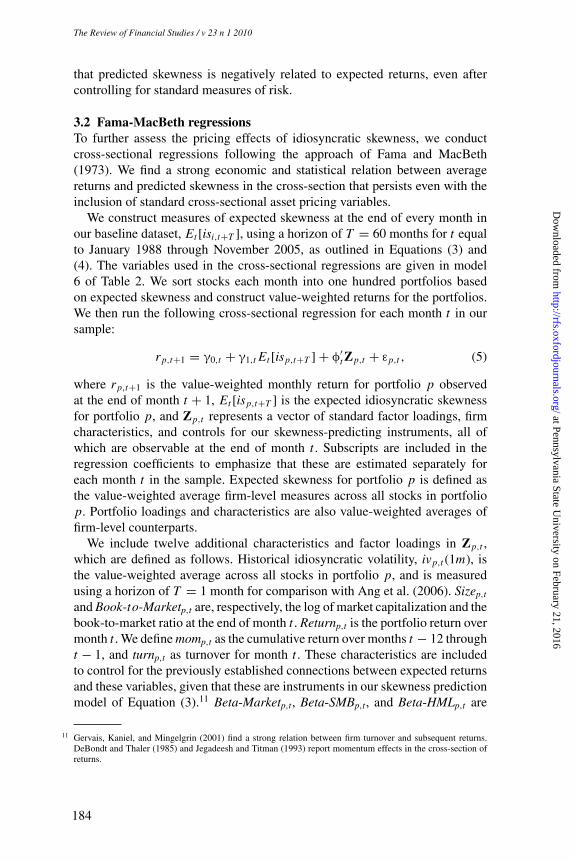
3.2 Fama-MacBeth regressionsTo further assess the pricing effects of idiosyncratic skewness, we conductcross-sectional regressions following the approach of Fama and MacBeth(1973). We find a strong economic and statistical relation between averagereturns and predicted skewness in the cross-section that persists even with theinclusion of standard cross-sectional asset pricing variables.
We construct measures of expected skewness at the end of every month inour baseline dataset, Et [isi,t+T ], using a horizon of T = 60 months for t equalto January 1988 through November 2005, as outlined in Equations (3) and(4). The variables used in the cross-sectional regressions are given in model6 of Table 2. We sort stocks each month into one hundred portfolios basedon expected skewness and construct value-weighted returns for the portfolios.We then run the following cross-sectional regression for each month t in oursample:
rp,t+1 = γ0,t + γ1,t Et [isp,t+T ] + φ′t Zp,t + εp,t , (5)
where rp,t+1 is the value-weighted monthly return for portfolio p observedat the end of month t + 1, Et [isp,t+T ] is the expected idiosyncratic skewnessfor portfolio p, and Zp,t represents a vector of standard factor loadings, firmcharacteristics, and controls for our skewness-predicting instruments, all ofwhich are observable at the end of month t . Subscripts are included in theregression coefficients to emphasize that these are estimated separately foreach month t in the sample. Expected skewness for portfolio p is defined asthe value-weighted average firm-level measures across all stocks in portfoliop. Portfolio loadings and characteristics are also value-weighted averages offirm-level counterparts.
We include twelve additional characteristics and factor loadings in Zp,t ,which are defined as follows. Historical idiosyncratic volatility, ivp,t (1m), isthe value-weighted average across all stocks in portfolio p, and is measuredusing a horizon of T = 1 month for comparison with Ang et al. (2006). Sizep,t
and Book-to-Marketp,t are, respectively, the log of market capitalization and thebook-to-market ratio at the end of month t . Returnp,t is the portfolio return overmonth t . We define momp,t as the cumulative return over months t − 12 throught − 1, and turnp,t as turnover for month t . These characteristics are includedto control for the previously established connections between expected returnsand these variables, given that these are instruments in our skewness predictionmodel of Equation (3).11 Beta-Marketp,t, Beta-SMBp,t, and Beta-HMLp,t are
11 Gervais, Kaniel, and Mingelgrin (2001) find a strong relation between firm turnover and subsequent returns.DeBondt and Thaler (1985) and Jegadeesh and Titman (1993) report momentum effects in the cross-section ofreturns.
184
The Review of Financial Studies / v 23 n 1 2010
at Pennsylvania State University on February 21, 2016
http://rfs.oxfordjournals.org/D
ownloaded from

Expected Idiosyncratic Skewness
the loadings on the Fama-French factors, Beta-UMDp,t is the loading on theCarhart (1997) momentum factor, Beta-Liquidityp,t is the loading on the Pastorand Stambaugh (2003) liquidity factor, and Beta-Coskewp,t is the loading onthe squared excess market return, following Harvey and Siddique (2000). Allloadings are estimated using monthly data from the end of month t − 36 to theend of month t .12
In Table 4, we report the time-series averages of the γ and φ coefficients forour baseline sample, along with t-statistics based on Newey and West (1987)standard errors. Column 1 reports the cross-sectional pricing of expected skew-ness. The coefficient on expected skewness is negative and significant at the1% level. Columns 2–4 include other factor loadings and characteristics as ex-planatory variables. Whether we include the factor loadings only (column 2),the characteristics only (column 3), or both factor loadings and characteristics(column 4), the coefficient on expected skewness remains significant at eitherthe 5% or the 1% level. Including our other explanatory variables in the re-gression will likely lead to a decrease in the significance of expected skewness,given that the expected skewness is a linear combination of a subset of otherexplanatory variables. The coefficients on the other factor loadings and char-acteristics generally conform to expectations and are similar to those in Anget al. (2008). Of particular interest is the fact that the coefficient on idiosyn-cratic volatility is negative as expected, but is not significant at standard levels.Also, in comparison with expected skewness, the t-statistics on the coskewnessloadings are not as large, although the coefficients are negative as predicted.In summary, the results of Table 4 indicate that expected idiosyncratic skew-ness helps to explain the cross-sectional variation in expected returns beyondcommon instruments.
3.2.1 Robustness checks. We conduct a number of robustness checks to theresults of Table 4 and report many of these in Table 5. We vary the number ofportfolios, the data horizon, and the skewness measures to assess the stabilityof the skewness pricing results to these choices. In general, we find that thecoefficient on predicted skewness remains negative and significant in theserobustness checks.
We conduct cross-sectional tests with both fewer and greater numbers ofportfolios relative to our base case. In columns 1 and 2 of Table 5, we repeat theanalysis of Table 4 using fifty portfolios and two hundred portfolios as the testassets. The significance of γ1 is at the 5% level in both cases. The coefficient onidiosyncratic volatility is insignificant in the case of fifty portfolios but signifi-cant in the case of two hundred portfolios. In Section 4, we further disentanglethe separate effects of expected skewness and idiosyncratic volatility.
12 The results in the paper use loadings that are estimated simultaneously, but we find similar results when eachloading is estimated separately.
185
at Pennsylvania State University on February 21, 2016
http://rfs.oxfordjournals.org/D
ownloaded from

Table 4Fama-MacBeth regressions
(1) (2) (3) (4)
Constant 1.527∗∗∗ 1.127∗∗∗ 5.212∗∗ 4.091∗∗(5.05) (3.36) (2.56) (2.16)
Et [isp,t+T ] −0.932∗∗∗ −0.617∗∗ −0.842∗∗∗ −0.624∗∗−(2.66) −(2.28) −(2.84) −(2.16)
ivp,t (1m) −0.189 −0.223−(1.07) −(1.38)
Sizep,t −0.198∗∗ −0.163∗−(1.96) −(1.72)
Book-to-Marketp,t 0.070 0.508(0.14) (1.00)
Returnp,t −0.004 −0.018−(0.20) −(0.81)
momp,t 0.006 0.006(1.27) (1.34)
turnp,t −1.016 −1.586−(0.54) −(0.93)
Beta-Marketp,t 0.265 0.231(0.75) (0.54)
Beta-SMBp,t 0.152 −0.032(0.83) −(0.14)
Beta-HMLp,t 0.048 −0.274(0.21) −(1.17)
Beta-UMDp,t −0.024 0.183−(0.08) (0.70)
Beta-Liquidityp,t 0.636∗ 0.639∗(1.71) (1.72)
Beta-Coskewp,t −6.524∗ −3.378−(1.73) −(0.69)
Adjusted R2 0.085 0.359 0.346 0.490
The table reports results of Fama-MacBeth (1973) regressions, the average coefficients from cross-sectionalregressions,
rp,t+1 = γ0,t + γ1,t Et [isp,t+T ] + φ′t Zp,t + εp,t,
where rp,t+1 is the value-weighted monthly return for portfolio p observed at the end of month t + 1; Et [isp,t+1]is expected idiosyncratic skewness for portfolio p; and Zp,t represents a vector of portfolio loadings andcharacteristics observable at the end of month t . The test assets are one hundred portfolios sorted each monthon Et [isp,t+1]. The regressions are estimated each month using our baseline dataset for t equal to December1987 through November 2005. Expected skewness and other regressors for portfolio p are defined as the value-weighted average firm-level measures across all stocks in portfolio p. We construct measures of Et [isp,t+1]as outlined in Equations (3) and (4) of the paper, using a horizon of T = 60. The variables used in the cross-sectional regressions to estimate Et [isp,t+1] are given in model 6 of Table 2. We also include as a regressorivp,t (1m), the historical idiosyncratic volatility for portfolio p. We estimate ivp,t (1m) as in Equation (2) of thepaper, using a horizon of T = 1 month for comparison with Ang et al. (2006). Sizep,t and Book-to-Marketp,t
are, respectively, the log of market capitalization and book-to-market ratio observed at the end of month t .Returnp,t is the portfolio return over month t ; momp,t is the cumulative return over months t − 12 throught − 2; and turnp,t is turnover over month t . Portfolio loadings and characteristics are also value-weightedaverages of firm-level counterparts using monthly data from the end of month t − 36 to the end of month t .Beta-Marketp,t , Beta-SMBp,t , and Beta-HMLp,t are portfolio loadings on the three Fama-French (1993) factors;Beta-UMDp,t is the portfolio loading on the Carhart (1997) momentum factor; Beta-Liquidityp,t is the loadingon the Pastor-Stambaugh (2003) liquidity factor; and Beta-Coskewp,t is the loading on the squared excessmarket return following Harvey and Siddique (2000). Average coefficients and Newey-West (1987) t-statistics(in parentheses) are reported along with average adjusted-R2. Significance at the 1%, 5%, and 10% level isindicated by ∗∗∗, ∗∗, and ∗, respectively.
186
The Review of Financial Studies / v 23 n 1 2010
at Pennsylvania State University on February 21, 2016
http://rfs.oxfordjournals.org/D
ownloaded from
Expected Idiosyncratic Skewness
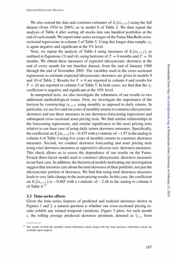
We also extend the data and construct estimates of Et [isi,t+T ] using the fulldataset (from 1934 to 2005), as in model 8 of Table 2. We then repeat theanalysis of Table 4 after sorting all stocks into one hundred portfolios at theend of each month. We report time-series averages of the Fama-MacBeth cross-sectional regressions in column 3 of Table 5. Using this longer data sample, γ1
is again negative and significant at the 5% level.Next, we repeat the analysis of Table 4 using measures of Et [isi,t+T ], as
outlined in Equations (3) and (4), using horizons of T = 6 months and T = 24months. We obtain these measures of expected idiosyncratic skewness at theend of every month for our baseline dataset, from the end of January 1988through the end of November 2005. The variables used in the cross-sectionalregressions to estimate expected idiosyncratic skewness are given in models 9and 10 of Table 2. Results for T = 6 are reported in column 4 and results forT = 24 are reported in column 5 of Table 5. In both cases, we find that the γ1
coefficient is negative and significant at the 10% level.In unreported tests, we also investigate the robustness of our results to two
additional methodological issues. First, we investigate the importance of thehorizon by constructing isi,t+T using monthly as opposed to daily returns. Inparticular, we use five and ten years of monthly returns to construct idiosyncraticskewness and use these measures in our skewness-forecasting regressions andsubsequent cross-sectional asset pricing tests. We find similar relationships inthe forecasting regressions, and similar significance in the asset pricing testsrelative to our base case of using daily return skewness measures. Specifically,the coefficient on Et [isi,t+T ] is −0.435 with a t-statistic of −1.87 in the analog tocolumn 4 of Table 4 using five years of monthly returns to construct skewnessmeasures. Second, we conduct skewness forecasting and asset pricing testsusing total skewness measures as opposed to idiosyncratic skewness measures.This check allows us to assess the dependence of our results on the Fama-French three-factor model used to construct idiosyncratic skewness measuresin our base case. In addition, the theoretical models motivating our investigationsuggest that investors care about the total skewness of their portfolio, not just theidiosyncratic portion of skewness. We find that using total skewness measuresleads to very little change in the asset pricing results. In this case, the coefficienton Et [isi,t+T ] is −0.865 with a t-statistic of −2.48 in the analog to column 4of Table 4.13
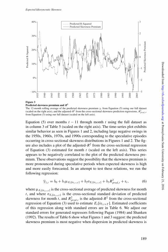
3.3 Time-series effectsGiven the time-series features of predicted and realized skewness shown inFigures 1 and 2, a natural question is whether our cross-sectional pricing re-sults exhibit any related temporal variations. Figure 3 plots, for each montht , the rolling average predicted skewness premium, denoted as γ1,t , from
13 The results of both the monthly return robustness check along with the total skewness robustness check areavailable upon request.
187
at Pennsylvania State University on February 21, 2016
http://rfs.oxfordjournals.org/D
ownloaded from
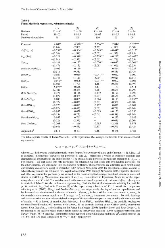
Table 5Fama-MacBeth regressions, robustness checks
(1) (2) (3) (4) (5)Horizon T = 60 T = 60 T = 60 T = 6 T = 24Period 88–05 88–05 34–05 88–05 88–05Number of portfolios 50 200 100 100 100
Constant 4.602∗ 4.576∗∗∗ 2.256∗∗∗ 2.844∗ 5.322∗∗∗(1.84) (2.80) (3.37) (1.80) (3.30)
Et [isp,t+T ] −0.759∗∗ −0.564∗∗ −0.343∗∗ −0.447∗ −0.313∗−(2.24) −(1.99) −(2.02) −(1.92) −(1.85)
ivp,t (1m) −0.221 −0.349∗∗ −0.239∗∗∗ −0.297∗ −0.442∗∗−(1.01) −(2.57) −(2.61) −(1.71) −(2.35)
Sizep,t −0.184 −0.177∗∗ −0.076∗∗ −0.087 −0.201∗∗−(1.47) −(2.15) −(2.08) −(1.06) −(2.53)
Book-to-Marketp,t 0.402 0.169 − 0.414 −0.227(0.51) (0.38) − (0.83) −(0.43)
Returnp,t −0.029 −0.019 −0.041∗∗∗ −0.012 0.000−(1.14) −(1.11) −(3.90) −(0.62) (0.01)
momp,t 0.012∗∗ 0.006∗ 0.011∗∗∗ −0.002 −0.002(1.98) (1.70) (4.48) −(0.38) −(0.49)
turnp,t −5.078∗∗ −0.618 3.471 −1.163 0.514−(2.18) −(0.46) (1.28) −(0.68) (0.29)
Beta-Marketp,t 0.477 0.118 0.132 0.194 −0.290(1.07) (0.36) (0.71) (0.53) −(0.72)
Beta-SMBp,t 0.080 −0.005 0.064 0.113 −0.052∗∗(0.32) −(0.02) (0.57) (0.35) −(0.20)
Beta-HMLp,t −0.270 −0.092 0.172 0.072 −0.009−(0.92) −(0.47) (1.62) (0.27) −(0.04)
Beta-UMDp,t −0.055 0.058 −0.093 −0.155 −0.350−(0.15) (0.27) −(0.64) −(0.58) −(1.04)
Beta-Liquidityp,t 0.055 0.761∗∗ − 0.253 0.082(0.12) (2.39) − (0.63) (0.20)
Beta Coskewp,t −3.308 −1.816 0.985 −2.318 1.974−(0.64) −(0.45) (0.41) −(0.59) (0.42)
Adjusted R2 0.611 0.403 0.461 0.468 0.481
The table reports results of Fama-MacBeth (1973) regressions, the average coefficients from cross-sectionalregressions,
rp,t+1 = γ0,t + γ1,t Et [isp,t+T ] + φ′t Zp,t + εp,t ,
where rp,t+1 is the value-weighted monthly return for portfolio p observed at the end of month t + 1; Et [isp,t+1]is expected idiosyncratic skewness for portfolio p; and Zp,t represents a vector of portfolio loadings andcharacteristics observable at the end of month t . The test assets are portfolios sorted each month on Et [isp,t+1].For column 1, we sort stocks into fifty portfolios; for column 2, we sort stocks into two hundred portfolios; forthe other columns, we sort stocks into one hundred portfolios. The regressions are estimated each month usingour baseline dataset for t equal to December 1987 through November 2005 for all columns except column 3,where the regressions are estimated for t equal to December 1934 through November 2005. Expected skewnessand other regressors for portfolio p are defined as the value-weighted average firm-level measures across allstocks in portfolio p. We construct measures of Et [isp,t+1] as outlined in Equations (3) and (4) of the paper,using a horizon of T = 60. The variables used in the cross-sectional regressions to estimate Et [isp,t+1] are givenin model 6 of Table 2. We also include as a regressor ivp,t (1m), the historical idiosyncratic volatility for portfoliop. We estimate ivp,t (1m) as in Equation (2) of the paper, using a horizon of T = 1 month for comparisonwith Ang et al. (2006). Sizep,t and Book-to-Marketp,t are, respectively, the log of market capitalization andbook-to-market ratio observed at the end of month t . Returnp,t is the portfolio return over month t , momp,t isthe cumulative return over months t − 12 through t − 2, and turnp,t is turnover over month t . Portfolio loadingsand characteristics are also value-weighted averages of firm-level counterparts using monthly data from the endof month t − 36 to the end of month t . Beta-Marketp,t , Beta-SMBp,t , and Beta-HMLp,t are portfolio loadings onthe three Fama-French (1993) factors; Beta-UMDp,t is the portfolio loading on the Carhart (1997) momentumfactor; Beta-Liquidityp,t is the loading on the Pastor-Stambaugh (2003) liquidity factor; and Beta-Coskewp,t isthe loading on the squared excess market return following Harvey and Siddique (2000). Average coefficients andNewey-West (1987) t-statistics (in parentheses) are reported along with average adjusted-R2. Significance at the1%, 5%, and 10% level is indicated by ∗∗∗, ∗∗, and ∗, respectively.
188
The Review of Financial Studies / v 23 n 1 2010
at Pennsylvania State University on February 21, 2016
http://rfs.oxfordjournals.org/D
ownloaded from
Expected Idiosyncratic Skewness
−10%
0%
10%
20%
30%
40%
1935
1940
1945
1950
1955
1960
1965
1970
1975
1980
1985
1990
1995
2000
2005
Pre
dict
ed R
-Squ
ared
Pre
dict
ed S
kew
ness
Pre
miu
m
−3
−2
−1
0
1
2
3Predicted R-SquaredPredicted Skewness Premium
Figure 3Predicted skewness premium and R2
The 12-month rolling average of the predicted skewness premium γt from Equation (5) using our full dataset(scaled on the right axis), and the adjusted-R2 from the cross-sectional skewness prediction regressions, R2
pred,t ,from Equation (3) using our full dataset (scaled on the left axis).
Equation (5) over months t − 11 through month t using the full dataset asin column 3 of Table 5 (scaled on the right axis). The time-series plot exhibitssimilar behavior as seen in Figures 1 and 2, including large negative swings inthe 1950s, 1960s, 1970s, and 1990s corresponding to the speculative episodesoccurring in cross-sectional skewness distributions in Figures 1 and 2. The fig-ure also includes a plot of the adjusted-R2 from the cross-sectional regressionof Equation (3) estimated for month t (scaled on the left axis). This seriesappears to be negatively correlated to the plot of the predicted skewness pre-mium. These observations suggest the possibility that the skewness premium ismore pronounced during speculative periods when expected skewness is highand more easily forecasted. In an attempt to test these relations, we run thefollowing regression:
γ1,t = δ0 + δ1μEt [isi,t+T ] + δ2σEt [isi,t+T ] + δ3 R2pred,t + εt , (6)
where μEt [isi,t+T ] is the cross-sectional average of predicted skewness for montht , and where σEt [isi,t+T ] is the cross-sectional standard deviation of predictedskewness for month t , and R2
pred,t is the adjusted-R2 from the cross-sectionalregression of Equation (3) used to estimate Et [isi,t+T ]. Estimated coefficientsof this regression along with standard errors are in Table 6. We adjust ourstandard errors for generated regressors following Pagan (1984) and Shanken(1992). The results of Table 6 show what Figures 1 and 3 suggest: the predictedskewness premium is most negative when dispersion in predicted skewness is
189
at Pennsylvania State University on February 21, 2016
http://rfs.oxfordjournals.org/D
ownloaded from
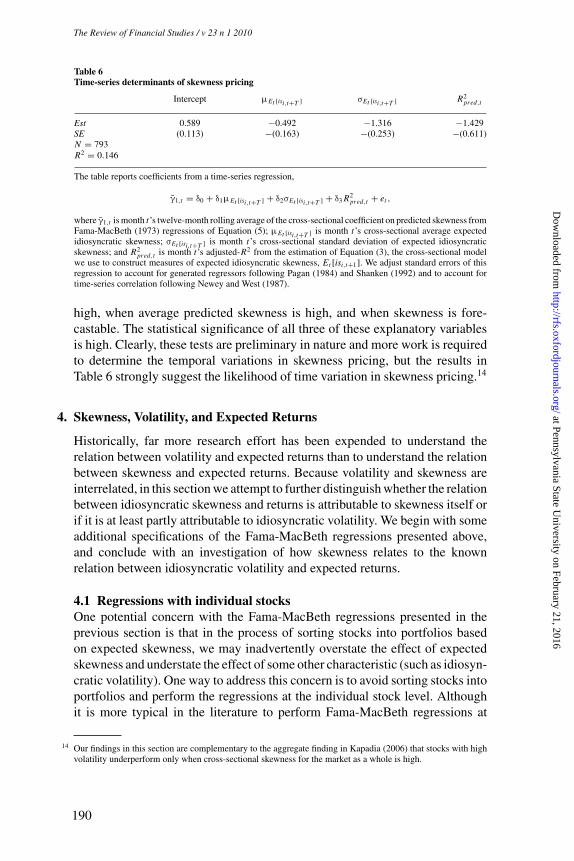
Table 6Time-series determinants of skewness pricing
Intercept μEt [isi,t+T ] σEt [isi,t+T ] R2pred,t
Est 0.589 −0.492 −1.316 −1.429SE (0.113) −(0.163) −(0.253) −(0.611)N = 793R2 = 0.146
The table reports coefficients from a time-series regression,
γ1,t = δ0 + δ1μEt [isi,t+T ] + δ2σEt [isi,t+T ] + δ3 R2pred,t + et ,
where γ1,t is month t’s twelve-month rolling average of the cross-sectional coefficient on predicted skewness fromFama-MacBeth (1973) regressions of Equation (5); μEt [isi,t+T ] is month t’s cross-sectional average expectedidiosyncratic skewness; σEt [isi,t+T ] is month t’s cross-sectional standard deviation of expected idiosyncraticskewness; and R2
pred,t is month t’s adjusted-R2 from the estimation of Equation (3), the cross-sectional modelwe use to construct measures of expected idiosyncratic skewness, Et [isi,t+1]. We adjust standard errors of thisregression to account for generated regressors following Pagan (1984) and Shanken (1992) and to account fortime-series correlation following Newey and West (1987).
high, when average predicted skewness is high, and when skewness is fore-castable. The statistical significance of all three of these explanatory variablesis high. Clearly, these tests are preliminary in nature and more work is requiredto determine the temporal variations in skewness pricing, but the results inTable 6 strongly suggest the likelihood of time variation in skewness pricing.14
4. Skewness, Volatility, and Expected Returns
Historically, far more research effort has been expended to understand therelation between volatility and expected returns than to understand the relationbetween skewness and expected returns. Because volatility and skewness areinterrelated, in this section we attempt to further distinguish whether the relationbetween idiosyncratic skewness and returns is attributable to skewness itself orif it is at least partly attributable to idiosyncratic volatility. We begin with someadditional specifications of the Fama-MacBeth regressions presented above,and conclude with an investigation of how skewness relates to the knownrelation between idiosyncratic volatility and expected returns.
4.1 Regressions with individual stocksOne potential concern with the Fama-MacBeth regressions presented in theprevious section is that in the process of sorting stocks into portfolios basedon expected skewness, we may inadvertently overstate the effect of expectedskewness and understate the effect of some other characteristic (such as idiosyn-cratic volatility). One way to address this concern is to avoid sorting stocks intoportfolios and perform the regressions at the individual stock level. Althoughit is more typical in the literature to perform Fama-MacBeth regressions at
14 Our findings in this section are complementary to the aggregate finding in Kapadia (2006) that stocks with highvolatility underperform only when cross-sectional skewness for the market as a whole is high.
190
The Review of Financial Studies / v 23 n 1 2010
at Pennsylvania State University on February 21, 2016
http://rfs.oxfordjournals.org/D
ownloaded from
Expected Idiosyncratic Skewness
the portfolio level, we conduct these tests at the individual stock level to get asense of whether the aggregation into expected-skewness-sorted portfolios isunduly influencing our results. We therefore run the following cross-sectionalregression for each month t in our sample:
ri,t+1 = γ0,t + γ1,t Et [isi,t+T ] + φ′t Zi,t + εi,t , (7)
where ri,t+1 is the monthly return for firm i observed at the end of month t + 1,and all other variables are as defined in Equation (5) with the exception thatthey are calculated at the individual stock level.
We report the results of our estimation of Equation (7) in Table 7. Column1 reports results with only expected skewness included in the regression. Theγ1 coefficient is negative and significant at the 5% level. In contrast, whenidiosyncratic volatility is included alone in the regression (column 2), thecoefficient on idiosyncratic volatility is negative but not statistically significant.In column 3, we include both expected skewness and idiosyncratic volatilityand the result persists: the coefficient on expected skewness is significant butthe coefficient on idiosyncratic volatility is not. Column 4 reports results withexpected skewness as well as all of our factor loadings. Here the γ1 coefficientremains negative and is significant at the 5% level. In column 5, we includeall other characteristics, including idiosyncratic volatility, and in column 6we include characteristics and factor loadings in the regression. In both ofthese cases, the coefficient on expected skewness is negative and significant atthe 10% level. The coefficient on idiosyncratic volatility is significant at the1% level in both cases.15
In summary, Table 7 shows that although the size of the coefficients is smallerthan in the portfolio-based results, expected idiosyncratic skewness has signif-icant explanatory power in the individual stock setting as well. In comparisonwith idiosyncratic volatility, expected skewness has greater explanatory powerwhen control variables are not included, and idiosyncratic volatility has greaterexplanatory power after including control variables. Given that the expectedskewness variable is a linear combination of control variables, it is not sur-prising that expected skewness loses some explanatory power when all controlvariables are included in the regression. Overall, Table 7 shows that expectedskewness has explanatory power over and above the explanatory power ofidiosyncratic volatility, and that the Fama-MacBeth results reported in the pre-vious section are not unduly affected by sorting stocks on expected skewness.
4.2 Regressions with volatility-sorted portfoliosWe now explore further whether sorting stocks into portfolios based on expectedskewness biases our results in favor of idiosyncratic skewness and againstidiosyncratic volatility. We perform Fama-MacBeth regressions in which we
15 In unreported regressions, we also perform Fama-MacBeth regresssions at the individual stock level in whichinstead of using lagged iv as an explanatory variable we use predicted iv. We use the same explanatory variablesfor predicted iv as we use in our skewness prediction model. In these regressions predicted iv is never significant,whereas predicted skewness remains significant.
191
at Pennsylvania State University on February 21, 2016
http://rfs.oxfordjournals.org/D
ownloaded from
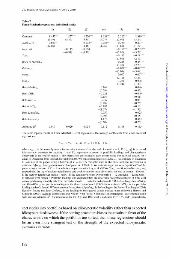
Table 7Fama-MacBeth regressions, individual stocks
(1) (2) (3) (4) (5) (6)
Constant 1.455∗∗∗ 1.257∗∗∗ 1.520∗∗∗ 1.034∗∗∗ 3.262∗∗∗ 2.919∗∗∗(5.19) (5.39) (5.81) (4.77) (2.90) (3.24)
Et [isi,t+T ] −0.669∗∗ −0.633∗∗ −0.384∗∗ −0.350∗ −0.297∗−(2.05) −(2.16) −(1.96) −(1.82) −(1.77)
ivi,t (1m) −0.115 −0.094 −0.188∗∗∗ −0.205∗∗∗−(0.91) −(0.79) −(2.80) −(3.79)
Sizei,t −0.115∗ −0.111∗∗−(1.90) −(2.19)
Book-to-Marketi,t 0.216 0.281∗∗(1.28) (2.23)
Returni,t −0.021∗∗∗ −0.027∗∗∗−(3.01) −(3.68)
momi,t 0.007∗∗∗ 0.007∗∗∗(2.72) (3.23)
turni,t 1.251 0.908(1.24) (1.33)
Beta-Marketi,t 0.168 0.096(0.79) (0.47)
Beta-SMBi,t −0.021 −0.049−(0.15) −(0.41)
Beta-HMLi,t 0.049 −0.041(0.28) −(0.26)
Beta-UMDi,t −0.182 −0.181−(1.07) −(1.36)
Beta-Liquidityi,t 0.059 −0.025(0.30) −(0.15)
Beta-Coskewi,t −1.175 0.453−(0.60) (0.25)
Adjusted R2 0.017 0.029 0.038 0.112 0.108 0.155
The table reports results of Fama-MacBeth (1973) regressions, the average coefficients from cross-sectionalregressions,
ri,t+1 = γ0,t + γ1,t Et [isi,t+T ] + φ′t Zi,t + εi,t,
where ri,t+1 is the monthly return for security i observed at the end of month t + 1, Et [isi,t+1] is expectedidiosyncratic skewness for security i , and Zi,t represents a vector of portfolio loadings and characteristicsobservable at the end of month t . The regressions are estimated each month using our baseline dataset for tequal to December 1987 through November 2005. We construct measures of Et [isi,t+1] as outlined in Equations(3) and (4) of the paper, using a horizon of T = 60. The variables used in the cross-sectional regressions toestimate Et [isi,t+1] are given in model 6 of panel A of Table 2. We estimate ivi,t (1m) as in Equation (2) of thepaper using a horizon of T = 1 month for comparison with Ang et al. (2006). Sizei,t and Book-to-Marketi,t are,respectively, the log of market capitalization and book-to-market ratio observed at the end of month t . Returni,t
is the security return over month t , momi,t is the cumulative return over months t − 12 through t − 2, and turni,t
is turnover over month t . Portfolio loadings and characteristics are also value-weighted averages of firm-levelcounterparts using monthly data from the end of month t − 36 to the end of month t . Beta-Marketi,t , Beta-SMBi,t ,and Beta-HMLi,t are portfolio loadings on the three Fama-French (1993) factors; Beta-UMDi,t , is the portfolioloading on the Carhart (1997) momentum factor; Beta-Liquidityi,t is the loading on the Pastor-Stambaugh (2003)liquidity factor; and Beta-Coskewi,t is the loading on the squared excess market return following Harvey andSiddique (2000). Average coefficients and Newey-West (1987) t-statistics (in parentheses) are reported alongwith average adjusted-R2. Significance at the 1%, 5%, and 10% level is indicated by ∗∗∗, ∗∗, and ∗, respectively.
sort stocks into portfolios based on idiosyncratic volatility rather than expectedidiosyncratic skewness. If the sorting procedure biases the results in favor of thecharacteristic on which the portfolios are sorted, then these regressions shouldbe an even more stringent test of the strength of the expected idiosyncraticskewness variable.
192
The Review of Financial Studies / v 23 n 1 2010
at Pennsylvania State University on February 21, 2016
http://rfs.oxfordjournals.org/D
ownloaded from
Expected Idiosyncratic Skewness
We perform regressions as above in Equation (5) with the exception thatwe sort stocks each month into one hundred portfolios based on idiosyncraticvolatility instead of expected skewness. The results of the regressions arereported in Table 8. The coefficients reported in the first three columns showa similar pattern as in Table 7. When included alone in the regression thecoefficient on expected skewness is negative and significant and the coefficienton idiosyncratic volatility is not significant. In column 3, when we include bothvariables, neither coefficient is significant. In the last three columns, we reportresults of regressions including the factor loadings and characteristics. In theseregressions, the coefficient on expected skewness is significant at the 5% levelin every case, while the coefficient on idiosyncratic volatility is significant atthe 1% level. Table 8 shows that the significant explanatory power of expectedidiosyncratic skewness is not dependent on the sorting procedure used, andthat expected skewness has explanatory power distinct from the explanatorypower of idiosyncratic volatility even when idiosyncratic volatility is used asthe sorting variable when forming portfolios.
4.3 Skewness and the idiosyncratic volatility puzzleHaving documented pricing effects of idiosyncratic skewness, we now assesswhether idiosyncratic skewness can help explain the negative relation betweenidiosyncratic volatility and expected returns, as documented by Ang et al.(2006). In doing so, we also hope to further disentangle the separate effectsof idiosyncratic skewness and idiosyncratic volatility on expected returns. Per-haps because a negative relation between risk and return is difficult to reconcilewith standard assumptions regarding investor utility, other explanations for theiv puzzle tend to focus on market imperfections that could induce such a rela-tion, such as short-sale constraints or a lack of information disclosure (Boehmeet al. 2005; Duan, Hu, and McLean 2006; Jiang, Xu, and Yao 2008). In con-trast, an explanation for the iv puzzle based on skewness preference does notfocus on the existence of market imperfections. If investors have a prefer-ence for positive skewness, they may accept lower average returns on stockswith high idiosyncratic volatility if those stocks also offer highly skewedreturns.
Ang et al. (2008) address the potential impact of idiosyncratic skewness onthe negative relation between idiosyncratic volatility and returns. They findthat skewness has a strong negative cross-sectional correlation with expectedreturns. In terms of statistical significance, they show that the negative rela-tion between lagged skewness and returns is even stronger than the negativerelation between lagged idiosyncratic volatility and returns. At the same time,these authors show that the iv puzzle persists even after controlling for laggedskewness. However, Ang et al. (2008) only use lagged skewness as their mea-sure of expected skewness. Since other variables are also important predictorsof skewness, these authors may underestimate the true impact of skewness
193
at Pennsylvania State University on February 21, 2016
http://rfs.oxfordjournals.org/D
ownloaded from
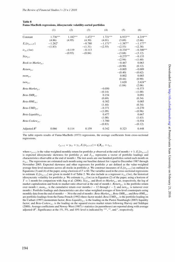
Table 8Fama-MacBeth regressions, idiosyncratic volatility-sorted portfolios
(1) (2) (3) (4) (5) (6)
Constant 1.736∗∗∗ 1.182∗∗∗ 1.472∗∗∗ 1.721∗∗∗ 6.933∗∗∗ 4.219∗∗∗(4.86) (4.95) (4.30) (4.01) (3.69) (2.66)
Et [isp,t+T ] −1.262∗ −0.780 −1.171∗∗ −1.387∗∗ −1.177∗∗−(1.83) −(1.31) −(2.55) −(2.53) −(2.38)
ivp,t (1m) −0.119 −0.113 −0.334∗∗∗ −0.300∗∗∗−(0.93) −(0.84) −(3.68) −(3.12)
Sizep,t −0.275∗∗∗ −0.133−(2.94) −(1.60)
Book-to-Marketp,t −0.467 0.063−(0.90) (0.12)
Returnp,t −0.005 −0.009−(0.40) −(0.62)
momp,t 0.002 0.003(0.44) (0.90)
turnp,t 1.620 2.624∗∗(1.04) (2.06)
Beta-Marketp,t −0.050 −0.373−(0.14) −(1.00)
Beta-SMBp,t 0.154 0.091(0.69) (0.34)
Beta-HMLp,t 0.302 0.085(1.44) (0.34)
Beta-UMDp,t −0.371 −0.270−(1.09) −(0.96)
Beta-Liquidityp,t 0.477 0.667(1.08) (1.63)
Beta-Coskewp,t −3.700 −0.554−(0.83) −(0.12)
Adjusted R2 0.066 0.114 0.159 0.342 0.323 0.448
The table reports results of Fama-MacBeth (1973) regressions, the average coefficients from cross-sectionalregressions,
rp,t+1 = γ0,t + γ1,t Et [isp,t+T ] + φ′t Zp,t + εp,t,
where rp,t+1 is the value-weighted monthly return for portfolio p observed at the end of month t + 1; Et [isp,t+1]is expected idiosyncratic skewness for portfolio p; and Z p,t represents a vector of portfolio loadings andcharacteristics observable at the end of month t . The test assets are one hundred portfolios sorted each month onivp,t . The regressions are estimated each month using our baseline dataset for t equal to December 1987 throughNovember 2005. Expected skewness and other regressors for portfolio p are defined as the value-weightedaverage firm-level measures across all stocks in portfolio p. We construct measures of Et [isp,t+1] as outlined inEquations (3) and (4) of the paper, using a horizon of T = 60. The variables used in the cross-sectional regressionsto estimate Et [isp,t+1] are given in model 6 of Table 2. We also include as a regressor ivp,t (1m), the historicalidiosyncratic volatility for portfolio p. We estimate ivp,t (1m) as in Equation (2) of the paper, using a horizon ofT = 1 month for comparison with Ang et al. (2006). Sizep,t and Book-to-Marketp,t are, respectively, the log ofmarket capitalization and book-to-market ratio observed at the end of month t . Returnp,t is the portfolio returnover month t ; momp,t is the cumulative return over months t − 12 through t − 2; and turnp,t is turnover overmonth t . Portfolio loadings and characteristics are also value-weighted averages of firm-level counterparts usingmonthly data from the end of month t − 36 to the end of month t . Beta-Marketp,t , Beta-SMBp,t , and Beta-HMLp,t
are portfolio loadings from the Fama-French (1992) three-factor model; Beta-UMDp,t is the portfolio loading onthe Carhart (1997) momentum factor; Beta-Liquidityp,t is the loading on the Pastor-Stambaugh (2003) liquidityfactor; and Beta-Coskewp,t is the loading on the squared excess market return following Harvey and Siddique(2000). Average coefficients and Newey-West (1987) t-statistics (in parentheses) are reported along with averageadjusted-R2. Significance at the 1%, 5%, and 10% level is indicated by ∗∗∗, ∗∗, and ∗, respectively.
194
The Review of Financial Studies / v 23 n 1 2010
at Pennsylvania State University on February 21, 2016
http://rfs.oxfordjournals.org/D
ownloaded from
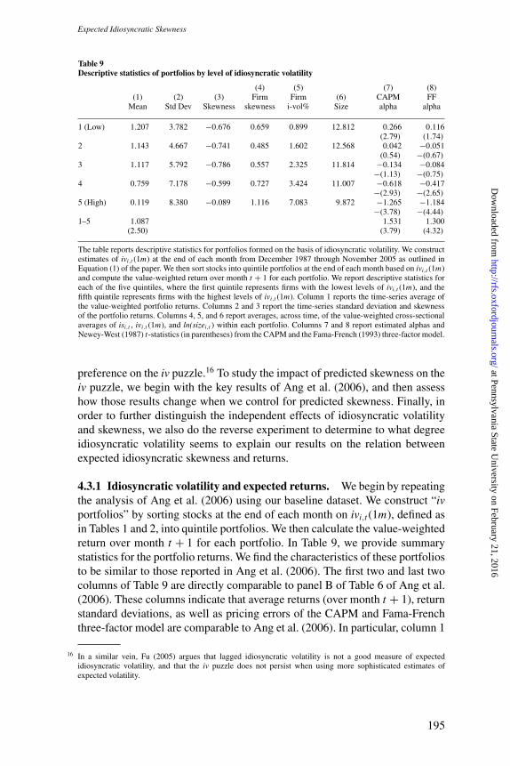
Expected Idiosyncratic Skewness
Table 9Descriptive statistics of portfolios by level of idiosyncratic volatility
(4) (5) (7) (8)(1) (2) (3) Firm Firm (6) CAPM FF
Mean Std Dev Skewness skewness i-vol% Size alpha alpha
1 (Low) 1.207 3.782 −0.676 0.659 0.899 12.812 0.266 0.116(2.79) (1.74)
2 1.143 4.667 −0.741 0.485 1.602 12.568 0.042 −0.051(0.54) −(0.67)
3 1.117 5.792 −0.786 0.557 2.325 11.814 −0.134 −0.084−(1.13) −(0.75)
4 0.759 7.178 −0.599 0.727 3.424 11.007 −0.618 −0.417−(2.93) −(2.65)
5 (High) 0.119 8.380 −0.089 1.116 7.083 9.872 −1.265 −1.184−(3.78) −(4.44)
1–5 1.087 1.531 1.300(2.50) (3.79) (4.32)
The table reports descriptive statistics for portfolios formed on the basis of idiosyncratic volatility. We constructestimates of ivi,t (1m) at the end of each month from December 1987 through November 2005 as outlined inEquation (1) of the paper. We then sort stocks into quintile portfolios at the end of each month based on ivi,t (1m)and compute the value-weighted return over month t + 1 for each portfolio. We report descriptive statistics foreach of the five quintiles, where the first quintile represents firms with the lowest levels of ivi,t (1m), and thefifth quintile represents firms with the highest levels of ivi,t (1m). Column 1 reports the time-series average ofthe value-weighted portfolio returns. Columns 2 and 3 report the time-series standard deviation and skewnessof the portfolio returns. Columns 4, 5, and 6 report averages, across time, of the value-weighted cross-sectionalaverages of isi,t , ivi,t (1m), and ln(sizei,t ) within each portfolio. Columns 7 and 8 report estimated alphas andNewey-West (1987) t-statistics (in parentheses) from the CAPM and the Fama-French (1993) three-factor model.
preference on the iv puzzle.16 To study the impact of predicted skewness on theiv puzzle, we begin with the key results of Ang et al. (2006), and then assesshow those results change when we control for predicted skewness. Finally, inorder to further distinguish the independent effects of idiosyncratic volatilityand skewness, we also do the reverse experiment to determine to what degreeidiosyncratic volatility seems to explain our results on the relation betweenexpected idiosyncratic skewness and returns.
4.3.1 Idiosyncratic volatility and expected returns. We begin by repeatingthe analysis of Ang et al. (2006) using our baseline dataset. We construct “ivportfolios” by sorting stocks at the end of each month on ivi,t (1m), defined asin Tables 1 and 2, into quintile portfolios. We then calculate the value-weightedreturn over month t + 1 for each portfolio. In Table 9, we provide summarystatistics for the portfolio returns. We find the characteristics of these portfoliosto be similar to those reported in Ang et al. (2006). The first two and last twocolumns of Table 9 are directly comparable to panel B of Table 6 of Ang et al.(2006). These columns indicate that average returns (over month t + 1), returnstandard deviations, as well as pricing errors of the CAPM and Fama-Frenchthree-factor model are comparable to Ang et al. (2006). In particular, column 1
16 In a similar vein, Fu (2005) argues that lagged idiosyncratic volatility is not a good measure of expectedidiosyncratic volatility, and that the iv puzzle does not persist when using more sophisticated estimates ofexpected volatility.
195
at Pennsylvania State University on February 21, 2016
http://rfs.oxfordjournals.org/D
ownloaded from
of Table 9 illustrates the poor average performance of the high-iv quintileportfolio. Whereas the low-iv quintile has mean returns of 1.21% per month,the high-iv quintile has mean returns of 0.12% per month. In addition, the lasttwo columns show large pricing errors of the CAPM and the Fama-Frenchmodel. The difference in the Fama-French alphas between the first and fifthquintiles is 1.30% per month. Table 9 shows, similar to Ang et al. (2006), thatthe iv puzzle is most pronounced in the high-iv quintile, where mean returnsand alphas are disproportionately low relative to the other four quintiles.
We also include two skewness variables in Table 9. The first skewness vari-able, in column 3, is the time-series skewness estimate of the respective quintileportfolio returns. While this statistic is negative across all portfolios, quintilesof higher idiosyncratic volatility exhibit less negative levels of skewness in theirreturns. The other skewness variable, firm skewness (in column 4), is the aver-age across time of the value-weighted cross-sectional average of isi,t for eachportfolio, estimated as described in Equation (2) using a horizon of T = 60months.17 The pattern of increasing firm skewness in quintiles with highervolatility again illustrates a strong contemporaneous relation between idiosyn-cratic volatility and idiosyncratic skewness. These two measures of skewnesssuggest that lagged idiosyncratic volatility is related to the skewness of port-folio returns.18 Consistent with the results for the mean returns, the largestincrease in skewness occurs between the fourth and fifth quintiles. Columns 5and 6 report the averages, across time, of the value-weighted cross-sectional av-erages of ivi,t (1m) and ln(si zei,t ) within each portfolio. The relations betweenidiosyncratic volatility, idiosyncratic skewness, and size are consistent withskewness-preferring investors taking speculative positions in small firms withhighly skewed returns and accepting lower average returns in their positionsfor a chance of hitting an investment “home run.”
4.3.2 Conditional sorting. We next directly address the question of whetherpredicted skewness can help explain the iv puzzle. Following the methodologyin Ang et al. (2006, 2008), we conduct a double-sorting exercise to controlfor expected skewness. At the end of each month in our baseline dataset fromJanuary 1988 through November 2005, we first sort firms into five Et [isi,t+T ]quintiles, where we measure Et [isi,t+T ] as in Equations (3) and (4) using a hori-zon of T = 60 months. The variables we use in the cross-sectional regressionof Equation (3) are those used in model 6 of Table 2. Then, for each Et [isi,t+T ]quintile, we sort firms into five “ivc portfolios,” using ivi,t (1m) as above, wherethe superscript c denotes conditional sorting. Within each of these twenty-five
17 We use a horizon of T = 1 to compute ivi,t (1m) to be consistent with the results of Ang et al. (2006, 2008). Weuse a horizon of T = 60 to compute isi,t , consistent with earlier work in our paper. Our results are qualitativelyrobust to using other horizons of T in measuring both isi,t and ivi,t .
18 Return skewness is comprised of idiosyncratic skewness and other coskewness components. Table 2 showsthat idiosyncratic volatility forecasts idiosyncratic skewness, but without further analysis we do not know ifidiosyncratic volatility forecasts other coskewness terms.
196
The Review of Financial Studies / v 23 n 1 2010
at Pennsylvania State University on February 21, 2016
http://rfs.oxfordjournals.org/D
ownloaded from
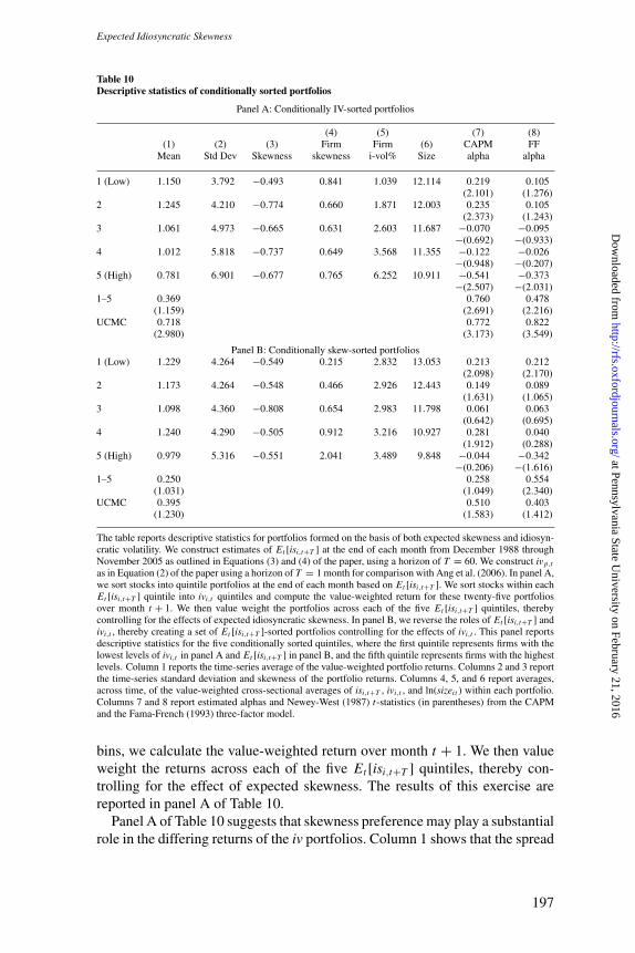
Expected Idiosyncratic Skewness
Table 10Descriptive statistics of conditionally sorted portfolios
Panel A: Conditionally IV-sorted portfolios
(4) (5) (7) (8)(1) (2) (3) Firm Firm (6) CAPM FF
Mean Std Dev Skewness skewness i-vol% Size alpha alpha
1 (Low) 1.150 3.792 −0.493 0.841 1.039 12.114 0.219 0.105(2.101) (1.276)
2 1.245 4.210 −0.774 0.660 1.871 12.003 0.235 0.105(2.373) (1.243)
3 1.061 4.973 −0.665 0.631 2.603 11.687 −0.070 −0.095−(0.692) −(0.933)
4 1.012 5.818 −0.737 0.649 3.568 11.355 −0.122 −0.026−(0.948) −(0.207)
5 (High) 0.781 6.901 −0.677 0.765 6.252 10.911 −0.541 −0.373−(2.507) −(2.031)
1–5 0.369 0.760 0.478(1.159) (2.691) (2.216)
UCMC 0.718 0.772 0.822(2.980) (3.173) (3.549)
Panel B: Conditionally skew-sorted portfolios1 (Low) 1.229 4.264 −0.549 0.215 2.832 13.053 0.213 0.212
(2.098) (2.170)2 1.173 4.264 −0.548 0.466 2.926 12.443 0.149 0.089
(1.631) (1.065)3 1.098 4.360 −0.808 0.654 2.983 11.798 0.061 0.063
(0.642) (0.695)4 1.240 4.290 −0.505 0.912 3.216 10.927 0.281 0.040
(1.912) (0.288)5 (High) 0.979 5.316 −0.551 2.041 3.489 9.848 −0.044 −0.342
−(0.206) −(1.616)1–5 0.250 0.258 0.554
(1.031) (1.049) (2.340)UCMC 0.395 0.510 0.403
(1.230) (1.583) (1.412)
The table reports descriptive statistics for portfolios formed on the basis of both expected skewness and idiosyn-cratic volatility. We construct estimates of Et [isi,t+T ] at the end of each month from December 1988 throughNovember 2005 as outlined in Equations (3) and (4) of the paper, using a horizon of T = 60. We construct ivp,t
as in Equation (2) of the paper using a horizon of T = 1 month for comparison with Ang et al. (2006). In panel A,we sort stocks into quintile portfolios at the end of each month based on Et [isi,t+T ]. We sort stocks within eachEt [isi,t+T ] quintile into ivi,t quintiles and compute the value-weighted return for these twenty-five portfoliosover month t + 1. We then value weight the portfolios across each of the five Et [isi,t+T ] quintiles, therebycontrolling for the effects of expected idiosyncratic skewness. In panel B, we reverse the roles of Et [isi,t+T ] andivi,t , thereby creating a set of Et [isi,t+T ]-sorted portfolios controlling for the effects of ivi,t . This panel reportsdescriptive statistics for the five conditionally sorted quintiles, where the first quintile represents firms with thelowest levels of ivi,t in panel A and Et [isi,t+T ] in panel B, and the fifth quintile represents firms with the highestlevels. Column 1 reports the time-series average of the value-weighted portfolio returns. Columns 2 and 3 reportthe time-series standard deviation and skewness of the portfolio returns. Columns 4, 5, and 6 report averages,across time, of the value-weighted cross-sectional averages of isi,t+T , ivi,t , and ln(sizeit ) within each portfolio.Columns 7 and 8 report estimated alphas and Newey-West (1987) t-statistics (in parentheses) from the CAPMand the Fama-French (1993) three-factor model.
bins, we calculate the value-weighted return over month t + 1. We then valueweight the returns across each of the five Et [isi,t+T ] quintiles, thereby con-trolling for the effect of expected skewness. The results of this exercise arereported in panel A of Table 10.
Panel A of Table 10 suggests that skewness preference may play a substantialrole in the differing returns of the iv portfolios. Column 1 shows that the spread
197
at Pennsylvania State University on February 21, 2016
http://rfs.oxfordjournals.org/D
ownloaded from
of average returns across the conditionally sorted ivc portfolios is much smallerthan in the unconditionally sorted iv quintiles. The return premium between thefirst and fifth portfolios is only 0.37% per month and is no longer significant,down from the 1.09% spread found in Table 9. The iv puzzle of Ang et al. (2006)is substantially reduced when we control for expected idiosyncratic skewness.
Columns 2 and 3 of panel A of Table 10 report the time-series standarddeviation and skewness of the conditionally sorted portfolio returns. Columns4, 5, and 6 report the averages, across time, of the value-weighted cross-sectional averages of isi,t , ivi,t (1m), and ln(sizei,t ) within each portfolio. Wefind relatively small variations in portfolio skewness across the five ivc quintileportfolios, indicating that our model of expected skewness predicts skewnessreasonably well. The average firm skewness measures also show relativelysmall differences relative to the variation found in the unconditionally sorted ivportfolios in Table 9. In fact, firm skewness is now slightly lower in the high-ivc
quintile relative to the low-ivc quintile. However, we still find a wide spread inidiosyncratic volatility across the portfolios. The spread is comparable to thatof the portfolios unconditionally sorted on idiosyncratic volatility reported inTable 9, although volatility is lower in the fifth quintile compared with Table 9.
Finally, in columns 7 and 8 of panel A of Table 10, we control for risk tosee if material pricing differences are found across the quintile portfolios. Wereport alphas relative to the CAPM and relative to the Fama-French three-factormodel for each of the conditionally sorted portfolios. The high-ivc portfoliohas a CAPM intercept estimate of −0.54%, which is significant with a t-statistic of 2.5, indicating that on a CAPM risk-adjusted basis, the iv puzzlestill persists. However, this point estimate is less than half the magnitude of theestimate for the unconditionally sorted high-iv quintile in Table 9. Similarly,the high-ivc portfolio results in panel A of Table 10 indicate a Fama-Frenchintercept of −0.37% on the high-ivc portfolio, which is small relative to the−1.18% intercept for the unconditionally sorted high-iv quintile in Table 9.The evidence indicates that idiosyncratic volatility generates much smallerdifferences in pricing errors relative to the CAPM and Fama-French modelsafter controlling for idiosyncratic skewness.
In the bottom row of panel A of Table 10, we report results from constructing adifference-in-differences portfolio, UCMC (unconditional minus conditional),to better assess the improvements associated with forecasting skewness. Inparticular, we take a long position in the zero-investment iv-sorted long/shortportfolio and a short position in the zero-investment ivc-sorted long/short port-folio. (The iv-sorted long/short portfolio is constructed by taking a long positionin the low-iv quintile portfolio and shorting the high-iv quintile portfolio, andthe ivc-sorted long/short portfolio is constructed by taking a long position inthe low-ivc quintile portfolio and shorting the high-ivc quintile portfolio.) Theresulting difference-in-differences portfolio should allow us to formally test theability of expected skewness to explain the iv puzzle. The results are stronglysupportive of the explanatory power of predicted skewness. The CAPM alpha
198
The Review of Financial Studies / v 23 n 1 2010
at Pennsylvania State University on February 21, 2016
http://rfs.oxfordjournals.org/D
ownloaded from

Expected Idiosyncratic Skewness
on the UCMC portfolio is 0.77% with a t-statistic of 3.2 and the Fama-Frenchthree-factor model has an intercept of 0.82% with a t-statistic of 3.5.
In panel B of Table 10, we repeat the analysis of panel A, except that wereverse the roles of expected skewness and idiosyncratic volatility. Thus, wecontrol for the effect of iv in the expected skewness-sorted portfolios to see ifiv helps explain the differing returns of the expected skewness quintile port-folios as reported in Table 3. The results in panel B show that controlling foriv does reduce the magnitude of the difference in returns between the low-and high-skewness quintiles. Compared to Table 3, the differences in returnsand CAPM alphas between the low and high portfolios are no longer signif-icant. However, the difference between the Fama-French alphas on the lowand high portfolios remains significant, with a t-statistic of 2.3. The magnitudeof the difference indicates that the Fama-French alpha of the low-skewnessquintile exceeds the alpha of the high-skewness quintile by 0.55% per month,even after controlling for iv. The final row of panel B reports the results ofa UCMC portfolio constructed as described for panel A, but with the rolesof expected skewness and idiosyncratic volatility reversed. In contrast to theresults in panel A, the alphas on this UCMC portfolio are not significant at stan-dard levels. Thus, although controlling for iv has some impact on the results inTable 3, the insignificant UCMC portfolio alphas suggest that the changesinduced by idiosyncratic volatility are not statistically significant. By this mea-sure at least, expected idiosyncratic skewness appears to explain the negativerelation between idiosyncratic volatility and returns better than idiosyncraticvolatility explains the negative relation between expected skewness and returns.
4.3.3 Discussion. The results in Table 10 suggest that idiosyncratic skewnessis important in explaining the low average returns of stocks with high idiosyn-cratic volatility. At the same time, these results show that, looking at thingsfrom the other direction, idiosyncratic volatility explains part of our finding thatexpected idiosyncratic skewness is negatively correlated with returns. In eithercase, the significant explanatory power of one of the variables remains aftercontrolling for the other.19 In addition, there is some “overlapping” explanatorypower that could be attributed to either variable. Empirically, it may be difficultto determine whether this overlapping explanatory power should be properlyattributed to volatility or skewness. From a theoretical perspective, however,the skewness explanation appears to have the upper hand, given that there arealready established theoretical explanations for the negative relation betweenidiosyncratic skewness and expected returns (i.e., Barberis and Huang 2007;Brunnermeier and Parker 2005; Mitton and Vorkink 2007). The iv puzzle, by
19 We find consistent results in other tests (not reported) in which we independently sort stocks on expectedskewness and idiosyncratic volatility, thus forming twenty-five portfolios reflecting stocks’ ranking in skewnessand volatility. These results show that, although the changes are not always monotonic across quintiles, alphasare generally lower for the higher-skewness quintiles (across a given iv portfolio) and alphas are generally lowerfor the higher-iv portfolios (across a given skewness portfolio).
199
at Pennsylvania State University on February 21, 2016
http://rfs.oxfordjournals.org/D
ownloaded from
contrast, is an interesting anomaly for which a complete explanation is stillbeing sought.
To the extent that expected skewness explains the iv puzzle, this explana-tion is not mutually exclusive of other explanations of the iv puzzle based onmarket imperfections. To the contrary, we view the skewness-preference expla-nation as complementary to explanations that focus on short-sale constraints ordifferences of opinion. High valuations driven by underdiversified, skewness-preferring investors are more likely to persist when the costs of short selling arehigh. Similarly, large dispersion of opinion may imply greater heterogeneityin skewness preference, with underdiversified investors valuing the upside po-tential of a stock more than similarly informed well-diversified investors withless preference for skewness. Multiple factors may contribute to the iv puzzle,but skewness preference adds a critical element of explaining why some in-vestors place high value on stocks with high past idiosyncratic risk in the firstplace.
5. Conclusion
Although a number of theories point toward a pricing premium for stocks withidiosyncratic skewness, empirical testing of the relation between idiosyncraticskewness and returns has been slow in coming. We attempt to fill this void byestimating a model of predicted skewness and then using predicted skewness toexplain the cross-section of returns. We find that lagged idiosyncratic volatilityis a stronger predictor of skewness than is lagged idiosyncratic skewness. Wethus rely on idiosyncratic volatility and a small number of other variables topredict idiosyncratic skewness. We find significant pricing effects of predictedskewness, especially in relation to the Fama-French three-factor model. Sortingstocks on predicted skewness, the Fama-French alpha of the low-skewnessquintile exceeds the alpha of the high-skewness quintile by 1.00% per month.Investors appear to pay a premium for stocks that are expected to have morehighly skewed returns.
In our analysis, we also shed light on the negative relation between idiosyn-cratic volatility and expected returns. Why do investors pay a premium forstocks that have a greater level of idiosyncratic risk? Our results suggest thatinvestors might pay a premium for these stocks because a high level of idiosyn-cratic volatility is a good indicator of stocks that offer a high level of futureskewness exposure. Unwanted risk (volatility) signals desired opportunities(skewness), and skewness-preferring investors may be willing to accept a stockwith higher idiosyncratic volatility and lower expected returns in return for achance at an extreme winner. We find that forecasted skewness helps explain thenegative relation between idiosyncratic volatility and expected returns. Whilemarket imperfections such as short-sale constraints and informational prob-lems may also play a role in the phenomenon, our results suggest that a starting
200
The Review of Financial Studies / v 23 n 1 2010
at Pennsylvania State University on February 21, 2016
http://rfs.oxfordjournals.org/D
ownloaded from

Expected Idiosyncratic Skewness
point for understanding the negative relation between idiosyncratic volatilityand expected returns lies in the preferences of investors.
ReferencesAndres-Alonso, P., V. Azofra-Palenzuela, and G. de la Fuente-Herrero. 2006. The Real Options Componentof Firm Market Value: The Case of Technological Corporation. Journal of Business Finance and Accounting33:203–19.
Ang, A., R. J. Hodrick, Y. Xing, and X. Zhang. 2006. The Cross-Section of Volatility and Expected Returns.Journal of Finance 61:259–99.
Ang, A., R. J. Hodrick, Y. Xing, and X. Zhang. 2009. High Idiosyncratic Volatility and Low Returns: Internationaland Further U.S. Evidence. Journal of Financial Economics 91:1–23.
Arditti, F. D. 1967. Risk and the Required Return on Equity. Journal of Finance 22:19–36.
Bali, T. G., and N. Cakici. 2008. Idiosyncratic Volatility and the Cross-Section of Expected Returns. Journal ofFinancial and Quantitative Analysis 43:29–58.
Barberis, N., and M. Huang. 2008. Stocks as Lotteries: The Implications of Probability Weighting for SecurityPrices. American Economic Review 98:2066–2100.
Barinov, A. 2006. Idiosyncratic Volatility, Growth Options, and the Cross-Section of Returns. Working Paper,University of Rochester.
Boehme, R. D., B. R. Danielsen, P. Kumar, and S. Sorescu. Forthcoming. Idiosyncratic Risk and the Cross-Sectionof Stock Returns: Merton (1987) Meets Miller (1977). Journal of Financial Markets.
Brandt, M. W., A. Brav, J. R. Graham, and A. Kumar. Forthcoming. The Idiosyncratic Volatility Puzzle: TimeTrend or Speculative Episodes? Review of Financial Studies.
Brunnermeier, M., C. Gollier, and J. Parker. 2007. Optimal Beliefs, Asset Prices and the Preference for SkewedReturns. American Economic Review Papers and Proceedings 97:159–65.
Brunnermeier, M., and J. Parker. 2005. Optimal Expectations. American Economic Review 95:1092–118.
Campbell, J. Y., M. Lettau, B. G. Malkiel, and Y. Xu. 2001. Have Individual Stocks Become More Volatile? AnEmpirical Exploration of Idiosyncratic Risk. Journal of Finance 56:1–43.
Cao, C., T. Simin, and J. Zhao. 2008. Can Growth Options Explain the Trend in Idiosyncratic Risk? Review ofFinancial Studies 21:2599–2633.
Carhart, M. M. 1997. On Persistence in Mutual Fund Performance. Journal of Finance 52:57–82.
Chen, J., H. Hong, and J. Stein. 2001. Forecasting Crashes: Trading Volume, Past Returns, and ConditionalSkewness in Stock Prices. Journal of Financial Economics 61:345–81.
Conine, T. E. Jr., and M. J. Tamarkin. 1981. On Diversification Given Asymmetry in Returns. Journal of Finance36:1143–55.
DeBondt, W., and R. Thaler. 1985. Does the Stock Market Overreact? Journal of Finance 55:793–805.
Duan, Y., G. Hu, and R. D. McLean. 2006. Costly Arbitrage and Idiosyncratic Risk: Evidence from Short-Sellers.Working Paper, Boston College.
Fama, E. F., and K. R. French. 1993. Common Risk Factors in the Returns on Stocks and Bonds. Journal ofFinancial Economics 33:3–56.
Fama, E. F., and J. MacBeth. 1973. Risk, Return, and Equilibrium: Empirical Tests. Journal of Political Economy71:607–36.
Fu, F. 2009. Idiosyncratic Risk and the Cross-Section of Expected Stock Returns. Journal of Financial Economics91:24–37.
201
at Pennsylvania State University on February 21, 2016
http://rfs.oxfordjournals.org/D
ownloaded from

Gervais, S., R. Kaniel, and D. H. Mingelgrin. 2001. The High-Volume Return Premium. Journal of Finance56:877–919.
Harvey, C. R., and A. Siddique. 1999. Autoregressive Conditional Skewness. Journal of Financial and Quanti-tative Analysis 34:465–88.
Harvey, C. R., and A. Siddique. 2000. Conditional Skewness in Asset Pricing Tests. Journal of Finance 55:1263–95.
Hong, H., and J. Stein. 2003. Differences of Opinion, Short-Sales Constraints and Market Crashes. Review ofFinancial Studies 16:487–525.
Huang, W., Q. Liu, G. Rhee, and L. Zhang. 2006. Another Look at Idiosyncratic Risk and Expected Returns.Working Paper, University of Hawaii at Manoa.
Jegadeesh, N., and S. Titman. 1993. Returns to Buying Winners and Selling Losers: Implications for StockMarket Efficiency. Journal of Finance 48:65–91.
Jiang, G. J., D. Xu, and T. Yao. 2009. The Information Content of Idiosyncratic Volatility. Journal of Financialand Quantitative Analysis 44:1–28.
Jovanovic, B., and G. MacDonald. 1994. The Life Cycle of a Competitive Industry. Journal of Political Economy102:322–47.
Kapadia, N. 2006. The Next Microsoft? Skewness, Idiosyncratic Volatility, and Expected Returns. WorkingPaper, Rice University.
Kraus, A., and R. H. Litzenberger. 1976. Skewness Preference and the Valuation of Risky Assets. Journal ofFinance 31:1085–100.
Malkiel, B., and Y. Xu. 2006. Idiosyncratic Risk and Security Returns. Working Paper, Princeton University.
Merton, R. C. 1987. A Simple Model of Capital Market Equilibrium with Incomplete Information. Journal ofFinance 42:483–510.
Mitton, T., and K. Vorkink. 2007. Equilibrium Underdiversification and the Preference for Skewness. Review ofFinancial Studies 20:1255–88.
Newey, W., and K. West. 1987. A Simple, Positive Definite, Heteroskedasticity and Autocorrelation ConsistentCovariance Matrix. Econometrica 55:703–8.
Pagan, A. 1984. Econometric Issues in the Analysis of Regressions with Generated Regressors. InternationalEconomic Review 25:221–47.
Pastor, L., and R. F. Stambaugh. 2003. Liquidity Risk and Expected Stock Returns. Journal of Political Economy111:642–85.
Pastor, L., and P. Veronesi. Forthcoming. Technological Revolutions and Stock Prices. American EconomicReview.
Scott, R. C., and P. A. Horvath. 1980. On the Direction of Preference for Moments of Higher Order Than theVariance. Journal of Finance 35:915–19.
Shanken, J. 1992. On the Estimation of Beta-Pricing Models. Review of Financial Studies 5:1–33.
Simkowitz, M., and W. Beedles. 1978. Diversification in a Three-Moment World. Journal of Financial andQuantitative Analysis 13:927–41.
Zhang, Y. 2005. Individual Skewness and the Cross-Section of Average Stock Returns. Working Paper, YaleUniversity.
202
The Review of Financial Studies / v 23 n 1 2010
at Pennsylvania State University on February 21, 2016
http://rfs.oxfordjournals.org/D
ownloaded from
Copyright © 2022 FDOKUMEN