Idiosyncratic risk, investment in human capital, and growth1

Jorge DuránCEPREMAP142 rue du Chevaleret, 75013 Paris, France,andIRES, Université catholique de Louvain,Place Montesquieu, 3, B-1348 Louvain-la-neuve, Belgium.(e-mail: jorge.duran@cepremap.cnrs.fr)

and

Alexandra RillaersIRES, Université catholique de Louvain,Place Montesquieu, 3, B-1348 Louvain-la-neuve, Belgium.(e-mail: rillaers@ires.ucl.ac.be)

June 28, 2001

Summary: We investigate the aggregate implications of individual speci…c un-certainty about returns to investment in education in the absence of insurancemarkets. We do so in a general equilibrium OLG model in which physical re-sources must be devoted to education in order to accumulate human capital. Weconclude that uncertainty with incomplete …nancial markets may strongly a¤ectindividual behavior but not the aggregate of the economy. Di¤erent degrees ofuncertainty will induce di¤erent intensities of human to physical capital but willnot have a signi…cant impact on the long run growth rate of the economy.

Keywords: Overlapping generations, Investment in education, Uninsured shocks,Human capital, Sustained growth.

JEL classi…cation numbers: E13, O41, I29.

1 We thank Philippe Askenazy, Antoine d’Autume, Fabrice Collard, David de la Croix, PierreDehez, Víctor Ríos-Rull, Henri Sneessens, and Claude Wampach, for comments and suggestions.Jorge Durán acknowledges …nancial support from PAI P4/01 project from the Belgian govern-ment at IRES and from a European Marie Curie fellowship (Grant HPMF-CT-1999-00410) atCEPREMAP. Alexandra Rillaers acknowledges …nancial support from FDS and from PAI P4/01project from the Belgian government.

1 Introduction

The aim of this paper is to understand better why poor countries grow in averageat similar rates as rich countries, while displaying di¤erent intensities of humanto physical capital. In particular, we aim to explore the role of uncertainty inindividual education decisions, and ultimately in long run growth patterns. Thedeparture point will be a model economy in which agents invest real resources ineducation, thus leaving the door open to the possibility that output growth causethe accumulation of human capital by creating resources, afterwards allocatedto education. In this framework we will examine whether di¤erent degrees ofuncertainty may generate the observed di¤erences in capital intensities.

Ever since the seminal contributions of Schultz (1960, 1961) and Becker (1962),investment and accumulation of human capital has been widely regarded as away to increase individual labor’s productivity, and therefore labor earnings, onone hand, and as an engine for sustained aggregate growth on the other hand.If individual investment in education is positively a¤ected by the environment(the current stock of human capital), the individual act of investment becomesan accumulation process at the aggregate. In the mainstream view, educationincreases labor productivity which in turn causes the economy to grow. A recentU.S. Congress report re‡ects the view that “formal education is an importantdeterminant of individual earnings as well as economic growth.” Institutions likethe World Bank or the United Nations stress the importance of investment ineducation for growth and foster policies directed towards the increase of formaleducation.

There is, however, evidence that the relationship between education, earnings,and growth is far from clear and that it may be more subtle. At the individuallevel there are serious quali…cations as for the role of formal education in pro-ductivity. Recent contributions regard education as a consequence rather than acause: education would result from characteristics already determined in earlierstages of the individual’s life (see Stokey (1998) or Heckman (2000)). At the ag-gregate level, we observe sharp di¤erences both in schooling and in expenses ineducation between developed and underdeveloped countries. U.N. estimates forschool life expectancy in the nineties are roughly 10 years for developing countriesand 16 years for industrialized countries; expenses in education as a percentage

2

of GDP were around 3.9% for developing countries and around 5.4% for industri-alized countries (reference). Nevertheless, recent research suggests that there isno absolute poverty trap: the poorest countries in 1960-1985 have been growingon average at the same rate as the richest countries (see Maddison (1995) andParente and Prescott (1995)). Further, there is some theoretical controversy asfor the causal relationship between education and growth. Even if education isaccepted as one of the determinants of the steady growth of labor productivity, adeveloping country generates resources that can be allocated ex post to education(see Bénabou (1996)).

In this paper we focus on the aggregate implications of education in growthand viceversa. The evidence outlined above suggests both (a) that there are waysto accumulate human capital other than formal training and (b) that time andresources devoted to education relative to GDP cannot fully account for longrun growth in actual economies as suggested by schooling theories. The …rstobservation motivates the search for mechanisms of human capital accumulationcomplementary to that of formal education. For instance, Lucas (1993) stressedthe potential role of learning-by-doing in development processes. The secondobservation motivates a closer look at the relationship between real (resources)investment in education and growth. In particular, to the possibility that growingeconomies may generate the real resources necessary to invest in education andto accumulate human capital which in turn will cause the economy to grow.

The real nature of investment in human capital was already emphasized inearly contributions to this literature. Schultz (1960) and Uzawa (1963) have abroad notion of investment in human capital of which education is only one moreaspect: they include health care and any other real expenditure a¤ecting thequality of labor.2 From the individual point of view education is also regardedas a long run project characterized by uncertainty. Di¤erent innate abilities totake advantage of formation, life length, the impact of family environment, orsimply unpredictable events, more likely to occur in such a long period, are someof the identi…ed sources of uncertainty a¤ecting educational choices (see Schultz(1961) and Becker (1962) or more recently Kodde (1986)). Many authors have

2 Schultz (1961) traces the idea back to John Stuart Mill. This view is shared by modernapproaches to the question of education at the individual level. Stokey (1998) emphasizes thatexpenditures in school fees is just a part of the parent’s investment in their children.

3

analyzed the impact of uncertainty on individual decisions of education: Levhariand Weiss (1974) carried out the …rst formal analysis and were followed by manyothers like Williams (1978, 1979) or more recently Snow and Warren (1990). Undervarious …nancial frameworks, they basically con…rm the intuition that uncertaintynegatively a¤ects the level of investment in education. These are, however, partialequilibrium analyses.

This paper is intended as a …rst step in the development of a general equilibriummodel in which similar rates of growth are compatible with di¤erent fractions ofoutput devoted to education. Following Michel (1993) we analyze an OLG modelin which agents have to invest resources in their education to produce humancapital. The accumulation of human capital is the source of sustained growth.Furthermore, individuals make their choice under uncertainty about the returnsto education and with no insurance (an idiosyncratic shock a¤ects the individualproduction of human capital). We will discuss that di¤erent degrees of uncertaintycan generate di¤erences in expenses in education while leaving the growth rateunchanged: The negative impact of uncertainty in education at the individuallevel is not translated to the aggregate.

An agent facing a severe degree of uncertainty (the variance of the shock) andwith no insurance available will reduce her investment in education. Initially theeconomy will devote more resources to the accumulation of physical capital turn-ing human capital relatively scarce. Such initial negative reaction will be partiallyo¤set by a price e¤ect and a resources e¤ect. On one hand, wages (per e¢ciencyunit) will rise and the interest rate fall, thus providing agents with an incentiveto invest more in human capital the next period. On the other hand, the accu-mulation of physical capital will create new resources increasing available savings.The …nal result is an increase in investment in education relative to the stock ofhuman capital, eventually back to the previous level, while the economy continuesto devote a higher proportion of savings to physical capital causing the economyto be more physical capital intensive. In short, the accumulation of physical andhuman capital display some degree of substitutability as an engine for long rungrowth: two economies identical except for the variance of the productivity shockmay grow at the same rate along two di¤erent paths, one more physical capitalintensive than the other.

4

2 Individual investment in human capital

The economy is represented by an overlapping generations model, a stochasticversion of that described in Michel (1993). The demand-side of the economy isrepresented by a sequence of generations, each composed of a large number ofex ante identical agents. The supply side of the economy is represented by asingle competitive …rm endowed with a technology of constants returns to scalein physical and human capital.

2.1 households and human capital

Agents live for three periods. Consider the typical agent born in period t ¡ 1.In the …rst period she decides educational investment Et ¸ 0. To …nance hereducation she borrows in the …nancial market: she issues the single asset of theeconomy (there is no insurance). The resulting level of individual human capitalwill be conditional on a productivity shock zt » U [a; b] with a > 0, and on theaggregate level of human capital Ht¡1, and it is given by

ht(zt) = ztH1¡¯t¡1 E¯

t (1)

where ¯ 2 (0; 1). Returns to scale are assumed to be constant to ensure feasibilityof sustained growth.3 All agents are identical ex ante and their productivity shockis independent from the others.4 Then Et is the same for all agents of generationt ¡ 1. Further, there is a large number of agents with mass normalized to one.Hence, ex ante expectations are ex post averages and aggregates. For example,aggregate human capital is Ht = ¹H1¡¯

t¡1 E¯t where ¹ is the expectation of the

3 This function meets the condition in Levhari and Weiss (1977, page 956) for uncertainty tohave a negative e¤ect on education. The assumption is quite appealing: it would be di¢cultto justify a positive e¤ect of zt on returns and a negative e¤ect on marginal returns because itwould suggest that higher skills (human capital) would be associated with lower marginal abilityto increase skills (further accumulation of human capital through schooling).

4 As discussed in the introduction, this individual speci…c ability to accumulate human capitalcan be interpreted to be partially innate or can be assumed to represent external factors: Schultz(1961) cites access to health services, Card and Krueger (1992) and Kodde (1986) point out thequality of schooling while Altonji and Dunn (1996) stress the family background (see againStokey (1998) for a related discussion). These interpretations seem to …t well the assumption ofindependence.

5

shock.

Hereafter we will often work with variables per unit of stock of human capitalwriting et = Et=Ht¡1. Preferences over consumption will be homogeneous so thatthis transformation applies to both consumptions as described below.

There is no aggregate uncertainty and prices are perfectly forecasted by theagent. The real interest rate rt; rt+1 > 0 and the real wage per e¢ciency unitwt > 0 are taken as given by the agent. Leisure is not valued: the agent suppliesinelastically her human capital stock. Dividing by Ht, net income next period(labor earnings minus debt) will be mt(zt) = ztwte

¯t ¡ (1 + rt)et. The agent

chooses consumption in the second and third periods of her life ct(zt); dt+1(zt) ¸ 0

as well as savings st(zt) contingent to the realization of zt so as to verify the setof contingent budget constraints

ct(zt) + st(zt) · mt(zt) (2)

dt+1(zt) · (1 + rt+1)st(zt): (3)

These variables are expressed in terms of per unit of human capital. Preferences,introduced below, are homogeneous in both consumptions and therefore not af-fected by this transformation. Bene…ts will be zero so that equilibrium prices ofshares will be zero as well. Since there is no insurance (and bankruptcy is not al-lowed) the non negativity constraints on consumption and the budget constraintsimpose mt(zt) ¸ 0 for all zt. This is equivalent to impose mt(a) ¸ 0 or et · ¹et

where ¹et is de…ned implicitly as awt¹e¯t ¡ (1 + rt)¹et = 0. That is, a¤ordable choices

of educational investment should not induce negative net income in any state ofnature.

We shall refer to this constraint et · ¹et as the limit to borrowing: any higherborrowing would lead the agent to bankruptcy in the worst states of nature. Thislimit to borrowing stems from the no bankruptcy assumption underlying any gen-eral equilibrium model together with the particular market structure considered.5

5 The limit to borrowing is a consequence of the absence of insurance (incomplete markets) andnot exogenously imposed: it should not be mistaken with an (exogenously imposed) borrowingconstraint (generally considered a capital markets imperfection).

6

2.2 The savings rule and indirect utility

The agent has preferences de…ned over contingent plans of consumption ct(zt) anddt+1(zt) for all zt 2 [a; b] represented by the expected utility function

U(ct; dt+1) =

Z b

a

[ct(zt)"dt+1(zt)

1¡"]1¡µ ¡ 1

1 ¡ µdzt

where " 2 (0; 1) and µ ¸ 0. When µ = 1 the integrand is interpreted to be thelogarithm (in the sense that U converges pointwise to the integral of the logarithmlog(ct(zt)

"dt+1(zt)1¡")). We choose these preferences because the savings rate is

constant and independent of the relative degree of risk aversion µ. If the degree ofrisk aversion were related to the elasticity of intertemporal substitution, it wouldbe di¢cult to distinguish the e¤ects of risk aversion from those of the savings ratein the aggregate. None of the results presented below rely on the fact that thepropensity to save is constant.

Since consumption choices across states of nature are separable we can solve theproblem backwards. Fixed some zt and et, the agent maximizes ct(zt)

"dt+1(zt)1¡"

subject to (2) and (3). As soon as mt(zt) > 0 the solution is interior (the in-di¤erence curves never intersect with the axes). Further, the budget constraintsmust be binding at the optimum as the objective function is increasing in botharguments. Hence, the optimal savings rule is

st(zt) = (1 ¡ ")mt(zt); (4)

a linear function of income because preferences are homothetic. This is also theoptimal rule when mt(zt) = 0 because in that case st(zt) = 0. Since the objec-tive function is strictly quasiconcave and the budget set convex, expression (4)describes the unique solution to the problem given net income.

Introducing this optimal rule in the budget constraints and these in the objec-tive function yields Âmt(zt) for all mt(zt) ¸ 0 where  > 0 is a constant from theindividual point of view. Use the de…nition of mt(zt) in terms of et and introducethis expression in the utility function above to obtain

V (et) =

Z b

a

(ztwte¯t ¡ (1 + rt)et)

1¡µ ¡ 1

1 ¡ µdzt;

7

the indirect utility function.6 The function V is twice continuously di¤erentiable,strictly concave, and V 0(0) = 1. Moreover, it is continuous and di¤erentiable asa function of parameters a, b, and µ. The proof of these statements is standardand therefore omitted.

2.3 Optimal choices of education

In order to avoid the trivial case of no uncertainty we shall assume hereafter thata < b or simply that the standard deviation of the shock is positive ¾ > 0. Unlessotherwise stated we shall also assume that µ > 0, that is, we concentrate on thecase of risk aversion. The optimal rule of investment in education has constantelasticity with respect to the ratio of prices:

Proposition 1 For all parameters speci…cations and prices wt=(1+rt) > 0 thereis a unique optimal choice e¤

t > 0. Optimal education is given by the rule

e¤ = '

µwt

1 + rt

¶=

µQ

wt

1 + rt

¶ 11¡¯

(5)

where Q = a when the limit to borrowing is binding and Q = M > 0 when thesolution is interior; M will then be a function of parameters a, b, ¯, and µ.

Proof: Since V is continuous and [0; ¹et] compact, an optimal solution e¤t ex-

ists. Uniqueness follows from strict concavity of V . This solution cannot be zerobecause V 0(0) = 1. When the solution is interior the …rst order condition isZ b

a

(ztwte¤¯t ¡ (1 + rt)e

¤)¡µ(ztwt¯e¤¯¡1t ¡ (1 + rt)) dzt = 0: (6)

Since rt > ¡1 and e¤t > 0 this condition can be rewritten asZ b

a

µzt

wt

1 + rte¤¯¡1

t ¡ 1

¶¡µ µzt

wt

1 + rt¯e¤¯¡1

t ¡ 1

¶dzt = 0: (7)

Implicitly e¤t = '(wt=(1 + rt)). Since the left hand side of the equation is a

continuously di¤erentiable function of the ratio of prices and of education, the

6 We have omitted the term Â1¡µ, a positive constant: add and substract Â1¡µ(1 ¡ µ)¡1 andoperate to conclude that this is the relevant indirect utility function in the sense that it representsthe same preferences.

8

implicit function theorem ensures thatZ b

a

(¡µ)

µzt

wt

1 + rte¤¯¡1

t ¡ 1

¶¡µ¡1

£ e¤¯¡1

µzt + zt

wt

1 + rt(¯ ¡ 1)

1

e¤t

'0µ

wt

1 + rt

¶¶ µzt

wt

1 + rt¯e¤¯¡1

t ¡ 1

¶dzt

+

Z b

a

µzt

wt

1 + rt

e¤¯¡1t ¡ 1

¶¡µ

¯e¤¯¡1t

µzt + zt

wt

1 + rt

(¯ ¡ 1)1

e¤t

'0µ

wt

1 + rt

¶¶dzt = 0:

Rearranging terms and simplifying it turns out that '0 can be expressed as

'0µ

wt

1 + rt

¶=

e¤t

wt

1+rt

1

1 ¡ ¯:

But this implies that the optimal rule of educational investment is of the form

'

µwt

1 + rt

¶=

µM

wt

1 + rt

¶ 11¡¯

where M > 0 is some constant. Direct substitution of this expression in (7) yieldsZ b

a

¡zM¡1 ¡ 1

¢¡µ ¡zM¡1¯ ¡ 1

¢dz = 0: (8)

This equation has a unique solution because optimal education is unique and therule ' is strictly increasing in M . Clearly, the solution depends on the values ofa, b, ¯, and µ.

The optimal rule is completed setting, when the limit to borrowing is binding,

'

µwt

1 + rt

¶=

µa

wt

1 + rt

¶ 11¡¯

: (9)

That is, the limit to borrowing ¹et expressed in terms of its value as a function ofwt, rt, ¯, and a.

An immediate consequence of the proposition above is that M < a when thesolution is interior.

The e¤ect of prices on the choice of education is obvious. Increasing the wage(or decreasing the interest rate) uniformly increases the returns to education overall states of nature inducing higher levels of education. More interesting is thee¤ect of risk aversion and the incomplete structure of …nancial markets: Risk

9

aversion reduces (interior choices of) investment in education as it will make theagent care relatively more about the bad states of nature.

Proposition 2 Interior optimal choices of investment in education are strictlydecreasing in risk aversion as represented by µ. Border solutions are insensitiveto in…nitesimal changes of µ.

Proof: When V 0(¹et) > 0 the limit to borrowing is binding. Since V 0 is a con-tinuous function of µ, in…nitesimal changes in this parameter will not a¤ect thisinequality while the limit to borrowing itself does not depend on µ.

Now suppose that M is the solution to (8) for some µ ¸ 0 and let µ0 > µ. Let~z be the only value of the shock for which (~zM¡1 ¡ 1)¡µ(~z¯M¡1 ¡ 1) = 0. Then(8) can be written asZ b

~z

(~zM¡1 ¡ 1)¡µ(~z¯M¡1 ¡ 1) dz = ¡Z ~z

a

(~zM¡1 ¡ 1)¡µ(~z¯M¡1 ¡ 1) dz:

Moreover, since µ0 ¡ µ > 0 we have

0 < (z0M¡1 ¡ 1)¡(µ0¡µ) < (z00M¡1 ¡ 1)¡(µ0¡µ)

for all z0 > z00 and in particular for all z0 2 (~z; b] and z00 2 [a; ~z). Since

(zM¡1 ¡ 1)¡µ(z¯M¡1 ¡ 1)(zM¡1 ¡ 1)¡(µ0¡µ) = (zM¡1 ¡ 1)¡µ0(z¯M¡1 ¡ 1)

for all z it must be the case thatZ b

~z

(zM¡1 ¡ 1)¡µ0(z¯M¡1 ¡ 1) dz < ¡

Z ~z

a

(zM¡1 ¡ 1)¡µ0(z¯M¡1 ¡ 1) dz:

The overall e¤ect is negative because multiplying the integrand by (zM¡1 ¡1)¡(µ0¡µ) amounts to assign a bigger weight to the negative part of the integralrelative to the positive part. This inequality can be written asZ b

a

(zM¡1 ¡ 1)¡µ0(z¯M¡1 ¡ 1) dz < 0

implying that M is not optimal for µ0. Since V 0 is strictly decreasing in et it mustbe the case that the left hand side of this expression is strictly decreasing in M .Hence, the new optimal M 0 must be such that M 0 < M .

Some notation: for any z 2 [a; b] we will write ez;t to denote the value of

10

investment in education that veri…es zwt¯e¯¡1z;t ¡ (1 + rt) = 0.

Lemma 1 For all parameters speci…cations it is true that ea;t < e¤t · minf¹et; e¹;tg.

In other words, it is true that ¯a < M · minfa; ¯¹g.

Proof: Suppose that ea;t > e¤t , then ztwt¯e¤¯¡1

t ¡(1+rt) ¸ awt¯e¤¯¡1t ¡(1+rt) > 0

for all zt. An in…nitesimal increase of e¤t would induce a marginal increase of net

income in all states of nature thus increasing expected indirect utility and thereforecontradicting that e¤

t is optimal.

That e¤t · ¹et follows from the limit to borrowing. Finally, suppose that e¹;t < ¹et,

then follow the proof of proposition 2 for µ = 0 to show that e¤t < e¹;t.

Observe that the proof of proposition 2 could have been written in terms ofthe …rst order condition and e¤

t with any other distribution function. First, theconstant elasticity optimal rule of proposition 1 holds for any distribution F withsupport in…mum a > 0; second, in the proof of proposition 2, whenever (zM¡1 ¡1)¡µ appears, it can be exchanged by marginal utility in state z and (z¯M¡1 ¡ 1)

by marginal income in expression (6). In short, the proofs above can be reproducedwithout the uniform distribution assumption.

The uniform distribution has been assumed for simplicity in the next proofand in the interpretation of the numerical simulations: the e¤ect of ¾ is readilyinterpreted when the shock is uniformly distributed because other moments of thedistribution are very simple.

Proposition 3 Optimal investment in education, binding or not, is strictly de-creasing in ¾ (the standard deviation of the shock zt).

Proof: When the solution is e¤t = ¹et, decreasing a directly decreases the optimal

choice as it is clear from expression (9). When the solution is interior, with auniform distribution (8) can be written in terms of ¾ asZ ¹+¾

p3

¹¡¾p

3

(zM¡1 ¡ 1)¡µ(z¯M¡1 ¡ 1) dz = 0:

We need the left hand side of this expression to be decreasing in ¾ for optimal M

to be decreasing in ¾ because the integral is decreasing in M (see the end of theprevious proof). Applying Leibniz rule it is clear that the integral is decreasing

11

in ¾ if and only if

¡(aM¡1 ¡ 1)¡µ(a¯M¡1 ¡ 1) > (bM¡1 ¡ 1)¡µ(b¯M¡1 ¡ 1):

The rest of the proof is devoted to show that this inequality holds.

Let M solve (8) for some given value ¾ > 0 and let n be the (only) linearfunction of z that veri…es

n(a) = (aM¡1 ¡ 1)¡µ(a¯M¡1 ¡ 1) and n(b) = (bM¡1 ¡ 1)¡µ(b¯M¡1 ¡ 1):

where n(a) < 0 and n(b) > 0 because by lemma 1 interior solutions verify ¯a <

M < ¯¹ < ¯b. Suppose that n(a) + n(b) > 0 contradicting the inequality above.Let ~z be the critical value for which ~z¯M¡1 ¡ 1 = 0 and note that M < ¯¹ sothat ~z < ¹. On one hand, we haveZ b

a

n(z) dz =1

2(n(b)(b ¡ ~z) + n(a)(~z ¡ a)) >

1

2(n(b)(b ¡ ¹) + n(a)(¹ ¡ a))

=b ¡ a

4(n(b) + n(a)) > 0:

On the other hand, since the integrand is strictly concave or decreasing it mustbe the case that

n(z) < (zM¡1 ¡ 1)¡µ(z¯M¡1 ¡ 1)

for all z 2 (a; b). Then, it must be the case that

0 <

Z b

a

n(z) dz <

Z b

a

(zM¡1 ¡ 1)¡µ(z¯M¡1 ¡ 1) dz

thus contradicting that M is a solution to (8).

Observe that (in view of the last inequality in the proof) the negative e¤ect of¾ becomes stronger as the concavity of the integral, as measured by µ, increases.In other words, a higher degree of risk aversion will worsen the e¤ect of ¾ on theoptimal choice of investment in education. Figure 1 plots the typical simulationof the individual decision for an array of values of µ and ¾.7 We set ¹ = 8 and

7 The routines used to simulate individual and aggregate behavior in this economy are basedin a simple bisection procedure to …nd a solution to (8). The code is written in Matlab and isavailable from the authors upon request.

12

Figure 1. The e¤ect of risk aversion and the limit to borrowing

let a = ¹ ¡ n and b = ¹ + n. In one axis we plot di¤erent values n from zero to8 so that n = 8 represents a = 0. The degree of risk aversion ranges from riskneutral µ = 0 to µ = 3. When the agent is risk neutral she chooses e¹ up to thepoint where a is so low that she has to choose the corner solution ¹e. As the agentbecomes risk averse, the e¤ect of lowering a will operate sooner: her risk aversionmakes her care very soon about the worst states of nature. She therefore lowerse¤ in an e¤ort to increase income in those bad states of nature.

The strong e¤ect of the lack of insurance markets at the individual level isre‡ected in this …gure. Observe the decisions when the agent is risk neutral(when µ = 0). With insurance the agent would not have modi…ed her decision.Here, when a falls below ¯¹ the agent is forced to choose a lower investment ineducation (and in the limit constraint to invest zero). When the agent is riskaverse, this e¤ect is also present but strengthened by the aversion to risk so thatthe negative e¤ect of the limit to borrowing is patent already for low levels of ¾.In a world with insurance, although one would expect education to decrease with¾, the e¤ect would be less obvious and not as dramatic when a is driven to zero.8

8 It may be worth stressing that whether the limit to borrowing is binding or not is irrelevant.In the plot it is obvious where the constraint is binding: for low values of µ and low values of a

(high values of n). It can proven that for µ ¸ 1 the constraint is never binding. What matters,

13

In the absence of insurance, uncertainty strongly discourages investment ineducation. As we will see in the next section, however, at the aggregated thisnegative e¤ect is attenuated and may be even reversed. As a consequence thelong run growth rate of the economy will be rather insensitive to the degree ofuncertainty.

3 The equilibrium of the economy

In this section we introduce the representative …rm and de…ne a competitive equi-librium for this economy. We will prove existence of a unique equilibrium and longrun convergence of transformed stationary variables to a unique steady state.

3.1 The …rm

The supply side of the economy is represented by a standard single competitive…rm producing output in t from output in t ¡ 1 (physical capital) and e¤ectivelabor in t (human capital). The …rm is endowed with technology represented by aCobb-Douglas production function with share of physical capital ® 2 (0; 1), scalefactor A > 0, and full depreciation for simplicity.

The …rm borrows its stock of capital Kt ¸ 0 in the credit market in period t

and returns 1 + rt the next period. Since agents do not care about leisure, theyinelastically supply their stock of human capital so that in equilibrium Ht is alsoe¤ective labor hired by the …rm. De…ne kt = Kt=Ht, then the …rm’s …rst orderconditions can be written as wt = A(1 ¡ ®)k®

t and 1 + rt = A®k®¡1t .

3.2 Competitive equilibrium

The credit market clearance requires Kt+1 + Et+1 = St where St=Ht¡1 = (1 ¡")(¹wte

¯t ¡ (1 + rt)et) is obtained integrating the optimal savings rule (4) over zt

(that is, over individuals). Then, in terms of variables per unit of human capitalthe credit market clears when

¹e¯t (kt+1¹e¯

t+1 + et+1) = (1 ¡ ")(¹wte¯t ¡ (1 + rt)et) (10)

however, is that the agent is led to choose zero investment when a = 0 because of the contractionof the choice set.

14

where we have used the fact that Ht=Ht¡1 = ¹e¯t . This equation, the agent’s

optimal rule ' and the …rm’s …rst order conditions, which incorporate the labormarket clearance condition, describe competitive equilibria for this economy.

De…nition 1 Given an initial stock of physical capital k0 > 0, a competitiveequilibrium (for the stationary variables) is an allocation (kt+1; et)

1t=0 and a se-

quence of prices (wt; rt)1t=0 such that et = '(wt=(1 + rt)), wt = A(1 ¡ ®)k®

t ,1 + rt = A®k®¡1

t , and such that (10) holds for all t ¸ 0.

Consumption and savings can be recovered from the optimal savings rule (4)and the agent’s budget constraints (2) and (3). Substituting prices for their valuesas given by the …rm’s …rst order conditions yields an equilibrium system of twoequations

et =

µQ

1 ¡ ®

®kt

¶ 11¡¯

(11)

kt+1¹e¯t+1 + et+1 = (1 ¡ ")A[(1 ¡ ®)k®

t ¡ ®

¹k®¡1

t e1¡¯t ] (12)

where Q = a or M when the solution induced by kt is corner or interior respec-tively. Equilibrium exists, is unique, and converges to a steady state (~k; ~e).

Proposition 4 For all k0 > 0 there is a unique competitive equilibrium. Com-petitive equilibrium allocations converge monotonically to a single interior steadystate (~k; ~e) independently of initial conditions.

Proof: Let kt > 0 be any stock of capital. At interior solutions Q = M while M

exists and is unique by proposition 1. At corner solutions Q = a. In both casesa unique et of equilibrium is determined by equation (11). Direct substitution of(11) into (12) yields the aggregate equilibrium transition

kt+1 =

24 (1 ¡ ")(1 ¡ ®)A³

1 ¡ Q¹

´¹

¡Q1¡®

®

¢ ¯1¡¯ +

¡Q1¡®

®

¢ 11¡¯

351¡¯

k®(1¡¯)t : (13)

Suppose that a < ¹. Then, if the solution is interior Q = M < ¹ becauseM < ¯¹ by lemma 1, otherwise Q = a < ¹. Alternatively suppose that a = ¹,then the solution is interior and Q = M = ¯¹ < ¹. In both cases Q < ¹ sothat (13) is strictly positive and well de…ned. In short, kt uniquely determineskt+1 which in turn, again through equation (11), uniquely determines et+1: a

15

unique competitive equilibrium exists. Write kt+1 = ´(kt) and observe that ´ isa di¤erentiable, strictly concave, strictly increasing function of kt with ´0(0) = 1and ´0(1) = 0. Hence, there is a unique steady state value for capital

~k =

24 (1 ¡ ")(1 ¡ ®)A³

1 ¡ Q¹

´¹

¡Q1¡®

®

¢ ¯1¡¯ +

¡Q1¡®

®

¢ 11¡¯

351¡¯

1¡®(1¡¯)

(14)

and kt ! ~k monotonically. The steady state value of education ~e is simply givenby equation (11) evaluated at ~k.

An alternative approach to the question of existence of a competitive equilib-rium consists of having a closer look at the left hand side of equation (12). Givenany equilibrium allocation (kt; et), equation (12) implicitly describes the combi-nations of education and capital et+1 = Ã(kt+1; kt; et) for the next period thatclear the credit market. For any allocation (kt+1; et+1) to be an equilibrium forthe next period it must be true that et+1 = Ã(kt+1; kt; et) and that et+1 = '(kt+1)

(the abuse of notation is justi…ed because wt+1=(1 + rt+1) is a function of kt+1).Since ' is exponentially increasing in k and zero at k = 0, it would su¢ce thatà is positive at zero and decreasing to prove that there is a unique equilibrium.If kt+1¹e¯

t+1 + et+1 is to remain equal to a constant, when kt+1 = 0 it must bethe case that et+1 > 0 while as kt+1 ! 1 education should converge to zero.Hence, an equilibrium exists. It is unique because kt+1¹e¯

t+1 + et+1 is increasingin education and capital so that Ã1 < 0. With this reasoning in mind the proofof the following result is trivial:

Proposition 5 Fixed an equilibrium (kt; et) the equilibrium allocation for capitalkt+1 (resp. education et+1) next period is strictly increasing (resp. decreasing) inµ when et+1 is interior, and strictly increasing (resp. decreasing) in ¾.

Proof: Note that à is independent of µ and ¾ while ' is strictly decreasingin µ when the solution is interior (proposition 2) and strictly decreasing in ¾

(proposition 3). An increase in ¾, or µ when interior, would cause ' to shiftdownwards uniformly: the new equilibrium allocation would result from a shiftalong the graph of Ã, a decreasing function, to the right.

Fixed any equilibrium allocation (kt; et), an increase of ¾ in period t will induce

16

individuals next period to invest less in education et+1, and more in physicalcapital kt+1. However, the increase in kt+1 may stimulate also future investmentin education et+2. Indeed, an increase of kt+2 has two e¤ects. On one hand, fromequation (10) we can write

St+1

Yt+1= (1 ¡ ")(1 ¡ ®)k®

t+1

µ1 ¡ Q

¹

¶:

An higher ¾ will increase kt+1 and decrease Q. As a consequence, aggregatesavings rise and so do available resources potentially to be allocated to et+2. Thisis the resources e¤ect. On the other hand, it increases wt+2 and decreases rt+2

thus making investment in human capital et+2 relatively more attractive. This isthe price e¤ect.

In short, less investment in education means relatively more physical resourcesfor the future and potentially more investment in education for the future too. Aswe shall see, this mechanism is what underlies the ambiguous e¤ect of ¾ on thelong run growth rate.

3.3 The steady state growth rate

In models of schooling increasing physical capital for tomorrow increases the wageand therefore the incentive to devote time to schooling today. Here the price e¤ectis analogous: it increases the wage and reduces the interest rate and thereforethe cost of education. However, the increase in the ratio of physical to humancapital will also increase savings (relative to output) increasing the amount ofresources potentially to be allocated to education. Since resources can be createdand allocated to education with no bound, such e¤ect can be permanent. In thelong run such mechanism will cause the impact of uncertainty, as measured by ¾,ambiguous despite the strong negative e¤ect at the individual level.

Along a balanced growth path ~k = Kt=Ht will be describing whether an econ-omy is more or less physical capital intensive (relative to human capital) while~e will be describing the long run growth rate because all aggregate variables willbe growing at the same rate as the stock of human capital Ht+1=Ht = ¹~e¯.9

9 Observe that unless ¹ and A are high enough there is no guarantee that ¹~e¯ > 1. For thegrowth rate to be positive the (expected) scale of the human capital production function and thescale of the physical good production function should be high enough to generate the resources

17

Higher degrees of uncertainty (variance ¾) always increase ~k, and hence there areassociated with more physical capital intensive balanced paths.

Proposition 6 For all parameters speci…cations, d~k=d¾ > 0. That is, economieswith high ¾ will be more physical capital intensive than economies with low ¾.

Proof: Direct di¤erentiation of (14) with respect to Q yields

d~k

dQ

Q~k

= ¡ 1 ¡ ¯

1 ¡ ®(1 ¡ ¯)

³1 + 1¡®

®Q¹

´+

³1 ¡ Q

¹

´ ³¹Q

¯1¡¯

+ 11¡¯

1¡®®

´³

1 ¡ Q¹

´ ¡¹ + 1¡®

®

¢ < 0: (15)

To see why the negative sign recall the proof of proposition 4 where it is shownthat Q < ¹ so that (1 ¡ (Q=¹)) > 0. Finally observe that ~k only depends on ¾

indirectly through Q. Then

d~k

d¾=

d~k

dQ

dQ

d¾> 0

because dQ=d¾ < 0: when Q = a trivially, and when Q = M by proposition 3.

In short, an increase of ¾, by decreasing Q, will increase ~k. Another wayto see this is noting that the long run share of physical investment in savings½k;t = Kt+1=St and the savings rate St=Yt both increase with ¾. It can be shown(the proof is cumbersome but straightforward and therefore omitted) that

~½k =~k¹2~e¯

(1 ¡ ")(¹A(1 ¡ ®)~k® ¡ A®~k®¡1~e1¡¯)

increases with ¾ while the savings rate (1¡")(1¡®) (1 ¡ (Q=¹)) trivially decreaseswith Q while Q increases with ¾. Hence, the reasoning of the previous subsectionholds in the long run: increasing ¾ not only makes these economies more physicalcapital intensive (in relative terms) but also increases the total resources availableto invest (in absolute terms).

Contrary to the determinate e¤ect of ¾ on ~k, its e¤ect on ~e, and therefore onthe growth rate, is ambiguous. Observe that the increase of ~½k implies a decreaseof ~½e, the share of education in savings. Nevertheless, savings relative to outputare increasing. These two opposite e¤ects explain why the e¤ect of ¾ on ~e remains

necessary to sustain growth.

18

ambiguous. More formally, di¤erentiating (11) with respect to ¾ yields

d~e

d¾

¾

~e=

1

1 ¡ ¯

ÃdQ

d¾

¾

Q+

d~k

d¾

¾~k

!: (16)

This expression renders explicit the two mechanisms operating in the impact of¾ on ~e. The …rst term inside the brackets is negative as dQ=d¾ < 0, whilethe second is positive because d~k=d¾ > 0 by the proposition above. The …rstterm summarizes the e¤ect of the absence of insurance at the individual levelwhile the second captures the price and resources e¤ects. Using (15) and aftersome cumbersome (and therefore omitted) algebra it can be shown that for somereasonable parameters speci…cations it may be the case that

d~k

d¾

¾~k

> ¡dQ

d¾

¾

Q:

That is, the price and resources e¤ect will dominate the no insurance e¤ect thusincreasing ~e. It can be shown further that the condition that renders this inequal-ity true is the same condition that ensures that ½k is growing with ¾ to a smallerextent than the savings rate. That is, both available resources and investment inphysical capital (both per unit of human capital) increase with ¾, but the formermore than the latter. In short, the steady state growth rate is relatively insensitivewith respect to changes in ¾.

4 Discussion

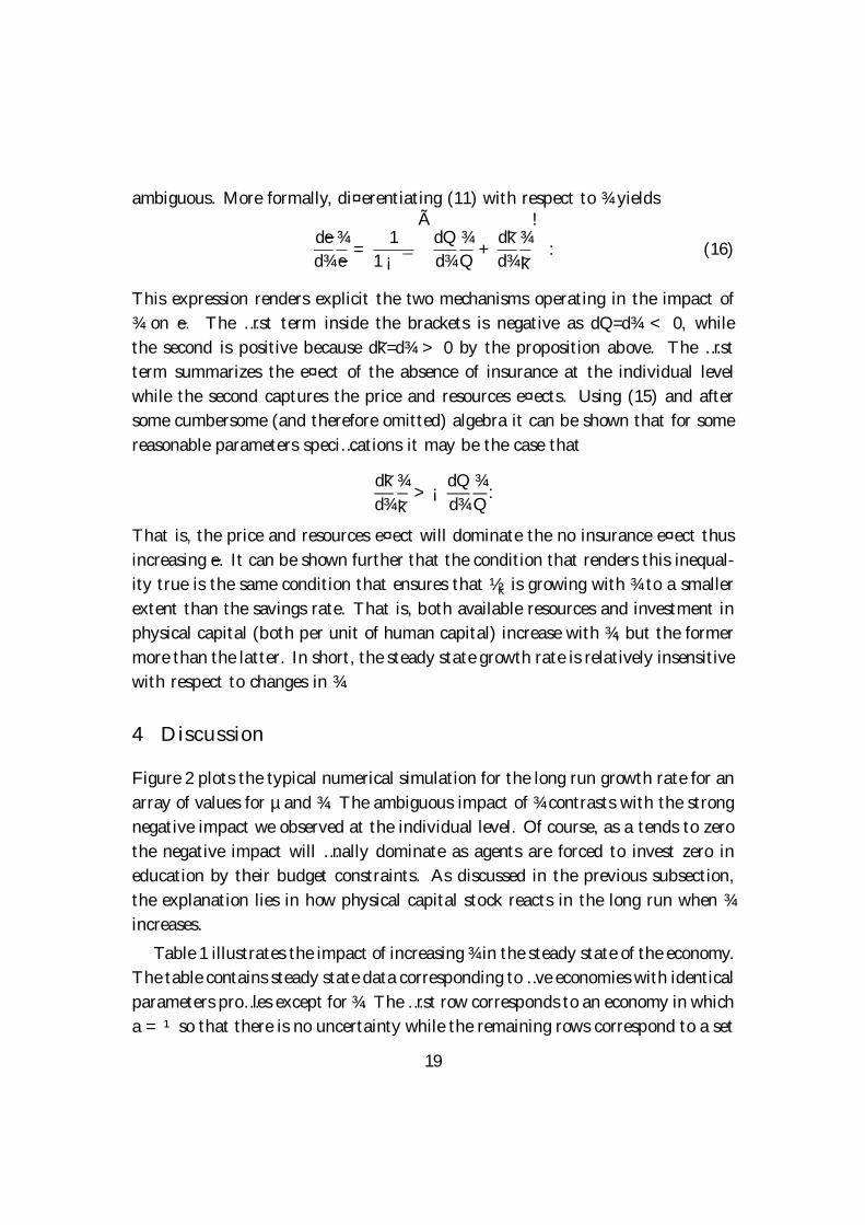
Figure 2 plots the typical numerical simulation for the long run growth rate for anarray of values for µ and ¾. The ambiguous impact of ¾ contrasts with the strongnegative impact we observed at the individual level. Of course, as a tends to zerothe negative impact will …nally dominate as agents are forced to invest zero ineducation by their budget constraints. As discussed in the previous subsection,the explanation lies in how physical capital stock reacts in the long run when ¾

increases.

Table 1 illustrates the impact of increasing ¾ in the steady state of the economy.The table contains steady state data corresponding to …ve economies with identicalparameters pro…les except for ¾. The …rst row corresponds to an economy in whicha = ¹ so that there is no uncertainty while the remaining rows correspond to a set

19

Figure 2. The impact of no insurance in the long run

of economies in which a decreases (¹ constant) until a is 25% of the average shock.We have chosen an example in which the growth rate is relatively insensitive tochanges in ¾ until the point in which the growth rate would start to decrease byfeasibility.

A decrease of a from 100% to 25% causes the growth factor to slightly increase…rst from 2.25 to 2.26 and then decrease to 2.24. If each period is interpreted torepresent 30 years, these changes amount to variations between 2.72% and 2.76%in terms of annual growth rates. The changes are close to irrelevant.

Above we identi…ed two mechanisms by which the negative impact of ¾ atthe individual level could be compensated. The price e¤ect is related to humancapital becoming relatively more scarce. The ratio of physical to human capitalsharply increases causing wages to and the interest factor to increase and de-crease respectively. The wage increases 5.1% with respect to the no uncertaintyeconomy while the interest factor falls from 29.22 (11.9% annual rate) to 26.9(11.6% annual rate). The second (positive) e¤ect compensating the negative im-pact of ¾ at the individual level is that of resources. Observe that the share ofeducation in savings ~½k decreases by 10%. Nevertheless, the savings rate of theeconomy sharply increases from 3.9% to 4.5% thus compensating the reduction ininvestment in human capital. As a consequence, the share of education in output

20

a=¹ ¹~e¯ ~k 1 + ~r ~w St=Yt Et+1=St Et+1=Yt

100% 2.25 0.014 29.22 0.98 0.0392 0.4118 0.0161

75% 2.25 0.014 28.52 0.99 0.0397 0.4043 0.0161

50% 2.26 0.016 26.29 1.03 0.0414 0.3782 0.0157

25% 2.24 0.022 21.61 1.12 0.0452 0.3113 0.0141

Table 1. The e¤ect of increasing ¾ in the steady state

steadily decreases from 1.6% to 1.4% even when the growth rate increases: thesecond economy grows at a factor 2.25 with share 1.61% while the third economygrows faster 2.26 with share 1.57%.

To end this section let us point out that ¾ has an obvious e¤ect in terms ofinequality. The absence of insurance a¤ects the same way all agents ex ante butnot ex post. Once the productivity shock is realized all agents face the same debt(1 + rt+1)et but di¤erent labor earnings ztwte

¯t so that the distribution of zt will

determine the shape of the earnings distribution. Of course, higher values of ¾

will be associated with higher degrees of inequality in relative terms. Figure 3plots the Lorenz curves net labor earnings for …ve economies that only di¤er in¾. For a given level of ¹ we consider a to be from 90% to 10% of the averageshock. The lower is a the more unequal the distribution of (net) earnings will be.Since we have chosen agents to have homogeneous preferences, the savings rate isthe same for all levels of earnings so that the distribution of wealth will displayidentical characteristics as that of earnings.

5 Conclusions

In this paper we have analyzed a general equilibrium model of investment ineducation when the returns to this investment are uncertain and agent cannotinsure themselves. Con…rming previous partial equilibrium analyses, at the indi-vidual level the impact of uncertainty is negative and very strong. Nevertheless,at the aggregate other mechanisms will operate to compensate the initial individ-ual incentive to reduce investment in education. As a consequence, our economydescribes a world in which very di¤erent degrees of uncertainty can yield similarlong run growth rates. This result warns us about the usual interpretation of the

21

Figure 3. Lorenz curves for increasing µ

role of human capital as an engine for growth.

It is commonly accepted that the accumulation of human capital is at least oneof the characteristics that allow modern market economies to grow sustainably.What we show is that the relationship or the mechanisms by which human capitalinduce growth may be subtle. When we model education as investment of realresources, rather than schooling, education causes growth but growth also causeseducation: making resources available that will eventually be devoted to educationin the future. Actual economies, however, may be growing at similar rates andnevertheless display di¤erent intensities of human capital, shares of investment ineducation, degrees of inequality, or savings rates.

Our model describes a world in which economies can grow at the same ratebut displaying signi…cantly di¤erent structures. A model economy with a highdegree of uncertainty (high variance of the shock) can grow at the same rate asan economy with low uncertainty but be more physical capital intensive, in termsof the share of physical capital investment in savings, and display large degreesof inequality. In contrast, model economies with low degrees of uncertainty havehigher levels of output, are human capital intensive, and display lower levels ofinequality. Such picture roughly describes what we observe in a world in which

22

developing countries grow at the same rate as developed countries but with thecharacteristics of a model economy with a high degree of uncertainty: low levelsof human capital, less investment in education in relative terms, and large degreesof inequality.

These results suggest that unequal opportunities to access to education, dueto …nancial restrictions, a¤ect more the distribution of earnings rather than thelong run performance of the economy. In terms of economic policy, they suggestthat policies of public education should in the …rst place be conceived as a meanto smooth inequality, rather than to foster growth.

6 References

Aghion, P. and Bolton, P. (1992) “Distribution and growth in models of imperfectcapital markets,” European Economic Review, 36, 603-611.

Altonji, J.G. and T.A. Dunn (1996) “The e¤ects of family characteristics on thereturn to education,” Review of Economics and Statistics, 78, 692–704.

Becker, G.S. (1962) “Investment in human capital: A theoretical analysis,” Jour-nal of Political Economy, 70, 9–49.

Becker, G.S. (1975) Human capital: A theoretical and empirical analysis withspecial reference to education. Columbia University Press.

Card, D. and A.B. Krueger (1992) “Does school quality matter? Returns toeducation and the characteristics of public schools in the United States,”Journal of Political Economy, 100, 1–40.

Galor, O. and Zeira, J. (1993) “Income distribution and macroeconomics,” Reviewof Economic Studies, 60, 35-52.

Kodde, D.A. (1986) “Uncertainty and the demand for education,” Review of Eco-nomics and Statistics, 68, 460-467.

Kodde, D.A. and J.M.M. Ritzen (1985) “The demand for education under capitalmarket imperfections,” European Economic Review, 28, 347-362.

Levhari, D. and Y. Weiss (1974) “The e¤ect of risk on the investment in humancapital,” American Economic Review, 64(6), 950–963.

Lucas, Jr., R.E. (1988) “On the mechanics of economic development,” Journal ofMonetary Economics, 22, 3-42.

Michel, P. (1993) “Le modèle à générations imbriquées, un instrument d’analyse

23

macroéconomique,” Revue d’Economie Politique, 103, 191–220.

Schultz, T.W. (1960) “Capital formation by education,” Journal of Political Econ-omy, 69, 571–583.

Schultz, T.W. (1961) “Investment in human capital,” American Economic Review,51(1), 1–17.

Snow, A. and R.S. Warren (1990) “Human capital investment and labor supplyunder uncertainty,” International Economic Review, 195-205.

Stokey, N. (1998) “Shirtsleeves to shirtsleeves: the economics of social mobil-ity,” in Ehud Kalai (ed.) Collected Volume of Nancy L. Schwartz Lectures.Cambridge University Press.

U.S. Congress (2000) “Investment in education: Private and public returns,” JointEconomic Committee, Vice Chairman Jim Saxton (R-NJ), January.

Williams, J.T. (1978) “Risk, human capital, and the investor’s portfolio,” Journalof Business, 51(1), 65-89.

Williams, J.T. (1979) “Uncertainty and the accumulation of human capital overthe life cycle,” Journal of Business, 52(4), 521-548.

24