MontréalFévrier 2002

Série ScientifiqueScientific Series

2002s-11

Idiosyncratic ConsumptionRisk and the Cross-Section of

Asset ReturnsKris Jacobs, Kevin Q. Wang

CIRANO

Le CIRANO est un organisme sans but lucratif constitué en vertu de la Loi des compagnies du Québec. Lefinancement de son infrastructure et de ses activités de recherche provient des cotisations de ses organisations-membres, d’une subvention d’infrastructure du ministère de la Recherche, de la Science et de la Technologie, demême que des subventions et mandats obtenus par ses équipes de recherche.

CIRANO is a private non-profit organization incorporated under the Québec Companies Act. Its infrastructure andresearch activities are funded through fees paid by member organizations, an infrastructure grant from theMinistère de la Recherche, de la Science et de la Technologie, and grants and research mandates obtained by itsresearch teams.

Les organisations-partenaires / The Partner Organizations

•École des Hautes Études Commerciales•École Polytechnique de Montréal•Université Concordia•Université de Montréal•Université du Québec à Montréal•Université Laval•Université McGill•Ministère des Finances du Québec•MRST•Alcan inc.•AXA Canada•Banque du Canada•Banque Laurentienne du Canada•Banque Nationale du Canada•Banque Royale du Canada•Bell Canada•Bombardier•Bourse de Montréal•Développement des ressources humaines Canada (DRHC)•Fédération des caisses Desjardins du Québec•Hydro-Québec•Industrie Canada•Pratt & Whitney Canada Inc.•Raymond Chabot Grant Thornton•Ville de Montréal

© 2002 Kris Jacobs et Kevin Q. Wang. Tous droits réservés. All rights reserved. Reproduction partielle permiseavec citation du document source, incluant la notice ©.Short sections may be quoted without explicit permission, if full credit, including © notice, is given to the source.

ISSN 1198-8177

Les cahiers de la série scientifique (CS) visent à rendre accessibles des résultats de recherche effectuée auCIRANO afin de susciter échanges et commentaires. Ces cahiers sont écrits dans le style des publicationsscientifiques. Les idées et les opinions émises sont sous l’unique responsabilité des auteurs et ne représententpas nécessairement les positions du CIRANO ou de ses partenaires.This paper presents research carried out at CIRANO and aims at encouraging discussion and comment. Theobservations and viewpoints expressed are the sole responsibility of the authors. They do not necessarilyrepresent positions of CIRANO or its partners.

Idiosyncratic Consumption Riskand the Cross-Section of Asset Returns*

Kris Jacobs† and Kevin Q. Wang‡

First version: Novembre 2000This revision: August 2001

Résumé / Abstract

Cet article analyse l’importance du risque idiosyncratique de la consommation individuelle pour lavariance transversale des rendements moyens des actifs et des obligations. Lorsque l’on n’attribue pas deprix au risque idiosyncratique de la consommation individuelle, le seul facteur d’évaluation dans uneéconomie à plusieurs horizons est le taux de croissance de la consommation agrégée. Nous montrons quela variance transversale de la croissance de la consommation est également un facteur dont le prix estdéterminé. Ceci démontre que les consommateurs ne sont pas complètement assurés contre le risqueidiosyncratique de la consommation et que les rendements des actifs reflètent leurs efforts à réduire leurexposition à ce risque. Pour la période considérée, nous trouvons que le modèle d’évaluation d’actifs àdeux facteurs basés sur la consommation donne de meilleurs résultats que le CAPM. De plus, laperformance empirique du modèle se compare favorablement avec celle du modèle à trois facteurs deFama-French. Par ailleurs, en présence du facteur de marché et des facteurs taille et ratio valeurcomptable/cours, les deux facteurs basés sur la consommation conservent leur pouvoir explicatif.Combiné aux résultats de Lettau et Ludvigson (2000), ces résultats indiquent que l’évaluation d’actifs àpartir de la consommation sert à expliquer l’intégralité des rendements d’actifs.

This paper investigates the importance of idiosyncratic consumption risk for the cross-sectionalvariation in average returns on stocks and bonds. If idiosyncratic consumption risk is not priced, the onlypricing factor in a multiperiod economy is the rate of aggregate consumption growth. We offer evidencethat the cross-sectional variance of consumption growth is also a priced factor. This demonstrates thatconsumers are not fully insured against idiosyncratic consumption risk, and that asset returns reflect theirattempts to reduce their exposure to this risk. We find that over the sample period the resulting two-factorconsumption-based asset pricing model significantly outperforms the CAPM. The model’s empiricalperformance also compares favorably with that of the Fama-French three-factor model. Moreover, in thepresence of the market factor and the size and book-to-market factors, the two consumption based factorsretain explanatory power. Together with the results of Lettau and Ludvigson (2000), these findingsindicate that consumption-based asset pricing is relevant for explaining the cross-section of asset returns.

JEL: G12

Mots clés : évaluation d’actifs transversale, modèle basé sur la consommation, risque de consommationidiosyncratique, marchés incomplets, erreur de mesure

Keywords: cross-sectional asset pricing; consumption-based model; idiosyncratic consumption risk;incomplete markets; measurement error

* Jacobs acknowledges FCAR of Québec and SSHRC of Canada for financial support. Wang acknowledges the Connaught Fundat the University of Toronto for financial support. We are very grateful to Eugene Fama and Raymond Kan for providing us withthe asset return data. We would also like to thank Joao Cocco, Francisco Gomes, Raymond Kan, Tom McCurdy, SergeiSarkissian and Raman Uppal for helpful comments. Correspondence to: Kris Jacobs, Faculty of Management, McGill University,1001 Sherbrooke Street West, Montreal, Canada H3A 1G5; Tel: (514) 398-4025; Fax: (514) 398-3876; E-mail:Jacobs@Management.McGill.CA.† Jacobs: Assistant Professor of Finance, Faculty of Management, McGill University and fellow CIRANO.‡ Wang: Assistant Professor of Finance, Joseph L. Rotman School of Management, University of Toronto.

1 Introduction

If agents manage to perfectly insure themselves against idiosyncratic consumption risk, theonly relevant pricing factor in a standard multiperiod asset pricing model without frictionsis the growth rate of aggregate consumption. However, the workhorse representative-agentconsumption-based asset pricing model (CCAPM) that reßects this allocation is not ableto match important aspects of the distribution of historical asset returns, such as the riskpremium on the market portfolio. Its performance in a cross-sectional context is weak andhas certainly not been sufficiently satisfactory to threaten alternative cross-sectional modelssuch as the Capital Asset Pricing Model (CAPM).1

However, if agents cannot perfectly insure themselves against idiosyncratic consumptionrisk,2 factors other than aggregate consumption growth become relevant to price assets. Un-der this assumption, all higher moments of the cross-sectional distribution of consumptiongrowth are relevant pricing factors. Researchers have long realized that changes in thesemoments may be of critical importance to explain changes in asset prices (see Mehra andPrescott (1985)). Building on this insight, a number of studies have investigated the impor-tance of market incompleteness for the equity premium puzzle and the risk-free rate puzzle(see Telmer (1993), Constantinides and Duffie (1996), Heaton and Lucas (1996), Jacobs(1999), Vissing-Jorgensen (2000), Cogley (1999), Brav, Constantinides and Geczy (1999)and Balduzzi and Yao (2000)). These studies provide mixed evidence on market incomplete-ness and the literature has not yet fully matured, but it is a safe conclusion that modelswith uninsurable idiosyncratic consumption risk and potentially limited market participationstand a better chance to explain the data than standard representative-agent models.This paper further investigates the importance of uninsurable idiosyncratic risk by ex-

amining its importance for the cross-section of asset returns. In principle, one can investi-gate the set of intertemporal restrictions associated with the cross-section of returns usinga number of alternative procedures. For instance, one can specify a utility function anduse a distributional assumption to obtain a pricing kernel that is a well-deÞned nonlinearparametric transformation of consumption-based pricing factors. Constantinides and Duffie(1996) use such a setup with constant relative risk aversion and a lognormality assumptionon idiosyncratic income shocks. They obtain two consumption-based pricing factors, rep-

1A recent paper by Lettau and Ludvigson (2000) demonstrates that consumption-based models canchallenge the CAPM along certain dimensions. This research is discussed below.

2At this point, it is important to elaborate on the terminology used in this paper in order to avoidconfusion. In the literature on the CAPM, standard terminology splits up the risk of an individual assetinto market risk and idiosyncratic risk. In this paper the focus is on idiosyncratic risk for an individualconsumer. It is standard in the incomplete markets literature to refer to this risk as “idiosyncratic incomerisk or “idiosyncratic risk. In this paper we do not investigate a full general equilibrium model but focusexclusively on equilibrium intertemporal consumption allocations. Therefore we refer to this idiosyncraticrisk as “idiosyncratic consumption risk. This terminology is slightly unsatisfactory but preferable to theuse of “idiosyncratic risk, which could be confused with the terminology used in the context of the CAPM.

2

resenting the rate of consumption growth and the cross-sectional variance of the logarithmof consumption growth (consumption dispersion). Alternatively, Cogleys (1999) analysisillustrates the importance of additional pricing factors representing higher moments of thecross-sectional distribution of consumption growth. We follow a slightly different approach,designed to keep the econometric analysis relatively simple and to allow us to conduct asearch over different speciÞcations. To do this, we investigate a variety of pricing kernelsthat are linear in consumption growth and consumption dispersion.We investigate the empirical performance of these pricing kernels using household con-

sumption data from the Consumer Expenditure Survey (CEX). We examine the performanceof the pricing kernels using four different datasets. The Þrst two datasets use data on non-durables and services consumption. The difference between the two samples is that theÞrst dataset is based on all households that fulÞll certain selection criteria, whereas the sec-ond dataset only contains households that hold assets. The difference between the thirdand the fourth dataset is also based on whether the household holds assets, but both thesedatasets use data on total consumption. Moreover, for each of the resulting four datasets,we construct the consumption-based pricing factors in different ways. First, we computeaverage consumption growth and consumption dispersion by using data on individual house-hold consumption. However, we know that the presence of measurement error is a seriousproblem when using household consumption data. To deal with this problem, we recon-struct the consumption-based factors using data on the consumption of a synthetic cohortof individuals, rather than a single individual.We Þnd that regardless of the dataset, consumption dispersion is a priced factor, in-

dicating the relevance of uninsurable consumption risk for asset returns. The sign of thepriced consumption dispersion factor depends on the dataset. This is of interest because foridiosyncratic consumption risk to help resolve the equity premium puzzle, it has to be thecase that consumption dispersion is larger in recessions. Intuitively this leads to an increasein the risk faced by an individual agent, and this leads to a larger risk premium to induceinvestors to hold risky assets. However, we Þnd that whereas the Þrst consumption-basedfactor (average consumption growth) always displays the expected positive correlation withreturns, we only obtain robust estimates of negative correlation between returns and con-sumption dispersion when considering data on total consumption, and only when limitingthe sample to asset holders.This Þnding is not surprising. Other studies also conclude that the distribution of

consumption for assetholders is different from that for non-assetholders. Moreover, durableconsumption is the most cyclical component of individual consumption. Therefore, the datasimply tell us that the less wealthy cut back a lot more than the wealthy on their consumptionin recessions and make up for it in expansions. However, because it is relatively harder tocut back on nondurable consumption, they implement this through their expenditures ondurable consumption. Finally, it must be noted that these Þndings are obtained usingpricing factors constructed from cohort data. When using individual data, estimates are

3

often insigniÞcant and not very robust. This Þnding is consistent with the Þndings of Brav,Constantinides and Geczy (1999) in the context of the equity premium puzzle.To evaluate the signiÞcance of these Þndings, we investigate their robustness and compare

the performance of the pricing factors against a number of alternatives. We Þnd that thetwo-factor consumption-based model (with consumption growth and consumption dispersionas factors) signiÞcantly outperforms the CAPM and the one-factor consumption based modelover the sample period under consideration. Moreover, the empirical performance of thetwo-factor consumption-based model also compares favorably with that of the three-factormodel proposed by Fama and French (1993). Finally, we investigate pricing kernels thatcombine size and book-to-market factors and/or the CAPM factor with the consumption-based factors. It is shown that even after accounting for these alternative pricing factors,the consumption-based factors are estimated signiÞcantly in the pricing equation.

2 Idiosyncratic Consumption Risk and the Cross-Section

of Asset Returns

Following the seminal contributions by Lucas (1978) and Breeden (1979), a number of pa-pers have conducted empirical investigations of representative-agent consumption-based as-set pricing models. Even though these models have a wide range of empirical implications, alarge part of the literature has a rather limited focus. In fact, much of the empirical researchon consumption-based models has focused exclusively on the returns on a riskless asset andthe market index, leading to the so-called equity premium and riskfree rate puzzles.3 Asmall number of papers study the performance of the consumption-based model in a cross-sectional context. Mankiw and Shapiro (1986), Breeden, Gibbons and Litzenberger (1989)and Cochrane (1996) conclude that the performance of the consumption-based model is un-satisfactory and that the consumption-based model performs no better than the CAPM.However, more recently Lettau and Ludvigson (2000) show that those negative conclusionsabout the performance of the consumption-based model are due to the fact that those em-pirical studies investigate an unconditional linear factor model. When investigating a con-ditional factor model, the models performance is about as good as that of the three-factorFama-French model, when using a speciÞc conditioning variable that is suggested by theory.Campbell and Cochrane (2000) provide an explanation for why consumption-based assetpricing models perform better conditionally than unconditionally.This paper reaffirms that consumption-based asset pricing models are valuable for the

study of the cross-section of asset returns. It shows that this is the case even when studying

3Hansen and Singleton (1982,1984), Mehra and Prescott (1985) and Grossman, Melino and Shiller (1985)focus exclusively on a riskless and a risky asset. Other papers such as Hansen and Singleton (1983) andEpstein and Zin (1991) focus on the equity premium puzzle but investigate some other risky assets. However,none of these papers speciÞcally focuses on the cross-section of returns.

4

unconditional models, as opposed to the conditional models studied by Lettau and Ludvigson(2000). The key to this Þnding is that one has to move away from the rigid construction ofa representative agent economy, which implies the irrelevance of idiosyncratic consumptionrisk. To appreciate the importance of this modeling approach, it is instructive to reviewthe importance of complete markets and the representative agent assumption for the equitypremium and riskfree rate puzzles.4 The complete markets assumption is critical for the rep-resentative agent model. Individual agents that are faced with a complete markets structurecan insure themselves against idiosyncratic consumption risk. As a consequence, the pricesof assets in the economy are equivalent to the prices in a closely related representative agenteconomy.Whereas the complete markets assumption is a convenient modeling technique, casual

observation as well as empirical testing has convinced most researchers that it is not veryrealistic (see Cochrane (1991), Mace (1991), Hayashi, Altonji and Kotlikoff (1994)). It istherefore not surprising that a growing number of studies investigate to what extent marketincompleteness is of interest to explain the empirical rejections of the consumption-basedmodels. A number of these studies investigate this issue by using simulation-based models.Whereas early studies by Telmer (1993) and Heaton and Lucas (1996) do not manage togenerate large enough risk premia for most realistic parameterizations of the economy, laterstudies by Telmer, Storesletten and Yaron (1997) and Constantinides, Donaldson and Mehra(1998) have managed to generate larger risk premia under the assumption that idiosyncraticshocks are fairly persistent. A number of other studies (Jacobs (1999), Vissing-Jorgensen(2000), Cogley (1999), Brav, Constantinides and Geczy (1999) and Balduzzi and Yao (2000))have analyzed market incompleteness from another perspective, by investigating Euler equa-tions that hold even if markets are incomplete. Sarkissian (1998) analyzes incomplete risksharing between countries. The test results in these papers are mixed, but a robust con-clusion is that risk aversion implied by restrictions from incomplete markets is lower thanrisk aversion implied by representative agent models. Taken together, the Þndings in theliterature on market incompleteness seem to indicate that accounting for idiosyncratic con-sumption risk has at least some potential to explain the structure of asset returns.Because models with incomplete markets have had some success explaining the equity

premium and risk-free rate puzzles, it seems therefore natural to investigate if they can

4The literature contains other attempts to explain the equity premium puzzle and riskfree rate puzzle.A number of papers have focused on the importance of time aggregation (see Grossman, Melino and Shiller(1987) and Heaton (1993)). Also, an extensive literature has studied the modeling of alternative preferencesfor the representative agent (see Abel (1990), Campbell and Cochrane (1999), Cochrane and Hansen (1992),Constantinides (1990), Detemple and Zapatero (1990), Epstein and Zin (1991), Ferson and Constantinides(1991), Heaton (1995), and Sundaresan (1989)) . These approaches alleviate some of the problems withrepresentative agent models and it is possible that they would also improve the cross-sectional performanceof consumption-based models. See Kocherlakota (1996), Campbell, Lo and MacKinlay (1997) and Cochrane(2001) for overviews of this literature.

5

be used to explain a wider cross-section of asset returns. In cross-sectional asset pricing,the Capital Asset Pricing Model (CAPM) is the dominant paradigm. It is therefore anatural benchmark to evaluate the performance of a consumption-based model with marketincompleteness. Ferson (1995) and Cochrane (1996, 2001) show that the traditional formof factor pricing models such as the CAPM can be implemented by using the intertemporaloptimality condition

E[MtRj,t|Ωt−1] = 1 (1)

where Mt is the pricing kernel, Rj,t is the return on asset j at time t and Ωt−1 is theinformation set available to the econometrician at time t − 1. For the CAPM, the pricingkernel Mt is speciÞed as follows

Mt = β0 + β1RM,t (2)

where RM,t is the return on the market portfolio at time t. We now outline a frameworkthat allows us to compare the performance of a pricing kernel that accounts for idiosyncraticconsumption risk with the performance of the CAPM as evaluated in (1) and (2). Theintertemporal optimality condition associated with individual is investment in asset j impliesthat

E[Mi,t(cgi,t)Rj,t|Ωt−1] = 1 (3)

where the pricing kernelMi,t which is indexed by individual i depends on consumption growthcgi,t = ci,t/ci,t−1 in the context of a consumption-based asset pricing model. Averaging thisorthogonality condition for asset j over all N consumers we get

E[(1/N)NXi=1

Mi,t(cgi,t)Rj,t|Ωt−1] = 1 (4)

The pricing kernel in (4) will also be referred to as Mt = (1/N)PNi=1Mi,t(cgi,t). Eval-

uating the performance of this kernel in the cross-section can then be accomplished byspecifying the underlying structure of the economy. For instance, if individual consumershave time-separable constant relative risk aversion (TS-CRRA), this average intertemporalEuler equation for consumer i and asset j is

E[(1/N) e−θNXi=1

(cgi,t)−αRj,t|Ωt−1] = 1 (5)

where α is the rate of relative risk aversion and θ is the rate of time preference.Constantinides and Duffie (1996, henceforth CD) clearly highlight the importance of

consumption dispersion under market incompleteness. Using a TS-CRRA speciÞcation, theyspecify an economy that leads to an Euler equation that speciÞes explicitly how the pricing

6

kernel depends on the moments of the cross-sectional distribution of consumption growth.SpeciÞcally, their economy yields the following intertemporal Euler equation

E[e−θ(ct/ct−1)−α exp(

α(α+ 1)

2y2t )Rj,t|Ωt−1] = 1 (6)

where ct is aggregate consumption at time t and y2t can be interpreted as the variance of

the cross-sectional distribution of log[(ci,t/ct)/(ci,t−1/ct−1)].5 Cogley (1999) uses a different

approach to show that in general the pricing kernel will depend on all moments of thecross-sectional distribution. When omitting moments higher than the second moment andspecializing the analysis to a TS-CRRA utility function, he shows that one obtains an Eulerequation similar to (6).The cross-section of asset returns can be analyzed by using the generalized method of

moments to evaluate (5) and (6) directly. However, the disadvantage of this approach is thatthe resulting econometric problem is highly nonlinear. This may complicate the optimizationand the comparison with the benchmark CAPM because of the existence of local optima.We therefore use a different approach inspired by Cochrane (1996). It is clear from Cogley(1999) that with incomplete markets the pricing kernel depends on the cross-sectional mo-ments of consumption growth.6 Moreover, because it is difficult to estimate higher momentsprecisely, it is preferable to limit attention to the Þrst two moments. The precise nature ofthe relationship between the pricing kernel and these moments depends on the speciÞcationof the utility function. We therefore assume that the pricing kernel depends in a simplelinear way on the Þrst two cross-sectional moments of consumption growth7

Mt = β0 + β1mcgt + β2vcgt (7)

where mcgt = (1/N)PNi=1(cgi,t) and vcgt = (1/N)

PNi=1(cgi,t −mcgt)2. Implicitly of course

this linear kernel corresponds to some utility function. If this utility function is a poorapproximation of reality, this will affect the performance of the pricing kernel negatively.8

5Balduzzi and Yao (2000) use a different setup which leads to a different Euler equation. In their economythe second factor is not the cross-sectional variance of log consumption growth, but the difference of thevariance in cross-sectional consumption. They also use this kernel to study the cross-section of asset returns.

6It must be noted that market incompleteness is not a necessary condition for the higher moments ofconsumption growth to enter the pricing kernel. For example, investor heterogeneity can have similareffects (Dumas (1989)). Basak and Cuoco (1989) explicitly characterize the cross-sectional distribution ofconsumption in a model with market incompleteness and investor heterogeneity.

7Heaton and Lucas (2000) also investigate linear pricing kernels with measures of idiosyncratic incomerisk as pricing factors. They Þnd that the existence of entrepreneurial income risk has a signiÞcant inßuenceon asset returns.

8Notice however that the linear kernel can be seen as a Taylor series approximation to any utility functionas long as one does not impose restrictions emanating from an underlying utility function on the coefficientsin (7).

7

We also compare the performance of the consumption-based factors to a benchmark otherthan the CAPM. A logical choice is to make a comparison with the size and book-to-marketfactors proposed by Fama and French (1992, 1993). We use the kernel for the Fama-Frenchthree factor model

Mt = β0 + β1RM,t + β2SMBt + β3HMLt (8)

where SMBt is the size factor and HMLt is the book-to-market factor. To evaluate therelative performance of the consumption-based factors compared to the Fama-French factors,we investigate a number of kernels where we interact the consumption-based factors withthe size and/or book-to-market and/or market factors. These kernels are described in moredetail in the tables.

3 Data Description

This section discusses three different issues related to data construction. The empiricalprocedure is implemented as follows. First, consumption data are used to construct pricingfactors that estimate the Þrst and the second moments of the cross-sectional distribution ofconsumption growth. The approach used to construct the consumption data is described inSection 3.2. In a second stage, these pricing factors are taken as given in an econometricinvestigation of the intertemporal relation (1) for a wide cross-section of asset returns. Thiscross-section of asset returns is described in Section 3.1. It must be noted at this point thatthe uncertainty involved in constructing the pricing factors is neglected in this econometricanalysis. A Þnal critical issue related to data construction is the construction of syntheticcohorts described in Section 3.3. The motivation for using synthetic cohorts is the well-documented existence of substantial measurement error in household consumption data.Finally, Section 3.4 discusses at length the statistical properties of the four different samplesused in the analysis and the factors used in the pricing equation.

3.1 Asset Return Data

We use a set of test portfolios that includes the twenty-Þve size and book-to-market portfoliosof Fama and French (1993), a long term government bond, a long term corporate bond, andthe 3-month Treasury bill rate. The data are quarterly, and they are constructed from thecorresponding monthly data, ranging from April 1984 to December 1995. The Fama-Frenchportfolios are now widely used. They are value-weighted portfolios of stocks listed on theNYSE, AMEX, and NASDAQ. These portfolios are sorted on Þrm size and book-to-marketequity and exhibit strong cross-sectional dispersion in average returns. (For more details onthe portfolios, see Fama and French (1993)). For the bond returns, we use the total returnon Treasury bonds (the CRSP variable GBTRET), the total return on long term corporatebonds (the CRSP variable CBTRET), and the three-month T-bill rate. For the market

8

portfolio, we use the CRSP value-weighted portfolio of stocks listed on NYSE, AMEX, andNASDAQ that Fama and French use to proxy for the market portfolio.9 Also included in ourempirical tests are the size (SMB) and book-to-market (HML) factors of Fama and French.All the variables are in real terms.Descriptive statistics for the test portfolios are given in Table I. An important observation

is that for the stock portfolios, which are sorted according to size and book-to-market, thepattern of average returns is very different from the one documented in Fama and French(1993). This difference is due to the different sample period. Most importantly, for thesample under consideration in this paper, Table I conÞrms the observation of Cochrane(2001, p. 438) that the size effect has disappeared in the eighties.

3.2 Consumption Data

To construct the pricing factors, we use data on household consumption from the ConsumerExpenditure Survey (CEX). The CEX data have been used by a number of researchersto analyze the importance of idiosyncratic consumption risk for the equity premium puzzle(e.g. see Brav, Constantinides and Geczy (1999), Vissing-Jorgensen (2000), Cogley (1999)and Balduzzi and Yao (2000)). Balduzzi and Yao (2000) also present an analysis of cross-sectional pricing using their (different) pricing kernel. The advantage of the CEX is that itprovides a measure of total consumption, unlike other datasets such as the Panel Study ofIncome Dynamics. The CEX is not a genuine panel dataset, but a series of cross-sectionswith a limited time dimension. However, in the context of the exercise proposed in thispaper, this is not necessarily a very serious problem, because at each time we simply useevery available cross-section to construct cross-sectional moments.We construct the pricing factors using two measures of household consumption. The Þrst

measure corresponds to nondurable consumption plus services. The second measure corre-sponds to total consumption, including durable consumption. The use of data on durableconsumption is fairly common in the consumption literature, and its importance is well rec-ognized because durable consumption has different stochastic properties from nondurableconsumption (e.g. see Christiano, Eichenbaum and Marshall (1991), Darby (1975), Eichen-baum and Hansen (1990), Mankiw (1985), Ogaki and Reinhart (1998), Sargent (1978) andStartz (1989)). However, the modeling of durable consumption in this paper is nonstandard,largely because of data constraints. In the time-series literature on durable consumption,the starting point is a time series of the stock of durable goods. Consumption of durable

9We follow a long tradition in the Þnance literature by measuring RM,t using the return on publiclylisted stocks. A large number of studies have debated whether to include the return on human capital inthis construction (see Mayers (1972), Roll (1977), Fama and Schwert (1977), Campbell (1996), Jagannathanand Wang (1996) and Lettau and Ludvigson (2000)). We do not analyze this issue, because our primarymotivation for studying the CAPM here is to Þnd an appropriate benchmark for the performance of ourconsumption-based model, and not the appropriate speciÞcation of the market return.

9

goods is then usually modeled as a distributed lag in this stock variable. Because studiesbased on household data are based on reports on expenditures instead of a stock of durablegoods, we proceed in a different way. Hayashi (1985) models durable consumption us-ing household data by specifying a distributed lag in expenditure on durable goods.10 Inthis paper, we model consumption of total expenditures, implicitly treating nondurable anddurable consumption as perfect substitutes. This approach is motivated by the need to offeralternatives to the CAPM that have a small number of factors. By modeling durable andnondurable consumption separately, one would introduce separate factors for each consump-tion category. By modeling consumption as a distributed lag of past expenditures, laggeddurable consumption growth would show up as an extra factor.11

Even though participants in the CEX are interviewed on a quarterly basis, one can inprinciple construct consumption data for different frequencies. After each quarter, par-ticipants are asked detailed questions about their consumption patterns in the past threemonths. It is possible to construct monthly consumption data from these interviews. How-ever, the resulting time series is fairly constant over a three-month period and then jumps toanother level (see also Vissing-Jorgensen (2000) on this issue). Therefore, we follow most ofthe available literature that uses the CEX and construct quarterly data (see Brav, Constan-tinides and Geczy (1999), Vissing-Jorgensen (2000) and Cogley (1999)). The CEX data areavailable from 1984 to 1995. Because we use data on consumption growth, the Þrst availablequarter is therefore the second quarter of 1984. Also, because of a data matching problem,we cannot use data on the Þrst quarter of 1986. Moreover, several indicators revealed lowdata quality for the last quarter available (the fourth quarter of 1995). We therefore excludethis quarter. This leaves us with 45 quarterly observations.Another issue that deserves discussion is family composition. The CEX reports con-

sumption for the household unit. This complicates the analysis, because as a result oneof the factors driving cross-sectional and time-series differences in consumption is changesand differences in family size. There are several ways to correct for this when estimatingintertemporal optimality conditions in the presence of idiosyncratic consumption risk. First,one can include a function of family size in the deÞnition of consumption in period t. Thisis useful when directly analyzing the Euler equation (5) (see Jacobs (1999)). An secondalternative is to simply divide household consumption by the number of members of thehousehold. Whereas this is of course done when using aggregate per capita consumption

10The use of expenditure data is problematic to the extent that large expenditures are made at one pointin time on durable goods that yield consumption services at some other point in time. It must be notedin this respect that to the extent that consumers purchase durable goods on credit, the match betweenexpenditure and consumption is probably rather good.

11It is clear that because of data constraints the modeling of durable goods consumption is subject todifferent problems than the ones we encounter when using time-series data. If as a result of this the linkbetween the resulting pricing factors in (7) and the consumers utility function is unconvincing, one can alsointerpret the factors as attempting to capture business cycles in expenditures by consumers.

10

data, the issue is less straightforward when using household data because the data revealthat household consumption is a complicated nonlinear function of household size. A thirdalternative is to correct for family size using a given scale which is used in the literature orestimated from the data. The Þrst technique is not applicable in the context of this paper, be-cause we do not analyze the intertemporal optimality conditions directly. We Þrst constructthe factors and then use those factors in a regression framework. We attempted to correctfor household size using the second and third alternatives. Because this does not make adifference, we present results using household consumption as the unit of observation.A Þnal robustness issue is the presence of seasonalities. It is well known that season-

alities are present in consumption data and that they are important for asset pricing (seeMiron (1986) and Ferson and Harvey (1992)). When inspecting the raw CEX householdconsumption data, seasonalities seem to be even more pronounced than for quarterly NIPAdata. The most obvious manifestation of this Þnding is the well known dent in consump-tion in the Þrst quarter. Reported results do not adjust for seasonality, in accordance withother papers that use the CEX (see Attanasio and Weber (1995), Brav, Constantinides andGeczy (1999), Vissing-Jorgensen (2000), Cogley (1999) and Balduzzi and Yao (2000)). Weperformed a robustness exercise by controlling for seasonality using the census X11 methodas implemented in EVIEWS. Even though the resulting seasonal adjustment factors arenonnegligible (as is the case for NIPA data), this does not affect test results.In the expanding literature that investigates the equity premium puzzle using disaggre-

gate data, one important conclusion is that asset market participation is of great importance.It seems that the consumption patterns of households that hold assets are more consistentwith economic theory. One of the strengths of the CEX is that it contains a wealth ofinformation on asset holdings. We therefore conduct our analysis for a sample that containsall households, but also for a sample that only contains assetholders. Given the wealth ofasset information in the CEX, several selection criteria can be used and existing studies haveconstructed widely different samples of assetholders. For example, the CEX reports dataon holdings of checking and savings accounts, bonds and stocks, and participation in privateand public pension plans. Moreover, the CEX reports data on the income received from acertain asset (a ßow variable) as well as the holdings of the same asset (a stock variable).Also, in the CEX all these questions are asked in reference to two points in time, the Þrstand the last (Þfth) quarter that the households are in the sample. To determine whichhouseholds are assetholders, we use the answer referring to the Þrst quarter.Ideally we would like to construct a sample of individuals who hold any type of asset and

also a sample of individuals who hold stocks. Unfortunately, this is not possible because theCEX does not ask a direct question on whether an individual holds stocks either directly orindirectly through a pension plan. We therefore proceed to construct a sample of householdswho are very likely to hold stocks. It consists of households that report the existence of atleast one of the following: (i) holdings of stocks or bonds, (ii) dividend income, and/or (iii)contributions to an IRA. It is clear that this is an imperfect measure of stock ownership.

11

However, in our opinion it is the best one can do with the CEX.A Þnal issue regarding the construction of this sample of assetholders is that we only con-

struct a sample of households who report positive holdings of assets. Interestingly, severalstudies (Mankiw and Zeldes (1991), Jacobs (1999), Brav, Constantinides and Geczy (1999),Vissing-Jorgensen (2000)) have constructed additional samples containing only householdswho report holdings above certain positive thresholds (e.g. $1,000, $5,000 etc.). We do notattempt to do this because of two reasons. First, unlike other papers we construct a sampleof assetholders using different questions. Therefore, imposing thresholds is less straightfor-ward. Second, our construction of synthetic cohorts described in the next section is onlymeaningful if the sample size is large enough. By eliminating more and more householdsdue to increasingly stringent asset holding criteria, this exercise becomes problematic.

3.3 Dealing with Measurement Error: Constructing Synthetic Co-horts

We start out by constructing pricing factors using the cross-section of individual consump-tion growth at every time t. This gives us time series of factors consisting of 45 observations.Subsequently, we use these pricing factors in a cross-sectional pricing relationship. Theproblem with this approach is the existence of measurement error in household consump-tion data, which is well documented (e.g., see Altonji (1986), Altonji and Siow (1987),and Zeldes (1989)). Several studies that use household consumption data to analyze as-set pricing relationships try to mitigate the inßuence of measurement error. For example,Vissing-Jorgensen (2000) uses log-linearized Euler equations because it is well-known thatmeasurement error can be more effectively dealt with in a linear framework. Mankiw andZeldes (1991) and Balduzzi and Yao (2000) construct time series of average household con-sumption using household data. This minimizes the impact of measurement error underplausible assumptions.One can argue that in our approach the effects of measurement error are less serious

because we do not analyze the nonlinear Euler equations. However, the potential problemwith measurement error still arises in the construction of the consumption-based pricingfactors. To deal with this problem, we adopt the synthetic cohorts approach which is pop-ular in the economics literature. This approach was previously used by (among others)Browning, Deaton and Irish (1985) and for the CEX data by Attanasio and Weber (1995).It basically involves the construction of a representative consumer for a typical group whichcan be deÞned by observable characteristics such as age. It is clear that for most plausibleparameterizations of measurement error this construction will mitigate its effects, withouteliminating them. It must also be noted that the motivation for this technique is of coursevery similar to the motivation for testing the CAPM using portfolios instead of individual as-sets, as originally implemented by Black, Jensen and Scholes (1972) and Fama and MacBeth

12

(1973).Unfortunately, the choice of grouping method for the construction of synthetic cohorts

is not obvious. On the one hand, one does not want the groups to be too small, because inthat case the effects of measurement error are not likely to disappear. On the other hand,by making the groups too large, it is clear that one constructs away the potential impact ofidiosyncratic consumption risk. It is not obvious that there is a realistic optimal solutionto this problem. The optimal choice depends on the size and the type of the measurementerror, and by deÞnition we do not know a lot about this. We choose to construct syntheticcohorts based on two very simple grouping variables, namely the age and the educationof the household head. To understand the problems implied by this choice, note thatfor all speciÞcations we work with two samples, one with all households and another withassetholders only. It is clear that the choice to hold assets or not critically depends on ageand education. Therefore, the composition and size of a given cohort will be different inboth samples, and this could inßuence test results. To minimize these (potential) problems,we impose a constraint on the cohort construction: we only include individuals older than 24and younger than 64 in the sample to increase the probability of having a sufficient numberof observations in each cohort.We then proceed to construct factors in the following two ways. The Þrst set of factors

is based on age only: a cohort consists of all households with a household head of a certainage. We are therefore constructing the pricing factors in each quarter using 39 observations(cohorts). A second construction uses age as well as education as a sorting variable. In theCEX, there are seven educational categories. We use this educational information to createa sample of consumers who have at least completed a college education, and another sampleof consumers who have not. This construction gives us a maximum of 78 (39× 2) cohortsin each time period to construct the pricing factors. However, in practice this number issometimes lower because we do not have observations on certain cohorts.The Þnal issue regarding cohort construction is what we choose to aggregate on within

the cohort. Whereas the object of interest is consumption growth, one can also computeconsumption growth after aggregating on the level of consumption. For certain types ofmeasurement error, this may actually be preferable. We therefore decide to report resultsusing both methods. We now turn to a complete description of the construction of thesefactors, using the different methods. We refer to the construction of factors using individualdata using a subscript 1, that is

mcg1,t = (1/N)NXi=1

(cgi,t) vcg1,t = (1/N)NXi=1

(cgi,t −mcg1,t)2

where cgi,t = (ci,t/ci,t−1) and ci,t is the consumption of individual i at time t.Now consider averaging over consumption growth to obtain the consumption growth

of a representative cohort j, cohcg2,j,t = (1/Nj,t)PNj,t

i=1 (cgi,t) where Nj,t is the number of

13

observations on this cohort at time t. With H the number of cohorts, the factors based onthis construction can then be computed as

mcg2,t = (1/H)HXj=1

(cohcg2,j,t) vcg2,t = (1/H)HXj=1

(cohcg2,j,t −mcg2,t)2

Alternatively, consider the consumption of a representative cohort k at time t, which is

given by cohck,t = (1/Nk,t)PNk,t

i=1 (ci,t). We then deÞne cohcg3,k,t = (cohck,t/cohck,t−1) andthe factors

mcg3,t = (1/H)HXk=1

(cohcg3,k,t) vcg3,t = (1/H)HXk=1

(cohcg3,k,t −mcg3,t)2

Summarizing, factors with a 1 subscript denote factors obtained using individual data.Factors with a 2 subscript denote cohort-based factors, where averaging is done on consump-tion growth. Factors with a 3 subscript denote cohort-based factors, where averaging is doneon the consumption level.

3.4 Descriptive Statistics for Consumption Growth and Pricing

Factors

Descriptive statistics for the consumption data and the consumption-based factors are givenin Tables II through IV. Table II provides descriptive statistics for the individual consump-tion data. Table III provides summary statistics on cohort consumption growth. Table IVsummarizes the statistical properties of the pricing factors.Table II presents descriptive statistics on individual consumption growth. Panel A lists

the Þrst four moments, the sample size and the minimum and maximum consumption growthfor each of the four samples under investigation.12 The distribution of consumption growthdoes not conform to the normal distribution, with the statistics indicating positive skewnessand excess kurtosis. This can also be seen from comparing the different panels in Figure 1.13

12Consumption of nondurables and services is constructed as the sum of expenditures on food, alcoholicbeverages, tobacco, gas, utilities, apparel, public transportation, household operations and personal care.Total consumption is obtained by netting out pension and insurance contributions from a question on totalexpenditures. A detailed list of the classiÞcation codes used in the construction of the consumption seriesis available from the authors.

13The deviations from normality have to be interpreted with caution. Most importantly, the distributionunder study is the distribution of consumption growth, which is bounded below by zero. It can thereforebe argued that one should use the distribution of the logarithm of consumption growth to construct factors(for instance inspired by the CD pricing kernel (6)). Because this distribution is not bounded from below,deviations from normality are less pronounced. We report results based on consumption growth, because

14

When comparing mean consumption growth in Panel A with NIPA numbers (not re-ported), it is clear that there are important differences. Whereas the growth rates for totalconsumption are much higher than those for nondurables and services consumption, bothgrowth rates are far in excess of NIPA numbers. The key to this Þnding is of course thatNIPA growth rates are obtained by aggregating on consumption levels, and not on con-sumption growth as in Panel A. To verify the accuracy of the CEX data, we aggregated onconsumption levels in each quarter and used these numbers to compute aggregate growthrates. While there are some interesting differences between the NIPA and the numbersconstructed from the CEX, the average growth rate over the whole sample is very similar.14

A central issue in this paper is the difference between the consumption growth of as-setholders and non-assetholders. However, in Panel A, the distribution of the consumptiongrowth for assetholders does not seem to differ very much from the distribution of consump-tion growth based on all consumers. When comparing row 1 with row 2 and row 3 withrow 4, the moments are almost identical for each pairwise comparison. When doing thesecomparisons, note that the percentage of assetholders is approximately 28%, which is com-parable to the number in Mankiw and Zeldes (1991) but lower than the number in Cogley(1999).Panels C and D repeat the analysis in Panels A and B, but descriptive statistics are

computed on a quarter by quarter basis. To conserve space, we only report on four (randomlyselected) quarters and we only present data on total consumption.15 The motivation forpresenting these statistics is that they are of more signiÞcant interest than the ones in panelsA and B. We construct factors on a quarter-by-quarter basis, and therefore some of thedeviations from normality evident in panels A and B are caused by aggregate ßuctuations

using factors based on its logarithm requires more extensive reporting in the case of the cohort-based factorsdiscussed in section 3.3. In particular, to construct cohorts, one can Þrst take logarithms and then constructcohorts or Þrst construct cohorts and then take logarithms. Reporting on the various permutations requiresa large increase in the number of empirical results. As a robustness exercise, we repeated the empirical testsusing the logarithm of consumption growth and the results are very similar. The reason is that the Þrsttwo moments of the logarithm of consumption growth are very highly correlated with those of the level ofconsumption growth summarized in Tables II and III.

14Another interesting observation in table II is that the level of nondurable and services consumption inTable II is low compared to NIPA data (not reported). The problem lies in the construction of servicesfrom the available data on household consumption, which is not straightforward (see also Vissing-Jorgensen(2001) on this issue). As a result, the data on nondurables and services used in this paper and in otherstudies that use the CEX do not contain important consumption categories (see Attanasio and Weber (1995),Brav, Constantinides and Geczy (1999) and Vissing-Jorgensen (2001)) . This provides another motivationto include an analysis of total consumption as well as nondurable and services consumption. A relatedobservation is that in many areas the distinction between durable and nondurable consumption is tenuous.For instance, an important component of (the narrowly deÞned) nondurables and services consumption inthis paper is clothing. See also Hayashi (1985) and Mankiw, Rotemberg and Summers (1985) on this issue.

15Tables containing descriptive statistics for all quarters can be obtained from the authors on request.

15

that do not show up in the quarter-by-quarter statistics.Finally, what does Table II tell us about measurement error? It is clear that the presence

of measurement error in these data has to be taken into account. The real question is whetherthe presence of measurement error invalidates the use of this type of data. Inspection ofPanel A indicates that a few households consume 20 times as much or ten times less in agiven quarter compared to the previous quarter. In fact, row three indicates that in oneinstance, a household only consumes 2.5% of its previous quarters consumption. Surely,these are aberrations caused by measurement error or perhaps a misinterpretation of thequestionnaire. However, in our view these outliers are not necessarily a critical problem.First, inspection of Panel C gives an indication of minima and maxima in a given quarter.Apparently, tenfold increases or decreases in consumption in a given quarter are exceptional.Furthermore, inspection of Figure 1 indicates exactly how uncommon these outliers are.There are very few cases for which consumption increases more than Þve-fold. Inspection ofFigure 1 also conÞrms that the distribution of total consumption is different from that ofnondurable and services consumption. The right tail of the distribution is more pronouncedfor total consumption.Table III presents the same descriptive statistics as Table II, but for cohort consump-

tion. Because cohort consumption growth is constructed in several different ways, the tablecontains a large number of panels. Panels A, B and C contain information on consumptiongrowth and the level of consumption for cohorts constructed on the basis of age. PanelsD, E and F contain information for cohorts constructed on the basis of age and education.Panels A and D list descriptive statistics for cohorts constructed by averaging over individualconsumption growth. Panels B and E list descriptive statistics for cohorts constructed byaveraging over individual consumption. Panels C and F list information on the level ofconsumption.The most important observation from Table III is the difference with the statistics pre-

sented in Table II. As expected, the distribution of cohort consumption growth is muchmore adequately described by a normal distribution compared to the distribution of indi-vidual consumption growth. While it is tempting to attribute these differences (especiallythe lower variance) to the elimination of measurement error, it is also possible that by con-structing the cohorts, we have eliminated some genuine variability in consumption whichis the result of unanticipated shocks that were not fully insured. A comparison betweenpanels A and B on the one hand and panels D and E on the other hand is also instructive.First, note that the mean consumption growth rates in panels A and D are much larger thanthe corresponding ones in panels B and E. The growth rates in panels B and E, which usecohorts obtained by averaging over individual consumption levels, are much more similar tothe growth rates we obtain using aggregate consumption data such as the NIPA. Again,whereas it is perhaps tempting to conclude that the cohort construction used in panels Band E is therefore superior, one can also interpret this as an indication of the deÞciencies ofcohort data and aggregate data. In the absence of knowledge of the structure of measure-

16

ment error in the household data, it is impossible to tell which construction is preferable.16

Finally, the last three columns of each panel in Table III contain information on cohortconstruction. It can be seen that the construction of the cohorts is not straightforward.For most samples, there will be at least one cohort that contains very few observations. Infact, when using the age-and-education cohorts, the minimum size of a cohort is 1 for allsamples. On the positive side, the average cohort size is fairly large in all cases. Also, asexpected, the average cohort size is much larger for the sample consisting of all consumersas compared to the sample consisting of assetholders only.To address the problem that some cohorts contain very few observations, we investigate

the robustness of our results using an alternative construction. Remember that Nk,t denotesthe number of households in cohort k at time t and Nt the total number of households attime t. DeÞne wk,t = Nk,t/Nt. We then deÞne the alternative factors as

mcg2A,t =HXj=1

wj,t(cohcg2,j,t) vcg2A,t =HXj=1

wj,t(cohcg2,j,t −mcg2A,t)2

where as before cohcg2,j,t = (1/Nk,t)PNk,t

i=1 (cgi,t) and H is the number of cohorts. Also

mcg3A,t =HXk=1

wk,t(cohcg3,k,t) vcg3A,t =HXk=1

wk,t(cohcg3,k,t −mcg3A,t)2

where cohcg3,k,t = (cohck,t/cohck,t−1) and cohck,t = (1/Nk,t)PNk,t

i=1 (ci,t). In words, thesealternative factors use the same cohort information but weigh the results according to thenumber of households in each cohort. When we repeat the analysis with these alternativefactors, our conclusions are not affected. We therefore conclude that the small size of a fewcohorts is not contaminating the papers conclusions.Table IV presents the descriptive statistics for the pricing factors for each of the four

samples. Inspection of this table reveals some interesting stylized facts, some of which are ofcourse foreshadowed by the material in Tables II and III. A Þrst interesting set of Þndings con-cerns the differences between nondurables and services consumption and total consumption.The cross-sectional variance of total consumption is much higher than that of nondurablesand services consumption. This is true regardless of whether one looks at vcg1(using data on

16We also computed descriptive statistics for cohort consumption growth on a quarter-by-quarter basis.As was the case with individual consumption growth in Table II, the key observation is that skewness andexcess kurtosis are much lower when computed on a quarter-by-quarter basis. A statistic which deservessome comment is the minimum and maximum consumption growth in a given individual quarter. If thenumbers on individual consumption growth in Table II are contaminated by measurement error, it is clearthat the cohort construction deals with this problem very effectively. In most quarters consumption growthrates are bounded between 0.7 and 1.5. Very large and very small outliers have all but disappeared. Tablescontaining descriptive statistics on a quarter-by-quarter basis can be obtained from the authors on request.

17

individual consumption) or vcg2 and vcg3 (different methods of cohort construction). Also,regardless of the measure one uses, the growth rate of total consumption is always muchhigher than the growth rate of nondurables and services consumption. Another observationconcerns the differences between the factors constructed using all households in the sampleand the factors constructed using data on assetholders only. Consider the difference betweenPanel A and Panel B for nondurable and services consumption. Perhaps surprisingly, whenusing the factors based on individual data, consumption growth for asset holders is not verydifferent from consumption growth for all households combined. However, when consideringvcg2 and vcg3 the variance is higher for asset holders. When comparing Panels C and Dwe obtain the same conclusion. At the very least, these Þndings conÞrm the importance ofthe cohort construction and therefore potentially of measurement error. This is of coursereinforced by inspecting the differences between descriptive statistics in a given panel. Inall cases vcg2 and vcg3 are much smaller than vcg1. Because the differences between mcg1

on the one hand and mcg2 and mcg3 on the other hand are not as large, it will probably bethe case that the adoption of the cohort construction inßuences the estimation of the signand magnitude of the second factor much more than that of the Þrst factor.

4 Empirical Findings

4.1 Testing Methods

To evaluate the signiÞcance of the cross-sectional dispersion of consumption growth, we usein a Þrst step the generalized method of moments (GMM, Hansen (1982)). This testingmethod has recently been implemented in various empirical studies of cross-sectional assetpricing. For example, see Cochrane (1996), Jagannathan and Wang (1996), and Heaton andLucas (2000). Cochrane (2001, chapter 15) demonstrates that the GMM approach workswell for linear asset pricing models. We test the unconditional version of the orthogonalityconditions

E[Mt(β)Rj,t] = 1 (9)

where Rj,t is the return on the j-th test asset, and Mt(β) is the pricing kernel. We providetest results for the kernels discussed in Section 2 and some combinations of the pricing factorsdiscussed there. SpeciÞcally, we consider pricing kernels of the form

Xk

bkfk,t = b0ft (10)

where f is the vector of factors and b is a vector of constant parameters. It is now well-known that the above linear pricing kernel represents a multifactor model, which can be

18

equivalently expressed in a linear multifactor beta pricing form (e.g., see Ferson (1995) andCochrane (1996) for details).One part of our testing strategy uses a standard iterated GMM testing procedure. After

an initial round, we go through an iterating procedure where the weighting matrix is set tobe the sample covariance matrix of the orthogonality conditions evaluated at the estimate ofβ obtained in the previous round. This procedure is repeated until the estimates converge.Using the iterated estimates, we then compute Hansens J test statistic of over-identifyingrestrictions. Because the iterated GMM estimates are asymptotically statistically efficient,they form a natural starting point to investigate the statistical signiÞcance of the pricingfactors.17

While the iterated GMM procedure yields efficient estimates, it implies that differentassets in the sample are weighted on the basis of statistical efficiency. The resulting estimatesmay therefore be hard to interpret from an economic perspective (see Cochrane (1996, 2001)).We check the robustness of our results by also examining Þrst and second stage GMM results.The Þrst stage GMM results are of great interest as a robustness check, because the weightingof the different assets does not depend on statistical precision in this case. In principleone can choose different weighting matrices for these Þrst-stage estimates. We estimateparameter values that minimize the Hansen and Jagannathan (1991, 1997) distance measureof pricing errors.18 This measure is computed as follows. Let

µT =1

T

TXt=1

[Mt(β)Rt − 1] (11)

where Rt is the vector of returns on the test assets. The weighting matrix for the HJ distance(1997) is

WHJ =1

T

TXt=1

RtR0t. (12)

The HJ distance is then given by

d = µ0TW−1HJµT

12 . (13)

In other words, different orthogonality restrictions are weighted using data on returns only.The attractiveness of this weighting matrix derives from the fact that the resulting HJ mea-sure can be interpreted as the maximum pricing error among all portfolio payoffs that have aunit second moment. It is also the least-square distance between the given candidate pricingkernel and the nearest point to it in the set of all pricing kernels that price assets correctly.

17Two-stage GMM and iterated GMM are both asymptotically efficient. Ferson and Foerster (1994) usean extensive Monte Carlo analysis to demonstrate that the iterated procedure is preferable to the two-stageGMM procedure in realistic Þnite sample settings.

18These Þrst-stage estimates are also used as the starting point for the iterated GMM procedure.

19

Moreover, the measure is robust to portfolio formation. See Hansen and Jagannathan (1997)for details.Finally, to complement the GMM analysis, we also report adjusted R2s for cross-sectional

regressions that use the pricing factors under consideration. Whereas the HJ distances donot weigh different assets according to statistical precision, the weights in (12) can stillinvolve large long and short positions. While it is harder to link the adjusted R2s fromcross-sectional regressions to the intertemporal asset pricing framework underlying (9), theyare easier to understand in terms of weighting.

4.2 Test Results

Table V presents the test results obtained using the iterated GMM procedure. The tablecontains four panels: Panel A contains test results obtained using data on all households,and consumption is deÞned as nondurables and services consumption. In panel B we repeatthe same tests, again with nondurables and services consumption, but now only assetholdersare included in the sample. Panels C and D repeat the analysis of panels A and B withconsumption deÞned as total consumption, including durables. In each panel the top halfpresents results obtained using cohorts formed by grouping households in age cohorts, andthe bottom part presents results obtained using cohorts formed by grouping households inage-education cohorts. Also, as mentioned in Section 2, each of the kernels is used withpricing factors constructed using individual data and also with pricing factors constructedusing different types of cohort data. Factors with a 1 subscript denote factors obtained usingindividual data. Factors with a 2 subscript denote cohort-based factors, where averagingis done on consumption. Factors with a 3 subscript denote cohort-based factors, whereaveraging is done on the consumption ratio.In each panel in table V, we present results for estimation of (9) using the different kernels

for individual data and two sets of cohort data, leading to a total of 13 sets of results forevery panel. Each row represents a set of estimation results and the J-statistic associatedwith the estimation exercise is listed in the last column.Panel A presents results for nondurables and services consumption, with all households

included in the sample. First consider the results associated with the pricing factors basedon the individual consumption data in rows 1 and 7. The consumption growth factor isinsigniÞcantly estimated. Also, the vcg1 factor is estimated with a negative sign.

19 Interest-ingly though, whereas the CAPM kernel in row 13 is statistically rejected at the 5% level,this is not the case for the consumption-based kernels in rows 1 and 7.The use of factors based on cohorts instead of individual data in rows 2, 3, 8 and 9

does not change these conclusions. In all cases the sign of the consumption dispersion is

19Positive correlation (conditional on the other factors) between the asset returns and the mcg factorsshows up with a negative sign, and negative correlation (conditional on the other factors) between the assetreturns and the vcg factors shows up with a positive sign.

20

negative.20 Finally, consider the test results in rows 4, 5, 6, 10, 11 and 12. These resultsare obtained by combining two consumption-based factors with the market factor. In mostcases point estimates and statistical signiÞcance for the consumption-based factors are quitesimilar to the corresponding cases in rows 1, 2, 3, 7, 8 and 9.Panel B also presents results for nondurables and services consumption, but only house-

holds that own assets are included in the sample. The results can be summarized verybrießy. When using the individual data to construct the pricing factors in rows 1 and 7, weobtain a negative sign for average consumption growth and a negative sign for the varianceof consumption growth. Compared to Panel A, statistical signiÞcance is higher. Whenusing synthetic cohorts in rows 2, 3, 8 and 9, in some cases the factor vcg yields a positivesign. Finally, for the speciÞcations where the kernel depends on three factors in rows 4, 5,6, 10, 11 and 12, the results are not very different from those in Panel A. Summarizing,limiting the sample to assetholders does change the empirical results but test results are notnecessarily consistent when constructing the cohorts in different ways.Panel C presents results obtained using all households, but the consumption measure used

is total consumption instead of nondurables and services consumption. Inspection of TablesII through IV indicates that the cross-sectional distribution of the different consumptionmeasures is quite different. However, when using individual consumption data in rows 1and 7, results are again not encouraging. The factor mcg1 is estimated with the anticipatednegative sign and is statistically signiÞcant. Whereas the vcg1 factor is estimated with apositive sign in some cases, the more relevant observation is that the estimate is statisticallyinsigniÞcant. When using synthetic cohorts in rows 2, 3, 8 and 9, results are different. Inmost cases we estimate the vcg2 and vcg3 factors with a statistically signiÞcant positive sign.When the market factor is included as an additional factor, the consumption-based factorsare still estimated signiÞcantly in most but not all cases. One observation that stands out isthat the results obtained using the vcg3 factor are different from the results obtained usingthe vcg2 factor. This observation is similar to the Þndings in Panel B.Given the results in Panels B and C, the results in Panel D are perhaps not totally

surprising. This panel reports estimates obtained using data on total consumption, butonly for households who hold assets. When using individual data in rows 1 and 7, estimatesare not statistically signiÞcant. However, when constructing synthetic cohorts, the variancefactors in rows 2, 3, 8 and 9 all yield statistically signiÞcant positive point estimates. Also,when adding the market factor to the two consumption-based factors in rows 5, 6, 11 and12, empirical results for the consumption-based factors are not dramatically different.We perform a large number of robustness exercises that are not presented in the tables

20It is unclear how much emphasis should be put on the sign of the consumption dispersion factor. Ourprimary concern is with the statistical and economic signiÞcance of consumption dispersion as a pricingfactor, regardless of the sign. The sign on consumption dispersion reßects the evolution of the cross sectionaldistribution of consumption growth in recessions and expansions. To explain one particular empiricalphenomenon, the equity premium puzzle, we need the sign to be positive.

21

because of space constraints. As mentioned above, we repeat the analysis after deseasonaliz-ing the data using the census X11 method implemented in EVIEWS. Second, we correct thehousehold consumption data for family size in two different ways: by computing per capitadata and by correcting for household size using a scale that is estimated from the data.Third, to address the problem that some cohorts contain few observations, we constructcohort pricing factors that are weighed by the size of the cohort. None of these adjustmentsimpact signiÞcantly on the results.Table VI further investigates the robustness of the results obtained in Table V, Panel D,

using data on total consumption for asset holders only. We only report these results usingone of the datasets to limit the number of tables. It must again be emphasized that theresults for the three other datasets are possibly equally interesting from the perspective ofpricing the cross-section of assets. We choose to focus on this dataset because the estimatedsign of the consumption dispersion factor in Table V, Panel D, is also of interest for therelated literature on the equity premium puzzle. Table VI clearly indicates the robustness ofthe results. Panel A presents the Þrst stage GMM estimates obtained by minimizing the HJdistance measure (13). We obtain positive estimates for the variance factors in all pricingkernels where we use factors based on cohort construction. It must be noted that the pointestimates are not as signiÞcant as the ones in Table V, but this is to be expected because theÞrst stage GMM estimation is less efficient. The advantage of minimizing the HJ distanceis that we can make comparisons of the HJ-distances obtained using the different kernels,because the same weighting matrix is used for different kernels. The performance of theconsumption-based pricing factors is clearly impressive. The HJ-distance for the CAPM is2.41 and serves as a benchmark. The HJ distances obtained when using factors constructedfrom individual consumption data in rows 1 and 7 are 2.33 in both cases. This is a lower HJdistance than for the CAPM, even though the variance factor is estimated insigniÞcantly.Most interestingly, the HJ distances are much lower when using factors based on cohorts.This is especially the case for the cohorts based on age in rows 2 and 3. When using apricing kernel with two consumption-based factors and the market factor in rows 5, 6, 11and 12, the HJ statistic drops even further.21 Panel B of Table VI provides two-step GMMestimates. Again, the results conÞrm those of Table V. The variance factors are estimatedsigniÞcantly positive whenever we use cohorts to construct pricing factors.Table VII addresses an issue that was omitted from Tables V and VI because of space

constraints. In Tables V and VI we always present consumption-based models with twofactors. Given that this is an unconditional model and that we know that one-factorconsumption-based models do not perform well in an unconditional setting, we thereforeimplicitly concluded that the extra second factor added explanatory power. Table VII

21The large HJ distances are due to the particular cross-section under investigation, not to the inap-propriateness of the models. Because we use a challenging cross-section of portfolios sorted by size andbook-to-market, it is to be expected that the HJ distance is high. The main focus is on the differences inHJ distance between different factor pricing models.

22

veriÞes this conclusion by presenting test results for pricing kernels including only the Þrstconsumption-based factor. The results in rows 1, 2, 3, 7, 8 and 9 indicate that the perfor-mance of this consumption-based model is very similar to that of the CAPM, judging bythe HJ distance measures. We can therefore safely conclude that it is the inclusion of thecross-sectional variance factor that drives the HJ distances down.Table VIII reports on a more ambitious exercise designed to subject the consumption-

based pricing factors to a potentially more stringent test. Instead of using the CAPM as abenchmark, we compare the performance of the consumption-based factors to the three-factormodel proposed by Fama and French (1992,1993), which includes size and book-to-marketfactors as well as the market portfolio. We report estimated coefficients obtained using theiterated GMM procedure but also the HJ distances for each model obtained in the Þrststage. The results are very encouraging. First, when combining the consumption-basedfactors in a kernel with (a subset of) the three factors, the consumption-based factors showup signiÞcantly with the expected sign. Second, when adding the consumption based factorsto (subsets of) the Fama-French factors the resulting HJ statistic is signiÞcantly lower.22 Itis perhaps also interesting that the resulting HJ statistics are quite a bit lower than theones obtained in Table VI for the pricing kernel with two consumption-based factors only.While one has to keep in mind that there is no adjustment for the number of factors whencomputing the HJ statistic, this Þnding may not necessarily be surprising given the fact thatthe size and book-to-market factors are so successful in capturing empirical patterns in stockreturns (Fama and French (1996)). In other words, this result is probably as indicative ofthe explanatory power of the Fama-French factors as of the performance of the consumption-based factors. This conclusion is reinforced by the results in rows 4, 5, 6, 10, 11 and 12 inTable VII. When adding the Fama-French factors to a single consumption-based factor, theHJ distances are dramatically lower.Table IX provides additional evidence on the empirical signiÞcance of the consumption

dispersion factors. It reports adjusted R2s obtained using cross-sectional regressions for theCAPM, the Fama-French three-factor model and the one-factor and two-factor consumption-based models.23 The adjusted R2 for the CAPM is extremely low, similar to the resultsobtained by Jagannathan and Wang (1996) and Lettau and Ludvigson (2000). While theone-factor consumption based models yield slightly higher adjusted R2s, the two-factorconsumption based models provide a much better Þt. It must again be noted that the

22Several recent papers (e.g. see Lettau and Ludvigson (2000)) insert variables like size and book-to-marketin an asset pricing relationship as a speciÞcation test, to check if there are residual effects unexplainedby the factors. The purpose of our regressions is slightly different, because we do not use Þrm-speciÞcinformation but rather factors. The objective of the exercise is rather to verify whether different factorsexhibit collinearity, much as in Fama and French (1993).

23Kan and Zhang (1999) document some problems associated with two-pass tests of asset pricing modelssuch as the cross-sectional regressions reported here. However, the R2 from such tests remains a valid andwidely used measure for goodness of Þt.

23

overall low values of the adjusted R2s are not relevant.24 They simply reßect that thecross-section under study here is extremely challenging, which also results in all modelshaving high HJ distances. The only relevant interpretation of the R2s is as an indicatorof the differences in Þt between models. Finally, it must be noted that whereas the Fama-French three-factor model performs worse than the consumption-based models when judgedby the HJ distance, this is not the case when judged by means of the adjusted R2. This isnot necessarily surprising, because the weighting of the assets used in the computation of HJdistances and adjusted R2s in cross sectional regressions is very different. Table IX attemptsto provide some more intuition for why the consumption-based models do better than thethree-factor Fama-French model when using the HJ distance. The HJ distance associatedwith a constant pricing kernel is 2.446 (not reported). This means that a constant pricingkernel is a very bad candidate pricing kernel in this case and that volatility in the pricingkernel will to some extent be rewarded (if those movements are correlated with changes inreturns). Table IX reports the mean and the standard deviation of the candidate pricingkernels. While the standard deviation of the Fama-French kernel is not much higher than thestandard deviation of the CAPM pricing kernel, the kernels associated with the two-factorconsumption-based models are more variable.

5 Concluding Remarks

A number of recent papers have demonstrated that the presence of uninsurable idiosyncraticconsumption risk is relevant to explain well-established puzzles in the asset-pricing litera-ture, such as the equity premium puzzle and the riskfree rate puzzle. This paper showsthat the presence of such risk is also useful to construct pricing factors that can explain thecross-section of asset returns. We investigate the performance of a pricing kernel linear inthe Þrst and the second moment of the cross-sectional distribution of consumption growth.We Þnd that it is extremely important to address the presence of measurement error inconsumption by constructing synthetic cohorts. Using the consumption factors based onsynthetic cohorts, we Þnd that the consumption-based pricing factors are almost always sig-niÞcantly estimated. However, whereas the Þrst moment of the cross-sectional distributionis almost always estimated with the theoretically expected sign, the sign estimated for thesecond moment depends on the dataset. While the most signiÞcant Þnding is that consump-tion dispersion is a priced factor, consumption dispersion has to be negatively correlatedwith returns to help resolve the equity premium puzzle. We Þnd that this is more likely tobe the case when using data on total consumption (as opposed to nondurables and servicesconsumption) and when using data on households that hold assets (as opposed to data on

24Reported R2s are very low in comparison with other studies. For example, Lettau and Ludvigson (2000)report an adjusted R2of 0.77 for the Fama-French three-factor model in their sample, as opposed to 0.345in our sample.

24

assetholders and non-assetholders). When using data on total consumption and assetholdersonly, the factor based on the cross-sectional variance of consumption growth is estimatedsigniÞcantly and with the sign suggested by theory in all cases, regardless of the methodused to construct cohorts.We evaluate the importance of this Þnding by comparing the pricing performance of

the consumption-based factors with some well-established benchmarks, using HJ distancesand adjusted R2s from cross-sectional regressions as a yardstick. We Þnd that the two-factor consumption-based kernels signiÞcantly outperform the CAPM over the sample period.Also, the performance of the two-factor consumption-based kernels compares favorably withthat of the Fama-French three factor model. Finally, when estimating kernels that combinethe CAPM or Fama-French factors with the consumption-based factors, the consumption-based factors are still estimated signiÞcantly with the same signs. They therefore seem tocontribute to cross-sectional pricing by capturing empirical patterns that are different fromthose present in alternative models of cross-sectional asset pricing.The traditional view is that consumption-based models are not very helpful for cross-

sectional asset pricing. However, in a recent paper Lettau and Ludvigson (2000) demonstratethat conditional versions of consumption based models perform much better than uncondi-tional versions. This paper provides further evidence that the empirical performance ofconsumption-based models is probably more satisfactory than is commonly thought. Giventhat these factors are suggested by theory within the context of a well-speciÞed multiperiodmodel, they deserve to be given close attention. To build an even stronger case, two exercisesrelated to the ones in this paper come to mind. First, the analysis in this paper is limited tounconditional models. Given the analysis in Lettau and Ludvigson (2000), an extension toconditional models seems worthwhile. Second, an extension of the analysis in this paper topricing models that incorporate higher moments of the distribution of consumption growthmay prove worthwhile.25

References

[1] Abel, Andrew B., 1990, Asset prices under habit formation and catching up with theJoneses, American Economic Review Papers and Proceedings 80, 38-42.

[2] Altonji, Joseph G., 1986, Intertemporal substitution in labor supply: evidence frommicro data, Journal of Political Economy 94, S176-S215.

[3] Altonji, Joseph G. and Aloysius Siow, 1987, Testing the response of consumption toincome changes with (noisy) panel data, Quarterly Journal of Economics 102, 293-328.

25This analysis may be difficult, especially in the case of the cohort data. The reason is that the cross-section contains only limited information to estimate higher moments accurately.

25

[4] Altug, Sumru and Robert A. Miller, 1990, Household choices in equilibrium, Economet-rica 58, 543-570.

[5] Attanasio, Orazio P. and Martin Browning, 1995, Consumption over the life cycle andover the business cycle, American Economic Review 85, 1118-1137.

[6] Attanasio, Orazio P. and GuglielmoWeber, 1995, Is consumption growth consistent withintertemporal optimization? Evidence from the consumer expenditure survey, Journalof Political Economy 103, 1121-1157.

[7] Balduzzi, Pierluigi and Tong Yao, 2000, Does heterogeneity matter for asset pricing?,working paper, Boston College.

[8] Basak, Suleyman and Domenico Cuoco, 1998, An Equilibrium Model with restrictedStock Market Participation, Review of Financial Studies 11, 309-341.

[9] Black, Fischer, Jensen, Michael and Myron Scholes, 1972, The Capital Asset PricingModel: Some Empirical Tests, in: M. Jensen, ed.: Studies in the Theory of CapitalMarkets (Praeger, New York, NY).

[10] Brav, Alon, George Constantinides and Christopher Geczy, 1999, Asset Pricing withHeterogeneous Consumers and Limited Participation: Empirical Evidence, working pa-per, University of Chicago.

[11] Breeden, Douglas T., 1979, An intertemporal asset pricing model with stochastic con-sumption and investing opportunities, Journal of Financial Economics 7, 265-296.

[12] Breeden, Douglas T., Michael Gibbons and Robert Litzenberger, 1989, Empirical testsof the consumption-based CAPM, Journal of Finance 44, 231-262.

[13] Browning, Martin, Angus S. Deaton and Margaret Irish, 1985, A proÞtable approachto labor supply and commodity demands over the life-cycle, Econometrica 53, 503-544

[14] Campbell, John Y, 1996, Understanding Risk and Return, Journal of Political Economy104, 298-345.

[15] Campbell, John Y. and John Cochrane, 1999, By force of habit: A consumption-basedexplanation of aggregate stock market behaviour, Journal of Political Economy 107,205-251.

[16] Campbell, John Y. and John Cochrane, 2000, Explaining the Poor Performance ofConsumption-Based Asset Pricing Models, Journal of Finance 55, 2863-2878.

26

[17] Campbell, John Y., Andrew W. Lo, and A. Craig MacKinlay, 1997, The Econometricsof Financial Markets, Princeton University Press.

[18] Christiano, Lawrence J., Eichenbaum, Martin and David Marshall, 1991, The Perma-nent Income Hypothesis Revisited, Econometrica 59, 397-423.

[19] Cochrane, John, 1991, A simple test of consumption insurance, Journal of PoliticalEconomy 99, 957-976.

[20] Cochrane, John, 1996, A cross-sectional test of an investment-based asset pricing model,Journal of Political Economy 104, 572-621.

[21] Cochrane, John, 2001, Asset Pricing, Princeton University Press.

[22] Cochrane, John and Lars Peter Hansen, 1992, Asset pricing lessons for macroeconomics,in O. Blanchard and S. Fischer, eds.: 1992 NBER Macroeconomics Annual (NationalBureau of Economic Research, Cambridge, MA).

[23] Cogley, Timothy, 1999, Idiosyncratic Risk and the Equity Premium: Evidence from theConsumer Expenditure Survey, working paper, Arizona State University

[24] Constantinides, George M., 1990, Habit formation: A resolution of the equity premiumpuzzle, Journal of Political Economy 98, 519-543.

[25] Constantinides, George M., and Darrell Duffie, 1996, Asset pricing with heterogeneousconsumers, Journal of Political Economy 104, 219-240.

[26] Constantinides, George M., Donaldson, John B. and Rajnish Mehra, 1998, Junior cantborrow: a new perspective on the equity premium puzzle, mimeo, University of Chicago,January.

[27] Darby, Michael R., 1975, Postwar U.S. Consumption, Consumer Expenditures andSaving, American Economic Review, Papers and Proceedings 65, 217222.

[28] Detemple, Jerome and Fernando Zapatero, 1991, Asset prices in an exchange economywith habit formation, Econometrica 59, 1633-1657.

[29] Dumas, Bernard, 1989, Two-Person Dynamic Equilibrium in the Capital Market, Reviewof Financial Studies 2, 157-188.

[30] Eichenbaum, Martin and Lars Peter Hansen, 1990, Estimating Models with Intertempo-ral Substitution Using Aggregate Time Series Data, Journal of Business and EconomicStatistics 8, 53-69.

27

[31] Epstein, Larry G. and Stanley E. Zin, 1991, Substitution, risk aversion, and the temporalbehavior of asset returns: an empirical analysis, Journal of Political Economy 99, 263-287.

[32] Fama, Eugene, 1991, Efficient capital markets: II, Journal of Finance 46, 1575-1618.

[33] Fama, Eugene and James MacBeth, 1973, Risk, return and Equilibrium: EmpiricalTests, Journal of Political Economy 71, 607-636.

[34] Fama, Eugene and Kenneth French, 1992, The cross-section of expected stock returns,Journal of Finance 47, 427465.

[35] Fama, Eugene and Kenneth French, 1993, Common risk factors in the returns on stocksand bonds, Journal of Financial Economics 33, 356.

[36] Fama, Eugene and Kenneth French, 1996, Multifactor Explanations of Asset PricingAnomalies, Journal of Finance 51, 5584.

[37] Fama, Eugene and G. William Schwert, 1977, Human Capital and Capital MarketEquilibrium, Journal of Financial Economics 4, 115146.

[38] Ferson, Wayne E., 1995, Theory and Empirical Testing of Asset Pricing Models, in R.A.Jarrow, V. Maksimovic and W.T. Ziemba, eds.: Handbooks in Operations Research andManagement Science (Elsevier Science B.V, Amsterdam).

[39] Ferson, Wayne E. and Campbell R. Harvey, 1992, Seasonality and Consumption-BasedAsset Pricing, Journal of Finance 47, 511-552.

[40] Ferson, Wayne E. and George M. Constantinides, 1991, Habit persistence and durabilityin aggregate consumption: empirical tests, Journal of Financial Economics 29, 199-240.

[41] Ferson, Wayne E. and Stephen Foerster, 1994, Finite sample properties of the general-ized method of moments tests of conditional asset pricing models, Journal of FinancialEconomics 36, 29-55.

[42] Grossman, Sanford J., Melino, Angelo and Robert J. Shiller, 1987, Estimating thecontinuous-time consumption-based asset pricing model, Journal of Business and Eco-nomics Statistics 5, 315-327.

[43] Hansen, Lars Peter, 1982, Large sample properties of generalized method of momentsestimators, Econometrica 50, 1029-1054.

[44] Hansen, Lars Peter and Ravi Jagannathan, 1991, Implications of security market datafor models of dynamic economies, Journal of Political Economy 99, 225-262.

28

[45] Hansen, Lars Peter and Ravi Jagannathan, 1997, Assessing speciÞcation errors instochastic discount factor models, Journal of Finance 52, 557-590.

[46] Hansen, Lars Peter and Kenneth Singleton, 1982, Generalized instrumental variablesestimation of nonlinear rational expectations models, Econometrica 50, 1269-1286.

[47] Hansen, Lars Peter and Kenneth Singleton, 1983, Stochastic consumption, risk aversionand the temporal behavior of asset returns, Journal of Political Economy 91, 249-265.

[48] Hansen, Lars Peter and Kenneth Singleton, 1984, Errata, Econometrica 52, 267-268.

[49] Hayashi, Fumio, 1985, The Permanent Income Hypothesis and Consumption Durability:Analysis Based on Japanese Panel Data, Quarterly Journal of Economics 100, 1083-1113.

[50] Hayashi, Fumio, Joseph Altonji and Laurence Kotlikoff, 1994, Risk sharing across andwithin families, Econometrica 64, 261-294.

[51] Heaton, John, 1993, The interaction between time-nonseparable preferences and timeaggregation, Econometrica 61, 353-385.

[52] Heaton, John, 1995, An empirical investigation of asset pricing with temporally depen-dent preference speciÞcations, Econometrica 63, 681-717.

[53] Heaton, John and Deborah Lucas, 1996, Evaluating the effects of incomplete marketsfor risk sharing and asset pricing, Journal of Political Economy 104, 443-487.

[54] Heaton, John and Deborah Lucas, 2000, Portfolio choice and asset prices: the impor-tance of entrepreneurial risk, Journal of Finance 55, 1163-1198.

[55] Jacobs, Kris, 1999, Incomplete markets and security prices: do asset-pricing puzzlesresult from aggregation problems?, Journal of Finance 54, 123-164.

[56] Jagannathan, Ravi and Zhenyu Wang, 1996, The conditional CAPM and the cross-section of expected returns, Journal of Finance 51, 3-53.

[57] Kan, Raymond and Chu Zhang, 1999, Two-Pass Tests of Asset Pricing Models withUseless Factors, Journal of Finance 54, 203-235.

[58] Kocherlakota, Narayana, 1996, The equity premium: Its still a puzzle, Journal ofEconomic Literature 34, 42-71.

[59] Lettau, Martin and Sydney Ludvigson, 2000, Resurrecting the (C)CAPM: a cross-sectional test when risk premia are time-varying, working paper, Federal reserve Bankof New York.

29

[60] Lucas, Robert, 1978, Asset prices in an exchange economy, Econometrica 46, 1429-1445.

[61] Mace, Barbara, 1991, Full insurance in the presence of aggregate uncertainty, Journalof Political Economy 99, 928-956.

[62] Mankiw, N. Gregory, 1985, Consumer Durables and the Real Interest Rate, Review ofEconomics and Statistics 67, 353-362.

[63] Mankiw, N. Gregory, Rotemberg, Julio and Lawrence Summers, 1985, IntertemporalSubstitution in Macroeconomics, Quarterly Journal of Economics 100, 225-252.

[64] Mankiw, N. Gregory and Matthew Shapiro, 1986, Risk and Return: Consumption betaversus market beta, Review of Economics and Statistics 68, 452-459.

[65] Mankiw, N. Gregory and Stephen P. Zeldes, 1991, The consumption of stockholders andnonstockholders, Journal of Financial Economics 29, 113-135.

[66] Mayers, David, 1972, Nonmarketable Assets in Capital Market Equilibrium, in M.C.Jensen, Ed., Studies in the Theory of capital Markets, 223248 (Praeger Publishers Inc,New York, NY).

[67] Mehra, Rajnish and Edward C. Prescott, 1985, The equity premium: A puzzle, Journalof Monetary Economics 15, 145-161.

[68] Miron, Jeffrey A., 1986, Seasonal Fluctuations and the Life Cycle-Permanent IncomeModel of Consumption, Journal of Political Economy 94, 1258-1279.

[69] Ogaki, Masao and Carmen M. Reinhart, 1998, Measuring Intertemporal Substitution:The Role of Durable Goods, Journal of Political Economy 106, 1078-1098.

[70] Roll, Richard, 1977, A Critique of Asset Pricing Theorys Tests: Part 1, Journal ofFinancial Economics 4, 129-176.

[71] Sargent, Thomas J., 1978, Rational Expectations, Econometric Exogeneity, and Con-sumption, Journal of Political Economy 86, 673-700.

[72] Sarkissian, Sergei, 1998, Heterogeneous consumption and asset pricing in global Þnancialmarkets, working paper, McGill University.

[73] Startz, Richard, 1989, The Stochastic Behavior of Durable and Nondurable Consump-tion, Review of Economics and Statistics 71, 356-363.

[74] Sundaresan, Suresh, 1989, Intertemporally dependent preferences and the volatility ofconsumption and wealth, Review of Financial Studies 2, 73-88.

30

[75] Telmer, Chris I., 1993, Asset pricing puzzles and incomplete markets, Journal of Finance48, 1803-1832

[76] Telmer, Chris I., Kjetil Storesletten and Amir Yaron, 1997, Asset pricing with idiosyn-cratic risk and overlapping generations, GSIA working paper no. 1997-E226, CarnegieMellon University.

[77] Vissing-Jorgensen, Annette, 2000, Limited Stock Market Participation and the EquityPremium Puzzle, working paper, University of Chicago

[78] Zeldes, Stephen P., 1989, Consumption and liquidity constraints, Journal of PoliticalEconomy 97, 305-346

31

Table I

Summary Statistics for Asset Returns

This table presents means and standard deviations for the test asset returns from 1984quarter 1 to 1995 quarter 4. The means and standard deviations of real returns on thetwenty-Þve size and book-to-market portfolios of Fama and French (1993) are Þrst presented.SZ1 through SZ5 stand for the Þve size quintiles (from small to large), while BM1 throughBM5 stand for the Þve book-to-market equity quintiles (from low to high). Next, the realreturns on government bonds (CRSP variable GBTRET), corporate bonds (CRSP variableCBTRET), and Treasury bills (T-Bills) are included.

Panel A: Means

BM1 BM2 BM3 BM4 BM5SZ1 0.0086 0.0306 0.0305 0.0365 0.0358SZ2 0.0275 0.0346 0.0421 0.0420 0.0378SZ3 0.0337 0.0346 0.0349 0.0404 0.0451SZ4 0.0413 0.0358 0.0349 0.0387 0.0446SZ5 0.0403 0.0392 0.0352 0.0379 0.0445

GBTRET CBTRET T-Bill0.0304 0.0311 0.0062

Panel B: Standard Deviations

BM1 BM2 BM3 BM4 BM5SZ1 0.1282 0.1141 0.1048 0.0996 0.1139SZ2 0.1142 0.1051 0.0931 0.0867 0.1074SZ3 0.1051 0.0898 0.0791 0.0794 0.0849SZ4 0.0958 0.0818 0.0839 0.0767 0.0867SZ5 0.0907 0.0810 0.0669 0.0714 0.0830

GBTRET CBTRET T-Bill0.0527 0.0447 0.0072

32

Table II

Summary Statistics for Household Consumption Growth

This table presents descriptive statistics for household consumption growth and the level ofhousehold consumption in the four samples under investigation. It presents the Þrst fourmoments, the minimum and the maximum. Panels A and B present descriptive statistics forthe total sample consisting of 45 quarterly observations. Panels C and D present descriptivestatistics on a quarter-by-quarter basis. To conserve space, in panels C and D we onlypresent results for consumption growth, only for four (randomly selected) quarters and onlyfor data on total consumption. NDS stands for Nondurable and Services Consumption, TOTfor total consumption, AH denotes asset holders and ALL indicates that the sample includesall households.

Panel A: Individual Consumption Growth, All Quarters

# obs mean std skew exc. kurt min maxNDS, ALL 83249 1.049 0.396 9.030 356.955 0.086 25.259NDS, AH 23467 1.051 0.407 8.896 312.446 0.101 20.237TOT, ALL 83222 1.135 0.708 4.936 52.054 0.025 20.034TOT, AH 23456 1.144 0.706 4.457 47.971 0.072 19.673

Panel B: Individual Consumption Level, All Quarters (in $ of 1984)

# obs mean std skew exc. kurt min maxNDS, ALL 83249 2298 1385 3.097 29.781 31 43205NDS, AH 23467 2789 1643 3.529 36.850 161 43205TOT, ALL 83222 5290 4180 3.479 26.508 113 96734TOT, AH 23456 6877 4981 3.349 24.179 526 96734

33

Table II (Continued)

Panel C: Individual Consumption Growth, Individual QuartersTotal Consumption, All Households

# obs mean std skew exc. kurt min max1985, q2 1759 1.165 0.734 3.538 17.744 0.117 7.0121988, q3 1793 1.191 0.807 4.146 26.688 0.150 10.0831991, q1 1893 1.048 0.680 7.040 92.831 0.034 13.7081993, q4 1919 1.117 0.672 4.352 30.488 0.140 7.682

Panel D: Individual Consumption Growth, Individual QuartersTotal Consumption, Asset Holders

# obs mean std skew exc. kurt min max1985, q2 528 1.203 0.791 2.931 12.027 0.117 7.0121988, q3 481 1.236 0.826 4.022 24.774 0.234 8.7501991, q1 499 1.033 0.721 6.355 61.850 0.189 9.8901993, q4 544 1.088 0.582 3.036 14.493 0.184 5.169

34

Table III

Summary Statistics for Cohort Consumption Growth

This table presents descriptive statistics for cohort consumption growth in the four samplesunder investigation, for both methods of cohort construction. It presents the Þrst fourmoments, the minimum and the maximum. It also presents the average cohort size, as wellas the minimum and maximum cohort size. Descriptive statistics are presented for the totalsample consisting of 45 quarterly observations. Descriptive statistics are also presented forthe level of consumption. NDS stands for Nondurable and Services Consumption, TOT fortotal consumption, AH denotes asset holders and ALL indicates that the sample includesall households. Cohort construction type 2 means that consumption growth for cohort j

is given by cohcg2,j,t = (1/Nj,t)PNj,t

i=1 (cgi,t) where cgi,t = (ci,t/ci,t−1), ci,t is the consumptionof individual i at time t and Nj,t is the number of observations on this cohort at timet. Cohort construction type 3 means that consumption growth for cohort k is given by

cohcg3,k,t = (cohck,t/cohck,t−1) where cohck,t = (1/Nk,t)PNk,t

i=1 (ci,t).

Panel A: Cohort Consumption Growth, All QuartersAge Cohorts, Cohort Construction Type 2

mean std skew exc. kurt min max # obs av.cs min.cs max.csNDS, ALL 1.049 0.077 0.632 2.655 0.838 1.593 1755 47.43 17 84NDS, AH 1.050 0.132 2.282 23.479 0.667 2.800 1753 13.38 2 32TOT, ALL 1.138 0.128 0.817 1.801 0.784 1.802 1755 47.42 17 84TOT, AH 1.150 0.232 1.661 7.485 0.653 3.217 1753 13.38 2 32

Panel B: Cohort Consumption Growth, All QuartersAge Cohorts, Cohort Construction Type 3

mean std skew exc. kurt min max # obs av.cs min.cs max.csNDS, ALL 0.999 0.079 0.019 0.164 0.769 1.355 1755 47.43 17 84NDS, AH 1.001 0.128 0.405 1.408 0.602 1.737 1753 13.38 2 32TOT, ALL 1.015 0.132 0.532 1.080 0.651 1.638 1755 47.42 17 84TOT, AH 1.037 0.224 1.085 3.960 0.397 2.743 1753 13.38 2 32

35

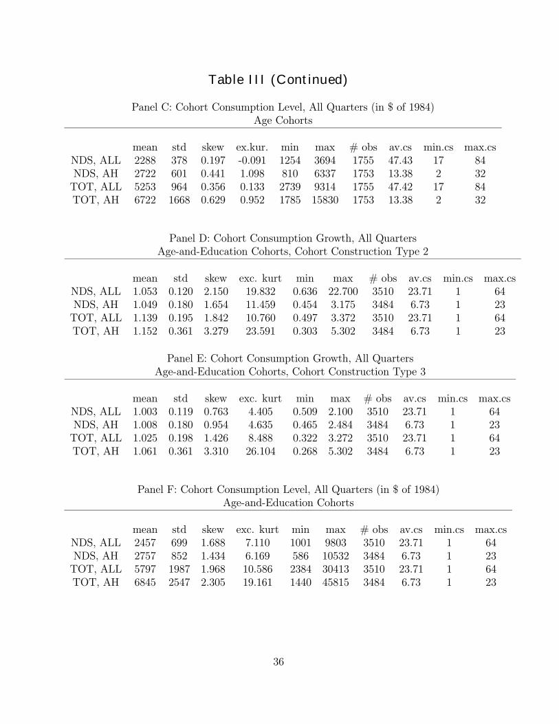
Table III (Continued)

Panel C: Cohort Consumption Level, All Quarters (in $ of 1984)Age Cohorts

mean std skew ex.kur. min max # obs av.cs min.cs max.csNDS, ALL 2288 378 0.197 -0.091 1254 3694 1755 47.43 17 84NDS, AH 2722 601 0.441 1.098 810 6337 1753 13.38 2 32TOT, ALL 5253 964 0.356 0.133 2739 9314 1755 47.42 17 84TOT, AH 6722 1668 0.629 0.952 1785 15830 1753 13.38 2 32

Panel D: Cohort Consumption Growth, All QuartersAge-and-Education Cohorts, Cohort Construction Type 2

mean std skew exc. kurt min max # obs av.cs min.cs max.csNDS, ALL 1.053 0.120 2.150 19.832 0.636 22.700 3510 23.71 1 64NDS, AH 1.049 0.180 1.654 11.459 0.454 3.175 3484 6.73 1 23TOT, ALL 1.139 0.195 1.842 10.760 0.497 3.372 3510 23.71 1 64TOT, AH 1.152 0.361 3.279 23.591 0.303 5.302 3484 6.73 1 23

Panel E: Cohort Consumption Growth, All QuartersAge-and-Education Cohorts, Cohort Construction Type 3

mean std skew exc. kurt min max # obs av.cs min.cs max.csNDS, ALL 1.003 0.119 0.763 4.405 0.509 2.100 3510 23.71 1 64NDS, AH 1.008 0.180 0.954 4.635 0.465 2.484 3484 6.73 1 23TOT, ALL 1.025 0.198 1.426 8.488 0.322 3.272 3510 23.71 1 64TOT, AH 1.061 0.361 3.310 26.104 0.268 5.302 3484 6.73 1 23

Panel F: Cohort Consumption Level, All Quarters (in $ of 1984)Age-and-Education Cohorts

mean std skew exc. kurt min max # obs av.cs min.cs max.csNDS, ALL 2457 699 1.688 7.110 1001 9803 3510 23.71 1 64NDS, AH 2757 852 1.434 6.169 586 10532 3484 6.73 1 23TOT, ALL 5797 1987 1.968 10.586 2384 30413 3510 23.71 1 64TOT, AH 6845 2547 2.305 19.161 1440 45815 3484 6.73 1 23

36

Table IV

Summary Statistics for Consumption-Based Pricing Factors

This table presents descriptive statistics for the three sets of consumption-based pricingfactors. It presents the mean, maximum, minimum and standard deviation of each factorin the sample, which consists of 45 quarterly observations. The Þrst set of factors is basedon consumption data for individual households

mcg1,t = (1/N)NX

i=1

(cgi,t) vcg1,t = (1/N)NX

i=1

(cgi,t −mcg1,t)2

where cgi,t = (ci,t/ci,t−1), ci,t is the consumption of individual i at time t and N is the numberof households in the cross-section. The second and third set of pricing factors are based oncohort data. The second set of factors is obtained by averaging over the consumption growth

of the individuals in that cohort. For cohort j, cohcg2,j,t = (1/Nj,t)PNj,t

i=1 (cgi,t), where Nj,t

is the number of observations on this cohort at time t. Given H cohorts the factors are

mcg2,t = (1/H)HX

j=1

(cohcg2,j,t) vcg2,t = (1/H)HX

j=1

(cohcg2,j,t −mcg2,t)2.

For the second set of factors, consider the average consumption of a representative cohort k

at time t, that is, cohck,t = (1/Nk,t)PNk,t

i=1 (ci,t). DeÞne cohcg3,k,t = (cohck,t/cohck,t−1). Thefactors then are

mcg3,t = (1/H)HX

k=1

(cohcg3,k,t) vcg3,t = (1/H)HX

k=1

(cohcg3,k,t −mcg3,t)2.

37

Table IV (Continued)

Panel A: Nondurable and Services Consumption, All Households

Age Cohorts

mcg1 vcg1 mcg2 vcg2 mcg3 vcg3

mean 1.0491 0.1598 1.0492 0.0040 0.9989 0.0043min 0.9433 0.0879 0.9438 0.0011 0.8884 0.0019max 1.1204 0.4239 1.1249 0.0143 1.0580 0.0184std.dev. 0.0475 0.0774 0.0476 0.0028 0.0500 0.0025

Age-and-Education Cohorts

mcg1 vcg1 mcg2 vcg2 mcg3 vcg3

mean 1.0491 0.1598 1.0523 0.0124 1.0025 0.0122min 0.9433 0.0879 0.9371 0.0052 0.8933 0.0049max 1.1204 0.04239 1.1213 0.0474 1.0718 0.0274std.dev. 0.0475 0.0774 0.0498 0.0079 0.0514 0.0045

Panel B: Nondurable and Services Consumption, Asset Holders

Age Cohorts

mcg1 vcg1 mcg2 vcg2 mcg3 vcg3

mean 1.0510 0.1642 1.0502 0.0158 1.0010 0.0147min 0.9237 0.0821 0.9229 0.0061 0.8724 0.0058max 1.1285 0.7067 1.1354 0.0878 1.0858 0.0676std.dev. 0.0588 0.1184 0.0590 0.0163 0.0579 0.0092

Age-and-Education Cohorts

mcg1 vcg1 mcg2 vcg2 mcg3 vcg3

mean 1.0510 0.1642 1.0497 0.0330 1.0078 0.0321min 0.9237 0.0821 0.9169 0.0157 0.8742 0.0133max 1.1285 0.7067 1.1360 0.1931 1.0972 0.1607std.dev. 0.0588 0.1184 0.0600 0.0268 0.0598 0.0214

38

Table IV (Continued)

Panel C: Total Consumption, All Households

Age Cohorts

mcg1 vcg1 mcg2 vcg2 mcg3 vcg3

mean 1.1355 0.5047 1.1385 0.0132 1.0143 0.0148min 1.0063 0.2475 1.0034 0.0054 0.8923 0.0059max 1.2173 0.8349 1.2166 0.0312 1.0911 0.0265std.dev. 0.0608 0.1217 0.0624 0.0055 0.0582 0.0051

Age-and-Education Cohorts

mcg1 vcg1 mcg2 vcg2 mcg3 vcg3

mean 1.1355 0.5047 1.1385 0.0352 1.0240 0.0368min 1.0063 0.2475 0.9974 0.0141 0.8938 0.0160max 1.2173 0.8349 1.2223 0.0958 1.0990 0.0910std.dev. 0.0608 0.1217 0.0638 0.0154 0.0595 0.0148

Panel D: Total Consumption, Asset Holders

Age Cohorts

mcg1 vcg1 mcg2 vcg2 mcg3 vcg3

mean 1.1436 0.4925 1.1489 0.0521 1.0361 0.0499min 0.9658 0.2385 0.9796 0.0217 0.8563 0.0193max 1.2747 1.1243 1.2787 0.2047 1.1561 0.2162std.dev. 0.0801 0.1569 0.0804 0.0341 0.0723 0.0311

Age-and-Education Cohorts

mcg1 vcg1 mcg2 vcg2 mcg3 vcg3

mean 1.1436 0.4925 1.1504 0.1268 1.0599 0.1280min 0.9658 0.2385 0.9858 0.0478 0.8812 0.0450max 1.2747 1.1243 1.2773 0.3337 1.1842 0.2968std.dev. 0.0801 0.1569 0.0817 0.0660 0.0755 0.0661

39

Table V

Testing for the Significance of Consumption-Based Factors

The following forms of the pricing kernel Mt are tested

Mt(β) = β0 + β1RM,t

Mt(β) = β0 + β1mcgt + β2vcgt

Mt(β) = β0 + β1mcgt + β2vcgt + β3RM,t

where RM,t is the return on the market portfolio, and mcgt and vcgt are the cross-sectionalmean and variance of consumption growth. Our test assets consist of the twenty-Þve Fama-French size and book-to-market portfolios, the long term government bond, the corporatebond, and the T-bill. (See Section 3 for a description of the asset return data.) A standardGMM procedure is implemented for testing the moment conditions E[Mt(β)Rit] = 1, whereRit is the return on the i-th test asset. In the initial round, the HJ-distance measure isminimized. Then the iterated GMM estimates are obtained, i.e., at each round, the weightingmatrix is updated using the estimates from the previous round, and the procedure is repeateduntil estimates converge. Reported in the table are the iterated estimates and the J teststatistics that are based on the iterated estimates. In parentheses under the estimates aret-statistics and in parentheses under the J statistics are the p-values. Reported in panels Athrough D are tests using four different consumption data sets: (i) nondurable and servicesconsumption for all households, (ii) nondurable and services consumption for asset holders,(iii) total consumption for all households, and (iv) total consumption for asset holders.The consumption factors are the three pairs based on consumption growth (mcgj and vcgj,j = 1, 2, 3), deÞned in Table IV (or see Section 3).

40

Table V (Continued)

Panel A: Nondurable and Services Consumption, All Households

row constant mcg1 vcg1 mcg2 vcg2 mcg3 vcg3 RM J-Test

Age Cohorts

1 -2.38 5.94 -18.81 34.00(-0.46) ( 1.20) (-3.85) (0.108)

2 9.50 -7.48 -150.81 38.90( 1.81) (-1.51) (-2.65) (0.038)

3 7.98 -6.75 -64.74 40.01( 1.65) (-1.35) (-0.49) (0.029)

4 26.32 -16.54 -7.74 -6.13 36.40( 3.04) (-2.27) (-2.81) (-1.82) (0.050)

5 59.54 -41.55 -433.30 -12.29 38.98( 7.09) (-5.62) (-4.86) (-3.72) (0.027)

6 15.44 -4.98 -830.64 -6.46 41.78( 2.87) (-0.98) (-5.26) (-3.27) (0.014)

Age-and-Education Cohorts

7 -2.38 5.94 -18.81 34.00(-0.46) ( 1.20) (-3.85) (0.108)

8 12.70 -10.34 -44.74 38.07( 2.13) (-1.85) (-1.87) (0.046)

9 5.89 -3.92 -71.82 39.50( 1.20) (-0.78) (-1.74) (0.033)

10 26.32 -16.54 -7.74 -6.13 36.40( 3.04) (-2.27) (-2.81) (-1.82) (0.050)

11 39.74 -21.80 -49.71 -14.11 36.64( 6.02) (-4.28) (-1.61) (-3.65) (0.048)

12 8.41 4.42 -177.52 -9.16 36.96( 1.49) ( 1.07) (-2.69) (-3.32) (0.044)

13 6.06 -4.94 39.54( 3.17) (-2.72) (0.043)

41

Table V (Continued)

Panel B: Nondurable and Services Consumption, All Assetholders

row constant mcg1 vcg1 mcg2 vcg2 mcg3 vcg3 RM J-Test

Age Cohorts

1 48.97 -38.86 -41.58 30.55( 4.70) (-3.99) (-4.42) (0.204)

2 7.09 -4.81 -72.53 38.07( 1.36) (-0.95) (-2.27) (0.046)

3 21.02 -23.34 194.30 42.73( 6.40) (-7.04) ( 7.72) (0.015)

4 44.53 -32.12 -37.53 -3.37 31.81( 4.50) (-3.56) (-4.02) (-0.81) (0.132)

5 8.44 -5.35 -66.09 -0.85 38.36( 1.38) (-1.06) (-2.10) (-0.30) (0.032)

6 26.88 -14.20 -4.46 -10.95 40.02( 5.01) (-3.01) (-0.12) (-3.93) (0.021)

Age-and-Education Cohorts

7 48.97 -38.86 -41.58 30.55( 4.70) (-3.99) (-4.42) (0.204)

8 -2.15 4.72 -52.89 37.73(-0.52) ( 1.11) (-2.92) (0.049)

9 43.52 -49.11 267.82 31.33( 5.99) (-6.70) ( 5.04) (0.178)

10 44.53 -32.12 -37.53 -3.37 31.81( 4.50) (-3.56) (-4.02) (-0.81) (0.132)

11 12.91 -3.54 -17.90 -7.32 39.36( 2.00) (-0.81) (-0.96) (-2.44) (0.025)

12 43.24 -49.54 264.98 0.75 31.50( 5.88) (-6.65) ( 4.92) ( 0.31) (0.140)

13 6.06 -4.94 39.54( 3.17) (-2.72) (0.043)

42

Table V (Continued)

Panel C: Total Consumption, All Households

row constant mcg1 vcg1 mcg2 vcg2 mcg3 vcg3 RM J-Test

Age Cohorts

1 12.31 -10.22 0.30 41.87( 2.57) (-2.22) ( 0.21) (0.019)

2 17.02 -16.14 164.36 41.41( 5.19) (-5.57) ( 5.55) (0.021)

3 16.21 -20.67 380.76 38.79( 7.60) (-8.43) ( 8.09) (0.039)

4 34.81 -11.00 -1.07 -19.84 37.95( 4.99) (-2.63) (-0.44) (-5.80) (0.035)

5 20.81 -12.12 159.32 -8.01 40.26( 5.04) (-5.52) ( 4.54) (-3.54) (0.020)

6 30.04 -12.76 55.09 -16.15 37.95( 5.23) (-3.67) ( 1.20) (-4.92) (0.035)

Age-and-Education Cohorts

7 12.31 -10.22 0.30 41.87( 2.57) (-2.22) ( 0.21) (0.019)

8 9.93 -7.75 -5.85 41.11( 2.70) (-2.43) (-0.60) (0.022)

9 5.16 -6.20 62.11 39.84( 1.93) (-2.24) ( 3.20) (0.030)

10 34.81 -11.00 -1.07 -19.84 37.95( 4.99) (-2.63) (-0.44) (-5.80) (0.035)

11 71.59 -24.42 -68.08 -38.63 33.14( 6.93) (-4.35) (-2.80) (-7.16) (0.101)

12 34.54 -18.27 141.04 -18.56 33.29( 4.38) (-3.49) ( 4.19) (-4.47) (0.098)

13 6.06 -4.94 39.54( 3.17) (-2.72) (0.043)

43

Table V (Continued)

Panel D: Total Consumption, Asset Holders

row constant mcg1 vcg1 mcg2 vcg2 mcg3 vcg3 RM J-Test

Age Cohorts

1 32.19 -26.13 -0.41 36.67( 4.02) (-3.69) (-0.30) (0.062)

2 36.65 -33.90 70.53 33.76( 5.39) (-5.81) ( 4.52) (0.113)

3 9.17 -9.33 30.41 40.61( 3.17) (-3.40) ( 3.45) (0.025)

4 65.63 -23.94 2.47 -36.77 35.85( 8.20) (-5.96) ( 0.95) (-7.58) (0.057)

5 51.99 -31.01 41.48 -16.59 35.52( 8.11) (-6.25) ( 3.33) (-3.43) (0.061)

6 33.16 -30.26 90.83 -5.23 38.08( 5.14) (-5.97) ( 4.79) (-1.64) (0.034)

Age-and-Education Cohorts

7 32.19 -26.13 -0.41 36.67( 4.02) (-3.69) (-0.30) (0.062)

8 31.68 -28.85 24.20 35.17( 5.06) (-5.27) ( 5.24) (0.085)

9 31.18 -31.45 27.54 35.58( 5.83) (-6.26) ( 6.40) (0.078)

10 65.63 -23.94 2.47 -36.77 35.85( 8.20) (-5.96) ( 0.95) (-7.58) (0.057)

11 58.91 -42.10 21.67 -10.95 26.93( 6.42) (-5.45) ( 3.93) (-2.53) (0.308)

12 38.76 -30.57 33.71 -8.45 36.23( 5.38) (-5.75) ( 4.79) (-2.72) (0.052)

13 6.06 -4.94 39.54( 3.17) (-2.72) 0.043)

44

Table VI

Two Stage GMM and HJ-Distance

The following forms of the pricing kernel Mt are estimated

Mt(β) = β0 + β1RM,t

Mt(β) = β0 + β1mcgt + β2vcgt

Mt(β) = β0 + β1mcgt + β2vcgt + β3RM,t

where RM,t is the return on the market portfolio, and mcgt and vcgt are the cross-sectionalmean and variance of consumption growth. Our test assets consist of the twenty-Þve Fama-French size and book-to-market portfolios, the long term government bond, the corporatebond, and the T-bill. (See Section 3 for a description of the asset return data.) A standardGMM procedure is implemented for testing the moment conditions E[Mt(β)Rit] = 1, whereRit is the return on the i-th test asset. Reported in panel A are the Þrst stage GMMestimates which are the parameter values that minimize the HJ-distance measure. That is,the weighting matrix WHJ =

1T

PTt=1RtR

0t, where Rt is the vector of returns on the test

portfolios. Then the Þrst stage GMM estimates are obtained using this weighting matrix.See Section 4 for more details. In parentheses under the estimates are t-statistics. In panelB are the second stage GMM estimates and the J test statistics. In parentheses under theestimates are t-statistics and in parentheses under the J statistics are the p-values. Thistable is based on the data for the total consumption for asset holders. The consumptionfactors are the three pairs based on consumption growth (mcgj and vcgj, j = 1, 2, 3) derivedfrom the data set of total consumption for asset holders, all deÞned in Table IV.

45

Table VI (Continued)

Panel A: First Stage GMM Estimates and HJ-Distances

row constant mcg1 vcg1 mcg2 vcg2 mcg3 vcg3 RM HJ-d

Age Cohorts

1 16.03 -14.56 3.34 2.33( 2.85) (-2.77) ( 1.37)

2 17.96 -16.82 49.05 2.16( 3.21) (-3.35) ( 2.41)

3 17.00 -18.72 73.86 2.19( 2.41) (-2.39) ( 2.08)

4 26.07 -16.08 2.65 -7.74 2.26( 3.57) (-3.22) ( 0.84) (-1.74)

5 28.04 -18.91 48.36 -7.44 2.10( 3.28) (-3.98) ( 2.34) (-1.28)

6 28.67 -21.98 76.33 -8.19 2.11( 3.06) (-2.97) ( 2.16) (-1.47)

Age-and-Education Cohorts

7 16.03 -14.56 3.34 2.33( 2.85) (-2.77) ( 1.37)

8 14.76 -13.37 13.09 2.29( 2.77) (-2.78) ( 2.31)

9 12.70 -12.97 16.35 2.26( 2.67) (-2.76) ( 2.52)

10 26.07 -16.08 2.65 -7.74 2.26( 3.57) (-3.22) ( 0.84) (-1.74)

11 27.01 -16.28 13.97 -8.77 2.21( 3.52) (-3.19) ( 2.37) (-2.11)

12 23.82 -15.77 16.64 -7.98 2.19( 3.56) (-3.36) ( 2.59) (-2.05)

13 6.77 -5.62 2.41( 2.00) (-1.73)

46

Table VI (Continued)

Panel B: Second Stage GMM Estimates and J Tests

row constant mcg1 vcg1 mcg2 vcg2 mcg3 vcg3 RM J-Test

Age Cohorts

1 14.86 -13.04 2.09 42.24( 3.76) (-3.61) ( 1.68) (0.017)

2 19.89 -18.58 51.23 41.30( 4.74) (-5.09) ( 5.96) (0.021)

3 15.54 -16.79 61.03 40.41( 4.02) (-4.38) ( 4.57) (0.026)

4 26.12 -14.89 1.66 -8.64 41.39( 6.50) (-4.22) ( 1.29) (-3.54) (0.015)

5 31.12 -20.98 49.04 -8.12 40.64( 6.84) (-6.20) ( 4.34) (-2.76) (0.018)

6 27.44 -21.07 68.33 -7.60 41.01( 4.73) (-4.60) ( 4.35) (-3.16) (0.017)

Age-and-Education Cohorts

7 14.86 -13.04 2.09 42.24( 3.76) (-3.61) ( 1.68) (0.017)

8 16.80 -15.16 13.61 42.30( 5.06) (-5.22) ( 5.82) (0.017)

9 13.72 -13.95 16.74 42.45( 5.09) (-5.46) ( 5.25) (0.016)

10 26.12 -14.89 1.66 -8.64 41.39( 6.50) (-4.22) ( 1.29) (-3.54) (0.015)

11 31.41 -19.36 13.37 -9.42 42.04( 6.61) (-6.29) ( 4.06) (-3.19) (0.013)

12 24.74 -16.50 17.43 -8.17 42.27( 6.42) (-6.48) ( 4.70) (-3.37) (0.012)

13 6.68 -5.53 39.56( 3.62) (-3.16) (0.043)

47

Table VII

Testing for the Significance of Consumption Growth

The following forms of the pricing kernel Mt are tested

Mt(β) = β0 + β1mcgt

Mt(β) = β0 + β1mcgt + β2RM,t + β3SMBt + β4HMLt

where SMB and HML are the size and book-to-market factors of Fama and French, and mcgt

is the cross-sectional mean of consumption growth. Our test assets consist of the twenty-Þve Fama-French size and book-to-market portfolios, the long term government bond, thecorporate bond, and the T-bill. (See Section 3 for a description of the asset return data.) Astandard GMM procedure is implemented for testing the moment conditions E[Mt(β)Rit] =1, where Rit is the return on the i-th test asset. In the initial round, the HJ-distance measureis minimized. Then the iterated GMM estimates are obtained, i.e., at each round, theweighting matrix is updated using the estimates from the previous round, and the procedureis repeated until estimates converge. Reported in the table are the iterated estimates andthe J test statistics that are based on the iterated estimates. In parentheses under theestimates are t-statistics and in parentheses under the J statistics are the p-values. The HJdistances are also included. The consumption factors (mcgj, j = 2, 3) are constructed withthe age cohorts and age-education cohorts, respectively, derived from the data set of totalconsumption for asset holders. All the consumption factors are deÞned in Table IV.

48

Table VII (Continued)

row const. mcg1 mcg2 mcg3 RM SMB HML J-Test HJ-d

Age Cohorts

1 34.31 -28.14 36.68 2.36( 4.63) (-4.46) (0.080)

2 15.83 -12.56 40.21 2.39( 2.85) (-2.65) (0.037)

3 6.80 -5.62 40.37 2.42( 1.97) (-1.71) (0.036)

4 76.22 -30.41 -38.32 -14.10 -23.70 31.17 2.18( 7.19) (-6.06) (-4.43) (-2.18) (-2.90) (0.119)

5 67.12 -19.46 -41.34 -5.02 -33.41 28.60 2.22( 6.15) (-4.29) (-5.71) (-1.05) (-5.55) (0.194)

6 58.82 -15.48 -39.34 0.28 -31.60 28.59 2.29( 6.23) (-3.49) (-6.33) ( 0.07) (-6.73) (0.194)

Age-and-Education Cohorts

7 34.31 -28.14 36.68 2.36( 4.63) (-4.46) (0.080)

8 10.00 -7.75 39.85 2.38( 2.86) (-2.60) (0.040)

9 7.48 -6.13 39.75 2.41( 2.42) (-2.14) (0.041)

10 76.22 -30.41 -38.32 -14.10 -23.70 31.17 2.18( 7.19) (-6.06) (-4.43) (-2.18) (-2.90) (0.119)

11 68.40 -34.34 -26.67 -24.09 -22.12 28.99 2.21( 6.49) (-5.44) (-3.33) (-3.10) (-3.40) (0.181)

12 103.08 -32.79 -63.44 -4.28 -47.90 26.05 2.27( 8.93) (-5.98) (-7.12) (-0.67) (-7.75) (0.299)

49

Table VIII

Testing for Significance of Consumption-Based Factorsin the Presence of the Size and Book-to-Market Factors

The following forms of the pricing kernel Mt are tested

Mt(β) = β0 + β1SMBt + β2HMLt

Mt(β) = β0 + β1RM,t + β2SMBt + β3HMLt

Mt(β) = β0 + β1mcgt + β2vcgt + β3SMBt + β4HMLt

Mt(β) = β0 + β1mcgt + β2vcgt + β3RM,t + β4SMBt + β5HMLt

where SMB and HML are the size and book-to-market factors of Fama and French, mcgt

and vcgt are cross-sectional mean and variance of consumption growth. Our test assetsconsist of the twenty-Þve Fama-French size and book-to-market portfolios, the long termgovernment bond, the corporate bond, and the T-bill. (See Section 3 for a description ofthe asset return data.) A standard GMM procedure is implemented for testing the momentconditions E[Mt(β)Rit] = 1, whereRit is the return on the i-th test asset. In the initial round,the HJ-distance measure is minimized. Then the iterated GMM estimates are obtained, i.e.,at each round, the weighting matrix is updated using the estimates from the previous round,and the procedure is repeated until estimates converge. Reported in the table are the iteratedestimates and the J test statistics that are based on the iterated estimates. In parenthesesunder the estimates are t-statistics and in parentheses under the J statistics are the p-values.The HJ distances are also included. The factors are constructed with the age cohorts andage-education cohorts, respectively, derived from the data set of total consumption for assetholders. The consumption factors are the two pairs based on consumption growth (mcgj andvcgj, j = 2, 3). These factors are deÞned in Table IV.

50

Table VIII (Continued)

const. mcg2 vcg2 mcg3 vcg3 RM SMB HML J-Test HJ-d

1.03 2.50 -3.73 38.27 2.43(20.09) ( 0.79) (-1.49) (0.043)

20.28 -17.92 49.98 -20.99 31.45 2.35( 7.97) (-7.42) ( 9.04) (-4.45) (0.141)

Age Cohorts

50.40 -45.96 67.85 -34.30 -10.52 20.15 2.15( 7.75) (-8.40) ( 3.30) (-5.34) (-1.76) (0.633)23.15 -26.59 122.60 33.59 54.36 30.14 2.18( 4.78) (-5.03) ( 4.73) ( 4.06) ( 7.92) (0.145)

68.96 -29.97 28.77 -33.15 8.12 -34.32 27.65 2.02( 6.45) (-4.38) ( 1.79) (-5.29) ( 0.96) (-4.96) (0.188)80.73 -36.45 78.42 -43.47 12.36 -33.90 29.13 2.04( 7.65) (-4.95) ( 2.54) (-6.52) ( 2.03) (-6.07) (0.141)

Age-and-Education Cohorts

42.21 -38.13 23.26 -27.08 -4.10 27.69 2.26( 5.76) (-6.14) ( 4.34) (-4.10) (-0.87) (0.228)29.99 -29.83 19.87 -15.72 3.27 33.91 2.24( 5.26) (-5.64) ( 4.31) (-3.07) ( 1.00) (0.067)

75.72 -37.70 14.02 -31.26 -5.69 -32.65 24.43 2.05( 7.14) (-5.59) ( 2.71) (-4.51) (-0.80) (-4.03) (0.325)72.31 -41.88 24.32 -28.53 -15.38 -20.54 28.56 2.07( 6.70) (-5.89) ( 3.49) (-3.92) (-2.33) (-2.89) (0.158)

51

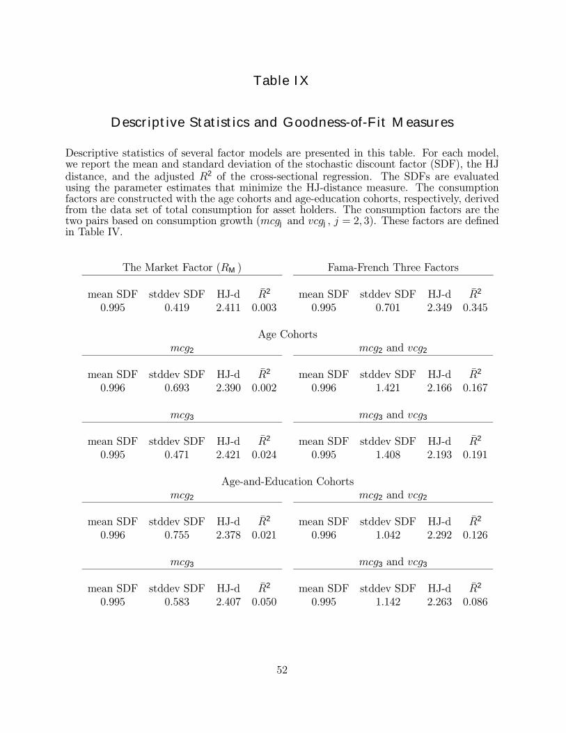
Table IX

Descriptive Statistics and Goodness-of-Fit Measures

Descriptive statistics of several factor models are presented in this table. For each model,we report the mean and standard deviation of the stochastic discount factor (SDF), the HJdistance, and the adjusted R2 of the cross-sectional regression. The SDFs are evaluatedusing the parameter estimates that minimize the HJ-distance measure. The consumptionfactors are constructed with the age cohorts and age-education cohorts, respectively, derivedfrom the data set of total consumption for asset holders. The consumption factors are thetwo pairs based on consumption growth (mcgj and vcgj, j = 2, 3). These factors are deÞnedin Table IV.

The Market Factor (RM) Fama-French Three Factors

mean SDF stddev SDF HJ-d R2 mean SDF stddev SDF HJ-d R2

0.995 0.419 2.411 0.003 0.995 0.701 2.349 0.345

Age Cohortsmcg2 mcg2 and vcg2

mean SDF stddev SDF HJ-d R2 mean SDF stddev SDF HJ-d R2

0.996 0.693 2.390 0.002 0.996 1.421 2.166 0.167

mcg3 mcg3 and vcg3

mean SDF stddev SDF HJ-d R2 mean SDF stddev SDF HJ-d R2

0.995 0.471 2.421 0.024 0.995 1.408 2.193 0.191

Age-and-Education Cohortsmcg2 mcg2 and vcg2

mean SDF stddev SDF HJ-d R2 mean SDF stddev SDF HJ-d R2

0.996 0.755 2.378 0.021 0.996 1.042 2.292 0.126

mcg3 mcg3 and vcg3

mean SDF stddev SDF HJ-d R2 mean SDF stddev SDF HJ-d R2

0.995 0.583 2.407 0.050 0.995 1.142 2.263 0.086

52

Liste des publications au CIRANO*

Série Scientifique / Scientific Series (ISSN 1198-8177)

2002s-11 Idiosyncratic Consumption Risk and the Cross-Section of Asset Returns / Kris Jacobset Kevin Q. Wang

2002s-10 The Demand for the Arts / Louis Lévy-Garboua et Claude Montmarquette2002s-09 Relative Wealth, Status Seeking, and Catching Up / Ngo Van Long, Koji Shimomura2002s-08 The Rate of Risk Aversion May Be Lower Than You Think / Kris Jacobs2002s-07 A Structural Analysis of the Correlated Random Coefficient Wage Regression Model

/ Christian Belzil et Jörgen Hansen2002s-06 Information Asymmetry, Insurance, and the Decision to Hospitalize / Åke Blomqvist

et Pierre Thomas Léger2002s-05 Coping with Stressful Decisions: Individual Differences, Appraisals and Choice /

Ann-Renée Blais2002s-04 A New Proof Of The Maximum Principle / Ngo Van Long et Koji Shimomura2002s-03 Macro Surprises And Short-Term Behaviour In Bond Futures / Eugene Durenard et

David Veredas2002s-02 Financial Asset Returns, Market Timing, and Volatility Dynamics / Peter F.

Christoffersen et Francis X. Diebold2002s-01 An Empirical Analysis of Water Supply Contracts / Serge Garcia et Alban

Thomas2001s-71 A Theoretical Comparison Between Integrated and Realized Volatilities Modeling

/ Nour Meddahi2001s-70 An Eigenfunction Approach for Volatility Modeling / Nour Meddahi2001s-69 Dynamic Prevention in Short Term Insurance Contracts / M. Martin Boyer et

Karine Gobert2001s-68 Serial Cost Sharing in Multidimensional Contexts / Cyril Téjédo et Michel

Truchon2001s-67 Learning from Strike / Fabienne Tournadre et Marie-Claire Villeval2001s-66 Incentives in Common Agency / Bernard Sinclair-Desgagné2001s-65 Detecting Mutiple Breaks in Financial Market Volatility Dynamics / Elena

Andreou et Eric Ghysels2001s-64 Real Options, Preemption, and the Dynamics of Industry Investments / Marcel Boyer,

Pierre Lasserre, Thomas Mariotti et Michel Moreaux2001s-63 Dropout, School Performance and Working while in School: An Econometric Model

with Heterogeneous Groups / Marcel Dagenais, Claude Montmarquette et NathalieViennot-Briot

2001s-62 Derivatives Do Affect Mutual Funds Returns : How and When? / Charles Cao,Eric Ghysels et Frank Hatheway

* Consultez la liste complète des publications du CIRANO et les publications elles-mêmes sur notre site Internet :

http://www.cirano.qc.ca/publication/documents.html

2001s-61 Conditional Quantiles of Volatility in Equity Index and Foreign Exchange Data /John W. Galbraith, Serguei Zernov and Victoria Zinde-Walsh

2001s-60 The Public-Private Sector Risk-Sharing in the French Insurance "Cat. Nat.System" / Nathalie de Marcellis-Warin et Erwann Michel-Kerjan

2001s-59 Compensation and Auditing with Correlated Information / M. Martin Boyer etPatrick González

2001s-58 Resistance is Futile: An Essay in Crime and Commitment / M. Martin Boyer2001s-57 The Unreliability of Output Gap Estimates in Real Time / Athanasios Orphanides

et Simon van Norden2001s-56 Exact Nonparametric Two-Sample Homogeneity Tests for Possibly Discrete

Distributions / Jean-Marie Dufour et Abdeljelil Farhat2001s-55 Les coûts de la réglementation : une revue de la littérature / Robert Gagné, Paul

Lanoie, Pierre-Carl Micheud et Michel Patry2001s-54 Testing for structural Change in the Presence of Auxiliary Models / Eric Ghysels

et Alain Guay2001s-53 Environmental Regulation and Productivity: New Findings on the Porter

Hypothesis / Paul Lanoie, Michel Patry et Richard Lajeunesse2001s-52 The Aftermarket Performance of Initial Public Offerings in Canada / Maher Kooli

et Jean-Marc Suret2001s-51 Capital Structure and Risk Management / Karine Gobert2001s-50 The Underpricing of Initial Public Offerings: Futher Canadian Evidence / Maher

Kooli et Jean-Marc Suret2001s-49 How Innovative Are Canadian Firms Compared to Some European Firms? A

Comparative Look at Innovation Surveys / Pierre Mohnen et Pierre Therrien2001s-48 A Tale of Two Ports / Ngo Van Long et Kar-yiu Wong2001s-47 Wage Policy of Firms: An Empirical Investigation / Stéphanie Lluis2001s-46 Forecasting Some Low-Predictability Time Series Using Diffusion Indices / Marc

Brisson, Bryan Campbell et John W. Galbraith2001s-45 The Importance of the Loss Function in Option Pricing / Peter Christoffersen et

Kris Jacobs2001s-44 Let's Get "Real" about Using Economic Data / Peter Christoffersen, Eric Ghysels

et Norman R. Swanson2001s-43 Fragmentation, Outsourcing and the Service Sector / Ngo Van Long, Ray

Riezman et Antoine Soubeyran2001s-42 Nonlinear Features of Realized FX Volatility / John M. Maheu et Thomas H.

McCurdy2001s-41 Job Satisfaction and Quits: Theory and Evidence from the German

Socioeconomic Panel / Louis Lévy-Garboua, Claude Montmarquette et VéroniqueSimonnet

2001s-40 Logique et tests d'hypothèse : réflexions sur les problèmes mal posés enéconométrie / Jean-Marie Dufour