Expected Taxes and Household Consumption Behavior by ...

Expected Taxes and Household Consumption Behavior

by

Lorenz Kueng

A dissertation submitted in partial satisfaction of the

requirements for the degree of

Doctor of Philosophy

in

Economics

in the

Graduate Division

of the

University of California, Berkeley

Committee in charge:

Professor Alan Auerbach, Co-chair

Professor Yuriy Gorodnichenko, Co-chair

Professor Emmanuel Saez

Professor Dwight Jaffee

Spring 2012

Abstract

Expected Taxes and Household Consumption Behavior

by

Lorenz Kueng

Doctor of Philosophy in Economics

University of California, Berkeley

Alan Auerbach, Co-chair

Yuriy Gorodnichenko, Co-chair

In this dissertation I ask two basic questions: First, how predictable are personalincome tax changes in the U.S. and second, does household consumption respond tonews about future tax changes, or does it mostly respond at the time when the taxrates actually change? These are interesting questions because they have broad im-plications for macroeconomics and public economics.The rational-expectations life-cycle theory of consumption is the workhorse in modern macroeconomics. Whilethere are various specifications of this theory, two predictions are common acrossthem. First, consumption should not respond to predictable income changes andsecond, consumption should respond to news about future after-tax lifetime income.There is a large literature that tests the first implication of the rational-expectationslife-cycle theory and generally rejects the model by finding significant consumptionresponses to predictable income changes – that is, it finds that consumption is infact excessively sensitive to predictable income changes. Very few studies focus onthe theory’s second main prediction, that household consumption responds to newsabout after-tax income changes, even if current after-tax income has not changedyet. To the best of my knowledge this dissertation is indeed the first study to usemicro-level data to estimate the consumption response to news.

I use fiscal policy to study these two questions because it offers two main ad-vantages over other empirical frameworks commonly used by macroeconomists totest the consumption theory and to analyze the effect of news on macroeconomicaggregates. First, exploiting the fact that there is a lag between the decision tochange taxes and the implementation of the tax changes allows me to separate thebehavioral response to news from the response to the actual policy changes. There-fore, the response to tax news is not confounded by the response to the actual taxchange. Second, actual tax changes are directly observable without measurementissues, which is different from other news shocks that have been recently studied,in particular news about future total factor productivity. Therefore, my measure ofnews about future taxes can be directly compared with the actual evolution of the

1

tax rates.Regarding public economics, this dissertation addresses another question that is

of interest to public policy makers. During the current Great Recession, in whichconventional monetary policy is not effective due to the zero lower bound on nominalinterest rates, policy makers have shifted attention to fiscal interventions. In orderto assess the effectiveness of fiscal policy we have to know the total effect of a taxreform on the economy, i.e. the tax multiplier. Unfortunately, almost all studiesthat provide estimates of tax multipliers focus on the response of the economy toactual tax changes. These estimates might miss a fraction of the total effect of atax reform if tax changes are predictable and if the behavior of economic agents isforward-looking. Ignoring anticipation effects can therefore bias the tax multiplierdownward.

The identification of news about future tax rates is key for answering these ques-tions. In this dissertation I exploit the fact that there exist two classes of fixed-income securities in the U.S. that are very similar except for the tax treatment oftheir income streams. Interest on municipal bonds is tax-exempt, while interest onTreasury bonds is subject to federal income taxes; thus, relative price changes be-tween municipal and Treasury bonds reflect changes in expected future tax rates,holding fixed other risk factors. I go beyond identification of the timing of news todirectly measure the entire path of expected tax rates. The fact that different bondshave different maturities quantifies the degree of tax foresight, since yield spreads ofbonds with different maturities reflect information about future taxes over differenthorizons. Hence, the tax news shocks derived from the bond prices measure not onlywhen households receive information, but also what information they receive.

Identifying the entire path of expected tax rates in turn is important for testingthe basic rational-expectations life-cycle model of consumption, as the theory pre-dicts that consumption responds one-for-one to changes in expected after-tax life-time income. The term structure of municipal yield spreads identifies the expectedpersistence of a tax shock, which is a crucial factor that determines the optimal con-sumption response according to the theory. For instance, if a tax change is expectedto be only transitory, then the theory predicts that consumption does not respondmuch. On the other hand, if a tax reform is expected to have a large persistentcomponent, then consumption should respond much stronger.

Combining these market-based tax expectations with consumption data from theConsumer Expenditure Survey I find that consumption of high-income householdsincreases by close to 1% in response to news of a 1% increase in expected after-tax lifetime income, consistent with the basic rational-expectations life-cycle theory.On the other hand, households who have lower income, less education, or are morecredit constrained respond less to news. However, the same households also respondone-for-one with large news shocks, consistent with rational inattention.

2

To my parents, Susanna and Martin, my wife Sandra, and my daughter Sophia

i

Contents

1 The Taxation of Bonds 11.1 Introduction . . . . . . . . . . . . . . . . . . . . . . . . . . . . . . . . 11.2 Taxation of Taxable Bonds . . . . . . . . . . . . . . . . . . . . . . . . 4

1.2.1 Original-Issue Discount (OID) Bonds . . . . . . . . . . . . . . 41.2.2 Market Discount (MD) Bonds . . . . . . . . . . . . . . . . . . 51.2.3 Premium (MP) Bonds . . . . . . . . . . . . . . . . . . . . . . 6

1.3 Taxation of Tax-Exempt Bonds . . . . . . . . . . . . . . . . . . . . . 71.3.1 Original-Issue Discount (OID) Bonds . . . . . . . . . . . . . . 71.3.2 Market Discount (MD) Bonds . . . . . . . . . . . . . . . . . . 71.3.3 Premium (MP) Bonds . . . . . . . . . . . . . . . . . . . . . . 81.3.4 Callable Bonds . . . . . . . . . . . . . . . . . . . . . . . . . . 8

1.4 Valuation of Bonds using After-Tax Cash Flows . . . . . . . . . . . . 81.4.1 Original-Issue Discount (OID) Bonds . . . . . . . . . . . . . . 91.4.2 Market Discount (MD) Bonds . . . . . . . . . . . . . . . . . . 101.4.3 Premium (MP) Bonds . . . . . . . . . . . . . . . . . . . . . . 11

1.5 Dealing with Accrued Interest . . . . . . . . . . . . . . . . . . . . . . 12

2 The Household Consumption Response to Tax News 132.1 Introduction . . . . . . . . . . . . . . . . . . . . . . . . . . . . . . . . 132.2 Tax Expectations from Municipal Yield Spreads . . . . . . . . . . . . 18

2.2.1 Factors other than Expected Tax Rates . . . . . . . . . . . . . 192.2.2 A Model of Break-Even Tax Rates (BETR) . . . . . . . . . . 212.2.3 The Marginal Tax Rate of the Marginal Investor . . . . . . . . 242.2.4 Two Presidential Elections as Natural Experiments . . . . . . 272.2.5 Deriving Expected Tax Rates from Break-Even Tax Rates . . 30

2.3 Household Consumption Response to Tax News . . . . . . . . . . . . 342.3.1 Two Sources of Identification . . . . . . . . . . . . . . . . . . 412.3.2 Consumption Response of High-Income Households . . . . . . 422.3.3 Consumption Response in the Full Sample . . . . . . . . . . . 432.3.4 Understanding the Different Responses . . . . . . . . . . . . . 43

2.4 Conclusion . . . . . . . . . . . . . . . . . . . . . . . . . . . . . . . . . 45

ii

3 Documentation and Extensions 483.1 Data . . . . . . . . . . . . . . . . . . . . . . . . . . . . . . . . . . . . 48

3.1.1 Bond Data . . . . . . . . . . . . . . . . . . . . . . . . . . . . . 483.1.2 Flow of Funds . . . . . . . . . . . . . . . . . . . . . . . . . . . 493.1.3 Survey of Consumer Finances (SCF) . . . . . . . . . . . . . . 493.1.4 Election Probabilities . . . . . . . . . . . . . . . . . . . . . . . 503.1.5 Consumer Expenditure Survey (CEX) . . . . . . . . . . . . . 50

3.2 Historical Bond Default Rates . . . . . . . . . . . . . . . . . . . . . . 513.3 Pre-Refundend Municipal Bonds and Rare Default Events . . . . . . 523.4 State CDS Spreads . . . . . . . . . . . . . . . . . . . . . . . . . . . . 523.5 The Markets for Treasury and Municipal Bonds . . . . . . . . . . . . 533.6 Robust Inverse . . . . . . . . . . . . . . . . . . . . . . . . . . . . . . 533.7 Linear Approximation of the Expected Tax Liability . . . . . . . . . . 553.8 Tax Base and Robustness across Sub-Periods . . . . . . . . . . . . . . 563.9 Different Time Series Filters . . . . . . . . . . . . . . . . . . . . . . . 57

A Tables 58

B Figures 74

iii

List of Tables

A.1 StateTaxation . . . . . . . . . . . . . . . . . . . . . . . . . . . . . . . 59A.2 presidential elections of 2000 and 1992 . . . . . . . . . . . . . . . . . 61A.5 HistoricalBondDefaultRates . . . . . . . . . . . . . . . . . . . . . . . 62A.3 Consumption response to tax news shocks . . . . . . . . . . . . . . . 63A.4 Consumption response to tax news shocks in the full sample: extensions 64A.6 Presidential election of 2000 . . . . . . . . . . . . . . . . . . . . . . . 65A.7 Presidential election of 1992 . . . . . . . . . . . . . . . . . . . . . . . 67A.8 Consumption response of high-income households in different sub-

periods. . . . . . . . . . . . . . . . . . . . . . . . . . . . . . . . . . . 69A.9 Consumption response of high-income households: different filtering. . 70A.10 Consumption response as a function of the size of the tax news shock. 71A.11 Consumption response as a function of liquid wealth. . . . . . . . . . 72A.12 Consumption response as a function of education. . . . . . . . . . . . 73

iv

List of Figures

B.1 Evolution of the tax basis of a hypothetical 30-year bond purchasedfive years after issue. . . . . . . . . . . . . . . . . . . . . . . . . . . . 75

B.2 Yields of AAA general-obligation (GO) bonds of states with differenttax treatment of in- and out-of-state investors. . . . . . . . . . . . . 76

B.3 2-year and 15-year break-even tax rates (BETR) θt,2 and θt,15 againstthe marginal tax rate of the top 1%. . . . . . . . . . . . . . . . . . . 77

B.4 Average Marginal Tax Rate of the Marginal Investors calculated fromthe Survey of Consumer Finances (SCF). . . . . . . . . . . . . . . . 78

B.5 Path of Break-Even Tax Rates during presidential election of 2000. . 79B.6 Path of Break-Even Tax Rates during presidential election of 1992. . 80B.7 Path of Expected Tax Rates during presidential election of 2000. . . 81B.8 Path of Expected Tax Rates during presidential election of 1992. . . 82B.9 Average break-even tax premium E[Λt] as a function of the maturity;

see equation (2.9). . . . . . . . . . . . . . . . . . . . . . . . . . . . . 83B.10 Anticipation of the Reagan Tax Cuts (ERTA 1981 and TRA 1986)

between January 1977 and January 1982. . . . . . . . . . . . . . . . 84B.11 Change in the average tax rate caused by income tax reforms between

1980 and 2003. . . . . . . . . . . . . . . . . . . . . . . . . . . . . . . 85B.12 Spread between AAA general-obligation and pre-refunded municipal

bonds with 7-year maturity. . . . . . . . . . . . . . . . . . . . . . . . 86B.13 Credit Default Swap (CDS) of 10-year Treasury, municipal, and cor-

porate bonds. . . . . . . . . . . . . . . . . . . . . . . . . . . . . . . 87B.14 Different filtering of the time series of 2-year break-even tax rates. . 88B.15 Municipal Debt Ownership . . . . . . . . . . . . . . . . . . . . . . . 89B.16 Total federal Average Tax Rates 1977-2007 . . . . . . . . . . . . . . 90

v

Acknowledgments

Above all, I would like to thank my parents, Susanna and Martin, and my wifeSandra for always being so patient, understanding, and supportive. I hope thatSophia will forgive me for missing her first birthday while being on the job market.

I am especially grateful to Alan Auerbach and Yuriy Gorodnichenko for theirencouragement and support throughout this project; it is hard to imagine a betterteam of advisors. Alan and Yuriy are true role models, and it will be a challengeand privilege to emulate them as I start my next step as an academic researcher.

I am indebted to Henner Kleinewefers who first sparked my interest in economics,and to Mark Schelker and Andreas Fuster for encouraging me to pursue my graduatestudies abroad. I am grateful to George Akerlof for teaching me new approachesto macroeconomics. I was lucky to have had the opportunity to learn empiricalmacroeconomics from Christy and David Romer, who taught me that creativitytrumps tools, and that careful data work is king.

I had the fortune to learn from many of my outstanding peers, in particular Mu-Jeung Yang, Bryan Hong, and Evgeny Yakovlev. My time spent in Evans Hall wouldhave been much less fun without my office mates, in particular Gisela Rua, Nick Li,Dean Scrimgeour, Josh Hausman, and Yury Yatsynovich.

I also benefited from many conversations with people across different fields whoencouraged me to look at the same questions from different angles. David Card,Pierre-Olivier Gourinchas, Dwight Jaffee, Patrick Kline, Nick Li, Ulrike Malmendier,Dina Pomeranz, Demian Pouzo, Emmanuel Saez, Adam Szeidl, Mu-Jeung Yang; sem-inar participants at the Universities of Basel, Barcelona, Berkeley, Columbia, North-western, Santa Barbara LAEF, Stockholm, Toronto, Toulouse, Virginia, Washington;the Federal Reserve Banks of Boston, Kansas City, New York, and San Francisco;the Bank of Finland, Dartmouth College, ETH Zurich, Penn State University, andthe Study Center Gerzensee all provided valuable feedback on Chapters 2 and 3. Ithank Daniel Feenberg for support with mapping the CEX to TAXSIM, Kevin Moorefor sharing his code for the SCF, and Craig Kreisler for patiently answering all myquestions about the CEX.

vi

Chapter 1

The Taxation of Bonds

This chapter explains what researchers who are interested in bond pricing shouldknow about the taxation of fixed-income securities. It provides necessary backgroundinformation for the analysis in Chapter 2. The taxation of fixed-income securitiesin the U.S. is complex, but important for understanding the pricing of bonds. Thischapter presents the different tax rules since 1970 are formalized them within a basicasset pricing framework.

1.1 Introduction

Before looking at the tax treatment of different types of bonds I need to introducesome notation and I need to define some terms that might not be familiar to mostresearchers. I then derive the implications of federal taxation on the pricing of bonds.

Notation I use the following notation to formalize the tax treatment of fixed-income securities.

Pt : bond price at time t .

P it : adjusted issue price, with P i

ti= Pti being the issue price.

P pt : adjusted purchase price, with P p

tp = Ptp being the purchase price.

Ptm : redemption value, usually normalized such that Ptm = 1.

ti : issue date.

tm : maturity date.

tp : purchase date.

1

1.1. INTRODUCTION

ts : selling date, with ts = t+ s , where s is the planed holding period with 0 < s ≤m .

mo,m : original and remaining maturity of the bond in years,where m and mo are defined as tm = ti +mo = t+m .

At : accrued interest up to t since last payment at t , At = t−t1/aC .

a : number of payments per year, i.e. inverse of payment frequency f = 1/a . Hence,m · a are the total remaining payments.

c : coupon rate applied to the bond’s redemption value to determine the couponpayment C = Ptm

ca

.

dt(k) : after-tax nominal discount function between period t and t+k, which knownat t, dt(k) ≡ dt,k .

τ y, τ g : income and capital gains tax rates of the investor.

Some Jargon Three concepts are important to determine the path of tax liabilitiesfor fixed-income securities.1

• The adjusted issue price P it defines the original issue discount (OID) and its

(continuous) amortization over the asset’s lifetime.

• The adjusted purchase price (or tax basis) P pt defines the market discount

(MD) or premium (MP) and its amortization over time as well as the amountof capital gains if the bond is sold prior to maturity.

• The DeMinimis bound DM(P,m) determines whether the amortization ofthe OID and the MD, which generates hypothetical interest income in additionto the actual coupon payment, has to be taken into account for taxation. TheDeMinimis bound is a function of the bond’s maturity m and price P and isdefined as

DM(P,m) = P ·(

1− m

400

).

These concepts define four types of bonds:

1. OID bonds with Pti < Ptm ,

2. MD bonds with Ptp < P itp , and

1 For a discussion of the tax treatment of investors other than individuals or corporations suchas traders and dealers, see Fabozzi and Nirenberg (1991).

2

1.1. INTRODUCTION

3. (market) premium bonds (MP), and more specific

(a) premium bonds – either original issue or secondary market – with Ptp >Ptm and

(b) acquisition premium bonds with Ptp ∈ (P itp , Ptm) and P i

tp < Ptm .2

For tax purposes, the acquisition and the pure market premium bonds are treatedvery similar so that we only have to analyze three types of bonds separately. The priceof OID, MD, and acquisition MP bonds will appreciate until maturity everything elseequal, while the price of a pure MP bond will depreciate. Note that a par bond forwhich Pti = Ptm is a particular OID bond with OID= 0 and has the same taxtreatment as a general OID bond.

The prices P it and P p

t are adjusted using either a ratable method (RM) – i.e. astraight-line method – or a constant yield method (CYM) depending on the date ofissue and the owner’s tax preferences. The adjusted price according to the CYM is

P xtx,k = P x

tx,k−1 · (1 + ytx/a)− Ptmc/a

= Ptx (1 + ytx/a)k − Ptmc/ak∑i=1

(1 + ytx/a)i−1 ,

where ytx is the constant yield to maturity at purchase date tx and x ∈ {i, p} .3 Theadjusted price according to the ratable method (RM) is

P xtx,k = P x

tx + ∆k

m · a .

∆ is either the OID in which case ∆ = Ptm − Pti > 0 , the market discount in whichcase ∆ = P i

tp −Ptp > 0 , the (market) premium in which case ∆ = Ptp −Ptm > 0 , orthe acquisition premium in which case ∆ = Ptp−Pti > 0 with Ptp < Ptm . Figure B.1graphs these concepts together with the corresponding DeMinimis bounds.

The amortized discount or premium (OID, MD, or MP) that has to be includedin current income is based on the number of days in the tax year that the bond isheld. The tax treatment of the bond – i.e. which tax rate applies, which amortization

2 In practice, an acquisition premium bond is still called a discount bond since it trades belowpar, i.e. Ptp < Ptm .

3 The constant yield to maturity yt is defined as the solution to the equation

PtPtm

=c

a

m·a∑k=1

(1 + yt/a)−k

+ (1 + yt/a)−m·a

where m is the remaining maturity of the bond. If the date t does not coincide with a paymentdate, then accrued interest has to be added as shown below. One can verify that the formula forthe adjusted price P xtx,k satisfies P xtx,0 = Ptx and P xtx,ma = Ptma.

3

1.2. TAXATION OF TAXABLE BONDS

method is chosen, when the amortization is applied, and how capital gains are defined– depends on the issuer of the bond (corporate, Treasury, or municipal), the issuedate, the type of investor (individual or corporation), and the type of the bond listedabove (OID, MD, or MP bond).

1.2 Taxation of Taxable Bonds

Interest income from Treasury bonds is exempt from state and local taxes inall states except Tennessee but is subject to federal income taxes. Bonds issuedby states, which are part of the class of municipal bonds, are exempt from federalincome taxes. Moreover, most states also exempt municipal bonds from state andlocal taxes, either for all investors or at least for instate investors. Table A.1 liststhe tax treatment of fixed-income interest in all fifty states and Washington D.C.

If not stated otherwise, the following tax rules apply to both Treasury and cor-porate bonds.4 However, note that corporate bonds are in general subject to bothfederal taxes and state and local taxes. Moreover, many investors can deduct at leastpart of their state and local income taxes from their federal income taxes. Theseissues have to be taken into account when analyzing the effects of taxes on corporatebond prices.

Different tax treatments apply to taxable bonds depending on the types of bondas well as the bond’s issue date. The following is a summary of these tax rules andtheir evolution since 1970.

1.2.1 Original-Issue Discount (OID) Bonds

The DeMinimis rule applies. If Pti > DM(Ptm ,mo) then the OID is ignored fortax purposes and is taxed as (unexpected) capital gain at sale or maturity. Thefollowing rules depend on the bond’s date of issue.

• Issued between 5/29/69 and 7/2/82

– Corporate bonds: The OID is amortized linearly (RM) and included incurrent ordinary interest income.

– Treasury bonds: The OID is treated as capital gains income at sale ormaturity.

4 For short-term non-coupon bearing obligations (e.g. Treasury bills), callable or putable bonds,and more exotic bonds such as stripped or principal obligations, see Fabozzi (2002) and Kramer(2003).

4


• Issued on or after 7/2/82

– The OID is amortized with CYM using annual compounding (a = 1).

– The OID is included in current ordinary interest income.

• Issued after 12/31/84

– The OID is amortized with CYM using at least semi-annual compoundingor compounding corresponding to the payment frequency (a ≥ 2).

1.2.2 Market Discount (MD) Bonds

The DeMinimis rule applies to the MD. If Ptp > DM(P itp ,m) , then the MD is

ignored for tax purposes and is taxed as (unexpected) capital gain at sale or maturity.The following rules depend on the bond’s date of issue.

• Issued before 7/19/84

– MD is treated as capital gain income at sale or maturity. Hence theadjusted purchase price does not matter for taxation, i.e.

MDts = 0

and the capital gains are

total price change︷︸︸︷(Pts − Ptp) −

accrued OID up to ts︷︸︸︷(P i

ts − P itp)


– The MD is treated as ordinary income at sale or maturity.5

– The adjusted purchase price can be determined with the CYM (or linearlybut this is usually not optimal).

– The amount of accrued market discount that is included in ordinary in-come as interest if the bond is sold prior to maturity – i.e. if ts < tm –is limited to the amount of capital appreciation on the bond Pts − Ptp .Moreover, the accrued market discount cannot be negative.

5 Alternatively the owner can elect to include the amortized portion of the market discountin current ordinary income, but this is usually not beneficial unless there are substantial interestexpenses incurred to finance the purchase of the bond against which the accrued MD could beapplied.

5


This complicates the calculations of the MD and capital gains (CG).

MDts =

expected change︷︸︸︷(P p

ts − Ptp)−accrued OID︷︸︸︷

(P its − P i

tp) if Pts ≥ P pts ,

(Pts − Ptp)− (P its − P i

tp) if Ptp + (P its − P i

tp) < Pts < P pts ,

0 if Pts ≤ Ptp + (P its − P i

tp) ,

and

CGts =

Pts − P p

ts if Pts ≥ P pts ,

0 if Ptp < Pts < P pts ,

Pts − Ptp if Pts ≤ Ptp .

1.2.3 Premium (MP) Bonds

The amortized (negative) amount can be subtracted from current ordinary inter-est income thereby reducing ordinary taxable income and the taxpayer can elect toamortize the MP (original, pure market, and acquisition premia) over the lifetime ofthe bond.6 The following rules depend on the bond’s date of issue.


– The MP can be amortized linearly (RM), which is preferred.


– The MP must be amortized based on the CYM.

For MP bonds the adjusted issue price P it (and hence the OID) does not matter

for tax purposes and for asset pricing; only the new asset basis, i.e. the adjustedpurchase price P p

t , matters. The reason for this is that the MP has to be accruedagainst current coupon income, while the MD can be deferred. Hence, for MD bondsthere are two asset bases, the adjusted issue price which determines the amountof accrued OID that has to be added to the coupon interest in each period, andthe adjusted purchase price which determines the decomposition of the bond priceappreciation at sale into interest income and capital gains. Moreover, the option todefer the MD introduces a real tax option.7

6 Alternatively, the taxpayer can choose not to amortize the MP in which case the amortizedMD at sale or maturity will be treated as a capital loss, but this is suboptimal since in generalτg ≤ τy for most investors. Moreover, the election whether or not to amortize a MP applies toevery MP on any current or future bond of the taxpayer.

7 Constantinides and Ingersoll (1984) provide a pricing model for this option as well as theoption introduced by the differential taxation of short- and long-term capital gains.

6

1.3. TAXATION OF TAX-EXEMPT BONDS

1.3 Taxation of Tax-Exempt Bonds

Despite the name, not all income from tax-exempt bonds is exempt from allfederal taxes.8


• The DeMinimis rule does not apply.

• The amount of accrued OID is tax-exempt interest income.

• The OID must be amortized using the CYM (or linear which is not beneficial)to increase the tax basis (adjusted issue price) in order to determine the amountof capital gains if sold prior to maturity.


• Unlike the OID, the MD is not tax-exempt.

• The amortization can be deferred to the sale or maturity date (which is bene-ficial).

• The DeMinimis rule applies for the MD. If Ptp > DM(P itp ,m) , then the MD

is ignored for tax purposes and is taxed as (unexpected) capital gain at sale ormaturity.

The following rules depend on the bond’s date of issue.


– The MD is treated as capital gain at sale or maturity.

• Issued on or after 5/1/93 (OBRA 1993, section 13206)

– The MD is treated as ordinary income at sale or maturity, i.e. the samerules apply as for taxable bonds after 7/18/84 apply.

– The MD is amortized using the CYM (or linearly which is not preferred).

8 For more details, see Temel (2001).

7

1.4. VALUATION OF BONDS USING AFTER-TAX CASH FLOWS


• Unlike the OID, the MP is not tax-exempt (neither original nor market pre-mium).

• The MP must be amortized and included in current taxable income therebylowering the amount of tax-exempt interest income (lowering the amount ofaccrued OID in case of an OID bonds and lowering the tax-exempt part of thecoupon for a bond originally selling at or above par). I.e. while the couponinterest is tax-exempt, the amortized market premium is not a tax-deductibleexpense.

• The MP must be amortized using the CYM.

1.3.4 Callable Bonds

• A redemption of a callable bond by the issuer prior to maturity at a price abovepar is considered a sale and the difference generates capital gains.

1.4 Valuation of Bonds using After-Tax Cash

Flows

At any point in time, equilibrium requires that the marginal investor is indifferentbetween holding and selling the bond. Moreover, any future sale of the bond, i.e.any plan to hold the bond for a certain period and then selling it prematurely, hasto result in the same current value.9 Hence, for any future sale price Pts , the valuehas to equal the buy-and-hold strategy

Pt = Et

[m·a∑k=1

CkDt,k/a + dt,mPtm

]

= Et

(ts−t)a∑k=1

CkDt,k/a +D∗t,tsPts

,

where Et[·] is the marginal investor’s expectation conditional on his information setat date t. D∗ts takes into account that special tax rules might apply at a sale tsbefore maturity tm and the adjustment to bond discounts and premia, respectively,

9 In this primer I abstract from the value of the option to time capital gains and losses. For adetailed treatment of this issue until the early 1980s, see Constantinides and Ingersoll (1984).

8


depending on the type of bond and the marginal investor’s tax preferences.10 ts − tis the expected holding period of the bond.


Taxable bonds Without loss of generality, assume that the DeMinimis rule doesnot apply, i.e. Pti ≤ DM(Ptm ,m) . Otherwise, the bond is equivalent to a par bondwith a small predictable capital gain at sale or maturity equal to P i

ts−Pti respectivelyPtm − Pti . The amortized OID which has to be included in each period’s taxableincome is11

P it

ytia.

The price of a taxable bond that is held to maturity is

Pt = Et

m·a∑k=1

C +

accrued OID︷︸︸︷(P i

t,kyti/a− C)

(1− τ yt+k/a)dt,k/a + Ptmdt,m

≡ Et

[yti/a

m·a∑k=1

P it,k(1− τ yt+k/a)dt,k/a + Ptmdt,m

]

while the price of the same bond held until selling period ts < tm is

Pt = Et

yti/a (ts−t)a∑k=1

P it,k(1− τ yt+k/a)dt,k/a + [Pts − (Pts − P i

ts)︸︷︷︸capital gain

τ gts ]dt,ts

.

Note that for a bond selling at par – which has Ptm = Pti = P it , and c = yti – the

equations above reduce to

Pt = Ptm Et

[yti/a

m·a∑k=1

(1− τ yt+k/a)dt,k/a + dt,m

]

= Ptm Et

yti/a (ts−t)a∑k=1

(1− τ yt+k/a)dt,k/a

+ Et[(Pts − (Pts − Ptm)τ gts

)dt,ts

].

10 In the following there is assumed to be no accrued interest. However, allowing for transactionsbetween payment dates is straightforward.

11 For corporate bonds, the adjustment is linear before 7/2/82 as mentioned above.

9


Tax-exempt bonds The price of a tax-exempt bond is

Pt = Et

[C

m·a∑k=1

dt,k/a + Ptmdt,m

]

= Et

C (ts−t)a∑k=1

dt,k/a +(Pts − (Pts − P i

ts)τgts

)dt,ts

.


Taxable bonds Without loss of generality, assume that the DeMinimis rule doesnot apply, i.e. Ptp ≤ DM(P i

tp ,m) . Otherwise, the bond is equivalent to a par bondwith a small predictable capital gain at sale or maturity equal to P p

ts−Ptp respectivelyPtm − Ptp . Suppose that the bond traded at an OID and was purchased below theadjusted issue price to generate an additional market discount MDtp = P i

tp−Ptp > 0 .

The price of a taxable bond issued before 7/19/84 is

Pt = Et

[yti/a

m·a∑k=1

P it,k(1− τ yt+k/a)dt,k/a + [Ptm −

(P itp − Ptp

)τ gtm ]dt,m

]

= Et

[yti/a

s·a∑k=1

P it,k(1− τ yt+k/a)dt,k/a + [Pts −

((Pts − Ptp)− (P i

ts − P itp))τ gts ]dt,ts

].

For a bond issued on or after 7/19/84 the price is

Pt = Et

yti/a m·a∑k=1

P it,k(1− τ yt+k/a)dt,k/a + [Ptm −

market discount︷︸︸︷(P i

tp − Ptp) τytm ]dt,m

= Et

[yti/a

s·a∑k=1

P it,k(1− τ yt+k/a)dt,k/a + [Pts −MDtsτ

yts − CGtsτ

gts ]dt,ts

],

where MDt,ts and CGts are defined above.

Tax-exempt bonds Assume that the DeMinimis rule does not apply, i.e. Ptp ≤DM(Ptm ,m) . Otherwise, the bond is an OID bond with a small predictable capitalgain at sale or maturity of Pts − P p

ts respectively Ptm − P ptm . Moreover, we allow for

the possibility of an OID. The price of a tax-exempt bond issued before 5/1/93 is

Pt = Et

C m·a∑k=1

dt,k/a + [Ptm −MDtp︷︸︸︷

(P itp − Ptp) τ

gtm ]dt,m

10


= Et

C (ts−t)a∑k=1

dt,k/a + [Pts −(

(Pts − Ptp)− (P its − P i

tp))τ gts ]dt,ts

,

and issues on or after 4/30/93

Pt = Et

[C

m·a∑k=1

dt,k/a + [Ptm − (P itp − Ptp)τ

ytm ]dt,m

]

= Et

C (ts−t)a∑k=1

dt,k/a + [Pts −MDtsτyts − CGtsτ

gts ]dt,ts

.


Taxable bonds The amortized MP at coupon payment date t is

AMPt =

P ptytpa

, amortized with the CYM on or after 9/28/85, and

1m·a(Ptp − P i

tp) , amortized with the RM before 9/28/85.

The price of a taxable MP bond is

Pt = Et

m·a∑k=1

[C +

accrued MP in addition to coupon︷︸︸︷(AMPt,(k−1)/a − C) ](1− τ yt+k/a)dt,k/a + Ptmdt,m

≡ Et

[m·a∑k=1

AMPt,(k−1)/a(1− τ yt+k/a)dt,k/a + Ptmdt,m

]

= Et

(ts−t)a∑k=1

AMPt,(k−1)/a(1− τ yt+k/a)dt,k/a + [Pts − (Pts − P pts)τ

gts ]dt,ts

.

Tax-exempt bonds The price of a tax-exempt MP bond is

Pt = Et

[m·a∑k=1

[C + (AMPt,(k−1)/a − C)(1− τyt+k/a)]dt,k/a + Ptmdt,m

]

≡ Et

[m·a∑k=1

(AMPt,(k−1)/a − (AMPt,(k−1)/a − C)τyt+k/a

)dt,k/a + Ptmdt,m

]

= Et

[s·a∑k=1

((1− τyt+k/a)AMPt,(k−1)/a + τyt+k/aC

)dt,k/a + [Pts − (Pts − P pts)τ

gts ]dt,ts

].

11

1.5. DEALING WITH ACCRUED INTEREST

1.5 Dealing with Accrued Interest

Accrued interest is added to the purchase price, but is taxable as ordinary incomefor the seller at sale date t while the same amount is subtracted from the coupon atthe next payment date for the buyer. Hence, the equilibrium value at each point intime of a bond trading between interest payments is determined by setting the valueof keeping and selling the bond equal for the marginal investor, i.e.12

Pt + At(1− τ yt ) = Et

[(C − At)(1− τ yt+1/a) + C

m·a∑k=2


],

which can be rewritten as13

Pt = Et

[−At + Atτ

yt+1/adt,1/a + (1− dt,1/a)At + C

m·a∑k=1


].

Therefore, in order to account for accrued interest, we have to add the term

−At + Atτyt+1/adt,1/a + (1− dt,1/a)At

to the present value of a bond trading before payment date.

12 Here we assume an original issue par bond such that no capital gains or market premia ordiscounts apply. However, these adjustments are straightforward.

13 It is sometime assumed that the third term of the right hand side is zero to obtain theapproximation

Pt ≈ Et

[−At +Atτ

yt+1/adt,1/a + C

m·a∑k=1

(1− τyt+k/a)dt,k/a + Ptmdt,m

].

12

Chapter 2

The Household ConsumptionResponse to Tax News

Although theoretical models often emphasize fiscal foresight, most empirical stud-ies neglect the role of news, thereby underestimating the total effect of tax changes.Measuring the path of expected future tax rates from the yield spread between tax-able and tax-exempt bonds, this chapter shows that consumption of high-incomehouseholds increases by close to 1% in response to news of a 1% increase in expectedafter-tax lifetime income, consistent with the basic rational-expectations life-cycletheory. Using novel high-frequency bond data, this chapter develops a model ofthe term structure of municipal yield spreads as a function of future top incometax rates and a risk premium. Testing the model using the presidential electionsof 1992 and 2000 as two natural experiments shows that financial markets forecastfuture tax rates remarkably well in both the short and long run. Combining thesemarket-based tax expectations with consumption data from the Consumer Expen-diture Survey shows that households who have lower income, less education, or aremore credit constrained respond less to news. However, the same households alsorespond one-for-one with large news shocks, consistent with rational inattention.Overall, the results in this chapter suggest that ignoring anticipation effects biasesestimates of the effect of fiscal policy downward.

2.1 Introduction

The effectiveness of fiscal policy as a tool to stabilize business cycles is widely de-bated among both academics and policy-makers, and this debate can become heatedat times. The foundation for this disagreement is the difficulty in credibly iden-tifying both the timing and the magnitude of expected future tax shocks, and inestimating the transmission of those shocks in the economy through anticipation ef-

13

2.1. INTRODUCTION

fects. This chapter tackles these problems in the following way: first, it measures theexpected timing and magnitude of future personal income tax shocks using a novelhigh-frequency data set of municipal bond yields with different maturities; second, itcombines these market-based expectations with micro-level data from the ConsumerExpenditure Survey (CEX) to estimate the effect of tax news shocks on householdconsumption.

To identify news about future taxes, I exploit the differential tax treatment of twotypes of bonds. Interest on municipal bonds is tax-exempt, while interest on Trea-sury bonds is subject to federal income taxes; thus, relative price changes betweenmunicipal and Treasury bonds reflect changes in expected future tax rates, holdingfixed other risk factors. I go beyond identification of the timing of news to directlymeasure the entire path of expected tax rates. My tax news shocks measure not onlywhen households receive information, but also what information they receive. I inferthe entire path of expected tax rates over a forecasting horizon of up to 30 yearsat any given point in time by comparing municipal yield spreads of maturities of 1to 30 years. The fact that different bonds have different maturities quantifies thedegree of tax foresight, since yield spreads of bonds with different maturities reflectinformation about future taxes over different horizons. To take into account factorsother than tax news, I derive a model that relates the term structure of municipalyield spreads to the path of expected tax rates and a risk premium.

Identifying the entire path of expected tax rates is important for testing the basicrational-expectations life-cycle model of consumption, as the theory predicts thatconsumption responds one-for-one to changes in expected after-tax lifetime income.The term structure of municipal yield spreads identifies the expected persistenceof a tax shock, which is a crucial factor that determines the optimal consumptionresponse according to the theory. For instance, if a tax change is expected to beonly transitory, then the theory predicts that consumption does not respond much.On the other hand, if a tax reform is expected to have a large persistent component,then consumption should respond much stronger.

Data on municipal debt ownership from the Flow of Funds Accounts and the Sur-vey of Consumer Finances (SCF) suggest that the marginal municipal bond investoris a household near the top of the income distribution. The marginal tax rate iden-tified by the municipal yield spread should thus be the personal income tax rate ofhigh-income households. Moreover, the SCF shows that the position of the marginalinvestor in the income distribution is stable over time. Changes in the yield spreadtherefore reflect news about future tax rates rather than changes in the marginalinvestor holding fixed future tax rates.

I formally test this conjecture about the marginal investor’s tax rate using thepresidential elections of 1992 and 2000 as two natural experiments and daily datafrom a political prediction market as source of additional variation. Changes in elec-tion probabilities reflect changes in expected future tax rates because each candidate

14

2.1. INTRODUCTION

had a very different tax reform proposal during both elections. With this additionaldata, I show that (i) financial markets have strong fiscal foresight with respect toboth the timing and the magnitude of the shocks, and (ii) that the marginal tax rateidentified by the municipal yield spread is indeed the personal income tax rate ofhouseholds near the top of the income distribution.

This chapter provides a new test of the basic rational-expectations life-cycle hy-pothesis by combining the market-based tax news shocks with data from the CEXto calculate changes in expected after-tax lifetime income for each household. Thebasic rational-expectations life-cycle theory implies that consumption should moveone-for-one with changes in the expected after-tax lifetime income.1 Starting withthe sample of high-income households, for which the identified news shock is mostdirectly related to changes in expected after-tax lifetime income, this chapter findsthat nondurable consumption increases by 1.1% in response to news about a 1%increase in after-tax lifetime income. The prediction of the rational-expectationslife-cycle theory that current consumption moves one-for-one with lifetime incomecannot be rejected; however, the hypothesis that there is no response to tax news isstrongly rejected.

Using household-level data allows me to explore the heterogeneity of responsesacross households and the importance of non-linearities. Extending the sample to in-clude all households that pay taxes at some point in their lifetime – and are thereforepotentially affected by future tax reforms – I find that the consumption response inthe full sample is only 0.5%. This estimate is sufficiently precise to reject responsesof 0% and 1%. Moreover, I find that the response varies significantly, both with theabsolute size of the shock and with household characteristics. If all households af-fected by income tax reforms are included in the sample, then consumption respondsby 1.1% using the largest 50% of news shocks in absolute value, which is consistentwith rational inattention. Furthermore, consumption of more educated, less cash-constrained, or richer households responds one-for-one to both large and small newsshocks.

To the best of my knowledge, this chapter provides the first direct estimates of theeffect of news about future after-tax income on consumption at the household-level.2

The lack of direct estimates of news effects at the household-level is due primarilyto the difficulty in identifying expectations about future income changes that varyacross households. Previous research either uses survey expectations – which are

1 The term basic refers to the fact that the household consumption model presented belowabstracts from several issues, in particular from endogenous labor supply, precautionary savings,and heterogeneity in discount rates across households.

2 There is a large literature on consumption-based asset pricing; however, these theories imposerestrictions on the joint distribution of asset returns and (aggregate) consumption, and do notseparately test consumption behavior. Consumption theory is usually the starting point fromwhich one derives implications for asset prices.

15

2.1. INTRODUCTION

based on responses to hypothetical questions (for example how much would youspend now if your income went up by $1,000 next year?) and thus could be differentfrom actual choices made by households – or estimates news shocks directly fromobserved behavior.3 Inferring expectations from observed behavior requires strongassumptions and might lead to circularity when the news shocks are used to test thesame theory that was employed to infer expectations; see for example Blanchard,L’Huillier and Lorenzoni (2009). In contrast, the news shocks analyzed in this chaptercome from auxiliary data on bond prices, thus avoiding any circularity between theidentification of the news and the estimated response to news.

This chapter contributes to several strands of literature. The first strand focuseson the effects of expectation formation and news shocks on the economy.4 Whilemost of this literature is theoretical, this chapter instead provides an empirical foun-dation for these theoretical findings. The responses in the sub-samples are consistentwith this literature, which emphasizes heterogeneous expectation formation and theimportance of non-linearities in the presence of small adjustment frictions. This het-erogeneity of consumer responses observed in the cross-section is obscured in studiesthat use aggregate data or a representative agent framework.

The second strand of literature is research on household consumption behavior.5

The basic rational-expectations life-cycle theory of household consumption has twocentral implications: first, consumption should not respond to predictable incomechanges; second, consumption should respond one-for-one to news about changesin after-tax lifetime income. There is a large and growing literature that tests thefirst implication of the rational-expectations life-cycle theory either by instrumentingfor current income with variables known in advance or by using exogenous changesin predictable income provided by natural experiments.6 This literature generallyrejects the basic rational-expectations model by finding significant consumption re-sponses to predictable income changes – that is, it finds that consumption is in factexcessively sensitive to predictable income changes.

3 Fuhrer (1988), Batchelor and Dua (1992), and Pistaferri (2001) rely on subjective surveyexpectations. Schmitt-Grohe and Uribe (2010) and Barsky and Sims (forthcoming) infer newsshocks from observed behavior, both of which use aggregate data.

4 Recent research on expectation formation includes Mankiw and Reis (2002), Woodford (2002),Sims (2003), Barsky and Sims (forthcoming), and Coibion and Gorodnichenko (2011). Researchon news shocks includes Cochrane (1994), Beaudry and Portier (2006), and Jaimovich and Rebelo(2009). See Lorenzoni (2011) for a survey of this literature.

5 This literature is among the oldest and largest in economics – see for example Deaton (1992),Hayashi (1997), Attanasio (1999), and Jappelli and Pistaferri (2010) for a survey.

6 Employing aggregate data, Campbell and Mankiw (1989) use an instrumental variables ap-proach, while Poterba (1988) uses tax reforms as natural experiments. Another large segment of theliterature uses cross-sectional variation in predictable income changes to test the first implicationof the basic rational-expectations life-cycle theory; see for example, Shapiro and Slemrod (1995),Souleles (1999, 2002), Parker (1999), Shapiro and Slemrod (2003), Johnson, Parker and Souleles(2006), and Agarwal, Liu and Souleles (2007).

16

2.1. INTRODUCTION

The results in this chapter are not directly comparable with the excess sensitivitycoefficients. The estimated response to predetermined cash-on-hand that is reportedin these studies typically measures the response of consumption to one-time cashreceipts either in real dollars or as a fraction of current income. In contrast, theestimates reported in this chapter show the percentage change of consumption inresponse to a 1% change in expected lifetime income. This distinction is importantif one interprets the results of this chapter in the context of a model with optimizationfrictions such as limited attention or costly information. Nonetheless, the results arerelated to the excess sensitivity literature, since they test the same model. If allhouseholds were cash-on-hand consumers, consumption should not respond to newsbut only to changes in current disposable income.

Finally, this chapter addresses an important, but still unsettled, question posed byCampbell and Deaton (1989): if aggregate income is non-stationary, why is aggregateconsumption so smooth? If consumption should move one-for-one with permanentshocks to income, and there is evidence that aggregate income has a unit root, thenconsumption should be more volatile than observed in the data. That aggregateconsumption does not satisfy the restriction of the basic rational-expectations life-cycle model on the joint distribution of consumption and income is called the excesssmoothness puzzle. The persistence of the income process is important not onlyfor testing consumption theory, but also for asset pricing. The main difficulty inresolving this puzzle is statistical power: with a finite time series of aggregate data itis impossible to statistically differentiate between a unit root and a highly persistentbut stationary process. Using household-level data instead of aggregate time seriesallows me to provide new evidence on this important question.The estimate of theresponse of household consumption to a persistent income shock of 1% is only 0.5%when I use the full sample, so on average household consumption exhibits excesssmoothness. However, the responses estimated in sub-samples that are conditionalon family characteristics or the size of the news shock are one-for-one, and do notshow excess smoothness.

This chapter also contributes to a large literature in empirical finance that an-alyzes the determinants of the municipal yield spread. Using data mostly from the1960s and 1970s, Fama (1977) identifies the corporate tax rate as the fundamentaldeterminant of the municipal yield spread. Later studies, such as Fortune (1996),Green (1993), Kochin and Parks (1988), Poterba (1986), Park (1995) and manyothers find the individual income or capital gains tax rate to be an important expla-nation of the spread. I contribute to this literature in two ways. First, I identify themarginal investor for an important class of assets and show that the disagreementabout the fundamental determinants of the municipal yield spread are most likelydue to changes in the marginal investor over time. While high-income householdsappear to be the marginal investors since the late 1970s, bank corporations were

17

2.2. TAX EXPECTATIONS FROM MUNICIPAL YIELD SPREADS

probably the marginal investors in the 1960s and early 1970s.7 Second, I show thateconomic fundamentals explain most of the variation in the municipal yield spreadover long horizons, while liquidity or discount rate shocks are important in the shortrun. Previous studies that found changes in tax rates to be important determi-nants of changes in the municipal yield spread include Mankiw and Poterba (1996),Slemrod and Greimel (1999), and Ayers, Cloyd and Robinson (2005).

The chapter is structured as follows. Section 2.2 derives rational expectations offuture personal income tax rates from a model of the relative spread between taxableand tax-exempt bond yields. This model is then tested using two natural experi-ments. Section 2.3 derives and tests the second implication of the basic rational-expectations life-cycle theory, that household consumption should respond to newsabout changes in the expected after-tax lifetime income. Section 2.4 concludes.

2.2 Tax Expectations from Municipal Yield

Spreads

In order to measure fiscal foresight in the economy the econometrician needs toidentify information sets that are at least as large as the ones used by the agents.This challenge goes back at least to Hansen, Roberds and Sargent (1991) and hasrecently been emphasized by Leeper, Walker and Yang (2011). I identify rationalinformation sets using expectations that are based on asset prices. Under infor-mational efficiency asset prices aggregate information and reflect the largest publicinformation set available at any given point in time. The yield spread between Trea-sury and municipal bonds reflects expected future tax rates because interest incomefrom Treasury bonds is taxable while interest from municipal bonds is tax-exempt.At the same time, the yield spread also contains a premium to compensate for otherfactors such as liquidity risk and tax uncertainty.

In this section I derive the path of expected tax rates from relative spreads be-tween Treasury and municipal bond yields. I discuss factors other than tax news thatmight affect the yield spread, and I provide strong evidence that the other main de-terminant of the spread is related to liquidity risk. Two independent pieces of data,the Flow of Funds and the Survey of Consumer Finances (SCF), provide suggestiveevidence that the marginal investor is a household near the top of the income distri-bution. Furthermore, the marginal investor’s position in the income distribution isstable over the sample period from 1977 to 2001, which is an important finding sinceit shows that changes in the yield spread reflect changes in expected future tax ratesrather than movements across tax brackets by the marginal investor, holding fixed

7 This study focuses on bonds with maturities of at least one year. It is possible that themarginal investor is different at the very short end of the term structure.

18


other risk factors. I use two natural experiments that provide additional variation atdaily frequency to validate the tax news shocks and to assess the degree of foresightover a horizon of 1 to 30 years. Using these natural experiments I formally test thehypothesis that the marginal tax rate implied in the municipal yield spread is thepersonal income tax rate of an individual near the top of the income distribution.Finally, I extract the entire path of expected future tax rates at each point in timeover the entire sample period from 1977 to 2001 using the identified marginal taxrate of the marginal investor to control for other risk factors.

2.2.1 Factors other than Expected Tax Rates

I use a novel data set of municipal bond yields at daily frequency from 1983 on andat weekly frequency since 1977, described in more detail in Chapter 3. The municipalbond yields are based on an index of state bonds that have a AAA rating and aregeneral obligations.8 I use state bonds because of the higher liquidity compared toother types of municipal bonds; see for example Harris and Piwowar (2004). General-obligation bonds are backed by the full faith and credit of the issuing state, similar tothe backing of Treasury bonds, and prime-grade general-obligation municipal bondsare therefore essentially free from default risk.9 Moreover, municipal bonds in generaland general-obligation bonds in particular have a high recovery rate. For instance,Fitch Ratings assumes that general-obligation municipal bonds recover 100% of parwithin one year of default.10 Since the Civil War no state has permanently defaultedon its general-obligation debt.11 Hempel (1971) looks at the Great Depression, which

8 State bonds are a subset of all municipal bonds and benefit from the same federal tax exemp-tion. There are differences between debt issued by states and local municipalities, and they relatemostly to the procedure in the case of a default. The 11th Amendment of the U.S. Constitutionguarantees the sovereign status of a state. This implies that states cannot be sued and state prop-erty cannot be seized by investors without the consent of the state. The only exception where theSupreme Court accepted jurisdiction were suits between the federal government and a state (UnitedStates v. North Carolina, 1890) and between two states (South Dakota v. North Carolina, 1904); seeEnglish (1996). Therefore, there is no bankruptcy mechanism for U.S. states. Local municipalitiesin some states on the other hand can enter Chapter 9 of the Bankruptcy Code, which is similar toChapter 11 for corporate defaults. For a more detailed discussion, see Ang and Longstaff (2011).

9 The other main class of municipal bonds is revenue bonds. The credit worthiness of revenuebonds is tied to the underlying project that they finance. For instance, a state might issue a revenuebond to finance a new bridge, and the bridge might in turn generate revenue by collecting a toll. Ifthe income from the toll falls short of the interest costs, the state might default on the revenue bondwithout defaulting on any other bond. This selective default is not possible with general-obligationbonds.

10 Fitch Ratings, “Default Risk and Recovery Rates on U.S. Municipal Bonds,” Public FinanceSpecial Report, 2007.

11 In Chapter 3 I compare the in-sample default rates between similarly rated corporate andmunicipal bonds. I show that the later have a much lower credit risk even conditional on the samecredit rating. I also analyze whether there is evidence that rare default events affect the yield of

19


is the most recent period with significant defaults on municipal debt. He showsthat between 1929 and 1937 all outstanding municipal bonds – consisting mostly ofdebt of lower quality than general-obligation bonds – defaulted at an annual rate of1.8%. However, 97% of the defaulted debt was eventually repaid. The last state totemporary default on its general obligations was Arkansas in 1933.12 However, whatmatters for the yield spread is the credit risk relative to Treasury bonds. In thiscontext it is important to note that although the U.S. has legally never defaulted onits debt, it changed the value of a U.S. dollar in terms of gold in the Gold ReserveAct of 1934. This of course is de facto a default, with bondholders suffering a realloss, while Arkansas’ default in 1933 resulted ‘only’ in delayed repayment.13

State personal income taxes are another factor that might confound the rela-tionship between the investor’s marginal federal tax rate and the municipal yieldspreads. While interest on municipal bonds is in general exempt from federal incometaxes and interest on Treasury bonds is exempt from state and local income taxes,nothing prevents states from taxing interest on municipal bonds.14 Table A.1 showsthat many states exempt municipal bond interest from state and local income taxes,either for all or at least for in-state investors, and several states do not collect per-sonal income taxes at all. Moreover, investors have strong incentives to avoid payingstate taxes on municipal bonds, for instance by investing in municipal bonds of theirstate of residence. Figure B.2 compares the 10-year Treasury yield with 10-year mu-nicipal yields of four states, each of which taxes municipal interest differently. Thefour different tax treatments correspond to (almost) all possible combinations listedin Table A.1.15 With the exception of Illinois, all state bonds shown have a AAArating and are general obligations. For Illinois there are no AAA general-obligationbonds available in the sample, so instead I use AA rated state bonds that are insuredagainst default risk so that they are comparable to general-obligation bonds.16 Fig-ure B.2 shows that the municipal yields are very similar, in particular compared tothe yield on Treasury bonds, despite the different tax treatment of municipal bond

AAA general-obligation state bonds, but do not find any.12 While there have been defaults of general-obligation bonds since the Civil War, the payment

obligations were all satisfied later on. Arkansas eventually paid its general-obligation bondholdersin full by 1943. In this sense there was no permanent default since the Civil War; see Hempel(1971). Almost all state bonds issued before the Civil War were revenue bonds, either to financetransportation projects and canals in the northern states or to finance banks in southern states; seeEnglish (1996).

13 Reinhart and Rogoff (2011) for instance classify the Gold Reserve Act of 1934 as a default onU.S. federal debt.

14 The exception is Tennessee, which taxes both municipal and Treasury interest income.15 The exception is again Tennessee for which I do not have historical municipal yield data.16 The main remaining difference in default risk between an insured and a general-obligation

bond is counter-party risk, i.e. the risk that the insurer defaults at the same time as the insuredmunicipal bond.

20


interest in the four states. This result strongly suggests both that state taxes arenot as an important determinant of municipal yield spreads as federal taxes andthat default risk is relatively small for highly rated general-obligation state bonds.17

Furthermore, the small dispersion of AAA general-obligation municipal yields sug-gests that the relative liquidity shocks are common to all municipal bonds and haveonly a small idiosyncratic component. Taking an index of AAA general-obligationbonds further reduces the idiosyncratic component by averaging out any remainingidiosyncratic liquidity and state-specific shocks.18

2.2.2 A Model of Break-Even Tax Rates (BETR)

Interest income from Treasury bonds is exempt from state and local taxes, butis subject to federal income taxes, while interest on municipal bonds is exempt fromfederal income taxes. Moreover, as shown in Table A.1, most states also exemptmunicipal bonds from state and local taxes, either for all investors or at least forin-state investors.

In order to interpret the yield data it is important to note that the relativemunicipal yield spread is different from the expected tax rate. Similarly, the yieldspread between nominal and real Treasury bonds – the so-called break-even inflationrate – does not equal the expected rate of inflation. However, in both cases the yieldspreads are related to the underlying expectations. To formalize this relationship Istart with the definition of the par yield of a Treasury bond. Since Treasury bondsare taxed based on their imputed par yield, the par bond is the natural conceptwhen analyzing the effects of taxes on bond prices, while zero coupon bonds are thestarting point of most fixed-income models, which abstract from taxes.19

The yield yTt,m on a Treasury bond maturing in m years and selling at par at date

17 State income taxes could significantly affect the municipal yield spread if the marginal investorlives in a state with high income tax rates and if her municipal bond interest income is taxable. Thelast two columns of Table A.1 show maximum state income tax rates for 1977-2010. The reasonfor the small yield spread between the state bonds shown in Figure B.2 is twofold. First, thesestates have relatively low top income tax rates in this period: 2.8% in Pennsylvania, 5.6%-5.95% inMassachusetts, 3% in Illinois, and 0% in Texas. Second, the fact that state taxes are deductible fromfederal taxable income further reduces the impact of state tax rates on the yield spread. Finally,bondholders seem to demand a slightly higher yields on Illinois bonds, consistent with the fact thatIllinois taxes both in- and out-of-state municipal income.

18 In a previous version of this chapter I have calculated average state top income tax rates andchecked whether my results are sensitive to the treatment of state income taxes. Since there is littlevariation in state income tax rates over my sample period, and since state income tax rates arelower that federal income taxes, I could not find any tangible effect of state income taxes on myresults.

19 Chapter 1 provides a detailed overview of the tax treatment of bonds since 1970.

21


t is implicitly defined by20

1 =m∑s=1

Et[Ds(1− τs)yTt,m] + Et[Dm] . (2.1)

Ds is the stochastic discount factor of after-tax income s years ahead.21 In order tosatisfy equation (2.1), the Treasury par yield yT needs to increase in response to anincrease in expected future tax rates Etτs, holding fixed the discount factor D.

In practice, factors other than taxes influence the municipal yield spread, andthe discussion above suggests that these factors are mainly related to liquidity. Tominimize the effect of liquidity shocks on the yield spread I use off-the-run Treasurybonds which are less liquid than on-the-run issues and are therefore more similar tomunicipal bonds, and I use state bonds which are the most liquid municipal bonds.However, the off-the-run Treasury bond market is still much more liquid than themost liquid municipal bond market.22 To account for any remaining risk factorsother than taxes I introduce a latent stochastic shock λ for holding municipal bonds.The par yield yMt,m of a similar tax-exempt municipal bond is given by

1 =m∑s=1

Et[Ds(yMt,m − λs,m)] + Et[Dm] . (2.2)

To satisfy equation (2.2), the municipal par yield yM has to increase to compensatea positive liquidity shock λ, holding fixed the discount factor D.23,24

The marginal investor is indifferent between investing one more dollar in a Trea-sury or a municipal bond with the same maturity. Let M be the longest maturity

20 To simplify notation I abstract here from the fact that coupon payments are semi-annual ratherthan annual, but I take this into account when analyzing the data.

21 A word on notation: Whenever possible I use the first subscript – usually t – to denote calendaror “household time” and the second subscript – usually m or s – to denote the forecast horizonin years. For example, yTt,m is the yield at date t (today) on a Treasury bond that matures inm years. For bond yields, calendar time t is daily or weekly before or after 1983, respectively.“Household time” t in the CEX is quarterly such that ∆txt is the quarterly change of xt. However,since the CEX is a monthly rotating panel, the overall sampling frequency of the consumption datais monthly.

22 Treasury bonds that are issued before the most recently issued bond of a particular maturityare called off-the-run, while the most recently issued bond is called on-the-run.

23 I add the liquidity shocks in a linear way to obtain an analytical expression that is linear inboth the path of expected tax rates as well as the liquidity premium; see equation (2.3) below.Adding the liquidity shock in a multiplicative way does not change the conclusions of this chapter.

24 In an ideal setting we would have two identical bonds with the exception that one is taxableand the other is tax-exempt. yM − λ is the risk-adjusted municipal yield that proxies for such anideal but unobserved tax-exempt Treasury bond.

22


available. I solve (2.1) and (2.2) as a function of the relative municipal yield spreadyM/yT to obtain25

θt,m ≡ 1− yMt,myTt,m

=m∑s=1

EtDs∑mi=1 EtDi︸︷︷︸w

(m)t,s

·Etτs −∑m

s=1 EtDsλs,myTt,m

∑mi=1 EtDi︸︷︷︸

Λλt,m

+

∑ms=1 Covt(Ds, τs)∑m

i=1 EtDi︸︷︷︸Λτt,m

(2.3)

≡ w(m)t′ Etτ − Λ

(m)t .

The sum of the liquidity premium Λλ and the tax risk premium Λτ is Λ(m)t = Λλ

t,m−Λτt,m. The expected tax path over the horizon M is given by the vector Etτ =

(Etτ1 . . . EtτM)′.26 w(m)t = (w

(m)t,1 . . . w

(m)t,m 0 . . . 0)′ is the vector of annuity weights

such that w(m)t′Etτ =

∑ms=1 w

(m)t,s Etτs is the annuity value of the path of expected tax

rates over the maturity m of the two bonds.27

In analogy to the break-even inflation rate I call θ the break-even tax rate (BETR).If there were no uncertainty and if taxes were constant over the maturity of the twobonds then the break-even tax rate equals the marginal tax rate of the marginalinvestor, i.e. θt,m = τ . If one allows for uncertainty about future tax rates andliquidity risk then the relationship between expected tax rates and break-even taxrates becomes more complicated. Equation (2.3) reveals that the BETR is in generala weighted average of expected future tax rates over the maturity of the bonds minusa premium Λ. Since the market for Treasuries is more liquid than the municipal bondmarket, and because liquidity demand is high in bad times, the liquidity premiumΛλ is likely non-negative on average.

Marginal income tax rates are low in bad times because of the progressivity ofthe income tax and the possibility of countercyclical tax policies. After an extensiveanalysis of the narratives surrounding all major post-war tax changes, Romer and

25 Equating (2.1) and (2.2) implicitly assumes that both bonds are held to maturity, therebyabstracting from the timing of capital gains and losses; see for example Constantinides and Ingersoll(1984) and Green (1993). However, unexpected capital gains on both municipal and Treasury bondsare taxable at the capital gains tax rate; see Chapter 1. Therefore, the yield spread between thetwo bonds cancels out any first-order effects of capital gains taxes.

26 When I calculate the weights in the empirical section below I take into account that couponpayments are semi-annual and use Et[Ds] = (1 + yMt,s/2)−2s.

27 In the absence of discounting, the first m elements of w(m)t are equal to 1/m. With discounting,

the weights are generally decreasing in m such that w(m)t,m < 1/m. If the tax-exempt yield curve

steepens, then future income is discounted more heavily, leading the weights on future tax rates todecrease.

23


Romer (2010) conclude that all income tax changes from 1980 to 2001 – with oneminor exception in 2001 – are not countercyclical policies or spending related butmotivated by concerns about the long-run growth rate or the federal debt. Hence,the tax risk premium Λτ is likely primarily due to the progressivity of the incometax over the period 1977-2001. The progressivity induces an insurance mechanismby paying larger after-tax interest in bad times and lower after-tax income in goodtimes. The tax premium is therefore likely non-positive.28

Stacking equation (2.3) for the entire term structure of length M I obtain a systemof equations that provides a mapping between the M break-even tax rates θt andthe underlying path of expected forward tax rates Etτ over the forecasting horizonof 1 to M years at any point in time t,

θt = Wt Etτ − Λt . (2.4)

Wt is the M -by-M lower triangular annuity weighting matrix [w(1)t . . . w

(M)t ]′ and the

vector of risk premia is given by Λt = (Λ(1)t . . . Λ

(M)t )′.

2.2.3 The Marginal Tax Rate of the Marginal Investor

In order to recover the underlying path of expected tax rates Etτ one needs toknow the marginal tax rate of the marginal investor and correct for the risk premiumΛt. Figure B.3 contrasts the 2- and the 15-year BETR – both the raw data andthe trend component after applying a low-pass filter – with the marginal tax rateof the top 1% of the income distribution, taken from Saez (2004).29 The 2-yearBETR follows the top marginal tax rate closely, with the exception of the early1990s, suggesting that the marginal investor is a household in the top of the incomedistribution. This finding is consistent with the fact that incentives to hold tax-exempt debt increase with the effective marginal tax rate. Importantly, movementsin the 2-year BETR anticipate movements in the top rate. The 15-year BETR,which averages expected future tax rates over a longer horizon, behaves differently.It sharply decreases during the early 1980s in anticipation of the Reagan tax cuts

28 To quantify Λτ I estimate the following population moments: mins{Cov(Ds, τ)},maxs{Cov(Ds, τ)}, and

∑s EtDs. The estimates are −0.0013, 0.00128, and 13.80, the latter with

a standard deviation of 2.02. Since Λτ is only of order 1/1000, this calculation suggests that thetax risk premium is non-positive and negligible. However, this is only suggestive since I use thecurrent yields to calculate Ds. However, yields reflect only first moments of Ds. For a recent studythat separately estimates the liquidity and tax uncertainty premium, see Longstaff (2011). In thischapter I do not attempt to separate these two risk factors, and I refer to them jointly as the(liquidity) risk premium.

29 Saez (2004) uses annual tax return data from the Internal Revenue Service (IRS). I trans-form Saez’s annual tax series to monthly frequency using the months at which withholding tableschange as turning points. The only exception is OBRA 1993 (discussed below) that was introducedretroactively. In this case I use the date at which the bill was signed into law by President Clinton.

24


and stays relatively constant until the late 1990s when it starts to decline again inanticipation of the Bush tax cuts of the early 2000s. The fact that the time series ofBETRs with different maturities do not move one-for-one strongly suggests that thebond market not only forecasts the timing of future income tax changes but also theexpected path of tax rates. Therefore, bond prices determine not only the expectedtiming of future tax changes but also the expected persistence of such shocks.

For the analysis of the response of household consumption to tax news in thenext section it is important to identify the entire path of expected tax rates Etτfrom the term structure of break-even tax rates θt. According to the basic rational-expectations life-cycle model, consumption should respond to changes in the expectedafter-tax lifetime income. In particular, two tax reforms that affect the expectedafter-tax lifetime income by the same amount should have the same effect on currentconsumption independent of the timing of the tax changes (abstracting from liquidityconstraints and precautionary saving). In order to compute the expected after-taxlifetime income one needs to identify the entire path of expected future tax rates.

Figure B.3 also shows that the 2-year and the 15-year break-even tax rates aregenerally below the top marginal tax rate reflecting the existence of a positive riskpremium Λt.

30 The risk premium appears to be larger for the 15-year than the 2-yearBETR, causing the 15-year BETR to be below the 2-year BETR which in turn isbelow the realized tax rate. The finding that the relative risk premium increases withthe maturity of the yield spread is consistent with a large literature on the so-called“muni puzzle”, the observation that the slope of the municipal bond yield curve isalmost always steeper than the slope of the Treasury yield curve. There is a largeliterature in finance that tries to explain this fact; see for example, Fama (1977),Poterba (1986), Green (1993), Park (1995), and Mankiw and Poterba (1996). Sofar, no single explanation of this puzzle has emerged, although some factors havebeen rules out, such as default risk as well as systematic risk and duration risk; seeChalmers (1998, 2006). The main remaining explanations are taxes and liquidity.This chapter shows that taxes can explain much of the variation of yield spread, atleast at lower frequencies. Whether tax uncertainty or liquidity risk can account forthe remaining difference – especially at high frequencies – is an interesting questionfor future research.

Figure B.3 suggests that the simple model of the BETR given by equation (2.3)fits the data well. To provide further suggestive evidence on the identity of themarginal investor I turn to two additional data sources. Using the Federal Reserve’sFlow of Funds Accounts, Ang, Bhansali and Xing (2007) show the evolution of mu-nicipal debt ownership since 1950.31 Households’ ownership, either direct or indirect

30 Figure B.9 shows the average break-even tax rate risk premium E[Λt] as a function of thematurity m. I calculate the premium using equation (2.9) derived below.

31 Chapter 3 contains the corresponding figure from their analysis.

25


via mutual funds, increases starting in the 1970s. This change in ownership canpartly be explained by the emergence of mutual funds which facilitate investmentin municipal bonds considerably. The decline of bank ownership of municipal debtmirrors the rise in household ownership and is partly explained by legislative actionslimiting the tax-exemption of municipal debt for corporations and by changes in reg-ulations of bank charters in many states. The share held by insurance companies andother institutions, including foreign investors, is low and remains roughly constant.The changing pattern of municipal bond ownership might explain the conflicting ev-idence found in the earlier literature that tries to identify which marginal tax rate isimplied in the municipal yield spread; see for example Fama (1977), Poterba (1986),Green (1993), and Park (1995). The important point for this chapter is that thedata from the Flow of Funds suggests that starting in the 1970s households are themarginal investors in municipal and Treasury bonds.

Next, one needs to know which households own municipal bonds in order todetermine the marginal tax rate identified by the relative bond spread. Since equa-tions (2.1) and (2.2) are first-order conditions of the marginal investor’s portfoliochoice problem, they should apply to all households holding both types of bonds.To analyze this claim I map the SCF to the NBER TAXSIM calculator and imputeeffective marginal tax rates for each household.32 I define the marginal tax rate ofthe marginal investor as the asset-weighted average of the effective marginal tax rateover all households that own both taxable and tax-exempt bonds. Figure B.4 com-pares the estimates of the marginal investor’s marginal tax rate with the marginaltax rates of different percentiles of the income distribution taken from Saez (2004).The imputed tax rates in the SCF are very similar to the (risk-adjusted) short-runbreak-even tax rates derived from the municipal yield spreads. The marginal tax rateof the marginal investor identified in the SCF is close to the tax rate of the top 1%and above the marginal tax rate of the top 5% to 1% of the income distribution.33

Since the top two tax brackets move very closely during my sample period it is notimportant whether the marginal investor is in fact in the top bracket or one bracketbelow that. The identification of the consumption response to tax news shocks inthe next section relies on changes in the path of expected tax rates, not the level.Therefore, choosing the wrong level of the marginal investor’s tax rate does not affectthe results as long as this tax rate moves closely with the true tax rate.34

In sum, the preceding analysis demonstrates that the position of the marginal

32 See Feenberg and Coutts (1993).33 Using data from federal income tax returns in 1988, Feenberg and Poterba (1991) find similar

marginal tax rates for households that report receiving tax-exempt interest income.34 The point estimates of the marginal investor’s marginal income tax rate are precise except for

1994. The larger standard errors in 1994 probably reflect the fact that the tax increase introducedin August 1993 was retroactive back to January 1, 1993 (OBRA 1993). Heterogeneity in portfoliore-balancing of marginal bond investors might explain these larger standard errors.

26


investor in the income distribution remains stable during the sample period. Hencechanges in break-even tax rates, holding fixed the risk premium, are due to changesin the effective tax rate of the marginal investor and not due to the marginal investorchanging her position in the income distribution holding tax rates fixed.

2.2.4 Two Presidential Elections as Natural Experiments

The asset allocation data as well as the relative bond prices both strongly suggestthat the marginal investor is a household in the upper tail of the income distribution.However, these findings are only suggestive about the marginal investor’s identitywithout modeling the link between the portfolio allocation and equilibrium assetprices, which is beyond the scope of this dissertation. Instead, I use two naturalexperiments to formally test the hypothesis that the marginal investor is a householdnear the top of the income distribution. Furthermore, I asses the degree to whichbond markets predict the evolution of future tax rates. The presidential elections of1992 and 2000 are close to ideal natural experiments for this purpose.35 During bothelections the nominees from the Democratic and the Republican Party campaigned onvery different proposals concerning the top income tax rates. Furthermore, these taxproposals received extensive coverage by the media and featured prominently in boththe primary and presidential debates.36 In 1992 Bill Clinton proposed to increasethe top tax rate by 10% to deal with the high level of government debt. His victoryultimately lead to the Omnibus Budget Reconciliation Act (OBRA 1993), whichincreased the top rate by 8.6% retroactively back to January 1, 1993. Importantly,OBRA 1993 left the dividend and the long-term capital gains tax rates unchanged.37

35 Other studies that looked at the impact of elections on the bond markets include Slemrodand Greimel (1999) and Ayers et al. (2005). Slemrod and Greimel (1999) find that changes in theelection probability of Steve Forbes in 1996, who proposed to introduce a flat tax, had an impacton the municipal yield spread of maturities 5 and 10 years but not for the 30-year maturity. Ayerset al. (2005) also use election probabilities from 1992 and find a positive response of the break-eventax rates using maturities 5, 10, and 30 years. Interestingly, they also find negative excess returnson dividend-yielding stocks in response to changes in the election probability of Bill Clinton. Myresults are an extension of their analysis. I use the entire term structure of BETRs and I offer aquantitative interpretation of the regression coefficients. Moreover, I extract the path of expectedforward tax rates from the vector of regression coefficients.

36 For a comparison of the campaign proposals, see Seib and Murray (1992) and Calmes (2000).37 OBRA 1993 also increased the top corporate tax rates, but only by 1% from 34% to 35%.

George H.W. Bush proposed to cut long-term capital gains tax rates from 31% to 15.4%. Clinton onthe other hand planned to leave the rates unchanged but offered to exclude 50% of long-term capitalgains from taxation; see Seib and Murray (1992). Therefore, the presidential election of 1992 isuseful to test the importance of the corporate tax rate against the income tax rate as a determinantof the municipal yield spread. However, the election of 1992 is not fully suited to discriminatebetween income taxes and taxes on long-term capital gains. Fortunately, the presidential electionof 2000 allows me to discriminate between these two tax rates.

27


President George H.W. Bush, haunted having broken his tax pledge from the 1988election campaign, promised not to raise any taxes.38

Similarly, during the presidential election of 2000 George W. Bush proposed tocut taxes across the board – including the top rate – by about 5%, using the budgetsurplus that accumulated under President Clinton.39 Incumbent Vice President AlGore proposed tax breaks for low and middle income taxpayers while leaving the toprates unchanged. Bush’s victory in 2000 ultimately lead to the Economic Growthand Tax Relief Reconciliation Act of 2001 (EGTRRA) and the Jobs and GrowthTax Relief Reconciliation Act of 2003 (JGTRRA) which lowered the top income taxrate by 4.6% over three years. Importantly, EGTRRA 2001 leaves the top corporateincome, capital gains, and dividend tax rates unchanged.40

In this exercise I use data from the Iowa Electronic Markets (IEM), a politicalprediction market described in more detail in Chapter 3. The IEM provides the dailyprice of a winner-takes-all contract during the last few month of the presidentialraces of 1992 and 2000. Those contracts pay $1 if the specific candidate wins and$0 otherwise. Since bets are limited to $500, market participants cannot use theprediction markets to hedge their income tax risk. Changes in the prices of suchcontracts can be interpreted as measuring daily changes in the election probability ofthe presidential candidates.41 In the following derivation of the regression equationsI use the presidential election of 2000, but the same applies for the election of 1992substituting “Clinton” for “Bush” and “Bush” for “Gore”.

Let pt be the price of a contract that pays $1 if George W. Bush wins the electionin 2000 and 0 otherwise. Prt(Bush) denotes the probability of Bush winning theelection conditional on all information available at time t. I assume that the pricecorresponds to the rational conditional probability measure, i.e.

pt = Prt(Bush) .

Using the law of iterated expectations, I decompose the conditional expectation ofthe path of future tax rates Etτ as follows,

Etτ = pt · (Et[τ |Bush]− Et[τ |Gore]) + Et[τ |Gore] . (2.5)

38 In a speech at the 1988 Republican National Convention as he accepted the nomination, GeorgeH.W. Bush used the (in)famous phrase “Read my lips: no new taxes”. In 1990 and under pressurefrom a Democratic congress he signed the Omnibus Budget Tax Reconciliation Act (OBRA 1990)which went into effect on January 1, 1991.

39 Specifically, Bush proposed to cut the top rate from 39.6% to 33%.40 Later in his first term, President George W. Bush lowered the dividend tax rates and the long-

term capital gains tax rates to 15%, 5%, and 0% (JGTRRA 2003). However, these cuts were notpart of his campaign platform; see Calmes (2000). The presidential election of 2000 can thereforebe used to test the impact of the top income tax rate on the municipal yield spreads against allother marginal tax rates.

41 See Snowberg, Wolfers and Zitzewitz (2011) for a more extensive discussion of the use ofprediction markets for economic inference.

28


Substituting (2.5) in (2.4) I obtain a system of 30 regression equations

θt = pt ·Wt(Et[τ |Bush]− Et[τ |Gore]) + (WtEt[τ |Gore]− Λt)

= pt · β + (α + ZtΓ + εt) , (2.6)

where α are maturity fixed effects and Zt is a list of variables that capture riskpremium shocks Λt.

42 Model (2.4) delivers the interpretation of the population pa-rameters to be estimated,

β = E[Wt] (Et[τ |Bush]− Et[τ |Gore]) . (2.7)

E[·] without a subscript is defined as the average of the conditional expectations overthe election sample, i.e. E[x] ≡ 1

T

∑Tt=1 Et[x].43 Equation (2.7) shows that the vector

of population regressions β contains the annuity values of the difference in the pathsof expected tax rates (Et[τ |Bush]−Et[τ |Gore]) between a world in which Bush winsthe election in 2000 and the counter-factual world in which Gore wins. Table A.2lists the estimated response β of the BETRs to changes in the election probabilityin 2000 and 1992 for the eight most commonly traded maturities. Most coefficientsare statistically significantly different from zero and have the expected sign.

To interpret the magnitudes of the estimated coefficients, note that the contractspay 100 cents if the candidate wins and zero otherwise. Therefore, an increaseof the price by 1 cent corresponds to a 1% increase in the perceived probabilityof the candidate winning the presidential election. Multiplying the coefficients by100 yields the predicted change in the BETRs if George W. Bush (Clinton) wins theelection in 2000 (1992) relative to the counter-factual that Gore (George H.W. Bush)wins. Figure B.5 and Figure B.6 plot the vector of all 30 regression coefficients, allmultiplied by a hundred. Letting τ pft = (τt,1 . . . τt,M)′ denote the perfect-foresightpath of realized tax rates at date t over the horizon of 1 to M = 30 years, I calculatethe hypothetical regression coefficients one should obtain under perfect foresight,

βpf = E[Wt](τpft − τt) .

42 I include in this list among other variables the yield spread between off- and on-the-runTreasuries, between corporate and Treasury bonds, between Aa and pre-refunded municipal bonds,the credit spread between Baa and Aa municipal bonds, the 30-day visible municipal bond supply,and the trading volume in the prediction market. In Chapter 3 I provide the full set of regressionresults for the eight most commonly traded maturities.

43 I searched the archives of The New York Times and The Wall Street Journal for arti-cles that would indicate a change in the tax proposal of the candidates during the sample pe-riod but did not find any. Hence I assume that the relative difference between the tax pro-posals (Et[τ |Bush] − Et[τ |Gore]) remains constant during the final months of the election, i.e.Et[τ |Bush] − Et[τ |Gore] = E[τ |Bush] − E[τ |Gore] ∀ t. Otherwise, β identifies the average value ofthe relative difference between the two proposals during the final months of the presidential election,i.e. β = E [Wt(Et[τ |Bush]− Et[τ |Gore])].

29


Here I assume that the level of the unobserved counter-factual tax path – Et[τ |Gore]in 2000 and Et[τ |H.Bush] in 1992 which is not identified by the regression – is thestatus quo tax rate during the election year, i.e. τt = 39% in 2000 and τt = 31% in1992, respectively. I show two scenarios for the tax path of future tax rates beyond2011, one in which the Bush tax cuts expire in 2011 as scheduled and one in whichthey become permanent.

Figure B.5 and Figure B.6 show the path of expected break-even tax rate changesβ together with the change in the break-even tax rates under perfect foresight βpf .Note that the regression does not impose any restrictions on the sign, size, or theshape of the estimated path. While the estimates are somewhat less precise for shortmaturities, the coefficients for the entire term structure of BETRs show a strongrelationship between the estimated path of expected BETR changes and the perfect-foresight change in the BETRs. I conclude that the municipal yield spread is stronglydriven by expected future top income tax rates.

2.2.5 Deriving Expected Tax Rates from Break-Even TaxRates

I am ultimately interested in the inverse mapping of equations (2.4) and (2.7),i.e. Etτ as a function of θt and E[τ |Bush] − E[τ |Gore] as a function of β. Thesemarket-based expected tax rates can be interpreted as forward tax rates in analogyto forward interest rates derived from the term structure of Treasury yields. Recallthat Wt is a lower triangular annuity matrix with its last column vector given by(0 . . . 0 w

(M)t,M )′. In the data, w

(M)t,M has a mean of 0.01 with a standard deviation of

0.003 and a minimum of 0.003, so Wt can be close to singular. Inverting this matrixmakes the solution sensitive to small perturbations of β or θt that are unrelated totax news. Instead of a direct inverse I use a robust inverse of Wt, know as a first-orderridge regression in the statistics literature.44 I impose that the expected tax path isa smooth function across maturities m = 1, . . . , 30, since it is implausible that theexpected tax rate e.g. in 20 years is very different from the expected tax rate in 19or 21 years. The robust inverse penalizes such non-smooth solutions with a factor µ,called the regularization parameter. In Chapter 3 I show that the parameter µ onlysignificantly affects long-run expectations and discuss how to optimally choose µ.

Figure B.7 shows the path of expected tax rates during the presidential election of2000 obtained by inverting the regression coefficients β. The top tax rate is expectedto decrease to 35% by the year 2002 and to return quickly back to the initial level

44 The word regression can be misleading in this context since I do not perform statistical inferencein the traditional sense of projecting a vector from a larger onto a smaller space. Instead, the first-order ridge “regression” calculates M forward tax rates Etτ from M observed break-even tax ratesθt. The constraint on the first-derivative of the solution is matched by the additional regularizationpenalty parameter µ. See Chapter 3 for more details.

30


of 39.6%. Moreover, the bond markets expect the initial tax cuts to be off-set bylater tax increases above the initial level of 39.6%. One interpretation is that thebond markets expect the tax cuts to be unsustainable. Compared to the perfect-foresight tax path, the path of the expected tax rates returns quickly back to ratesaround 40%. The expected tax rate starts to increase sharply after four years. Oneinterpretation of this behavior is that the bond markets expect President GeorgeW. Bush to serve for only one term. Turning to the presidential election of 1992,Figure B.8 graphs the path of expected tax rates against the perfect-foresight path.The bond markets correctly anticipate the new level of the top tax rate induced by theClinton tax increase in 1993. The path of expected tax rates slightly underestimatesthe duration of the Clinton tax increase. The path also shows that the bond marketsin 1992 expect the long-run tax rates to return back to the initial level. However, thetax cuts enacted under President W. Bush “only” lowered the top rate to 35% insteadof 31%, the level in 1992, or 33%, George W. Bush’s initial campaign proposal.

It is remarkable that the results from both elections suggest that both tax reformswere expected to be temporary. In both cases, the long run tax rates eventuallyreturn back to the initial levels of the election year.45 In the next section I haveto make an assumption about the perfect-foresight path of tax rates beyond 2011.Consistent with the regression results from the presidential election of 2000 I assumethat from 2011 on the expected tax rate reverts back to the Clinton level.

The two natural experiments show that the model of the BETRs given by equa-tion (2.4) is an accurate description of the relative municipal yield spread. They alsoshow that the expected tax rates that underlie the BETRs forecast future top taxrates surprisingly well. The experiments highlight the necessity of imposing somerestrictions on the solution to the inverse problem in order to obtain a smooth andhence reasonable path of expected forward tax rates.

Unfortunately, the additional source of variation provided by the election proba-bilities is not available for the entire sample period. Instead, I impose two identifyingassumptions to recover Etτ from θt during the sample period from 1977 to 2001. Thefirst assumption requires that the bond spreads reflect rational-expectations,

E[Wt(Etτ − τ pft )︸︷︷︸BETR forecast error

] = 0 . (2.8)

Equation (2.8) requires that the BETR forecast error is unbiased. The time series ofthe BETRs (Figure B.3), the Flow of Funds, the SCF (Figure B.4), and especiallythe two natural experiments (Figures B.5, B.6, B.7, and B.8) all show that themarginal tax rate of the top 1% of the income distribution is the tax parameter

45 More precisely, in the long run the tax rates return back to the unobserved counter-factualexpected tax path E[τ |Gore] respectively E[τ |H.Bush] which might be different than the top taxrate in the election year.

31


that determines the municipal yield spreads (in the absence of any shocks to therelative risk premium).46 Rearranging (2.4) and imposing (2.8) yields a measure ofthe average risk premium

E[Λt] = E[Wtτpft − θt] . (2.9)

Figure B.9 shows the average risk premium as a function of the maturity m,estimated globally over the entire sample from 1977 to 2001. Consistent with themuni puzzle, the average risk premium is monotonically increasing in the maturityof the BETR.

The second identification assumption deals with temporary shocks to the riskpremium. Adding E[Λt] to θt only adjusts the level of the BETR series but does notdeal with shocks to the risk premium.47 I assume that households and the marginalinvestors form tax expectations independently of the municipal yield spread.48 Forinstance, households read newspapers or follow political campaigns and use all thesesources of information to form expectations about future tax rates. The econome-trician does not directly observe those news sources, but can infer the aggregateinformation set by looking at municipal yield spreads and interpret the data throughthe lens of the BETR model, equation (2.4). For instance, suppose the break-eventax rates decrease at date t but immediately rebound the next day, at t + 1. Theeconometrician can use this fact to estimate the tax expectations at date t. He willconclude that this change in break-even tax rates was most likely due to say a liq-uidity shock instead of tax news. If he uses only past and current prices he willunderestimate the rational information set. This way of modeling tax news impliesthat the econometrician wants to use all prices – past, current, and future – to inferthe path of expected tax rates Etτ at any point in time.

Filtering the tax news shocks from the “noise” shocks – i.e. the risk premiumshocks – is important since the tax news shocks form the regressor in the consump-tion analysis in Section 2.3. Liquidity shocks introduce noise and therefore poten-tially attenuation bias of the consumption response coefficient. This attenuation biastoward zero would lead to the conclusion that households do not respond to newseven if they in fact behave according to the rational-expectations life-cycle model.To obtain a more precise measure of the expected tax rates I use a two-sided low-passfilter that passes all frequencies below two years. While the filter may remove some

46 The tax shocks are still identified even if the tax rate of the marginal investor is not exactlythe tax rate of the top 1% but say of the top 3%. There are two reasons for this robustness. First,the top tax rates move more or less one-for-one over the sample period 1980-2001. Second, I willuse changes in the expected tax rates to estimate the response of household consumption to taxnews. Hence, any misspecification of the level will be differenced out.

47 Ignoring the average risk premium would lead one to falsely infer a much lower marginal taxrate that the top income tax rate.

48 I do not assume that all rich households in the CEX are marginal municipal bond investors.Instead, the marginal investors are a subset of all rich households.

32


tax news shocks in addition to liquidity shocks, it reduces potential attenuation biasin the analysis of household consumption. The two-year low pass filter is motivatedby the fact that two years is the shortest period between two income tax reforms inthe sample (OBRA 1990 and OBRA 1993).49 I denote the low-frequency componentof the BETR by θt; Figure B.3 shows θt and θt for 2- and 15-year maturities.50

With these two identification assumptions – that there is no systematic forecasterror, and that the expected tax rates affect the trend component of the BETRseries while high-frequency fluctuations reflect noise – I recover the underlying pathof expected future tax rates Etτ using a first-order ridge regression; for more detailssee Chapter 3.51

Figure B.10 shows the path of expected tax rates Etτ at the beginning of eachyear against the perfect-foresight tax path τ pft for each month of January from 1977to 1982.52 While Figure B.3 already suggests that the Reagan tax cuts were well

49 I checked my results using other frequency cut-offs but did not find any tangible effects on theresults. The two year cut-off is conservative since it probably filters out some tax news shocks. Thisloss of information lowers the precision of the consumption response estimates. On the other hand,this cut-off value lowers the level of noise in the tax news shocks. The reduction of the noise reducesthe potential attenuation bias in the consumption response coefficients. Therefore, the choice of thefrequency cut-off reflects a trade-off between bias and efficiency of the estimates. Note that noisebiases the consumption response towards zero and hence against finding an effect of tax news shockon household consumption.

50 A different approach of modeling tax news assumes that households try to infer the path ofexpected tax rates Etτ from municipal yield spreads θt. This approach implies that the householdsand the econometrician solve the same signal extraction problem at each point in time. Therefore,the econometrician can only use current and past bond prices to infer the households’ informationsets. The difference between the two ways of modeling information can be seen from the way theeconometrician solves the signal extraction problem of equation (2.4). The first view implies thatthe optimal solution is a two-sided filter while the second view requires the use of a one-sided filter.In Chapter 3 I estimate the consumption response to tax news shocks under this alternative wayof modeling news using a one-sided filter and show that the results are robust to this alternativeview. Moreover, the additional specifications show that, as one would expect, the attenuation biasincreases with the degree of noise, causing the response using the one-sided filter to be lower thatthe response using the two-sided filter, and in turn biasing the response using no filter all the wayto zero.

51 Finally, before I combine the tax shock with the household consumption data I normalize thelevel of the expected tax rate such that the one-year expected tax Etτ1 rate is zero. By using thisnormalization I assume that permanent tax shocks which move all BETRs in the same direction bythe same amount have to be anticipated at least one year in advance. Fundamental tax reforms suchas TRA 1986 for example are usually discussed years in advance before they pass Congress. Hence, ifan unanticipated permanent shock to all BETRs occurs, then I assume that it is related to changesin the liquidity premium. The purpose of this normalization is to further reduce measurementerror and potential attenuation bias towards zero in the consumption response coefficients. All theidentifying variation then comes from changes in the BETRs relative to each other, that is fromthe cross-section (i.e. the term structure) of municipal yield spreads.

52 The forecast horizon for this period is 15 years because Treasury yields are not available atlonger maturities before 1983.

33

2.3. HOUSEHOLD CONSUMPTION RESPONSE TO TAX NEWS

anticipated, this is only a conjecture since the time series shown in Figure B.3 arebreak-even tax rates θt and not forward tax rates Etτ . The path of expected for-ward tax rates in Figure B.10 obtained by inverting the break-even tax rates of allavailable maturities confirms this conjecture.53 The sequence shows that taxes areexpected to remain high during Jimmy Carter’s presidency and to even increaseover the foreseeable future.54 The long-run expectations decreased sharply duringthe presidential election of 1980 as it became increasingly clear that Ronald Reaganwould become the next president. Between 1980 and 1982 as Reagan passed hisfirst tax cut – the Economic Recovery Tax Act (ERTA 1981) – the bond marketalso started to anticipate the second tax reform, the Tax Reform Act of 1986 (TRA1986). This figure reveals an astonishing degree of fiscal foresight contained in themunicipal yield spreads. In the next section I use changes in the paths of expectedtax rates to estimate the household consumption response to tax news.

The time series of market-based expectations derived in this section shows thatfiscal foresight can be considerable. Moreover, the path of expected tax rates Etτderived from municipal yield spreads does a good job of recovering the underlyingrational tax expectations. While the wealthy households that invest in municipalbonds have a high degree of fiscal foresight, their expectations may not be represen-tative of consumers as a whole. In the next section I quantify the degree of fiscalforesight of households by estimating the response of household consumption to taxnews in order to learn more about consumer behavior and the transmission of taxnews shocks in the real economy.

2.3 Household Consumption Response to Tax

News

I use the basic framework of the rational-expectations life-cycle model to estimatethe response of household consumption C to tax news and to quantify the degreeof fiscal foresight of households.55 The empirical analysis uses household-level micro

53 The web appendix of this chapter (https://sites.google.com/site/lorenzkueng/) contains avideo of the evolution of Et[τ ] from January 1977 to August 1982 that shows monthly changesin the path of expected tax rates over a 15-year forecasting horizon.

54 The initial increase in expected tax rates reflects proposals during the late 1970s by PresidentCarter to raise top income tax rates; see Poterba (1986). The increase is also consistent withexpected bracket creep due to rampant inflation during this time and that the tax brackets werenot yet indexed to inflation. Since the marginal tax rate of the marginal investor was well belowthe top statutory rate, expected increases in nominal income would push high-income investors inhigher brackets; see Figure B.4.

55 Consumption is not the only margin of adjustment to changes in expected tax rates one mightwant to study. Other applications of interest include labor supply, taxable income, charitable giving,

34

https://sites.google.com/site/lorenzkueng/


data from the Consumer Expenditure Survey (CEX), described in more detail inChapter 3. The model is basic in the following sense: The economy is frictionlessand household income before taxes Y is exogenous. Households can freely borrowand lend at the tax- and risk-free interest rate.56 There are no frictions to adjustconsumption from one to the next quarter. Using a first-order approximation to thehousehold’s first-order condition, the Euler equation is given by57

Et∆t log(Ci,t+1) ≈ 1

γlog(δ/EtDt+1) .

γ is the coefficient of relative risk aversion and δ is the household’s discount fac-tor in the steady state. Households have identical preferences and hence identicalstochastic discount factors holding fixed the life-cycle income profile. However, theempirical specification will allow for household-specific shocks to the family composi-tion which can be interpreted as preference shocks. Moreover, I allow for predictableconsumption changes as a function of the age of the head of the household and otherfamily characteristics. To map the model to the data I assume that δEtDt+1 ≈ 1.58

Substituting the Euler equation in the intertemporal household budget constraintover the planning horizon H and solving for current consumption using the fact thatlog-changes approximate growth rates results in a closed form solution for the current

or the choice between defined contribution and defined benefit pension plans.56 This abstracts from the effect of marginal tax rates on consumption via intertemporal substi-

tution through their effect on the effective after-tax interest rate. There are two main justificationsfor neglecting this effect. First, the consumption model derived in this section applies to the con-sumption of nondurable goods, services and the service flow of durable goods, but not directlyto durables expenditures. Moreover, theory suggests that durables should be the component oftotal expenditures that is most affected by the interest rate. Second, empirical evidence suggeststhat the effect of the interest rate (and hence the marginal tax rate) on the saving rate is small.Blinder and Deaton (1985), p.468, note that “standard consumption functions often omit the rateof interest as an argument – not on theoretical grounds, but on empirical grounds.” See also thedetailed discussion in Deaton (1992). Nevertheless, an interesting avenue of future research is touse changes in expected marginal tax rates to estimate the elasticity of intertemporal substitutionat the household-level.

57 A second-order approximation of the first-order condition (or an exact solution if consump-tion is log-normal) adds the second moment of log-consumption γ

2Vt(∆t log(Ci,t+1)) to the Eulerequation. I abstract from this term in order to obtain a closed form solution of consumption as afunction of expected after-tax lifetime income. This simplification comes at the cost of ignoring theeffect of tax uncertainty on household consumption.

58 This approximation together with the certainty equivalence due to the first-order approx-imation of the Euler equation results in similar predictions as the standard permanent incomehypothesis.

35


level of consumption,

Cit =H∑s=0

w(H)t,s︷︸︸︷

EtDs∑Hq=0 EtDq

(EtYis − EtTis) ,

where w(H)t,s is again the annuity weight on after-tax income Yis − Tis and Tis is

household i’s tax liability in s years. Current consumption equals the annuity value ofcurrent and expected future after-tax income. The change in household consumptiondue to new information arriving in period t+ 1 is

∆tEt+1Ci,t+1 =H∑s=0

[w

(H)t+1,s∆tEt+1(Yis − Tis) + ∆tw

(H)t+1,sEt+1(Yis − Tis)

],

where (Et+1 − Et)[xi,s] ≡ ∆tEt+1xi,s.Household i’s tax liability in h years, Ti,t+h, is a function of future income Yi,t+h

and the future tax schedule {τt+h(b), Bt+h(b)}Bb=1, where τt+h(b) is the tax rate inbracket b and Bt+h(b) = yt+h(b) − yt+h(b − 1) is the size of the income bracket bat future date t + h, with bracket thresholds y(b) and y(0) = 0. The marginaltax rate of the top income bracket identified by the municipal yield spreads isτt+h(B) ≡ τt+h. Define the marginal income bracket of household i as bi,t+h ={b : yt+h(b) ≤ Yi,t+h < yt+h(b+ 1)}, its marginal tax rate as τi,t+h = τt+h(bi,t+h) andits marginal tax bracket as Bi,t+h(bi,t+h) = Yi,t+h − yt+h(bi,t+h). The tax liabilityof household i at date t + h is Ti,t+h =

∑b≤bi,t+h Bt+h(b)τt+h(b) . Taking a first-

order approximation of Ti around current expectations (EtYi, {EtB(b),Etτ(b)}) andevaluating it at next period’s expectations yields59

∆tEt+1Ti ≈ ∆tEt+1Yi · Etτi +∑b≤bi

[EtB(b) ·∆tEt+1τ(b) + ∆tEt+1B(b) · Etτ(b)] .

In an ideal setting I would observe news shocks for each tax rate τt+h(b) in eachlower bracket b < B, i.e. ∆tEt+1τt+h(b), as well as news about changes in the taxbrackets ∆tEt+1Bt+h(b) ∀ b. However, in practice I only observe news shocks forthe top tax rate τt+h(B). Therefore, I replace the unobserved news terms using twoassumptions. First, I assume that changes in the tax base – if they do occur – areperfectly foreseen, so that EtBt+h(b) = Bt+h(b). With the exception of TRA 1986,which is discussed in more detail in Chapter 3, this assumption is reasonable for theincome tax reforms in my sample since the brackets did not change much. Second,I scale the perfect-foresight tax rate in each lower income bracket – τt+h(b) with

59 I drop the time index for simplicity; see Chapter 3 for the derivation of this approximation.

36


b < B – by the ratio of the market-based expected top tax rate Etτt+h(B) to theperfect-foresight top tax rate τt+h(B), which is taken from Saez (2004), such that60

Etτt+h(b) = τt+h(b)Etτt+h(B)

τt+h(B). (2.10)

It is important to note that this assumption does not imply that the expected changein the average tax rate is the same for all households. To see this, suppose that theexpected future tax schedule in h years from now has only two tax rates, 10% and50%. Let the first tax bracket range from $0 to $10,000 so that all income above$10,000, which is the second income bracket, is expected to be taxed at the 50% rate.Suppose that the expected top tax rate increases by 10%, i.e. ∆tEt+1τt+h(B)

τt+h(B)= 0.1 such

that the lower tax rate increases by 1 percentage point from 10% to 11% and thetop tax rate by 5 percentage points from 50% to 55%. The expected average taxrate of a household with an income of Yi,t+h = $10, 000 increases by 1 percentagepoint. However, the expected average tax rate of a household with an income ofYi,t+h = $15, 000 increase by 21/3 percentage points. Moreover, as income goes toinfinity the expected change of the average tax rate approaches 5 percentage points,which equals the expected change of the top tax rate. The assumption in equation(2.10) is therefore least restrictive for high-income households for which changes inthe top tax rate are closely related to changes in their average tax rate. For thisreason I start the consumption analysis by estimating the consumption response ofhigh-income households to tax news.

To make the estimated responses to tax news comparable with results in otherstudies I estimate the response of consumption to tax news shocks in growth ratesrather than in first differences.61 To avoid a possible division bias of the tax newsresponse coefficient I normalize consumption changes and after-tax income changesusing two different variables. Avoiding this type of bias is important since divisionbias increases the probability of finding a response to tax news even if there is noresponse in the economy. I normalize changes in tax liabilities and income by theestimated household income in period t + h, which is based on the predeterminedincome from the first interview – interview 2 in CEX terminology – and described inmore detail below. Using income from the first instead of the last interview avoids anyendogeneity bias due to the fact that income from the last interview might containnew information that the household received during the survey year. I normalize

60 Since the sampling frequency is quarterly at the household-level while expectations are formedat annual frequency I assume without loss of generality that the perfect-foresight variables do notchange between quarters, e.g. τs(b) and ys(b) are the same for all four quarters in which I observe

household i. Therefore, ∆tEt+1τt+h(b) = τt+h(b) ∆tEt+1τt+h(B)τt+h(B) .

61 An alternative approach that yields similar predictions for the growth rate of consumption isto log-linearize the household’s budget constraint.

37


consumption changes by consumption instead of income. To reduce measurementerror I use average consumption Ci over all four interviews.62

I calculate perfect-foresight average tax rates τis that depend on the head ofhousehold’s age and the household’s income percentile. These profiles allow for pre-dictable changes in average tax rates due to the hump shape of the life-cycle incomeprofile. Lagged income and household age are good predictors of future householdincome.63 Lagged income summarizes observed household characteristics such aseducation and experience as well as unobserved heterogeneity such as work effort.Household age has predictive power for future income even conditional on work ex-perience. I estimate future average tax rates non-parametrically; in particular, Idiscretize the joint distribution of age and income and assume that the householdremains in the same age-specific income percentile throughout its life-cycle.64 Havingonly two dimensions guarantees that there is a sufficient number of households ineach age-income cell in each year, i.e. at least 20. I restrict the sample to householdswhere the head’s age is between 25 and 64 years and the head is not a student – asample selection that is common in most studies that use the CEX; see for exam-ple, Souleles (1999), and Johnson et al. (2006).65 I use households age 65 to 75 toestimate counter-factual retirement income after age 65.66 I assume that householdsexpect to receive this level of retirement income for the rest of the planning period.67

62 The CEX measures expenditures more precisely than income. Since my purpose here is onlyto normalize consumption changes I can use an average over all survey responses without violatingthe flow of information received by households. The consumption response is purely driven by thequarterly changes and all those changes are normalized by the same quantity Ci. This averagingfurther reduces measurement error. At the earliest, the actual tax shock can occur one quarterafter the household exits the survey because households are in the survey for at most one year.I checked my results using both lagged consumption and consumption from the first interview tonormalize consumption changes and I also estimated the model using log-changes in consumption.The estimates are quantitatively similar but have somewhat larger standard errors.

63 I confirm this conjecture in independent work. I extend the income imputation model of theBLS for the CEX, which started in 2004, back to 1980. Lagged income as well as household age arethe best predictors of future levels of household income. Other studies also found that householdincome dynamics are well approximated by a random walk after controlling for the age profile ofincome, e.g. MaCurdy (1982), Abowd and Card (1989), and Meghir and Pistaferri (2004).

64 More precisely, I use the following income percentile thresholds: 10, 20, . . . , 50, 55, . . . , 95. Iuse a finer grid for higher incomes to better account for the increasing income inequality during thesample period. I use age bins with a 10-year range to make sure that the number of observationsin each cell is at least 20. The five age bins – age 25-34, 35-44, 45-54, 55-64, 65-75 – approximatethe income life-cycle profiles well.

65 See Chapter 3 for a more detailed description of the household sample selection.66 I use the tax code of 2004 to compute perfect-foresight average tax rates for years 2005 to 2011

after which I assume that the Bush tax cuts expire. This assumption is supported by the bondmarkets’ expectations during the presidential election of 2000. I use the tax code of 2000 – the lastyear under Clinton – to calculate perfect-foresight average tax rates beyond the year 2011.

67 I limit the estimation of the retirement period to households age 65 to 75 due to the fact that

38


Finally, I set the planning horizon H equal to the maximum available bond maturityM , either 15, 20, or 30 years depending on the sample period.

Using these assumptions and the approximation ∆tw(M)t+1,s ≈ 0,68 the response of

quarterly household consumption growth to new information arriving in period t+ 1is69

∆tEt+1Ci,t+1

Ci≈

M∑s=1

w(M)t,s

τisτs

∆tEt+1τs +M∑s=0

w(M)t,s (1− Etτis)

∆tEt+1YisYis

, (2.11)

where household i’s future average tax rate in s years is τis = TisYis

. The first termon the right hand side is the household-specific tax news shock, while the secondterm is the structural error term. Given the assumption in equation (2.10), thechange in the unobserved expected average tax rate is related to observables as∆tEt+1τt+h =

τi,t+hτi,t+h

∆tEt+1τt+h. The expected change in the top tax rate ∆tEt+1τt+h,

which is identified using the municipal yield spreads, can now be interpreted as thesignal that the household receives between date t and t + 1. The term τis

τsis a

measure of the relevance of the signal for the household’s consumption decision. Onecan think of this ratio as an importance weight for the signal: if this ratio is lowthen the impact of news about the top tax rate in s years has only a small impact onthe household’s expected after-tax lifetime income, and a rational household shouldtherefore largely ignore the signal ∆tEt+1τs. On the other hand if the ratio is large,then the household should pay close attention to the signal.

The realized consumption change is the sum of the response to news and the pre-dictable growth component of consumption given information at time t, ∆tCi,t+1/Ci≡∆tEt+1Ci,t+1/Ci+Et∆tCi,t+1/Ci. Consistent with previous studies I model the pre-dictable component of consumption as a linear function of household characteristicsz and monthly fixed effects α,70

Et∆tCi,t+1

Ci= αt+1 + φ′z∆tzi,t+1 + εME

i,t+1 . (2.12)

∆tzi,t+1 contains changes in the family composition and a second-order polynomialin household age, αt+1 are monthly fixed effects, and εME

i,t+1 captures measurement

the quality of the survey answers tends to be poorer for old retirees.68 To see that ∆tw

(M)t+1,s ≈ 0, note that the slope of the term structure is usually positive, hence

in general EtDs∑q EtDq

≤ EtD1∑q EtDq

∀ s. The bounding statistic 1T

∑t ∆t

(Et+1D1∑30

q=1 Et+1Dq

)has a sample

mean of −9.48 · 10−6 with a standard deviation of 0.00376. Hence ∆tw(H)t+1,s is of order 1/10, 000.

69 The first element in the first sum drops out since the current tax schedule is known, henceEt+1τ0(b) = Etτ0(b) ∀ b. Therefore, the first sum starts at s = 1. The same is not true forehousehold income because in general Et+1Yi0 6= EtYi0, where Yi0 is household i’s current incomeduring the interview year.

70 Introducing household-level fixed effects would violate the model’s information structure andpotentially bias the results; see Runkle (1997).

39


error. Combining (2.11) and (2.12) yields the following regression,

∆tCi,t+1

Ci= αt+1 + β

(M∑s=1

w(M)t+1,s

τisτs

∆tEt+1τs

)︸︷︷︸

tax news shock

+φ′z∆tzi,t+1 + εi,t+1 , (2.13)

with the combined error term εi,t+1 = εSi,t+1 + εMEi,t+1, where the structural error term

is εSi,t+1 =∑M

s=0w(M)t,s (1 − Etτis) ∆tEt+1Yis

Yis. The tax news response β is identified if

news about future tax changes are uncorrelated with news about before-tax house-hold income εSi,t+1, conditional on household characteristics ∆tzt+1 and monthly fixedeffects αt+1, i.e. if

Cov

(M∑s=1

w(M)t+1,s

τisτs

∆tEt+1τs , εi,t+1

∣∣∣∣ ∆tzi,t+1, αt+1

)= 0 . (2.14)

Monthly fixed effects control for changes in the average interest rate, and theyalso control for the extent to which fiscal policy is used to counteract aggregate fluc-tuations in economic activity. While fiscal policy was extensively used prior to the1980s, it was largely replaced by monetary policy as the main countercyclical policytool since then, at least until very recently. For instance, Romer and Romer (2010)find that all income tax changes between 1980 and 2003 – with one minor exceptionin 2001 – are not countercyclical nor did they coincide with changes in governmentspending.71 Romer and Romer therefore classify those income tax reforms as exoge-nous, driven either by attempts to increase long-run economic growth (ERTA 1981,TRA 1986, EGTRRA 2001 and JGTRRA 2003) or by concerns about the federalbudget deficit (OBRA 1990 and OBRA 1993).

While the tax reforms in the sample are orthogonal to the current state of theeconomy – and hence exogenous according to the terminology of Romer and Romer(2010) –, the corresponding tax news shocks might nevertheless be correlated withnews about future income. Thus, while it is not possible to fully rule out that theconsumption response is at least partially driven by correlated income news shocks,a consumption response to either type of shock still indicates that households areforward-looking.

One final concern is that liquidity shocks are correlated with the business cycle orwith bad income news in general. When financial markets are under stress – such as

71 The minor exception is the Economic Growth and Tax Relief Reconciliation Tax Act of 2001(EGTRRA). The countercyclical part of EGTRRA concerns the accelerated implementation of thetax cuts but it does not concern the overall size of the cuts. For instance, Romer and Romer (2008)note that “this [countercyclical] motivation was almost always discussed in the context of makingsome of the cuts retroactive to January 1, 2001 rather than having them begin on January 1, 2002.”(p.84)

40


during the financial crisis of 2008-2010 – the liquidity premium on Treasury bondstends to increase. Such periods are also associated with lower consumption. Anincrease in the demand for liquidity provided by Treasury bonds relative to munic-ipal bonds increases the relative price for Treasuries and hence lowers the Treasuryyield relative to the yield on municipal bonds. Equation (2.3) shows that this mech-anism causes the BETRs θt to decrease and therefore decreases the measured pathof expected forward tax rates Etτt. To the extent that such liquidity shocks are notabsorbed by monthly fixed effects or by the filtering of the time series, they inducea spurious positive correlation between changes in the measured path of expectedtax rates and consumption changes. This possible correlation leads the response co-efficients to be biased towards the cash-on-hand model if the rational-expectationsmodel is the correct description of household behavior, and will lead to positive re-sponse coefficients even if the cash-on-hand model is in fact the true model. For thesereasons – that income tax reforms in the sample are exogenous to the current stateof the economy, and that any remaining liquidity shock biases the results againstthe basic rational-expectations model – equation (2.14) is a reasonable identificationassumption.

The null hypothesis under the basic rational-expectations life-cycle income model(RELC) is that

HRELC0 : β = −1 .

Many alternative theories such as myopia, cash-on-hand constraints (COH), and oth-ers predict that consumption does not respond to news. Hence, a natural alternativehypothesis is

HCOH0 : β = 0 .

2.3.1 Two Sources of Identification

To summarize, I combine two sources of variation to identify the response ofhousehold consumption to news about future income taxes. First, I use changesin the path of expected top tax rate to identify the quantity of new informationrevealed at each point in time. Second, I use cross-sectional variation in expectedaverage tax rates since changes in expected average tax rates determine the responseof household consumption in the basic rational-expectations life-cycle model, whilemarginal tax rates affect the portfolio allocation decision. Figure B.11 shows thechanges in the average tax rate as a function of taxable income for all major incometax reforms in my sample. To generate these profiles I use a distribution of incomeswith equally spaced grid points of $100 increments. I feed this income distributioninto the TAXSIM calculator and assume that the households are married, file jointly,and have no children. For example, Figure B.11(a) shows the change in average taxrates caused by the first Reagan tax cut (ERTA 1981) as a function of taxable income.

41


The tax cuts were phased-in over three years from 1981 to 1983. The thick black lineshows the total change by comparing the average tax rate after the reform in 1984with the average tax rate before the reform in 1980. Figure B.11(a) emphasizes thefact that households were affected differently by the income tax changes dependingon the taxable income.

The average tax rates imputed in the CEX have more variation than Figure B.11suggests. This additional variation comes from the fact that different householdshave different family characteristics, such as the number of children and dependentsor the marital status, as well as different deductions, exemptions, and tax credits.The CEX provides a rich set of household characteristics that allows me to computehousehold specific tax rates. The only main input variables used by TAXSIM that aremissing from the CEX are short- and long-run capital gains. The fact that changesin the average tax rate are not constant as a function of taxable income providesidentifying variation in the cross-section when I control for monthly fixed effects.

2.3.2 Consumption Response of High-Income Households

The news shock that I identify from the municipal yield spread is most relevantfor high-income households, since equation (2.11) shows that changes in the expectedmarginal tax rate are most closely related to changes in the expected average taxrates for high-income households.72 Therefore I start my analysis of the consumptionresponse to tax news shocks by restricting the sample to high-income households. Ithen extend the analysis to the full sample of households that are directly affected byincome tax changes. The interpretation of the results for this larger sample of house-holds will depend more strongly on the validity of equation (2.10) for lower-incomehouseholds. On the other hand, the full sample allows me to move beyond testingthe basic rational-expectations life-cycle model. Using differences in household char-acteristics and the larger sample size I can assess the importance of heterogeneityand non-linearity in the consumption responses. Using the full sample also makesthe estimates comparable to other studies that use household consumption data aswell as to studies that use aggregate data.

Column (1) of Table A.3 shows the regression results of estimating equation (2.13)using high-income households.73 Nondurables and services (consumption henceforth)increase by 1.1% in response to a 1% increase in the expected after-tax lifetime

72 The definition of high-income households as the top quartile of the income distribution ismotivated by the high correlation of their average tax rates over the sample period; see Chapter3. At the same time, the fact that the tax rates are not perfectly correlated even among thosehigh-income households provides identifying variation in the cross-section.

73 Following the literature, I restrict the analysis to nondurable and service consumption. TheEuler equation (2.3) applies only to changes in consumption of nondurables, services, and serviceflows from durable goods. The response of durable expenditures does not have to occur instanta-neously, although expenditures on durables have to satisfy the household’s intertemporal budget

42


income. The point estimate is statistically different from zero, thereby rejecting thecash-on-hand model, but I cannot reject that the coefficient is -1; so the consumptionresponse of high-income households to tax news is consistent with the basic rational-expectations life-cycle model. This of course does not confirm the basic model,and given the relatively large standard errors many other models that also featureforward-looking behavior are consistent with the estimated response.

The estimated coefficients of the control variables are in line with the previousliterature. Not surprisingly, changes in the family composition strongly affect house-hold consumption. The household age profile one the other hand is not statisticallysignificant at quarterly frequency which is consistent with previous studies such asSouleles (1999, 2002).

2.3.3 Consumption Response in the Full Sample

Column (2) of Table A.3 shows the consumption response to tax news shocksusing all households that pay income taxes at some point in their life. The estimateis halfway between the cash-on-hand model and the basic rational-expectations life-cycle model, and is sufficiently precise to reject both models. The point estimatein the full sample is similar to the estimated response of aggregate consumption topredictable income changes reported by Campbell and Mankiw (1989). However,the two estimates are not directly comparable. Campbell and Mankiw measure theresponse of consumption to predictable changes in current income. The estimatesreported in this chapter differ from these excess sensitivity coefficients since theyreflect the percentage change of consumption in response to a 1% change in theexpected after-tax lifetime income.

2.3.4 Understanding the Different Responses

There are two main potential explanations for the different responses in the fullsample and the sample of high-income households.74 The first explanation is thatthe tax news shock might be a poor measure of changes in the after-tax lifetimeincome of lower-income households. The resulting measurement error would biasthe coefficient up towards zero. There are several factors that could increase themeasurement error for lower-income households. For example, the assumptions inequation (2.10) might fail or there might be offsetting government transfers that

constraint. Moreover, durables expenditures are very volatile and more likely to be affected bychanges in the household-specific interest rate and hence by changes in the marginal tax rate.

74 Note that I cannot reject the hypothesis that the two estimates are the same in the twosamples. However, in the full sample I can reject a coefficient of 0 or -1 while I can only reject acoefficient of 0 in the high-income sample. It is this difference in the ability to discriminate betweenthe cash-on-hand and the basic rational-expectations life-cycle income model that I analyze next.

43


affect lower-income households differently than high-income households. It is alsoconceivable that household income is correlated with the household’s steady statediscount factor δ; lower-income households might be less patient than high-incomehouseholds. In Chapter 3 I address some of these issues.

A second interpretation of the results is that households form expectations dif-ferently and this heterogeneity might be systematically related to household income.More educated households might acquire and process information more easily thanhouseholds with less education. Households might rationally choose to ignore newsthat do not affect their after-tax lifetime income much if there are costs to acquiringor processing information. Lower-income households might also face cash constraintsthat prevent them from responding optimally to news. To gain more insight into thecauses of the difference between the full sample and the high-income sample responseI use the full sample of households but condition the response using additional re-strictions.75

Models of near (or bounded) rationality and of rational inattention predict thathouseholds only respond to shocks that are large relative to some metric and thatthere is a region of inaction depending on the size of the news shock.76

In row (1) of Table A.4 I estimate equation (2.13) in the full sample, but using onlythe largest 50% of news shocks in absolute value. Household consumption respondsby a factor of 1.1 to news about large tax shocks. Models of near rationality orrational inattention are therefore also consistent with the lower response in the fullsample and the higher response conditional on the shock being large in absolutevalue.

Next I investigate whether liquidity constraints can help to explain the differentresponse of the high-income sample and the full sample. If lower-income house-holds are more credit constrained than high-income households then one should seea weaker response in the full sample compared to the response in the high-incomesample, which is what we observe. Following Zeldes (1989) I split households intoa sub-sample that reports having low liquid assets and a sub-sample that reports asufficient amount of liquid assets and hence is least likely to be affected by cash con-straints. I define liquid assets as the sum of assets in savings and checking accounts,and I assume that households with liquid assets in excess of 2% of total annual ex-penditures are not credit constrained. Since the 1th percentile of tax news shocks islarger than -2%, this threshold guarantees that those households can respond one-for-one to large negative shocks. Moreover, defining the thresholds for liquid wealth

75 This dissertation cannot address the other main explanation, that the different response stemsfrom mis-measuring tax news shocks for lower income households. Kueng (2012) addresses this issuedirectly by identifying a different type of income news shocks that affects lower income householdsrelatively more than higher income households.

76 See for example Akerlof and Yellen (1985), Cochrane (1989), Woodford (2002), Sims (2003),and Reis (2006).

44

2.4. CONCLUSION

as a function of total annual expenditures adjusts for the differences in (permanent)income across households.

Rows (4) and (5) of Table A.4 show that the consumption response of householdswith and without sufficient liquid assets is indeed different. These results suggestthat liquidity constraints do seem to significantly affect the response of nondurablesand services to news shocks. 77

However, models of liquidity constraints also predict an asymmetric responsedepending on the sign of the shock. A cash-constrained household can always lowerits consumption in response to bad news but cannot increase consumption in responseto good news that have not materialized yet. If the news is sufficiently bad then it isindeed optimal for the household to cut its consumption.78 In Table A.4, rows 2 and3, I test for an asymmetric consumption responses by estimating the consumptionresponse to large negative and large positive news shocks. The consumption responseto large negative and large positive shocks is not different and both coefficients arestatistically significantly different from zero but not from -1. This symmetric responsecan be explained by the fact that most tax reforms in the sample affected higher-income households more than lower-income households. Therefore, the consumptionresponse to large shocks is driven by households that are not cash-constrained.

Finally, I investigate the potential role of heterogeneous expectation formationto explain the different responses. Models of rational inattention predict that house-holds with lower costs of acquiring and processing information should respond moreto a news shock holding fixed the size of the shock. Rows (7) and (8) of Table A.4shows the consumption response as a function of the household’s level of education.The response in the full sample is entirely driven by households with a college de-gree, who respond one-for-one to news shocks. The response of households withouta college degree is not statistically different from zero. While education and incomeare of course not independent, these results nevertheless suggest that heterogeneityin education might explain differences in how households form expectations.

2.4 Conclusion

This chapter identifies tax expectations using the yield spread between taxableand tax-exempt bonds with maturities of one to thirty years. Combining these

77 It is well known that households in the CEX significantly under-report wealth; see for example,Branch (1994) and Lusardi (1996). In particular, there are too many households that report havingsubstantial income but no liquid assets. I therefore group these households separately to avoid con-tamination of the consumption response of household with low liquid wealth. Row (6) of Table A.4confirms the suspicion that many households that report having no liquid wealth are in fact notcash-constrained. The consumption response is negative, although not statistically significant.

78 The shock is sufficient bad if it causes the household’s optimal consumption path to dropenough such that the liquidity constraint in the current period is not binding anymore.

45

2.4. CONCLUSION

tax expectations with household consumption data shows that the basic rational-expectations life-cycle model describes the behavior of high-income households well.This chapter is the first to directly measure the response of household consumptionto news shocks, and thus is the first direct test of the theory’s restriction on theresponse of household consumption to new information.

In this chapter I also document departures from the basic life-cycle model. Thefull cross-section of households responds only half as much to news shocks as pre-dicted by the life-cycle theory. While liquidity constraints can account for someof this difference, they cannot fully explain it, since the response of unconstrainedhouseholds is still too low. However, the different responses in the two samples arefully consistent with both rational inattention or near rationality, as well as withheterogeneous expectation formation across households; households respond accord-ing to the life-cycle theory to large news shocks and consumption of more educatedhouseholds also conforms with the basic theory.

While a full analysis of the macroeconomic implications of these results is beyondthe scope of this dissertation, it is nevertheless useful to consider certain policyissues. The consumption response to news shocks suggests an additional anticipationchannel exists through which fiscal policy can affect the economy. This is particularlyinteresting given that the long implementation lag (or “inside lag”) of fiscal policyis often used as an argument against countercyclical fiscal policy and in favor ofmonetary policy. This policy lag might be less of a concern if households responddirectly to the news and do not wait for the actual implementation of the policy.

However, some qualifications to this analysis are necessary. These results showthat the aggregate response stems mostly from high-income households, that thepolicy must affect household lifetime income and not just current income, and thatthe policy must be credible in order to change household expectations. As such, taxpolicies that trigger large anticipation effects may not be good countercyclical policyinstruments. Nonetheless, in situations where the recovery is expected to be slow, orif monetary policy is ineffective as in a liquidity trap, such fiscal policies might offeradditional options.

The flip side of this argument is that the size of effective countercyclical fiscalpolicies is bounded. The evidence presented in this chapter suggests that the con-sumption response to news is stronger if tax changes are large. Since countercyclicalpolicies are usually designed to be budget neutral over the business cycle, householdswill realize that countercyclical fiscal policy has little effect on lifetime income. Thus,unconstrained households may not respond to either the news shock or to the actualpolicy if the announced policy is large but designed to be countercyclical.

Clearly, more research on the response of households to news shocks needs tobe undertaken before such data can offer policy guidance that is empirically well-grounded. Two directions seem particularly promising for future research. First,it would be interesting to extend this analysis to other margins of adjustment, in

46

2.4. CONCLUSION

particular to the labor supply response and to the response of taxable income.79

Second, identifying more news shocks that directly affect household budget sets isclearly desirable in order to verify the results of this study. A particularly useful taskis the identification of news shocks that affect lower-income households directly. Suchadditional independent news shocks could be used to more thoroughly examine thecause of the different responses between high-income and lower-income householdsreported in this dissertation.

79 The argument that taxable income is a sufficient statistic for all margins of adjustment goesback to Feldstein (1995, 1999). However, recent literature questions this finding, since taxableincome is prone to reporting problems; see for example, Gorodnichenko, Martinez-Vazquez andSabirianova Peter (2009) and Chetty (2009). Therefore, consumption may be a better summarystatistic of all behavioral responses to tax shocks.

47

Chapter 3

Documentation and Extensions

This chapter contains additional material supporting and refining the findings ofChapter 2. It also contains a more detailed descriptions of the data sources used forthe analysis.

3.1 Data

3.1.1 Bond Data

Municipal bond yields are taken form two proprietary data sets. The first dataset is provided by a large bond data vendor that prefers to remain anonymous. Thegeneric AAA curve is written daily starting in 1983 to represent a fair value offer-side of the highest-grade AAA rated general-obligation state bonds and is determinedfrom trading activity and markets of non-AMT blocks of two million dollars or more.The second municipal bond data set is provided by Delphis Hanover and containsyields at weekly frequency between 1976 and 1983.1 The 30-Day Visible Supply isthe total dollar volume of new municipal bonds carrying maturities of 13 months ormore that are scheduled to reach the market within 30 days and is taken from theBond Buyer: The Daily Newspaper of Public Finance. The Treasury term-structureis the off-the-run par yield curve taken from Gurkaynak, Sack and Wright (2007).On-the-run Treasury yields and corporate bond yields are taken form the Board ofGovernors of the Federal Reserve System, Historical Data Table H.15.

1 I loose one year of data by applying the low-pass filter to the time series of break-even taxrates.

48

3.1. DATA

3.1.2 Flow of Funds

The Flow of Funds accounts are provided by the Board of Governors of the FederalReserve System. The accounts measure the aggregate stock of assets and liabilitiesfor the financial and non-financial sector as well as the corresponding flows. Thestatistics can be disaggregated along various dimensions, for instance by ownership.

3.1.3 Survey of Consumer Finances (SCF)

The Survey of Consumer Finances (SCF), which is provided by the Board ofGovernors of the Federal Reserve System, is conducted every three years and is themost comprehensive source of household wealth in the U.S. The survey has a twosample design; the first sample is a standard geographically based random sample ofhouseholds, while the second supplemental sample is selected to disproportionatelyinclude wealthy families. Therefore, the choice of sampling weights is important toinfer population parameters. However, the SCF supplies alternative sets of samplingweights in some years. In choosing the sampling weights I follow Wolff (2010) whominimizes the discrepancy between national balance sheet totals derived from theSCF and corresponding values from the Federal Reserve Board Flow of Funds. Forthe 1983 SCF I use the ‘Full Sample 1983 Composite Weights’ (b3005) and for the1989 SCF I use the average of the SRC-Design-S1 series (x40131) and the SRC design-based weights (x40125). From 1995 on I use the design-based weights (x42000 for1995 and x42001 from 1998 on) which is a partially design-based weight constructedon the basis of original selection probabilities and frame information, adjusted fornon-response. In the case of the 1992 SCF, these weights produce major anomalies inthe size distribution of income for 1991. As a result, I modify the weights to conformto the size distribution of income as reported in the IRS Statistics of Income and asrecommended by Wolff (2010). In particular, I adjust the 1992 weights to conformto the 1989 weighting scheme. The adjustment factors for the 1992 weights are givenby the inverse of the normalized ratio of weights between 1992 and 1989 and shownin the following table.

Adjusted Gross Income (AGI) in 1989 Adjustment Factors for 1992 Weights

AGI < 200, 000 0.992

200, 000 ≤ AGI < 1, 000, 000 1.459

1, 000, 000 ≤ AGI < 4, 000, 000 1.877

4, 000, 000 ≤ AGI < 7, 000, 000 4.844

AGI ≥ 7, 000, 000 12.258

49

3.1. DATA

Bonds include direct and indirect holdings, and whenever possible I use marketvalues of bonds and face values otherwise. Direct ownership of taxable bonds includes‘face amount of other taxable/corporate bonds and foreign bonds’ (b3461,x3912),‘market or face value of Treasury bonds’ (b3459, x3908, x7636), ‘market or face valueof mortgage-backed bonds’ (x3906, x7635), ‘market value of other taxable bonds’(x7639), ‘market value of foreign bonds’ (x7638), and ‘market value of all bonds notlisted otherwise’ (x6706). Indirect holdings of taxable debt include ‘dollar amountof shares in taxable mutual funds’ (b3464), ‘market value of Treasury bond mutualfunds’ (x3826), and ‘market value of other taxable bond mutual funds’ (x3828).Direct ownership of tax-exempt bonds includes ‘market or face value of tax-freebonds’ (b3460, x3910, x7637). Indirect holdings of tax-exempt debt includes ‘dollaramount of shares in tax-free mutual funds’ (b3463) and ‘market value of tax-freebond mutual funds’ (x3824).

3.1.4 Election Probabilities

Election probabilities are based on the winner-takes-all market of the Iowa Elec-tronics Markets (IEM). The IEM is an on-line futures market operated by Univer-sity of Iowa Henry B. Tippie College of Business School. All interested participantsworld-wide can trade in the political markets, and bets are limited to $500. The pay-off of the contract is determined by which of the nominees receive the biggest shareof the popular vote cast. Contracts associated with nominees that do not receive thebigger number of popular votes in the election will pay off $0; contracts associatedwith the nominee that receives the bigger number of popular votes will pay off $1.I use last price quotes of the winner-takes-all contracts which reflect the price ofthe last trade before midnight. ’Last prices’ ensure a close relationship between theinformation in the prices of the betting contracts and the bond prices, which alsoreported at the end of the trading day.

3.1.5 Consumer Expenditure Survey (CEX)

The Consumer Expenditure Survey (CEX), which is provided by the Bureau ofLabor Statistics (BLS), is the most comprehensive data source on household con-sumption in the U.S. This dissertation uses the raw data of the interview survey,which can be accessed from the Interuniversity Consortium for Political and SocialResearch (ICPSR) at the University of Michigan. The CEX is a monthly rotatingpanel and each household (i.e. consumer unit) is interviewed once per quarter, for atmost five consecutive quarters, although the first interview is used for pre-samplingpurposes and is not available for analysis. In each interview the reference periodfor expenditure covers the three months prior to the interview month. However, thewithin-interview variation is much lower than the between-interview variation, sug-

50

3.2. HISTORICAL BOND DEFAULT RATES

gesting that many households provide average monthly expenditures instead. There-fore, I aggregate the expenditures to quarterly expenditures. Income data is asked inthe first and last interview (i.e. interviews 2 and 5 in CEX terminology), and financialdata is only asked in the last interview. The reference period for income flows coversthe twelve month before the interview. All nominal variables are deflated using theCPI-U. To make the results comparable across sub-samples and with studies thatuse aggregate data, I use survey sample weights.

I impute taxes with the NBER TAXSIM calculator using an iterative procedureto determine the itemization status of each household and to account for deductionsthat depend on the household’s AGI; for example health-care or job expenses. Thecode is available at www.nber.org/∼taxsim/to-taxsim/cex-kueng/cex.do.

I follow the literature and exclude housing services, health care and health insur-ance, and education services from the definition of nondurables and services, sincethese expenditures have characteristics of durable goods. I correct sample breaksdue to slight changes in the questionnaire of the following variables: food at home(’82Q1-’88Q1), personal care services (’01Q2), occupation expenditures (’01Q2), andproperty taxes (’91Q1). As recommended by the BLS, I sum expenditures that occurin the same month but are reported in different interviews. In addition to the sam-ple selection mentioned in the text, I drop the following cases: interviews with moreor less than three monthly observations; households with zero food or total expen-ditures; non-consecutive interviews; observations with negative expenditures wherethere should not be any; households with more than one consumer unit; householdsfor which the family size changes by more than three (e.g. Johnson et al. (2006));households for which the age of any member increases by more than one or decreases(e.g. Souleles (1999)); and households with negative liquid wealth; households withpositive business or farm income; and student housing or household heads that arestudents. Finally, I drop outliers in terms of the growth rates of total expendituresor nondurables and services, and using the ratio of total annual expenditures to totalannual income.2

3.2 Historical Bond Default Rates

Table A.5 provides historical default rates for municipal bonds by credit rating.Corporate bond default rates are shown for the sake of comparison. Two facts standout: first, AAA rated municipal debt is indeed essentially default-risk free; andsecond, the credit ratings for municipal and corporate bonds are not comparable. Forinstance, municipal bonds that are rated only BBB have a lower in-sample defaultrate than AAA rated corporate bonds. The two rating scales are therefore notcomparable.

2 A more detailed description of the consumption data is available upon request from the author.

51

file:www.nber.org/~taxsim/to-taxsim/cex-kueng/cex.do

3.3. PRE-REFUNDEND MUNICIPAL BONDS AND RARE DEFAULT EVENTS

3.3 Pre-Refundend Municipal Bonds and Rare

Default Events

The historical analysis of defaults on general-obligation state bonds providesstrong evidence that credit risk is not a main driver of the municipal yield spread.However, it is conceivable that rare default events nevertheless affect the municipalbond prices, even tough such events have not yet realized in-sample. It is difficultto quantify the effect of such rare events without having a very long time series ofbond prices. This and the next section provide additional evidence that the effect ofsuch rare events on the municipal yield spreads is small.

Figure B.12 shows the yield difference between AAA general-obligation and pre-refunded municipal bonds. A municipality can refinance older debt if it has sufficientfunds – either through revenue or by issuing new debt –, for example to take ad-vantage of lower interest rates. The municipality invests these funds in Treasuriesor special State and Local Government Securities (SLUGS), which are issued by theTreasury, and deposits them in an escrow account at the Treasury Department. Theinterest on these Treasury securities is then used to pay the interest on the nowpre-refunded municipal debt. Since pre-refunded municipal bonds are escrowed andinvested in Treasury securities they bear essentially the same default risk as Treasurybonds. Pre-refunded municipal bonds should therefore offer lower yields than similarAAA general-obligation municipal bonds in the absence of any other risk. However,pre-refunded municipal bonds are less frequently issued and traded and are thereforeless liquid. The pre-refunded municipal yield spread supports the conclusions fromTable A.5, showing that the liquidity premium outweighs the default risk premiumover the available sample period.3 The yield spread is very small and the defaultrisk premium of AAA general-obligation bonds is therefore also small. This findingis consistent with a similar exercise reported in Chalmers (1998).

3.4 State CDS Spreads

Credit Default Swaps (CDS) on municipal debt are a more recent financial inno-vation that offers an alternative way of measuring expected default risk. However,one is confronted with several issues when inferring default risk from CDS spreads.First, data of CDS spreads on municipal bonds is available only starting in 2005.Second, CDS contracts on state bonds with a AAA rating are traded very infre-quently, most likely due to the low hedging demand for such a rare credit event.

3 Yields on pre-refunded municipal bonds are available only from 1993 on. Moreover, the dataset contains only few maturities for those bonds. For these reasons and because pre-refunded yieldsare higher than AAA general-obligation bonds I use the latter to construct the spread betweenTreasury and municipal yields.

52

3.5. THE MARKETS FOR TREASURY AND MUNICIPAL BONDS

Third, CDS spreads are often dominated by liquidity and counter-party risk; see forexample Giglio (2011).

Figure B.13 shows CDS spreads for Treasury bonds, for AAA rated municipalstate bonds from Maryland, and (for comparison) the spread on AAA rated corpo-rate bonds issued by Berkshire Hathaway, one of only a few corporations that untilrecently were rated AAA from the beginning. Figure B.13 highlights both the lowliquidity of the municipal CDS and the low premium of such contracts relative toTreasury CDS in times when trading activity is high. The CDS spreads thereforealso support the conclusions in Chapter 2.

3.5 The Markets for Treasury and Municipal

Bonds

Both the Treasury and municipal bond markets are deep. During the period1980 to 2001, Treasury debt has a share between 16 and 32% of all outstanding U.S.marketable debt while the share of municipal debt is between 9 and 19%. To putthese numbers in perspective, the total volume of marketable US debt was $18.5trillion in 2001.4

3.6 Robust Inverse

The solution to the constrained least squares problem of the inverse mappingβ = E[Wt](E[τ |Bush]− E[τ |Gore]) is

E[τ |∆Bush] = arg minx

{||E[Wt]x− β||2 : ||∂x||2 ≤ ε

}= (E[Wt]

′E[Wt] + µ ∂′∂)−1 E[Wt]

′β.(3.1)

∂ is either the identity matrix (basic ridge regression) or the (M − 1)-by-M firstdifference operator (first-order ridge regression). Similarly, the ridge regression tothe inverse problem θt = WtEtτ − Λt is

Etτ = arg minx

{||Wtx− (θt + E[Λt])||2 : ||∂x||2 ≤ ε

}= (W ′

tWt + µ ∂′∂)−1Wt(θt + E[Λt]) .

(3.2)

To obtain a better intuition of how the regularization works it is useful to analyzethe solution using the generalized singular value decomposition. Since Et[Wt] and ∂

4 These calculations are based on data from the Securities Industry and Financial MarketsAssociation (SIFMA), http://www.sifma.org/research/statistics.aspx.

53

http://www.sifma.org/research/statistics.aspx

3.6. ROBUST INVERSE

have full rank and the null spaces of both matrices intersect only at the zero vector,there exist matrices U, V,Π,Ξ, Y such that U is orthonormal, Y is nonsingular, Πis diagonal with decreasing diagonal elements 1 ≥ πi ≥ . . . ≥ πm ≥ 0, and Ξ isdiagonal with increasing elements 0 < ξ1 ≤ . . . ≤ ξM ≤ 1 (see Aster, Brochers andThurber (2005)). ξm and πm are normalized such that ξ2

m + π2m = 1 ∀ m. The

generalized singular values are defined as γm = πmξm

. The matrices U, V,Π,Ξ, Y are

related to the two matrices Et[Wt] and ∂ (hence the name generalized singular valuedecomposition) as follows:

Et[Wt] = U

Π 0

0 I

Y −1 ,

∂ = V [Ξ 0] Y −1 ,

(Et[Wt]Y )′ (Et[Wt]Y ) =

Π2 0

0 I

,

(∂Y )′ (∂Y ) =

Ξ2 0

0 0

.

One can show that the robust inverse solution Etτ can be written as

Etτ =M∑m=1

γ2m

γ2m + µ︸︷︷︸

filter fm

u′m(θt + E[Λt])

πmym︸︷︷︸

direct inverse

, (3.3)

where um is the m-th column vector of matrix U and ym is the m-th column vector ofmatrix Y . There are two important facts to take away from this equation. First, thefraction fm = γ2

m/(γ2m+µ) is a filter factor that stabilizes the inverse solution. Small

singular values πm and hence small generalized singular values γm are dampened(fm � 1) while large singular values are less affected (fm ≈ 1). If µ = 0, thenfm = 1 ∀ m and equation (3.3) reduces to the direct inverse (respectively to thesingular value decomposition of the inverse of Et[Wt]). Second, since Et[Wt] is a lowertriangular weighting matrix, the generalized singular values are naturally decreasingin the maturity m, i.e. they are decreasing in m without having to rearrange thecolumns or rows of Et[Wt]. Moreover, for maturities up to around 10 years, γ2 � µand hence f ≈ 1. Therefore, the regularization affects the solution Etτ only for largermaturities and longer forecasting horizons.

Note that the value of µ does not substantially affect the size of the tax newsshocks over reasonable ranges. This robustness is due to the fact that computingthe expected after-tax lifetime income over 30 years does smooth much of the ‘excess

54

3.7. LINEAR APPROXIMATION OF THE EXPECTED TAX LIABILITY

volatility’ of Etτ caused by the ill-posed inverse problem. Moreover, the forwardtax rates that are affected the most by the choice of µ are long-run forecasts. Theseexpected long-run tax rates receive much less weight in the calculation of the expectedafter-tax lifetime income, which is an annuity value and hence discounts more distantvalues more heavily.

There are two main criteria in the literature for choosing µ. The first is a heuris-tic, but more robust criterion called the L-curve approach. The other is based ongeneralized cross validation (GCV). GCV has a number of desirable statistical prop-erties if the error term is independently and identically distributed, but tends tounder-smooth if errors are correlated. Liquidity shocks are not uncorrelated acrossmaturities. A liquidity shock that affects for example the 20-year maturity also af-fects the maturities at 19 and 21 years. Otherwise, there would be opportunities formaturity-based arbitrage. The L-curve approach on the other hand is not guaranteedto converge and is computationally expensive. I therefore calculate the optimal µ fora number of periods using both approaches. The optimal µ is on average about 0.01for these dates and does not vary much. Hence, I set µ = 0.01 globally to calculateEtτ for the entire sample from 1977 to 2001. Moreover, I use a separate optimalµ for the two election periods to calculate E[τ |∆Bush] and E[τ |∆Clinton] since theinversion problem of the regression coefficients has different statistical properties andhence a different optimal value of µ.

3.7 Linear Approximation of the Expected Tax

Liability

Any function f can be approximated as f(x, y) ≈ f(x∗, y∗)+[f(x, y∗)−f(x∗, y∗)]+[f(x∗, y) − f(x∗, y∗)]. Hence, household i’s tax liability Ti can be approximatedaround a small neighborhood of (EtYi, {Etτ(b),EtB(b)}) such that Et+1bi = Etbi ={b : Ety(b) ≤ EtYi < Ey(b+ 1)} as5

T (Yi, {τ(b), B(b)})︸︷︷︸≡Ti

≈ T (EtYi, {Etτ(b),EtB(b)})︸︷︷︸≡T ∗

i

+ [T (Yi, {Etτ(b),EtB(b)})− T ∗i ]︸︷︷︸(a)

+ [T (EtYi, {τ(b),EtB(b)})− T ∗i ]︸︷︷︸(b)

+ [T (EtYi, {Etτ(b), B(b)})− T ∗i ]︸︷︷︸(c)

5 Recall that the marginal bracket is defined as bi = {b : y(b) ≤ Yi < y(b+1)}, b = 1, ..., B, wherey(b) are the tax bracket thresholds. The tax brackets are defined as B(b) = y(b)−y(b−1), y(0) = 0and B(bi) = Yi − y(bi). Household i’s tax liability can then be written as Ti =

∑b≤bi B(b)τ(b).

Note that the assumption Et+1bi = Etbi simplifies the notation considerably, without much loss ofgenerality.

55

3.8. TAX BASE AND ROBUSTNESS ACROSS SUB-PERIODS

The individual terms reduce to (a) = (Yi−EtYi)·EtτEtbi , (b) =∑

b≤Etbi EtB(b)·(τ(b)−Etτ(b)), and (c) =

∑b≤Etbi(B(b)−EtB(b))·Etτ(b). Defining Etτi ≡ EtτEtbi , evaluating

the approximation at next period’s expectations and noting that EtTi ≈ T ∗i we obtainthe approximation used in Chapter 2.

3.8 Tax Base and Robustness across Sub-Periods

Tax reforms can affect not only the tax rates but also the tax base. Since theeffect of a tax reform on the after-tax lifetime income is a combination of changesin the tax rates and the tax base, it is useful to test the robustness of the resultswith respect to changes in the tax base. Most tax reforms since 1980 affected theincome tax base only modestly, with the exception of the Tax Reform Act of 1986(TRA 1986). Auerbach and Slemrod (1997) discuss this tax reform in detail, show-ing that the reduction in income tax revenue was compensated by widening the baseof the corporate tax and closing loopholes in the tax code. Although the incidenceof the corporate tax is difficult to assess, it is clear that closing tax loopholes af-fects mainly very high-income households, in particular those who have flexibility inchanging the composition of their taxable income, such as self-employed householdsand business owners. The sample used in this dissertation excludes self-employedhouseholds and the CEX tends to under-samples very rich households. Since both ofgroups are affected the most from the offsetting extension of the tax base, it is likelythat most high- and middle-income households in the sample benefited from the taxreform, even though the TRA 1986 might have been roughly revenue neutral in theaggregate.6 Nevertheless, since Auerbach and Slemrod conclude that “the effects ofthe [Tax Reform] Act on saving are more difficult to identify because of the manyconfounding influences of the period and our greater uncertainty about the propermodeling of the savings decision”, I test the robustness of the result using differenttime sub-periods.

A second concern is the fact that the tax reforms in the 1990s affected householdvery differently, increasing taxes for very high-income households, while not affectingor even lowering tax liabilities for lower-income households. Moreover, the short-termbreak-even tax rates appear to be disconnected from the top tax rate between 1991and 1993. Both of these reasons might cause the market-based expectations to bea poor measure of households’ tax expectations. Therefore, it is worthwhile to testthe robustness of the results by excluding the early 1990s.

In Table A.8 I split the sample into three sub-periods. The first period includesthe Reagan tax cuts, the second period covers the tax increases under G.H. Bush andClinton, and the third period includes the G.W. Bush tax cuts. The consumption

6 Many lower-income households faced an increase in tax liabilities as a result of the tax reform;see for example Hausman and Poterba (1987).

56

3.9. DIFFERENT TIME SERIES FILTERS

response of high-income households to tax news shocks in these three sub-periodsshows that the results are robust to excluding both the 1980s – including the TRA1986 – and the early 1990s.

3.9 Different Time Series Filters

One might be worried by the fact that a two-sided filter uses not only currentand lagged observations, but also future ones. Therefore, the econometrician mightoverestimate the information set of consumers, thereby underestimating the responseto news. To account for this possibility, I use the optimal one-sided Hodrick-Prescottfilter suggested by Mehra (2004), and I follow Ravn and Uhlig (2002) in setting thesmoothing parameter. One-sided filters only use current and lagged observations,but induce a phase-shift; that is, the filtered series lags the raw data and hencedetects a change in the trend only with some delay. This phase-shift, shown in Fig-ure B.14, introduces measurement error in the news shock and might therefore biasthe consumption response toward zero. Table A.9 shows the consumption responseof high-income households to news shocks using three types of filtering. Column 1shows that without any filtering, the noise introduced by liquidity shocks biases theconsumption response to zero. However, column 2 shows that the results are robustto applying a one-sided filter, although the measurement error caused by the phase-shift of the one-sided filter biases the consumption response toward zero relative tothe response using the two-sided filter, shown in column 3.

57

Appendix A

Tables

58

Table A.1: Personal state income taxes on interest income.

Type of Bond : In-State Out-of-State Treasury CorporateMunicipal Municipal

Alabama exempt taxable exempt taxable 3.65 1988-90

Alaska no personal income tax 1979-2010 14.5 1977-78

Arkansas exempt taxable exempt taxable 7.43 2003-04

Arizona exempt taxable exempt taxable 6.74 1992-93

California exempt taxable exempt taxable 11.66 1991-95

Colorado exempt taxable exempt taxable 5.15 1992-98

Connecticut* exempt taxable exempt taxable 5 2003-10

Delaware exempt taxable exempt taxable 19.8 1977-78

Florida no personal income tax 1977-2010

Georgia exempt taxable exempt taxable 6 1977-86

Hawaii exempt taxable exempt taxable 10.01 2009

Idaho exempt taxable exempt taxable 8.28 1991-99

Illinois taxable taxable exempt taxable 3 1990-2010

Indiana exempt exempt exempt taxable 3.4 1988-2010

Iowa taxable taxable exempt taxable 7.39 1988-90

Kansas exempt taxable exempt taxable 6.91 1983-84

Kentucky exempt taxable exempt taxable 6.18 1991-2005

Louisiana exempt taxable exempt taxable 4.14 1988-90

Maine exempt taxable exempt taxable 10.19 1991-92

Maryland exempt taxable exempt taxable 7.5 1977-78

Massachusetts* exempt taxable exempt taxable 6.25 1991

Michigan exempt taxable exempt taxable 6.35 1983

Minnesota* exempt taxable exempt taxable 9.65 1983

Mississippi exempt taxable exempt taxable 5.07 1992-2005

Missouri exempt taxable exempt taxable 6.07 1994-2005

Montana* exempt taxable exempt taxable 9.02 1988

Nebraska exempt taxable exempt taxable 11.19 1977, 1979

Nevada no personal income tax 1977-2010

59

Table A.1 (continued)

Type of Bond : In-State Out-of-State Treasury CorporateMunicipal Municipal

New Hampshire no personal income tax 1977-2010

New Jersey* exempt taxable exempt taxable 10.75 2009

New Mexico exempt taxable exempt taxable 8.26 1977-80

New York* exempt taxable exempt taxable 15 1977-78

North Carolina exempt taxable exempt taxable 8.5 2001-05

North Dakota exempt taxable exempt taxable 5.41 1993-2005

Ohio exempt exempt exempt taxable 9.03 1984

Oklahoma exempt taxable exempt taxable 6.65 1991-92

Oregon* exempt taxable exempt taxable 13 1977-78

Pennsylvania* exempt exempt exempt taxable 3.07 2004-10

Rhode Island exempt taxable exempt taxable 11.79 1983

South Carolina exempt taxable exempt taxable 7.08 1991-2005

South Dakota no personal income tax 1977-2010

Tennessee no personal income tax 1977-2010

Texas no personal income tax 1977-2010

Utah taxable taxable exempt taxable 7.75 1987

Vermont exempt taxable exempt taxable 14.88 1977-78

Virginia exempt taxable exempt taxable 5.82 1991-2005

Washington no personal income tax 1977-2010

Washington D.C. exempt taxable exempt taxable 11 1982-86

West Virginia* exempt taxable exempt taxable 12.7 1984

Wisconsin* taxable taxable exempt taxable 11 1983

Wyoming no personal income tax 1977-2010

Source: Temel (2001), updated by the author. Maximum state income tax rates 1977-2010 areprovided by Daniel Feenberg, http://www.nber.org/∼taxsim/state-rates/.* The following states tax corporations on all interest income: Connecticut, Massachusetts, Min-nesota, Montana, New Jersey, New York, and Oregon. Pennsylvania exempts corporations fromall taxes on interest. West Virginia and Wisconsin tax corporations on their interest income frommunicipal bonds, but exempt interest from Treasury bonds.

60

http://www.nber.org/~taxsim/state-rates/

Table A.2: Break-even tax rate responses to changes in election probabilities.

Dependent variables: Break-even tax rates θt,m for the most commonly traded maturities m [raw data in %].

Maturity

Break-Even Tax Rate (BETR) : 1-Year 2-Year 3-Year 5-Year 7-Year 10-Year 20-Year 30-Year

Price of Bush Contract in 2000 [cents] 0.019 -0.018*** -0.031*** -0.033*** -0.028*** -0.024** -0.006 0.003

(0.012) (0.007) (0.007) (0.007) (0.010) (0.011) (0.009) (0.013)

Price of Clinton Contract in 1992 [cents] 0.121** 0.075* 0.122*** 0.076*** 0.084*** 0.090*** 0.035** 0.040**

(0.051) (0.044) (0.039) (0.025) (0.021) (0.021) (0.015) (0.017)

Notes:• Regression results using daily election probabilities for the presidential election of 2000 and 1992 respectively. The tax reform

enacted in 1993 (OBRA 1993) increased the statutory top income rate by 8.6% from 31% to 39.6% retroactively to January1, 1993. The tax reform enacted in 2001 (EGTRRA 2001) reduced the statutory top income rate by 4.6% from 39.6% to 35%over 5 years and the reform in 2003 (JGTRRA 2003) accelerated the phase-in period to three years.

• The contracts yield 100 cents if the candidate wins and zero otherwise. Therefore, an increase of the price by 1 cent correspondsto a 1% increase in the perceived probability of the candidate winning the presidential election.

• Newey-West HAC robust standard errors in parentheses:

*** Significant at the 1 percent level.

** Significant at the 5 percent level.

* Significant at the 10 percent level.

61

Table A.5: Historical bond default rates 1970-2006 [in %]

Rating categoriesMunicipal Bonds Corporate Bonds

Moody’s S&P Moody’s S&P

Aaa/AAA 0 0 0.52 0.6

Aa/AA 0.06 0 0.52 1.5

A/A 0.03 0.23 1.29 2.91

Baa/BBB 0.13 0.32 4.64 10.29

Ba/BB 2.65 1.74 19.12 29.93

B/B 11.86 8.48 43.34 53.72

Caa-C/CCC-C 16.58 44.81 69.18 69.19

Investment Grade 0.07 0.2 2.09 4.14

Non-Investment Grade 4.29 7.37 31.37 42.35

All 0.1 0.29 9.7 12.98

Source: Moody’s and S&P, taken from Representative BarneyFrank’s request to accompany the Municipal Bond and Fair-ness Act H.R. 6308, September 9 2008, accessed on 4/7/2010via http://frwebgate.access.gpo.gov.

62

http://frwebgate.access.gpo.gov

Table A.3: Consumption response to tax news shocks

∆tEtCi,t+1

Cihigh-income sample full sample

tax news shock -1.147*** -0.449**

(0.377) (0.198)

age -0.012 -0.016

(0.032) (0.023)

age2/1000 0.056 0.105

(0.365) (0.265)

∆ adults 1.960*** 2.241***

(0.239) (0.185)

∆ kids 0.772*** 1.097***

(0.268) (0.203)

monthly FEs Yes Yes

R2 0.020 0.017

Notes: Consumption includes nondurables and ser-vices. The high-income sample consists of house-holds with federal AGI above the 50th percentile ofhouseholds with positive federal AGI. Depending onthe tax year, this corresponds roughly to the topincome quartile of all households. Reported stan-dard errors in parentheses are adjusted for within-household correlations and heteroskedasticity.




63

Table A.4: Consumption response to tax news shocks in the full sample: extensions

Size of tax news shock :

(1) 50% largest shocks (in a.v.)a -1.125*** (0.359)

(2) 25% most negative shocks -0.910* (0.418)

(3) 25% most positive shocks -0.880* (0.511)

Liquid wealth (LW)b :

(4) unconstrained: LW > 2% of TAEc -0.510* (0.301)

(5) constrained: LW ∈ (0, 0.2%) of TAEc 0.457 (0.861)

(6) LW = 0 -0.486 (0.346)

Education :

(7) high school or less 0.222 (0.309)

(8) college or more -0.870*** (0.287)

Notes: Consumption includes nondurables and services. All re-gressions also include a full set of monthly fixed effects, controlsfor changes in the number of adults and kids, and a quadratic inage; see Chapter 3. Reported standard errors in parentheses areadjusted for within-household correlations and heteroskedasticity.a a.v. = absolute valueb liquid wealth is the sum of savings and checking accountsc TAE = total annual expenditure




64

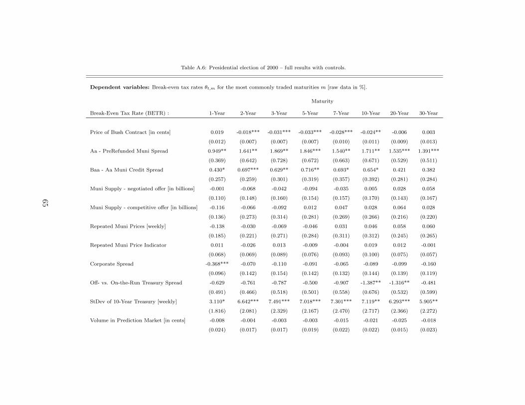
Table A.6: Presidential election of 2000 – full results with controls.


Maturity


Price of Bush Contract [in cents] 0.019 -0.018*** -0.031*** -0.033*** -0.028*** -0.024** -0.006 0.003

(0.012) (0.007) (0.007) (0.007) (0.010) (0.011) (0.009) (0.013)

Aa - PreRefunded Muni Spread 0.949** 1.641** 1.869** 1.846*** 1.540** 1.711** 1.535*** 1.391***

(0.369) (0.642) (0.728) (0.672) (0.663) (0.671) (0.529) (0.511)

Baa - Aa Muni Credit Spread 0.430* 0.697*** 0.629** 0.716** 0.693* 0.654* 0.421 0.382

(0.257) (0.259) (0.301) (0.319) (0.357) (0.392) (0.281) (0.284)

Muni Supply - negotiated offer [in billions] -0.001 -0.068 -0.042 -0.094 -0.035 0.005 0.028 0.058

(0.110) (0.148) (0.160) (0.154) (0.157) (0.170) (0.143) (0.167)

Muni Supply - competitive offer [in billions] -0.116 -0.066 -0.092 0.012 0.047 0.028 0.064 0.028

(0.136) (0.273) (0.314) (0.281) (0.269) (0.266) (0.216) (0.220)

Repeated Muni Prices [weekly] -0.138 -0.030 -0.069 -0.046 0.031 0.046 0.058 0.060

(0.185) (0.221) (0.271) (0.284) (0.311) (0.312) (0.245) (0.265)

Repeated Muni Price Indicator 0.011 -0.026 0.013 -0.009 -0.004 0.019 0.012 -0.001

(0.068) (0.069) (0.089) (0.076) (0.093) (0.100) (0.075) (0.057)

Corporate Spread -0.368*** -0.070 -0.110 -0.091 -0.065 -0.089 -0.099 -0.160

(0.096) (0.142) (0.154) (0.142) (0.132) (0.144) (0.139) (0.119)

Off- vs. On-the-Run Treasury Spread -0.629 -0.761 -0.787 -0.500 -0.907 -1.387** -1.316** -0.481

(0.491) (0.466) (0.518) (0.501) (0.558) (0.676) (0.532) (0.599)

StDev of 10-Year Treasury [weekly] 3.110* 6.642*** 7.491*** 7.018*** 7.301*** 7.119** 6.293*** 5.905**

(1.816) (2.081) (2.329) (2.167) (2.470) (2.717) (2.366) (2.272)

Volume in Prediction Market [in cents] -0.008 -0.004 -0.003 -0.003 -0.015 -0.021 -0.025 -0.018

(0.024) (0.017) (0.017) (0.019) (0.022) (0.022) (0.015) (0.023)

65



Maturity


Units Traded in Prediction Market -0.179 -0.132 -0.153 -0.121 -0.113 -0.103 -0.042 -0.083

(0.117) (0.108) (0.122) (0.109) (0.105) (0.105) (0.082) (0.085)

Observations 131 131 131 131 131 131 131 131

Notes:• Regression results using daily election probabilities for the presidential election of 2000. The tax reform enacted in 2001 reduced

the statutory top income rate by 4.6% from 39.6% to 35% over 5 years and the reform in 2003 accelerated the phase-in period tothree years.

• The contract yields 100 cents if the candidate wins and zero otherwise. Therefore, an increase of the price by 1 cent correspondsto a 1% increase in the perceived probability of the candidate winning the presidential election.

• Newey-West HAC robust standard errors in parentheses. The regression also includes a time trend, month and trading-day fixedeffects, and Treasury interest rates.




66

Table A.7: Presidential election of 1992 – full results with controls.


Maturity


Price of Clinton Contract [in cents] 0.121** 0.075* 0.122*** 0.076*** 0.084*** 0.090*** 0.035** 0.040**

(0.051) (0.044) (0.039) (0.025) (0.021) (0.021) (0.015) (0.017)

Aa - PreRefunded Muni Spread 0.264 0.112 0.142 0.038 0.015 -0.072 -0.026 -0.026

(0.285) (0.126) (0.117) (0.096) (0.080) (0.094) (0.066) (0.067)

A - Aa Muni Credit Spread 0.198 -0.287 -0.309 -0.205 -0.265 -0.260 -0.340** -0.287*

(0.500) (0.303) (0.313) (0.262) (0.264) (0.209) (0.131) (0.160)

Muni Supply - negotiated offer [in billions] 0.023 -0.389** -0.408** -0.268** -0.261** -0.220** -0.068 -0.070

(0.287) (0.174) (0.172) (0.127) (0.104) (0.092) (0.084) (0.089)

Muni Supply - competitive offer [in billions] -1.517* 0.061 0.155 0.252 0.153 0.073 0.177 0.093

(0.861) (0.574) (0.525) (0.438) (0.422) (0.398) (0.180) (0.158)

Repeated Muni Prices [weekly] -0.683 -1.017 -0.465 -0.635 -0.717 -0.921 0.079 0.256

(0.902) (0.638) (0.583) (0.673) (0.618) (0.575) (0.278) (0.449)

Repeated Muni Price Indicator 0.603 0.731*** 0.634*** 0.458*** 0.434*** 0.366** 0.226* 0.210*

(0.438) (0.232) (0.180) (0.149) (0.148) (0.143) (0.122) (0.113)

Corporate Spread -1.271 -1.459** -1.374** -1.134** -1.155** -0.762** -0.433 -0.617**

(1.240) (0.727) (0.649) (0.565) (0.453) (0.378) (0.291) (0.239)

Off- vs. On-the-Run Treasury Spread -1.898 0.545 -0.700 0.214 -0.133 -0.632 0.248 0.356

(1.447) (0.964) (1.050) (0.806) (0.724) (0.759) (0.492) (0.611)

StDev of 10-Year Treasury [weekly] -7.071 -0.283 3.521 7.052** 8.433*** 6.481** -0.754 -0.785

(7.207) (3.462) (3.289) (2.910) (2.858) (2.806) (1.873) (2.429)

Volume in Prediction Market [in cents] 0.174 0.317 0.063 -0.007 -0.047 -0.087 -0.008 0.090

(0.450) (0.317) (0.310) (0.214) (0.245) (0.221) (0.153) (0.163)

67



Maturity


Units Traded in Prediction Market -1.741 -2.391 -0.250 0.270 0.465 0.765 0.090 -0.724

(3.882) (2.652) (2.584) (1.787) (1.999) (1.807) (1.247) (1.328)

Observations 82 82 82 82 82 82 82 82

Notes:• Regression results using daily election probabilities for the presidential election of 1992. The tax reform enacted in 1993 increased

the statutory top income rate by 8.6% from 31% to 39.6% retroactively to January 1, 1993.

• The contract yields 100 cents if the candidate wins and zero otherwise. Therefore, an increase of the price by 1 cent correspondsto an approximately one-percent increase in the perceived probability of the candidate winning the presidential election.

• Newey-West HAC robust standard errors in parentheses. The regression also includes a time trend, month and trading-day fixedeffects, and Treasury interest rates.




68

Table A.8: Consumption response of high-income households in different sub-periods.

Period: 1980-1988 1989-1994 1995-2001

(1) (2) (3)

tax news shock -1.139* -0.138 -1.587***

(0.656) (0.918) (0.542)

age -0.005 -0.029 -0.001

(0.052) (0.060) (0.059)

age2/1000 -0.060 0.177 0.060

(0.591) (0.674) (0.667)

∆ adults 1.785*** 2.650*** 1.615***

(0.389) (0.418) (0.436)

∆ kids 1.030** -0.436 1.481***

(0.467) (0.454) (0.457)

monthly FEs Yes Yes Yes

R2 0.022 0.025 0.015

Notes: Reported standard errors in parentheses areadjusted for within-household correlations and het-eroskedasticity.




69

Table A.9: Consumption response of high-income households: different filtering.

Time series filter: no filter one-sided two-sided

(1) (2) (3)

tax news shock 0.013 -0.859** -1.147***

(0.116) (0.341) (0.377)

age -0.014 -0.011 -0.012

(0.032) (0.032) (0.032)

age2/1000 0.073 0.044 0.056

(0.365) (0.365) (0.365)

∆ adults 1.961*** 1.959*** 1.960***

(0.239) (0.239) (0.239)

∆ kids 0.767*** 0.771*** 0.772***

(0.268) (0.268) (0.268)


R2 0.020 0.020 0.020

Notes: Column (1) applies no times series filter tothe bond data, (2) applies a one-sided filter, while(3) applies a two-sided filter. Reported standard er-rors in parentheses are adjusted for within-householdcorrelations and heteroskedasticity.




70

Table A.10: Consumption response as a function of the size of the tax news shock.

Size of news shock: 50% largest 25% most 25% most(in abs. value) negative positive

(1) (2) (3)

tax news shock -1.125*** -0.910** -0.880*

(0.359) (0.418) (0.511)

age 0.001 0.034 -0.009

(0.043) (0.053) (0.052)

age2/1000 -0.051 -0.524 0.138

(0.494) (0.609) (0.592)

∆ adults 2.156*** 1.835*** 2.497***

(0.324) (0.407) (0.398)

∆ kids 1.095*** 1.185*** 0.797*

(0.351) (0.422) (0.462)


R2 0.020 0.018 0.020

Notes: Reported standard errors in parentheses are ad-justed for within-household correlations and heteroskedas-ticity.




71

Table A.11: Consumption response as a function of liquid wealth.

LW>2% of TAE LW∈ (0, 0.2%) of TAE LW=0

(1) (2) (3)

tax news shock -0.510* 0.457 -0.486

(0.301) (0.861) (0.346)

age -0.008 -0.087 -0.054

(0.035) (0.097) (0.044)

age2/1000 -0.021 1.029 0.582

(0.384) (1.136) (0.499)

∆ adults 2.090*** 2.490*** 2.069***

(0.304) (0.659) (0.316)

∆ kids 0.991*** -0.089 1.083***

(0.373) (0.568) (0.341)


R2 0.021 0.059 0.021

Notes: TAE are total annual expenditures. LW is liquid wealth and isdefined as the sum of checking and savings accounts. Reported standarderrors in parentheses are adjusted for within-household correlations andheteroskedasticity.




72

Table A.12: Consumption response as a function of education.

High School College

tax news shock 0.222 -0.870***(0.309) (0.287)

age -0.008 -0.031

(0.034) (0.032)

age2/1000 -0.015 0.342

(0.384) (0.368)

∆ adults 2.268*** 2.216***

(0.249) (0.270)

∆ kids 1.333*** 0.861***

(0.277) (0.297)

monthly FEs Yes Yes

R2 0.021 0.020

Notes: High School includes households witha high school degree or less, while College in-cludes households with at least a college de-gree. Reported standard errors in parenthesesare adjusted for within-household correlationsand heteroskedasticity.




73

Appendix B

Figures

74

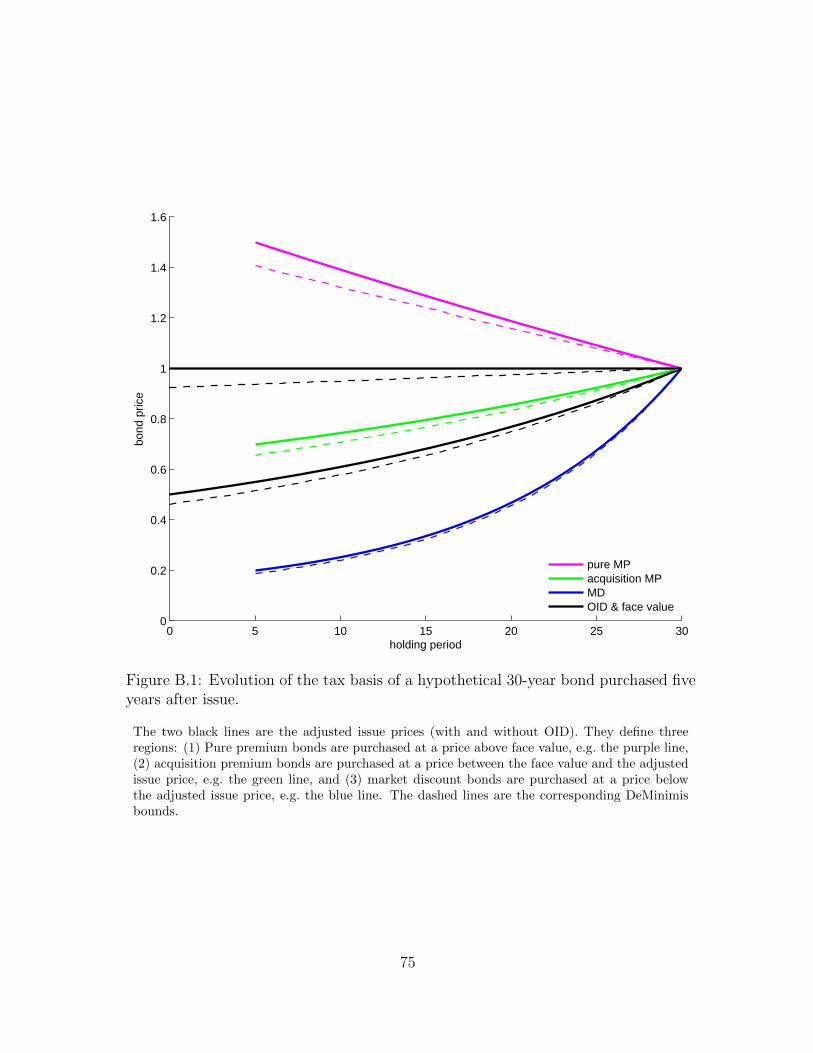
0 5 10 15 20 25 300

0.2

0.4

0.6

0.8

1

1.2

1.4

1.6

holding period

bond

pric

e

pure MPacquisition MPMDOID & face value

Figure B.1: Evolution of the tax basis of a hypothetical 30-year bond purchased fiveyears after issue.

The two black lines are the adjusted issue prices (with and without OID). They define threeregions: (1) Pure premium bonds are purchased at a price above face value, e.g. the purple line,(2) acquisition premium bonds are purchased at a price between the face value and the adjustedissue price, e.g. the green line, and (3) market discount bonds are purchased at a price belowthe adjusted issue price, e.g. the blue line. The dashed lines are the corresponding DeMinimisbounds.

75

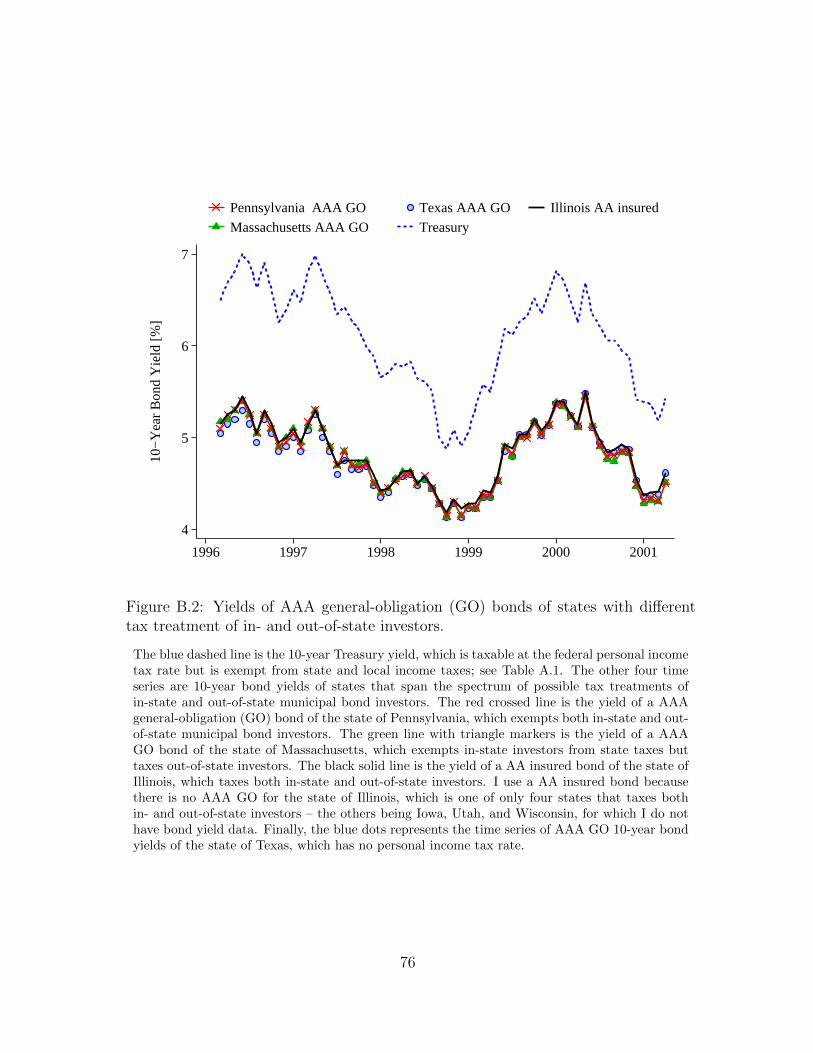
4

5

6

7

10−

Yea

r B

ond

Yie

ld [%

]

1996 1997 1998 1999 2000 2001

Pennsylvania AAA GO Texas AAA GO Illinois AA insured

Massachusetts AAA GO Treasury

Figure B.2: Yields of AAA general-obligation (GO) bonds of states with differenttax treatment of in- and out-of-state investors.

The blue dashed line is the 10-year Treasury yield, which is taxable at the federal personal incometax rate but is exempt from state and local income taxes; see Table A.1. The other four timeseries are 10-year bond yields of states that span the spectrum of possible tax treatments ofin-state and out-of-state municipal bond investors. The red crossed line is the yield of a AAAgeneral-obligation (GO) bond of the state of Pennsylvania, which exempts both in-state and out-of-state municipal bond investors. The green line with triangle markers is the yield of a AAAGO bond of the state of Massachusetts, which exempts in-state investors from state taxes buttaxes out-of-state investors. The black solid line is the yield of a AA insured bond of the state ofIllinois, which taxes both in-state and out-of-state investors. I use a AA insured bond becausethere is no AAA GO for the state of Illinois, which is one of only four states that taxes bothin- and out-of-state investors – the others being Iowa, Utah, and Wisconsin, for which I do nothave bond yield data. Finally, the blue dots represents the time series of AAA GO 10-year bondyields of the state of Texas, which has no personal income tax rate.

76

10

20

30

40

50

60

1980 1985 1990 1995 20001977 2004

2yr BETR (trend) 15yr BETR (trend)

top 1% tax rate 33% tax bubble (’88−’90)

Figure B.3: 2-year and 15-year break-even tax rates (BETR) θt,2 and θt,15 againstthe marginal tax rate of the top 1%.

The thin lines are the raw data and the thick lines are the corresponding low frequency compo-nents of the 2-year and the 15-year break-even tax rates, respectively, corresponding to equation(2.3). The blue thin dashed line is the top 1% tax rate taken from Saez (2004). The solid blueline is the ‘33% tax bubble’ during the years 1988-1990; in this period, the top marginal tax rateis higher than the marginal tax rate of the top 1% of the income distribution.

77

20

30

40

50

60

70

mar

gina

l tax

rat

e

1980 1982 1985 1988 1991 1994 1997 2000 2003 2006

marginal investor (SCF) +2 SEs/−2 SEs

top 1% of income (Saez) top 5−1% of income (Saez)

top 5% of income (Saez) highest statutory rate

Figure B.4: Average Marginal Tax Rate of the Marginal Investors calculated fromthe Survey of Consumer Finances (SCF).

The blue dots are the estimated marginal tax rate of the marginal investor defined as the asset-weighted average of the effective marginal tax rates over all households that own both taxableand tax-exempt bonds. Two standard error bands are shown around the point estimates of themarginal investor’s marginal tax rate. The black lines are the marginal tax rates of differentpercentiles of the income distribution taken from Saez (2004).

78

2000 2005 2010 2015 2020 2025 2030−5

−4

−3

−2

−1

0

1

2

3

currentyear ↓

counterfactual ifE[τ |Gore] = τ2000

↓

assuming Bush tax cuts expire

↑

assuming Bush tax cuts become permanent↓

Newey-West 95% confidence band↓

← point estimates β

perfect foresight coefficients βpf

↓

forecasting horizon m during presidential election of 2000

changein

break-even

taxrate

[%]

Figure B.5: Path of Break-Even Tax Rates during presidential election of 2000.

The black line is the estimated response of the break-even tax rates β from regression equation(2.6) to changes in the election probability of George W. Bush during the five months prior toElection Day in 2000; the black dashed lines are 95% Newey-West confidence bands. The bluelines show the population coefficients βpf one should obtain under perfect foresight and assumingthat the counter-factual path of tax rates under President Gore is fixed at τ2000 = 39.6%. Twoscenarios for the path of future tax rates beyond 2011 are shown, one where the Bush tax cutsexpire in 2011 as scheduled and one where they become permanent.

79

1992 1995 2000 2005 2010 2015 2020 2022

0

2

4

6

88.6

10

12

14

16 EGTRRA → ← JGTRRA

← Newey-West 95% confidence band

currentyear ↓

counterfactual ifE[τ |H.Bush] = τ1992

↓

assuming W.Bush tax cuts expire

↓

assuming W.Bush tax cuts become permanent↑

perfect foresight coefficients βpf

↓

տpoint estimates β


changein

break-even

taxrate

[%]

Figure B.6: Path of Break-Even Tax Rates during presidential election of 1992.

The black line is the estimated response of the break-even tax rates β from regression equation(2.6) to changes in the election probability of Bill Clinton during the three months prior toElection Day in 1992; the black dashed lines are 95% Newey-West confidence bands. The bluelines show the population coefficients βpf one should obtain under perfect foresight and assumingthat the counter-factual path of tax rates under President H. Bush is fixed at τ1992 = 31%. Twoscenarios for the path of future tax rates beyond 2011 are shown, one where the W. Bush tax cutsexpire in 2011 as scheduled and one where they become permanent. The two vertical lines showthe enactment dates of the tax reforms in 2001 and 2003, EGTRRA and JGTRRA respectively.

80

2000 2005 2010 2015 2020 2025 2030

35

36

37

38

39

39.6

40

41

currentyear↓

counterfactual ifE[τ |Gore] = τ2000

↓

path of perfect foresight tax rates τ↓

assuming Bush tax cuts expire

↑

տ assuming Bush tax cuts become permanent

← path of expected tax rates in 2000: E[τ |∆Bush] + τ1992


taxrate

[%]

Figure B.7: Path of Expected Tax Rates during presidential election of 2000.

The black line is the expected tax path recovered by inverting equation (2.7) with a ridge re-gression with optimal regularization parameter µ = 0.15. The top rate in 2000 is added to theexpected changes in the tax path to make it comparable to the ex-post realization of the taxpath; see Figure B.5 for the definition of the two blue lines.

81

1992 1995 2000 2005 2010 2015 202226

28

30

31

32

34

36

38

39.6

42

44

46

current year↓

counterfactual ifE[τ |H. Bush] = τ1992

↓

← path of perfect foresight tax rates τ

assuming W.Bush tax cuts expire↓

assuming W.Bush tax cuts become permanent↓

←path of expected tax rates in 1992:

E[τ |∆Clinton] + τ1992


taxrate

[%]

Figure B.8: Path of Expected Tax Rates during presidential election of 1992.

The black line is the expected tax path recovered by inverting equation (2.7) with a ridge re-gression with optimal regularization parameter µ = 0.05. The top rate in 1992 is added to theexpected changes in the tax path to make it comparable to the ex-post realization of the taxpath; see Figure B.6 for the definition of the two blue lines.

82

5

10

15

20

Ave

rage

Bre

ak−

Eve

n T

ax P

rem

ium

1 5 10 15 20 25 30maturity

Figure B.9: Average break-even tax premium E[Λt] as a function of the maturity;see equation (2.9).

83

1978 1982 1987 199220

30

40

50

60

current date: 01/1977

forecasting horizon

expe

cted

vs

actu

al ta

x ra

tes

[%]

path of market-based expected tax rate↓

↑path of actual (perfect-foresight) tax rate of top 1%

1979 1983 1988 199320

30

40

50

60


forecasting horizon

expe

cted

vs

actu

al ta

x ra

tes

[%]

1980 1984 1989 199420

30

40

50

60


forecasting horizon

expe

cted

vs

actu

al ta

x ra

tes

[%]

1981 1985 1990 199520

30

40

50

60


forecasting horizon

expe

cted

vs

actu

al ta

x ra

tes

[%]

1982 1986 1991 199620

30

40

50

60


forecasting horizon

expe

cted

vs

actu

al ta

x ra

tes

[%]

1983 1987 1992 199720

30

40

50

60


forecasting horizon

expe

cted

vs

actu

al ta

x ra

tes

[%]

path of actual (perfect-foresight) tax rate of top 1%↓

↑path of market-based expected tax rate

Figure B.10: Anticipation of the Reagan Tax Cuts (ERTA 1981 and TRA 1986)between January 1977 and January 1982.

This figure shows the evolution of the path of expected tax rates between 1977 and 1982 in therun-up to the first Reagan tax cut (ERTA 1981). The dashed line, which represents the perfect-foresight tax path, is the marginal tax rate of the top 1% of the income distribution taken fromSaez (2004). The bond market did not anticipate the Reagan tax cuts until the election year of1980. However, the bond prices already incorporate the second Regan tax cut (TRA 1986) bythe end of 1981. The web appendix of this paper – https://sites.google.com/site/lorenzkueng/ –contains a video of the evolution of Et[τ ] from January 1977 to August 1982 that shows monthlychanges in the path of expected tax rates.

84

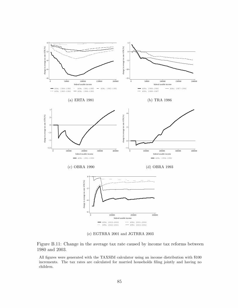
https://sites.google.com/site/lorenzkueng/

−8

−6

−4

−2

0ch

ange

in a

vera

ge ta

x ra

te A

TR

[%]

0 50000 100000 150000 200000

federal taxable income

ATR: 1984−1980 ATR: 1981−1980 ATR: 1982−1981

ATR: 1983−1982 ATR: 1984−1983

(a) ERTA 1981

−15

−10

−5

0

5

chan

ge in

ave

rage

tax

rate

AT

R [%

]

0 50000 100000 150000 200000


ATR: 1988−1986 ATR: 1987−1986

ATR: 1988−1987

(b) TRA 1986

−1.5

−1

−.5

0

.5

1

chan

ge in

ave

rage

tax

rate

AT

R [%

]

0 100000 200000 300000 400000


ATR: 1991−1990

(c) OBRA 1990

−1

0

2

4

chan

ge in

ave

rage

tax

rate

AT

R [%

]

0 100000 200000 300000 400000


ATR: 1994−1992

(d) OBRA 1993

−6

−4

−2

0

chan

ge in

ave

rage

tax

rate

AT

R [%

]

0 100000 200000 300000


ATR: 2003−2000 ATR: 2001−2000

ATR: 2002−2001 ATR: 2003−2002

(e) EGTRRA 2001 and JGTRRA 2003

Figure B.11: Change in the average tax rate caused by income tax reforms between1980 and 2003.

All figures were generated with the TAXSIM calculator using an income distribution with $100increments. The tax rates are calculated for married households filing jointly and having nochildren.

85

−15

−10

−5

0

basi

s po

ints

1993 1994 1995 1996 1997 1998 1999 2000 2001

Figure B.12: Spread between AAA general-obligation and pre-refunded municipalbonds with 7-year maturity.

86

0

100

200

300

400

500

basi

s po

ints

2005 2006 2007 2008 2009 2010

Maryland AAA GO CDS US Treasury CDS

Berkshire Hathaway CDS

Figure B.13: Credit Default Swap (CDS) of 10-year Treasury, municipal, and corpo-rate bonds.

Source: Credit Market Analysis (CMA) taken from Datastream.

87

20

30

40

50

60

1985 1990 1995 20001980

two−sided filter one−sided filter

no filter

Figure B.14: Different filtering of the time series of 2-year break-even tax rates.

88

Figure B.15: Municipal Debt Ownership

Source: Ang et al. (2007), based on the Flow of Funds Accounts provided by the Board of Gov-ernors.Percentage of outstanding municipal bonds held (i) by households, which includes direct owner-ship and indirect ownership through mutual funds, money market funds, and closed-end funds,(ii) by banks, which comprise commercial banks and savings institutions, and (iii) by insurancecompanies, which are life insurance companies and other insurance companies.

89

0.0

5.0

10.0

15.0

20.0

25.0

30.0

35.0

40.0

1979

1981

1983

1985

1987

1989

1991

1993

1995

1997

1999

2001

2003

2005

2007

top 1%top 5%top 10%top 20%

Figure B.16: Total federal Average Tax Rates 1977-2007

Source: Congressional Budget Office (CBO).This figure shows the time series of effective total federal average tax rates between 1977 and2007 for households in different income percentiles. It motivates the definition of the sample ofhigh-income households used in the paper. The average tax rates are highly but not perfectlycorrelated. Hence, news about the evolution of the marginal income tax rate of the marginalmunicipal bond investor is informative for the households’ average tax rates, while at the sametime allowing for time fixed effects in the estimation.

90

Bibliography

Abowd, John M. and David Card, “On the Covariance Structure of Earnings andHours Changes,” Econometrica, 1989, 57 (2), 411–445.

Agarwal, Sumit, Chunlin Liu, and Nichola S. Souleles, “The Reaction of ConsumerSpending and Debt to Tax Rebates: Evidence from Consumer Credit Data,” Jour-nal of Political Economy, 2007, 115 (6), 986–1019.

Akerlof, George A. and Janet L. Yellen, “A Near-Rational Model of the BusinessCycle, with Wage and Price Inertia,” Quarterly Journal of Economics, 1985, 100(Supplement), 823–838.

Ang, Andrew and Francis A. Longstaff, “Systemic Sovereign Credit Risk: Lessonsfrom the U.S. and Europe,” Working Paper, 2011.

, Vineer Bhansali, and Yuhang Xing, “Taxes on Tax-Exempt Bonds,” WorkingPaper, 2007.

Aster, Richard C., Brian Brochers, and Clifford H. Thurber, Parameter Estimationand Inverse Problems, Elsevier Academic Press, 2005.

Attanasio, Orazio, “Consumption,” Handbook of Macroeconomics, 1999, 1, 741–812.

Auerbach, Alan J and Joel Slemrod, “The Economic Effects of the Tax Reform Actof 1986,” Journal of Economic Literature, 1997, 35 (2), 589–632.

Ayers, Benjamin C., Bryan C. Cloyd, and John B. Robinson, ““Read My Lips ...”:Does the Tax Rethoric of Presidential Candidates Affect Security Prices?,” Journalof Law and Economics, 2005, 48 (1), 125–148.

Barsky, Robert B. and Eric R. Sims, “Information, Animal Spirits, and the Meaningof Innovations in Consumer Confidence,” American Economic Review, forthcom-ing.

Batchelor, Roy and Pami Dua, “Survey Expectations in the Time Series Consump-tion Function,” Review of Economics and Statistics, 1992, 74 (4), 598–606.

91

BIBLIOGRAPHY

Beaudry, Paul and Franck Portier, “News, Stock Prices and Economic Fluctuations,”American Economic Review, 2006, 96 (4), 1293–1307.

Blanchard, Olivier J, Jean-Peaul L’Huillier, and Guido Lorenzoni, “News, Noise, andFluctuations: An Empirical Exploration,” NBER Working Paper No. 15015, 2009.

Blinder, Alan S. and Angus Deaton, “The Time Series Consumption Function Re-visited,” Brookings Papers on Economic Activity, 1985, 1985 (2), 465–521.

Branch, Raphael E., “The Consumer Expenditure Survey: a comparative analysis,”Monthly Labor Review, 1994, 117, 47–55.

Calmes, Jackie, “Bush Promotes Big Tax Cuts in a Move To Attract Middle-ClassSwing Voters,” The Wall Street Journal, 2000, Monday, Septermber 25, A.16.

Campbell, John Y. and Angus Deaton, “Why is Consumption So Smooth?,” Reviewof Economic Studies, 1989, 56 (3), 357.

and Gregory N. Mankiw, “Consumption, Income, and Interest Rates: Reinter-preting the Time Series Evidence,” NBER Macroeconomics Annual, 1989.

Chalmers, John M.R., “Default Risk Cannot Explain the Muni–Puzzle: Evidencefrom Bonds that Are Secured by U.S. Treasury Obligation,” Review of FinancialStudies, 1998, 11 (2), 281–308.

, “Systematic Risk and the Muni Puzzle,” National Tax Journal, 2006.

Chetty, Raj, “Is the Taxable Income Elasticity Sufficient to Calculate DeadweightLoss? The Implications of Evasion and Avoidance,” American Economic Journal: Economic Policy, 2009, 1 (2), 31–52.

Cochrane, John H., “The Sensitivity of Tests of the Intertemporal Allocation ofConsumption to Near-Rational Alternatives,” American Economic Review, 1989,79 (3), 319–337.

, “Shocks,” Carnegie-Rochester Conference Series on Public Policy, December1994, 41, 295–364.

Coibion, Olivier and Yuriy Gorodnichenko, “Information Rigidity and the Expecta-tions Formation Process: A Simple Framework and New Facts,” NBER WorkingPaper No. 16537, 2011.

Constantinides, Geroge M. and Jonathan E. Ingersoll, “Optimal Bond Trading withPersonal Taxes,” Journal of Finance, 1984, 13 (3), 299–335.

Deaton, Angus, Understanding Consumption, Oxford University Press, 1992.

92

BIBLIOGRAPHY

English, William B., “Understanding the Costs of Sovereign Default: American StateDebts in the 1840’s,” American Economic Review, 1996, 86, 259 – 275.

Fabozzi, Frank J., Fixed Income Securities, 2 ed., John Wiley & Sons, 2002.

and David Z. Nirenberg, “Federal Income Tax Treatment of Fixed Income Secu-rities,” in Frank J. Fabozzi, Dessa T. Fabozzi, and Irving M. Pollack, eds., TheHandbook of Fixed Income Securities, 1991.

Fama, Eugene F., “A Pricing Model of the Municipal Bond Market,” Working Paper,1977.

Feenberg, Daniel R. and Elizabeth Coutts, “An Introduction to the TAXSIM Model,”Journal of Policy Analysis and Management, 1993, 12 (1), 189–194.

and James M. Poterba, “Which Households Own Municipal Bonds? EvidenceFrom Tax Returns,” National Tax Journal, 1991, 44 (4), 93–103.

Feldstein, Martin, “The Effect of Marginal Tax Rates on Taxable Income: A PanelStudy of the 1986 Tax Reform Act,” Journal of Political Economy, 1995, 103 (3),551–572.

, “Tax Avoidance and the Deadweight Loss of the Income Tax,” Review of Eco-nomics and Statistics, 1999, 81 (4), 674–680.

Fortune, Peter, “Do Municipal Bond Yields Forecast Tax Policy?,” New EnglandEconomic Review, 1996.

Fuhrer, Jeffrey C., “On the Information Content of Consumer Survey Expectations,”Review of Economics and Statistics, 1988, 70 (1), 140–144.

Giglio, Stefano, “Credit Default Swap Spreads and Systemic Financial Risk,” Work-ing Paper, 2011.

Gorodnichenko, Yuriy, Jorge Martinez-Vazquez, and Klara Sabirianova Peter, “Mythand Reality of Flat Tax Reform: Micro Estimates of Tax Evasion Response andWelfare Effects in Russia,” Journal of Political Economy, 2009, 117 (3), 504–554.

Green, Richard C., “A Simple Model of the Taxable and Tax-Exempt Yield Curves,”Review of Financial Studies, 1993, 6 (2), 233–264.

Gurkaynak, Refet S., Brian Sack, and Jonathan H. Wright, “The U.S. Treasuryyield curve: 1961 to the present,” Journal of Monetary Economics, 2007, 54 (8),2291–2304.

93

BIBLIOGRAPHY

Hansen, Lars Peter, William T. Roberds, and Thomas J. Sargent, “Time SeriesImplications of Present Value Budget Balance and of Martingale Models of Con-sumption and Taxes,” in Lars Peter Hansen and Thomas J. Sargent, eds., RationalExpectations Econometrics, Boulder and Oxford: Westview Pres, 1991, pp. 121–61.

Harris, Lawrence E. and Michael S. Piwowar, “Municipal Bond Liquidity,” WorkingPaper, 2004.

Hausman, Jerry A. and James M. Poterba, “Household Behavior and the Tax ReformAct of 1986,” Journal of Economic Perspectives, 1987, 1 (1), 101–119.

Hayashi, Fumio, Understanding Saving: Evidence from the United States and Japan,The MIT Press, 1997.

Hempel, George H., The Postwar Quality of State and Local Debt, Columbia Univer-sity Press, 1971.

Jaimovich, Nir and Sergio Rebelo, “Can News about the Future Drive the BusinessCycle?,” American Economic Review, 2009, 99 (4), 1097–1118.

Jappelli, Tullio and Luigi Pistaferri, “The Consumption Response to IncomeChanges,” Annual Review of Economics, 2010, 2, 479–506.

Johnson, David S., Jonathan A. Parker, and Nicholas S. Souleles, “Household Expen-diture and the Income Tax Rebates of 2001,” American Economic Review, 2006,96 (5), 1589–1610.

Kochin, Levis A. and Richard W. Parks, “Was the Tax-Exempt Bond Market Inef-ficient or Were Future Expected Tax Rates Negative?,” Journal of Finance, 1988,43, 913 – 931.

Kramer, Andrea S., Financial Products: Taxation, Regulation and Design, AspenPublishers, 2003.

Kueng, Lorenz, “News from Alaska: Do Households Respond to Return News ratherthan Dividend Payments?,” Working Paper, 2012.

Leeper, Eric M., Todd B. Walker, and Shu-Chun S. Yang, “Foresight and InformationFlows,” NBER Working Paper No. 16951, 2011.

Longstaff, Francis A., “Municipal Debt and Marginal Tax Rates: Is There a TaxPremium in Asset Prices?,” Journal of Finance, 2011, 66, 721–751.

Lorenzoni, Guido, “News and Aggregate Demand Shocks,” Annual Review of Eco-nomics, 2011, 3, 537–557.

94

BIBLIOGRAPHY

Lusardi, Annamaria, “Permanent Income, Current Income, and Consumption: Ev-idence from Two Panel Data Sets,” Journal of Business & Economic Statistics,1996, 14 (1), 81–90.

MaCurdy, Thomas E., “The Use of Time Series Processes to Model the Error Struc-ture of Earnings in a Longitudinal Data Analysis,” Journal of Econometrics, 1982,18 (1), 83–114.

Mankiw, N. Gregory and James M. Poterba, “Stock Market Yields and the Pricingof Municipal Bonds,” NBER Working Paper No. 5607, 1996.

and Ricardo Reis, “Sticky Information Versus Sticky Prices: A Proposal to Re-place the New Keynesian Phillips Curve,” Quarterly Journal of Economics, 2002,117 (4), 1295–1328.

Meghir, Costas and Luigi Pistaferri, “Income Variance Dynamics and Heterogeneity,”Econometrica, 2004, 72 (1), 1–32.

Mehra, Yash P., “The Output Gap, Expected Future Inflation and Inflation Dynam-ics: Another Look,” The BE Journal of Macroeconomics, 2004, 4 (1), 1–17.

Park, Sangkyun, “The Relationship between Government Financial Condition andExpected Tax Rates Reflected in Municipal Bond Yields,” Federal Reserve Bankof New York Staff Reports, 1995.

Parker, Jonathan A., “The Reaction of Household Consumption to PredictableChanges in Social Security Taxes,” American Economic Review, 1999, 89 (4).

Pistaferri, Luigi, “Superior Information, Income Shocks, and the Permanent IncomeHypothesis,” Review of Economics and Statistics, 2001, 83 (3), 465–476.

Poterba, James M., Explaining the Yield Spread between Taxable and Tax-exemptBonds: The Role of Expected Tax Policy, The University of Chicago Press, 1986.

, “Are Consumers Forward Looking? Evidence from Fiscal Experiments,” Ameri-can Economic Review Papers and Proceedings, 1988, 78 (2), 413–418.

Ravn, Morten O. and Harald Uhlig, “On Adjusting the Hodrick-Prescott Filter forthe Frequency of Observations,” Review of Economics and Statistics, 2002, 84 (2),371–376.

Reinhart, Carmen and Kenneth Rogoff, “The Forgotten History of Domestic Debt,”Economic Journal, 2011, 121, 319 – 350.

Reis, Ricardo, “Inattentive consumers,” Journal of Monetary Economics, 2006, 53(8), 1761–1800.

95

BIBLIOGRAPHY

Romer, Christina D. and David H. Romer, “A Narrative Analysis of Postwar TaxChanges,” online appendix to Romer and Romer (American Economic Review2010), ”The Macroeconomic Effects of Tax Changes: Estimates Based on a NewMeasure of Fiscal Shocks”, 2008.

and , “The Macroeconomic Effects of Tax Changes: Estimates Based on a NewMeasure of Fiscal Shocks,” American Economic Review, 2010, 100 (3), 763–801.

Runkle, David E., “Liquidity Constraints and the Permanent-Income Hypothesis:Evidence from Panel Data,” Journal of Monetary Economics, 1997, 27, 73 – 98.

Saez, Emmanuel, “Reported Incomes and Marginal Tax Rates, 1960-2000: Evidenceand Policy Implications,” NBER Working Paper No. 10273, 2004.

Schmitt-Grohe, Stephanie and Martin Uribe, “What’s News in Business Cycles,”Working Paper, 2010.

Seib, Gerald F. and Alan Murray, “Where They Stand: A Voters’ Guide to theCandidates and the Issues,” The Wall Street Journal, 1992, Monday, Septermber21, R6.

Shapiro, Matthew D. and Joel Slemrod, “Consumer Response to the Timing of In-come: Evidence from a Change in Tax Withholding,” American Economic Review,1995, 85 (1), 274–283.

and , “Did the 2001 Tax Rebate Stimulate Spending? Evidence from TaxpayerSurveys,” Tax Policy and the Economy, 2003, 17, 83–109.

Sims, Christopher A., “Implications of rational inattention,” Journal of MonetaryEconomics, 2003, 50 (3), 665–690.

Slemrod, Joel and Timothy Greimel, “Did Steve Forbes scare the US municipal bondmarket?,” Journal of Public Economics, 1999, 74 (1), 81–96.

Snowberg, Erik, Justin Wolfers, and Eric Zitzewitz, “How Prediction Markets CanSave Event Studies,” NBER Working Paper No. 16949, 2011.

Souleles, Nicholas S., “The Response of Household Consumption to Income TaxRefunds,” American Economic Review, 1999, 89 (4), 947–958.

, “Consumer response to the Reagan tax cuts,” Journal of Public Economics, 2002,85 (1), 99–120.

Temel, Judy W., The Fundamentals of Municipal Bonds, 5 ed., John Wiley & Sons,2001.

96

BIBLIOGRAPHY

Wolff, Edward N., “Recent Trends in Household Wealth in the United States: RisingDebt and the Middle-Class Squeeze – an Update to 2007,” Working Paper, 2010.

Woodford, Michael, “Imperfect Common Knowledge and the Effects of MonetaryPolicy,” in Philippe Aghion, Roman Frydman, Joseph Stiglitz, and Michael Wood-ford, eds., Knowledge, Information and Expectations in Modern Macroeconomics,Princeton University Press, 2002.

Zeldes, Stephen P., “Consumption and Liquidity Constraints: An Empirical Investi-gation,” Journal of Political Economy, 1989, 97 (2), 305–346.

97

Expected Taxes and Household Consumption Behavior by ...

Documents

Transcript of Expected Taxes and Household Consumption Behavior by ...